Estimation of Q-matrix for DINA Model Using the Constrained

Generalized DINA Framework

Huacheng Li

Submitted in partial fulfillment of the

requirements for the degree of

Doctor of Philosophy

under the Executive Committee

of the Graduate School of Arts and Sciences

COLUMBIA UNIVERSITY

2016

©2016

Huacheng Li

All rights reserved

ABSTRACT

Estimation of Q-matrix for DINA Model Using the Constrained

Generalized DINA Framework

Huacheng Li

The research of cognitive diagnostic models (CDMs) is becoming an important field of

psychometrics. Instead of assigning one score, CDMs provide attribute profiles to indicate the

mastering status of concepts or skills for the examinees. This would make the test result more

informative. The implementation of many CDMs relies on the existing item-to-attribute

relationship, which means that we need to know the concepts or skills each item requires. The

relationships between the items and attributes could be summarized into the Q-matrix.

Misspecification of the Q-matrix will lead to incorrect attribute profile. The Q-matrix can be

designed by expert judgement, but it is possible that such practice can be subjective. There

are previous researches about the Q-matrix estimation. This study proposes an estimation

method for one of the most parsimonious CDMs, the DINA model. The method estimates the

Q-matrix for DINA model by setting constraints on the generalized DINA model. In the

simulation study, the results showed that the estimated Q-matrix fit better the empirical

fraction subtraction data than the expert-design Q-matrix. We also show that the proposed

method may still be applicable when the constraints were relaxed.

i

Table of Contents

List of Tables iii

List of Figures iv

Chapter 1 Introduction 1

1.1 Background ....................................................................................................... 1

1.2 Cognitive Diagnostic Models ........................................................................... 3

Chapter 2 Literature Review 8

2.1 CDMs ................................................................................................................ 8

2.1.1 The DINA model ........................................................................................ 9

2.1.2 The DINO model ...................................................................................... 11

2.1.3 G-DINA model ......................................................................................... 12

2.2 Q-Matrix Diagnostics and Estimation ............................................................ 14

2.2.1 Estimation of Q-matrix ............................................................................. 14

2.2.2 Diagnostics of Q-Matrix ........................................................................... 18

2.3 Bayesian statistics ........................................................................................... 19

2.4 Markov chain Monte Carlo methods .............................................................. 22

ii

Chapter 3 Methods 28

3.1 Model specification and Notation ................................................................... 28

3.2 Estimating the Q-matrix .................................................................................. 31

3.3 Re-labeling and Finalizing Q-matrix .............................................................. 35

3.4 Study designs .................................................................................................. 37

Chapter 4 Results 42

4.1 Simulation Study Results ................................................................................ 42

4.1.1 Results for one simulated data set ............................................................ 43

4.1.2 Results of all simulations ......................................................................... 48

4.2 Empirical Study .............................................................................................. 52

Chapter 5 Discussion 59

5.1 Implication of the study .................................................................................. 59

5.2 Limitation ........................................................................................................ 61

5.3 Possible topics for future research .................................................................. 63

Bibliography 66

Appendix 70

iii

List of Tables

3.1 Q-matrix for Simulation Studies ........................................................................... 39

3.2 Designed Q-matrix for Empirical Studies............................................................. 41

4.1 Estimated Q-matrix for the simulated data ........................................................... 44

4.2 Correlation matrix of Attributes and Column average .......................................... 45

4.3 Simulation design and output summary ................................................................ 49

4.4 Logistic regression outputs ................................................................................... 49

4.5 Simultaneous Test ................................................................................................. 50

4.6 Simulation output summary with improved cutoff ............................................... 52

4.7 Simultaneous Test with improved cutoff .............................................................. 52

4.8 Permutation for estimated Q-matrix ..................................................................... 55

4.9 Minimum difference of the four estimations on empirical data ........................... 56

4.10 Designed Q-matrix and the estimated Q-matrix .................................................. 56

4.11 Result comparison with Chung’s study ................................................................ 57

4.12 Result comparison with Chung’s study................................................................ 58

iv

List of Figures

4.1 Moving average of the estimated Q-matrix ........................................................... 44

4.2 Sampled values of item parameters for item 1....................................................... 46

4.3 Moving averages of item parameters for item 1 .................................................... 47

4.4 Log-likelihood of sampled classes for item 22 ...................................................... 48

4.5 Average bias of the guessing parameter ................................................................. 51

4.6 Average Bias of the attribute effect parameter ....................................................... 51

4.7 Correctness of estimated Q-matrix in Estimation one ........................................... 55

v

Acknowledgements

It is a genuine pleasure to express my deepest sense of thanks to my advisor Prof. Matthew S.

Johnson. This dissertation could not have been prepared or finished without his constant

guidance and support. I am truly indebted and thankful to his advice and encouragement

during my graduate study.

I wish to express my appreciative thanks to the members of the supervisory committee,

Prof. Hsu-Min Chiang, Prof. Young-Sun Lee, Prof. Jingchen Liu, and Prof. Bryan Keller. I

am very grateful to their time, comments and constructive suggestions on the revisions of my

dissertation.

I would like to extend my thanks to all the faculty and staff in Human Development

Department at Teachers College of Columbia University. I am very thankful for the collegial

support over these years from Dr. Meng-ta Chung, Mr. Zhuangzhuang Han, Mr. Xiang Liu,

Dr. Jung Yeon Park, Dr. Rui Xiang and Dr. Jianzhou Zhang.

Finally, I am extremely thankful to my parents and my wife for the never once wavering in

the complete support and for being with me through every step of this incredible journey.

vi

To my family

1

Chapter 1

Introduction

1.1 Background

Psychometrics is a field of study concerned with the theory and the technique of

psychological measurement. It can be used to evaluate respondent attributes such as

knowledge, abilities, attitudes or educational achievement, and to investigate the

characteristics of assessment items. Two kinds of widely used models for such purposes are

Classical Testing Theory (CTT) and the Item Response Theory (IRT). CTT assumes each

respondent has a true score for the attribute, and the observed total score is decomposed into

the true score and a measurement error. Based on this assumption, one can calculate the test

reliability, item difficulty (i.e., proportion correct) and item discrimination (i.e., point biserial

correlations). The classical item statistics such as the item difficulty, the item discrimination

and the test statistics such as test reliability are dependent on the examinee sample in which

they are obtained (Hambleton & Jones, 1993). This is considered as a shortcoming of CTT in

that examinee characteristics and test characteristics cannot be separated. Another

shortcoming is that CTT is test oriented rather than item oriented, thus CTT cannot help us

make predictions of how well an individual might do on a test item.

Item Response Theory (IRT) (Lord, 1952; Birnbaum, 1968) was developed for the purpose

of analyzing test items with dichotomous and polytomous scores. Unlike CTT, which uses

2

the total scores, IRT takes advantage of the responses for each test item, using item response

functions (IRFs). The IRFs model the relationship between the examinee’s latent ability/trait

level, the item properties and the probability of the correct response for the item. Using IRT,

the difficulty, discrimination, and guessing item parameters can be estimated, and they are not

dependent on the sample of examinees who took the test (Hambleton & Jones, 1993). The

examinee ability estimates are defined in relation to the pool of the items from which the test

is drawn.

In spite of the differences between CTT and IRT, both are systematic methods to assign an

overall score on a continuous scale to denote a respondent’s latent proficiency. The overall

information mainly focuses on scaling and ranking the respondent’s attribute. However, when

ranking is not the only purpose of the test, an overall score may not be sufficient to measure

the examinees’ attributes. For instance a teacher needs more information than a single score

to diagnose an individual student’s mastery or knowledge, and then to make decision about

what to re-teach. In order to collect the diagnostic scores to indicate students’ strengths and

needs, this teacher needs to know more about the test items. Specifically, beside the item

difficulty and the item discrimination, each item in the test should be labeled with the skills

of knowledge it assesses. Consider the score report of Preliminary SAT/National Merit

Scholarship Qualifying Test as an example (PAST Score Report Plus, 2014). It offers a report

for each examinee with personalized feedback on test-taker’s academic skills in addition to

the test score. The report listed the skills that need to be improved for the examinees, such as

“Dealing with probability, basic statistics, charts, and graphs”, or “Understanding geometry

and coordinate geometry”. The report also listed the exercise questions that require those

3

skills, so that students can use the questions for practice.

1.2 Cognitive Diagnostic Models

Different from CTT or IRT which provide single overall scores to ascertain the status of

the student learning, the CDM identifies the set of attributes one examinee possesses and

assigns an attribute vector α of attributes to this examinee, with each element of the attribute

vector indicating the mastery status of a corresponding attribute. An attribute variable in

CDM refers to a latent variable, where 1 represents the mastery of the attribute and 0

otherwise. The performance of an examinee on the item is based on his/her possession of the

attributes that are tested by the item. Successful performance on an item requires a series of

implementations of the attributes specified for the task. For example, a fraction subtraction

item may require four skills: 1) find a common denominator, 2) make equivalent fractions

with the common denominator, 3) subtract the numerators, and 4) reduce the faction if

needed. To answer the item correctly, the examinee needs to have all four skills.

It was first introduced by Tatsuoka (1985). Developing the Q-matrix is a very important step

of CDMs, because it links the test items and examinee’s attributes. The diagnostic power of

CDMs relies on the construction of a Q-matrix with attributes that is theoretically appropriate

and empirically supported (Lee & Sawaki, 2009). Given a defined Q-matrix, CDMs are able

to estimate the latent attribute vector for each examinee from the observed response data.

Developing the item to attribute relationship needs a set of experts to determine all the

attributes that are tested for an existing test, and to specify attributes that are required for each

item. For a test that assumes K attributes using J items, the Q-matrix is a J × K matrix with

4

binary entries. The entry in the jth

row and kth

column equals to 1 if item j requires the

attribute k and 0 if item j does not require attribute k. By knowing what attributes are required

by each item and what attributes have been mastered by an individual, we can predict the

individual’s response on the item. Given the key role of the Q-matrix to connect the

examinee’s mastery of attributes to the probability of endorsing the item, the development of

the Q-matrix is one of the most important steps in CDM.

Ideally, the Q-matrix can be precisely constructed under the situation that the attributes are

well defined and validated, and that items are developed based on these attributes. The basic

methods of Q-matrix construction include the simple inspection of the items, multiple rater

methods, and iterative procedures based on item parameters. However, the Q-matrix can be

misspecified for several possible reasons, including over-specified attributes, similar

attributes, and under-specified attributes (Rupp & Templin, 2008). In an under-specified q-

vector (i.e., Q-matrix row vector), entries of ‘1’ are recoded as ‘0’ so that fewer model

parameters are estimated for the item under consideration. In an over-specified q-vector

entries of ‘0’ are recoded as ‘1’ so that parameters that represent pure noise are

inappropriately estimated. It is also possible that too many attributes were defined in a Q-

matrix and attributes are classified into very detailed categories. The estimation of the

attribute parameters may require very large data sets. In contrast, lack of the required

attributes will lead to low score and failure to make the diagnosis of other attributes.

Rupp and Templin (2008) examined the effects of Q-matrix misspecification on parameter

estimates and classification accuracy, and find that the item specific overestimation of the

slipping parameters when attributes were deleted from the Q-matrix and high

5

misclassification rates for attribute classes that contained attribute combinations that were

deleted from the Q-matrix. DeCarlo (2010) showed that classifications obtained from the

models can be heavily affected by the Q-matrix specification, and that the problems are

largely associated with specification of the Q-matrix.

Given the effects that result from Q-matrix misspecification, it is worthwhile to explore the

method to estimate the Q-matrix empirically. The estimated Q-matrix will offer the

affirmation for the Q-matrix developed by the content experts when the two Q-matrices are

the same, and provide some indications for the experts to further examine or adjust the

problem items when the two matrices are different from each other. Intuitively, one can

calculate fit indices for all the possible Q-matrices. The entries of a Q-matrix are binary, so

the number of possible Q-matrices is finite. However, as the number of items or the number

of attributes increases, the number of potential Q-matrices increases exponentially. Thus the

linear searching method may not be practical for a test with large number of items or

attributes.

Several researchers adopted the Markov chain Monte Carlo (MCMC) method to estimate

CDM models as well as the Q-matrix under Bayesian framework (e.g., Chung, 2013;

DeCarlo, 2012; de la Torre & Douglas, 2008; Henson, Templin, and Willse, 2009). DeCarlo

(2012) proposed an approach that uses posterior distributions to obtain information about

specific random elements in the Q-matrix. The study showed that the approach helps to

recover the true Q-matrix. Chung (2013) presented a method to estimate the Q-matrix for the

DINA model under Bayesian framework. The proposed method by Chung successfully

recovered the predetermined Q-matrix in the simulation.

6

The purpose of the present paper is to estimate the Q-matrix for the DINA model with the

constrained Generalized-DINA (G-DINA) model. DINA model assumes that the examinee

must have all the required attributes to answer the item correctly. Although the assumption is

very simple, for the tests in schools it is true under most circumstances. Thus we would like

to make effort to estimate the Q-matrix for this model. We can receive the DINA model when

certain constraint is applied to the G-DINA model, which make it possible to estimate the

DINA model with the G-DINA model.

Furthermore, the assumption of DINA model is strong in some scenarios, and so it would

be nice if we can estimate the DINA model with relaxed assumption. For example, when an

item required four attributes, it is possible that an examinee with three of the four attributes

should have a better chance than an examinee mastering none of these attributes. We can get

the DINA model with relaxed assumption by setting the appropriate constraints on G-DINA

model. Given that the proposed method estimates the DINA model through G-DINA

framework, the present study discusses the possibility that the proposed method can be

generalized to the DINA model with relaxed assumption.

The proposed method estimates a constrained G-DINA model parameters and the Q-matrix

with Bayesian analysis and MCMC procedures. Gibbs sampler is developed to make draws

from the posterior distribution, and the average of the draws can be used as the estimates. A

relabeling algorithm is applied for possible label switching issues. The performance of the

proposed method is examined on two sets of artificial data and one empirical dataset.

The literature review in Chapter 2 covers the CDM models that are related to the present

study, several important studies about the Q-matrix diagnostics and estimation, Bayesian

7

computation and the MCMC algorithm. In Chapter 3, the development of the estimation

method is presented, including notation, model specification, Gibbs sampling, and the

relabeling algorithm. The simulation study and empirical study designs are also described in

this chapter. Chapter 4 presents the results of the simulation study and empirical study to

evaluate the performance of the proposed method. In Chapter 5, the performance of the

proposed method on simulation study and empirical study is summarized; then the

implication and limitation of the current study are discussed; the last part of the chapter

shows the future direction of this research topic.

8

Chapter 2

Literature Review

This chapter includes four sections. The first section introduced the DINA model, the

DINO model and the G-DINA model. Secondly, the existing studies relative to Q-matrix

estimation and validation are comprehensively reviewed. The last two sections focus on some

topics in Bayesian statistics and the MCMC methods that are related to the current study.

2.1 CDMs

Cognitive Diagnostic Models (CDMs) are multiple discrete latent variable models, aiming

to diagnose examinees’ mastery status on a group of discretely defined attributes thereby

providing them with the detailed information regarding their specific strengths and

weaknesses (Huebner, 2010).

The assumptions of CDMs may differ under different scenarios; therefore specific models

of CDM were developed. CDMs usually assume slipping and guessing in the test and involve

the corresponding parameter. The slipping parameter estimates the likelihood of a student to

make a mistake when the student has the required attributes. The guessing parameter

estimates the likelihood that a student answers an item correctly when the student does not

have the required attributes. The specific CDM can be classified as either conjunctive or

9

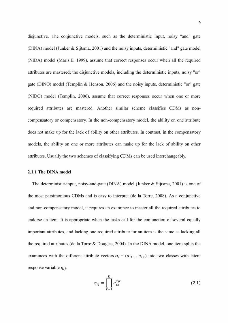
disjunctive. The conjunctive models, such as the deterministic input, noisy "and" gate

(DINA) model (Junker & Sijtsma, 2001) and the noisy inputs, deterministic "and" gate model

(NIDA) model (Maris.E, 1999), assume that correct responses occur when all the required

attributes are mastered; the disjunctive models, including the deterministic inputs, noisy "or"

gate (DINO) model (Templin & Henson, 2006) and the noisy inputs, deterministic "or" gate

(NIDO) model (Templin, 2006), assume that correct responses occur when one or more

required attributes are mastered. Another similar scheme classifies CDMs as non-

compensatory or compensatory. In the non-compensatory model, the ability on one attribute

does not make up for the lack of ability on other attributes. In contrast, in the compensatory

models, the ability on one or more attributes can make up for the lack of ability on other

attributes. Usually the two schemes of classifying CDMs can be used interchangeably.

2.1.1 The DINA model

The deterministic-input, noisy-and-gate (DINA) model (Junker & Sijtsma, 2001) is one of

the most parsimonious CDMs and is easy to interpret (de la Torre, 2008). As a conjunctive

and non-compensatory model, it requires an examinee to master all the required attributes to

endorse an item. It is appropriate when the tasks call for the conjunction of several equally

important attributes, and lacking one required attribute for an item is the same as lacking all

the required attributes (de la Torre & Douglas, 2004). In the DINA model, one item splits the

examinees with the different attribute vectors 𝜶𝒊 = (𝛼𝑖1… 𝛼𝑖𝐾) into two classes with latent

response variable 𝜂𝑖𝑗.

𝜂𝑖𝑗 =∏𝛼𝑖𝑘

𝑞𝑗𝑘

𝐾

𝑘=1

(2.1)

10

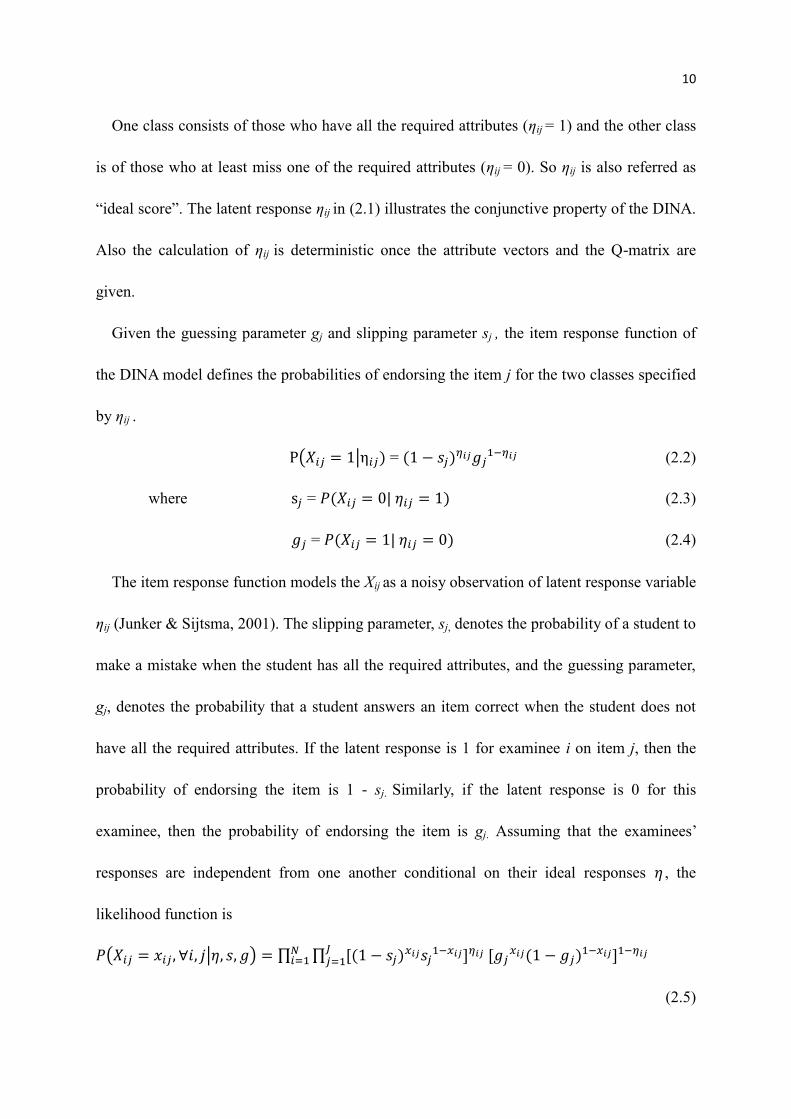
One class consists of those who have all the required attributes (ηij = 1) and the other class

is of those who at least miss one of the required attributes (ηij = 0). So ηij is also referred as

“ideal score”. The latent response ηij in (2.1) illustrates the conjunctive property of the DINA.

Also the calculation of ηij is deterministic once the attribute vectors and the Q-matrix are

given.

Given the guessing parameter gj and slipping parameter sj , the item response function of

the DINA model defines the probabilities of endorsing the item j for the two classes specified

by ηij .

P(𝑋𝑖𝑗 = 1|η𝑖𝑗) = (1 − 𝑠𝑗)𝜂𝑖𝑗𝑔𝑗

1−𝜂𝑖𝑗 (2.2)

where s𝑗 = 𝑃(𝑋𝑖𝑗 = 0| 𝜂𝑖𝑗 = 1) (2.3)

𝑔𝑗 = 𝑃(𝑋𝑖𝑗 = 1| 𝜂𝑖𝑗 = 0) (2.4)

The item response function models the Xij as a noisy observation of latent response variable

ηij (Junker & Sijtsma, 2001). The slipping parameter, sj, denotes the probability of a student to

make a mistake when the student has all the required attributes, and the guessing parameter,

gj, denotes the probability that a student answers an item correct when the student does not

have all the required attributes. If the latent response is 1 for examinee i on item j, then the

probability of endorsing the item is 1 - sj. Similarly, if the latent response is 0 for this

examinee, then the probability of endorsing the item is gj. Assuming that the examinees’

responses are independent from one another conditional on their ideal responses 𝜂 , the

likelihood function is

𝑃(𝑋𝑖𝑗 = 𝑥𝑖𝑗 , ∀𝑖, 𝑗|𝜂, 𝑠, 𝑔) = ∏ ∏ [(1 − 𝑠𝑗)𝑥𝑖𝑗𝑠𝑗

1−𝑥𝑖𝑗]𝜂𝑖𝑗 [𝑔𝑗𝑥𝑖𝑗(1 − 𝑔𝑗)

1−𝑥𝑖𝑗]1−𝜂𝑖𝑗𝐽𝑗=1

𝑁𝑖=1

(2.5)

11

Although the number of required attributes may differ from item to item, the DINA model

requires only two parameters for each item. This is mainly because the strong assumption of

the DINA model that missing one attribute is equivalent to missing all of them. It would be

reasonable to assume an examinee with more but not all required attributes may have a better

chance to guess correct answer than an examinee mastering less attributes does. However, in

the DINA model the guessing and slipping parameters are of item level instead of individual

level.

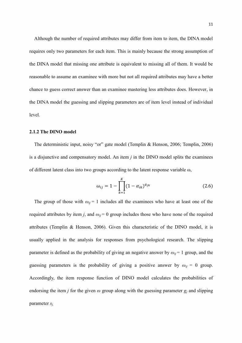
2.1.2 The DINO model

The deterministic input, noisy “or” gate model (Templin & Henson, 2006; Templin, 2006)

is a disjunctive and compensatory model. An item j in the DINO model splits the examinees

of different latent class into two groups according to the latent response variable ω,

ω𝑖𝑗 = 1 −∏(1 − 𝛼𝑖𝑘)𝑞𝑗𝑘 (2.6)

𝐾

𝑘=1

The group of those with ωij = 1 includes all the examinees who have at least one of the

required attributes by item j, and ωij = 0 group includes those who have none of the required

attributes (Templin & Henson, 2006). Given this characteristic of the DINO model, it is

usually applied in the analysis for responses from psychological research. The slipping

parameter is defined as the probability of giving an negative answer by ωij = 1 group, and the

guessing parameters is the probability of giving a positive answer by ωij = 0 group.

Accordingly, the item response function of DINO model calculates the probabilities of

endorsing the item j for the given ω group along with the guessing parameter gj and slipping

parameter sj.

12

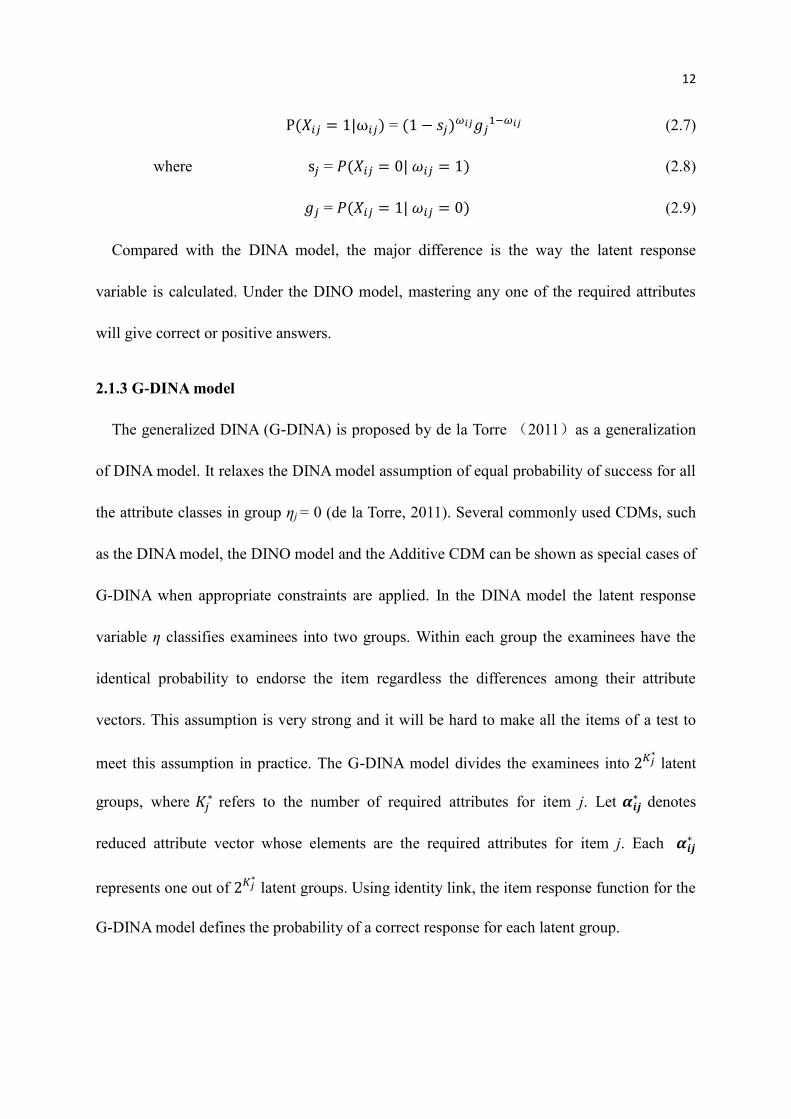
P(𝑋𝑖𝑗 = 1|ω𝑖𝑗) = (1 − 𝑠𝑗)𝜔𝑖𝑗𝑔𝑗

1−𝜔𝑖𝑗 (2.7)

where s𝑗 = 𝑃(𝑋𝑖𝑗 = 0| 𝜔𝑖𝑗 = 1) (2.8)

𝑔𝑗 = 𝑃(𝑋𝑖𝑗 = 1| 𝜔𝑖𝑗 = 0) (2.9)

Compared with the DINA model, the major difference is the way the latent response

variable is calculated. Under the DINO model, mastering any one of the required attributes

will give correct or positive answers.

2.1.3 G-DINA model

The generalized DINA (G-DINA) is proposed by de la Torre （2011）as a generalization

of DINA model. It relaxes the DINA model assumption of equal probability of success for all

the attribute classes in group ηj = 0 (de la Torre, 2011). Several commonly used CDMs, such

as the DINA model, the DINO model and the Additive CDM can be shown as special cases of

G-DINA when appropriate constraints are applied. In the DINA model the latent response

variable η classifies examinees into two groups. Within each group the examinees have the

identical probability to endorse the item regardless the differences among their attribute

vectors. This assumption is very strong and it will be hard to make all the items of a test to

meet this assumption in practice. The G-DINA model divides the examinees into 2𝐾𝑗∗

latent

groups, where 𝐾𝑗∗ refers to the number of required attributes for item j. Let 𝜶𝒊𝒋

∗ denotes

reduced attribute vector whose elements are the required attributes for item j. Each 𝜶𝒊𝒋∗

represents one out of 2𝐾𝑗∗

latent groups. Using identity link, the item response function for the

G-DINA model defines the probability of a correct response for each latent group.

13

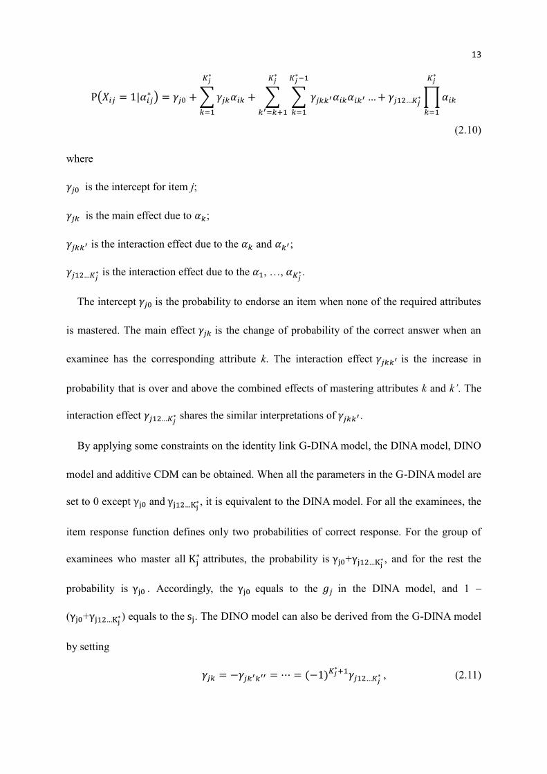
P(𝑋𝑖𝑗 = 1|𝛼𝑖𝑗∗ ) = 𝛾𝑗0 +∑𝛾𝑗𝑘𝛼𝑖𝑘 + ∑ ∑ 𝛾𝑗𝑘𝑘′𝛼𝑖𝑘𝛼𝑖𝑘′

𝐾𝑗∗−1

𝑘=1

𝐾𝑗∗

𝑘′=𝑘+1

𝐾𝑗∗

𝑘=1

…+ 𝛾𝑗12…𝐾𝑗∗∏𝛼𝑖𝑘

𝐾𝑗∗

𝑘=1

(2.10)

where

𝛾𝑗0 is the intercept for item j;

𝛾𝑗𝑘 is the main effect due to 𝛼𝑘;

𝛾𝑗𝑘𝑘′ is the interaction effect due to the 𝛼𝑘 and 𝛼𝑘′;

𝛾𝑗12…𝐾𝑗∗ is the interaction effect due to the 𝛼1, …, 𝛼𝐾𝑗

∗.

The intercept 𝛾𝑗0 is the probability to endorse an item when none of the required attributes

is mastered. The main effect 𝛾𝑗𝑘 is the change of probability of the correct answer when an

examinee has the corresponding attribute k. The interaction effect 𝛾𝑗𝑘𝑘′ is the increase in

probability that is over and above the combined effects of mastering attributes k and k’. The

interaction effect 𝛾𝑗12…𝐾𝑗∗ shares the similar interpretations of 𝛾𝑗𝑘𝑘′.

By applying some constraints on the identity link G-DINA model, the DINA model, DINO

model and additive CDM can be obtained. When all the parameters in the G-DINA model are

set to 0 except γj0 and γj12…Kj∗, it is equivalent to the DINA model. For all the examinees, the

item response function defines only two probabilities of correct response. For the group of

examinees who master all Kj∗ attributes, the probability is γj0+γj12…Kj

∗ , and for the rest the

probability is γj0 . Accordingly, the γj0 equals to the 𝑔𝑗 in the DINA model, and 1 –

(γj0+γj12…Kj∗) equals to the sj. The DINO model can also be derived from the G-DINA model

by setting

𝛾𝑗𝑘 = −𝛾𝑗𝑘′𝑘′′ = ⋯ = (−1)𝐾𝑗∗+1𝛾𝑗12…𝐾𝑗

∗ , (2.11)

14

for k = 1,…, 𝐾𝑗∗ , 𝑘′= 1,…, 𝐾𝑗

∗ -1, and 𝑘′′> 𝑘′ ,…, 𝐾𝑗∗ . Under such setting the guessing

parameter 𝑔𝑗′ was estimated with 𝛿𝑗0 , and that the 1-𝑠𝑗

′ is estimated with 𝛾𝑗0+𝛾𝑗𝑘 for each

item. The probability of correct response for the group with none of the required attributes

is 𝑔𝑗′ , and the probability to endorse the item for the group with at least one of the required

attributes is 1-𝑠𝑗′. If all interaction terms in the G-DINA model are set to be 0, the item

response function is identical to the additive CDM (A-CDM).

2.2 Q-Matrix Diagnostics and Estimation

The item to attribute relationship is crucial in the application for the CDMs, and efforts

have been made on the Q-matrix estimation (Chen, Liu, Xu and Ying, 2015; Chen, Liu and

Ying, 2015; Chung, 2013; Chiu and Douglas, 2013; DeCarlo, 2012; de la Torre, 2008; Liu,

Xu and Ying, 2012; Liu, Xu and Ying, 2013). Some of the studies are introduced in this

section. This section also includes several studies of the effects resulted from using a Q-

matrix that is not appropriately specified.

2.2.1 Estimation of Q-matrix

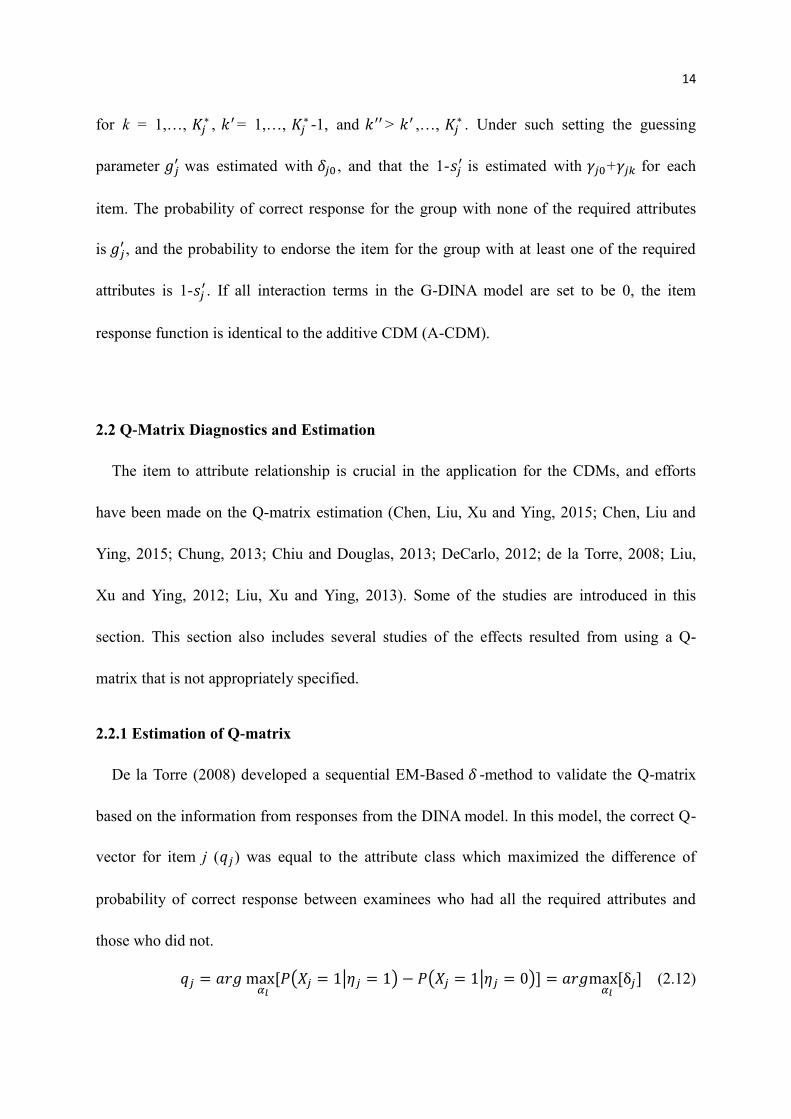
De la Torre (2008) developed a sequential EM-Based 𝛿 -method to validate the Q-matrix

based on the information from responses from the DINA model. In this model, the correct Q-

vector for item j (𝑞𝑗) was equal to the attribute class which maximized the difference of

probability of correct response between examinees who had all the required attributes and

those who did not.

𝑞𝑗 = 𝑎𝑟𝑔 max 𝛼𝑙

[𝑃(𝑋𝑗 = 1|𝜂𝑗 = 1) − 𝑃(𝑋𝑗 = 1|𝜂𝑗 = 0)] = 𝑎𝑟𝑔max 𝛼𝑙

[δ𝑗] (2.12)

15

The equation is equivalent to minimizing the sum of the slipping and guessing parameter 𝑠𝑗

and 𝑔𝑗 of item j given the data. Thus by selecting the optimal q vector, the proposed method

can improve the model fit, and provide information to re-evaluate the Q-matrix. The results

of the simulation study indicated that the proposed method was able to identify and correctly

replace the inappropriate q vectors, while at the same time retain those which were correctly

specified, at least for the conditions in the investigated simulation studies.

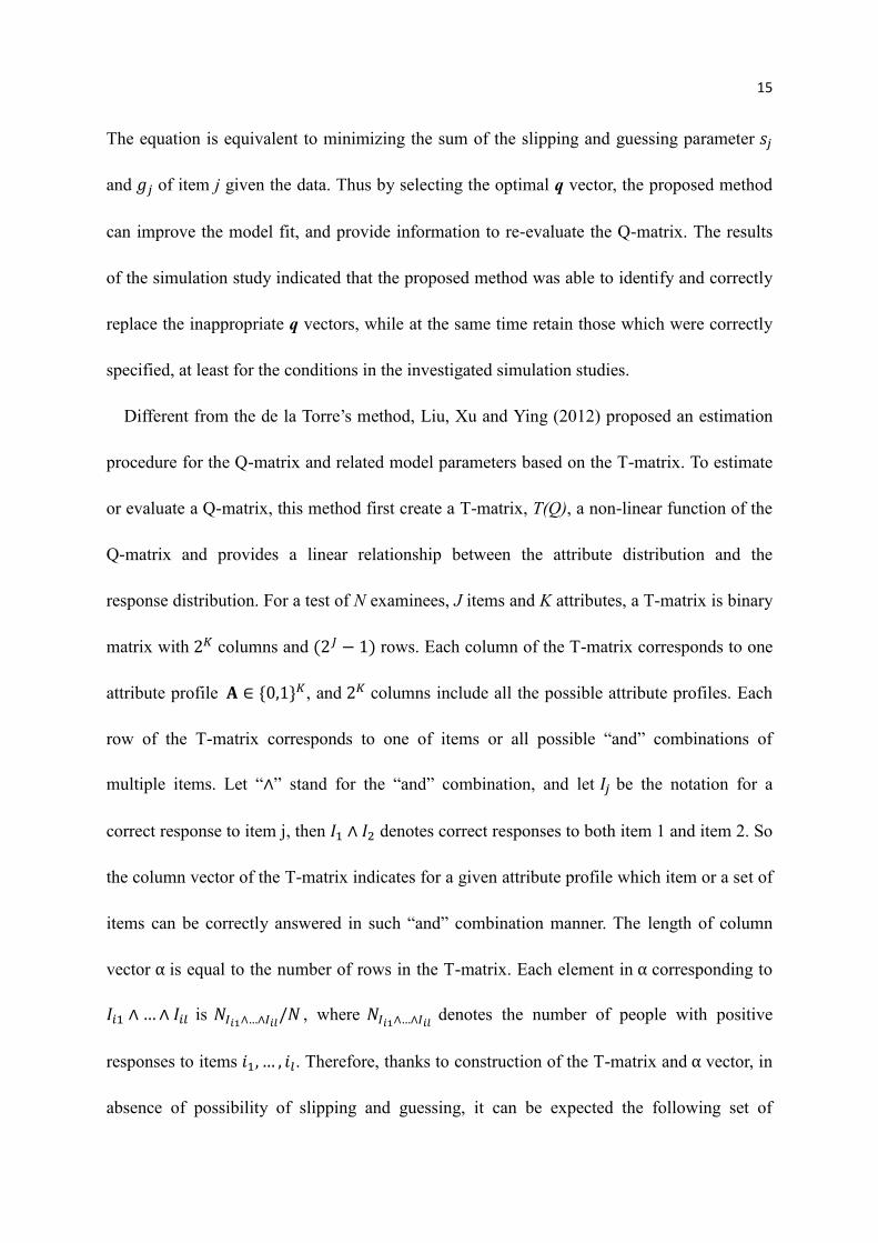
Different from the de la Torre’s method, Liu, Xu and Ying (2012) proposed an estimation

procedure for the Q-matrix and related model parameters based on the T-matrix. To estimate

or evaluate a Q-matrix, this method first create a T-matrix, T(Q), a non-linear function of the

Q-matrix and provides a linear relationship between the attribute distribution and the

response distribution. For a test of N examinees, J items and K attributes, a T-matrix is binary

matrix with 2𝐾 columns and (2𝐽 − 1) rows. Each column of the T-matrix corresponds to one

attribute profile 𝐀 ∈ {0,1}𝐾, and 2𝐾 columns include all the possible attribute profiles. Each

row of the T-matrix corresponds to one of items or all possible “and” combinations of

multiple items. Let “∧” stand for the “and” combination, and let 𝐼𝑗 be the notation for a

correct response to item j, then 𝐼1 ∧ 𝐼2 denotes correct responses to both item 1 and item 2. So

the column vector of the T-matrix indicates for a given attribute profile which item or a set of

items can be correctly answered in such “and” combination manner. The length of column

vector α is equal to the number of rows in the T-matrix. Each element in α corresponding to

𝐼𝑖1 ∧ …∧ 𝐼𝑖𝑙 is 𝑁𝐼𝑖1∧…∧𝐼𝑖𝑙/𝑁 , where 𝑁𝐼𝑖1∧…∧𝐼𝑖𝑙 denotes the number of people with positive

responses to items 𝑖1, … , 𝑖𝑙. Therefore, thanks to construction of the T-matrix and α vector, in

absence of possibility of slipping and guessing, it can be expected the following set of

16

equations

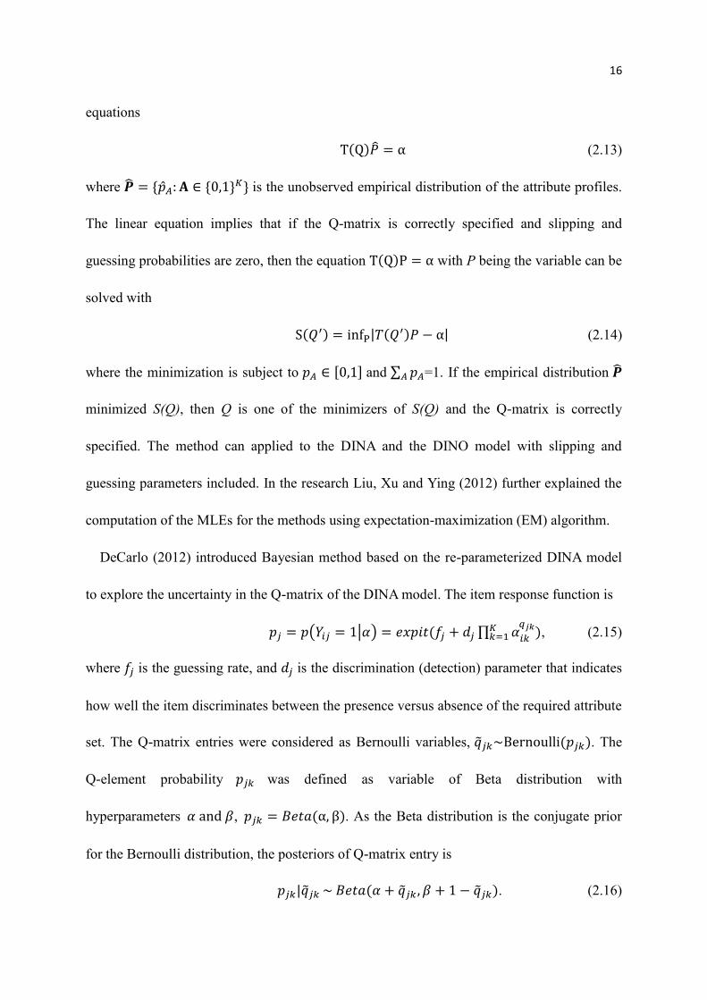
T(Q)�̂� = α (2.13)

where �̂� = {�̂�𝐴: 𝐀 ∈ {0,1}𝐾} is the unobserved empirical distribution of the attribute profiles.

The linear equation implies that if the Q-matrix is correctly specified and slipping and

guessing probabilities are zero, then the equation T(Q)P = α with P being the variable can be

solved with

S(𝑄′) = infP|𝑇(𝑄′)𝑃 − α| (2.14)

where the minimization is subject to 𝑝𝐴 ∈ [0,1] and ∑ 𝑝𝐴𝐴 =1. If the empirical distribution �̂�

minimized S(Q), then Q is one of the minimizers of S(Q) and the Q-matrix is correctly

specified. The method can applied to the DINA and the DINO model with slipping and

guessing parameters included. In the research Liu, Xu and Ying (2012) further explained the

computation of the MLEs for the methods using expectation-maximization (EM) algorithm.

DeCarlo (2012) introduced Bayesian method based on the re-parameterized DINA model

to explore the uncertainty in the Q-matrix of the DINA model. The item response function is

𝑝𝑗 = 𝑝(𝑌𝑖𝑗 = 1|𝛼) = 𝑒𝑥𝑝𝑖𝑡(𝑓𝑗 + 𝑑𝑗∏ 𝛼𝑖𝑘

𝑞𝑗𝑘𝐾𝑘=1 ), (2.15)

where 𝑓𝑗 is the guessing rate, and 𝑑𝑗 is the discrimination (detection) parameter that indicates

how well the item discriminates between the presence versus absence of the required attribute

set. The Q-matrix entries were considered as Bernoulli variables, �̃�𝑗𝑘~Bernoulli(𝑝𝑗𝑘). The

Q-element probability 𝑝𝑗𝑘 was defined as variable of Beta distribution with

hyperparameters 𝛼 and 𝛽, 𝑝𝑗𝑘 = 𝐵𝑒𝑡𝑎(α, β). As the Beta distribution is the conjugate prior

for the Bernoulli distribution, the posteriors of Q-matrix entry is

𝑝𝑗𝑘|�̃�𝑗𝑘 ~ 𝐵𝑒𝑡𝑎(𝛼 + �̃�𝑗𝑘 , 𝛽 + 1 − �̃�𝑗𝑘). (2.16)

17

The simulations of the study showed that the posterior distributions for the random Q-matrix

elements provided useful information about which elements should be or should not be

included. The method recovered uncertain elements of the Q-matrix quite well in a number of

simulation conditions with the rest of the elements correctly specified. Given that Bayesian

version of the re-parameterized DINA model was able to estimate some elements of the Q-

matrix, Bayesian method may have the potential to estimate the entire Q-matrix. Moreover,

the Q-matrix estimation is a task to find the Q-matrix, item statistics and attribute classes of

examinees that fits the observed data best. The number of parameters is large and the

parameter space may be non-convex. Thus Bayesian method is adopted in the present paper

for the Q-matrix estimation.

Chung (2013) also worked on the Q-matrix estimation in Bayesian frame for his

dissertation. The MCMC algorithm was used for Q-matrix estimation. A saturated

multinomial model was used to estimate correlated attributes in the DINA model and rRUM.

Closed-forms of posteriors for guess and slip parameters were derived for the DINA model.

The random walk Metropolis-Hastings algorithm was applied to parameter estimation in the

rRUM.

Chiu and Douglas (2013) introduced a nonparametric classification method that only

requires specification of an item-by-attribute association matrix, and the classifiers according

to minimizing a distance measure between observed responses, and the ideal response for a

given attribute profile that would be implied by the item-by-attribute association matrix. To

refine the estimated Q-matrix, Chiu (2013) developed method for identifying and correcting

the miss-specified q-entries of a Q-matrix. The method operates by minimizing the residual

18

sum of squares (RSS) between the observed responses and the ideal responses to a test item.

The algorithm begins by targeting the item with the highest RSS and determining whether its

q-vector should be updated. It may not be clear, whether a high RSS is due to a miss-

specified q-vector or to examinee misclassification, or is just inherently high (e.g., because of

random error). If the RSS is inherently high, it can happen that the RSS for the item remains

high even after that item has been evaluated, which will prevent the algorithm from

continuing. To avoid revisiting an item with a high RSS but a correctly specified q-vector, the

algorithm visits each item only once until all items have been evaluated. Because examinees

are reclassified with every update of the Q-matrix, the RSS of each item decreases as the

algorithm continues. Each update to the Q-matrix may provide new information that allows

additional updates to the q-vectors, even those for items that have already been evaluated.

Therefore, all items must usually be visited several times until the stopping criterion is met.

2.2.2 Diagnostics of Q-Matrix

Rupp and Templin (2008) investigated the effect of the Q-matrix misspecification on

parameter estimation for the DINA model. The study used a Q-matrix of 15 possible attribute

patterns based on four independent attributes. For each item, one of the entries in the Q-

matrix was misspecified. The research showed the evidences that the slipping parameters for

a misspecified item is overestimated when attributes are incorrectly omitted in the Q-matrix.

In contrast, when an unnecessary attributes are added in the Q-matrix for a particular item,

the guessing parameters for the misspecified item is overestimated most strongly. The study

also indicated high misclassification rates for attribute classes that contained attribute

19

combinations that were deleted from the Q-matrix.

Im and Corter (2011) studied the statistical consequences of attribute misspecification in

the rule space model for cognitively diagnostic measurement.. The results support the

following conclusions. First, when an essential attribute was excluded, the classification

consistencies of examinees’ attribute mastery were lower than the consistencies when

superfluous attribute is included. In other words, inclusion of the superfluous attribute was

less influential to the reclassified examinees. Second, when an essential attribute was

excluded, the attribute mastery probability was underestimated. Third, when an essential

attribute is excluded, the root mean square errors of the estimated attribute mastery

probabilities were larger than the root mean squares when a superfluous attribute is included.

DeCarlo (2011) analyzed fraction subtraction data of Tatsuoka (1990) with the DINA

model and the revealed problems with respect to the classification of examinees. The

problems included that examinees that get all of the items incorrect are classified as having

most of the skills; and that obtaining large estimates of the latent class sizes can indicate

misspecification of the Q-matrix. It was shown that the revealed problems were largely

associated with the structure of the Q-matrix. The simulation with particular Q-matrix under

question was suggested to provide information about the sensitivity of the classifications.

2.3 Bayesian statistics

Bayesian statistic is a branch of statistics that applies Bayes’ rule to solve inferential

questions of interest. In practice Bayesian methods present alternatives that often allow for

20

more intricate models to be fit to complex data. The advances in computing inspire the

growth of Bayesian inference in recent years. Multi-dimensional integrals often arise in

Bayesian statistics, so MCMC methods are usually used. This section briefly reviews

Bayesian statistics and the MCMC method that are relative to the present study.

Bayesian statistical methods are used to compute probability distributions of parameters in

statistical models, based on data and the previous knowledge about the parameters. Let 𝜽

denotes the unknown parameters and X represents the data. For the point or interval estimate

of a parameter 𝜃 in a model based on data X, the posterior distribution of the parameter is

𝑃(𝜃|𝑿) =𝑃(𝑿|𝜃)𝑃(𝜃)

𝑃(𝑿)=

𝑃(𝑿|𝜃)𝑃(𝜃)

∫𝑃(𝑿|𝜃)𝑃(𝜃)𝑑𝜃 , (2.17)

where 𝑃(𝜃) is the prior density for the parameter and 𝑃(𝑿|𝜃) is the likelihood function. In

Bayesian inference, the prior distribution incorporates the subjective beliefs about the

parameters. If the prior information about the parameter is not available, an uninformative (or

vague) prior is usually assigned. The prior distribution is updated with the likelihood function

using Bayes’ theorem to obtain the posterior distribution. The posterior distribution is the

probability distribution that represents the updated beliefs about the parameter after seeing

the data. If the prior is uninformative, the posterior is very much determined by the data; if

the prior is informative, the posterior is mixture of the prior and the data; the more

informative the prior, the more data is needed to change the initial beliefs; for the data set that

is large enough, the data will dominate the posterior distribution. The denominator 𝑃(𝑿) is

the marginal likelihood of 𝑿 and it is generally difficult to calculate ∫𝑃(𝑿|𝜃)𝑃(𝜃)𝑑𝜃 in a

closed-form. It rescales 𝑃(𝑿|𝜃)𝑃(𝜃) computations to be measured as a proper probabilities,

i.e., the posterior distribution will integrate or sum to 1. Without the rescaling, 𝑃(𝑋|𝜃)𝑃(𝜃) is

21

still a valid relative measure of 𝑃(𝜃|𝑋) , but are not restricted to the [0,1] interval.

Accordingly 𝑃(𝑋) is often left out and Posterior ∝ Prior × Likelihood.

Conjugate distributions are those whose prior and posterior distributions are the same, and

in such case the prior is called the conjugate prior. It is favored for its algebraic conveniences,

especially when the likelihood has a distribution in the form of exponential family, such as

the Gaussian distribution or the Beta distribution. For example, the beta distribution is the

conjugate family for the binomial likelihood. Suppose 𝑦 is a sequence of n independent

Bernoulli variables with success probability 𝑝 ∈ [0,1], and x is the number of success, then

𝑓 (x|n, p) = (𝑛𝑥)𝑝𝑥(1 − 𝑝)𝑛−𝑥 (2.18)

Let p follows the Beta distribution with the parameter 𝛼 and 𝛽, Beta(p; α, β)

Beta(p; α, β) =𝛤(𝛼+𝛽)

𝛤(𝛼)𝛤(𝛽)𝑝𝛼−1(1 − 𝑝)𝛽−1 =

1

𝐵(𝛼,𝛽)𝑝𝛼−1(1 − 𝑝)𝛽−1 (2.19)

where the Gamma function 𝛤(𝑥) is the generalization of the factorial x! to the reals

Γ(α)=∫ 𝑥𝛼−1𝑒−𝑥𝑑𝑥 𝑓𝑜𝑟 ∞

0 𝛼 > 0 (2.20)

The Beta function 𝐵(𝛼, 𝛽) is a normalizing constant. Then the posterior distribution

𝑓 (𝑝 |𝑦 ) ∝

𝑛!

𝑥!(𝑛−𝑥)!

𝛤(𝛼+𝛽)

𝛤(𝛼)𝛤(𝛽)𝑝𝛼+𝑥−1(1 − 𝑝)𝛽+𝑛−𝑥−1 (2.21)

which is the Beta distribution with parameter (𝑎 + 𝑥 ) and (𝑏 + 𝑛 − 𝑥 ).

Conjugate analyses are convenient and especially beneficial when carrying posterior

simulations using Gibbs sampling. However the conjugate prior is not always available in

practice. In most of the cases, the posterior distribution has to be found numerically via

simulation.

In Bayesian data analysis, the integration is the principle inferential operation. Historically

the need to evaluate the integrals was a major difficulty for the using Bayesian methods. After

22

the MCMC methods (Gelfand & Smith, 1990) were popularized as the computing resources

became widely available, the Markov chains were used in various situations including

Bayesian data analysis.

2.4 Markov chain Monte Carlo methods

A Monte Carlo approach relies on repeated random sampling to obtain numerical results. A

Markov chain is a sequence 𝑥(1), … , 𝑥(𝑘) such that for each j, 𝑥(𝑗+1) follow the

distribution 𝑝 (𝑥|𝑥(𝑗)), which only depends on 𝑥(𝑗). This conditional probability distribution

is called a transition kernel. In statistics MCMC methods are a class of algorithms for

sampling from probability distributions based on constructing a Markov chain that has the

desired distribution as its equilibrium distribution. The state of the chain after a sufficient

number of steps is then used as a sample of the desired distribution. Essentially the MCMC

methods are not optimization techniques, but random number generation methods. However

they are often applied to solve optimization problems in large dimensional spaces (Andrieu,

De Freitas, Doucet, & Jordan, 2004).

The Metropolis-Hastings algorithms (Metropolis, 1953; Hastings, 1970) generate the

Markov chains which converge to desired distribution by successively sampling from an

essentially arbitrary transition kernel, and imposing a random rejection step at each transition.

As more and more sample values are produced, the distribution of values more closely

approximates the desired distribution. The sample values are produced iteratively. The

algorithm picks a candidate for the next sample value based on the sampled value from

23

current iteration. Then with some probability the candidate is either accepted or rejected. The

probability of acceptance is determined by comparing the likelihoods of the current and the

candidate sample values with respect to the desired distribution. Let 𝑓(𝑥) and 𝑞(𝑥|𝑥∗) denote

the desired distribution and proposal distribution respectively. The Metropolis-Hastings

algorithm entails simulating 𝑥(1), … , 𝑥(𝑘) by iterating two steps: (1) given point 𝑥(𝑡) ,

generate 𝑌𝑡~𝑞(𝑦|𝑥(𝑡)), (2) take

𝑋(𝑡+1) = {𝑌𝑡 𝑤𝑖𝑡ℎ 𝑝𝑟𝑜𝑏𝑎𝑏𝑖𝑙𝑖𝑡𝑦 𝜌(𝑥

(𝑡), 𝑌𝑡),

𝑥(𝑡) 𝑤𝑖𝑡ℎ 𝑝𝑟𝑜𝑏𝑎𝑏𝑖𝑙𝑖𝑡𝑦 1 − 𝜌(𝑥(𝑡), 𝑌𝑡), (2.22)

where ρ(𝑥, 𝑦 ) = min {1,𝑓(𝑦)

𝑓(𝑥)

𝑞(𝑥|𝑦)

𝑞(𝑦|𝑥)}.

The ρ(𝑥, 𝑦 ) denotes the acceptance probability, which basically accept a proposal point

that increases the probability, and sometimes accept one that does not. The independent

sampler and Metropolis algorithm are two simple instances of the Metropolis-Hastings

algorithm (Andrieu et al., 2004). In the independent sampler the proposal is independent of

the current state, 𝑞(𝑦|𝑥(𝑡)) = 𝑞(𝑦). Hence the acceptance probability is min {1,𝑓(𝑦)

𝑓(𝑥)

𝑞(𝑥)

𝑞(𝑦)}.

The Metropolis algorithm assumes a symmetric random walk proposal 𝑞(𝑦|𝒙(𝑡)) = 𝑞(𝒙(𝑡)|y)

and the acceptance ration simplifies to min {1,𝑓(𝑦)

𝑓(𝑥)}.

Gibbs sampling (Geman & Geman, 1984) is a generalized probabilistic inference algorithm

to generate a sequence of samples from a joint probability distribution 𝑝 (𝒙) of two or more

random variables (Casella & George, 1992). Gibbs sampling is a variation of the Metropolis-

Hastings algorithm and the power of this algorithm is that the sampling joint distribution of

the variables will converge to the joint probability of the variables and the acceptance rate for

each sampling is 1. Gibbs sampling is obtained when adopt the full conditional distributions

24

𝑝 (𝑥𝑗|𝒙−𝑗) = 𝑝(𝑥𝑗|𝑥1…𝑥𝑗−1, 𝑥𝑗+1, … , 𝑥𝑛) as the proposal distributions. A full conditional

distribution is a normalized distribution that allows the sampling along one coordinate

direction. With an initial starting point for the joint probability distribution, a value for one

dimension is sampled given values of other dimensions. Within the iteration, the sampling

goes through all the dimensions one at a time, which gives a sample of joint probability

distribution. Specifically the proposal distribution 𝑞(𝑦𝑗|𝒙(𝑡)) = 𝑝 (𝑦𝑗|𝒙 −𝑗

(𝑡)) and so for j =

1,…,n

ρ (𝒙, 𝑦𝑗 ) = min {1,𝑝(𝑦𝑗|𝒙 )

𝑝(𝑥𝑗|𝒙 )

𝑞(𝑥𝑗|𝑦𝑗,𝒙−𝑗)

𝑞(𝑦𝑗|𝑥𝑗 , 𝒙−𝑗)}

= min {1,𝑝(𝑦𝑗|𝒙−𝑗)

𝑝(𝑥𝑗|𝒙−𝑗)

𝑝(𝑥𝑗|𝒙−𝑗)

𝑝(𝑦𝑗|𝒙−𝑗)}

= 1 (2.23)

From the theory of Markov chains, it is expected that the chains converge to the stationary

distribution, which is the target distribution. However there is no guarantee that a chain will

converged after a limited number of sampling. Thus it is important in the application of the

MCMC to determine when it is safe to stop sampling.

Diagnostics for MCMC Convergence

The convergence diagnostics of Gelman and Rubin (1992) and Raftery and Lewis (1992)

are currently most popular methods (Cowles & Carlin, 1996). In addition to these two, other

convergence diagnostics research were conducted by Geweke (1992), Johnson (1994), Liu,

Liu & Rubin (1992), Roberts (1995), Yu & Mykland (1994), and Zellner & Min (1995),

Gelman and Rubin Shrink Factor

The Gelman and Rubin’s method is essentially a univariate method. It first estimates the

25

overdispersion and decides the number of independent chains to sample. Let m denotes the

number of chains, then after the sampling of m chains, the within chain variance W and

between chain variance B can be calculated. Slowly-mixing samplers will initially have B

much bigger than W, since the chain starting points are overdispersed relative to the target

density. The estimated variance, E, of the stationary distribution is a weighted average of

within and between chain variance. The potential scale reduction factor is �̂� = √�̂�

𝑊 . The

value approaches one when the pooled within-chain variance dominates the between-chain

variance, and all chains forgot their starting points and have traversed all the target

distribution. Thus when �̂� is high, it may indicate that a larger number of sampling is needed

to improve convergence to the stationary distribution.

However, to apply the shrink factor method, one need to find the starting distribution that

is overdispersed with respect to the target distribution, a condition that requires knowledge of

latter to verify. Further, since Gibbs sampler is most needed when the normal approximation

to the posterior distribution is inadequate for purpose of estimation and inference, reliance on

normal approximation for diagnosing convergence to the true posterior may be questionable

(Cowles & Carlin 1996).

Raftery-Lewis diagnostic

The Raftery-Lewis diagnostic test finds the number of iterations, M, that need to be

discarded (burn-ins) and the number of iterations needed, N, to achieve a desired precision.

Suppose a quantity 𝜃𝑞 is of interest such that𝑃(𝜃 ≤ 𝜃𝑞|𝒙) = 𝑞, where 𝑞 can be an arbitrary

cumulative probability, such as 0.025. This 𝜃𝑞 can be empirically estimated from the

sorted {𝜃𝑡} . Let 𝜃 q denote the estimate?? which corresponds to an estimated probability

26

𝑃(𝜃 ≤ 𝜃 q ) = �̂� q . Because the simulated posterior distribution converges to the true

distribution as the simulation sample size grows, 𝜃q can achieve any degree of accuracy if the

simulator is run for a very long time. However, running too long a simulation can be

wasteful. Alternatively, coverage probability can be used to measure accuracy and stop the

chain when certain accuracy is reached.

A stopping criterion is reached when the estimated probability is within ±𝑟 of the true

cumulative probability 𝑞, with probability 𝑠, such as 𝑃(�̂�q ∈ (𝑞 − 𝑟, 𝑞 + 𝑟)) = 𝑠.

Given a predefined cumulative probability 𝑞, these procedures first find 𝜃q, and then they

construct a binary process {𝑍𝑡} by setting 𝑍𝑡 = 1 if 𝜃𝑡 ≤ 𝜃q and 0 otherwise for all t. The

sequence {𝑍𝑡} is itself not a Markov chain, but the subsequence of {𝑍𝑡} can be constructed as

Markovian if it is sufficiently 𝑘-thinned. When 𝑘 becomes reasonably large, {𝑍𝑡(𝑘)} starts to

behave like a Markov chain.

When k is determined, the transition probability matrix between state 0 and state 1

for {𝑍𝑡(𝑘)} is: 𝑄 = (1−𝛼

𝛽𝛼1−𝛽

). Because {𝑍𝑡(𝑘)} is a Markov chain, its equilibrium distribution

exists and is estimated by 𝜋 = (𝜋0, 𝜋1) =(𝛽,𝛼)

𝛼+𝛽 where 𝜋0 = 𝑃(𝜃 ≤ 𝜃𝑞|𝒙) and 𝜋1 = 1 − 𝜋0 .

The goal is to find an iteration number m such that after m steps, the estimated transition

probability 𝑃(𝑍𝑚(𝑘) = 𝑖|𝑍0

(𝑘) = 𝑗 is within 휀 of equilibrium 𝜇𝑖 for 𝑖, 𝑗 = 0, 1 . Let 𝑒0 =

(1,0) and 𝑒1 = 1 − 𝑒0. The estimated transition probability after step is

P(Zm(k)= i|Z0

(k)= j) = ej [(

π0 π1π0 π1

) +(1−α−β)m

α+β(α −α−β β

)] ej (2.24)

which holds when m =log(

(α+β)ε

max (α,β))

log (1−α−β) assuming 1 − α − β > 0.

Therefore, by time m, {𝑍𝑡(𝑘)} is sufficiently close to its equilibrium distribution, the total

size of 𝑀 = 𝑚𝑘 should be discarded as the burn-in. Next, the procedures estimate N, the

27

number of simulations needed to achieve desired accuracy on percentile estimation. The

estimate of 𝑝(𝜃 ≤ 𝜃𝑞|𝑦) is �̅�𝑡(𝑘)=

1

𝑛∑ 𝑍𝑡

(𝑘)𝑛𝑡=1 . For large n, �̅�𝑡

(𝑘) is normally distributed with

mean q, the true cumulative probability, and variance 1

𝑛

(2−𝛼−𝛽)𝛼𝛽

(𝛼+𝛽)3. 𝑃(𝑞 − 𝑟 ≤ �̅�𝑡

(𝑘) ≤ 𝑞 +

𝑟) = 𝑠 is satisfied if 𝑛 =(2−𝛼−𝛽)𝛼𝛽

(𝛼+𝛽)3(𝛷−1(

𝑠+1

2)

𝑟)

2

. Therefore 𝑁 = 𝑛𝑘

28

Chapter 3

Methods

Some CDMs can be achieved by applying certain constraints on the G-DINA model, which

makes it possible to estimate the Q-matrix empirically for these CDMs models through G-

DINA model. This chapter develops the method to estimate the Q-matrix for the DINA model

using the constrained G-DINA model. The present study adopted Bayesian statistics and

Gibbs sampling for the model parameter estimation. The prior distributions used in analysis

are non-informative. The MCMC estimation procedure may pose problems of label

switching, and the current paper applied the method of Stephens (2000) to relabel the

sampling results. Section 3.1 introduces the model specification, notation and constraints on

G-DINA model. Bayesian formulations and sampling procedures for the Q-matrix estimation

were developed in section 3.2. Section 3.3 shows the relabeling algorithm and finalizing Q-

matrix. Simulation and empirical studies designs are in section 3.4.

3.1 Model specification and Notation

The present paper is concerned with N examinees taking a test of J items for assessing K

attributes of examinees. The response vector of ith

examinee is denoted by Xi, i = 1, 2,…, N.

The response vector contains the observed scores for the J items, and so, Xi = (Xi1,…, Xij,…,

29

XiJ) with the binary entries, where 1 denotes correct and 0 denotes incorrect on the jth

item.

𝑋𝑖𝑗 = { 1 𝑖𝑓 𝑡ℎ𝑒 𝑠𝑢𝑏𝑗𝑒𝑐𝑡 𝑖 𝑎𝑛𝑠𝑤𝑒𝑟𝑠 𝑖𝑡𝑒𝑚 𝑗 𝑐𝑜𝑟𝑟𝑒𝑐𝑡𝑙𝑦

0 𝑖𝑓 𝑡ℎ𝑒 𝑠𝑢𝑏𝑗𝑒𝑐𝑡 𝑖 𝑎𝑛𝑠𝑤𝑒𝑟𝑠 𝑖𝑡𝑒𝑚 𝑗 𝑖𝑛𝑐𝑜𝑟𝑟𝑒𝑐𝑡𝑙𝑦

The G-DINA model takes N×J binary response matrix X as input. The attribute vector of

ith

examinee is denoted by αi= (αi1,…αik,…,αiK) with binary entries, where αik = 1 means that

the ith

examinee masters the attribute k and 0 denotes non-mastery.

𝛼𝑖𝑘 = { 1 𝑖𝑓 𝑡ℎ𝑒 𝑠𝑢𝑏𝑗𝑒𝑐𝑡 𝑖 𝑚𝑎𝑠𝑡𝑒𝑟𝑠 𝑎𝑡𝑡𝑟𝑖𝑏𝑢𝑡𝑒 𝑘

0 𝑖𝑓 𝑡ℎ𝑒 𝑠𝑢𝑏𝑗𝑒𝑐𝑡 𝑖 𝑑𝑜𝑒𝑠 𝑛𝑜𝑡 𝑚𝑎𝑠𝑡𝑒𝑟 𝑎𝑡𝑡𝑟𝑖𝑏𝑢𝑡𝑒 𝑘

Note that the attribute vector is latent, so it cannot be observed. In addition, the G-DINA

model requires a J×K binary Q-matrix as input. It indicates which attributes are required for

each item. For each j and k, qjk equals to 1 indicates that the item j requires the attribute k, and

qjk equals to 0 indicates otherwise.

𝑞𝑗𝑘 = { 1 𝑖𝑓 𝑡ℎ𝑒 𝑖𝑡𝑒𝑚 𝑗 𝑟𝑒𝑞𝑢𝑟𝑖𝑒𝑠 𝑡ℎ𝑒 𝑎𝑡𝑡𝑟𝑖𝑏𝑢𝑡𝑒 𝑘 0 𝑖𝑓 𝑡ℎ𝑒 𝑖𝑡𝑒𝑚 𝑗 𝑑𝑜𝑒𝑠 𝑛𝑜𝑡 𝑟𝑒𝑞𝑢𝑖𝑟𝑒 𝑡ℎ𝑒 𝑎𝑡𝑡𝑟𝑖𝑏𝑢𝑡 𝑘

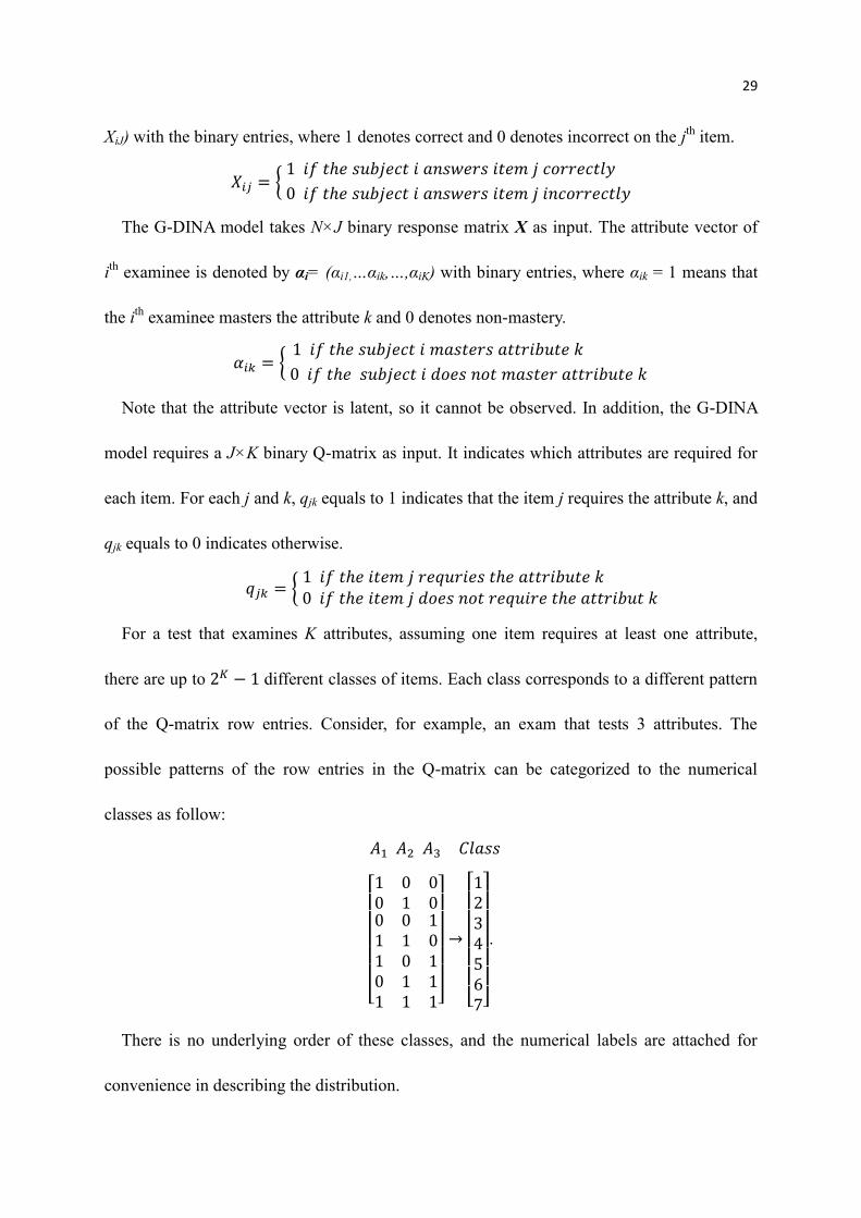
For a test that examines K attributes, assuming one item requires at least one attribute,

there are up to 2𝐾 − 1 different classes of items. Each class corresponds to a different pattern

of the Q-matrix row entries. Consider, for example, an exam that tests 3 attributes. The

possible patterns of the row entries in the Q-matrix can be categorized to the numerical

classes as follow:

𝐴1 𝐴2 𝐴3 𝐶𝑙𝑎𝑠𝑠

[

1 0 00 1 00 0 11 1 01 0 10 1 11 1 1]

→

[

1234567]

.

There is no underlying order of these classes, and the numerical labels are attached for

convenience in describing the distribution.

30

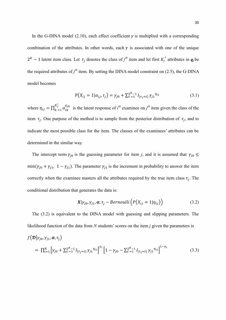
In the G-DINA model (2.10), each effect coefficient 𝛾 is multiplied with a corresponding

combination of the attributes. In other words, each 𝛾 is associated with one of the unique

2𝐾 − 1 latent item class. Let 𝜏𝑗 denotes the class of j

th item and let first Kj

* attributes in qj be

the required attributes of jth

item. By setting the DINA model constraint on (2.5), the G-DINA

model becomes

P(𝑋𝑖𝑗 = 1|𝛼𝑖𝑗 , 𝜏𝑗

) = 𝛾𝑗0 + ∑ 𝐼{𝜏𝑗=𝑡}2𝐾−1𝑡 =1 𝛾𝑗1

𝜂𝑖𝑗 (3.1)

where 𝜂𝑖𝑗 = ∏ 𝛼𝑖𝑘 𝑞𝑗𝑘 𝐾𝑗

∗

𝑘 =1 is the latent response of ith

examinee on jth

item given the class of the

item 𝜏𝑗 . One purpose of the method is to sample from the posterior distribution of 𝜏𝑗, and to

indicate the most possible class for the item. The classes of the examinees’ attributes can be

determined in the similar way.

The intercept term 𝛾𝑗0 is the guessing parameter for item j, and it is assumed that 𝛾𝑗0 ≤

min (𝛾𝑗0 + 𝛾𝑗1, 1 − 𝛾𝑗1). The parameter 𝛾𝑗1 is the increment in probability to answer the item

correctly when the examinee masters all the attributes required by the true item class 𝜏𝑗 . The

conditional distribution that generates the data is:

𝑿|𝛾𝑗0, 𝛾𝑗1, 𝜶, 𝜏𝑗 ~ 𝐵𝑒𝑟𝑛𝑜𝑢𝑙𝑙𝑖 (𝑃(𝑋𝑖𝑗 = 1|𝜂𝑖𝑗)) (3.2)

The (3.2) is equivalent to the DINA model with guessing and slipping parameters. The

likelihood function of the data from N students’ scores on the item j given the parameters is

𝑓(𝓓|𝛾𝑗0, 𝛾𝑗1, 𝜶, 𝜏𝑗 )

= ∏ [𝛾𝑗0 + ∑ 𝐼{𝜏𝑗=𝑡}2𝐾−1𝑡 =1 𝛾𝑗1

𝜂𝑖𝑗]𝑦𝑖𝑁

𝑖=1 [1 − 𝛾𝑗0 − ∑ 𝐼{𝜏𝑗=𝑡}2𝐾−1𝑡 =1 𝛾𝑗1

𝜂𝑖𝑗]1−𝑦𝑖

(3.3)

31

3.2 Estimating the Q-matrix

The estimation method developed in the present study assumes that examinees’ true

attribute classes are not available when the examinees’ scores are collected. In this section let

𝜏𝑗 denotes the sampled class for j

th item from previous iteration. The method takes Xi as input,

and samples the 𝜏𝑗 , 𝛾𝑗0 and 𝛾𝑗1 for each item j, and examinees’ attribute class for each

individual. The full conditional distribution of each parameter is derived for Gibbs sampling.

The steps of the algorithm are described in detail.

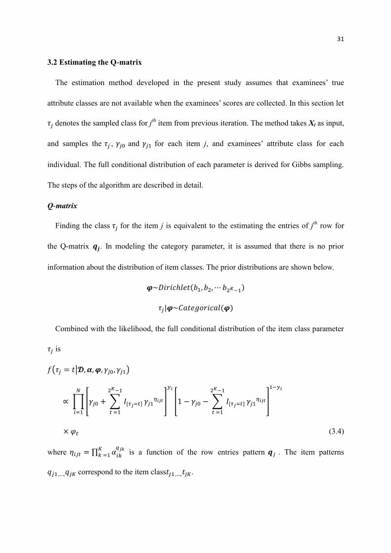
Q-matrix

Finding the class 𝜏𝑗 for the item j is equivalent to the estimating the entries of j

th row for

the Q-matrix 𝒒𝒋. In modeling the category parameter, it is assumed that there is no prior

information about the distribution of item classes. The prior distributions are shown below.

𝝋~𝐷𝑖𝑟𝑖𝑐ℎ𝑙𝑒𝑡(𝑏1, 𝑏2, ⋯ 𝑏2𝐾−1)

𝜏𝑗|𝝋~𝐶𝑎𝑡𝑒𝑔𝑜𝑟𝑖𝑐𝑎𝑙(𝝋)

Combined with the likelihood, the full conditional distribution of the item class parameter

𝜏𝑗 is

𝑓(𝜏𝑗 = 𝑡|𝓓, 𝜶,𝝋, 𝛾𝑗0, 𝛾𝑗1)

∝ ∏[𝛾𝑗0 + ∑ 𝐼{𝜏𝑗=𝑡}

2𝐾−1

𝑡 =1

𝛾𝑗1𝜂𝑖𝑗𝑡]

𝑦𝑖𝑁

𝑖=1

[1 − 𝛾𝑗0 − ∑ 𝐼{𝜏𝑗=𝑡}

2𝐾−1

𝑡 =1

𝛾𝑗1𝜂𝑖𝑗𝑡]

1−𝑦𝑖

× 𝜑𝑡 (3.4)

where 𝜂𝑖𝑗𝑡 = ∏ 𝛼𝑖𝑘 𝑞𝑗𝑘 𝐾

𝑘 =1 is a function of the row entries pattern 𝒒𝑗 . The item patterns

𝑞𝑗1 ,…,𝑞𝑗𝐾 correspond to the item class𝑡𝑗1 ,…,𝑡𝑗𝐾.

32

𝜏𝑗|𝝋~𝐶𝑎𝑡𝑒𝑔𝑜𝑟𝑖𝑐𝑎𝑙 (𝜑𝑡×∏ [𝛾𝑗0+∑ 𝐼{𝜏𝑗=𝑡}

2𝐾−1𝑡 =1 𝛾𝑗1

𝜂𝑖𝑗𝑡]

𝑦𝑖𝑁𝑖=1 [1−𝛾𝑗0−∑ 𝐼{𝜏𝑗=𝑡}

2𝐾−1𝑡 =1 𝛾𝑗1

𝜂𝑖𝑗𝑡]

1−𝑦𝑖

∑ 𝜑𝑡×∏ [𝛾𝑗0+∑ 𝐼{𝜏𝑗=𝑡}2𝐾−1𝑡 =1 𝛾𝑗1

𝜂𝑖𝑗𝑡]

𝑦𝑖𝑁𝑖=1 [1−𝛾𝑗0−∑ 𝐼{𝜏𝑗=𝑡}

2𝐾−1𝑡 =1 𝛾𝑗1

𝜂𝑖𝑗𝑡]

1−𝑦𝑖2𝐾−1𝑡=1

) (3.5)

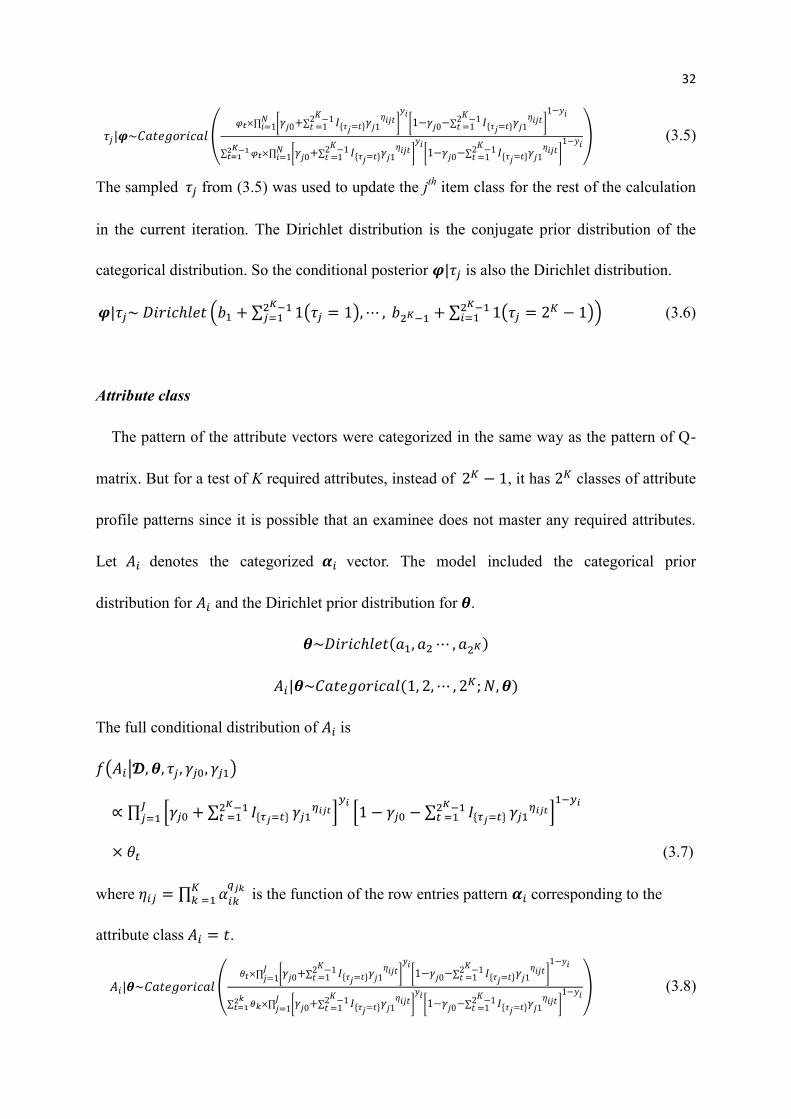
The sampled 𝜏𝑗 from (3.5) was used to update the jth

item class for the rest of the calculation

in the current iteration. The Dirichlet distribution is the conjugate prior distribution of the

categorical distribution. So the conditional posterior 𝝋|𝜏𝑗 is also the Dirichlet distribution.

𝝋|𝜏𝑗~ 𝐷𝑖𝑟𝑖𝑐ℎ𝑙𝑒𝑡 (𝑏1 + ∑ 1(𝜏𝑗 = 1),⋯ ,2𝐾−1𝑗=1 𝑏2𝐾−1 + ∑ 1(𝜏𝑗 = 2

𝐾 − 1)2𝐾−1𝑖=1 ) (3.6)

Attribute class

The pattern of the attribute vectors were categorized in the same way as the pattern of Q-

matrix. But for a test of K required attributes, instead of 2𝐾 − 1, it has 2𝐾 classes of attribute

profile patterns since it is possible that an examinee does not master any required attributes.

Let 𝐴𝑖 denotes the categorized 𝜶𝑖 vector. The model included the categorical prior

distribution for 𝐴𝑖 and the Dirichlet prior distribution for 𝜽.

𝜽~𝐷𝑖𝑟𝑖𝑐ℎ𝑙𝑒𝑡(𝑎1, 𝑎2⋯ , 𝑎2𝐾)

𝐴𝑖|𝜽~𝐶𝑎𝑡𝑒𝑔𝑜𝑟𝑖𝑐𝑎𝑙(1, 2,⋯ , 2𝐾; 𝑁, 𝜽)

The full conditional distribution of 𝐴𝑖 is

𝑓(𝐴𝑖|𝓓, 𝜽, 𝜏𝑗 , 𝛾𝑗0, 𝛾𝑗1)

∝ ∏ [𝛾𝑗0 + ∑ 𝐼{𝜏𝑗=𝑡}2𝐾−1𝑡 =1 𝛾𝑗1

𝜂𝑖𝑗𝑡]𝑦𝑖𝐽

𝑗=1 [1 − 𝛾𝑗0 − ∑ 𝐼{𝜏𝑗=𝑡}2𝐾−1𝑡 =1 𝛾𝑗1

𝜂𝑖𝑗𝑡]1−𝑦𝑖

× 𝜃𝑡 (3.7)

where 𝜂𝑖𝑗 = ∏ 𝛼𝑖𝑘 𝑞𝑗𝑘 𝐾

𝑘 =1 is the function of the row entries pattern 𝜶𝑖 corresponding to the

attribute class 𝐴𝑖 = 𝑡.

𝐴𝑖|𝜽~𝐶𝑎𝑡𝑒𝑔𝑜𝑟𝑖𝑐𝑎𝑙 (𝜃𝑡×∏ [𝛾𝑗0+∑ 𝐼{𝜏𝑗=𝑡}

2𝐾−1𝑡 =1 𝛾𝑗1

𝜂𝑖𝑗𝑡]

𝑦𝑖𝐽𝑗=1 [1−𝛾𝑗0−∑ 𝐼{𝜏𝑗=𝑡}

2𝐾−1𝑡 =1 𝛾𝑗1

𝜂𝑖𝑗𝑡]

1−𝑦𝑖

∑ 𝜃𝑘×∏ [𝛾𝑗0+∑ 𝐼{𝜏𝑗=𝑡}2𝐾−1𝑡 =1 𝛾𝑗1

𝜂𝑖𝑗𝑡]

𝑦𝑖𝐽𝑗=1 [1−𝛾𝑗0−∑ 𝐼{𝜏𝑗=𝑡}

2𝐾−1𝑡 =1 𝛾𝑗1

𝜂𝑖𝑗𝑡]

1−𝑦𝑖2𝑘𝑡=1

) (3.8)

33

The conditional posterior distribution of 𝜽 is

𝜽|𝐴𝑖~𝐷𝑖𝑟𝑖𝑐ℎ𝑙𝑒𝑡(𝑎1 + ∑ 1(𝐴𝑖 = 1),⋯ ,𝑁𝑖=1 𝑎2𝐾 + ∑ 1(𝐴𝑖 = 2

𝐾)𝑁𝑖=1 ) (3.9)

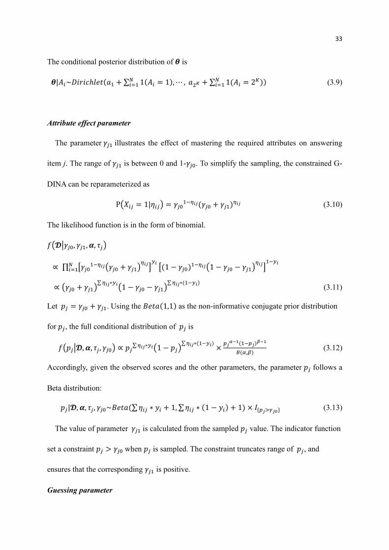
Attribute effect parameter

The parameter 𝛾𝑗1 illustrates the effect of mastering the required attributes on answering

item j. The range of 𝛾𝑗1 is between 0 and 1-𝛾𝑗0. To simplify the sampling, the constrained G-

DINA can be reparameterized as

P(𝑋𝑖𝑗 = 1|𝜂𝑖𝑗) = 𝛾𝑗01−𝜂𝑖𝑗(𝛾𝑗0 + 𝛾𝑗1)

𝜂𝑖𝑗 (3.10)

The likelihood function is in the form of binomial.

𝑓(𝓓|𝛾𝑗0, 𝛾𝑗1, 𝜶, 𝜏𝑗 )

∝ ∏ [𝛾𝑗01−𝜂𝑖𝑗(𝛾𝑗0 + 𝛾𝑗1)

𝜂𝑖𝑗]𝑦𝑖𝑁

𝑖=1 [(1 − 𝛾𝑗0)1−𝜂𝑖𝑗(1 − 𝛾𝑗0 − 𝛾𝑗1)

𝜂𝑖𝑗]1−𝑦𝑖

∝ (𝛾𝑗0 + 𝛾𝑗1)∑𝜂𝑖𝑗∗𝑦𝑖

(1 − 𝛾𝑗0 − 𝛾𝑗1)∑𝜂𝑖𝑗∗(1−𝑦𝑖)

(3.11)

Let 𝑝𝑗 = 𝛾𝑗0 + 𝛾𝑗1. Using the 𝐵𝑒𝑡𝑎(1,1) as the non-informative conjugate prior distribution

for 𝑝𝑗, the full conditional distribution of 𝑝𝑗 is

𝑓(𝑝𝑗|𝓓, 𝜶, 𝜏𝑗 , 𝛾𝑗0) ∝ 𝑝𝑗

∑𝜂𝑖𝑗∗𝑦𝑖(1 − 𝑝𝑗)∑𝜂𝑖𝑗∗(1−𝑦𝑖)

×𝑝𝑗𝛼−1(1−𝑝𝑗)

𝛽−1

𝐵(𝛼,𝛽) (3.12)

Accordingly, given the observed scores and the other parameters, the parameter 𝑝𝑗 follows a

Beta distribution:

𝑝𝑗|𝓓, 𝜶, 𝜏𝑗 , 𝛾𝑗0~𝐵𝑒𝑡𝑎(∑𝜂𝑖𝑗 ∗ 𝑦𝑖 + 1, ∑𝜂𝑖𝑗 ∗ (1 − 𝑦𝑖) + 1) × 𝐼{𝑝𝑗>𝛾𝑗0} (3.13)

The value of parameter 𝛾𝑗1 is calculated from the sampled 𝑝𝑗 value. The indicator function

set a constraint 𝑝𝑗 > 𝛾𝑗0 when 𝑝𝑗 is sampled. The constraint truncates range of 𝑝𝑗, and

ensures that the corresponding 𝛾𝑗1 is positive.

Guessing parameter

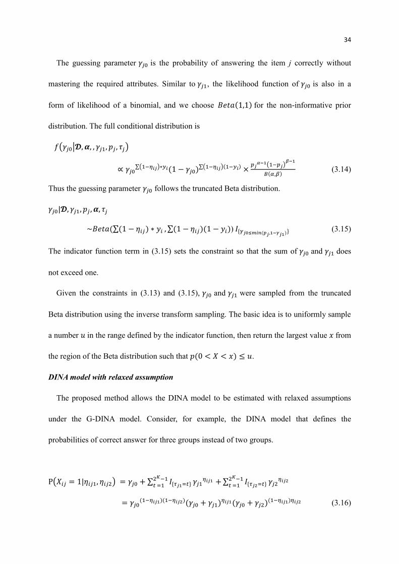
34

The guessing parameter 𝛾𝑗0 is the probability of answering the item j correctly without

mastering the required attributes. Similar to 𝛾𝑗1, the likelihood function of 𝛾𝑗0 is also in a

form of likelihood of a binomial, and we choose 𝐵𝑒𝑡𝑎(1,1) for the non-informative prior

distribution. The full conditional distribution is

𝑓(𝛾𝑗0|𝓓, 𝜶, , 𝛾𝑗1, 𝑝𝑗 , 𝜏𝑗 )

∝ 𝛾𝑗0∑(1−𝜂𝑖𝑗)∗𝑦𝑖(1 − 𝛾𝑗0)

∑(1−𝜂𝑖𝑗)(1−𝑦𝑖) ×𝑝𝑗𝛼−1(1−𝑝𝑗)

𝛽−1

𝐵(𝛼,𝛽) (3.14)

Thus the guessing parameter 𝛾𝑗0 follows the truncated Beta distribution.

𝛾𝑗0|𝓓, 𝛾𝑗1, 𝑝𝑗 , 𝜶, 𝜏𝑗

~𝐵𝑒𝑡𝑎(∑(1 − 𝜂𝑖𝑗) ∗ 𝑦𝑖 , ∑(1 − 𝜂𝑖𝑗)(1 − 𝑦𝑖)) 𝐼{𝛾𝑗0≤𝑚𝑖𝑛 (𝑝𝑗,1−𝛾𝑗1)} (3.15)

The indicator function term in (3.15) sets the constraint so that the sum of 𝛾𝑗0 and 𝛾𝑗1 does

not exceed one.

Given the constraints in (3.13) and (3.15), 𝛾𝑗0 and 𝛾𝑗1 were sampled from the truncated

Beta distribution using the inverse transform sampling. The basic idea is to uniformly sample

a number 𝑢 in the range defined by the indicator function, then return the largest value 𝑥 from

the region of the Beta distribution such that 𝑝(0 < 𝑋 < 𝑥) ≤ 𝑢.

DINA model with relaxed assumption

The proposed method allows the DINA model to be estimated with relaxed assumptions

under the G-DINA model. Consider, for example, the DINA model that defines the

probabilities of correct answer for three groups instead of two groups.

P(𝑋𝑖𝑗 = 1|𝜂𝑖𝑗1, 𝜂𝑖𝑗2) = 𝛾𝑗0 + ∑ 𝐼{𝜏𝑗1=𝑡}2𝐾−1𝑡 =1

𝛾𝑗1𝜂𝑖𝑗1 +∑ 𝐼{𝜏𝑗2=𝑡}

2𝐾−1𝑡 =1

𝛾𝑗2𝜂𝑖𝑗2

= 𝛾𝑗0(1−𝜂𝑖𝑗1)(1−𝜂𝑖𝑗2)(𝛾𝑗0 + 𝛾𝑗1)

𝜂𝑖𝑗1(𝛾𝑗0 + 𝛾𝑗2)(1−𝜂𝑖𝑗1)𝜂𝑖𝑗2 (3.16)

35

Compared with the DINA model, the relaxed version (3.16) includes the partial credit

indicator 𝜂𝑖𝑗2, and the corresponding effect 𝛾𝑗2. Specifically, if the individual i masters the

required attribute in 𝜂𝑖𝑗1 of item j, the probability of correct answer is (𝛾𝑗0 + 𝛾𝑗1); however, if

this individual does not master attributes defined by 𝜂𝑖𝑗1 but masters the required attributes in

𝜂𝑖𝑗2, the probability of answering the item correctly is (𝛾𝑗0 + 𝛾𝑗2) instead of 𝛾𝑗0 . Note

that 𝛾𝑗1 > 𝛾𝑗2 . In other words, 𝜂𝑖𝑗2 can be interpreted that given the individual does not

master all the required attributes indicated by 𝜂𝑖𝑗1，whether the individual masters some

attributes that make answer better than simply guessing. These attributes give the individual

some partial credit. If so, the probability is (𝛾𝑗0 + 𝛾𝑗2), which is lower than (𝛾𝑗0 + 𝛾𝑗1), but it

is higher than 𝛾𝑗0.

Gibbs sampling is still applicable to this relaxed version of DINA model. Given other

parameters, the term 𝛾𝑗0 + 𝛾𝑗2 follows a Beta distribution. When the item class is sampled,

we sample two values, one for the estimation of item class, and the other for the partial credit

class. By adding more partial credit indicators, there will be more attribute-combinations

receive the corresponding partial credits, and so the DINA model assumption is further

relaxed. Adding more parameters may result in better data fit, but the partial credit

parameters also bring more assumptions into the model.

3.3 Re-labeling and Finalizing Q-matrix

The label switching problem arises when taking Bayesian approach to the parameter

estimation and clustering using mixture models (Stephens, 2000). The term label switching

36

was used by Redner and Walker (1984) to describe the invariance of the likelihood under

relabeling of the mixture components. In the present study, the likelihood is invariant under

the permutation of the K attributes. The value of 𝜂𝑖𝑗𝜏𝑗∗ remains the same if the columns of Q-

matrix are in different order. Without prior information that distinguishes these attributes, the

posterior distributions are similarly symmetric, and so the label switching is possible in the

sampling result. If the label switching happens, summary statistics of the marginal

distributions will not give accurate estimates (Stephens, 1997).

In the present study, there is no underlying order of these attribute, which makes it hard to

formulate the prior to avoid the label switching. This problem is ignored during the sampling,

and the output is then post-processed by re-labeling the attributes to keep the labels consistent

across all the sampling matrices. The basic elements of the re-labeling are the following:

1. Calculate the average Q-matrix and the average 𝜶 matrix with all the sampling

outputs after burn-in.

2. Pick the permutation for the sampling outputs of each iteration which gives the

smallest Euclidean distance between the sampling outputs.

3. Apply the selected permutation on the corresponding outputs, and update the average

Q-matrix and the average 𝜶 matrix.

4. Iterate Step 2 and 3 until a convergence attained.

The purpose of the relabeling is to make the column order of sampling from each iteration

matches the column order of one another.Suppose there is no label switching in the sampling

results, then it is simple to finalize the Q-matrix by taking average of the sampling results.

Now consider that the column order of part of the samplings are different from the majority,

37

then permute the columns of these samplings will make the new average matrix closer to the

average matrix that is free from label switching.

3.4 Study designs

The present paper involves one simulation study and one empirical study. The simulation

studies were designed to examine the model performance under different scenarios. The

model performance is basically evaluated with the accuracy of the Q-matrix estimation

compared to the true Q-matrix. The recovery of the guessing and the slipping parameters

were also considered. The design conditions vary in sample size and the correlation of the

attributes.

The possession of the attributes could be correlated or uncorrelated according to different

situations. The artificial data in the simulation studies of the present paper were created

assuming that the attributes were correlated. Emrich and Piedmonte (1991) proposed a

method to generate the multivariate correlated binary covariates according to the

predetermined correlation matrix. Given the marginal expectation 𝒑 = (𝑝𝑖, ⋯ , 𝑝𝐾) and the

correlation matrix 𝜟 = (𝛿𝑖𝑗)𝐾×𝐾 , a K-dimensional multivariate normal vector 𝒁 =

(𝑍1, ⋯ , 𝑍𝐾) can be created with the mean 𝝁 and the correlation matrix 𝑹 = (𝜌𝑖𝑗)𝐾×𝐾 .

Let 𝝁 = 𝜱−𝟏(𝒑), then

𝑝𝑖 = 𝑃(𝑋𝑖 = 1) = 𝑃(𝑍𝑖 > 0) = 𝑃((𝑍𝑖 − 𝜇𝑖) < 𝜇𝑖) = 𝛷(𝜇𝑖) (3.17)

where 𝛷(∙) is the standard normal distribution, and

𝑝𝑖𝑗 = 𝑃(𝑋𝑖 = 1, 𝑋𝑗 = 1) = 𝑃(𝑍𝑖 − 𝜇𝑖 ≤ 𝜇𝑖, 𝑍𝑗 − 𝜇𝑗 ≤ 𝜇𝑗) = 𝛷(𝜇𝑖, 𝜇𝑗; 𝜌𝑖𝑗) (3.18)

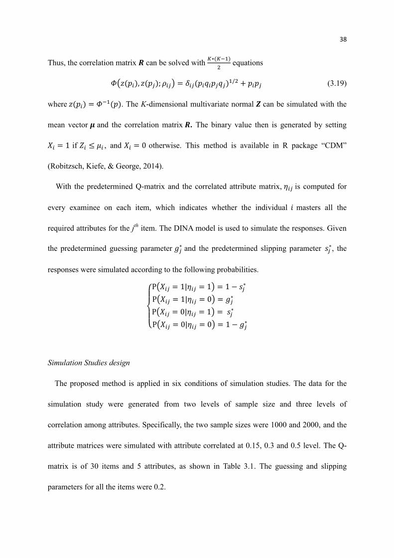
38

Thus, the correlation matrix 𝑹 can be solved with 𝐾∗(𝐾−1)

2 equations

𝛷(𝑧(𝑝𝑖), 𝑧(𝑝𝑗); 𝜌𝑖𝑗) = 𝛿𝑖𝑗(𝑝𝑖𝑞𝑖𝑝𝑗𝑞𝑗)1/2 + 𝑝𝑖𝑝𝑗 (3.19)

where 𝑧(𝑝𝑖) = 𝛷−1(𝑝). The K-dimensional multivariate normal 𝒁 can be simulated with the

mean vector 𝝁 and the correlation matrix 𝑹. The binary value then is generated by setting

𝑋𝑖 = 1 if 𝑍𝑖 ≤ 𝜇𝑖 , and 𝑋𝑖 = 0 otherwise. This method is available in R package “CDM”

(Robitzsch, Kiefe, & George, 2014).

With the predetermined Q-matrix and the correlated attribute matrix, 𝜂𝑖𝑗 is computed for

every examinee on each item, which indicates whether the individual 𝑖 masters all the

required attributes for the jth

item. The DINA model is used to simulate the responses. Given

the predetermined guessing parameter 𝑔𝑗∗ and the predetermined slipping parameter 𝑠𝑗

∗, the

responses were simulated according to the following probabilities.

{

P(𝑋𝑖𝑗 = 1|𝜂𝑖𝑗 = 1) = 1 − 𝑠𝑗

∗

P(𝑋𝑖𝑗 = 1|𝜂𝑖𝑗 = 0) = 𝑔𝑗∗

P(𝑋𝑖𝑗 = 0|𝜂𝑖𝑗 = 1) = 𝑠𝑗∗

P(𝑋𝑖𝑗 = 0|𝜂𝑖𝑗 = 0) = 1 − 𝑔𝑗∗

Simulation Studies design

The proposed method is applied in six conditions of simulation studies. The data for the

simulation study were generated from two levels of sample size and three levels of

correlation among attributes. Specifically, the two sample sizes were 1000 and 2000, and the

attribute matrices were simulated with attribute correlated at 0.15, 0.3 and 0.5 level. The Q-

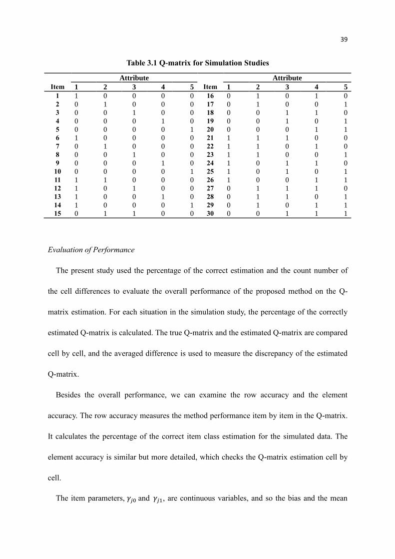
matrix is of 30 items and 5 attributes, as shown in Table 3.1. The guessing and slipping

parameters for all the items were 0.2.

39

Table 3.1 Q-matrix for Simulation Studies

Attribute Attribute

Item 1 2 3 4 5 Item 1 2 3 4 5

1 1 0 0 0 0 16 0 1 0 1 0

2 0 1 0 0 0 17 0 1 0 0 1

3 0 0 1 0 0 18 0 0 1 1 0

4 0 0 0 1 0 19 0 0 1 0 1

5 0 0 0 0 1 20 0 0 0 1 1

6 1 0 0 0 0 21 1 1 1 0 0

7 0 1 0 0 0 22 1 1 0 1 0

8 0 0 1 0 0 23 1 1 0 0 1

9 0 0 0 1 0 24 1 0 1 1 0

10 0 0 0 0 1 25 1 0 1 0 1

11 1 1 0 0 0 26 1 0 0 1 1

12 1 0 1 0 0 27 0 1 1 1 0

13 1 0 0 1 0 28 0 1 1 0 1

14 1 0 0 0 1 29 0 1 0 1 1

15 0 1 1 0 0 30 0 0 1 1 1

Evaluation of Performance

The present study used the percentage of the correct estimation and the count number of

the cell differences to evaluate the overall performance of the proposed method on the Q-

matrix estimation. For each situation in the simulation study, the percentage of the correctly

estimated Q-matrix is calculated. The true Q-matrix and the estimated Q-matrix are compared

cell by cell, and the averaged difference is used to measure the discrepancy of the estimated

Q-matrix.

Besides the overall performance, we can examine the row accuracy and the element

accuracy. The row accuracy measures the method performance item by item in the Q-matrix.

It calculates the percentage of the correct item class estimation for the simulated data. The

element accuracy is similar but more detailed, which checks the Q-matrix estimation cell by

cell.

The item parameters, 𝛾𝑗0 and 𝛾𝑗1, are continuous variables, and so the bias and the mean

40

squared error are used to evaluate the proposed method performance. The bias is the

difference between the predetermined parameter values and the average of the estimations.

Empirical Study

The proposed method was also applied to real data for the Q-matrix estimation. The

fraction subtraction dataset is a well-known data in the Q-matrix research and is widely

analyzed. The Tatsuoka’s fraction subtraction data set is comprised of 536 rows and 20

columns, representing the responses of 536 middle school students to each of the 20 fraction

subtraction test items. Each row in the data set corresponds to the responses of a particular

student. Value “1” denotes that a correct response was recorded, and “0” denotes an incorrect

response. All test items are based on 8 attributes. The Q-matrix can be found in DeCarlo

(2011), and it was also used by de la Torre and Douglas (2004).

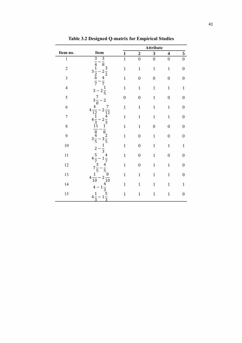
Another version of the fraction subtraction data set consists of 15 items and 536 students.

The Q-matrix (Table 3.2) was defined in the de la Torre (2009). There are five required

attributes, including: (1) subtract numerators, (2) reduce answers to simplest form, (3)

separate a whole number from a fraction, (4) borrow from a whole number part, and (5)

convert a whole number to a fraction. The present paper takes dataset of the 15 items version

for the empirical study.

41

Table 3.2 Designed Q-matrix for Empirical Studies

Item no.

Item

Attribute

1 2 3 4 5

1 3

4−3

8

1 0 0 0 0

2 31

2− 2

3

2

1 1 1 1 0

3 6

7−4

7

1 0 0 0 0

4 3 − 2

1

5

1 1 1 1 1

5 37

8− 2

0 0 1 0 0

6 44

12− 2

7

12

1 1 1 1 0

7 41

3− 2

4

3

1 1 1 1 0

8 11

8−1

8

1 1 0 0 0

9 34

5− 3

2

5

1 0 1 0 0

10 2 −

1

3

1 0 1 1 1

11 45

7− 1

4

7

1 0 1 0 0

12 73

5−4

5

1 0 1 1 0

13 41

10− 2

8

10

1 1 1 1 0

14 4 − 1

4

3

1 1 1 1 1

15 41

3− 1

5

3

1 1 1 1 0

42

Chapter 4

Results

In this chapter, we present the results of the simulation study and the empirical study. The

data for the simulation study were generated from two levels of sample size and three levels

of correlation among attributes. Specifically, the two sample sizes were 1000 and 2000, and

the attribute matrices were simulated with attribute correlated at 0.15, 0.3 and 0.5 level. Thus

six conditions were considered. Results for one simulated data set were presented in detail, in

order to show how the proposed method estimated the Q-matrix, examinees’ attributes and

the item parameters. Then the results of the simulation study were summarized into the count

number of the correctly estimated Q-matrix under each condition. The simulation results

were further evaluated with the logistic regression models to check the effect of conditions. In

the empirical study, the fraction subtraction data set that consisted of 15 items and 536

students was used. The Q-matrix of fraction subtraction data was separately estimated with

the proposed methods for 4 times.

4.1 Simulation Study Results

The present simulation study considers two levels for sample size. Regarding the 1000

sample size condition, the length of the sampling was 15000 and the burn-in was 10000. A

number of estimation trails were used to determine the length of sampling and the burn-in

43

value. The diagnostic plots of moving average for Q-matrix were inspected, which were

shown as Figure 4.1. For most of the times the sampling distribution would converge to the

limit distribution with 5000 to 10000 samples. For the 2000 sample size conditions, the

15000 sampling length was not enough, and the chains with 50000 sampled values were used,

because we observed that the necessary iteration for convergence varies a lot for 2000 sample

size conditions.

4.1.1 Results for one simulated data set

In order to illustrate how the proposed method works, the estimated outputs for one of the

simulated datasets were presented in details. The chosen dataset was under the condition that

the attribute correlations were all at 0.5 and sample size was 1000. The estimations for the Q-

matrix, the attribute profiles and the item parameters for the chosen dataset were shown

within this section.

The Q-matrix

The average of the sampled Q-matrix after burn-ins was presented in Table 4.1. The

number in each cell is the fraction of sampling 1 out of all the samples after burn-in. For

example, if the value in the item one and attribute one cell is 0.7, it means that among all the

5000 samples after burn-in 70% samples are 1 and 30% of them are 0. If the decimals in the

table were dichotomized to 0 and 1 with the cutoff at 0.5, the table would be identical to the

predetermined Q-matrix in Table 3.1.

The distance between the predetermined Q-matrix and the moving average of the estimated

Q-matrix decreased as the sampling went on, as shown in Figure 4.1. The bandwidth of the

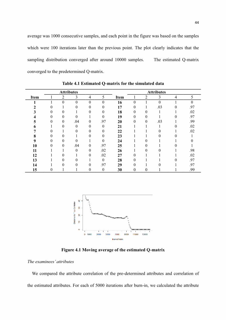
44

average was 1000 consecutive samples, and each point in the figure was based on the samples

which were 100 iterations later than the previous point. The plot clearly indicates that the

sampling distribution converged after around 10000 samples. The estimated Q-matrix

converged to the predetermined Q-matrix.

Table 4.1 Estimated Q-matrix for the simulated data

Attributes Attributes

Item 1 2 3 4 5 Item 1 2 3 4 5

1 1 0 0 0 0 16 0 1 0 1 0

2 0 1 0 0 0 17 0 1 .03 0 .97

3 0 0 1 0 0 18 0 0 1 1 .02

4 0 0 0 1 0 19 0 0 1 0 .97

5 0 0 .04 0 .97 20 0 0 .03 1 .99

6 1 0 0 0 0 21 1 1 1 0 .02

7 0 1 0 0 0 22 1 1 0 1 .02

8 0 0 1 0 0 23 1 1 0 0 1

9 0 0 0 1 0 24 1 0 1 1 0

10 0 0 .04 0 .97 25 1 0 1 0 1

11 1 1 0 0 .02 26 1 0 0 1 .98

12 1 0 1 0 .02 27 0 1 1 1 .02

13 1 0 0 1 0 28 0 1 1 0 .97

14 1 0 0 0 .97 29 0 1 0 1 .97

15 0 1 1 0 0 30 0 0 1 1 .99

Figure 4.1 Moving average of the estimated Q-matrix

The examinees’ attributes

We compared the attribute correlation of the pre-determined attributes and correlation of

the estimated attributes. For each of 5000 iterations after burn-in, we calculated the attribute

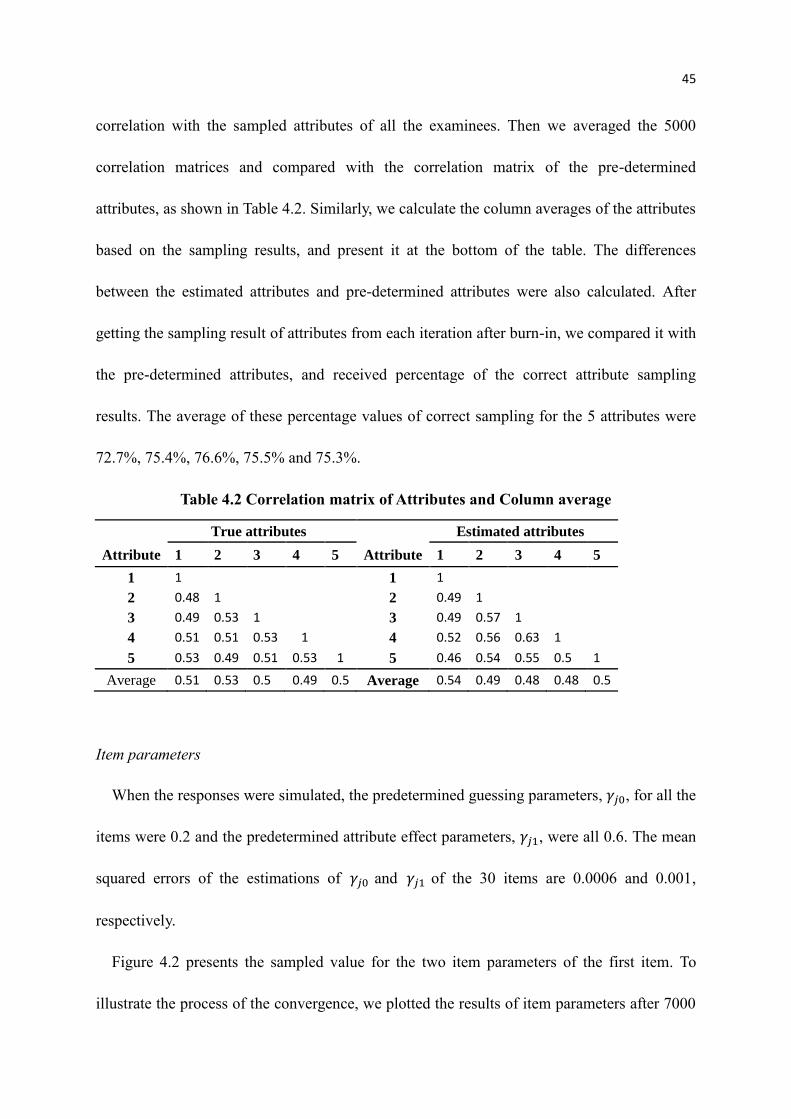
45

correlation with the sampled attributes of all the examinees. Then we averaged the 5000

correlation matrices and compared with the correlation matrix of the pre-determined

attributes, as shown in Table 4.2. Similarly, we calculate the column averages of the attributes

based on the sampling results, and present it at the bottom of the table. The differences

between the estimated attributes and pre-determined attributes were also calculated. After

getting the sampling result of attributes from each iteration after burn-in, we compared it with

the pre-determined attributes, and received percentage of the correct attribute sampling

results. The average of these percentage values of correct sampling for the 5 attributes were

72.7%, 75.4%, 76.6%, 75.5% and 75.3%.

Table 4.2 Correlation matrix of Attributes and Column average

True attributes Estimated attributes

Attribute 1 2 3 4 5 Attribute 1 2 3 4 5

1 1

1 1

2 0.48 1

2 0.49 1

3 0.49 0.53 1

3 0.49 0.57 1

4 0.51 0.51 0.53 1

4 0.52 0.56 0.63 1

5 0.53 0.49 0.51 0.53 1 5 0.46 0.54 0.55 0.5 1

Average 0.51 0.53 0.5 0.49 0.5 Average 0.54 0.49 0.48 0.48 0.5

Item parameters

When the responses were simulated, the predetermined guessing parameters, 𝛾𝑗0, for all the

items were 0.2 and the predetermined attribute effect parameters, 𝛾𝑗1, were all 0.6. The mean

squared errors of the estimations of 𝛾𝑗0 and 𝛾𝑗1 of the 30 items are 0.0006 and 0.001,

respectively.

Figure 4.2 presents the sampled value for the two item parameters of the first item. To

illustrate the process of the convergence, we plotted the results of item parameters after 7000

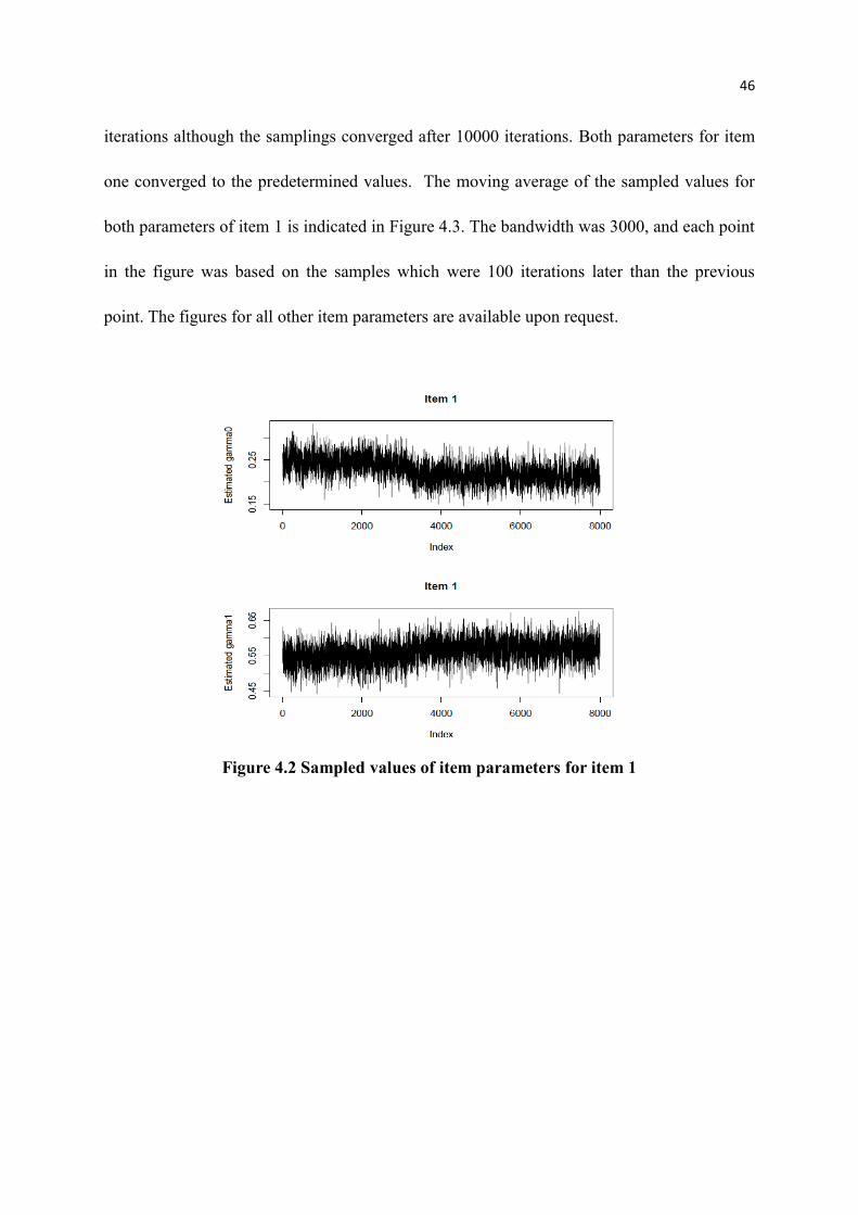
46

iterations although the samplings converged after 10000 iterations. Both parameters for item

one converged to the predetermined values. The moving average of the sampled values for

both parameters of item 1 is indicated in Figure 4.3. The bandwidth was 3000, and each point

in the figure was based on the samples which were 100 iterations later than the previous

point. The figures for all other item parameters are available upon request.

Figure 4.2 Sampled values of item parameters for item 1

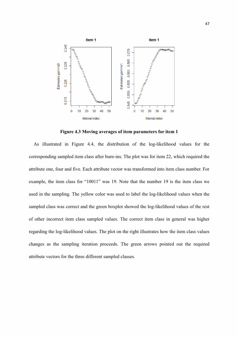
47

Figure 4.3 Moving averages of item parameters for item 1

As illustrated in Figure 4.4, the distribution of the log-likelihood values for the

corresponding sampled item class after burn-ins. The plot was for item 22, which required the

attribute one, four and five. Each attribute vector was transformed into item class number. For

example, the item class for “10011” was 19. Note that the number 19 is the item class we

used in the sampling. The yellow color was used to label the log-likelihood values when the

sampled class was correct and the green boxplot showed the log-likelihood values of the rest

of other incorrect item class sampled values. The correct item class in general was higher

regarding the log-likelihood values. The plot on the right illustrates how the item class values

changes as the sampling iteration proceeds. The green arrows pointed out the required

attribute vectors for the three different sampled classes.

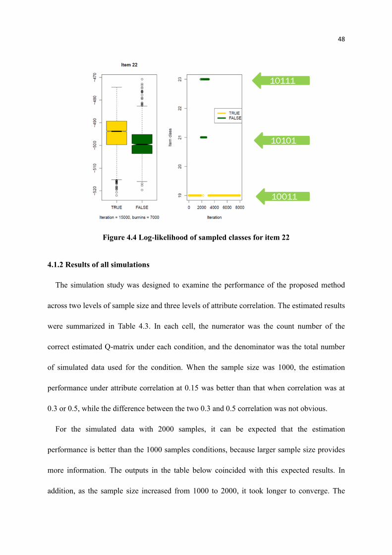
48

Figure 4.4 Log-likelihood of sampled classes for item 22

4.1.2 Results of all simulations

The simulation study was designed to examine the performance of the proposed method

across two levels of sample size and three levels of attribute correlation. The estimated results

were summarized in Table 4.3. In each cell, the numerator was the count number of the

correct estimated Q-matrix under each condition, and the denominator was the total number

of simulated data used for the condition. When the sample size was 1000, the estimation

performance under attribute correlation at 0.15 was better than that when correlation was at

0.3 or 0.5, while the difference between the two 0.3 and 0.5 correlation was not obvious.

For the simulated data with 2000 samples, it can be expected that the estimation

performance is better than the 1000 samples conditions, because larger sample size provides

more information. The outputs in the table below coincided with this expected results. In

addition, as the sample size increased from 1000 to 2000, it took longer to converge. The

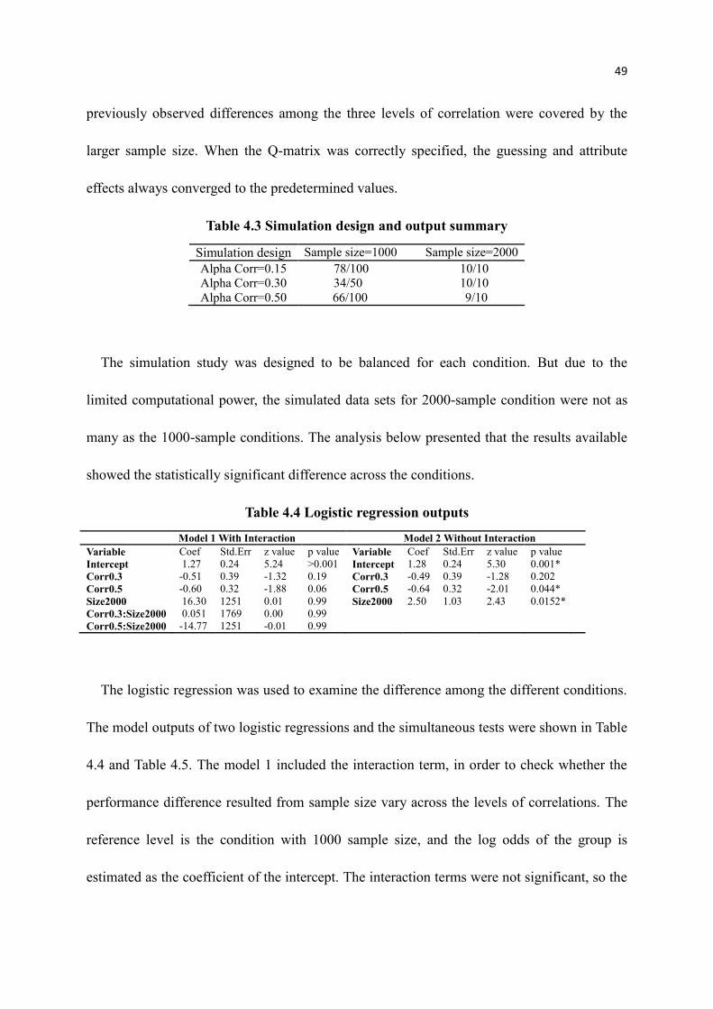
49

previously observed differences among the three levels of correlation were covered by the

larger sample size. When the Q-matrix was correctly specified, the guessing and attribute

effects always converged to the predetermined values.

Table 4.3 Simulation design and output summary

Simulation design Sample size=1000 Sample size=2000

Alpha Corr=0.15 78/100 10/10

Alpha Corr=0.30 34/50 10/10

Alpha Corr=0.50 66/100 9/10

The simulation study was designed to be balanced for each condition. But due to the

limited computational power, the simulated data sets for 2000-sample condition were not as

many as the 1000-sample conditions. The analysis below presented that the results available

showed the statistically significant difference across the conditions.

Table 4.4 Logistic regression outputs

Model 1 With Interaction Model 2 Without Interaction

Variable Coef Std.Err z value p value Variable Coef Std.Err z value p value

Intercept 1.27 0.24 5.24 >0.001 Intercept 1.28 0.24 5.30 0.001*

Corr0.3 -0.51 0.39 -1.32 0.19 Corr0.3 -0.49 0.39 -1.28 0.202

Corr0.5 -0.60 0.32 -1.88 0.06 Corr0.5 -0.64 0.32 -2.01 0.044*

Size2000 16.30 1251 0.01 0.99 Size2000 2.50 1.03 2.43 0.0152*

Corr0.3:Size2000 0.051 1769 0.00 0.99

Corr0.5:Size2000 -14.77 1251 -0.01 0.99

The logistic regression was used to examine the difference among the different conditions.

The model outputs of two logistic regressions and the simultaneous tests were shown in Table

4.4 and Table 4.5. The model 1 included the interaction term, in order to check whether the

performance difference resulted from sample size vary across the levels of correlations. The

reference level is the condition with 1000 sample size, and the log odds of the group is

estimated as the coefficient of the intercept. The interaction terms were not significant, so the

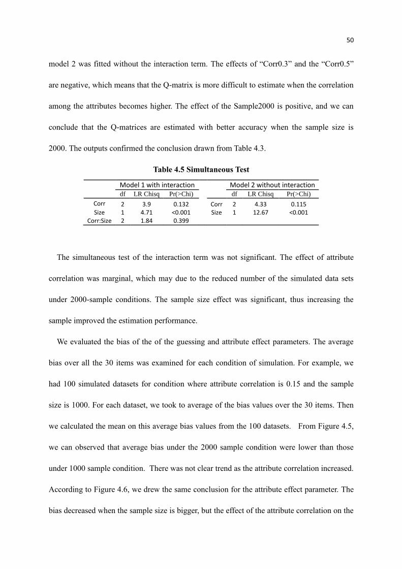
50

model 2 was fitted without the interaction term. The effects of “Corr0.3” and the “Corr0.5”

are negative, which means that the Q-matrix is more difficult to estimate when the correlation

among the attributes becomes higher. The effect of the Sample2000 is positive, and we can

conclude that the Q-matrices are estimated with better accuracy when the sample size is

2000. The outputs confirmed the conclusion drawn from Table 4.3.

Table 4.5 Simultaneous Test

Model 1 with interaction

Model 2 without interaction

df LR Chisq Pr(>Chi)

df LR Chisq Pr(>Chi)

Corr 2 3.9 0.132

Corr 2 4.33 0.115 Size 1 4.71 <0.001

Size 1 12.67 <0.001

Corr:Size 2 1.84 0.399

The simultaneous test of the interaction term was not significant. The effect of attribute

correlation was marginal, which may due to the reduced number of the simulated data sets

under 2000-sample conditions. The sample size effect was significant, thus increasing the

sample improved the estimation performance.

We evaluated the bias of the of the guessing and attribute effect parameters. The average

bias over all the 30 items was examined for each condition of simulation. For example, we

had 100 simulated datasets for condition where attribute correlation is 0.15 and the sample

size is 1000. For each dataset, we took to average of the bias values over the 30 items. Then

we calculated the mean on this average bias values from the 100 datasets. From Figure 4.5,

we can observed that average bias under the 2000 sample condition were lower than those

under 1000 sample condition. There was not clear trend as the attribute correlation increased.

According to Figure 4.6, we drew the same conclusion for the attribute effect parameter. The

bias decreased when the sample size is bigger, but the effect of the attribute correlation on the

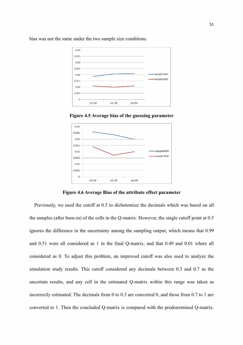
51

bias was not the same under the two sample size conditions.

Figure 4.5 Average bias of the guessing parameter

Figure 4.6 Average Bias of the attribute effect parameter

Previously, we used the cutoff at 0.5 to dichotomize the decimals which was based on all

the samples (after burn-in) of the cells in the Q-matrix. However, the single cutoff point at 0.5

ignores the difference in the uncertainty among the sampling output, which means that 0.99

and 0.51 were all considered as 1 in the final Q-matrix, and that 0.49 and 0.01 where all

considered as 0. To adjust this problem, an improved cutoff was also used to analyze the

simulation study results. This cutoff considered any decimals between 0.3 and 0.7 as the

uncertain results, and any cell in the estimated Q-matrix within this range was taken as

incorrectly estimated. The decimals from 0 to 0.3 are converted 0, and those from 0.7 to 1 are

converted to 1. Then the concluded Q-matrix is compared with the predetermined Q-matrix.

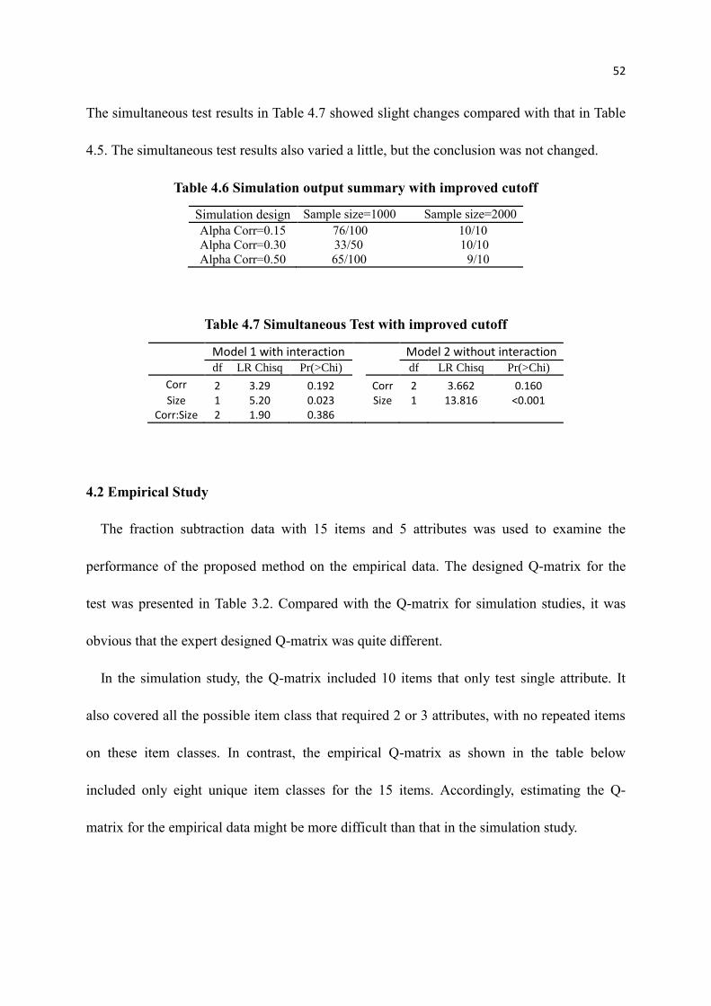
52

The simultaneous test results in Table 4.7 showed slight changes compared with that in Table

4.5. The simultaneous test results also varied a little, but the conclusion was not changed.

Table 4.6 Simulation output summary with improved cutoff

Simulation design Sample size=1000 Sample size=2000

Alpha Corr=0.15 76/100 10/10

Alpha Corr=0.30 33/50 10/10

Alpha Corr=0.50 65/100 9/10

Table 4.7 Simultaneous Test with improved cutoff

Model 1 with interaction

Model 2 without interaction

df LR Chisq Pr(>Chi)

df LR Chisq Pr(>Chi)

Corr 2 3.29 0.192

Corr 2 3.662 0.160 Size 1 5.20 0.023

Size 1 13.816 <0.001

Corr:Size 2 1.90 0.386

4.2 Empirical Study

The fraction subtraction data with 15 items and 5 attributes was used to examine the

performance of the proposed method on the empirical data. The designed Q-matrix for the

test was presented in Table 3.2. Compared with the Q-matrix for simulation studies, it was

obvious that the expert designed Q-matrix was quite different.

In the simulation study, the Q-matrix included 10 items that only test single attribute. It

also covered all the possible item class that required 2 or 3 attributes, with no repeated items

on these item classes. In contrast, the empirical Q-matrix as shown in the table below

included only eight unique item classes for the 15 items. Accordingly, estimating the Q-

matrix for the empirical data might be more difficult than that in the simulation study.

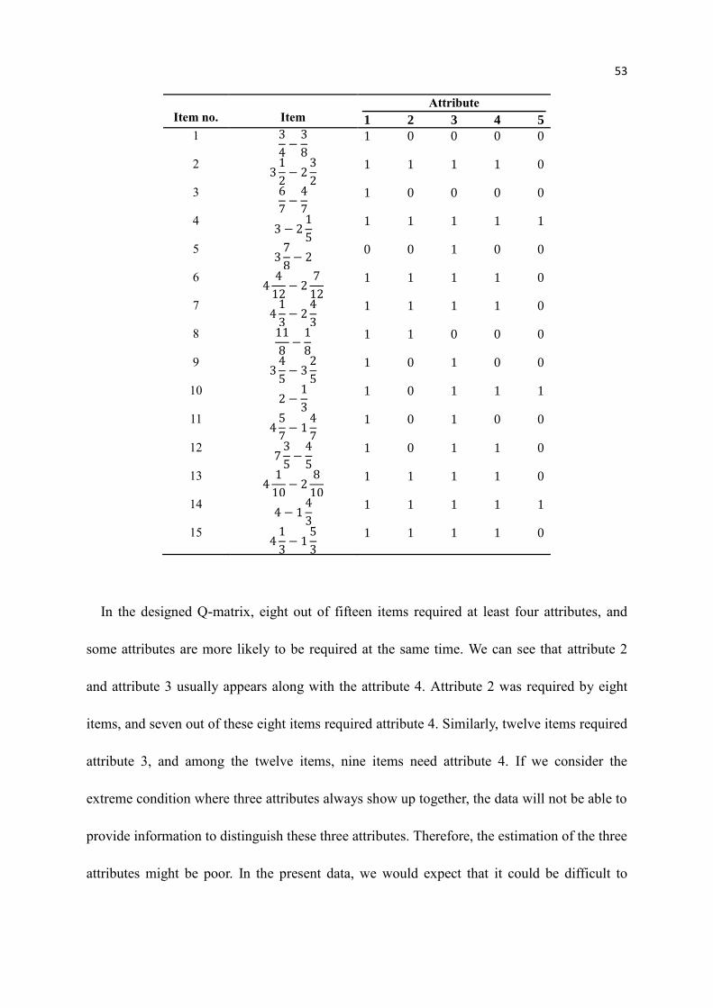
53

Item no.

Item

Attribute

1 2 3 4 5

1 3

4−3

8

1 0 0 0 0

2 31

2− 2

3

2

1 1 1 1 0

3 6

7−4

7

1 0 0 0 0

4 3 − 2

1

5

1 1 1 1 1

5 37

8− 2

0 0 1 0 0

6 44

12− 2

7

12

1 1 1 1 0

7 41

3− 2

4

3

1 1 1 1 0

8 11

8−1

8

1 1 0 0 0

9 34

5− 3

2

5

1 0 1 0 0

10 2 −

1

3

1 0 1 1 1

11 45

7− 1

4

7

1 0 1 0 0

12 73

5−4

5

1 0 1 1 0

13 41

10− 2

8

10

1 1 1 1 0

14 4 − 1

4

3

1 1 1 1 1

15 41

3− 1

5

3

1 1 1 1 0

In the designed Q-matrix, eight out of fifteen items required at least four attributes, and

some attributes are more likely to be required at the same time. We can see that attribute 2

and attribute 3 usually appears along with the attribute 4. Attribute 2 was required by eight

items, and seven out of these eight items required attribute 4. Similarly, twelve items required

attribute 3, and among the twelve items, nine items need attribute 4. If we consider the

extreme condition where three attributes always show up together, the data will not be able to

provide information to distinguish these three attributes. Therefore, the estimation of the three

attributes might be poor. In the present data, we would expect that it could be difficult to

54

estimate these three attributes in the Q-matrix.

Four separate sampling processes were carried out on the empirical data. Each chain

contained 70000 sampled values, and the estimation was based on the last 10000 samples.

For attribute 2, 4 and 5, the empirical test did not contain the items that only ask for a single

attribute, and so it is difficult to decide how to permute the order of attributes in the sampled

Q-matrix. To find the appropriate permutation for the Q-matrix, all the possible permutations

were applied to the sampled Q-matrix. Then the estimated Q-matrices with permutated

columns were compared with the designed Q-matrix. The permutations that gave the

estimated Q-matrices closest to the designed Q-matrix were considered as the appropriate

permutations.

For example, in the results of the Estimation 1 as shown in Table 4.8, the lowest count of

the mis-specified cell in the estimated Q-matrix was twenty after all 120 permutations were

checked. Four out of the 120 permutations gave the estimated Q-matrix of this level of

correctness. All of the four permutations picked the column 5 for attribute1 and column 3 for

attribute 5. However, the estimated Q-matrix could not determine the attribute 2, 3 and 4

because the different order of these three columns led to the Q-matrices at the same level of

correctness.

As the discussion above, the attribute 2, 3 and 4 were usually required together, and this

could be one of the reasons for the difficulty in the estimation. The sampling process was

plotted in Figure 4.7. The plot indicated the count of different cells between estimated Q-

matrix and the designed Q-matrix. Each point is the average of 1000 consecutive samples of

Q-matrix, and from point to point, the average samples moved 100 forward. It can be

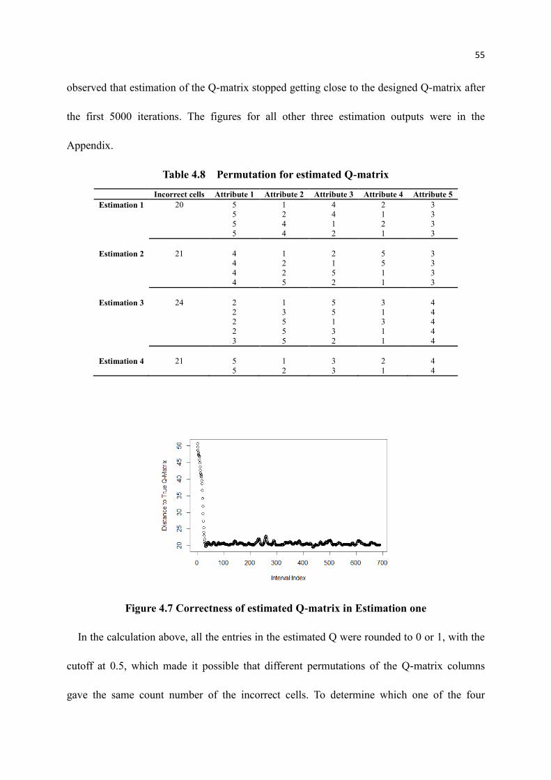
55

observed that estimation of the Q-matrix stopped getting close to the designed Q-matrix after

the first 5000 iterations. The figures for all other three estimation outputs were in the

Appendix.

Table 4.8 Permutation for estimated Q-matrix

Incorrect cells Attribute 1 Attribute 2 Attribute 3 Attribute 4 Attribute 5

Estimation 1 20 5 1 4 2 3

5 2 4 1 3

5 4 1 2 3

5 4 2 1 3

Estimation 2 21 4 1 2 5 3

4 2 1 5 3

4 2 5 1 3

4 5 2 1 3

Estimation 3 24 2 1 5 3 4

2 3 5 1 4

2 5 1 3 4

2 5 3 1 4

3 5 2 1 4

Estimation 4 21 5 1 3 2 4

5 2 3 1 4

Figure 4.7 Correctness of estimated Q-matrix in Estimation one

In the calculation above, all the entries in the estimated Q were rounded to 0 or 1, with the

cutoff at 0.5, which made it possible that different permutations of the Q-matrix columns

gave the same count number of the incorrect cells. To determine which one of the four

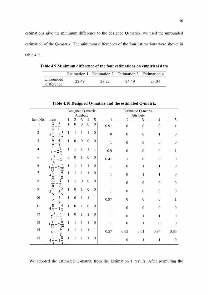
56

estimations give the minimum difference to the designed Q-matrix, we used the unrounded

estimation of the Q-matrix. The minimum differences of the four estimations were shown in

table 4.9.

Table 4.9 Minimum difference of the four estimations on empirical data

Estimation 1 Estimation 2 Estimation 3 Estimation 4

Unrounded

difference 22.49 23.22 24.49 23.04

Table 4.10 Designed Q-matrix and the estimated Q-matrix

Designed Q-matrix Estimated Q-matrix

Item No.

Item

Attribute

1 2 3 4 5

Attribute

1 2 3 4 5

1 3

4−3

8

1 0 0 0 0 0.91 0 0 0 1

2 31

2− 2

3

2

1 1 1 1 0 0 0 0 1 0

3 6

7−4

7

1 0 0 0 0 1 0 0 0 0

4 3 − 2

1

5

1 1 1 1 1 0.9 0 0 0 1

5 37

8− 2

0 0 1 0 0 0.41 1 0 0 0

6 44

12− 2

7

12 1 1 1 1 0 1 0 1 1 0

7 41

3− 2

4

3

1 1 1 1 0 1 0 1 1 0

8 11

8−1

8

1 1 0 0 0 1 0 0 0 0

9 34

5− 3

2

5

1 0 1 0 0 1 0 0 0 0

10 2 −

1

3

1 0 1 1 1 0.97 0 0 0 1

11 45

7− 1

4

7

1 0 1 0 0 1 0 0 0 0

12 73

5−4

5

1 0 1 1 0 1 0 1 1 0

13 41

10− 2

8

10

1 1 1 1 0 1 0 1 0 0

14 4 − 1

4

3

1 1 1 1 1 0.57 0.83 0.01 0.94 0.85

15 41

3− 1

5

3

1 1 1 1 0 1 0 1 1 0

We adopted the estimated Q-matrix from the Estimation 1 results. After permuting the

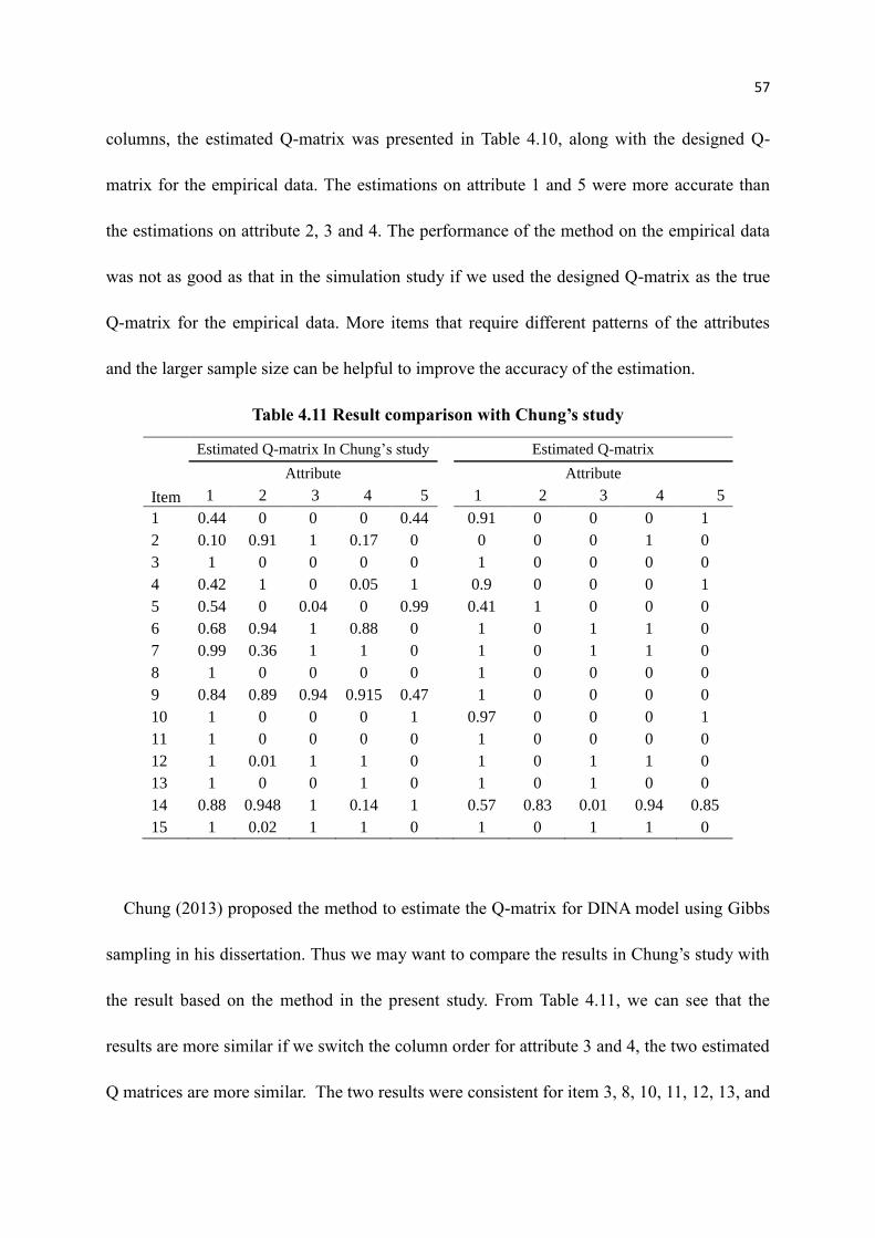
57

columns, the estimated Q-matrix was presented in Table 4.10, along with the designed Q-

matrix for the empirical data. The estimations on attribute 1 and 5 were more accurate than

the estimations on attribute 2, 3 and 4. The performance of the method on the empirical data

was not as good as that in the simulation study if we used the designed Q-matrix as the true

Q-matrix for the empirical data. More items that require different patterns of the attributes

and the larger sample size can be helpful to improve the accuracy of the estimation.

Table 4.11 Result comparison with Chung’s study

Estimated Q-matrix In Chung’s study Estimated Q-matrix

Attribute Attribute

Item 1 2 3 4 5 1 2 3 4 5

1 0.44 0 0 0 0.44 0.91 0 0 0 1

2 0.10 0.91 1 0.17 0 0 0 0 1 0

3 1 0 0 0 0 1 0 0 0 0

4 0.42 1 0 0.05 1 0.9 0 0 0 1

5 0.54 0 0.04 0 0.99 0.41 1 0 0 0

6 0.68 0.94 1 0.88 0 1 0 1 1 0

7 0.99 0.36 1 1 0 1 0 1 1 0

8 1 0 0 0 0 1 0 0 0 0

9 0.84 0.89 0.94 0.915 0.47 1 0 0 0 0

10 1 0 0 0 1 0.97 0 0 0 1

11 1 0 0 0 0 1 0 0 0 0

12 1 0.01 1 1 0 1 0 1 1 0

13 1 0 0 1 0 1 0 1 0 0

14 0.88 0.948 1 0.14 1 0.57 0.83 0.01 0.94 0.85

15 1 0.02 1 1 0 1 0 1 1 0

Chung (2013) proposed the method to estimate the Q-matrix for DINA model using Gibbs

sampling in his dissertation. Thus we may want to compare the results in Chung’s study with

the result based on the method in the present study. From Table 4.11, we can see that the

results are more similar if we switch the column order for attribute 3 and 4, the two estimated

Q matrices are more similar. The two results were consistent for item 3, 8, 10, 11, 12, 13, and

58

15. On other items, Chung’s estimated Q-matrix is more likely to have more entries. For

example, the item 9 requires attribute 1 and 3, and Chung’s estimation on item X showed all

5 attributes were sampled for a big proportion after burn-in.

After the two estimated Q-matrix in Table 4.12 were rounded with 0.5 as the cutoff point,

as shown in Table 4.12, we can compare the log likelihood to evaluate the estimation

accuracy. The function “din” in R package “CDM” (Robitzsch et al., 2014) was used to

calculate the log likelihood values. The log likelihood of the Chung’s Q-matrix is -3426.53,

and the likelihood based on the Q-matrix estimated by the proposed method in the present

data is -3325.73. The likelihood using the designed Q-matrix is lower than the two likelihood

value above, which is -3455.84. Thus under the assumption of DINA model, the designed Q-

matrix did not fit the data as good as the estimated Q-matrix, and the proposed method fit the

data better than Chung’s Q-matrix

Table 4.12 Result comparison with Chung’s study

Estimated Q-matrix In Chung’s study Estimated Q-matrix

Attribute Attribute

Item 1 2 3 4 5 1 2 3 4 5

1 0 0 0 0 0 1 0 0 0 1

2 0 1 1 0 0 0 0 0 1 0

3 1 0 0 0 0 1 0 0 0 0

4 0 1 0 0 1 1 0 0 0 1

5 1 0 0 0 1 1 1 0 0 0

6 1 1 1 1 0 1 0 1 1 0

7 1 0 1 1 0 1 0 1 1 0

8 1 0 0 0 0 1 0 0 0 0

9 1 1 1 1 0 1 0 0 0 0

10 1 0 0 0 1 1 0 0 0 1

11 1 0 0 0 0 1 0 0 0 0

12 1 0 1 1 0 1 0 1 1 0

13 1 0 0 1 0 1 0 1 0 0

14 1 1 1 0 1 1 1 0 1 1

15 1 0 1 1 0 1 0 1 1 0

59

Chapter 5

Discussion

This study presented a method to estimate the Q-matrix for DINA model based on

constrained G-DINA model. The G-DINA model includes a specific parameter for each of the

possible combinations of the attributes. The basic idea of the proposed method was to allow

only one parameter to be non-zero for these attribute combinations. The attributes involved in

the combination are considered as the required attribute for the item. Gibbs sampling steps

were developed, as shown in Chapter 3. The performance of the method was examined with a

simulation study and an empirical study. The results from the simulation study indicated that

the proposed method handled the simulation conditions well. The sample size could impact

the accuracy of the Q-matrix estimation. The bigger the sample size, the better the

performance would be. The correlation among the attributes did not show significant impact

of Q-matrix estimation, given the conditions of sample size. In the empirical study, the

estimate Q-matrix is different from the designed Q-matrix by experts in about one fourth of

the cells. We also compared the data fit of the estimated Q-matrix and the designed Q-matrix

given the observed data, and found that the estimated Q-matrix fit the data better.

5.1 Implication of the study

The cognitive diagnostic models were getting popular over the past several years because

60

of its advantage over the traditional test theories. The traditional test theories estimate one

ability or test score for each examinee, and showed who was doing well and who was not.

Different than the traditional test theories, CDMs do not assign a score, but a profile of

mastered skills. Accordingly, we could know why a certain examinee was not doing well one

the test. With this information the teachers can determine more accurately what to teach and

re-teach for a certain student.

DeCarlo (2012) initiated a Bayesian framework for the research of estimation on Q-matrix,

which was further explored by Chung (2013) on DINA model. The present paper applied

Bayesian method on constrained G-DINA model, and showed that the empirically estimated

Q-matrix had the potential to be a good validation for the Q-matrix designed by experts.

From the simulation study, it was shown that the Q-matrix can be accurately estimated if the

test items covered a variety of item classes. Due to the identification issue, the estimate

outcomes were needed to be permuted manually. The high correlation among the attributes

might make the estimation more difficult, but larger sample size could help to overcome. The

study also showed that it was possible for the estimated Q-matrix to fit the data better than

the designed Q-matrix. In such case, the researcher may consider if the estimated Q-matrix

indicate some other solution of the item where estimated and the designed Q-matrix differ. In

practice the estimated Q-matrix should still be secondary to the expert judgement. It can only

support and validate the designed Q-matrix.

We may envision that in the future researchers would be able to apply the CDMs on the

students’ responses from exams to get the skill profile of each student. The adopted Q-matrix

could be built by comparing the designed Q-matrix and the empirically estimated Q-matrix.

61

Or the researches can get the estimated Q-matrix first, and the received Q-matrix is then

overlaid by experts’ adjustment. The researchers can also evaluate whether adding or

dropping one or more attributes in the Q-matrix is appropriate by comparing the likelihood

values.

5.2 Limitation

The Q-matrix in the simulation study was very regular, as shown below. It covered all the

possible attribute patterns that required three or less attributes, and each attribute was

required by 11 items. However a Q-matrix based on a real test may look different. It is likely

in an exam that attributes are not evenly required by test items, and some attributes are

required by more items than others. It is also possible that some items require the same

pattern of attributes, and these items that are redundant in the attribute patterns tend to give

less additional information for the Q-matrix estimation. Moreover, no items in the simulation

study required more than three attributes, and this may not be the case in the real situation. If

the items in a test require more attributes, the estimation task might be more difficult. Further,

in the empirical study, we observed in the designed Q-matrix that some attributes may usually

be required conditional on other attributes. Thus, some attributes may always show up

together in the test. These issues about the Q-matrix may impact the accuracy of the Q-matrix

estimation.

Simulation study included sample size at 1000 and at 2000. The sample size showed

statistically significant effect on the accuracy of estimation, as shown in Table 4.5 and Table

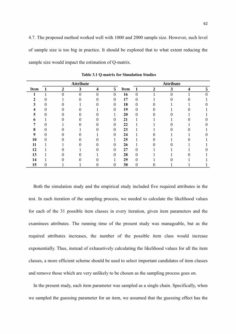
62

4.7. The proposed method worked well with 1000 and 2000 sample size. However, such level

of sample size is too big in practice. It should be explored that to what extent reducing the

sample size would impact the estimation of Q-matrix.

Table 3.1 Q-matrix for Simulation Studies

Attribute Attribute

Item 1 2 3 4 5 Item 1 2 3 4 5

1 1 0 0 0 0 16 0 1 0 1 0

2 0 1 0 0 0 17 0 1 0 0 1

3 0 0 1 0 0 18 0 0 1 1 0

4 0 0 0 1 0 19 0 0 1 0 1

5 0 0 0 0 1 20 0 0 0 1 1

6 1 0 0 0 0 21 1 1 1 0 0

7 0 1 0 0 0 22 1 1 0 1 0

8 0 0 1 0 0 23 1 1 0 0 1

9 0 0 0 1 0 24 1 0 1 1 0

10 0 0 0 0 1 25 1 0 1 0 1

11 1 1 0 0 0 26 1 0 0 1 1

12 1 0 1 0 0 27 0 1 1 1 0

13 1 0 0 1 0 28 0 1 1 0 1

14 1 0 0 0 1 29 0 1 0 1 1

15 0 1 1 0 0 30 0 0 1 1 1

Both the simulation study and the empirical study included five required attributes in the

test. In each iteration of the sampling process, we needed to calculate the likelihood values

for each of the 31 possible item classes in every iteration, given item parameters and the

examinees attributes. The running time of the present study was manageable, but as the

required attributes increases, the number of the possible item class would increase

exponentially. Thus, instead of exhaustively calculating the likelihood values for all the item

classes, a more efficient scheme should be used to select important candidates of item classes

and remove those which are very unlikely to be chosen as the sampling process goes on.

In the present study, each item parameter was sampled as a single chain. Specifically, when

we sampled the guessing parameter for an item, we assumed that the guessing effect has the

63

same distribution regardless the conditional item class. Thus the guessing parameter was

estimated using all the sampled values after burn-in. This method works in the simulation

study because when we simulated the response variable, the guessing parameters of all the

items were set to the same value. A possible alternative method was to sample multiple

chains for the guessing parameter for an item, one for each possible item class. The final

estimation of the guessing parameter should be only based on the samples under the chosen

class of that item. The estimation results based on the two methods may be different if the

item class samples do not converge. However, when the item class converges, the two

methods will be the same.

5.3 Possible topics for future research

The proposed method assumes that the total number of the required attributes was known,

and so the Q-matrix had a fixed number of columns. The next step of the research would be

to determine how many attributes are tested empirically. Such a method may require the

parameter space to vary. For example, if the required attributes increase from five to six, the

possible item classes will change from 31 to 63. It is also necessary to develop some method

to evaluate whether the increasing or decreasing of the Q-matrix column is appropriate. The

reversible jump Markov chain Monte Carlo method (Green, 1995) allows simulation of the

posterior distribution on spaces of varying dimensions, and might be a possible solution for

the task.

Another possible research topic would be relaxing the DINA model assumption when

the Q-matrix is estimated. As discussed in the Chapter 2, DINA model defined the probability

64

of answering the item correctly for only 2 groups, those who mastered all the required

attributes and those who do not. The proposed method estimated the DINA model with

constrained G-DINA model, and so may allow the DINA model assumption to be relaxed. In

the section 3.2, we discussed the possibility of doing this through the G-DINA. For example,

in each iteration we could sample two item classes for item J. The item class with higher

value of probability in posterior distribution was taken as the primary item class, and the Q-

matrix was built based on the samples of the primary item class. At the same time we also

keep the other sampled item class as the secondary item class, which is a possible

combination of attributes with effect on answering the item J. For each primary item class,

we sampled a corresponding attribute effect parameter 𝛾𝑗1; and for each secondary item class,

we sampled a corresponding attribute effect parameter 𝛾𝑗2.

P(𝑋𝑖𝑗 = 1|𝜂𝑖𝑗1, 𝜂𝑖𝑗2) = 𝛾𝑗0 + ∑ 𝐼{𝜏𝑗1=𝑡}2𝐾−1𝑡 =1

𝛾𝑗1𝜂𝑖𝑗1 +∑ 𝐼{𝜏𝑗2=𝑡}

2𝐾−1𝑡 =1

𝛾𝑗2𝜂𝑖𝑗2

= 𝛾𝑗0(1−𝜂𝑖𝑗1)(1−𝜂𝑖𝑗2)(𝛾𝑗0 + 𝛾𝑗1)

𝜂𝑖𝑗1(𝛾𝑗0 + 𝛾𝑗2)(1−𝜂𝑖𝑗1)𝜂𝑖𝑗2

One can also interpret the secondary item class effect as an adjustment to the guessing

parameter. In the section 3.2, the function (3.16) for the relaxed DINA model adopted the

same guessing parameter for all the possible item class. The parameter 𝛾𝑗1 indicates the effect

of mastering all required attributes defined in 𝜂𝑖𝑗1 combination. The 𝛾𝑗2 can be considered as

the adjustment for the guessing effect 𝛾𝑗0 for those who do not master all but a part of the

required attributes. If the sampling results of 𝛾𝑗2 is very different from 0, then we may want

to check the attribute combination defined by 𝜂𝑖𝑗2 because it shows significant effect on

answering the item. If the 𝜂𝑖𝑗2 combination is very different from the 𝜂𝑖𝑗1 combination, it

may imply multiple solutions of the item, which means that it is possible that different

65

combinations of the attribute can equally impact the correctness of the examinee’s answer.

66

Bibliography

Andrieu, C., De Freitas, N., Doucet, A., and Jordan, M. (2004). An introduction to MCMC

for machine learning. Mathine Learning, 50, 5–43.

Birnbaum, A. (1968). Some latent trait models and their use in inferring an examinee’s

ability. Statistical theories of mental test scores. Addison-Wesley Pub. Co.

Casella, G., and George, E. I. (1992). Explaining the Gibbs sampler. The American Statistical

Association, 46, 167–174.

Chen, Y., Liu, J., Xu, G. and Ying, Z. (2015). Statistical analysis of Q-matrix based diagnostic

classification models. Journal of the American Statistical Association, 110, 850-866.

Chen, Y., Liu, J., and Ying, Z. (2015). Online item calibration for Q-matrix in CD-CAT.

Applied Psychological Measurement. 39, 5-15.

Chung, M. (2013). Estimating the Q-matrix for cognitive diagnosis models in a Bayesian

framework. Dissertation.

Cowles, M., & Carlin, B. (1996). Markov Chain Monte Carlo convergence diagnostics: a

comparative review. Journal of the American Statistical Association, 91, 883-904.

de la Torre, J. (2008). An empirically-based method of Q-matrix validation for the DINA

model: Development and applications. Journal of Educational Measurement, 45, 343-

362.

de la Torre, J. (2011). The generalized dina model framework. Psychometrika, 76, 179–199.

de la Torre, J. and Douglas, J. A. (2004). Higher-order latent trait models for cognitive

diagnosis. Psychometrika, 69, 333-353.

de la Torre, J. and Douglas, J. A. (2008). Model evaluation and multiple strategies in

cognitive diagnosis: An analysis of fraction subtraction data. Psychometrika, 73, 595-

624.

67

DeCarlo, L. T. (2010). On the analysis of fraction subtraction data: the DINA model,

classification, latent class sizes, and the Q-matrix. Applied Psychological

Measurement, 35, 8-26.

DeCarlo, L. T. (2012). Recognizing uncertainty in the Q-matrix via a bayesian extension of

the DINA model. Applied Psychological Measurement, 36, 447-468.

DiBello, L., Roussos, L., and Stout, W. (2006). Review of Cognitively Diagnostic

Assessment and a Summary of Psychometric Models. Handbook of statistics, 26, 979

-1030

DiBello, L., Stout, W. F., and Roussor, L. A. (1995). Unified cognitive psychometric

diagnostic assessment likelihood-based classification techniques. Cognitively

diagnostic assessment, Hillsdale, NJ: Erlbaum, 361-389.

Emrich, J. and Piedmonte, M. (1991). A method for generating high-dimensional multivariate

binary variates. The American Statistician, 45, 302–304.

Gelfand, A. and Smith, A. (1990). Sampling based approaches to calculating marginal

densities. American Statistical Association, 85, 398–409.

Gelman, A. and Rubin, D. (1992). Inference from iterative simulation using multiple

sequences. Statistical Science, 7, 457–511.

Geman, S. and Geman, D. (1984). Stochastic relaxation, Gibbs distributions and the Bayesian

restoration of images. IEEE Trans. Pattern Analysis and Machne. Intelligence, 6,

721–741.

Green, P. (1995). Reversible jump Markov chain Monte Carlo computation and Bayesian

model determination, Biometrika, 82, 711-723.

Hambleton, R. and Jones, R. (1993). An NCME instructional module on comparison of

Classical Test Theory and Item Response Theory and their applications to test

development. Educational measurement, issues and practice, 3-38.

Hartz, S. and Roussos, L. (2008). The fusion model for skills diagnosis: blending theory with

practicality. Princeton, NJ: Educational Testing Service.

Hartz, S., Roussos, L., and Stout, W. (2002). Skills diagnosis:Theory and practice. Princeton,

NJ: Educational Testing Service.

Hastings, W. (1970). Monte Carlo sampling methods using Markov chains and their

68

application. Biometrika, 57, 97-109.

Henson, R. A., Templin, J. L., and Willse, J. T. (2009). Defining a family of cognitive

diagnosis models using log-linear models with latent variables. Psychometrika, 74,

191-210.

Huebner, A. (2010). An Overview of Recent Developments in Cognitive Diagnostic

Computer Adaptive Assessments. Practical Assessment, Research & Evaluation, 15,

3.

Im, S. and Corter, J. E. (2011). Statistical consequences of attribute misspecification in the

rule space method. Educational and Psychological Measurement, 71, 712-731.

Junker, B. W. and Sijtsma, K. (2001). Cognitive assessment models with few assumptions,

and connections with nonparametric item response theory. Applied Psychological

Measurement, 25, 258-273.

Lee, Y. W. and Sawaki, Y. (2009). Cognitive diagnosis and Q-matrices in language

assessment. Language Assessment Quarterly, 7, 108-112.

Liu, J., Xu, G. and Ying, Z. (2013). Theory of self-learning Q-matrix. Bernoulli, 19, 1790-

1817.

Liu, J., Xu, G. and Ying, Z. (2012). Data-Driven Learning of Q-Matrix. Applied

Psychological Measurement, 36, 548–564.

Lord, F. (1952). A theory of test scores. Psychometric Monograph, 7.

Maris.E.(1999). Estimating multiple classification latent class models. Psychometrika, 64,

187-212.

Metropolis, N. R. (1953). Equations of state calculations by fast computing machines. J.

Chemical Physics, 21, 1087–1092.

Raftery, A. and Lewis, S. (1992). How many iterations in the Gibbs sampler. Bayesian

Statistics, 4, 763-773.

Robert, C. P. (1995). Convergence control methods for Markov chain Monte Carlo

algorithms. Statistical Science, 10, 231–253.

Robitzsch, A., Kiefer, T. and George, A. C. (2014). CDM: Cognitive Diagnosis Modeling.R

package version 4.1. Retrieved from http://CRAN.R-project.org/package=CDM

69

Rupp, A. and Templin, J. (2008). Effects of Q-matrix misspecification on parameter estimates

and misclassification rates in the DINA model. Educational and Psychological

Measurement, 68, 78–98.

Stephens, M. (1997). Discussion on Bayesian analysis of mixture with an unknown number

of components. Journal of Royal Statistical Society, 59, 768-769.

Stephens, M. (2000). Dealing with label switching in mixtrue models. Journal of Royal

Statistical Society, 62, 795-809.

Tatsuoka, K. (1985). A probabilistic model for diagnosing misconceptions in the pattern

classification approach. Journal of Educational Statistics, 12, 55–73.

Templin, J. (2006). CDM: cognitive diagnosis modeling with Mplus. Retrieved from

http://jtemplin.myweb.uga.edu/cdm/cdm.html

Templin, J. and Henson, R. (2006). Measurement of psychological disorders using cognitive

diagnosis models. Psychological Methods, 11, 287-305.

Von Davier, M. v. (2005). A general diagnostic model applied to language testing data.

Princeton, NJ: Educational Testing Service.

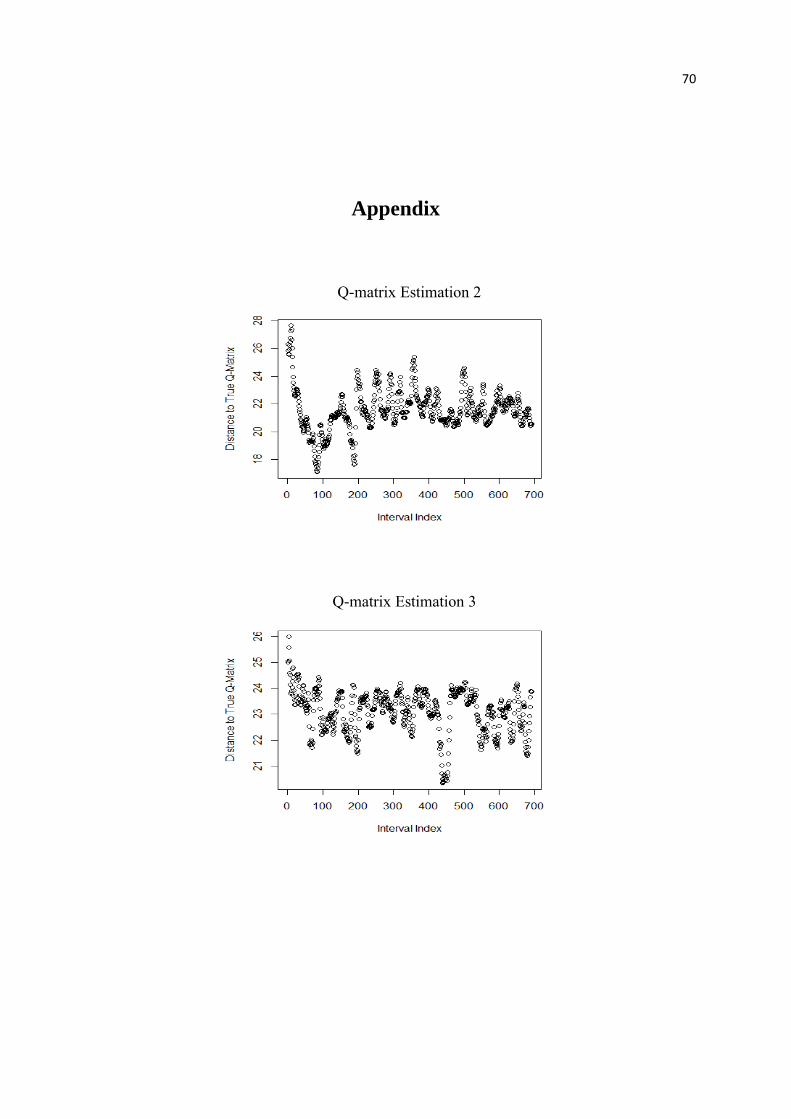
70

Appendix

Q-matrix Estimation 2

Q-matrix Estimation 3

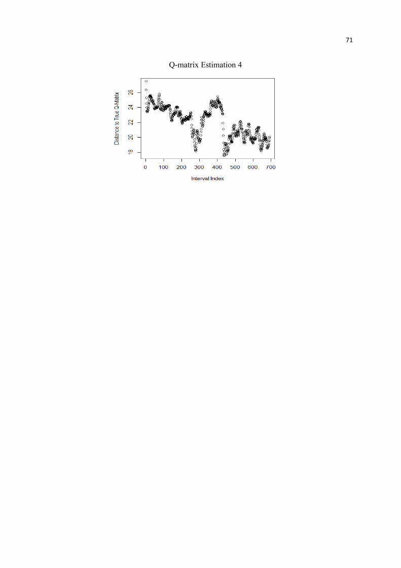
71

Q-matrix Estimation 4