Rank-Constrained Fundamental Matrix Estimation by

Rank-Constrained Fundamental MatrixEstimation by Polynomial Global

Optimization Versus the Eight-PointAlgorithm

Florian Bugarin,1 Adrien Bartoli,2 Didier Henrion,3,4

Jean-Bernard Lasserre,3,5 Jean-Jose Orteu,1 Thierry Sentenac,1,3

February 27, 2014

Abstract

The fundamental matrix can be estimated from point matches. The cur-rent gold standard is to bootstrap the eight-point algorithm and two-viewprojective bundle adjustment. The eight-point algorithm first computes asimple linear least squares solution by minimizing an algebraic cost andthen projects the result to the closest rank-deficient matrix. We propose asingle-step method that solves both steps of the eight-point algorithm. Us-ing recent results from polynomial global optimization, our method finds therank-deficient matrix that exactly minimizes the algebraic cost. In this spe-cial case, the optimization method is reduced to the resolution of very shortsequences of convex linear problems which are computationally efficientand numerically stable. The current gold standard is known to be extremelyeffective but is nonetheless outperformed by our rank-constrained methodfor bootstrapping bundle adjustment. This is here demonstrated on simu-lated and standard real datasets. With our initialization, bundle adjustmentconsistently finds a better local minimum (achieves a lower reprojection er-ror) and takes less iterations to converge.

1Universite de Toulouse; INSA, UPS, Mines Albi, ISAE; ICA (Institut Clement Ader); CampusJarlard, F-81013 Albi, France

2Universite d’Auvergne, ISIT, UMR 6284 CNRS / Universite d’Auvergne, Clermont-Ferrand,France

3LAAS-CNRS, Universite de Toulouse, Toulouse, France4Faculty of Electrical Engineering, Czech Technical University in Prague5Institut de Mathematiques de Toulouse, Universite de Toulouse, Toulouse, France

1

Keywords : Global optimization, linear matrix inequality, fundamentalmatrix.

1 IntroductionThe fundamental matrix has received a great interest in the computer vision com-munity (see for instance (1; 2; 3; 4; 5; 6; 7)). This (3× 3) rank-two matrix en-capsulates the epipolar geometry, the projective motion between two uncalibratedperspective cameras, and serves as a basis for 3D reconstruction, motion segmen-tation and camera self-calibration, to name a few. Given n point matches (qi,q′i),i = 1, . . . ,n between two images, the fundamental matrix may be estimated intwo phases. The initialization phase finds some suboptimal estimate while therefinement phase iteratively minimizes an optimal but nonlinear and nonconvexcriterion. The gold standard uses the eight-point algorithm and projective bun-dle adjustment for these two phases, respectively. A ‘good enough’ initializationis necessary to avoid local minima at the refinement phase as much as possible.The main goal of this article is to improve the current state of the art regardingthe initialization phase. We here focus on input point matches that do not containmismatches (a pair of points incorrectly associated). The problem of mismatcheshas been specifically addressed by the use of robust methods in the literature.

The eight-point algorithm follows two steps (1). In its first step, it relaxes therank-deficiency constraint and solves the following convex problem:

F = argminF∈R3×3

C(F) s.t. ‖F‖2 = 1, (1)

where C is a convex, linear least squares cost, hereinafter called the algebraiccost:

C(F) =n

∑i=1

(q′>i Fqi

)2. (2)

This minimization is subject to the normalization constraint ‖F‖2 = 1. This isto avoid the trivial solution F = 0. Normalization will be further discussed insection 3. The estimated matrix F is thus not a fundamental matrix yet. In itssecond step, the eight-point algorithm computes the closest rank-deficient matrixto F as:

F8pt = argminF∈R3×3

‖F− F‖2 s.t. det(F) = 0. (3)

Both steps can be easily solved. The first step is a simple linear least squaresproblem and the second step is solved by nullifying the least singular value ofF. It has been shown (4) that this simple algorithm performs extremely well in

2

practice, provided that the image point coordinates are standardized by simplyrescaling them so that they lie in [−

√2;√

2]2.Our main contribution in this paper is an approach that solves for the funda-

mental matrix minimizing the algebraic cost. In other words, we find the globalminimum of:

F = argminF∈R3×3

C(F) s.t. det(F) = 0 and ‖F‖2 = 1. (4)

Perhaps more importantly, we also quantify the impact that each of F8pt and F haswhen used as an initial estimate in Bundle Adjustment. Each initial estimate willlead Bundle Adjustment to its own refined estimate. The two final estimates maythus be different since, as the difference between the two initial estimates growslarger, the probability that they lie in different basins of attraction increases. Ourmeasure quantifies:

1. how far are these two basins of attractions,

2. how many iterations will Bundle Adjustment take to converge.

The proposed algorithm uses polynomial global optimization (8; 9). Previous at-tempts (10; 11; 12) in the literature differ in terms of optimization strategy and pa-rameterization of the fundamental matrix. None solves problem (4) optimally fora general parameterization: they either do not guarantee global optimality (11; 12)or prescribe some camera configurations (10; 11; 12) (requiring typically that theepipole in the first camera does not lie at infinity). Furthermore, the main criticismmade to the optimization method we use is the resolution of a hierarchy of con-vex linear problems of increasing size, which is computationally ineffective andnumerically unstable. The proposed solution overcomes this drawback: experi-ments show that, in most of cases, the proposed algorithm only requires solvingthe second relaxation of the sequences used in the exposed optimization method.

Our experimental evaluation on simulated and real datasets compares the dif-ference between the eight-point algorithm and ours used as initialization to bundleadjustment. We observe that (i) bundle adjustment consistently converges withinless iterations with our initialization and (ii) bundle adjustment always achievesan equal or lower reprojection error with our initialization. We provide numerousexamples of real image pairs from standard datasets. They all illustrate practi-cal cases for which our initialization method allows bundle adjustment to reach abetter local minimum than the eight-point algorithm.

3

2 State of the ArtAccurately and automatically estimating the fundamental matrix from a pair ofimages is a major research topic. We first review a four-class categorization of ex-isting methods, and specifically investigate the details of existing global methods.We finally state the improvements brought by our proposed global method.

2.1 Categorizing MethodsA classification of the different methods in three categories –linear, iterative androbust– was proposed in (2). Linear methods directly optimize a linear leastsquares cost. They include the eight-point algorithm (1), SVD resolution (2)and variants (3; 4; 5; 6). Iterative methods iteratively optimize a nonlinear andnonconvex cost. They require, and are sensitive to the quality of, an initial es-timate. The first group of iterative methods minimizes the distances betweenpoints and epipolar lines (13; 14). The second group minimizes some approx-imation of the reprojection error (15; 16; 17; 18). The third group of methodsminimizes the reprojection error, and are equivalent to two-view projective bun-dle adjustment. Iterative methods typically use a nonlinear parameterization ofthe fundamental matrix which guarantees that the rank-deficiency constraint ismet. For instance, a minimal 7-parameter update can be used over a consistentorthogonal representation (7). Finally, robust methods estimate the fundamentalmatrix while classifying each point match as inlier or outlier. Robust methodsuse M-Estimators (19), LMedS (median least squares) (16) or RANSAC (randomsampling consensus) (20). Both LMedS and RANSAC are stochastic.

To these three categories, we propose to add a fourth one: global methods.Global methods attempt at finding the global minimum of a nonconvex prob-lem. Convex relaxations have been used to combine a convex cost with the rank-deficiency constraint (11). However, these relaxations do not converge to a globalminimum and the solution’s optimality is not certified.

2.2 Global MethodsIn theory, for a constrained optimization problem, global optimization methodsdo not require an initial guess and may be guaranteed to reach the global mini-mum, thereby certifying optimality. Such global methods can be separated in twoclasses. The methods of the first class describe the search space as exhaustivelyas possible in order to test as many candidate solutions as possible. Followingthis way, there are methods such as Monte-Carlo sampling, which test random el-ements satisfisying constraints, and reactive tabu search (21; 22), which continuessearching even after a local minimum has been found. The major drawback of

4

these methods is mainly in the prohibitive computation time required to have asufficiently high probability of success. Moreover, even in case of convergence,there is no certificate of global optimality. Contrary to the methods of the firstclass, methods lying in the second class provide a certificate of global optimal-ity using the mathematical theory from which they are built. Branch and Boundalgorithms (23) or global optimization by interval analysis (24; 25) are some ex-amples. However, although these methods can be faster than those of the firstcategory, their major drawback is their lack of generality. Indeed, these meth-ods are usually dedicated to one particular type of cost function because they usehighly specific computing mechanisms to be as efficient as possible. A review ofglobal methods may be found in (26).

A good deal of research has been conducted over the last few decades on ap-plying global optimization methods in order to solve polynomial minimizationproblems under polynomial constraints. The major drawback of these applica-tions has been the difficulty to take constraints into account. But, by solvingsimplified problems, these approaches have mainly been used to find a startingpoint for local iterative methods. However, recent results in the areas of convexand polynomial optimization have facilitated the emergence of new approaches.These have attracted great interest in the computer vision community. In partic-ular, global polynomial optimization (8; 9) has been used in combination witha finite-epipole nonlinear parameterization of the fundamental matrix (10). Thismethod does not consequently cover camera setups where the epipole lies at infin-ity. A global convex relaxation scheme (8; 9) was used to minimize the Sampsondistance (12). Because this implies minimizing a sum of many rational functions,the generic optimization method had to be specifically adapted and lost the prop-erty of certified global optimality.

2.3 The Proposed MethodThe proposed method lies in the fourth category: it is a global method. Simi-larly to the eight-point algorithm, it minimizes the algebraic cost, but explicitlyenforces the nonlinear rank-deficiency constraint. Contrarily to previous globalmethods (10; 11; 12), the proposed method handles all possible camera configu-rations (it does not make an assumption on the epipoles being finite or infinite)and certifies global optimality. Moreover, the presented algorithm is based on theresolution of a very short sequence of convex linear problems and is thereforecomputationally efficient.

A large number of attemps to introduce global optimization have been madein the literature. In (11), a dedicated hierarchy of convex relaxations is definedin order to globally solve the problem of fundamental matrix estimation. Thesingularity constraint is taken into account by introducing additional optimization

5

variables, not introduced directly in the problem description. The resulting opti-mization algorithm is not generic and, contrary to Lasserre’s hierarchy, there isno proof that the sequence of solutions of this specific hierarchy converges to theglobal minimum.

In (10), Lasserre’s hierarchy is used jointly with the introduction of the singu-larity constraint in the problem description. However, the normalization constraint‖F‖2 = 1 is replaced by fixing, a priori, one of the F coefficients to 1. Hence theother F coefficients are not bounded. Consequently, there is no guarantee that thesequence of solutions ( ft)t∈N converges to the global minimum.

In (27) the authors minimize the Sampson distance by solving a specific hi-erarchy of convex relaxations built upon an epigraph formulation. This specifichierarchy is obtained by extending Lasserre’s hierarchy, where the contraints arelinear (LMIs), to a hierarchy of convex relaxations where constraints are polyno-mial (polynomial matrix inequality - PMI). Consequently, no asymptotic conver-gence of the hierarchy to the global optimum can be guaranteed. Moreover, even ifthe rank correction is achieved using the singularity constraint, the normalizationis replaced by setting, a priori, the coefficient f33 to 1 and so the other coefficientsof F are not bounded.

Finally, in a very recent work (28), the algebraic error is globally minimizedthanks to the resolution of seven subproblems. Each subproblem is reduced to apolynomial equation system solved via a Grobner basis solver. The singularityconstraint is satisfied thanks to the right epipole parametrization. Although thisparametrization ensures that F is singular while using the minimum number ofparameters, this method is not practical since it would be necessary to solve 126subproblems in order to cover all the 18 possible parameter sets (16). Thereforeit is preferable to introduce the singularity constraint directly in the problem de-scription rather than via some parametrization of F.

3 Polynomial Global Optimization

3.1 IntroductionGiven a real-valued polynomial f (x) : Rn → R, we are interested in solving theproblem:

f ? = infx∈K

f (x) (5)

where K ⊆ Rn is a (not necessarily convex) compact set defined by polynomialinequalities: g j(x) ≥ 0, j = 1, . . . ,m. Our optimization method is based on an

6

idea first described in (29). It consists in reformulating the nonconvex globaloptimization problem (5) as the equivalent convex linear programming problem:

f = infµ∈P(K)

∫

Kf (x)dµ, (6)

where P(K) is the set of probability measures supported on K. Note that thisreformulation is true for any continuous function (not necessarily polynomial)and any compact set K ⊆ Rn. Indeed, as f ? ≤ f (x), then f ? ≤ ∫K f dµ and thusf ? ≤ f . Conversely, if x? is a global minimizer of (5), then the probability mea-sure µ? M

= δx? (the Dirac at x?) is admissible for (6). Moreover, because f is asolution of (6), the following inequality holds:

∫K f (x)dµ ≥ f , ∀µ ∈ P(K) and

thus f ? =∫

K f (x)δx? ≥ f . Instead of optimizing over the finite-dimensional eu-clidean space K, we optimize over the infinite-dimensional set of probability mea-sures P(K). Thus, Problem (6) is, in general, not easier to solve than Problem (5).However, in the special case of f being a polynomial and K being defined by poly-nomial inequalities, we will show how Problem (6) can be reduced to solving an(generically finite) sequence of convex linear matrix inequality (LMI) problems.

3.2 Notations and DefinitionsFirst, given vectors α = (α1, . . . ,αn)

> ∈Nn and x = (x1, . . . ,xn)> ∈Rn, we define

the monomial xα by:

xα M= xα1

1 xα22 . . .xαn

n (7)

and its degree by deg(xα)M= ‖α‖1 =

n

∑i=1

αi. For t ∈ N, we define Nnt the space of

the n-dimensional integer vector with a norm lower than t as:

Nnt

M= {α ∈ Nn | ‖α‖1 ≤ t} . (8)

Then, consider the family:

{xα}α∈Nnt

={

1,x1,x2, . . . ,xn,x21,x1x2, . . . ,x1xn,x2x3, . . . ,x2

n, . . . ,xt1, . . . ,x

tn}(9)

of all the monomials xα of degree at most t, which has dimension s(t) M=

(n+ t)!t!n!

.

Those monomials form the canonical basis of the vector space Rt [x] of real-valuedmultivariate polynomials of degree at most t. Then, a polynomial p ∈ Rt [x] isunderstood as a linear combination of monomials of degree at most t:

p(x) = ∑α∈Nn

t

pαxα , (10)

7

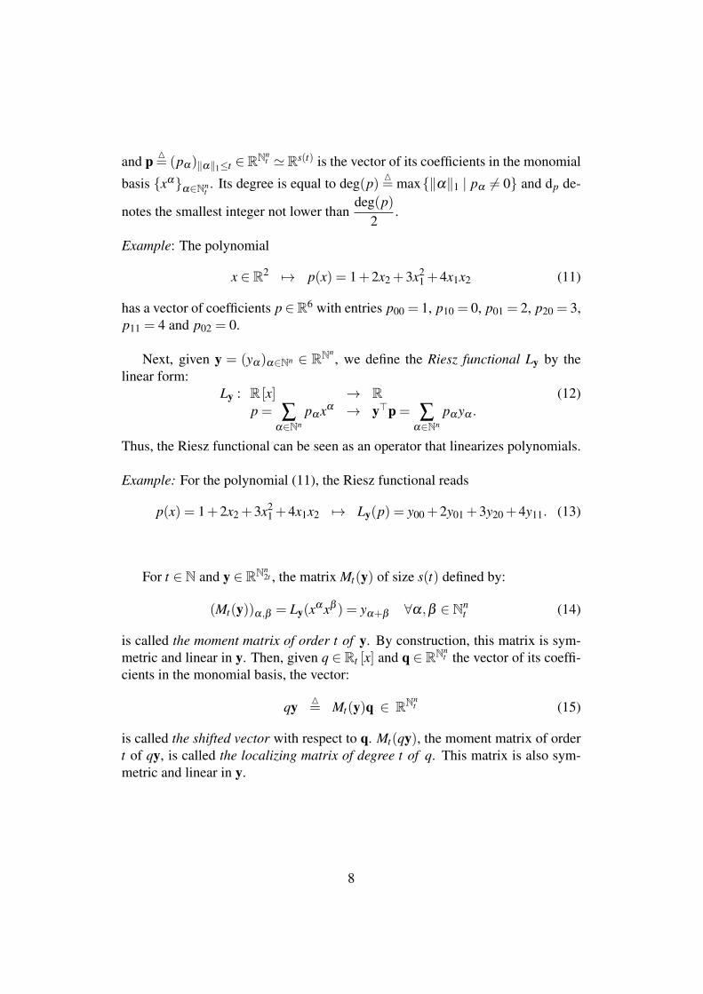
and p M= (pα)‖α‖1≤t ∈RNn

t 'Rs(t) is the vector of its coefficients in the monomial

basis {xα}α∈Nnt. Its degree is equal to deg(p) M

= max{‖α‖1 | pα 6= 0} and dp de-

notes the smallest integer not lower thandeg(p)

2.

Example: The polynomial

x ∈ R2 7→ p(x) = 1+2x2 +3x21 +4x1x2 (11)

has a vector of coefficients p∈R6 with entries p00 = 1, p10 = 0, p01 = 2, p20 = 3,p11 = 4 and p02 = 0.

Next, given y = (yα)α∈Nn ∈ RNn, we define the Riesz functional Ly by the

linear form:Ly : R [x] → R

p = ∑α∈Nn

pαxα → y>p = ∑α∈Nn

pαyα .(12)

Thus, the Riesz functional can be seen as an operator that linearizes polynomials.

Example: For the polynomial (11), the Riesz functional reads

p(x) = 1+2x2 +3x21 +4x1x2 7→ Ly(p) = y00 +2y01 +3y20 +4y11. (13)

For t ∈ N and y ∈ RNn2t , the matrix Mt(y) of size s(t) defined by:

(Mt(y))α,β = Ly(xαxβ ) = yα+β ∀α,β ∈ Nnt (14)

is called the moment matrix of order t of y. By construction, this matrix is sym-metric and linear in y. Then, given q ∈ Rt [x] and q ∈ RNn

t the vector of its coeffi-cients in the monomial basis, the vector:

qy M= Mt(y)q ∈ RNn

t (15)

is called the shifted vector with respect to q. Mt(qy), the moment matrix of ordert of qy, is called the localizing matrix of degree t of q. This matrix is also sym-metric and linear in y.

8

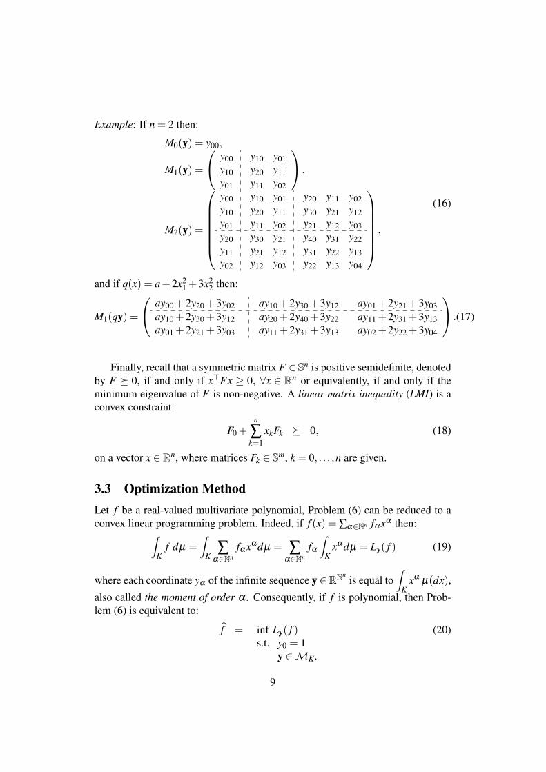
Example: If n = 2 then:

M0(y) = y00,

M1(y) =

y00 y10 y01y10 y20 y11y01 y11 y02

,

M2(y) =

y00 y10 y01 y20 y11 y02y10 y20 y11 y30 y21 y12y01 y11 y02 y21 y12 y03y20 y30 y21 y40 y31 y22y11 y21 y12 y31 y22 y13y02 y12 y03 y22 y13 y04

,

(16)

and if q(x) = a+2x21 +3x2

2 then:

M1(qy) =

ay00 +2y20 +3y02 ay10 +2y30 +3y12 ay01 +2y21 +3y03ay10 +2y30 +3y12 ay20 +2y40 +3y22 ay11 +2y31 +3y13ay01 +2y21 +3y03 ay11 +2y31 +3y13 ay02 +2y22 +3y04

.(17)

Finally, recall that a symmetric matrix F ∈ Sn is positive semidefinite, denotedby F � 0, if and only if x>Fx ≥ 0, ∀x ∈ Rn or equivalently, if and only if theminimum eigenvalue of F is non-negative. A linear matrix inequality (LMI) is aconvex constraint:

F0 +n

∑k=1

xkFk � 0, (18)

on a vector x ∈ Rn, where matrices Fk ∈ Sm, k = 0, . . . ,n are given.

3.3 Optimization MethodLet f be a real-valued multivariate polynomial, Problem (6) can be reduced to aconvex linear programming problem. Indeed, if f (x) = ∑α∈Nn fαxα then:

∫

Kf dµ =

∫

K∑

α∈Nnfαxαdµ = ∑

α∈Nnfα

∫

Kxαdµ = Ly( f ) (19)

where each coordinate yα of the infinite sequence y∈RNnis equal to

∫

Kxα µ(dx),

also called the moment of order α . Consequently, if f is polynomial, then Prob-lem (6) is equivalent to:

f = inf Ly( f )s.t. y0 = 1

y ∈MK.

(20)

9

with:

MKM=

{y ∈ RNn | ∃µ ∈M+(K) such that yα =

∫

Kxαdµ ∀α ∈ Nn

},(21)

andM+(K) is the space of finite Borel measures supported on K. Remark thatthe constraint y0 = 1 is added in order to impose that if y ∈MK then y representsa measure in P(K) (and no longer inM+(K)). Although Problem (20) is a con-vex linear programming problem, it is difficult to describe the convex coneMKwith simple constraints on y. But, the problem “y ∈MK”, also called K-momentproblem, is solved when K is a basic semi-algebraic set, namely:

K M= {x ∈ Rn | g1(x)> 0, . . . ,gm(x)> 0} (22)

where g j ∈R[x], ∀ j = 1, . . .m. Note that K is assumed to be compact. Then, with-out loss of generality, we assume that one of the polynomial inequalities g j(x)> 0is of the form R2−‖x‖2

2 > 0 where R is a sufficiently large positive constant. In thisparticular case,MK can be modelled using LMI conditions on the matrices Mt(y)and Mt(g jy), j = 1, . . .m. More precisely, thanks to the Putinar Theorem (30; 31),we have:

MK = M�(g1, . . . ,gm), (23)

where:

M�(g1, . . . ,gm)M=

{y ∈ RNn|Mt(y)� 0, Mt(g jy)� 0 ∀ j = 1, . . ,m ∀t ∈ N

}.

(24)Then, Problem (6) is equivalent to:

f = infy∈RNn

Ly( f )

s.t. y0 = 1Mt(y)� 0Mt(g jy)� 0 j = 1, . . ,m ∀t ∈ N.

(25)

To summarize, if f is polynomial and K a semi-algebraic set, then Problem (5)is equivalent to a convex linear programming problem with an infinite number oflinear constraints on an infinite number of decision variables. Now, for t ≥ dK

M=

max(d f ,dg1, . . . ,dgm) consider the finite-dimensional truncations of Problem (25):

QtM=

ftM= min

y∈RNn2t

Ly( f )

s.t. y0 = 1Mt(y)� 0,Mt−dg j

(g jy)� 0 ∀ j ∈ {1, . . . ,m} .

(26)

10

By construction, Qt , t ∈ N generates a hierarchy of LMI relaxations of Prob-lem (25) (8), where each Qt , t ∈ N, is concerned with moment and localizingmatrices of fixed size t. Each relaxation (26) can be solved by using public-domain implementations of primal-dual interior point algorithms for semidefiniteprogramming (SDP) (32; 33; 34; 35; 36). When the relaxation order t ∈ N tendsto infinity, we obtain the following results (8; 37):

ft ≤ ft+1 ≤ f and limt→+∞

ft = f . (27)

Practice reveals that this convergence is fast and very often finite, i.e. there ex-ists a finite t0 such that ft = f , ∀t ≥ t0. In fact, finite convergence is guaranteedin a number of cases (e.g. discrete optimization) and very recent results by Nie(37) show that finite convergence is even generic as well as an optimal solution y?tof (26).

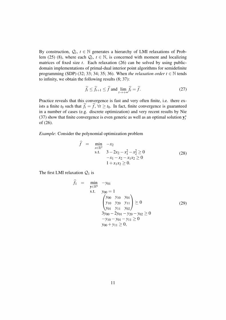
Example: Consider the polynomial optimization problem

f = minx∈R2

−x2

s.t. 3−2x2− x21− x2

2 ≥ 0−x1− x2− x1x2 ≥ 01+ x1x2 ≥ 0.

(28)

The first LMI relaxation Q1 is

f1 = miny∈R6

−y01

s.t. y00 = 1

y00 y10 y01y10 y20 y11y01 y11 y02

� 0

3y00−2y01− y20− y02 ≥ 0−y10− y01− y11 ≥ 0y00 + y11 ≥ 0,

(29)

11

and the second LMI relaxation Q2 is

f2 = miny∈R15

−y01

s.t. y00 = 1

y00 y10 y01 y20 y11 y02y10 y20 y11 y30 y21 y12y01 y11 y02 y21 y12 y03y20 y30 y21 y40 y31 y22y11 y21 y12 y31 y22 y13y02 y12 y03 y22 y13 y04

� 0,

3y00−2y01− y20− y02 3y10−2y11− y30− y12 3y01−2y02− y21− y033y10−2y11− y30− y12 3y20−2y21− y40− y22 3y11−2y12− y31− y133y01−2y02− y21− y03 3y11−2y12− y31− y13 3y02−2y03− y22− y04

� 0

−y10− y01− y11 −y20− y11− y21 −y11− y02− y12−y20− y11− y21 −y30− y21− y31 −y21− y31− y21−y11− y02− y12 −y21− y12− y22 −y12− y03− y13

� 0

y00 + y11 y10 + y21 y01 + y12y10 + y21 y20 + y31 y11 + y22y01 + y12 y11 + y22 y02 + y13

� 0.

(30)It can be checked that f1 = −2 ≤ f2 = f = −1+

√5

2 . Note that the constraint3−2x2− x2

1− x22 ≥ 0 certifies boundedness of the feasibility set.

However, we do not know a priori at which relaxation order t0 the convergenceoccurs. Practically, to detect whether the optimal value is attained, we can useconditions on the rank of the moment and localization matrices. Indeed, let y? ∈RNn

2t be a solution of Problem (26) at a given relaxation order t ≥ dK , if:

rank(Mt(y?)) = rank(Mt−dK(y?)) (31)

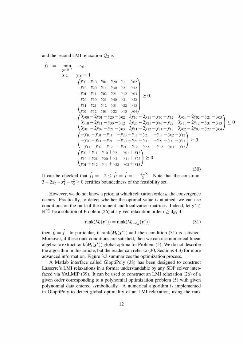
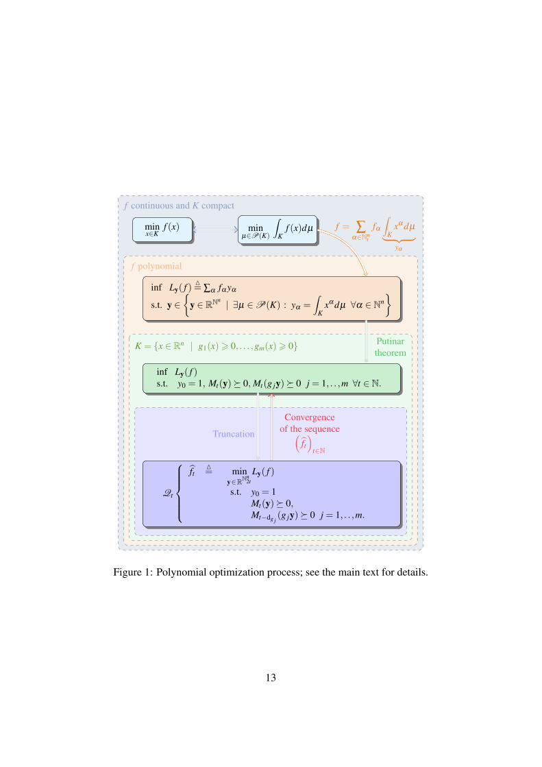
then ft = f . In particular, if rank(Mt(y?)) = 1 then condition (31) is satisfied.Moreover, if these rank conditions are satisfied, then we can use numerical linearalgebra to extract rank(Mt(y?)) global optima for Problem (5). We do not describethe algorithm in this article, but the reader can refer to (30, Sections 4.3) for moreadvanced information. Figure 3.3 summarizes the optimization process.

A Matlab interface called GloptiPoly (38) has been designed to constructLasserre’s LMI relaxations in a format understandable by any SDP solver inter-faced via YALMIP (39). It can be used to construct an LMI relaxation (26) of agiven order corresponding to a polynomial optimization problem (5) with givenpolynomial data entered symbolically. A numerical algorithm is implementedin GloptiPoly to detect global optimality of an LMI relaxation, using the rank

12

minx∈K

f (x) minµ∈P(K)

∫

Kf (x)dµ

inf Ly( f ) M= ∑α fα yα

s.t. y ∈{

y ∈ RNn | ∃µ ∈P(K) : yα =∫

Kxα dµ ∀α ∈ Nn

}

inf Ly( f )s.t. y0 = 1, Mt(y)� 0, Mt(g jy)� 0 j = 1, . . ,m ∀t ∈ N.

Qt

ftM= min

y∈RNn2t

Ly( f )

s.t. y0 = 1Mt(y)� 0,Mt−dg j

(g jy)� 0 j = 1, . . ,m.

f continuous and K compact

f polynomial

K = {x ∈ Rn | g1(x)> 0, . . . ,gm(x)> 0}

f = ∑α∈Nn

t

fα

∫

Kxα dµ

︸︷︷︸yα

Putinartheorem

Truncation

Convergenceof the sequence(

ft)

t∈N

Figure 1: Polynomial optimization process; see the main text for details.

13

tests (31). The algorithm also extracts numerically the global optima from themoment matrix. This approach has been successfully applied to globally solvevarious polynomial optimization problems (see (30) for an overview of resultsand applications). In computer vision this approach was first introduced in (27)and used in (12).

3.4 Application to Fundamental Matrix EstimationAn important feature of our approach is that the singularity constraint can be di-rectly satisfied by our solution and that we do not need an initial estimate as inother methods. Nevertheless, the problem being homogeneous, an additional nor-malization constraint is needed to avoid the trivial solution F= 0. This is generallydone by setting one of the coefficients of the F matrix to 1. However with sucha normalization there is no guarantee that the feasible set is compact which is anecessary condition for the convergence of our polynomial optimization method.Moreover, this normalisation excludes a priori some geometric configurations.Thus, to guarantee compactness of the feasible set and to avoid the trivial solu-tion, we include the additional normalization constraint ‖F‖2 = 1.

Alternatively, the singularity constraint can be inferred by parameterizing theF matrix using one or two epipoles. For instance, in [10] the authors have triedto use polynomial optimization to estimate the F matrix, parametrized by usinga single epipole. However such an approach has several drawbacks. Firstly, thecoefficients of F are not bounded and the convergence of the method is not guaran-teed. Secondly, using the epipole explicitly increases the degree of the polynomialcriterion and consequently, the size of the corresponding relaxations in the hierar-chy. This results in a significant increase of the computational time. Finally, thechoice of this parametrization is arbitrary and does not cover all camera configu-rations.

Our method is summarized in Algorithm 1 below. Its main features are:

• In contrast with (27; 12) the optimization problem is formulated with anexplicit Frobenius norm constraint on the decision variables. This enforcescompactness of the feasibility set which is included in the Euclidean ballof radius 1. We have observed that enforcing this Frobenius norm con-straint has a dramatic influence on the overall numerical behavior of theSDP solver, especially with respect to convergence and extraction of globalminimizers.

• We have chosen the SDPT3 solver (40; 35) since our experiments revealedthat for our problem it was the most efficient and reliable solver.

14

• We force the interior-point algorithm to increase the accuracy as much aspossible, overruling the default parameter set in SDPT3. Then the solverruns as long as it can make progress.

• Generically, polynomial optimization problems on a compact set have aunique global minimizer; this is confirmed in our numerical experimentsas the moment matrix has almost always rank-one (which certifies globaloptimality) at the second SDP relaxation of the hierarchy. In some (veryfew) cases, due to the numerical extraction, the global minimum is not fullyaccurate but yet largely satisfactory.

Algorithm 1 Polynomial optimization for fundamental matrix estimationRequire: Matched points (qi,q′i), i = 1, . . . ,n

1: Create the cost function Crit = ∑ni=1(q′>i Fqi

)2:mpol(’F’,3,3);

for k = 1:size(q1)

n(k) = (q2’*F*q1)^2;

end;

Crit = sum(n);

2: Create the constraints det(F) = 0 and ‖F‖2 = 1:K_det = det(F) == 0; K_fro = trace(F*F’) == 1;

3: Fix the accuracy of the solver to 0, then the solver runs as long as it can makeprogress:pars.eps = 0; mset(pars);

4: Change the default SDP solver to SDPT3:mset(’yalmip’,true); mset(sdpsettings(’solver’,’sdpt3’));

5: Form the second LMI relaxation of the problem:P = msdp(min(crit),K_det,K_fro,2);

6: Solve the second LMI relaxation:msol(P);

4 Experimental ResultsThis section presents results obtained by the test procedure presented below withthe 8-point method and our global method. First, criteria to evaluate the per-formance of a fundamental matrix estimate are described. Next, the evaluationmethodology is detailed. Experiments were then carried out on synthetic data to

15

test the sensitivity to noise and to the number of point matches. Finally, exper-iments on real data were performed to confirm previous results and to study theinfluence of the type ofmotion between the two images.

4.1 Evaluation CriteriaVarious evaluation criteria were proposed in the literature (16) to evaluate thequality of a fundamental matrix estimate. Driven by practice, a fundamental ma-trix estimate F is evaluated with respect to the behavior of its subsequent refine-ment by projective bundle adjustment. Bundle Adjustment from two uncalibratedviews is described as a minimization problem. The cost function is the RMSreprojection errors. The unknowns are the 3D points Qi, i = 1, . . . ,n and the pro-jection matrices P and P′. The criteria we use are:

1. The initial reprojection error written eInit(F).

2. The final reprojection error eBA(F).

3. The number of iterations taken by Bundle Adjustment to converge, Iter(F).

These three criteria assess whether the estimates provided by the two methods,denoted by F8pt and FGp, are in a ‘good’ basin of attraction. Indeed, the num-ber of iterations gives an indication of the distance between the estimate and theoptimum while eBA(F) gives an indication on the quality of the optimum.

4.2 Evaluation MethodThe following algorithm summarizes our evaluation method:

Evaluate(F)

1. Inputs: fundamental matrix estimate F, n point matches (qi,q′i), i= 1, . . . ,n

2. Form initial projective cameras (41):

Find the second epipole from F>e′ ∼ 0(3×1)

Find the canonical plane homography H∗ ∼ [e]×F

Set P∼[I(3×3) 0(3×1)

]and P′ ∼ [H∗ e′]

3. Form initial 3D points (42):

Triangulate each point independently by minimizing the reprojectionerror

16

4. Compute eInit(F)

5. Run two-view uncalibrated bundle adjustment (19)

6. Compute eBA(F) and Iter(F)

7. Outputs: eInit(F), eBA(F) and Iter(F)

4.3 Experiments on Simulated Data4.3.1 Simulation Procedure

For each simulation series and for each parameter of interest (noise, number ofpoints and number of motions), the same methodology is applied with the follow-ing four steps:

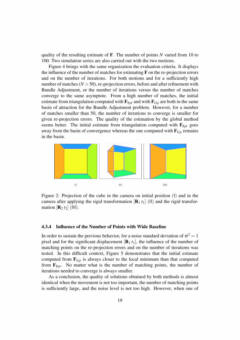
1. For two given motions between two successives images ([Rk tk]) and for agiven matrix K of internal parameters, a set of 3D points (Qi)i, i = 1, . . . ,nis generated and two projection matrices P and P′ are defined. In practice,the rotations matrices, R1 and R2, of two motions are defined by:

RkM=

cos(θk) 0 sin(θk)0 1 0

−sin(θk) 0 cos(θk)

with

θ1 =π3

and

θ2 =π6

(32)

and their translation vectors by t1 = (20,0,5)> and t2 = (6,0,0)>. Thesematrices are chosen such that [R1, t1] is a large movement and [R2, t2] is asmall movement (see Figure 2). We simulated points lying in a cube with10 meter side length. The first camera looks at the center of the cube andit is located 15 meters from the center of the cube. The focal length of thecamera is 700 pixels and the resolution is 640×480 pixels.

2. Thanks to projection matrices P = K [R1, t1] and P′ = K [R2, t2], the set of3D points (Qi)i is projected into the two images as (qi,q′i)i. At each of theirpixel coordinates, a centered Gaussian noise with a variance σ2 is added. Inorder to have statistical evidence, the results are averaged over 100 trials.

3. The resulting noisy points (qi, q′i)i are used to estimate F by our methodFGp and the reference 8-point method F8pt .

4. Finally, via our evaluation procedure we evaluate the estimation error withrespect to the noise standard deviation σ and the number of points n.

17

4.3.2 Sensitivity to Noise

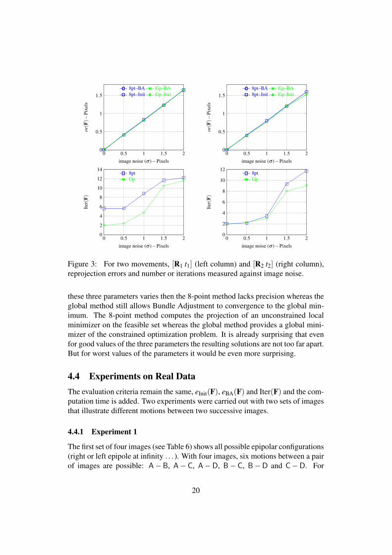
We tested in two simulation series the influence of σ ranging from 0 to 2 pixels.The number of simulated points is 50. The first (resp. second) simulation seriesis based on the first motion [R1 t1] (resp. the second motion [R2 t2]). Figure 3gathers the influence of noise on the evaluation criteria. The first line shows thereproduction errors before, eInit(F), and after eBA(F) refinement through BundleAdjustment with respect to the noise standard deviation. The second line showsthe number of iterations Iter(F) of the Bundle Adjustment versus the noise stan-dard deviation. The first (resp. second) row concerns the first (resp. second)motion.

For the two motions, re-projection errors, eInit(F) or eBA(F), increase with thesame slope when the noise level increases. Notice that for both movements, theBundle-Adjustment step does not improve the results. Indeed, the noise gaussiannoise is added to the projections (qi,q′i)i. So this is noise which in practice wouldbe produced by the extraction points process. Thus the solution produced by theresolution of the linear system is very close to the optimum and does not need tobe refined. The initial solution provided by the triangulation step is then very closeto a local minimum of the Bundle Adjustment problem. Moreover, the variationof the errors of initial re-projection before (8pt − Init and Gp− Init) and after(8pt−BA and Gp−BA) Bundle Adjustment versus the noise standard deviationis linear. However, the number of iterations needed for convergence is differentin the two methods. The initial estimate of the triangulation computed from FGpis closer to the local minimum than that obtained from F8pt . For the first motion(large displacement between camera 1 and 2), the number of iterations of theglobal method (in green) remains smaller than for the 8-point method (in blue)even though their difference seems to decrease when the noise level is high (σ >1). For a significant displacement the quality of the estimate F by the globalmethod remains better even though the difference in quality diminishes with thenoise level. Conversely, for the second motion (small displacement between thecamera 1 and 2) both methods are equivalent since the difference in quality is onlysignificant for a high level of noise (σ > 1). This is logical as the movement is lessimportant. As a conclusion, the 8-point method provides a solution equivalent tothat obtained with the global method when the displacement is not too important.For more significant movements the provided solution is not so close even thoughstill in the same basin of attraction of a local minimum.

4.3.3 Influence of the Number of Points

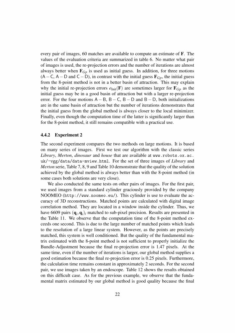
In this experiment, we kept the noise level constant with a standard deviationσ2 = 0.5 pixels. We tested the influence of the number of matches (qi,q′i)i on the

18

quality of the resulting estimate of F. The number of points N varied from 10 to100. Two simulation series are also carried out with the two motions.

Figure 4 brings with the same organization the evaluation criteria. It displaysthe influence of the number of matches for estimating F on the re-projection errorsand on the number of iterations. For both motions and for a sufficiently highnumber of matches (N > 50), re-projection errors, before and after refinement withBundle Adjustment, or the number of iterations versus the number of matchesconverge to the same asymptote. From a high number of matches, the initialestimate from triangulation computed with F8pt and with FGp are both in the samebasin of attraction for the Bundle Adjustment problem. However, for a numberof matches smaller than 50, the number of iterations to converge is smaller forgiven re-projection errors. The quality of the estimation by the global methodseems better. The initial estimate from triangulation computed with F8pt goesaway from the basin of convergence whereas the one computed with FGp remainsin the basin.

Figure 2: Projection of the cube in the camera on initial position (I) and in thecamera after applying the rigid transformation [R1 t1] (II) and the rigid transfor-mation [R2 t2] (III).

4.3.4 Influence of the Number of Points with Wide Baseline

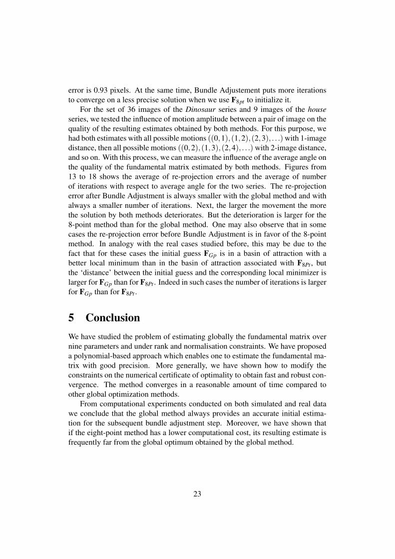
In order to sustain the previous behavior, for a noise standard deviation of σ2 = 1pixel and for the significant displacement [R1 t1], the influence of the number ofmatching points on the re-projection errors and on the number of iterations wastested. In this difficult context, Figure 5 demonstrates that the initial estimatecomputed from FGp is always closer to the local minimum than that computedfrom F8pt . No matter what is the number of matching points, the number ofiterations needed to converge is always smaller.

As a conclusion, the quality of solutions obtained by both methods is almostidentical when the movement is not too important, the number of matching pointsis sufficiently large, and the noise level is not too high. However, when one of

19

0 0.5 1 1.5 20

0.5

1

1.5

image noise (σ ) – Pixels

oe(F)

–Pi

xels

8pt–Init8pt–BA

Gp–InitGp–BA

0 0.5 1 1.5 20

0.5

1

1.5


oe(F)

–Pi

xels

8pt–Init8pt–BA

Gp–InitGp–BA

0 0.5 1 1.5 20

2

4

6

8

10

12

14


Iter(F)

8ptGp

0 0.5 1 1.5 20

2

4

6

8

10

12


Iter(F)

8ptGp

Figure 3: For two movements, [R1 t1] (left column) and [R2 t2] (right column),reprojection errors and number or iterations measured against image noise.

these three parameters varies then the 8-point method lacks precision whereas theglobal method still allows Bundle Adjustment to convergence to the global min-imum. The 8-point method computes the projection of an unconstrained localminimizer on the feasible set whereas the global method provides a global mini-mizer of the constrained optimization problem. It is already surprising that evenfor good values of the three parameters the resulting solutions are not too far apart.But for worst values of the parameters it would be even more surprising.

4.4 Experiments on Real DataThe evaluation criteria remain the same, eInit(F), eBA(F) and Iter(F) and the com-putation time is added. Two experiments were carried out with two sets of imagesthat illustrate different motions between two successive images.

4.4.1 Experiment 1

The first set of four images (see Table 6) shows all possible epipolar configurations(right or left epipole at infinity . . . ). With four images, six motions between a pairof images are possible: A−B, A− C, A−D, B− C, B−D and C−D. For

20

10 20 30 40 50 60 70 80 90 1000.2

0.3

0.4

0.5

Number of points

oe(F)

–Pi

xels

8pt–Init8pt–BA

Gp–InitGp–BA

10 20 30 40 50 60 70 80 90 1000.2

0.3

0.4

0.5

Number of points

oe(F)

–Pi

xels

8pt–Init8pt–BA

Gp–InitGp–BA

10 20 30 40 50 60 70 80 90 1002

3

4

5

6

7

8

9

10

Number of points

Iter(F)

8ptGp

10 20 30 40 50 60 70 80 90 1002

3

4

5

6

Number of points

Iter(F)

8ptGp

Figure 4: For two movements, [R1 t1] (left column) and [R2 t2] (right column),reprojection errors and number or iterations measured against number of pointsfor a gaussian noise with a variance fixed to 0.5.

10 20 30 40 50 60 70 80 90 1000.4

0.6

0.8

1

Number of points

oe(F)

–Pi

xels

8pt–Init8pt–BA

Gp–InitGp–BA

10 20 30 40 50 60 70 80 90 1003456789

101112

Number of points

Iter(F)

8ptGp

Figure 5: For the movement [R1 t1], reprojection errors and number or iterationsmeasured against number of points for a gaussian noise with a variance fixed to 1(left and right).

21

every pair of images, 60 matches are available to compute an estimate of F. Thevalues of the evaluation criteria are summarized in table 6. No matter what pairof images is used, the re-projection errors and the number of iterations are almostalways better when FGp is used as initial guess. In addition, for three motions(A−C, A−D and C−D), in contrast with the initial guess FGp, the initial guessfrom the 8-point method is not in a better basin of attraction. This may explainwhy the initial re-projection errors eInit(F) are sometimes larger for FGp as theinitial guess may be in a good basin of attraction but with a larger re-projectionerror. For the four motions A−B, B−C, B−D and B−D, both initializationsare in the same basin of attraction but the number of iterations demonstrates thatthe initial guess from the global method is always closer to the local minimizer.Finally, even though the computation time of the latter is significantly larger thanfor the 8-point method, it still remains compatible with a practical use.

4.4.2 Experiment 2

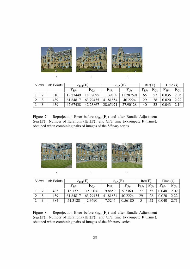
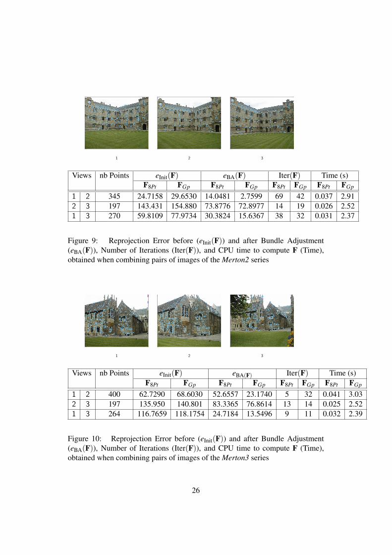
The second experiment compares the two methods on large motions. It is basedon many series of images. First we test our algorithm with the classic seriesLibrary, Merton, dinosaur and house that are available at www.robots.ox.ac.uk/~vgg/data/data-mview.html. For the set of three images of Library andMerton serie, Table 7, 8, 9 and Table 10 demonstrate that the quality of the solutionachieved by the global method is always better than with the 8-point method (insome cases both solutions are very close).

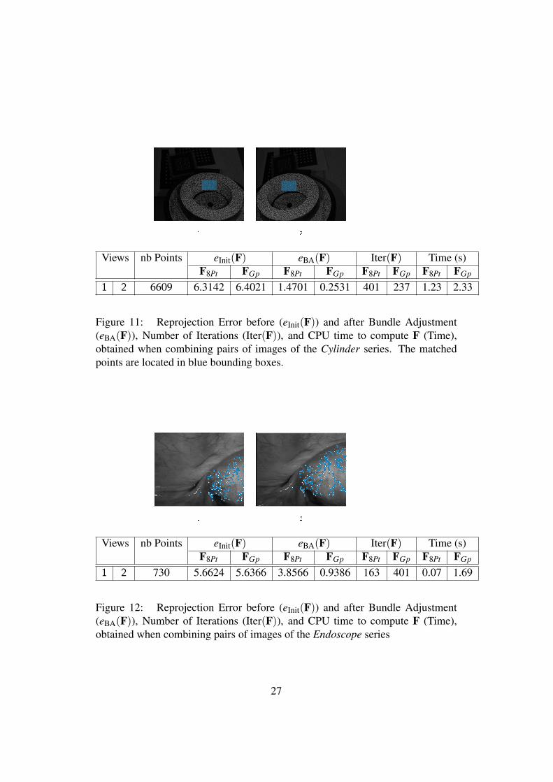
We also conducted the same tests on other pairs of images. For the first pair,we used images from a standard cylinder graciously provided by the companyNOOMEO (http://www.noomeo.eu/). This cylinder is use to evaluate the ac-curacy of 3D reconstructions. Matched points are calculated with digital imagecorrelation method. They are located in a window inside the cylinder. Thus, wehave 6609 pairs (qi,qi)i matched to sub-pixel precision. Results are presented inthe Table 11. We observe that the computation time of the 8-point method ex-ceeds one second. This is due to the large number of matched points which leadsto the resolution of a large linear system. However, as the points are preciselymatched, this system is well conditioned. But the quality of the fundamental ma-trix estimated with the 8-point method is not sufficient to properly initialize theBundle-Adjustment because the final re-projection error is 1.47 pixels. At thesame time, even if the number of iterations is larger, our global method supplies agood estimation because the final re-projection error is 0.25 pixels. Furthermore,the calculation time remains constant in approximately 2 seconds. For the secondpair, we use images taken by an endoscope. Table 12 shows the results obtainedon this difficult case. As for the previous example, we observe that the funda-mental matrix estimated by our global method is good quality because the final

22

www.robots.ox.ac.uk/~vgg/data/data-mview.html

www.robots.ox.ac.uk/~vgg/data/data-mview.html

http://www.noomeo.eu/

error is 0.93 pixels. At the same time, Bundle Adjustement puts more iterationsto converge on a less precise solution when we use F8pt to initialize it.

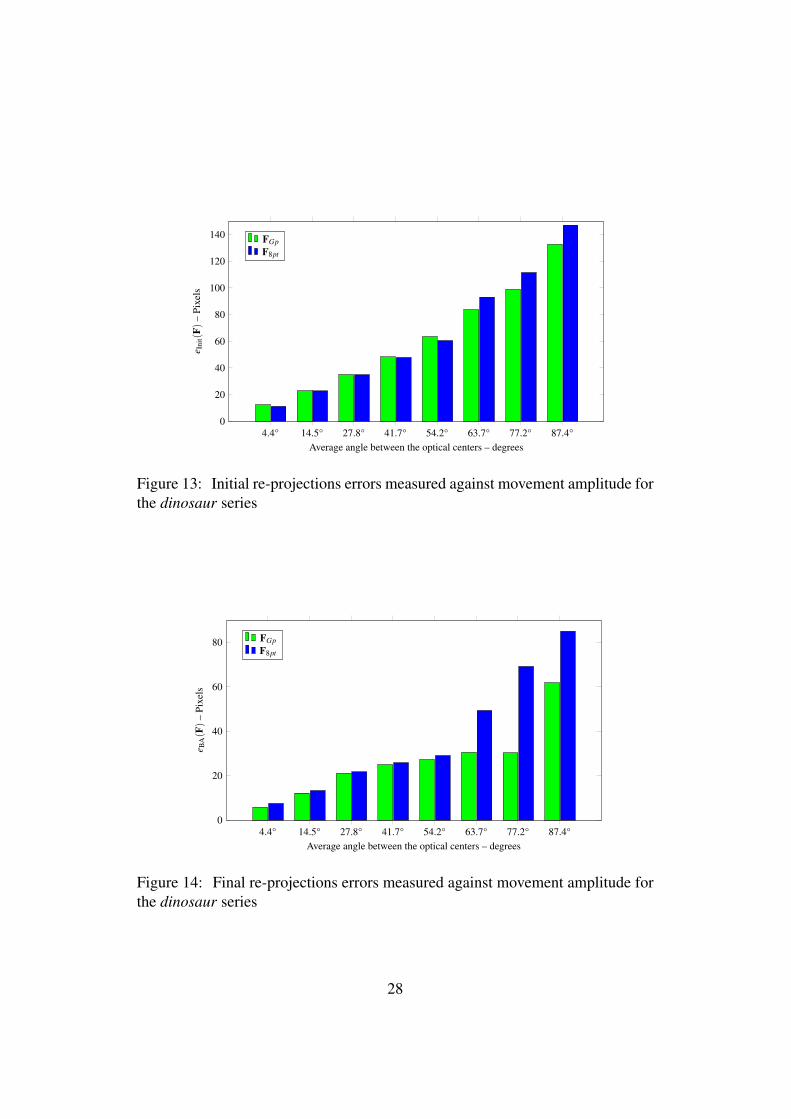
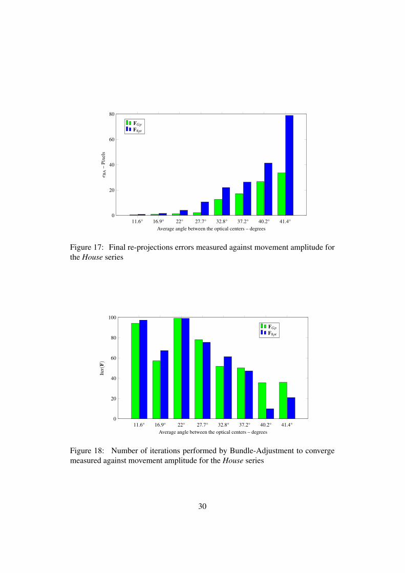
For the set of 36 images of the Dinosaur series and 9 images of the houseseries, we tested the influence of motion amplitude between a pair of image on thequality of the resulting estimates obtained by both methods. For this purpose, wehad both estimates with all possible motions ((0,1),(1,2),(2,3), . . .) with 1-imagedistance, then all possible motions ((0,2),(1,3),(2,4), . . .) with 2-image distance,and so on. With this process, we can measure the influence of the average angle onthe quality of the fundamental matrix estimated by both methods. Figures from13 to 18 shows the average of re-projection errors and the average of numberof iterations with respect to average angle for the two series. The re-projectionerror after Bundle Adjustment is always smaller with the global method and withalways a smaller number of iterations. Next, the larger the movement the morethe solution by both methods deteriorates. But the deterioration is larger for the8-point method than for the global method. One may also observe that in somecases the re-projection error before Bundle Adjustment is in favor of the 8-pointmethod. In analogy with the real cases studied before, this may be due to thefact that for these cases the initial guess FGp is in a basin of attraction with abetter local minimum than in the basin of attraction associated with F8Pt , butthe ‘distance’ between the initial guess and the corresponding local minimizer islarger for FGp than for F8Pt . Indeed in such cases the number of iterations is largerfor FGp than for F8Pt .

5 ConclusionWe have studied the problem of estimating globally the fundamental matrix overnine parameters and under rank and normalisation constraints. We have proposeda polynomial-based approach which enables one to estimate the fundamental ma-trix with good precision. More generally, we have shown how to modify theconstraints on the numerical certificate of optimality to obtain fast and robust con-vergence. The method converges in a reasonable amount of time compared toother global optimization methods.

From computational experiments conducted on both simulated and real datawe conclude that the global method always provides an accurate initial estima-tion for the subsequent bundle adjustment step. Moreover, we have shown thatif the eight-point method has a lower computational cost, its resulting estimate isfrequently far from the global optimum obtained by the global method.

23

— A — — B —

— C — — D —

Views Epipoles eInit(F) eBA(F) Iter(F) Time (s)e e′ F8Pt FGp F8Pt FGp F8Pt FGp F8Pt FGp

A B ∞ ∞ 0.597617 0.65270 0.00252 0.00252 6 6 0.017 2.39A C ∞ ∞ 5.61506 5.61996 2.48258 0.00342 122 175 0.017 1.98A D ∞ ∞ 21.0855 21.5848 4.74837 0.00344 105 30 0.017 2.12B C ∞ ∞ 2.49098 1.91136 0.00260 0.00260 17 12 0.018 1.97B D ∞ ∞ 22.0071 23.6253 0.00268 0.00268 122 81 0.018 1.92C D ∞ ∞ 28.6586 28.6174 16.6507 0.25921 39 1001 0.018 2.1

Figure 6: Reprojection Error before (eInit(F)) and after Bundle Adjustment(eBA(F)), Number of Iterations (Iter(F)), and CPU time to compute F (Time),obtained when combining pairs of images to obtain epipoles close to the imagesor toward infinity

24

1 2 3

Views nb Points eInit(F) eBA(F) Iter(F) Time (s)F8Pt FGp F8Pt FGp F8Pt FGp F8Pt FGp

1 2 310 18.27449 18.32095 11.39809 11.287591 65 57 0.035 2.052 3 439 61.84817 63.79435 41.81854 40.2224 29 28 0.020 2.221 3 439 42.67438 42.23867 28.65971 27.90128 40 32 0.043 2.10

Figure 7: Reprojection Error before (eInit(F)) and after Bundle Adjustment(eBA(F)), Number of Iterations (Iter(F)), and CPU time to compute F (Time),obtained when combining pairs of images of the Library series

1 2 3


1 2 485 15.1771 15.3126 9.8859 9.7360 77 55 0.048 2.022 3 439 61.84817 63.79435 41.81854 40.2224 29 28 0.020 2.221 3 384 51.3128 2.3690 7.5245 0.56180 5 52 0.040 2.71

Figure 8: Reprojection Error before (eInit(F)) and after Bundle Adjustment(eBA(F)), Number of Iterations (Iter(F)), and CPU time to compute F (Time),obtained when combining pairs of images of the Merton1 series

25

1 2 3


1 2 345 24.7158 29.6530 14.0481 2.7599 69 42 0.037 2.912 3 197 143.431 154.880 73.8776 72.8977 14 19 0.026 2.521 3 270 59.8109 77.9734 30.3824 15.6367 38 32 0.031 2.37


1 2 3


1 2 400 62.7290 68.6030 52.6557 23.1740 5 32 0.041 3.032 3 197 135.950 140.801 83.3365 76.8614 13 14 0.025 2.521 3 264 116.7659 118.1754 24.7184 13.5496 9 11 0.032 2.39


26


1 2 6609 6.3142 6.4021 1.4701 0.2531 401 237 1.23 2.33

Figure 11: Reprojection Error before (eInit(F)) and after Bundle Adjustment(eBA(F)), Number of Iterations (Iter(F)), and CPU time to compute F (Time),obtained when combining pairs of images of the Cylinder series. The matchedpoints are located in blue bounding boxes.


1 2 730 5.6624 5.6366 3.8566 0.9386 163 401 0.07 1.69

Figure 12: Reprojection Error before (eInit(F)) and after Bundle Adjustment(eBA(F)), Number of Iterations (Iter(F)), and CPU time to compute F (Time),obtained when combining pairs of images of the Endoscope series

27

4.4° 14.5° 27.8° 41.7° 54.2° 63.7° 77.2° 87.4°0

20

40

60

80

100

120

140

Average angle between the optical centers – degrees

e Ini

t(F)

–Pi

xels

FGpF8pt

Figure 13: Initial re-projections errors measured against movement amplitude forthe dinosaur series

4.4° 14.5° 27.8° 41.7° 54.2° 63.7° 77.2° 87.4°0

20

40

60

80


e BA(F)

–Pi

xels

FGpF8pt

Figure 14: Final re-projections errors measured against movement amplitude forthe dinosaur series

28

4.4° 14.5° 27.8° 41.7° 54.2° 63.7° 77.2° 87.4°0

100

200

300

400


Iter(F)

FGpF8pt

Figure 15: Number of iterations performed by Bundle-Adjustment to convergemeasured against movement amplitude for the dinosaur series

11.6° 16.9° 22° 27.7° 32.8° 37.2° 40.2° 41.4°0

50

100

150

200

250


e Ini

t(F)

–Pi

xels

FGpF8pt

Figure 16: Initial re-projections errors measured against movement amplitude forthe House series

29

11.6° 16.9° 22° 27.7° 32.8° 37.2° 40.2° 41.4°0

20

40

60

80


e BA

–Pi

xels

FGpF8pt

Figure 17: Final re-projections errors measured against movement amplitude forthe House series

11.6° 16.9° 22° 27.7° 32.8° 37.2° 40.2° 41.4°0

20

40

60

80

100


Iter(F)

FGpF8pt

Figure 18: Number of iterations performed by Bundle-Adjustment to convergemeasured against movement amplitude for the House series

30

References[1] H. C. Longuet-Higgins. A computer algorithm for reconstructing a scene

from two projections. Nature, 293:133–135, Sep 1981.

[2] X. Armangue and J. Salvi. Overall view regarding fundamental matrix esti-mation. Image and Vision Computing, 21:205–220, 2003.

[3] R. Y. Tsai and T. S. Huang. Uniqueness and estimation of three-dimensionalmotion parameters of rigid objects with curved surfaces. IEEE Transactionon Pattern Analysis and Machine Intelligence, 6:13–26, 1984.

[4] R. Hartley. In Defence of the 8-point Algorithm. In 5th International Confer-ence on Computer Vision (ICCV’95), pages 1064–1070, Boston (MA, USA),Jun 1995.

[5] P. H. S. Torr and A. W. Fitzgibbon. Invariant fitting of two view geometry or”in defiance of the 8 point algorithm”. 2002.

[6] W. Chojnacki, M. J. Brooks, and A. Van Den Hengel. Revisiting hartley’snormalized eight-point algorithm. IEEE Transactions on Pattern Analysisand Machine Intelligence, 25:1172–1177, 2003.

[7] A. Bartoli and P. Sturm. Nonlinear estimation of the fundamental matrix withminimal parameters. IEEE Trans. Pattern Anal. Mach. Intell., 26(3):426–432, March 2004.

[8] J. B. Lasserre. Global optimization with polynomials and the problem ofmoments. SIAM Journal on Optimization, 11:796–817, 2001.

[9] D. Henrion and J.B. Lasserre. Gloptipoly: Global optimization over poly-nomials with Matlab and SeDuMi. Proceedings of IEEE Conference onDecision and Control, Dec. 2002.

[10] X. Xuelian. New fundamental matrix estimation method using global op-timization. In Proceedings of International Conference on Computer Ap-plication and System Modeling (ICCASM), Taiyuan, China, 22–24 October2010.

[11] G. Chesi, A. Garulli, A. Vicino, and R. Cipolla. Estimating the fundamentalmatrix via constrained least-squares: A convex approach. IEEE Transactionson Pattern Analysis and Machine Intelligence, 24:397–401, 2002.

31

[12] F. Kahl and D. Henrion. Globally optimal estimates for geometric recon-struction problems. International Journal of Computer Vision, 74:3–15,2007.

[13] J. Salvi. An Approach to Coded Structured Light to Obtain Three Dimen-sional Information. PhD thesis, University of Girona, 1999.

[14] P. Chen. Why not use the lm method for fundamental matrix estimation?IET computer vision, 4(4):286–294, 2010.

[15] Q.-T. Luong and O. Faugeras. The fundamental matrix: Theory, algorithms,and stability analysis. International Journal of Computer Vision, 17(1):43–76, 1996.

[16] Z. Zhang. Determining the epipolar geometry and its uncertainty : A review.International Journal of Computer Vision, 27:161–195, 1998.

[17] A. Van Den Hengel, W. Chojnacki, M. J. Brooks, and D. Gawley. A newconstrained parameter estimator: Experiments in fundamental matrix com-putation. In In Proceedings of the 13th British Machine Vision Conference,September 2002.

[18] W. Chojnacki, M. J. Brooks, A. Van Den Hengel, and D. Gawley. A newapproach to constrained parameter estimation applicable to some computervision problems. In Statistical Methods in Video Processing Workshop heldin conjunction with ECCV’02, Copenhagen, Denmark, 2002.

[19] R. Hartley and A. Zisserman. Multiple View Geometry in Computer Vision.Cambridge University Press, 2003.

[20] P. H. S. Torr and D. W. Murray. The development and comparison of robustmethods for estimating the fundamental matrix. International Journal ofComputer Vision, 24:271–300, 1997.

[21] F. Glover. Future paths for integer programming and links to artificial intel-ligence. Comput. Oper. Res., 13(5):533–549, 1986.

[22] P. Hansen and B. Jaumard. Algorithms for the maximum satisfiability prob-lem. Computing, 44(4):279–303, 1990.

[23] A. H. Land and A. G. Doig. An automatic method of solving discrete pro-gramming problems. Econometrica, 28:497–520, 1960.

[24] E. R. Hansen and G. W. Walster. Global optimization using interval analysis,2nd Edn. Marcel Dekker, 2003.

32

[25] R. E. Moore, R. B. Kearfott, and M. J. Cloud. Introduction to Interval Anal-ysis. SIAM, 2009.

[26] T. Weise. Global Optimization Algorithms - Theory and Application.Thomas Weise, 2007-05-01 edition, 2007.

[27] F. Kahl and D. Henrion. Globally optimal estimates for geometric recon-struction problems. In Proc. IEEE Int. Conf. Computer Vision (ECCV), 2005.

[28] Y. Zheng, S. Sugimoto, and M. Okutomi. A practical rank-constrained eight-point algorithm for fundamental matrix estimation. In Computer Vision andPattern Recognition, 2013. CVPR 2013. IEEE Conference on, June 2013.

[29] J. B. Lasserre. Optimisation globale et theorie des moments. Comptes Ren-dus de l’Academie des Sciences, 331:929–934, 2000.

[30] J. B. Lasserre. Moments, positive polynomials and their applications, vol-ume 1 of Imperial College Press Optimization Series. Imperial CollegePress, 2010.

[31] M. Laurent. Sums of squares, moment matrices and optimization over poly-nomials. In Emerging Applications of Algebraic Geometry. IMA Volumes inMathematics and its Applications, 149:157–270, 2009.

[32] B. Borchers. Csdp, a c library for semidefinite programming. OptimizationMethods and Software, 11:613–623, 1999.

[33] S. J. Benson and Y. Ye. DSDP5 user guide — software for semidefinite pro-gramming. Technical Report ANL/MCS-TM-277, Mathematics and Com-puter Science Division, Argonne National Laboratory, Argonne, IL, Septem-ber 2005. http://www.mcs.anl.gov/~benson/dsdp.

[34] K. Fujisawa, M. Fukuda, M. Kojima, K. Nakata, M. Nakata, M. Yamashita,K. Fujisawa, M. Fukuda, and K. Kobayashi. Sdpa (semidefinite program-ming algorithm) – user’s manual. Technical report, Dept. Math. and Comp.Sciences – Tokyo Institute of Technology, 2003.

[35] K.C. Toh, M.J. Todd, and R.H. Tutuncu. Solving semidefinite-quadratic-linear programs using sdpt3. Mathematical Programming, 95:189–217,2003.

[36] J.F. Sturm. Using SeDuMi 1.02, a MATLAB toolbox for optimization oversymmetric cones. Optimization Methods and Software, 11–12:625–653,1999. Version 1.05 available from http://fewcal.kub.nl/sturm.

33

http://www.mcs.anl.gov/~benson/dsdp

[37] J. Nie. Optimality conditions and finite convergence of Lasserre’s hierarchy.Technical report, Dept. Math. – Univ. of California at San Diego, 2012.

[38] D. Henrion, J.B Lasserre, and J. Lofberg. Gloptipoly 3: moments, optimiza-tion and semidefinite programming. Optim. Methods and Software, 24:761–779, 2009.

[39] J. Lfberg. Yalmip : A toolbox for modeling and optimization in MATLAB.In Proceedings of the CACSD Conference, Taipei, Taiwan, 2004.

[40] K.C. Toh, M.J. Todd, and R.H. Tutuncu. Sdpt3 — a matlab software pack-age for semidefinite programming. Optimization Methods and Software,11:545–581, 1999.

[41] Q.-T. Luong and T. Vieville. Canonical representations for the geometriesof multiple projective views. Comput. Vis. Image Underst., 64:193–229,September 1996.

[42] R. Hartley and P. Sturm. Triangulation. Computer Vision and Image Under-standing, 68(2):146–157, 1997.

34

Documents

Rank-Constrained Fundamental Matrix Estimation by