Ann. Inst. Statist. Math. Vol. 46, No. 4, 723-736 (1994)

ESTIMATION OF PARAMETERS IN A TWO-PARAMETER EXPONENTIAL DISTRIBUTION USING RANKED SET SAMPLE

KIN LAM 1, BIMAL K. SINHA 2 AND ZHONG WU 2

1 Department of Statistics, University of Hong Kong, Pokfulam Road, Hong Kong 2 Department of Mathematics and Statistics, University of Maryland Baltimore County,

Baltimore, MD 21228-5398, U.S.A.

(Received June 30, 1993; revised April 28, 1994)

A b s t r a c t . In situations where the experimental or sampling units in a study can be easily ranked than quantified, McIntyre (1952, Aust. J. Agric. Res., 3, 385-390) proposed that the mean of n units based on a ranked set sample (RSS) be used to estimate the population mean, and observed that it provides an unbiased estimator with a smaller variance compared to a simple random sample (SRS) of the same size n. McIntyre's concept of RSS is essentially non- parametric in nature in that the underlying population distribution is assumed to be completely unknown. In this paper we further explore the concept of RSS when the population is partially known and the parameter of interest is not necessarily the mean. To be specific, we address the problem of estimation of the parameters of a two-parameter exponential distribution. It turns out that the use of RSS and its suitable modifications results in much improved estimators compared to the use of a SRS.

Key words and phrases: Best linear unbiased estimator, exponential distribu- tion, order statistics, ranked set sample, uniformly minimum variance unbiased estimator.

1. Introduction

In m a n y sampl ing s i tuat ions when the variable of interest f rom the experi- menta l units can be more easily ranked t h a n quantified, it tu rns out t ha t the use of McIn ty re ' s (1952) not ion of 'Ranked Set Sampling' (RSS) is highly beneficial and much superior to the s t anda rd simple r a n d o m sampl ing (SRS) for es t ima- t ion of the popula t ion mean. Fortunately, in m a n y agricul tural and envi ronmenta l studies, it is indeed possible to rank the exper imenta l or sampl ing units wi thou t ac tual ly measur ing t h e m ra ther cheaply. We refer to Halls and Dell (1966), Mar t in et al. (1980), Cobby et al. (1985) and Sinha et al. (1992) for some applicat ions.

The basic concept behind RSS can be briefly described as follows. Suppose X1, X 2 , . . . , Xn is a r a n d o m sample f rom F(x) with a mean # and a finite var iance ~r 2. Then a s t anda rd nonpa rame t r i c es t imator of p is J~ = E 1 X i / n with v a r ( X ) =

723

724 KIN LAM ET AL.

cr2/n. In contrast to SRS, RSS uses only one observation, namely, Xl:n - X(11), the lowest observation, from this set, then X2:~ -= X(22), the second lowest from another independent set of n observations, and finally X~:n - X(n~), the largest observation from a last set of n observations. This process can be described in Table 1.

Table 1. Display of n 2 observations in n sets of n each•

X(n) X(12) X(21) X(22)

X(~l) X(~2)

• . X(1(~-1)) • . X(2(~-1))

• . X(~(~-I))

xon) x(>~)

X(n~)

The important point to emphasize is that although RSS requires identification of as many as n 2 sampling units, only n of them, namely, {X(n ) , . . . ,X(nn)}, are actually measured, thus making a comparison of this sampling strategy with SRS of the same size n meaningful. Obviously, RSS would be a serious contender to SRS in situations where the task of assembly of the sampling units is easy and their relative rankings in terms of the characteristic under study can be done with negligible cost. It is obvious that the new sample X(n) ,X(22) , . . . ,X(n~) , termed by McIntyre (1952) a Ranked Set Sample (RSS), are independent but not identically distributed. Moreover, marginally, X(ii) is distributed as Xi:~, the i-th order statistic in a sample of size n from F(x). In certain situations, the whole procedure to generate a RSS of size n is repeated m times. Throughout this paper, we consider the case m = 1.

McIntyre (1952) proposed

(1.1) fL~** = ~ X(ii)/n

as a rival estimator of # as opposed to J~. It should be mentioned that McIntyre (1952) gave no supporting mathematical theory to prefer /2~8, over )(. It was provided much later by Takahasi and Wakimoto (1968). It is easy to verify that E(/2~,) = #, and a somewhat surprising result which makes RSS preferable to SRS is that

(1.2) var(ftrs,) < var(X) !

A direct proof of this variance inequality follows from the well-known positively associated property of the order statistics (Tukey (1958), Bickel (1967)). Dell (1969) and Dell and Clutter (1972) provided the following explicit expression for the variance of/2~s where #(0 is the mean of Xi:n.

n (1.3) var(/2~,) = a2 /n - E (#( 0 - #)2/n2.

R A N K E D S E T E S T I M A T I O N F O R E X P O N E N T I A L P A R A M E T E R S 725

Many aspects of RSS have been studied in the literature. Takahasi and Wakimoto (1968) have shown that the relative precision (RP) of/2~** relative to 2 , defined as RP = var(2)/var(/2~s,) , satisfies: 1 _< R P <_ (n + 1)/2, with RP = (n + 1)/2 in case the population is uniform. Patii et al. (1992a) computed the expressions for RP for many discrete and continuous distributions. David and Levine (1972) and Ridout and Cobby (1987) discussed the consequences of presence of errors in ranking. Muttlak and McDonald (1990a, 1990b) developed ranked set sampling theory when the experimental units are selected with size- biased probability with respect to a concomitant variable. Stokes (1980) and Sinha et all (1992) discussed the estimation of variance based on a ranked set sample. Yanagawa and Shirahata (1976) developed RSS theory with selective probability matrix, and Yanagawa and Shan-Huo (1980) discussed the MG-procedure in RSS. For some other aspects of RSS, we refer to Takahashi (1969, 1970), Stokes (1977, 1986), Takahashi and Futatsuya (1988), Kvam and Samaniego (1991) and Patil et al. (1992b).

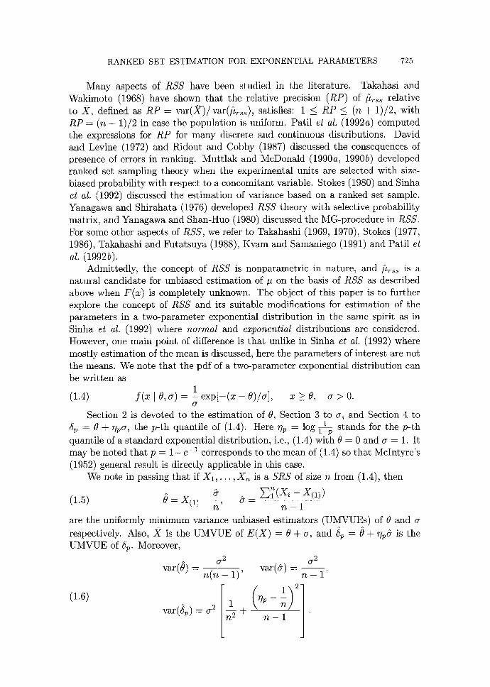
Admittedly, the concept of RSS is nonparametric in nature, and /2~s, is a natural candidate for unbiased estimation of # on the basis of RSS as described above when F(x) is completely unknown. The object of this paper is to further explore the concept of RSS and its suitable modifications for estimation of the parameters in a two-parameter exponential distribution in the same spirit as in Sinha et al. (1992) where normal and exponential distributions are considered. However, one main point of difference is that unlike in Sinha et aI. (1992) where mostly estimation of the mean is discussed, here the parameters of interest are not the means. We note that the pdf of a two-parameter exponential distribution can be written as

1 (1.4) f ( x [ 0, o-) = - exp[ - (x - 0)/o-], x > 0, o- > 0.

a Section 2 is devoted to the estimation of 0, Section 3 to or, and Section 4 to

5p = 0 + %o-, the p-th quantile of (1.4). Here % = log l@p stands for the p-th quantile of a standard exponential distribution, i.e., (1.4) with 0 = 0 and o- = 1. It may be noted that p = 1 - e -1 corresponds to the mean of (1.4) so that McIntyre's (1952) general result is directly applicable in this case.

We note in passing that if X1 , . . . ,X~ is a SRS of size n from (1.4), then

2 ~ ( X i - X ( 1 ) ) (1.5) 0 = 2 ( 1 ) - - - - , ~ =

n n - 1 are the uniformly minimum variance unbiased estimators (UMVUEs) of 0 and respectively. Also, )( is the UMVUE of E ( X ) = 0 ÷ ~, and 5p = 0 ÷ ~p& is the UMVUE of 6p. Moreover,

(1.6)

0-2

n(n - 1)'

I - n2 +

O-2

var(6-) -- n - 1'

726

2. Estimation of 0

K I N L A M E T A L .

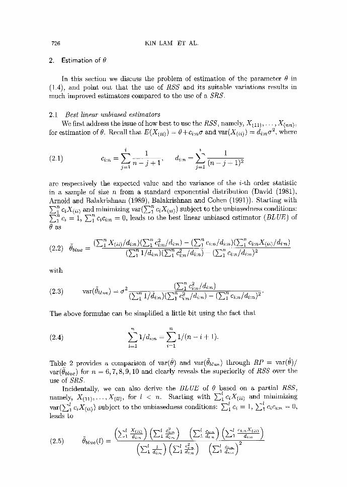
In this section we discuss the problem of est imation of the parameter 0 in (1.4), and point out tha t the use of RSS and its suitable variations results in much improved est imators compared to the use of a SRS.

2.1 Best linear unbiased estimators We first address the issue of how best to use the RSS, namely, X ( 1 1 ) , . . . , X(nn) ,

for est imation of 0. Recall tha t E(X(i~)) = Ù+c~:~cr and var(X(~)) = d~:~a 2, where

i i 1

1 , d i . ~ = E ( n J + l ) 2 (2.1) ei:~ = E n - j + 1 " - j = l j = l

are respectively the expected value and the variance of the i- th order statistic in a sample of size n from a s tandard exponential distr ibution (David (1981), Arnold and Balakrishnan (1989), Balakrishnan and Cohen (1991)). Start ing with ~-~ ciX(ii) and minimizing v a r ( E 1 c~X(.)) subject to the unbiasedness conditions:

n ~-~.1 Ci = I , E n = 1 CiCi:n 0, leads to the best linear unbiased est imator (BLUE) of

0 as

(2.2) Obluc = (~-]l X(ii)/di:n)(Y~-i C2:n/di:n) -- (~-~1 Ci:n/di:n)(E1 Ci:nX(ii)/di:n) 1/di:n)(E 2

with

(2.3) Ci:n/di:n) var(0bl c) = ( E l

n n 2

The above formulae can be simplified a little bit using the fact that

n n

(2.4) E 1/di:n = E 1 / ( n - i + 1). i = 1 i = 1

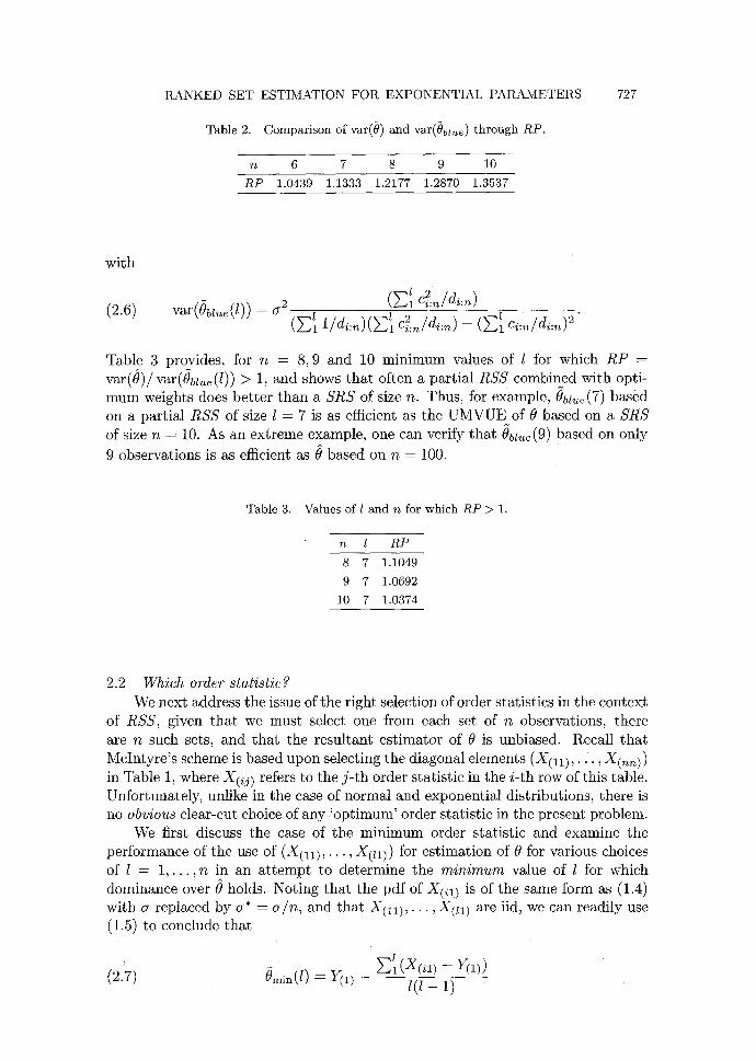
Table 2 provides a comparison of var(0) and var(~)bz~e) through RP = var(0) / var(0blue) for n = 6, 7, 8, 9, 10 and clearly reveals the superiori ty of RSS over the use of SRS.

Incidentally, we can also derive the BLUE of 0 based on a partial RSS, 1 X namely, X O 1 ) , . . . , X ( u ) , for l < n. Start ing with Y~4 ci (ii) and minimizing

var(~l l c~X(ii)) subject to the unbiasedness conditions: E t 1 1 Ci = 1~ E 1 CiCi:n ~- O,

leads to

(2.5) =

R A N K E D SET E S T I M A T I O N F O R E X P O N E N T I A L P A R A M E T E R S

Table 2. Compar ison of var(0) and var(Oblue) t h rough R P .

n 6 7 8 9 10

R P 1.0439 1.1333 1.2177 1.2870 1.3537

727

with

(2.6) -

Table 3 provides, for n = 8, 9 and 10 minimum values of l for which RP = var(~})/var(Oblz¢(1)) > 1, and shows tha t often a partial RSS combined with opti- mum weights does bet ter than a SRS of size n. Thus, for example, 0bl~(7) based on a partial RSS of size l = 7 is as efficient as the UMVUE of 0 based on a SRS of size n = 10. As an extreme example, one can verify tha t 0b~,¢ (9) based on 0nly

9 observations is as efficient as 0 based on n = 100.

Table 3. Values of l and n for which R P > 1.

n l R P

8 7 1.1049

9 7 1.0692

10 7 1.0374

2.2 Which order statistic? We next address the issue of the right selection of order statistics in the context

of RSS, given tha t we must select one from each set of n observations, there are n such sets, and tha t the resultant est imator of 0 is unbiased. Recall tha t McIntyre 's scheme is based upon selecting the diagonal elements (X(11), • . . , X(nn)) in Table 1, where X(ij) refers to the j - t h order statistic in the i- th row of this table. Unfortunately, unlike in the case of normal and exponential distributions, there is no obvious clear-cut choice of any 'opt imum' order statistic in the present problem.

We first discuss the case of the minimum order statistic and examine the performance of the use of (X(11), . . . , X(n)) for est imation of 0 for various choices of I = 1 , . . . , n in an a t t empt to determine the minimum value of l for which dominance over 0 holds. Noting tha t the pdf of X(i!) is of the same form as (1.4) with a replaced by or* = a/n, and tha t X(11), . . . , X(ll) are rid, we can readily use (1.5) to conclude tha t

(2.7) l

Olnin(/) = Y(1) - l(l - 1)

728 KIN L A M E T AL.

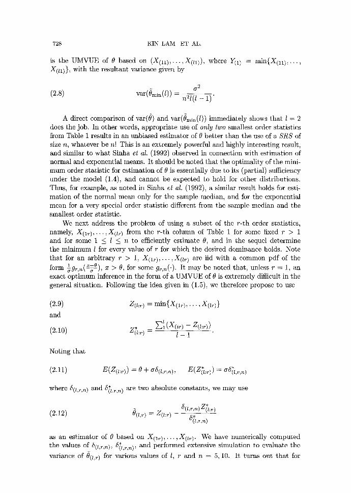
is the UMVUE of 0 based on (X(11),... ,X(ll)), where Y(1) = min{X(m), . . . , X(zl)}, with the resultant variance given by

(y 2

(2.8) var(0mi~(l)) - n21( l _ 1)"

A direct comparison of vat(0) and var(0min(l)) immediately shows that l = 2 does the job. In other words, appropriate use of only two smallest order statistics from Table 1 results in an unbiased estimator of 0 better than the use of a S R S of size n, whatever be n! This is an extremely powerful and highly interesting result, and similar to what Sinha et al. (1992) observed in connection with estimation of normal and exponential means. It should be noted that the optimality of the mini- mum order statistic for estimation of 0 is essentially due to its (partial) sufficiency under the model (1.4), and cannot be expected to hold for other distributions. Thus, for example, as noted in Sinha et al. (1992), a similar result holds for esti- marion of the normal mean only for the sample median, and for the exponential mean for a very special order statistic different from the sample median and the smallest order statistic.

We next address the problem of using a subset of the r-th order statistics, namely, X( l r ) , . . . ,X( t r ) from the r-th column of Table 1 for some fixed r > 1 and for some 1 ~ l < n to efficiently estimate 0, and in the sequel determine the minimum l for every value of r for which the desired dominance holds. Note that for an arbitrary r > 1, X( l r ) , . . . ,X(t~) are iid with a common pdf of the form 1_ ~x-O~ ~g~ ,~[ - -~) , x > 0, for some g~,~(.). It may be noted that, unless r = 1, an exact optimum inference in the form of a UMVUE of 0 is extremely difficult in the general situation. Following the idea given in (1.5), we therefore propose to use

(2.9) and

(2.10)

Z(z:r) = min{X(l r ) , . . . , X(tr) }

1 Z l ( X ( ~ r ) - z(z:r)) Z(l:~) = l - 1

Noting that

(2.11)

where 5(l,r,n ) and 5~z.r,~ ) are two absolute constants, we may use

, (l,~,~) Z(l:~) (2.12) ~(t,~) = Z(z:r) 5"

(Z x,n)

as an estimator of 0 based o n X ( l r ) , . . . , X(Ir) . We have numerically computed the values of 6(t,r,n), 6" and performed extensive simulation to evaluate the (l,r,n)' variance of ~}(t,r) for various values of l, r and n = 5, 10. It turns out that for

R A N K E D S E T E S T I M A T I O N F O R E X P O N E N T I A L P A R A M E T E R S

Table 4.1a. Values of 5(z,2,n ) and 6(*t,2,~) for n = 5.

1 2 3 4 5

5(/,2,n ) .3389 .3511 .3595 .3659

5(/,2,n ) .2806 .2159 .1804 .1573

729

Table 4 . lb . Values of 6(l,2,~ ) and 5~l,2,n ) for n = 10.

l 2 3 4 5 6 7 8 9 10

5(*1,2,n) .1584 .1643 .1683 .1713 .1737 .1756 .1773 .1787 .1799

5(t,2,n ) .1318 .1015 .0848 .0740 .0663 .0605 .0559 .0522 .0491

Table 4.2. S imula t ed values of var(0(/,2 ) ) for n = 5.

l 2 3 4 5

var(0(/,2)) 0.1078(72 0.0368a 2. 0.0191or 2. 0.0128a 2.

~

Table 4.3: S imula ted values of var(O(t,2)) for n = 10.

l 2 3 4 5

var(O(t,2)) 0.i096a 2 0.0372~ 2 0.0192a 2 0.0129cr 2

6 7 8 9 10

0.0092~ 2. 0 .0064a 2. 0.0049~ 2. 0.0042(72* 0.0037c ~2.

~

Table 4.4. S imula ted s t a n d a r d errors of s imu la t ed var(0(l,2)) for n = 5.

l 2 3 4 5

s.e. 6.1074 × 10 -06 3.3474 × 10 -07 5.1550 × 10 -08 1.9139 × 10 - ° s

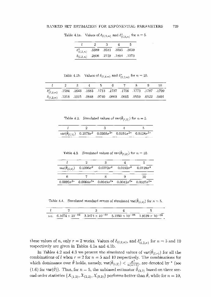
these values of n, only r = 2 works. Values of 5(z,2,,), and 5~1,2,~ ) for n = 5 and 10 respectively are given in Tables 4.1a and 4.lb.

In Tables 4.2 and 4.3 we present the simulated values of var(0(t,r)) for all the combinations of l when r = 2 for n = 5 and 10 respectively. The combinations for

~2 which dominance over 0 holds, namely, var(0(z,2)) < ~(n-1), are denoted by * (see

(1.6) for vat(0)). Thus, for n = 5, the unbiased est imator 0(3,2) based on three sec-

ond order statistics {X(12), X(2,2), X(a,2) } performs bet ter than 0, while for n = 10,

730 KIN LAM E T AL.

the unbiased estimator 4(6,2) based on {X 02), X(2,2), X(a,2), X(<2), X(5,2), X(6,2)}

is better than 0. The simulated values of the variances of 0(l,~) are based on

10,000 replications of the values of 0(l,~), each 0(1,~) in turn being generated from n 2 simulated standard exponential variables.

To examine the stability of the above simulated values, we generated 20 sets of values of simulated var(0(l,2)) for n = 5 and l = 2, 3, 4, 5, each set in turn being based on 10,000 replications of standard exponential variables. The standard errors of these 20 values are given above in Table 4.4. It is clear that the amount of variation is very small, and dominance of 0(t,2) over 0 for n = 5 and 1 > 3 always holds.

3. Estimation of

In this section we discuss the problem of estimation of the parameter cr in (1.4), and point out that the use of RSS and its suitable variations results in much improved estimators compared to the use of a SRS.

3.1 BLUE To derive the BLUE of a based on the entire McIntyre sample X(11), . . . ,

X X(,~,), we minimize the variance of ~--~-i ci (ii) subject to the unbiasedness condi- n tions: ~-~.~ ci = 0, ~ 1 cici:n = 1. This results in

d n n (E~ X(ioci:,~l i:-)(Y~-i l/d~:~) - ( E l c~:nldi:,~)(Y~.l X(ioId~:n) (3.1) ~blue = ( ~ 1 1 / d i : n ) ( ~ l C2:n/di:n) - ( E l n c z n ' : / d , n )

with

(3.2) var(ab,, ) = a 2 ( E l Ci:n/ i:n) (El 2 2 d -

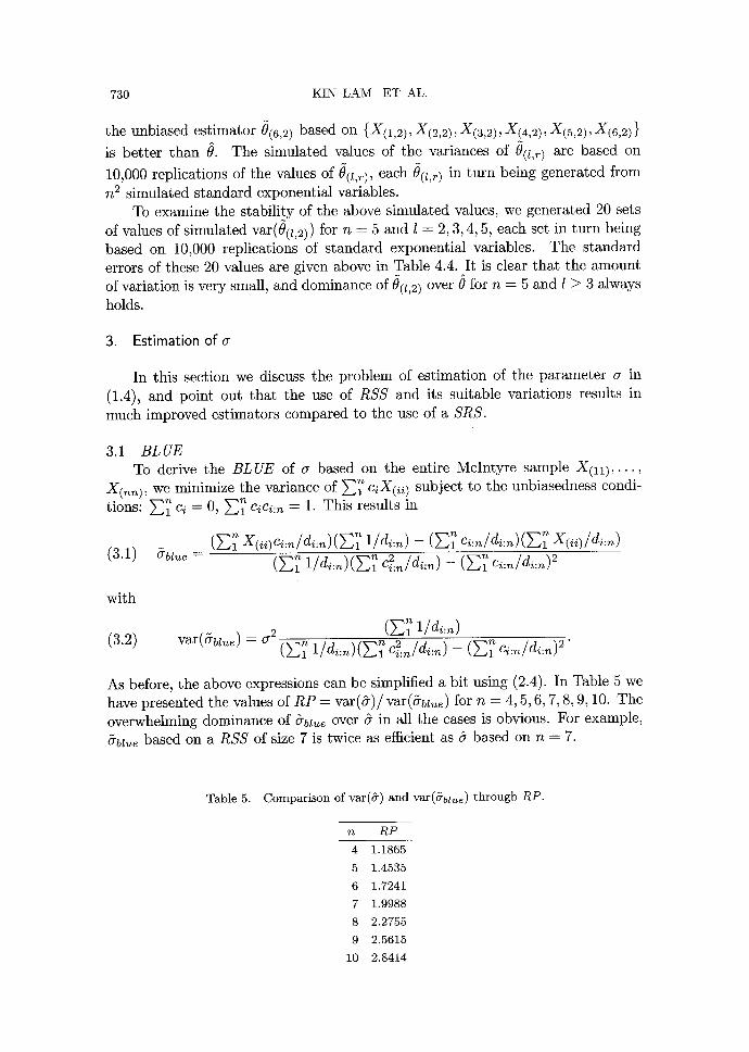
As before, the above expressions can be simplified a bit using (2.4). In Table 5 we have presented the values of RP = var(&)/var(~bt~¢) for n = 4, 5, 6, 7, 8, 9, 10. The overwhelming dominance of 5bt,~ over & in all the cases is obvious. For example, ~bZ~ based on a RSS of size 7 is twice as efficient as a based on n = 7.

Table 5. Compar ison of var(&) and var(&bt~,~) t h rough RP.

n RP 4 1.1865

5 1.4535

6 1.7241

7 1.9988

8 2.2755

9 2.5615

10 2.8414

R A N K E D SET E S T I M A T I O N F O R E X P O N E N T I A L P A R A M E T E R S 731

As in the case of est imation of 0, here also we can use a part ial RSS, namely, X 0 1 ) , . . . , X ( I 0 for some 1 < n. Start ing with }-~,ZlciX(ii) and minimizing

var(}-~ll ciX(ii)) subject to the usual unbiasedness conditions: }-~l 1 ci = 0,

~ l 1 cici:~ = 1, we readily obtain the BLUE of a based on the partial RSS as

l l l d l ( 3 3 ) a l=e(1) = ( E ~ X(<c~:~/d~:~)(E~ 1 / d i : n ) - ( E l Ci:n/ i : n ) ( E 1 X ( i i ) / d i : n )

with

(3.4)

(~-]z 1 1/di:=)(Etl c~:~/di.n) 1 2 • . -- ( E l g i : n / d i : n )

var((rbt~e(1)) = cr 2 (Ell 1/di:n) (El~ 1/d~:~)(El~ c2~:n/d~:n) - (Ell Ci:n/di:n) 2"

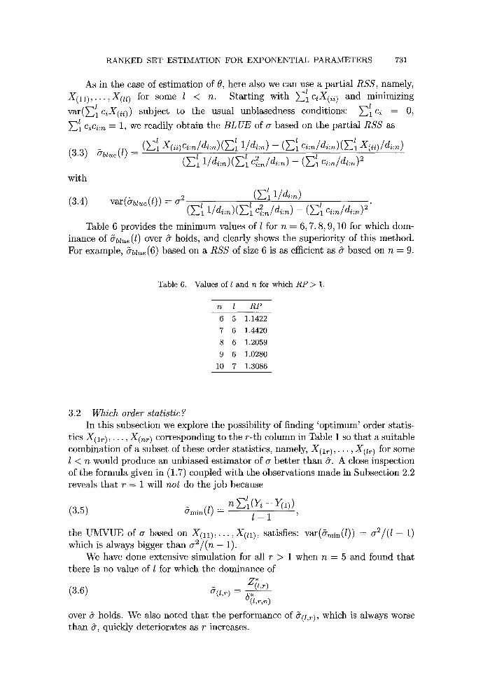
Table 6 provides the minimum values of 1 for n = 6, 7, 8, 9, 10 for which dom- inance of (~bl~e (l) over # holds, and clearly shows the superiority of this method. For example, (~bl~e(6) based on a RSS of size 6 is as efficient as 5 based on n = 9.

Table 6. Values of I and n for which R P > 1.

n l R P

6 5 1.1422

7 6 1.4420

8 6 1.2059

9 6 1.0280

10 7 1.3086

3.2 Which order statistic? In this subsection we explore the possibility of finding 'opt imum' order statis-

tics X(lr), • • . , X(nr) corresponding to the r - th column in Table 1 so tha t a suitable combination of a subset of these order statistics, namely, X 0 r ) , . . . , X(ir) for some 1 < n would produce an unbiased est imator of a bet ter than ~. A close inspection of the formula given in (1.7) coupled with the observations made in Subsection 2.2 reveals tha t r = 1 will not do the job because

EI( - Y(1)) (3.5) ~min(/) = l - 1 '

the UMVUE of a based on X(I~) , . . . ,X(zl), satisfies: var(e~min(/)) = (~2/(1- 1) which is always bigger than a2/(n - 1).

We have done extensive simulation for all r > 1 when n = 5 and found tha t there is no value of 1 for which the dominance of

Z* (l,,) (3.6) 5(z,~)- (5*

(l,r,n)

over 5 holds. We also noted tha t the performance of ~(l,~), which is always worse than ~, quickly deteriorates as r increases.

732 KIN LAM ET AL.

4. Estimation of quantiles

In this section we discuss the problem of estimation of quantiles 5p of (1.4) for various values of 0 < p < 1, and point out that the use of RSS and its suitable variations results in much improved estimators compared to the use of a SRS. The representation of 5p as a linear combination of 0 and cr makes our task quite easy. It should be noted that Stokes and Sager (1988) discussed the nonparametric estimation of a distribution function based on a RSS. However, no such result for estimation of a quantile is available.

4.1 BLUE The BLUE of 5p on the basis of the complete RSS X(11) , . . . , X(n~) can be

derived by minimizing var(~lC~X(~) ) subject to the unbiasedness conditions: }-~.~ ci = 1, ~-~.~ cici:~ = %. This immediately results in

X ( i i ) + A2

1 " 1 "

(4.1)

where

(4.2)

and

- (El ( 4 . 3 ) = -

Moreover, straightforward computations yield

(4.4) var(Sp,bl~) = o 2 E~(c~:~ -- ~P)2/di:~ (E~ 1/d{:~)(E~ c[:,~/d{:~) - ( E ~ c{:~/d{:~) 2"

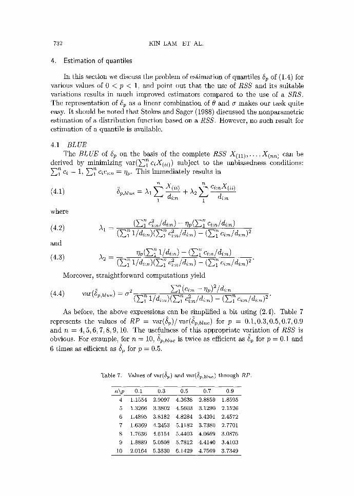
As before, the above expressions can be simplified a bit using (2.4). Table 7

represents the values of RP = var(Sp)/var(Sp,bZ~) for p = 0.1,0.3,0.5,0.7,0.9 and n = 4, 5, 6, 7, 8, 9, 10. The usefulness of this appropriate variation of RSS is obvious. For example, for n : 10, 5p,bt~ is twice as efficient as (~p for p = 0.1 and

6 times as efficient as 5p for p = 0.5.

Table 7. Values of var(Sp) and var(Sp,blue) through R P .

4 1.1554 2.9097 4.3638 2.8859 1.8595

5 1.3266 3.3802 4.5603 3.1290 2.1526

6 1.4895 3.8182 4.8284 3.4201 2.4572

7 1.6369 4.2453 5.1182 3.7380 2.7701

8 1.7636 4.6154 5.4403 4.0669 3.0876

9 1.8889 5.0508 5.7812 4.4140 3.4103

10 2.0164 5.3830 6.1429 4.7569 3.7349

n \ p 0.1 0.3 0.5 0.7 0.9

(4.5)

RANKED SET ESTIMATION FOR E X P O N E N T I A L P A R A M E T E R S 733

Analogously, based on a partial RSS of size l, the BLUE of 5p turns out to be

l l C i : n Z ( i i )

1 di:n 1

where

(4.6)

and

1 2 l ( 2 1 ci:Jdi:n) - ~lp(E1 ci:n/di:n) Al(1) = (E~l 1/d~:n)(Ez 1C2:n/di:n) _ (~-~/1 Ci:n/di:n) 2

(4.7) ~p(~-~.l 1 1/di:~) -(}-~l 1Ci:n/di:n)

A2(I) = (}_~ll 1/d~:n)(}_~ll C2:n/di:n) _ (Ell C i : n / d i : n ) 2 •

Also, direct computations lead to

(4.8) var(Cp,bl,e(/)) = cr 2 }-~Zl ( c i : n - - ? ] p ) 2 / d i : n

(E I - (E I C i : n / d i : n ) 2"

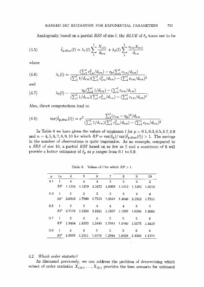
In Table 8 we have given the values of minimum 1 for p = 0.1, 0.3, 0.5, 0.7, 0.9 and n = 4,5,6, 7,8,9,10 for which R P = var(Cp)/var(Cp,bZ~e(l)) > 1. The savings in the number of observations is quite impressive. As an example, compared to a SRS of size 10, a partial RSS based on as few as 2 and a maximum of 6 will provide a better estimator of 5p as p ranges from 0.1 to 0.9.

Table 8. Values of l for which R P > 1.

p \ n 4 5 6 7 8 9 10

0.1 l 4 4 4 3 3 2 2

R P 1.1554 1.1379 1.1672 1.0363 1.1412 1.1250 1.3510

0.3 l 2 2 3 3 3 4 4

R P 2.6916 1.7860 2.7222 1.9824 1.3846 2.1912 1.7211

0.5 l 3 3 4 4 4 5 5

R P 2.7176 1.5283 2.1821 1.5257 1.1205 1.6336 1.3083

0.7 I 3 4 4 5 5 5 6

R P 1.3434 1.8353 1.2440 1.7013 1.3160 1.0575 1.4410

0.9 1 4 4 5 5 6 6 6

R P 1.8595 1.2311 1.6115 1.2394 1.6058 1.3303 1.1273

4.2 Which order statistic? As discussed previously, we can address the problem of determining which

subset of order statistics X( l r ) , . . . , X(zr) provides the best scenario for unbiased

734 KIN LAM ET AL.

est imation of 6p for a given value of p. Obviously, for r = 1, the arguments presented in Subsections 2.2 and 3.2 show that the U M V U E of 5p is given by

(4.9) ~p,min(/) = 0rain(1) + T]pO-min(/)

where 0rain(l) and #rain(l) are given by (2.5) and (3.5) respectively, and conse- quently

(4.10) var(6p,min(/)) = n2/--- ~ + n~p- n 2 ( l - 1)"

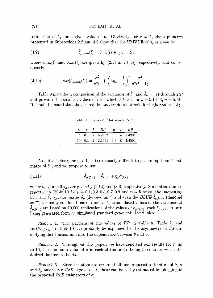
Table 9 provides a comparison of the variances of 6p and 6p,min(/) through R P and provides the smallest values of 1 for which R P > 1 for p = 0.1, 0.3, n = 5, 10. It should be noted that the desired dominance does not hold for higher values of p.

Table 9. Values of l for which RP > 1.

n p l RP p 1 RP

5 0.1 2 5.2802 0.3 4 2.4201 10 0.1 2 2.1961 0.3 8 1.4804

As noted before, for r > 1, it is extremely difficult to get an 'opt imum' esti- mator of 6p, and we propose to use

(4.11)

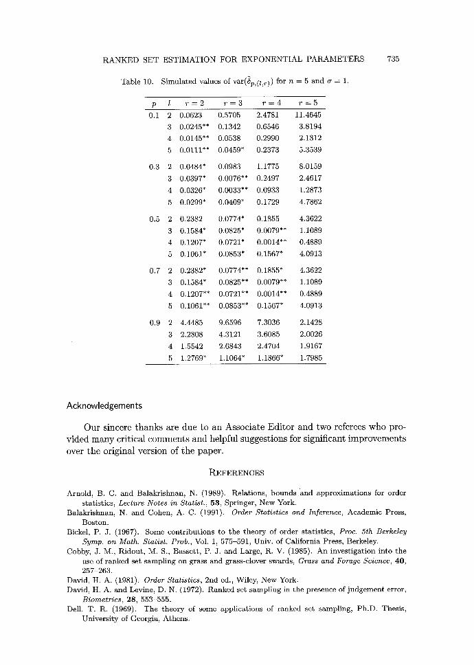
where 0(l,r) and 5(l,r) are given by (2.12) and (3.6) respectively. Simulation studies reported in Table 10 for p = 0.1, 0.3, 0.5, 0.7, 0.9 and n = 5 reveal the interesting fact tha t 6p,(t,r) dominates (~p (denoted as *) and even the B L U E 6p,bl~ (denoted as **) for many combinations of 1 and r. The simulated values of the variances of 6p,(l,~) are based on 10,000 replications of the values of 6p,(t,~), each 6p,(t,~) in turn being generated from n 2 simulated s tandard exponential variables.

R e m a r k 1. The pat terns of the values of R P in Table 8, Table 9, and var(6p,(l,r)) in Table 10 can probably be explained by the a symmet ry of the un-

derlying distr ibution and also the dependence between 0 and ~.

R e m a r k 2. Throughout this paper, we have reported our results for n up to 10, the minimum value of n in each of the tables being the one for which the desired dominance holds.

R e m a r k 3. Since the s tandard errors of all our proposed est imators of 0, and 5p based on a R S S depend on a, these can be easily es t imated by plugging in the proposed R S S estimators of or.

R A N K E D SET ESTIMATION F O R E X P O N E N T I A L P A R A M E T E R S

Simulated values of var(~p,(l,r)) for n = 5 and a = 1. Table 10.

P 0.1

0.3

0.5

0.7

0.9

l r = 2 r----3 r = 4 r = 5

2 0.0623 0.5705 2.4781 11.4645

3 0.0245** 0.1342 0.6546 3.8194

4 0.0145"* 0.0538 0.2990 2.1312

5 0.0111"* 0.0459* 0.2373 5.3539

2 0.0484* 0.0983 1.1775 8.0159

3 0.0397* 0.0076** 0.2497 2.4617

4 0.0326* 0.0033** 0.0933 1.2873

5 0.0299* 0.0409* 0.1729 4.7862

2 0.2382 0.0774* 0.1855 4.3622

3 0.1584" 0.0825* 0.0079** 1.1089

4 0.1207" 0.0721" 0.0014"* 0.4889

5 0.1061" 0.0853* 0.1567" 4.0913

2 0.2382* 0.0774** 0.1855" 4.3622

3 0.1584" 0.0825** 0.0079** 1.1089

4 0.1207"* 0.0721"* 0.0014"* 0.4889

5 0.1061"* 0.0853** 0.1567" 4.0913

2 4.4485 9.6596 7.3036 2.1428

3 2.2808 4.3121 3.6085 2.0026

4 1.5542 2.6843 2.4704 1.9167

5 1.2769" 1.1064" 1.1866" 1.7985

735

A c k n o w l e d g e m e n t s

Our sincere thanks are due to an Associate Editor and two referees who pro- vided many critical comments and helpful suggestions for significant improvements over the original version of the paper.

REFERENCES

Arnold, B. C. and Balakrishnan, N. (1989). Relations, bounds and approximations for order statistics, Lecture Notes in Statist., 53, Springer, New York.

Balakrishnan, N. and Cohen, A. C. (1991). Order Statistics and Inference, Academic Press, Boston.

Bickel, P. J. (1967). Some contributions to the theory of order statistics, Proc. 5th Berkeley Syrup. on Math. Statist. Prob., Vol. 1, 575-591, Univ. of California Press, Berkeley.

Cobby, J. M., Ridout, M. S., Bassett, P. J. and Large, R. V. (1985). An investigation into the use of ranked set sampling on grass and grass-clover swards, Grass and Forage Science, 40, 257-263.

David, H. A. (1981). Order Statistics, 2nd ed., Wiley, New York. David, H. A. and Levine, D. N. (1972). Ranked set sampling in the presence of judgement error,

Biometrics, 28, 553-555. Dell, T. R. (1969). The theory of some applications of ranked set sampling, Ph.D. Thesis,

University of Georgia, Athens.

736 KIN LAM ET AL.

Dell, T. R. and Clutter, J. L. (1972). Ranked set sampling theory with order statistics back- ground, Biometrics, 28, 545 555.

Halls, L. S. and Dell, T. R. (1966). Trial of ranked set sampling for forage yields, Forest Science, 12(1), 22-26.

Kvam, P. H. and Samaniego, F. J. (1991). On the inadmissibility of standard estimators based on ranked set sampling, 1991 Joint Statistical Meetings of ASA Abstracts, 291-292.

Martin, W. L., Sharik, T. L., Oderwald, R. G. and Smith, D. W. (1980). Evaluation of ranked set sampling for estimating shrub phytomass in appalachian Oak forest, Publication No. FWS- 4-80, School of Forestry and Wildlife Resources, Virginia Polytechnic Institute and State University, Blacksburg, Virginia.

McIntyre, G. A. (1952). A method for unbiased selective sampling, using ranked sets, Aust. J. Agric. Res., 3, 385-390.

Muttlak, H. A. and McDonald, L. L. (1990a). Ranked set sampling with respect to concomitant variables and with size biased probability of selection, Comm. Statist. Theory Methods, 19(1), 205-219.

Muttlak, H. A. and McDonald, L. L. (1990b). Ranked set sampling with size biased probability of selection, Biometrics, 46, 435-445.

Patti, G. P., Sinha, A. K. and Taillie, C. (1992a). Ranked set sampling and ecological data analysis, Tech. Reports and Reprints Series, Department of Statistics, Pennsylvania State University.

Patil, G. P., Sinha~ A. K. and Taillie, C. (1992b). Ranked set sampling in the presence of a trend on a site, Tech. Reports and Reprints Series, Department of Statistics, Pennsylvania State University.

Ridout, M. S. and Cobby, J. M. (1987). Ranked set sampling with non-random selection of sets and errors in ranking, Appl. Statist., 36(2), 145-152.

Sinha, B. K., Sinha, B. K. and Purkayastha, S. (1992). On some aspects of ranked set sampling for estimation of normal and exponential parameters (submitted for publication).

Stokes, S. L. (1977). Ranked set sampling with concomitant variables, Comm. Statist. Tneory Methods, 6(12), 1207-1211.

Stokes, S. L. (1980). Estimation of variance using judgment ordered ranked set samples, Bio- metrics, 36, 35-42.

Stokes, S. L. (1986). Ranked set sampling, Encyclopedia of Statistical Sciences, 7 (eds. S. Kotz, N. L. Johnson and C. B. Read), 585-588, Wiley, New York.

Stokes, L. S. and Sager, T. (1988). Characterization of a ranked set sample with application to estimating distribution functions, J. Amer. Statist. Assoc., 83, 374-381.

Takahasi, K. (1969). On the estimation of the population mean based on ordered samples from an equicorrelated multivariate distribution, Ann. Inst. Statist. Math., 21, 249-255.

Takahasi, K. (1970). Practical note on estimation of population means based on samples stratified by means of ordering, Ann. Inst. Statist. Math., 22,421-428.

Takahasi, K. and Futatsuya, M. (1988). Ranked set sampling from a finite population, Proc. Inst. Statist. Math., 36(1), 55-68 (in Japanese).

Takahasi, K. and Wakimoto, K. (1968). On unbiased estimates of the population mean based on the sample stratified by means of ordering, Ann. Inst. Statist. Math., 20, 1 31.

Tukey, J. W. (1958). A problem of Berkson, and minimum variance orderly estimators, Ann. Math. Statist., 29, 588-592.

Yanagawa, T. and Chen, S. H. (1980). The MC-procedure in rank set sampling, J. Statist. Plann. Inference, 4, 33-44.

Yanagawa, T. and Shirahata, S. (1976). Ranked set sampling theory with selective probability matrix, Austral. J. Statist., 18(1, 2), 45-52.