1

Estimation of parameters for the simulation of foam flow through porous media: Part 3; non-uniqueness,

numerical artifact and sensitivity

Kun Maa, Rouhi Farajzadehb, Jose L. Lopez-Salinasa, Clarence A. Millera, Sibani

Lisa Biswala and George J. Hirasakia*

a Department of Chemical and Biomolecular Engineering, Rice University, Houston, TX

77005, USA b Shell Global Solutions International, Rijswijk, The Netherlands

*Corresponding author. Fax: +1 7133485478. Email address: gjh@rice.edu (G. J.

Hirasaki)

Abstract

In the absence of oil in the porous medium, the STARSTM foam model has

three parameters to describe the foam quality dependence, fmmob , fmdry , and

epdry . Even for a specified value of epdry , two pairs of values of fmmob and

fmdry can sometimes match experimentally measured tgf and t

appfoam,µ . This

non-uniqueness can be broken by limiting the solution to the one for which

fmdry < twS . Additionally, a three-parameter search is developed to

simultaneously estimate the parameters fmmob , fmdry , and epdry that fit the

transition foam quality and apparent viscosity. However, a better strategy is to

conduct and match a transient experiment in which 100% gas displaces

surfactant solution at 100% water saturation. This transient scans the entire

range of fractional flow and the values of the foam parameters that best match

2

the experiment can be uniquely determined. Finally, a three-parameter fit using

all experimental data of apparent viscosity versus foam quality is developed.

The numerical artifact of pressure oscillations in simulating this transient

foam process is investigated by comparing finite difference algorithm with

method of characteristics. Sensitivity analysis shows that the estimated foam

parameters are very dependent on the parameters for the water and gas relative

permeability. In particular, the water relative permeability exponent and connate

water saturation are important.

Keywords: foam model; porous media; surfactants; reservoir simulation;

fractional flow theory; mobility control

1. Introduction

Commercial EOR simulators model foam flow with the addition of a mass

balance for surfactant and several factors that describe the reduction in gas

mobility as a function of the dependent variables. The main feature of the

STARSTM foam model (2007 version 1, 2) is the distinction between the low-quality

regime and the high-quality regime in steady-state flow. In the former, the

apparent viscosity increases with increasing foam quality (gas fractional flow)

and in the latter, the apparent viscosity decreases with increasing foam quality.

For a fixed total flow rate, the apparent viscosity is a maximum at this transition.

This transition can be identified by two measurable observations, the transition-

3

fractional flow ( tgf ) and the maximum or transition-apparent viscosity ( t

appfoam,µ ).

In Parts 1 3 & 2 4 of this series of papers we describe how to estimate the

transition from the low-quality to high-quality foam regimes and how to account

for the effects of surfactant concentration and velocity. In this paper we describe

the sensitivity of the model to parameters, numerical oscillations of the transient

foam simulation, possible non-unique solutions, and how the non-uniqueness

can be resolved. The literature survey on modeling foam flow through porous

media was given in Part 1 of this series of papers 3.

2. Results and discussion 2.1 Non-unique solutions to match the transition foam viscosity

2.1.1 Non-graphical solution

In Part 1 of this paper series we introduced a hybrid contour plot method to

match the transition foam viscosity between the high-quality regime and the low-

quality regime. Here we discuss how to solve this problem non-graphically and

how to deal with the issue of non-uniqueness. The equations used for steady-

state modeling of foam flow are shown in the appendix (Eqns (A.1) to (A.5)).

The transition water saturation twS between the high-quality and low-quality

foam regimes is defined by:

),,(max),,( ,, fmdryfmmobSfmdryfmmobS wappfoamS

twappfoam

w

µµ = ................................…(1)

4

With a preset value of epdry , the goal is to solve Eqns (2) and (3) simultaneously

to obtain fmmob and fmdry .

g

tw

frg

w

twrw

tappfoam fmdryfmmobSkSk

µµ

µ),,()(

1,

+

= ………………..….………………….…....(2)

),,()(1

1

fmdryfmmobSkSk

f

tw

frg

g

w

twrw

tg µ

µ⋅+

= ..................................................................(3)

We show how to match the experimental data of 0.2 wt% IOS1518 at the

transition foam quality ( 5.0)( =measuredf tg and cpmeasuredt

appfoam 421)(, =µ ) using

the parameters listed in Table A1 as an example. If the solution exists, one can

use the derivative method and the root-finding algorithm to solve Eqns (1) to (3).

However, a modern strategy is to use search algorithms for finding minimum

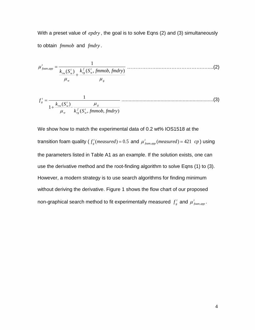
without deriving the derivative. Figure 1 shows the flow chart of our proposed

non-graphical search method to fit experimentally measured tgf and t

appfoam,µ .

5

As shown in Figure 1, this approach uses the simplex search method (the

built-in function “fminsearch” in MATLAB 5) to find fmmob and fmdry and the

golden section search method (the built-in function “fminbnd” in MATLAB 5)

inside the simplex search loop to find twS . The objective functions ( 1Fun and

2Fun ) for minimization using the simplex search in the outer loop and the golden

section search in the inner loop are shown in Eqns (4) and (5), respectively:

22

,

,,1 )(

)()(

)(),(min

−+

−=

measuredfmeasuredff

measuredmeasured

fmdryfmmobFun tg

tg

tg

tappfoam

tappfoam

tappfoam

µµµ

.

..............................................................................................................................(4)

Figure 1. Flow chart of the non-graphical approach to match experimental data at the transition foam quality with a preset epdry .

6

)()(min ,2 wappfoamw SSFun µ−= ..................................................................................(5)

Using an initial guess of 10000=fmmob and 1.0=fmdry , we obtain

47196=fmmob and 1006.0=fmdry with a preset epdry of 500. This result is

consistent with the solution obtained through the hybrid contour plot method in

Part 1 of this series of papers 3 if the difference in significant digits is considered.

2.1.2 Strategy to handle the non-uniqueness problem

The success using the approach proposed in Section 2.1.1 highly depends

on the initial guess of fmmob and fmdry . For example, if we use an initial guess

of 610=fmmob and 1.0=fmdry , the algorithm ends up with a solution of

6101.0897×=fmmob and 1216.0=fmdry . This set of solution can also match the

experimental data at the transition foam quality.

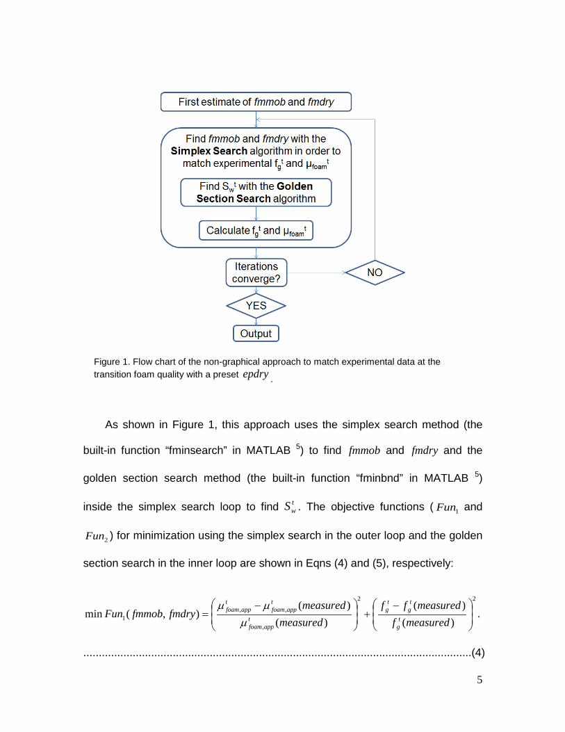
It is necessary to use the graphical method to investigate the existence and

uniqueness of the solutions. As stated in Part 1 of this paper series, the solution

can be found by superimposing the contour plots of the transition foam quality

and the foam apparent viscosity 3. However, only the value of 0.1006 for fmdry

was observed in our previous work due to the limited parameter domain which

had been scanned. In Figure 2(a), we scan the parameter domains for fmmob

over 4 orders of magnitude (103 to 107). Interestingly, the second solution is

found as the contour of the transition foam quality (the red curve in Figure 2)

forms a circuitous curve instead of a monotonic decreasing curve. These two

pairs of solutions for fmmob and fmdry , as indicated by the intersections

7

between the blue curve and the red curve in Figure 2(a), are consistent with the

finding in Figure 1 using the non-graphical method and appropriate starting

values of the parameters.

8

(a)

(b)

Figure 2. Location of the roots which match transition foam data using the hybrid contour plot method on a log-log scale. (a) shows the parameter scan in the range of

73 1010 << fmmob and 10 << fmdry ; (b) shows part of Figure 2(a) where fmdry is

smaller than twS . The rest of the parameters are used as shown in Table A1 with a preset

epdry of 500. The purple dots in both figures indicate where 5.0=tgf (the red curve) and

cptappfoam 421, =µ (the blue curve) cross over.

421cp

421cp

9

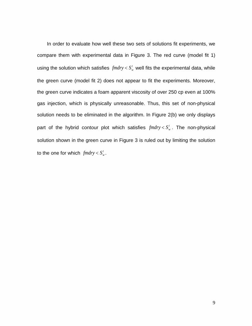
In order to evaluate how well these two sets of solutions fit experiments, we

compare them with experimental data in Figure 3. The red curve (model fit 1)

using the solution which satisfies twSfmdry < well fits the experimental data, while

the green curve (model fit 2) does not appear to fit the experiments. Moreover,

the green curve indicates a foam apparent viscosity of over 250 cp even at 100%

gas injection, which is physically unreasonable. Thus, this set of non-physical

solution needs to be eliminated in the algorithm. In Figure 2(b) we only displays

part of the hybrid contour plot which satisfies twSfmdry < . The non-physical

solution shown in the green curve in Figure 3 is ruled out by limiting the solution

to the one for which twSfmdry < .

10

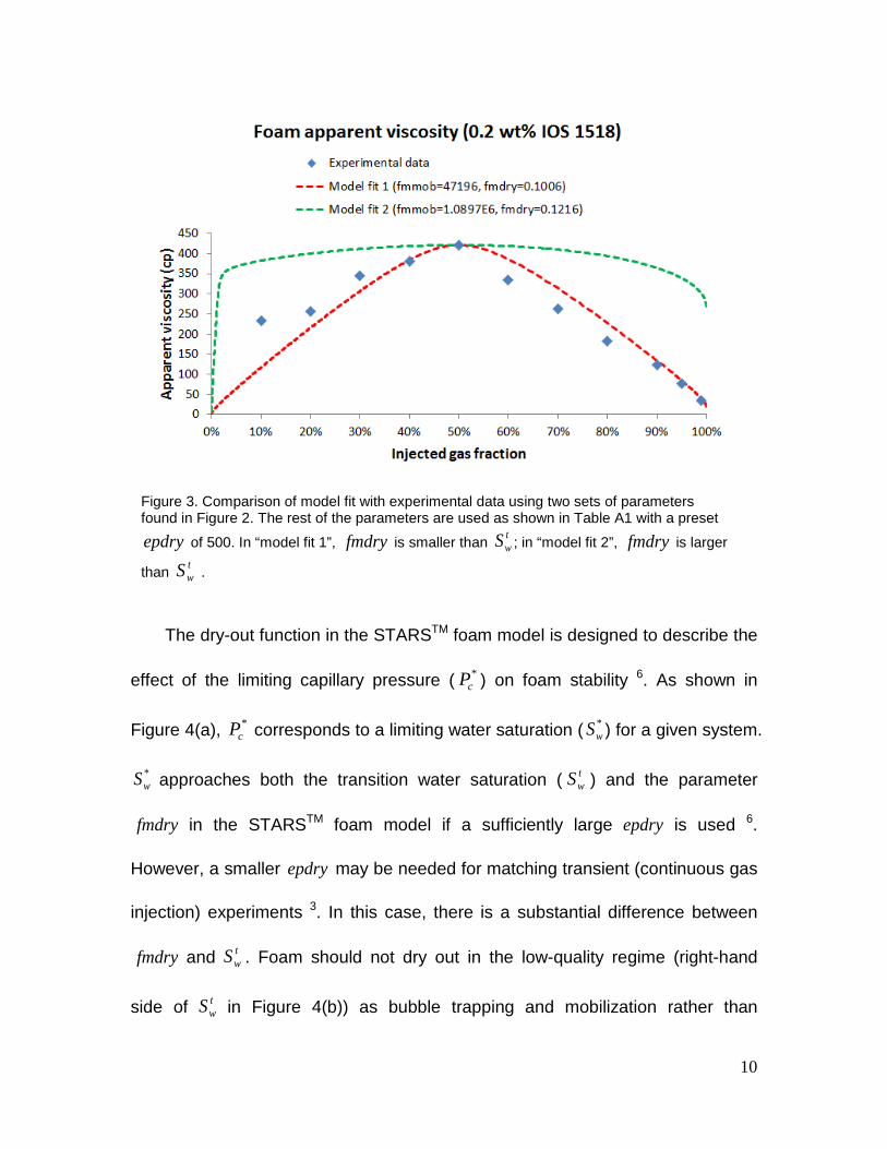
The dry-out function in the STARSTM foam model is designed to describe the

effect of the limiting capillary pressure ( *cP ) on foam stability 6. As shown in

Figure 4(a), *cP corresponds to a limiting water saturation ( *

wS ) for a given system.

*wS approaches both the transition water saturation ( t

wS ) and the parameter

fmdry in the STARSTM foam model if a sufficiently large epdry is used 6.

However, a smaller epdry may be needed for matching transient (continuous gas

injection) experiments 3. In this case, there is a substantial difference between

fmdry and twS . Foam should not dry out in the low-quality regime (right-hand

side of twS in Figure 4(b)) as bubble trapping and mobilization rather than

Figure 3. Comparison of model fit with experimental data using two sets of parameters found in Figure 2. The rest of the parameters are used as shown in Table A1 with a preset

epdry of 500. In “model fit 1”, fmdry is smaller than twS ; in “model fit 2”, fmdry is larger

than twS .

11

coalescence dominates foam mobility. Therefore, one should pick the value of

fmdry in the high-quality regime (left-hand side of twS in Figure 4(b)) and exclude

the root in the low quality regime from this point of view.

(a)

(b)

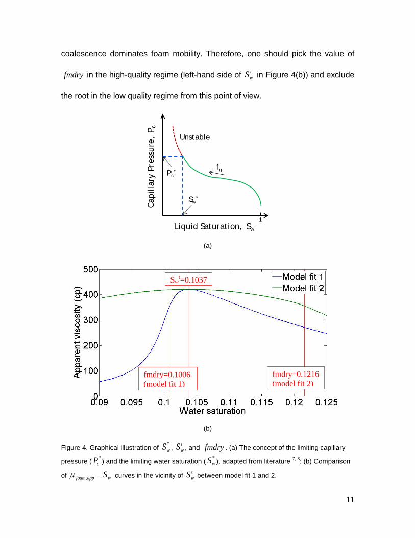
Figure 4. Graphical illustration of *wS , t

wS , and fmdry . (a) The concept of the limiting capillary

pressure ( *cP ) and the limiting water saturation ( *

wS ), adapted from literature 7, 8; (b) Comparison

of wappfoam S−,µ curves in the vicinity of twS between model fit 1 and 2.

Liquid Saturation, Sw

Cap

illar

y Pr

essu

re,

P c

Sw*

Pc*

fg

1

Unstable

Swt=0.1037

fmdry=0.1006 (model fit 1)

fmdry=0.1216 (model fit 2)

12

2.2 Discussion on multi-variable, multi-dimensional search

Multi-variable, multi-dimensional search methods are considered as useful

approaches to find an optimal set of multiple parameters. These techniques in

general fall into two categories: unconstrained methods and constrained methods.

The details of various optimization methods are available in the literature 9-12. If

the goal of fitting foam parameters is to minimize the residual sum of squares for

all available experimental data, the problem can be stated as:

∑=

−=

n

i measuredifoam

measuredifoamcalculatedifoamiepdryfmdryfmmobf

1

2

,,

,,,,),,(minµ

µµω ………...…..……(6)

..ts 0>fmmob , grwc SfmdryS −≤≤ 1 , and 0>epdry

where calculatedifoam ,,µ is the calculated foam apparent viscosity at the corresponding

gas fractional flow measuredigf ,, . The value of calculatedifoam ,,µ is computed through Eqns

(A.4) and (A.5) and the value of measuredifoam ,,µ is taken from all experimental data,

not just the transition value. A set of weighting parameters, denoted as iω in Eqn

(6), is usually employed to indicate expected standard deviation of each

experimental point. In the following analysis we hypothesize that the weighting

parameters are all equal to unity except for a value of 5 for the transition value

( 5=iω when tfoammeasuredifoam µµ =,, ).

13

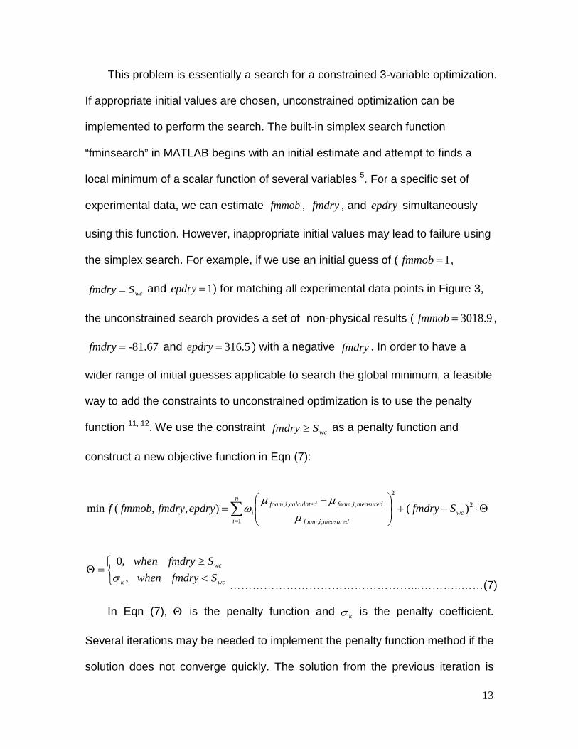
This problem is essentially a search for a constrained 3-variable optimization.

If appropriate initial values are chosen, unconstrained optimization can be

implemented to perform the search. The built-in simplex search function

“fminsearch” in MATLAB begins with an initial estimate and attempt to finds a

local minimum of a scalar function of several variables 5. For a specific set of

experimental data, we can estimate fmmob , fmdry , and epdry simultaneously

using this function. However, inappropriate initial values may lead to failure using

the simplex search. For example, if we use an initial guess of ( 1=fmmob ,

wcSfmdry = and 1=epdry ) for matching all experimental data points in Figure 3,

the unconstrained search provides a set of non-physical results ( 3018.9=fmmob ,

-81.67=fmdry and 316.5=epdry ) with a negative fmdry . In order to have a

wider range of initial guesses applicable to search the global minimum, a feasible

way to add the constraints to unconstrained optimization is to use the penalty

function 11, 12. We use the constraint wcSfmdry ≥ as a penalty function and

construct a new objective function in Eqn (7):

Θ⋅−+

−=∑

=

2

1

2

,,

,,,, )(),,(min wc

n

i measuredifoam

measuredifoamcalculatedifoami Sfmdryepdryfmdryfmmobf

µµµ

ω

<≥

=Θwck

wc

SfmdrywhenSfmdrywhen

,,0

σ …………………………………………...………..……(7)

In Eqn (7), Θ is the penalty function and kσ is the penalty coefficient.

Several iterations may be needed to implement the penalty function method if the

solution does not converge quickly. The solution from the previous iteration is

14

used as the initial guess and the penalty coefficient is increased in each iteration

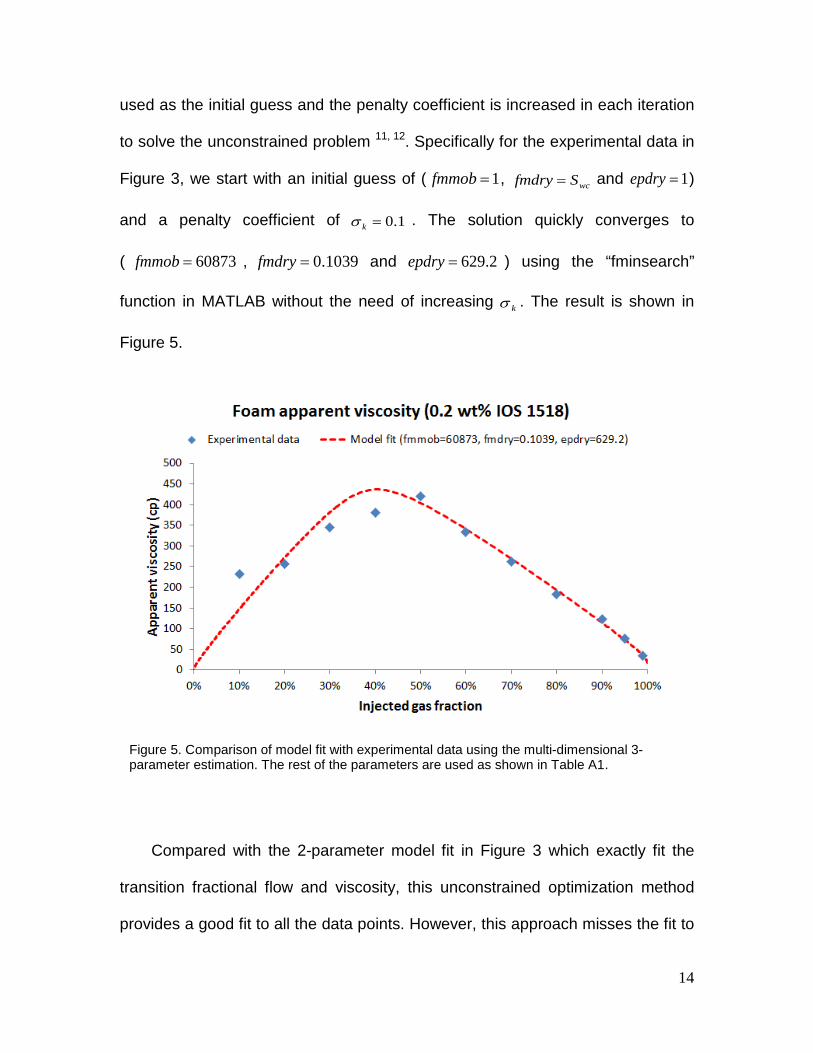
to solve the unconstrained problem 11, 12. Specifically for the experimental data in

Figure 3, we start with an initial guess of ( 1=fmmob , wcSfmdry = and 1=epdry )

and a penalty coefficient of 0.1=kσ . The solution quickly converges to

( 87306=fmmob , 0.1039=fmdry and 629.2=epdry ) using the “fminsearch”

function in MATLAB without the need of increasing kσ . The result is shown in

Figure 5.

Compared with the 2-parameter model fit in Figure 3 which exactly fit the

transition fractional flow and viscosity, this unconstrained optimization method

provides a good fit to all the data points. However, this approach misses the fit to

Figure 5. Comparison of model fit with experimental data using the multi-dimensional 3-parameter estimation. The rest of the parameters are used as shown in Table A1.

15

the transition foam quality (around 10% absolute error) as shown in Figure 5. A

closer fit to the transition data is possible by giving more weight to the transition

data during the fitting ( 5>iω when tfoammeasuredifoam µµ =,, ). The finding of

629.2=epdry indicates that a small value of epdry (less than 1000) shows a

good fit to this set of steady-state experimental data, which represents a gradual

transition between the high-quality and the low-quality foam regime. The fitting

method focusing on the transition foam data in Section 2.1 is still valuable for a

preliminary estimation of the parameters, as the strongest foam at the transition

foam quality is possibly least affected by trapped gas, minimum pressure

gradient and gravity segregation in 1-D experiments. These effects will be

evaluated in the future and added to the model fit if they significantly affect the

model fit. In general, the main challenge of using multi-variable, multi-

dimensional search is the possibility of reaching local minimum. This issue is

especially significant when available experimental data points are not abundant

and too many modeling parameters are used. To avoid this problem, one can

choose an initial guess using the 2-parameter search method shown in Section

2.1 and add constraints to the searching algorithm as needed.

2.3 Numerical oscillation in transient foam simulation

It has been noted that epdry should not be too large in order to have

acceptable stability and run time in simulators using the finite difference algorithm

6, 13. In Part 1 of this series of papers, we simulated the transient foam process of

continuous gas injection to 100% surfactant-solution-saturated porous media.

16

Now we compare the result of finite difference simulation (FD) with the method of

characteristics (MOC) and investigate how significant the numerical artifact is in

the finite difference simulation. We discuss the case with the dry-out function in

the foam model only. In order to compare the MOC solution with the FD

simulation, we use the same set of foam parameters ( 47196=fmmob ,

0.1006=fmdry and 500=epdry ) in the following computation. The rest of the

parameters are listed in Table A1.The details of the MOC calculation are shown

in the appendix. The FD algorithm with a standard IMPES (implicit in pressure

and explicit in saturation) formulation is used to simulate the transient foam

process in which 100% gas displaces 100% surfactant solution.

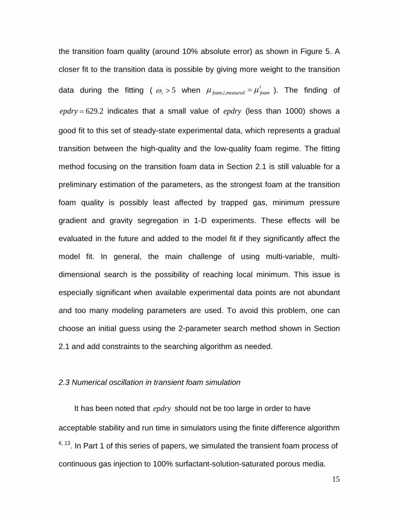
The local foam apparent viscosity ( appfoam,µ ) and the average foam apparent

viscosity ( appfoam,µ ) are defined in Eqns (8) and (9), respectively. is a

function of time and distance, which reflects the local normalized pressure

gradient as foam advances in porous media. appfoam,µ is a function of time, which

reflects the averaged, overall normalized pressure gradient in the system. The

methods for computing appfoam,µ in MOC and FD simulation are shown in the

appendix.

…………………………………………………….……….……… (8)

………………………………………….……………………..(9)

appfoam,µ

g

frg

w

rwappfoam kk

µµ

µ+

=1

,

Luuppk

gw

inoutappfoam )(

)(, +

−−=µ

17

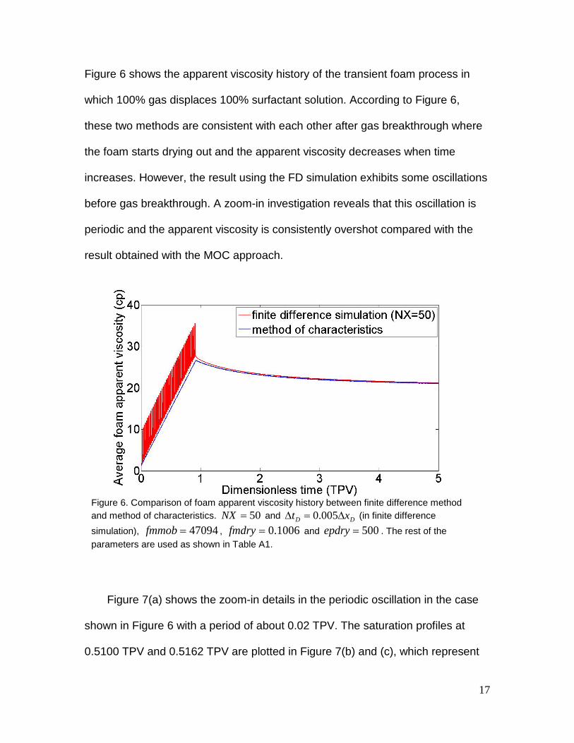
Figure 6 shows the apparent viscosity history of the transient foam process in

which 100% gas displaces 100% surfactant solution. According to Figure 6,

these two methods are consistent with each other after gas breakthrough where

the foam starts drying out and the apparent viscosity decreases when time

increases. However, the result using the FD simulation exhibits some oscillations

before gas breakthrough. A zoom-in investigation reveals that this oscillation is

periodic and the apparent viscosity is consistently overshot compared with the

result obtained with the MOC approach.

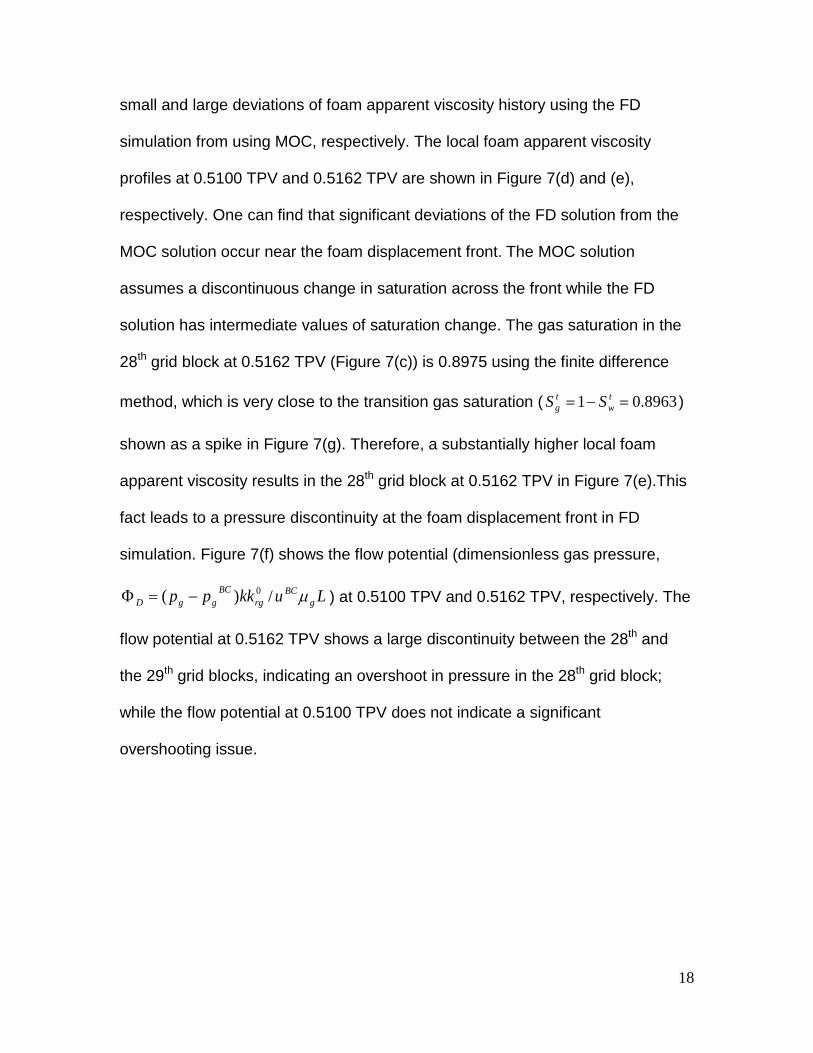
Figure 7(a) shows the zoom-in details in the periodic oscillation in the case

shown in Figure 6 with a period of about 0.02 TPV. The saturation profiles at

0.5100 TPV and 0.5162 TPV are plotted in Figure 7(b) and (c), which represent

Figure 6. Comparison of foam apparent viscosity history between finite difference method and method of characteristics. 50=NX and (in finite difference simulation), 47094=fmmob , 0.1006=fmdry and 500=epdry . The rest of the parameters are used as shown in Table A1.

DD xt ∆=∆ 0.005

18

small and large deviations of foam apparent viscosity history using the FD

simulation from using MOC, respectively. The local foam apparent viscosity

profiles at 0.5100 TPV and 0.5162 TPV are shown in Figure 7(d) and (e),

respectively. One can find that significant deviations of the FD solution from the

MOC solution occur near the foam displacement front. The MOC solution

assumes a discontinuous change in saturation across the front while the FD

solution has intermediate values of saturation change. The gas saturation in the

28th grid block at 0.5162 TPV (Figure 7(c)) is 0.8975 using the finite difference

method, which is very close to the transition gas saturation ( 0.89631 =−= tw

tg SS )

shown as a spike in Figure 7(g). Therefore, a substantially higher local foam

apparent viscosity results in the 28th grid block at 0.5162 TPV in Figure 7(e).This

fact leads to a pressure discontinuity at the foam displacement front in FD

simulation. Figure 7(f) shows the flow potential (dimensionless gas pressure,

Lukkpp gBC

rgBC

ggD µ/)( 0−=Φ ) at 0.5100 TPV and 0.5162 TPV, respectively. The

flow potential at 0.5162 TPV shows a large discontinuity between the 28th and

the 29th grid blocks, indicating an overshoot in pressure in the 28th grid block;

while the flow potential at 0.5100 TPV does not indicate a significant

overshooting issue.

19

(a) (b)

(c) (d)

(e) (f)

(g) Figure 7. Investigation of numerical oscillation in FD simulation in which 100% gas displaces surfactant solution at 100% water saturation: (a) average foam apparent viscosity history from 0.50 to 0.55 TPV; (b) saturation profile at 0.5100 TPV; (c) saturation profile at 0.5162 TPV; (d) local foam apparent viscosity profile at 0.5100 TPV; (e) local foam apparent viscosity profile at 0.5162 TPV; (f) flow potential profiles at 0.5100 TPV and 0.5162 TPV; (g) the relationship between gas saturation and foam apparent viscosity. 50=NX ,

DD xt ∆=∆ 0.005 , 47196=fmmob , 0.1006=fmdry and 500=epdry . The rest of the parameters are used as shown in Table A1.

20

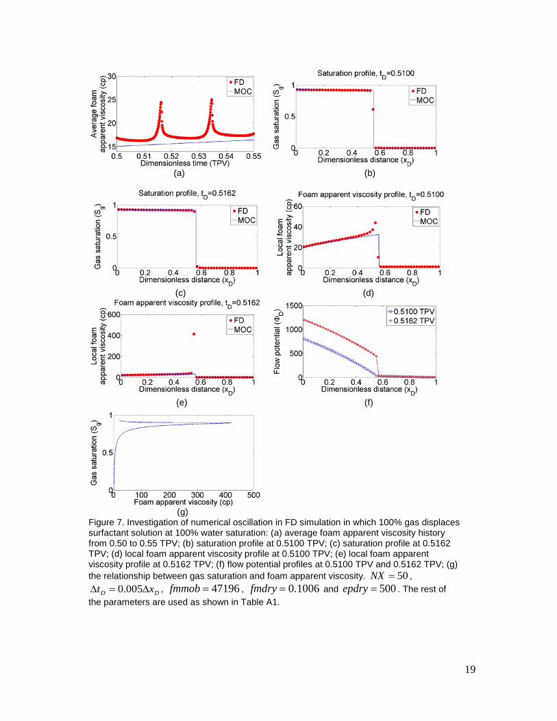
In order to understand the main factors in finite difference simulation which

contribute to this numerical artifact observed in Figure 6 and 7, we simulate five

cases of the transient foam simulation in which 100% gas displaces 100%

surfactant solution. The parameters that are altered among different cases are

shown in Table 1 in bold.

Cases 1, 2 and 3 share the same set of foam modeling parameters. The

parameter sets in all five cases in Table 1 exhibit good fit to steady-state data at

the transition foam quality ( 5.0=tgf and cpt

appfoam 421, =µ ) as shown in Figure

8(a). Figure 8(b) shows the base case (Case 1) using a total grid block numbers

of 50=NX and a time step size of DD xt ∆=∆ 0.005 , Which is essentially the same

as that in Figure 6. In Case 2 (Figure 8(c)) we decrease the time step size to 1/10

of the one in the base case, however, no significant change is observed in the

numerical oscillations. This result reveals that the IMPES simulator is numerically

Table 1. Parameters for the simulation of transient foam in Figure 8.

Parameter Case 1 Case 2 Case 3 Case 4 Case 5

DD xt ∆∆ / 0.005 0.0005 0.005 0.005 0.005

NX 50 50 200 50 50

epdry 500 500 500 500 100

fmmob 47196 47196 47196 28479 69618

fmdry 0.1006 0.1006 0.1006 0.2473 0.1020

wn 1.96 1.96 1.96 4.0 1.96

The foam modeling parameters in Table 1 are intended to fit the experimental data of 5.0=t

gf and cptappfoam 421, =µ as shown in Figure 8(a). The rest of the parameters are

used as shown in Table A1.

21

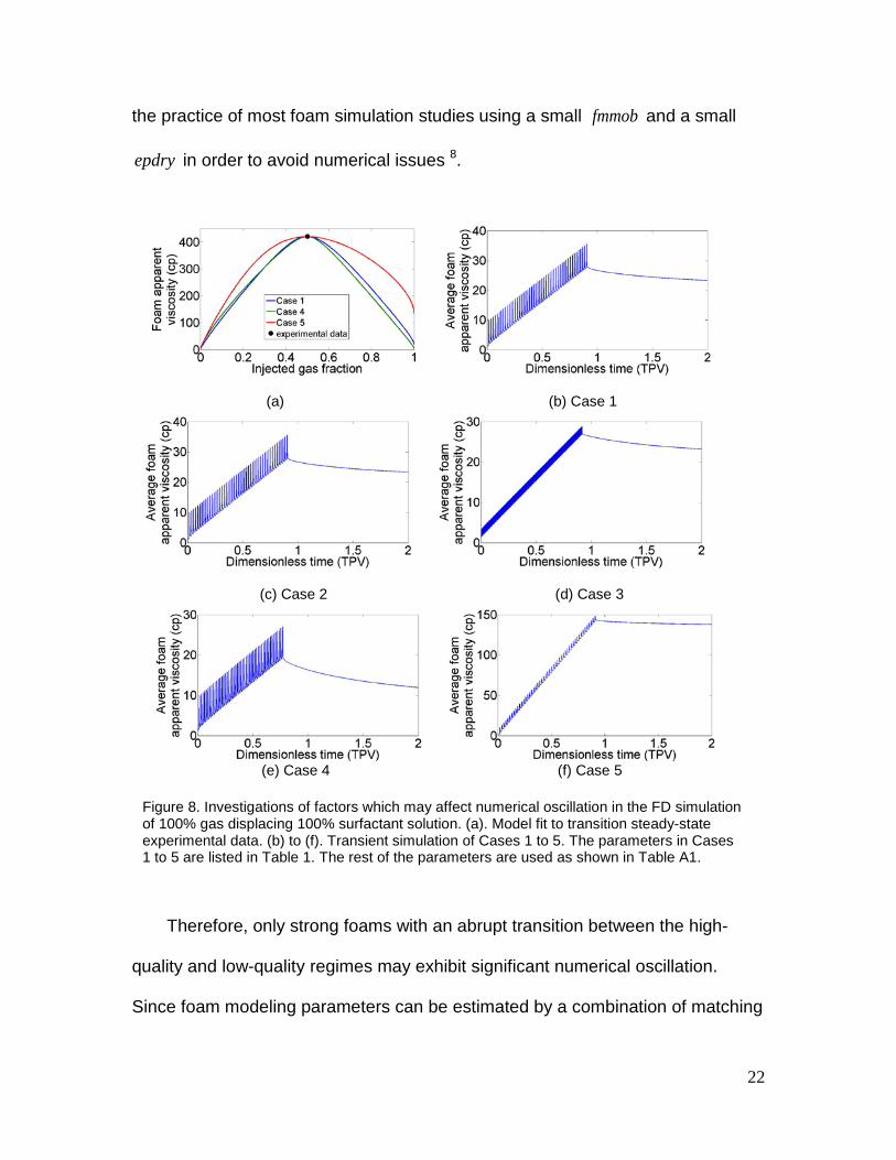
stable in terms of selection of time step size in the base case. The total grid

blocks are increased to 200=NX in Case 3 (Figure 8(d)) and significant

reduction in the amplitude of numerical oscillation is observed compared with the

base case. Also, it is observed that the frequency of the oscillation is proportional

to the number of gridblocks. This observation indicates that an increase in total

grid block numbers in the FD simulation leads to a better approximation to the

solution using the MOC approach, at the cost of increasing computational time

during the simulation. The reason behind this is that the contribution of the

pressure drop in the grid block exactly at foam displacement front is smaller

when the size of the grid block is smaller.

The parameters used in relative permeability curves and the foam modeling

parameters also affects the numerical oscillation. They can change the shape of

foam apparent viscosity as a function of saturation (Figure 7(g)), and a less sharp

peak in Figure 7(g) will result a less significant oscillation. The increase in the

exponent of the water relative permeability curve (Case 4, Figure 8(e)) from 1.96

to 4.0 does not help reduce numerical oscillation because the steady-state

appfoam,µ - gf curve in Case 4 does not differ much from that in Case 1 as shown in

Figure 8(a). As indicated in Case 5 (Figure 8(f)), a decrease in epdry causes a

decrease in the amplitude of numerical oscillation in foam apparent viscosity

history before gas breakthrough. This result indicates that a more gradual

transition between the high-quality and low-quality regimes reduces numerical

oscillation. Additionally, a weaker foam, which requires a smaller fmmob , can

also lead to a smaller amplitude in numerical oscillation. This is consistent with

22

the practice of most foam simulation studies using a small fmmob and a small

epdry in order to avoid numerical issues 8.

Therefore, only strong foams with an abrupt transition between the high-

quality and low-quality regimes may exhibit significant numerical oscillation.

Since foam modeling parameters can be estimated by a combination of matching

(a) (b) Case 1

(c) Case 2 (d) Case 3

(e) Case 4 (f) Case 5

Figure 8. Investigations of factors which may affect numerical oscillation in the FD simulation of 100% gas displacing 100% surfactant solution. (a). Model fit to transition steady-state experimental data. (b) to (f). Transient simulation of Cases 1 to 5. The parameters in Cases 1 to 5 are listed in Table 1. The rest of the parameters are used as shown in Table A1.

23

both steady-state and transient experiments, a practical way to minimize this

numerical oscillation issue is to select an acceptable number of total grid blocks

and a large time step which does not affect the numerical stability in the FD

simulation. The crux to reduce the numerical oscillation in foam apparent

viscosity history is to smear out the foam displacement front and to avoid the

sharp change in local apparent viscosity at the foam front in the FD simulation.

For applications such as co-injecting gas and surfactant solution into the system

which has not been previously filled with surfactant solution, the local apparent

viscosity at the foam front is control by both water saturation and surfactant

concentration if one uses the dry-out function and the surfactant-concentration-

dependent function simultaneously in the foam model. If a dispersive surfactant

front exists at the foam front (assuming no chromatographic retardation), a

weaker foam front can result compared with the full-strength foam at the foam

bank, leading to lower amplitude in numerical oscillation (data not shown).

2.4 Sensitivity of foam parameters

Parameters in the STARSTM foam model are sensitive to the estimation of

the parameters which are used to model gas-water flow in porous media in the

absence of foam. It was found that in general rwk functions were more nonlinear

for consolidated sandstones than for sandpacks and that an increase in the

nonlinearity of rwk could benefit the Surfactant-Alternating-Gas (SAG) process 14.

It is important to recognize that one cannot apply the same set of foam

parameters to different porous media without experimental verification. For

24

example, the transition foam quality ( tgf ) was shown to decrease significantly

when permeability decreased from a sandpack to a Berea core using the same

surfactant formulation (Bio-Terge AS-40 surfactant supplied by Stepan, a C14-16

sodium alpha-olefin sulfonate) 15. In order to demonstrate the sensitivity of foam

modeling parameters with respect to two-phase flow parameters, we match the

experimental data ( 5.0)( =measuredf tg and cpmeasuredt

appfoam 421)(, =µ ) using the

dry-out function in the STARSTM foam model with changes in the parameters of

the exponent in the rwk function ( wn ) and connate water saturation ( wcS ) shown in

Figure 9 and 10.

The nonlinearity of the rwk function is controlled by the exponent wn as

shown in Figure 9(a). An increase in wn leads to a more curved rwk curve. It is

found that the experimental data ( 5.0)( =measuredf tg and

cpmeasuredtappfoam 421)(, =µ ) in Figure 9(b) cannot be fit with the STARSTM foam

model if wn is equal to 1. We fit the experimental data at the transition foam

quality using values of wn from 1.5 to 4.0. The model fit appears similar in the

low-quality regime and distinguishable differences in the high-quality-regime with

higher predicted apparent viscosity using lower value of wn . Moreover, Figure 9(c)

and (d) show strong dependence of the foam modeling parameters fmmob and

fmdry on the exponent wn of the rwk curve with a preset epdry of 500. fmmob

decreases by about one-half when wn increases from 1.5 to 4.0, while fmdry

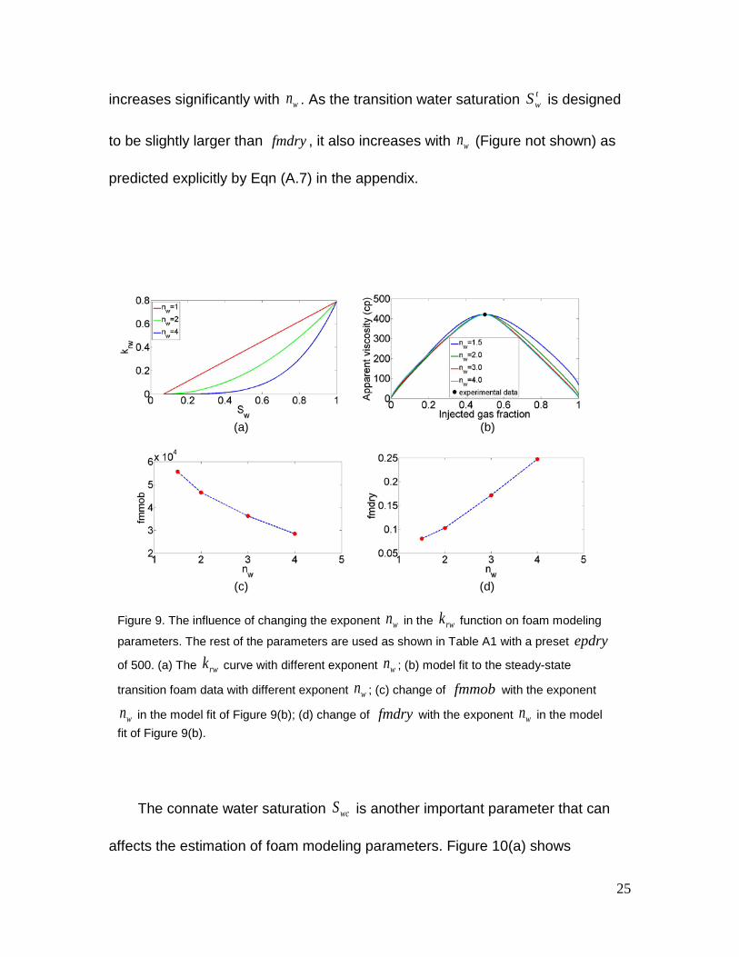
25

increases significantly with wn . As the transition water saturation twS is designed

to be slightly larger than fmdry , it also increases with wn (Figure not shown) as

predicted explicitly by Eqn (A.7) in the appendix.

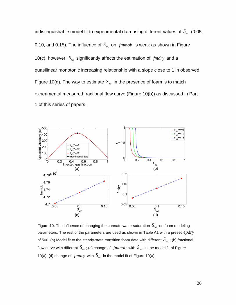
The connate water saturation wcS is another important parameter that can

affects the estimation of foam modeling parameters. Figure 10(a) shows

(a) (b)

(c) (d)

Figure 9. The influence of changing the exponent wn in the rwk function on foam modeling

parameters. The rest of the parameters are used as shown in Table A1 with a preset epdry of 500. (a) The rwk curve with different exponent wn ; (b) model fit to the steady-state

transition foam data with different exponent wn ; (c) change of fmmob with the exponent

wn in the model fit of Figure 9(b); (d) change of fmdry with the exponent wn in the model fit of Figure 9(b).

26

indistinguishable model fit to experimental data using different values of wcS (0.05,

0.10, and 0.15). The influence of wcS on fmmob is weak as shown in Figure

10(c), however, wcS significantly affects the estimation of fmdry and a

quasilinear monotonic increasing relationship with a slope close to 1 in observed

Figure 10(d). The way to estimate wcS in the presence of foam is to match

experimental measured fractional flow curve (Figure 10(b)) as discussed in Part

1 of this series of papers.

(a) (b)

(c) (d)

Figure 10. The influence of changing the connate water saturation wcS on foam modeling

parameters. The rest of the parameters are used as shown in Table A1 with a preset epdry of 500. (a) Model fit to the steady-state transition foam data with different wcS ; (b) fractional

flow curve with different wcS ; (c) change of fmmob with wcS in the model fit of Figure

10(a); (d) change of fmdry with wcS in the model fit of Figure 10(a).

27

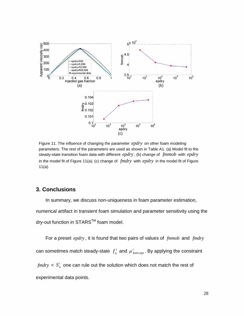
In Part 1 of this series of papers we showed a wide range of epdry could be

used to estimate fmmob and fmdry at the transition foam quality in steady-state

experiments. We verify the results here in Figure 11 with the numerical method

proposed in Figure 1 and show the parameter sensitivity to epdry . Figure 11(a)

showed that different preset epdry ranging from 500 to 500,000 can fit the

transition experimental data using the non-graphical approach proposed in

Figure 1. fmmob decreases when epdry increases (Figure 11(b)) till fmmob

approaches a plateau value, while fmdry only exhibits a subtle change in the

third significant digit in response to epdry (Figure 11(c)). This is because fmdry

asymptotically approaches twS when epdry is sufficiently large, while t

wS is

independent of epdry according to Eqn (A.7) in the appendix. In the case of

5.0=tgf and cpt

appfoam 421, =µ , twS is 0.1037 calculated through Eqn (A.7).

28

3. Conclusions

In summary, we discuss non-uniqueness in foam parameter estimation,

numerical artifact in transient foam simulation and parameter sensitivity using the

dry-out function in STARSTM foam model.

For a preset epdry , it is found that two pairs of values of fmmob and fmdry

can sometimes match steady-state tgf and t

appfoam,µ . By applying the constraint

fmdry < twS one can rule out the solution which does not match the rest of

experimental data points.

(a) (b)

(c)

Figure 11. The influence of changing the parameter epdry on other foam modeling parameters. The rest of the parameters are used as shown in Table A1. (a) Model fit to the steady-state transition foam data with different epdry ; (b) change of fmmob with epdry in the model fit of Figure 11(a); (c) change of fmdry with epdry in the model fit of Figure 11(a).

29

To match all available data points using multi-dimensional, multi-variable

search, one can use the unconstrained optimization approach with an

appropriate initial guess which is close to the global optimum. The penalty

function method for constrained optimization can be applied for a wider range of

initial guesses.

Finite difference simulation for the transient foam process is generally

consistent with the method of characteristics. A less abrupt change in foam

mobility in the foam displacement front is needed to minimize the oscillation

numerical artifact in the average foam apparent viscosity history. Small epdry

leads to lower amplitude in numerical oscillation and larger apparent viscosity

when foam breaks through.

Foam parameters are sensitive to the parameters in relatively permeability

curves. For foam parameter estimation by matching steady-state tgf and t

appfoam,µ ,

the water relative permeability exponent wn affects the estimation of both fmmob

and fmdry , and the connate water saturation wcS is particularly influential in

estimating fmdry . An increase in epdry causes a decrease in fmmob , but no

substantial change is found in fmdry .

4. Nomenclature

epdry = a parameter regulating the slope of 2F curve near fmdry

f = fractional flow

30

tgf = transition foam quality where the maximum foam apparent viscosity is

achieved

FM = a dimensionless foam function in STARSTM foam model

fmdry = critical water saturation in STARSTM foam model

fmmob = reference mobility reduction factor in STARSTM foam model

k = permeability, darcy

rk = relative permeability

0rwk = end-point relative permeability of aqueous phase

0rgk = end-point relative permeability of gaseous phase

L = length of the porous medium, ft

p = pressure, psi

cP = capillary pressure, psi

*cP = limiting capillary pressure, psi

u = superficial (Darcy) velocity, dayft /

S = saturation

twS = transition water saturation where the maximum foam apparent viscosity is

achieved

t = time, s

µ = viscosity, cp

= local foam apparent viscosity, cp appfoam,µ

31

= average foam apparent viscosity, cp

tappfoam,µ = maximum foam apparent viscosity obtained at the transition foam

quality, cp

φ = porosity

DΦ = flow potential (dimensionless gas pressure)

ω = weighting parameter in multi-variable, multi-dimensional search

Θ = penalty function in multi-variable, multi-dimensional search

σ = penalty coefficient in multi-variable, multi-dimensional search

Superscripts

BC = boundary condition

nf = without foam

f = with foam

gn = exponent in rgk curve

wn = exponent in rwk curve

t = transition between high-quality and low-quality foam

Subscripts

D = dimensionless

g = gaseous phase

gr = residual gas

appfoam,µ

32

w = aqueous phase

wc = connate water

5. Appendix

The technique to model 1-D incompressible isothermal foam flow through

porous media using the dry-out function involves 11 parameters ( wcS , grS , 0rwk ,

wn , 0rgk , gn , wµ , gµ , fmmob , fmdry , and epdry ) as shown in Eqns (A.1) to (A.5).

1=+ gw SS ……………………………………………..…………………………...…(A.1)

wn

wcgr

wcwrwrw SS

SSkk )1

(0

−−−

×= ……………………………………………..…………...…(A.2)

−

+×+×

−−−

−×=×=

π)](arctan[5.01

1)1

1(0

fmdrySepdryfmmobSSSSkFMkk

w

n

wcgr

wcwrg

nfrg

frg

g

……………..…………………………..………………..……………..……………...(A.3)

)()(1

1

gf

rg

g

w

wrwg

SkSk

f µµ

⋅+= ………………………….……….…………..…………...…(A.4)

g

gf

rg

w

wrwappfoam SkSk

µµ

µ)()(

1,

+= ……………………………………………..…..………(A.5)

In this work we mainly investigate the estimation of the three foam parameters

33

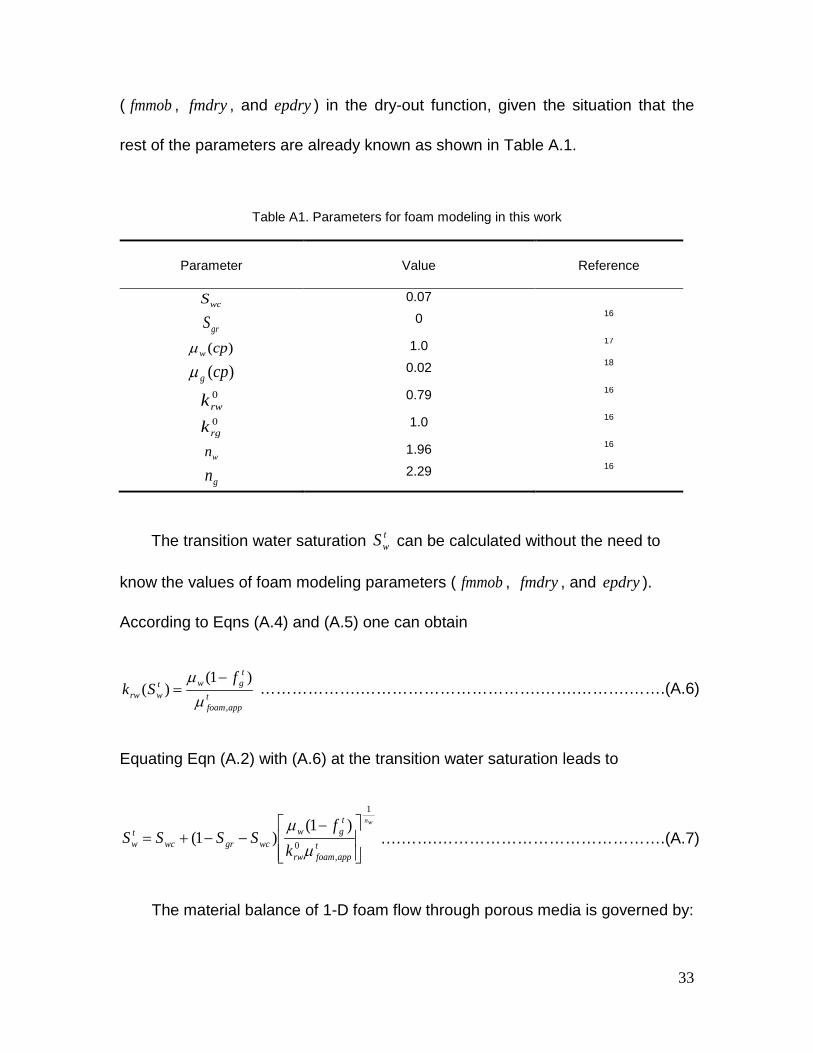
( fmmob , fmdry , and epdry ) in the dry-out function, given the situation that the

rest of the parameters are already known as shown in Table A.1.

Table A1. Parameters for foam modeling in this work

Parameter Value Reference

wcS 0.07

grS 0 16

)(cpwµ 1.0 17

)(cpgµ 0.02 18

0rwk

0.79 16

0rgk

1.0 16

wn 1.96 16

gn 2.29 16

The transition water saturation twS can be calculated without the need to

know the values of foam modeling parameters ( fmmob , fmdry , and epdry ).

According to Eqns (A.4) and (A.5) one can obtain

tappfoam

tgwt

wrw

fSk

,

)1()(

µµ −

= ……………….…………………………….…….……….…….(A.6)

Equating Eqn (A.2) with (A.6) at the transition water saturation leads to

wn

tappfoamrw

tgw

wcgrwctw k

fSSSS

1

,0

)1()1(

−−−+=

µµ

….…….…………………………………….(A.7)

The material balance of 1-D foam flow through porous media is governed by:

34

0=∂∂

+∂∂

xu

tS wwφ ………………………………………………………...…...………..(A.8)

0=∂

∂+

∂

∂

xu

tS ggφ …………………………………………………………...…...……..(A.9)

If the dimensionless variables L

tutBC

D φ= ,

LxxD = , BC

ww u

uf = , BCg

g uu

f = are used,

we can get the following partial differential equation for the gas phase:

0=∂

∂+

∂

∂

D

g

D

g

xf

tS

……………………………………………..…………….…………...(A.10)

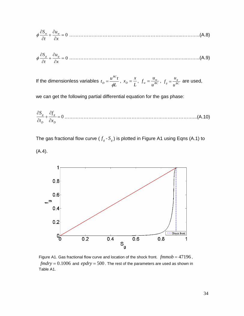
The gas fractional flow curve ( gf - gS ) is plotted in Figure A1 using Eqns (A.1) to

(A.4).

Figure A1. Gas fractional flow curve and location of the shock front. 47196=fmmob , 0.1006=fmdry and 500=epdry . The rest of the parameters are used as shown in

Table A1.

35

As shown in Figure A1, a shock front will result if 100% gas displaces 100%

surfactant solution. The shock saturation is determined by drawing a straight line

from the initial condition ( ICgS , = 0) which is tangential to the fractional flow curve.

In the case in Figure A1 we get shockgS , = 0.9182. Then wave velocities and

saturation profiles can be constructed based on Figure A1 using Eqn (A.11):

aSg

g

aSD

D

ggdSdf

dtdx

==

= ………………………………………..………………………..(A.11)

If the saturation “a” in Eqn (A.11) is smaller than shockgS , , then the wave velocity at

aSg = is equal to the shock velocity.

According the definitions of the local foam apparent viscosity (Eqn (8)) and

the average foam apparent viscosity (Eqn(9)), the relationship is shown in Eqn

(A.12):

………………………………………….…… (A.12)

∫

∫

∫

∫

=

+

=

⋅

⋅−⋅−

−=

⋅+

−=

+−

−=

1

0 ,

1

0

0

0

,

1

1

1

)()(

Dappfoam

D

g

frg

w

rw

L

g

frg

w

rw

L

gw

gw

inoutappfoam

dx

dxkk

dxdxdp

dxdpkk

dxdpkkL

k

dxdxdp

uuLk

Luuppk

µ

µµ

µµ

µ

36

Note that at a specific time = both and are functions of , while

the saturation profile is already known by computing the wave velocities. Thus

Eqn (A.12) can be approximated by numerical integration using available data

points:

………..…...………..… (A.13)

Eqn (A.13) is used to calculate the average foam apparent viscosity in the MOC

solution. For FD simulation, the average foam apparent viscosity is approximated

by the pressure difference between the first and the last grid blocks (Eqn (A.14)):

………………………………………...…………(A.14)

6. Acknowledgment

We acknowledge financial support from the Abu Dhabi National Oil

Company (ADNOC), the Abu Dhabi Oil R&D Sub-Committee, Abu Dhabi

Company for Onshore Oil Operations (ADCO), Zakum Development Company

(ZADCO), Abu Dhabi Marine Operating Company (ADMA-OPCO) and the

Petroleum Institute (PI), U.A.E and partial support from the US Department of

Energy (under Award No. DE-FE0005902), Petróleos Mexicanos (PEMEX) and

Shell Global Solutions International.

Dt 0t rwk frgk gS

∑∫=

∆

+

≈

+

=n

iiD

g

igf

rg

w

igrwD

g

frg

w

rwappfoam x

SkSkdx

kk 1,

,,

1

0, )()(11

µµµµ

µ

1)()( 1

, −⋅

+−

−=NX

NXLuu

ppk

gw

NXappfoamµ

37

We thank Yongchao Zeng at Rice University for assistance in development

of the MATLAB code.

7. References

1. Computer Modeling Group, STARSTM user's guide. Calgary, Alberta, Canada 2007. 2. Farajzadeh, R.; Wassing, B. M.; Boerrigter, P. M., Foam assisted gas-oil gravity drainage in naturally-fractured reservoirs. J. Pet. Sci. Eng. 2012, 94-95, 112-122. 3. Ma, K.; Lopez-Salinas, J. L.; Puerto, M. C.; Miller, C. A.; Biswal, S. L.; Hirasaki, G. J., Estimation of parameters for the simulation of foam flow through porous media: Part 1; the dry-out effect. Energy Fuels, Submitted. 4. Lopez-Salinas, J. L.; Ma, K.; Puerto, M. C.; Miller, C. A.; Biswal, S. L.; Hirasaki, G. J., Estimation of parameters for the simulation of foam flow through porous media: Part 2; effects of surfactant concentration and fluid velocity. In preparation. 5. The MathWorks Inc, MATLAB User's Guide. Natick, MA, USA 2012. 6. Cheng, L.; Reme, A. B.; Shan, D.; Coombe, D. A.; Rossen, W. R., Simulating foam processes at high and low foam qualities. In SPE/DOE Improved Oil Recovery Symposium (SPE 59287), Tulsa, Oklahoma, 2000. 7. Khatib, Z. I.; Hirasaki, G. J.; Falls, A. H., Effects of capillary pressure on coalescence and phase mobilities in foams flowing through porous media. SPE Reservoir Eng. 1988, 3, (3), 919-926. 8. Farajzadeh, R.; Andrianov, A.; Krastev, R.; Hirasaki, G. J.; Rossen, W. R., Foam-oil interaction in porous media: Implications for foam assisted enhanced oil recovery. Adv. Colloid Interface Sci. 2012, 183, 1-13. 9. Aster, R. C.; Thurber, C. H.; Borchers, B., Parameter estimation and inverse problems. Elsevier Academic Press: Amsterdam ; Boston, 2005; p xii, 301 p. 10. Fletcher, R., Practical methods of optimization. 2nd ed.; Wiley: Chichester ; New York, 1987; p 436 p. 11. Avriel, M., Nonlinear programming : analysis and methods. Prentice-Hall: Englewood Cliffs, 1976; p xv, 512 p. 12. Bazaraa, M. S.; Sherali, H. D.; Shetty, C. M., Nonlinear programming : theory and algorithms. 3rd ed.; Wiley: New York, NY ; Chichester, 2006; p xv, 853 p. 13. Zanganeh, M. N.; Kraaijevanger, J. F. B. M.; Buurman, H. W.; Jansen, J. D.; Rossen, W. R., Adjoint-Based Optimization of a Foam EOR Process. In 13th European Conference on the Mathematics of Oil Recovery, Biarritz, France, 2012. 14. Ashoori, E.; Rossen, W. R., Can Formation Relative Permeabilities Rule Out a Foam EOR Process? SPE J. 2012, 17, (2), 340-351. 15. Alvarez, J. M.; Rivas, H. J.; Rossen, W. R., Unified model for steady-state foam behavior at high and low foam qualities. SPE J. 2001, 6, (3), 325-333.

38

16. Kam, S. I.; Nguyen, Q. P.; Li, Q.; Rossen, W. R., Dynamic simulations with an improved model for foam generation. SPE J. 2007, 12, (1), 35-48. 17. Bruges, E. A.; Latto, B.; Ray, A. K., New correlations and tables of coefficient of viscosity of water and steam up to 1000 bar and 1000 degrees C. Int. J. Heat Mass Transfer 1966, 9, (5), 465-480. 18. Lemmon, E. W.; Jacobsen, R. T., Viscosity and thermal conductivity equations for nitrogen, oxygen, argon, and air. Int. J. Thermophys. 2004, 25, (1), 21-69.