Estimation of Internal Pit depth Growth and Reliability of Aged Oil and Gas Pipelines - A Monte

Carlo simulation Approach.

Chinedu I. Ossai*, Brian Boswell, Ian J. Davies

Department of Mechanical Engineering, Curtin University, GPO Box U1987, Perth, WA 6845,

Australia.

Abstract

To estimate the internal pit depth growth and reliability of aged oil and gas pipelines, a Monte Carlo

simulation approach was adopted. The average maximum pit depths of corroded pipelines were

correlated with the operating parameters - temperature, CO2 partial pressure, pH, flow rate, sulphate

ion concentration, chloride ion concentration, water cut and wall shear stress via a multivariate

regression analysis. Poisson Square Wave Model (PSWM) was used to predict the time lapse of the pit

depth growth using the statistical best fit of the maximum pit depth and operating parameters as

boundary conditions. Weibull probability function was used to determine the failure intensity and

survivability of the pipelines for different distribution types whereas inspection data from a Magnetic

Flux Leakage (MFL) in-line-inspected transmission pipeline were used to test the application of the

model. The future pit depth distribution, survivability and failure rate of this transmission pipeline

were also determined with the result showing that the model is vital for future internal pit depth

growth and reliability estimation from single field inspection data.

Keywords: Pit depth; Internal corrosion; Aged pipeline; Reliability; Survival probability

1.0 Introduction

Corrosion estimate is fundamental to the health monitoring of pipelines 1 since there is a tendency of

pipelines decreasing in reliability with increase in age of operation especially when there is corrosion

defect2, 3. This is because as the corrosion wastage of the pipelines increase, the residual strength

reduces due to the reducing pipe-wall thickness4, 5 hence, increasing the likelihood of failure over time.

Corrosion can also result in unscheduled downtime especially for pitting corrosion, crevice corrosion,

stress corrosion cracking and fatigue corrosion since they occur without outward signs on the

facilities6. Reliability is a measure of the ability of an asset to perform its intended function within a

stipulated time frame. The reliability of a pipeline is dependent on the corrosion wastage over time

hence, corrosion probability distribution is a vital tool for developing reliability and risk-based

inspection models 2. Since future pit depth distribution can be estimated from previous pit depth

distribution using Monte Carlo simulation (due to its ability to generate future data based on random

walk principles 7, 8), it therefore follows that, proper application of Monte Carlo simulation technique

is necessary for estimating the reliability of ageing pipelines.

C. I. Ossai, B. Boswell and I. J. Davies, “Estimation of internal pit depth growth and reliability of aged oil and gaspipelines - A Monte Carlo simulation approach”, Corrosion (ISSN 0010-9312), in press (accepted May 6th 2015)

Page 2 of 30

Corrosion growth models are vital for the development of pipeline integrity management programs,

which can include inspection, mitigation and repair activities 9, 10, 11, 12. Hence, time-dependent

reliability of corroded high pressure offshore pipelines were establish by researchers 13 who utilized

homogenous gamma process based corrosion growth model to determine the expected future

corrosion wastage of the pipelines. These authors used the internal pressure, which was modelled

with Poison Square Wave Model (PSWM) to calculate the corrosion growth rate and established the

time of pipeline failure with respect to small leaks, large leaks and ruptures 13. Again, the knowledge

of pit depth transition probability was used by some researchers to develop a reliability model for

managing pitting corrosion of oil and gas pipelines 14. This model will make it possible to design a

mitigation program, which will enhance pipeline lifecycle through maintenance, inspection and

repairs. Similarly, the use of historic data for calculating the reliability of corroded non-piggable

upstream pipelines exposed to corrosion by statistical analyses was done by Valor et al. 15 who

determined the corrosion distribution trend of the pit depths and correlated them to the failure

pressure at a future time.

Different researcher have shown that pit depth growth process of pipelines is a time-dependent

stochastic damage process that has exponential 16,17, logarithmic 16, lognormal 17,18, gamma 19, Weibull

19, normal 16,17 and generalized extreme value 20 growth patterns however, long time exposure of pit

depths have been shown to follow Fretchet distribution 2,21, 22. Furthermore, pit depth growth can be

determined using limited data via extreme value analysis, which depends on the maximum pit depth

at an exposure time for extrapolating future pit depth distribution over a long time exposure 23.

Researchers such as Mohd and Paik 17 investigated the relationship between internal pit depth growth

and age of offshore pipelines statistically and showed the correlation between age of pipelines and

Weibull scale and shape parameters. Although the work did not show the reliability of these pipelines

at various ages, it is a good outlook for the progression of pit depth with time. Other researchers that

have been pertinent about pit depth growth includes Alamilla and Sosa 8 that used mathematical

modelling to describe the propagation of cracks resulting from pitting corrosion defects. The authors

showed that probability density function and propagation function of the pit depths are vital for

characterizing the evolution of pit depth with time. Chookah et al. 24 on the other hand utilized

probabilistic physics-of-failure based mechanistic model to predict the growth trend of cracks on a

pipeline associated with pitting corrosion. This work considered the amplitude and frequency of the

mechanical stress initiated by the internal pressure and chemical corrosive species inside the pipeline

in estimating the fatigue crack growth. The authors used a Monte Carlo simulation approach, which

incorporated the experimental findings of the physical parameters - applied stress, frequency and the

concentration of the corrosive chemical agents as a function of the corrosion current in the modelling

Page 3 of 30

and subsequently in calculating the reliability of the pipelines. Soares and Garbatov 7 on their part used

a non-linear corrosion model based on exponential corrosion wastage to determine the reliability of a

plate by quantifying the collapse strength against the compressive loading in the presence of

corrosion. Hu et al. 25 also predicted pipeline reliability using Monte Carlo simulation approach by

determining the crack growth with time as a function of operating pressure, corrosion electric current

and pipe wall thickness. Again, Bazan and Beck 18 used Poisson Square Wave Model (PSWM) to

determine the proportionality constant of pitting corrosion defect in a bid to establish a continuous

growth of the corrosion defect with time. The authors concluded that a random linear growth model

determined with PSWM conservatively predicted the long run corrosion growth of the selected field

data but may not be optimal for the inspection intervals. Other authors such as Zhang and Zhou 26

incorporated a second order polynomial dynamic linear model with Bayesian updating in a Monte

Carlo simulation in order to estimate corrosion defect growth whereas Hasan et al. 27 calculated failure

probability of pipelines by characterizing corrosion defect based on geometry of the longitudinal

section of the corrosion, growth rate and remaining mechanical hoop strength capacity.

The aim of this research is to complement the works reviewed above by determining the statistical

characteristics of field data comprising of maximum pit depths and operating parameters –

temperature, flow rate, pH, CO2 partial pressure, sulphate ion concentration, chloride ion

concentration, water cut and wall shear stress of onshore pipelines in a bid to establish the

relationship between them whilst investing the internal maximum pit depth growth of the pipelines

over time using Monte Carlo simulation. The maximum pit depths of the pipelines were classified as

low, moderate, high and severe whereas the time lapse for pit depth growth was determined using

PSWM, which estimated pitting time based on independent arrival rate of a Homogenous Poisson

Process (HPP). The statistical best fit of the maximum pit depth and operating parameters were used

as input for the Monte Carlo simulation whereas the reliability of the pipeline as time elapsed were

calculated using Weibull probability based on different distributions - Gamma, lognormal,

exponential, generalized extreme value, Weibull and extreme value. A Magnetic Flux Leakage (MFL)

in-line-inspection (ILI) data of an API X52 pipeline were used to test the proposed model.

The limitation of this research is the inability to consider the impacts of H2S and O2 in the pitting

corrosion of the studied pipelines. This is because the H2S concentrations of the studied fields are very

small and hence will not enhance the pitting corrosion of the studied pipelines, which were

predominantly under the influence of sweet corrosion. Seeing that H2S concentration is minimal and

the corrosion mechanism was dominated by sweet corrosion, it was not necessary to consider the

effect of O2 in the pitting process because O2 have been shown to significantly enhance pitting

corrosion in the presence of H2S 28. Furthermore, research has shown that at limited concentration of

Page 4 of 30

H2S, O2 generally have small impact on the corrosion rates of carbon steel 29 whereas H2S results in

pitting corrosion when the concentration is more than 100ppm30.

2.0 Experimental Procedure

2.1 Field Data Acquisition

Internal pitting corrosion data of pipelines used for transmission of multiphase fluid from oil fields in

Niger Delta region of Nigeria and the operating parameters of the pipelines – temperature, pH, CO2

partial pressure, production rate, sulphate ion concentration, chloride ion concentration, water cut

and operating pressure were obtained from the company’s database. A total of six hundred sampled

data of the maximum pit depths of the pipelines measured over a period of ten years were used for

this study. The maximum pit depths were determined using pulse-echo Ultrasonic thickness

Measurement (UTM) technique whereas the operating parameters were measured as part of the

routine quality assurance procedure in the organization. The linear flow rate of the fluid and the wall

shear stress were determined using the production rate and operating pressures inside the pipelines

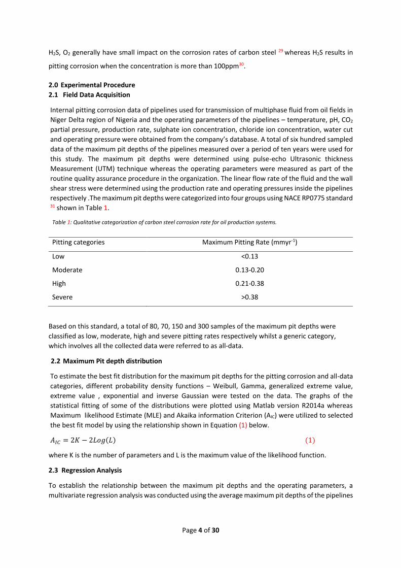
respectively .The maximum pit depths were categorized into four groups using NACE RP0775 standard 31 shown in Table 1.

Table 1: Qualitative categorization of carbon steel corrosion rate for oil production systems.

Pitting categories Maximum Pitting Rate (mmyr-1)

Low <0.13

Moderate 0.13-0.20

High 0.21-0.38

Severe >0.38

Based on this standard, a total of 80, 70, 150 and 300 samples of the maximum pit depths were

classified as low, moderate, high and severe pitting rates respectively whilst a generic category,

which involves all the collected data were referred to as all-data.

2.2 Maximum Pit depth distribution

To estimate the best fit distribution for the maximum pit depths for the pitting corrosion and all-data

categories, different probability density functions – Weibull, Gamma, generalized extreme value,

extreme value , exponential and inverse Gaussian were tested on the data. The graphs of the

statistical fitting of some of the distributions were plotted using Matlab version R2014a whereas

Maximum likelihood Estimate (MLE) and Akaika information Criterion (AIC) were utilized to selected

the best fit model by using the relationship shown in Equation (1) below.

𝐴𝐼𝐶 = 2𝐾 − 2𝐿𝑜𝑔(𝐿) (1)

where K is the number of parameters and L is the maximum value of the likelihood function.

2.3 Regression Analysis

To establish the relationship between the maximum pit depths and the operating parameters, a

multivariate regression analysis was conducted using the average maximum pit depths of the pipelines

Page 5 of 30

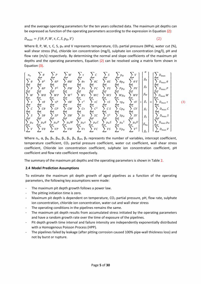
and the average operating parameters for the ten years collected data. The maximum pit depths can

be expressed as function of the operating parameters according to the expression in Equation (2):

𝐷𝑚𝑎𝑥 = 𝑓(𝜃, 𝑃,𝑊, 𝜏, 𝐶, 𝑆, 𝑝𝐻 , 𝑉) (2)

Where θ, P, W, τ, C, S, pH and V represents temperature, CO2 partial pressure (MPa), water cut (%),

wall shear stress (Pa), chloride ion concentration (mg/l), sulphate ion concentration (mg/l), pH and

flow rate (m/s) respectively. By determining the normal and slope coefficients of the maximum pit

depths and the operating parameters, Equation (2) can be resolved using a matrix form shown in

Equation (3).

[ 𝑛𝑣 ∑𝜃 ∑𝑃 ∑𝑊 ∑𝜏 ∑𝐶 ∑𝑆 ∑𝑝𝐻 ∑𝑉

∑𝜃 ∑𝜃2 ∑𝜃𝑃 ∑𝜃𝑊 ∑𝜃𝜏 ∑𝜃𝐶 ∑𝜃𝑆 ∑𝜃𝑝𝐻 ∑𝜃 𝑉

∑𝑃 ∑𝜃𝑃 ∑𝑃2 ∑𝑃𝑊 ∑𝑃𝜏 ∑𝑃𝐶 ∑𝑃𝑆 ∑𝑃𝑝𝐻 ∑𝑃𝑉

∑𝑊 ∑𝑊𝜃 ∑𝑊𝑃 ∑𝑊2 ∑𝑊𝜏 ∑𝑊𝐶 ∑𝑊𝑆 ∑𝑊𝑝𝐻 ∑𝑊𝑉

∑𝜏 ∑𝜏𝜃 ∑𝜏𝑃 ∑𝜏𝑊 ∑𝜏2 ∑𝜏𝐶 ∑𝜏𝑆 ∑𝜏𝑝𝐻 ∑𝜏𝑉

∑𝐶 ∑𝐶𝜃 ∑𝐶𝑃 ∑𝐶𝑊 ∑𝐶𝜏 ∑𝐶2 ∑𝐶 𝑆 ∑𝐶𝑝𝐻 ∑𝐶𝑉

∑𝑆 ∑𝑆𝜃 ∑𝑆𝑃 ∑𝑆𝑊 ∑𝑆𝜏 ∑𝑆𝐶 ∑𝑆2 ∑𝑆𝑝𝐻 ∑𝑆𝑉

∑𝑝𝐻 ∑𝑝𝐻𝜃 ∑𝑝𝐻𝑃 ∑𝑝𝐻𝑊 ∑𝑝𝐻𝜏 ∑𝑝𝐻𝐶 ∑𝑝𝐻𝑆 ∑𝑝𝐻2 ∑𝑝𝐻𝑉

∑𝑉 ∑𝑉𝜃 ∑𝑉𝑃 ∑𝑉𝑊 ∑𝑉𝜏 ∑𝑉𝐶 ∑𝑉𝑆 ∑𝑉𝑝𝐻 ∑𝑉2]

∗

[

𝛼

𝛽𝜃

𝛽𝑃

𝛽𝑊

𝛽𝜏

𝛽𝐶

𝛽𝑆

𝛽𝑝𝐻

𝛽𝑉 ]

=

[ ∑𝐷max

∑𝐷𝑚𝑎𝑥 𝜃

∑𝐷𝑚𝑎𝑥 𝑃

∑𝐷𝑚𝑎𝑥 𝑊

∑𝐷𝑚𝑎𝑥 𝜏

∑𝐷𝑚𝑎𝑥 𝐶

∑𝐷𝑚𝑎𝑥 𝑆

∑𝐷𝑚𝑎𝑥 𝑝𝐻

∑𝐷𝑚𝑎𝑥 𝑉 ]

(3)

Where nv, α, βθ, βP, βW, βτ, βC, βS, βpH, βV represents the number of variables, intercept coefficient,

temperature coefficient, CO2 partial pressure coefficient, water cut coefficient, wall shear stress

coefficient, Chloride ion concentration coefficient, sulphate ion concentration coefficient, pH

coefficient and flow rate coefficient respectively.

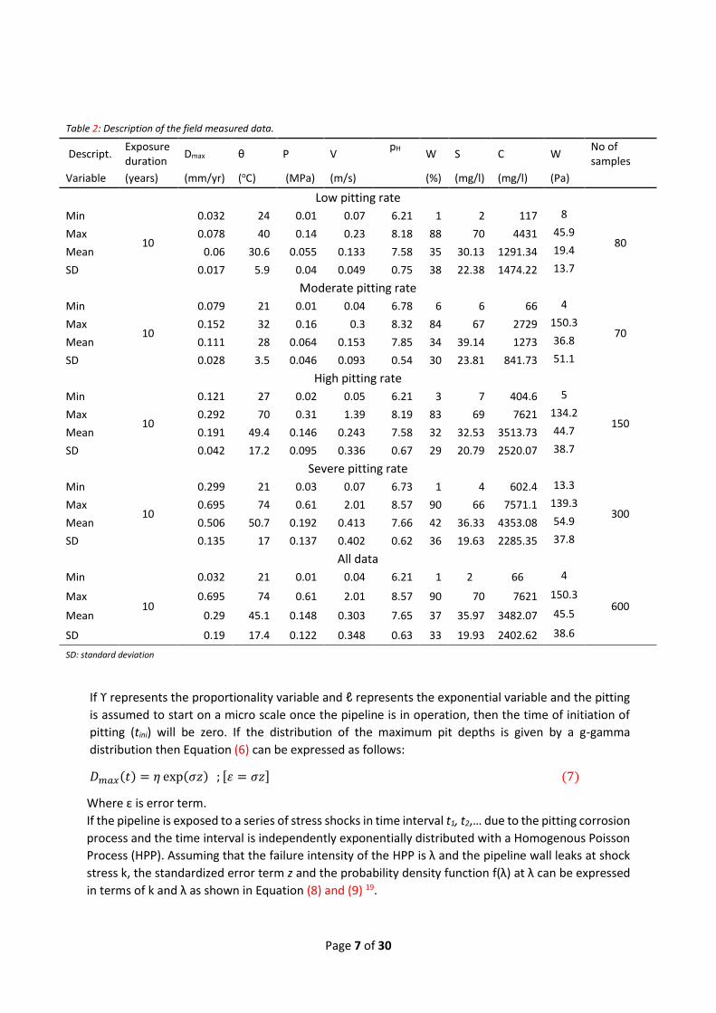
The summary of the maximum pit depths and the operating parameters is shown in Table 2.

2.4 Model Prediction Assumptions

To estimate the maximum pit depth growth of aged pipelines as a function of the operating

parameters, the following key assumptions were made:

- The maximum pit depth growth follows a power law.

- The pitting initiation time is zero.

- Maximum pit depth is dependent on temperature, CO2 partial pressure, pH, flow rate, sulphate

ion concentration, chloride ion concentration, water cut and wall shear stress

- The operating conditions in the pipelines remains the same.

- The maximum pit depth results from accumulated stress initiated by the operating parameters

and have a random growth rate over the time of exposure of the pipelines.

- Pit depth growth time interval and failure intensity are independently exponentially distributed

with a Homogenous Poisson Process (HPP).

- The pipelines failed by leakage (after pitting corrosion caused 100% pipe-wall thickness loss) and

not by burst or rupture.

Page 6 of 30

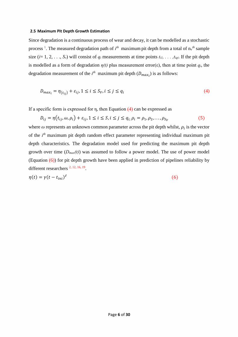
2.5 Maximum Pit Depth Growth Estimation

Since degradation is a continuous process of wear and decay, it can be modelled as a stochastic

process 1. The measured degradation path of ith maximum pit depth from a total of nvth sample

size (i= 1, 2, . . ., Sv) will consist of qi measurements at time points ti1, . . . ,tiqi. If the pit depth

is modelled as a form of degradation η(t) plus measurement error(ε), then at time point qi, the

degradation measurement of the ith maximum pit depth (𝐷𝑚𝑎𝑥𝑖) is as follows:

𝐷𝑚𝑎𝑥𝑖= 𝜂(𝑡𝑖𝑗)

+ 𝜀𝑖𝑗 , 1 ≤ 𝑖 ≤ 𝑆𝑉, 𝑖 ≤ 𝑗 ≤ 𝑞𝑖 (4)

If a specific form is expressed for η, then Equation (4) can be expressed as

𝐷𝑖𝑗 = 𝜂(𝑡𝑖𝑗, 𝜔, 𝜌𝑖) + 𝜀𝑖𝑗 , 1 ≤ 𝑖 ≤ 𝑆, 𝑖 ≤ 𝑗 ≤ 𝑞𝑖; 𝜌𝑖 = 𝜌1, 𝜌2, . . . , 𝜌𝑆𝑉 (5)

where ω represents an unknown common parameter across the pit depth whilst, 𝜌𝑖 is the vector

of the ith maximum pit depth random effect parameter representing individual maximum pit

depth characteristics. The degradation model used for predicting the maximum pit depth

growth over time (Dmax(t)) was assumed to follow a power model. The use of power model

(Equation (6)) for pit depth growth have been applied in prediction of pipelines reliability by

different researchers 2, 12, 16, 19.

𝜂(𝑡) = 𝛾(𝑡 − 𝑡𝑖𝑛𝑖)ℓ (6)

Page 7 of 30

If ϒ represents the proportionality variable and ℓ represents the exponential variable and the pitting

is assumed to start on a micro scale once the pipeline is in operation, then the time of initiation of

pitting (tini) will be zero. If the distribution of the maximum pit depths is given by a g-gamma

distribution then Equation (6) can be expressed as follows:

𝐷𝑚𝑎𝑥(𝑡) = 𝜂 exp(𝜎𝑧) ; [𝜀 = 𝜎𝑧] (7)

Where ε is error term.

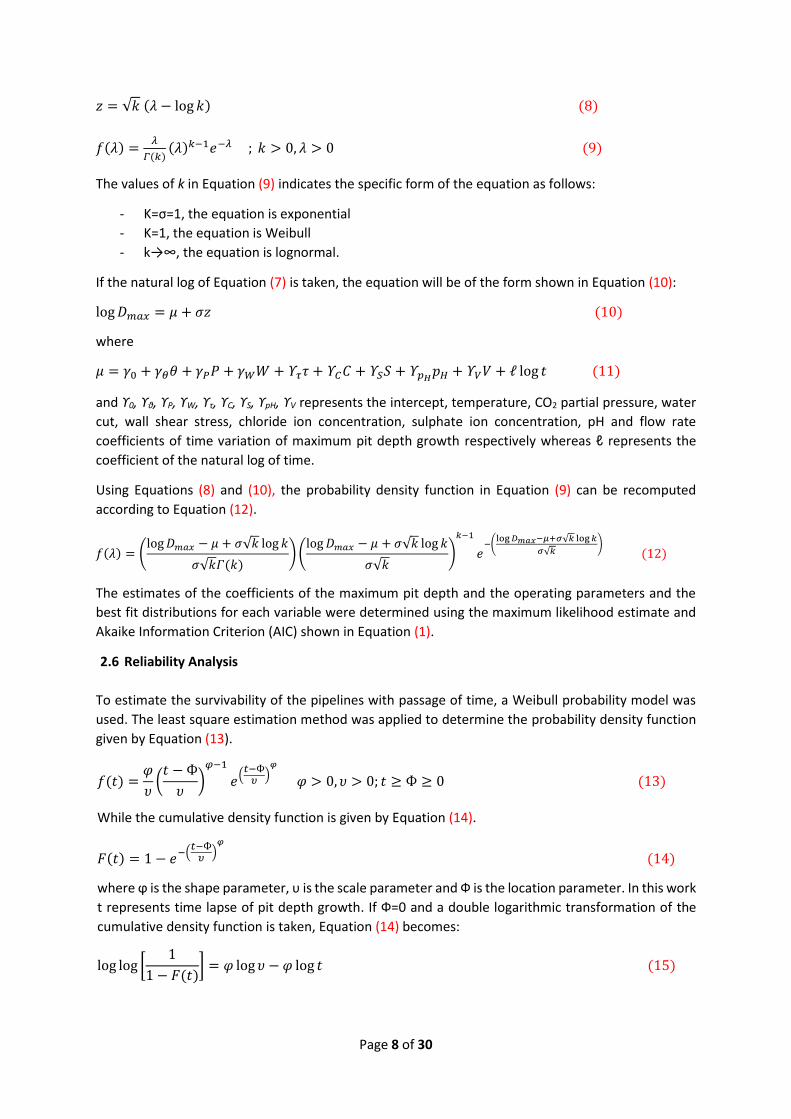
If the pipeline is exposed to a series of stress shocks in time interval t1, t2,… due to the pitting corrosion

process and the time interval is independently exponentially distributed with a Homogenous Poisson

Process (HPP). Assuming that the failure intensity of the HPP is λ and the pipeline wall leaks at shock

stress k, the standardized error term z and the probability density function f(λ) at λ can be expressed

in terms of k and λ as shown in Equation (8) and (9) 19.

Table 2: Description of the field measured data.

Descript. Exposure duration

Dmax θ P V pH

W S C W No of samples

Variable (years) (mm/yr) (oC) (MPa) (m/s) (%) (mg/l) (mg/l) (Pa)

Low pitting rate

Min

10

0.032 24 0.01 0.07 6.21 1 2 117 8

80 Max 0.078 40 0.14 0.23 8.18 88 70 4431 45.9

Mean 0.06 30.6 0.055 0.133 7.58 35 30.13 1291.34 19.4

SD 0.017 5.9 0.04 0.049 0.75 38 22.38 1474.22 13.7

Moderate pitting rate

Min

10

0.079 21 0.01 0.04 6.78 6 6 66 4

70 Max 0.152 32 0.16 0.3 8.32 84 67 2729 150.3

Mean 0.111 28 0.064 0.153 7.85 34 39.14 1273 36.8

SD 0.028 3.5 0.046 0.093 0.54 30 23.81 841.73 51.1

High pitting rate

Min

10

0.121 27 0.02 0.05 6.21 3 7 404.6 5

150 Max 0.292 70 0.31 1.39 8.19 83 69 7621 134.2

Mean 0.191 49.4 0.146 0.243 7.58 32 32.53 3513.73 44.7

SD 0.042 17.2 0.095 0.336 0.67 29 20.79 2520.07 38.7

Severe pitting rate

Min

10

0.299 21 0.03 0.07 6.73 1 4 602.4 13.3

300 Max 0.695 74 0.61 2.01 8.57 90 66 7571.1 139.3

Mean 0.506 50.7 0.192 0.413 7.66 42 36.33 4353.08 54.9

SD 0.135 17 0.137 0.402 0.62 36 19.63 2285.35 37.8

All data

Min

10

0.032 21 0.01 0.04 6.21 1 2 66 4

600 Max 0.695 74 0.61 2.01 8.57 90 70 7621 150.3

Mean 0.29 45.1 0.148 0.303 7.65 37 35.97 3482.07 45.5

SD 0.19 17.4 0.122 0.348 0.63 33 19.93 2402.62 38.6

SD: standard deviation

Page 8 of 30

𝑧 = √𝑘 (𝜆 − log 𝑘) (8)

𝑓(𝜆) =𝜆

𝛤(𝑘)(𝜆)𝑘−1𝑒−𝜆 ; 𝑘 > 0, 𝜆 > 0 (9)

The values of k in Equation (9) indicates the specific form of the equation as follows:

- K=σ=1, the equation is exponential

- K=1, the equation is Weibull

- k→∞, the equation is lognormal.

If the natural log of Equation (7) is taken, the equation will be of the form shown in Equation (10):

log𝐷𝑚𝑎𝑥 = 𝜇 + 𝜎𝑧 (10)

where

𝜇 = 𝛾0 + 𝛾𝜃𝜃 + 𝛾𝑃𝑃 + 𝛾𝑊𝑊 + ϒ𝜏𝜏 + ϒ𝐶𝐶 + ϒ𝑆𝑆 + ϒ𝑝𝐻𝑝𝐻 + ϒ𝑉𝑉 + ℓ log 𝑡 (11)

and ϒ0, ϒθ, ϒP, ϒW, ϒτ, ϒC, ϒS, ϒpH, ϒV represents the intercept, temperature, CO2 partial pressure, water

cut, wall shear stress, chloride ion concentration, sulphate ion concentration, pH and flow rate

coefficients of time variation of maximum pit depth growth respectively whereas ℓ represents the

coefficient of the natural log of time.

Using Equations (8) and (10), the probability density function in Equation (9) can be recomputed

according to Equation (12).

𝑓(𝜆) = (log𝐷𝑚𝑎𝑥 − 𝜇 + 𝜎√𝑘 log 𝑘

𝜎√𝑘𝛤(𝑘))(

log𝐷𝑚𝑎𝑥 − 𝜇 + 𝜎√𝑘 log 𝑘

𝜎√𝑘)

𝑘−1

𝑒−(

log𝐷𝑚𝑎𝑥−𝜇+𝜎√𝑘 log𝑘

𝜎√𝑘) (12)

The estimates of the coefficients of the maximum pit depth and the operating parameters and the

best fit distributions for each variable were determined using the maximum likelihood estimate and

Akaike Information Criterion (AIC) shown in Equation (1).

2.6 Reliability Analysis

To estimate the survivability of the pipelines with passage of time, a Weibull probability model was

used. The least square estimation method was applied to determine the probability density function

given by Equation (13).

𝑓(𝑡) =𝜑

𝜐(𝑡 − Ф

𝜐)𝜑−1

𝑒(𝑡−Ф𝜐

)𝜑

𝜑 > 0, 𝜐 > 0; 𝑡 ≥ Ф ≥ 0 (13)

While the cumulative density function is given by Equation (14).

𝐹(𝑡) = 1 − 𝑒−(

𝑡−Ф𝜐

)𝜑

(14)

where ϕ is the shape parameter, υ is the scale parameter and Ф is the location parameter. In this work

t represents time lapse of pit depth growth. If Ф=0 and a double logarithmic transformation of the

cumulative density function is taken, Equation (14) becomes:

log log [1

1 − 𝐹(𝑡)] = 𝜑 log 𝜐 − 𝜑 log 𝑡 (15)

Page 9 of 30

In order to apply least square method for estimating the scale and shape parameters, the pipeline

time of pitting failure will be ranked with Equation (16).

𝑀𝑅 =𝑖 − 0.3

𝑚 + 0.4 (16)

Where MR is the median rank; m is the number of observed failures; i is ranked time lapse for pit depth

growth of the pipeline.

Since Equation (15) is linear, the following relationship can be deduced:

�̅� =1

𝑚∑log [log (

1

1 − 𝑀𝑅)]

𝑛

𝑖=1

(17)

�̅� =1

𝑚∑log 𝑡𝑖 (18)

𝑚

𝑖=1

𝜑 ={𝑚∑ (log 𝑡𝑖)

𝑚𝑖=1 ∗ log(log𝑀𝑅)} − {∑ log[log𝑀𝑅]𝑚

𝑖=1 ∗ [∑ log 𝑡𝑖𝑚𝑖=1 ]}

{𝑚 ∑ (log 𝑡𝑖)2𝑚

𝑖=1 − (∑ (log 𝑡𝑖)𝑚𝑖=1 )

2}

(19)

𝜐 = 𝑒(�̅� −

�̅�𝜑)

(20)

The failure intensity can be calculated using the shape and scale parameters as shown in Equation

(21):

𝜆(𝑡) =𝜑

𝜐(𝑡

𝜐)𝜑−1

, 𝑡 > 0 (21 )

The survivor function (R (t)) is given as follows:

𝑅(𝑡) = 𝑒−(𝜐𝑡)𝜑 ( 22)

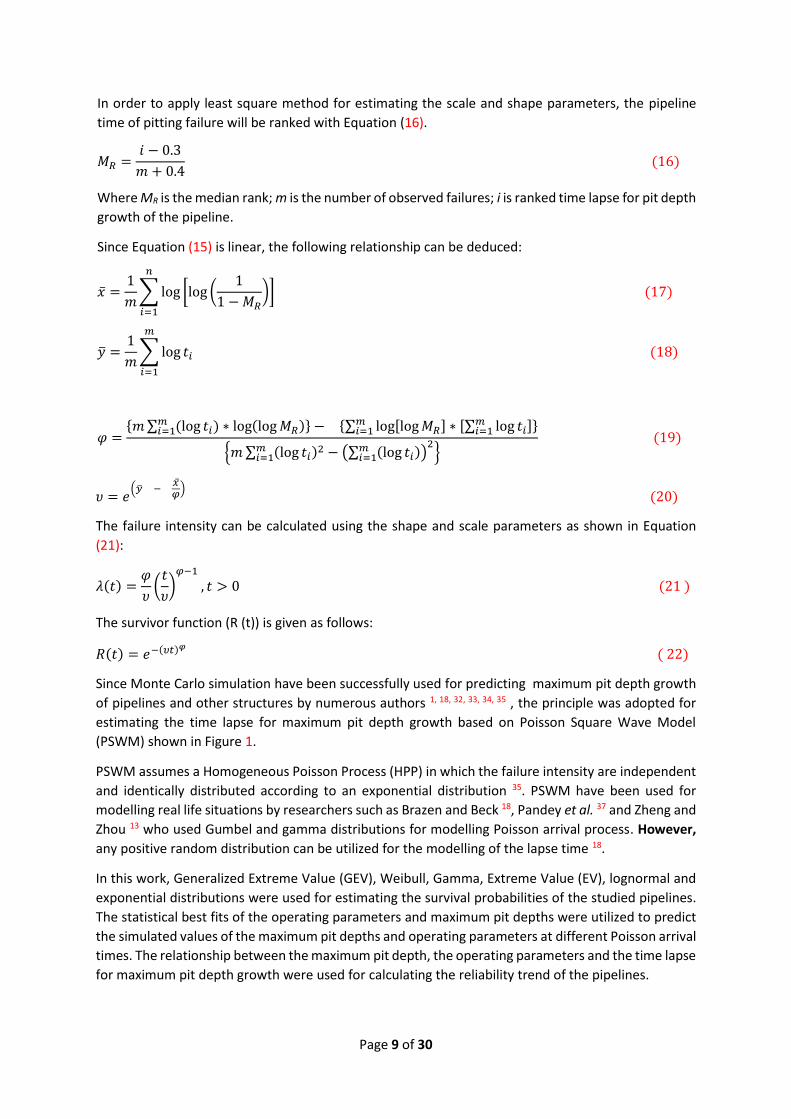
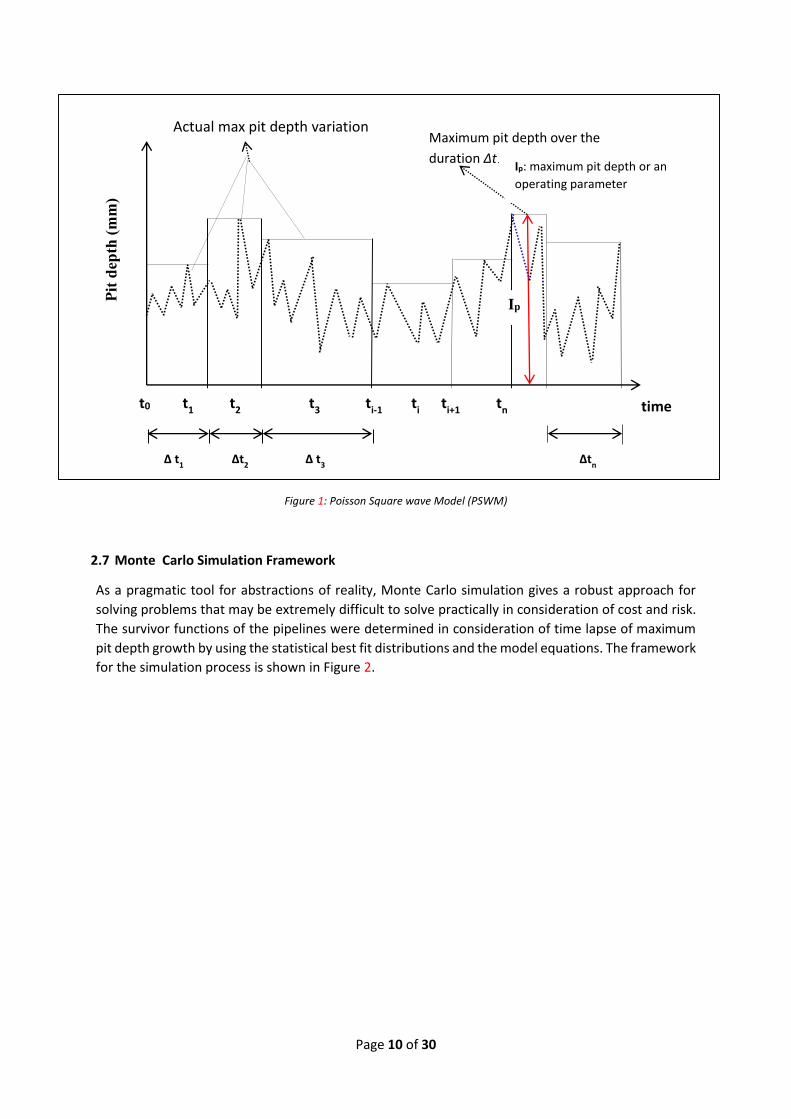
Since Monte Carlo simulation have been successfully used for predicting maximum pit depth growth

of pipelines and other structures by numerous authors 1, 18, 32, 33, 34, 35 , the principle was adopted for

estimating the time lapse for maximum pit depth growth based on Poisson Square Wave Model

(PSWM) shown in Figure 1.

PSWM assumes a Homogeneous Poisson Process (HPP) in which the failure intensity are independent

and identically distributed according to an exponential distribution 35. PSWM have been used for

modelling real life situations by researchers such as Brazen and Beck 18, Pandey et al. 37 and Zheng and

Zhou 13 who used Gumbel and gamma distributions for modelling Poisson arrival process. However,

any positive random distribution can be utilized for the modelling of the lapse time 18.

In this work, Generalized Extreme Value (GEV), Weibull, Gamma, Extreme Value (EV), lognormal and

exponential distributions were used for estimating the survival probabilities of the studied pipelines.

The statistical best fits of the operating parameters and maximum pit depths were utilized to predict

the simulated values of the maximum pit depths and operating parameters at different Poisson arrival

times. The relationship between the maximum pit depth, the operating parameters and the time lapse

for maximum pit depth growth were used for calculating the reliability trend of the pipelines.

Page 10 of 30

Figure 1: Poisson Square wave Model (PSWM)

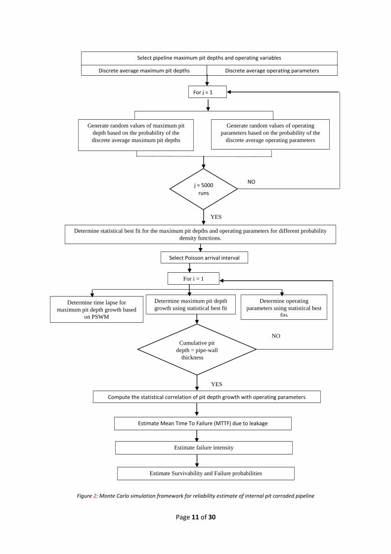
2.7 Monte Carlo Simulation Framework

As a pragmatic tool for abstractions of reality, Monte Carlo simulation gives a robust approach for

solving problems that may be extremely difficult to solve practically in consideration of cost and risk.

The survivor functions of the pipelines were determined in consideration of time lapse of maximum

pit depth growth by using the statistical best fit distributions and the model equations. The framework

for the simulation process is shown in Figure 2.

Ip

t0 t1 t2 t3 ti-1 ti ti+1 tn

∆ t1 ∆t

2 ∆ t

3 ∆t

n

Maximum pit depth over the

duration ∆ti

Actual max pit depth variation

time

Ip: maximum pit depth or an

operating parameter

Pit

dep

th (

mm

)

Page 11 of 30

Figure 2: Monte Carlo simulation framework for reliability estimate of internal pit corroded pipeline

Discrete average maximum pit depths Discrete average operating parameters

Select pipeline maximum pit depths and operating variables

For j = 1

Generate random values of maximum pit

depth based on the probability of the

discrete average maximum pit depths

Generate random values of operating

parameters based on the probability of the

discrete average operating parameters

j = 5000

runs

Carlo

NO

YES

Determine statistical best fit for the maximum pit depths and operating parameters for different probability

density functions.

Select Poisson arrival interval

For i = 1

Determine time lapse for

maximum pit depth growth based

on PSWM

Determine maximum pit depth

growth using statistical best fit Determine operating

parameters using statistical best

fits

Cumulative pit

depth = pipe-wall

thickness = n

NO

YES

Compute the statistical correlation of pit depth growth with operating parameters

Estimate Mean Time To Failure (MTTF) due to leakage

Estimate Survivability and Failure probabilities

Estimate failure intensity

Page 12 of 30

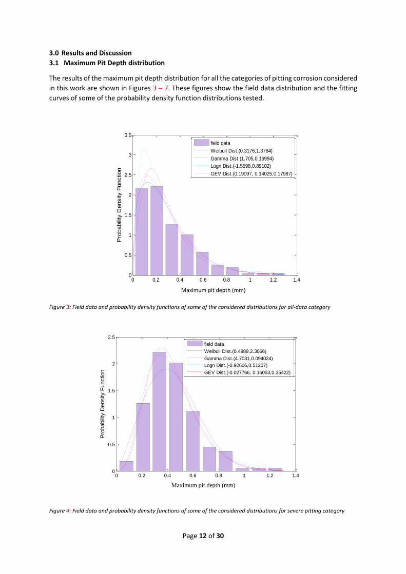
3.0 Results and Discussion

3.1 Maximum Pit Depth distribution

The results of the maximum pit depth distribution for all the categories of pitting corrosion considered

in this work are shown in Figures 3 – 7. These figures show the field data distribution and the fitting

curves of some of the probability density function distributions tested.

Figure 3: Field data and probability density functions of some of the considered distributions for all-data category

Figure 4: Field data and probability density functions of some of the considered distributions for severe pitting category

0 0.2 0.4 0.6 0.8 1 1.2 1.40

0.5

1

1.5

2

2.5

3

3.5

Maximum Pit Depth(mm/yr)

Pro

babili

ty D

ensity F

unction

field data

Weibull Dist.(0.3176,1.3784)

Gamma Dist.(1.705,0.16994)

Logn Dist.(-1.5598,0.89102)

GEV Dist.(0.19097, 0.14025,0.17987)

Maximum pit depth (mm)

0 0.2 0.4 0.6 0.8 1 1.2 1.40

0.5

1

1.5

2

2.5

Maximum Pit Depth(mm/yr)

Pro

babili

ty D

ensity

Functio

n

field data

Weibull Dist.(0.4989,2.3066)

Gamma Dist.(4.7031,0.094024)

Logn Dist.(-0.92606,0.51207)

GEV Dist.(-0.027766, 0.16053,0.35422)

Maximum pit depth (mm)

Page 13 of 30

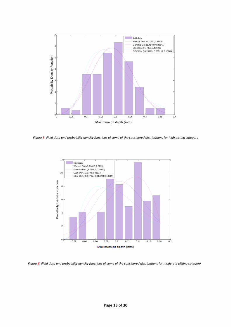
Figure 5: Field data and probability density functions of some of the considered distributions for high pitting category

Figure 6: Field data and probability density functions of some of the considered distributions for moderate pitting category

0 0.05 0.1 0.15 0.2 0.25 0.3 0.35 0.40

1

2

3

4

5

6

7

Maximum Pit Depth(mm/yr)

Pro

bab

ility

Den

sity F

un

ctio

n

field data

Weibull Dist.(0.21223,3.1845)

Gamma Dist.(6.4548,0.029541)

Logn Dist.(-1.7366,0.45923)

GEV Dist.(-0.26119, 0.065117,0.16705)

Maximum pit depth (mm)

0 0.02 0.04 0.06 0.08 0.1 0.12 0.14 0.16 0.18 0.20

2

4

6

8

10

12

Maximum Pit Depth(mm/yr)

Pro

bab

ility

Den

sity F

un

ctio

n

field data

Weibull Dist.(0.12413,2.7219)

Gamma Dist.(3.7748,0.029473)

Logn Dist.(-2.3342,0.63323)

GEV Dist.(-0.57792, 0.048593,0.10219)

Page 14 of 30

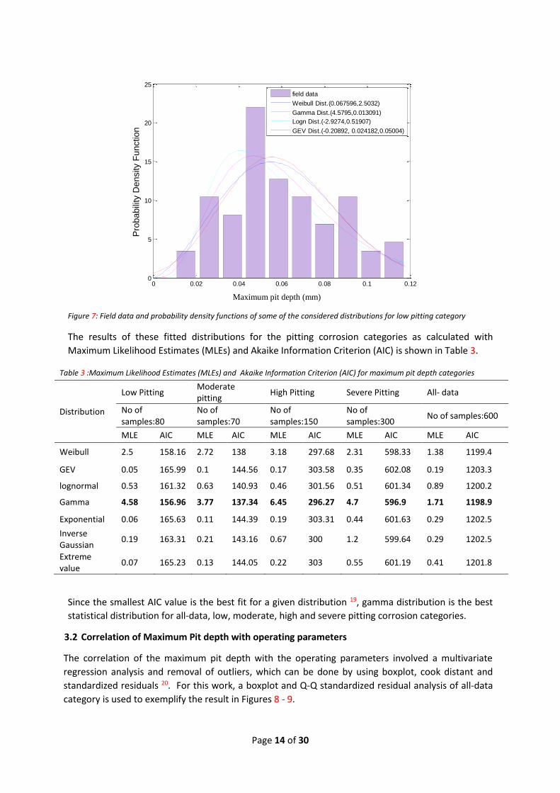
Figure 7: Field data and probability density functions of some of the considered distributions for low pitting category

The results of these fitted distributions for the pitting corrosion categories as calculated with

Maximum Likelihood Estimates (MLEs) and Akaike Information Criterion (AIC) is shown in Table 3.

Table 3 :Maximum Likelihood Estimates (MLEs) and Akaike Information Criterion (AIC) for maximum pit depth categories

Distribution

Low Pitting Moderate pitting

High Pitting Severe Pitting All- data

No of samples:80

No of samples:70

No of samples:150

No of samples:300

No of samples:600

MLE AIC MLE AIC MLE AIC MLE AIC MLE AIC

Weibull 2.5 158.16 2.72 138 3.18 297.68 2.31 598.33 1.38 1199.4

GEV 0.05 165.99 0.1 144.56 0.17 303.58 0.35 602.08 0.19 1203.3

lognormal 0.53 161.32 0.63 140.93 0.46 301.56 0.51 601.34 0.89 1200.2

Gamma 4.58 156.96 3.77 137.34 6.45 296.27 4.7 596.9 1.71 1198.9

Exponential 0.06 165.63 0.11 144.39 0.19 303.31 0.44 601.63 0.29 1202.5

Inverse Gaussian

0.19 163.31 0.21 143.16 0.67 300 1.2 599.64 0.29 1202.5

Extreme value

0.07 165.23 0.13 144.05 0.22 303 0.55 601.19 0.41 1201.8

Since the smallest AIC value is the best fit for a given distribution 19, gamma distribution is the best

statistical distribution for all-data, low, moderate, high and severe pitting corrosion categories.

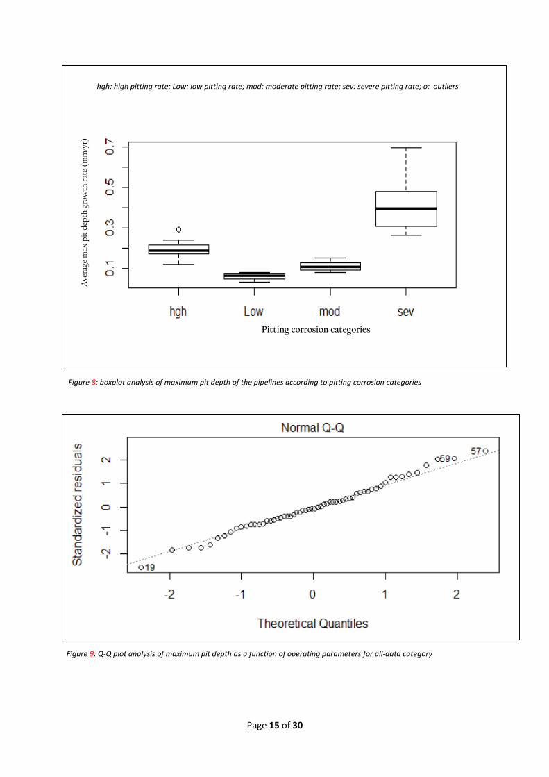
3.2 Correlation of Maximum Pit depth with operating parameters

The correlation of the maximum pit depth with the operating parameters involved a multivariate

regression analysis and removal of outliers, which can be done by using boxplot, cook distant and

standardized residuals 20. For this work, a boxplot and Q-Q standardized residual analysis of all-data

category is used to exemplify the result in Figures 8 - 9.

0 0.02 0.04 0.06 0.08 0.1 0.120

5

10

15

20

25

Maximum Pit Depth(mm/yr)

Pro

babili

ty D

ensity F

unction

field data

Weibull Dist.(0.067596,2.5032)

Gamma Dist.(4.5795,0.013091)

Logn Dist.(-2.9274,0.51907)

GEV Dist.(-0.20892, 0.024182,0.05004)

Maximum pit depth (mm)

Page 15 of 30

Figure 8: boxplot analysis of maximum pit depth of the pipelines according to pitting corrosion categories

Figure 9: Q-Q plot analysis of maximum pit depth as a function of operating parameters for all-data category

Pitting corrosion categories

Ave

rage

max

pit

dep

th g

row

th r

ate

(mm

/yr)

hgh: high pitting rate; Low: low pitting rate; mod: moderate pitting rate; sev: severe pitting rate; o: outliers

Page 16 of 30

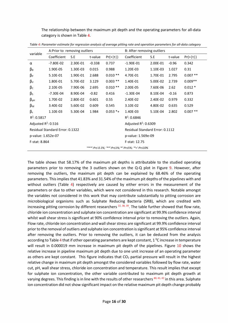
The relationship between the maximum pit depth and the operating parameters for all-data

category is shown in Table 4.

Table 4: Parameter estimate for regression analysis of average pitting rate and operation parameters for all-data category

variable A:Prior to removing outliers B: After removing outliers

Coefficient S.E t-value Pr(>|t|) Coefficient S.E t-value Pr(>|t|)

α -7.80E-02 2.30E-01 -0.338 0.737 -1.90E-01 2.00E-01 -0.96 0.342

βθ 1.90E-05 1.30E-03 0.015 0.988 1.20E-03 1.10E-03 1.027 0.31

βP 5.10E-01 1.90E-01 2.688 0.010 ** 4.70E-01 1.70E-01 2.795 0.007 **

βV 1.80E-01 5.70E-02 3.129 0.003 ** 1.40E-01 5.00E-02 2.739 0.009**

βC 2.10E-05 7.90E-06 2.695 0.010 ** 2.00E-05 7.60E-06 2.62 0.012 *

βS -7.30E-04 8.90E-04 -0.82 0.416 -1.30E-04 8.10E-04 -0.16 0.873

βpH 1.70E-02 2.80E-02 0.601 0.55 2.40E-02 2.40E-02 0.979 0.332

βW 3.40E-02 5.60E-02 0.609 0.545 3.10E-02 4.80E-02 0.635 0.529

βτ 1.10E-03 5.30E-04 1.984 0.053 *+ 1.40E-03 5.10E-04 2.802 0.007 **

R2: 0.5817 R2: 0.6846

Adjusted R2: 0.516 Adjusted R2: 0.6309

Residual Standard Error: 0.1322 Residual Standard Error: 0.1112

p-value: 1.652e-07 p-value: 1.569e-09

F-stat: 8.864 F-stat: 12.75

‘***’:Pr≤ 0.1%; ‘**’:Pr≤1%;‘*’:Pr≤5%; ‘*+’:Pr≤10%

The table shows that 58.17% of the maximum pit depths is attributable to the studied operating

parameters prior to removing the 3 outliers shown on the Q-Q plot in Figure 9. However, after

removing the outliers, the maximum pit depth can be explained by 68.46% of the operating

parameters. This implies that 41.83% and 31.54% of the maximum pit depths of the pipelines with and

without outliers (Table 4) respectively are caused by either errors in the measurement of the

parameters or due to other variables, which were not considered in this research. Notable amongst

the variables not considered in this work that may contribute substantially to pitting corrosion are

microbiological organisms such as Sulphate Reducing Bacteria (SRB), which are credited with

increasing pitting corrosion by different researchers 22, 38, 39. The table further showed that flow rate,

chloride ion concentration and sulphate ion concentration are significant at 99.9% confidence interval

whilst wall shear stress is significant at 90% confidence interval prior to removing the outliers. Again,

Flow rate, chloride ion concentration and wall shear stress are significant at 99.9% confidence interval

prior to the removal of outliers and sulphate ion concentration is significant at 95% confidence interval

after removing the outliers. Prior to removing the outliers, it can be deduced from the analysis

according to Table 4 that if other operating parameters are kept constant, 1 0C increase in temperature

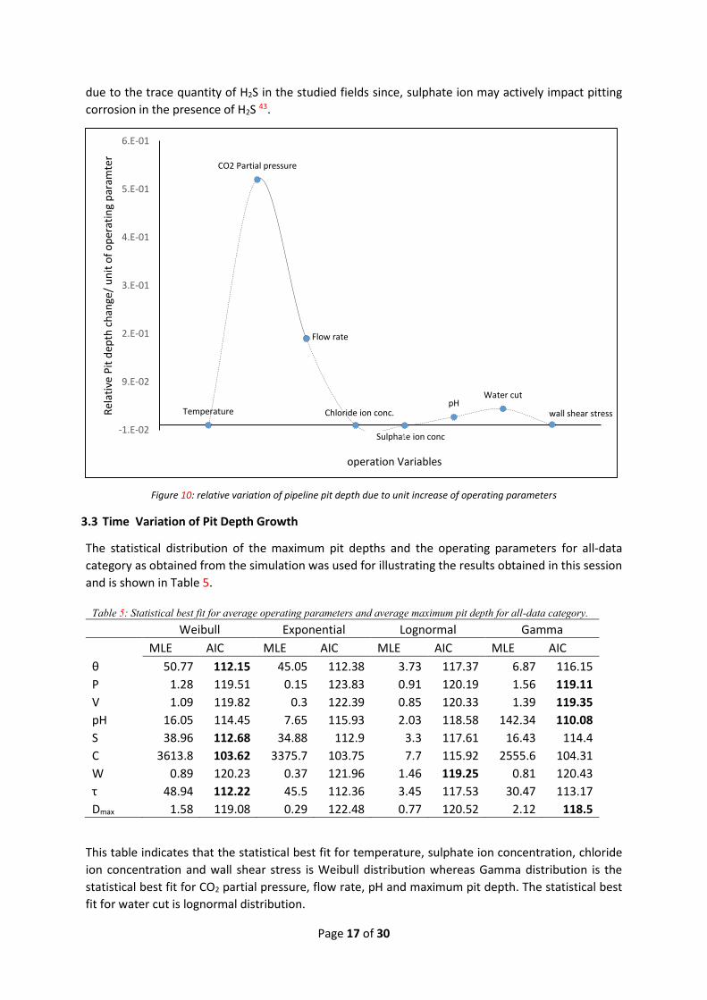
will result in 0.000019 mm increase in maximum pit depth of the pipelines. Figure 10 shows the

relative increase in pipeline maximum pit depth due to one unit increase of an operating parameter

as others are kept constant. This figure indicates that CO2 partial pressure will result in the highest

relative change in maximum pit depth amongst the considered variables followed by flow rate, water

cut, pH, wall shear stress, chloride ion concentration and temperature. This result implies that except

for sulphate ion concentration, the other variable contributed to maximum pit depth growth at

varying degrees. This finding is in line with the results of other researchers 40, 41, 42 in this area. Sulphate

ion concentration did not show significant impact on the relative maximum pit depth change probably

Page 17 of 30

due to the trace quantity of H2S in the studied fields since, sulphate ion may actively impact pitting

corrosion in the presence of H2S 43.

Figure 10: relative variation of pipeline pit depth due to unit increase of operating parameters

3.3 Time Variation of Pit Depth Growth

The statistical distribution of the maximum pit depths and the operating parameters for all-data

category as obtained from the simulation was used for illustrating the results obtained in this session

and is shown in Table 5.

Table 5: Statistical best fit for average operating parameters and average maximum pit depth for all-data category.

Weibull Exponential Lognormal Gamma

MLE AIC MLE AIC MLE AIC MLE AIC

θ 50.77 112.15 45.05 112.38 3.73 117.37 6.87 116.15

P 1.28 119.51 0.15 123.83 0.91 120.19 1.56 119.11

V 1.09 119.82 0.3 122.39 0.85 120.33 1.39 119.35

pH 16.05 114.45 7.65 115.93 2.03 118.58 142.34 110.08

S 38.96 112.68 34.88 112.9 3.3 117.61 16.43 114.4

C 3613.8 103.62 3375.7 103.75 7.7 115.92 2555.6 104.31

W 0.89 120.23 0.37 121.96 1.46 119.25 0.81 120.43

τ 48.94 112.22 45.5 112.36 3.45 117.53 30.47 113.17

Dmax 1.58 119.08 0.29 122.48 0.77 120.52 2.12 118.5

This table indicates that the statistical best fit for temperature, sulphate ion concentration, chloride

ion concentration and wall shear stress is Weibull distribution whereas Gamma distribution is the

statistical best fit for CO2 partial pressure, flow rate, pH and maximum pit depth. The statistical best

fit for water cut is lognormal distribution.

Temperature

CO2 Partial pressure

Flow rate

Chloride ion conc.

Sulphate ion conc

pHWater cut

wall shear stress

-1.E-02

9.E-02

2.E-01

3.E-01

4.E-01

5.E-01

6.E-01

0 1 2 3 4 5 6 7 8 9

Rel

ativ

e P

it d

epth

ch

ange

/ u

nit

of

op

erat

ing

par

amte

r

operation Variables

Page 18 of 30

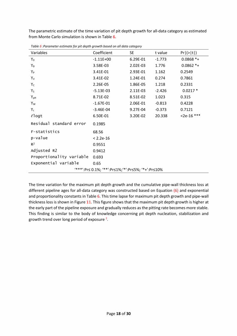
The parametric estimate of the time variation of pit depth growth for all-data category as estimated

from Monte Carlo simulation is shown in Table 6.

Table 6 :Parameter estimate for pit depth growth based on all data category

Variables Coefficient SE t value Pr|(>|t|)

ϒ0 -1.11E+00 6.29E-01 -1.773 0.0868 *+

ϒθ 3.58E-03 2.02E-03 1.776 0.0862 *+

ϒP 3.41E-01 2.93E-01 1.162 0.2549

ϒV 3.41E-02 1.24E-01 0.274 0.7861

ϒC 2.26E-05 1.86E-05 1.218 0.2331

ϒS -5.13E-03 2.11E-03 -2.426 0.0217 *

ϒpH 8.71E-02 8.51E-02 1.023 0.315

ϒW -1.67E-01 2.06E-01 -0.813 0.4228

ϒτ -3.46E-04 9.27E-04 -0.373 0.7121

ℓlogt 6.50E-01 3.20E-02 20.338 <2e-16 ***

Residual standard error 0.1985

F-statistics 68.56

p-value < 2.2e-16

R2 0.9551

Adjusted R2 0.9412

Proportionality variable 0.693

Exponential variable 0.65

‘***’:Pr≤ 0.1%; ‘**’:Pr≤1%;‘*’:Pr≤5%; ‘*+’:Pr≤10%

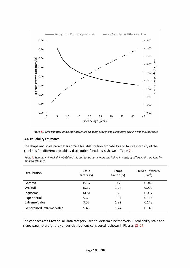
The time variation for the maximum pit depth growth and the cumulative pipe-wall thickness loss at

different pipeline ages for all-data category was constructed based on Equation (6) and exponential

and proportionality constants in Table 6. This time lapse for maximum pit depth growth and pipe-wall

thickness loss is shown in Figure 11. This figure shows that the maximum pit depth growth is higher at

the early part of the pipeline exposure and gradually reduces as the pitting rate becomes more stable.

This finding is similar to the body of knowledge concerning pit depth nucleation, stabilization and

growth trend over long period of exposure 2.

Page 19 of 30

Figure 11: Time variation of average maximum pit depth growth and cumulative pipeline wall thickness loss

3.4 Reliability Estimates

The shape and scale parameters of Weibull distribution probability and failure intensity of the

pipelines for different probability distribution functions is shown in Table 7.

Table 7: Summary of Weibull Probability Scale and Shape parameters and failure intensity of different distributions for all-data category

Distribution Scale

factor (ν) Shape

factor (ϕ) Failure intensity

(yr-1)

Gamma 15.57 0.7 0.040

Weibull 15.57 1.24 0.093

lognormal 14.81 1.25 0.097

Exponential 9.69 1.07 0.115

Extreme Value 9.57 1.22 0.143

Generalized Extreme Value 9.48 1.24 0.145

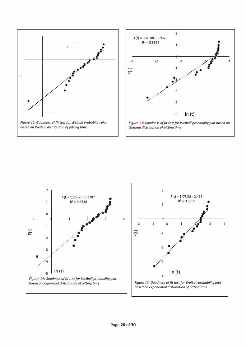
The goodness of fit test for all data category used for determining the Weibull probability scale and

shape parameters for the various distributions considered is shown in Figures 12 -17.

0.00

1.00

2.00

3.00

4.00

5.00

6.00

7.00

8.00

9.00

0.00

0.10

0.20

0.30

0.40

0.50

0.60

0.70

0.80

0 5 10 15 20 25 30 35 40 45

cum

ula

tive

pit

dep

th (

mm

)

Pit

dep

th g

row

th r

ate

(mm

/yr)

Pipeline age (years)

Average max Pit depth growth rate Cum pipe-wall thickness loss

Page 20 of 30

Figure 12: Goodness of fit test for Weibull probability plot based on Weibull distribution of pitting time

F(t) = 0.7038t - 1.9323R² = 0.8669

-5

-4

-3

-2

-1

0

1

2

-4 -2 0 2 4

F(t)

ln (t)

Figure 13: Goodness of fit test for Weibull probability plot based on Gamma distribution of pitting time

F(t)= 1.2537t - 3.3787R² = 0.9338

-5

-4

-3

-2

-1

0

1

2

-1 0 1 2 3 4

F(t)

ln (t)

Figure 14: Goodness of fit test for Weibull probability plot based on lognormal distribution of pitting time

F(t) = 1.0713t - 2.433R² = 0.9559

-4

-3

-2

-1

0

1

2

-2 -1 0 1 2 3 4

F(t)

ln (t)

Figure 15: Goodness of fit test for Weibull probability plot based on exponential distribution of pitting time

Page 21 of 30

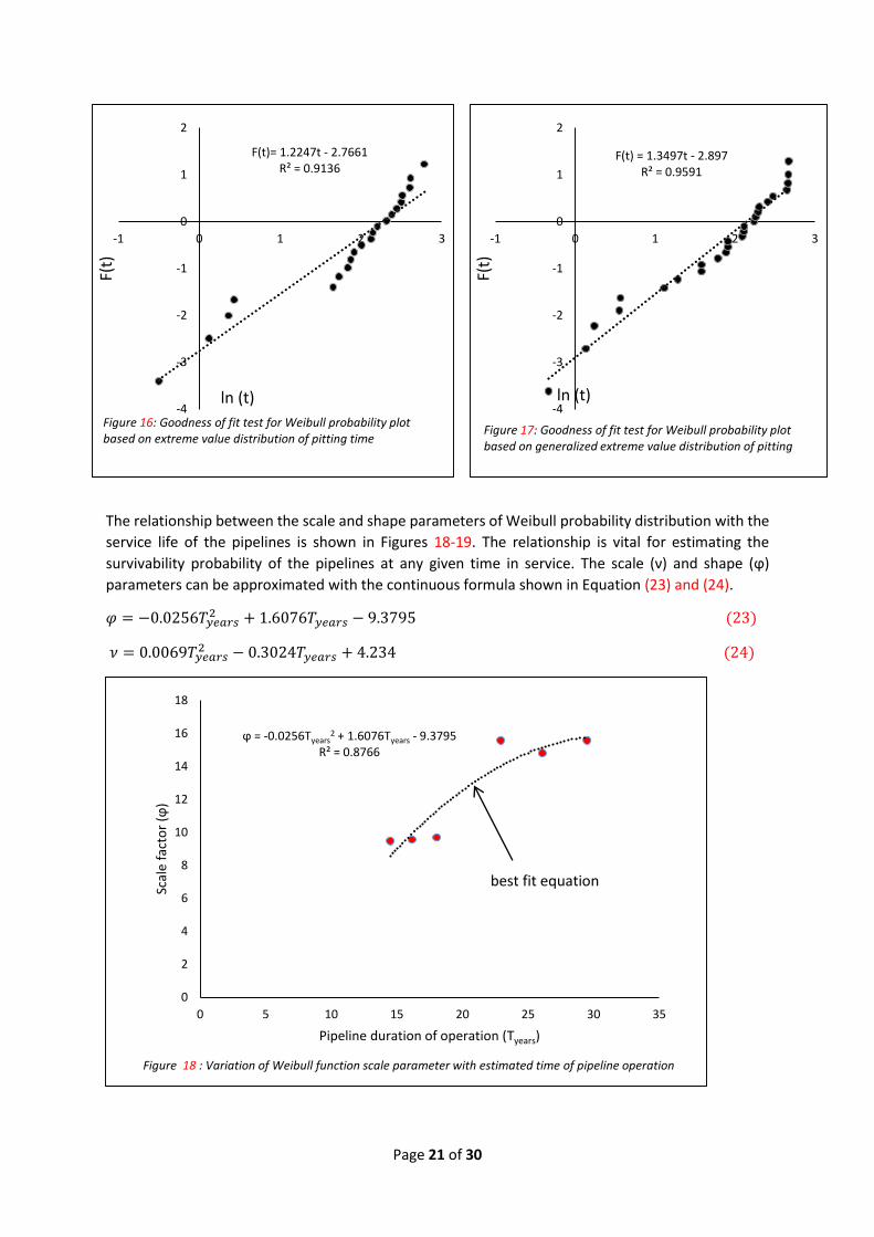
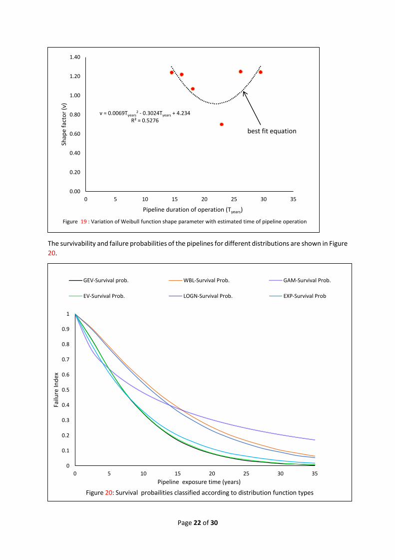
The relationship between the scale and shape parameters of Weibull probability distribution with the

service life of the pipelines is shown in Figures 18-19. The relationship is vital for estimating the

survivability probability of the pipelines at any given time in service. The scale (ν) and shape (ϕ)

parameters can be approximated with the continuous formula shown in Equation (23) and (24).

𝜑 = −0.0256𝑇𝑦𝑒𝑎𝑟𝑠2 + 1.6076𝑇𝑦𝑒𝑎𝑟𝑠 − 9.3795 (23)

𝜈 = 0.0069𝑇𝑦𝑒𝑎𝑟𝑠2 − 0.3024𝑇𝑦𝑒𝑎𝑟𝑠 + 4.234 (24)

F(t)= 1.2247t - 2.7661R² = 0.9136

-4

-3

-2

-1

0

1

2

-1 0 1 2 3

F(t)

ln (t)

Figure 16: Goodness of fit test for Weibull probability plot based on extreme value distribution of pitting time

F(t) = 1.3497t - 2.897R² = 0.9591

-4

-3

-2

-1

0

1

2

-1 0 1 2 3

F(t)

ln (t)

Figure 17: Goodness of fit test for Weibull probability plot based on generalized extreme value distribution of pitting

ϕ = -0.0256Tyears2 + 1.6076Tyears - 9.3795

R² = 0.8766

0

2

4

6

8

10

12

14

16

18

0 5 10 15 20 25 30 35

Scal

e fa

cto

r (ϕ

)

Pipeline duration of operation (Tyears)

Figure 18 : Variation of Weibull function scale parameter with estimated time of pipeline operation

best fit equation

Page 22 of 30

The survivability and failure probabilities of the pipelines for different distributions are shown in Figure

20.

ν = 0.0069Tyears2 - 0.3024Tyears + 4.234

R² = 0.5276

0.00

0.20

0.40

0.60

0.80

1.00

1.20

1.40

0 5 10 15 20 25 30 35

Shap

e fa

cto

r (ν

)

Pipeline duration of operation (Tyears)

Figure 19 : Variation of Weibull function shape parameter with estimated time of pipeline operation

best fit equation

0

0.1

0.2

0.3

0.4

0.5

0.6

0.7

0.8

0.9

1

0 5 10 15 20 25 30 35

Failu

re In

dex

Pipeline exposure time (years)

GEV-Survival prob. WBL-Survival Prob. GAM-Survival Prob.

EV-Survival Prob. LOGN-Survival Prob. EXP-Survival Prob

Figure 20: Survival probailities classified according to distribution function types

Page 23 of 30

This figure indicates that 80% of the pipe wall thickness will be lost after 13.99 years based on

generalized extreme value distribution whilst extreme value, exponential, lognormal, Weibull and

Gamma distributions will have the same 80% loss of pipe wall thickness lost in 14.20 years, 15.09

years, 21.70 years, 22.80 years and 30.57 years respectively.

4.0 Application

The application of this model is on Magnetic Flux Leakage (MFL) in-line inspection (ILI) data of a 3700m

long API X52 transmission pipeline having 8.7 mm nominal wall thickness and 203.2 mm external

diameter. This pipeline was commissioned in December 1994 and was inspected in August 2012 with

magnetic flux leakage in-line inspection (ILI) technique. The inspection produced a total of 1037 pit

depths samples that ranged from 10% to 60% of the nominal pipe-wall thickness of the pipeline.

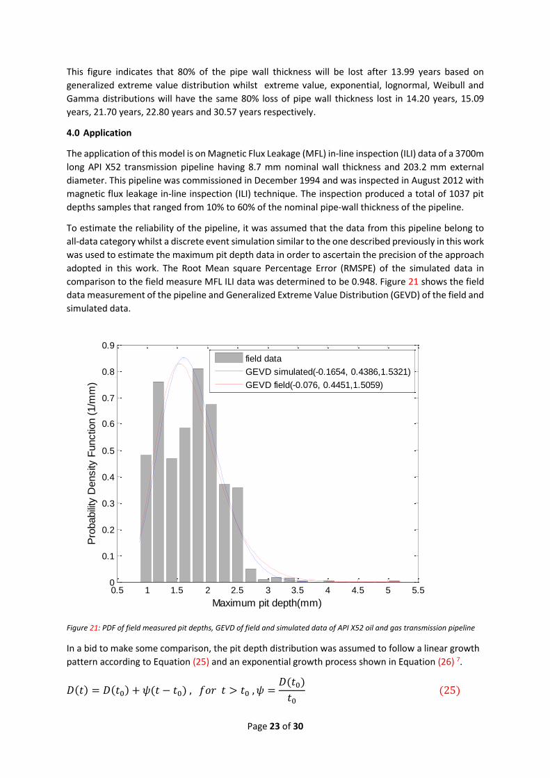
To estimate the reliability of the pipeline, it was assumed that the data from this pipeline belong to

all-data category whilst a discrete event simulation similar to the one described previously in this work

was used to estimate the maximum pit depth data in order to ascertain the precision of the approach

adopted in this work. The Root Mean square Percentage Error (RMSPE) of the simulated data in

comparison to the field measure MFL ILI data was determined to be 0.948. Figure 21 shows the field

data measurement of the pipeline and Generalized Extreme Value Distribution (GEVD) of the field and

simulated data.

Figure 21: PDF of field measured pit depths, GEVD of field and simulated data of API X52 oil and gas transmission pipeline

In a bid to make some comparison, the pit depth distribution was assumed to follow a linear growth

pattern according to Equation (25) and an exponential growth process shown in Equation (26) 7.

𝐷(𝑡) = 𝐷(𝑡0) + 𝜓(𝑡 − 𝑡0) , 𝑓𝑜𝑟 𝑡 > 𝑡0 , 𝜓 =𝐷(𝑡0)

𝑡0 (25)

0.5 1 1.5 2 2.5 3 3.5 4 4.5 5 5.50

0.1

0.2

0.3

0.4

0.5

0.6

0.7

0.8

0.9

Maximum pit depth(mm)

Pro

babili

ty D

ensity

Functio

n (

1/m

m)

field data

GEVD simulated(-0.1654, 0.4386,1.5321)

GEVD field(-0.076, 0.4451,1.5059)

Page 24 of 30

𝐷(𝑡0) = 𝐷(𝑡) (1 − 𝑒−(

𝑡0−𝑡𝑖𝑛𝑖𝑡−𝑡0

)) (26)

where D(t0) represents pit depth measured at time of inspection t0, D(t) represents future pit depth at

time t, tini represents the time of pitting initiation, which has been assumed to be zero in this work and

ψ represents the pitting rate which is determined as a function of the pit depth at time of inspection

and age of the pipeline.

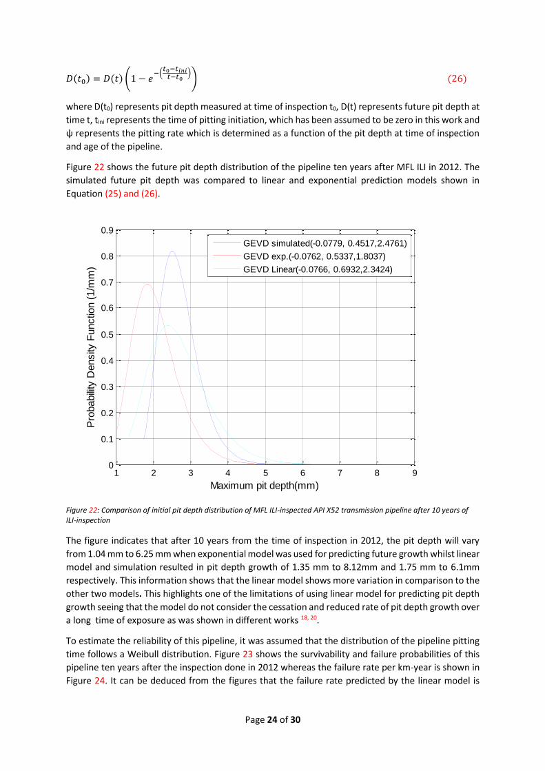
Figure 22 shows the future pit depth distribution of the pipeline ten years after MFL ILI in 2012. The

simulated future pit depth was compared to linear and exponential prediction models shown in

Equation (25) and (26).

Figure 22: Comparison of initial pit depth distribution of MFL ILI-inspected API X52 transmission pipeline after 10 years of ILI-inspection

The figure indicates that after 10 years from the time of inspection in 2012, the pit depth will vary

from 1.04 mm to 6.25 mm when exponential model was used for predicting future growth whilst linear

model and simulation resulted in pit depth growth of 1.35 mm to 8.12mm and 1.75 mm to 6.1mm

respectively. This information shows that the linear model shows more variation in comparison to the

other two models. This highlights one of the limitations of using linear model for predicting pit depth

growth seeing that the model do not consider the cessation and reduced rate of pit depth growth over

a long time of exposure as was shown in different works 18, 20.

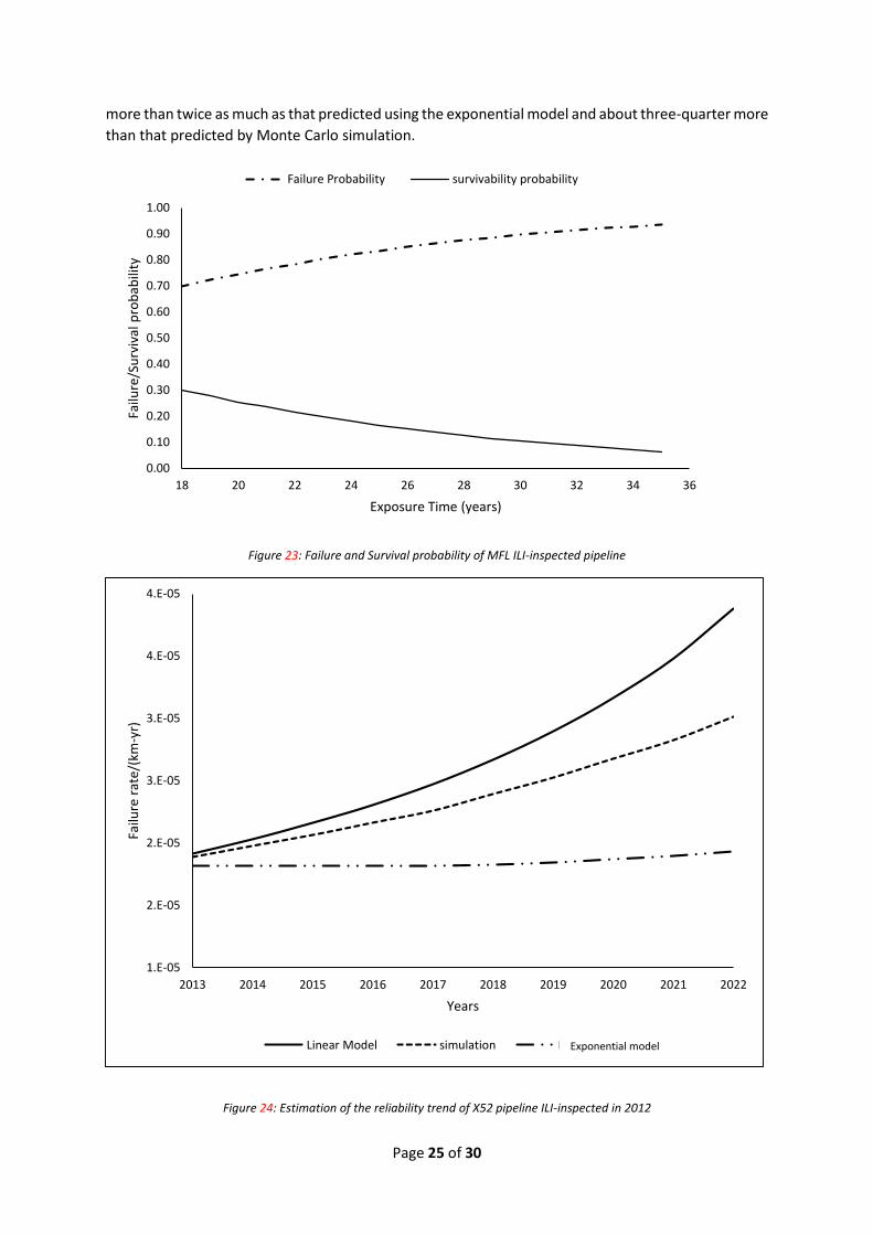
To estimate the reliability of this pipeline, it was assumed that the distribution of the pipeline pitting

time follows a Weibull distribution. Figure 23 shows the survivability and failure probabilities of this

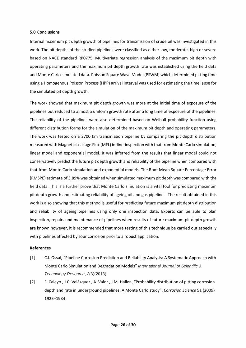
pipeline ten years after the inspection done in 2012 whereas the failure rate per km-year is shown in

Figure 24. It can be deduced from the figures that the failure rate predicted by the linear model is

1 2 3 4 5 6 7 8 90

0.1

0.2

0.3

0.4

0.5

0.6

0.7

0.8

0.9

Maximum pit depth(mm)

Pro

babili

ty D

ensity

Functio

n (

1/m

m)

GEVD simulated(-0.0779, 0.4517,2.4761)

GEVD exp.(-0.0762, 0.5337,1.8037)

GEVD Linear(-0.0766, 0.6932,2.3424)

Page 25 of 30

more than twice as much as that predicted using the exponential model and about three-quarter more

than that predicted by Monte Carlo simulation.

Figure 23: Failure and Survival probability of MFL ILI-inspected pipeline

Figure 24: Estimation of the reliability trend of X52 pipeline ILI-inspected in 2012

0.00

0.10

0.20

0.30

0.40

0.50

0.60

0.70

0.80

0.90

1.00

18 20 22 24 26 28 30 32 34 36

Failu

re/S

urv

ival

pro

bab

ility

Exposure Time (years)

Failure Probability survivability probability

1.E-05

2.E-05

2.E-05

3.E-05

3.E-05

4.E-05

4.E-05

2013 2014 2015 2016 2017 2018 2019 2020 2021 2022

Failu

re r

ate/

(km

-yr)

Years

Linear Model simulation PredictedExponential model

Page 26 of 30

5.0 Conclusions

Internal maximum pit depth growth of pipelines for transmission of crude oil was investigated in this

work. The pit depths of the studied pipelines were classified as either low, moderate, high or severe

based on NACE standard RP0775. Multivariate regression analysis of the maximum pit depth with

operating parameters and the maximum pit depth growth rate was established using the field data

and Monte Carlo simulated data. Poisson Square Wave Model (PSWM) which determined pitting time

using a Homogenous Poisson Process (HPP) arrival interval was used for estimating the time lapse for

the simulated pit depth growth.

The work showed that maximum pit depth growth was more at the initial time of exposure of the

pipelines but reduced to almost a uniform growth rate after a long time of exposure of the pipelines.

The reliability of the pipelines were also determined based on Weibull probability function using

different distribution forms for the simulation of the maximum pit depth and operating parameters.

The work was tested on a 3700 km transmission pipeline by comparing the pit depth distribution

measured with Magnetic Leakage Flux (MFL) in-line-inspection with that from Monte Carlo simulation,

linear model and exponential model. It was inferred from the results that linear model could not

conservatively predict the future pit depth growth and reliability of the pipeline when compared with

that from Monte Carlo simulation and exponential models. The Root Mean Square Percentage Error

(RMSPE) estimate of 3.89% was obtained when simulated maximum pit depth was compared with the

field data. This is a further prove that Monte Carlo simulation is a vital tool for predicting maximum

pit depth growth and estimating reliability of ageing oil and gas pipelines. The result obtained in this

work is also showing that this method is useful for predicting future maximum pit depth distribution

and reliability of ageing pipelines using only one inspection data. Experts can be able to plan

inspection, repairs and maintenance of pipelines when results of future maximum pit depth growth

are known however, it is recommended that more testing of this technique be carried out especially

with pipelines affected by sour corrosion prior to a robust application.

References

[1] C.I. Ossai, “Pipeline Corrosion Prediction and Reliability Analysis: A Systematic Approach with

Monte Carlo Simulation and Degradation Models” International Journal of Scientific &

Technology Research, 2(3)(2013)

[2] F. Caleyo , J.C. Velázquez , A. Valor , J.M. Hallen, “Probability distribution of pitting corrosion

depth and rate in underground pipelines: A Monte Carlo study”, Corrosion Science 51 (2009)

1925–1934

Page 27 of 30

[3] R. E. Melchers, “Extreme value statistics and long-term marine pitting corrosion of steel”,

Probabilistic Engineering Mechanics 23 (4) (2008) 482-488

[4] ASME, Manual for determining the remaining strength of corroded pipelines. American

Society of Mechanical Engineers, B31G, New York, 2009.

[5] R. Owen, V. Chauhan, D. Pipet, G. Morgan, “Assessment of corrosion damage in pipelines

with low toughness”, In 14th Biennial joint technical meeting on pipeline research, Berlin

(2003).

[6] G. Engelhardt, D. D. Macdonald, “Deterministic Prediction of Pit Depth Distribution”,

Corrosion 54 (6) (1998) 469-479

[7] C. G. Soares, Y. Garbatov, “Reliability of maintained, corrosion protected plates subjected to

non-linear corrosion and compressive loads” Marine Structures 12 (1999) 425-445

[8] J. L. Alamilla, E. Sosa, "Stochastic modelling of corrosion damage propagation in active sites

from field inspection data" Corrosion Science 50(7)(2008)1811-1819.

[9] S. Zhang, W. Zhou, H. Qin, “Inverse Gaussian process-based corrosion growth model for

energy pipelines considering the sizing error in inspection data”, Corrosion Science 73 (2013)

309-320

[10] A. Valor, F. Caleyo, J. M. Hallen, J. C. Velázquez, ”Reliability assessment of buried pipelines

based on different corrosion rate models”, Corrosion Science 66(2013) 78-87.

[11] A. Valor, F. Caleyo, D. Rivas, J.M. Hallen, “Stochastic approach to pitting-corrosion-extreme

modelling in low-carbon steel”, Corrosion Science 52(3) (2010) 910-915.

[12] J. C. Velazquez, A. Valor, F. Caleyo, V. Venegas, J. H. Espina-Hernandez, J. M. Hallen, M.R

Lopez, “Pitting corrosion models improve integrity management, reliability”, Oil and Gas

Journal, 107(28) (2009)56-62.

[13] S. Zhang, W. Zhou, “System reliability of corroding pipelines considering stochastic process-

based models for defect growth and internal pressure”, International Journal of Pressure

Vessels and Piping 111-112 (2013) 120-130

[14] E. S. Rodriguez III, J. W. Provan,” Part II: Development of a general failure control system for

estimating the reliability of deteriorating structures”, Corrosion 45(3) (1989)193-206.

[15] A. Valor, F. Caleyo, L. Alfonso, J. Vidal,J. M. Hallen, “Statistical Analysis of Pitting Corrosion

Field Data and Their Use for Realistic Reliability Estimations in Non-Piggable Pipeline

Systems”, Corrosion In-Press (2014)

[16] A. K. Sheikh, J. K. Boah, D. A. Hansen, “Statistical Modeling of Pitting Corrosion and Pipeline

Reliability”, Corrosion 46(3) (1990) 190-197.

Page 28 of 30

[17] M. H. Mohd, J. K. Paik, “Investigation of the corrosion progress characteristics of offshore

subsea oil well tubes”, Corrosion Science 67 (2013) 130-141.

[18] F. A. V. Bazan, A. T. Beck, “Stochastic process corrosion growth models for pipeline

reliability”, Corrosion Science 74(2013) 50-58.

[19] Y. Katano, K. Miyata, H. Shimizu, T. Isogai, “Predictive Model for Pit Growth on Underground

Pipes”, Corrosion 59(2) (2003) 155-161.

[20] J. C. Velazquez, F. Caleyo, A. Valor, J.M. Hallen, “Predictive model for pitting corrosion in

buried oil and gas pipelines”, Corrosion 65(5) (2009) 332-342.

[21] R.E. Melchers, “Estimating uncertainty in maximum pit depth from limited observational

data”, Corrosion Engineering Science and Technology 45(3) (2010) 240-248.

[22] R. E. Melchers, “Extreme value statistics and long-term marine pitting corrosion of steel”,

Probabilistic Engineering Mechanics 23(4) (2008) 482-488.

[23] P. J. Laycock, R. A. Cottis, P. A. Scarf, “Extrapolation of Extreme Pit Depths in Space and

Time”, J. Electrochem. Soc. 137(1) (1990).

[24] M. Chookah, M. Nuhi, M. Modarres, "A probabilistic physics-of-failure model for prognostic

health management of structures subject to pitting and corrosion-fatigue." Reliability

Engineering & System Safety 96(12) (2011)1601-1610.

[25] J. Hu, Y. Tian, H. Teng, L. Yu, M. Zheng, "The probabilistic life time prediction model of oil

pipeline due to local corrosion crack", Theoretical and Applied Fracture Mechanics

70(0)(2014) 10-18.

[26] S. Zhang, W. Zhou, "Bayesian dynamic linear model for growth of corrosion defects on

energy pipelines." Reliability Engineering & System Safety 128(0) (2014) 24-31.

[27] S. Hasan, F. Khan, S. Kenny, "Probability assessment of burst limit state due to internal

corrosion", International Journal of Pressure Vessels and Piping 89(0) (2012) 48-58.

[28] D. W. Shoesmith, P. Taylor, M.G. Bailey and D.G. Owen, “The Formation of Ferrous

Monosulfide Polymorphs During the Corrosion of Iron by Aqueous Hydrogen Sulfide at

21oC”, J. Electrochemical Soc., p. 1007, 1980

[29] L. Smith and B. Craig, “Corrosion mechanisms and material performance in environments

containing hydrogen sulfide and elemental sulphur”, SACNUC Workshop 22nd and 23rd

October, 2008, Brussels

[30] J. Dawson, K. Bruce and D. G. John, “Corrosion risk assessment and safety management for

offshore processing facilities”, HSE books UK, 2001. Available from:

http://www.hse.gov.uk/research/otopdf/1999/oto99064.pdf 6/5/15.

Page 29 of 30

[31] NACE standard RP0775, Preparation, installation, analysis and interpretation of corrosion

coupons in oilfield operations, NACE international, Houston, TX. USA, 2005.

[32] M. Ahammed, “Probabilistic estimation of remaining life of a pipeline in the presence of

active corrosion defects”, International Journal of Pressure Vessels and Piping 75 (4) (1998)

321-329.

[33] M. Ahammed, R.E. Melchers, “Reliability estimation of pressurised pipelines subject to

localised corrosion defects”, International Journal of Pressure Vessels and Piping 69(3) (1996)

267-272.

[34] S. Li, S. Yu, H. Zeng, J. Li, R. Liang, “Predicting corrosion remaining life of underground

pipelines with a mechanically-based probabilistic model”, Journal of Petroleum Science and

Engineering 65(3-4) (2009) 162-166.

[35] F. Caleyo, J.L. González, J.M. Hallen, “A study on the reliability assessment methodology for

pipelines with active corrosion defects”, International Journal of Pressure Vessels and Piping

79(1) (2002) 77-86.

[36] A. W. Dawotola, P.H.A.J.M. van Gelder, J.J. Charima, J.K. Vrijling, “Estimation of failure rates

of crude product pipelines” Applications of Statistics and Probability in Civil Engineering –

Faber, Köhler & Nishijima (eds) Taylor & Francis Group, London, 2011

[37] M.D. Pandey, X. -X. Yuan, J. M. van Noortwijk, “The influence of temporal uncertainty of

deterioration on life-cycle management of structures”, Structure & Infrastructure

Engineering 5 (2009) 145–156.

[38] C. Chandrasatheesh, J. Jayapriya, R. P. George, U. K. Mudali, “Detection and Analysis of

Microbiologically Influenced Corrosion of 316 L Stainless Steel with Electrochemical Noise

Technique”, Engineering Failure Analysis 42 (2014), 133-42.

[39] Y. Chen, R. Howdyshell, S. Howdyshell, L. Ju, “Characterizing pitting corrosion caused by a

long-term starving sulfate-reducing bacterium surviving on carbon steel and effects of

surface roughness”, Corrosion In-Press, 2014

[40] S. Hassani, K. Roberts, S. Shirazi, J. Shadley, E. Rybicki, C. Joia, “Flow loop study of chloride

concentration effect on erosion, corrosion and erosion-corrosion of carbon steel in CO2

saturated systems”, Corrosion 68(2) (2012) .

[41] W. P. Jepson, R. Menezes, “The effects of oil viscosity on sweet corrosion in multiphase oil,

water/gas horizontal pipelines”, In: NACE International Conference Series, Corrosion/95,

paper 106, (1995).

Page 30 of 30

[42] R. Zhang, M. Gopal, W.P. Jepson, “Development of a mechanistic model for predicting

Corrosion rate in multiphase oil/water/gas flows”, In: NACE International Conference Series,

Corrosion /97, paper 601, (1997).

[43] S. Papavinasam, A. Doiron, and R. W. Revie, “Model to Predict Internal Pitting Corrosion of

Oil and Gas Pipelines”, Corrosion 66(3) (2010) 035006-035006-11.