Embed Size (px)
Citation preview

© Crown copyright Met Office
Estimation of Carbon Cycle Parameters in JULESDavid Pearson, Chris D. Jones, John K. HughesJULES Science Meeting, January 2009

© Crown copyright Met Office
Abstract/Summary
• We are improving the terrestrial carbon cycle parameters in JULES by tuning them so we can simulate flux tower measurements.
• The tuning method is variational data assimilation.
• The usual formulation of Var is not applicable.
• A different weighting of prior and observation terms is needed.

© Crown copyright Met Office
Contents
This presentation covers the following areas
• Data assimilation: states or parameters?
• Data assimilation: sequential or variational?
• Var: the cost function.
• Var for parameter estimation.
• Weighting for the correlated problem.
• Results.
• What next?
• Q and A.

© Crown copyright Met Office
Data assimilation: states or parameters?

© Crown copyright Met Office
Data assimilation: states or parameters?
• The state of a system is the set of relevant or interesting evolving variables. E.g.:
• the CO2 concentration field in the atmosphere;
• the salinity field in the ocean;
• the velocity field in either;
• the moisture content in soil layers.
• Parameters are the fixed numbers in a model, that control the state. E.g.:
• ksat in soil;
• q10 in soil or leaves.

© Crown copyright Met Office
Data assimilation: sequential or variational?

© Crown copyright Met Office
Data assimilation: sequential or variational?
• Sequential, e.g. the Kalman filter.

© Crown copyright Met Office
Data assimilation: sequential or variational?
• Variational, e.g. 4D-Var.

© Crown copyright Met Office
Data assimilation: sequential or variational?
• State vectors:
• Sequential DA naturally accommodates model error;
• Sequential DA does not naturally accommodate nonlinearity.
• Var does not naturally accommodate model error;
• Var naturally accommodates nonlinearity.
• Parameters:
• Parameters are fixed, but sequential DA allows them to change;
• Parameter-Var has fixed parameters;
• JULES is more suited to variational parameter estimation than sequential estimation.

© Crown copyright Met Office
Data assimilation: sequential or variational?
For parameter estimation in JULES, Var
beats sequential

© Crown copyright Met Office
Var: the cost function.

© Crown copyright Met Office
Var: the cost function.

© Crown copyright Met Office
Var for parameter estimation.

© Crown copyright Met Office
Var for parameter estimation.
© Crown copyright Met Office
Var for parameter estimation.
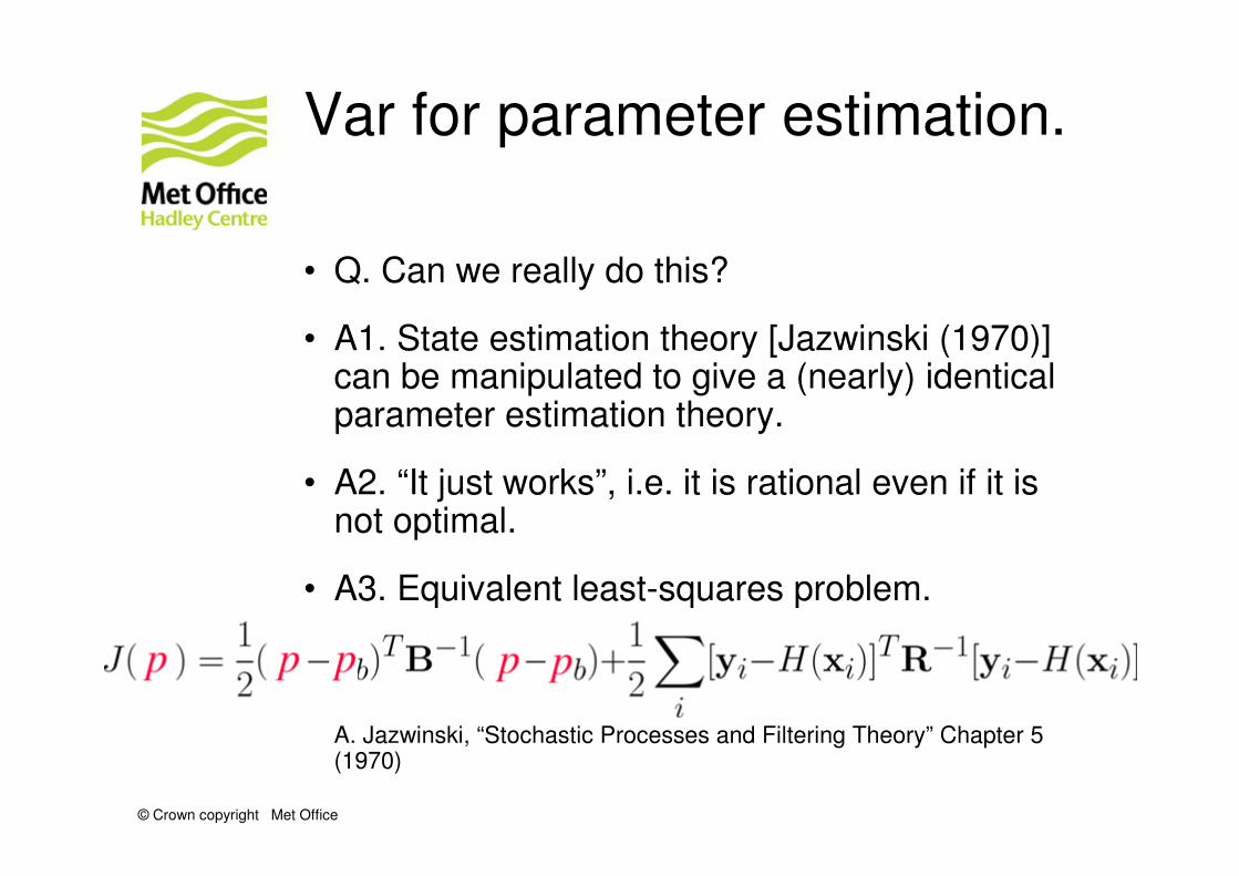
• Q. Can we really do this?
• A1. State estimation theory [Jazwinski (1970)] can be manipulated to give a (nearly) identical parameter estimation theory.
• A2. “It just works”, i.e. it is rational even if it is not optimal.
• A3. Equivalent least-squares problem.
A. Jazwinski, “Stochastic Processes and Filtering Theory” Chapter 5 (1970)

© Crown copyright Met Office
Parameter estimation for JULES.

© Crown copyright Met Office
Parameter estimation for JULES
• We want to optimise the terrestrial carbon cycle.
• Q. Which set of parameters do we work with?
• A1. Start with a set already studied [Booth (2009)];
• A2. Choose a few more;
• A3. Sensitivity analysis to find which subset had a strong effect on annual carbon pools and the timing and amplitude of seasonality.
[B. Booth et al., Increased importance of terrestrial carbon cycle feedbacks under global warming. Submitted to Nature (2009).]

© Crown copyright Met Office
Parameter estimation for JULES
Tlow and Tupp Maximum and minimum temperature constraints on
photosynthesis. These were covaried. [°C]
dQcrit Critical humidity deficit for photosynthesis. [kg water / kg air]
f0 Controller of stomatal carbon dioxide concentration. [unitless]
LAImin Minimum leaf area for vegetation areal expansion. [unitless]
nl0 Top leaf nitrogen concentration . [kg N / kg C]
q10,leaf Base for leaves in q10 model of respiration. [unitless]
q10,soil Base for soil in q10 model of respiration. [unitless]
α Soil albedo. [unitless]
ggrow Rate of leaf growth. [/360 days]
groot Turnover rate for root biomass. [/360 days]
gwood Turnover rate for woody biomass. [/360 days]

© Crown copyright Met Office
Parameter estimation for JULES
• p=(Tlow, dQcrit, f0, nl0, q10.leaf, q10.soil)
• Find p that minimises J(p) by the Nelder-Mead method over the 6-dimensional parameter space.
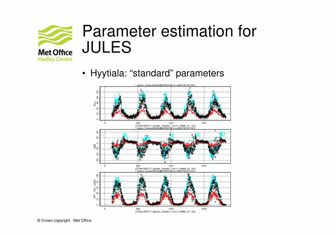
• Target functions: daily Reco, GPP and NEE over as many years as are available.
• (Note: NEE = -NEP)
© Crown copyright Met Office
Parameter estimation for JULES
• Hyytiala: “standard” parameters

© Crown copyright Met Office
Parameter estimation for JULES
• Hyytiala: “best” parameters
© Crown copyright Met Office
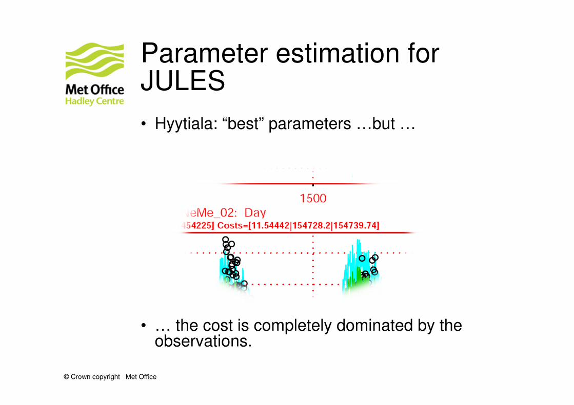
Parameter estimation for JULES
• Hyytiala: “best” parameters …but …
• … the cost is completely dominated by the observations.

© Crown copyright Met Office
Weighting for the correlated problem.

© Crown copyright Met Office
Weighting for the correlated problem.
• Var derivation assumes the system is 1st-order Markov: xk+1 = f(xk) + ek .
• OK for NWP and other autonomous systems.
• Not correct for systems driven by serially-correlated phenomena (e.g. the land surface is driven by weather and radiation).
• Correlated inputs → correlated outputs, containing less information.
• Therefore we should give less weight to observation terms.
• But how much?

© Crown copyright Met Office
Weighting for the correlated problem.
• Numerical experiment: weight prior and obs terms by chosen factors:
• R.fac is small.
• Only the ratio is important.

© Crown copyright Met Office
Weighting for the correlated problem.
• What happens when we vary the weights?

© Crown copyright Met Office
Weighting for the correlated problem.
• What happens when we vary the weights?

© Crown copyright Met Office
Weighting for the correlated problem.
• Changes in the relative weights cause changes in the results (of course!).
• The changes are systematic (good!)
• What are the best weights? (Difficult problem!)

© Crown copyright Met Office
Weighting for the correlated problem.
• Michalak et al., Maximum likelihood estimation of covariance parameters for Bayesian atmospheric trace gas surface flux inversions. JGR 110, D24107 (2005).
• NWP experience of correlated obs errors.
• Least-squares parameter estimation for time series.

© Crown copyright Met Office
Results.

© Crown copyright Met Office
Results
• Hyytiala, Finland: NL forest
© Crown copyright Met Office
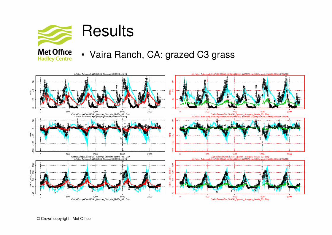
Results
• Vaira Ranch, CA: grazed C3 grass

© Crown copyright Met Office
Results
• Fort Peck, Montana: mixed C3/C4 grass

© Crown copyright Met Office
What next?

© Crown copyright Met Office
What next?
• Resolve the weighting problem.
• Gather more flux tower data over different PFTs.
• Take advantage of “JULES-TAF” (discussed by Tim Jupp in this session) for faster convergence.
• Examine the response of large-area carbon cycles (e.g. Europe or World).

© Crown copyright Met Office
Questions and answers

© Crown copyright Met Office
Abstract/Summary
• We are improving the terrestrial carbon cycle parameters in JULES by tuning them so we can simulate flux tower measurements.
• The tuning method is variational data assimilation.
• The usual formulation of Var is not applicable.
• A different weighting of prior and observation terms is needed.

© Crown copyright Met Office
Spare Slides

© Crown copyright Met Office
f0 and dqcrit
• ci is the internal partial pressure of CO2
• ca is the external partial pressure of CO2
• Γ is the photorespiration compensation point
• F0 is a tuning parameter
• D* is the humidity deficit at the leaf’s surface
• Dc is a tuning parameter