Estimation - Final Project

8/13/2019 Estimation - Final Project

http://slidepdf.com/reader/full/estimation-final-project 1/3

Heading Estimation of Fin Actuated Autonomous Underwater Vehicles

James Carrillo

University of Washington

AA 549: Estimation and Kalman Filtering

June 12, 2013

I. INTRODUCTION

The Fin Actuated Autonomous Underwater Vehicles used

in the the Nonlinear Dynamics and Control Lab at the

University Washington rely on both off-board and on-board

sensors to test different control methods and mathematical

models. State estimation and filtering greatly improve the

speed, accuracy, and response of any system dependent on

sensor data for control. A key on-board sensor used by

the vehicles is the 3D magnetic compass which provides

vehicle heading, pitch, and roll angles. The orientationinformation provided by the compass is used to calculate

tangential, normal, and binormal unit vectors which define

(at least partially) the system’s state. One problem with

estimating the vehicle’s state is the oscillatory motion of the

compass data due to the fin-actuated thrust. Estimation of

this oscillatory motion based on 3D compass measurements

will be attempted for a known vehicle path. The amplitude,

frequency, and phase shift of the heading oscillation will be

assumed as a static state.

II. MODEL

The assumed model for the 3D Compass measurement is

a sinusoidal function of constant amplitude, frequency, and

phase. The discrete time state equation for this model is

xk+1 = xk =

A

ω

φ

(1)

where A is amplitude, ω is frequency, and φ is the phase.

The measurement model is given by

˜ yk = x1 sin( x2t k + x3) + vk (2)

where yk is the measured value and vk is a zero-mean

Gaussian noise process. Due to the relatively slow velocity

and frequency of oscillation of the fish, a discrete-time modelwas assumed to sufficiently represent the system. Another

choice that would have been easily implemented and re-

duced computational effort is a continuous-discrete Extended

Kalman Filter. Had a requirement been to implement a

possible on-board filter, this choice would have been ideal.

Also, because the state being estimated is constant, other

nonlinear estimators can easily accomplish the same task. A

particle filter was chosen because it less susceptible to the

unmodeled dynamics that are commonly experienced in an

underwater environment[2].

III. DATA

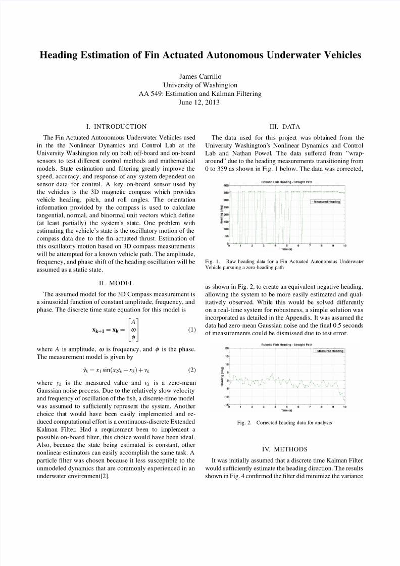
The data used for this project was obtained from the

University Washington’s Nonlinear Dynamics and Control

Lab and Nathan Powel. The data suffered from ”wrap-

around” due to the heading measurements transitioning from

0 to 359 as shown in Fig. 1 below. The data was corrected,

Fig. 1. Raw heading data for a Fin Actuated Autonomous UnderwaterVehicle pursuing a zero-heading path

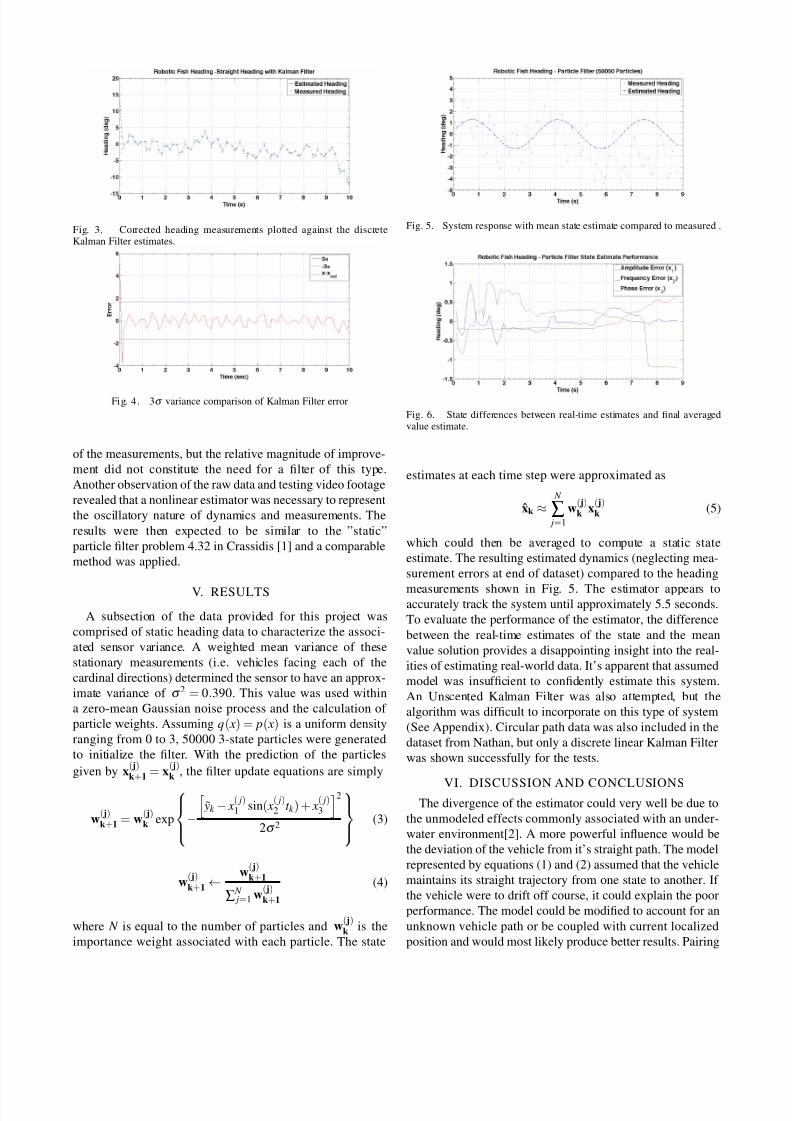
as shown in Fig. 2, to create an equivalent negative heading,

allowing the system to be more easily estimated and qual-

itatively observed. While this would be solved differently

on a real-time system for robustness, a simple solution was

incorporated as detailed in the Appendix. It was assumed the

data had zero-mean Gaussian noise and the final 0.5 seconds

of measurements could be dismissed due to test error.

Fig. 2. Corrected heading data for analysis

IV. METHODS

It was initially assumed that a discrete time Kalman Filter

would sufficiently estimate the heading direction. The results

shown in Fig. 4 confirmed the filter did minimize the variance



Fig. 3. Corrected heading measurements plotted against the discreteKalman Filter estimates.

Fi g. 4. 3σ variance comparison of Kalman Filter error

of the measurements, but the relative magnitude of improve-

ment did not constitute the need for a filter of this type.

Another observation of the raw data and testing video footage

revealed that a nonlinear estimator was necessary to represent

the oscillatory nature of dynamics and measurements. The

results were then expected to be similar to the ”static”

particle filter problem 4.32 in Crassidis [1] and a comparable

method was applied.

V. RESULTS

A subsection of the data provided for this project was

comprised of static heading data to characterize the associ-

ated sensor variance. A weighted mean variance of these

stationary measurements (i.e. vehicles facing each of the

cardinal directions) determined the sensor to have an approx-

imate variance of σ 2 = 0.390. This value was used within

a zero-mean Gaussian noise process and the calculation of

particle weights. Assuming q( x) = p( x) is a uniform density

ranging from 0 to 3, 50000 3-state particles were generated

to initialize the filter. With the prediction of the particles

given by x( j)k+1 = x

( j)k , the filter update equations are simply

w( j)k+1 = w

( j)k exp

−

˜ yk − x

( j)1 sin( x

( j)2 t k ) + x

( j)3

2

2σ 2

(3)

w( j)k+1←

w( j)k+1

∑ N j=1 w

( j)k+1

(4)

where N is equal to the number of particles and w( j)k is the

importance weight associated with each particle. The state

Fig. 5. System response with mean state estimate compared to measured .

Fig. 6. State differences between real-time estimates and final averagedvalue estimate.

estimates at each time step were approximated as

x̂k ≈

N

∑ j=1

w( j)k x

( j)k (5)

which could then be averaged to compute a static state

estimate. The resulting estimated dynamics (neglecting mea-

surement errors at end of dataset) compared to the heading

measurements shown in Fig. 5. The estimator appears toaccurately track the system until approximately 5.5 seconds.

To evaluate the performance of the estimator, the difference

between the real-time estimates of the state and the mean

value solution provides a disappointing insight into the real-

ities of estimating real-world data. It’s apparent that assumed

model was insufficient to confidently estimate this system.

An Unscented Kalman Filter was also attempted, but the

algorithm was difficult to incorporate on this type of system

(See Appendix). Circular path data was also included in the

dataset from Nathan, but only a discrete linear Kalman Filter

was shown successfully for the tests.

VI. DISCUSSION AND CONCLUSIONSThe divergence of the estimator could very well be due to

the unmodeled effects commonly associated with an under-

water environment[2]. A more powerful influence would be

the deviation of the vehicle from it’s straight path. The model

represented by equations (1) and (2) assumed that the vehicle

maintains its straight trajectory from one state to another. If

the vehicle were to drift off course, it could explain the poor

performance. The model could be modified to account for an

unknown vehicle path or be coupled with current localized

position and would most likely produce better results. Pairing



the results with a physical observance of the actual test would

also provide some more insight into environmental variability

or specific data points.

REFERENCES

[1] ”Optimal Estimation of Dynamic Systems”. ”CRC Press”, ”2012”.[2] K. A. M. et al”, “”geometric methods for modeling and control of free-

swimming fin-actuated underwater vehicles”,” ”IEEE Transactions on

Robotics”, ”2007”.

Documents

Estimation - Final Project