Estimating your soil erosion losses with the universal soil loss

UNIVERSITY OF

ILLINOIS LIBRARY

AT URBANA-CHAMPAIGN

ACES

NOTICE: Return or renew all Library Materlalsl The Minimum Fee for

each Lost Book is $50.00.

The person charging this material is responsible for

its return to the library from which it was withdrawnon or before the Latest Date stamped below.

Theft, mutilation, and underlining of books are reasons for discipli-

nary action and may result in dismissal from the University.

To renew call Telephone Center, 333-8400

UNIVERSITY OF ILLINOIS LIBRARY AT URBANA-CHAMPAIGN

L161—O-1096

MAR 2 8 2001

AGRICULTURE LIBRARY

Digitized by the Internet Archive

in 2011 with funding from

University of Illinois Urbana-Champaign

http://www.archive.org/details/estimatingyourso1220walk

. <II=^' • d0.(^30.7 , -_1 . /l/- "x^ô : ^- . '^Tc ,

• p 9 ...,,^' -..^1 -

5

J ..^4- \«%A^ \MW^M . '* ' ' '^

'.rtn Losseswi*

J CrtU Erosion i-"^ pv

=hh« UnWersalsort u ^

,

i ^ 1 d d_z: • ^- ' ^ ,•^^ ii diP tr Ij

^^ -A- JC- -A

J w M. • - ^^1 ^- ^^^^ #_ -4it -1

1 /• I.™,i„ « rf: - „ i „. , - _ ,

' A] 4i A^ ^^ ^ ^^ _!_# I^

1 1 1 ^f a\ W^ ' FT ^ rl*".^ x-sr*'^ ^—=^ ^ ^

^^Tl^ ^W^ , , ili^^JZ^ > V ^^ —.11 Y 4a^5 *^^4S^Î^-f7S^"•^»^•^ji #! ^^^^na!! Cooperative Extension ServiceCollege of Agriculture Circular 1220

University of Illinois at Urbana-Champaign IBBIBBIIIBBBBBBBBBBBBBBBBBBBBBBBBBBBBBBBBBBB

TABLE OF CONTENTS

Illinois Erosion Control Program 1

The Universal Soil Loss Equation (USEE) 1

Rainfall (R) Factor 2Soil Erodibility (K) Factor 2

Slope Length and Steepness (LS) Factor 3Cropping and Management (C) Factor 3Conservation Practices (P) Factor 5

Using the USEE 6

Working through Some Examples 6

Solving the USEE for C 7

Getting Help 7

Tables 8-16

Appendix: How to Make and Use a Slope Gauge 17

Table 1.

Table 2.

Table 3.

Table 4.

Table 5.

Table 6.

Table 7.

Table 8.

Table 9.

Table 10

Tables

Soil Erodibility (K) and Erosion Tolerance (T) Valuesfor Specific Illinois Soils 8

Soil Erodibility (K) Values for Certain General Soil Types 11

Slope Length and Steepness (LS) Values for Specific Combinationsof Length and Steepness 11

Cropping and Management (C) Values for Northern Illinois 12

Cropping and Management (C) Values for Central Illinois 13

Cropping and Management (C) Values for Southern Illinois 14

C Values for Permanent Pasture, Range, and Idle Land 15

C Values for Undisturbed Forest Land 15

Conservation Practices (P) Values for Contour Farmingand Contour Strip Cropping 16

Values Used in Determining P Values for Terraces Built on Contour andUsed in Combination with Contour Farming and Contour Strip Cropping ... 16

This circular was prepared by Robert D. Wall<er, Extension natural

resources specialist, and Robert A. Pope, former Extension agron-

omist, University of Illinois at Urbana-Champaign. The authors

would like to thank Steve Probst, Soil Conservation Service, for his

careful review and helpful suggestions.

Information in this circular is based on Agricultural Handbook 537 published by the Science and Education

Administration, U.S. Department of Agriculture, and generally corresponds with information contained in the

Soil Conservation Service's Illinois Technical Guide.

Excessive soil erosion occurs on 40 percent, or

9.6 million acres, of Illinois cropland. Erosion

on this land exceeds the soil loss tolerances of

one to five tons per acre annually, with a high of

over 50 tons per acre and an average of 1 1. 7 tons.

In addition, 23 percent, or 700,000 acres, of

pastureland and 16 percent, or 600,000 acres, of

woodland have excessive soil erosion.

The loss of valuable topsoil to erosion is

compounded by the loss of plant nutrients andorganic matter and by more difficulty in tilling

since the soil becomes increasingly clayey as

more subsoil is brought to the surface. But the

problems of erosion are not confined to farm-

land. The sediment that leaves fields often has

an adverse effect on the water quality andcondition of drainage ditches, lakes, reservoirs,

and streams. Many types of problems arise:

sediment decreases the storage capacity of lakes

and reservoirs, clogs streams and drainage

channels, causes deterioration of aquatic hab-

itats, increases water treatment costs, and car-

ries displaced plant nutrients.

Illinois Erosion Control Program

In response to the accelerated loss of soil

productivity and to the off-the-farm effects of

erosion, the state of Illinois has designed anerosion control program. The goal of this pro-

gram is to reduce annual soil erosion losses on

all agricultural land to one to five tons per acre

by the year 2000 depending upon the soil type.

This rate of erosion is considered the soil loss

tolerance level (the T value). Where erosion

exceeds the T value, soil is being lost so fast that

the land's natural productivity is being dimin-

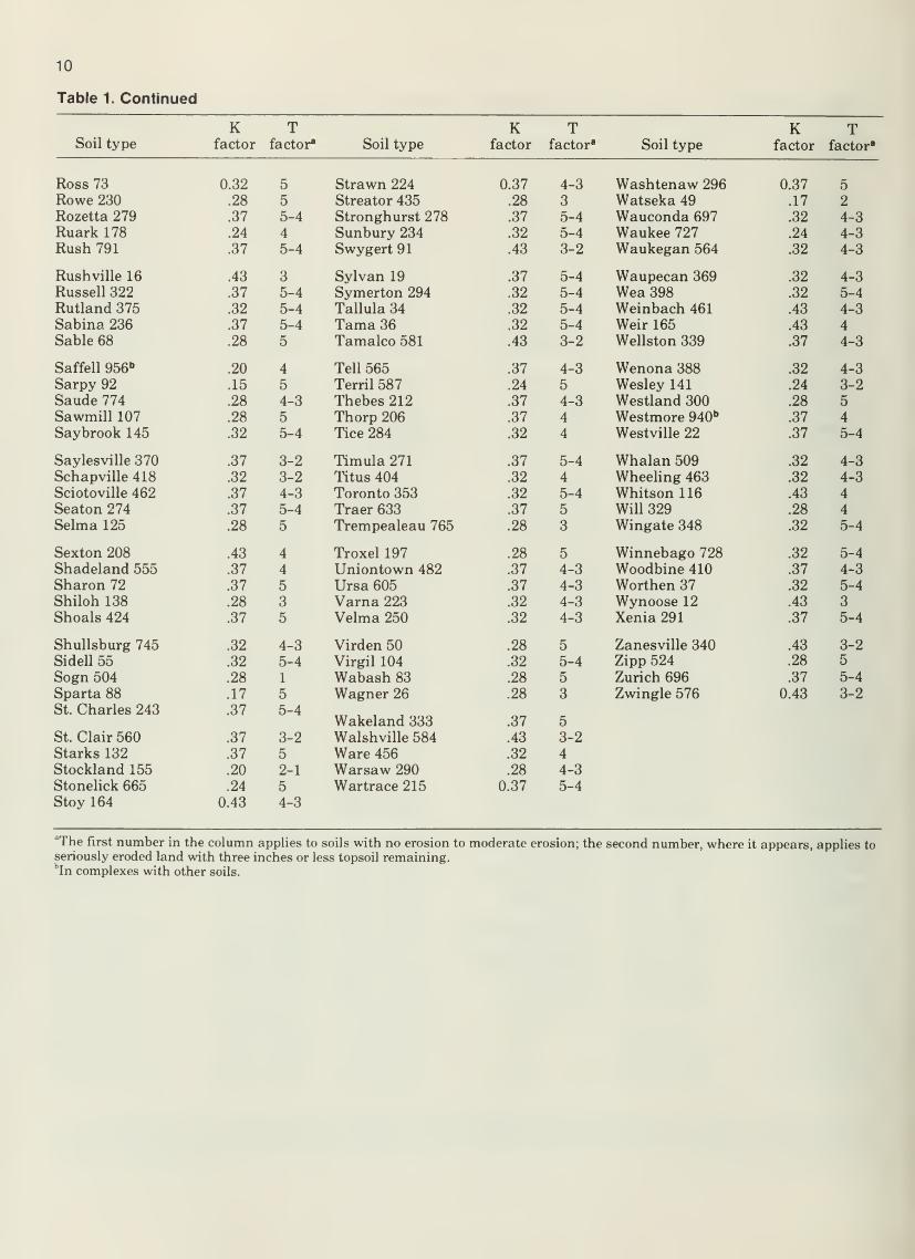
ished. Table 1 lists the T value for most Illinois

soils (all tables are given at the end of the text).

The erosion control program is divided into

intermediate goals, all leading up to the year

2000. To begin the program, the 98 soil andwater conservation districts in Illinois devel-

oped soil erosion standards for all soils in their

districts. The districts' standards, which wentinto effect on January 1, 1983, were required to

be at least as stringent as the state's guidelines,

although some districts developed standards

stricter than the state's guidelines.

The state's guidelines are as follows:

• By January 1, 1983, erosion on all farmlandcould not exceed four times the T value (4 to

20 tons per acre annually) established for

the soil type.

• By January 1, 1988, soil loss cannot exceed

two times the T value (2 to 10 tons per acre

annually). Where conservation tillage wouldsolve the erosion problem and the slope is

less than five percent, however, soil loss

must not exceed the T value (1 to 5 tons per

acre annually).

• By January 1 , 1 994, erosion on all farmlandcannot exceed one and a half times T (V/, to

1% tons per acre annually).

• By January 1 of the year 2000, erosion

cannot exceed the T value (1 to 5 tons per

acre annually) on any Illinois farmland.

Although the soil and water conservation dis-

tricts are delegated the task of administrating

the erosion control program, it is, as ofNovember,1983, still voluntary. There is, however, a clearly

defined complaint process. It is always possible

that the program will become mandatory if the

voluntary approach does not work.

The Universal Soil LossEquation (USLE)

The Universal Soil Loss Equation (USLE)provides a convenient way for you to estimatethe rate of soil loss on your land so that you cansee how that rate compares with your district's

standards. The USLE takes into account the

major factors that influence soil erosion by rain-

fall: rainfall patterns, soil types, slope steepness,

and management and conservation practices. It

was developed by the Agricultural ResearchService, the state experiment stations, and the

Soil Conservation Service (SCS), using research

data from many research stations, including

work at Dixon Springs, Urbana, and Elwood,Illinois. More than 10,000 plot years of datawere analyzed and used to develop the equationin the early 1960s. Additional data, mainly fromrainfall simulator plots, have been added to the

equation in the latest revision. Most of the

recent data covers conservation tillage, reducedtillage, till-plant, and no-till systems.

The USLE represents the average annualrate of soil loss due to splash, sheet, and rill

erosion. It does not estimate soil erosion fromgullies or stream banks or the amount of sedi-

ment reaching streams. Moreover, the equationonly gives the estimated average annual splash,

sheet, and rill erosion for the specific field

segment for which you have determined the

appropriate factors. It will not reflect the aver-

age soil erosion rate for the entire field unless

the segment you chose represents the field. In

general, however, you should not select a "repre-

sentative" field segment, but the field segmentwhere erosion is generally more severe. Takingestimates on several field segments will give

you a better idea of the scope of your erosion

problems. However, do not take an average of

the several estimates because that may maskthe severity of erosion on a particular segment.

The equation is simple to use. Once you havedetermined the values for each ofthe five factors,

you multiply them using a pocket calculator or,

if you prefer, pencil and paper. The equation is:

RXKXLSXCXP = A

where R — rainfall factor

K = soil erodibility factor

LS = length and steepness of slope factor

C = cropping and management factor

P = conservation practices factor

A = the computed average annual soil ero-

sion loss in tons per acre

Once you have determined A, you can com-

pare it with the T values in Table 1 and with

your Soil and Water Conservation District's

standards. You also can use the equation to

evaluate the effect that various changes in your

farming practices would have on your soil loss

rate. Keep in mind, however, that A is only as

accurate as the values that you have chosen for

the five factors. In general, if you have used

reasonable care in selecting the factors, A should

be within a range of plus or minus 20 percent of

your actual average annual erosion on the field

segment.

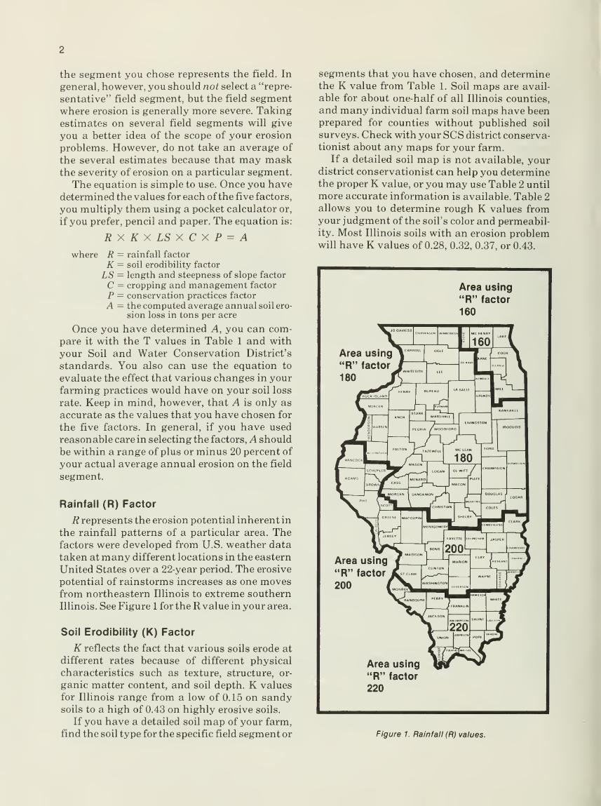
Rainfall (R) Factor

R represents the erosion potential inherent in

the rainfall patterns of a particular area. Thefactors were developed from U.S. weather data

taken at many different locations in the eastern

United States over a 22-year period. The erosive

potential of rainstorms increases as one movesfrom northeastern Illinois to extreme southern

Illinois. See Figure 1 for the R value in your area.

Soil Erodibility (K) Factor

K reflects the fact that various soils erode at

different rates because of different physical

characteristics such as texture, structure, or-

ganic matter content, and soil depth. K values

for Illinois range from a low of 0.15 on sandysoils to a high of 0.43 on highly erosive soils.

If you have a detailed soil map of your farm,

find the soil type for the specific field segment or

segments that you have chosen, and determinethe K value from Table 1. Soil maps are avail-

able for about one-half of all Illinois counties,

and many individual farm soil maps have beenprepared for counties without published soil

surveys. Check with your SCS district conserva-

tionist about any maps for your farm.

If a detailed soil map is not available, yourdistrict conservationist can help you determinethe proper K value, or you may use Table 2 until

more accurate information is available. Table 2

allows you to determine rough K values fromyour judgment of the soil's color and permeabil-ity. Most Illinois soils with an erosion problemwill have K values of 0.28, 0.32, 0.37, or 0.43.

Area using

"R" factor

160

Area using

"R" factor

180

Area using

"R" factor

200

Area using

"R" factor

220

Figure 1. Rainfall (R) values.

Slope Length and Steepness (LS) Factor

LS represents the erosive potential of a par-

ticular combination of slope length and slope

steepness. Slope length is not the distance from

the highest point in the field to the lowest point.

To determine slope length, you must walk the

field and determine where water will flow. Dis-

regard contour farming channels and concen-

trate on natural flow patterns. Once you haveidentified the natural flow patterns, determine

the point on the slope where the flow begins. Theslope length is then the distance from this point

to the point where (1) the slope gradient de-

creases enough that sediment deposition gener-

ally occurs, or (2) the runoff water becomes a

concentrated flow, or (3) the runoff enters a well-

defined channel, for example, part of a natural

drainage network or a constructed grass water-

way or terrace channel.* There is a tendency to

overestimate slope length. Slope lengths will

seldom be above 400 feet long on gentle slopes

and will usually be shorter on steeper slopes.

Slope steepness is expressed as a percentage.

The percentage of slope is the change in eleva-

tion between two points divided by the hori-

zontal distance between the two points times

100. For example, if the elevation change is 6

feet in a horizontal distance of 1 20 feet, the slope

has a 5 percent grade (6 ^ 120 X 100 = 5). Per-

cent slope can be determined with an engineer's

level, a hand level, a line or string level, or a

sighting board slope finder like the one on page19 (instructions for using it are on page 17).

Once you have determined slope length andsteepness, you can find the LS value in Table 3.

Please note that slope classifications given in

detailed soil maps should not be used; they are

too general. The slope length and steepness

must be determined on the specific segment of

the field where you are estimating soil loss, andthe LS value must be derived from Table 3.

Cropping and Management (C) Factor

C reflects the reduction in soil erosion that

will result from growing a crop as comparedwith leaving the land fallow. The amount of

*Where terraces are installed, the slope length is

usually the distance from the top of the terrace ridge

to the center of the next lower terrace channel. If the

terraces are built on the contour and used in conjunc-

tion with contour farming or contour strip cropping,

an additional P factor is used. See pages 5-6 for

calculating the P factor for terraces built on contour.

reduction depends upon the type of crop grown,

the cropping system, tillage practices, crop yield,

and residue management. Cropping and man-agement practices influence erosion potential

by the degree to which their combinations keep

the soil surface rough or covered with crop

residues or vegetation. C values range from a

high of 1.0 for continuous fallow (soil tilled to

permit no vegetation to grow) to a low of 0.003

for excellent grass cover. By determining R XK X LS for the field segment under examinationand multiplying that figure by various C values,

you can compare the soil erosion that you could

expect from different cropping and manage-ment practices (without the use of soil conserva-

tion practices).

There are many possible cropping and man-agement combinations. For example, almostany crop can be grown continuously or in

rotation with other crops, and additional soil

protection can be gained by seeding a cover crop

in the row crop late in the season. Soils can be

left rough with considerable storage capacity, or

they can be smoothed by secondary tillage. Cropresidues can be removed, left on the soil surface,

incorporated near the soil surface, or plowedunder. Even if crop residue is left on the surface,

it can be chopped or allowed to remain as it wasafter harvest.

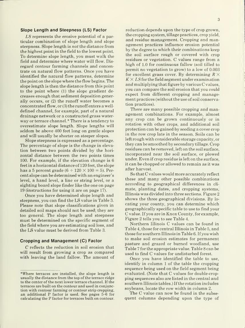
So that C values would more accurately reflect

these and many other possible combinationsaccording to geographical differences in cli-

mate, planting dates, and cropping systems,

Illinois was divided into three sections. Figure 2

shows the three geographical divisions. By lo-

cating your county, you can determine whichgeographically specific table to use to find your

C value. Ifyou are in Knox County, for example.Figure 2 tells you to see Table 4.

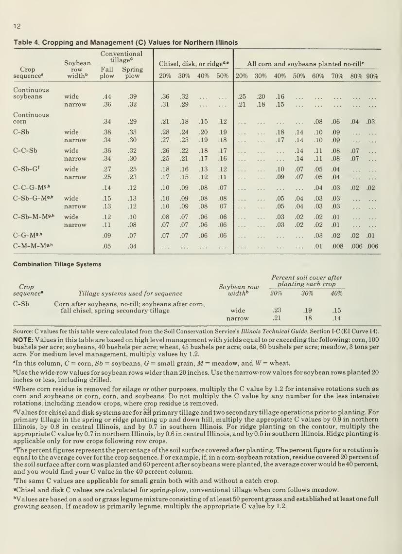
Northern Illinois C values can be found in

Table 4, those for central Illinois in Table 5, andthose for southern Illinois in Table 6. Ifyou wishto make soil erosion estimates for permanentpasture and grazed or burned woodland, use

Table 7 for the appropriate value. Table 8 can be

used to find C values for undisturbed forest.

Once you have identified the table to use,

identify in column 1 of the table the cropping

sequence being used on the field segment being

evaluated. (Note that C values for double-crop-

ping sequences also are listed in the central andsouthern Illinois tables.) If the rotation includes

soybeans, locate the row width in column 2.

The C value can now be found in the subse-

quent columns depending upon the type of

Northern

Illinois AreaUse Table 4

Central

Illinois AreaUse Table 5

Southern

Illinois Area

Use Table 6

Figure 2. Cropping and management (C) factor map.

tillage that is used—conventional, reduced, or

no-till. (Each table also lists C values for somemore common combinations of these tillage

systems. See your SCS district conservationist

if you are using other combinations.) Conven-tional tillage includes moldboard plowing, disk-

ing, planting, and cultivating. Reduced tillage

includes either a chisel plow or a disk as the

primary tillage tool, followed by a field culti-

vator or other secondary tillage tools that leave

a portion of the crop residue on the soil surface

after planting. No-till involves leaving the soil

surface nearly undisturbed and all crop residue

on the soil surface, thus providing maximumsoil erosion protection all season.

Ifyou are using conventional tillage, you canlook under either the "fall plow" or "springplow" column to determine your C value. If youare using a reduced tillage or no-till system,

however, you will first need to determine the

percentage ofresidue cover after planting before

finding your C value.

Residue soil surface cover after planting is

important because it provides soil protection

when the soil would otherwise be most vulner-

able to erosion: from seedbed preparation until

new crop growth provides soil cover. This timeperiod, when the ground is exposed to the ele-

ments, is also when the most intensive rains

usually occur.

There is a difference in the amount of residue

cover left on the soil surface by different crops

and how well this cover holds up under planting

operations. For example, a good field of corn

with a yield of over 100 bushels per acre will

leave about 90 to 95 percent of the soil surface

covered after harvest, while a good field of

soybeans with a yield of 40 to 45 bushels per acre

will leave about 80 to 85 percent. Because soy-

bean residue is more fragile, additional tillage

or travel over the field after harvest and during

planting will cover much more of the soybeanresidue than the corn residue.

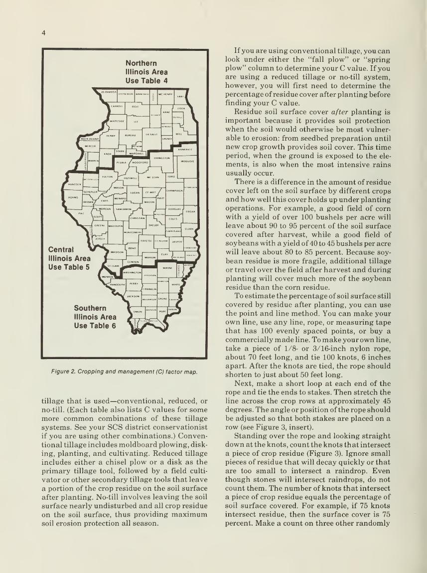
To estimate the percentage of soil surface still

covered by residue after planting, you can use

the point and line method. You can make yourown line, use any line, rope, or measuring tape

that has 100 evenly spaced points, or buy a

commercially made line. To make your own line,

take a piece of 1/8- or 3/16-inch nylon rope,

about 70 feet long, and tie 100 knots, 6 inches

apart. After the knots are tied, the rope shouldshorten to just about 50 feet long.

Next, make a short loop at each end of the

rope and tie the ends to stakes. Then stretch the

line across the crop rows at approximately 45

degrees. The angle or position of the rope should

be adjusted so that both stakes are placed on a

row (see Figure 3, insert).

Standing over the rope and looking straight

down at the knots, count the knots that intersect

a piece of crop residue (Figure 3). Ignore small

pieces of residue that will decay quickly or that

are too small to intersect a raindrop. Eventhough stones will intersect raindrops, do not

count them. The number of knots that intersect

a piece of crop residue equals the percentage of

soil surface covered. For example, if 75 knots

intersect residue, then the surface cover is 75

percent. Make a count on three other randomly

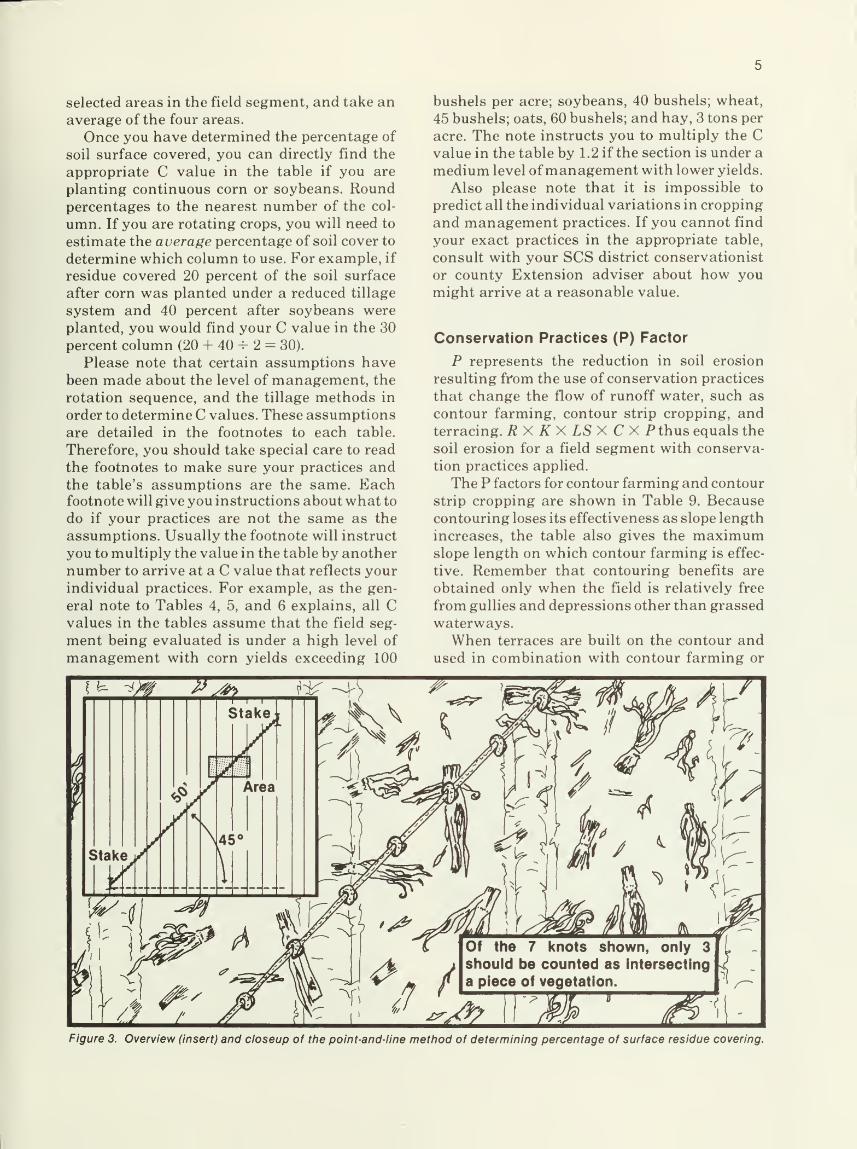
selected areas in the field segment, and take anaverage of the four areas.

Once you have determined the percentage of

soil surface covered, you can directly find the

appropriate C value in the table if you are

planting continuous corn or soybeans. Roundpercentages to the nearest number of the col-

umn. If you are rotating crops, you will need to

estimate the average percentage of soil cover to

determine which column to use. For example, if

residue covered 20 percent of the soil surface

after corn was planted under a reduced tillage

system and 40 percent after soybeans were

planted, you would find your C value in the 30

percent column (20 + 40 ^ 2 = 30).

Please note that certain assumptions havebeen made about the level of management, the

rotation sequence, and the tillage methods in

order to determine C values. These assumptionsare detailed in the footnotes to each table.

Therefore, you should take special care to read

the footnotes to make sure your practices andthe table's assumptions are the same. Eachfootnote will give you instructions about what to

do if your practices are not the same as the

assumptions. Usually the footnote will instruct

you to multiply the value in the table by another

number to arrive at a C value that reflects yourindividual practices. For example, as the gen-

eral note to Tables 4, 5, and 6 explains, all Cvalues in the tables assume that the field seg-

ment being evaluated is under a high level of

management with corn yields exceeding 100

bushels per acre; soybeans, 40 bushels; wheat,

45 bushels; oats, 60 bushels; and hay, 3 tons per

acre. The note instructs you to multiply the Cvalue in the table by 1.2 if the section is under a

medium level ofmanagement with lower yields.

Also please note that it is impossible to

predict all the individual variations in cropping

and management practices. If you cannot find

your exact practices in the appropriate table,

consult with your SCS district conservationist

or county Extension adviser about how youmight arrive at a reasonable value.

Conservation Practices (P) Factor

P represents the reduction in soil erosion

resulting from the use of conservation practices

that change the flow of runoff water, such as

contour farming, contour strip cropping, andterracing. RxKXLSXCX Pthus equals the

soil erosion for a field segment with conserva-

tion practices applied.

The P factors for contour farming and contour

strip cropping are shown in Table 9. Because

contouring loses its effectiveness as slope length

increases, the table also gives the maximumslope length on which contour farming is effec-

tive. Remember that contouring benefits are

obtained only when the field is relatively free

from gullies and depressions other than grassed

waterways.

When terraces are built on the contour andused in combination with contour farming or

Figure 3. Overview (insert) and closeup of the point-and-line method of determining percentage of surface residue covering.

contour strip cropping, you must use Tables 9

and 10 in conjunction to determine your P value.

(P values are not used when terraces are not

built on the contour. Parallel terrace systems

may not meet the contour criteria.) After choos-

ing values from both tables, you multiply these

values to arrive at the correct P value.

For example, assume that you have installed

level ridge tile outlet terraces on the contour, 120

feet apart, on a 5 percent slope, and contour

farmed. From Table 9 you would determine that

the contour factor is 0.5, while from Table 10

you would determine that the terrace factor is

0.6. You would then multiply the two factors to

arrive at a conservation practices (P) value of

0.3 (0.5 X 0.6 = 0.3). This is the value that youwould insert into the USLE to determine the

annual soil erosion rate.

Research has shown that trapped sediment

accumulates in the terrace channel and ridge

area to such an extent that this portion of the

land does not deteriorate significantly. The Pfactor is proportioned to give credit where the

soil resource is maintained, that is, the factor

gets larger as the terrace interval gets wider,

thus giving less credit. Tile outlet terraces are

more effective in trapping sediment than openoutlets, and trapping efficiency goes down as

terrace grade increases.

Using the USLEWorking through Some Examples

How the land's physical features, the climate,

your crops, and your soil conservation practices

affect soil losses has been briefly discussed. TheUSLE enables you to estimate your averageannual soil erosion losses for a cropping andmanagement system by multiplying all the

values assigned to factors that affect erosion.

Two examples ofhow to use the equation follow.

Example 1. Our first example assumes a farmin Pike County, Illinois, with Fayette silt-loam

soil. The field segment is on a 5 percent slope

that is 300 feet long. The R value for Pike Countyis 200 (Figure 1); the K value for Fayette silt-

loam is 0.37 (Table 1); the LS value is 0.93 (Table

3). The amount of soil lost annually under fallow

would thus be:

R K LS A200 X 0.37 X 0.93 = 68.8 tons

Figure 2 indicates that the C values for Pike

County can be found in Table 5. The crop

rotation used is corn, soybeans, wheat, and a

clover catch crop. The field is conventionally

tilled and spring plowed. Residues are left on the

soil surface, and soybeans are drilled in 10-inch

rows. The field segment is under a high level of

management. According to Table 5, therefore,

the C factor is 0.22. (Note that footnote / indi-

cates to use the same C factor with or without

legume seeding.) We can now determine the

annual soil erosion loss that would occur if the

farm did not use conservation practices (P value):

C AR X K X LS = 68.8 X 0.22 = 15 tons

If the field is contour farmed, a P factor of 0.5

(Table 9) would be multiplied by the above value

to determine A. As a result, the amount of soil

lost annually would be:

P AR X K X LS X C = 15 X 0.5 = 7.6 tons

Because the soil loss tolerance level is 5 tons

per acre for a Fayette silt-loam soil that hasmore than three inches of topsoil (Table 1), 7.6

tons per acre is well above the limit.

Ifthe tillage system were changed to a reduced

tillage system that used primary tillage and twosecondary operations prior to planting, A wouldbe significantly lower. Let us assume that this

reduced tillage system resulted in an average

percentage of soil cover of 40 percent (the aver-

age of the percent residue cover after corn wasplanted and after soybeans were planted). The Cvalue, according to Table 5, would change to

0.12. As a result, A would reduce to:

R K LS C P A200 X 0.37 X 0.93 X 0.12 X 0.5 = 4.1 tons

Thus, this particular cropping and manage-ment system would bring the average annualsoil erosion below the 5-ton soil erosion limit.

Other conservation options include terracing

the field, changing the crop rotation, using zero

till, or using a combination of practices.

Example 2, As a second example, let us assumea farm in Perry County with a field segment of

Ava silt loam soil and a 5 percent slope that is

200 feet long. The R value for Perry County is

220 (Figure 1); the K value for silt loam is 0.43

(Table 1); the LS value is 0.76 (Table 3). The Tvalue for this soil is 4 tons per acre (Table 1). Thecalculation below gives the annual soil loss

under fallow:

R K LS220 X 0.43 X 0.76

A71.9 tons

Figure 2 indicates that the C value for Perry

County can be found in Table 6. On this seg-

ment, a corn and soybean rotation is grownconventionally tilled and spring plowed. Bothcrops are planted in 30-inch rows. The field

segment is under a medium level of manage-ment with corn yields of 75 bushels per acre andsoybean yields of 33 bushels per acre.

According to the spring plow column in Table

6, therefore, the C value is 0.31. However, the

general note to the entire table indicates that the

value in the table must be multiplied by 1.2

when the field is under a medium level of

management. The C value for the field segmentin this example is thus actually 0.37 (0.31 X 1.2).

As a result, 26.6 tons of soil would be lost

annually without any conservation practices:

C AR X K X LS = 71.9 X 0.37 = 26.6 tons

If the field is contour plowed, a P factor of 0.5

(Table 9) would be multiplied by the above value

to determine A under conservation practices:

P A26.6 X 0.5 = 13.3 tons

This value is substantially above the T value of

4. The farmer would thus probably have to

change several practices to lower the value.

Perhaps the operator would consider chang-

ing to a no-till system. But would such a changelower the soil loss to the established T value? Aquick answer can be obtained by looking at the

C value for a no-till corn-soybean rotation.

Assuming that such a no-till rotation wouldachieve an average of 50 percent soil cover after

planting, the C value would be 0.11. However, if

the operator still plans a medium level of man-agement, the C value actually would be 0.13

(0.11 X 1.2). As the calculation below indicates,

a no-till system would substantially reduce the

field's annual soil loss, nearly meeting the Tvalue and long-term state goals:


Increasing the crop yield to meet the high level

of management would lower the soil loss to

below the T value:


Of course, other options exist. The operator

could change the rotation (corn and double-crop,

no-till wheat and soybeans, for example, wouldresult in a C value of 0.08), use a combination

tillage system, terrace on the contour, or plant

narrow-row soybeans, to name a few.

As both these examples suggest, the use of the

USLE is not just limited to determining the

nearness of your soil loss to the T value. TheUSLE also can be used to evaluate the effects of

your management decisions on the soil erosion

on your farm.

Solving the USLE for C

Let us assume that you have determined yourannual rate of soil loss using the USLE andfound that the rate is above the T value for your

soil type. If you do not have the option of

changing or adding conservation practices (P

value), you will want to know what particular

cropping and management practices (C value)

would lower your annual rate to or below the Tvalue. To solve the USLE for C, use the follow-

ing formula:

R X K X LS X P

Using the information from Example 1, wecould solve for an acceptable C factor:

5 5

200 X 0.37 X 0.93 X 0.5 34.4= 0.14

After solving this equation, we would knowthat any crop rotation and tillage system in

Table 5 with a Cfactorof 0.14 or less would help

us meet the annual soil erosion goal in that

example of 5 tons per acre.

Getting Help

The Soil Conservation Service (SCS) district

conservationist located in each of the soil andwater conservation district offices has for manyyears used this method of estimating soil ero-

sion losses. Therefore, you may wish to have anSCS representative assist you in determining

the appropriate factors to insert into the USLE.The district conservationist can also help you

by recommending alternative soil erosion con-

trol practices. In addition, the SCS conserva-

tionist can supply you with C values for com-

binations of tillage systems for a rotation.

8

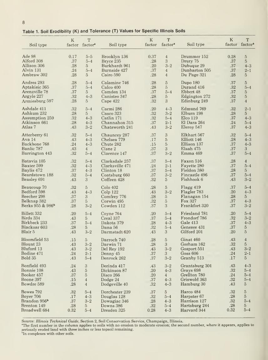
Table 1. Soil Erodlbllity (K) and Tolerance (T) Values for Specific Illinois Soils

K T K T K TSoil type factor factor* Soil type factor factor* Soil type factor factor*

Ade98 0.17 5-5 Brooklyn 136 0.37 4 Drummer 152 0.28 5Alford 308 .37 5-4 Bryce 235 .28 3 Drury 75 .37 5

Allison 306 .28 5 Burkhardt 961 .20 3-2 Dubuque 29 .37 4-3

Alvin 131 .24 5-4 Burnside 427 .37 4 Dunbarton 505 .37 2-1

Ambraw 302 .28 5 Cairo 590 .28 4 Du Page 321 .28 5

Andres 293 .28 5-4 Calamine 746 .28 5 Dupo 180 .37 5Aptakisic 365 .37 5-4 Calco 400 .28 5 Durand 416 .32 5-4

Arenzville 78 .37 5 Camden 134 .37 5-4 Ebbert 48 .37 5Argyle 227 .32 4-3 Canisteo 347 .28 5 Edgington 272 .32 5

Armiesburg 597 .28 5 Cape 422 .32 3 Edinburg 249 .37 4

Ashdale411 .32 5-4 Carmi 286 .20 4-3 Edmund 769 .32 2-1

Ashkum 232 .28 5 Casco 323 .32 3-2 Elburn 198 .28 5

Assumption 259 .32 4-3 Catlin 171 .32 5-4 Elcoll9 .37 4-3

Atkinson 661 .28 4-3 Channahon 315 .37 2-1 El Dara 264 .24 5-4

Atlas 7 .43 3-2 Chatsworth 241 .43 3-2 Eleroy 547 .37 4-3

Atterberry 61 .32 5-4 Chauncey 287 .37 3 Elkhart 567 .32 5-4

Ava 14 .43 4-3 Chelsea 779 .17 5 ElHott 146 .28 4-3

Backbone 768 .24 4-3 Chute 282 .15 5 ElHson 137 .37 4-3

Banlic 787 .43 4 Cisne 2 .37 3 Elsah 475 .37 3

Harrington 443 .32 5-4 Clarence 147 .37 3-2 Emma 469 .37 5-4

Batavia 105 .32 5-4 Clarksdale 257 .37 5-4 Faxon 516 .28 4

Baxter 599 .32 4-3 Clarksville 471 .24 2-1 Fayette 280 .37 5-4

Baylis 472 .37 4-3 CHnton 18 .37 5-4 Fieldon 380 .28 5

Beardstown 188 .32 5-4 Coatsburg 660 .37 3-2 Fincastle 496 .37 5-4

Beasley 691 .43 3 Coffeen 428 .32 5 Fishhook 6 .43 3-2

Beaucoup 70 .32 5 Colo 402 .28 5 Flagg 419 .37 5-4

Bedford 598 .43 4-3 Colp 122 .43 3-2 Flagler 783 .20 4-3

Beecher 298 .37 3 Comfrey 776 .28 5 Flanagan 154 .28 5

Belknap 382 .37 5 Corwin 495 .32 5 Fox 327 .37 4-3

Berks 955 & 986" .28 3-2 Cowden 112 .37 3 Frankfort 320 .37 3-2

Billett 332 .20 5-4 Coyne 764 .20 5-4 Friesland 781 .20 5-4

Birds 334 .43 5 Creal 337 .37 5-4 Frondorf 786 .32 3-2

Birkbeck 233 .37 5-4 Dakota 379 .28 4-3 Gale 413 .37 4-3

Blackoar 603 .28 5 Dana 56 .32 5-4 Genesee 431 .37 5

Blair 5 .43 3-2 Darmstadt 620 .43 3 Gilford 201 .20 5

Bloomfield 53 .15 5 Darroch 740 .28 5 Ginat 460 .43 4

Blount 23 .43 3-2 Darwin 71 .28 3 Gorham 162 .32 5

Bluford 13 .43 3-2 Del Rey 192 .43 3-2 Gosport 551 .43 3-2

Bodine 471 .24 2-1 Denny 45 .37 3 Goss 606 .24 2-1

Bold 35 .43 5-4 Denrock 262 .37 3-2 Granby 513 .17 5

Bonfield 493 .24 3 Derinda 417 .43 3-2 Grantsburg 301 .43 4-3

Bonnie 108 .43 5 Dickinson 87 .20 4-3 Grays 698 .32 5-4

Booker 457 .37 5 Disco 266 .20 4 Grellton 780 .24 5-4

Boone 397 .15 4 Dodge 24 .37 4-3 Griswold 363 .32 5-4

Bowdre 589 .28 4 Dodgeville 40 .32 4-3 Hamburg 30 .43 5

Bowes 792 .32 5-4 Dorchester 239 .37 5 Harco 484 .32 5

Boyer 706 .17 4-3 Douglas 128 .32 5-4 Harpster 67 .28 5

Brandon 956" .37 3-2 Dowagiac 346 .28 4-3 Harrison 127 .32 5-4

Brenton 149 .28 5 Downs 386 .32 5-4 Hartsburg 244 .28 5

Broadwell 684 0.32 5-4 Dresden 325 0.28 4-3 Harvard 344 0.32 5-4

Source: Illinois Technical Guide, Section 2, Soil Conservation Service, Champaign, Illinois.

^The first number in the column applies to soils with no erosion to moderate erosion; the second number, where it appears, applies to

seriously eroded land with three inches or less topsoil remaining.

''In complexes with other soils.

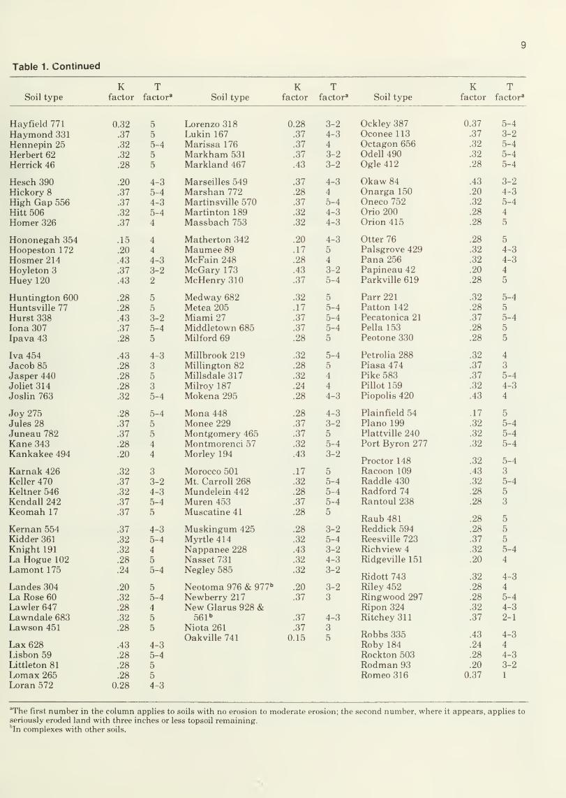
Table 1. Continued

K T K T K TSoil type factor factor^ Soil type factor factor' Soil type factor factor'

Hayfield 771 0.32 5 Lorenzo 318 0.28 3-2 Ockley 387 0.37 5-4

Haymond 331 .37 5 Lukin 167 .37 4-3 Oconee 113 .37 3-2

Hennepin 25 .32 5-4 Marissa 176 .37 4 Octagon 656 .32 5-4

Herbert 62 .32 5 Markham 531 .37 3-2 Odell 490 .32 5-4

Herrick 46 .28 5 Markland 467 .43 3-2 Ogle 412 .28 5-4

Hesch 390 .20 4-3 Marseilles 549 .37 4-3 Okaw 84 .43 3-2

Hickory 8 .37 5-4 Marshan 772 .28 4 Onarga 150 .20 4-3

High Gap 556 .37 4-3 Martinsville 570 .37 5-4 Oneco 752 .32 5-4

Hitt 506 .32 5-4 Martinton 189 .32 4-3 Orio 200 .28 4

Homer 326 .37 4 Massbach 753 .32 4-3 Orion 415 .28 5

Hononegah 354 .15 4 Matherton 342 .20 4-3 Otter 76 .28 5

Hoopeston 172 .20 4 Maumee 89 .17 5 Palsgrove 429 .32 4-3

Hosmer 214 .43 4-3 McFain 248 .28 4 Pana 256 .32 4-3

Hoyleton 3 .37 3-2 McGary 173 .43 3-2 Papineau 42 .20 4

Huey 120 .43 2 McHenry 310 .37 5-4 Parkville 619 .28 5

Huntington 600 .28 5 Medway 682 .32 5 Parr 221 .32 5-4

Huntsville 77 .28 5 Metea 205 .17 5-4 Patton 142 .28 5

Hurst 338 .43 3-2 Miami 27 .37 5-4 Pecatonica 21 .37 5-4

lona 307 .37 5-4 Middletown 685 .37 5-4 Pella 153 .28 5

Ipava 43 .28 5 Milford 69 .28 5 Peotone 330 .28 5

Iva 454 .43 4-3 Millbrook 219 .32 5-4 Petrolia 288 .32 4

Jacob 85 .28 3 Millington 82 .28 5 Piasa 474 .37 3

Jasper 440 .28 5 Millsdale317 .32 4 Pike 583 .37 5-4

Joliet 314 .28 3 Milroy 187 .24 4 Pillot 159 .32 4-3

Joslin 763 .32 5-4 Mokena 295 .28 4-3 Piopolis 420 .43 4

Joy 275 .28 5-4 Mona 448 .28 4-3 Plainfield 54 .17 5

Jules 28 .37 5 Monee 229 .37 3-2 Piano 199 .32 5-4

Juneau 782 .37 5 Montgomery 465 .37 5 Plattville 240 .32 5-4

Kane 343 .28 4 Montmorenci 57 .32 5-4 Port Byron 277 .32 5-4

Kankakee 494 .20 4 Morley 194 .43 3-2Proctor 148 .32 5-4

Karnak 426 .32 3 Morocco 501 .17 5 Racoon 109 .43 3

Keller 470 .37 3-2 Mt. Carroll 268 .32 5-4 Raddle 430 .32 5-4

Keltner 546 .32 4-3 Mundelein 442 .28 5-4 Radford 74 .28 5

Kendall 242 .37 5-4 Muren 453 .37 5-4 Rantoul 238 .28 3

Keomah 17 .37 5 Muscatine 41 .28 5Raub 481 .28 5

Kernan 554 .37 4-3 Muskingum 425 .28 3-2 Reddick 594 .28 5

Kidder 361 .32 5-4 Myrtle 414 .32 5-4 Reesville 723 .37 5

Knight 191 .32 4 Nappanee 228 .43 3-2 Richview 4 .32 5-4

La Hogue 102 .28 5 Nasset 731 .32 4-3 Ridgeville 151 .20 4

Lamont 175 .24 5-4 Negley 585 .32 3-2Ridott 743 .32 4-3

Landes 304 .20 5 Neotoma 976 & 977" .20 3-2 Riley 452 .28 4

La Rose 60 .32 5-4 Newberry 217 .37 3 Ringwood 297 .28 5-4

Lawler 647 .28 4 New Glarus 928 & Ripon 324 .32 4-3

Lawndale 683 .32 5 561" .37 4-3 Ritchey 311 .37 2-1

Lawson 451

Lax 628

.28

.43

5

4-3

Niota 261

Oakville 741

.37

0.15

3

5 Robbs 335Roby 184

.43

.24

4-3

4

Lisbon 59 .28 5-4 Rockton 503 .28 4-3

Littleton 81 .28 5 Rodman 93 .20 3-2

Lomax 265 .28 5 Romeo 316 0.37 1

Loran 572 0.28 4-3

""The first number in the column applies to soils with no erosion to moderate erosion; the second number, where it appears, applies to

seriously eroded land with three inches or less topsoil remaining.''In complexes with other soils.

10

Table 1. Continued

K T K T K TSoil type factor factor" Soil type factor factor' Soil type factor factor"

Ross 73 0.32 5 Strawn 224 0.37 4-3 Washtenaw 296 0.37 5

Rowe 230 .28 5 Streator 435 .28 3 Watseka 49 .17 2

Rozetta 279 .37 5-4 Stronghurst 278 .37 5-4 Wauconda 697 .32 4-3

Ruark 178 .24 4 Sunbury 234 .32 5-4 Waukee 727 .24 4-3

Rush 791 .37 5-4 Swygert 91 .43 3-2 Waukegan 564 .32 4-3

Rushville 16 .43 3 Sylvan 19 .37 5-4 Waupecan 369 .32 4-3

Russell 322 .37 5-4 Symerton 294 .32 5-4 Wea 398 .32 5-4

Rutland 375 .32 5-4 Tallula 34 .32 5-4 Weinbach 461 .43 4-3

Sabina 236 .37 5-4 Tama 36 .32 5-4 Weir 165 .43 4

Sable 68 .28 5 Tamalco 581 .43 3-2 Wellston 339 .37 4-3

Saffell 956" .20 4 Tell 565 .37 4-3 Wenona 388 .32 4-3

Sarpy 92 .15 5 Terril 587 .24 5 Wesley 141 .24 3-2

Saude 774 .28 4-3 Thebes 212 .37 4-3 Westland 300 .28 5

Sawmill 107 .28 5 Thorp 206 .37 4 Westmore 940" .37 4

Saybrook 145 .32 5-4 Tice 284 .32 4 Westville 22 .37 5-4

Saylesville 370 .37 3-2 Timula 271 .37 5-4 Whalan 509 .32 4-3

Schapville 418 .32 3-2 Titus 404 .32 4 WheeHng 463 .32 4-3

Sciotoville 462 .37 4-3 Toronto 353 .32 5-4 Whitson 116 .43 4

Seaton 274 .37 5-4 Traer 633 .37 5 Will 329 .28 4

Selma 125 .28 5 Trempealeau 765 .28 3 Wingate 348 .32 5-4

Sexton 208 .43 4 Troxel 197 .28 5 Winnebago 728 .32 5-4

Shadeland 555 .37 4 Uniontown 482 .37 4-3 Woodbine 410 .37 4-3

Sharon 72 .37 5 Ursa 605 .37 4-3 Worthen 37 .32 5-4

Shiloh 138 .28 3 Varna 223 .32 4-3 Wynoose 12 .43 3

Shoals 424 .37 5 Velma 250 .32 4-3 Xenia 291 .37 5-4

Shullsburg 745 .32 4-3 Virden 50 .28 5 Zanesville 340 .43 3-2

Sidell 55 .32 5-4 Virgil 104 .32 5-4 Zipp 524 .28 5

Sogn 504 .28 1 Wabash 83 .28 5 Zurich 696 .37 5-4

Sparta 88 .17 5 Wagner 26 .28 3 Zwingle 576 0.43 3-2

St. Charles 243 .37 5-4Wakeland 333 .37 5

St. Clair 560 .37 3-2 Walshville 584 .43 3-2

Starks 132 .37 5 Ware 456 .32 4

Stockland 155 .20 2-1 Warsaw 290 .28 4-3

Stonelick 665 .24 5 Wartrace 215 0.37 5-4

Stoy 164 0.43 4-3

"The first number in the column applies to soils with no erosion to moderate erosion; the second number, where it appears, applies toseriously eroded land with three inches or less topsoil remaining.In complexes with other soils.

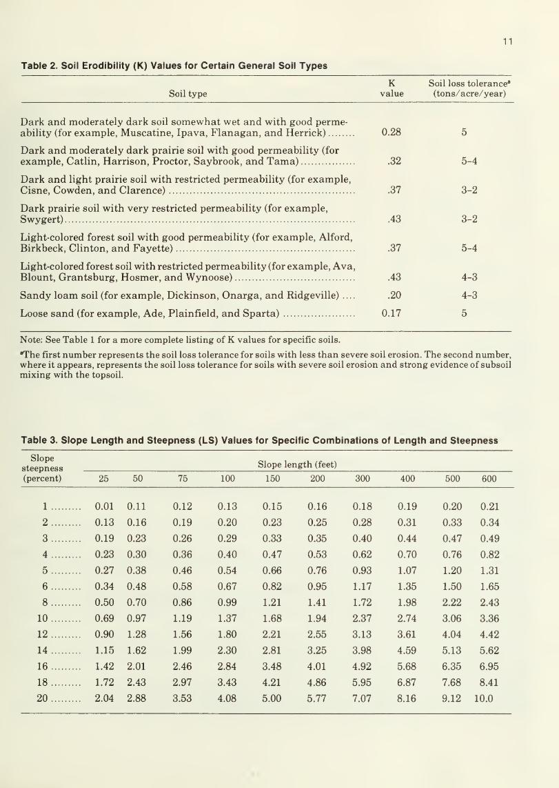
Table 2. Soil Erodlbility (K) Values for Certain General Soil Types

11

Soil type

K Soil loss tolerance"

value (tons/acre/year)

Dark and moderately dark soil somewhat wet and with good perme-ability (for example, Muscatine, Ipava, Flanagan, and Herrick) 0.28 5

Dark and moderately dark prairie soil with good permeability (for

example, Catlin, Harrison, Proctor, Saybrook, and Tama) .32 5-4

Dark and light prairie soil with restricted permeability (for example,Cisne, Cowden, and Clarence) .37 3-2

Dark prairie soil with very restricted permeability (for example,Swygert) .43 3-2

Light-colored forest soil with good permeability (for example, Alford,

Birkbeck, Clinton, and Fayette) .37 5-4

Light-colored forest soil with restricted permeability (for example, Ava,Blount, Grantsburg, Hosmer, and Wynoose) .43 4-3

Sandy loam soil (for example, Dickinson, Onarga, and Ridgeville) .... .20 4-3

Loose sand (for example, Ade, Plainfield, and Sparta) 0.17 5

Note: See Table 1 for a more complete listing of K values for specific soils.

"The first number represents the soil loss tolerance for soils with less than severe soil erosion. The second number,where it appears, represents the soil loss tolerance for soils with severe soil erosion and strong evidence of subsoil

mixing with the topsoil.

Table 3. Slope Length and Steepness (LS) Values for Specific Combinations of Length and Steepness

Slopesteepness Slope length (feet)

(percent) 25 50 75 100 150 200 300 400 500 600

1 0.01 0.11 0.12 0.13 0.15 0.16 0.18 0.19 0.20 0.21

2 0.13 0.16 0.19 0.20 0.23 0.25 0.28 0.31 0.33 0.34

3 0.19 0.23 0.26 0.29 0.33 0.35 0.40 0.44 0.47 0.49

4 0.23 0.30 0.36 0.40 0.47 0.53 0.62 0.70 0.76 0.82

5 0.27 0.38 0.46 0.54 0.66 0.76 0.93 1.07 1.20 1.31

6 0.34 0.48 0.58 0.67 0.82 0.95 1.17 1.35 1.50 1.65

8 0.50 0.70 0.86 0.99 1.21 1.41 1.72 1.98 2.22 2.43

10 0.69 0.97 1.19 1.37 1.68 1.94 2.37 2.74 3.06 3.36

12 0.90 1.28 1.56 1.80 2.21 2.55 3.13 3.61 4.04 4.42

14 1.15 1.62 1.99 2.30 2.81 3.25 3.98 4.59 5.13 5.62

16 1.42 2.01 2.46 2.84 3.48 4.01 4.92 5.68 6.35 6.95

18 1.72 2.43 2.97 3.43 4.21 4.86 5.95 6.87 7.68 8.41

20 2.04 2.88 3.53 4.08 5.00 5.77 7.07 8.16 9.12 10.0

12

Table 4. Cropping and Management (C) Values for Northern Illinois

Soybeanrow

width"

Conventionaltillage*^

Chisel, disk

20% 30%

or ridge**®

40% 50%

All corn and soybeans planted no-till*Crop

sequence*Fallplow

Springplow 20% 30% 40% 50% 60% 70% 80% 90%

Continuoussoybeans wide

narrow.44

.36

.39

.32

.36

.31

.32

.29

.25 .20

.21 .18

.16

.15

Continuouscorn .34 .29 .21 .18 .15 .12 .08 .06 .04 .03

C-Sb wide .38 .33 .28 .24 .20 .19 .18 .14 .10 .09

narrow .34 .30 .27 .23 .19 .18 .17 .14 .10 .09

C-C-Sb wide .36 .32 .26 .22 .18 .17 .14 .11 .08 .07

narrow .34 .30 .25 .21 .17 .16 .14 .11 .08 .07

C-Sb-G' wide .27 .25 .18 .16 .13 .12 .10 .07 .05 .04

narrow .25 .23 .17 .15 .12 .11 .09 .07 .05 .04

C-C-G-M^*^ .14 .12 .10 .09 .08 .07 .04 .03 .02 .02

C-Sb-G-M9'' wide .15 .13 .10 .09 .08 .08 .05 .04 .03 .03

narrow .13 .12 .10 .09 .08 .07 .05 .04 .03 .03

C-Sb-M-Mfl-»' wide .12 .10 .08 .07 .06 .06 .03 .02 .02 .01

narrow .11 .08 .07 .07 .06 .06 .03 .02 .02 .01

C-G-M9*' .09 .07 .07 .07 .06 .06 .03 .02 .02 .01

C-M-M-Mfl*^ .05 .04 .01 .008 .006 .006

Combination Tillage Systems

Cropsequence'

C-Sb

Tillage systems used for sequence

Corn after soybeans, no-till; soybeans after corn,fall chisel, spring secondary tillage

Soybean rowwidth*'

wide

narrow

Percent soil cover afterplanting each crop

20%

.23

.21

30%

.19

.18

40%

.15

.14

Source: C values for this table were calculated from the Soil Conservation Service's Illinois Technical Guide, Section I-C (EI Curve 14).

NOTE: Values in this table are based on high level management with yields equal to or exceeding the following: corn, 100

bushels per acre; soybeans, 40 bushels per acre; wheat, 45 bushels per acre; oats, 60 bushels per acre; meadow, 3 tons per

acre. For medium level management, multiply values by 1.2.

*In this column, C = corn, Sb = soybeans, G ~ small grain, M = meadow, and W = wheat.

"Use the wide-row values for soybean rows wider than 20 inches. Use the narrow-row values for soybean rows planted 20inches or less, including drilled.

''Where corn residue is removed for silage or other purposes, multiply the C value by 1.2 for intensive rotations such as

corn and soybeans or corn, corn, and soybeans. Do not multiply the C value by any number for the less intensive

rotations, including meadow crops, where crop residue is removed.

"Values for chisel and disk systems are for aSi primary tillage and two secondary tillage operations prior to planting. Forprimary tillage in the spring or ridge planting up and down hill, multiply the appropriate C values by 0.9 in northern

Illinois, by 0.8 in central Illinois, and by 0.7 in southern Illinois. For ridge planting on the contour, multiply the

appropriate C value by 0.7 in northern Illinois, by 0.6 in central Illinois, and by 0.5 in southern Illinois. Ridge planting is

applicable only for row crops following row crops.

®The percent figures represent the percentage of the soil surface covered after planting. The percent figure for a rotation is

equal to the average cover for the crop sequence. For example, if, in a corn-soybean rotation, residue covered 20 percent of

the soil surface after corn was planted and 60 percent after soybeans were planted, the average cover would be 40 percent,

and you would find your C value in the 40 percent column.

The same C values are applicable for small grain both with and without a catch crop.

^Chisel and disk C values are calculated for spring-plow, conventional tillage when corn follows meadow.

''Values are based on a sod or grass legume mixture consisting of at least 50 percent grass and established at least one full

growing season. If meadow is primarily legume, multiply the appropriate C value by 1.2.

13

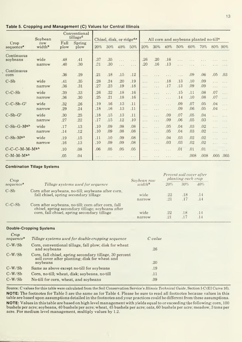
Table 5. Cropping and Management (C) Values for Central Illinois

Cropsequence"

Soybeanrow

width"


Fall Springplow plow

Chisel, disk, or ridge**'*

20% 30% 40% 50%

All corn and soybeans planted no-till'

20% 30% 40% 50% 60% 70% 80% 90%

Continuoussoybeans wide .48 .41

narrow .40 .30

Continuouscorn .36 .29

C-Sb wide .41 .35

narrow .36 .31

C-C-Sb wide .39 .33

narrow .36 .30

C-C-Sb-G' wide .32 .26

narrow .29 .24

C-Sb-G' wide .30 .25

narrow .27 .22

C-Sb-G-Mfl'*' wide .17 .13

narrow .14 .12

C-Sb-Mfl-*' wide .19 .15

narrow .16 .13

C-C-C-M-M-Ms-*^ .10 .08

C-M-M-Ma-"^ .05 .04

.37

.31

.21

.28

.27

.26

.25

.19

.18

.18

.17

.10

.10

.11

.10

.06

.35

.30

.18

.24

.23

.22

.21

.16

.16

.15

.15

.09

.09

.10

.09

.05

15

20

19

18

18

13

13

13

12

08

08

09

09

.12

.19

.18

.16

.16

.11

.11

.11

.10

.08

.08

.08

.08

05 .05

26

20

20

16

.16

.13

.18

.17

.09 .06 .05 03

.09

.09

.05

.05

.04

.03

.13

.13

.15

.14

.09

.09

.07

.06

.04

.04

.03

.03

.01

.10

.09

.11

.10

.07

.06

.05

.05

.03

.03

.02

.02

.09

.09

.08

.08

.05

.05

.04

.03

.02

.02

.02

.02

.07

.07

.04

.04

.01 .01

.008 .008 .005 .005


Cropsequence^

C-Sb

C-C-Sb



Corn after soybeans, no-till; corn after corn, fall

chisel, spring secondary tillage; soybeans aftercorn, fall chisel, spring secondary tillage

Soybean row


width" 20% 30% 40%)

widenarrow

.22

.21

.18

.17

.14

.14

widenarrow

.22

.21

.18

.17

.14

.14

Double-Cropping Systems

Cropsequence' Tillage systems used for double-cropping sequence

C-W/Sb Corn, conventional tillage, fall plow; disk for wheatand soybeans

C-W/Sb Corn, fall chisel, spring secondary tillage, 30 percentsoil cover after planting; disk for wheat andsoybeans

C-W/Sb Same as above except no-till for soybeans

C-W/Sb Corn, no-till; wheat, disk; soybeans, no-till

C-W/Sb No-till for corn, wheat, and soybeans

C value

.26

.20

.19

.11

.09


NOTE: The footnotes for Table 5 are the same as for Table 4. Please be sure to read all footnotes because values in this

table are based upon assumptions detailed in the footnotes and your practices could be different from these assumptions.

NOTE: Values in this table are based on high level management with yields equal to or exceeding the following: corn, 100bushels per acre; soybeans, 40 bushels per acre; wheat, 45 bushels per acre; oats, 60 bushels per acre; meadow, 3 tons peracre. For medium level management, multiply values by 1.2.

14

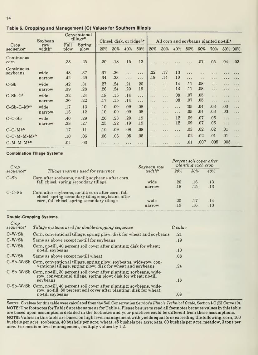
Table 6. Cropping and Management (C) Values for Southern Illinois

Soybeanrow

width"


Chise

20%

I, disk

30%

or ri

40%

dge"*-'

50%

All onvn nnH ssoybeans planted n o-till*

Cropsequence*

Fall Springplow plow

* *** w-.-.-. *^M.m.-»^ m.

20% 30% 40% 50% 60% 70% 80% 90%

Continuouscorn .38 .25 .20 .18 .15 .13 .07 .05 .04 .03

Continuoussoybeans wide

narrow.48 .37

.42 .29

.37

.34

.36

.33

.22 .17 .13

.19 .14 .10

C-Sb wide .42 .31 .27 .24 .21 .20 . .14 .11 .08

narrow .39 .28 .26 .24 .20 .19 .. .14 .11 .08

C-Sb-G' wide .32 .24 .18 .15 .14 .. .08 .07 .05

narrow .30 .22 .17 .15 .14 .. .08 .07 .05

C-Sb-G-M''** wide .17 .13 .10 .09 .09 .08 ... .05 .04 .03 .03

narrow .16 .12 .10 .09 .09 .08 .05 .04 .03 .03

C-C-Sb wide .40 .29 .26 .23 .20 .19 .. .12 .09 .07 .06 ...

narrow .38 .27 .25 .22 .19 .19 .. .12 .09 .07 .06

C-C-Mo" .17 .11 .10 .09 .08 .08 ... .03 .02 .02 .01

C-C-M-M-M8 h .10 .06 .06 .06 .05 .05 ... .02 .02 .01 .01

C-M-M-Mo-" .04 .03 .01 .007 .005 .005 .


Cropsequence'

C-Sb

C-C-Sb



Corn after soybeans, no-till; corn after corn, fall

chisel, spring secondary tillage; soybeans after

corn, fall chisel, spring secondary tillage

Soybean row


width" 20% 30% 40%

wide .20 .16 .13

narrow .18 .15 .13

wide .20 .17 .14

narrow .19 .16 .13

Double-Cropping Systems

Cropsequence' Tillage systems used for double-cropping sequence

C-W/Sb Corn, conventional tillage, spring plow; disk for wheat and soybeans

C-W/Sb Same as above except no-till for soybeans

C-W/Sb Corn, no-till, 40 percent soil cover after planting; disk for wheat;no-till soyl)eans

C-W/Sb Same as above except no-till wheat

C-Sb-W/Sb Com, conventional tillage, spring plow; soybeans, wide-row, con-ventional tillage, spring plow; disk for wheat and soybeans

C-Sb-W/Sb Corn, no-till, 30 percent soil cover after planting; soybeans, wide-row, conventional tillage, spring plow; disk for wheat; no-till

soybeans

C-Sb-W/Sb Corn, no-till, 40 percent soil cover after planting; soybeans, wide-row, no-till, 80 percent soil cover after planting; disk for wheat;no-till soybeans

C value

.21

.19

.10

.08

.24

.18

.08


NOTE: The footnotes for Table 6 are the same as for Table 4. Please be sure to read all footnotes because values in this table

are based upon assumptions detailed in the footnotes and your practices could be different from these assumptions.

NOTE: Values in this table are based on high level management with yields equal to or exceeding the following: corn, 100

bushels per acre; soybeans, 40 bushels per acre; wheat, 45 bushels per acre; oats, 60 bushels per acre; meadow, 3 tons per

acre. For medium level management, multiply values by 1.2.

15

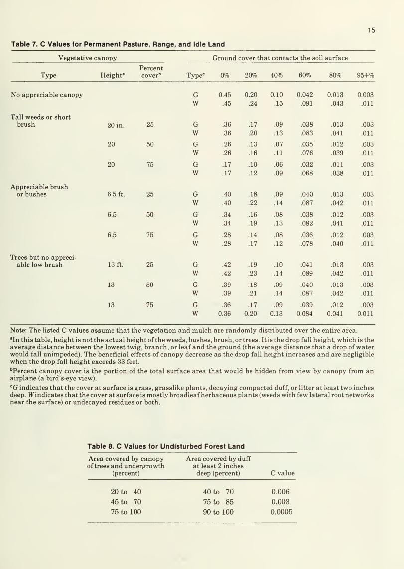
Table 7. C Values for Permanent Pasture, Range, and Idle Land

Vegetative canopy Ground cover that contacts the soil surface

Type Height"Percentcover" Type' 0% 20% 40% 60% 80% 95+%

No appreciable canopy G 0.45 0.20 0.10 0.042 0.013 0.003

W .45 .24 .15 .091 .043 .011

Tall weeds or shortbrush 20 in. 25 G .36 .17 .09 .038 .013 .003

W .36 .20 .13 .083 .041 .011

20 50 G .26 .13 .07 .035 .012 .003

W .26 .16 .11 .076 .039 .011

20 75 G .17 .10 .06 .032 .011 .003

W .17 .12 .09 .068 .038 .011

Appreciable brushor bushes 6.5 ft. 25 G .40 .18 .09 .040 .013 .003

W .40 .22 .14 .087 .042 .011

6.5 50 G .34 .16 .08 .038 .012 .003

W .34 .19 .13 .082 .041 .011

6.5 75 G .28 .14 .08 .036 .012 .003

W .28 .17 .12 .078 .040 .011

Trees but no appreci-

able low brush 13 ft. 25 G .42 .19 .10 .041 .013 .003

W .42 .23 .14 .089 .042 .011

13 50 G .39 .18 .09 .040 .013 .003

W .39 .21 .14 .087 .042 .011

13 75 G .36 .17 .09 .039 .012 .003

W 0.36 0.20 0.13 0.084 0.041 0.011

Note: The listed C values assume that the vegetation and mulch are randomly distributed over the entire area.

In this table, height is not the actual height ofthe weeds, bushes, brush, or trees. It is the drop fall height, which is theaverage distance between the lowest twig, branch, or leaf and the ground (the average distance that a drop of waterwould fall unimpeded). The beneficial effects of canopy decrease as the drop fall height increases and are negligible

when the drop fall height exceeds 33 feet.

''Percent canopy cover is the portion of the total surface area that would be hidden from view by canopy from anairplane (a bird's-eye view).

•^G indicates that the cover at surface is grass, grasslike plants, decaying compacted duff, or litter at least two inchesdeep. Wîndicates that the cover at surface is mostly broadleafherbaceous plants (weeds with few lateral root networksnear the surface) or undecayed residues or both.

Table 8. C Values for Undisturbed Forest Land

Area covered by canopyof trees and undergrowth

(percent)

Area covered by duff

at least 2 inchesdeep (percent) C value

20 to 40

45 to 70

75 to 100

40 to 70 0.006

75 to 85 0.003

90 to 100 0.0005

16

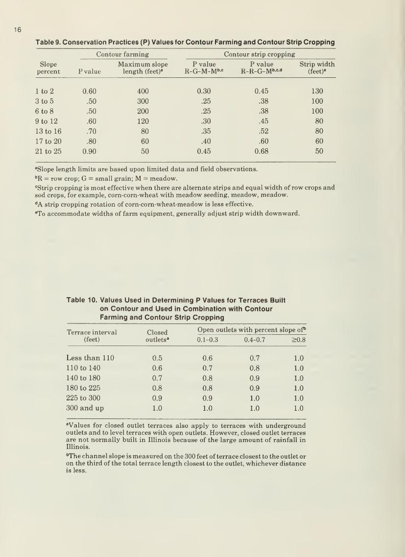
Table 9. Conservation Practices (P) Values for Contour Farming and Contour Strip Cropping

Contour farming Contour strip cropping

Slopepercent P value

Maximum slope

length (feet)"

P valueR-G-M-M"'

P valueR-R-G-M'''=''

Strip width(feet)«

lto2 0.60 400 0.30 0.45 130

3 to 5 .50 300 .25 .38 100

6 to 8 .50 200 .25 .38 100

9 to 12 .60 120 .30 .45 80

13 to 16 .70 80 .35 .52 80

17 to 20 .80 60 .40 .60 60

21 to 25 0.90 50 0.45 0.68 50

"Slope length limits are based upon limited data and field observations.

''R = row crop; G = small grain; M = meadow.

*^Strip cropping is most effective when there are alternate strips and equal width of row crops andsod crops, for example, corn-corn-wheat with meadow seeding, meadow, meadow.

**A strip cropping rotation of corn-corn-wheat-meadow is less effective.

*To accommodate widths of farm equipment, generally adjust strip width downward.

Table 10. Values Used in Determining P Values for Terraces Built

on Contour and Used in Combination with ContourFarming and Contour Strip Cropping

Terrace interval Closed Open outlets with percent slope of

(feet) outlets" 0.1-0.3 0.4-0.7 >0.8

Less than 110 0.5 0.6 0.7 1.0

110 to 140 0.6 0.7 0.8 1.0

140 to 180 0.7 0.8 0.9 1.0

180 to 225 0.8 0.8 0.9 1.0

225 to 300 0.9 0.9 1.0 1.0

300 and up 1.0 1.0 1.0 1.0

Values for closed outlet terraces also apply to terraces with undergroundoutlets and to level terraces with open outlets. However, closed outlet terracesare not normally built in Illinois because of the large amount of rainfall in

Illinois.

The channel slope is measured on the 300 feet of terrace closest to the outlet oron the third of the total terrace length closest to the outlet, whichever distanceis less.

17

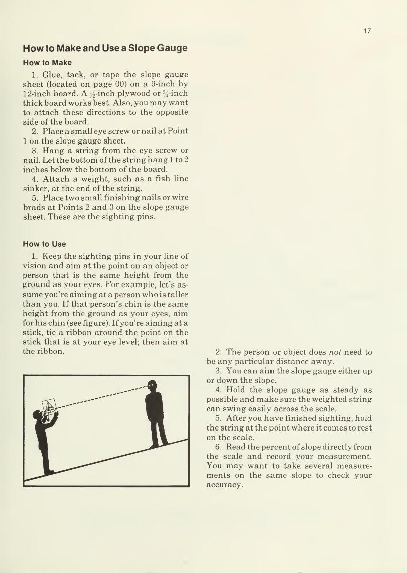
How to Make and Use a Slope Gauge

How to Make

1. Glue, tack, or tape the slope gauge

sheet (located on page 00) on a 9-inch by12-inch board. A V,-inch plywood or %-inch

thick board works best. Also, you may wantto attach these directions to the opposite

side of the board.

2. Place a small eye screw or nail at Point

1 on the slope gauge sheet.

3. Hang a string from the eye screw or

nail. Let the bottom of the string hang 1 to 2

inches below the bottom of the board.

4. Attach a weight, such as a fish line

sinker, at the end of the string.

5. Place two small finishing nails or wire

brads at Points 2 and 3 on the slope gaugesheet. These are the sighting pins.

How to Use

1. Keep the sighting pins in your line of

vision and aim at the point on an object or

person that is the same height from the

ground as your eyes. For example, let's as-

sume you're aiming at a person who is taller

than you. If that person's chin is the sameheight from the ground as your eyes, aimfor his chin (see figure). If you're aiming at a

stick, tie a ribbon around the point on the

stick that is at your eye level; then aim at

the ribbon. 2. The person or object does not need to

be any particular distance away.3. You can aim the slope gauge either up

or down the slope.

4. Hold the slope gauge as steady as

possible and make sure the weighted string

can swing easily across the scale.

5. After you have finished sighting, hold

the string at the point where it comes to rest

on the scale.

6. Read the percent of slope directly fromthe scale and record your measurement.You may want to take several measure-ments on the same slope to check youraccuracy.

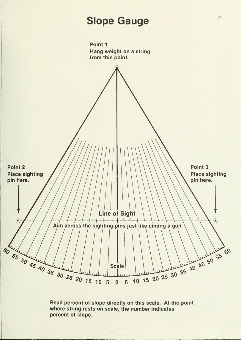
Slope Gauge 19

Point 1

Hang weight on a string

from this point.

Point 2

Place sighting

pin here.

^0

^03S

Point 3

Place sighting

pin here.

Aim

«>^

tf)

'' '' 20 IS 10 5 5 10 15 20 25 30

Read percent of slope directly on this scale. At the point

where string rests on scale, the number indicates

percent of slope.

35^

^84i1lll

Urbana, Illinois November, 1983

Issued in furtherance of Cooperative Extension Work, Acts of May 8 and June 30, 1914, in cooperation with the U.S.

Department of Agriculture, DONALD L. UCHTMANN, Director, Cooperative Extension Service, University of Illinois at

Urbana-Champaign. The Illinois Cooperative Extension Service provides equal opportunities in programs and employment.

1 .5M—Rep.— 1 2-93—MO

II ::»:

Documents

Estimating your soil erosion losses with the universal soil loss