Embed Size (px)
Citation preview
Revista Mexicana de Ciencias Agrícolas volume 9 number 6 August 14 - September 27, 2018
1109
Article
Analytical expressions of soil erosion and impact on their productivity
Ignacio Sánchez Cohen1
Aurelio Pedroza Sandoval2§
Miguel A. Velásquez Valle3
Palmira Bueno Hurtado1
Gerardo Esquivel Arriaga1
1INIFAP-National Center for Disciplinary Research in Water-Soil-Plant-Atmosphere Relationship. Right
bank channel Sacramento km 6.5, Gómez Palacio industrial zone, Durango. CP. 35140. Tel. 01(871)
1590105. 2Autonomous University Chapingo-Regional University Unit of Arid Zones. Dom. Acquaintance,
Bermejillo, Durango. Tel. 01(872) 7760160. 3INIFAP-Northeast Regional Research Center. Experimental
Field Saltillo. Carretera Saltillo-Zacatecas km 342 + 119, num. 9515, Hacienda de Buena Vista, Saltillo,
Coahuila. CP. 25315. Tel. 01(55) 38718700.
§Corresponding author: [email protected].
Abstract
The approximations for the estimation and projection of soil loss in hydrological basins, vary from
the empirical equations, to the use of models based on environmental physics. The objective of this
study was to generate and propose the use of a logistic differential equation for estimating soil loss.
By using an exponential model under conditions of soil deterioration, the yield loss of the corn
crop was estimated at 3.5 t ha-1, going from 4.5 to 1 t ha-1. The erosion model was parameterized
with information from an experimental INIFAP basin located in the municipality of San Luis of
Cordero, Durango. The results indicate that the average annual rate of soil loss is 0.44 mm year-1,
for which it was considered a critical rate of soil loss of 10 mm year-1. With that initial rate, the
range would reach its maximum allowable rate in 19 years. This study analyzes the behavior of the
model parameters from where other soil loss scenarios were tested where the maximum permissible
rate is reached at different times.
Keywords: environmental impact, process modeling, soil loss, yield.
Reception date: May 2018
Acceptance date: June 2018
Rev. Mex. Cienc. Agríc. vol. 9 num. 6 August 14 - September 27, 2018
1110
Introduction
Soil losses in watersheds is a recurring problem in hydrological studies faced by natural resource
users and the researchers themselves. These losses have effects in situ and ex situ of the affected
basins. In situ problems include the loss of soil structure, the decrease of soil organic matter and
nutrients, and the reduction of water availability in the soil (Brooks et al., 2012). Ex situ effects
increase the transport of sediments and the loss of nutrients such as nitrogen and phosphorus that
are adhered to eroded soil particles deposited in the drainage network of the basins, below where
the problem arises.
The increase of sediment in the drainage network of the basins reduces the transport capacity and
reduces the quality of the water that drains downstream where it is used for different uses (Ffolliot
et al., 2013). Also, the loss of soil due to water erosion is the main factor that limits the productivity
of soils that obstructs full production in agriculture (Obalum et al., 2012). Population growth and
change in land use exacerbate the process along with high rainfall intensities, mainly in arid areas
(FAO, 1995).
The selection of the method for sizing or quantifying soil losses in watersheds is then of crucial
importance (Wainwright and Mulligan, 2004). To estimate the process of soil erosion, several
approaches have been proposed and currently there are several models for this purpose, which can
be classified in different ways. According to Van der Knijff (2000), a subdivision can be made
based on the time scale in which the model operates, so some models are designed to estimate soil
losses in the long term and others to estimate erosion by event of rain. In this last category, you can
find the Kineros2 model (Goodrich et al., 2012) and SWAT (Arnold et al., 2012). Another useful
approach in the process of selecting the method to quantify erosion is between empirical models
and physically based models (Sánchez, 2005). The optimal selection of a model must be based on
the answer to the questions: What do you want to do? With what level of precision and scale? and
What is the information available? If you omit this, you run the risk of over or under using the
capabilities of the different simulation models.
Materials and methods
The analysis of this work is based on the growth equation proposed by Malthus and described by
Pearl and Reed (1920). The differential equation described is:
dN
dt= rN 1)
Where: N is the population and 't' is time. The differential equation establishes that the variation of
the population through time is proportional to the same population; that is, if the population is large
then its variation in time will also be large. Equation 1 is separable in mathematical terms and its
solution consists of grouping similar terms on one side of equality and the remaining on the other;
so equation 1 is translated into equation 2 by dividing everything between 'N' (what the term 'N'
disappears from the right side of equality) and multiplying by 'dt' (what disappears the 'dt' from the
left side of equality:
Rev. Mex. Cienc. Agríc. vol. 9 num. 6 August 14 - September 27, 2018
1111
1
NdN= rdt 2)
Obtaining the anti-derivative (integrating) of equation 2 we obtain:
∫1
NdN= ∫ rdt= ln|N| = rt+c 3)
Where:
N= ert+c= ert ec= ert C 4)
Assuming that the population will never be negative, then the absolute value of N disappears; so
also, eC is an arbitrary constant ‘C’. In this way, equation 4 is the solution to the differential
equation 1. In this equation, ‘r’ is the population growth rate.
In terms of soil erosion, equation 4 can be valid as long as the soil loss is below a maximum value
(K) dictated by the depth of the soil; that is, at this point, there would be no loss of soil since it
would have been completely exhausted. The constant ‘C’ of equation 4 can be seen as the initial
loss of soil at time ‘0’ [N(0)] ; so if t= 0 when replacing this value in that equation, it turns out that
N(0)= 0= C since e0 =1.
After the work of Malthus, Verhults (1845); Bacaer (2011) proposed a growth equation implying
that population growth could not be exponential, since it would reach a limit where the ecosystem
could no longer maintain it and at that point it would become asymptotic at the time. The
differential equation proposed by Verhults is: (Wlofram, 2002; Skoldberg, 2012).
dN
dt= rN (1-
N
K) 5)
According to Thornes (2004), this differential equation can be used for the modeling of the
erosion process when an initial soil loss or loss and the upper limit of maximum erosion are
known, after which the productivity of the crops decreases. The rational use of the logistic
function can be summarized in that the more erosion there is, the more erosion there will be.
This process begins slowly, then acquires an exponential behavior, then decrease until reaching
an equilibrium. The cyclicity of this process (positive feedback) occurs because thin soils
produce more runoff; therefore, more erosion and consequently thinner soils. The rate of
erosion is eventually reduced as more soil has been removed. This reduction occurs mainly
because the deeper soil horizons are denser and have a higher stony content. Finally, when
there is no longer soil, no more erosion can occur, so the maximum loss of soil that can be
reached is given by its depth.
Rev. Mex. Cienc. Agríc. vol. 9 num. 6 August 14 - September 27, 2018
1112
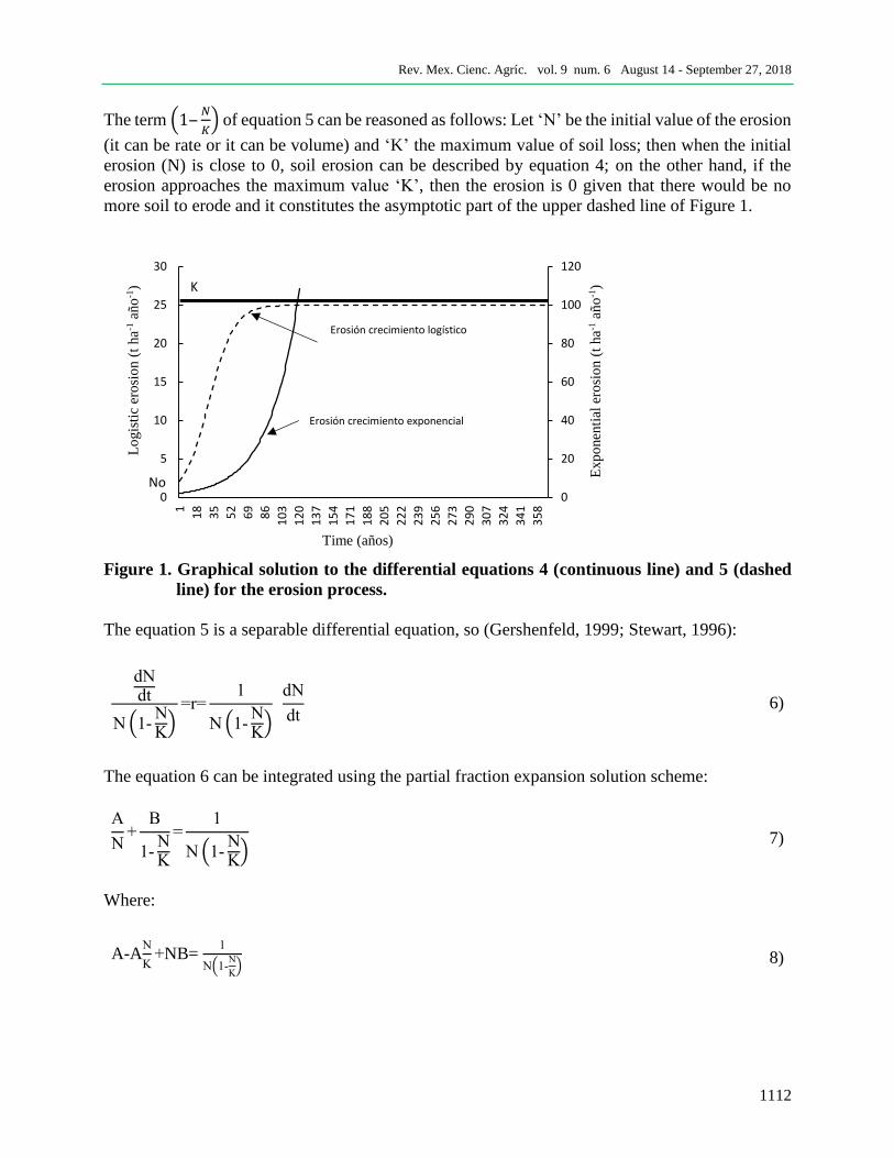
The term (1‒𝑁
𝐾) of equation 5 can be reasoned as follows: Let ‘N’ be the initial value of the erosion
(it can be rate or it can be volume) and ‘K’ the maximum value of soil loss; then when the initial
erosion (N) is close to 0, soil erosion can be described by equation 4; on the other hand, if the
erosion approaches the maximum value ‘K’, then the erosion is 0 given that there would be no
more soil to erode and it constitutes the asymptotic part of the upper dashed line of Figure 1.
Figure 1. Graphical solution to the differential equations 4 (continuous line) and 5 (dashed
line) for the erosion process.
The equation 5 is a separable differential equation, so (Gershenfeld, 1999; Stewart, 1996):
dNdt
N (1-NK
)=r=
1
N (1-NK
) dN
dt 6)
The equation 6 can be integrated using the partial fraction expansion solution scheme:
A
N+
B
1-NK
=1
N (1-NK
) 7)
Where:
A-AN
K+NB=
1
N(1-N
K) 8)
0
20
40
60
80
100
120
0
5
10
15
20
25
30
1
18
35
52
69
86
10
3
12
0
13
7
15
4
17
1
18
8
20
5
22
2
23
9
25
6
27
3
29
0
30
7
32
4
34
1
35
8
Ero
sio
n e
xpo
nen
cial
To
n.h
a-1 .a
ño
-1)
(año
-1)
Ero
sió
n lo
gíst
ica
(To
n.h
a-1 a
ño
-1 )
Tiempo (años)
Erosión crecimiento exponencial
Erosión crecimiento logístico
No
K
Lo
gis
tic
ero
sio
n (
t ha-1
año
-1)
Exp
onen
tial
ero
sio
n (
t ha-1
añ
o-1
)
Time (años)
Rev. Mex. Cienc. Agríc. vol. 9 num. 6 August 14 - September 27, 2018
1113
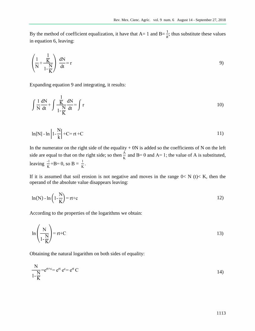
By the method of coefficient equalization, it have that A= 1 and B= 1
𝐾; thus substitute these values
in equation 6, leaving:
(1
N+
1K
1-NK
) dN
dt= r 9)
Expanding equation 9 and integrating, it results:
∫1
N
dN
dt+ ∫
1K
1-NK
dN
dt= ∫ r 10)
ln|N| - ln |1-N
k| +C= rt +C 11)
In the numerator on the right side of the equality + 0N is added so the coefficients of N on the left
side are equal to that on the right side; so then A
K and B= 0 and A= 1; the value of A is substituted,
leaving -1
K+B= 0, so B =
1
K.
If it is assumed that soil erosion is not negative and moves in the range 0< N (t)< K, then the
operand of the absolute value disappears leaving:
ln(N) - ln (1-N
K) = rt+c 12)
According to the properties of the logarithms we obtain:
ln (N
1-NK
) = rt+C 13)
Obtaining the natural logarithm on both sides of equality:
N
1-NK
=ert+c= ert ec= ert C 14)
Rev. Mex. Cienc. Agríc. vol. 9 num. 6 August 14 - September 27, 2018
1114
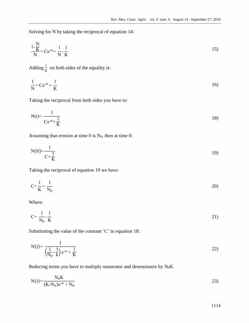
Solving for N by taking the reciprocal of equation 14:
1-NK
N= Ce-rt=
1
N-
1
K
15)
Adding 1
K on both sides of the equality is:
1
N= Ce-rt +
1
K 16)
Taking the reciprocal from both sides you have to:
N(t)= 1
Ce-rt+1K
18)
Assuming that erosion at time 0 is N0, then at time 0:
N(0)=1
C+1K
19)
Taking the reciprocal of equation 19 we have:
C+1
K=
1
N0
20)
Where:
C= 1
N0
-1
K 21)
Substituting the value of the constant ‘C’ in equation 18:
N(t)= 1
(1
N0-1k
) e-rt + 1K
22)
Reducing terms you have to multiply numerator and denominator by N0K.
N(t)=N0K
(K-N0)e-rt + N0
23)
Rev. Mex. Cienc. Agríc. vol. 9 num. 6 August 14 - September 27, 2018
1115
Equation 23 is the solution to the differential equation 5. er(0)= 1.
Parameterization of the logistic model
The logistic model of erosion (equation 23) considers three parameters in its structure: the rate of
erosion ‘r’, the initial state of erosion (No) and the maximum erosion or maximum erosion limit
(K) (Figure 1).
The model operates on any time scale ‘t’, for the case of erosion and in order to obtain an
objective assessment of what the loss of soil in some locality might be, the annual scale is
recommended. So, to obtain the parameter ‘r’; it is necessary to have data of erosion field
observed over time. For the experimental basin of the INIFAP in the municipality of San Luis
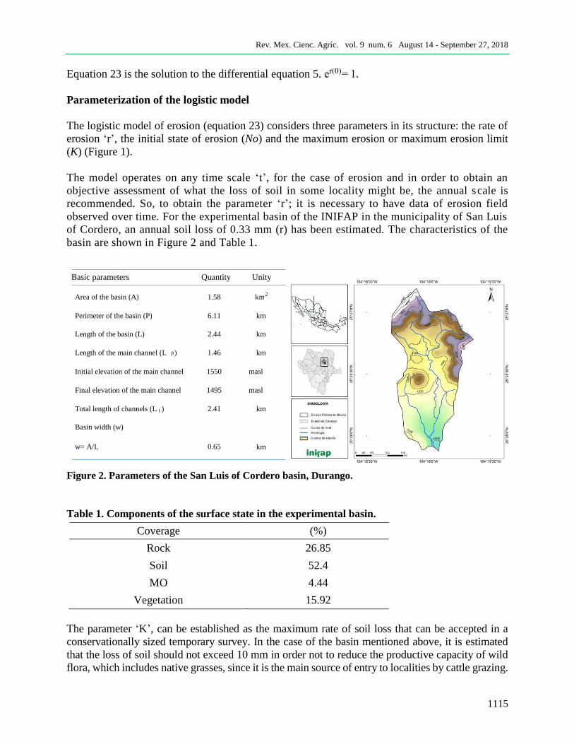
of Cordero, an annual soil loss of 0.33 mm (r) has been estimated. The characteristics of the
basin are shown in Figure 2 and Table 1.
Figure 2. Parameters of the San Luis of Cordero basin, Durango.
Table 1. Components of the surface state in the experimental basin.
Coverage (%)
Rock 26.85
Soil 52.4
MO 4.44
Vegetation 15.92
The parameter ‘K’, can be established as the maximum rate of soil loss that can be accepted in a
conservationally sized temporary survey. In the case of the basin mentioned above, it is estimated
that the loss of soil should not exceed 10 mm in order not to reduce the productive capacity of wild
flora, which includes native grasses, since it is the main source of entry to localities by cattle grazing.
Basic parameters Quantity Unity
Area of the basin (A) 1.58 km 2
Perimeter of the basin (P) 6.11 km
Length of the basin (L) 2.44 km
Length of the main channel (L p ) 1.46 km
Initial elevation of the main channel 1550 masl
Final elevation of the main channel 1495 masl
Total length of channels (L t ) 2.41 km
Basin width (w)
0.65 km w= A/L
Rev. Mex. Cienc. Agríc. vol. 9 num. 6 August 14 - September 27, 2018
1116
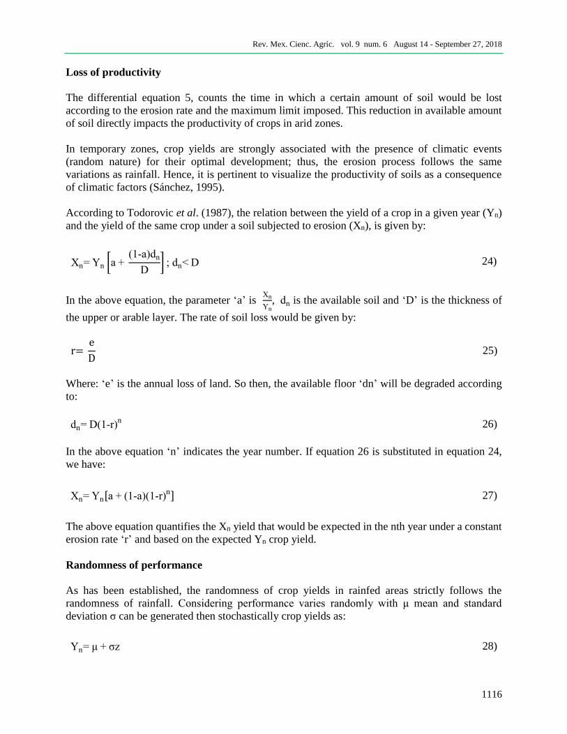
Loss of productivity
The differential equation 5, counts the time in which a certain amount of soil would be lost
according to the erosion rate and the maximum limit imposed. This reduction in available amount
of soil directly impacts the productivity of crops in arid zones.
In temporary zones, crop yields are strongly associated with the presence of climatic events
(random nature) for their optimal development; thus, the erosion process follows the same
variations as rainfall. Hence, it is pertinent to visualize the productivity of soils as a consequence
of climatic factors (Sánchez, 1995).
According to Todorovic et al. (1987), the relation between the yield of a crop in a given year (Yn)
and the yield of the same crop under a soil subjected to erosion (Xn), is given by:
Xn= Yn [a + (1-a)dn
D] ; dn< D 24)
In the above equation, the parameter ‘a’ is Xn
Yn, dn is the available soil and ‘D’ is the thickness of
the upper or arable layer. The rate of soil loss would be given by:
r= e
D 25)
Where: ‘e’ is the annual loss of land. So then, the available floor ‘dn’ will be degraded according
to:
dn= D(1-r)n 26)
In the above equation ‘n’ indicates the year number. If equation 26 is substituted in equation 24,
we have:
Xn= Yn[a + (1-a)(1-r)n] 27)
The above equation quantifies the Xn yield that would be expected in the nth year under a constant
erosion rate ‘r’ and based on the expected Yn crop yield.
Randomness of performance
As has been established, the randomness of crop yields in rainfed areas strictly follows the
randomness of rainfall. Considering performance varies randomly with μ mean and standard
deviation σ can be generated then stochastically crop yields as:
Yn= μ + σz 28)
Rev. Mex. Cienc. Agríc. vol. 9 num. 6 August 14 - September 27, 2018
1117
Being z:
z= [-2ln(rnd1)]0.5cos[2π(rnd2)] 29)
Where: rnd1, 2 are random numbers with μ= 0 and σ= 1.
Parameterization of the productivity model
The parameter ‘a’ of equation 27 is the quotient between crop yield under non-erosion conditions
(naturally preserved soil, Xn) and crop yield under eroded soil. These values can be obtained from
empirical experience or resort to literature in the context. Thus, Table 2 shows guide values to
obtain this value.
Table 2. Reduction of the yield in the corn crop due to the loss of soil (Mokma and Siez, 1992).
Degree of erosion Average performance (t ha-1)
Light 7.34
Moderate 7.09
Severe 5.83
Other authors such as Mbagwu (1988) obtained functional relationships between maize crop yield
and soil erosion in plots with induced erosion. For the first year of study he found:
Ya = 33.2761e−0.1621x with R2= 0.998 and for the second: Yb = 11.6116e−0.1489x with R2= 0.985.
In these regressions ‘x’ is the soil erosion expressed in cm and Ya, Yb are the annual yields
(t ha-1).
For the quantification of the parameter ‘r’, it is necessary to establish the thickness of the soil
layer that is interesting to conserve (D), usually this can be defined by the arable layer (in
seasonal and irrigation agriculture) or that layer capable of being eroded more easily in
pastures. On the other hand, the parameter ‘e’ of equation 25 is the current erosion rate: for
example, as already noted, in the experimental basin of INIFAP in the municipality of San Luis
of Cordero, Durango, the observed rate of erosion during 2016, in three events is 0.44 mm year -
1 on average. The previous thing after analyzing the sedigrams (variation of the solids in
suspension in the time measured in the runoff), product of rainy events (Figure 3).
However, given the lack of this value, the model can be manipulated with different erosion
rates and soil depths to verify what would be the loss in productivity of the crop in different
management scenarios.
Rev. Mex. Cienc. Agríc. vol. 9 num. 6 August 14 - September 27, 2018
1118
Figure 3. Sampling to determine the concentration of suspended solids in a runoff event during
August 2016. INIFAP experimental basin, San Luis of Cordero, Durango.
Results and discussion
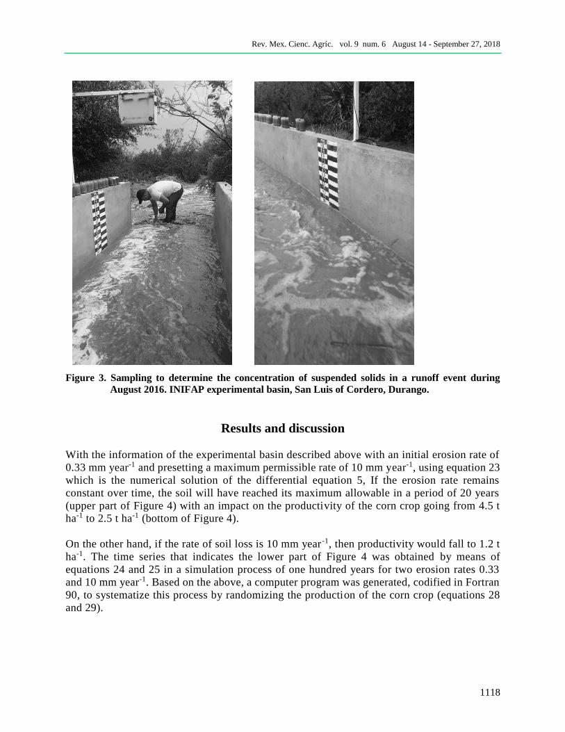
With the information of the experimental basin described above with an initial erosion rate of
0.33 mm year-1 and presetting a maximum permissible rate of 10 mm year-1, using equation 23
which is the numerical solution of the differential equation 5, If the erosion rate remains
constant over time, the soil will have reached its maximum allowable in a period of 20 years
(upper part of Figure 4) with an impact on the productivity of the corn crop going from 4.5 t
ha-1 to 2.5 t ha-1 (bottom of Figure 4).
On the other hand, if the rate of soil loss is 10 mm year -1, then productivity would fall to 1.2 t
ha-1. The time series that indicates the lower part of Figure 4 was obtained by means of
equations 24 and 25 in a simulation process of one hundred years for two erosion rates 0.33
and 10 mm year-1. Based on the above, a computer program was generated, codified in Fortran
90, to systematize this process by randomizing the production of the corn crop (equations 28
and 29).
Rev. Mex. Cienc. Agríc. vol. 9 num. 6 August 14 - September 27, 2018
1119
- 1 )
Figure 4. Model assembly. Logistic model for the prediction of abatement of soil depth by erosion (A)
and time series of loss of soil productivity and its impact on maize crop yield (B).
The loss of productivity is a reflection of the loss of soil depth with the consequent reduction in
moisture retention and fertility.
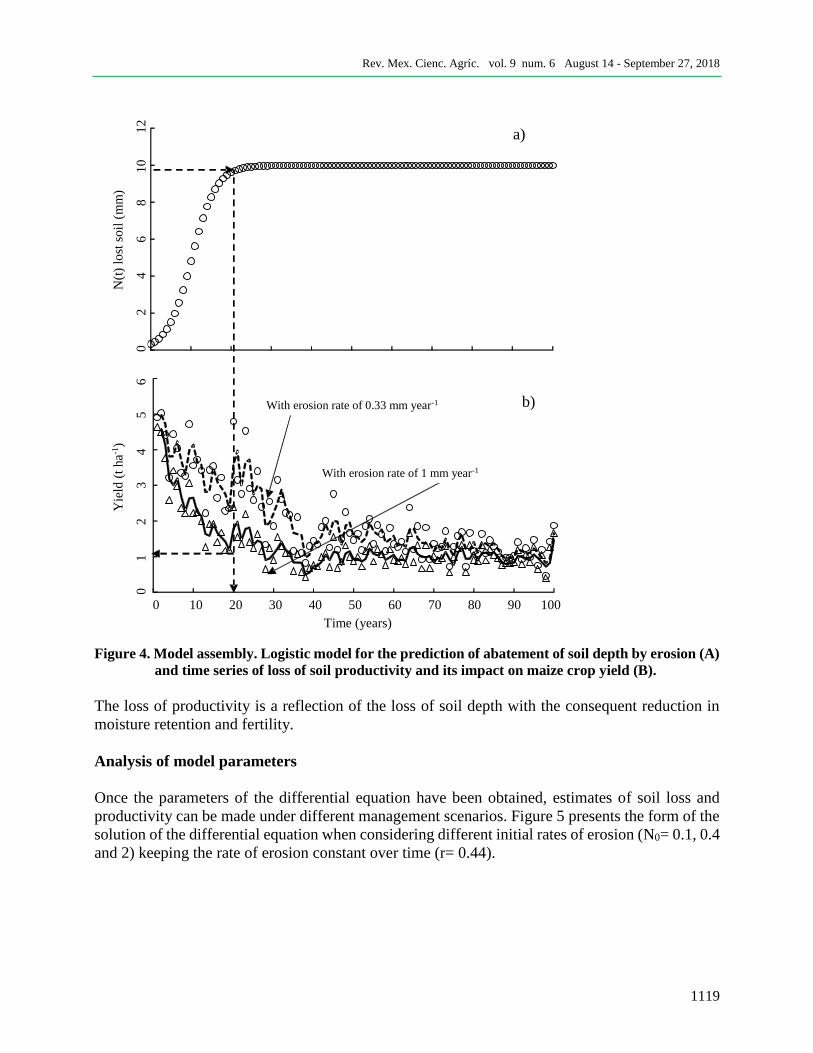
Analysis of model parameters
Once the parameters of the differential equation have been obtained, estimates of soil loss and
productivity can be made under different management scenarios. Figure 5 presents the form of the
solution of the differential equation when considering different initial rates of erosion (N0= 0.1, 0.4
and 2) keeping the rate of erosion constant over time (r= 0.44).
b) With erosion rate of 0.33 mm year-1
Yie
ld (
t ha-1
)
N(t
) lo
st s
oil
(m
m)
0
1
2
3
4
5
6
0
2
4
6
8
10
12
With erosion rate of 1 mm year-1
0 10 20 30 40 50 60 70 80 90 100
Time (years)
a)
Rev. Mex. Cienc. Agríc. vol. 9 num. 6 August 14 - September 27, 2018
1120
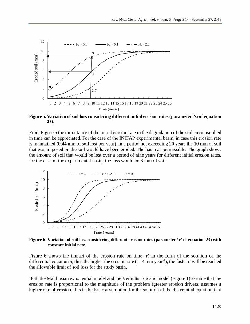
Figure 5. Variation of soil loss considering different initial erosion rates (parameter N0 of equation
23).
From Figure 5 the importance of the initial erosion rate in the degradation of the soil circumscribed
in time can be appreciated. For the case of the INIFAP experimental basin, in case this erosion rate
is maintained (0.44 mm of soil lost per year), in a period not exceeding 20 years the 10 mm of soil
that was imposed on the soil would have been eroded. The basin as permissible. The graph shows
the amount of soil that would be lost over a period of nine years for different initial erosion rates,
for the case of the experimental basin, the loss would be 6 mm of soil.
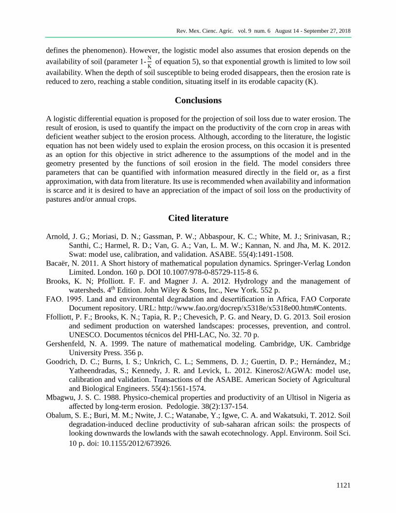
Figure 6. Variation of soil loss considering different erosion rates (parameter ‘r’ of equation 23) with
constant initial rate.
Figure 6 shows the impact of the erosion rate on time (r) in the form of the solution of the
differential equation 5, thus the higher the erosion rate (r= 4 mm year-1), the faster it will be reached
the allowable limit of soil loss for the study basin.
Both the Malthusian exponential model and the Verhults Logistic model (Figure 1) assume that the
erosion rate is proportional to the magnitude of the problem (greater erosion drivers, assumes a
higher rate of erosion, this is the basic assumption for the solution of the differential equation that
0
2
4
6
8
10
12
1 2 3 4 5 6 7 8 9 10 11 12 13 14 15 16 17 18 19 20 21 22 23 24 25 26
Ero
ded
so
il (
mm
)
Time (yeras)
N0 = 0.1 N0 = 0.4 N0 = 2.0
9
6
2.7
0
2
4
6
8
10
12
1 3 5 7 9 11 13 15 17 19 21 23 25 27 29 31 33 35 37 39 41 43 45 47 49 51
Ero
ded
so
il (
mm
)
Time (years)
r = 4 r = 0.2 r = 0.3
Rev. Mex. Cienc. Agríc. vol. 9 num. 6 August 14 - September 27, 2018
1121
defines the phenomenon). However, the logistic model also assumes that erosion depends on the
availability of soil (parameter 1-N
K of equation 5), so that exponential growth is limited to low soil
availability. When the depth of soil susceptible to being eroded disappears, then the erosion rate is
reduced to zero, reaching a stable condition, situating itself in its erodable capacity (K).
Conclusions
A logistic differential equation is proposed for the projection of soil loss due to water erosion. The
result of erosion, is used to quantify the impact on the productivity of the corn crop in areas with
deficient weather subject to the erosion process. Although, according to the literature, the logistic
equation has not been widely used to explain the erosion process, on this occasion it is presented
as an option for this objective in strict adherence to the assumptions of the model and in the
geometry presented by the functions of soil erosion in the field. The model considers three
parameters that can be quantified with information measured directly in the field or, as a first
approximation, with data from literature. Its use is recommended when availability and information
is scarce and it is desired to have an appreciation of the impact of soil loss on the productivity of
pastures and/or annual crops.
Cited literature
Arnold, J. G.; Moriasi, D. N.; Gassman, P. W.; Abbaspour, K. C.; White, M. J.; Srinivasan, R.;
Santhi, C.; Harmel, R. D.; Van, G. A.; Van, L. M. W.; Kannan, N. and Jha, M. K. 2012.
Swat: model use, calibration, and validation. ASABE. 55(4):1491-1508.
Bacaër, N. 2011. A Short history of mathematical population dynamics. Springer-Verlag London
Limited. London. 160 p. DOI 10.1007/978-0-85729-115-8 6.
Brooks, K. N; Pfolliott. F. F. and Magner J. A. 2012. Hydrology and the management of
watersheds. 4th Edition. John Wiley & Sons, Inc., New York. 552 p.
FAO. 1995. Land and environmental degradation and desertification in Africa, FAO Corporate
Document repository. URL: http://www.fao.org/docrep/x5318e/x5318e00.htm#Contents. Ffolliott, P. F.; Brooks, K. N.; Tapia, R. P.; Chevesich, P. G. and Neary, D. G. 2013. Soil erosion
and sediment production on watershed landscapes: processes, prevention, and control.
UNESCO. Documentos técnicos del PHI-LAC, No. 32. 70 p.
Gershenfeld, N. A. 1999. The nature of mathematical modeling. Cambridge, UK. Cambridge
University Press. 356 p.
Goodrich, D. C.; Burns, I. S.; Unkrich, C. L.; Semmens, D. J.; Guertin, D. P.; Hernández, M.;
Yatheendradas, S.; Kennedy, J. R. and Levick, L. 2012. Kineros2/AGWA: model use,
calibration and validation. Transactions of the ASABE. American Society of Agricultural
and Biological Engineers. 55(4):1561-1574.
Mbagwu, J. S. C. 1988. Physico-chemical properties and productivity of an Ultisol in Nigeria as
affected by long-term erosion. Pedologie. 38(2):137-154.
Obalum, S. E.; Buri, M. M.; Nwite, J. C.; Watanabe, Y.; Igwe, C. A. and Wakatsuki, T. 2012. Soil
degradation-induced decline productivity of sub-saharan african soils: the prospects of
looking downwards the lowlands with the sawah ecotechnology. Appl. Environm. Soil Sci.
10 p. doi: 10.1155/2012/673926.
Rev. Mex. Cienc. Agríc. vol. 9 num. 6 August 14 - September 27, 2018
1122
Pearl, R. and Reed, L. J. 1920. On the rate of growth of the population of the United States since
1790 and its mathematical representation. Proc. Natl. Acad. Sci. 6:275-288.
http://www.pnas.org/search?fulltext=pearl+and+reed&submit=yes&x=0&y=0.
Sánchez, C. I. 1995. Erosión y productividad en la Comarca Lagunera. Folleto científico núm. 4.
INIFAP ORSTOM. 25 p.
Sánchez, C. I. 2005. Fundamentos para el aprovechamiento integral del agua. Una aproximación
de simulación de procesos. Libro científico núm. 2. INIFAP CENID RASPA. 272 p.
Skoldberg, E. 2012. The logistic model for population growth. School of Mathematics etc. National
University of Ireland, Galway. Ireland.
Stewart, J. 1996. Calculus: concepts and context. Brooks cole. Book 4th edition. 493 -508 pp.
Thornes, B. J. 2004. Stability and insestability in the management of Mediterranean desertification.
In: Wainwright, J. and Mulligan, M. (Eds.). Environmental Modelling. Finding Simplicity
in Complexity. John Wiley & Sons, Ltd. 303-315 p.
Van der Knijff J. M.; Jones R. J. A. and Montanarella, L. 2000. Soil erosion assessment risk in
Europe. European Commission Directorate General Jrc Joint Research Centre Space
Applications Institute European Soil Bureau. 31 p.
Wainwright, J. and Mulligan, M. 2004. Environmental modelling. Finding simplicity in
complexity. John Wiley & Sons, Ltd. London. 822 p.
Wolfram, S. 2002. A new kind of science. Champaign, IL. Wolfram Media. 918 p.