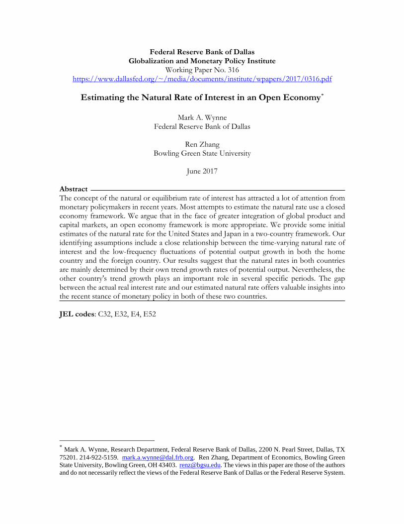
Federal Reserve Bank of Dallas Globalization and Monetary Policy Institute

Working Paper No. 316 https://www.dallasfed.org/~/media/documents/institute/wpapers/2017/0316.pdf

Estimating the Natural Rate of Interest in an Open Economy*

Mark A. Wynne

Federal Reserve Bank of Dallas

Ren Zhang Bowling Green State University

June 2017

Abstract The concept of the natural or equilibrium rate of interest has attracted a lot of attention from monetary policymakers in recent years. Most attempts to estimate the natural rate use a closed economy framework. We argue that in the face of greater integration of global product and capital markets, an open economy framework is more appropriate. We provide some initial estimates of the natural rate for the United States and Japan in a two-country framework. Our identifying assumptions include a close relationship between the time-varying natural rate of interest and the low-frequency fluctuations of potential output growth in both the home country and the foreign country. Our results suggest that the natural rates in both countries are mainly determined by their own trend growth rates of potential output. Nevertheless, the other country's trend growth plays an important role in several specific periods. The gap between the actual real interest rate and our estimated natural rate offers valuable insights into the recent stance of monetary policy in both of these two countries. JEL codes: C32, E32, E4, E52

* Mark A. Wynne, Research Department, Federal Reserve Bank of Dallas, 2200 N. Pearl Street, Dallas, TX 75201. 214-922-5159. mark.a.wynne@dal.frb.org. Ren Zhang, Department of Economics, Bowling Green State University, Bowling Green, OH 43403. renz@bgsu.edu. The views in this paper are those of the authors and do not necessarily reflect the views of the Federal Reserve Bank of Dallas or the Federal Reserve System.

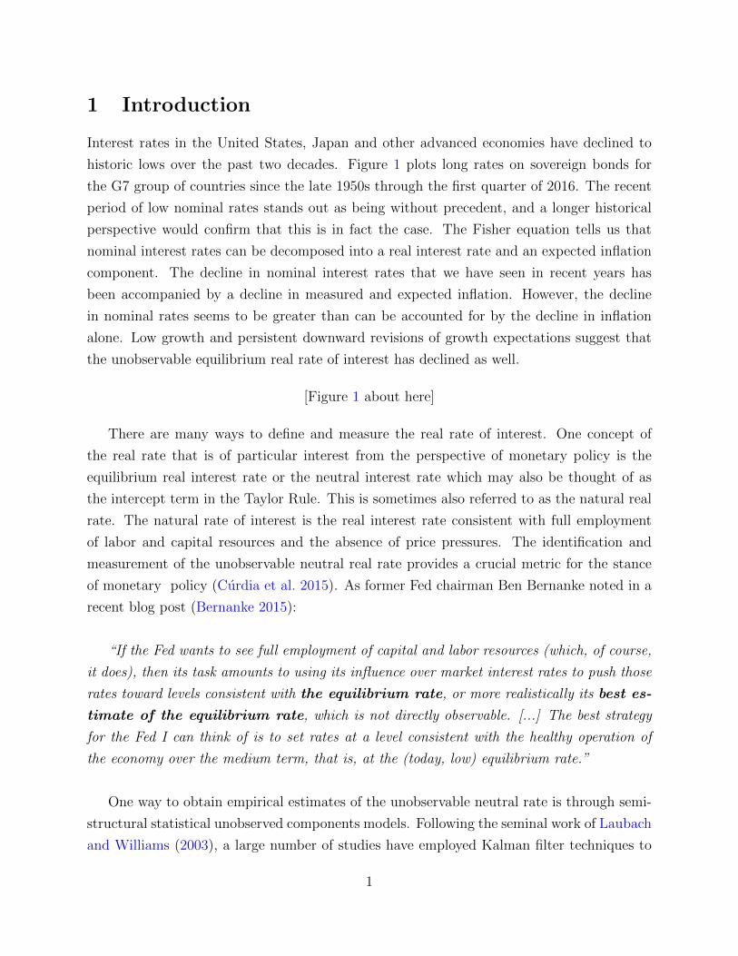
1 Introduction

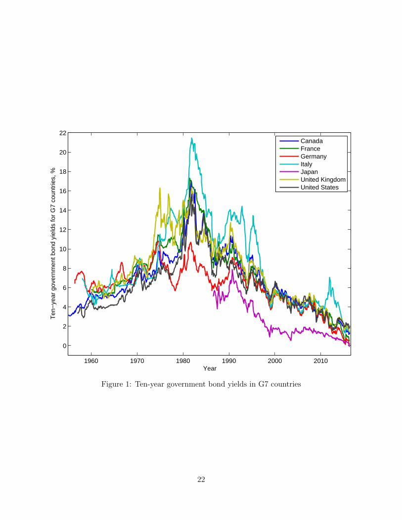
Interest rates in the United States, Japan and other advanced economies have declined to

historic lows over the past two decades. Figure 1 plots long rates on sovereign bonds for

the G7 group of countries since the late 1950s through the first quarter of 2016. The recent

period of low nominal rates stands out as being without precedent, and a longer historical

perspective would confirm that this is in fact the case. The Fisher equation tells us that

nominal interest rates can be decomposed into a real interest rate and an expected inflation

component. The decline in nominal interest rates that we have seen in recent years has

been accompanied by a decline in measured and expected inflation. However, the decline

in nominal rates seems to be greater than can be accounted for by the decline in inflation

alone. Low growth and persistent downward revisions of growth expectations suggest that

the unobservable equilibrium real rate of interest has declined as well.

[Figure 1 about here]

There are many ways to define and measure the real rate of interest. One concept of

the real rate that is of particular interest from the perspective of monetary policy is the

equilibrium real interest rate or the neutral interest rate which may also be thought of as

the intercept term in the Taylor Rule. This is sometimes also referred to as the natural real

rate. The natural rate of interest is the real interest rate consistent with full employment

of labor and capital resources and the absence of price pressures. The identification and

measurement of the unobservable neutral real rate provides a crucial metric for the stance

of monetary policy (Curdia et al. 2015). As former Fed chairman Ben Bernanke noted in a

recent blog post (Bernanke 2015):

“If the Fed wants to see full employment of capital and labor resources (which, of course,

it does), then its task amounts to using its influence over market interest rates to push those

rates toward levels consistent with the equilibrium rate, or more realistically its best es-

timate of the equilibrium rate, which is not directly observable. [...] The best strategy

for the Fed I can think of is to set rates at a level consistent with the healthy operation of

the economy over the medium term, that is, at the (today, low) equilibrium rate.”

One way to obtain empirical estimates of the unobservable neutral rate is through semi-

structural statistical unobserved components models. Following the seminal work of Laubach

and Williams (2003), a large number of studies have employed Kalman filter techniques to

1

jointly estimate several unobservable variables – the neutral real interest rate, the level of

potential output and the trend rate of growth of output – linking the neutral real interest rate

closely to the trend growth rate (e.g., see Laubach and Williams 2003, Clark and Kozicki

2005, Mesonnier and Renne 2007, Trehan and Wu 2007, Barsky et al. 2014, Berger and

Kempa 2014, Umino 2014, Pescatori and Turunen 2015, Wynne and Zhang 2016, Holston

et al. 2017). Nevertheless, almost all of the previous work on this topic has focused on a

closed economy or small open economy setting. In light of the increasing integration of global

product and capital markets, it is worth examining the extent to which foreign or external

factors might impact estimates of the domestic natural rate. In what follows, we extend

the Laubach and Williams (2003) model to a two-country setting. Motivated by Clarida

et al. (2002), we link the domestic natural rate to the trend rate of growth in both the home

country and the foreign country. Then we implement this framework by taking the United

States as the home country and Japan as the foreign country. By estimating the model using

data from 1961Q1 to 2014Q3 with Bayesian methods, we obtain three main results.

First, trend potential output growth rates in both countries have been declining over

time but with distinct patterns. In particular, the U.S. trend growth rate was stable at

around 3 percent prior 2000 but then declined significantly in the first decade of the new

century, bottoming out at 0.5 percent in 2009. On the other hand, Japan’s trend growth

rate plummets in a step-shaped pattern which has experienced three conspicuous falls in the

past half century. Specifically, it decreased from 10 percent in 1968 to 3.9 percent in 1975,

from 5 percent in 1988 to 1.2 percent in 1993 and from 1.5 percent in 2005 to -0.7 percent

in 2008. These distinct differences in the trend growth patterns between the two countries

help identify each of their contributions to the natural rate.

Second, the natural interest rates in both the U.S. and Japan are not only determined

by their own trend growth rate but also the other country’s trend growth rate. Based on our

estimates, the major driver of the natural rate in each country is the country’s own trend

growth rate. Nevertheless, the other country’s trend growth indeed contributes to a greater

or lesser extent at different times. For instance, Japan’s trend growth drives down the U.S.

natural rate fundamentally during the three periods when Japan’s trend growth is in sharp

decline. Moreover, the more recent recovery in the U.S. economy after 2009 also helps raise

Japan’s natural rate even when its own economy is still in stagnation.

Lastly, the estimated gap between the actual real interest rate and the natural rate

provides insights into the stance of monetary policy in U.S. and Japan in recent years. For

instance, the U.S. natural rate decreased from 1.4 percent to 1.2 percent between 2004Q2

to 2006Q3 while the nominal federal funds rate rose from 1 percent to 5.3 percent during

2

the same period. After 2006Q3, the U.S. natural rate declined further, until it reached a

historically low level of -1.0 percent in 2009Q1, and then remained negative until 2012Q4.

The negative natural rate can be seen as justifying the Fed’s unconventional monetary policy

actions during this period in the form of Large Scale Asset Purchases (LSAPs) and forward

guidance which lowered the real interest rate when the nominal interest rate reached the

zero lower bound. On the other side, Japan’s natural rate declines in a step-shaped pattern

along with its trend potential output growth rate. In 1991Q3, the Bank of Japan raised the

nominal short-term interest rate to around 8 percent in spite of the sharply declining natural

rate. The real interest rate gap reached an almost historically high level 4.7 percent at that

time. This sharp tightening of policy contributed to the bursting of the asset price bubble

and ushered in the era of the “lost decades”. In February 1999, the Bank of Japan lowered

its policy rate effectively to zero to combat negative inflation.1 However, our estimation

demonstrates that this Zero Interest Rate Policy was not so expansionary since the natural

rate also remained at a low level close to zero at that time. The natural rate stays negative

since 2000Q2 which makes Japan’s Zero Interest Rate Policy quite contractionary until the

Abe government’s aggressive Quantitative and Qualitative Easing Program in 2013 started

to take effect by gradually raising inflation expectations. The ensuing negative natural rate

supported the Abe government’s more aggressive Quantitative Easing program announced

in October 2014 and the negative interest rate policy adopted in 2016.

The rest of the paper is organized as follows. In the next section, we lay out the basic

structure of our two-country model. Section 3 describes the data. Section 4 presents the

main estimation results. Section 5 discusses the robustness analysis, and section 6 concludes.

2 Model Description

2.1 Motivation

Our point of departure is the idea that as a result of greater integration of global goods and

capital markets, foreign as well as domestic factors are likely to be important in determining

the level of the natural rate of interest. The key motivating equation in the Laubach and

Williams (2003) paper is the following version of the relationship between the real rate of in-

terest, r, and the rate of growth of consumption, gc, that falls out of almost any intertemporal

household optimization problem:

1This Zero Interest Rate Policy (ZIRP) was implemented from 1999M2-2000M8, 2001M3-2006M7 and2009M1 to present.

3

r = σgc + θ, (1)

where σ is the inverse of intertemporal elasticity of substitution and θ is the pure rate

of time preference. Laubach and Williams use this theoretical relationship to motivate a

relationship between the unobserved natural real rate of interest rt and the trend rate of

growth of potential output gt in a closed economy:

rt = cgt + zt, (2)

where zt captures other determinants of the natural rate of interest.An obvious extension

of this equation to an open economy setting would be something like the following:

rt = cgt + c∗tg∗t + zt (3)

where g∗t now denotes the trend rate of growth in the foreign economy. With perfect risk

sharing and fully integrated financial markets, the real interest rate in both the home and

foreign country should equal the world rate, which in turn should be some average of the

trend growth rates in the home and foreign economies. 2 The inclusion of the zt term in the

equation can be thought of as capturing – in addition to other determinants of the natural

rate – any distortions that limit international risk sharing. 3 We will take this as the point

of departure for our extension of the Laubach and Williams (2003) model to a two-country

setting.

2.2 Statistical model

Our benchmark statistical model is a straightforward extension of the closed economy model

of Laubach and Williams (2003). We specify two IS equations for the home country (with

superscript h) and the foreign country (with superscript f) with the output gap (y = y− y)

being determined by its own lags and lags of the real policy rate gap:

2For an early exposition of the determination of the world interest rate in an endowment economy seeFrenkel and Razin (1986).

3Clarida et al. (2002) show that in a standard New Keynesian open economy setting with no capital, theneutral equilibrium real interest rate consistent with flexible prices in the domestic economy is given by anaverage of the (expected) growth rates of domestic potential (flex-price) output, yht , and the growth rate of

actual (sticky price) foreign output, yft :rht = σ0Et{∆yht+1} + κ0Et{∆yft+1}, where σ0 = σ − γ(σ − 1) andκ0 = γ(σ − 1) so that σ0 + κ0 equals the inverse of intertemporal elasticity of substitution σ, and γ is theshare of home spending on the foreign good.

4

yht = ahy,1yht−1 + ahy,2y

ht−2 +

ahr2

2∑j=1

(rht−j − rht−j) + εhy,t, (4)

and

yft = afy,1yft−1 + afy,2y

ft−2 +

afr2

2∑j=1

(rft−j − rft−j) + εfy,t. (5)

We add two Phillips curves for the home country and the foreign country where the

(core) inflation rate πt is determined by its own lags, the lagged output gap yt−1, two other

variables measuring relative price shocks — core import price inflation πIt and lagged crude

imported petroleum price πOt — and a serially uncorrelated disturbance επt:

πht = bhπ(L)πht + bhy yht−1 + bhπI (π

I,ht − πht ) + bhπO(πO,ht−1 − πht−1) + εhπ,t, (6)

and

πft = bfπ(L)πft + bfy yft−1 + bf

πI(πI,ft − π

ft ) + bf

πO(πO,ft−1 − π

ft−1) + εfπ,t. (7)

We include eight lags of inflation in the equations above. For parsimony, we impose

the restriction — not rejected by our sample — that the sum of the coefficients on lagged

inflation must equal unity.4 We also assume that the coefficients on the second through

fourth lags to be equal to each other as are the coefficients on the fifth to eighth lags, i.e.,

bπ(L)πt−1 = bπ,1πt−1 + bπ,23

∑4i=2 πt−i + (1−bπ,1−bπ,2)

4

∑8i=5 πt−i.

Equations (4) to (7) are the measurement equations of our benchmark model. Immedi-

ately following the motivation equation (3), we assume a law of motion for the natural rate

of interest r in each country as follows:

rht = chhght + chfg

ft + zht , (8)

and

rft = cfhght + cffg

ft + zft , (9)

where ght is our estimate of home country trend growth of potential output and gft cor-

responds to the foreign country trend growth.

4This is a standard restriction to ensure that the Phillips curve obeys the Natural Rate Hypothesis inthe long run.

5

Finally, the transition equation for potential output in each country is assumed to be

given by5:

yht = yht−1 + 0.25ght−1 + εhy,t, (10)

and

yft = yft−1 + 0.25gft−1 + εfy,t. (11)

And again following Laubach and Williams (2003) we assume that the trend rate of

growth of potential output in each country follows a random walk:

ght = ght−1 + εhg,t, (12)

and

gft = gft−1 + εfg,t. (13)

We assume that all the shocks above are serially uncorrelated and uncorrelated with one

another. As detailed in the Appendix, the model has a state-space representation:

Yt = HSt + AXt + ut, (14)

and

St = FSt−1 + vt, (15)

where:

Yt =(yht , πht , yft , πft

)′, ut =

(εhy,t, εhπ,t, εfy,t, εfπ,t

)′,

Xt =

(yht−1, yht−2, rht−1, rht−2, πht−1, πht−2,4 πht−5,8, πO,ht−1 − πht−1, πI,ht − πht . . .yft−1, yft−2, rft−1, rft−2, πft−1, πft−2,4, πft−5,8, πO,ft−1 − π

ft−1, πI,ft − π

ft

)′,

St =(yht , yht−1, yht−2 ght−1, ght−2, zht−1, zht−2, yft , yft−1, yft−2 gft−1, gft−2 zft−1, zft−2

)′,

5The coefficient before the annualized trend growth rate gt is 0.25 because our output data are quarterly.This is consistent with the setup in other studies such as Trehan and Wu (2007).

6

vt =(εhy,t, 0, 0, εhg,t, 0, εhz,t, 0, εfy,t, 0, 0, εfg,t, 0, εfz,t, 0

)′.

3 Data

The model is estimated using quarterly data from 1961Q1 to 2014Q3. We take the U.S. as

the home country and we use Laubach and Williams (2003) data for that part of the model,

extended through 2014.6 The variable yht is measured as the log of real chain-weighted GDP

in billions of chained 2009 dollars. We use quarterly averages of the daily annualized effective

nominal federal funds rate as our measure of the policy rate. For the period prior to 1965,

we use the Federal Reserve Bank of New York’s discount rate. We measure the inflation rate

πht as the core PCE inflation rate which is the annualized quarterly growth rate of the price

index for personal consumption expenditures excluding food and energy. To construct the

ex ante real policy rate rht , we compute the expectation of average inflation over the four

quarters ahead from a univariate AR(3) model of inflation estimated over the 40 quarters

prior to the date at which expectations are being formed.7 Finally, the relative price variables

included in the Phillips curve are the FRB/US price index for imports excluding petroleum

πI,ht and the FRB/US crude oil import price inflation πO,ht .8

We select Japan as the foreign country for several reasons. Firstly, for most of our sam-

ple, Japan was the second largest economy in the world and played an important role in

international financial markets.9 Moreover, Japan has maintained a tight economic and fi-

nancial relationship with U.S. which makes it meaningful to explore how those two countries

interact in determining the natural rate.10 In addition, the pattern of Japanese trend growth

6Laubach and Williams have updated the data to more recent period. We thank Thomas Laubach forsharing their data with us. We used the Laubach and Williams data so as to facilitate comparison of ourresults with theirs.

7To compute these expectations for the early part of our sample, we need to use inflation data prior to1959Q2, the start of the core PCE inflation series. For these dates, we splice headline PCE inflation to corePCE inflation.

8The HAVER codes for the data series we use are: GDP - GDPH@USECON; Core PCE defla-tor - JCXFE@USECON; Effective Federal Funds Rate - FFED@USECON; FRBNY discount rate -FDWB@USECON; PCE deflator - JC@USECON. The two data series we take from the FRB/US databaseclosely track the following HAVER series: Price index for imports excluding petroleum, computers andsemiconductors - PMENP@USECON (quarterly average available since 1989Q1); Crude imported oil priceinflation - PMEPI@USECON(quarterly average available since 1989Q1).

9On a PPP basis Japan ranked second behind the United States until about 2000 when it was overtakenby China.

10Japanese investors currently hold about 20 percent of U.S. treasury securities outstanding. About 12percent of FDI in the U.S. comes from Japan, down from a peak of 23 percent in 1992.

7

rate is fairly distinguishable from its U.S. counterpart which should help identify its contri-

bution to the natural rate of both the home and foreign country.11 An alternative approach

would be to aggregate multiple countries as the foreign country. In reality, the international

interactions between U.S. and other individual countries are heterogeneous for geographic,

cultural and political reasons. This makes any existing aggregation approach less than ideal

for measuring the total influence of the foreign country (Chudik and Straub 2017). Never-

theless, properly incorporating other advanced economies and emerging countries into the

model could be a possible avenue for future research.

Japanese indicators are constructed in a way comparable to what we do for the U.S.

Real output yft is measured as the log of GDP in 2011 Yen. Following Umino (2014), we

proxy the short-term interest rate using the Tokyo overnight call money market rate. There

is no equivalent of the core PCE price index available for Japan. We measure the inflation

rate πft as the core CPI inflation rate which is the annualized quarterly growth rate of the

consumer price index excluding food and energy. Expected inflation is derived in exactly

the same way as for the U.S. case using an AR(3) model fitted to inflation and estimated

using a 40-quarter rolling window. There are no measures of core import prices published for

Japan, so we use the annualized quarterly rate of change of the overall import price instead

as one of the supply shock variables in the Phillips curve for Japan. Lastly, we measure πO,ft

in the inflation equation as the annualized quarterly growth rate of the import price index

for petroleum, coal and natural gas.12

4 Estimation Results

The model is estimated with a Bayesian approach where we use a Metropolis-Hastings

Markov Chain Monte Carlo (MCMC) algorithm to draw 50,000 draws from the posterior

distribution (with a burn-in sample of 50,000 draws). This yields several benefits compared

to maximum likelihood estimation. First, the Bayesian approach allows us to incorporate

extra information from the literature which reduces the uncertainty around the estimation

of the natural rate, the output gap and the trend growth rate. This is particularly useful in

11The average annual growth rate of GDP in Japan was 10.2 percent in the 1960s, 4.5 percent in the 1970sand the 1980s, 1.4 percent in the 1990s and 1.1 percent from 2000 to 2015. By comparison, the averageannual growth rate of GDP in the U.S. was 4.2 percent in the 1960s, 3.3 percent in the 1970s, 3.2 percent inthe 1980s, 3.3 percent in the 1990s and 2.7 percent from 2000 to 2015.

12The HAVER codes for the data series we use for Japan are as follows: GDP - A158GDPC@OECDNAQ;Core CPI - C158CZCN@OECDMEI; Tokyo overnight call rate - C158IM@IFS; Import prices -H158PFMI@G10; Import price for petroleum, coal and natural gas - H158PFMP@G10.

8

our case since the dimension of both the parameter vector and the state vector are greatly

expanded in our two-country model compared to previous closed economy frameworks. Sec-

ond, the maximum likelihood estimate of the standard deviation of the innovation to the

trend growth process σg tends to be biased towards zero owing to the so-called “pile-up

problem” addressed in Stock (1994). Bayesian methods can avoid this problem by properly

tuning the priors. Finally, Bayesian methods deliver samples from posterior distributions,

thus the finite-sample uncertainty around any object of interest can be precisely delineated.

4.1 Prior distribution of the parameters

Figures 2 and 3 plot the prior and posterior distribution of the parameters while Table 1

reports the associated 90 percent confidence intervals. The prior distribution is assumed

to be Gaussian for all parameters except for the variance parameters which are assumed

to be gamma distributed. We set diffuse priors on all of the coefficient parameters. The

prior means for the coefficients of the home country IS equation, Phillips curve equation,

and the natural rate determination equation are picked based on previous closed-economy

studies in the literature, such as Laubach and Williams (2003), Trehan and Wu (2007) among

others. The corresponding foreign country prior means are set based on results in Umino

(2014) and our own prior research treating Japan as a small open economy.13 The priors for

the international interaction coefficient in the natural rate determination, i.e., chf and cff in

equation (8) and (9), are set loosely with the means respectively set as 0 and 0.5 based on

the prior belief that the international interaction is more important for Japan than for the

U.S.

The priors for the variance of the shock to the trend growth, i.e., σ2g,h and σ2

g,f , and the

priors for the variance of the shock to the other natural rate determinants, i.e., σ2z,h and σ2

z,f ,

are tuned to avoid the so-called “pile-up” problem. Specifically, the prior means for these

two shocks are assigned based on previous work while the associated prior variances are set

to a relatively small interval. The priors of all of the other variance parameters are much

more uninformative, which leaves the task of shock identification to the data.

[Figures 2 and 3 and Table 1 about here]

13The small open economy study is implemented with a model introduced in Berger and Kempa (2014).

9

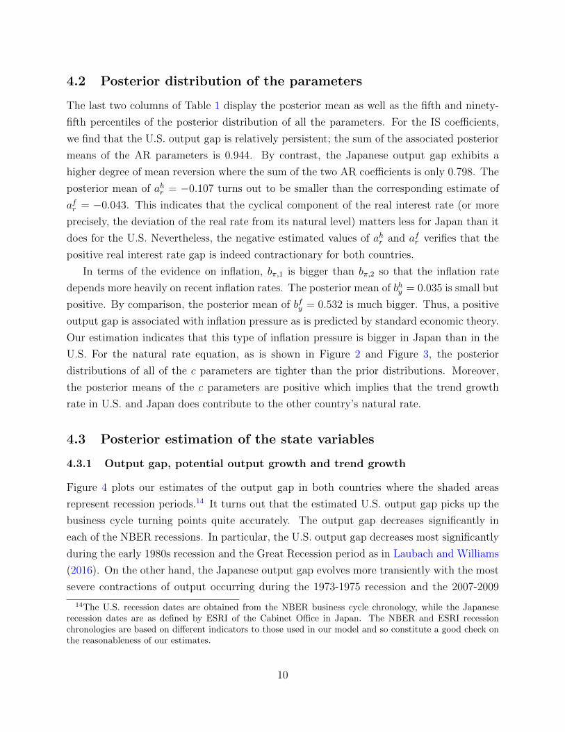
4.2 Posterior distribution of the parameters

The last two columns of Table 1 display the posterior mean as well as the fifth and ninety-

fifth percentiles of the posterior distribution of all the parameters. For the IS coefficients,

we find that the U.S. output gap is relatively persistent; the sum of the associated posterior

means of the AR parameters is 0.944. By contrast, the Japanese output gap exhibits a

higher degree of mean reversion where the sum of the two AR coefficients is only 0.798. The

posterior mean of ahr = −0.107 turns out to be smaller than the corresponding estimate of

afr = −0.043. This indicates that the cyclical component of the real interest rate (or more

precisely, the deviation of the real rate from its natural level) matters less for Japan than it

does for the U.S. Nevertheless, the negative estimated values of ahr and afr verifies that the

positive real interest rate gap is indeed contractionary for both countries.

In terms of the evidence on inflation, bπ,1 is bigger than bπ,2 so that the inflation rate

depends more heavily on recent inflation rates. The posterior mean of bhy = 0.035 is small but

positive. By comparison, the posterior mean of bfy = 0.532 is much bigger. Thus, a positive

output gap is associated with inflation pressure as is predicted by standard economic theory.

Our estimation indicates that this type of inflation pressure is bigger in Japan than in the

U.S. For the natural rate equation, as is shown in Figure 2 and Figure 3, the posterior

distributions of all of the c parameters are tighter than the prior distributions. Moreover,

the posterior means of the c parameters are positive which implies that the trend growth

rate in U.S. and Japan does contribute to the other country’s natural rate.

4.3 Posterior estimation of the state variables

4.3.1 Output gap, potential output growth and trend growth

Figure 4 plots our estimates of the output gap in both countries where the shaded areas

represent recession periods.14 It turns out that the estimated U.S. output gap picks up the

business cycle turning points quite accurately. The output gap decreases significantly in

each of the NBER recessions. In particular, the U.S. output gap decreases most significantly

during the early 1980s recession and the Great Recession period as in Laubach and Williams

(2016). On the other hand, the Japanese output gap evolves more transiently with the most

severe contractions of output occurring during the 1973-1975 recession and the 2007-2009

14The U.S. recession dates are obtained from the NBER business cycle chronology, while the Japaneserecession dates are as defined by ESRI of the Cabinet Office in Japan. The NBER and ESRI recessionchronologies are based on different indicators to those used in our model and so constitute a good check onthe reasonableness of our estimates.

10

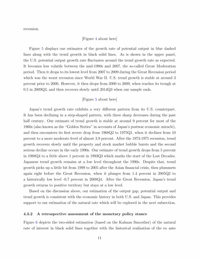
recession.

[Figure 4 about here]

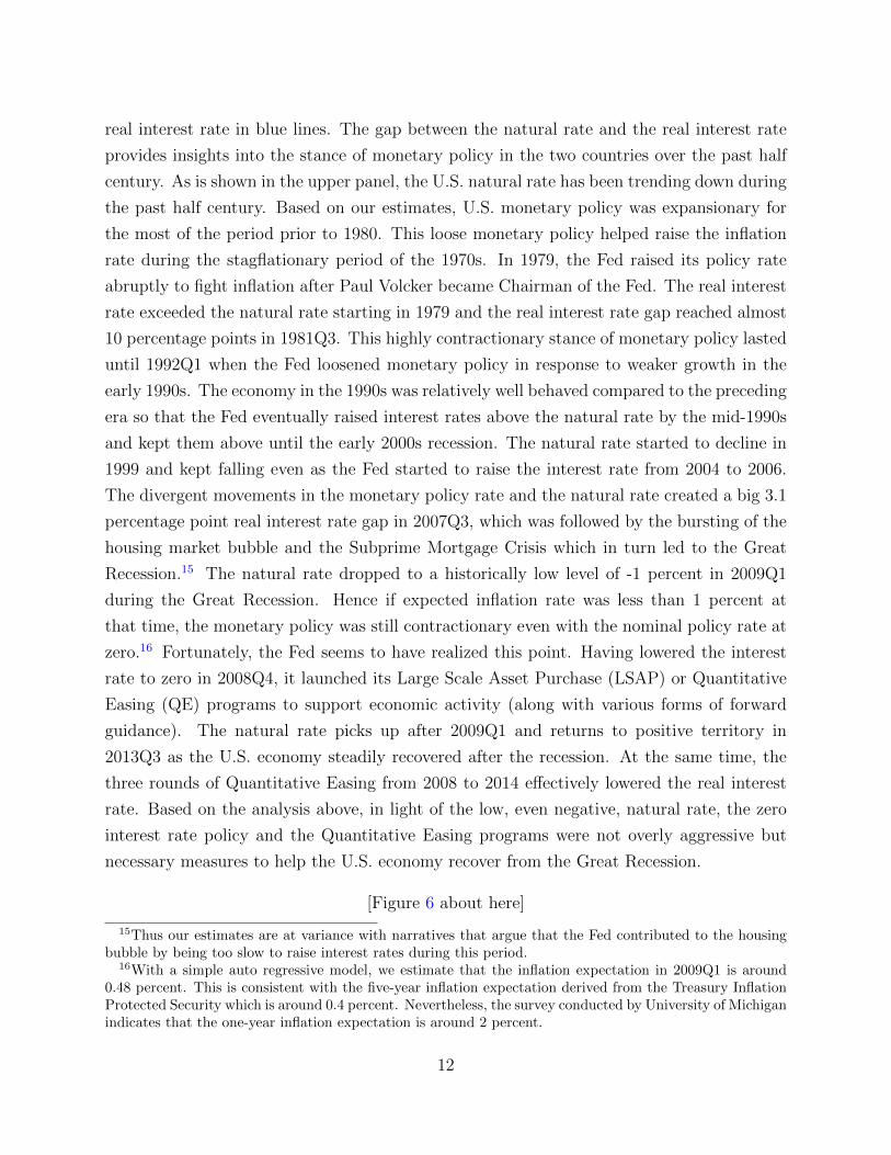
Figure 5 displays our estimates of the growth rate of potential output in blue dashed

lines along with the trend growth in black solid lines. As is shown in the upper panel,

the U.S. potential output growth rate fluctuates around the trend growth rate as expected.

It becomes less volatile between the mid-1980s and 2007, the so-called Great Moderation

period. Then it drops to its lowest level from 2007 to 2009 during the Great Recession period

which was the worst recession since World War II. U.S. trend growth is stable at around 3

percent prior to 2000. However, it then drops from 2000 to 2009, when reaches its trough at

0.5 in 2009Q3, and then recovers slowly until 2014Q3 when our sample ends.

[Figure 5 about here]

Japan’s trend growth rate exhibits a very different pattern from its U.S. counterpart.

It has been declining in a step-shaped pattern, with three sharp decreases during the past

half century. Our estimate of trend growth is stable at around 9 percent for most of the

1960s (also known as the “Golden Sixties” in accounts of Japan’s postwar economic miracle),

and then encounters its first severe drop from 1968Q2 to 1975Q1, when it declines from 10

percent to a more moderate level of almost 3.9 percent. After the 1973-1975 recession, trend

growth recovers slowly until the property and stock market bubble bursts and the second

serious decline occurs in the early 1990s. Our estimate of trend growth drops from 5 percent

in 1988Q4 to a little above 1 percent in 1993Q3 which marks the start of the Lost Decades.

Japanese trend growth remains at a low level throughout the 1990s. Despite that, trend

growth picks up a little bit from 1999 to 2005 after the Asian financial crisis, then plummets

again right before the Great Recession, when it plunges from 1.4 percent in 2005Q2 to

a historically low level -0.7 percent in 2008Q4. After the Great Recession, Japan’s trend

growth returns to positive territory but stays at a low level.

Based on the discussion above, our estimation of the output gap, potential output and

trend growth is consistent with the economic history in both U.S. and Japan. This provides

support to our estimation of the natural rate which will be explored in the next subsection.

4.3.2 A retrospective assessment of the monetary policy stance

Figure 6 depicts the two-sided estimation (based on the Kalman Smoother) of the natural

rate of interest in black solid lines together with the historical realization of the ex ante

11

real interest rate in blue lines. The gap between the natural rate and the real interest rate

provides insights into the stance of monetary policy in the two countries over the past half

century. As is shown in the upper panel, the U.S. natural rate has been trending down during

the past half century. Based on our estimates, U.S. monetary policy was expansionary for

the most of the period prior to 1980. This loose monetary policy helped raise the inflation

rate during the stagflationary period of the 1970s. In 1979, the Fed raised its policy rate

abruptly to fight inflation after Paul Volcker became Chairman of the Fed. The real interest

rate exceeded the natural rate starting in 1979 and the real interest rate gap reached almost

10 percentage points in 1981Q3. This highly contractionary stance of monetary policy lasted

until 1992Q1 when the Fed loosened monetary policy in response to weaker growth in the

early 1990s. The economy in the 1990s was relatively well behaved compared to the preceding

era so that the Fed eventually raised interest rates above the natural rate by the mid-1990s

and kept them above until the early 2000s recession. The natural rate started to decline in

1999 and kept falling even as the Fed started to raise the interest rate from 2004 to 2006.

The divergent movements in the monetary policy rate and the natural rate created a big 3.1

percentage point real interest rate gap in 2007Q3, which was followed by the bursting of the

housing market bubble and the Subprime Mortgage Crisis which in turn led to the Great

Recession.15 The natural rate dropped to a historically low level of -1 percent in 2009Q1

during the Great Recession. Hence if expected inflation rate was less than 1 percent at

that time, the monetary policy was still contractionary even with the nominal policy rate at

zero.16 Fortunately, the Fed seems to have realized this point. Having lowered the interest

rate to zero in 2008Q4, it launched its Large Scale Asset Purchase (LSAP) or Quantitative

Easing (QE) programs to support economic activity (along with various forms of forward

guidance). The natural rate picks up after 2009Q1 and returns to positive territory in

2013Q3 as the U.S. economy steadily recovered after the recession. At the same time, the

three rounds of Quantitative Easing from 2008 to 2014 effectively lowered the real interest

rate. Based on the analysis above, in light of the low, even negative, natural rate, the zero

interest rate policy and the Quantitative Easing programs were not overly aggressive but

necessary measures to help the U.S. economy recover from the Great Recession.

[Figure 6 about here]

15Thus our estimates are at variance with narratives that argue that the Fed contributed to the housingbubble by being too slow to raise interest rates during this period.

16With a simple auto regressive model, we estimate that the inflation expectation in 2009Q1 is around0.48 percent. This is consistent with the five-year inflation expectation derived from the Treasury InflationProtected Security which is around 0.4 percent. Nevertheless, the survey conducted by University of Michiganindicates that the one-year inflation expectation is around 2 percent.

12

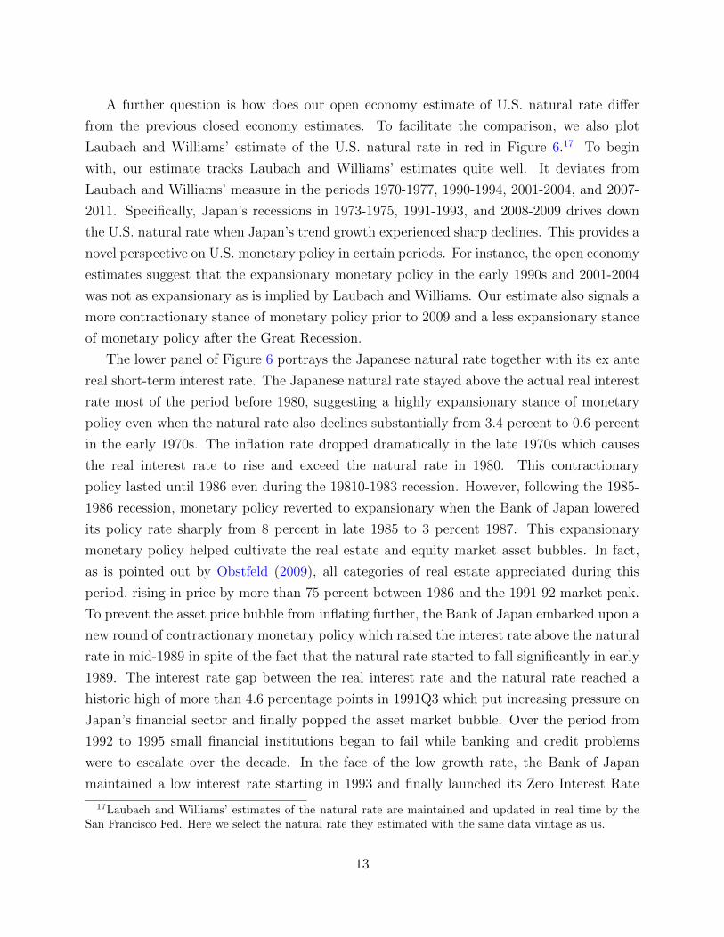
A further question is how does our open economy estimate of U.S. natural rate differ

from the previous closed economy estimates. To facilitate the comparison, we also plot

Laubach and Williams’ estimate of the U.S. natural rate in red in Figure 6.17 To begin

with, our estimate tracks Laubach and Williams’ estimates quite well. It deviates from

Laubach and Williams’ measure in the periods 1970-1977, 1990-1994, 2001-2004, and 2007-

2011. Specifically, Japan’s recessions in 1973-1975, 1991-1993, and 2008-2009 drives down

the U.S. natural rate when Japan’s trend growth experienced sharp declines. This provides a

novel perspective on U.S. monetary policy in certain periods. For instance, the open economy

estimates suggest that the expansionary monetary policy in the early 1990s and 2001-2004

was not as expansionary as is implied by Laubach and Williams. Our estimate also signals a

more contractionary stance of monetary policy prior to 2009 and a less expansionary stance

of monetary policy after the Great Recession.

The lower panel of Figure 6 portrays the Japanese natural rate together with its ex ante

real short-term interest rate. The Japanese natural rate stayed above the actual real interest

rate most of the period before 1980, suggesting a highly expansionary stance of monetary

policy even when the natural rate also declines substantially from 3.4 percent to 0.6 percent

in the early 1970s. The inflation rate dropped dramatically in the late 1970s which causes

the real interest rate to rise and exceed the natural rate in 1980. This contractionary

policy lasted until 1986 even during the 19810-1983 recession. However, following the 1985-

1986 recession, monetary policy reverted to expansionary when the Bank of Japan lowered

its policy rate sharply from 8 percent in late 1985 to 3 percent 1987. This expansionary

monetary policy helped cultivate the real estate and equity market asset bubbles. In fact,

as is pointed out by Obstfeld (2009), all categories of real estate appreciated during this

period, rising in price by more than 75 percent between 1986 and the 1991-92 market peak.

To prevent the asset price bubble from inflating further, the Bank of Japan embarked upon a

new round of contractionary monetary policy which raised the interest rate above the natural

rate in mid-1989 in spite of the fact that the natural rate started to fall significantly in early

1989. The interest rate gap between the real interest rate and the natural rate reached a

historic high of more than 4.6 percentage points in 1991Q3 which put increasing pressure on

Japan’s financial sector and finally popped the asset market bubble. Over the period from

1992 to 1995 small financial institutions began to fail while banking and credit problems

were to escalate over the decade. In the face of the low growth rate, the Bank of Japan

maintained a low interest rate starting in 1993 and finally launched its Zero Interest Rate

17Laubach and Williams’ estimates of the natural rate are maintained and updated in real time by theSan Francisco Fed. Here we select the natural rate they estimated with the same data vintage as us.

13

Policy (ZIRP) in February 1999. Nevertheless, since the natural rate also stayed at a low

level after the 1991-1993 recession, the Zero Interest Rate Policy exerted little expansionary

effect, especially after 2000 when Japan slipped into deflation.18 The Bank of Japan raised

interest rates in 2006. This seems again to have been a policy mistake since the natural rate

turned negative in 2006Q4. The contractionary monetary policy lasted from 2006 to 2014,

even after Japan returned to a zero interest rate policy in 2010, which impeded Japan from

recovering from the 2008-2009 recession and the 2012 recession. In 2013 and 2014, a change

of government was followed by the launch of a program of Qualitative and Quantitative

Easing which finally lowered the real interest rate below the natural rate. Given that the

natural rate stayed negative until the end of our sample, it’s perhaps not so surprising that

the Bank of Japan began to experiment with negative interest rates in 2016.

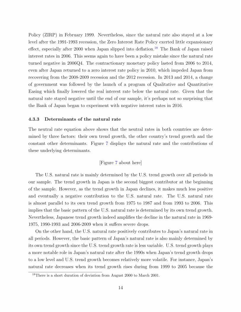
4.3.3 Determinants of the natural rate

The neutral rate equation above shows that the neutral rates in both countries are deter-

mined by three factors: their own trend growth, the other country’s trend growth and the

constant other determinants. Figure 7 displays the natural rate and the contributions of

these underlying determinants.

[Figure 7 about here]

The U.S. natural rate is mainly determined by the U.S. trend growth over all periods in

our sample. The trend growth in Japan is the second biggest contributor at the beginning

of the sample. However, as the trend growth in Japan declines, it makes much less positive

and eventually a negative contribution to the U.S. natural rate. The U.S. natural rate

is almost parallel to its own trend growth from 1975 to 1987 and from 1993 to 2006. This

implies that the basic pattern of the U.S. natural rate is determined by its own trend growth.

Nevertheless, Japanese trend growth indeed amplifies the decline in the natural rate in 1969-

1975, 1990-1993 and 2006-2009 when it suffers severe drops.

On the other hand, the U.S. natural rate positively contributes to Japan’s natural rate in

all periods. However, the basic pattern of Japan’s natural rate is also mainly determined by

its own trend growth since the U.S. trend growth rate is less variable. U.S. trend growth plays

a more notable role in Japan’s natural rate after the 1990s when Japan’s trend growth drops

to a low level and U.S. trend growth becomes relatively more volatile. For instance, Japan’s

natural rate decreases when its trend growth rises during from 1999 to 2005 because the

18There is a short duration of deviation from August 2000 to March 2001.

14

U.S. trend growth decreases at the time. On the other hand, the sustainable U.S. economic

recovery drives up the Japanese natural rate even when Japan’s domestic trend growth stays

at a low level after 2009.

5 Robustness

In the baseline model above, we adopted the exact model specification in Laubach and

Williams (2003) and applied it to our two-country setting. While copying the Laubach and

Williams specification for the United States might seem uncontroversial and even desirable

from the perspective of facilitating the comparison of our results with theirs, it is less obvious

that using their specification for Japan makes sense (although Umino (2014) does essentially

that). There are many dimensions along which we might seek to find a better small scale

statistical model of the U.S. and Japanese economies for the purposes of our exercise, but in

this section we will focus on just one, namely, how the results might be changed if instead

of adapting the Laubach and Williams specification one-for-one, we allow lag lengths in the

IS curve and the Phillips curve for each country to be chosen by some statistical criterion.

[Table 2 about here]

Given the large number of parameters in the full model, it is not feasible to search over all

possible specifications of the IS curves and Phillips curves. Instead, we estimated individual

IS and Phillips curves for each country. For the IS curve, we proxied the output gap with the

deviation of output from its HP-filter smoothed level. Likewise we proxied the interest rate

gap by the deviation of real interest rates from their HP-smoothed level. And for the each

country’s Phillips curve we also proxied the output gap with the deviation of output from its

HP-smoothed level. We then varied the lag length of the lagged output terms in the IS curve

and the lagged inflation terms in the Phillips curve up to eight lags and then computed the

Bayes Information Criterion (BIC) for each specification. The results are shown in Table 2.

There are two points worth noting. First, note that the largest gain in terms of the BIC

comes from going from having no lags to having just one. There is not a lot of difference

in terms of the BIC from having one versus eight lags. We have highlighted in bold the lag

length in each case that minimises the BIC for each equation.

[Table 3 and Figures 8 and 9 about here]

We then used these results to tighten the priors in our estimation as shown in Table 3 and

Figures 8 and 9. Note that the signs and indeed the magnitude of the posterior estimates

15

of almost all of the coefficients are little changed from what we report in Table 1. Figures

10 through 13 show how our estimates of the output gap and the natural rate of interest

change when we use the prior with lag lengths in the IS and Phillips curve chosen using the

BIC. A cursory examination of the figures shows that the results are essentially the same.

[Figures 10 to 13 about here]

Our second robustness check looks at the residuals from the observation equation in

our model, and specifically checks to see if they satisfy the key assumption of normality.

Table 4 reports the p-values of Ljung-Box (LB) and Kolmogorov-Smirnov (KS) tests for

correlation and normality of the residuals from the observation equations of our baseline

model and the robust model estimated using priors with lag lengths selected using the BIC.

Note that in almost all cases both the baseline and the robust model pass both tests at

standard significance levels. We reject the nulls of no serial correlation and normality for

the Japanese Phillips curve in the baseline specification, and also in the robust specification.

We also reject the null of no serial correlation in the robust specification for the U.S. Phillips

curve.

[Table 4 about here]

6 Conclusion

In this paper, we estimate a time-varying natural rate of interest for U.S. and Japan by

Bayesian methods over the period 1961-2014. Our model is a two-country version of the semi-

structural model proposed by Laubach and Williams (2003). We assume perfect risk sharing

and complete international asset markets so that the two countries are linked through a

simple natural rate determination equation. By properly incorporating the prior information,

our estimation avoids the “pile-up” problem suffered by previous estimation of the natural

rate of interest by maximum likelihood methods.

The empirical analysis shows that the natural rate is not only related to the trend growth

in home country but also the trend growth in foreign country. For both U.S. and Japan,

the basic pattern of the natural rate is determined primarily by its own country’s trend

growth of potential output while the other country’s trend growth rate indeed contributes

substantially to the natural rate in home country during several special periods. For instance,

Japan’s trend growth amplifies the decline in U.S. natural rate in 1969-1975, 1990-1993 and

16

2006-2009 when Japanese trend growth experienced sharp decreases. On the other hand, the

recent economic recovery in U.S. also helps driving up the Japanese natural rate after 2009.

As a complement to our study, estimating the natural rate in real time and evaluating the

associated uncertainty when information is incomplete could be done within our framework.

In addition, introducing more countries into the foreign country side would also provide

more appropriate evaluation of the foreign influence on the U.S. natural rate if the data

aggregation problem is properly handled. However, these issues are left for further research.

Supplementary Data

The datasets of this paper (1. code and programs, 2. Data, 3. detailed readme files) are

collected in the electronic supplementary material of this article.

References

Barsky, R., A. Justiniano, and L. Melosi (2014). The natural rate of interest and its usefulness

for monetary policy. The American Economic Review 104 (5), 37–43.

Berger, T. and B. Kempa (2014). Time-varying equilibrium rates in small open economies:

Evidence for canada. Journal of Macroeconomics 39, 203–214.

Bernanke, B. S. (2015). Why are interest rates so low. http://www.brookings.edu/blogs/

ben-bernanke/posts/2015/03/30-why-interest-rates-so-low.

Chudik, A. and R. Straub (2017). Size, openness, and macroeconomic interdependence.

International Economic Review 58 (1), 33–55.

Clarida, R., J. Galı, and M. Gertler (2002). A simple framework for international monetary

policy analysis. Journal of Monetary Economics 49 (5), 879–904.

Clark, T. E. and S. Kozicki (2005). Estimating equilibrium real interest rates in real time.

The North American Journal of Economics and Finance 16 (3), 395–413.

Curdia, V., A. Ferrero, G. C. Ng, and A. Tambalotti (2015). Has us monetary policy tracked

the efficient interest rate? Journal of Monetary Economics 70, 72–83.

Frenkel, J. A. and A. Razin (1986). Fiscal policies in the world economy. Journal of Political

Economy 94 (3, Part 1), 564–594.

17

Holston, K., T. Laubach, and J. C. Williams (2017). Measuring the natural rate of interest:

International trends and determinants. Journal of International Economics .

Laubach, T. and J. C. Williams (2003). Measuring the natural rate of interest. Review of

Economics and Statistics 85 (4), 1063–1070.

Laubach, T. and J. C. Williams (2016). Measuring the natural rate of interest redux. Business

Economics 51 (2), 57–67.

Mesonnier, J.-S. and J.-P. Renne (2007). A time-varying natural rate of interest for the euro

area. European Economic Review 51 (7), 1768–1784.

Obstfeld, M. (2009). Time of troubles: The yen and japan’s economy, 1985-2008. Technical

report, National Bureau of Economic Research.

Pescatori, A. and J. Turunen (2015). Lower for longer: Neutral rates in the united states.

IMF Working Paper 15/135 .

Stock, J. H. (1994). Unit roots, structural breaks and trends. Handbook of econometrics 4,

2739–2841.

Trehan, B. and T. Wu (2007). Time-varying equilibrium real rates and monetary policy

analysis. Journal of Economic dynamics and Control 31 (5), 1584–1609.

Umino, S. (2014). Real-time estimation of the equilibrium real interest rate: Evidence from

japan. The North American Journal of Economics and Finance 28, 17–32.

Wynne, M. and R. Zhang (2016). Measuring the “world” natural rate of interest. Manuscript .

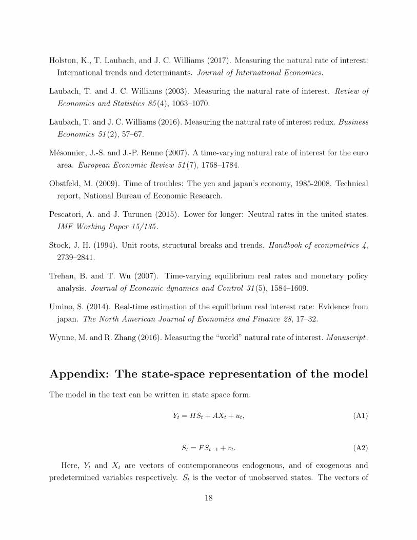
Appendix: The state-space representation of the model

The model in the text can be written in state space form:

Yt = HSt +AXt + ut, (A1)

St = FSt−1 + vt. (A2)

Here, Yt and Xt are vectors of contemporaneous endogenous, and of exogenous and

predetermined variables respectively. St is the vector of unobserved states. The vectors of

18

stochastic disturbance ut and vt are assumed to be Gaussian and mutually uncorrelated with

mean zero and covariance matrices R and Q, respectively.

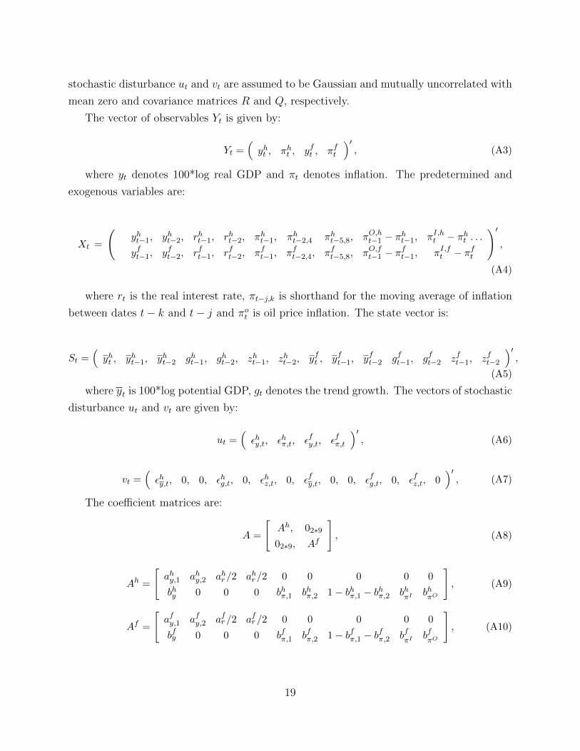
The vector of observables Yt is given by:

Yt =(yht , πht , yft , πft

)′, (A3)

where yt denotes 100*log real GDP and πt denotes inflation. The predetermined and

exogenous variables are:

Xt =

(yht−1, yht−2, rht−1, rht−2, πht−1, πht−2,4 πht−5,8, πO,ht−1 − πht−1, πI,ht − πht . . .yft−1, yft−2, rft−1, rft−2, πft−1, πft−2,4, πft−5,8, πO,ft−1 − π

ft−1, πI,ft − π

ft

)′,

(A4)

where rt is the real interest rate, πt−j,k is shorthand for the moving average of inflation

between dates t− k and t− j and πot is oil price inflation. The state vector is:

St =(yht , yht−1, yht−2 ght−1, ght−2, zht−1, zht−2, yft , yft−1, yft−2 gft−1, gft−2 zft−1, zft−2

)′,

(A5)

where yt is 100*log potential GDP, gt denotes the trend growth. The vectors of stochastic

disturbance ut and vt are given by:

ut =(εhy,t, εhπ,t, εfy,t, εfπ,t

)′, (A6)

vt =(εhy,t, 0, 0, εhg,t, 0, εhz,t, 0, εfy,t, 0, 0, εfg,t, 0, εfz,t, 0

)′, (A7)

The coefficient matrices are:

A =

[Ah, 02∗9

02∗9, Af

], (A8)

Ah =

[ahy,1 ahy,2 ahr/2 ahr/2 0 0 0 0 0

bhy 0 0 0 bhπ,1 bhπ,2 1− bhπ,1 − bhπ,2 bhπI

bhπO

], (A9)

Af =

[afy,1 afy,2 afr/2 afr/2 0 0 0 0 0

bfy 0 0 0 bfπ,1 bfπ,2 1− bfπ,1 − bfπ,2 bf

πIbfπO

], (A10)

19

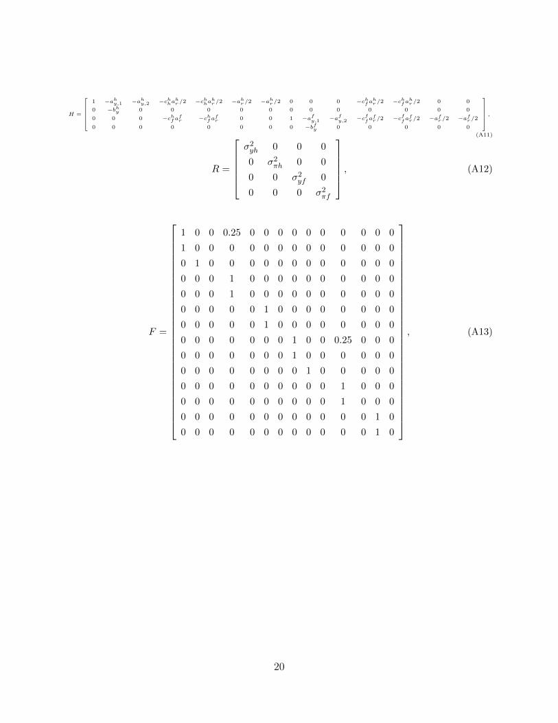
H =

1 −ahy,1 −ahy,2 −chha

hr /2 −chha

hr /2 −ahr /2 −ahr /2 0 0 0 −chf a

hr /2 −chf a

hr /2 0 0

0 −bhy 0 0 0 0 0 0 0 0 0 0 0 0

0 0 0 −chf afr −chf a

fr 0 0 1 −afy,1 −afy,2 −cf

fafr /2 −cf

fafr /2 −afr /2 −afr /2

0 0 0 0 0 0 0 0 −bfy 0 0 0 0 0

,(A11)

R =

σ2yh 0 0 0

0 σ2πh 0 0

0 0 σ2yf 0

0 0 0 σ2πf

, (A12)

F =

1 0 0 0.25 0 0 0 0 0 0 0 0 0 0

1 0 0 0 0 0 0 0 0 0 0 0 0 0

0 1 0 0 0 0 0 0 0 0 0 0 0 0

0 0 0 1 0 0 0 0 0 0 0 0 0 0

0 0 0 1 0 0 0 0 0 0 0 0 0 0

0 0 0 0 0 1 0 0 0 0 0 0 0 0

0 0 0 0 0 1 0 0 0 0 0 0 0 0

0 0 0 0 0 0 0 1 0 0 0.25 0 0 0

0 0 0 0 0 0 0 1 0 0 0 0 0 0

0 0 0 0 0 0 0 0 1 0 0 0 0 0

0 0 0 0 0 0 0 0 0 0 1 0 0 0

0 0 0 0 0 0 0 0 0 0 1 0 0 0

0 0 0 0 0 0 0 0 0 0 0 0 1 0

0 0 0 0 0 0 0 0 0 0 0 0 1 0

, (A13)

20

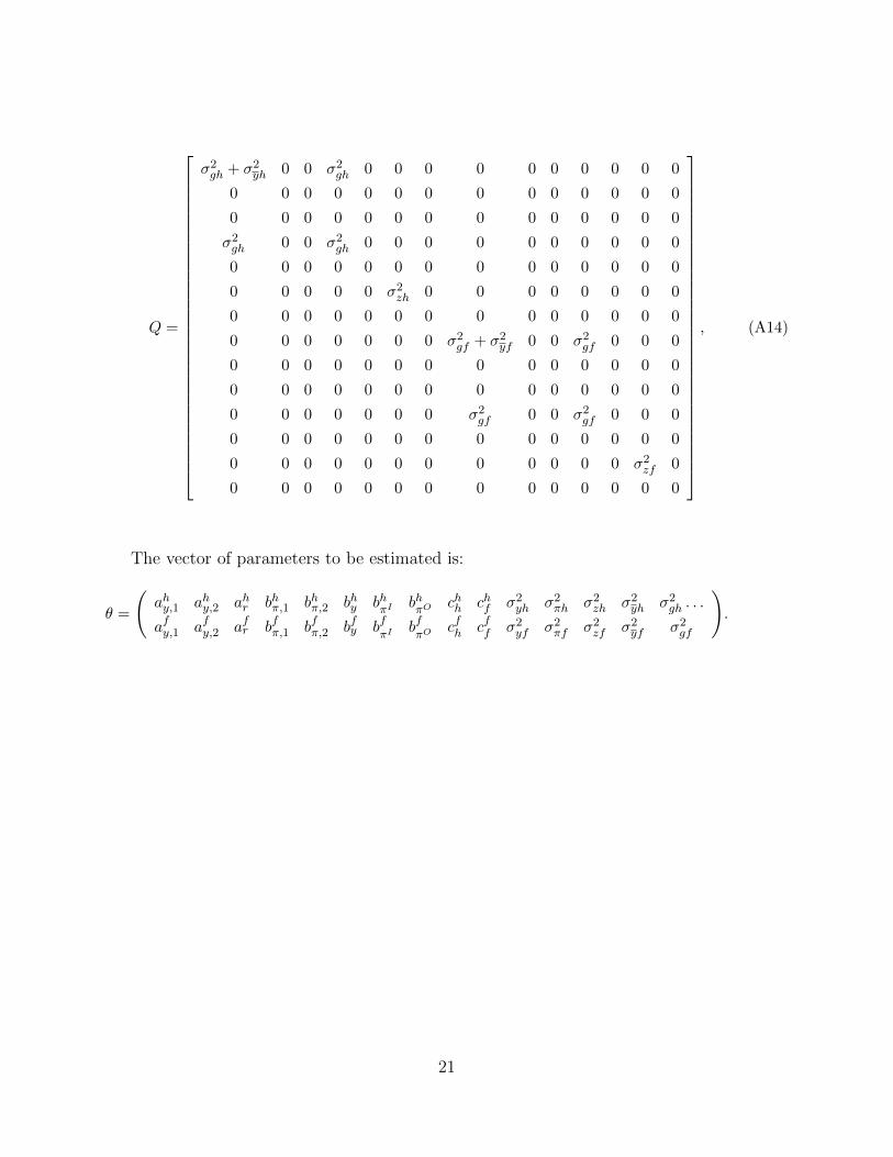
Q =

σ2gh + σ2yh 0 0 σ2gh 0 0 0 0 0 0 0 0 0 0

0 0 0 0 0 0 0 0 0 0 0 0 0 0

0 0 0 0 0 0 0 0 0 0 0 0 0 0

σ2gh 0 0 σ2gh 0 0 0 0 0 0 0 0 0 0

0 0 0 0 0 0 0 0 0 0 0 0 0 0

0 0 0 0 0 σ2zh 0 0 0 0 0 0 0 0

0 0 0 0 0 0 0 0 0 0 0 0 0 0

0 0 0 0 0 0 0 σ2gf + σ2yf 0 0 σ2gf 0 0 0

0 0 0 0 0 0 0 0 0 0 0 0 0 0

0 0 0 0 0 0 0 0 0 0 0 0 0 0

0 0 0 0 0 0 0 σ2gf 0 0 σ2gf 0 0 0

0 0 0 0 0 0 0 0 0 0 0 0 0 0

0 0 0 0 0 0 0 0 0 0 0 0 σ2zf 0

0 0 0 0 0 0 0 0 0 0 0 0 0 0

, (A14)

The vector of parameters to be estimated is:

θ =

(ahy,1 ahy,2 ahr bhπ,1 bhπ,2 bhy bh

πIbhπO

chh chf σ2yh σ2πh σ2zh σ2yh σ2gh . . .

afy,1 afy,2 afr bfπ,1 bfπ,2 bfy bfπI

bfπO

cfh cff σ2yf σ2πf σ2zf σ2yf σ2gf

).

21

1960 1970 1980 1990 2000 2010

0

2

4

6

8

10

12

14

16

18

20

22

Year

Ten

−ye

ar g

over

nmen

t bon

d yi

elds

for

G7

coun

trie

s, %

CanadaFranceGermanyItalyJapanUnited KingdomUnited States

Figure 1: Ten-year government bond yields in G7 countries

22

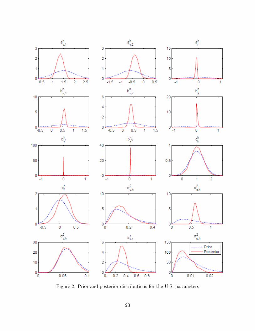
Figure 2: Prior and posterior distributions for the U.S. parameters

23

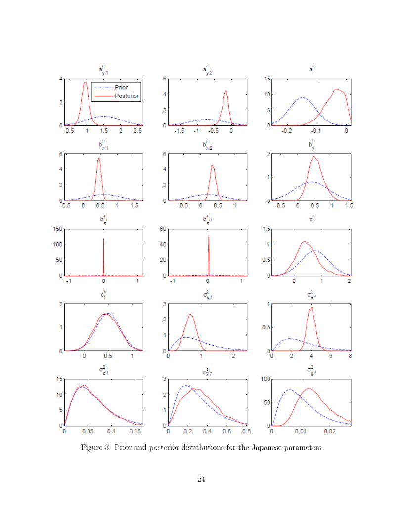
Figure 3: Prior and posterior distributions for the Japanese parameters

24

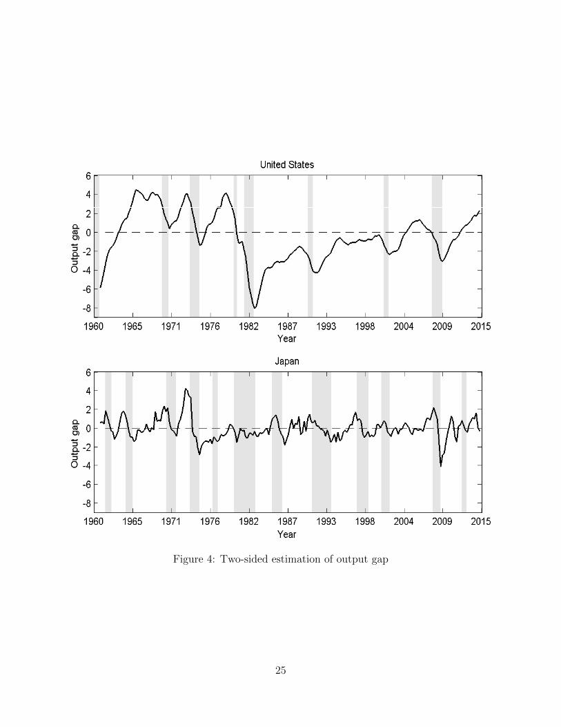
Figure 4: Two-sided estimation of output gap

25

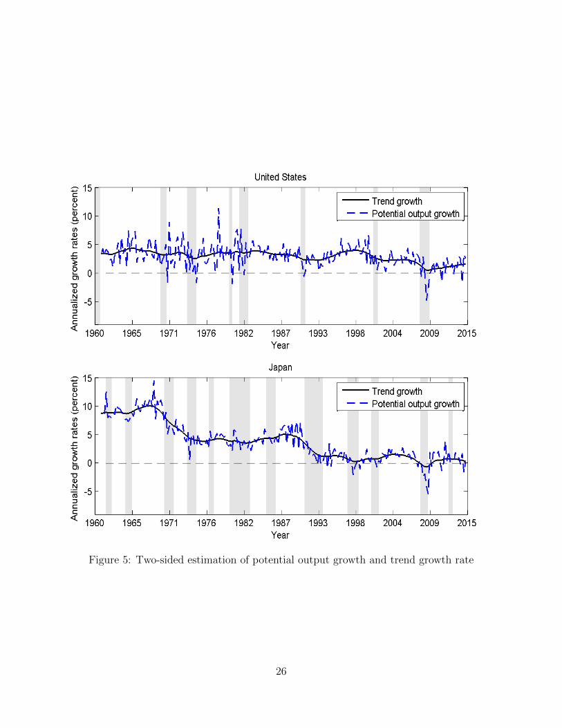
Figure 5: Two-sided estimation of potential output growth and trend growth rate

26

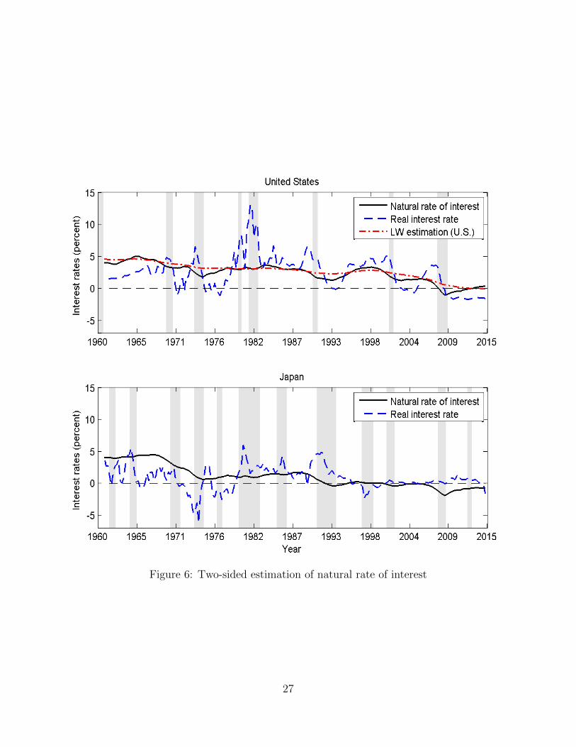
Figure 6: Two-sided estimation of natural rate of interest

27

Figure 7: Natural rate components

28

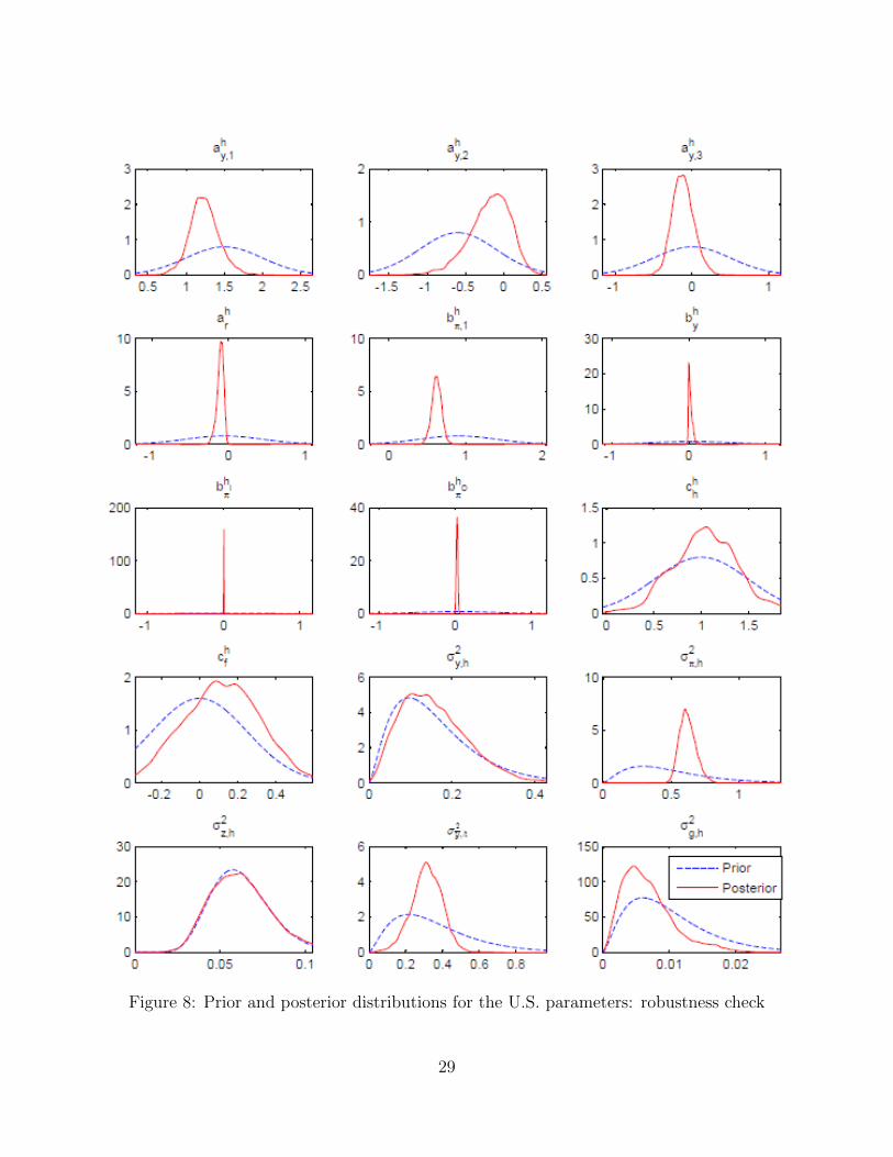
Figure 8: Prior and posterior distributions for the U.S. parameters: robustness check

29

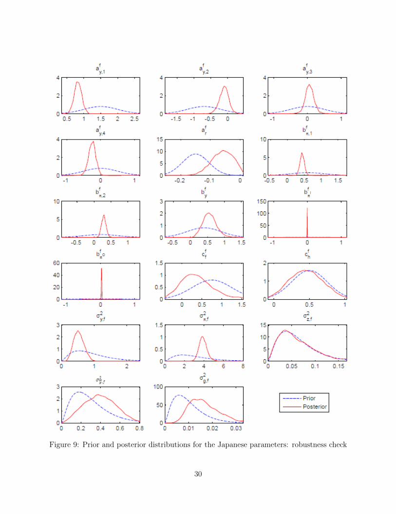
Figure 9: Prior and posterior distributions for the Japanese parameters: robustness check

30

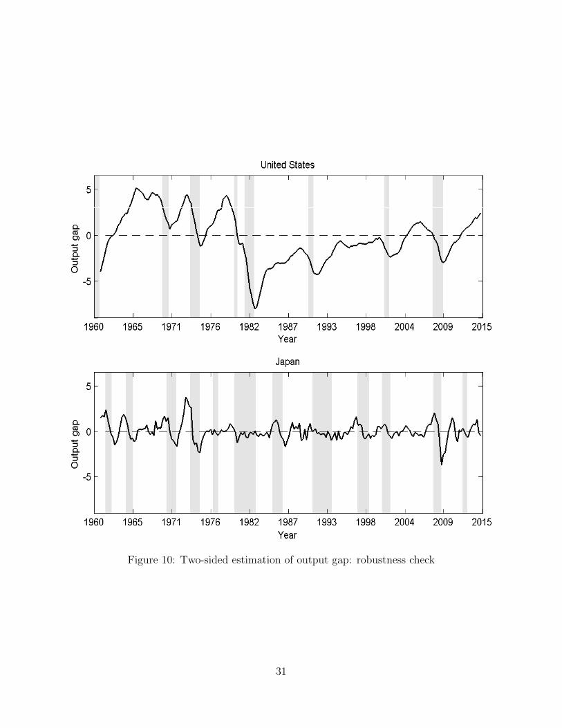
Figure 10: Two-sided estimation of output gap: robustness check

31

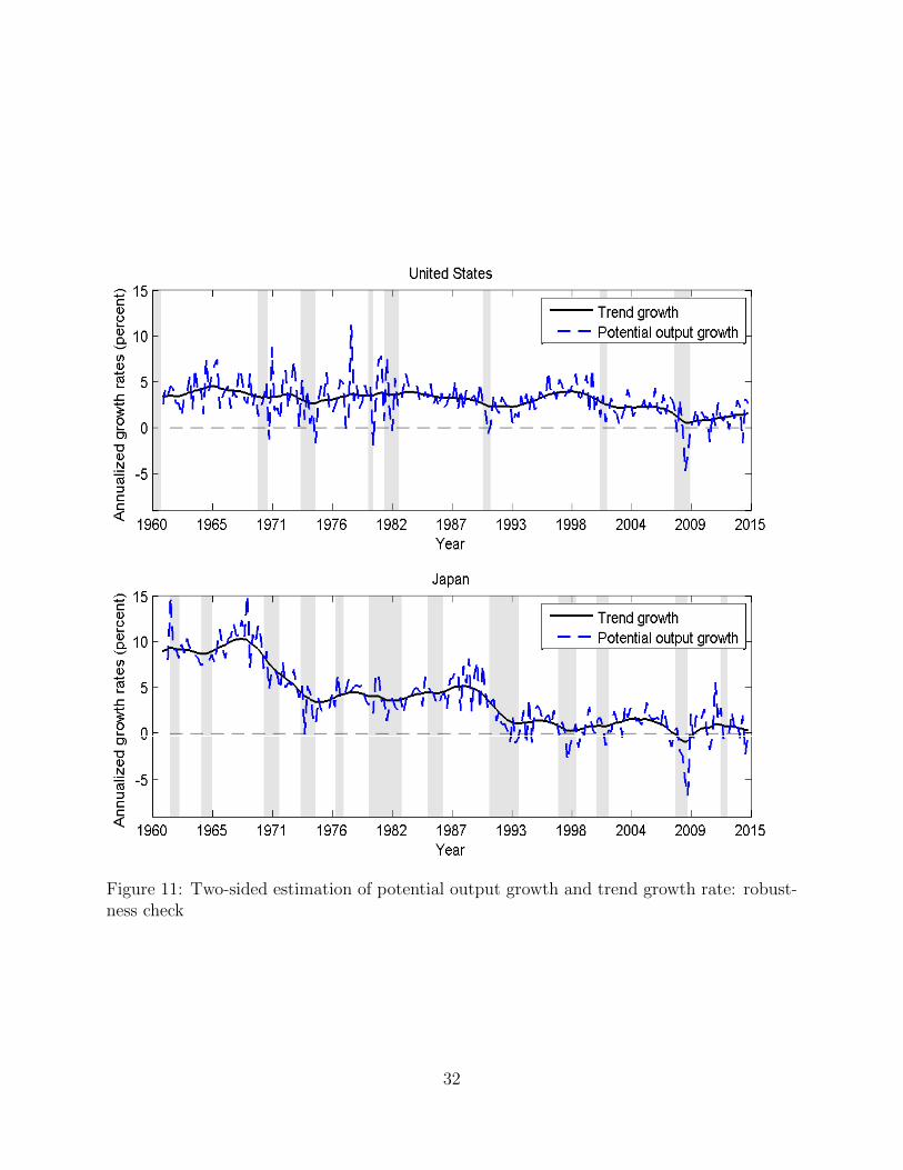
Figure 11: Two-sided estimation of potential output growth and trend growth rate: robust-ness check

32

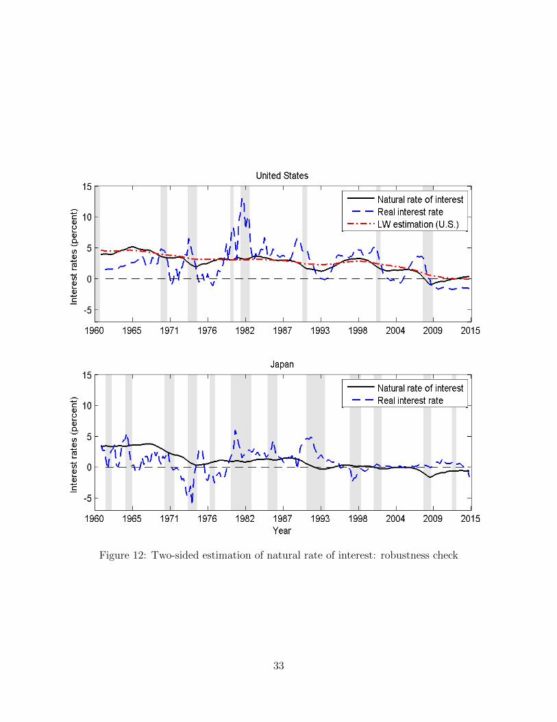
Figure 12: Two-sided estimation of natural rate of interest: robustness check

33

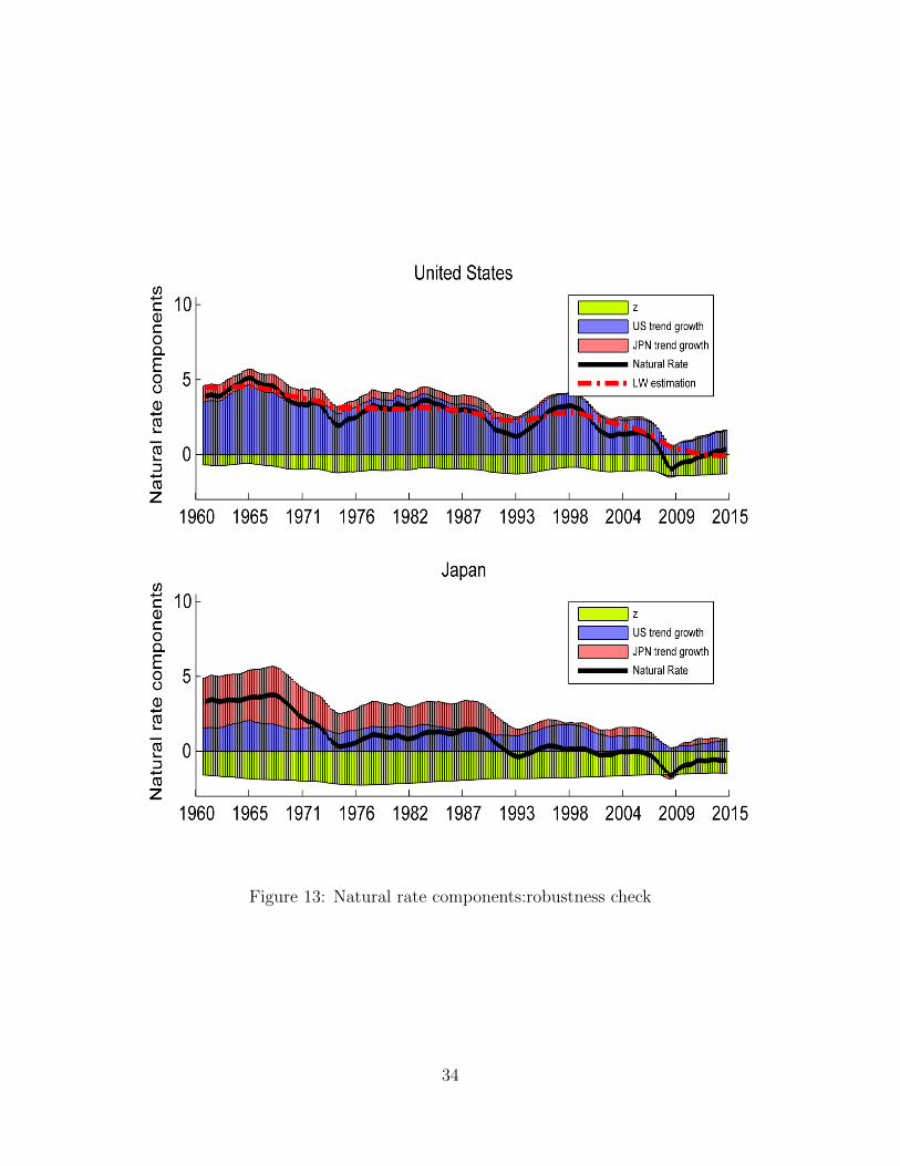
Figure 13: Natural rate components:robustness check

34

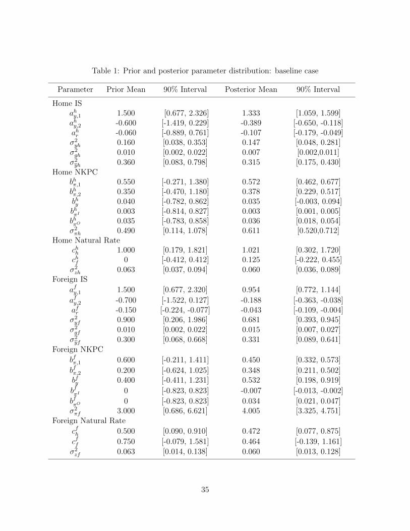
Table 1: Prior and posterior parameter distribution: baseline case

Parameter Prior Mean 90% Interval Posterior Mean 90% Interval

Home ISahy,1 1.500 [0.677, 2.326] 1.333 [1.059, 1.599]ahy,2 -0.600 [-1.419, 0.229] -0.389 [-0.650, -0.118]ahr -0.060 [-0.889, 0.761] -0.107 [-0.179, -0.049]σ2yh 0.160 [0.038, 0.353] 0.147 [0.048, 0.281]σ2gh 0.010 [0.002, 0.022] 0.007 [0.002,0.011]σ2yh 0.360 [0.083, 0.798] 0.315 [0.175, 0.430]

Home NKPCbhπ,1 0.550 [-0.271, 1.380] 0.572 [0.462, 0.677]bhπ,2 0.350 [-0.470, 1.180] 0.378 [0.229, 0.517]bhy 0.040 [-0.782, 0.862] 0.035 [-0.003, 0.094]bhπI 0.003 [-0.814, 0.827] 0.003 [0.001, 0.005]bhπO 0.035 [-0.783, 0.858] 0.036 [0.018, 0.054]σ2πh 0.490 [0.114, 1.078] 0.611 [0.520,0.712]

Home Natural Ratechh 1.000 [0.179, 1.821] 1.021 [0.302, 1.720]chf 0 [-0.412, 0.412] 0.125 [-0.222, 0.455]σ2zh 0.063 [0.037, 0.094] 0.060 [0.036, 0.089]

Foreign IS

afy,1 1.500 [0.677, 2.320] 0.954 [0.772, 1.144]

afy,2 -0.700 [-1.522, 0.127] -0.188 [-0.363, -0.038]afr -0.150 [-0.224, -0.077] -0.043 [-0.109, -0.004]σ2yf 0.900 [0.206, 1.986] 0.681 [0.393, 0.945]σ2gf 0.010 [0.002, 0.022] 0.015 [0.007, 0.027]σ2yf 0.300 [0.068, 0.668] 0.331 [0.089, 0.641]

Foreign NKPC

bfπ,1 0.600 [-0.211, 1.411] 0.450 [0.332, 0.573]

bfπ,2 0.200 [-0.624, 1.025] 0.348 [0.211, 0.502]bfy 0.400 [-0.411, 1.231] 0.532 [0.198, 0.919]

bfπI

0 [-0.823, 0.823] -0.007 [-0.013, -0.002]

bfπO

0 [-0.823, 0.823] 0.034 [0.021, 0.047]σ2πf 3.000 [0.686, 6.621] 4.005 [3.325, 4.751]

Foreign Natural Rate

cfh 0.500 [0.090, 0.910] 0.472 [0.077, 0.875]

cff 0.750 [-0.079, 1.581] 0.464 [-0.139, 1.161]

σ2zf 0.063 [0.014, 0.138] 0.060 [0.013, 0.128]

35

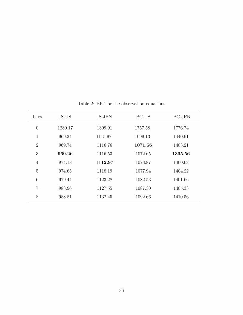
Table 2: BIC for the observation equations

Lags IS-US IS-JPN PC-US PC-JPN

0 1280.17 1309.91 1757.58 1776.74

1 969.34 1115.97 1099.13 1440.91

2 969.74 1116.76 1071.56 1403.21

3 969.26 1116.53 1072.65 1395.56

4 974.18 1112.97 1073.87 1400.68

5 974.65 1118.19 1077.94 1404.22

6 979.44 1123.28 1082.53 1401.66

7 983.96 1127.55 1087.30 1405.33

8 988.81 1132.45 1092.66 1410.56

36

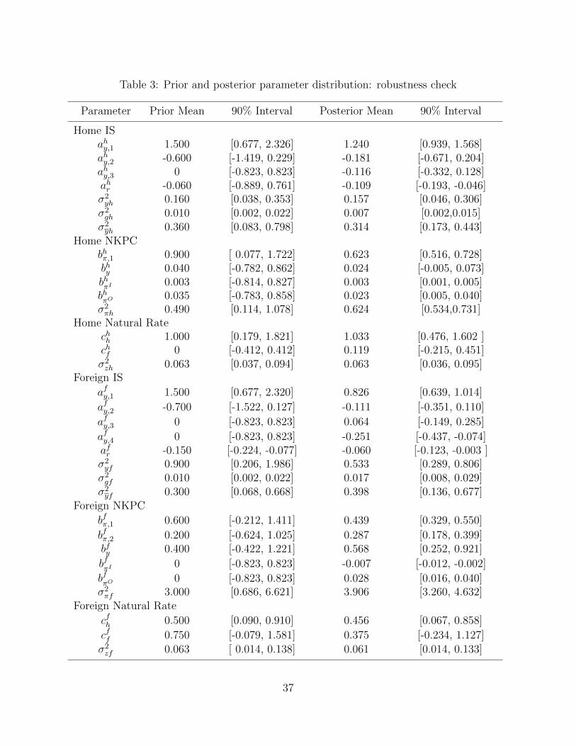
Table 3: Prior and posterior parameter distribution: robustness check

Parameter Prior Mean 90% Interval Posterior Mean 90% Interval

Home ISahy,1 1.500 [0.677, 2.326] 1.240 [0.939, 1.568]ahy,2 -0.600 [-1.419, 0.229] -0.181 [-0.671, 0.204]ahy,3 0 [-0.823, 0.823] -0.116 [-0.332, 0.128]ahr -0.060 [-0.889, 0.761] -0.109 [-0.193, -0.046]σ2yh 0.160 [0.038, 0.353] 0.157 [0.046, 0.306]σ2gh 0.010 [0.002, 0.022] 0.007 [0.002,0.015]σ2yh 0.360 [0.083, 0.798] 0.314 [0.173, 0.443]

Home NKPCbhπ,1 0.900 [ 0.077, 1.722] 0.623 [0.516, 0.728]bhy 0.040 [-0.782, 0.862] 0.024 [-0.005, 0.073]bhπI 0.003 [-0.814, 0.827] 0.003 [0.001, 0.005]bhπO 0.035 [-0.783, 0.858] 0.023 [0.005, 0.040]σ2πh 0.490 [0.114, 1.078] 0.624 [0.534,0.731]

Home Natural Ratechh 1.000 [0.179, 1.821] 1.033 [0.476, 1.602 ]chf 0 [-0.412, 0.412] 0.119 [-0.215, 0.451]σ2zh 0.063 [0.037, 0.094] 0.063 [0.036, 0.095]

Foreign IS

afy,1 1.500 [0.677, 2.320] 0.826 [0.639, 1.014]

afy,2 -0.700 [-1.522, 0.127] -0.111 [-0.351, 0.110]

afy,3 0 [-0.823, 0.823] 0.064 [-0.149, 0.285]

afy,4 0 [-0.823, 0.823] -0.251 [-0.437, -0.074]afr -0.150 [-0.224, -0.077] -0.060 [-0.123, -0.003 ]σ2yf 0.900 [0.206, 1.986] 0.533 [0.289, 0.806]σ2gf 0.010 [0.002, 0.022] 0.017 [0.008, 0.029]σ2yf 0.300 [0.068, 0.668] 0.398 [0.136, 0.677]

Foreign NKPC

bfπ,1 0.600 [-0.212, 1.411] 0.439 [0.329, 0.550]

bfπ,2 0.200 [-0.624, 1.025] 0.287 [0.178, 0.399]bfy 0.400 [-0.422, 1.221] 0.568 [0.252, 0.921]

bfπI

0 [-0.823, 0.823] -0.007 [-0.012, -0.002]

bfπO

0 [-0.823, 0.823] 0.028 [0.016, 0.040]σ2πf 3.000 [0.686, 6.621] 3.906 [3.260, 4.632]

Foreign Natural Rate

cfh 0.500 [0.090, 0.910] 0.456 [0.067, 0.858]

cff 0.750 [-0.079, 1.581] 0.375 [-0.234, 1.127]

σ2zf 0.063 [ 0.014, 0.138] 0.061 [0.014, 0.133]

37

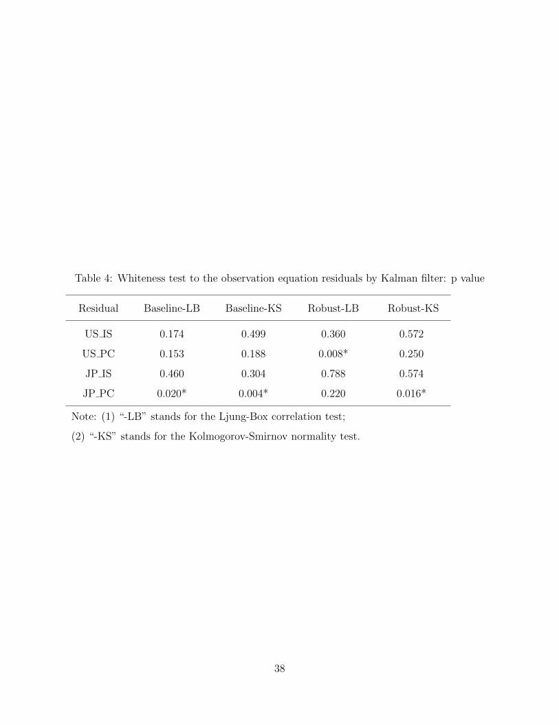
Table 4: Whiteness test to the observation equation residuals by Kalman filter: p value

Residual Baseline-LB Baseline-KS Robust-LB Robust-KS

US IS 0.174 0.499 0.360 0.572

US PC 0.153 0.188 0.008* 0.250

JP IS 0.460 0.304 0.788 0.574

JP PC 0.020* 0.004* 0.220 0.016*

Note: (1) “-LB” stands for the Ljung-Box correlation test;

(2) “-KS” stands for the Kolmogorov-Smirnov normality test.

38