ISSN 1084-1695

Aging Studies Program Paper No. 18

Estimating the Income Effecton Retirement

Douglas Holtz-Eakin, David Joulfaianand Harvey S. Rosen

Maxwell Center for Demography and Economics of Aging

Center for Policy ResearchMaxwell School of Citizenship and Public Affairs

Syracuse UniversitySyracuse, New York 13244-1020

April 1999

Support for the Aging Studies Program Series is provided by grant numberP20-AG12837 from the National Institute on Aging.

ii

Abstract

One of the most important issues in the debate over Social Security is how various changes

in the system would change retirement behavior. A critical parameter in this context is the income

effect on retirement— how a change in income affects retirement behavior, ceteris paribus. To

estimate the income effect, we examine tax-return generated data on the labor force activity of a

group of older people before and after they receive inheritances. The results are consistent with the

notion that income effects are small. Neither retirement decisions nor the magnitude of earnings

conditional on working seem to be affected very much by the receipt of an inheritance.

Center for Policy ResearchTim Smeeding, Director

Richard V. Burkhauser, Associate Director for Aging Studies

Center for Demography and Economics of AgingDouglas A. Wolf, Director

The Maxwell Center for Demography and Economics of Aging was established in September 1994 withcore funding from the National Institute on Aging (Grant No. P20-AG12837). The goals of the Centerare to coordinate and support research activities in aging, publish findings and policy analyses, andconvene workshops, seminars, and conferences intended to train data users and disseminate researchfindings and their implications to the research and policy communities.

The Center produces two paper series, the Aging Studies Paper Series and Papers in Microsimulation.

Many Center publications are available via Adobe Acrobat format. To access these resources attach toour World-Wide Web home page at http://www-cpr.maxwell.syr.edu.

For more information contact: Martha Bonney (mbonney@maxwell.syr.edu).

Center for Policy Research426 Eggers Hall

Syracuse UniversitySyracuse, New York 13244-1020

(315) 443 3114

FAX: (315) 443 1081

1. Introduction

One of the most important issues in the debate over Social Security is how various changes

in the system would affect retirement behavior. This question has been addressed by a very large

empirical literature. (See the review by Lumsdaine and Mitchell 1998.) A typical approach is to

examine the differences in labor force participation among individuals who have different Social

Security benefits, using either cross-sectional, time series, or panel data. A couple of important

practical problems are associated with this strategy. First, the investigator may not know individuals’

actual Social Security benefits; they generally have to be estimated on the basis of (possibly

incomplete) data on earnings history, marital status, and so forth. Second, Social Security benefits

may be endogenous— benefits are tied to past earnings, and unobserved differences across individuals

in their past work behavior may be correlated with their current labor force decisions. Put differently,

it is very difficult to locate well measured, exogenous differences in retirement benefits. Hence, there

is still a great deal of disagreement on how various changes in Social Security would affect retirement

behavior.

Although the decision to retire is in principle very complicated, it is useful to think about the

problem in terms of the simplest model of leisure-consumption choice. In that setting, the effect of1

a change in a worker’s incentives depends on an income effect and a substitution effect. Our focus

in this paper is on the latter— how an exogenous change in income affects retirement decisions. To

the extent that various reform proposals involve changes in potential retirees’ incomes, then knowing

the magnitude of the income effect is central to assessing the impacts of such proposals. And even

when policies change the net wage associated with working, the usual Slutsky decomposition tells

us that the income effect in part determines the impact on labor supply decisions. In a similar spirit,

assessing the efficiency consequences of Social Security, tax, or other government policies generally

require analyses to separate the substitution effects and income effects on labor supply.

-2-

A key part of the empirical strategy suggested by this agenda is finding plausibly exogenous

changes in the income or wealth of older individuals that can be used to determine the effect of the

change in income or wealth on retirement probabilities, ceteris paribus. For example, Krueger and

Pischke (1992) examined an exogenous change in Social Security benefits that involved one group

of retirees (the “notch babies”) and not others. By comparing retirement behavior of the two groups,

Krueger and Pischke were able to infer the impact of changes in Social Security wealth upon

retirement probabilities. They found that, ceteris paribus, changes in the magnitude of Social

Security wealth are statistically insignificant. Similarly, Neumark and Powers (1998) took advantage

of state-by-state differences in the generosity of benefits for Supplemental Security Income (SSI) to

estimate this program’s impact on the labor supply effects of older men who are not yet eligible for

Social Security. They found that SSI has a modest impact on the labor supply and earnings of this

subset of the older population, suggesting that an income effect is present.

The Krueger-Pischke and Neumark-Powers papers illustrate the difficulty of finding

exogenous changes within the context of the modern Social Security system. Two important

historical studies have sought to estimate income effects on retirement using earlier programs that

provide more suitable “natural experiments.” Friedberg (1998) analyzed data from the 1940 and 1950

censuses to estimate how retirement decisions varied with differences in benefits received from Old

Age Assistance (OAA), a now defunct federal transfer program. Importantly, OAA benefits varied

by state, affording a source of exogenous variation. An even earlier historical episode was studied

by Costa (1995), who analyzed the effect of pensions on the retirement decisions of Civil War

veterans. Veterans of the Union Army were eligible for a pension regardless of labor force

participation and regardless of current or past income. The amount depended only on their health

status and whether any disabilities could be linked to the war.

-3-

Both Friedberg and Costa found substantial income effects. Friedberg estimated an elasticity

of labor force nonparticipation with respect to retirement income ranging from 0.25 to 0.40,

depending on the specification. Costa found a nonparticipation elasticity of 0.73. In their review of

a number of historical studies, Pope and Wimmer (1998, p. 219) concluded that “at the turn of the

century there existed a strong relationship between income and retirement” but that “the importance

of current income or wage upon the retirement decision has been declining over time.”

This paper brings a unique— and more modern— data set to bear on the problem of measuring

the income effects associated with retirement behavior. The sample consists of the 1982 and 1985

federal individual income tax returns of a group of older people who received inheritances in 1982

and 1983, along with information about the size of their inheritances. Tax return data in 1982 and2

1985 allow us to compute how many members in the household were participating in the labor force

in each year. We examine their transitions into and out of the labor force between 1982 and 1985,

and the effect of the size of inheritances upon these transitions. This allows us to infer the income

effect on the probability that a single individual, or one or both members of a married couple, retires.

The data and empirical strategy are described in Section 2. Section 3 presents the results,

which are consistent with the notion that income effects are small. Neither the retirement decision

nor earnings conditional on working seem to be altered very much by the receipt of an inheritance.

Section 4 concludes with a summary and suggestions for future research.

2. Data and Empirical Strategy

Construction of our data set began with an Internal Revenue Service (IRS) sample of estate

tax records. The IRS selected a 1 percent sample of estate tax returns of people who died in 1982

and whose estate tax returns were filed in 1982 and 1983. In addition, returns with total assets over

-4-

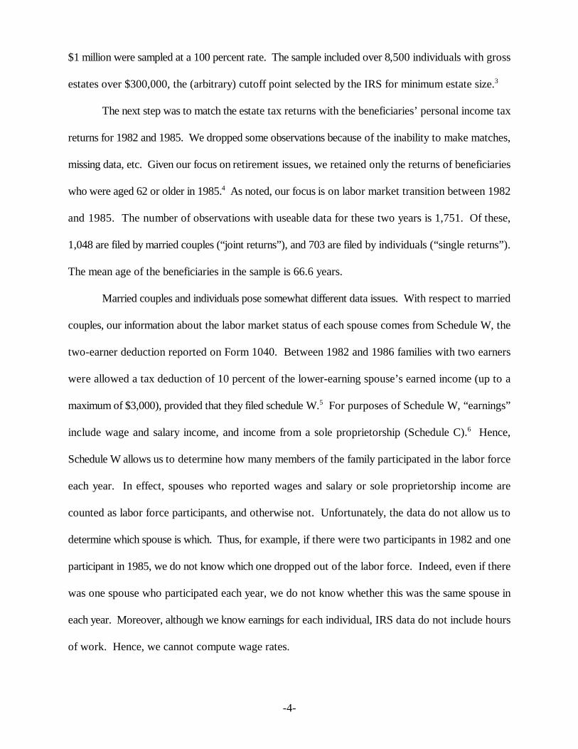
$1 million were sampled at a 100 percent rate. The sample included over 8,500 individuals with gross

estates over $300,000, the (arbitrary) cutoff point selected by the IRS for minimum estate size.3

The next step was to match the estate tax returns with the beneficiaries’ personal income tax

returns for 1982 and 1985. We dropped some observations because of the inability to make matches,

missing data, etc. Given our focus on retirement issues, we retained only the returns of beneficiaries

who were aged 62 or older in 1985. As noted, our focus is on labor market transition between 19824

and 1985. The number of observations with useable data for these two years is 1,751. Of these,

1,048 are filed by married couples (“joint returns”), and 703 are filed by individuals (“single returns”).

The mean age of the beneficiaries in the sample is 66.6 years.

Married couples and individuals pose somewhat different data issues. With respect to married

couples, our information about the labor market status of each spouse comes from Schedule W, the

two-earner deduction reported on Form 1040. Between 1982 and 1986 families with two earners

were allowed a tax deduction of 10 percent of the lower-earning spouse’s earned income (up to a

maximum of $3,000), provided that they filed schedule W. For purposes of Schedule W, “earnings”5

include wage and salary income, and income from a sole proprietorship (Schedule C). Hence,6

Schedule W allows us to determine how many members of the family participated in the labor force

each year. In effect, spouses who reported wages and salary or sole proprietorship income are

counted as labor force participants, and otherwise not. Unfortunately, the data do not allow us to

determine which spouse is which. Thus, for example, if there were two participants in 1982 and one

participant in 1985, we do not know which one dropped out of the labor force. Indeed, even if there

was one spouse who participated each year, we do not know whether this was the same spouse in

each year. Moreover, although we know earnings for each individual, IRS data do not include hours

of work. Hence, we cannot compute wage rates.

-5-

For single returns, we classify those individuals who report wage and salary or sole

proprietorship income as being in the labor force. Here we have no problems in matching the relevant

actor to his or her earnings and age. Again, however, hours of work and wage rates are unknown

to us.

These considerations suggest that it would be futile to attempt to specify a structural

retirement model along the lines of, for example, Rust and Phelan (1997). Such an approach requires

data on each person’s potential wage rate, Social Security benefits, health status, and various

demographic variables. In our data set, we cannot calculate wage rates because we have no

information on hours worked, and even if we could calculate wage rates, we could not match them

to the correct individuals on joint returns. Similarly, we have no information on actual or potential

Social Security benefits.

Given these limitations, we choose a more modest approach that is tailored to the strengths

of our data. To begin, we divide the sample into three groups based on the size of inheritance. For

each inheritance group we construct a transition matrix that shows how the number of earners in the

family (zero, one, or two for joint returns; zero or one for single returns) changes between 1982 and

1985. We then make inferences about income effects by examining the transition matrices to see

whether they differ, and if so, how. Clearly, a concern is that other variables may affect labor supply

differentially among the three groups. If so, one cannot interpret the results as reflecting the

independent effects of inheritance. Therefore, we examine the robustness of our results via some

simple multivariate analyses of retirement decisions.

-6-

3. Results

In this section, we focus first on how transition probabilities for retirement vary with the size

of inheritance. We then turn to a multivariate analysis of the retirement decision.7

Transition Matrices

The results for single returns are found in Table 1. It consists of three transition matrices, one

each for inheritances under $25,000, inheritances between $25,000 and $150,000, and inheritances

greater than $150,000. Each row shows the number of labor force participants in 1982, the columns8

show the number in 1985. Within each cell, the first figure is the number of observations in that cell.

The second figure is the proportion of observations in the corresponding row that fall in the cell. The

figure in parentheses is the associated standard error. Thus, for example, the element in the second

row and first column of the first matrix tells us that 61 of the single individuals in our sample with

inheritances below $25,000 went from being in the labor force in 1982 to not being in the labor force

in 1985, and that these 61 individuals represent 31.9 percent of all the individuals in this group who

were in the labor force in 1982.

Is there an inheritance-induced income effect on retirement? According to Table 1, 31.9

percent of the individuals in the low inheritance group exited the labor force between 1982 and 1985;

47.1 percent of the middle group were out by 1985; and 41.3 percent of the high inheritance group

were out of the labor force in 1985. (See the second rows of the matrices in Table 1.) This almost

50 percent rise as we move from the low to the high inheritance groups is consistent with the

presence of income effects on retirement probabilities. However, these differences are not uniformly

statistically significant. For example, the chi-square test statistic (with two degrees of freedom) for

the null hypothesis that the transition probabilities are identical is 6.34, while the critical value at the

0.05 level is 5.99. However, pairwise comparisons of the transition probabilities for the, middle

-7-

versus high groups and low versus high groups indicate that the differences are not statistically

significant, while the difference between the low and middle group is statistically significant.

To the extent that income effects are present, we would also expect that individuals who are

initially out of the labor force would have a lower probability of entering the labor force the greater

their inheritance, ceteris paribus. Taken at face value, the results in Table 1 are at odds with this

notion— the probability of entering the labor force between 1982 and 1985 actually rises from 1.8

percent in the lowest inheritance group to 4.5 percent in the highest. But the increase is based on

very few observations. Perhaps the key lesson to be learned here is that the response to inheritance9

might very well depend on one’s initial labor force status.

For completeness, we also tested the hypothesis that entire transition matrices (not just

individual cells) are the same. The associated chi-square statistic is 15.2 with 6 degrees of freedom,

which is statistically significant at the 1.8 percent level. This result is driven by the differences among

individuals who were initially in the labor force.

We next consider the corresponding results for joint returns, which are presented in Table 2.

Consider first families that had one earner in 1982. In the low inheritance group, 30.0 percent of

these earners were out of the labor force in 1985; in the middle group 35.5 percent were out in 1985;

and in the high inheritance group 36.5 percent were out of the labor force in 1985. Thus, the10

greater the inheritance, the greater the propensity to go from a one-earner family to a family with no

one in the labor force. Next consider families with two earners in 1982. As we move from low to

medium inheritance groups, the percentage in which both earners opt out of the labor force is roughly

unchanged (7.5 versus 7.0 percent), before rising sharply to 29.3 percent in the high inheritance

group. The percentage in which labor force participation falls from two members to one member

increases from 36.2 percent to 36.8 percent, before rising to 39.0 percent.

-8-

A consistent story appears to emerge— higher inheritances are associated with a greater

propensity to retire. Further, as with the single returns, some (but not all) of the cell proportions are

statistically different from each other in pairwise comparisons. For example, in comparisons of

returns with two earners in 1982, the transition probability to zero labor force participation is

significantly different between the middle and high inheritance groups, and also between the low and

high inheritance groups, but not between the low and middle inheritance groups. Broadening the

focus slightly, we can examine differences conditional on the number of workers in the labor force

in 1982. Specifically, we test whether the second rows in each table are the same. The null

hypothesis that the labor force behavior of one-earner families in 1982 is independent of inheritance

is not rejected by a chi-square test— the test statistic is 2.26 with 4 degrees of freedom. Turning to

the third rows, the corresponding test for two-earner families in 1982 is 16.9 with 4 degrees of

freedom, which is significant at the 1.0 percent level.

As noted earlier, in the presence of income effects, the propensity to enter the labor force

should decline as inheritance increases. The point estimates in Table 2 do not provide much evidence

for this view. The transition rate from one-earner to two-earner households is lower in the top

inheritance group than in the bottom group, but the fall is not monotonic. Further, the point estimates

of the transition from zero-earner to one-earner households increase with inheritance. However, not

all of the differences are statistically significant on a pairwise basis.

As in the case of single earners, it is useful to test for the presence of income effects on labor

force transitions as a whole. The chi-square statistic associated with the hypothesis that the three

matrices in Table 2 are identical is 26.3 with 14 degrees of freedom. Thus, the differences in labor

force transitions as a whole are statistically significant at better than the 3 percent level.11

-9-

An interesting feature of both Tables 1 and 2 is that labor force participation in 1982— before

the inheritance is received— appears to vary inversely with the size of inheritance. In Table 1,

participation falls from 53.1 percent in the low inheritance group, to 45.5 for the middle group, and

to 41.4 for the high inheritance group. For the joint returns in Table 2, the percentage of two-earner

couples in 1982 falls steadily with inheritance; the figures are 21.6, 16.6, and 15.6 for the low, middle

and high inheritance groups, respectively. Lastly, the percentage of joint returns with no earners in

1982 rises from 31.0 to 33.4, and reaches 36.3 for the high inheritance group. One might speculate12

that individuals retire in anticipation of receiving an inheritance in the future. That is, they optimize

freely with respect to an intergenerational budget constraint as suggested by Barro (1974). In neither

Table 1 nor Table 2, however, are the differences statistically significant. Hence, we need not be

overly concerned that our estimates of the income effect are biased downward because part of the

response occurs prior to actual receipt of the inheritance.

Multivariate Analysis

The discussion surrounding Tables 1 and 2 suggests that there may be income effects upon

retirement decisions, but the case is not clear. For single individuals, retirement probabilities increase

with inheritance, but the effect is not statistically significant. For couples, the effects are generally

significant, but not always. A natural question is whether we can sharpen the results by moving to

a regression framework that imposes more structure and takes into account other variables that might

affect retirement decisions.

We begin with the sample of single returns where there is clear identification of age and labor

force participation. At the outset, we estimate a logit equation for the probability of being in the labor

force in 1985 that includes on the right hand side only the logarithm of inheritance, an indicator for

labor force participation in 1982, and an interaction of the two. Essentially, this is a more structured13

-10-

version of the information in Table 1. The results, which are reported in the first column of Table 4,

are similar in spirit to those found in Table 1. First, the data exhibit persistence— the coefficient on

labor supply in 1982 is positive and highly significant. Second, there is a difference between the

effects on those in the labor force in 1982 versus those who were not working. Specifically, the

direct effect of (log) inheritance is positive, while the interaction term is negative. The net effect of

the direct and interaction effects indicates a negative impact on the probability of remaining in the

labor force. Third, the terms involving inheritance are individually insignificant. A chi-square test

of the joint hypothesis that both coefficients equal zero (5.49 with two degrees of freedom) is

significant only at the 6 percent level.14

In column (2) we augment the equation with a set of variables relating to the individual’s

economic and demographic status. Tax returns provide only a limited number of such variables, but

there are some useful controls. (See Table 3 for the definitions of the variables and the associated

summary statistics.) These include age in 1985, earnings in 1982, dividends plus interest in 1982,15

and the number of dependents. The terms involving inheritance continue to be individually and jointly

insignificant. Thus, including other covariates does not change our basic conclusion from column16

(1): for individuals who were previously in the labor force the point estimate of the effect of

inheritance is negative, but it is imprecisely estimated.

Is the imprecise point estimate large or small? To gain a feel for the implications of the logit

estimates, we employ the coefficients to calculate the probability of being in the labor force in 1985,

assigning all the right-hand side variables their mean values. We then recompute the probability after

increasing the inheritance by 10 percent, ceteris paribus. The estimated probability changes from

0.1600 to 0.1597, a decrease of only 0.03 percent. Thus, the effects of inheritance on single people’s

retirement decisions is quantitatively small as well as imprecisely estimated. This finding is in the

-11-

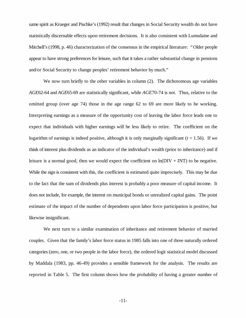
same spirit as Krueger and Pischke’s (1992) result that changes in Social Security wealth do not have

statistically discernable effects upon retirement decisions. It is also consistent with Lumsdaine and

Mitchell’s (1998, p. 46) characterization of the consensus in the empirical literature: “Older people

appear to have strong preferences for leisure, such that it takes a rather substantial change in pensions

and/or Social Security to change peoples’ retirement behavior by much.”

We now turn briefly to the other variables in column (2). The dichotomous age variables

AGE62-64 and AGE65-69 are statistically significant, while AGE70-74 is not. Thus, relative to the

omitted group (over age 74) those in the age range 62 to 69 are more likely to be working.

Interpreting earnings as a measure of the opportunity cost of leaving the labor force leads one to

expect that individuals with higher earnings will be less likely to retire. The coefficient on the

logarithm of earnings is indeed positive, although it is only marginally significant (t = 1.56). If we

think of interest plus dividends as an indicator of the individual’s wealth (prior to inheritance) and if

leisure is a normal good, then we would expect the coefficient on ln(DIV + INT) to be negative.

While the sign is consistent with this, the coefficient is estimated quite imprecisely. This may be due

to the fact that the sum of dividends plus interest is probably a poor measure of capital income. It

does not include, for example, the interest on municipal bonds or unrealized capital gains. The point

estimate of the impact of the number of dependents upon labor force participation is positive, but

likewise insignificant.

We next turn to a similar examination of inheritance and retirement behavior of married

couples. Given that the family’s labor force status in 1985 falls into one of three naturally ordered

categories (zero, one, or two people in the labor force), the ordered logit statistical model discussed

by Maddala (1983, pp. 46-49) provides a sensible framework for the analysis. The results are

reported in Table 5. The first column shows how the probability of having a greater number of

-12-

participants in the labor force in 1985 varies with inheritance, conditional on the number of people

in the labor force in 1982, and interactions with inheritance.

As was the case for single individuals in Table 4, the direct effect of (log) inheritance is

positive and statistically insignificant, but the net effect of the direct and interaction effects indicates

a negative impact on labor supply. Specifically, the interaction effects with the indicator variables for

one worker in 1982 and two workers in 1982 are negative and larger in absolute value than the

coefficient on inheritance alone. The joint test of the hypothesis that all the inheritance coefficients

are equal to zero (a chi-square test equal to 11.7 with three degrees of freedom) has a p-value of

0.009. Unlike the case of the singles, the effect of inheritance is significant.17

The next question is whether this finding continues to hold after the inclusion of other

variables that might affect labor force participation. As before, in column (2) we augment the set of

right-hand side variables with variables related to age, number of dependents, earned income, and18

the sum of dividends and interest. The point estimates on the interaction terms suggest that if either

spouse participated in the labor market in 1982, then receipt of an inheritance reduces the probability

of participating in 1985. While these three coefficients are not all precisely estimated, jointly they are

significant at the 0.007 level, a result similar to that in column (1). 19

As with single individuals, it is useful to assess the quantitative implications of the multivariate

results. Again, we use the coefficients to simulate the impact of a 10 percent increase in inheritance

by evaluating the right-hand side variables at their means, computing the probabilities of zero, one,

or two workers, and then re-computing with inheritance raised by 10 percent. The computation

indicates that the increase in inheritance raises the probability of having zero workers by 0.004 (or

0.8 percent) lowers the probability of having one worker by 0.003 (or 0.8 percent), and decreases the

probability of having two workers by 0.001 (or 1.5 percent). Thus, the multivariate analysis suggests

-13-

the same conclusion as Table 2— an inheritance received by a family reduces the probability that both

spouses will continue to work, and increases the probability that both will retire. An income effect

seems to be operative and is statistically significant, although its magnitude is small.

A possible source of misspecification in our results arises from the fact that we cannot

distinguish between anticipated and unanticipated inheritances. Of course, there is no direct way to

decompose an inheritance into its anticipated and unanticipated components. However, it is possible

that children of a decedent are more likely to anticipate their inheritances than other relations. Hence,

comparing the labor supply responses of children with other recipients might shed some light on this

issue. We therefore defined a dichotomous variable that equaled one if the donee was a child of the

decedent and zero otherwise. We then augmented the equations in the second columns of Tables 4

and 5 with this variable and its interaction with the log of inheritance.20

The interaction term was statistically insignificant in the sample of single returns, with a

t-statistic of -0.021. In the joint return data, on the other hand, the interaction term was negative

(-1.094) with a t-statistic of -1.65. Taken together, these results suggest that being the child of a21

decedent has no effect on the impact of inheritance on retirement, a finding that does not reconcile

easily with free intertemporal optimization. However, one must take this observation with a grain

of salt, since we have no evidence that the interaction variable adequately reflects the extent to which

the inheritance is anticipated.

Earnings Changes

So far, our focus has been the income effect on retirement rates. However, even donees22

who stay in the labor force might be induced by income effects to reduce their hours of work and

hence earn less, ceteris paribus. Accordingly, in this section we examine how inheritance affects

earnings, conditional on staying in the labor force. Before presenting the results, we stress that some

-14-

caution is required in their interpretation. Imagine that we observe earnings falling as the size of

inheritance increases. One possibility is that hours of work have fallen. Alternatively, hours could

have stayed the same, and the wage rate fallen. The decline in the wage rate might be due to the fact

that with higher wealth, individuals may choose jobs with more “desirable” characteristics that have

lower wage rates. (However, we are aware of no empirical evidence that this phenomenon exists.)

With these caveats in mind, we analyzed the percentage change in earnings for those families

in which the number of earners is the same in 1982 and 1985. In terms of the matrices in Table 1,

these are the individuals in the lower right-hand cell. In Table 2 they occupy the cells on the diagonal

for families with one earner each year and with two earners each year. To begin, for the relevant

sample of single individuals, we estimated a regression of the percentage change in real earnings (log

of earnings in 1985 minus the log of earnings in 1982) on the logarithm of inheritance. The results

are reported in column (1) of Table 6. The coefficient on inheritance is negative (-0.037), but not

estimated precisely. In column (2) we add our age variables, the log of dividend and interest income,

and the number of dependents. The coefficient and standard error on ln (INH) are little changed. In

columns (3) and (4) we repeat the exercise for earnings on joint returns. Here, again, we have

negative inheritance effects, but they are closer to significant at conventional levels. To assess the

quantitative implications of these estimates, note that an increase in inheritance of 10 percent (or, just

over $10,000 for both single and married individuals) would reduce earnings on a single return by

0.48 percent and on a joint return by 0.61 percent. For a single individual, this is roughly $18 in

1985, while for a married couple the 1985 earnings would fall by $69 (both measured in 1982

dollars). Given the qualifications mentioned above, one must necessarily be cautious in interpreting

these results, but if one takes them at face value, they suggest that there is at best only a modest

income effect on the hours worked by the elderly.

-15-

4. Conclusions

We have examined tax-return-generated data on the labor force behavior of retirement-aged

people before and after they received inheritances. Taken together, the results suggest that the

income effects associated with retirement decisions are weak. For single people, we found no

statistically discernible differences in retirement behavior between individuals who received large and

small inheritances. For couples, the impact of inheritances was sometimes significant in a statistical

sense, but always quite small quantitatively. Similarly, conditional on remaining in the labor force,

inheritance exerted only a small impact on earnings. On this basis, we would expect that only

substantial changes in Social Security benefits would affect retirement decisions very much, a finding

that is consistent with much of the previous literature.

-16-

1. One important complexity ignored by the simple model is that the retirement decisiondepends not only on the level of benefits, but the pattern of their accrual. See Gruber andWise (1998).

2. Holtz-Eakin, Joulfaian, and Rosen (1993) analyze the labor supply decisions of youngermembers of this sample using a similar method.

3. The $300,000 cutoff corresponds roughly to the threshold for filing an estate tax returnduring this period. The actual threshold was $225,000 in 1982, $275,000 in 1983, and$325,000 in 1984.

4. The ages in our sample range from 62 to 70 in 1985.

5. For 1982 the deduction was 5 percent of earned income.

6. Schedule W earnings also include income from partnerships (Schedule E). Partnershipincome may be more indicative of tax shelter activity than participation in the labor force, soreturns with partnerships were deleted. However, when partnership returns are included,none of the substantive results reported below change.

7. Here and throughout we identify nonparticipation in the labor force as “retirement.” AsQuinn (1998) and others have noted, many Americans retire in stages rather than a singlestep. Further, some elderly people may “retire” from the labor force in one year and returnthe next. Nevertheless, many individuals do follow the one-step pattern, and it is commonin the literature to assume that once an elderly person leaves the labor force, he or she staysout. See, for example, Lumsdaine (1992).

8. The cutoffs were chosen to provide an adequate number of observations in each range, andthe substantive results are not sensitive to minor changes in the inheritance ranges. Theranges reflect net receipts of inheritances by the beneficiaries. We have no information onstate inheritance taxes paid by donees, but this is irrelevant for our purposes. In general, onestate tax returns one receives a dollar for dollar credit for inheritance taxes paid to states.The median ratios of inheritance to 1982 Adjusted Gross Income in the low, middle, and highinheritance groups are 0.309, 3.16, and 10.6 respectively.

9. Neither the pairwise nor joint differences are statistically significant.

Endnotes

The authors are respectively, affiliated with Syracuse University and NBER, the U.S.*

Department of Treasury, and Princeton University and NBER. The authors are grateful to theNational Science Foundation, Princeton’s Center for Economic Policy Studies, and the Center forPolicy Research at Syracuse University for financial support. They also thank Stephen Wu andRebecca Porcello for research assistance, Esther Gray for preparing the manuscript; and RobinLumsdaine, Olivia Mitchell, and members of Princeton’s Public Finance Working Group for usefulsuggestions.

-17-

10. The median ratios of inheritance to 1982 Adjusted Gross Income in the low, middle, and highinheritance groups are 0.199, 2.34, and 7.31 respectively.

11. An interesting question is how the transition matrices in Tables 1 and 2 would compare withthose in a “control group” that received no inheritances. In this context, it is important tonote that the median inheritance in our “low” groups is only about $5,000. From the point ofview of labor force participation decisions over a four-year period, the “low inheritance”groups may effectively serve as “no inheritance” groups. This conjecture was confirmedwhen we examined analogous transition matrices computed using 1982 and 1985 data fromthe PSID for comparably aged individuals who reported no inheritances between those twoyears. On a cell-by-cell basis, one could not reject the hypothesis that the transition rates inthe PSID data were the same as the corresponding rates from Tables 1 and 2.

12. After receiving an inheritance, the labor force participation rates in the low, middle, and highinheritance groups for the single returns are 36.9, 25.1, and 27.0, respectively. For the jointreturns, after inheritance the corresponding proportions of two-earner couples are 14.9, 11.6,and 7.6; and the proportions with no earners are 46.2, 50.0, and 55.0. (In no cases are thedifferences statistically significant.)

13. The substantive results are unchanged when the level of inheritance is used.

14. We obtain similar results using a specification in which the size of the inheritance is enteredin levels, as opposed to logarithms. In this instance, the point estimate of the interactioncoefficient is estimated with modestly greater precision, but the overall significance of theinheritance variables is essentially unchanged.

15. As noted in Table 3, we represent age by a series of dichotomous variables. (The omittedcategory is individuals 74 years and older.) Alternative specifications in which age wasentered as a logarithm or as a quadratic led to substantially the same results.

16. A chi-squared test of the hypothesis that the coefficients on log of inheritance and itsinteraction with lagged labor force participation are jointly equal to zero is 3.49 with twodegrees of freedom, which is significant only at the 0.17 level.

17. Using a specification in which the size of the inheritance is entered in levels rather thanlogarithms, the point estimates of the coefficients have the same pattern. Also, the overallstatistical significance of the inheritance variables is just as strong— the p-value is 0.01.

18. Recall that we only have the age of one spouse (the donee), and we cannot identify thatspouse. Thus, if a relatively young donee is married to an elderly person, the family iscategorized as being relatively young. If the elderly spouse retires from the labor force, thedata would then suggest a misleading relation between age and labor force activity. On theother hand, to the extent that spouses are close in age, this problem may not be too severe.In any case, the age variables should be interpreted with caution.

19. The chi-squared test with three degrees of freedom is 12.23. When inheritance is entered inlevels rather than logs, the joint significance level of the three coefficients is 0.0006.

-18-

20. The proportions of donees who are children are 0.14 and 0.21 in the single return and jointreturn samples, respectively.

21. For both joint and single returns, the other coefficients were essentially unchanged.

22. As Lumsdaine and Mitchell (1998) note, most of the empirical literature has examinedretirement as a discrete outcome.

Table 1. Labor Force Transitions: Single Returnsa

1985

0 1

0 166 3 Inheritance < 25,000

1982 (0.0102) 0.0102

0.982 0.018 N = 360

1 Mean Inheritance = $6,736

61 130 (5,683)

0.319 0.681 Median Inheritance = $5,000

(0.0337) (0.0337) Mean Age = 71.3

(5.43)

1985

0 1

0 102 2 $25,000 < Inheritance < $150,000

1982 (0.0135) (0.0135)

0.981 0.019 N = 191

1 41 46 (36,568)

0.471 0.529 Median Inheritance = $58,815

(0.0535) (0.0535) Mean Age in 1985 = 70.5

Mean Inheritance = $69,519

(5.20)

1985

0 1

0 85 4 $150,000 < Inheritance

1982 (0.0220) (0.0220)

0.955 0.045 N = 152

1 26 37 (282,323)

0.413 0.587 Median Inheritance =$294,415

(0.0620) (0.0620) Mean Age in 1985 = 69.1

Mean Inheritance = $389,538

(5.37)

In each cell, the first figure is the number of observations in the cell; the second figure isa

the proportion of observations in the associated row that fall in the cell; and the figure inparentheses is the standard error of the proportion. Figures to the right of each matrix indicatethe relevant inheritance range, the number of observations, the mean and median inheritance,and age. Where shown, numbers in parentheses are standard deviations.Source: See text.

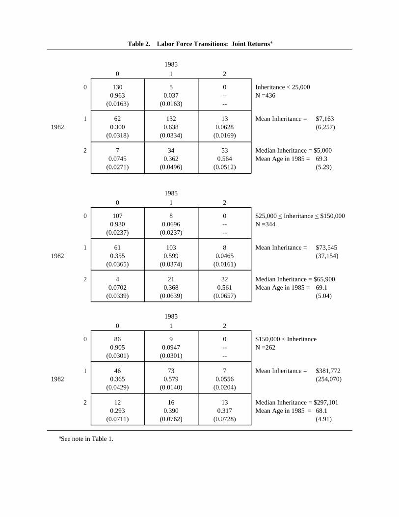
Table 2. Labor Force Transitions: Joint Returnsa

1985

0 1 2

0 130 5 0 Inheritance < 25,0000.963 0.037 -- N =436

(0.0163) (0.0163) --

1 62 132 13 Mean Inheritance = $7,1631982 0.300 0.638 0.0628 (6,257)

(0.0318) (0.0334) (0.0169)

2 7 34 53 Median Inheritance = $5,0000.0745 0.362 0.564 Mean Age in 1985 = 69.3

(0.0271) (0.0496) (0.0512) (5.29)

1985

0 1 2

0 107 8 0 $25,000 < Inheritance < $150,0000.930 0.0696 -- N =344

(0.0237) (0.0237) --

1 61 103 8 Mean Inheritance = $73,5451982 0.355 0.599 0.0465 (37,154)

(0.0365) (0.0374) (0.0161)

2 4 21 32 Median Inheritance = $65,9000.0702 0.368 0.561 Mean Age in 1985 = 69.1

(0.0339) (0.0639) (0.0657) (5.04)

1985

0 1 2

0 86 9 0 $150,000 < Inheritance0.905 0.0947 -- N =262

(0.0301) (0.0301) --

1 46 73 7 Mean Inheritance = $381,7721982 0.365 0.579 0.0556 (254,070)

(0.0429) (0.0140) (0.0204)

2 12 16 13 Median Inheritance = $297,1010.293 0.390 0.317 Mean Age in 1985 = 68.1

(0.0711) (0.0762) (0.0728) (4.91)

See note in Table 1.a

Table 3. Definitions of Variables and Summary Statisticsa

Variable Single Returns Joint Returns

ln(INH) 10.66 10.35

(log inheritance) (2.01) (1.98)

LF82 0.485 ---

(=1 if individual was in labor force in 1982) (0.501) ---

AGE62-64 0.180 0.241

(= 1 if 62 < age < 64 in 1985) (0.385) (0.428)

AGE65-69 0.250 0.348

(= 1 if 65 < age < 69 in 1985) (0.434) (0.477)

AGE70-74 0.282 0.227

(= 1 if 70 < age < 74 in 1985) (0.450) (0.419)

ln(EARN82) 4.24 6.07

(= log earnings in 1982) (4.56) (4.70)

ln(DIV + INT) 8.49 8.67

(= log dividends plus interest) (2.34) (2.28)

DEPENDENTS 0.0593 0.157

(= number of dependents claimed on return in 1982) (0.263) (0.567)

LF1’82 --- 0.485

(= 1 if one family member in labor force in 1982) --- (0.500)

LF2’82 --- 0.184

(=1 if two family members in labor force in 1982) --- (0.388)

N 703 1,042

Figures in parentheses are standard deviations.a

Table 4. Logit Analysis of Transition to Retirement: Single Returna

Variable (1) (2)

ln(INH) 0.1548 0.1027

(0.1774) (0.1800)

LF82 7.076 5.821

(2.027) (2.113)

ln(INH)*LF82 -0.2832 -0.2691

(0.1869) (0.1893)

AGE62-64 --- 0.7258

--- (0.3533)

AGE65-69 --- 1.014

--- (0.3364)

AGE70-74 --- -0.1047

--- (0.3378)

ln(EARN82) --- 0.09858

--- (0.06316)

ln(DIV + INT) --- -0.06009

--- (0.04865)

DEPENDENTS --- 0.1981

--- (0.4375)

Constant -5.290 -4.561

(1.936) (1.987)

Observations 703 703

loglikelihood -265.0 -253.0

Numbers in parentheses are standard errors, variables are defined in Table 3. Thea

dependent variable equals one if the individual was in the labor force in 1985 and zero

otherwise.

Table 5. Ordered Logit Analysis of Transition to Retirement: Joint Return a

Variable (1) (2)

ln(INH) 0.1964 0.1991

(0.1325) (0.1349)

LF1’82 5.822 4.625

(1.559) (1.608)

LF2’82 9.847 8.501

(1.669) (1.719)

LF1’82*ln(INH) -0.2346 -0.2365

(0.1397) (0.1416)

LF2’82*ln(INH) -0.4024 -0.4115

(0.1497) (0.1520)

AGE62-64 --- 0.2118

--- (0.2501)

AGE65-69 --- 0.09344

--- (0.2078)

AGE70-74 --- -0.1244

--- (0.2641)

ln(EARN82) --- 0.1255

--- (0.03366)

ln(DIV + INT) --- -0.04675

--- (0.03155)

DEPENDENTS --- 0.02920

--- (0.1230)

Constant -4.810 -4.412

(1.487) (1.511)

Observations 1,042 1,042

loglikelihood -694.1 -676.6

Numbers in parentheses are standard errors, variables are defined in Table 3. The dependenta

variable measures the probabilities of having zero, one, or two earners in the family in 1985.

R̄ 2

Table 6. Ordinary Least Squares Analysis of Earnings Changea

Variable (1) (2) (3) (4)

Single Returns Joint Returns

Constant -0.1164 -0.1241 0.0002493 -0.1869

(0.3566) (0.4050) (0.3306) (0.3847)

ln(INH) -0.03698 -0.04785 -0.05183 -0.06128

(0.03627) (0.03986) (0.03174) (0.03375)

AGE62-64 --- 0.3424 --- 0.2550

--- (0.2383) --- (0.2372)

AGE65-69 --- 0.04456 --- 0.08332

--- (0.2284) --- (0.2279)

AGE70-74 --- 0.0648 --- 0.2898

--- (0.2491) --- (0.2617)

ln(DIV + INT) --- -0.003409 --- 0.01044

--- (0.02692) --- (0.02482)

DEPENDENTS --- 0.09164 --- 0.1254

--- (0.2473) --- (0.08467)

0.00021 -0.00215 0.00526 0.00695

Observations 186 186 314 314

Numbers in parentheses are standard errors. The dependent variable is the percentage change in earningsa

between 1982 and 1985, conditional on the number of earners in the family being the same in both years.

Variables are defined in Table 3.

-25-

References

Barro, Robert, 1974. “Are Government Bonds Net Wealth?” Journal of Political Economy,LXXXII: 1095-1117.

Costa, Dora L. 1995. “Pensions and Retirement: Evidence from Union Army Veterans,” QuarterlyJournal of Economics (May): 297-319.

Friedberg, Leora. 1998. “The Effect of Old Age Assistance on Retirement.” NBER Working PaperNo. 6548. Cambridge: National Bureau of Economic Research, May.

Gruber, Jonathan and David Wise. 1998. “Social Security and Retirement: An InternationalComparison,” American Economic Review (May): 158-163.

Holtz-Eakin, Douglas, David Joulfaian, and Harvey S. Rosen. 1993. “The Carnegie Conjecture:Some Empirical Evidence,” Quarterly Journal of Economics (May): 413-435.

Krueger, Alan B. and Jorn-Steffen Pischke. 1992. “The Effect of Social Security on Labor Supply:A Cohort Analysis of the Notch Generation,” Journal of Labor Economics (October): 412-437.

Lumsdaine, Robin L. 1992. “Three Models of Retirement: Computational Complexity versusPredictive Validity.” In David Wise (ed.), Topics in the Economics of Aging. Chicago:University of Chicago Press, pp. 19-57.

Lumsdaine, Robin L. and Olivia S. Mitchell. 1998. “New Developments in the Economic Analysisof Retirement,” Pension Research Council Working Paper No. 98-8. Philadelphia: Universityof Pennsylvania, February.

Maddala, G.S. 1983. Limited Dependent and Qualitative Variables in Econometrics. Cambridge,MA: Cambridge University Press.

Neumark, David and Elizabeth Powers. 1998. “Welfare for the Elderly: The Effects of SSI on Pre-Retirement Labor Supply,” NBER Working Paper No. 6805. Cambridge, MA: NationalBureau of Economic Research, November.

Pope, Clayne L. and Larry T. Wimmer. 1998. “Aging in the Early 20 Century,” Americanth

Economic Review (May): 217-221.

Quinn, Joseph. 1998. “New Paths to Retirement,” Pension Research Council Working Paper No.98-10. Philadelphia: University of Pennsylvania, October.

Rust, John and Christopher Phelan. 1997. “How Social Security and Medicare Affect RetirementBehavior in a World of Incomplete Markets, Econometrica, 65: 781-832.

AGING STUDIES PROGRAM PAPERS

PaperNo. Title Author Date

1 The Division of Family Labor: Care for Wolf, Freedman, and August 1995Elderly Parents Soldo

2 Time? Money? Both? The Allocation of Couch, Daly, and December 1995Resources to Older Parents Wolf

3 Coresidence with an Older Mother: The Soldo, Wolf, and December 1995Adult Child’s Perspective Freedman

4 Determinants and Consequences of Schneider and Wolf January 1997Multigenerational Living Arrangements:The Case of Parent-Adult ChildCoresidence

5 Do Parents Divide Resources Equally Dunn and Phillips January 1997among Children? Evidence from theAHEAD Survey

6 Late Life Job Displacement Couch January 1997

7 The Immigrant Sample of the German Burkhauser, January 1997Socio-Economic Panel Kreyenfeld, and

Wagner

8 Testing the Significance of Income Burkhauser, Crews, June 1997Distribution Changes Over the 1980s Daly, and JenkinsBusiness Cycle: A Cross-NationalComparison

9 Changes in Economic Well-Being and Burkhauser and Crews June 1997Income Distribution in the 1980s:Different Measures, Different Outcomes

10 How Older People in the United States Crews and Burkhauser August 1997and Germany Fared in the Growth Yearsof the 1980s— A Cross-Sectional versus aLongitudinal View

11 Health, Work, and Economic Well-Being Burkhauser, Dwyer, August 1997of Older Workers, Aged 51 to 61: A Lindeboom,Cross-National Comparison Using the Theeuwes, andUnited States HRS and The Netherlands WoittiezCERRA Data Sets

AGING STUDIES PROGRAM PAPERS

PaperNo. Title Author Date

12 Estimating Federal Income Tax Burdens Butrica and December 1997for Panel Study of Income Dynamics Burkhauser(PSID) Families Using the NationalBureau of Economic Research TAXSIMModel

13 Elderly Migration and State Fiscal Policy: Conway and August 1998Evidence from the 1990 Census Migration HoutenvilleFlows

14 Intergenerational Co-Residence and Dunn and Phillips October 1998Children’s Incomes

15 When Random Group Effects are Cross- Conway and October 1998Correlated: An Application to Elderly HoutenvilleMigration Flow Models

16 Residential Choices and Prospective Risks Couch and Kao November 1998of Nursing Home Entry

17 Traditionality, Modernity, and Household Aykan and Wolf November 1998Composition: Parent-Child Coresidencein Contemporary Turkey.

18 Estimating the Income Effect on Holtz-Eakin, Joufaian, April 1999Retirement and Rosen