Working Paper 339August 2013

Estimating Income/Expenditure Differences across Populations: New Fun with Old Engel’s Law

Abstract

How much larger are the consumption possibilities of an urban US household with per capita expenditures of 1,000 US dollars per month than a rural Indonesian household with per capita expenditures of 1,000,000 Indonesian Rupiah per month? Consumers in different markets face widely different consumption possibilities and prices and hence the conversion of incomes or expenditures to truly comparable units of purchasing power is extremely difficult. We propose a simple supplement to existing purchasing power adjusted currency conversions.

The Pritchett-Spivack Ratio (PSR) estimates the differences in household per capita expenditure using a simple inversion of the Engel’s law relationship between the share of food in consumption and total income/expenditures. Intuitively, we ask: “How much higher (as a ratio) would the expenditures of a household at 1,000,000 Indonesian Rupiah need to be along a given Engel relationship before they were predicted to have the same food share as a US household with consumption of 1,000 US dollars?” The striking empirical stability of Working-Lesser Engel coefficient estimates across time and space and widely available estimates of consumptions expenditures and hence food shares allow us to make two robust points using the PSR.

First, the consumption of the typical (median) household in a developing country would have to rise 5 to 10 fold to reach that of a household at the poverty line in an OECD country. Second, even the “rich of the poor”—the 90th or 95th percentile in developing countries—have food shares substantially higher than the “poor of the rich.”

JEL Codes: O10, I32, D12, D31

Keywords: Engel curve, material standard of living, international development, poverty assessment income inequality.

www.cgdev.org

Lant Pritchett and Marla Spivack

Estimating Income/Expenditure Differences across Populations: New Fun with Old Engel’s Law

Lant PritchettHarvard Kennedy School

Senior Fellow, Center for Global Development

Marla SpivackCenter for Global Development

We are grateful to Charles Kenny and two anonymous reviewers for useful comments. All errors and opinions are our own.

CGD is grateful for support of this work from its board of directors and funders, including the William and Flora Hewlett Foundation, the Norwegian Ministry of Foreign Affairs, the UK Department for International Development, and the Swedish Ministry of Foreign Affairs.

Lant Pritchett and Marla Spivack . 2013. "Estimating Income/Expenditure Differences across Populations: New Fun with Old Engel’s Law." CGD Working Paper 339. Washington, DC: Center for Global Development.http://www.cgdev.org/publication/estimating-incomeexpenditure-differences-across-populations-new-fun-old-engel’s-law

Center for Global Development1800 Massachusetts Ave., NW

Washington, DC 20036

202.416.4000(f ) 202.416.4050

www.cgdev.org

The Center for Global Development is an independent, nonprofit policy research organization dedicated to reducing global poverty and inequality and to making globalization work for the poor. Use and dissemination of this Working Paper is encouraged; however, reproduced copies may not be used for commercial purposes. Further usage is permitted under the terms of the Creative Commons License.

The views expressed in CGD Working Papers are those of the authors and should not be attributed to the board of directors or funders of the Center for Global Development.

Contents

1. Introduction ............................................................................................................................. 1

2. The Pritchett-Spivack Ratio ................................................................................................... 4

2.1 Why a new comparison of material standard of living? .................................................. 4

2.2 The calculation ....................................................................................................................... 5

2.3 Benefits of the PSR ............................................................................................................... 8

3. Estimating the simple Engel coefficient .............................................................................. 8

4. “Ground-truthing” the PSR with historical episodes ....................................................... 11

5. Applications ........................................................................................................................... 13

5.1 How much growth is needed? ........................................................................................... 13

5.2 Are the “rich” in poor countries rich? ............................................................................. 21

6. Conclusion .............................................................................................................................. 26

References ....................................................................................................................................... 27

Appendix ......................................................................................................................................... 29

1

1. Introduction

Many discussions about post-2015 development goals are dominated by concerns about (a)

“sustainability”1 (b) the plight of the “poor of the poor” (if not the “poorest of the poor”)

based on the penurious “dollar a day” standard or its ilk, (c) the minimalist standards on

well-being indicators (Kenny and Pritchett 2013) embodied in the current Millennium

Development Goals and (d) “inequality” in outcomes across groups within countries. The

“post-materialist” concerns which empirically predominate in the richest countries (Inglehart

1997)) are very much in evidence. One might even get the impression that, while material

standard of living standard of the “bottom billion” was a global concern, everyone else was

doing fine2. In fact, given the frequency with which the words “consumption” and

“sustainable” are paired one might think the most pressing concern with the current

consumption “middle of the middle”—the median household in the world--was that it was

too high or growing too quickly.

This lack of urgency for improving the material standard of living of the five billion people

in the middle (neither in dollar a day poverty nor in the top billion) is not because the

incomes in poor countries have “converged.” Comparing GDP per capita in 2010 of the

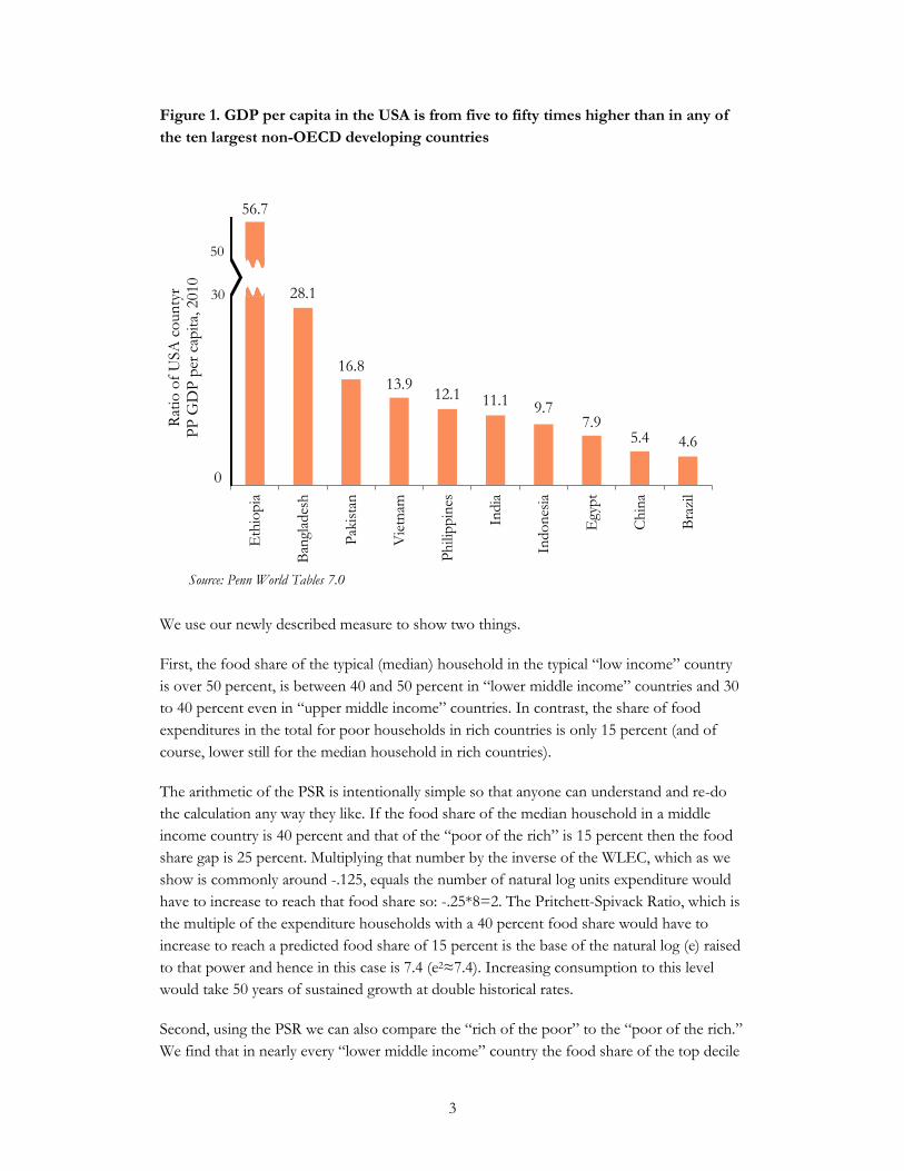
USA to the ten largest non-OECD developing countries3 shows ratios from 50 times to 1 in

Ethiopia to around 10 to 1 in “low middle income” countries like India and Indonesia to 5

to 1 in “upper middle income” countries like China and Brazil. But comparisons of GDP are

increasingly out of favor. From Robert Kennedy4 to the Sarkozy-Stiglitz Commission there

have been criticisms of GNP as a relevant measure for human well-being. At high levels of

material well-being it is natural that post-material concerns like “the beauty of our poetry”

(part of RFK’s critique of GNP) become important. This is sharpened, of course, by the

inadequate accounting for natural resources and their depletion in the measured GNP.

Moreover, per capita GDP (or consumption) says nothing about the distribution of

consumption possibilities among the individuals within the economy.

1 The General Secretary of the UN has explicitly stated that the “development” and “sustainability” objectives

should be merged in the post-2015 framework.

2 Of course Paul Collier’s “bottom billion” (2007) put attention on Africa and “fragile” and conflict states by

ignoring the equally poor half billion of South Asia (Ghani 2010) and the poor of other regions on the premise

that, although equally poor, these people resided in countries that were, on average, growing.

3 Mexico’s joining of the OECD makes the usual shorthand of “developed” and “OECD” problematic. Here we

exclude Mexico, and when we want to refer to the developed countries, we use the phrase “rich OECD” which

excludes the more recent joiners.

4 He famously said of GDP that “it measures everything in short, except that which makes life worthwhile.”

2

However, even eschewing GNP and examining global inequalities using household survey

based incomes or expenditures across countries (e.g. Milanovic 2013b) leaves the challenge

of comparisons of the purchasing power households. Two households in Cleveland, one

making $50,000 a year and one making $20,000 a year can buy in the same grocery stores,

rent from the same housing stock, could get haircuts from the same salons and get electricity

from the same utility. Since they the same possibilities and prices money incomes proxy well

for consumption possibilities. But how does one compare “true” purchasing power between

a household spending $20,000 in Cleveland versus 1,000,000 Rupiah in Semerang Indonesia

versus 50,000 Rupees in Chennai India? While the International Comparisons Project and its

successors and partners have made enormous strides in the quality of estimates of PPP

currency conversions, the sheer conceptual and empirical complexity of the exercise—

especially quality adjusted price comparisons of non-traded goods and services--can leave

both the “man on the street” and the expert skeptical5.

In this paper we present a new measure, the Pritchett-Spivack Ratio, for comparing

consumption possibilities across countries (or groups within countries) using average food

shares. Our measure is free of all three of the previous objections. First, we use no national

accounts data at all. None of the criticisms of GDP apply. Second, our measure is always

based on specifics of the distribution of consumption across households. Third, we require

no international measures of prices. Nothing of course is a free lunch. Our measure buys

simplicity and intuitive appeal at the cost of dependence on the stability of Engel’s Law.

The Pritchett-Spivack Ratio is the ratio of the expenditures it would take for the observed

food share of any one group (say, the median urban household in Indonesia or the 95th

percentile household in rural Ethiopia) to reach, by moving along an Engel relationship

between food share and total consumption, the food share of another group (say, the

bottom 20th percentile in the USA or the median in Denmark). The PSR simply uses the

Engel curve to translate differences in food shares (vertical axis) into differences in

expenditures (horizontal axis). With the Working-Leser (Working, 1943; Leser, 1963)

specification of the Engel relationship, which relates the food share of expenditure linearly

to the natural log of total household expenditures, the PSR takes a very simple and intuitive

formula which depends on the Working-Leser Engel Coefficient.

5 For instance, Deaton, Friedman, and Alatas (2004) use household data on prices to estimate PPP conversions

for India versus Indonesia and find very different results than the standard comparisons.

3

Figure 1. GDP per capita in the USA is from five to fifty times higher than in any of

the ten largest non-OECD developing countries

We use our newly described measure to show two things.

First, the food share of the typical (median) household in the typical “low income” country

is over 50 percent, is between 40 and 50 percent in “lower middle income” countries and 30

to 40 percent even in “upper middle income” countries. In contrast, the share of food

expenditures in the total for poor households in rich countries is only 15 percent (and of

course, lower still for the median household in rich countries).

The arithmetic of the PSR is intentionally simple so that anyone can understand and re-do

the calculation any way they like. If the food share of the median household in a middle

income country is 40 percent and that of the “poor of the rich” is 15 percent then the food

share gap is 25 percent. Multiplying that number by the inverse of the WLEC, which as we

show is commonly around -.125, equals the number of natural log units expenditure would

have to increase to reach that food share so: -.25*8=2. The Pritchett-Spivack Ratio, which is

the multiple of the expenditure households with a 40 percent food share would have to

increase to reach a predicted food share of 15 percent is the base of the natural log (e) raised

to that power and hence in this case is 7.4 (e2≈7.4). Increasing consumption to this level

would take 50 years of sustained growth at double historical rates.

Second, using the PSR we can also compare the “rich of the poor” to the “poor of the rich.”

We find that in nearly every “lower middle income” country the food share of the top decile

28.1

16.8 13.9

12.1 11.1 9.7 7.9

5.4 4.6

56.7

Eth

iop

ia

Ban

glad

esh

Pak

ista

n

Vie

tnam

Ph

ilip

pin

es

India

Indo

nes

ia

Egy

pt

Ch

ina

Bra

zil

50

30

Source: Penn World Tables 7.0

Rat

io o

f U

SA

co

un

tyr

P

P G

DP

per

cap

ita,

2010

0

4

is roughly twice as high (around 25 to 30 percent) as the food share of the poor in rich

OECD. This implies that the even the “rich of the middle income” would have to have

expenditures at least twice as high (e.g. exp((.25-.15) /.125)=2.2) to reach the same food share

as the poor in rich countries. Even in upper middle income countries like Peru the food share

of “the rich” barely reaches that of the OECD poor.

These calculations are not an alternative to existing comparisons of either national accounts

consumption data or household income/expenditure using PPP exchange rates, but rather a

supplement. They confirm the findings of previous studies which have compared welfare

across groups using PPP expenditure and income estimates (Birdsall 2010). Our calculations

add some simple “common sense” credibility based only on easily available data about actual

consumption choices of households to the much, much, more complex and sophisticated

calculations of GDP and of PPP exchange rates. Both come to the conclusion that the core

global agenda for development, if it is to be all relevant to most people on the planet, has to

continue to focus squarely on expanding the productivity of people around the world to

endow them with choices that are both adequate to human well-being and globally fair.

2. The Pritchett-Spivack Ratio

2.1 Why a new comparison of material standard of living?

There are two dominant ways of comparing material standards of living across countries:

national accounts and survey estimates. The national accounts estimates of GDP per capita

or consumption per capita suffer from (at least) four difficulties. First, there is the intrinsic

difficulty of making comparable estimates of national accounts across countries. Second, the

“consumption” component of GDP is often the least well measured (and in fact is often

measured as a residual). Third, the national accounts estimates produce a single number of

aggregate consumption and provide no information about the distribution of consumption

across households. Fourth, national accounts are produced in local currency and hence an

exchange rate is needed.

Comparisons using measures of income or expenditure directly from household surveys

solve three of these four difficulties, while adding a new concern. The new concern is

whether the concept of “expenditure” is measured similarly across countries. Household

survey estimates of income or consumption are also in local currency and hence cross-

national comparisons require a conversion factor from one currency to another.

The well-known problem is that non-tradable goods and services (like getting a haircut) are

cheaper in poor countries and hence using market determined exchange rates – even if these

exchanges rates were to establish PPP in tradable goods – will overstate the differences in

purchasing power between a rich and poor country, because they do not account for cheaper

non-tradables. The International Comparisons Project (ICP) and its successors have made

heroic efforts since the 1970s to collect and process the data needed to create Purchasing

Power equivalent exchange rates, the exchange rate such that a rupee converted into a

5

common currency, say dollars, at that exchange rate represents equal command over

resources in India as in the USA. These PPP exchange rates are now routinely used by all

international comparisons of either national accounts (as for instance in the Penn World

Tables or the World Bank’s estimates) and are used for comparisons of household surveys

(e.g. Milanovich 2013b).

Almas (2007) used household micro-data to calculate Engel curves across nine different

countries and, relying on the observed stability of the Engel curves, imposes a common

Engel relationship across the countries to estimate the bias in the Penn World Tables PPP

calculations. He finds that PPP exchanges rates overestimate income of poor countries, with

the a greater bias the poorer the country. Hence international inequality in living standards is

systemically underestimated by the conventional estimates of GDP or consumption per

capita.

We build on this previous work, exploiting micro and grouped data to estimate Engel

elasticities for many more countries. However our method relies only on the stability of the

Engel curve within countries and we never explicitly calculate income differences or prices

across countries. We are proposing an additional alternative to estimating PPP rather than an

alternative estimate of PPP or a substitute for PPP. Our comparisons and PPP have different

strengths and weaknesses and, while we will compare our estimates to PPP there is no

default assumption that PPP comparisons are the “gold standard” which we are trying to

achieve nor, conversely, do we attempt to make generalizations about the validity of PPP.

2.2 The calculation

Since proposed by Ernst Engel in 1857 the conjecture that more prosperous households

spend a lower fraction of their expenditures (or income) on food (or, alternatively, that the

income/consumption elasticity of food expenditure is less than one) has become the most

widely replicated empirical relationship in all of the social sciences. Moreover, an extremely

simple specification of Engel’s Law—that the household share of expenditures on food is

linearly related to the natural log of total consumption expenditures (or income) known as

the Working-Leser form—has been shown to be robust and reliable functional form.

Whether data across households within a country/region, across income or consumption

groups within a country/region, across time in a country/region, or across countries/regions

is used the estimated WLEC is consistently centered between -.1 and -.15.

Our new fun with the old Engel Law is to simply “invert” it. Usually one thinks of the

Engel curve as “predicting” the food share for a given level of expenditures but we use the

same linear relationship to “estimate” the difference in expenditures implied by differences

in food shares. As simplicity and straightforward intuition are two desirable features we

want to stress how stubbornly simple our calculation is (while acknowledging the sacrifices

for this simplicity) using Figure 2. In a standard Engel graph with food share on the vertical

axis and natural log ependitures on the horizontal the difference in food shares between the

actual of some group (e.g. the median in Rural India or 95th percent of Peru) and a “target”

6

food share is just the vertical “rise.” We want to know the “run”—the difference in (ln)

expenditures that along a given Engel relationship would produce a “predicted” at that level

of expenditures equal to the target. In the linear case this not calculus, or even algebra, it is

just simple arithmetic: the “run” is just equal to the “rise” (difference in food shares) times

the “run over the rise” which is just the inverse of the linear slope. This gives the difference

in natural log units. Then by the properties of natural logs (that the difference in natural logs

is the log of the ratio) the ratio of the levels of expenditures is just e (≈2.714, the base of the

natural log) raised to that power.

Figure 2. Graphic illustration of the calculation of the Pritchett-Spivack ratio

The PSR formulation is general and can be calculated using any functional form of the Engel

relationship, but in the PSR-WL specification it takes the very simple form (assuming in this

case target is lower than actual so the numerator and denominator are both negative):

( )

(

)

Whether expenditures are measured in rupiah, rupee, lira, or pesos doesn’t matter as the PSR

never transforms the units of expenditure. The counter-factual is “as a household expanded

its consumption along a simple linear Engel relationship how much higher would

consumption have to be in those units and at the same consumption possibilities before the predicted

household food share reached the target?”

Ln(consumption)

Estimated Working-Leser Engel Curve (WLEC=ε) Food

share of median household

Ln(cmedian

)

Target food share

Ln(ctarget foodshare)

Fo

od S

har

e

Source: authors.

7

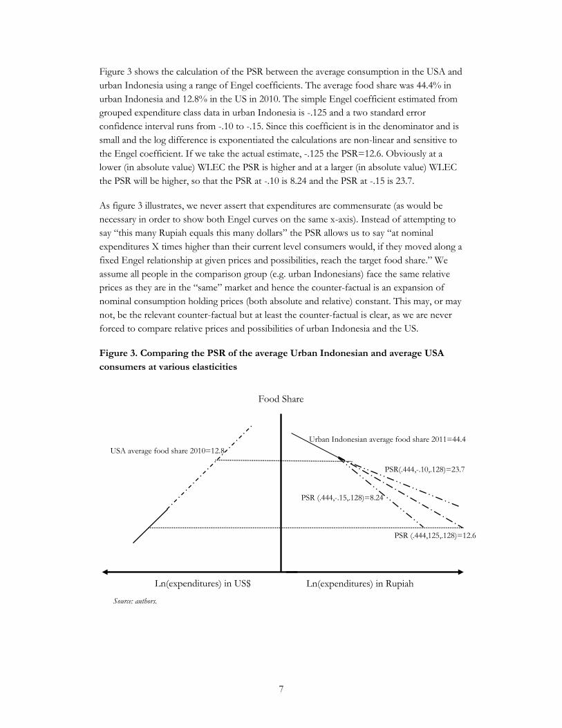
Figure 3 shows the calculation of the PSR between the average consumption in the USA and

urban Indonesia using a range of Engel coefficients. The average food share was 44.4% in

urban Indonesia and 12.8% in the US in 2010. The simple Engel coefficient estimated from

grouped expenditure class data in urban Indonesia is -.125 and a two standard error

confidence interval runs from -.10 to -.15. Since this coefficient is in the denominator and is

small and the log difference is exponentiated the calculations are non-linear and sensitive to

the Engel coefficient. If we take the actual estimate, -.125 the PSR=12.6. Obviously at a

lower (in absolute value) WLEC the PSR is higher and at a larger (in absolute value) WLEC

the PSR will be higher, so that the PSR at -.10 is 8.24 and the PSR at -.15 is 23.7.

As figure 3 illustrates, we never assert that expenditures are commensurate (as would be

necessary in order to show both Engel curves on the same x-axis). Instead of attempting to

say “this many Rupiah equals this many dollars” the PSR allows us to say “at nominal

expenditures X times higher than their current level consumers would, if they moved along a

fixed Engel relationship at given prices and possibilities, reach the target food share.” We

assume all people in the comparison group (e.g. urban Indonesians) face the same relative

prices as they are in the “same” market and hence the counter-factual is an expansion of

nominal consumption holding prices (both absolute and relative) constant. This may, or may

not, be the relevant counter-factual but at least the counter-factual is clear, as we are never

forced to compare relative prices and possibilities of urban Indonesia and the US.

Figure 3. Comparing the PSR of the average Urban Indonesian and average USA

consumers at various elasticities

Food Share

Ln(expenditures) in US$ Ln(expenditures) in Rupiah

Urban Indonesian average food share 2011=44.4

USA average food share 2010=12.8

PSR (.444,125,.128)=12.6

PSR (.444,-.15,.128)=8.24

PSR(.444,-.10,.128)=23.7

Source: authors.

8

2.3 Benefits of the PSR

The principal attractions of the PSR are four-fold. First, it makes intuitive sense to the

“woman on the street”—if rich people spend less on food then we can compare who is rich

and who is poor (and by how much) by comparing how much they spend on food. This

does not depend on understanding or believing either national accounts or PPP

comparisons. Second, the data on food shares from household surveys is widely available

across countries. Since the weights in a consumer price index depend on consumption

shares, nearly every country in the world has done an expenditure survey and many countries

do them at frequent intervals. Third, since nearly all expenditure surveys are divided into

income or expenditure classes the food share comparisons can be made at various points of

the country income distribution. Fourth, the PSR is “plug and play” as we are not insisting

that the PSR be used with any particular Engel coefficient—or even that one use a simple

functional form of the Engel relationship. Just plug in any values of the three inputs, actual

food share (of any percentile of the consumption distribution), a target food share (chosen in

any way desired), and any functional form of the predicted Engel relationship and viola one

has a PSR.

There are many, many limitations to the PSR and we are not overselling its value. First, we

want to be clear we are not proposing that the food share is a well-defined measure of

human well-being. However, the food share is a useful proxy for household consumption

possibilities at an aggregate level. If we compare the food share at the 20th percentile of

income in Colombia to the food share at the 20th percentile of income in Indonesia we have

tens of thousands of households of different shapes and sizes smoothed together and

aggregated, and we can reasonably compare the welfare of the aggregated 20th percentile

households in Colombia and Indonesia.

The Engel curve is an empirically reliable tendency, which gives the food share a rough and

ready usefulness, but the food share is not measure of human well-being that could be

axiomatically derived and defended. In particular, we are not proposing the food share for

comparisons across households within a population, as the differences in food needs of

households of different sizes, demographic structures, etc. make the food share vary for

reasons having nothing to do with ranking households’ “true” income. We are proposing the

PSR as a new simple calculation that, by taking advantage of the consistency of the elasticity

of the Engel curve, allows us to make easy to understand and compute comparisons between

groups, and draw useful conclusions about the differences in welfare between groups.

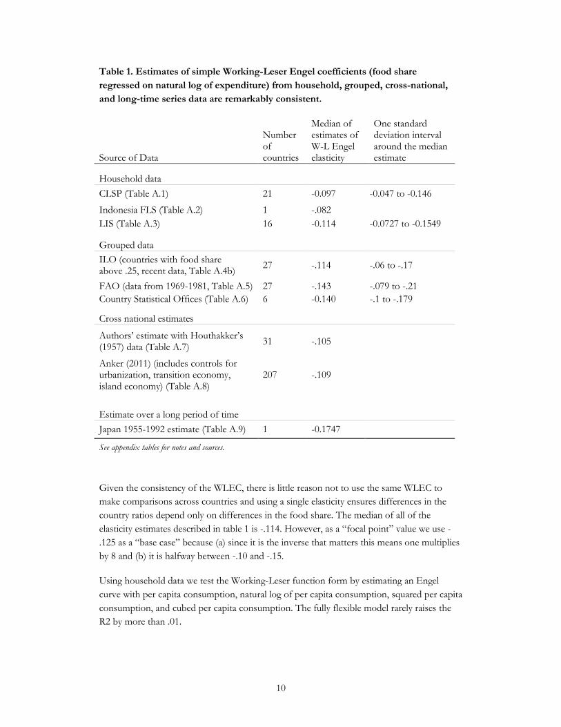
3. Estimating the simple Engel coefficient

The simplest form of the PSR-WL hinges on an Engel relationship in which the food share

is linearly related to the natural log of expenditure and for which the slope (WLEC) can be

known with some precision. Fortunately, the W-L Engel curve is one of the most widely

estimated and one of the most remarkably stable empirical relationships in all of economics

(indeed in all of the social sciences). This paper is not a contribution to the voluminous

literature estimating Engel curves, with literally thousands of papers. We use three different

9

types of data sources to estimate Engel curves, household micro data, grouped data that has

been compiled by international organizations, and group data accessed from country

statistical office reports. We show elasticity estimates in this paper simply to show that the

most straightforward ways of estimating the simple Engel coefficient, all, in spite of their

several defects, produce estimates that cluster in the range of -.10 to -.15.

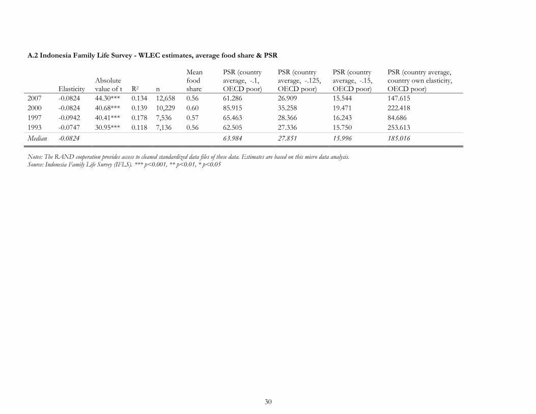
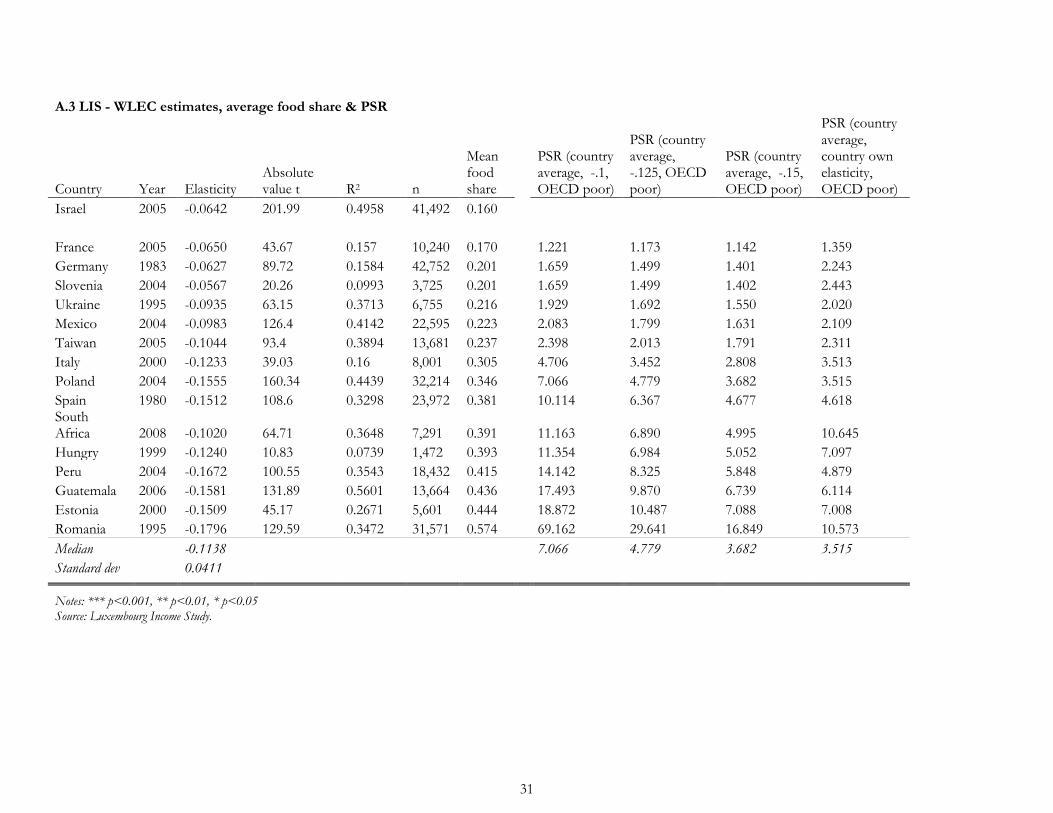
Estimates from household data micro data. We use household micro data from three sources: the

Comparative Living Statistics Project, the Luxembourg Income Study, and the Indonesia

Family Life Survey. These sources allow us to compute the WLEC using household data for

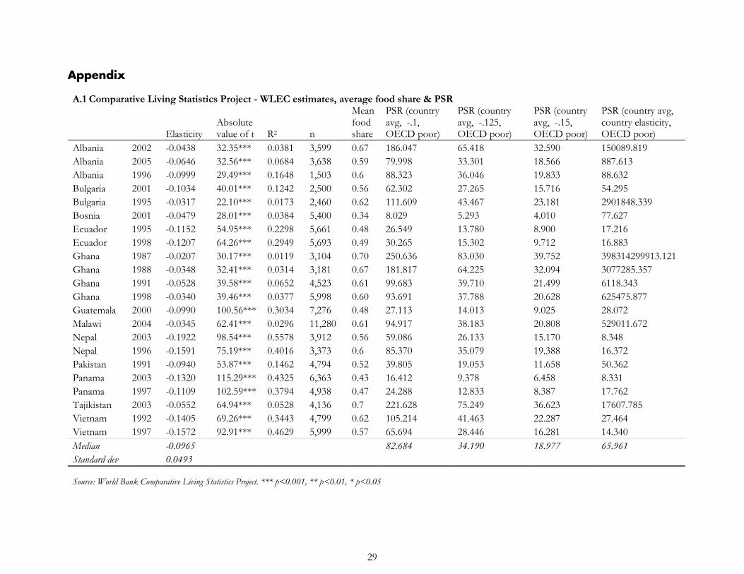
38 countries from various years. Table 1 (summarizing results reported in Appendix Tables

A1, A2 and A3) show these household based estimates cluster around -.1.

Estimates from grouped/percentile data. The WLEC can be estimated using grouped data on food

share and consumption expenditures, such as deciles, quintiles, or consumption/income

brackets. The International Labor Organization (ILO) maintains a database of estimates of

consumer expenditures used in estimating consumer price indices, and we use those data to

estimate the WLEC for these countries. Similarly, a 1981 FAO publication includes grouped

data for 27 countries for years ranging from 1969-1979. Country statistical offices also

publish this data in statistical abstracts and online databases, which we gather for key

countries.

Estimates across countries. At the 100 year anniversary Houthakker computed Engel elasticities

for 31 countries for various years between 1853 and 1955, with multiple survey years for

some. He found an elasticity slightly different from Engel’s 1857 finding, but consistent in

direction and magnitude. Houthakker did not use the WLEC functional form, but here we

use the summary statistics reported in his paper to estimate the WLEC across the countries

in his study. The cross national elasticity from this historical data is -.105 Later at the 150th

anniversary of Engel’s publication introducing the empirical law between income and

consumption, Anker (2011) constructs a data set of food shares for 207 countries and uses

this to estimate the WLEC across countries. His point estimate is -.109, a number which he

shows is quite robust whether one allows for non-linearity or disaggregates the countries by

income level. nearly

Estimates from over long periods. The WLEC can also be estimated over long periods of time,

with historical data on household expenditures by categories. Japan publishes harmonized

data on household expenditures by income groups for almost every year between 1926 and

2007, which we use to estimate the WLEC for the 38 years between 1955 and 1992.6 The

WLEC estimate across this seven decade period is -.175.

6 We begin the analysis in 1955 because that is the first year for which CPI data are available. We end in 1992 to

leave out the years during and after Japan’s economic crisis.

10

Table 1. Estimates of simple Working-Leser Engel coefficients (food share

regressed on natural log of expenditure) from household, grouped, cross-national,

and long-time series data are remarkably consistent.

Source of Data

Number of countries

Median of estimates of W-L Engel elasticity

One standard deviation interval around the median estimate

Household data

CLSP (Table A.1) 21 -0.097 -0.047 to -0.146

Indonesia FLS (Table A.2) 1 -.082

LIS (Table A.3) 16 -0.114 -0.0727 to -0.1549

Grouped data

ILO (countries with food share above .25, recent data, Table A.4b)

27 -.114 -.06 to -.17

FAO (data from 1969-1981, Table A.5) 27 -.143 -.079 to -.21

Country Statistical Offices (Table A.6) 6 -0.140 -.1 to -.179

Cross national estimates

Authors’ estimate with Houthakker’s (1957) data (Table A.7)

31 -.105

Anker (2011) (includes controls for urbanization, transition economy, island economy) (Table A.8)

207 -.109

Estimate over a long period of time

Japan 1955-1992 estimate (Table A.9) 1 -0.1747

See appendix tables for notes and sources.

Given the consistency of the WLEC, there is little reason not to use the same WLEC to

make comparisons across countries and using a single elasticity ensures differences in the

country ratios depend only on differences in the food share. The median of all of the

elasticity estimates described in table 1 is -.114. However, as a “focal point” value we use -

.125 as a “base case” because (a) since it is the inverse that matters this means one multiplies

by 8 and (b) it is halfway between -.10 and -.15.

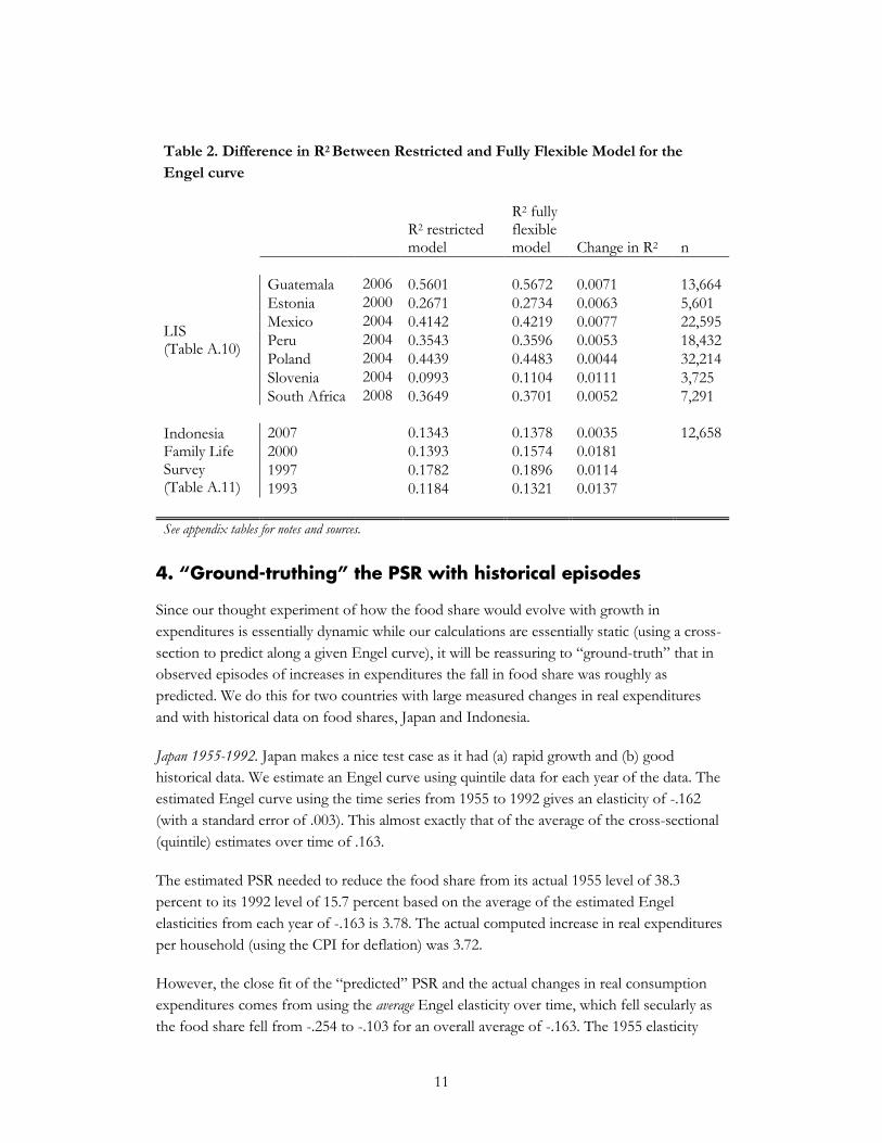
Using household data we test the Working-Leser function form by estimating an Engel

curve with per capita consumption, natural log of per capita consumption, squared per capita

consumption, and cubed per capita consumption. The fully flexible model rarely raises the

R2 by more than .01.

11

Table 2. Difference in R2 Between Restricted and Fully Flexible Model for the

Engel curve

R2 restricted model

R2 fully flexible model Change in R2 n

LIS (Table A.10)

Guatemala 2006 0.5601 0.5672 0.0071 13,664

Estonia 2000 0.2671 0.2734 0.0063 5,601

Mexico 2004 0.4142 0.4219 0.0077 22,595

Peru 2004 0.3543 0.3596 0.0053 18,432

Poland 2004 0.4439 0.4483 0.0044 32,214

Slovenia 2004 0.0993 0.1104 0.0111 3,725

South Africa 2008 0.3649 0.3701 0.0052 7,291

Indonesia Family Life Survey (Table A.11)

2007 0.1343 0.1378 0.0035 12,658

2000 0.1393 0.1574 0.0181 1997 0.1782 0.1896 0.0114 1993 0.1184 0.1321 0.0137

See appendix tables for notes and sources.

4. “Ground-truthing” the PSR with historical episodes

Since our thought experiment of how the food share would evolve with growth in

expenditures is essentially dynamic while our calculations are essentially static (using a cross-

section to predict along a given Engel curve), it will be reassuring to “ground-truth” that in

observed episodes of increases in expenditures the fall in food share was roughly as

predicted. We do this for two countries with large measured changes in real expenditures

and with historical data on food shares, Japan and Indonesia.

Japan 1955-1992. Japan makes a nice test case as it had (a) rapid growth and (b) good

historical data. We estimate an Engel curve using quintile data for each year of the data. The

estimated Engel curve using the time series from 1955 to 1992 gives an elasticity of -.162

(with a standard error of .003). This almost exactly that of the average of the cross-sectional

(quintile) estimates over time of .163.

The estimated PSR needed to reduce the food share from its actual 1955 level of 38.3

percent to its 1992 level of 15.7 percent based on the average of the estimated Engel

elasticities from each year of -.163 is 3.78. The actual computed increase in real expenditures

per household (using the CPI for deflation) was 3.72.

However, the close fit of the “predicted” PSR and the actual changes in real consumption

expenditures comes from using the average Engel elasticity over time, which fell secularly as

the food share fell from -.254 to -.103 for an overall average of -.163. The 1955 elasticity

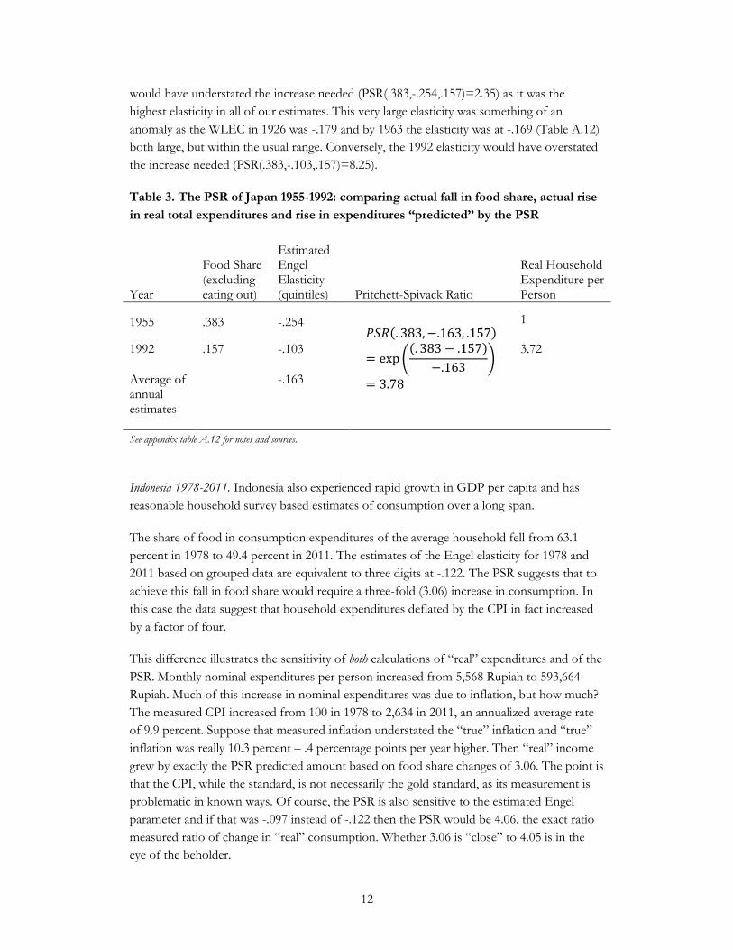
12

would have understated the increase needed (PSR(.383,-.254,.157)=2.35) as it was the

highest elasticity in all of our estimates. This very large elasticity was something of an

anomaly as the WLEC in 1926 was -.179 and by 1963 the elasticity was at -.169 (Table A.12)

both large, but within the usual range. Conversely, the 1992 elasticity would have overstated

the increase needed (PSR(.383,-.103,.157)=8.25).

Table 3. The PSR of Japan 1955-1992: comparing actual fall in food share, actual rise

in real total expenditures and rise in expenditures “predicted” by the PSR

Year

Food Share (excluding eating out)

Estimated Engel Elasticity (quintiles) Pritchett-Spivack Ratio

Real Household Expenditure per Person

1955 .383 -.254 (

((

)

1

1992 .157 -.103 3.72

Average of annual estimates

-.163

See appendix table A.12 for notes and sources.

Indonesia 1978-2011. Indonesia also experienced rapid growth in GDP per capita and has

reasonable household survey based estimates of consumption over a long span.

The share of food in consumption expenditures of the average household fell from 63.1

percent in 1978 to 49.4 percent in 2011. The estimates of the Engel elasticity for 1978 and

2011 based on grouped data are equivalent to three digits at -.122. The PSR suggests that to

achieve this fall in food share would require a three-fold (3.06) increase in consumption. In

this case the data suggest that household expenditures deflated by the CPI in fact increased

by a factor of four.

This difference illustrates the sensitivity of both calculations of “real” expenditures and of the

PSR. Monthly nominal expenditures per person increased from 5,568 Rupiah to 593,664

Rupiah. Much of this increase in nominal expenditures was due to inflation, but how much?

The measured CPI increased from 100 in 1978 to 2,634 in 2011, an annualized average rate

of 9.9 percent. Suppose that measured inflation understated the “true” inflation and “true”

inflation was really 10.3 percent – .4 percentage points per year higher. Then “real” income

grew by exactly the PSR predicted amount based on food share changes of 3.06. The point is

that the CPI, while the standard, is not necessarily the gold standard, as its measurement is

problematic in known ways. Of course, the PSR is also sensitive to the estimated Engel

parameter and if that was -.097 instead of -.122 then the PSR would be 4.06, the exact ratio

measured ratio of change in “real” consumption. Whether 3.06 is “close” to 4.05 is in the

eye of the beholder.

13

Table 4. The PSR of Indonesia 1978-2011: comparing actual fall in the food share,

actual rise in real total expenditures and rise in expenditures “predicted” by the PSR

Year

Food Share (excluding eating out)

Estimated Engel Elasticity Pritchett-Spivack Ratio

Real Household Expenditure per Person, CPI deflated (1978=1)

1978 .631 -.122 (

((

)

1

2011 .494 -.122 4.05

Source: authors calculations from Indonesia SUSENAS reports.

5. Applications

5.1 How much growth is needed?

The question this section seeks to answer is: “How much would the expenditures of the

typical (median) household in various countries need to increase to reach the food share of

the poor households in the OECD?” In a discussion of global development it can hardly be

contemplated that the typical person in every country is not at the very least to expect to

attain a similar array of choices of at least those enjoyed by the poor in the OECD today.

Perhaps the level of consumption of the rich in the OECD is neither achievable nor, in

some deep and higher sense, desirable. But it is hard to see how a “development” agenda

could not include a future which provides the typical person with at least the same chances

and choices that the poor in rich countries now enjoy.

In this section we do three things. First, we calculate the typical food share of households

that are considered “poor” in the OECD. Second, we use data from a variety of countries to

calculate the Pritchett-Spivack ratio of the median household in the ith country to the food

share of the OECD poor at various Engel elasticities7:

7 We might be concerned about the comparability of household food consumption data in developing countries, and household food consumption data in rich countries. In poor rural areas, households tend to grow a large portion of their own food. For households like these, surveyors must ask respondents to impute the value of food produced at home for personal consumption, a difficult calculation that may be imputed inaccurately or inconsistently across households and countries. Since households that produce their own food make up a much greater share of the population in developing countries, this inaccurate imputation may introduce some bias. However, when we compare the median food shares in urban and rural areas (see appendix table 14) we find that they are similar, which suggests that this type of systemic bias need not be a major concern.

14

(

Third, we then calculate how many years of rapid (e.g. 4 percent per annum) growth would

be needed for the typical household to reach the food share of the OECD poor.

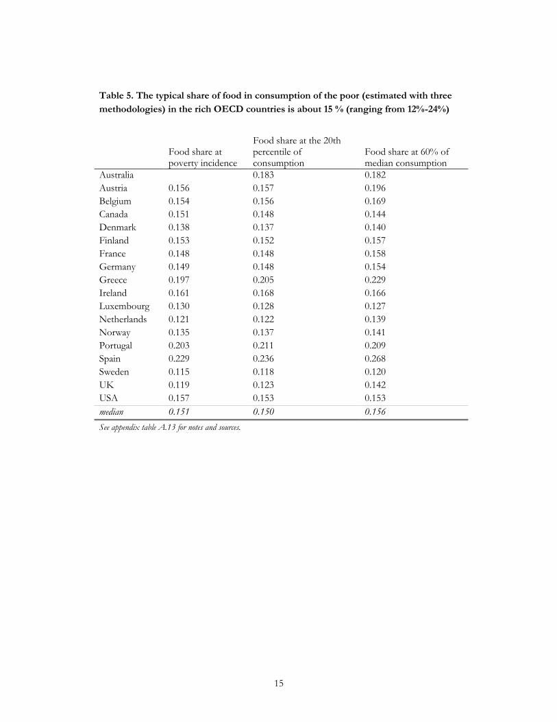
Food share of the rich OECD country poor. In Table 6 we calculate the food share of “the poor”

in rich OECD countries in three different ways. First we use food share data by quintile the

food share to interpolate the food share at the poverty rate in these countries. A second,

quick and dirty, calculation is to just calculate the food share at the 20th percentile. A third is

to adopt a common poverty definition as those at less than 60 percent of median

consumption. While each of these methods produces slightly different results for each

country, the typical food share for a “poor” household in a rich OECD country is very

robustly right around 15 percent.

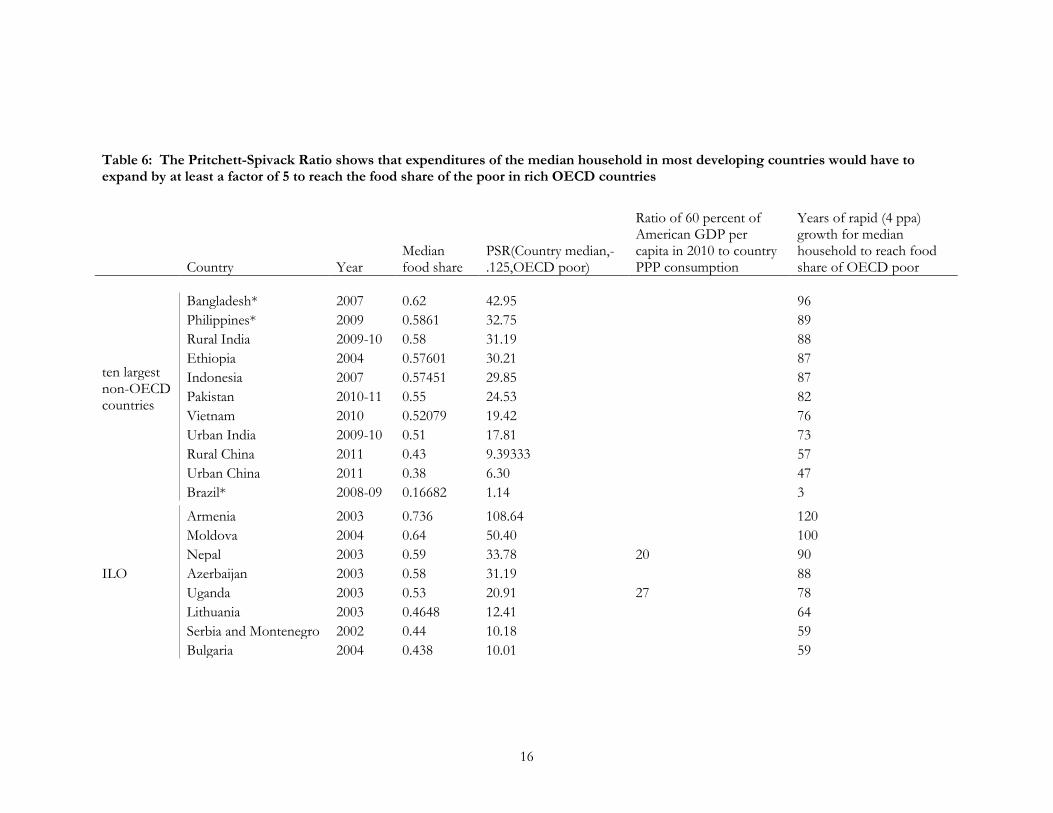
PSR of median in poor country to the rich OECD country poor. Table 6 shows the PSR calculations

for the collection of countries for which we had household data and hence could match

WLEC estimates with estimates of the PSR. We find that the PSR ratios show that, for the

typical (median) household to choose the same food share as that of the rich OECD country

poor the total expenditures in most poor countries would have to expand by at least an order of

magnitude. For countries where the current food share is one half or higher the PSR using a

WLEC of -.125 is over 15 (exp((.15-.5)/-.125))=exp(.35*8)=exp(2.8)≈16.4). Even for “upper

middle income” countries like Argentina and South Africa the PSR is over 5.

15

Table 5. The typical share of food in consumption of the poor (estimated with three

methodologies) in the rich OECD countries is about 15 % (ranging from 12%-24%)

Food share at poverty incidence

Food share at the 20th percentile of consumption

Food share at 60% of median consumption

Australia 0.183 0.182

Austria 0.156 0.157 0.196

Belgium 0.154 0.156 0.169

Canada 0.151 0.148 0.144

Denmark 0.138 0.137 0.140

Finland 0.153 0.152 0.157

France 0.148 0.148 0.158

Germany 0.149 0.148 0.154

Greece 0.197 0.205 0.229

Ireland 0.161 0.168 0.166

Luxembourg 0.130 0.128 0.127

Netherlands 0.121 0.122 0.139

Norway 0.135 0.137 0.141

Portugal 0.203 0.211 0.209

Spain 0.229 0.236 0.268

Sweden 0.115 0.118 0.120

UK 0.119 0.123 0.142

USA 0.157 0.153 0.153

median 0.151 0.150 0.156

See appendix table A.13 for notes and sources.

16

Table 6: The Pritchett-Spivack Ratio shows that expenditures of the median household in most developing countries would have to expand by at least a factor of 5 to reach the food share of the poor in rich OECD countries

Country Year Median food share

PSR(Country median,-.125,OECD poor)

Ratio of 60 percent of American GDP per capita in 2010 to country PPP consumption

Years of rapid (4 ppa) growth for median household to reach food share of OECD poor

ten largest non-OECD countries

Bangladesh* 2007 0.62 42.95

96

Philippines* 2009 0.5861 32.75

89

Rural India 2009-10 0.58 31.19

88

Ethiopia 2004 0.57601 30.21

87

Indonesia 2007 0.57451 29.85

87

Pakistan 2010-11 0.55 24.53

82

Vietnam 2010 0.52079 19.42

76

Urban India 2009-10 0.51 17.81

73

Rural China 2011 0.43 9.39333

57

Urban China 2011 0.38 6.30

47

Brazil* 2008-09 0.16682 1.14

3

ILO

Armenia 2003 0.736 108.64

120

Moldova 2004 0.64 50.40

100

Nepal 2003 0.59 33.78 20 90

Azerbaijan 2003 0.58 31.19

88

Uganda 2003 0.53 20.91 27 78

Lithuania 2003 0.4648 12.41

64

Serbia and Montenegro 2002 0.44 10.18

59

Bulgaria 2004 0.438 10.01

59

17

Belarus 2004 0.39 6.82

49

Latvia 2003 0.383 6.45

48

Argentina 1996 0.38 6.30 3.1 47

Iran, Is 2003 0.29 3.06 3.9 29

Turkey 2005 0.29 3.06 6 29

Macau 2002-03 0.263 2.47

23

Korea, R 2004 0.26 2.41 3 22

Hungary 2005 0.25 2.23 2.9 20

Malta 2005 0.21 1.62 2.2 12

Singapore 2004 0.19 1.38 2.1 8

Iceland 2001 0.17 1.17 1.6 4

Cyprus 2005 0.16 1.08 1.8 2

CLSP

Tajikistan 2003 0.71 88.87

114

Nepal 1996 0.63 46.01

98

Ghana 1998 0.62 41.50

95

Malawi 2004 0.61 40.84

95

Albania 2005 0.60 35.79

91

Nepal 2003 0.59 34.47

90

Vietnam 1997 0.58 31.29

88

Bulgaria 2001 0.56 25.70

83

Pakistan 1991 0.53 20.10

77

Ecuador 1998 0.51 17.84

73

Ecuador 1995 0.49 14.71

69

Guatemala 2000 0.49 14.61

68

Panama 2003 0.41 8.23

54

Bosnia 2001 0.36 5.16

42

18

LIS

Romania 1995 0.57 28.79

86

Guatemala 2006 0.45 11.02

61

Estonia 2000 0.43 9.39

57

Peru 2004 0.41 8.00

53

South Africa 2008 0.38 6.30

47

Hungary 1999 0.36 5.37

43

Poland 2004 0.32 3.90

35

Taiwan 2005 0.23 1.90

16

Ukraine 1995 0.2 1.49

10

Mexico 2004 0.2 1.49

10

Slovenia 2004 0.18 1.27

6

median 0.45 10.60 3.00 60.17

notes: ILO & country office medians are food share of median consumption group. LIS and CLSP data are median food share. *the national statistical agency does not report data by decile or quintile, so these food shares are the average of the middle income or consumption bracket reported. sources: see appendix tables A.1, A.2, A.3, A.4, A.5, and A.6.

19

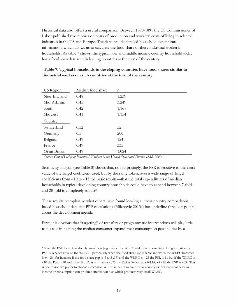
Historical data also offers a useful comparison. Between 1890-1891 the US Commissioner of

Labor published two reports on costs of production and workers’ costs of living in selected

industries in the US and Europe. The data include detailed household expenditure

information, which allows us to calculate the food share of these industrial worker’s

households. As table 7 shows, the typical, low and middle income country household today

has a food share last seen in leading countries at the turn of the century.

Table 7. Typical households in developing countries have food shares similar to

industrial workers in rich countries at the turn of the century

US Region

Median food share n New England

0.48 1,239

Mid-Atlantic

0.45 3,249 South

0.42 1,167

Midwest

0.41 1,154

Country Switzerland

0.52 52 Germany

0.5 200

Belgium

0.49 124 France

0.49 335

Great Britain

0.49 1,024 Source: Cost of Living of Industrial Workers in the United States and Europe 1888-1890.

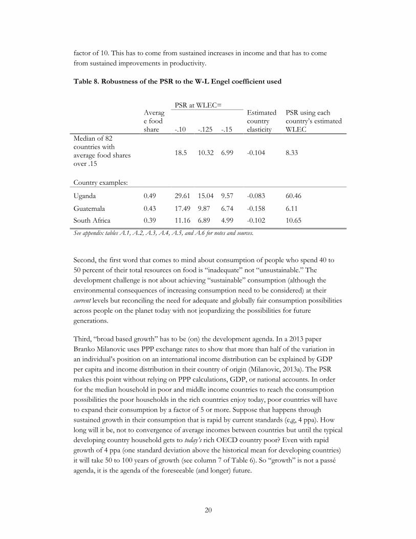
Sensitivity analysis (see Table 8) shows that, not surprisingly, the PSR is sensitive to the exact

value of the Engel coefficient used, but by the same token, over a wide range of Engel

coefficients from -.10 to -.15 the basic results—that the total expenditures of median

households in typical developing country households could have to expand between 7-fold

and 20-fold is completely robust8.

These results reemphasize what others have found looking at cross-country comparisons

based household data and PPP calculations (Milanovic 2013a) but underline three key points

about the development agenda.

First, it is obvious that “targeting” of transfers or programmatic interventions will play little

to no role in helping the median consumer expand their consumption possibilities by a

8 Since the PSR formula is doubly non-linear (e.g. divided by WLEC and then exponentiated to get a ratio) the

PSR is very sensitive to the WLEC—particularly when the food share gap is large and when the WLEC becomes

low. So, for instance if the food share gap is .3 (.45-.15) and the WLEC is .125 the PSR is 11 but if the WLEC is

-.10 the PSR is 20 and if the WLEC is as small as -.075 the PSR is 54 and at a WLEC of -.05 the PSR is 403. This

is one reason we prefer to choose a common WLEC rather than country by country as measurement error in

income or consumption can produce attenuation bias which produces very small WLEC.

20

factor of 10. This has to come from sustained increases in income and that has to come

from sustained improvements in productivity.

Table 8. Robustness of the PSR to the W-L Engel coefficient used

Average food share

PSR at WLEC= Estimated country elasticity

PSR using each country’s estimated WLEC -.10 -.125 -.15

Median of 82 countries with average food shares over .15

18.5 10.32 6.99 -0.104 8.33

Country examples:

Uganda 0.49 29.61 15.04 9.57 -0.083 60.46

Guatemala 0.43 17.49 9.87 6.74 -0.158 6.11

South Africa 0.39 11.16 6.89 4.99 -0.102 10.65

See appendix tables A.1, A.2, A.3, A.4, A.5, and A.6 for notes and sources.

Second, the first word that comes to mind about consumption of people who spend 40 to

50 percent of their total resources on food is “inadequate” not “unsustainable.” The

development challenge is not about achieving “sustainable” consumption (although the

environmental consequences of increasing consumption need to be considered) at their

current levels but reconciling the need for adequate and globally fair consumption possibilities

across people on the planet today with not jeopardizing the possibilities for future

generations.

Third, “broad based growth” has to be (on) the development agenda. In a 2013 paper

Branko Milanovic uses PPP exchange rates to show that more than half of the variation in

an individual’s position on an international income distribution can be explained by GDP

per capita and income distribution in their country of origin (Milanovic, 2013a). The PSR

makes this point without relying on PPP calculations, GDP, or national accounts. In order

for the median household in poor and middle income countries to reach the consumption

possibilities the poor households in the rich countries enjoy today, poor countries will have

to expand their consumption by a factor of 5 or more. Suppose that happens through

sustained growth in their consumption that is rapid by current standards (e,g, 4 ppa). How

long will it be, not to convergence of average incomes between countries but until the typical

developing country household gets to today’s rich OECD country poor? Even with rapid

growth of 4 ppa (one standard deviation above the historical mean for developing countries)

it will take 50 to 100 years of growth (see column 7 of Table 6). So “growth” is not a passé

agenda, it is the agenda of the foreseeable (and longer) future.

21

5.2 Are the “rich” in poor countries rich?

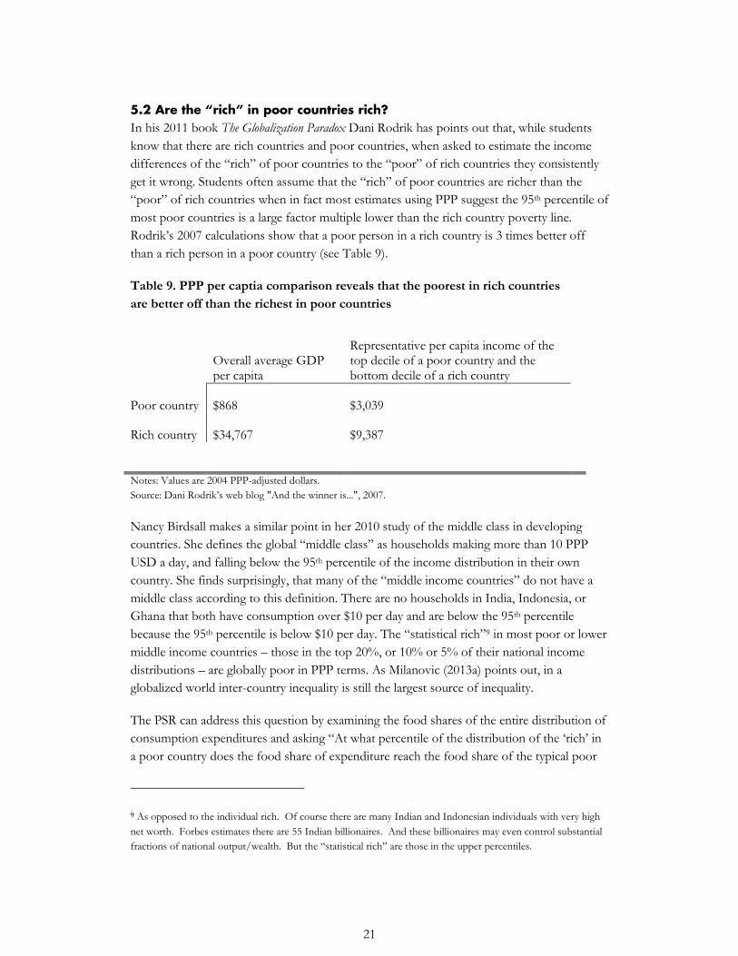
In his 2011 book The Globalization Paradox Dani Rodrik has points out that, while students

know that there are rich countries and poor countries, when asked to estimate the income

differences of the “rich” of poor countries to the “poor” of rich countries they consistently

get it wrong. Students often assume that the “rich” of poor countries are richer than the

“poor” of rich countries when in fact most estimates using PPP suggest the 95th percentile of

most poor countries is a large factor multiple lower than the rich country poverty line.

Rodrik’s 2007 calculations show that a poor person in a rich country is 3 times better off

than a rich person in a poor country (see Table 9).

Table 9. PPP per captia comparison reveals that the poorest in rich countries

are better off than the richest in poor countries

Overall average GDP per capita

Representative per capita income of the top decile of a poor country and the bottom decile of a rich country

Poor country $868 $3,039

Rich country $34,767 $9,387

Notes: Values are 2004 PPP-adjusted dollars.

Source: Dani Rodrik’s web blog "And the winner is...", 2007.

Nancy Birdsall makes a similar point in her 2010 study of the middle class in developing

countries. She defines the global “middle class” as households making more than 10 PPP

USD a day, and falling below the 95th percentile of the income distribution in their own

country. She finds surprisingly, that many of the “middle income countries” do not have a

middle class according to this definition. There are no households in India, Indonesia, or

Ghana that both have consumption over $10 per day and are below the 95th percentile

because the 95th percentile is below $10 per day. The “statistical rich”9 in most poor or lower

middle income countries – those in the top 20%, or 10% or 5% of their national income

distributions – are globally poor in PPP terms. As Milanovic (2013a) points out, in a

globalized world inter-country inequality is still the largest source of inequality.

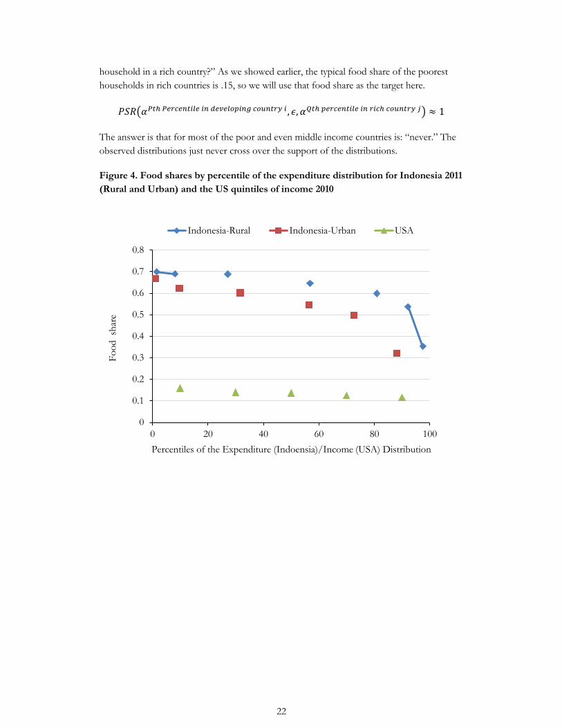
The PSR can address this question by examining the food shares of the entire distribution of

consumption expenditures and asking “At what percentile of the distribution of the ‘rich’ in

a poor country does the food share of expenditure reach the food share of the typical poor

9 As opposed to the individual rich. Of course there are many Indian and Indonesian individuals with very high

net worth. Forbes estimates there are 55 Indian billionaires. And these billionaires may even control substantial

fractions of national output/wealth. But the “statistical rich” are those in the upper percentiles.

22

household in a rich country?” As we showed earlier, the typical food share of the poorest

households in rich countries is .15, so we will use that food share as the target here.

( )

The answer is that for most of the poor and even middle income countries is: “never.” The

observed distributions just never cross over the support of the distributions.

Figure 4. Food shares by percentile of the expenditure distribution for Indonesia 2011

(Rural and Urban) and the US quintiles of income 2010

0

0.1

0.2

0.3

0.4

0.5

0.6

0.7

0.8

0 20 40 60 80 100

Fo

od sh

are

Percentiles of the Expenditure (Indoensia)/Income (USA) Distribution

Indonesia-Rural Indonesia-Urban USA

23

Figure 5. Food shares by deciles of consumption for India 2009-2010 and the US by

income quintiles 2010.

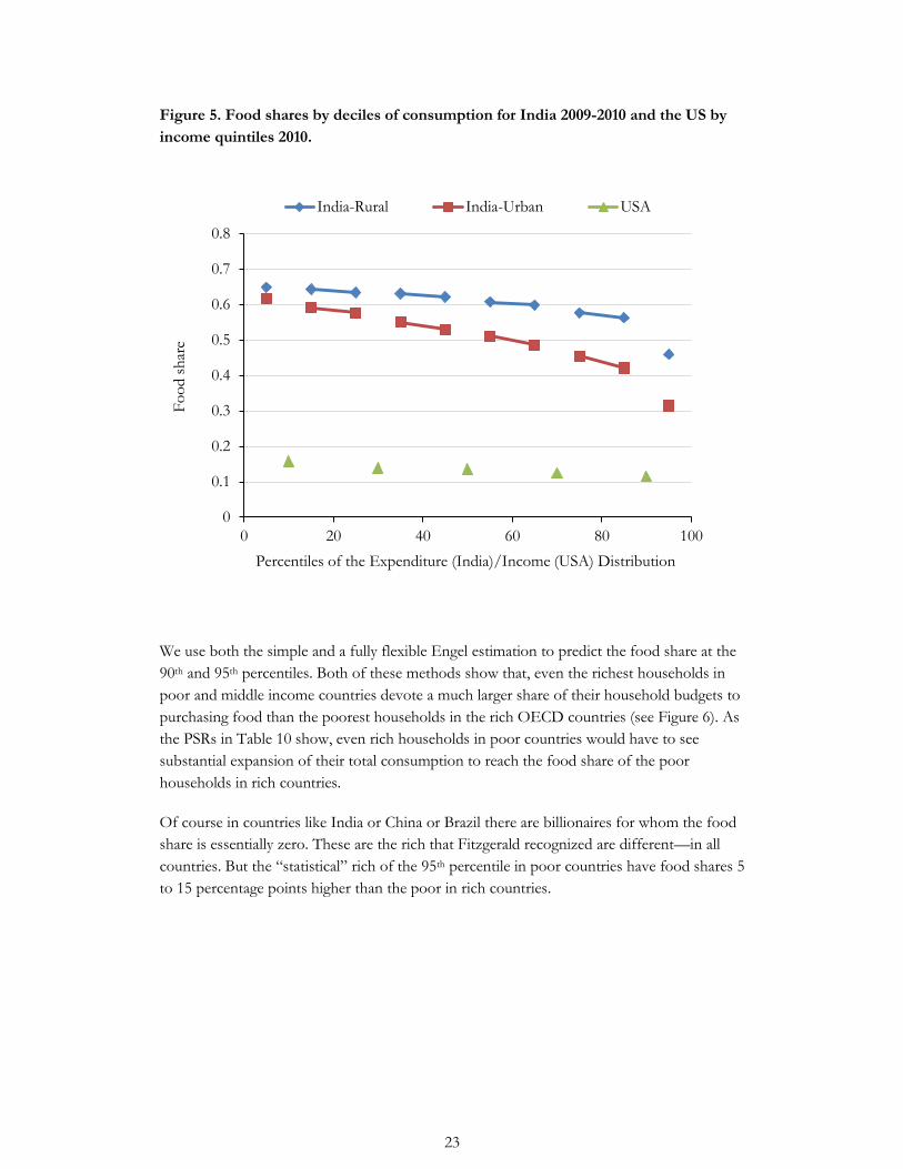
We use both the simple and a fully flexible Engel estimation to predict the food share at the

90th and 95th percentiles. Both of these methods show that, even the richest households in

poor and middle income countries devote a much larger share of their household budgets to

purchasing food than the poorest households in the rich OECD countries (see Figure 6). As

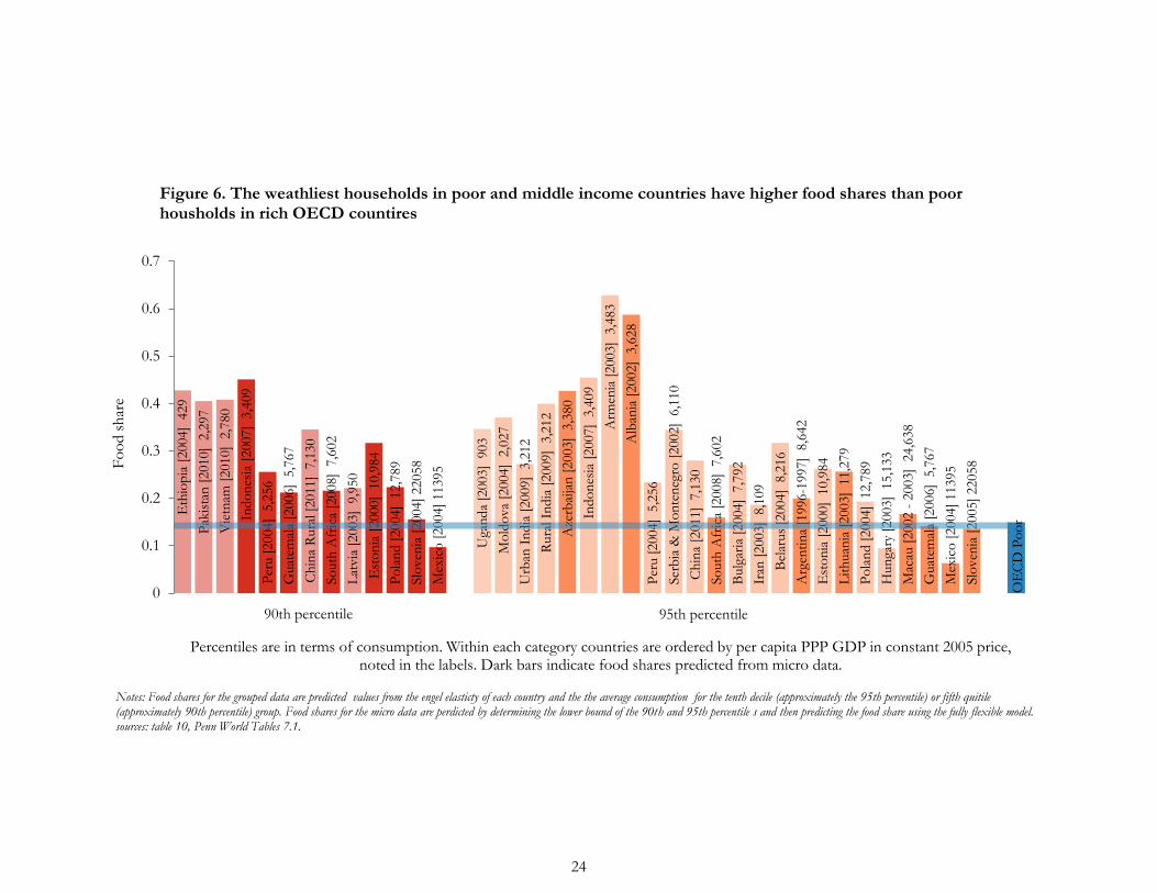
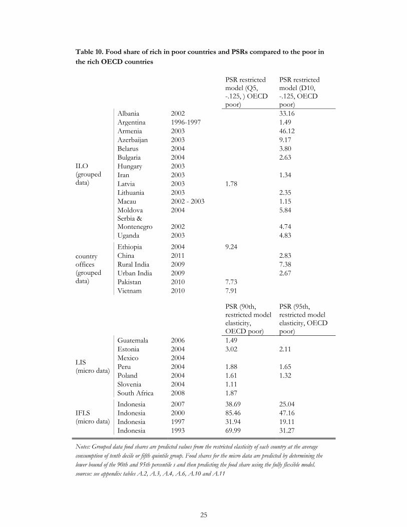
the PSRs in Table 10 show, even rich households in poor countries would have to see

substantial expansion of their total consumption to reach the food share of the poor

households in rich countries.

Of course in countries like India or China or Brazil there are billionaires for whom the food

share is essentially zero. These are the rich that Fitzgerald recognized are different—in all

countries. But the “statistical” rich of the 95th percentile in poor countries have food shares 5

to 15 percentage points higher than the poor in rich countries.

0

0.1

0.2

0.3

0.4

0.5

0.6

0.7

0.8

0 20 40 60 80 100

India-Rural India-Urban USA

Fo

od

sh

are

Percentiles of the Expenditure (India)/Income (USA) Distribution

24

Eth

iop

ia [

2004]

429

Pak

ista

n [

2010]

2,2

97

Vie

tnam

[2010]

2,7

80

Ind

on

esia

[2007]

3,4

09

Per

u [

2004]

5,2

56

Guat

emal

a [2

006]

5,7

67

Ch

ina

Rura

l [2

011]

7,1

30

So

uth

Afr

ica

[2008]

7,6

02

Lat

via

[2003]

9,9

50

Est

on

ia [

2000]

10,9

84

Po

lan

d [

2004]

12,7

89

Slo

ven

ia [

2004]

22058

Mex

ico

[2004]

11395

Uga

nd

a [2

003]

903

Mo

ldo

va

[2004]

2,0

27

Urb

an I

nd

ia [

2009]

3,2

12

Rura

l In

dia

[2009]

3,2

12

Aze

rbai

jan

[2003]

3,3

80

Ind

on

esia

[2007]

3,4

09

Arm

enia

[2003]

3,4

83

Alb

ania

[2002]

3,6

28

Per

u [

2004]

5,2

56

Ser

bia

& M

on

ten

egro

[2002]

6,1

10

Ch

ina

[2011]

7,1

30

So

uth

Afr

ica

[2008]

7,6

02

Bulg

aria

[2004]

7,7

92

Iran

[2003]

8,1

09

Bel

arus

[2004]

8,2

16

Arg

enti

na

[1996-1

997]

8,6

42

Est

on

ia [

2000]

10,9

84

Lit

huan

ia [

2003]

11,2

79

Po

lan

d [

2004]

12,7

89

Hun

gary

[2003]

15,1

33

Mac

au [

2002 -

2003]

24,6

38

Guat

emal

a [2

006]

5,7

67

Mex

ico

[2004]

11395

Slo

ven

ia [

2005]

22058

0

0.1

0.2

0.3

0.4

0.5

0.6

0.7

Figure 6. The weathliest households in poor and middle income countries have higher food shares than poor housholds in rich OECD countires

Fo

od s

har

e

90th percentile 95th percentile

Percentiles are in terms of consumption. Within each category countries are ordered by per capita PPP GDP in constant 2005 price, noted in the labels. Dark bars indicate food shares predicted from micro data.

OE

CD

Po

or

Notes: Food shares for the grouped data are predicted values from the engel elasticty of each country and the the average consumption for the tenth decile (approximately the 95th percentile) or fifth quitile (approximately 90th percentile) group. Food shares for the micro data are perdicted by determining the lower bound of the 90th and 95th percentile s and then predicting the food share using the fully flexible model. sources: table 10, Penn World Tables 7.1.

25

Table 10. Food share of rich in poor countries and PSRs compared to the poor in

the rich OECD countries

PSR restricted model (Q5, -.125, ) OECD poor)

PSR restricted model (D10, -.125, OECD poor)

ILO (grouped data)

Albania 2002

33.16

Argentina 1996-1997

1.49

Armenia 2003

46.12

Azerbaijan 2003

9.17

Belarus 2004

3.80

Bulgaria 2004

2.63

Hungary 2003 Iran 2003

1.34

Latvia 2003 1.78 Lithuania 2003

2.35

Macau 2002 - 2003

1.15

Moldova 2004

5.84 Serbia & Montenegro 2002

4.74

Uganda 2003

4.83

country offices (grouped data)

Ethiopia 2004 9.24 China 2011

2.83

Rural India 2009

7.38

Urban India 2009

2.67

Pakistan 2010 7.73 Vietnam 2010 7.91

PSR (90th, restricted model elasticity, OECD poor)

PSR (95th, restricted model elasticity, OECD poor)

LIS (micro data)

Guatemala 2006 1.49 Estonia 2004 3.02 2.11

Mexico 2004 Peru 2004 1.88 1.65

Poland 2004 1.61 1.32

Slovenia 2004 1.11 South Africa 2008 1.87

IFLS (micro data)

Indonesia 2007 38.69 25.04

Indonesia 2000 85.46 47.16

Indonesia 1997 31.94 19.11

Indonesia 1993 69.99 31.27

Notes: Grouped data food shares are predicted values from the restricted elasticity of each country at the average

consumption of tenth decile or fifth quintile group. Food shares for the micro data are predicted by determining the

lower bound of the 90th and 95th percentile s and then predicting the food share using the fully flexible model.

sourcse: see appendix tables A.2, A.3, A.4, A.6, A.10 and A.11

26

6. Conclusion

Although the bulk of this paper is narrow and technical, we are making a broad and

important point that is relevant to current discussions about the post-2015 development

agenda. Strangely, in spite of the fact that the typical person in the developing world has a

level of consumption possibilities that is roughly an order of magnitude lower than the poor in

rich countries, the need for sustained growth in material standard of living of the typical

person in the developing world is not the dominant theme of these discussions.

Intriguingly, the word seemingly most frequently modifying the desirable type of

“consumption” is not “higher” but “sustainable.” But who wants to merely “sustain” their

current levels of consumption? This might be a goal for the world’s doubly rich (rich in rich

countries) whose consumption they might regard as high enough. However, from their

current levels, the material possibilities of the typical individual in a typical poor country

would have to grow at their recent pace for 100 years before they would enjoy the

consumption possibilities that the current poor in rich countries enjoy today. We argue word

that should be most associated with “consumption” is “inadequate” and the word that

should be most associated with “growth” is “rapid.”10

Moreover, there is a steady increase in the attention to inequality within countries as a

development issue. There is a general sense among rich country residents and tax payers that

“the rich” in poor countries are doing well, even better than “the poor” in rich countries and

hence if resources could just be redistributed from “the rich” to “the poor” within poor

countries that problems of poverty could be solved. As we show, almost nothing could be

further from the truth. Of course, poor countries have a comparatively handful of the

globally super-rich, but the richest 10% in poor countries have a food share that is typically

double that of the poor in the rich OECD countries — suggesting the material standard of

living of the poor in the OECD is three times as high as that of the rich in “middle income”

countries like India or Indonesia.

10 This is not to say that growth of GDP is itself a goal, it is just a means to the end of higher human well-being.

But one can take any measure of well-being and expanding the productivity of individuals will be essential to

broad based improvements in that measure.

27

References

“10-8 Per Capita Annual Cash Living Expenditure of Urban Households by Income

Percentile.” Government. China Statistical Yearbook 2011, 2011.

http://www.stats.gov.cn/tjsj/ndsj/2011/indexeh.htm.

Almas, Ingvild. “International Income Inequality: Measuring PPP Bias by Estimating Engel

Curves for Food.” American Economic Review, 102(2): 1093-1117 (2012).

Alan Heston, Robert Summers and Bettina Aten, Penn World Table Version 7.1, Center for

International Comparisons of Production, Income and Prices at the University of

Pennsylvania, Nov 2012

Alan Heston, Robert Summers and Bettina Aten, Penn World Table Version 7.0, Center for

International Comparisons of Production, Income and Prices at the University of

Pennsylvania, June 2011.

Anker, Richard. “Engel’s Law Around the World 150 Years Later.” Political Economy

Research Institute (2011).

http://www.peri.umass.edu/fileadmin/pdf/working_papers/working_papers_201-

250/WP247.pdf.

Birdsall, Nancy. “The (Indispensable) Middle Class.” Center for Global Development

Working Paper Series (2010).

“Chapter 20 Family Income and Expenditure, Tables 20-6, 20-7-b,and 20-7-c.” Ministry of

Internal Affaris and Communications, n.d.

http://www.stat.go.jp/english/data/chouki/20.htm.

Collier, Paul. The Bottom Billion. New York: Oxford University Press, 2007.

Deaton, Angus, Jed Friedman, and Alatas Vivi. “Purchasing Power Parity Exchange Rates

from Household Survey Data: India and Indonesia” (2004).

http://www.princeton.edu/~deaton/downloads/PPP_Exchange_rates_may04_relabele

d_mar11.pdf.

“Detailed Tables of HIES 2010.” Government. Bangladesh Bureau of Statistics, 2010.

http://www.bbs.gov.bd/PageWebMenuContent.aspx?MenuKey=320.

“Household Integrated Economic Survey (HIES) 2010-11.” Accessed June 11, 2013.

http://www.pbs.gov.pk/content/household-integrated-economic-survey-hies-2010-11.

Houthakker, H.S. “An International Comparison of Households Expenditure Patters,

Commemorating the Century of Engel’s Law.” Econometrica 25, no. 4 (1957).

General Statistics Office. Results of the Viet Nam Household Living Standards Survey 2010.

Statistical Publishing House, 2010.

Ghani, Ejaz. The Poor Half Billion in South Asia: What Is Holding Back Lagging Regions?

OUP Catalogue. Oxford University Press, 2010.

http://econpapers.repec.org/bookchap/oxpobooks/9780198068846.htm.

Inglehart, Ronald. Modernization and Postmodernization: Cultural, Economic, and Polt ical

Change in 43 Societies. Princeton University Press, 1997.

International Labor Organization. “HIES - Houshold Income and Expenditure Statistics.”

Data portal. LABORSTA Internet, n.d. http://laborsta.ilo.org/STP/guest.

28

Kenny, Charles, and Lant Pritchett. “Promoting Millennium Development Ideals: The Risks

of Defining Development Down” (2013).

Leser, C. “Forms of Engel Functions.” Econometrica 31 (1963): 694–703.

Milanovic, Branko. “Global Inequaltiy of Opportunity: How Much of Our Income Is

Determined by Where We Live?” Unpublished (2013a).

Milanovic, Branko. “The Inequality Possibility Frontier : Extensions and New Applications.”

Policy Research Working Paper (2013b).

National Statistical Organization, National Sample Survey Office, Ministry of Statistics and

Programme Implementation Government of India. Key Indicators of Household

Consumer Expenditure in India 2009-2010, 2011.

“Pesquisa Nacional Por Amostra De Domicílios.” Government. Instituto Brasileiro De

Geografia e Estatística, n.d. http://www.sidra.ibge.gov.br/pnad/default.asp.

Republic of the Philippines National Statistics Office. “2009 FIES (Additional Tables).”

Accessed June 11, 2013. http://www.census.gov.ph/content/2009-fies-additional-

tables.

Rodrik, Dani. The Globalization Paradox: Democracy and the Future of the World

Economy. W. W. Norton & Company, 2011.

———. “And the Winner Is...” Dani Rodrik’s Weblog, May 5, 2007.

http://rodrik.typepad.com/dani_rodriks_weblog/2007/05/and_the_winner_.html.

Statistics Indonesia. Expenditures for Consumption of Indonesia. Statistics Indoensia, 2011.

The Federal Democratic Republic of Ethiopia Central Statistics Agency. Household Income

Consumption and Expenditure (HICE) Survey 2004/5 Volume I, n.d.

Working, H. “Statistical Laws of Family Expenditures.” Journal of the American Statistical

Association 38 (1943): 43–56

29

Appendix

A.1 Comparative Living Statistics Project - WLEC estimates, average food share & PSR

Elasticity Absolute value of t R2 n

Mean food share

PSR (country avg, -.1, OECD poor)

PSR (country avg, -.125, OECD poor)

PSR (country avg, -.15, OECD poor)

PSR (country avg, country elasticity, OECD poor)

Albania 2002 -0.0438 32.35*** 0.0381 3,599 0.67 186.047 65.418 32.590 150089.819

Albania 2005 -0.0646 32.56*** 0.0684 3,638 0.59 79.998 33.301 18.566 887.613

Albania 1996 -0.0999 29.49*** 0.1648 1,503 0.6 88.323 36.046 19.833 88.632

Bulgaria 2001 -0.1034 40.01*** 0.1242 2,500 0.56 62.302 27.265 15.716 54.295

Bulgaria 1995 -0.0317 22.10*** 0.0173 2,460 0.62 111.609 43.467 23.181 2901848.339

Bosnia 2001 -0.0479 28.01*** 0.0384 5,400 0.34 8.029 5.293 4.010 77.627

Ecuador 1995 -0.1152 54.95*** 0.2298 5,661 0.48 26.549 13.780 8.900 17.216

Ecuador 1998 -0.1207 64.26*** 0.2949 5,693 0.49 30.265 15.302 9.712 16.883

Ghana 1987 -0.0207 30.17*** 0.0119 3,104 0.70 250.636 83.030 39.752 398314299913.121

Ghana 1988 -0.0348 32.41*** 0.0314 3,181 0.67 181.817 64.225 32.094 3077285.357

Ghana 1991 -0.0528 39.58*** 0.0652 4,523 0.61 99.683 39.710 21.499 6118.343

Ghana 1998 -0.0340 39.46*** 0.0377 5,998 0.60 93.691 37.788 20.628 625475.877

Guatemala 2000 -0.0990 100.56*** 0.3034 7,276 0.48 27.113 14.013 9.025 28.072

Malawi 2004 -0.0345 62.41*** 0.0296 11,280 0.61 94.917 38.183 20.808 529011.672

Nepal 2003 -0.1922 98.54*** 0.5578 3,912 0.56 59.086 26.133 15.170 8.348

Nepal 1996 -0.1591 75.19*** 0.4016 3,373 0.6 85.370 35.079 19.388 16.372

Pakistan 1991 -0.0940 53.87*** 0.1462 4,794 0.52 39.805 19.053 11.658 50.362

Panama 2003 -0.1320 115.29*** 0.4325 6,363 0.43 16.412 9.378 6.458 8.331

Panama 1997 -0.1109 102.59*** 0.3794 4,938 0.47 24.288 12.833 8.387 17.762

Tajikistan 2003 -0.0552 64.94*** 0.0528 4,136 0.7 221.628 75.249 36.623 17607.785

Vietnam 1992 -0.1405 69.26*** 0.3443 4,799 0.62 105.214 41.463 22.287 27.464

Vietnam 1997 -0.1572 92.91*** 0.4629 5,999 0.57 65.694 28.446 16.281 14.340

Median -0.0965 82.684 34.190 18.977 65.961

Standard dev

0.0493

Source: World Bank Comparative Living Statistics Project. *** p<0.001, ** p<0.01, * p<0.05

30

A.2 Indonesia Family Life Survey - WLEC estimates, average food share & PSR

Elasticity Absolute value of t R2 n

Mean food share

PSR (country average, -.1, OECD poor)

PSR (country average, -.125, OECD poor)

PSR (country average, -.15, OECD poor)

PSR (country average, country own elasticity, OECD poor)

2007 -0.0824 44.30*** 0.134 12,658 0.56

61.286 26.909 15.544 147.615

2000 -0.0824 40.68*** 0.139 10,229 0.60

85.915 35.258 19.471 222.418

1997 -0.0942 40.41*** 0.178 7,536 0.57

65.463 28.366 16.243 84.686

1993 -0.0747 30.95*** 0.118 7,136 0.56

62.505 27.336 15.750 253.613

Median -0.0824

63.984 27.851 15.996 185.016

Notes: The RAND cooperation provides access to cleaned standardized data files of these data. Estimates are based on this micro data analysis. Source: Indonesia Family Life Survey (IFLS). *** p<0.001, ** p<0.01, * p<0.05

31

A.3 LIS - WLEC estimates, average food share & PSR

Country Year Elasticity Absolute value t R2 n

Mean food share

PSR (country average, -.1, OECD poor)

PSR (country average, -.125, OECD poor)

PSR (country average, -.15, OECD poor)

PSR (country average, country own elasticity, OECD poor)

Israel 2005 -0.0642 201.99 0.4958 41,492 0.160

France 2005 -0.0650 43.67 0.157 10,240 0.170

1.221 1.173 1.142 1.359

Germany 1983 -0.0627 89.72 0.1584 42,752 0.201

1.659 1.499 1.401 2.243

Slovenia 2004 -0.0567 20.26 0.0993 3,725 0.201

1.659 1.499 1.402 2.443

Ukraine 1995 -0.0935 63.15 0.3713 6,755 0.216

1.929 1.692 1.550 2.020

Mexico 2004 -0.0983 126.4 0.4142 22,595 0.223

2.083 1.799 1.631 2.109

Taiwan 2005 -0.1044 93.4 0.3894 13,681 0.237

2.398 2.013 1.791 2.311

Italy 2000 -0.1233 39.03 0.16 8,001 0.305

4.706 3.452 2.808 3.513

Poland 2004 -0.1555 160.34 0.4439 32,214 0.346

7.066 4.779 3.682 3.515

Spain 1980 -0.1512 108.6 0.3298 23,972 0.381

10.114 6.367 4.677 4.618 South Africa 2008 -0.1020 64.71 0.3648 7,291 0.391

11.163 6.890 4.995 10.645

Hungry 1999 -0.1240 10.83 0.0739 1,472 0.393

11.354 6.984 5.052 7.097

Peru 2004 -0.1672 100.55 0.3543 18,432 0.415

14.142 8.325 5.848 4.879

Guatemala 2006 -0.1581 131.89 0.5601 13,664 0.436

17.493 9.870 6.739 6.114

Estonia 2000 -0.1509 45.17 0.2671 5,601 0.444

18.872 10.487 7.088 7.008

Romania 1995 -0.1796 129.59 0.3472 31,571 0.574

69.162 29.641 16.849 10.573

Median -0.1138

7.066 4.779 3.682 3.515

Standard dev

0.0411

Notes: *** p<0.001, ** p<0.01, * p<0.05 Source: Luxembourg Income Study.

32

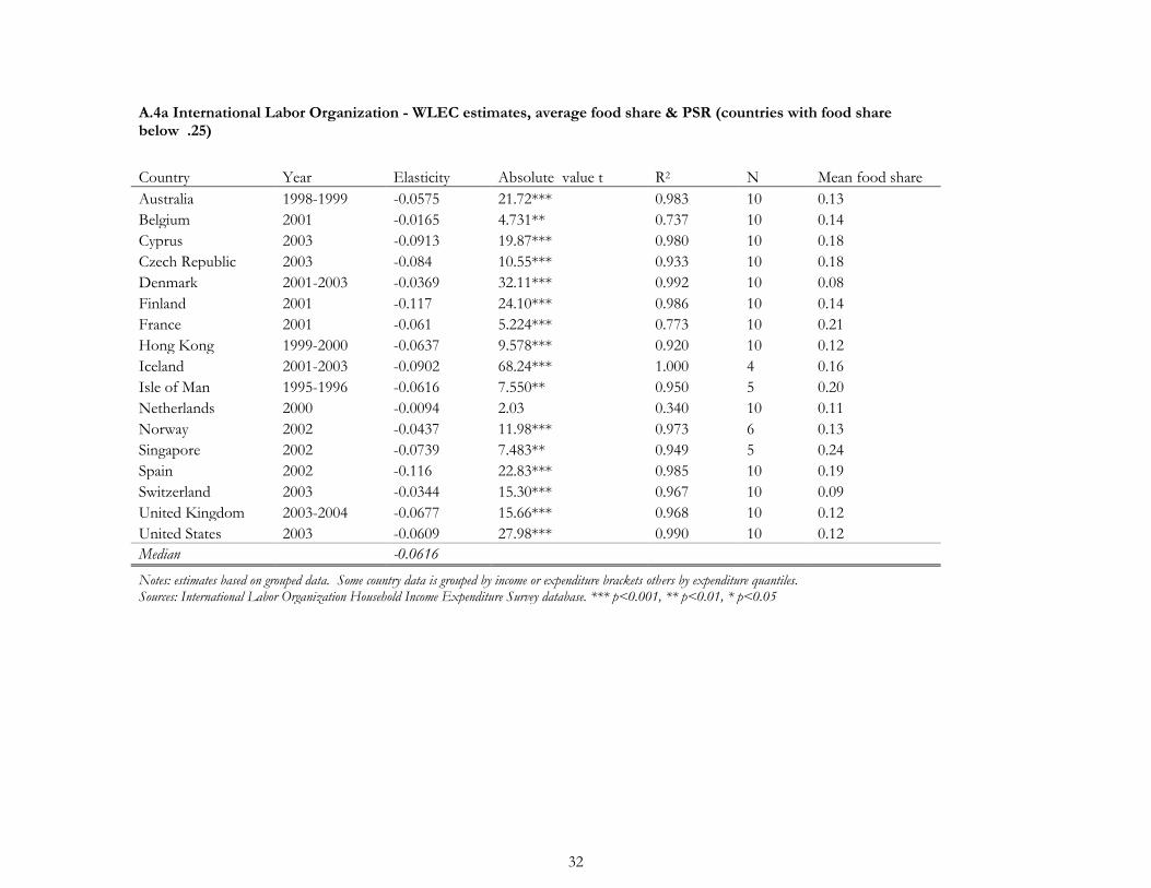
A.4a International Labor Organization - WLEC estimates, average food share & PSR (countries with food share below .25)

Country Year Elasticity Absolute value t R2 N Mean food share

Australia 1998-1999 -0.0575 21.72*** 0.983 10 0.13

Belgium 2001 -0.0165 4.731** 0.737 10 0.14

Cyprus 2003 -0.0913 19.87*** 0.980 10 0.18

Czech Republic 2003 -0.084 10.55*** 0.933 10 0.18

Denmark 2001-2003 -0.0369 32.11*** 0.992 10 0.08

Finland 2001 -0.117 24.10*** 0.986 10 0.14

France 2001 -0.061 5.224*** 0.773 10 0.21

Hong Kong 1999-2000 -0.0637 9.578*** 0.920 10 0.12

Iceland 2001-2003 -0.0902 68.24*** 1.000 4 0.16

Isle of Man 1995-1996 -0.0616 7.550** 0.950 5 0.20

Netherlands 2000 -0.0094 2.03 0.340 10 0.11

Norway 2002 -0.0437 11.98*** 0.973 6 0.13

Singapore 2002 -0.0739 7.483** 0.949 5 0.24

Spain 2002 -0.116 22.83*** 0.985 10 0.19

Switzerland 2003 -0.0344 15.30*** 0.967 10 0.09

United Kingdom 2003-2004 -0.0677 15.66*** 0.968 10 0.12

United States 2003 -0.0609 27.98*** 0.990 10 0.12

Median -0.0616

Notes: estimates based on grouped data. Some country data is grouped by income or expenditure brackets others by expenditure quantiles. Sources: International Labor Organization Household Income Expenditure Survey database. *** p<0.001, ** p<0.01, * p<0.05

33

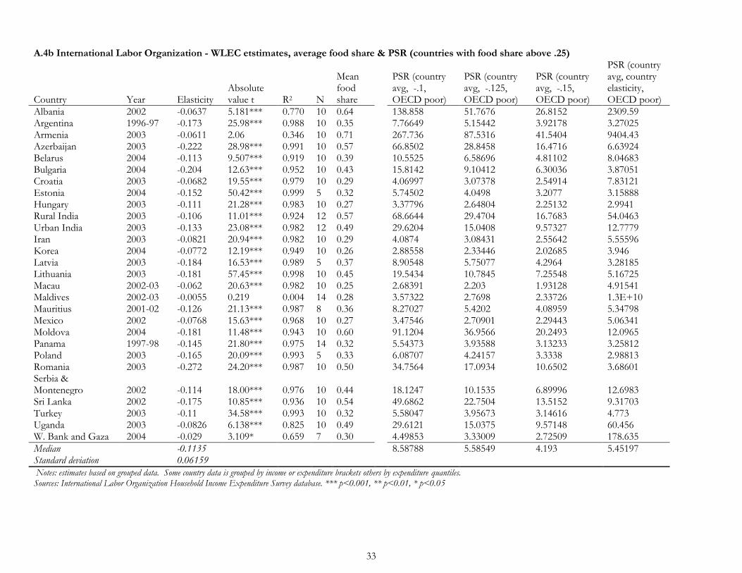
A.4b International Labor Organization - WLEC etstimates, average food share & PSR (countries with food share above .25)

Country Year Elasticity

Absolute value t R2 N

Mean food share

PSR (country avg, -.1, OECD poor)

PSR (country avg, -.125, OECD poor)

PSR (country avg, -.15, OECD poor)

PSR (country avg, country elasticity, OECD poor)

Albania 2002 -0.0637 5.181*** 0.770 10 0.64

138.858 51.7676 26.8152 2309.59 Argentina 1996-97 -0.173 25.98*** 0.988 10 0.35

7.76649 5.15442 3.92178 3.27025

Armenia 2003 -0.0611 2.06 0.346 10 0.71

267.736 87.5316 41.5404 9404.43 Azerbaijan 2003 -0.222 28.98*** 0.991 10 0.57

66.8502 28.8458 16.4716 6.63924

Belarus 2004 -0.113 9.507*** 0.919 10 0.39

10.5525 6.58696 4.81102 8.04683 Bulgaria 2004 -0.204 12.63*** 0.952 10 0.43

15.8142 9.10412 6.30036 3.87051

Croatia 2003 -0.0682 19.55*** 0.979 10 0.29

4.06997 3.07378 2.54914 7.83121 Estonia 2004 -0.152 50.42*** 0.999 5 0.32

5.74502 4.0498 3.2077 3.15888

Hungary 2003 -0.111 21.28*** 0.983 10 0.27

3.37796 2.64804 2.25132 2.9941 Rural India 2003 -0.106 11.01*** 0.924 12 0.57

68.6644 29.4704 16.7683 54.0463

Urban India 2003 -0.133 23.08*** 0.982 12 0.49

29.6204 15.0408 9.57327 12.7779 Iran 2003 -0.0821 20.94*** 0.982 10 0.29

4.0874 3.08431 2.55642 5.55596

Korea 2004 -0.0772 12.19*** 0.949 10 0.26

2.88558 2.33446 2.02685 3.946 Latvia 2003 -0.184 16.53*** 0.989 5 0.37

8.90548 5.75077 4.2964 3.28185

Lithuania 2003 -0.181 57.45*** 0.998 10 0.45

19.5434 10.7845 7.25548 5.16725 Macau 2002-03 -0.062 20.63*** 0.982 10 0.25

2.68391 2.203 1.93128 4.91541

Maldives 2002-03 -0.0055 0.219 0.004 14 0.28

3.57322 2.7698 2.33726 1.3E+10 Mauritius 2001-02 -0.126 21.13*** 0.987 8 0.36

8.27027 5.4202 4.08959 5.34798

Mexico 2002 -0.0768 15.63*** 0.968 10 0.27

3.47546 2.70901 2.29443 5.06341 Moldova 2004 -0.181 11.48*** 0.943 10 0.60

91.1204 36.9566 20.2493 12.0965

Panama 1997-98 -0.145 21.80*** 0.975 14 0.32

5.54373 3.93588 3.13233 3.25812 Poland 2003 -0.165 20.09*** 0.993 5 0.33

6.08707 4.24157 3.3338 2.98813

Romania 2003 -0.272 24.20*** 0.987 10 0.50

34.7564 17.0934 10.6502 3.68601 Serbia & Montenegro 2002 -0.114 18.00*** 0.976 10 0.44

18.1247 10.1535 6.89996 12.6983

Sri Lanka 2002 -0.175 10.85*** 0.936 10 0.54

49.6862 22.7504 13.5152 9.31703 Turkey 2003 -0.11 34.58*** 0.993 10 0.32

5.58047 3.95673 3.14616 4.773

Uganda 2003 -0.0826 6.138*** 0.825 10 0.49

29.6121 15.0375 9.57148 60.456 W. Bank and Gaza 2004 -0.029 3.109* 0.659 7 0.30

4.49853 3.33009 2.72509 178.635

Median -0.1135

8.58788 5.58549 4.193 5.45197 Standard deviation 0.06159

Notes: estimates based on grouped data. Some country data is grouped by income or expenditure brackets others by expenditure quantiles. Sources: International Labor Organization Household Income Expenditure Survey database. *** p<0.001, ** p<0.01, * p<0.05

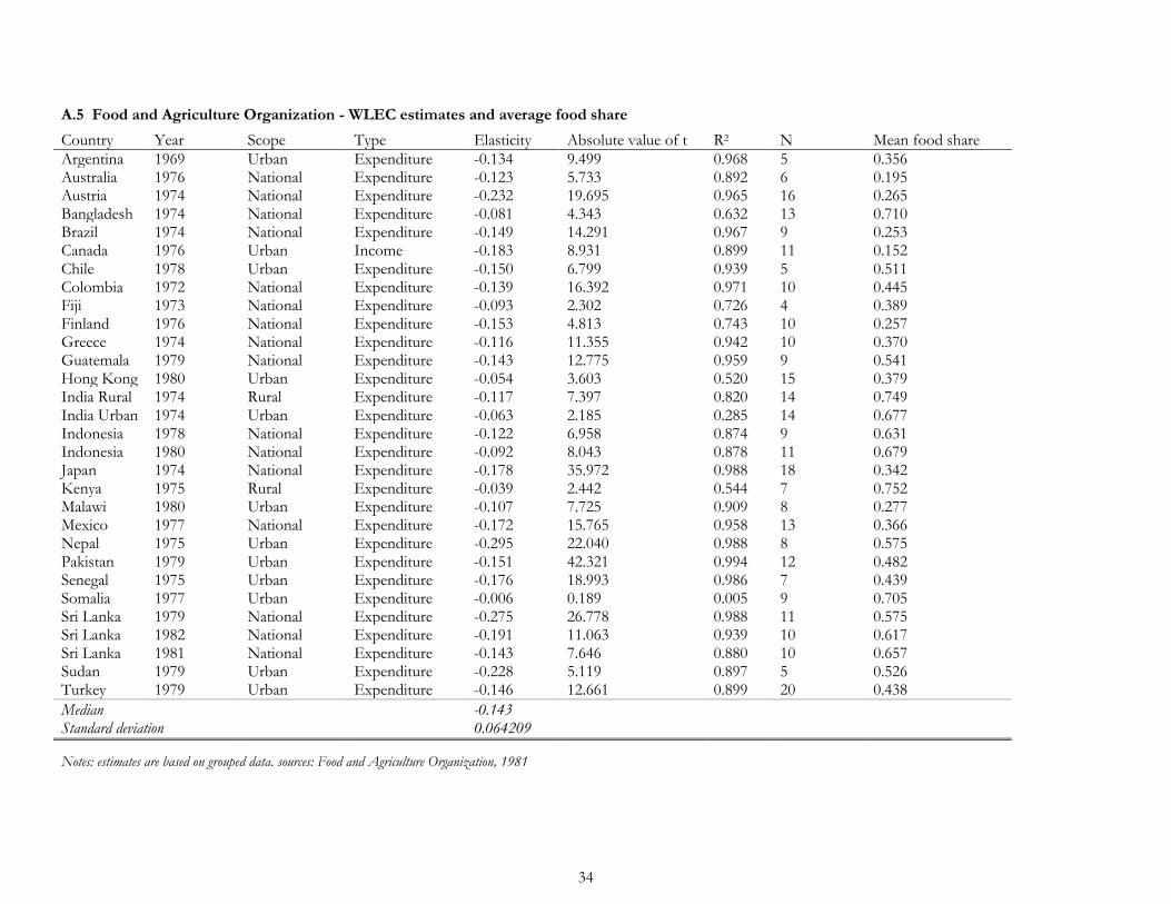
34

A.5 Food and Agriculture Organization - WLEC estimates and average food share

Country Year Scope Type Elasticity Absolute value of t R2 N Mean food share

Argentina 1969 Urban Expenditure -0.134 9.499 0.968 5 0.356 Australia 1976 National Expenditure -0.123 5.733 0.892 6 0.195 Austria 1974 National Expenditure -0.232 19.695 0.965 16 0.265 Bangladesh 1974 National Expenditure -0.081 4.343 0.632 13 0.710 Brazil 1974 National Expenditure -0.149 14.291 0.967 9 0.253 Canada 1976 Urban Income -0.183 8.931 0.899 11 0.152 Chile 1978 Urban Expenditure -0.150 6.799 0.939 5 0.511 Colombia 1972 National Expenditure -0.139 16.392 0.971 10 0.445 Fiji 1973 National Expenditure -0.093 2.302 0.726 4 0.389 Finland 1976 National Expenditure -0.153 4.813 0.743 10 0.257 Greece 1974 National Expenditure -0.116 11.355 0.942 10 0.370 Guatemala 1979 National Expenditure -0.143 12.775 0.959 9 0.541 Hong Kong 1980 Urban Expenditure -0.054 3.603 0.520 15 0.379 India Rural 1974 Rural Expenditure -0.117 7.397 0.820 14 0.749 India Urban 1974 Urban Expenditure -0.063 2.185 0.285 14 0.677 Indonesia 1978 National Expenditure -0.122 6.958 0.874 9 0.631 Indonesia 1980 National Expenditure -0.092 8.043 0.878 11 0.679 Japan 1974 National Expenditure -0.178 35.972 0.988 18 0.342 Kenya 1975 Rural Expenditure -0.039 2.442 0.544 7 0.752 Malawi 1980 Urban Expenditure -0.107 7.725 0.909 8 0.277 Mexico 1977 National Expenditure -0.172 15.765 0.958 13 0.366 Nepal 1975 Urban Expenditure -0.295 22.040 0.988 8 0.575 Pakistan 1979 Urban Expenditure -0.151 42.321 0.994 12 0.482 Senegal 1975 Urban Expenditure -0.176 18.993 0.986 7 0.439 Somalia 1977 Urban Expenditure -0.006 0.189 0.005 9 0.705 Sri Lanka 1979 National Expenditure -0.275 26.778 0.988 11 0.575 Sri Lanka 1982 National Expenditure -0.191 11.063 0.939 10 0.617 Sri Lanka 1981 National Expenditure -0.143 7.646 0.880 10 0.657 Sudan 1979 Urban Expenditure -0.228 5.119 0.897 5 0.526 Turkey 1979 Urban Expenditure -0.146 12.661 0.899 20 0.438

Median

-0.143 Standard deviation 0.064209

Notes: estimates are based on grouped data. sources: Food and Agriculture Organization, 1981

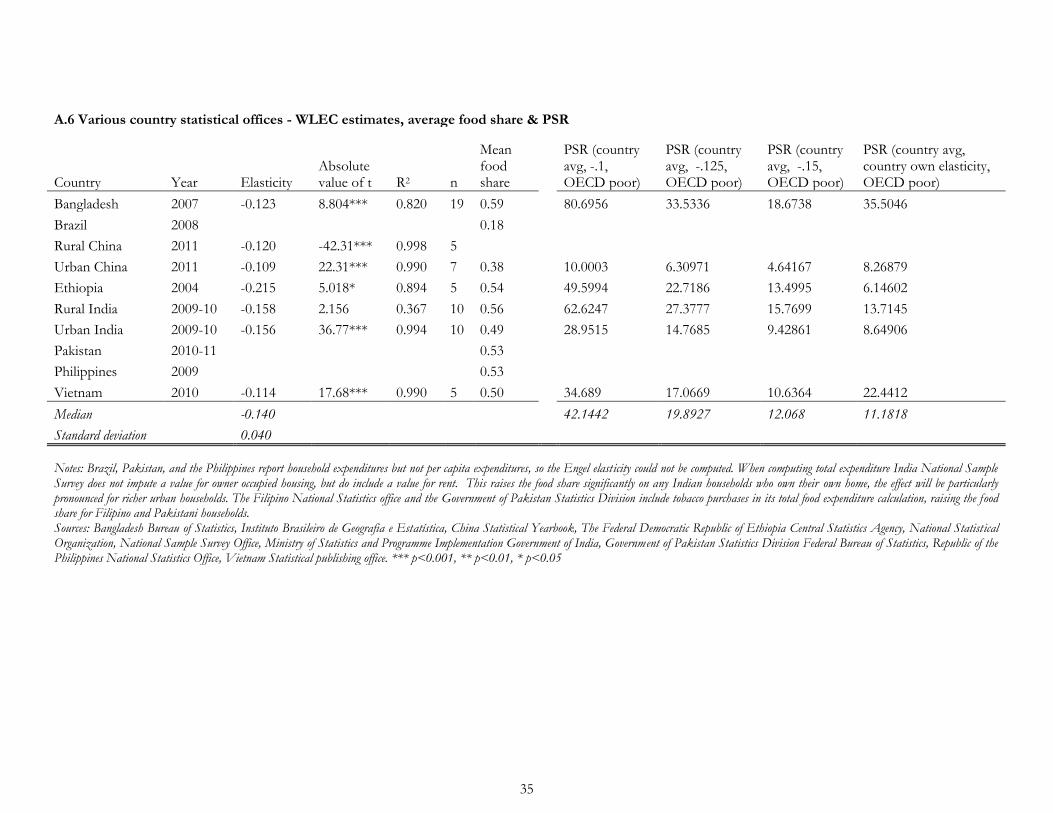
35

A.6 Various country statistical offices - WLEC estimates, average food share & PSR

Country Year Elasticity Absolute value of t R2 n

Mean food share

PSR (country avg, -.1, OECD poor)

PSR (country avg, -.125, OECD poor)

PSR (country avg, -.15, OECD poor)

PSR (country avg, country own elasticity, OECD poor)

Bangladesh 2007 -0.123 8.804*** 0.820 19 0.59

80.6956 33.5336 18.6738 35.5046

Brazil 2008

0.18 Rural China 2011 -0.120 -42.31*** 0.998 5

Urban China 2011 -0.109 22.31*** 0.990 7 0.38

10.0003 6.30971 4.64167 8.26879

Ethiopia 2004 -0.215 5.018* 0.894 5 0.54

49.5994 22.7186 13.4995 6.14602

Rural India 2009-10 -0.158 2.156 0.367 10 0.56

62.6247 27.3777 15.7699 13.7145

Urban India 2009-10 -0.156 36.77*** 0.994 10 0.49

28.9515 14.7685 9.42861 8.64906

Pakistan 2010-11

0.53 Philippines 2009

0.53

Vietnam 2010 -0.114 17.68*** 0.990 5 0.50

34.689 17.0669 10.6364 22.4412

Median -0.140

42.1442 19.8927 12.068 11.1818

Standard deviation 0.040

Notes: Brazil, Pakistan, and the Philippines report household expenditures but not per capita expenditures, so the Engel elasticity could not be computed. When computing total expenditure India National Sample Survey does not impute a value for owner occupied housing, but do include a value for rent. This raises the food share significantly on any Indian households who own their own home, the effect will be particularly pronounced for richer urban households. The Filipino National Statistics office and the Government of Pakistan Statistics Division include tobacco purchases in its total food expenditure calculation, raising the food share for Filipino and Pakistani households. Sources: Bangladesh Bureau of Statistics, Instituto Brasileiro de Geografia e Estatística, China Statistical Yearbook, The Federal Democratic Republic of Ethiopia Central Statistics Agency, National Statistical Organization, National Sample Survey Office, Ministry of Statistics and Programme Implementation Government of India, Government of Pakistan Statistics Division Federal Bureau of Statistics, Republic of the Philippines National Statistics Office, Vietnam Statistical publishing office. *** p<0.001, ** p<0.01, * p<0.05

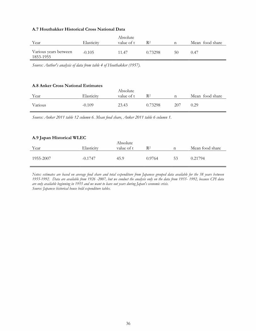
36

A.7 Houthakker Historical Cross National Data

Year Elasticity Absolute value of t R2 n Mean food share

Various years between 1853-1955

-0.105 11.47 0.73298 50 0.47

Source: Author's analysis of data from table 4 of Houthakker (1957).

A.8 Anker Cross National Estimates

Year Elasticity Absolute value of t R2 n Mean food share

Various -0.109 23.43 0.73298 207 0.29

Source: Anker 2011 table 12 column 6. Mean food share, Anker 2011 table 6 column 1.

A.9 Japan Historical WLEC

Year Elasticity

Absolute value of t R2 n Mean food share

1955-2007 -0.1747 45.9 0.9764 53 0.21794

Notes: estimates are based on average food share and total expenditure from Japanese grouped data available for the 38 years between 1955-1992. Data are available from 1926 -2007, but we conduct the analysis only on the data from 1955- 1992, because CPI data are only available beginning in 1955 and we want to leave out years during Japan's economic crisis. Source: Japanese historical house hold expenditure tables.

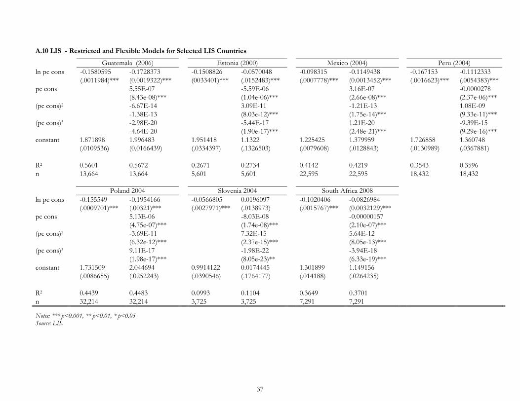
37

A.10 LIS - Restricted and Flexible Models for Selected LIS Countries

Guatemala (2006)

Estonia (2000)

Mexico (2004)

Peru (2004)

ln pc cons

-0.1580595 -0.1728373

-0.1508826 -0.0570048

-0.098315 -0.1149438

-0.167153 -0.1112333

(.0011984)*** (0.0019322)***

(0033401)*** (.0152483)***

(.0007778)*** (0.0013452)***

(.0016623)*** (.0054383)***

pc cons

5.55E-07

-5.59E-06

3.16E-07

-0.0000278

(8.43e-08)***

(1.04e-06)***

(2.66e-08)***

(2.37e-06)***

(pc cons)2

-6.67E-14

3.09E-11

-1.21E-13

1.08E-09

-1.38E-13

(8.03e-12)***

(1.75e-14)***

(9.33e-11)***

(pc cons)3

-2.98E-20

-5.44E-17

1.21E-20

-9.39E-15

-4.64E-20

(1.90e-17)***

(2.48e-21)***

(9.29e-16)***

constant

1.871898 1.996483

1.951418 1.1322

1.225425 1.379959

1.726858 1.360748

(.0109536) (0.0166439)

(.0334397) (.1326503)

(.0079608) (.0128843)

(.0130989) (.0367881)

R2

0.5601 0.5672

0.2671 0.2734

0.4142 0.4219

0.3543 0.3596

n

13,664 13,664

5,601 5,601

22,595 22,595

18,432 18,432

Poland 2004

Slovenia 2004

South Africa 2008

ln pc cons

-0.155549 -0.1954166

-0.0566805 0.0196097

-0.1020406 -0.0826984

(.0009701)*** (.00321)***

(.0027971)*** (.0138973)

(.0015767)*** (0.0032129)***

pc cons

5.13E-06

-8.03E-08

-0.00000157

(4.75e-07)***

(1.74e-08)***

(2.10e-07)***

(pc cons)2

-3.69E-11

7.32E-15

5.64E-12

(6.32e-12)***

(2.37e-15)***

(8.05e-13)***

(pc cons)3

9.11E-17

-1.98E-22

-3.94E-18

(1.98e-17)***

(8.05e-23)**

(6.33e-19)***

constant

1.731509 2.044694

0.9914122 0.0174445

1.301899 1.149156

(.0086655) (.0252243)

(.0390546) (.1764177)

(.014188) (.0264235)

R2

0.4439 0.4483

0.0993 0.1104

0.3649 0.3701

n

32,214 32,214

3,725 3,725

7,291 7,291

Notes: *** p<0.001, ** p<0.01, * p<0.05 Source: LIS.

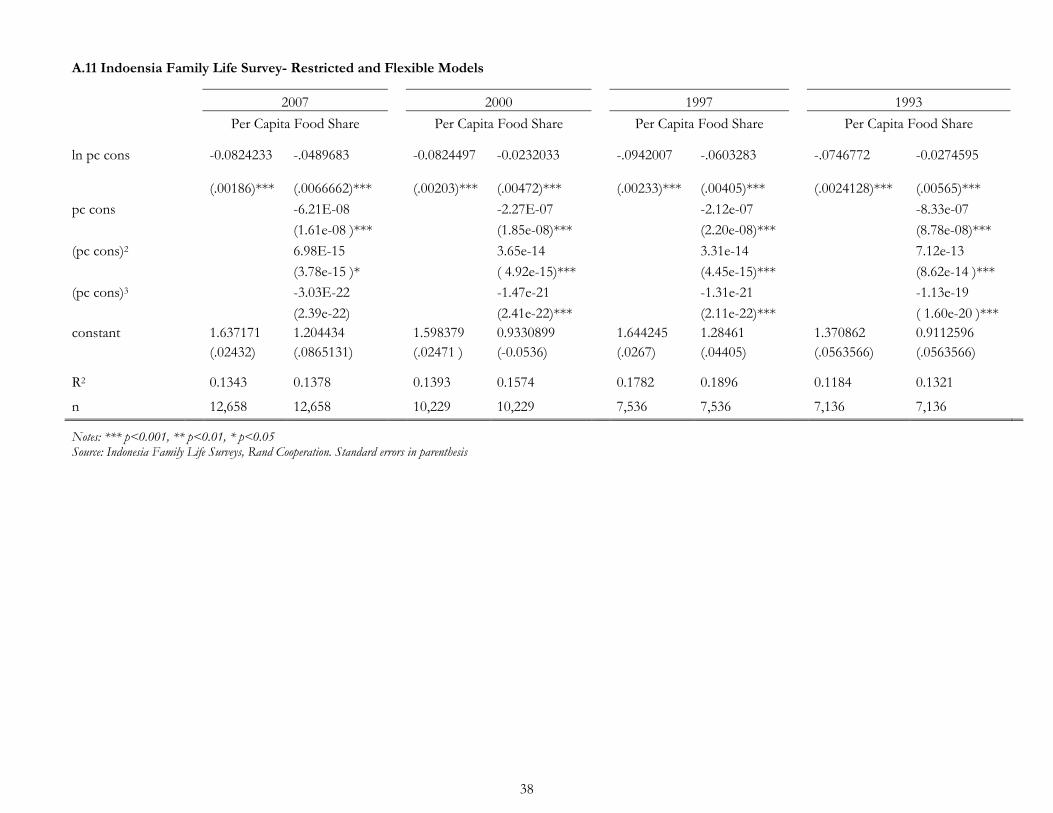
38

A.11 Indoensia Family Life Survey- Restricted and Flexible Models

2007

2000

1997

1993

Per Capita Food Share

Per Capita Food Share

Per Capita Food Share

Per Capita Food Share

ln pc cons

-0.0824233 -.0489683

-0.0824497 -0.0232033

-.0942007 -.0603283

-.0746772 -0.0274595

(.00186)*** (.0066662)***

(.00203)*** (.00472)***

(.00233)*** (.00405)***

(.0024128)*** (.00565)***

pc cons

-6.21E-08

-2.27E-07

-2.12e-07

-8.33e-07

(1.61e-08 )***

(1.85e-08)***

(2.20e-08)***

(8.78e-08)***

(pc cons)2

6.98E-15

3.65e-14

3.31e-14

7.12e-13

(3.78e-15 )*

( 4.92e-15)***

(4.45e-15)***

(8.62e-14 )***

(pc cons)3

-3.03E-22

-1.47e-21

-1.31e-21

-1.13e-19

(2.39e-22)

(2.41e-22)***

(2.11e-22)***

( 1.60e-20 )***

constant

1.637171 1.204434

1.598379 0.9330899

1.644245 1.28461

1.370862 0.9112596

(.02432) (.0865131)

(.02471 ) (-0.0536)

(.0267) (.04405)

(.0563566) (.0563566)

R2

0.1343 0.1378

0.1393 0.1574

0.1782 0.1896

0.1184 0.1321

n

12,658 12,658

10,229 10,229

7,536 7,536

7,136 7,136

Notes: *** p<0.001, ** p<0.01, * p<0.05 Source: Indonesia Family Life Surveys, Rand Cooperation. Standard errors in parenthesis

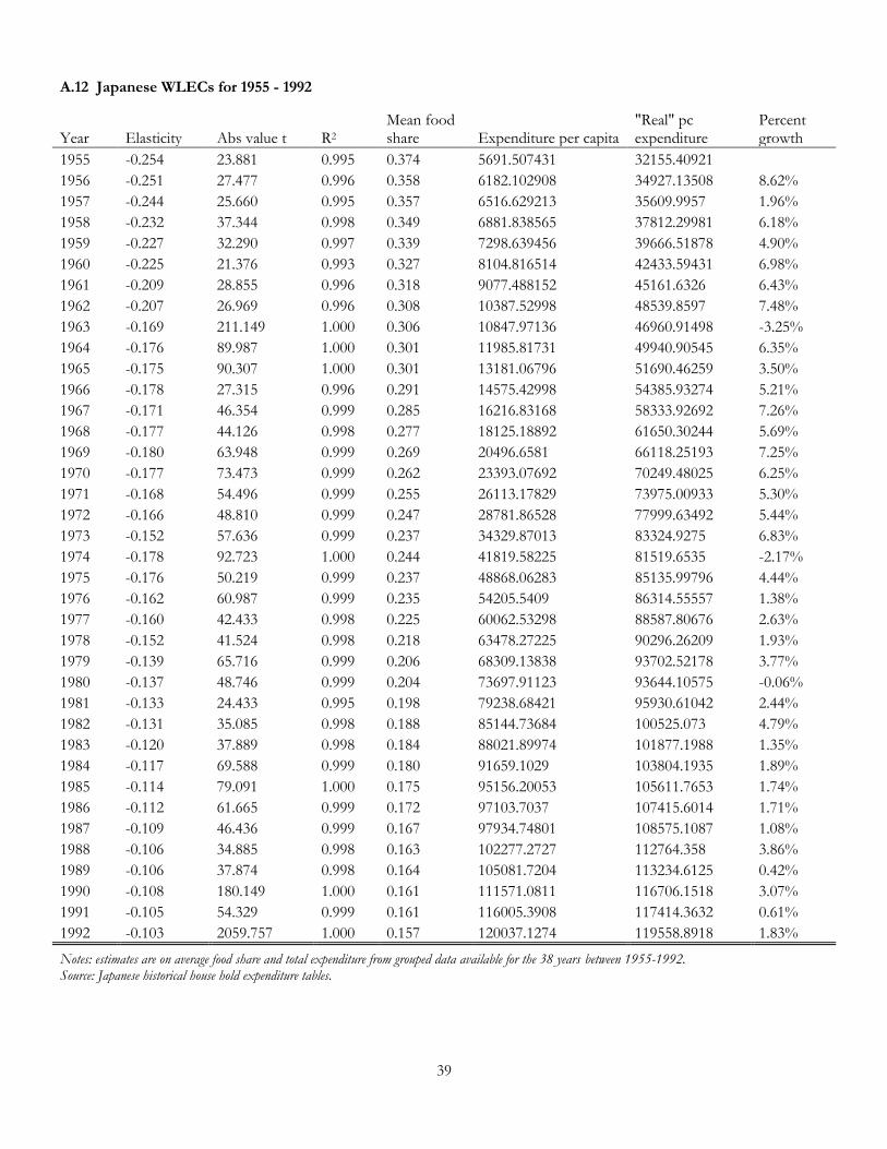
39

A.12 Japanese WLECs for 1955 - 1992

Year Elasticity Abs value t R2 Mean food share Expenditure per capita

"Real" pc expenditure

Percent growth

1955 -0.254 23.881 0.995 0.374 5691.507431 32155.40921 1956 -0.251 27.477 0.996 0.358 6182.102908 34927.13508 8.62%

1957 -0.244 25.660 0.995 0.357 6516.629213 35609.9957 1.96%

1958 -0.232 37.344 0.998 0.349 6881.838565 37812.29981 6.18%

1959 -0.227 32.290 0.997 0.339 7298.639456 39666.51878 4.90%

1960 -0.225 21.376 0.993 0.327 8104.816514 42433.59431 6.98%

1961 -0.209 28.855 0.996 0.318 9077.488152 45161.6326 6.43%

1962 -0.207 26.969 0.996 0.308 10387.52998 48539.8597 7.48%

1963 -0.169 211.149 1.000 0.306 10847.97136 46960.91498 -3.25%

1964 -0.176 89.987 1.000 0.301 11985.81731 49940.90545 6.35%

1965 -0.175 90.307 1.000 0.301 13181.06796 51690.46259 3.50%

1966 -0.178 27.315 0.996 0.291 14575.42998 54385.93274 5.21%

1967 -0.171 46.354 0.999 0.285 16216.83168 58333.92692 7.26%

1968 -0.177 44.126 0.998 0.277 18125.18892 61650.30244 5.69%

1969 -0.180 63.948 0.999 0.269 20496.6581 66118.25193 7.25%

1970 -0.177 73.473 0.999 0.262 23393.07692 70249.48025 6.25%

1971 -0.168 54.496 0.999 0.255 26113.17829 73975.00933 5.30%

1972 -0.166 48.810 0.999 0.247 28781.86528 77999.63492 5.44%

1973 -0.152 57.636 0.999 0.237 34329.87013 83324.9275 6.83%

1974 -0.178 92.723 1.000 0.244 41819.58225 81519.6535 -2.17%

1975 -0.176 50.219 0.999 0.237 48868.06283 85135.99796 4.44%

1976 -0.162 60.987 0.999 0.235 54205.5409 86314.55557 1.38%

1977 -0.160 42.433 0.998 0.225 60062.53298 88587.80676 2.63%

1978 -0.152 41.524 0.998 0.218 63478.27225 90296.26209 1.93%

1979 -0.139 65.716 0.999 0.206 68309.13838 93702.52178 3.77%

1980 -0.137 48.746 0.999 0.204 73697.91123 93644.10575 -0.06%

1981 -0.133 24.433 0.995 0.198 79238.68421 95930.61042 2.44%

1982 -0.131 35.085 0.998 0.188 85144.73684 100525.073 4.79%

1983 -0.120 37.889 0.998 0.184 88021.89974 101877.1988 1.35%

1984 -0.117 69.588 0.999 0.180 91659.1029 103804.1935 1.89%

1985 -0.114 79.091 1.000 0.175 95156.20053 105611.7653 1.74%

1986 -0.112 61.665 0.999 0.172 97103.7037 107415.6014 1.71%

1987 -0.109 46.436 0.999 0.167 97934.74801 108575.1087 1.08%

1988 -0.106 34.885 0.998 0.163 102277.2727 112764.358 3.86%

1989 -0.106 37.874 0.998 0.164 105081.7204 113234.6125 0.42%

1990 -0.108 180.149 1.000 0.161 111571.0811 116706.1518 3.07%

1991 -0.105 54.329 0.999 0.161 116005.3908 117414.3632 0.61%

1992 -0.103 2059.757 1.000 0.157 120037.1274 119558.8918 1.83%

Notes: estimates are on average food share and total expenditure from grouped data available for the 38 years between 1955-1992. Source: Japanese historical house hold expenditure tables.

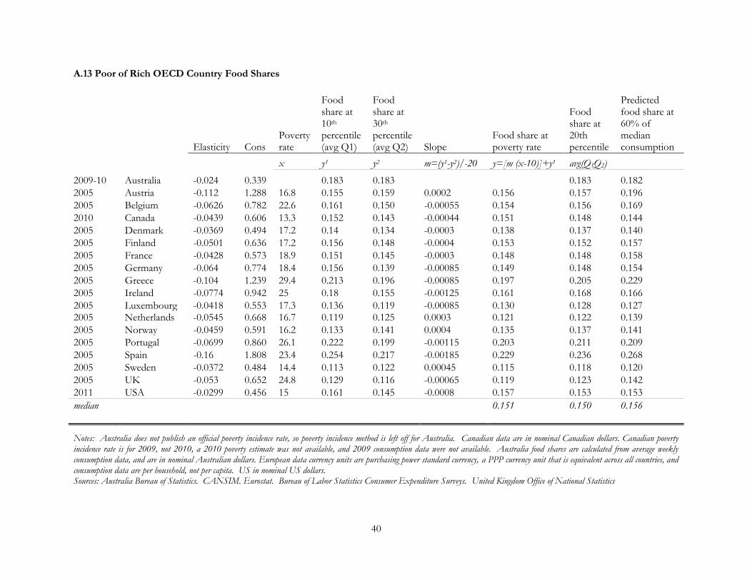
40

A.13 Poor of Rich OECD Country Food Shares

Elasticity Cons

Poverty rate

Food share at 10th percentile (avg Q1)

Food share at 30th percentile (avg Q2) Slope

Food share at poverty rate

Food share at 20th percentile

Predicted food share at 60% of median consumption

x y1 y2 m=(y1-y2)/-20 y=[m (x-10)]+y1 avg(Q1Q2)

2009-10 Australia -0.024 0.339

0.183 0.183

0.183 0.182

2005 Austria -0.112 1.288 16.8 0.155 0.159 0.0002 0.156 0.157 0.196

2005 Belgium -0.0626 0.782 22.6 0.161 0.150 -0.00055 0.154 0.156 0.169

2010 Canada -0.0439 0.606 13.3 0.152 0.143 -0.00044 0.151 0.148 0.144

2005 Denmark -0.0369 0.494 17.2 0.14 0.134 -0.0003 0.138 0.137 0.140

2005 Finland -0.0501 0.636 17.2 0.156 0.148 -0.0004 0.153 0.152 0.157

2005 France -0.0428 0.573 18.9 0.151 0.145 -0.0003 0.148 0.148 0.158

2005 Germany -0.064 0.774 18.4 0.156 0.139 -0.00085 0.149 0.148 0.154

2005 Greece -0.104 1.239 29.4 0.213 0.196 -0.00085 0.197 0.205 0.229

2005 Ireland -0.0774 0.942 25 0.18 0.155 -0.00125 0.161 0.168 0.166

2005 Luxembourg -0.0418 0.553 17.3 0.136 0.119 -0.00085 0.130 0.128 0.127 2005 Netherlands -0.0545 0.668 16.7 0.119 0.125 0.0003 0.121 0.122 0.139

2005 Norway -0.0459 0.591 16.2 0.133 0.141 0.0004 0.135 0.137 0.141

2005 Portugal -0.0699 0.860 26.1 0.222 0.199 -0.00115 0.203 0.211 0.209

2005 Spain -0.16 1.808 23.4 0.254 0.217 -0.00185 0.229 0.236 0.268

2005 Sweden -0.0372 0.484 14.4 0.113 0.122 0.00045 0.115 0.118 0.120

2005 UK -0.053 0.652 24.8 0.129 0.116 -0.00065 0.119 0.123 0.142

2011 USA -0.0299 0.456 15 0.161 0.145 -0.0008 0.157 0.153 0.153

median

0.151 0.150 0.156

Notes: Australia does not publish an official poverty incidence rate, so poverty incidence method is left off for Australia. Canadian data are in nominal Canadian dollars. Canadian poverty incidence rate is for 2009, not 2010, a 2010 poverty estimate was not available, and 2009 consumption data were not available. Australia food shares are calculated from average weekly consumption data, and are in nominal Australian dollars. European data currency units are purchasing power standard currency, a PPP currency unit that is equivalent across all countries, and consumption data are per household, not per capita. US in nominal US dollars. Sources: Australia Bureau of Statistics. CANSIM. Eurostat. Bureau of Labor Statistics Consumer Expenditure Surveys. United Kingdom Office of National Statistics

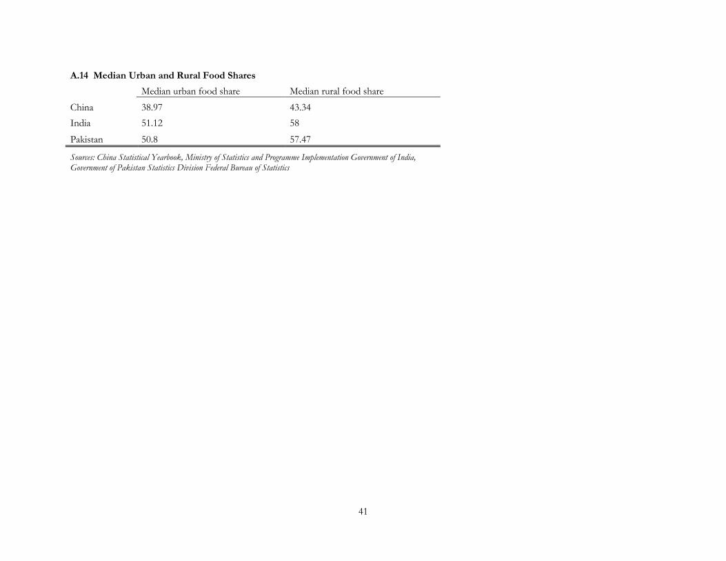
41

A.14 Median Urban and Rural Food Shares

Median urban food share Median rural food share

China 38.97 43.34

India 51.12 58

Pakistan 50.8 57.47

Sources: China Statistical Yearbook, Ministry of Statistics and Programme Implementation Government of India, Government of Pakistan Statistics Division Federal Bureau of Statistics