Estimating the Estimation of Accruals · 2019-05-14 · Estimating the Amount of Estimation in Accruals . Jason V. Chen . University of Michigan . Ross School of Business . [email protected]

Estimating the Amount of Estimation in Accruals

Jason V. Chen University of Michigan Ross School of Business

[email protected]

Feng Li University of Michigan Ross School of Business

[email protected]

February 15, 2013

Abstract

This paper examines the link between the amount of estimation needed during the accrual generating process and the persistence of the accruals portion of earnings. We measure the amount of estimation needed during the accrual generating process using the number of estimation-related linguistic cues in the notes to the financial statements and the critical accounting policies section of the management discussion and analysis. Consistent with the conjecture in Sloan [1996], we find that accruals that need more estimation are less predictive of future earnings. We also find that such accruals map less into the past, current, or future cash flows in the spirit of Dechow and Dichev [2002]. When we decompose the number of estimation linguistic cues into a component that is due to the existence of specific accruals accounts and a component that is due to the within-accounts variations, we find that our results are driven by both components. Lastly, we find mixed evidence as to whether the amount of estimation in accruals is systematically associated with the accrual anomaly. Overall, our results suggest that the estimation needed during the accrual generating process plays an important role in understanding the persistence of accruals.

We thank Matt DeAngelis, Ilia Dichev, Scott Richardson, Lakshmanan Shivakumar, Irem Tuna, and the workshop participants at University of Buffalo, Florida State University, London Business School, University of Michigan, Michigan State University, Purdue University, and Rice University for their comments. We gratefully acknowledge the support of the Ross School of Business and the financial support from the Paton Accounting Fellowship and the Harry Jones Endowment.

mailto:[email protected]

mailto:[email protected]

1

1. Introduction

We propose a new approach to measure the quality of accruals based on the amount of

estimation embedded in the accruals, calculated as the number of estimation-related linguistic

cues in the notes to the financial statements and the critical accounting policy (CAP) disclosures

in the management discussion and analysis. We empirically investigate the association between

this new measure of accruals quality and how predictive the accruals are of future earnings.

Our empirical tests are motivated by Sloan [1996] and Richardson et al. [2005], who

argue that the greater estimation needed in the accrual generating process explains why accruals

are less persistent than cash flows. Unlike cash flows, accruals incorporate estimates of future

cash flows, cash flow deferrals, depreciation and amortization, and fair value estimates. While

this argument is a well-accepted conjecture, few studies have explicitly examined how the

estimation involved in the accrual generating process relates to the persistence of accruals

(Dechow et al. [2010]). Rather, prior research has primarily examined how the different

components of accruals explain its persistence. For example, Dechow and Ge [2006] finds that

accruals exhibit lower persistence when they contain special items. Richardson et al. [2005]

examines the difference in persistence of working capital, non-current operating, and financial

asset accruals. We provide complementary evidence by linking accruals persistence directly to

the characteristics of the accruals generating process.

We focus on the footnotes to the financial statements and the critical accounting policies

disclosures in the management discussion and analysis to gauge the amount of estimation in

accruals since they contain detailed descriptions of the nature of the accruals and how they are

generated. Auditors and investors, however, have questioned their usefulness due to the large

amount of boilerplate and immaterial information in these disclosures (Radin [2007]). Our

empirical tests therefore can also be viewed as joint tests of the usefulness of the footnotes and

CAP disclosures for assessing accruals quality.

2

We start out by reading numerous footnotes and CAP disclosures in the financial

statements to find estimation-related linguistic cues. We find that in general, these linguistic cues

can be broken down into three linguistic relations: (1) An estimation action targets some object

(e.g. “we estimated receivables”), (2) An estimation object is the target of a use action (e.g. “we

used estimates”), (3) An estimation word is an adjective to an object (e.g. “estimated costs”). We

construct a dictionary of estimation-related words (see Appendix 2 for details) and count the

number of estimation-related linguistic cues for the three linguistic relations. We then use

statistical parsing techniques to automate the search for such linguistic cues in the footnotes and

CAP section of firms’ 10-K filings (Appendix 1).

Our first hypothesis is that accruals that require more estimation are less predictive of

future earnings. Consistent with this hypothesis, we find that accruals are significantly less

persistent when there is greater estimation conveyed in the company’s footnotes and CAP

disclosures. In contrast, we find that the amount of estimation conveyed in the company’s

footnotes and CAP is not informative of the persistence of cash flows. These findings support

Sloan’s conjecture that the amount of estimation needed in accruals partially explains their lower

persistence.

We also find that accruals that involve more estimation also have lower quality measured

in the sense of Dechow and Dichev [2002], i.e., these accruals map less into past, current, or

future cash flows. This is consistent with the hypothesis that more highly estimated accruals are

less precise, and therefore have greater errors, and provides further evidence that the estimation

needed during the accrual generating process drives the lower persistence.

A natural question arises whether the number of estimation cues simply captures the

types of accruals accounts.1 For instance, firms that have defined benefits pension plans are

likely to have more estimation cues in the footnote because pension calculations need to estimate

1 We thank Irem Tuna for this observation.

3

more parameters. We therefore decompose the number of estimation cues in the footnotes and

CAP disclosures into two components: a component that is due to the existence of specific

accruals accounts and a component that is due to the within-accounts variations. Specifically, we

identify 49 common accounting items (see footnote 6) and regress the number of estimation cues

on the item fixed effects. The predicted value from this model captures the number of estimation

cues due to the existence of different accruals accounts and the residual captures the within-

accounts variations. We find that the persistence of accruals and the quality of accruals are

driven by both components of the estimation cues.

Lastly, we examine the accrual anomaly as a function of the estimation cues in the

footnotes and CAP disclosures. We find mixed evidence as to whether the market reacts as if it

does not incorporate the amount of estimation in accruals into its valuation of the firm in a timely

manner. Specifically, we find some evidence that the accrual anomaly documented in prior

studies (Sloan [1996], Xie [2001], Mashruwala et al. [2006]) is more significant when more

estimation is needed during the accrual generating process. 2 This is consistent with the

hypothesis that the market more greatly overvalues (undervalues) highly estimated positive

(negative) accruals in the short term. However, the robustness tests of our findings using the

Carhart four-factor Alpha model provide mixed results.

We conduct a battery of robustness checks for our empirical results. First, we build

pseudo word counts by randomly selecting a dictionary of words that have similar aggregate

frequencies as our estimation cue words in the 10-K samples. The bootstrapping simulation

results show that the probability of finding the results documented in the paper using the pseudo

dictionary is low. Second, we extract the non-critical accounting policies part of the management

discussion and analysis in 10-Ks and count the number of estimation-related linguistic cues in

these disclosures. We find that the number of estimation-related linguistic cues in the non-CAP

2 Our study uses one-year abnormal returns which begin 5 days after the 10-K filing.

4

part of MD&As is not associated with accruals or earnings quality. This suggests that our

measure of the amount of estimation in accruals does not simply capture generic business

uncertainty. Lastly, we control for numerous other textual disclosure characteristics of the

financial statements documented in prior studies, including the Fog index (Li [2008]) and the

competition measures (Li, Lundholm, and Minnis [2012]), and our results are robust to these

controls.

We make several contributions to the literature. First, this study incorporates the amount

of estimation needed during the accrual generating process as reflected in a firm’s notes to the

financial statements and critical accounting policies disclosures into our understanding of the

persistence of accruals. Many prior studies have ignored this important source of information

about accruals when examining the persistence of accruals.3

Second, our findings strengthen Sloan’s argument that the estimation involved in accruals

explains the difference in the persistence of the cash portion of earnings and the accruals portion

of earnings. Some prior studies argue that the difference in the persistence of accruals and cash

flows documented by Sloan is driven by omitted fundamental differences such as growth. Our

findings suggest that estimation does explain the lower persistence of accruals.

Finally, this study contributes to the textual analysis accounting literature by using

grammatical relationships to extract meaning from qualitative financial information. These

relationships provide structure to the qualitative information and allow us to better infer meaning

from the text. Additionally, this study adds to a growing field of textual analysis studies which

suggest that using qualitative accounting information, in conjunction with quantitative

accounting information, helps to provide a richer understanding of firms and their accounting

process (Li [2011]).

3 Richardson et al. [2005] is an exception in that they test the association between accruals estimation and persistence by examining the properties of the different components of accruals.

5

The remainder of the paper proceeds as follows. Section 2 provides a discussion of prior

literature and motivation for our hypotheses. In Section 3 we discuss how the sample of 10-K

footnotes and CAP disclosures and financial information is prepared. In Section 4 we present the

research design and main results. Section 5 concludes the paper.

2. Prior Literature and Hypotheses

Sloan [1996] finds that the accruals portion of earnings is less predictive of future

earnings than the cash portion earnings (i.e. accruals are less persistent than cash flows). He

argues that the difference between the persistence of accruals and cash flows is due to the greater

estimation needed when deriving accruals, as accruals incorporate estimates of future cash flows,

depreciation and allocations, deferrals, and valuations. Richardson et al. [2005] expands the

hypothesis in Sloan [1996] and formally models accruals estimation as an error-in-variables

problem. Their model assumes that if accruals can be measured without error, there is no need to

correct for accrual errors in future periods. However, actual recorded accruals are measured with

error since managerial estimation is needed during the accrual generating process. This error

reduces the association between accruals and future earnings.

To test the hypothesis, prior studies have examined how the specific components that

comprise accruals affect how well accruals predict future earnings. For instance, Dechow and Ge

[2006] examines the persistence of low accruals when the firm has special items. Consistent with

their hypothesis, they find that accruals are less persistent when the firm has special items.

Richardson et al. [2005] disaggregates accruals into financing accruals, working capital accruals,

and non-current operating accruals. They posit that the accruals in each of the three categories

have different degrees of estimation. Financial accruals require less estimation than working

capital or non-current operating accruals because their terms are typically contractually defined.

Therefore estimates of future cash flows are well defined and require a lower degree of

6

estimation. On the other hand, estimates of future cash flows, valuations, and other estimates are

needed when recording working capital and non-current operating accruals. The greater

estimation in these accruals implies that these accruals are less likely to be realized in the cash

flows and therefore will be less informative of future earnings. Consistent with their hypothesis,

they find that financing accruals are more persistent than working capital and non-current

operating accruals.

In this paper, we argue that while on average accruals need more estimation than cash

flows, not all accruals are created equal. Due to differences in business fundamentals, accounting

policies, and earnings management incentives, accruals reported by different companies have

different levels of estimations and therefore different quality. Even if two companies have the

same total dollar amount of accruals, the amount of estimation in the accruals of these two

companies may be vastly different. For example, one company’s total accruals may contain a

large amount of estimated fair value accruals while another may contain a large amount of

financial accruals involving less estimation.

We fill the gap in the literature by explicitly measuring and examining the implications of

the cross-sectional differences in the amount of estimation in accruals on accruals persistence.

Accordingly, our first hypothesis follows the conjectures of Sloan [1996] and Richardson et al.

[2005] and is as follows:

Prediction 1: Accruals that involve more estimation are less persistent.

Dechow and Dichev [2002] finds that firms that exhibit a lower mapping of accruals into

past, current, and future cash flows also exhibit lower earnings persistence. They posit that if

accruals map less into these cash flows then accrual errors must be greater (i.e. the accruals are

recorded with low precision). Thus, accruals will be less predictive of future earnings.

7

We argue that if there is greater estimation in accruals then these accruals are likely to be

recorded with lower precision (i.e. accruals map less into realized cash flows). If managers make

a large number of estimations when recording accruals then the range of possible errors in the

recorded accruals is greater. When accruals have greater error, they are less realized as cash in

prior, current, or subsequent periods. Following this reasoning, greater estimation during the

accrual generating process will be associated with a lower mapping of cash flows into the

accruals portion of earnings.

Prediction 2: Accruals that involve more estimation map less into the firm’s past, current, or

future cash flows.

Prior studies have found that the lower persistence of accruals is not quickly incorporated

by investors in their valuations (Sloan [1996], Hanlon [2005], Richardson et al. [2005]). One

explanation for this finding is that investors fixate on total earnings thereby disregarding the

affect of the lower persistence of accruals on how predictive current earnings are of future

earnings (Sloan [1996], Kraft et al. [2006]). Accordingly, Sloan [1996] finds that the future

abnormal returns are negatively associated with the magnitude of firms’ accruals.

If investors fixate on total earnings and ignore the difference between accruals and cash

flows, then they may not fully incorporate the information in the amount of estimation in

accruals in the footnotes or CAP disclosures in a timely manner. This reasoning suggests that the

amount of estimation in accruals could exacerbate the accrual anomaly, i.e., accruals that need

more estimation are more likely to be mispriced and negatively associated with future stock

returns.

On the other hand, investors may quickly incorporate the amount of estimation in

accruals into their valuation of the firm since this information is readily available in the firm’s

8

10-K filings. More specifically, information provided in a firm’s footnote disclosures has been

shown to be incorporated by both investors and analysts (De Franco et al. [2011]). If the amount

of estimation involved in the accruals portion of earnings can be found in the notes to the

financial statements or CAP disclosures then investors may become informed of the lower

persistence of these earnings upon the filing of the 10-K. If so, then the estimation information

found in the footnotes or CAP disclosures will not be associated with the future long term

abnormal returns of the firm. This leads to our third prediction, stated in the null hypothesis

format:

Prediction 3: The market reacts as if it does not incorporate the amount of estimation in

accruals in their valuation of the firm in a timely manner.

3. Data Preparation 3.1 Extracting the Footnotes to the Financial Statements

We download all 10-K documents filed with the SEC for fiscal years between 1995 and

2010 from the SEC EDGAR Website.4 We then extract the notes to the financial statements and

the critical accounting policies disclosures in the management discussion and analysis section

from each of the 10-K filings using Perl. The extracted footnotes and CAP disclosures are

stripped of all HTML tags and tables. To mitigate any data issues related to extracting the notes

to the financial statements from each 10-K filing we truncate our sample of notes to the financial

statements and critical accounting policies by the total number of words at the 1% and 99%

level. We also eliminate any filings which are not explicitly identified as either a “10-K” or “10-

K405” in the filing’s header.

3.2 Measuring Accruals Estimation

4 Companies began filing using EDGAR beginning in 1994-1995.

9

Our textual analysis approach is used to capture the amount of estimation needed when

the accruals are recognized. We focus on the notes to the financial statements section and the

critical accounting policies section of the 10-K because they provide information specific to the

accounting process. The notes to the financial statements provide a wealth of information not

found in other sections of the 10-K filing (Merkeley [2011], Riedl and Srinivasan [2010]). More

importantly, this section provides comprehensive information pertaining to the estimations made

and the assumptions needed by management during the accrual generating process.

In May 2002, the Securities and Exchange Commission (SEC) begin to require firms to

include critical accounting policy (CAP) disclosures in their 10-K filings. In particular, the SEC

requires managers to provide a discussion of those accounting policies that involve highly

uncertain assumptions for which differing estimates would have a material influence on the

firm’s financial statements (Billings [2011]). Levine and Smith [2011] show that CAP

disclosures influence investors’ valuation decisions. For our purpose, the disadvantage of the

CAP disclosures is that it only covers the latter part of our sample period (i.e., post-2002 years).

We read numerous notes to the financial statements and critical accounting policies

disclosures to identify linguistic cues commonly used to denote that some estimation was

needed. The first linguistic cue is when an estimation action targets some object. For example,

the phrase “we estimated receivables” contains the estimation action “estimated” which targets

the object “receivables”. This cue denotes that receivables were estimated. Another linguistic cue

is when a “use action” targets an estimate object. An example of this is the phrase “we used

estimates” where the action “used” targets the object “estimates”. Lastly, the use of an estimate

adjective to modify some object also conveys that something was an estimate. An example of

this is “estimated costs”; here the object “costs” is being modified by the adjective “estimated”

thereby conveying that the costs are estimates.

10

We automate the search for these linguistic cues by first parsing each of the sentences in

our sample using the Stanford open source statistical parser (Marneffe et al. [2006]). The parse

of each sentence identifies its noun modifiers, direct object modifiers, adjective modifier, etc.

(i.e. its grammatical relationships). Deconstructing sentences in this manner not only provides us

with a map of the qualitative information but, more importantly, allows us to utilize the

grammatical relationships between the words in the each sentence. Using the grammatical

relationships allows us to more correctly identify linguistic cues that convey that some

estimation is needed by management (Klein and Manning [2003], see Appendix 1).

Next, we construct fours dictionaries to help us extract meaning from the sentence parses.

The first dictionary contains Estimation Actions. Words in the Estimation Actions dictionary

convey that an estimation action was performed – this dictionary includes words such as

“Estimate,” “Anticipate,” and “Approximate.” The second dictionary is of Estimation Objects

(Nouns). This dictionary contains estimation related objects and contains words such as “Belief,”

“Estimates,” and “Approximations.” The dictionary of Estimation Objects is used in conjunction

with a word from our Use Words dictionary, our third dictionary. This dictionary includes words

that denote that management use or need some object and includes words such as “Make,”

“Use,” and “Include.” Our fourth and final dictionary is Estimation Adjectives and contains

estimation words that are used to modify some object - these words include “Likely,”

“Estimated,” and “Anticipated”.

Finally, using our sentence parses and dictionaries we examine each sentence in our

sample of footnotes and CAP disclosures for the linguistic cues that we identified as conveying

that estimation is needed or used by management (see Appendix 2). 5 The number of these

5 We look for direct objects, nominal subjects, noun compound modifiers, adjectival modifiers, and quantifier phrase modifiers which convey that an estimation was made or used.

11

linguistic cues is used as our measure of the amount of estimation needed by management during

the accrual generating process.

3.2.1 Measuring Between-Accounts Estimations and Within-Accounts Estimations

We also decompose the number of estimation cues into a component that is due to the

existence of specific types of accruals accounts (“Between-Accounts Estimations” or BAE) and a

component that is due to within-account variations (“Within-Account Estimations” or WAE).

For instance, a firm could have more estimation cues simply because it has defined benefits

pension plans, which tend to involve more estimations than other accruals. On the other hand, it

is also possible that there are different levels of estimations for the same types of accounts or

transactions across companies. For example, the calculation of uncollectible receivables of one

company may need to estimate more parameters compared with those for another company.

We measure BAE and WAE by calculating the expected amount of estimation needed

given the specific items in the company’s notes to the financial statements and CAP disclosures.

Specifically, we extract all footnote headers from our sample of 10-K filings and sort them based

on their frequency. Starting with the most frequent footnote headers, we categorize

approximately one thousand unique footnote headers by hand and categorize them into 49 unique

footnote items.6 7 Using this list of unique footnote headers we then find which items appear in

each company’s notes to the financial statements. We then regress the number of estimation cues

on the account item fixed effects by industry and year:

6 The list of footnote headers are: Taxes, Accounting Policies, Commitments, Contingencies, Affiliates, Stock, Long-term Debt, Subsequent Events, PP&E, Inventory, Pension and Retirement, Mergers and Acquisitions, Financial Instruments, Earnings Per Share, Segment Information, Leases, Financial Data, Discontinued Operations, Investments, Stock Options, Payables, Cash, Intangibles, Stock Compensation, Business, Cash Flows, Other Assets, Receivables, Credit Arrangements, Regulatory, Derivatives, Going Concern, Credit Risk, Fair Value, Comprehensive Income, Significant Customers, Accounting Changes, Restructuring, Allowance, Parent Company, Restatement, Shareholder Rights, Loan, Dividends, Real Estate, Other Expenses, Joint Ventures, Supplemental Information, and Reinsurance. 7 The 1,000 hand categorized footnote headers directly account for approximately 70% of all footnote headers from our sample. This hand categorized sample was use to seed our Perl script which searched for footnote headers.

12

𝐸𝑠𝑡𝑖𝑚𝑎𝑡𝑖𝑜𝑛𝑓,𝑡 = 𝛽0 + Σ𝛽𝑗𝐹𝑜𝑜𝑡𝑛𝑜𝑡𝑒_𝑖𝑡𝑒𝑚𝑗,𝑓,𝑡 + 𝜖𝑓,𝑡 (1)

where 𝐸𝑠𝑡𝑖𝑚𝑎𝑡𝑖𝑜𝑛𝑓,𝑡 is the number of estimation-related linguistic cues in firm f’s notes to the

financial statement and CAP disclosures in year t. 𝐹𝑜𝑜𝑡𝑛𝑜𝑡𝑒_𝑖𝑡𝑒𝑚𝑗,𝑓,𝑡 is an indicator which

equals 1 if the company’s notes to the financial statements contain the specific footnote item j.

The predicted (residual) value from this model captures BAE (WAE), or the number of

estimation cues explained by the existence of different accruals accounts (the number of

estimation cues due to the within-accounts variations). Appendix (3) presents the top 10 and

bottom 10 account items in terms of the amount of estimation as indicated by the 𝛽 coefficients

in equation (1). Among the commonly seen transactions, the recording of “fair value,”

“intangibles,” “derivatives,” “restructuring,” “discontinued operations,” and “contingencies” has

the most amount of estimation-related linguistic cues; “PP&E,” “long-term debt,” “inventory,”

and “taxes” have the least amount of estimation-related linguistic cues.

We examine whether BAE and WAE have different implications for accruals persistence

and quality. Ex ante, we posit that both BAE and WAE explain the lower persistence of accruals

in comparison to cash flows.

3.3 Sample Preparation

We merge the estimation count data with annual financial information from the Wharton

Research Data Services (WRDS) Compustat database and equity market information from the

Center for Research in Security Prices (CRSP). For a handful of the firms in our sample were

unable to find corresponding financial data or market information. The main reason for many of

these stemmed from not being able to find an appropriate GVKEY for the CIK specified in the

header of the 10-K filing. We then eliminate financial institutions from our sample due to the

13

potential idiosyncratic nature of their accruals and disclosures.8 This leaves us with a sample size

of 64,411 firm year observations.

Future long window abnormal returns of the firm are calculated as the compounded

returns of the firm minus the compounded returns of the market over the same window.

Specifically, we calculated one-year compounded returns beginning five days after the filing of

the 10-K. We also calculated one-year value weighted compounded market returns beginning

five days after the 10-K filing for each of the firms in our sample. Compounded abnormal returns

for each firm are the calculated by subtracting the one-year value weighed compounded market

returns from the one-year compounded returns of the firm.

3.3.1 Summary Statistics

Table 1 presents the average estimation-related linguistic cues and the average total

number of words found in the notes to the financial statements and CAP disclosures. Consistent

with prior studies, we find that the average length of the footnotes and CAP disclosures has

steadily increased over time (Li [2008]). On average, the length of the notes to the financial

statements and CAP disclosures has doubled in size over our sample period going from an

average of 5,194 words for the fiscal period 1995 to 14,695 words in 2010. This finding is also

consistent with prior studies and anecdotal evidence that suggest that firms’ financial disclosures

have been increasing in complexity (Radin [2007]). We also find that the amount of estimation-

related linguistic cues has increased monotonically during our sample period. Specifically, the

number of linguistic cues that convey estimation increased from an average 33 in the fiscal

period 1995 to an average of 130 in 2010.

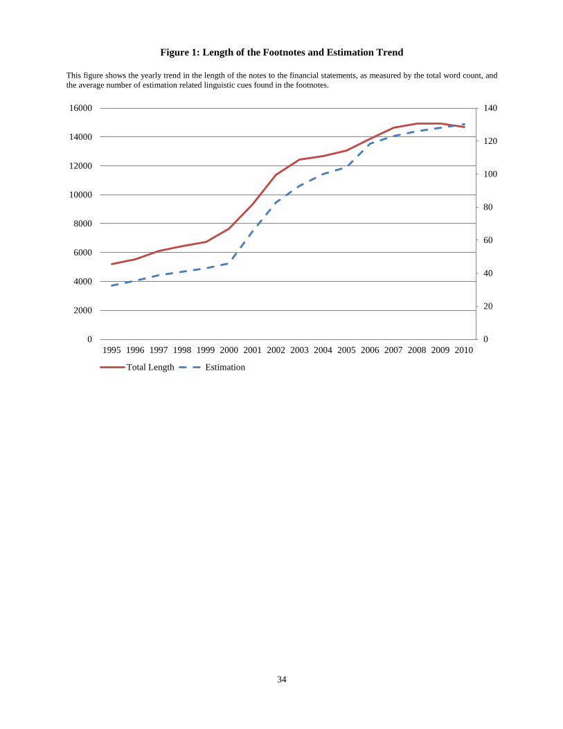
Figure 1 plots the trend of estimation and of the length of the footnotes and CAP

disclosures (as measured by the total number of words in the footnotes and CAP disclosures) and

reiterates our description of the trend in both footnotes length and estimation. Overall, the length

8 Financial firms are identified as those firms having SIC codes between 6000 and 6999.

14

of the footnotes and CAP disclosures has been growing over the years in our sample. Moreover,

the estimation count has been growing as well. There appears to be a slight leveling off in the

growth of the footnotes in the later periods of our sample. To control for the time-trend in the

length in footnotes and CAP disclosures, we include year fixed effects and the total number of

words in the empirical tests.

Table 2 shows the average estimation and the average number of words in the notes to the

financial statements and CAP disclosures by industry. Industry appears to play an important role

in the amount of estimation. Agricultural production crops, automotive repair, building materials,

social services, and construction contractors are the 5 industries with the least amount of

estimation having an average of approximately 36 estimation linguistic cues in their footnotes.

On the other hand. the industries of coal mining, communications, paper and allied products,

and oil and gas constitute the 5 industries with the most amount of accruals estimation and have

an average of 102 estimation related linguistic cues in the footnotes.

4. Research Design and Results

4.1 Determinants of Estimation

In this section, we perform cross-sectional tests to examine the associations between

certain firm characteristics and the amount of estimation needed in its accruals. This exercise

serves two purposes. First, it provides some intuitive validation to our measure. Second and

perhaps more importantly, these firm characteristics could be potential control variables when

we examine the implications of our estimation measure for accruals quality.

We examine the following set of variables identified in prior studies (Dechow and

Dichev [2002], Francis et al. [2005]) as potential determinants of the amount of estimation in

accruals:

15

Size

Larger firms typically have more operational complexity than smaller firms. This

suggests that greater estimation is needed to convey the activities of the firm through accruals.

However, everything else equal, the transactions of larger firms can have diversification effects,

which may make the estimation of accruals more precise. For instance, firms with a diverse set

of receivables may be able to estimate the bad debt ratio more precisely to the extent that the

different sources of receivables offer some diversifications. Therefore, ex ante we do not have a

clear prediction on the association between firm size and the amount of estimation in accruals.

Negative Earnings

Accounting conservatism suggests that accountants tend to require a higher degree of

verification to recognize good news as gains than to recognize bad news as losses (Basu [1997]).

This suggests that positive earnings need a greater degree of certainty to be recognized while

negative earnings may be recognized with less precision (i.e., more estimation). We therefore

hypothesize that firms with negative earnings are more likely to have more estimation needed in

their accruals.

Operating Cycle

Longer operating cycles imply a longer horizon for accruals to be mapped into realized

cash flows. Therefore more estimates (and more imprecise estimates) may be needed by

management when calculating and recognizing accruals. We predict a positive association

between the operating cycle of a firm and the amount of estimation in its accruals.

Standard Deviation of Cash flows and Standard Deviation of Sales

Firms with more volatile business environment are more likely to have accruals that need

more estimation. We use two variables, the standard deviation of cash flows and the standard

deviation of sales (both scaled by the book value of assets), to test for this positive prediction.

16

We use both variables because sales could be affected by the amount of accruals booked (e.g.,

receivables) and cash flows are not subject to this problem.

We perform our cross-sectional test using the following tobit model left censored at 0 to

examine the relationship between the determinants of the amount of estimation in accruals:

𝐸𝑠𝑡𝑖𝑚𝑎𝑡𝑖𝑜𝑛𝑓,𝑡 = 𝛽0 + 𝛽1Size𝑓,𝑡 + 𝛽2𝑂𝑝𝑒𝑟𝑎𝑡𝑖𝑛𝑔𝐶𝑦𝑐𝑙𝑒𝑓,𝑡

+𝛽3𝑠𝑡𝑑𝑒𝑣(𝑆𝑎𝑙𝑒𝑠)𝑓,𝑡 + 𝛽4𝑠𝑡𝑑𝑒𝑣(𝐶𝑎𝑠ℎ 𝐹𝑙𝑜𝑤𝑠)𝑓,𝑡+𝛽5𝑁𝐸𝐺𝐸𝐴𝑅𝑁𝑓,𝑡 + 𝜖𝑓,𝑡,

(2)

where 𝐸𝑠𝑡𝑖𝑚𝑎𝑡𝑖𝑜𝑛𝑓,𝑡 is defined earlier. S𝑖𝑧𝑒𝑓,𝑡 is the log of the market value of the firm’s equity.

𝑂𝑝𝑒𝑟𝑎𝑡𝑖𝑛𝑔_𝐶𝑦𝑐𝑙𝑒𝑓,𝑡 is the length of the operating cycle of the firm calculated as log ( 𝑖𝑛𝑣𝑡𝑐𝑜𝑔𝑠

∗

360 + 𝑟𝑒𝑐𝑡𝑠𝑎𝑙𝑒𝑠

∗ 360), where invt is the average inventory balance and cogs is the cost of goods

sold. 𝑠𝑡𝑑𝑒𝑣(𝑆𝑎𝑙𝑒𝑠)𝑓,𝑡 is the standard deviation of the firms sales (scaled by the book value of

assets) over the past five years. 𝑠𝑡𝑑𝑒𝑣(𝐶𝑎𝑠ℎ 𝐹𝑙𝑜𝑤𝑠) 𝑓,𝑡 is the standard deviation of the firms

cash flows (scaled by the book value of assets) over the past five years. 𝑁𝐸𝐺𝐸𝐴𝑅𝑁𝑓,𝑡 is the

number of years that the firm had negative earnings over the past 5 years. The empirical results

based on a simple Ordinary Least Squared regression are similar to those based on the tobit

model.

4.1.1 Determinants of Estimation Findings

Table 5 presents the results for the determinants of estimation in accruals. Consistent with

our expectations, the standard deviation of sales and the length of the operating cycle are

positively associated with Estimation, and the number of the past five years in which the firm has

17

negative earnings is negatively correlated with Estimation. The positive and significant

coefficient on size suggests that larger firms tend to report accruals that need more estimation.

One of the proxies for the volatility of business environment, the standard deviation of

cash flows, is statistically significant but the coefficient loads is in the opposite direction of our

prediction. One explanation for this surprising result is that in an uncertain environment,

managers simply may not book the imprecisely estimated accruals in the financial statements

since they are very uncertain of future cash flows due to the high volatility.

4.2 Estimation and the Persistence of Accruals

To test our first prediction (P1), we examine how the amount of estimation in accruals is

related to the persistence of earnings and the persistence of accruals relative to cash flows. We

follow prior literature (Sloan [1996], Li [2008]) and measure the persistence of earnings

(accruals and cash flows) by regressing the following year’s earnings on the current year’s

earnings (accruals and cash flows). All variables are scaled by the average book value of assets

for the period. Fundamentally, this regression measures how predictive current earnings

(accruals and cash flows) are of future earnings. If the estimated coefficient on current earnings

(accruals and cash flows) is high then we would conclude that current earnings (accruals and

cash flows) are highly persistent since they are highly associated with future earnings and vice

versa when the estimated coefficient on earnings in the regression is low.

First, we examine the marginal effect of the amount of estimation in accruals on the

persistence of total earnings. We include the interaction between the current year’s earnings and

the amount of estimation to measure the impact of estimation on the persistence of earnings. For

a given level of earnings, how much more (or less) persistent are they for a given level of

estimation. If our hypothesis is correct then we should find a negative coefficient on this

interaction term.

18

𝐸𝑎𝑟𝑛𝑖𝑛𝑔𝑠𝑓,𝑡+1 = 𝛽0 + 𝛽1𝐸𝑎𝑟𝑛𝑖𝑛𝑔𝑠𝑓,𝑡 + 𝛽2𝐸𝑠𝑡𝑖𝑚𝑎𝑡𝑖𝑜𝑛𝑓,𝑡

+𝛽3𝐸𝑎𝑟𝑛𝑖𝑛𝑔𝑠𝑓 ∗ 𝐸𝑠𝑡𝑖𝑚𝑎𝑡𝑖𝑜𝑛𝑓,𝑡 + 𝛴𝛽𝑖𝐶𝑜𝑛𝑡𝑟𝑜𝑙𝑠𝑓,𝑡 + Σ𝛽𝑗𝐸𝑎𝑟𝑛𝑖𝑛𝑔𝑠𝑓,𝑡 ∗ 𝐶𝑜𝑛𝑡𝑟𝑜𝑙𝑠𝑓,𝑡

+ 𝐴𝑢𝑑𝑖𝑡𝑜𝑟𝐹𝐸𝑓 + 𝑌𝑒𝑎𝑟𝐹𝐸𝑡 + IndustryFEf + 𝜖𝑓,𝑡

(3)

where 𝐸𝑠𝑡𝑖𝑚𝑎𝑡𝑖𝑜𝑛𝑓,𝑡 is defined earlier and 𝐸𝑎𝑟𝑛𝑖𝑛𝑔𝑠 is income before extraordinary items. The

controls include size, operating cycle, standard deviation of sales, standard deviation of operating

cash flows, the number of years over the past 5 years in which the firm had negative earnings,

and the total length of the footnotes. The first five control variables are the determinants of the

amount of estimation in accruals as examined in Table 5. They are included to make sure that

Estimation does not simply capture these common firm characteristics. We include the total

length of the footnotes to rule of the possibility that Estimation does not simply proxy for the

length of the document, since longer footnotes and CAP disclosures are more likely to contain

more estimation related linguistic cues. We also include interactions between all control

variables and earnings and auditor, year, and industry fixed effects.9 All continuous variables are

scaled by average total assets.

Next, we disaggregate earnings into cash flows and accruals and interact each component

with our measure of estimation. We follow the recommendations made in Hribar and Collins

[2002] and calculate accruals using the statement of cash flows. If greater estimation lowers the

association between the current year’s accruals the following year’s earnings then the interaction

between estimation and the accruals portion of earnings will be negative. Ideally, if the number

of linguistic cues that convey estimation in the footnotes and CAP disclosures does not capture

9 We include the interaction between the control variables and earnings since we want to control for the marginal impact of the control variable on the persistence of earnings in addition to the control variables impact on future performance.

19

the precision of the cash portion of earnings the interaction between cash flows and estimation

should be statistically insignificant.10

𝐸𝑎𝑟𝑛𝑖𝑛𝑔𝑠𝑓,𝑡+1 = 𝛽0 + 𝛽1𝐶𝑎𝑠ℎ𝑓,𝑡 + 𝛽2𝐴𝑐𝑐𝑟𝑢𝑎𝑙𝑠𝑓,𝑡 + 𝛽3𝐸𝑠𝑡𝑖𝑚𝑎𝑡𝑖𝑜𝑛𝑓,𝑡

+ 𝛽4𝐶𝑎𝑠ℎ𝑓,𝑡 ∗ 𝐸𝑠𝑡𝑖𝑚𝑎𝑡𝑖𝑜𝑛𝑓,𝑡 + 𝛽5𝐴𝑐𝑐𝑟𝑢𝑎𝑙𝑠𝑓,𝑡 ∗ 𝐸𝑠𝑡𝑖𝑚𝑎𝑡𝑖𝑜𝑛𝑓,𝑡 + 𝛴𝛽𝑖𝐶𝑜𝑛𝑡𝑟𝑜𝑙𝑠𝑓,𝑡

+ Σ𝛽𝑖𝐴𝑐𝑐𝑟𝑢𝑎𝑙𝑠𝑓,𝑡 ∗ 𝐶𝑜𝑛𝑡𝑟𝑜𝑙𝑠𝑓,𝑡 + Σ𝛽𝑖𝐶𝑎𝑠ℎ𝑓,𝑡 ∗ 𝐶𝑜𝑛𝑡𝑟𝑜𝑙𝑠𝑓,𝑡

+ 𝐴𝑢𝑑𝑖𝑡𝑜𝑟𝐹𝐸𝑓 + 𝑌𝑒𝑎𝑟𝐹𝐸𝑡 + IndustryFEf + 𝜖𝑓,𝑡

(4)

where 𝐸𝑠𝑡𝑖𝑚𝑎𝑡𝑖𝑜𝑛𝑓,𝑡 , 𝐸𝑎𝑟𝑛𝑖𝑛𝑔𝑠 , and the control variables are as defined in equation (3);

𝐶𝑎𝑠ℎ𝑓,𝑡 is the portion of total earnings due to operating cash flows and A𝑐𝑐𝑟𝑢𝑎𝑙𝑠𝑓,𝑡is the portion

of total earnings due to accruals. Like other continuous variables in the regression, both Cash

and Accruals are scaled by the average book value of assets.

In addition to controlling for the common firm characteristics when examining the

accruals and cash flows persistence test in equation (4), we also include three accruals quality

measures documented in prior studies. Specifically, we include the absolute value of the

magnitude of accruals (Sloan [1996]), the standard deviation of the Dechow and Dichev [2002]

residual, and special items (Dechow and Ge [2006]) in our tests of accruals persistence. By

examining the incremental power of Estimation in explaining accruals persistence, we can test

whether the footnotes and CAP disclosures can provide additional information about accruals

quality that is not reflected in other commonly used accruals quality measures.

4.2.1 Estimation and the Persistence of Accruals Findings

Table 6 presents the results for the regression of next year’s earnings on current year’s

earnings, estimation, the interaction between estimation and the current year’s earnings, and our

10 The measure of estimation may also capture business uncertainty about the firm. If so then the coefficient on the interaction between cash flows and estimation will also be negative and statistically significant.

20

controls (4). The coefficient on the interaction between estimation and earnings in the current

year is negative and statistically significant at 1%; this result suggests that earnings that need

more estimation are less persistent than those that required less estimation. The economic

significance of the effect of estimation on the persistence of earnings when going from the 25th

percentile of Estimation to the 75th is approximately -0.063 (-0.0009 * (106 – 36)); this translates

into a percentage difference of approximately 10% to 15% when compared to the baseline

persistence of accruals (Dechow et al. [2006]). Overall, these findings suggest that the amount of

estimation needed during the accrual generating process is associated with an economically

significant decrease in the persistence of total earnings.

The 3rd Column of Table 6 shows the interactions between BAE and WAE and earnings.

Both interaction terms are statistically significant at the 1% level. The magnitude of the

difference in the persistence of earnings when going from the 25th percentile of BAE to the 75th

percentile of BAE is -0.072 (-0.0010 * (111 – 39)). The economic magnitude when going from

the 25th to the 75th percentile of WAE is -0.0168 (-0.0008 * (9 + 12)).

As discussed before, accruals are one component of total earnings and the measure of the

amount of estimation should only pertain to the accruals portion of earnings and not the cash

flows portion. Table 7 shows the results when we interact each component of earnings separately

with our measure of estimation.11 As predicted the interaction between accruals and estimation is

negative and statistically significant; this result is consistent with our prediction that accruals that

need more estimation exhibit lower persistence. The difference in the persistence of accruals

between the 25th percentile of Estimation and the 75th percentile is approximately -0.07 (-0.0010

* (106 - 36)). Next, the results show that the coefficient on the interaction between cash flows

11 In untabluated results, consistent with prior research we find that the persistence of accruals is less than that of cash earning and that the magnitudes of the coefficients are similar to those found in prior research.

21

and the amount of estimation is statistically insignificant. This finding suggests that our measure

of estimation captures some characteristic of accruals but not cash flows.

The 5th Column of Table 7 shows the interaction between the amount of BAE and WAE

and both accruals and cash flows. Our findings suggest that the lower persistence of accruals in

comparison to cash flows is driven by both components of estimation. The interaction between

the amount of BAE and earnings and the interaction between WAE and earnings are both

statistically significant. The difference in the persistence of earnings when going from the 25th

percentile to the 75th percentile of BAE is approximately -0.0792 (-0.0011 * (111 – 39)) while

the difference in the persistence of accruals is -0.0168 (-0.0008 * (9 + 12)). An F-test of the

coefficients on the interaction between BAE and accruals and WAE and accruals yields a p-value

of 0.6457 thereby suggesting that the coefficients are not statistically different.

Table 8 presents the accruals and cash flows persistence test in equation (4) by further

including three accruals quality measures documented in prior studies: the absolute value of the

magnitude of accruals, the standard deviation of the Dechow and Dichev [2002] residual, and

special items. We estimate the Dechow and Dichev model as modified by McNichols [2002] by

industry and year and use the standard deviation of the residual from the model over the past 5

years for each firm as a measure of accruals quality (see equation (5) in the next section for more

details).

Table 8 Column 4 of Panel A shows that consistent with the findings in prior studies, all

three measures are statistically significant at the 1% level and negatively associated with the

persistence of accruals. Moreover, the standard deviation of the Dechow and Dichev residual and

Special Items are associated with a lower persistence of cash flows; this result suggests that these

measures pickup uncertainty about the cash flows of the firm as well.

Importantly, even after including these alternate measures of estimation we see that our

measure of estimation is still associated with a lower persistence of accruals at the 1% level of

22

significance. However, the economic significant of our measure has decreased to -0.049, a

reduction of approximately 30% from the economic significance found in Table 7. Even so, these

findings suggest that our measure is informative about some aspect of accruals persistence not

found in these other measures.

Panel B shows the results when we disaggregate estimation into BAE and WAE. BAE

remains statistically significant at the 10% level and is still negatively associated with the

persistence of accruals. On the other hand, the within-accounts portion of estimation is no longer

statistically significant but the sign of the coefficient is still negative.

4.3 Estimation and the Mapping of Accruals into Cash Flows

Prediction 2 (P2) suggests that when greater estimation is needed during the accrual

generating process accruals are less likely to be realized as cash. We use the measure of how

well accruals map into cash flows developed by Dechow and Dichev [2002] (hereafter DD) to

capture this effect. This model captures accruals quality by estimating how well working capital

accruals map to into realized operating cash flows. The model is based on the premise that

accruals are a way to shift the recognition of cash flows.12 If the realized cash flows of the firm

map well into the accruals of the firm then the firm’s accruals are deemed to be of high quality.

On the other hand, low-quality accruals consist of estimation errors will be reversed without any

cash flow implications. DD operationalize their theory by regressing current period working

capital accruals on prior period, current period, and next periods operating cash flows. The

standard deviation of the residual from this model is the measure of how well the firm’s accruals

map into cash flows.

12 This model does not distinguish between managed earnings or those which arise due to unintentional errors or management uncertainty.

23

The specification of the DD model is shown in equation (5). We include the change in

revenues and Property, Plant and Equipment (PPE) in the model as proposed in McNichols

[2002].

𝑇𝐶𝐴𝐶𝐶𝑓,𝑡 = β0 + 𝛽1𝐶𝐹𝑂𝑓,𝑡−1 + 𝛽2𝐶𝐹𝑂𝑓,𝑡 + 𝛽3𝐶𝐹𝑂𝑓,𝑡+1

+𝛽4Δ𝑅𝑒𝑣𝑓,𝑡 + 𝛽5𝑃𝑃𝐸𝑓,𝑡 + 𝜖𝑓,𝑡

(5)

where 𝐶𝐹𝑂 are the operating cash flows of the firm. 𝑇𝐶𝐴𝐶𝐶𝑓,𝑡 is the total working capital

accruals of firm. Δ𝑅𝑒𝑣𝑓,𝑡 is the change in sales from the prior year. 𝑃𝑃𝐸𝑓,𝑡 is the total property

plant and equipment for the current fiscal period. All continuous variables are scaled by average

total assets.

We estimate the model by industry and year and use STD(DD Residual), the standard

deviation of the residual from the model over the past 5 years for each firm, as our measure of

how well the accruals of the firm map into cash flows of the firm. We expect a positive

association between STD(DD Residual) and Estimation since accruals with more estimation

needed are likely to have lower quality and map less into cash flows.

4.3.1 Estimation and the Mapping of Accruals into Cash Flow Findings

Table 9 presents the results for how estimation affects how well accruals map into cash

flows (P2). Column 2 of Table 9 shows the regression of the determinants of accruals quality as

identified in Francis et al. [2005]. All of the determinants of accruals quality are statistically

significant and load in the same direction as found in prior studies (Francis et al. [2005], Dechow

and Dichev [2002]).

The 3rd Column of Table 9 includes our measure of estimation into the model and we find

that estimation is statistically significant at the 5% level and is positively associated with the

24

standard deviation of the Dechow and Dichev residual. This finding is consistent with our

hypothesis that the amount of estimation in accruals is associated with greater accrual errors and

therefore associated with a lower mapping of cash flows into accruals.

The 4th Column of Table 9 presents the results when we decompose estimation into BAE

and WAE. Once again we see that both components of estimation are statistically significant at

the 5% level and positively associated with a lower mapping of accruals into cash flows. An F-

test of the equality of the coefficients on BAE and WAE yields a p-value of 0.5693 therefore we

can’t reject the null that BAE and WAE have the same implications for accruals quality. This

result suggests that both components of estimation affect the mapping of accruals into cash flows

similarly. Overall our findings suggest that when there is a greater amount of estimation during

the accrual generating process there is a lower mapping of accruals into cash flows.

4.4 Estimation and Future Abnormal Returns

For our test of P3 we follow the research design of Sloan [1996] and Richardson et al.

[2005] to determine whether the market reacts as if it quickly incorporates the estimation

information found in the footnotes and CAP disclosures. Sloan [1996] regresses future abnormal

returns on total accruals and finds a negative association between the two. Therefore, positive

accruals are associated with negative future abnormal returns. On the other hand, negative

accruals are associated with positive future abnormal returns. These findings are consistent with

his hypothesis that the market over-values the persistence of accruals.

We make several small but important modifications to the research design for our study.

Since we are interested in the incremental effect of the amount of estimation on the persistence

of accruals we include the interaction between the amount of estimation and total accruals into

the model. The interaction term models the marginal effect of the amount of estimation on the

association between current accruals and future abnormal returns. If the interaction effect is

25

negative then this suggests that the market overvalues more highly estimated positive accruals

and vice versa for negative accruals.

Next, we make two small changes to the specification of the model to better coincide

with our research design. First, Sloan [1996] calculates future abnormal returns beginning four

months after the end of the firm’s fiscal period. In contrast, our abnormal returns accumulation

begins 5 days after firm files their 10-K form with the SEC. The information about the

estimation of accruals used in this study is found in the firm’s 10-K filing. Therefore, we need to

ensure that the estimation information found in the footnotes to the financial statements and CAP

disclosures is available to the market before we can assess whether the market incorporated the

information in a timely manner. Of course, some of the estimation information may have been

released prior to the filing of the 10-K but this would only bias results away from our prediction

since the market would have had more time to incorporate the information. Second, rather than

using a decile ranking of accruals we use the raw amount of accruals. One of the purposes of

Sloan [1996] is to show that a trading strategy could be implemented by purchasing stock in

firms with extreme low accruals and shorting those with extreme high accruals. The purpose of

this study isn’t to implement a trading strategy but rather the provide evidence that the markets

appear to not quickly incorporate the estimation information found in the footnotes. Therefore, to

preserve more of the information in accruals, we use the raw accruals amount rather than the

decile ranking of the amount of accruals.

𝐴𝑏𝑛𝑟𝑒𝑡𝑢𝑟𝑛𝑠𝑓,𝑡 = β0 + 𝛽1𝐴𝑐𝑐𝑟𝑢𝑎𝑙𝑠𝑓,𝑡 + 𝛽2𝐸𝑠𝑡𝑖𝑚𝑎𝑡𝑖𝑜𝑛𝑓,𝑡

+𝛽3𝐸𝑠𝑡𝑖𝑚𝑎𝑡𝑖𝑜𝑛𝑓,𝑡 ∗ 𝐴𝑐𝑐𝑟𝑢𝑎𝑙𝑠𝑓,𝑡 + 𝛽4𝑆𝑖𝑧𝑒𝑓,𝑡 + 𝛽5𝐵𝑇𝑀𝑓,𝑡

+𝛽6𝐸𝑇𝑃𝑓,𝑡 + 𝛽7𝐵𝑒𝑡𝑎𝑓,𝑡 + 𝜖𝑓,𝑡

(6)

26

where 𝐸𝑠𝑡𝑖𝑚𝑎𝑡𝑖𝑜𝑛𝑓,𝑡 is defined earlier. A𝑐𝑐𝑟𝑢𝑎𝑙𝑠𝑓,𝑡 is income before extraordinary items minus

operating cash flows. S𝑖𝑧𝑒𝑓,𝑡 is the log of the market value of the firms equity. 𝐵𝑇𝑀𝑓,𝑡 is the

book to market ratio of the firm. 𝐸𝑇𝑃𝑓,𝑡 is the firms earnings to price ratio. B𝑒𝑡𝑎𝑓,𝑡 is the market

beta of the firm for fiscal period t. 𝐴𝑏𝑛𝑟𝑒𝑡𝑢𝑟𝑛𝑠𝑓,𝑡 is one-year market-adjusted abnormal returns

beginning 5 days after the filings of the 10-K.

We also use the Fama-French Carhart four-factor model to further test the association

between accruals estimation and future abnormal returns. More specifically, we construct 25

portfolios each month based on the amount of accruals of the firm and the amount of estimation

conveyed in the notes to financial statements – 5 rankings of accrual x 5 rankings of estimation.

For each portfolio we then estimate the four-factor alpha using the following model.

𝑀𝑜𝑛𝑡ℎ𝑦𝐸𝑥𝑟𝑡 = 𝛽0 + 𝛽1𝑀𝑘𝑡𝐸𝑥𝑟𝑡 + 𝛽2𝐻𝑀𝐿𝑡 + 𝛽3𝑆𝑀𝐵𝑡 + 𝛽4𝑈𝑀𝐷𝑡 + 𝜖𝑡 (7)

where 𝑀𝑜𝑛𝑡ℎ𝑦𝐸𝑥𝑟𝑡 is the monthly excess return of the value or equal weighted portfolios.

𝑀𝑘𝑡𝐸𝑥𝑟𝑡 is the monthly return of the value-weighted index minus the risk free rate. 𝐻𝑀𝐿𝑡 is the

monthly premium of the book-to-market factor. 𝑆𝑀𝐵𝑡 is the monthly premium of the size factor;

𝑈𝑀𝐷𝑡 is the monthly premium on winners minus losers.13

4.4.1 Estimation and Returns Findings

The second columns of Table 10 present the baseline results shown in Sloan [1996]. For

our sample we find that accruals are negatively associated with the future abnormal returns of the

firm. Column 3 of Table 10 shows the results of our test of P3 - the association between future

long-term abnormal returns and the amount of estimation information found in the footnotes to

13 RF, HML, SMB, and UMD factors are from Ken French’s website.

27

the financial statements and CAP disclosures. The coefficient on the interaction between

estimation and total accruals is negative and statistically significant at the 1% level. Therefore,

accruals that require more estimation are more negatively associated with future long-term

abnormal returns. This is consistent with the hypothesis that investors are more likely to

overvalue firms with less persistent positive accruals and undervalue those with less persistent

negative accruals when the amount of estimation is larger. Column 4 presents the results of the

model when we decompose estimation into BAE and WAE. We find that the negative

association between abnormal returns and the interaction of accruals and estimation is primarily

driven by BAE.

Table 11 presents the results for our test of P3 using the Carhart four-factor model.

Overall we find mixed results as to whether the accrual anomaly is most concentrated in those

firms with the greatest amount of accruals estimation. Panel A of Table 11 presents the results

for the top and bottom most portfolios in terms of estimation and accruals. We construct hedged

returns by going long in those firms with the greatest accruals and short in those with the least

amount of accruals. When using equal weighted hedged returns we find evidence that accruals

are associated with future abnormal returns in our sample. However, we do not find any

association between the future abnormal returns of the firm and accruals when using value

weighted hedge returns.

We then examine whether the association between future abnormal returns and the

current years accruals are greater for those firms with the greatest amount of accruals estimation.

We do not find any evidence consistent with the hypothesis that the accrual anomaly is

exacerbated in those firms with greater estimation. This result is consistent with the hypothesis

that investors utilize the estimation information found in the notes to the financial statements and

CAP disclosures when valuing the firm.

28

Lastly, Panel B disaggregates estimation into BAE and WAE. We find no discernible

association between future abnormal returns and the amount of estimation and accruals when

using value-weighted returns. Using equal-weighted returns we find little difference between the

high and low estimation portfolios when using BAE. However, we do find some evidence that

those firms with the least WAE are associated with the future abnormal returns of the firm.

5. Robustness Tests

5.1 Placebo Tests Based on Bootstrapping

To address the question of whether the results using our linguistic cues approach are

“random” we conduct bootstrap tests of our main findings, Prediction 1 (P1) and Prediction 2

(P2). We begin this test by ranking all of the words in all of the notes to the financial statements

in our sample by their frequencies. Then, for each of the 40 words in our Estimation Actions,

Estimation Objects, and Estimation Adjectives dictionaries that appear at least once in a firm’s

notes to the financial statements we select the 5 words which lie above and the 5 words which lie

below that word in our frequency list.14 This process yields 10 unique dummy words for each

estimation words and a total of 400 unique placebo estimation words which we will refer to as

our placebo estimation words dictionary. This placebo dictionary contains words which have a

similar frequency of use as our main dictionaries but whose variation of use is likely different

from the dictionaries that we used in our study.

We begin our simulation by randomly selecting 1 word from the 10 dummy words

chosen for each estimation word to arrive at a list of 40 placebo estimation words and count the

number of times each of the placebo words is mentioned in a firms footnotes or CAP section;

14 The words anticipating, approximation, approximations, beliefs, believing, estimations, and expecting were never mentioned in a firms footnotes but were included in the original dictionaries for completeness.

29

this count is our placebo estimation count.15 We then estimate the models for the tests of (P1)

and (P2) using the placebo estimation count in place of our original count of the number of

estimation related linguistic cues. We use this simple word count approach instead of the

statistical parser due to computing constraints. This process of selecting random words and

retesting our hypotheses is repeated 1,000 times.

Table 12 presents our results for the joint tests of significance (insignificance).

Specifically, we are interested in what percentage of the bootstrapped tests yields a similar

pattern of results as those found using out estimation dictionaries. We see that only 3% of the

bootstrap placebo tests yield similar results to our main findings for the persistence of earnings

and the quality of accruals, (P1) and (P2) respectively. Specifically, only 3% of the bootstraps

yielded a negative and statistically significant result on the coefficient of earnings interacted with

the placebo estimation count (P1a), a negative and statistically significant results on the

interaction between accruals and the placebo estimation count and insignificant result on the

coefficient of the interaction between cash flows and the placebo estimation count (P1b), and a

positive and statically significant association between the placebo estimation count at the

standard deviation of the Dechow and Dichev residual (P2). This finding suggests that it is

unlikely that the results of study are purely random. Next, we see that only 6% of the

bootstrapped tests yield similar joint results for (P1a) and (P1b). Lastly, 11% of the bootstraps

yield similar joint results to our main findings for (P1b).

We also use the number of estimation-related linguistic cues in a firm’s non-critical

accounting policy part of the management discussion and analysis in its 10-K filing to replace

our Estimation variable in the empirical tests for P1 and P2. Such an estimation count is not

directly related to the accruals recognition, and is likely to capture the generic business

15 As an additional robustness check, we randomly select 40 words from the 400 placebo words instead of 1 word from the 10 placebo words chosen for each estimation word. This change in the selection process does not significantly affect the results of our simulation.

30

uncertainty only. Therefore, we do not expect to find similar empirical results using this variable.

In untabulated results, we find that indeed this variable is not statistically significantly associated

with earnings persistence, accruals persistence, or the Dechow-Dichev accruals quality.

5.2 Controlling for Other Textual Characteristics of 10-Ks

Prior studies have found that the persistence of earnings is lower for those firms whose

notes to the financial statements are more difficult to read (Li [2008]). It is possible that the

details about the accruals that require more estimation are more difficult to convey in writing.

Therefore, notes to the financial statements that are more difficult to read may actually convey

that greater estimation was needed during the accruals generating process. To address this issue

we calculate the Gunning-Fog index score for each of the notes to the financial statements in our

sample and include the calculated fog score (and its interaction with earnings, accruals, and cash

flows) in each of our main tests. In untabluated results we find that our results are not sensitive to

this specification.

Li, Lundholm, and Minnis [2012] show that the perceived competition intensity as

reflected in firms’ 10-K filings is associated with the mean-reverting speed of abnormal profit.

Untabulated results confirm that our results remain essentially the same if the competition

measure and its interactions with earnings, accruals, and cash flows are included as additional

control variables.

6. Conclusion

The primary focus of this study was to examine the association between the estimation

needed during the accrual generating process and the persistence of accruals. Sloan [1996] and

Richardson et al. [2005] suggest that the estimation needed when recording accruals reduces the

persistence of accruals. Their hypotheses are based on the idea that if accruals require a greater

31

degree of estimation they are more likely to be recorded with error (i.e. accruals are less precise).

If so, then accruals will be less predictive of future earnings. While this conjecture has been

generally accepted in the accounting literature few have explicitly examined the association

between the estimation involved during the accrual generating process and the persistence of

accruals.

This study provides evidence consistent with the conjecture that the estimation needed

during the accrual generating process plays a key role in the persistence of accruals. Specifically,

we find that when accruals have more estimation they are less predictive of future earnings. We

also find that accruals map less into the past, current, or future cash flows of the firm when they

require more estimation. Next, we find that both the between-accounts and within-accounts

portions of estimations drive our results. Lastly, we find mixed evidence as to whether the

markets do not quickly incorporate the estimation information found in firms’ footnotes into

their valuation of the firm.

In conclusion, the findings in this study provide insight into the accrual generating

processing of the managers. More importantly, the findings in our study suggest that

understanding the process which managers undergo when recording accruals plays an important

role in understanding the persistence and quality of accruals.

32

References Basu, S. 1997. The conservatism principle and the asymmetric timeliness of earnings. Journal of Accounting & Economics 24 (December): 3-37. Billings, M.B., 2011, Discussion of ‘Critical accounting policy disclosures’ by C. Levine and M. Smith, Journal of Accounting, Auditing and Finance. Dechow, P., I. Dichev, 2002, The Quality of Accruals and Earnings: The Role of Accrual Estimation Errors, The Accounting Review 77, 35-59. Dechow, P., W. Ge, 2006, The Persistence of Earnings and Cash Flow and the Roles of Special Items: Implications for the Accrual Anomaly, Review of Accounting Studies, 253-296. Dechow, P., W. Ge, C. Schrand, 2010, Understanding earnings quality: A review of the proxies, their determinants and their consequences. Journal of Accounting and Economics, 50(2-3), 344–401. Dechow, P. R. Sloan, A. Sweeney, 1995, Detecting Earnings Management, The Accounting Review 70, 193-225. De Franco, G., F. Wong, Y. Zhou, 2011, Accounting Adjustments and the Valuation of Financial Statement Note Information in 10-K Filings, The Accounting Review, Forthcoming. Francis, J., R. LaFond, P. Olsson, K. Schipper, 2005, The Market Pricing of Accruals Quality, Journal of Accounting and Economics 39, 295-327. Hanlon, M., 2005, The Persistence and Pricing of Earnings, Accruals, and Cash Flows When Firms Have Large Book-Tax Differences, The Accounting Review 80, 137-166. Hribar, P., D. Collins, 2002, Errors in Estimating Accruals: Implications for Empirical Research, Journal of Accounting Research 40. Jones, J., 1991, Earnings Management During Import Relief Investigations. Journal of Accounting Research 29, 193–228. Klein, D. and C. Manning, 2003, “Accurate Unlexicalized Parsing” Proceedings of the 41st Meeting of the Association for Computational Linguistics, 423-430. Kraft, A., A. Leone, C. Wasley, 2006, An Analysis of the Theories and Explanations Offered for the Mispricing of Accruals and Accrual Components. Journal of Accounting Research, 44(2), 297–339. Levine, C. B., and Michael J. S. 2011. “Critical Accounting Policy Disclosures.” Journal of Auditing, Accounting and Finance 26 (Winter): 39–75. Li, F., 2008, Annual Report Readability, Current Earnings, and Earnings Persistence, Journal of Accounting and Economics 45, 221-247.

33

Li, F., 2011, Textual Analysis of Corporate Disclosures: A Survey of the Literature, Journal of Accounting Literature, 29, 143-165. Li, F., R. Lundholm, M. Minnis, 2012, A Measure of Competition Based on 10-K Filings, Journal of Accounting Research. Marneffe, M., B. MacCartney, C. Manning, 2006, Generating Typed Dependency Parses from Phrase Structure Parses. LREC 2006. Merkley, K., 2010, More Than Numbers: R&D-related Disclosure and Firm Performance, Working Paper, Cornell University. Mashruwala, C., S. Rajgopal, & T. Shevlin, 2006, Why is the accrual anomaly not arbitraged away? The role of idiosyncratic risk and transaction costs. Journal of Accounting and Economics, 42(1-2), 3–33. McNichols, M., 2002, Discussion of The Quality of Accruals and Earnings: The Role of Accrual Estimation Errors, The Accounting Review 77, 61-69. Radin, A., 2007, Have We Created Financial Statement Disclosure Overload?, The CPA Journal. http://www.nysscpa.org/cpajournal/2007/1107/perspectives/p6.htm Richardson, S., R. Sloan, M. Soliman, I. Tuna, 2005, Accrual Reliability, Earnings Persistence and Stock Prices, Journal of Accounting and Economics 39, 437-485. Riedl, E., S. Srinivasan, 2010, Signaling Firm Performance Through Financial Statement Presentation: An Analysis Using Special Items, Contemporary Accounting Research 27, 289-332. Sloan, R. 1996, Do Stock Prices Fully Reflect Information in Accruals and Cash Flows About Future Earnings?, The Accounting Review 71, 289-315. United States Securities and Exchange Commission, SEC Form 10-K General Instructions, http://www.sec.gov/about/forms/form10-k.pdf. United States Securities and Exchange Commission, SEC Act of 1934, http://www.sec.gov/about/laws/sea34.pdf. White, H., 2010, An Accrual Balance Approach to Assessing Accrual Quality. Working Paper.

Xie, H., 2001, The Mispricing of Abnormal Accruals, (3), 357–373.

http://www.sec.gov/about/forms/form10-k.pdf

http://www.sec.gov/about/laws/sea34.pdf

34

Figure 1: Length of the Footnotes and Estimation Trend

This figure shows the yearly trend in the length of the notes to the financial statements, as measured by the total word count, and the average number of estimation related linguistic cues found in the footnotes.

0

20

40

60

80

100

120

140

0

2000

4000

6000

8000

10000

12000

14000

16000

1995 1996 1997 1998 1999 2000 2001 2002 2003 2004 2005 2006 2007 2008 2009 2010

Total Length Estimation

35

Table 1 : Estimation Trend

This table presents the average number of estimation related linguistic cues and the total number of words found in the notes to the financial statements and the critical accounting policies sections for our sample. Our sample spans from fiscal year 1995 to 2010.

Year Estimation Length N

1995 33 5194 2667

1996 35 5534 4686

1997 39 6101 4849

1998 41 6444 4717

1999 43 6744 4819

2000 46 7642 4671

2001 65 9331 4373

2002 83 11360 4144

2003 93 12419 3914

2004 100 12688 3850

2005 104 13054 3557

2006 118 13861 3566

2007 123 14612 3604

2008 126 14938 3839

2009 128 14924 3673

2010 130 14695 3482

Average 82 10596 4026

36

Table 2: Estimation by Industry This table shows average number of estimation related linguistic cues and the average number of words in the notes to the financial statements and critical accounting polices section by industry for fiscal periods between 1995-2010.

Industry Two Digit SIC Estimation Total Length N

Agricultural Production Crops 1 31 5651 16

Metal Mining 10 87 11642 380

Coal Mining 12 132 15852 55

Oil And Gas Extraction 13 89 11391 2445

Mining And Quarrying Of Nonmetallic Minerals, Except Fuels 14 52 6862 77

Building Construction General Contractors And Operative Builders 15 69 9872 423

Heavy Construction Other Than Building Construction Contractors 16 80 10006 154

Construction Special Trade Contractors 17 41 5955 98

Food And Kindred Products 20 69 9269 1504

Textile Mill Products 22 52 7368 308

Apparel And Other Finished Products Made From Fabrics 23 67 9384 682

Lumber And Wood Products, Except Furniture 24 65 7974 315

Furniture And Fixtures 25 63 7951 450

Paper And Allied Products 26 90 10311 660

Printing, Publishing, And Allied Industries 27 71 9035 894

Chemicals And Allied Products 28 82 11518 6255

Petroleum Refining And Related Industries 29 85 11132 410

Rubber And Miscellaneous Plastics Products 30 68 8895 838

Leather And Leather Products 31 48 7794 203

Stone, Clay, Glass, And Concrete Products 32 68 8425 401

Primary Metal Industries 33 74 9578 1024

Metal Products, Except Machinery And Transportation Equipment 34 68 8041 1068

Industrial And Commercial Machinery And Computer Equipment 35 77 9344 4304

Electronic And Other Electrical Equipment And Components 36 84 10051 5723

Transportation Equipment 37 84 9695 1458

Measuring, Analyzing, And Controlling Instruments 38 75 9429 4351

Miscellaneous Manufacturing Industries 39 66 8346 730

37

Table 2: Estimation by Industry (continued) This table shows average number of estimation related linguistic cues and the average number of words in the notes to the financial statements and critical accounting polices section by industry for fiscal periods between 1995-2010.

Industry Two Digit SIC Estimation Total Length N

Railroad Transportation 40 51 7905 49

Motor Freight Transportation And Warehousing 42 61 7519 540

Water Transportation 44 83 11461 265

Transportation By Air 45 84 10289 479

Transportation Services 47 74 10533 276

Communications 48 93 13085 2467

Electric, Gas, And Sanitary Services 49 108 14284 3279

Wholesale Trade-durable Goods 50 60 8521 1848

Wholesale Trade-non-durable Goods 51 69 10029 1037

Building Materials, Hardware, Garden Supply, And Mobile Home Dealers 52 35 5961 36

General Merchandise Stores 53 71 8465 427

Food Stores 54 67 8320 437

Automotive Dealers And Gasoline Service Stations 55 79 11313 344

Apparel And Accessory Stores 56 67 8839 752

Home Furniture, Furnishings, And Equipment Stores 57 47 6585 290

Eating And Drinking Places 58 67 8896 1235

Miscellaneous Retail 59 64 9419 1500

Hotels, Rooming Houses, Camps, And Other Lodging Places 70 61 8077 264

Personal Services 72 57 8632 143

Business Services 73 82 10794 8680

Automotive Repair, Services, And Parking 75 34 5022 21

Motion Pictures 78 78 11216 401

Amusement And Recreation Services 79 73 11030 856

Health Services 80 82 11110 1378

Educational Services 82 76 10012 291

Social Services 83 41 6949 65

Engineering, Accounting, Research, Management, And Related Services 87 78 10986 1526

Nonclassifiable Establishments 99 66 9805 299

38

Table 3: Summary Statistics

This table shows the summary statistics for the sample used in this study. Total Earnings is the firms income before extraordinary items scaled by average total assets. Accruals are total accruals scaled by average total assets. Operating Cash Flows are operating cash flows scaled by average total assets. Estimation is the number of estimation related linguistic cues found in the footnotes section and the critical accounting policies section of the firm’s 10-K. BAE and WAE is estimation broken down into the between accounts estimation and within accounts estimation. BAE and WAE are estimated by industry and year. Length is measured as the total number of words in the footnotes and the CAP section of the firm’s 10-K. Operating Cycle is the log of a operating cycle of the firm. Log(Market Value) the market value of the firm’s equity is calculated as the share price of the firm’s stock at the filing date multiplied by the number of shared outstanding. NEGEARN is the number of years over the past 5 years in which the company had negative earnings. BTM is the book to market ratio. This ratio is calculated as the book value of assets divided by the market value of equity plus liabilities. ETP is the earnings to price ratio calculated as the firms income before extraordinary items divided by price. Stdev(DD Residual) is the standard deviation of the Dechow and Dichev residual over the past 5 year. The DD Residual is estimated by industry and year. Beta is the firm annual beta.

Variable N Mean Minimum P1 P25 Median P75 P99 Maximum Std. Dev.

Total Earnings 64,411 -0.068 -1.608 -1.608 -0.082 0.024 0.071 0.320 0.320 0.294

Accruals 64,411 -0.086 -0.953 -0.953 -0.118 -0.058 -0.014 0.298 0.298 0.166

Operating Cash Flows 64,411 0.018 -1.018 -1.018 -0.015 0.067 0.128 0.376 0.376 0.217

Estimation 64,411 79 11 11 36 61 106 285 285 58

BAE 61,300 80 13 13 39 66 111 238 238 51

WAE 61,300 0 -75 -75 -12 0 9 104 104 28

Length 64,411 10327 1788 1788 4784 8009 13145 46224 46224 8064

Operating Cycle 62,480 4.591 1.825 1.825 4.183 4.660 5.094 6.659 6.659 0.817

log(Market Value) 60,107 5.296 0.026 0.026 3.792 5.296 6.776 10.599 10.599 2.182

NEGEARN 53,542 1.720 0 0 0 1 3 5 5 1.820

BTM 59,946 0.694 0.068 0.068 0.423 0.669 0.914 1.919 1.919 0.363

ETP 60,107 -0.250 -9.164 -9.164 -0.931 0.025 0.061 0.360 0.360 1.152

Stdev(DD Residual) 45,433 0.088 0.008 0.008 0.032 0.057 0.105 0.580 0.580 0.095

Beta 52,670 0.841 -5.081 -0.386 0.376 0.779 1.228 2.634 5.809 0.650

39

Table 4: Univariate Correlations

This table presents the Spearman (above diagonal) and Pearson (below diagonal) correlation for the main variables used in this study. Accruals are total accruals scaled by average total assets. Operating Cash Flows are operating cash flows scaled by average total assets. Estimation is the number of estimation related linguistic cues found in the footnotes section of the firm’s 10-K. BAE and WAE is estimation broken down into the between accounts estimation and within accounts estimation. BAE and WAE are estimated by industry and year. Length is measured as the total number of words in the footnotes and CAP section of the firm’s 10-K. Operating Cycle is the log of a operating cycle of the firm. Log(Market Value) the market value of the firm’s equity is calculated as the share price of the firm’s stock at the filing date multiplied by the number of shared outstanding. NEGEARN is the number of years over the past 5 years in which the company had negative earnings. BTM is the book to market ratio. This ratio is calculated as the book value of assets divided by the market value of equity plus liabilities. ETP is the earnings to price ratio calculated as the firms income before extraordinary items divided by price. Stdev(DD Residual) is the standard deviation of the Dechow and Dichev residual over the past 5 year. The DD Residual is estimated by industry and year. Beta is the firm annual beta.

Variable 1 2 3 4 5 6 7 8 9 10 11 12 13 14

1 Total Earnings - 0.366 0.663 -0.109 -0.071 -0.077 -0.149 -0.011 0.383 -0.641 -0.300 0.788 -0.276 0.005

2 Accruals 0.575 - -0.309 -0.106 -0.090 -0.044 -0.108 0.233 0.064 -0.211 -0.013 0.388 -0.141 -0.031

3 Operating Cash Flows 0.781 -0.044 - -0.013 0.015 -0.046 -0.060 -0.199 0.351 -0.502 -0.209 0.471 -0.228 0.012

4 Estimation -0.036 -0.077 0.015 - 0.893 0.345 0.879 -0.097 0.371 0.103 -0.020 -0.110 0.079 0.369

5 BAE -0.008 -0.062 0.038 0.870 - -0.057 0.801 -0.098 0.354 0.070 -0.025 -0.082 0.069 0.365

6 WAE -0.058 -0.048 -0.035 0.491 0.006 - 0.276 -0.011 0.104 0.063 0.015 -0.059 0.019 0.060

7 Length -0.086 -0.074 -0.050 0.737 0.645 0.359 - -0.109 0.337 0.150 -0.023 -0.137 0.108 0.339

8 Operating Cycle -0.024 0.141 -0.135 -0.055 -0.064 0.001 -0.058 - -0.078 0.012 -0.023 -0.033 0.072 0.012

9 log(Market Value) 0.309 0.108 0.303 0.379 0.365 0.126 0.277 -0.042 - -0.405 -0.392 0.237 -0.320 0.398

10 Negative Earnings -0.596 -0.243 -0.555 0.072 0.043 0.070 0.119 -0.002 -0.381 - 0.018 -0.607 0.518 0.068

11 BTM 0.009 -0.002 0.010 -0.021 -0.020 -0.007 -0.015 -0.005 -0.420 -0.027 - 0.044 -0.137 -0.205

12 ETP 0.415 0.401 0.204 -0.053 -0.035 -0.046 -0.073 0.032 0.253 -0.265 -0.152 - -0.331 -0.087

13 Stdev(DD Residual) -0.432 -0.242 -0.351 0.049 0.035 0.037 0.083 0.018 -0.250 0.462 -0.139 -0.184 - 0.072

14 Beta -0.025 -0.026 -0.010 0.327 0.337 0.068 0.240 0.016 0.346 0.080 -0.188 -0.021 0.068 -

40

Table 5: Determinants of Estimation

This table shows the regression of determinants of estimation on the estimation. P-values are reported in parenthesis below their respective coefficients. Please refer to section 4 of the study for detailed descriptions of each of the variables. All continuous variables are winsorized at 1% and 99% of their respective sample distributions. ***, **, and * denote two-tailed statistical significance at 1%, 5%, and 10% significance levels respectively.

Estimation Count

(p-value) log(Market Value) 8.5600***

(0.000)

Operating Cycle 0.9758*

(0.077)

Stdev(Sales) 5.0063***

(0.002)

Stdev(Operating Cash Flows) -48.3253***

(0.000)

Negative Earnings 6.5510***

(0.000)

Constant -29.2978***

(0.000)

Observations 49,733

Pseudo R-squared 0.0607

41

Table 6: Earnings Persistence

This table presents the results for our tests of the amount of estimation on the persistence of earnings. The controls include size, operating cycle, standard deviation of sales, standard deviation of operating cash flows, the number of years over the past 5 years in which the firm had negative earnings, and the total length of the footnotes. Please refer to section 4 of the study for detailed descriptions of each of the variables. P-values are reported in parenthesis below their respective coefficients. All continuous variables are winsorized at 1% and 99% of their respective sample distributions. ***, **, and * denote two-tailed statistical significance at 1%, 5%, and 10% significance levels respectively

Earnings t+1 Earnings t+1

(p-value) (p-value)

Earnings 0.3024** 0.3179**

(0.015) (0.016)

Estimation -0.0000

(0.963)

Estimation x Earnings -0.0009***

(0.000)

BAE

0.0000

(0.719)

BAE x Earnings (1) -0.0010***

(0.000)

WAE

-0.0000

(0.318)

WAE x Earnings (2) -0.0008***

(0.009)

Equivalence of Coefficients (1) = (2)

p-value: 0.918

Constant Yes Yes

Controls Yes Yes

Controls Interact w/ Earnings Yes Yes

Fixed Effects

Industry, Year, Auditor Industry, Year, Auditor

Cluster Industry, Year Industry, Year

Observations 45,727 43,167

Adjusted R-squared 0.540 0.539

42

Table 7: Accruals Persistence

This table presents the results for our tests of the amount of estimation on the persistence of cash and accruals. Please, refer to section 4 of the study for detailed descriptions of each of the variables. P-values are reported in parenthesis below their respective coefficients. All continuous variables are winsorized at 1% and 99% of their respective sample distributions. ***, **, and * denote two-tailed statistical significance at 1%, 5%, and 10% significance levels respectively.

Earnings t+1 Earnings t+1 Earnings t+1 Earnings t+1

(p-value) (p-value) (p-value) (p-value)

Accruals 0.5367*** 0.5389*** 0.2431*** 0.2539***

(0.000) (0.000) (0.008) (0.007)

Operating Cash Flows 0.8867*** 0.8882*** 0.6013*** 0.6168***

(0.000) (0.000) (0.000) (0.000)

Estimation -0.0000

-0.0001**

(0.262)

(0.025)

Estimation x Accruals -0.0010*** -0.0010***

(0.000) (0.000)

Estimation x Operating Cash Flows 0.0002

0.0000

(0.149)

(0.838)

BAE

0.0000

-0.0001*

(0.955)

(0.059)

BAE x Accruals (a) -0.0010*** -0.0011***

(0.002) (0.000)

BAE x Operating Cash Flows

0.0001

-0.0000

(0.251)

(0.853)

WAE

-0.0001***

-0.0001***

(0.003)

(0.008)

WAE x Accruals (b) -0.0011*** -0.0010***

(0.001) (0.006)

WAE x Operating Cash Flows

0.0002

0.0002

(0.352)

(0.249)

Equivalence of Coefficients (a) = (b)

p-value: 0.8241

p-value: 0.6457

Constant Yes Yes Yes Yes

Controls No No Yes Yes

Controls Interact w/ Cash earnings - - Yes Yes

Controls Interact w/ Accrual earnings - - Yes Yes

Fixed Effects Industry, Year, Auditor Industry, Year, Auditor Industry, Year, Auditor Industry, Year, Auditor

Cluster Industry, Year Industry, Year Industry, Year Industry, Year

Observations 58,703 55,795 45,727 43,167

Adjusted R-squared 0.604 0.603 0.570 0.569

43

Table 8: Estimation on Persistence with other Measures of Accruals Quality Table 8 Panel A presents the results for our tests of estimation on the persistence of cash flows and accruals including other measure of accruals quality found in the accounting literature. Please, refer to section 4 of the study for detailed descriptions of each of the variables. P-values are reported in parenthesis below their respective coefficients. All continuous variables are winsorized at 1% and 99% of their respective sample distributions. ***, **, and * denote two-tailed statistical significance at 1%, 5%, and 10% significance levels respectively.

Panel A: Estimation


(p-value) (p-value) (p-value) (p-value)

Accruals 0.2619*** 0.2837*** 0.3650*** 0.3659***

(0.003) (0.002) (0.001) (0.000)


(0.000) (0.000) (0.000) (0.000)

Estimation -0.0001 -0.0001** -0.0001*** -0.0001**

(0.107) (0.043) (0.006) (0.043)

Estimation x Accruals -0.0008*** -0.0009*** -0.0008*** -0.0007***

(0.004) (0.000) (0.002) (0.007)

Estimation x Operating Cash Flows 0.0001 0.0001 0.0001 0.0002

(0.716) (0.686) (0.514) (0.430)

Stdev(DD Residual) -0.0931***

-0.0911***

(0.000)

(0.001)

Stdev(DD Residual) x Accruals -0.5856*** -0.3021***

(0.000) (0.004)

Stdev(DD Residual) x Operating Cash Flows 0.1627

0.2064

(0.169)

(0.104)

Abs(Accruals)

-0.0561*

-0.0755**

(0.090)

(0.033)

Abs(Accruals) x Accruals -0.2883*** -0.2184***

(0.000) (0.003)

Abs(Accruals) x Operating Cash Flows

-0.1544***

-0.1029*

(0.001)

(0.093)

Special Items

0.0074 0.0131**

(0.150) (0.016)

Special Items x Accruals -0.1836*** -0.1684***

(0.000) (0.000)

Special Items x Operating Cash Flows

-0.1164*** -0.1132***

(0.000) (0.000)

Constant Yes Yes Yes Yes

Controls No No Yes Yes

Controls Interact w/ Cash earnings - - Yes Yes

Controls Interact w/ Accrual earnings - - Yes Yes

Fixed Effects Industry, Year, Auditor Industry, Year, Auditor Industry, Year, Auditor Industry, Year, Auditor

Cluster Industry, Year Industry, Year Industry, Year Industry, Year

Observations 39,943 43,155 43,155 39,943

Adjusted R-squared 0.572 0.571 0.574 0.578

44

Table 8: Estimation on Persistence with other Measures of Accruals Quality

Table 8 Panel B presents the results for our tests of estimation on the persistence of cash flows and accruals including other measure of accruals quality found in the accounting literature. Please, refer to section 4 of the study for detailed descriptions of each of the variables. P-values are reported in parenthesis below their respective coefficients. All continuous variables are winsorized at 1% and 99% of their respective sample distributions. ***, **, and * denote two-tailed statistical significance at 1%, 5%, and 10% significance levels respectively.

Panel B: BAE and WAE


(p-value) (p-value) (p-value) (p-value) Accruals 0.2637*** 0.2964*** 0.3667*** 0.3565***

(0.002) (0.002) (0.001) (0.000)


(0.000) (0.000) (0.000) (0.000)

BAE -0.0001* -0.0002* -0.0002*** -0.0002**

(0.083) (0.057) (0.007) (0.012)

BAE x Accruals -0.0008** -0.0011*** -0.0008** -0.0006* (0.015) (0.001) (0.031) (0.073) BAE x Operating Cash Flows 0.0001 0.0000 0.0002 0.0003

(0.889) (0.983) (0.698) (0.528)

WAE -0.0001 -0.0001* -0.0001** -0.0001

(0.263) (0.079) (0.015) (0.170)

WAE x Accruals -0.0007* -0.0006* -0.0005 -0.0005 (0.050) (0.092) (0.153) (0.172) WAE x Operating Cash Flows -0.0004 -0.0001 0.0000 -0.0002

(0.123) (0.723) (0.938) (0.491)

Stdev(DD Residual) -0.0954***

-0.0942***

(0.000)

(0.001)

Stdev(DD Residual) x Accruals -0.6190*** -0.3566*** (0.000) (0.001) Stdev(DD Residual) x Operating Cash Flows 0.1888

0.2302*

(0.105)

(0.065)

Abs(Accruals)

-0.0583*

-0.0722*

(0.077)

(0.050)

Abs(Accruals) x Accruals -0.2914*** -0.2031*** (0.000) (0.007) Abs(Accruals) x Operating Cash Flows

-0.1519***

-0.1050*

(0.001)

(0.089)

Special Items

0.0069 0.0139**

(0.172) (0.013)

Special Items x Accruals -0.1872*** -0.1670*** (0.000) (0.000) Special Items x Operating Cash Flows

-0.1118*** -0.1134***

(0.000) (0.000)

Constant Yes Yes Yes Yes Controls No No Yes Yes Controls Interact w/ Cash earnings - - Yes Yes Controls Interact w/ Accrual earnings - - Yes Yes Fixed Effects Industry, Year, Auditor Industry, Year, Auditor Industry, Year, Auditor Industry, Year, Auditor Cluster Industry, Year Industry, Year Industry, Year Industry, Year Observations 39,943 43,155 43,155 39,943 Adjusted R-squared 0.572 0.571 0.574 0.578

45

Table 9: Estimation and Accruals Quality

This table shows the association between accrual quality, as measure by the Dechow and Dichev 2002 model, and estimation. P-values are reported in parenthesis below their respective coefficients. Refer to section 4 of the study for detailed descriptions of each of the variables. Length is scaled by 100,000. All continuous variables are winsorized at 1% and 99% of their respective sample distributions. ***, **, and * denote two-tailed statistical significance at 1%, 5%, and 10% significance levels respectively.

Stdev(DD Residual) Stdev(DD Residual) Stdev(DD Residual)

(p-value) (p-value) (p-value)

Estimation 0.0622**

(0.024)

BAE (a) 0.0603**

(0.039)

WAE (b) 0.0801**

(0.018)

Equivalence of Coefficients (a) = (b)

p-value: 0.5693

Length

0.0374*** 0.0547***

(0.001) (0.000)

log(Market Value) -0.0016** -0.0024*** -0.0024***

(0.013) (0.000) (0.000)

sum(NEGEARN) 0.0123*** 0.0116*** 0.0116***

(0.000) (0.000) (0.000)

Stdev(Sales) 0.0493*** 0.0480*** 0.0474***

(0.000) (0.000) (0.000)

Stdev(Operating Cash Flows) 0.4558*** 0.4605*** 0.4596***

(0.000) (0.000) (0.000)

Avg(Operating Cycle) 0.0037*** 0.0034*** 0.0037***

(0.000) (0.002) (0.001)

Constant 0.0122 0.0150 0.0124

(0.794) (0.741) (0.788)

Fixed Effects Industry, Year, Auditor Industry, Year, Auditor Industry, Year, Auditor

Cluster Industry, Year Industry, Year Industry, Year

Observations 41,655 41,655 39,208

Adjusted R-squared 0.419 0.421 0.419

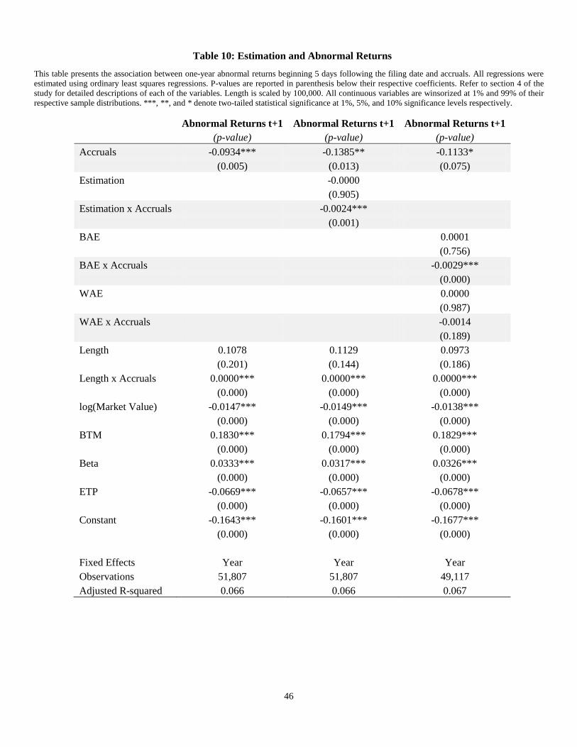
46

Table 10: Estimation and Abnormal Returns

This table presents the association between one-year abnormal returns beginning 5 days following the filing date and accruals. All regressions were estimated using ordinary least squares regressions. P-values are reported in parenthesis below their respective coefficients. Refer to section 4 of the study for detailed descriptions of each of the variables. Length is scaled by 100,000. All continuous variables are winsorized at 1% and 99% of their respective sample distributions. ***, **, and * denote two-tailed statistical significance at 1%, 5%, and 10% significance levels respectively.

Abnormal Returns t+1 Abnormal Returns t+1 Abnormal Returns t+1

(p-value) (p-value) (p-value)

Accruals -0.0934*** -0.1385** -0.1133*

(0.005) (0.013) (0.075)

Estimation

-0.0000

(0.905)

Estimation x Accruals -0.0024***

(0.001)

BAE

0.0001

(0.756)

BAE x Accruals -0.0029***

(0.000)

WAE

0.0000

(0.987)

WAE x Accruals -0.0014

(0.189)

Length 0.1078 0.1129 0.0973

(0.201) (0.144) (0.186)

Length x Accruals 0.0000*** 0.0000*** 0.0000***

(0.000) (0.000) (0.000)

log(Market Value) -0.0147*** -0.0149*** -0.0138***

(0.000) (0.000) (0.000)

BTM 0.1830*** 0.1794*** 0.1829***

(0.000) (0.000) (0.000)

Beta 0.0333*** 0.0317*** 0.0326***

(0.000) (0.000) (0.000)

ETP -0.0669*** -0.0657*** -0.0678***

(0.000) (0.000) (0.000)

Constant -0.1643*** -0.1601*** -0.1677***

(0.000) (0.000) (0.000)

Fixed Effects Year Year Year

Observations 51,807 51,807 49,117

Adjusted R-squared 0.066 0.066 0.067

47

Table 11: Estimation and Future Abnormal Returns Using Fama-French Carhart Four-Factor Alpha

This table presents the results for association between estimation and future abnormal returns using the Carhart Four-Factor Alpha. All regressions were estimated using ordinary least squares. P-values are reported in parenthesis below their respective coefficients. ***, **, and * denote two-tailed statistical significance at 1%, 5%, and 10% significance levels respectively.

Panel A: Accruals Estimation

Equal Weighted Returns

Value Weighted Returns

Accruals

Accruals

1 5 Hedge

1 5 Hedge

All Observations 0.6759** 0.0566 0.6193**

0.0697 -0.2851** 0.3548

(0.016) (0.594) (0.032)

(0.775) (0.049) (0.235)

Estimation 1 5 Hedge

1 5 Hedge

1 0.7644*** 0.0325 0.7319***

1.0640** -0.5032* 1.5672***

(0.006) (0.888) (0.001)

(0.001) (0.050) (0.000)

5 0.6637* -0.0405 0.7042**

-0.0942 0.0299 -0.1240

(0.056) (0.822) (0.028)

(0.807) (0.876) (0.780)

Difference

-0.0277

-1.6912***

(0.943)

(0.004)

Panel B: BAE and WAE

Equal Weighted Returns

Value Weighted Returns

Accruals

Accruals

1 5 Hedge

1 5 Hedge

All Observations 0.6764** 0.1067 0.5697**

0.0323 -0.2426 0.2750

(0.017) (0.594) (0.032)

(0.894) (0.163) (0.410)

BAE 1 5 Hedge

1 5 Hedge

1 0.7586*** -0.0805 0.8391***

0.4587 -0.3631 0.8218**

(0.006) (0.705) (0.000)

(0.126) (0.118) (0.017)

5 0.6833** -0.0541 0.7374**

-0.0275 -0.1932 0.1656

(0.039) (0.762) (0.020)

(0.939) (0.333) (0.682)

Difference

-0.1017

-0.6562

-(0.270)

(0.215)

WAE 1 5 Hedge

1 5 Hedge

1 0.6983** 0.2108 0.4875*

0.1813 -0.2600 0.4413

(0.031) (0.374) (0.078)

(0.652) (0.304) (0.353)

5 0.6458* 0.1799 0.4659

0.0716 -0.3486 0.4202

(0.099) (0.384) (0.139)

(0.862) (0.247) (0.426)

Difference

-0.0217

-0.0210

(0.959)

(0.976)

48

Table 12: Bootstrapped Joint Tests of Prediction 1 and Prediction 2 This table presents the results of our placebo test simulation. For each word in our estimation dictionaries we randomly choose a placebo word from the list of 10 nearest words in terms of frequency. We repeat this procedure 1,000 times and jointly test our main hypothesizes. The simulated tests follow our main hypotheses and are as follows: (P1a): Earnings x Placebo Estimation (-), P1b: Accruals x Placebo Estimation (-) and Operating Cash Flows x Placebo Estimation (I) P2: Placebo Estimation (+).

Statistical Significance Level 1% 5% 10%

(P1a) and (P1b) and (P2) 3% 6% 8% (P1a) and (P1b) 6% 9% 11% (P1b) 11% 13% 15%

49

Appendix 1: Overview of Grammatical Relationships

In this study we are interested in determining when estimation was needed by management during

the accrual generating process. Since estimation is a function of the actions taken during the accrual

generating process and not necessarily of the accruals themselves it is difficult to determine the amount of

estimation by simply examining the magnitude of a company’s accruals. For public companies the notes

to the financial statements proves a wealth of information about the accrual generating process and, more

importantly, information about the estimations needed by management.

Unlike the accruals which are denoted quantitatively, the notes to the financial statements, and

hence the information pertaining to the estimation involved, is qualitative in nature. More importantly to

assess when an estimate was needed by management we need to infer from the words and the placement

of the words in the sentence (i.e. the grammatical relationships) when an estimate was needed during the

accrual generating process.

The words and the grammatical relationships that are used in written language are not random and

are in fact highly structured. For example in the sentence “I like football.” The object “football” is the

target of “like”. Since the word “like” is conveying the enjoyment of something and “like” is targeting

“football” this linguistic cue is conveying that football is enjoyed. More over the association between “I”

and “like” denote that the person performing the action is “I”. Even though this example may be simple it

illustrates a powerful idea and provides us with a structure to help us infer meaning from the qualitative

footnotes.

To infer meaning from the footnotes we therefore need the grammatical relationships in each

sentence in the notes to the financial statements and several dictionaries of terms associated with

estimation (Appendix 2). To get the grammatical relationships in each sentence we use a technique

pioneered in the field of Natural Language Processing called Statistical Parsing to map the structure of the

sentences in the notes to the financial statements. We use a specific implementation of statistical parsing

from the Stanford Natural Language Processing Group – see http://nlp.stanford.edu/software/index.shtml

http://nlp.stanford.edu/software/index.shtml

50

for details (Marneffe et al [2006]). Essentially, this implementation finds the most likely map of the

sentence by matching the sentence to a tree bank of manually parsed sentences to find the layout of the

sentence which is most likely.

To illustrate this technique, the following sentence was parsed using the Stanford parser.

“We estimated receivables and purchased inventory.”

[nsubj(estimated-2, We-1), nsubj(purchased-5, We-1), dobj(estimated-2, receivables-3),

conj_and(estimated-2, purchased-5), dobj(purchased-5, inventory-6)]

We see that the object “receivables” is the direct object of the action (verb) “estimated”. This

linguistic cue indicates that the sentence is conveying that receivables were estimated. As illustrated,

using the grammatical relationships removes any ambiguity about the meaning of the sentence.

51

Appendix 2: Estimation Dictionaries and Grammatical Relationships

Estimation Dictionaries

We construct four dictionaries to help measure the estimation conveyed in each companies notes

to the financial statements:

Estimation Actions

Estimate, Estimating, Estimated, Anticipate, Anticipates, Anticipating, Anticipated, Approximate,

Approximates, Approximated, Approximating, Assess, Assesses, Assessed, Assessing, Believe,

Believed, Believes, Believing, Determine, Determined, Determining, Determines, Evaluate,

Evaluated, Evaluating, Evaluates, Expect, Expects, Expected, Expecting, Forecast, Forecasts,

Forecasted, Forecasting

Estimation Objects

Estimate, Estimates, Estimation, Estimations, Approximation, Approximations, Assumption,

Assumptions, Belief, Beliefs, Forecast, Forecasts

Estimation Adjectives

Estimated, Anticipated, Approximately, Expected, Forecasted, Likely, Probable

Use Words

Make, Makes, Made, Making, Use, Uses, Used, Using, Include, Includes, Included, Including

Estimation Actions are verbs which convey that an estimation action was performed (e.g. “we

estimated accruals”). Estimation Objects are estimation related objects/nouns (e.g. “we used estimates”).

Estimation Adjectives modify an object to convey that the object was estimated (e.g. “estimated

accruals”). Lastly, the Use Words dictionary contains action words which convey that something was

used or done by management.

52

Grammatical Relationships

We use the following grammatical relationships in conjunction with the Estimation Dictionaries above

to find the linguistic cues that infer that estimation was needed.

Direct Object

The accusative object of an action (i.e. “estimate receivables” or “used estimates”). For this

grammatical relationship we look for when a word from the Estimation Action dictionary targets

some object or when a word from the Use Word dictionary targets a word from the Estimation

Object dictionary. An example of the first case is “estimate receivables” here the action “estimate”

targets the object “receivables” thereby implying that receivables were estimated. An example of

the second scenario is “used estimates”. In this example one of the words from the Use Words

dictionary, “used”, targets a word from the Estimation Object dictionary, “estimates”, which

implies that they used an estimate.

(Passive) Nominal Subject

This grammatical relationship is similar to the direct object in that it relates information about an

object. This grammatical association is similar to the Direct Object and the relationships that we

look for are the same as those for the direct object.

Adjective Modifier

Adjective Modifies modify the meaning of an object (i.e. “likely receivable” or “anticipated

value”). For this grammatical relationship we find when a word from the Estimation Adjective

dictionary targets some object – this implies that the object was estimated.

Quantifier Phrase Modifier

This grammatical relationship is a modifier to a number (i.e. “approximately $100”). This

grammatical association is similar to the adjective modifier but specific to numbers. We look for

when a word from the Estimation Adjectives dictionary targets a number.

53

Noun Compound Subjects

A noun used to modify another noun (i.e. “value estimates”). This grammatical relationship is

similar to the adjective modifier except that a word from the Estimation Object dictionary is

modifying another object.

54

Appendix 3: Top 10 and Bottom 10 Accrual Accounts by Estimation

This table presents the accrual accounts with the highest and lowest coefficients on the accrual account dummies from the regression of estimation on accrual account flags. The regression was performed using OLS with an intercept as described in equation (1).

Top 10 Accrual Accounts

Fair Value

Intangibles

Derivatives

Regulatory

Restatements

Restructuring

Discontinued Operations

Segments

Accounting Changes

Contingencies

Bottom 10 Accrual Accounts

PP&E

Credit Arrangements

Long-Term Debt

Leases

Significant Customers

Inventory

Accounting Policies

Reinsurance

Taxes

Home Loan

Documents

Estimating the Estimation of Accruals · 2019-05-14 · Estimating the Amount of Estimation in Accruals . Jason V. Chen . University of Michigan . Ross School of Business . [email protected]