Crowd Size Estimation

Dillon Cariveau

I was introduced to the topic of crowd size estimation by an article in Significance

magazine and thought it was interesting to learn about all of the different implications the

number of people attending an event could have. The article cited several example of where the

size of the crowd was not only very important in some way, but hotly debated as well.

One such example was the Million Man March, a civil rights gathering in Washington in

1995. The name alone, not to mention possible racial biases, meant the size of this gathering was

going to be important. Organizers of the event say that 2,000,000 to 1,500,000 people attended.

However, the National Park Service estimated the crowd to be around 400,000 people. After

releasing that estimate, the National Park Service was threatened with legal action and no longer

gives estimates of crowd sizes. This is just one example of many were two sides do not agree on

the estimates. Often one side will report higher numbers to make their rally seem more

successful, or to show more support for certain political agendas while the other side will down

play the numbers in order to take away from the other side.

So, after reading about how much controversy crowd size estimates could cause, I wanted

to learn more about the methods that were being used to come up with these estimates.

Static Crowds

The first type of crowd is a static crowd, or a crowd that is relatively stationary usually

with a main focal point. Examples of a static crowd could include, sporting events, concerts,

political rallies or protest, or a celebration like Time Square on New Year’s Eve. In some of

these cases, such as sporting events or concerts, it is easy to count the number of people in

attendance because there are only a few entrances and they are well controlled. However, in the

case of a political rally or New Year’s at Time Square for example, it is not so easy since there

are many different entry points and there is no one scanning your ticket when you come or go.

In 1967 Herbert Jacobs proposed a fairly simple method of dealing with these cases

where estimating the size of the crowd is not as easy as counting the number of tickets sold.

Jacobs was a professor at the University of California, Berkeley and his office overlooked a

plaza where students would often gather to protest the Vietnam War. The concrete on this plaza

was conveniently marked out in to grids. This gave Jacobs the idea for his area times density

method for crowd size estimation.

Jacobs observed numerous demonstrations and collected a wealth of data that lead him to

come up with a few rules of thumb that are still used today. Jacobs determined that in a loose

crowd, where each person is about an arm’s length from their nearest neighbor, one person

would occupy 10 square feet of space. In a denser crowd, each person occupies 4.5 square feet,

and in a mosh-pit density crowd, each person occupies 2.5 square feet.

So, if you knew the area a crowd was covering and used Jacob’s rule of thumb for the

density of the crowd, simply multiplying area by density would give you an estimate of the

crowd size. However, it is not always easy to determine the exact area a crowd is covering and

the densities could vary throughout the crowd. For example, if a crowd was gathered to hear a

speaker up on a stage, we would expect the crowd to be denser towards the front of the stage and

less dense toward the back and around the edges. To deal with these issues it may be beneficial

to separate the crowds in to low, medium, and high density areas and take samples from each.

This sample method would likely give a more accurate representation of the actual number of

people in the crowd, as well as allow us to obtain an estimate of the standard error for the area

and density. If we have the standard error for area and density, and assume the two are at least

approximately independent, then we can use the delta rule to find the relative standard error for

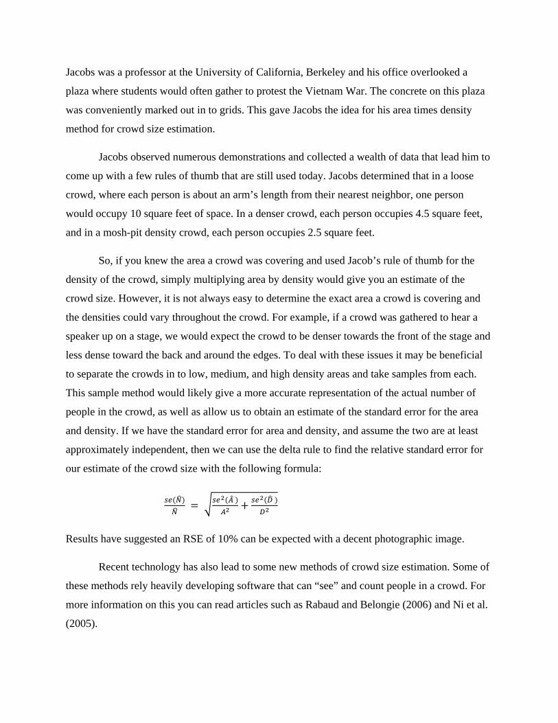
our estimate of the crowd size with the following formula:

Results have suggested an RSE of 10% can be expected with a decent photographic image.

Recent technology has also lead to some new methods of crowd size estimation. Some of

these methods rely heavily developing software that can “see” and count people in a crowd. For

more information on this you can read articles such as Rabaud and Belongie (2006) and Ni et al.

(2005).

Rob Goodier wrote an article for Popular Science magazine that detailed a method of

estimating a crowd size for a rally at the Lincoln Memorial. A company called Digital Design

and Imaging Service has taken the area times density approach and used modern technology to

improve upon it. The company started by creating a 3D model of the area where the crowd was

going to assemble and, using images from previous similar events, mapped out areas where they

expected people to gather. From previous experience, the DDIS crews have a good idea of places

that would be probable high density areas. They have found that in winter time people will

gather around wind breaks, and in summer they will tend to gather in the shade. Also, they have

found that crowds tend to assemble near the stage, as well as near Jumbotron screens, but they

seem to stay away from areas directly in from of loudspeakers. The company also looks for

places where it might be hard to see people such as under trees or around other obstructions.

After getting the lay of the land, DDIS carefully selected a location to launch a balloon

with cameras mounted on it. The balloon had a variety of cameras which took pictures from

various heights. A composite of these photos were then laid over the 3D model which allowed

the team from DDIS to count the number of people in certain grid squares and multiply by the

number of squares with a similar density. The president of the company, Curt Westergard says

that the estimate has a 10% margin of error as a benefit of the doubt, but does not give any

justification for this. However, for a rally at the National Mall in Washington, D.C., DDIS sent

their photos to Stephen Doig, a journalism professor form Arizona who has experience counting

crowds based on satellite images and other methods. Westergard and DDIS came up with an

estimate of 87,000 while Doig counted 80,000, which was within Westergard’s ten percent

margin of error.

Application of Static Crowd Estimation

I wanted to see if I could apply some of the methods that I had researched to estimate the

size of a crowd. I choose look at President Obama’s final 2012 campaign rally which took place

in Des Moines, Iowa. I choose this event for one, because it was an outdoor event so there would

be no easy way (i.e tickets or turnstiles) to estimate the crowd size, and two because I thought

that there might have been some discrepancies between what different news outlets reported for

crowd size. As it turns out, all the reports I found gave an estimate of around 20,000, but I still

thought it would be interesting to verify this number.

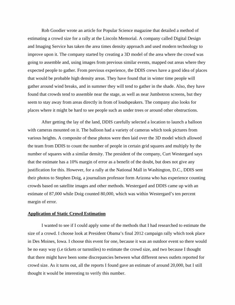
Since I did not have the time or budget to attend the rally, or the equipment to get good

high resolution photos, I had to come up with my own method that would work with the

resources I had. I started by examining pictures and videos of the event to determine the general

area the rally was taking place at. The stage was set up at intersection of East 4th Street and East

Locust Street. Below is a picture that shows a good overall view of the rally (except for a set of

bleachers behind the stage).

While this picture gives a nice view of the crowd, it is hard to tell a lot about the exact

boundaries of the crowd. To help me determine what these boundaries were, I compared points

of reference such as trees, street lights, stoplights, and buildings that I could see in other photos

and videos of the rally to the same points I could see on Google Street View and Google Earth.

Putting everything together I determine the main part of extended two blocks to where the

American flag is hung in the background.

Once I knew the boundaries of the rally and had identified certain points of reference, I

started to divide the area up in to different sections. I made decisions for where the sections

should be based on the physical layout of the location as well as by where I thought the density

of the crowd might differ. Unfortunately there were no good overhead shots of the event. Almost

every photo I found was from the front of the crowd looking down the street. This meant there

were some areas that I could not see, but from my research and the pictures that I did have I was

able to make some assumptions about those areas.

From the picture on the next page you can see how I divided the area up. I end up with 6

main areas, 6 hidden areas, and 2 sets of bleachers.

I decided main area 1 would be the intersection of E. 4th Street and E. Locust Street, right

in the front of the stage. This area also contained two sets of bleachers, one behind the stage and

one to the south. Since this was where all the cameras were, I was able to determine the

boundaries of this area easily. Also it appeared as though this area had the highest density of

people. Main area 2 extends east and fans out slightly. I was able to see a distinct edge to the

crowd that extended from the end of bleacher 2 to the corner of the building and based on other

clues from the pictures, such as portable toilets and other equipment, I determined that the

parking lot to the south of area 2 did not contain a significant amount of people. Main area 3

continues down the street and is bordered by buildings so finding its size was easy. Also, it

appeared as if the density was slight less through this area. Main area 4 was the first tricky area

since there no photos that how many people were hidden behind building going north and south

on East 5th Street. However, based on how tightly packed crowd was at that point it felt it was

safe to assume there would be a loosely packed crowd there. I called these hidden areas 1 and 2.

Also, since main area 4 was getting pretty far away from the stage, and since there was a

Jumbotron screen right behind the area that more people would probably crowd around, I

determined the density would be slightly less in this area. Main area 5 is the first area moving

down the street where participants would have been able to see the Jumbotron screen so it is safe

to assume the density would be slightly higher than in main area 4. There was another hidden

area here but again, due to the high density crowd that could be seen, it was safe to assume some

people would be in that area as well, although not as many since their view would have been

obstructed. Main area 6 had clear boundaries of buildings and since it was getting towards the

back of the rally I assumed the crowd density would be thinning. The last three areas I called

hidden areas 4, 5, and 6 since they were hidden either by the huge flag in the background or by

buildings. But, from the pictures I did have I could tell that people would be in these areas but I

did not think they would be packed in tight like they were at the front of the crowd. I all of the

hidden areas I took two measurements for the length of the area, a long and a short, to give a

smaller and larger estimate of the number of people in these areas.

After dividing the area up in to these sections and making some decisions about the

densities in the different sections I was ready to get an estimate of the crowd size. I used Jacob’s

rules of thumb for crowd densities as well as comparing pictures of similar crowds where the

densities were known to the pictures that I had. The tables below give the areas and densities of

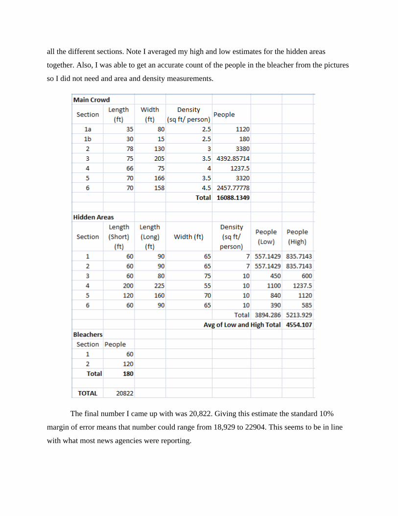
all the different sections. Note I averaged my high and low estimates for the hidden areas

together. Also, I was able to get an accurate count of the people in the bleacher from the pictures

so I did not need and area and density measurements.

The final number I came up with was 20,822. Giving this estimate the standard 10%

margin of error means that number could range from 18,929 to 22904. This seems to be in line

with what most news agencies were reporting.

Some possible shortcomings to my estimate is that there were areas of the crowd that I

could not see, so I cannot know for sure how many people were in these areas. Also, it would

have been better to sample squares from a grid and count the people in them to get more accurate

estimates for the densities. Unfortunately none of the pictures that I could find had a good

enough resolution or were at the right angle to accurately get counts of people. Despite these

factors I think that overall my estimate is pretty good and if there would have been more

controversy on the size of this event I believe my estimate could have shed some light on the

truth.

Mobile Crowds

The second type of crowd is a mobile crowd. It is much more difficult to estimate the size

of a mobile crowd than a static crowd for many reasons. In a mobile crowd, people could be

entering or leaving the crowd and many different times and in many different places throughout

the event. Also, the a mobile crowd could be much more spread out and variable than a mobile

crowd and for this reason photographs and the area times density approach will not work well.

But, in almost all cases, a mobile crowd has some defined starting point and moves along a

predetermined path towards some focus point at the end.

The most common example of a mobile crowd is a protest march, often politically

motivated such as the demonstrations that have taken place in Hong Kong every year since the

sovereignty change in 1997. Large crowd sizes at this demonstration led to a political change in

2003 and the crowd size estimates have become increasingly important in political discussions.

As discussed before, size estimates by the organizers of the march tended to be much higher than

estimates by police. An article by Yip and Watsen (2010) lay out two different methods of

estimating the size of a mobile crowd. Each of these methods were used at the Hong Kong rally

and the two were compared.

The first method was proposed by the Hong Kong University Public Opinion Program

(HKUPOP) and is called the count and follow up method. In this method, investigators chose an

inspection point, usually near the focus point at the end of the rally, at which observers count the

number of people passing by at certain time intervals. These observations are then used to get an

estimate of the total number of people in attendance. One problem with this method is that it will

miss people that left the demonstration before the inspection point, or people that joined after the

inspection point, which could lead to under counting. In order to try to account for this, the

researchers proposed using a random phone survey after the rally in which they would try to find

participants of the rally and then ask them whether or not they passed the inspection point so

they can obtain an estimate of the proportion of people who attended the rally and passed the

inspection point. However a phone survey leads to more problems. First, even in a large

demonstration, only a small proportion of the population will have been at the rally which means

it may be difficult to get a representative sample. Also, phone surveys comes with other

problems such as cost, truthfulness of the responses, allowing for clustering and household

groups, dealing with non-response, and so on. Despite all these issues, an estimate and standard

error can be obtained by this method, however Yip and Watsen propose that a different approach

they argue can yield more precise results, without the trouble of a phone survey.

The second method proposed is called the double count and spot-check method. In this

method investigators choose two different inspection points and perform a spot check survey at

the second point. The purpose of the survey is to determine the proportion of people who joined

between the first and second point. The key to this method is to choose the location of the two

inspection points carefully. Typically one of the points is chosen at the beginning of the

demonstration and the other towards the end near the focus point. However, if the first point is

too close to the starting point, it may miss a significant amount of people who joined the rally

after the inspection point and if it is too far from the start it may miss people that left before that

point. Also, if the second inspection point is to far from the focal point, it may miss people who

enter the rally after that inspection point. Still, no matter how carefully these two inspection

points are chosen there are three groups of people that will be missed by this method, they are:

1. People who leave the rally before the first inspection point

2. People who join and leave between the two inspection points

3. People who join after the second inspection point

According to the developers of this method these numbers should be negligible if the inspection

points have been chosen properly. The first group should be very small since the first point is

near the beginning. Also, it can be argued that those in the second group have not showed

significant commitment to the demonstration to be counted anyways. The third group is the most

problematic since it is possible that a significant number of people could join after the second

point in order to be a part of the events that may be taking at the focal point. However, at the

focal point the crowd would be static so the area times density methods may be applicable to

supplement the estimation. The article by Yip and Watsen compare the results of these two

methods at the Hong Kong demonstrations as well as results from an estimate obtained by

satellite imaging and show that their method of double counting and spot checking produces a

more accurate estimate with less chance for error.

Application of Double Count and Spot Check Method:

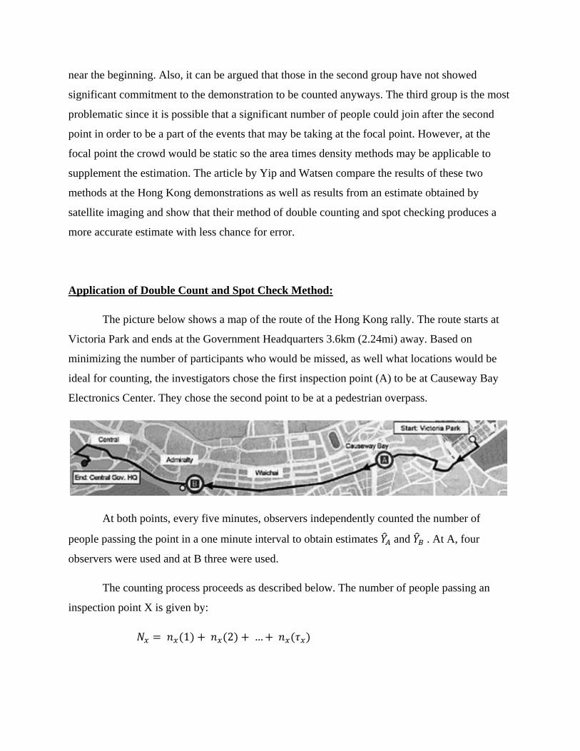
The picture below shows a map of the route of the Hong Kong rally. The route starts at

Victoria Park and ends at the Government Headquarters 3.6km (2.24mi) away. Based on

minimizing the number of participants who would be missed, as well what locations would be

ideal for counting, the investigators chose the first inspection point (A) to be at Causeway Bay

Electronics Center. They chose the second point to be at a pedestrian overpass.

At both points, every five minutes, observers independently counted the number of

people passing the point in a one minute interval to obtain estimates and . At A, four

observers were used and at B three were used.

The counting process proceeds as described below. The number of people passing an

inspection point X is given by:

1 2 …

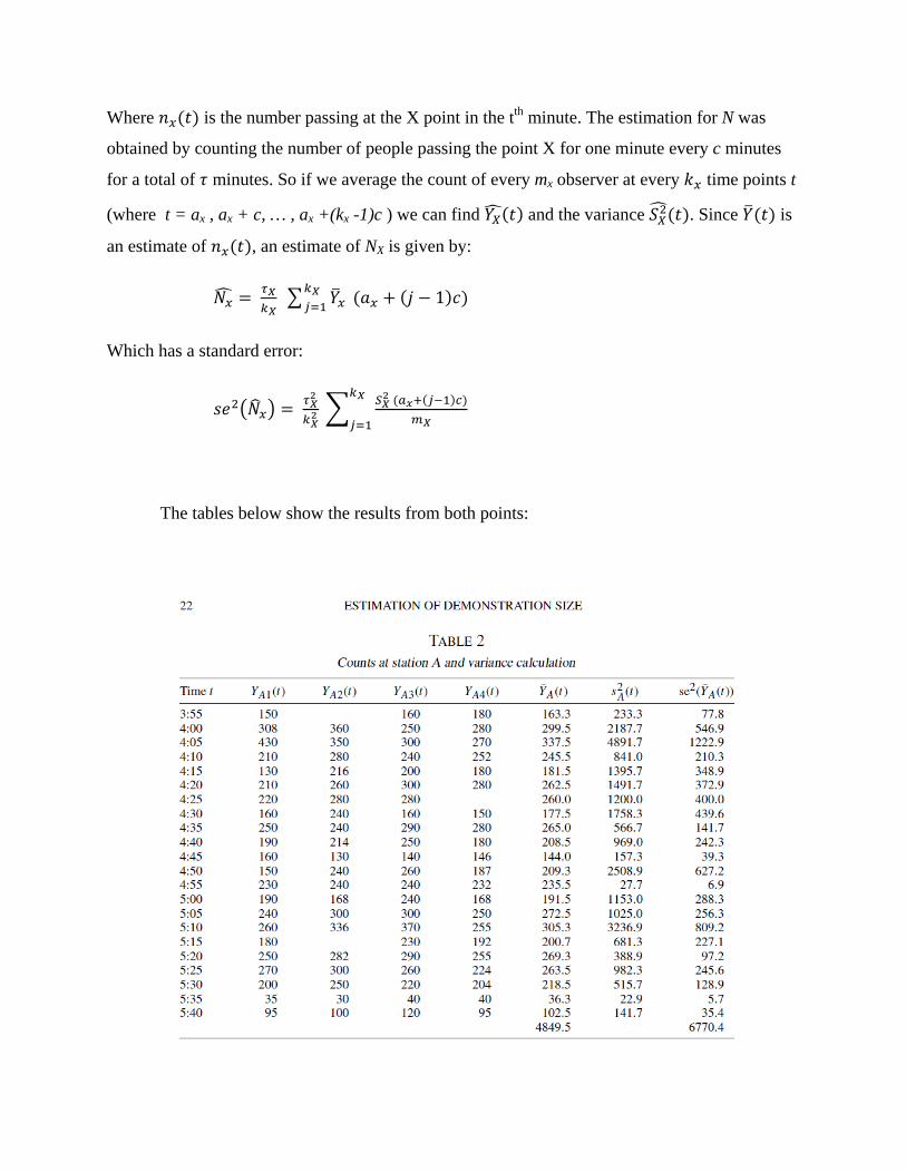
Where is the number passing at the X point in the tth minute. The estimation for N was

obtained by counting the number of people passing the point X for one minute every c minutes

for a total of minutes. So if we average the count of every mx observer at every time points t

(where t = ax , ax + c, … , ax +(kx -1)c ) we can find and the variance . Since is

an estimate of , an estimate of NX is given by:

1

Which has a standard error:

The tables below show the results from both points:

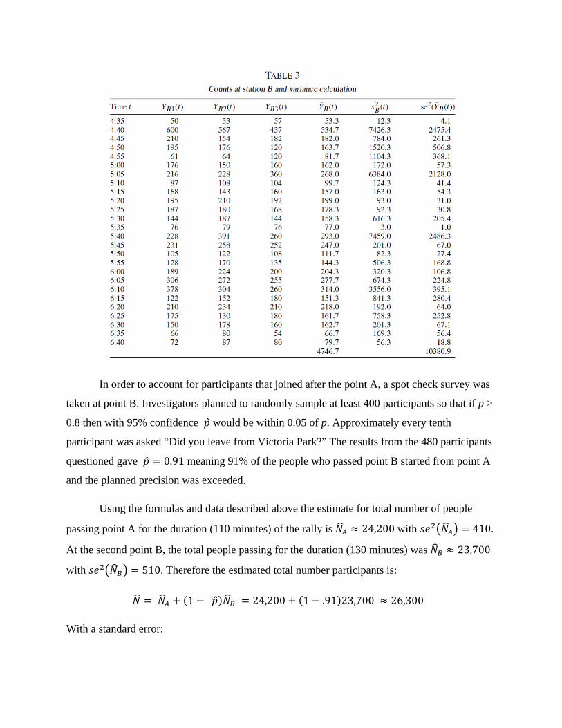
In order to account for participants that joined after the point A, a spot check survey was

taken at point B. Investigators planned to randomly sample at least 400 participants so that if p >

0.8 then with 95% confidence ̂ would be within 0.05 of p. Approximately every tenth

participant was asked “Did you leave from Victoria Park?” The results from the 480 participants

questioned gave ̂ 0.91 meaning 91% of the people who passed point B started from point A

and the planned precision was exceeded.

Using the formulas and data described above the estimate for total number of people

passing point A for the duration (110 minutes) of the rally is 24,200 with 410.

At the second point B, the total people passing for the duration (130 minutes) was 23,700

with 510. Therefore the estimated total number participants is:

1 ̂ 24,200 1 .91 23,700 26,300

With a standard error:

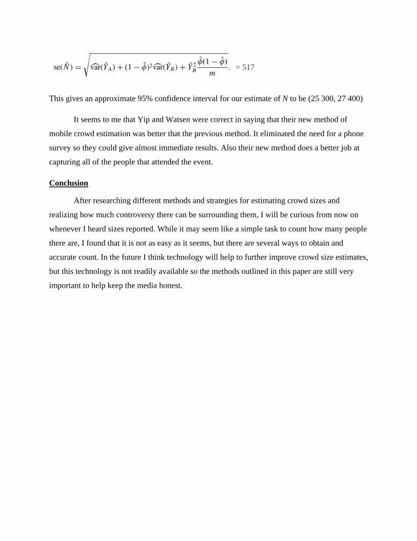
This gives an approximate 95% confidence interval for our estimate of N to be (25 300, 27 400)

It seems to me that Yip and Watsen were correct in saying that their new method of

mobile crowd estimation was better that the previous method. It eliminated the need for a phone

survey so they could give almost immediate results. Also their new method does a better job at

capturing all of the people that attended the event.

Conclusion

After researching different methods and strategies for estimating crowd sizes and

realizing how much controversy there can be surrounding them, I will be curious from now on

whenever I heard sizes reported. While it may seem like a simple task to count how many people

there are, I found that it is not as easy as it seems, but there are several ways to obtain and

accurate count. In the future I think technology will help to further improve crowd size estimates,

but this technology is not readily available so the methods outlined in this paper are still very

important to help keep the media honest.

= 517

References

Doig. S (2009) How big will the inaugural crowd be? Do the math. http://www.msnbc.msn.com/id/28662672/bs/#.UE-wUFHPjAk

Goodier, R. (2011) Curious Science of Counting a Crowd. http://www.popularmechanics.com/science/the-curious-science-of-counting-a-crowd

JACOBS, H. (1967). To count a crowd. Columbia Journalism Review 6, 36–40.

NI, L.M.,CUI, L.,LUO,Q.,NGAN,H.&ZHAO, Z. (2005). Status of the CAS/HKUST joint project BLOSSOMS. Embedded and Real-Time Computing Systems and Applications, Proceedings 11th IEEE International Conference, pp. 469–474. IEEE, Hong Kong.

RABAUD, V. & BELONGIE, S. (2006). Counting crowded moving objects. Computer

Vision and Pattern Recognition, IEEE Computer Society Conference Proceedings, 705–711. IEEE, New York.

Watson, R (2011) How many were there when it mattered? Significance. Vol 8. Issue 104-107

Yip, S. F. P., Watsen, R. et al (2010) Estimation of the number of people in a demonstration. Australian & New Zealand Journal of Statistic. 52, 17-26.