Estimating the Construction IndustryCompliance Costs for CARB’sOff-Road Diesel Vehicle Rule

Prepared byM.Cubed

On behalf ofthe Construction Industry Air Quality Coalition

May 23, 2007

Executive SummaryM.Cubed was retained by the Construction Industry Air Quality Coalition

(CIAQC) to assist in estimating the potential economic impacts on the constructionindustry from regulations proposed by the Air Resources Board to control emissions fromoff-road diesel vehicles used for construction activities. The underlying analytical tool ofthis study is an Excel spreadsheet model of fleet evolution from 2008 thru 2020 andassociated incremental costs accrued to the construction industry as it complies with theproposed ARB rule.

In 2005 the construction industry accounted for approximately 5 percent of grossstate product. The construction industry employed approximately 835,000 Californiansin 2004, representing $36 billion in payroll. Fifty-five percent of California constructionfirms have fewer than five employees, with 74 percent employing less than tenindividuals. Less than one percent of the state’s construction firms have more than 250employees. Similarly, 97 percent of all California construction firms generate less than$10 million in annual sales. Finally, several forecasts call for a decline in constructionspending in the near term, and Department of Finance data shows a significant downturn.

The construction industry also provides a larger “bang for the buck” than mostother economic sectors. For every dollar spent on construction, total output, including“multiplier impacts,” increases by $2.40. Construction produces 21.5 jobs throughout theeconomy for each million dollars added output the industry; or conversely, 21.5 jobs arelost along with each million dollars of reduced output.

On several key parameters, ARB Staff’s modeling relies on unrepresentative data orunsupported assumptions. Where the ARB Staff has chosen assumptions upon which theinformation is quite uncertain, those choices have biased the estimated costs downward:

(1) The ARB has estimated the number and composition of mobile equipment inthe off-road inventory from national surveys that do not reflect state-levelcompositions.

(2) The ARB Staff does not have an accurate count of firms falling into differentfleet class sizes, i.e., small, medium and large despite this data being availablefrom other state agencies. In addition, the ARB Staff analysis relies on anunrepresentative model fleet and appears to assume that public and privatefleets have similar compositions and purchasing patterns.

(3) The ARB models presume an annual normal retirement rate of 4.45% whilethe U.S. EPA uses 3% which is a value more consistent with industryexperience. It is also not apparent how the ARB model accounts for thenecessary introduction of new equipment to meet the higher standards.

(4) The ARB Staff estimates for new equipments are 35% to 40% lower thanquotes provided to industry firms.

(5) The proportion of the equipment fleet that can be repowered to meet Tier 2and 3 emission standards, much less achieving Tier 4 level is unknown.Answering this question is the single most important aspect of moreaccurately estimating potential costs. The ARB Staff appears to be assuming

M.Cubed

2

all equipment above 250 HP can be repowered while industry experiencesshows much less than a quarter can meet this criteria.

(6) No analysis has been conducted on how repowering engines might affectequipment life.

(7) Current industry experience shows the costs of retrofits to control PM to be50% higher than the estimates used by the ARB Staff in its analysis.

The Construction Industry Cost Model (CICM) uses a statewide basis for estimating costsrather than building up from individual fleets as the ARB Staff model does. However,the general economic principles used are similar.

The CICM was first run using the proposed regulations and the ARB Staff’s dataassumptions. The total net present value cost of the current regulatory proposal is $6.0billion over the 2009 to 2020 period, an amount twice the $3.0 to $3.4 billion for 2009 to2030 reported in the Staff’s report. The annual cost over the 2009 to 2020 period is $699million or about $276 per horsepower.

A series of scenarios were run representing changes in the ARB Staff assumptions.These scenarios indicated how sensitive the cost results are to underlying assumptionsabout parameters for which we have little or no information. Using 60% higher newequipment prices, a 75% lower proportion of the fleet that can be repowered and a 50%lower normal retirement rate—within documented industry experience and consistentwith U.S. EPA analyses—the total net present value cost rises to $13.5 billion and theannual cost to $1.58 billion. This is equivalent to $623 per horsepower. This is anincrease of 125% over the Staff estimate.

Two sensitivities were run to determine how changing the regulation might affect costs.In the first case, the turnover cap was reduced to 6% and the retrofit cap to 10%. Thisreduced costs by 16% to 39%. In the second, the compliance period was extended fiveyears with the same introduction schedule and turnover and retrofit caps. This reducedthe costs by 8% to 11%. Nevertheless, the fleet composition differed only slightly fromthe ARB Staff proposal in 2020.

We can assess whether the construction industry can pass through additional regulatorycosts based on currently available economic studies. One set of estimates was developedas part of the basis for the Dynamic Revenue Analysis Model (DRAM) used by theDepartment of Finance to estimate how fiscal changes affect projected state revenues.Based on these estimates, construction firms would bear 54 percent of the added costs.The US EPA provided estimates in its Regulatory Impact Analysis for its off-roadregulations in 2003 and construction firms bear 49 percent of the regulatory costs.

Construction firms are likely to have absorb a substantial portion of those costs throughreduced profits and/or reduced employment—likely at least half. The projected statewideemployment loss is 10,900 to 34,000 jobs using a set of reasonable and conservativeassumptions about compliance cost estimates. This represents 1.3% to 4.1% of the state’sconstruction employment.

In addition, these regulatory costs are likely to increase costs for the projects constructedthrough the bond measures authorized November 2006 by about $2.1 billion. Thisrepresents 5% of the authorized bond amounts.

M.Cubed

3

IntroductionM.Cubed was retained by the Construction Industry Air Quality Coalition

(CIAQC) to assist in estimating the potential economic impacts on the constructionindustry from regulations proposed by the California Air Resources Board to controlemissions from off-road diesel vehicles used for construction activities.

As a first step of this analysis, this report summarizes the industry’s financial status andeconomic importance, including the distribution of key economic characteristics acrossthe industry. In addition, we have developed an estimate of the distribution of fleet sizeand total horsepower linked to a measure of firm size, in this case the number ofemployees. This estimate is derived from a survey of firms that showed a highcorrelation between fleet size, number of employees and annual gross revenues.

This report then provides initial findings from our estimate of the range of potentialcompliance costs to comply with the proposed In-Use Off-Road Diesel Vehicleregulation. The underlying analytical tool of this study is the Construction Industry CostModel (CICM), an Excel spreadsheet model of fleet evolution from 2008 thru 2020 andassociated incremental costs accrued to the construction industry as it complies with theproposed ARB rule. We focus on this period because this is the one in which theproposed regulation has its most significant impact. If the analysis is extended to 2030 tomatch the latest ARB Staff analysis, the total cost would increase commensurately andsignificantly, although the annualized costs may decrease.

On several key parameters, ARB’s modeling relies on unrepresentative data orunsupported assumptions:

(1) The number and composition of mobile equipment in the off-road inventory;

(2) The split of the equipment inventory among different fleet class sizes, i.e.,small, medium and large;

(3) The difference in the composition of public versus private fleets;

(4) The current retirement and turnover rate of existing and future equipment,thus affecting the assumed expected remaining life of each equipment type;

(5) How many new vehicles must be introduced into the fleet to achieve theproposed standards, versus the assumed reliance on used vehicle purchases bythe ARB Staff;

(6) The new and resale value of off-road equipment;

(7) The proportion of the equipment fleet that can be repowered to meet Tier 2and 3 emission standards, much less achieving Tier 4 levels;

(8) The change in the expected remaining life of equipment after repowering; and

(9) The cost of retrofits for PM emissions.

The model was run across several cases and scenarios to determine the sensitivity of theanalytic results to changes in assumptions. The model’s premise is that most if not allfirms will need to turnover their fleets at the turnover cap rate to comply with the rule.

M.Cubed

4

This is based on preliminary analysis of several private fleets, including newer ones,carried out by CIAQC members. A base case was run using much of the ARB Staff’smodeling assumptions.1 Then scenarios were run changing key assumptions about newequipment costs, proportion that can be repowered and the underlying turnover rate. Inaddition cases were run with a reduced turnover cap of 6% (versus the Staff’s 10% after2014) and retrofit rate of 10% (instead of 20%), and extending the compliance dates byfive years.

Finally, we derived the share of costs to that are likely to be borne by constructionfirms from the new regulations. Based on two different studies, these firms will absorbabout half of these costs, unable to pass them through to customers. A portion will berealized in reduced profits, while the remainder likely will result in lost jobs in the sector.

The Construction Industry’s Importance to Californiaand Its Sensitivity to Changing Costs

California’s construction industry is responsible for a significant share of thestate’s economic activity. In 2005 the sector accounted for approximately 5 percent ofgross state product.2 The construction industry employed approximately 835,000Californians in 2004, representing $36 billion in payroll.

The construction industry also provides a larger “bang for the buck” than mostother economic sectors. For example, for every dollar spent on construction, total output,including “multiplier impacts,” increases by $2.40. Only the insurance and hotel sectorshave higher output multipliers. Likewise, at 76 cents construction’s earnings multiplier ishigher than all sectors except services; and the sector’s job multiplier, 21.5, is greaterthan any other industry except agriculture and services.3 In other words, constructionproduces 21.5 jobs throughout the economy for each million dollars added output theindustry; or conversely, 21.5 jobs are lost along with each million dollars of reducedoutput.

Despite the economic significance of the state’s construction sector, it isextremely sensitive to economic cycles, as well as changes in input prices. For example,during the 2000-2001 recession the number of construction firms declined by 2 percent,and total employment dropped by more than 1 percent nationwide.4 As shown in Figure1, spending on construction is expected to decline in 2007, followed by modest growthbetween 2008 and 2011. Of particular interest is that the growth trend is expected to shiftdownward compared with historic patterns, as shown in the chart.

1 CARB Staff, Staff Report: Initial Statement of Reasons for Proposed Rulemaking, Mobile Source ControlDivision, Heavy Duty In-Use Strategies Branch, April 4, 2007.2 U.S. Department of Commerce, Bureau of Economic Analysis, www.bea/doc.gov.3 California Economic Strategy Panel, Using Multipliers to Measure Economic Impacts, 2002.4 U.S. Census Bureau, County Business Patterns, April 10, 2003.

M.Cubed

5

Figure 1

Slower Growth Seen for California's Construction Industry

$94,815

$101,906

$126,220

$133,114

$140,924

$149,771

$159,581

$112,915

$90,034$86,760

$76,847

$128,596$125,069

y = 7494.3x - 666050R2 = 0.9754

$0

$20,000

$40,000

$60,000

$80,000

$100,000

$120,000

$140,000

$160,000

$180,000

1999 2000 2001 2002 2003 2004 2005 2006 2007 2008 2009 2010 2011

Mill

ions

of D

olla

rs

Actual Forecast Trend Forecast

Construction input prices, including equipment costs, jumped by 30 percentbetween 1996 and 2003, contributing to rapidly increasing housing prices in the state.5For example, the share of first-time buyers in California declined to their second lowestlevel last year, dropping from 31 percent in 2005 to 27 percent in 2006. Likewise, theshare of California buyers who relied on a second mortgage rose from 38 percent in 2005to 43 percent in 2006, more than tripling since 2001, and the highest percentage since1982.6

The sector’s vulnerability is in part due to the fact that it is dominated by smallfirms. Fifty-five percent of California construction firms have fewer than five

5 U.S. Census Bureau, op. cit.6 California Association of Realtors (2006).

M.Cubed

6

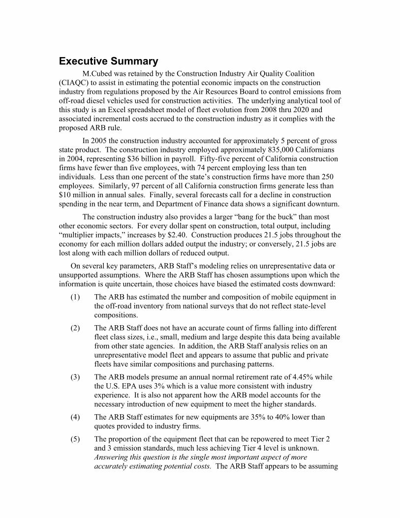
employees; with 74 percent employing less than ten individuals.7 Less than one percentof the state’s construction firms have more than 250 employees. Figure 2 illustrates thisfirm distribution. Similarly, 97 percent of all California construction firms generate lessthan $10 million in annual sales.8

7 Employment Development Department, Labor Market Information Division, 2007,http://www.labormarketinfo.edd.ca.gov/cgi/databrowsing/?PageID=67&SubID=1388 Ibid.

M.Cubed

7

Figure 2

Number of California Construction Firms by Employee Size (2005)

0-4 55.2%

5-9 18.9%

10-19 12.5%

20-49 8.7%

50-99 2.9%

100-249 1.4%

250-499 0.3%

500-999 0.1%

1000+ 0.03%

0-4 5-9 10-19 20-49 50-99 100-249 250-499 500-999 1000+

Similar to the agricultural sector – particularly commodities such as lettuce andother produce -- the construction sector tends to be subjected to extreme fluctuations inprofitability. Net profits for an individual firm can bounce from more than 20 percent ofrevenues in one year to a negative return in the next, depending on economic conditions,the weather, and fuel and other input costs. On average net profits after tax tend to rangefrom between 3 to 5 percent.9 Fluctuations in profit, combined with generally modestmargins, results in most construction firms being extremely dependent on access to short-term capital to operate their business (see below).

Regulations Could Reduce Construction Firms’—ParticularlySmaller Businesses’—Access to Necessary Credit

As with agriculture, construction firms are highly dependent on short-term credit(e.g., credit lines) to finance their operations (i.e., working capital). Access to credit isdetermined by the health of an individual firm’s balance sheet; cash flow; existing debtload; and year-to-year profitability. The proposed regulations could adversely impactconstruction firms’ access to credit as a result of several factors, particularly for smallbusinesses, which tend to have a lower margin for error. According to a recent study forthe U.S. Small Business Administration, smaller firms bear a higher burden of regulatory

9 Risk Management Associates, Annual Statement Studies – Financial Ratio Benchmarks, 2005-2006.

M.Cubed

8

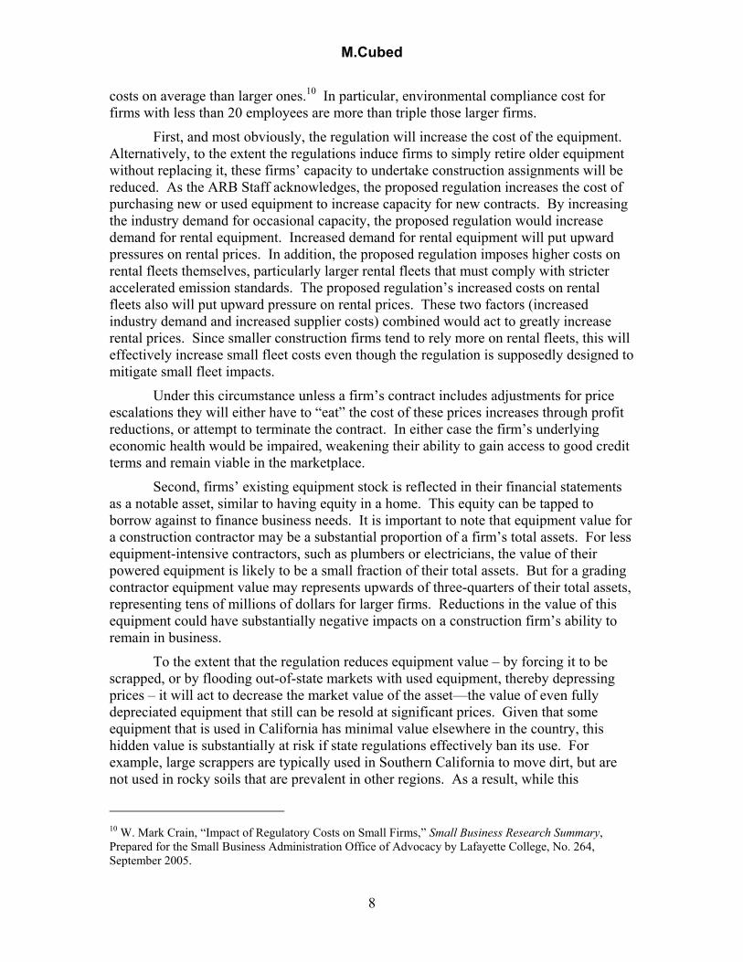
costs on average than larger ones.10 In particular, environmental compliance cost forfirms with less than 20 employees are more than triple those larger firms.

First, and most obviously, the regulation will increase the cost of the equipment.Alternatively, to the extent the regulations induce firms to simply retire older equipmentwithout replacing it, these firms’ capacity to undertake construction assignments will bereduced. As the ARB Staff acknowledges, the proposed regulation increases the cost ofpurchasing new or used equipment to increase capacity for new contracts. By increasingthe industry demand for occasional capacity, the proposed regulation would increasedemand for rental equipment. Increased demand for rental equipment will put upwardpressures on rental prices. In addition, the proposed regulation imposes higher costs onrental fleets themselves, particularly larger rental fleets that must comply with stricteraccelerated emission standards. The proposed regulation’s increased costs on rentalfleets also will put upward pressure on rental prices. These two factors (increasedindustry demand and increased supplier costs) combined would act to greatly increaserental prices. Since smaller construction firms tend to rely more on rental fleets, this willeffectively increase small fleet costs even though the regulation is supposedly designed tomitigate small fleet impacts.

Under this circumstance unless a firm’s contract includes adjustments for priceescalations they will either have to “eat” the cost of these prices increases through profitreductions, or attempt to terminate the contract. In either case the firm’s underlyingeconomic health would be impaired, weakening their ability to gain access to good creditterms and remain viable in the marketplace.

Second, firms’ existing equipment stock is reflected in their financial statementsas a notable asset, similar to having equity in a home. This equity can be tapped toborrow against to finance business needs. It is important to note that equipment value fora construction contractor may be a substantial proportion of a firm’s total assets. For lessequipment-intensive contractors, such as plumbers or electricians, the value of theirpowered equipment is likely to be a small fraction of their total assets. But for a gradingcontractor equipment value may represents upwards of three-quarters of their total assets,representing tens of millions of dollars for larger firms. Reductions in the value of thisequipment could have substantially negative impacts on a construction firm’s ability toremain in business.

To the extent that the regulation reduces equipment value – by forcing it to bescrapped, or by flooding out-of-state markets with used equipment, thereby depressingprices – it will act to decrease the market value of the asset—the value of even fullydepreciated equipment that still can be resold at significant prices. Given that someequipment that is used in California has minimal value elsewhere in the country, thishidden value is substantially at risk if state regulations effectively ban its use. Forexample, large scrappers are typically used in Southern California to move dirt, but arenot used in rocky soils that are prevalent in other regions. As a result, while this

10 W. Mark Crain, “Impact of Regulatory Costs on Small Firms,” Small Business Research Summary,Prepared for the Small Business Administration Office of Advocacy by Lafayette College, No. 264,September 2005.

M.Cubed

9

equipment has significant value in California under the status quo, it may be virtuallyworthless elsewhere in the U.S. Reductions in a firm’s equipment value would serve tolessen the firm’s net worth, with a concomitant decline in their ability to obtain goodborrowing terms, and more importantly, reduce borrowing and bonding capacity forinvesting in such things as new, cleaner equipment.11

Third, firms that elect to replace older equipment with government-sanctionedmodels will either need to dip into their cash reserves or obtain loans to pay for the newcapital. If relying on cash results in a significant decline in available reserves it couldlead to increased borrowing costs. In addition, the capacity of construction equipmentsuppliers to ramp-up production of new model equipment, particularly if the replacementengine technology is not fully conceived and developed, is constrained. If the regulationscause a noticeably longer back-log in equipment delivery this in turn could reduce firms’ability to effectively complete projects, with associated impacts on cash flows as well asrisks of profit reductions in cases where contracts include schedule delay-relatedpenalties. For example, since last fall construction firms have had to wait up to fourmonths for equipment delivery.12

It is also important to note that many firms, particularly smaller businesses, relyon the used equipment market rather than purchasing new. Yet under the regulation themarket for used equipment within would shrink substantially; only newer models willmeet the air quality requirements and current owners would retain Tier 2 and 3 models tomeet the various standards . As a result, firms accustomed to paying lower prices forsecond- or third-hand equipment – with associated access to available credit -- reflectingthe partially depreciated nature of used equipment, will be forced to noticeably increasetheir expenditures on a given piece of equipment. This, in turn, will lead to firms goingout of business, and result in an overall reduction in the number of businesses operatingin the sector, with concomitant increases in firm concentration in the industry. Suchadjustments are well-known to reduce competition and to lead to higher market prices.One of the hallmarks of the 2000-2001 statewide electricity crisis was the concentrationof generators which lead to well-documented market abuses.13

Overall the value of a contractor’s equipment is a substantial factor in their abilityto conduct business. If this value is adversely impacted, construction firms’ ability toremain economically viable could be compromised.

11 A more extensive discussion of these impacts was presented by Ralph Potter, CIT Construction,Specialty Finance Affiliate of the CIT Group, New York, at “California Emissions: Where do you standwith the proposed Regulations?” March 27, 2007.12 Jim Haughey, “U.S. Equipment Buying Slows, While Exports Increase,” Construction EquipmentMarket Update, 2006.13 Richard J. McCann, “’The Perfect Mess’: How California's Energy Markets Sank” (paper presented atthe Western Economics Association International Meeting, Seattle, Washington, June 2002).

M.Cubed

10

Characterizing the State’s Construction Fleets Based on CIAQCSurvey Responses

Although the broad direction of adverse economic impacts can be described (seeabove), it is difficult to accurately estimate the regulation’s precise potential impact onthe construction sector. This is because little data exists on individual firmcharacteristics, or the linkage between these characteristics, financial health, andequipment fleet size and type. To address this data gap CIAQC collected survey datafrom its members related to 2005 annual gross revenues, number of employees, and thecharacteristics of their fleets that would be regulated under the proposal.

Twenty-one firms responded at least in part to the survey. These responses wereused to identify statistical relationships between number of employees, firm revenues andequipment fleet characteristics.14 Regression models for each relationship wereestimated; parameter estimates for the mean were used in the subsequent analysisestimating typical firm revenues and fleet characteristics across the industry, along withhigh and low estimates based on the 95% confidence interval derived from the sampledata.

Employment data for the construction industry was collected from the CaliforniaEmployment Development Department (EDD) Labor Market Information website.EDD’s data shows the number of construction firms and associated number of employeesin the third quarter for 2005 by firm size categories.15 The estimates of the relationshipbetween number of employees, firm revenues, and equipment fleet characteristics fromthe survey analysis were then applied to the EDD data to estimate the statewide range ofannual revenues, fleet sizes and total horsepower within each firm size category.

14 Of particular note were the high correlations between these measures, with the R2 exceeding 0.96 out of1.0 in all cases. The correlation coefficient measures how close of a relationship exists between twovariables, with a positive correlation showing a positive relationship. An R2 of 1.0 indicates a perfectrelationship between two variables, i.e., they vary in tandem together. The high correlation for the CIAQCsurvey provided substantial confidence that number of employees was a strong indicator of firm revenues,number of vehicles and total horsepower in the fleet.15 We assumed that most firms in the NAICS 236 and 237 categories would possess regulated constructionequipment, but that only a portion—21%— of NAICS 238 (special trades) would use such equipment.(U.S. Census, “Sector 23: Construction: Industry Series: Employment Statistics for Establishments byState: 2002”, 2007.) US Census data counts 23% of sector 238 employees in these firms. Thus, theestimates presented here represent a smaller segment of the construction industry than the full NAICS 23sector.

M.Cubed

11

Figure 3 shows the distribution of annual gross revenues across firm size. Firmswith less than 100 employees – 98 percent of the industry -- average less than $13 millionof gross revenues a year.

Figure 3

California Construction Industry Estimated Firm Average 2005 Gross Revenues by Employee Size (Millions $)

$0

$50

$100

$150

$200

$250

$300

High Parameter Estimate $0.32 $1.4 $2.8 $6.3 $14.4 $32 $71 $158 $248Low Parameter Estimate $0.25 $1.1 $2.2 $4.8 $11.0 $24 $54 $121 $190Mean Parameter Estimate $0.29 $1.2 $2.5 $5.6 $12.7 $28 $63 $139 $219

0-4 5-9 10-19 20-49 50-99 100-249 250-499 500-999 1000+

M.Cubed

12

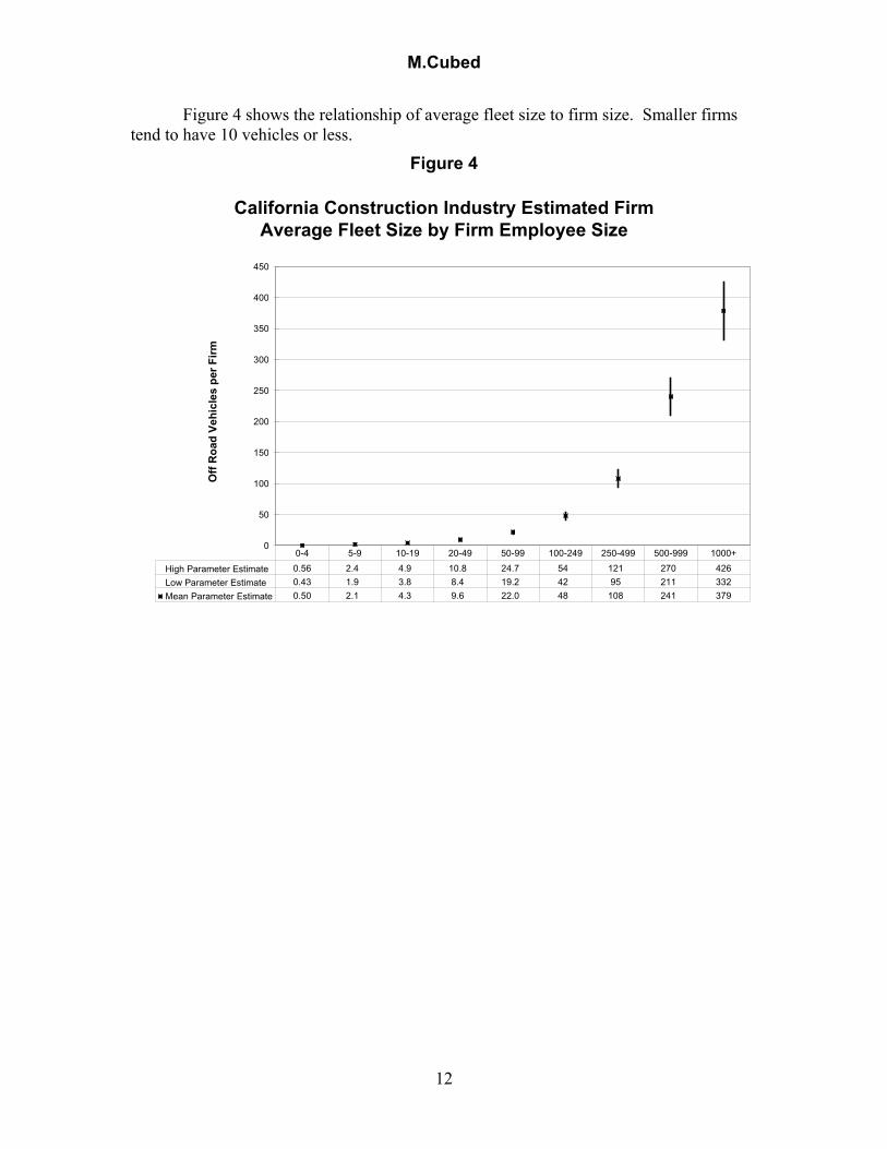
Figure 4 shows the relationship of average fleet size to firm size. Smaller firmstend to have 10 vehicles or less.

Figure 4

California Construction Industry Estimated Firm Average Fleet Size by Firm Employee Size

0

50

100

150

200

250

300

350

400

450

Off

Roa

d Ve

hicl

es p

er F

irm

High Parameter Estimate 0.56 2.4 4.9 10.8 24.7 54 121 270 426Low Parameter Estimate 0.43 1.9 3.8 8.4 19.2 42 95 211 332Mean Parameter Estimate 0.50 2.1 4.3 9.6 22.0 48 108 241 379

0-4 5-9 10-19 20-49 50-99 100-249 250-499 500-999 1000+

M.Cubed

13

Figure 5 shows the average horsepower in each firm’s fleet by size category.Firms with 20 to 49 employees average between 1,057 and 1,772 total HP, indicating thatfirms this size and larger, up to 100 employees, are likely to be captured in the medium-sized fleet portion of the regulation, which covers fleets between 1,500 HP and 5,000 HP.Companies with more than 100 employees are the likely candidates for the large-fleetregulations.

Figure 5

California Construction Industry Estimated Firm Average Fleet Horsepower by Firm Employee Size

0

10,000

20,000

30,000

40,000

50,000

60,000

70,000

80,000

90,000

Flee

t Hor

sepo

wer

per

Firm

High Parameter Estimate 89 365 758 1,772 4,455 10,132 22,650 49,673 81,348Low Parameter Estimate 78 319 663 1,548 3,893 8,853 19,790 43,400 71,076Mean Parameter Estimate 83 342 710 1,660 4,174 9,492 21,220 46,536 76,212

0-4 5-9 10-19 20-49 50-99 100-249 250-499 500-999 1000+

M.Cubed

14

Figure 6 shows how the total fleet horsepower is distributed among the firm sizesbased on the approximation derived from this analysis. Firms with less than 20employees, which are the most likely to own “small” fleets less than 1,500 HP, controlabout 28 percent of the horsepower. Firms larger than 100 employees, which are mostlikely to own “large” fleets of more than 5,000 HP, control about 36 percent of the totalstatewide horsepower. The firms with 20 to 100 employees control the remaining 36percent that are likely to fall into the “medium” category.

Figure 6

California Construction Industry Total Fleet Horsepower by Firm Employee Size

0-4 7.2% 5-9

9.1%

10-19 12.0%

20-49 19.0%50-99

16.2%

1000+ 2.3%

500-999 5.7%250-499

9.8%

100-249 18.7%

0-4 5-9 10-19 20-49 50-99 100-249 250-499 500-999 1000+

This analysis was done with publicly-available EDD data on firm characteristics.A more refined analysis that could better characterize the distribution of fleetcharacteristics could be done with firm-specific EDD data. As a state agency the ARBcould gain access to these data, with firm names obscured, and then be able to moreprecisely estimate the range of fleet characteristics and resulting regulatory impacts onthe industry. The ARB could determine more accurately how many firms will qualify as“small” businesses, the distribution of financial characteristics in the industry, therelationship of employment force to financial characteristics and other importantparameters for measuring the distribution of regulatory costs and impacts. In addition,this data can be used in concert with other analyses on other proposed regulations todetermine the cumulative impacts of recently enacted and proposed regulations on theindustry.

M.Cubed

15

The Analytic Steps for Estimating Compliance CostsThe objective research question is: What is the net present value of the fiscal costs

to the construction industry from complying with ARB’s proposed in-use off-road dieselvehicle rule? We estimated compliance costs by constructing an Excel spreadsheetmodel and then simulating several scenarios determined by values chosen for inputparameters. The Construction Industry Cost Model (CICM) is described in more detail inthe Appendix.

Estimating Fleet Composition ChangesThe CICM represents the state fleet as a whole, rather than attempting to aggregate up

from a set of “representative” firms’ fleets as the ARB Staff did. The CICMdifferentiates the statewide fleet proportionally based on the firm size representations thatM.Cubed estimated from a survey of CIAQC members and extrapolating that to the EDDstatistics on firm characteristics.16 These differentiations are used to introduce differentregulatory components over the 2009 to 2020 period.

The CICM then calculates the costs of compliance by assuming one of two actionsoccur during the year:

Based on analysis by Justice and Associates about the turnover required tomeet the individual fleet targets, Tier 0 and Tier 1 equipment is turned over orretrofitted to comply with phase out targets of 2012 for Tier 0 and 2014 forTier 1, and Tier 2 and Tier 3 are then turned over or retrofitted to comply withphase out targets of 2020, OR

The total fleet turnover and retrofit rates are constrained to the ARB Staffproposals by fleet size.

These actions reflect the decision tree summarized by the ARB Staff that look first toturning over to comply with the NOx standards, and then retrofitting to comply with PMstandards. Equipment less than 10 years old is exempt from the turnover requirement andthat less than five years old is exempt from the retrofit requirement. Based on analysisconducted on individual fleets by CIAQC members and Justice and Associates, weassume that no firms can comply with the fleet emission standards and must instead meetthe turnover cap. This is an outer bound assumption, but we do not have sufficientinformation from the ARB Staff to derive a more refined estimate. Nevertheless, theturnover and retrofit rates can be changed to reflect the ARB Staff’s assessment of thatrate from its own modeling when those detailed results are made available.

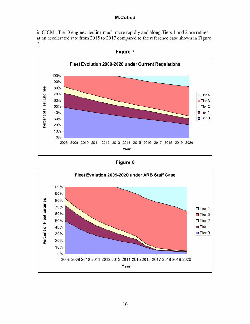
Figure 7 shows the projected fleet composition from the model assuming no newregulations are added. Figure 8 shows the fleet composition by engine tier and yearderived from the ARB Staff’s assumptions for the proposed regulations as implemented

16 The breakdown is 11% is in small firms’, 36% in medium firms’, and 53% in large firms’ fleets. Thesevalues differ from the EDD breakdowns above because the small fleet definition includes not only a limiton total horsepower, but also on total annual revenues based on the definition of “small constructionbusinesses” in the state code. In comparison the ARB Staff estimate appears to be 2.6% for small, 4.6% formedium and 92.7% for large based on the tables in its Technical Supplement.

M.Cubed

16

in CICM. Tier 0 engines decline much more rapidly and along Tiers 1 and 2 are retiredat an accelerated rate from 2015 to 2017 compared to the reference case shown in Figure7.

Figure 7

Fleet Evolution 2009-2020 under Current Regulations

0%

10%

20%

30%

40%

50%

60%

70%

80%

90%

100%

2008 2009 2010 2011 2012 2013 2014 2015 2016 2017 2018 2019 2020

Year

Perc

ent o

f Fle

et E

ngin

es

Tier 4Tier 3Tier 2Tier 1Tier 0

Figure 8

Fleet Evolution 2009-2020 under ARB Staff Case

0%

10%

20%

30%

40%

50%

60%

70%

80%

90%

100%

2008 2009 2010 2011 2012 2013 2014 2015 2016 2017 2018 2019 2020

Year

Perc

ent o

f Fle

et E

ngin

es

Tier 4Tier 3Tier 2Tier 1Tier 0

M.Cubed

17

Problems with the ARB Staff Report MethodologyAn important issue not discussed adequately in the ARB Staff Report or its

Technical Supplement is how the model extrapolates from the individual 22 fleets up tothe statewide fleet. At least two salient issues are unanswered:

The Staff assumes that fleets will continue to buy equipment in the sameproportion of new and used as they have in the past. However, to meet the higheremission targets, more new equipment of Tier 3 and Tier 4 levels will have to beintroduced into the statewide fleet. To achieve this means that individual fleetswill have to buy a higher proportion of new equipment than in the past. The StaffReport fails to discuss how this rebalancing of purchasing practices has beenaccomplished.

The report appears to draw from a mixed sample of public and private fleetswithout regard to the relative proportion that each represents of the statewidefleet. Yet, as stated in the TIAX 2003 report, public fleets rely mostly on newvehicle purchases, and thus are much more likely to have newer equipment thanprivate fleets.17 Because the samples were not weighted for their relative sharesof the statewide fleet, this introduces a significant bias toward underestimating theage of the fleets, and thus underestimating potential costs statewide.

Estimating Compliance CostsSeveral cost categories are relevant. Not all of these components are directly representedin the model, but are captured implicitly:

- Additional purchase cost of new equipment with emissions controls

o Capital cost incurred earlier

o Capital is more expensive with emissions controls

o Depreciation period starts sooner, thereby accelerating purchase of thesecond set of new vehicles

- Accelerated repowering with retrofitting

- Additional retrofitting on equipment not repowered or replaced

- Additional O&M costs of the equipment

o Maintenance of VDECS or other emissions controls

o Reduced fuel efficiency associated with VDECS

o VDECS failures and replacements

o ARB rule compliance reporting

17 TIAX, California Public Fleet Heavy Duty Vehicle and Equipment Inventory, Final Report, Reference75446/D0105, TIAX Report FR-03-113, Cupertino, California, March 17, 2003, p. 5-7.

M.Cubed

18

It was not analytically tractable to address all of these cost categories explicitlydue to complexity, data and time limitations, and/or uncertainties that render quantitativefindings unreliable.

The CICM reflects the costs of complying by replacement, repowering and/orretrofitting. The replacement costs are computed as the difference between (1) replacinga machine over three replacement cycles without the regulation and (2) shifting the threereplacement cycles forward by the expected remaining life that the machine would havehad if it was not retired prematurely due to the regulation. Thus, replacing oldermachines is less expensive than replacing newer ones.

An important difference with the ARB Staff model reflects that use of a statewideperspective instead of individual fleets. The ARB Staff assumes that an individual fleetowner can recoup some of the replacement costs by selling the older piece of equipment.However, this logic does not hold when applying to the statewide fleet. The acceleratedpurchase of a new machine leads to a chain of transactions that net to the purchase of anew piece equipment. For example, the sequence would occur as follows for one suchregulation-induced purchase:

Firm A buys a new Tier 3 scraper for $1 million to comply and sells itolder Tier 2 scraper for $500,000.

Firm B buys Firm A’s Tier 2 scraper to comply and sells its Tier 1 for$250,000.

Firm C buys Firm B’s Tier 1 scraper to comply and sells its Tier 0 for$50,000.

Finally, Firm D buys Firm C’s Tier 0 scraper and retires its older Tier 0for a nominal salvage value.

Tracing through this sequence we see the total net cost across all of the fleets is$1,000,000 minus a nominal salvage value. Thus, the replacement cost from a statewideperspective is essentially the full cost of a new machine.

Repowering costs vary by whether the new engine will meet the Tier 2 or 3standard versus Tier 4. The ARB Staff and Justice and Associates have arrived atroughly similar estimates and differences. However, the estimate of what might berepowered differs substantially. The ARB Staff apparently presumes that all equipmentlarger than 250 HP can be repowered based on the single template model it provided toCIAQC and its Technical Supplement; however Justice and Associates and CIAQCmembers have documented a much restricted list of equipment that can be repowered.For the ARB Staff base case presented here, the analysis used 100% repowering as therepresentative option. If the net replacement cost is less than that for repowering due tothe advanced vintage of the equipment cohort, then the replacement cost is used.

How the life of the equipment is affected by repowering has not been addressed,and that aspect is ignored in both the Staff analysis and the CICM. Nevertheless, anyadjustment would lead to increased costs since repowering is presumed to extend life thesame amount as replacement in both analyses.

M.Cubed

19

The repowering and replacement options are merged to estimate the turnovercosts. A weighted average of the least cost option is computed for each piece ofequipment and each year of vintage. Repowering is less costly than replacement for mostof a machine’s life until the point that the replacement cycle costs fall below repowering.The turnover cost equals a weighted average of the minimum cost between repoweringand replacement for percentage that can be repowered and the cost of replacement for theremainder. For the ARB Staff base case, the repowered percentage is assumed to be100%.

Substantial uncertainty exists over retrofit costs and how those may change overtime. This analysis uses $63 per horsepower for the ARB Staff base case using the Level3 controls for 175 to 400 HP engines. However, recent installations have cost closer to$100 per HP. Even so, the total cost estimates are relatively insensitive to changes in theretrofit costs because so many vehicles must turnover to comply with the regulations,thus obviating the need for retrofits.

The analysis uses an increase in operating and maintenance costs of $21 per HPnet present value based on the amount report in the ARB Staff’s April 4, 2007 report (p.41).

The total net present value cost of the current regulatory proposal using the ARBStaff assumptions is $5.96 billion over the 2009 to 2020 period, compared to the $3.0 to$3.4 billion for 2009 to 2030 reported in the Staff’s report. The annual cost over the2009 to 2020 period is $699 million. This amounts to $276 per hp for existingequipment.

Modeling Parameter and Data UncertaintiesSeveral key modeling assumptions and input data require further vetting to

increase confidence in modeling results. Using local18 sensitivity analysis, we mayidentify several variables with significant influence on results, including:

Fleet growth rate due to industry growth. We use ARB Staff’s suggested growthrate of 1.95% per year, but a deviations from that growth rate could haveunknown effects.

Fleet natural retirement rate. Whereas EPA suggests normal retirement rates of3% per year, we derived from average annual retirement rate using survivorshiprates provided by ARB of 4.45%. The ARB retirement rate does not differ byhorsepower despite industry experience that large machines tend to last longer. Ascenario was run using an underlying 3% retirement rate.

New equipment prices. The ARB Staff estimated resale prices from two auctionhouse websites. However, a comparison of the ARB’s new machine prices wasmade with three new equipment price lists compiled by CIAQC members. Thefirms’ reported prices averaged 55% to 65% higher than the ARB Staff estimates.Scenarios were run with new machine prices 60% higher than the Staff estimates.

18 Changing one parameter value while holding all others constant.

M.Cubed

20

The proportion of the existing fleet that can be repowered. As discussed above,only a portion of the fleet can be converted. Based on an optimistic assessment,scenarios included an assumption that 25% of the fleet could be repowered.Existing data indicate that the actual rate may be substantially lower.

The discount rate is always an influential parameter, especially when costs orbenefits occur far in the future. We used a real discount rate of 4.5% to reflect thelack of inflation adjustments in CICM model.19

Comparing Compliance Cost EstimatesFigure 9 compares the fleet compositions in 2020 for the different scenarios from

the CICM. The base case shows the breakdown by tier if the regulation is not adopted.This reflects a 4.45% retirement rate. The ARB Staff Case reflects the same retirementrate with the turnover and retrofit requirements discussed above. The final scenarioreflects the results when the retirement rate is dropped to 3% and the proportionrepowered is reduced to 25% along with an increase in new equipment prices of 60% toreflect CIAQC data. The latter two cases differ little because the turnover requirementsdrive the fleet to similar endpoints.

19 Equals 7% nominal rate used by the ARB Staff minus a 2.5% inflation rate derived from the embeddedforecast in 20 year U.S. Treasury bond yield rates. We cannot determine from the ARB Staff Report as towhether the underlying cost assumptions were properly escalated for inflation over the study period.

M.Cubed

21

Figure 9

Ref

eren

ce C

ase

AR

B S

taff

Cas

e

CIA

QC

Cas

e

Tier 0

Tier 1

Tier 2

Tier 3Tier 4

0%

10%

20%

30%

40%

50%

60%

% o

f Tot

al F

leet

Scenario

Engine Tier

Comparison of Off Road Fleet Composition in 2020

Tier 0 21.1% 3.0% 2.9%Tier 1 9.6% 0.6% 0.5%Tier 2 4.3% 0.8% 1.2%Tier 3 47.7% 59.6% 59.9%Tier 4 17.3% 36.1% 35.6%

Reference Case ARB Staff Case CIAQC Case

Figure 10 compares the cost impacts for changing key assumptions in CICM. Thefirst scenario shows the ARB Staff case results. The second one adds a lower underlyingretirement rate based on U.S. EPA assumptions, but still allows for 100% repowering ofthe fleet above 250 hp where economic. This increases costs by 31%. The third reduces

M.Cubed

22

the proportion of the fleet that can be repowered to 25% with the lower turnover rate.This increases costs 45% above the ARB Staff estimate. The final scenario increasesnew equipment purchase costs by 60% to be more consistent with data from three privatefleets pricing replacement purchases. This increases the costs 126% over the estimateusing Staff assumptions. This last scenario costs $1.58 billion annually.

Figure 10

$0

$2

$4

$6

$8

$10

$12

$14

$ B

illio

n N

et P

rese

nt V

alue

Net Present Value Cost Impacts for 2009-2020

ARB Staff Case $6.0 wEPA RetirementRate

$7.8

w/Repower = 25% &EPA Rate

$8.6

CIAQC Case w/EPARetirement, 25%Repower & 60%Higher Price

$13.5

NPV ($ billion)

Part of the annual cost difference compared to the $240 million in the Staff Reportis explained by the time period over which the costs are allocated. The ARB Staffassumes the costs can be spread over a 21-year period, beyond the end of the regulation

M.Cubed

23

period, while we are looking at the 11-year period directly addressed by the regulation.In addition, we have not estimated the added costs beyond 2020. Even so, these costs arestill subject to substantial uncertainty about other factors previously discussed, as well asuncertainty about future technology availability and costs.

Alternative ScenariosTo test the sensitivity of the costs to changes in the regulatory language, we ran two

cases against two scenarios:

(1) the ARB Staff base case; and

(2) the CIAQC case with 65% higher new equipment prices, 25% repowered and3% retirement rate.

The results of these are summarized in Table 1. In the first sensitivity, the turnovercap is reduced to 6% annually from 8% for 2009 to 2014 and 10% for 2015 to 2020, andthe remaining retrofit requirement reduced to 10%. This change reduces costs by 37% to39%. The second sensitivity extends the compliance period by five years but still has thesame turnover cap and retrofit rates introduced on the same time schedule. In this case,the costs are reduced by 9% to 11%.

Table 1Alternative Policy Sensitivity Cases

ARB StaffCase CIAQC Case

6% Turnover Cap / 10% Retrofit $3.6 $12.1 % Difference -39% -16%5 Year Longer Phase In $5.3 $12.4 % Difference -11% -8%

One key question is how these changes might affect the fleet composition in 2020.Table 2 summarizes that comparison against the ARB Staff base case. The fleetcomposition appears to differ little by that date despite the differences in the trajectories.

Table 2Comparison of 2020 Compostion under Alternative Regulations

CurrentRegulations

ARB StaffCase

6% Turnover Cap /10% Retrofit

5 Year LongerPhase In

Tier 0 21.1% 3.0% 12.0% 3.1%Tier 1 9.6% 0.6% 3.9% 1.8%Tier 2 4.3% 0.8% 1.0% 2.2%Tier 3 47.7% 59.6% 54.4% 59.5%Tier 4 17.3% 36.1% 28.6% 33.5%

M.Cubed

24

Construction Firms Will Be Unlikely to Pass throughSubstantial Added Costs to Customers Based on Stateand US EPA Models

Of particular note is how the industry must handle the costs of the increasedregulation. If all firms were identical and demand was perfectly inelastic (i.e., customerswould not reduce their construction expenditures and could not turn to othercompetitors), then all regulatory costs could be passed through to customers, and a firmowner and their employees would not have to bear any of the direct regulatory costs. Onthe other hand, if the demand is highly elastic (i.e., customers are very sensitive toincreased costs and will either reduce expenditures or will turn to other competitors), thena firm cannot pass through most of the additional costs, and must instead bear thosedirectly through reduced profits and jobs. This is particularly the case if the industry isheterogeneous (i.e., the firms have widely varying characteristics). The data presentedhere demonstrates the wide dispersion of firm characteristics in the construction industry.Firm size is widely distributed and the proportion of vehicles in different sized fleetslikely are distributed even more so.

We can assess whether the construction industry can pass through additionalregulatory costs based on currently available elasticity estimates. The elasticity ofdemand for housing describes how demand for housing will fall given an increase in theprice of housing. The elasticity of supply describes how firms will increase outputcapacity in response to price increases. These elasticity estimates can provide an indirectmeasure of how increased construction costs will decrease demand. We can then apply“tax” incidence analysis to determine the shares of the increased regulatory costs that areborne by consumers and suppliers.20

Different estimates of the these elasticities are available in the literature. One setof estimates was developed as part of the basis for the Dynamic Revenue Analysis Model(DRAM) used by the Department of Finance to estimate how fiscal changes affectprojected state revenues.21 The estimated housing demand elasticity was -1.8 (i.e., a onepercent increase in price will lead to a 1.8% decrease in demand). This is considered byeconomists to be highly elastic or responsive demand. It strongly implies thatconstruction firms can not pass on a significant proportion of increase costs in thehousing marketing. The import supply elasticity, which mirrors that for the domesticindustry, was 1.5. Based on these estimates, construction firms would bear 54 percent ofthe added costs. The US EPA provided estimates in its Regulatory Impact Analysis forits off-road regulations in 2003.22 The housing demand and supply were less elastic at 20 Economists consider increased regulatory-induced costs as a form of an indirect tax. This methoddistributes the cost burden between consumers and suppliers. (Walter Nicholson, Microeconomic Theory:Basic Principles and Extensions, Fourth ed. (Chicago, Illinois: The Dryden Press, 1989), p. 418-419).21 Peter Berck, Peter Hess, and Bruce Smith, “Estimation of Household Demand for Goods and Services inCalifornia’s Dynamic Revenue Analysis Model,” (Department of Agricultural and Resource Economics,University of California at Berkeley, and California Department of Finance, 1997).22 The US EPA has considered cost incidence in its regulatory development, e.g., the RIA prepared in 2003on off-road engines regulations (see http://nsdi.epa.gov/otaq/cleaner-nonroad/, Chapter 10).

M.Cubed

25

-0.96 for demand and 1.0 for supply. In this case, construction firms bear 49 percent ofthe regulatory costs. In either case, construction firms are likely to have absorb asubstantial portion of those costs through reduced profits and/or reduced employment.

Relying on ARB Compliance Costs, Job Impacts Will Be SubstantialThe ARB Staff has reported that it projects compliance costs to range from $3.0

to $3.4 billion annually.23 This can be translated into expected job losses based on theindustry’s job multiplier of 21.5 jobs per million in revenue. In this case, we have runtwo scenarios to look at the range of outcomes based on the ability of the industry to passthrough some portion of costs to consumer. Even so, being able to pass through highercosts may mean fewer job losses within the construction industry, but to higher statewidelosses in other industries.

Based on the ARB Staff’s estimates, the projected statewide employment loss is2,500 to 5,500 jobs. Using a range from the higher cost estimates based on reasonableand conservative adjustments to the ARB Staff’s assumptions, the losses range from10,900 to 34,000 jobs. This is equivalent to 1.3% to 4.1% of the state’s constructionemployment. Of particular note is that these costs will be borne largely by the narrowersector that relies on heavy equipment, which is perhaps 30% of statewide constructionactivity.

Regulation Would Increase Costs for the State’s Recently EnactedHighway, Traffic Reduction, Air Quality and other Public SectorInfrastructure Programs

Last November Californians passed several ballot initiatives that will heavily rely onthe state’s construction industry to implement, including the following:

• Proposition 1B authorized $19.9 billion be spent on a variety of transportationprojects intended to reduce congestion, lower polluting air emissions, andimprove transit safety. These funds will be invested in ongoing maintenance andrehabilitation of existing facilities as well as in new infrastructure.

• Proposition 1C authorized $2.85 billion to build affordable housing, with two-thirds of the funds dedicated to new construction.

• Proposition 1D authorized $7.3 billion to construct and modernize primary andhigher education facilities.

• Proposition 1E authorized $4.1 billion to rehabilitate the state’s existing leveesystem.

• Proposition 84 authorized $5.4 billion for a variety of water quality, safety,supply, and flood control projects, though only a portion of these funds will bededicated to infrastructure investments.

23 ARB Staff, April 4, 2007, p. 39.

M.Cubed

26

Taken together these bonds represent up to $40 billion of construction industrypurchases.

Construction equipment price hikes caused by the regulation, as well as the resultingconsolidation of the construction industry, would serve to raise the overall costs of publicinfrastructure projects, thereby lowering the amount of these goods that can be purchased.That is, the regulation would directly result in fewer highways and schools being built,less affordable housing being constructed, and fewer repairs to the state’s levee system.

If we assume that most of the $13.5 billion in added costs are concentrated in theheavy and public construction subsectors, and we assume further that the constructionauthorized by this bond will be completed in the same 2009-2020 time frame, then thisadded spending will represent 17% of the affected construction in that time period. As aresult, the proposed regulation would represent an added cost of about $2.1 billion, thusreducing the effective spending for the bonds by 5%.

M.Cubed

Appendix - Construction Industry Cost Model (CICM)The CICM model is comprised of several interactive worksheets:

- FleetChanges - showing the evolution of the construction fleet through 2020;capable of representing user-selected rates for replacement, retrofit and repowerin each of the years. This also shows the parameters used to drive the evolutionunder different regulatory regimes.

- ELife – showing the expected remaining life of a piece of equipment based on the“survival curves” used in the ARB’s 2007OFFROAD emission inventory model.

- Replace – showing the net costs of the accelerated purchase of a new piece ofequipment to comply with the proposed regulation.

- Repower – showing the calculation of the costs to repower to Tier 2 or 3 and Tier4 plus retrofitting, both as done by Justice and Associates and the ARB Staff.

- Retrofit – showing the range of retrofit costs estimated from several sources.

- Cost – showing the expected compliance cost associated with turnover for aspecific equipment type at a specific vintage.

- Total Cost – computes the total net present value (NPV) change in costs bymultiplying the changes in the construction fleet in FleetChanges by theassociated turnover and retrofit costs for the appropriate model and vintage.

Due to the size of the files and number of algorithms, these files will NOT recalculateautomatically; recalculation is a manual operation.

There are several “decision rules” embedded in CICM. Two significant rules are thatretrofits will only be on equipment less than 150 hp and repowers only for equipmentgreater than 150 hp.

The fleet is described by equipment type, HP, and age, and assumes Tiers 0, 1 and 2 areconverted to Tier 3 and, starting in 2014, to Tier 4 for each year of the study.Conversation rates are specified for replacements, repowers, and retrofits. As well, theuser may specify what portion of converted equipment is Tiers 3 or 4. No interim Tiers(e.g., 2+) are included in the analysis, but they might be represented with updatedemissions factor calculations.

M.Cubed

2655 PORTAGE BAY, SUITE 3, DAVIS, CA 95616 (530) 757-6363/ 757-6303 FAX

RICHARD J. McCANN, Ph.DPartner

Dr. Richard McCann specializes in environmental and energy resource economics and policy. He has completednumerous project benefit assessments and impact analyses. He also has testified before the Federal EnergyRegulatory Commission, California Public Utilities Commission, California Energy Commission, Air ResourcesBoard, State Water Resources Control Board, and other regulatory agencies.

PROFESSIONAL EXPERIENCEDr. McCann has analyzed many different aspects of energy and transportation industry issues for the CEC,petroleum and automotive manufacturing companies and agricultural energy users. He has evaluated California’splan to reduce its petroleum dependence, the costs of replacing the state’s diesel truck fleet with alternative fuels, thecost-effectiveness of proposed SCAQMD regulations for diesel-truck fleets and SJVUAPCD regulations foragricultural engines. He also developed the proposal to convert agricultural engines to electricity adopted by theCPUC. He conducted a large-scale study on the costs of meeting greenhouse gas reduction targets for California,and proposed alternative policy approaches for addressing global climate change issues. He has worked with theCEC to estimate the costs for new alternative generating technologies. He coauthored a guide for the CalEPA inevaluating environmental impacts, and provided input on CalEPA’s cost-effectiveness guidelines. For the CARB, heassessed the economic costs and impacts of its Statewide Implementation Plan. He assessed the impact of naturalgas demand created by SCAQMD Clean Fuels Rule in Southern California on transport and storage capability todetermine need for new pipeline, as well as the stationary fuel use in the region.

REPRESENTATIVE CLIENTSCalifornia Public Utilities Commission, California Energy Commission, California Air Resources Board, CaliforniaEnvironmental Protection Agency, Metropolitan Water District, San Diego County Water Agency, AgriculturalEnergy Consumers Association, Southern California Gas Company, Cadiz Land Company, Inc., Western StatesPetroleum Association, Diesel Technology Forum, USA Waste, Inc., Reason Public Policy Institute, EnvironmentalDefense Fund, California Trucking Association, Western Manufactured Housing Communities Association, GoldenState Power Cooperative.

ACADEMIC ACHIEVEMENTS Doctor of Philosophy, Agricultural and Resource Economics, University of California, Berkeley, 1998. Masters of Science, Agricultural and Resource Economics, University of California, Berkeley, 1990. Masters of Public Policy, Institute of Public Policy Studies, the University of Michigan, Ann Arbor, 1986. Bachelors of Science in Political Economy of Natural Resources, University of California, Berkeley, 1981.

PROFESSIONAL EMPLOYMENT Partner, M.Cubed, 1993 – Present. Senior Economist, Foster Associates, Spectrum Economics, 1986 – 1992. Senior Economist, QED Research, Inc., 1986 – 1992. Consultant, Dames & Moore, San Francisco, 1985.

M.Cubed

2655 PORTAGE BAY, SUITE 3, DAVIS, CA 95616 (530) 757-6363/ 757-6303 FAX

PROFESSIONAL AFFILIATIONSAmerican Agricultural Economics Association, Association of Environmental and Resource Economists, AmericanEconomics Association, and Western Economics Association International.