ESTIMATING SURVEY WEIGHTS WITH MULTIPLE CONSTRAINTS USING ENTROPY OPTIMIZATION METHODS Hillel Bar-Gera Department of Industrial Engineering and Management Ben-Gurion University of the Negev P. O. Box 653, Beer-Sheva, 84105, Israel Tel: 972-8-646-1398; Fax: 972-8-647-2958 Email: bargera@bgu.ac.il Karthik Konduri (corresponding author) Department of Civil and Environmental Engineering Arizona State University, Room ECG252 Tempe, AZ 85287-5306 Tel: (480) 965-3589; Fax: (480) 965-0557 Email: karthik.konduri@asu.edu Bhargava Sana Department of Civil and Environmental Engineering Arizona State University, Room ECG252 Tempe, AZ 85287-5306 Tel: (480) 965-3589; Fax: (480) 965-0557 Email: bsana@asu.edu Xin Ye Department of Civil and Environmental Engineering Arizona State University, Room ECG252 Tempe, AZ 85287-5306 Tel: (480) 965-2262; Fax: (480) 965-0557 Email: xin.ye@asu.edu Ram M. Pendyala Department of Civil and Environmental Engineering Arizona State University, Room ECG252 Tempe, AZ 85287-5306 Tel: (480) 727-9164; Fax: (480) 965-0557 Email: ram.pendyala@asu.edu Word Count: 6850(text) + 7 (tables/figures) x 250 = 8600 equivalent words November 2008

2

ABSTRACT

Household travel surveys are the main source of information for understanding individual travel

behavior and also for conducting a variety of travel analyses, from reporting descriptive statistics

to calibration and validation of advanced travel forecasting models. A challenge often faced by

transportation professionals is to accurately expand the survey households to represent the

population. The problem becomes even more complicated when dealing with household travel

surveys, because the goal is to find household weights such that the distributions of the

characteristics in the weighted sample not only match given distributions of households but also

those of persons. This paper presents an Entropy Maximization methodology to estimate

household survey weights to match the exogenously given distributions of the population,

including both households and persons. The paper also presents a Relaxed Formulation to deal

with cases when constraints are not feasible and convergence is not achieved. The methodology

is applied to a large geography - Maricopa County region, Arizona, and a small geography –

blockgroup, and estimation results are presented. Estimation results show that the Strict

Formulation can be used to estimate the weights when constraints imposed by distributions of

population characteristics are feasible. Relaxed formulation can be used to estimate weights

when the constraints are infeasible such that distributions of the population characteristics are

satisfied to within reasonable limits.

Keywords: Entropy Maximization, Convex Optimization, Survey Expansion, Survey Data Weights,

Fitting Distributions

3

1 INTRODUCTION

Household travel surveys are a fundamental cornerstone of travel analyses, providing data for a

range of applications from basic descriptive statistics to calibration and validation of advanced

forecasting models. A major concern in these surveys, like many other types of surveys, is the

proper representation of the entire population by the sample of respondents. Two main tools are

typically applied to address this issue: a) proper random sampling as part of the survey design;

and b) association of a weight to each response.

In many surveys, where each individual is considered as a separate response unit, the

determination of weights can be accomplished in a relatively simple manner. The entire

population is divided into subgroups, for example by gender, or by a combination of gender and

age. Then the weight of each subgroup is simply the ratio between the proportion of the subgroup

in the population and their proportion among survey respondents. This approach assumes that

information about the proportion of each subgroup in the entire population is known exogenously

to the survey, for example from a census. Choosing which characteristics to control, and how to

divide the population into subgroups, requires proper consideration. Yet, once these choices are

made, the weights are determined by a straightforward closed form computation.

When exogenous information is available on the marginal distribution of each control

variable separately, rather than the joint distribution of the combination of all of the variables of

interest, the choice of weights may be slightly more complicated.

Determining weights for travel surveys is even more challenging because the response

unit is a household, and not an individual. Therefore, weights are applied to each household.

Typically, separate exogenous information exists about the distribution of household

characteristics (e.g. number of members, residence type) and about the distribution of person

characteristics. In order to apply the simplistic weighting scheme described above, the distribution

should be given by complete household structure. For example, one structure could be: three

member household in a suburban apartment, including a Caucasian female age 30-40; a

4

Hispanic male age 20-30; and a child age 15-20. In most practical cases, distributions by

complete household structure are not available or not relevant.

The goal is therefore to find a weight for each household so that the distributions of

characteristics in the weighted sample match the exogenously given distributions in the

population, for both household characteristics as well as person characteristics. This is not a

trivial goal. Unlike the simple weights described above, there does not seem to be any closed

form computation for this problem, and an iterative process is probably necessary. In addition, in

some cases, a perfect match cannot be obtained, and it is only possible to get as close as

possible to the target distributions. This may happen if the exogenous data is inconsistent, for

example: 2000 households with three members; 1000 household with four members; 5000

females; and 4000 males; suggesting a total population of 10,000 from the household information

and 9,000 from the person information (gender) at the same time. It may also be a result of more

subtle reasons, as discussed later in the paper.

Finally, in most cases, the same target distributions can be obtained by many different

sets of weights. For example, if there are two identical households, characteristic distributions are

determined by the sum of the weights of the two households, and the breakdown of the weights

between the two households can be chosen arbitrarily. In this simple case, it is natural to assume

that both households should receive the same weight.

The purpose of this paper is to discuss the problem of finding weights for household travel

surveys and present a solution using a formal mathematical methodology. The proposed

methodology can be applied to estimate household weights irrespective of the technique used for

sample design. Following the background section, we start with a mathematical formulation of the

conditions for matching the exogenous distribution, in the form of a set of linear equations. We

use this formulation to discuss the cases where a perfect match cannot be found, and the cases

when many different sets of weights lead to the same distribution. Next we propose Entropy

maximization as a method to identify the most reasonable set of weights given the exogenous

5

distributions, leading to a non-linear convex optimization problem. We also present a relaxed

convex optimization problem to deal with cases when a perfect match cannot be found. Efficient

converging algorithms for both the non-relaxed and the relaxed problems are presented. Small-

scale numerical examples are used to illustrate the discussed issues. Large-scale examples

using real survey data are then presented to demonstrate the practicality of the proposed

approaches.

2 BACKGROUND

2.1 Survey Weighting and Survey Expansion

A challenge often faced by transportation professionals with travel survey data is the

representation of the survey data to embody the population. This is first achieved by a proper

survey design and second, by assigning appropriate weights to each response.

When an individual is considered as an independent response unit, the weights for any

subgroup may be estimated by the ratio between proportion of the subgroup in the population and

proportion of the subgroup in the sample. A two step procedure used to expand the household

weights and estimate the journey to work trips from the1991 Boston Regional Household-Based

Travel Survey was presented by Harrington and Wang (1995). In another study using the same

dataset, Harrington and Wang (1995) expanded the household weights using a three step

procedure to estimate the total trips made by all households. The first step involved basic

expansion, followed by adjustment of the expanded households to match the census household

distributions by land use zone level, and the final adjustment accounted for the trips made by

households that did not turn in their travel diaries.

This simple method for generating weights cannot be used when only marginal

distributions of population characteristics are available. In the presence of marginal distributions

of each property, the weights may be estimated using iterative adjustment methods. Deming and

Stephan (1940) presented an iterative method to estimate the joint distribution of the combination

6

of all characteristics of interest given marginal distributions of individual characteristics. Ireland

and Kullback (1968) showed that the estimates of the joint distribution from this iterative

procedure are Best Asymptotically Normal (BAN) estimates, The study also showed that joint

distribution estimates minimize the discrimination information subject to the marginal totals of

each property and presented the convergence of the iterative procedure. Feinberg (1970) also

presented a proof of convergence for this iterative procedure using a geometric representation.

Although these methods can be used in travel surveys to generate household weights to match

the exogenously given marginal distributions of household variables, the resulting person weights

(for the persons within a household) suffer from not matching with the given exogenous person

marginal distributions. In the presence of complete household structure marginal distributions, the

above methods can be used to generate household weights to match the exogenously given

distributions for both household and person properties. This data, however is not available in

most cases and hence the need for an alternative methodology that can produce household

weights which are able to match both household and person level marginal distributions.

The problem of estimating weights to match exogenously given distributions of multiple

dimensions of interest is not just limited to Travel Surveys; this problem is also experienced in the

Consumer Expenditure Survey and the American Community Survey. Alexander and Roebuck

(1986) compared six different constrained minimum distance methods for estimating household

sample weights such that the estimated weights matched both household and person

distributions of interest. Asiala (2007) used a three-dimensional raking methodology for

estimating household and person weights such that the inconsistency in the population forecasts

of household attributes and person attributes of interest is reduced. In particular, they were

interested in reducing the inconsistencies in the estimates of the number of households (a

household attribute) and householders (a person attribute), married-couple households and

spouses, unmarried partner households and unmarried partners, married-couple subfamilies and

spouses in subfamilies. This paper presents an entropy maximizing methodology for estimating

7

weights which satisfy exogenously given distributions of variables under the different dimensions

of interest. The proposed methodology can be applied to estimate weights for any survey sample

with two or more dimensions of interest.

2.2 Entropy Mechanism

The Entropy maximization methodology proposed in this paper presents a way to estimate

weights that match the exogenously given distributions of the population including both household

and person level marginal distributions. Entropy maximization principles trace their roots to

statistical thermodynamics. The development and the application of Entropy maximization

techniques have been conducted in the field of transportation in numerous studies. One of the

earliest efforts to use the principles of Entropy maximization in the field of transportation planning

was carried out by Wilson (1967, 1969, 1970), in the estimation of origin-destination distributions

by gravity models. A comprehensive discussion of the Entropy formulation and its equivalence to

gravity trip distribution, Logit mode choice and the Logit stochastic traffic assignment is presented

in Oppenheim (1995).

Many transportation researchers have investigated Entropy related models and, over the

years, Entropy maximizing techniques have been used to develop models of trip distribution,

mode split, and route choice. Jornsten and Lundgren (1989) presented the similarity between the

Entropy maximization methodology and the traditional logit-type framework to model mode splits.

Further they presented that the logit model can be obtained as a special case of the general

Entropy model. Fang and Tsao (1995) considered the linearly constrained Entropy maximization

problem with quadratic cost and present a globally convergent algorithm which was both robust

and efficient. The algorithm was applied to a problem of trip distribution with quadratic costs.

Akamatsu (1997) showed the equivalence between an optimization problem with link variables

and the stochastic user equilibrium assignment proposed by Daganzo and Sheffi (1977). The

usual path flow based Entropy function was decomposed into a link flow based function and the

8

likeness between the decomposed form and the LOGIT assignment were presented using

Markov properties that form the basis of Dial’s algorithm (Dial 1971). Rossi (1989) proposed

Entropy maximization as a condition for the most likely route flow solution among all user-

equilibrium solutions. A time dependent combined model for trip distribution and traffic

assignment was proposed by Li et al. (2002). The origin-destination matrix was estimated using

the observed Entropy value and minimizing the total system travel time. Wang et al. (2006)

studied the inhabitant trip distribution patterns and presented a trip distribution model based on

Entropy optimization approach subject to typical characteristic constraints based on origin

moments.

In general, these studies show that the Entropy maximization methodology is capable of

providing solutions to constrained optimization problems across a wide range of applications in

the field of transportation. The problem of estimating survey weights can indeed be formulated as

a constrained optimization problem, where one is attempting to minimize the difference between

the weighted sample distributions and known population distributions across a set of control

variables at both the household and person-levels. This is the problem of interest in this paper.

3 MODELING METHODOLOGY

3.1 Basic Conditions Formulation

A mathematical formulation, in the form of a set of linear equations, is developed to estimate

household weights which match sample distributions against the exogenously given population

distributions. A hypothetical survey is presented and used to illustrate the methodology proposed

in this paper. The data for the hypothetical survey example is presented in Tables 1 and 2.

Table 1 contains the household data and Table 2 presents the person characteristics of

the individuals belonging to the sample households. Suppose that there are only two household

characteristics of interest – ownership and location. Each characteristic can take a set of

characteristic values. For example, ownership of the household can take two values – rented and

9

owned. Similarly, location of the household can be either urban or suburban. Two or more

characteristics of a household are combined to form a composite household type (CHT). The

CHTs for the sample households are also shown in Table 1 for the example data. For example,

RU represents a renting household living in an urban area.

Table 2 contains person data from the example survey. The table presents information on

the eleven persons residing in the five sample households. Similar to the household data,

suppose there are two person characteristics of interest – gender and ethnicity. The gender can

either be male or female and ethnicity of the person can be Caucasian, Hispanic, or Asian. The

person characteristics of interest are combined to form a composite person type (CPT). The

CPTs are shown in Table 2 for the example data. For example, FC represents a female

Caucasian.

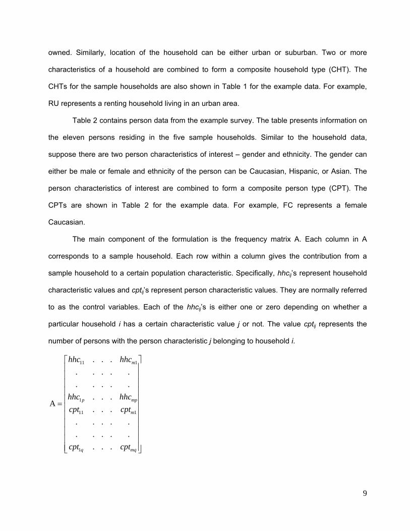
The main component of the formulation is the frequency matrix A. Each column in A

corresponds to a sample household. Each row within a column gives the contribution from a

sample household to a certain population characteristic. Specifically, hhcij’s represent household

characteristic values and cptij’s represent person characteristic values. They are normally referred

to as the control variables. Each of the hhcij’s is either one or zero depending on whether a

particular household i has a certain characteristic value j or not. The value cptij represents the

number of persons with the person characteristic j belonging to household i.

⎥⎥⎥⎥⎥⎥⎥⎥⎥⎥⎥

⎦

⎤

⎢⎢⎢⎢⎢⎢⎢⎢⎢⎢⎢

⎣

⎡

=

mqq

m

mpp

m

cptcpt

cptcpthhchhc

hhchhc

.............

...

.............

...

A

1

111

1

111

10

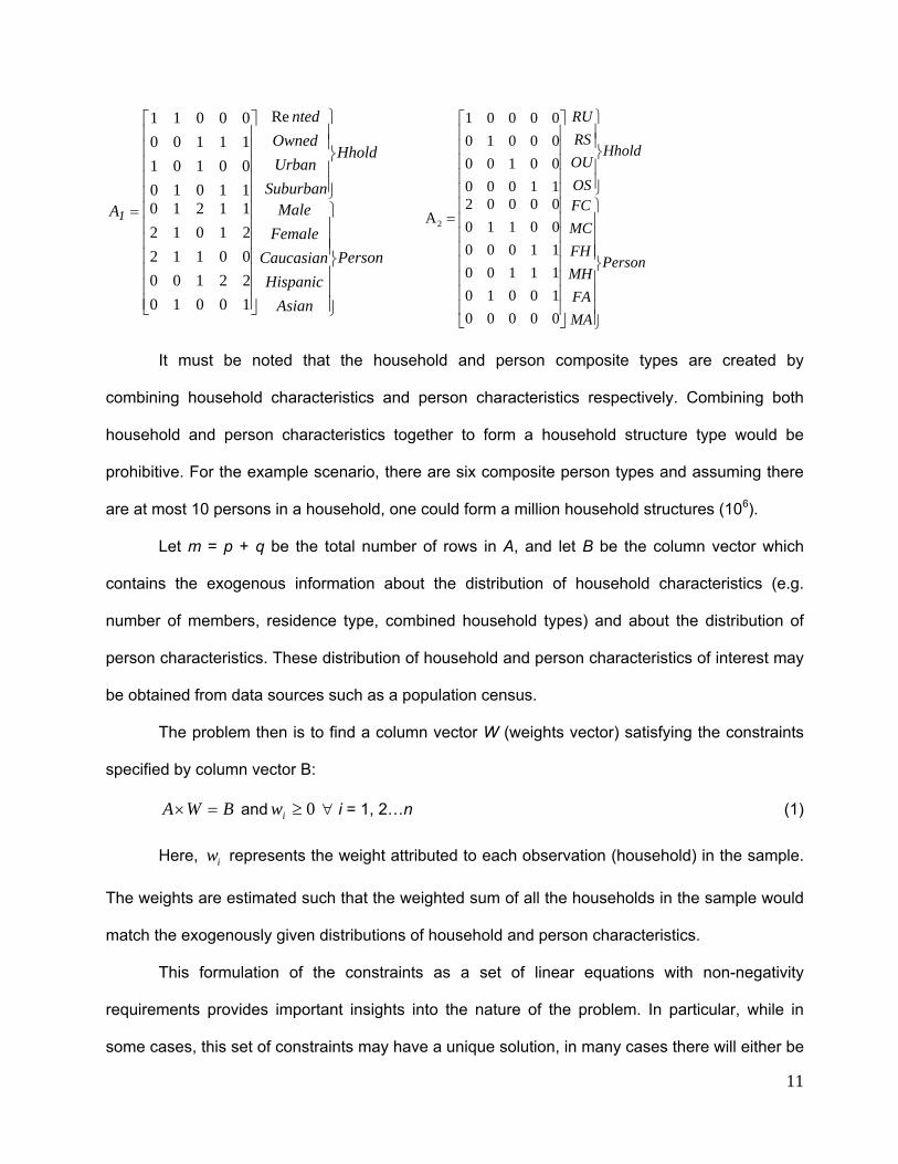
The construction of matrix A is illustrated with the help of the hypothetical survey data

presented in Tables 1 and 2. If only marginal totals by each population (household and person)

characteristic are separately available, then matrix A1 is constructed. Consider information about

household 3 (column 3 of matrix A1). The house is owned, therefore the element corresponding to

the ‘rented’ row is 0 and that corresponding to the ‘owned’ row is 1. The house is located in an

urban area, so the element corresponding to the ‘suburban’ row is 0 and that corresponding to

the ‘urban’ row is 1. There are two males in the household (from Table 2). One is Caucasian and

the other is Hispanic. Therefore, the elements corresponding to the rows ‘Male’, ‘Caucasian’ and

‘Hispanic’ are two, one and one respectively. All the other elements in the third column are

zeroes.

On the other hand, if the frequency distribution for the composite household and person

types obtained by combining more than one population characteristic is available then matrix A2

is constructed. Considering household 3 again, we will illustrate the construction of A2 matrix.

Since it is an owned house and located in an urban area, the element corresponding to the

composite row ‘OU’ row is 1 and the elements corresponding to other household types ‘RU’, ‘RS’

and ‘OS’ will be 0. Out of the two persons belonging to the household, one is a Caucasian male

and the other is a Hispanic male. Therefore, the elements corresponding to the rows ‘MC’ and

‘MH’ are 1 and 1 respectively. Note that in the composite type representation, there may be more

than one person of the same type in the household. For example there are two Caucasian

females in household 1 and the element corresponding to ‘FC’ under column of household 1 will

be equal to 2. The possibility of values above 1 in matrix A highlights one of the main differences

between travel surveys and other surveys.

11

Person

AsianHispanic

CaucasianFemaleMale

Hhold

SuburbanUrbanOwned

nted

A1

⎪⎪⎪

⎭

⎪⎪⎪

⎬

⎫

⎪⎪⎭

⎪⎪⎬

⎫

⎥⎥⎥⎥⎥⎥⎥⎥⎥⎥⎥⎥

⎦

⎤

⎢⎢⎢⎢⎢⎢⎢⎢⎢⎢⎢⎢

⎣

⎡

=

Re

100102210000112210121121011010001011110000011

Person

MAFAMHFHMCFC

Hhold

OSOURSRU

⎪⎪⎪⎪

⎭

⎪⎪⎪⎪

⎬

⎫

⎪⎪⎭

⎪⎪⎬

⎫

⎥⎥⎥⎥⎥⎥⎥⎥⎥⎥⎥⎥⎥

⎦

⎤

⎢⎢⎢⎢⎢⎢⎢⎢⎢⎢⎢⎢⎢

⎣

⎡

=

00000100101110011000001100000211000001000001000001

A2

It must be noted that the household and person composite types are created by

combining household characteristics and person characteristics respectively. Combining both

household and person characteristics together to form a household structure type would be

prohibitive. For the example scenario, there are six composite person types and assuming there

are at most 10 persons in a household, one could form a million household structures (106).

Let m = p + q be the total number of rows in A, and let B be the column vector which

contains the exogenous information about the distribution of household characteristics (e.g.

number of members, residence type, combined household types) and about the distribution of

person characteristics. These distribution of household and person characteristics of interest may

be obtained from data sources such as a population census.

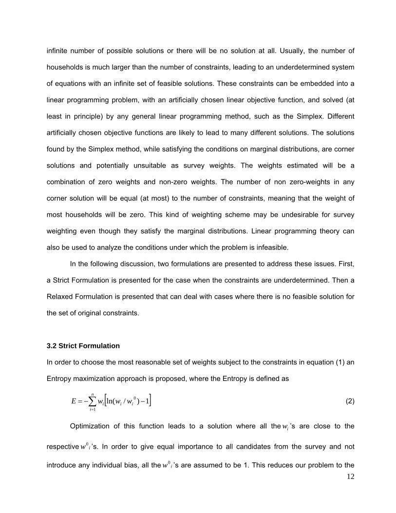
The problem then is to find a column vector W (weights vector) satisfying the constraints

specified by column vector B:

BWA =× and 0≥iw ∀ i = 1, 2…n (1)

Here, iw represents the weight attributed to each observation (household) in the sample.

The weights are estimated such that the weighted sum of all the households in the sample would

match the exogenously given distributions of household and person characteristics.

This formulation of the constraints as a set of linear equations with non-negativity

requirements provides important insights into the nature of the problem. In particular, while in

some cases, this set of constraints may have a unique solution, in many cases there will either be

12

infinite number of possible solutions or there will be no solution at all. Usually, the number of

households is much larger than the number of constraints, leading to an underdetermined system

of equations with an infinite set of feasible solutions. These constraints can be embedded into a

linear programming problem, with an artificially chosen linear objective function, and solved (at

least in principle) by any general linear programming method, such as the Simplex. Different

artificially chosen objective functions are likely to lead to many different solutions. The solutions

found by the Simplex method, while satisfying the conditions on marginal distributions, are corner

solutions and potentially unsuitable as survey weights. The weights estimated will be a

combination of zero weights and non-zero weights. The number of non zero-weights in any

corner solution will be equal (at most) to the number of constraints, meaning that the weight of

most households will be zero. This kind of weighting scheme may be undesirable for survey

weighting even though they satisfy the marginal distributions. Linear programming theory can

also be used to analyze the conditions under which the problem is infeasible.

In the following discussion, two formulations are presented to address these issues. First,

a Strict Formulation is presented for the case when the constraints are underdetermined. Then a

Relaxed Formulation is presented that can deal with cases where there is no feasible solution for

the set of original constraints.

3.2 Strict Formulation

In order to choose the most reasonable set of weights subject to the constraints in equation (1) an

Entropy maximization approach is proposed, where the Entropy is defined as

[ ]∑=

−−=n

iiii wwwE

1

0 1)/ln( (2)

Optimization of this function leads to a solution where all the iw ’s are close to the

respective iw0 ’s. In order to give equal importance to all candidates from the survey and not

introduce any individual bias, all the iw0 ’s are assumed to be 1. This reduces our problem to the

13

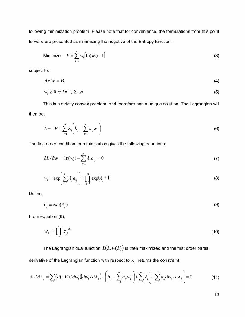
following minimization problem. Please note that for convenience, the formulations from this point

forward are presented as minimizing the negative of the Entropy function.

Minimize [ ]∑=

−=−n

iii wwE

11)ln( (3)

subject to:

BWA =× (4)

0≥iw ∀ i = 1, 2…n (5)

This is a strictly convex problem, and therefore has a unique solution. The Lagrangian will

then be,

∑ ∑= =

⎟⎠

⎞⎜⎝

⎛−+−=

m

j

n

iiijjj wabEL

1 1λ (6)

The first order condition for minimization gives the following equations:

0)ln(/1

=−=∂∂ ∑=

m

jijjii awwL λ (7)

( )∏∑==

=⎟⎟⎠

⎞⎜⎜⎝

⎛=

m

j

aj

m

jijji

ijaw11

expexp λλ (8)

Define,

)exp( jjc λ≡ (9)

From equation (8),

∏=

=m

j

aji

ijcw1

(10)

The Lagrangian dual function ( ))(, λλ wL is then maximized and the first order partial

derivative of the Lagrangian function with respect to jλ returns the constraint.

( )( ) 0///)(/1111

=⎟⎠

⎞⎜⎝

⎛∂∂−+⎟

⎠

⎞⎜⎝

⎛−+∂∂∂−∂=∂∂ ∑∑∑∑

====

n

ijiij

m

ll

n

iiijj

n

ijiij wawabwwEL λλλλ (11)

14

⎟⎟⎠

⎞⎜⎜⎝

⎛=∂∂ ∑

=

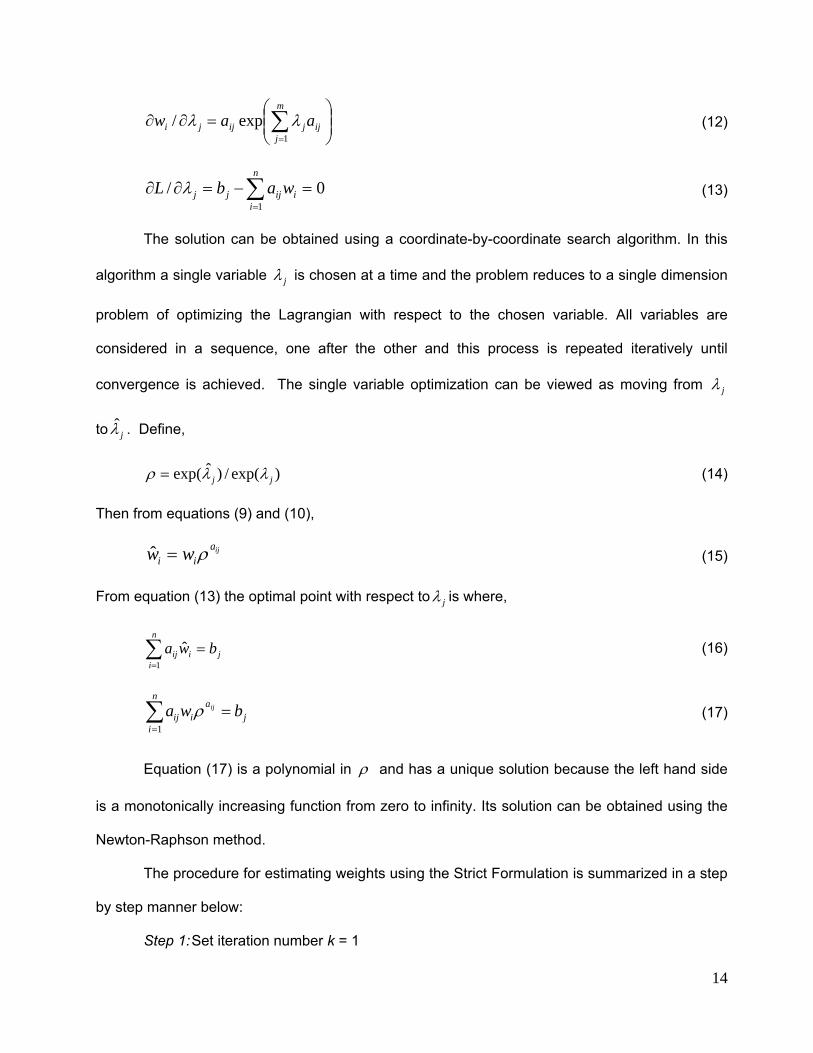
m

jijjijji aaw

1exp/ λλ (12)

0/1

=−=∂∂ ∑=

n

iiijjj wabL λ (13)

The solution can be obtained using a coordinate-by-coordinate search algorithm. In this

algorithm a single variable jλ is chosen at a time and the problem reduces to a single dimension

problem of optimizing the Lagrangian with respect to the chosen variable. All variables are

considered in a sequence, one after the other and this process is repeated iteratively until

convergence is achieved. The single variable optimization can be viewed as moving from jλ

to jλ̂ . Define,

)exp(/)ˆexp( jj λλρ = (14)

Then from equations (9) and (10),

ijaii ww ρ=ˆ (15)

From equation (13) the optimal point with respect to jλ is where,

j

n

iiij bwa =∑

=1

ˆ (16)

j

n

i

aiij bwa ij =∑

=1

ρ (17)

Equation (17) is a polynomial in ρ and has a unique solution because the left hand side

is a monotonically increasing function from zero to infinity. Its solution can be obtained using the

Newton-Raphson method.

The procedure for estimating weights using the Strict Formulation is summarized in a step

by step manner below:

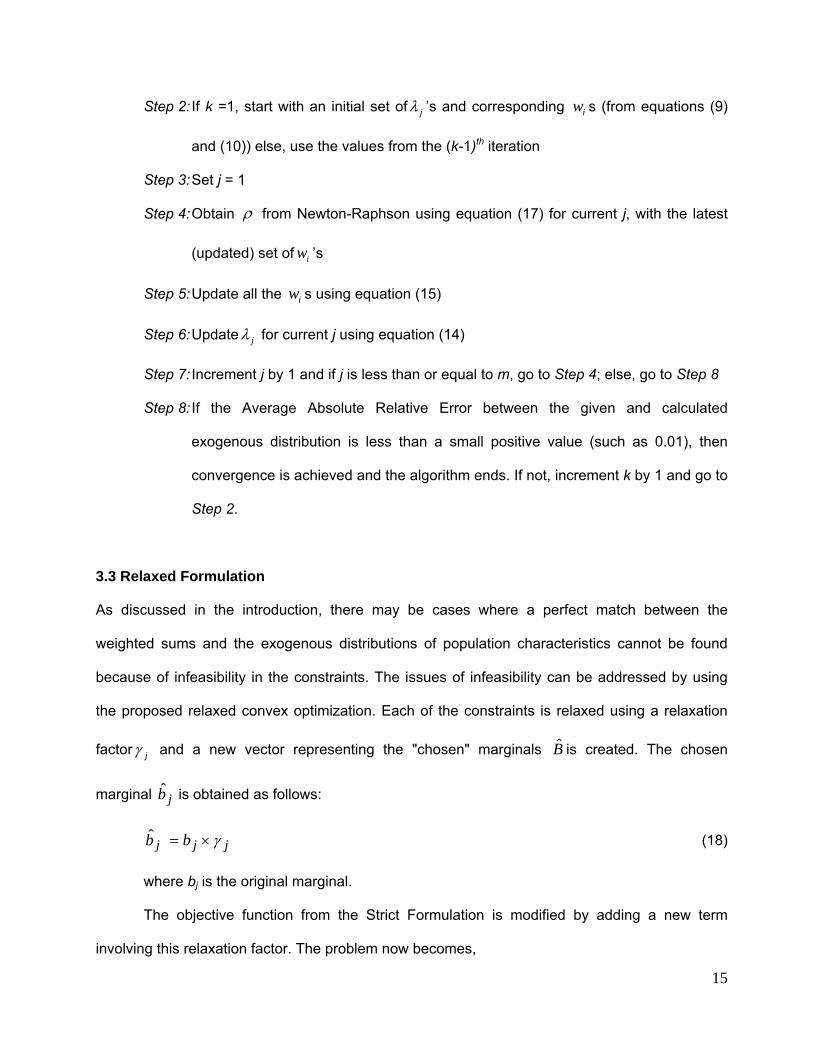
Step 1: Set iteration number k = 1

15

Step 2: If k =1, start with an initial set of jλ ’s and corresponding iw s (from equations (9)

and (10)) else, use the values from the (k-1)th iteration

Step 3: Set j = 1

Step 4: Obtain ρ from Newton-Raphson using equation (17) for current j, with the latest

(updated) set of iw ’s

Step 5: Update all the iw s using equation (15)

Step 6: Update jλ for current j using equation (14)

Step 7: Increment j by 1 and if j is less than or equal to m, go to Step 4; else, go to Step 8

Step 8: If the Average Absolute Relative Error between the given and calculated

exogenous distribution is less than a small positive value (such as 0.01), then

convergence is achieved and the algorithm ends. If not, increment k by 1 and go to

Step 2.

3.3 Relaxed Formulation

As discussed in the introduction, there may be cases where a perfect match between the

weighted sums and the exogenous distributions of population characteristics cannot be found

because of infeasibility in the constraints. The issues of infeasibility can be addressed by using

the proposed relaxed convex optimization. Each of the constraints is relaxed using a relaxation

factor jγ and a new vector representing the "chosen" marginals B̂ is created. The chosen

marginal j b̂ is obtained as follows:

jjj bb γ×=ˆ (18)

where bj is the original marginal.

The objective function from the Strict Formulation is modified by adding a new term

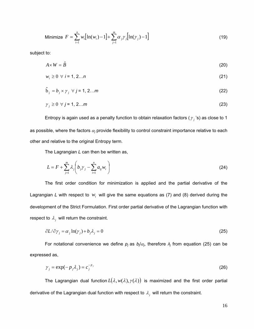
involving this relaxation factor. The problem now becomes,

16

Minimize [ ] [ ]∑∑==

−+−=m

jjjj

n

iii wwF

111)ln(1)ln( γγα (19)

subject to:

BWA ˆ=× (20)

0≥iw ∀ i = 1, 2…n (21)

jjb γ×= jb̂ ∀ j = 1, 2…m (22)

0≥jγ ∀ j = 1, 2…m (23)

Entropy is again used as a penalty function to obtain relaxation factors ( jγ ’s) as close to 1

as possible, where the factors αj provide flexibility to control constraint importance relative to each

other and relative to the original Entropy term.

The Lagrangian L can then be written as,

∑ ∑= =

⎟⎠

⎞⎜⎝

⎛−+=

m

j

n

iiijjjj wabFL

1 1γλ (24)

The first order condition for minimization is applied and the partial derivative of the

Lagrangian L with respect to iw will give the same equations as (7) and (8) derived during the

development of the Strict Formulation. First order partial derivative of the Lagrangian function with

respect to jλ will return the constraint.

0)ln(/ =+=∂∂ jjjjj bL λγαγ (25)

For notational convenience we define pj as bj/αj, therefore λj from equation (25) can be

expressed as,

jpjjjj cp −=−= )exp( λγ (26)

The Lagrangian dual function ( ))(),(, λγλλ wL is maximized and the first order partial

derivative of the Lagrangian dual function with respect to jλ will return the constraint.

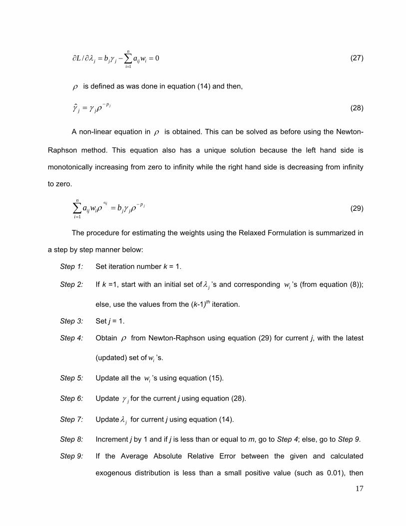
17

0/1

=−=∂∂ ∑=

n

iiijjjj wabL γλ (27)

ρ is defined as was done in equation (14) and then,

jpjj

−= ργγ̂ (28)

A non-linear equation in ρ is obtained. This can be solved as before using the Newton-

Raphson method. This equation also has a unique solution because the left hand side is

monotonically increasing from zero to infinity while the right hand side is decreasing from infinity

to zero.

jija p

jj

n

iiij bwa −

=

=∑ ργρ1

(29)

The procedure for estimating the weights using the Relaxed Formulation is summarized in

a step by step manner below:

Step 1: Set iteration number k = 1.

Step 2: If k =1, start with an initial set of jλ ’s and corresponding iw ’s (from equation (8));

else, use the values from the (k-1)th iteration.

Step 3: Set j = 1.

Step 4: Obtain ρ from Newton-Raphson using equation (29) for current j, with the latest

(updated) set of iw ’s.

Step 5: Update all the iw ’s using equation (15).

Step 6: Update jγ for the current j using equation (28).

Step 7: Update jλ for current j using equation (14).

Step 8: Increment j by 1 and if j is less than or equal to m, go to Step 4; else, go to Step 9.

Step 9: If the Average Absolute Relative Error between the given and calculated

exogenous distribution is less than a small positive value (such as 0.01), then

18

convergence criterion is met and algorithm ends. If not, increment k by 1 and go to

Step 2.

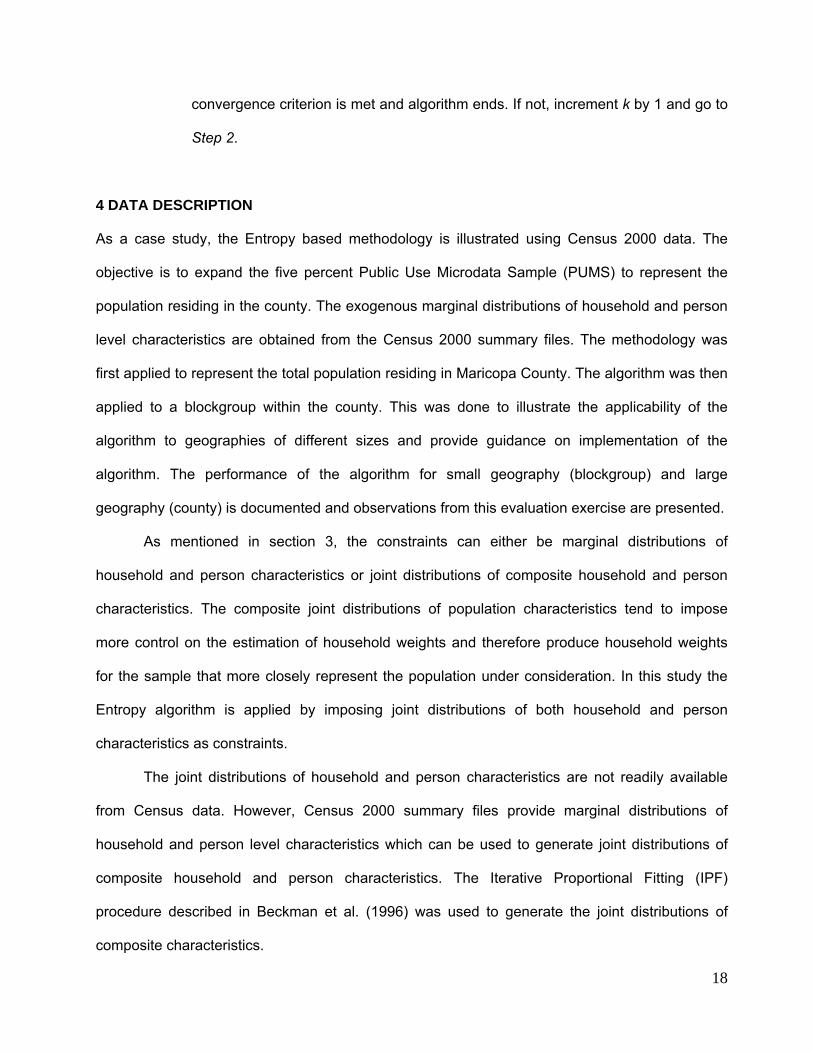
4 DATA DESCRIPTION

As a case study, the Entropy based methodology is illustrated using Census 2000 data. The

objective is to expand the five percent Public Use Microdata Sample (PUMS) to represent the

population residing in the county. The exogenous marginal distributions of household and person

level characteristics are obtained from the Census 2000 summary files. The methodology was

first applied to represent the total population residing in Maricopa County. The algorithm was then

applied to a blockgroup within the county. This was done to illustrate the applicability of the

algorithm to geographies of different sizes and provide guidance on implementation of the

algorithm. The performance of the algorithm for small geography (blockgroup) and large

geography (county) is documented and observations from this evaluation exercise are presented.

As mentioned in section 3, the constraints can either be marginal distributions of

household and person characteristics or joint distributions of composite household and person

characteristics. The composite joint distributions of population characteristics tend to impose

more control on the estimation of household weights and therefore produce household weights

for the sample that more closely represent the population under consideration. In this study the

Entropy algorithm is applied by imposing joint distributions of both household and person

characteristics as constraints.

The joint distributions of household and person characteristics are not readily available

from Census data. However, Census 2000 summary files provide marginal distributions of

household and person level characteristics which can be used to generate joint distributions of

composite household and person characteristics. The Iterative Proportional Fitting (IPF)

procedure described in Beckman et al. (1996) was used to generate the joint distributions of

composite characteristics.

19

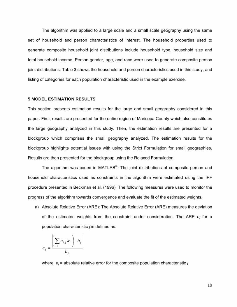
The algorithm was applied to a large scale and a small scale geography using the same

set of household and person characteristics of interest. The household properties used to

generate composite household joint distributions include household type, household size and

total household income. Person gender, age, and race were used to generate composite person

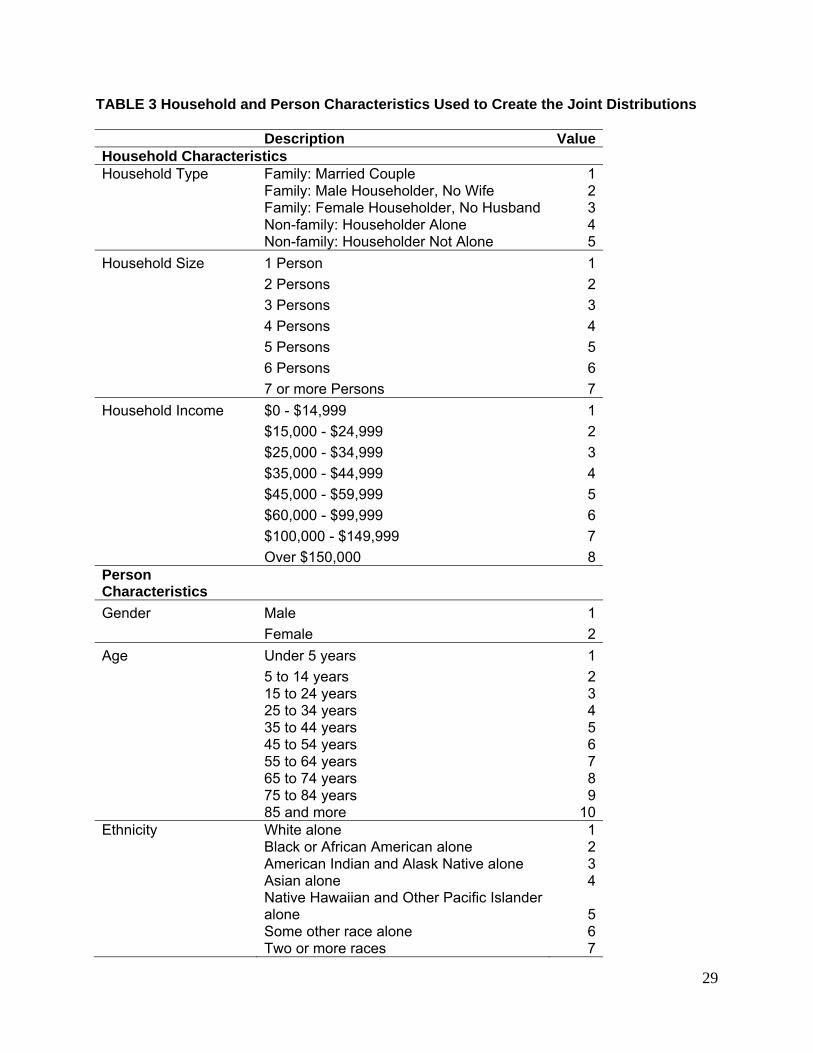
joint distributions. Table 3 shows the household and person characteristics used in this study, and

listing of categories for each population characteristic used in the example exercise.

5 MODEL ESTIMATION RESULTS

This section presents estimation results for the large and small geography considered in this

paper. First, results are presented for the entire region of Maricopa County which also constitutes

the large geography analyzed in this study. Then, the estimation results are presented for a

blockgroup which comprises the small geography analyzed. The estimation results for the

blockgroup highlights potential issues with using the Strict Formulation for small geographies.

Results are then presented for the blockgroup using the Relaxed Formulation.

The algorithm was coded in MATLAB®. The joint distributions of composite person and

household characteristics used as constraints in the algorithm were estimated using the IPF

procedure presented in Beckman et al. (1996). The following measures were used to monitor the

progress of the algorithm towards convergence and evaluate the fit of the estimated weights.

a) Absolute Relative Error (ARE): The Absolute Relative Error (ARE) measures the deviation

of the estimated weights from the constraint under consideration. The ARE ej for a

population characteristic j is defined as:

j

ji

iji

j b

bwae

−⎟⎠

⎞⎜⎝

⎛

=∑ ,

where ej = absolute relative error for the composite population characteristic j

20

ai,j = value of element in matrix A corresponding to sample point i and population

characteristic j

bj = value of the population characteristic j from the marginal distribution

wi = weight attributed to sample point i from the previous iteration

In an ideal situation, when the household weights perfectly match the population

distributions, the ARE value is zero for all population characteristics. The Maximum

Absolute Relative Error (MARE) is the maximum of ARE for all population characteristics.

In this study, the progress of the algorithm was monitored using the MARE. A value of

MARE close to zero indicates convergence of the algorithm for a particular geography.

Although the ARE is a very good measure for monitoring convergence, it can sometimes

be misleading. For example a value of ARE equal to 1 may be obtained when the

estimate is 0 and the control is 0.2, and also when the estimated value is 200 and the

control value is 100. It can easily be seen that, the difference in the first example may be

reasonable, but it may not be acceptable in the second example. Therefore, although the

ARE was used to monitor the progress of the algorithm, it was not used to compare the

estimated population characteristic distributions against those obtained from the IPF

procedure.

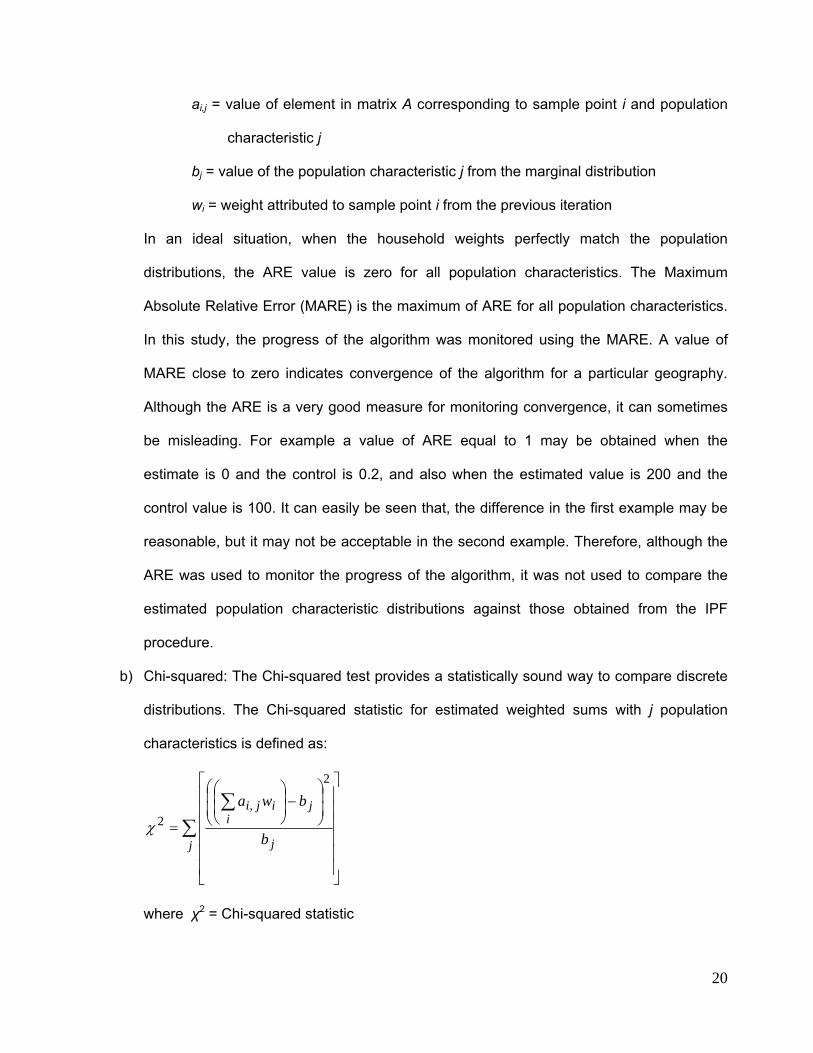
b) Chi-squared: The Chi-squared test provides a statistically sound way to compare discrete

distributions. The Chi-squared statistic for estimated weighted sums with j population

characteristics is defined as:

∑∑

⎥⎥⎥⎥⎥⎥

⎦

⎤

⎢⎢⎢⎢⎢⎢

⎣

⎡

⎟⎟⎠

⎞⎜⎜⎝

⎛−⎟

⎟⎠

⎞⎜⎜⎝

⎛

=j j

ji

iji

b

bwa2

,2χ

where χ2 = Chi-squared statistic

21

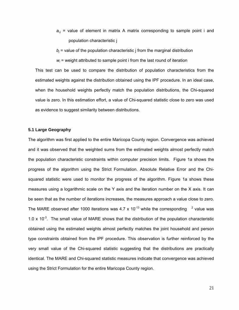
ai,j = value of element in matrix A matrix corresponding to sample point i and

population characteristic j

bj = value of the population characteristic j from the marginal distribution

wi = weight attributed to sample point i from the last round of iteration

This test can be used to compare the distribution of population characteristics from the

estimated weights against the distribution obtained using the IPF procedure. In an ideal case,

when the household weights perfectly match the population distributions, the Chi-squared

value is zero. In this estimation effort, a value of Chi-squared statistic close to zero was used

as evidence to suggest similarity between distributions.

5.1 Large Geography

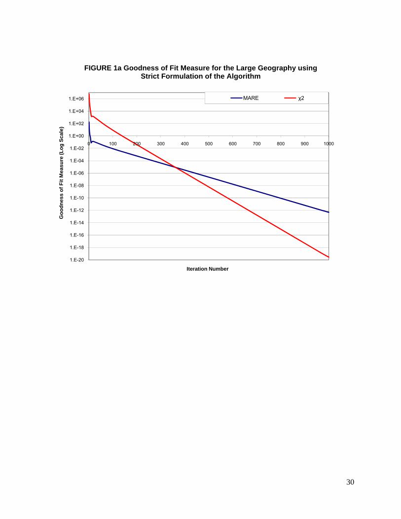
The algorithm was first applied to the entire Maricopa County region. Convergence was achieved

and it was observed that the weighted sums from the estimated weights almost perfectly match

the population characteristic constraints within computer precision limits. Figure 1a shows the

progress of the algorithm using the Strict Formulation. Absolute Relative Error and the Chi-

squared statistic were used to monitor the progress of the algorithm. Figure 1a shows these

measures using a logarithmic scale on the Y axis and the iteration number on the X axis. It can

be seen that as the number of iterations increases, the measures approach a value close to zero.

The MARE observed after 1000 iterations was 4.7 x 10-13 while the corresponding �2 value was

1.0 x 10-3. The small value of MARE shows that the distribution of the population characteristic

obtained using the estimated weights almost perfectly matches the joint household and person

type constraints obtained from the IPF procedure. This observation is further reinforced by the

very small value of the Chi-squared statistic suggesting that the distributions are practically

identical. The MARE and Chi-squared statistic measures indicate that convergence was achieved

using the Strict Formulation for the entire Maricopa County region.

22

5.2 Small Geography

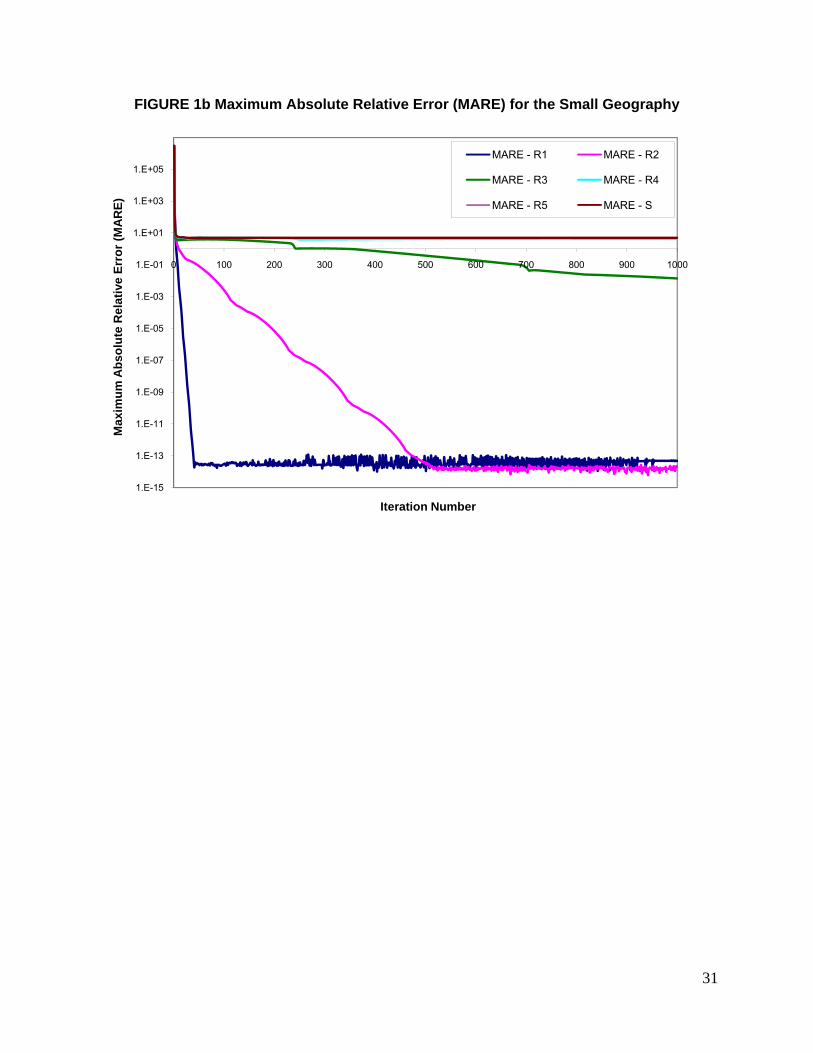
The lines represented by S in Figures 1b and 1c show the progress of the algorithm using the

Strict Formulation for the blockgroup. The MARE and Chi-squared statistic measures in the

figures are shown on the Y axis using a logarithmic scale and the iteration number is shown on

the X axis. It can be seen from the figures that the curve representing the MARE plateaus after 60

iterations and remains at a value of about 5.04. The Chi-squared statistic also plateaus after

about 60 iterations and decreases at a very slow rate. After 1000 iterations, the MARE observed

for the Strict Formulation was about 5.04 and the Chi-Squared value observed was about 13.81.

The high value of MARE suggests that there is at least one population characteristic whose

constraint was not satisfied, in other words a solution was not found. As discussed earlier, this is

caused when the given joint household and person type constraints are infeasible.

In this particular example we were actually able to verify that the problem is infeasible due

to contradiction in the original constraints. The results from the IPF procedure provide a target

total weighted sum of 0.0752 for ‘seven person non-family households in the lowest income level’

category. There are only two households in the survey belonging to this composite type. In one of

these households, there are six males 15-24 years old belonging to ethnicity category 6. The

target total for this composite person type is 0.0214, hence the maximum possible weight for the

first household is 0.0036. In the second household, there are two females 5-14 years old in the

sixth ethnicity category. The target total for this composite person type is 0.0021. Hence the

maximum possible weight for the second household is 0.001. In total the sum of the weights of

the two households in this composite household type cannot exceed 0.0046, about 16 times

lower than the target total. Clearly it is not possible to satisfy these three conditions

simultaneously with the given sample of households.

A possible resolution is to use the Relaxed Formulation. Figures 1b and 1c plot the MARE

and Chi-squared statistic for the Relaxed Formulation using different levels of Relaxation (R1, R2,

R3, R4, R5). The Relaxation levels R1, R2, R3, R4, and R5 were achieved by maintaining pj from

23

equation (26) at 1.0, 0.1, 0.01, 0.001, 0.0001 respectively for both person and household

constraints. Relaxation R1 corresponds to the most relaxed case and R5 corresponds to the least

relaxed case. The results from R5 are very similar to the strict formulation results because of the

very little amount of relaxation allowed by the corresponding pj value.

It can be seen from Figure 1b that with relaxation, the value of MARE has decreased

when compared to the Strict Formulation. The change in the value of MARE decreases with

increase in level of relaxation. The change in the value of MARE is greater for Relaxation R1

compared to that of Relaxation R5 which almost overlaps the curve traced by the Strict

Formulation. The figure also shows that convergence was achieved for the Relaxed Formulation

for cases R1, R2, and R3 while the cases R4 and R5 exhibit behavior similar to the Strict

Formulation. It should be noted that convergence in the Relaxed Formulation comes at the price

of altering the constraints; as a result the distribution of population characteristics obtained from

the algorithm are further away from the target distributions. The MARE calculated in the Relaxed

Formulation is with respect to the relaxed constraints and not using the constraints from the IPF

procedure. Therefore the MARE for the Relaxed Formulation only provides a way to monitor the

progress of the algorithm and should not be used to measure the goodness of fit. Goodness of fit

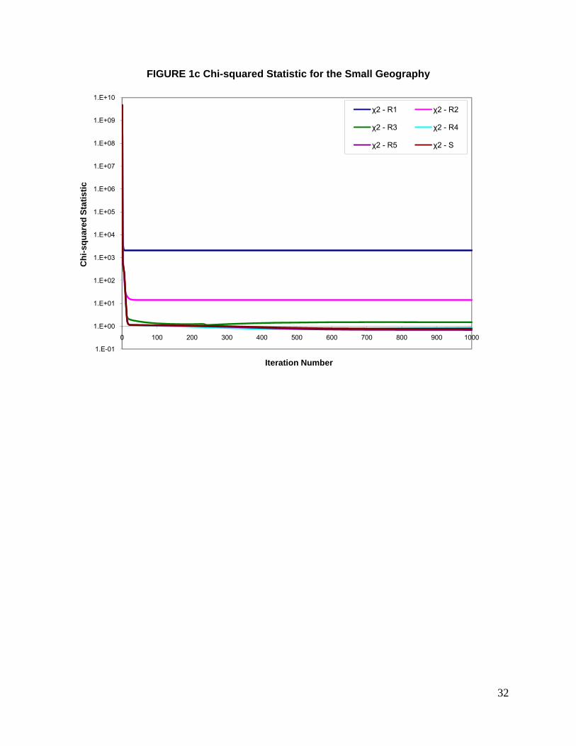
under the Relaxed Formulation can be evaluated using the Chi-squared statistic. Figure 1c shows

that the Chi-squared value does not improve a lot with relaxation, especially for cases with

Relaxation R1 and R2. This is expected because, when the constraints are relaxed, one is

moving away from the objective constraints; as a result, the Chi-squared statistic is larger

compared to the Strict Formulation. With relaxation R3 and R4, Chi-squared statistics of 0.74 and

0.26 were estimated showing a marginal improvement in fit with relaxation. It is interesting to note

that for Relaxation R5 the Chi-squared value is very similar to that of the Strict Formulation

indicating that very small relaxations may not contribute much towards convergence and also

there is no loss in the goodness of fit. Alternate formulations for relaxation of constraints can

further improve the fit and is a good candidate for further research in the area.

24

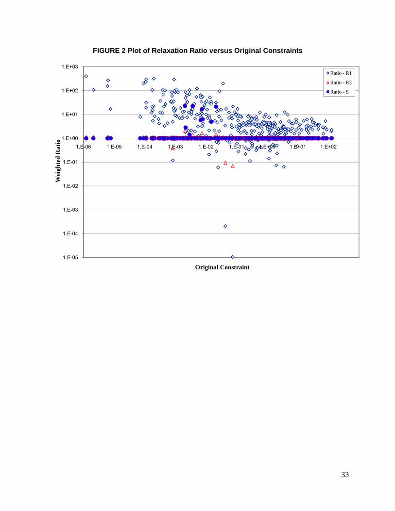
Figure 2 shows the scatter plots for Relaxation R1, R3 and S with weighted ratio on the Y

axis and the original constraint on the X axis. Weighted ratio is defined as the ratio of the

weighted sum for the population characteristic to that of the original constraint. The values on

both X and Y axes are plotted using a logarithmic scale. The scatter plots shown in the figure

correspond to three levels of relaxation where R1 corresponds to highest relaxation, R3

corresponds to moderate relaxation and Strict Formulation corresponds to no relaxation. It was

observed that the weighted ratios for the Relaxation R3 are close to the Strict Formulation while

that for Relaxation R1 are very different. It can be seen that weighted ratios are larger for smaller

values of original constraints. On the other hand, the weighted ratios are smaller for original

constraints with higher magnitude. It was also observed that the weighted ratios for relaxation R1

varied from 1.04 x 10-5 to 400.23, for relaxation R3 the variation was between 0.07 and 2.09, and

finally for the strict formulation the variation was from 1.00 to 22.74. The ranges of weighted ratios

corroborate our earlier observation showing slight improvement in the Chi-squared statistic with

Relaxation levels R3 and R4.

It can therefore be seen that the Relaxed Formulation can be used to estimate weights

when the constraints are infeasible and still be able satisfy the population characteristic

constraints to within reasonable limits. The choice of level of relaxation needs further exploration

and is another good candidate for research in the area.

6 CONCLUSIONS

Transportation professionals are often faced with the challenge of accurately expanding the

survey households to represent the population. The problem becomes even more complicated

when dealing with household travel surveys, because the goal is to find household weights such

that the distributions of the population characteristics from the estimated weights should not only

match given distributions of households but also that of persons. An Entropy Maximization

25

methodology is presented in this paper that can not only match the exogenously given

distributions of the households but also the person distributions.

The model estimation results provide valuable insights into the actual formulation and the

accuracy of the household weights for different extents of geography. The Strict Formulation

presented in this paper can be used to estimate weights when the constraints are feasible. The

resulting weighted sums almost perfectly match the distributions of the population characteristics.

Therefore, Strict Formulation is appropriate for geographies with larger extents where the

constraints are generally feasible. On the other hand, smaller geographies are more likely to

suffer from infeasible constraints. In the case we examined, the results of the strict formulation

may be acceptable. Additional flexibility can be obtained by the relaxed formulation as was

observed with moderate relaxation levels. Additional research is needed to evaluate the potential

advantages of this flexibility, and particularly to study the relationship between the level of

relaxation, level of fit and the computation time.

7 REFERENCES

Akamatsu T (1997) Decomposition of Path Choice Entropy in General Transport Networks.

Transportation Science 31(4): 349-362.

Alexander CH and Roebuck MJ (1986) Comparison of Alternative Methods for Household

Estimation. American Statistical Association Proceedings of the Section on the Survey

Research Methods: 64-71.

Asiala ME (2007) Weighting and Estimation Research Methodology and Results From the

American Community Survey Family Equalization Project. Federal Committee on

Statistical Methodology Research Conference.

Beckman RJ, Baggerly KA & McKay MD (1996) Creating Synthetic Baseline Populations.

Transportation Research Part A 30(6): 415-429.

26

Daganzo, CF & Sheffi Y (1977) On Stochastic Models of Traffic Assignment. Transportation

Science 11: 253-274.

Deming WE & Stephan FF (1940) On a Least Squares Adjustment of Sampled Frequency Table

When the Expected Marginal Totals are Known. The Annals of Mathematical Statistics

11(4): 427-444.

Dial RB (1971) A probabilistic Multipath Traffic Assignment Algorithm which Obviates Path

Enumeration. Transportation Research 5: 83-111.

Fang SC, & Tsao H-SJ (1995) Linearly-Constrained Entropy Maximization Problem with

Quadratic Cost and Its Applications to Transportation Planning Problems. Transportation

Science 29(4): 353-365

Feinberg SE (1970) An Iterative Procedure for Estimation in Contingency Tables. The Annals of

Mathematical Statistics 47(3): 907-917.

Harrington I & Wang C-Y (1995) Adjusting Household Survey Expansion Factors. Fifth National

Conference on Transportation Planning Methods Applications -Volume II.

Harrington I & Wang C-Y (1995) Modifying Transit Mode Share in Household Survey Expansion.

Transportation Research Record 1496: 25-34.

Ireland CT & Kullback S (1968) Contingency Tables with Given Marginals. Biometrika 55(1): 179-

188.

Jornsten KO & Lundgren JT (1989) An Entropy-Based Modal Split Model. Transportation

Research Part B 23(5): 345-349.

Li Y, Ziliaskopoulos T & Boyce, D (2002) Combined Model for Time-dependent Trip Distribution

and Traffic Assignment. Transportation Research Record 1783: 98-110.

Oppenheim N (1995) Urban Travel Demand Modeling: From Individual Choices to General

Equilibrium. Wiley-Interscience Publication.

Rossi TF, McNeil S & Hendrickson C (1989) Entropy Model for Consistent Impact Fee

Assessment. Journal of Urban Planning and Development 115(2): 51-63.

27

Sheffi Y (1985) Urban Transportation Networks: Equilibrium Analysis with Mathematical

Programming Methods. Prentice Hall, Englewood Cliffs.

Stopher PR & Metcalf HMA (1996) Methods for Household Travel Surveys. NCHRP

Synthesis of Highway Practice 236, Transportation Research Board, Washington D.C.

Wang D, Yao R & Jing C (2006) Entropy Models of Trip Distribution. Journal of Urban Planning

and Development 132(1): 29-35.

Wilson AG (1967) A Statistical Theory of Spatial Distribution Models. Transportation Resrearch

1(3).

Wilson AG (1969) The Use of Entropy Maximizing Models in the Theory of Trip Distribution, Mode

Split and Route Split. Journal of Transport Economics and Policy 3: 108-126.

Wilson AG (1970) The Use of the Concept of Entropy in System Modelling. Operational Research

Quarterly 21(2): 247-265.

TABLE 1 Household Data for the Sample Survey

Household Index Ownership R - Rent, O - Own

Location U - Urban,

S - Suburban

Composite Household Type

1 R U RU 2 R S RS 3 O U OU 4 O S OS 5 O S OS

TABLE 2 Person Data for the Sample Survey

Household Index

Person Index

Gender M - Male,

F - Female

Ethnicity C - Caucasian, H - Hispanic,

A - Asian

Composite Person Type

1 1 F C FC 1 2 F C FC 2 1 M C MC 2 2 F A FA 3 1 M H MH 3 2 M C MC 4 1 F H FH 4 2 M H MH 5 1 M H MH 5 2 F A FA 5 3 F H FH

29

TABLE 3 Household and Person Characteristics Used to Create the Joint Distributions Description Value Household Characteristics Household Type Family: Married Couple 1 Family: Male Householder, No Wife 2 Family: Female Householder, No Husband 3 Non-family: Householder Alone 4 Non-family: Householder Not Alone 5 Household Size 1 Person 1 2 Persons 2 3 Persons 3 4 Persons 4 5 Persons 5 6 Persons 6 7 or more Persons 7 Household Income $0 - $14,999 1 $15,000 - $24,999 2 $25,000 - $34,999 3 $35,000 - $44,999 4 $45,000 - $59,999 5 $60,000 - $99,999 6 $100,000 - $149,999 7 Over $150,000 8 Person Characteristics Gender Male 1 Female 2 Age Under 5 years 1 5 to 14 years 2 15 to 24 years 3 25 to 34 years 4 35 to 44 years 5 45 to 54 years 6 55 to 64 years 7 65 to 74 years 8 75 to 84 years 9 85 and more 10 Ethnicity White alone 1 Black or African American alone 2 American Indian and Alask Native alone 3 Asian alone 4

Native Hawaiian and Other Pacific Islander alone 5

Some other race alone 6 Two or more races 7

30

FIGURE 1a Goodness of Fit Measure for the Large Geography using Strict Formulation of the Algorithm

1.E-20

1.E-18

1.E-16

1.E-14

1.E-12

1.E-10

1.E-08

1.E-06

1.E-04

1.E-02

1.E+00

1.E+02

1.E+04

1.E+06

0 100 200 300 400 500 600 700 800 900 1000

Goo

dnes

s of

Fit

Mea

sure

(Log

Sca

le)

Iteration Number

MARE χ2

31

FIGURE 1b Maximum Absolute Relative Error (MARE) for the Small Geography

1.E-15

1.E-13

1.E-11

1.E-09

1.E-07

1.E-05

1.E-03

1.E-01

1.E+01

1.E+03

1.E+05

0 100 200 300 400 500 600 700 800 900 1000

Max

imum

Abs

olut

e R

elat

ive

Erro

r (M

AR

E)

Iteration Number

MARE - R1 MARE - R2

MARE - R3 MARE - R4

MARE - R5 MARE - S

32

FIGURE 1c Chi-squared Statistic for the Small Geography

1.E-01

1.E+00

1.E+01

1.E+02

1.E+03

1.E+04

1.E+05

1.E+06

1.E+07

1.E+08

1.E+09

1.E+10

0 100 200 300 400 500 600 700 800 900 1000

Chi

-squ

ared

Sta

tistic

Iteration Number

χ2 - R1 χ2 - R2

χ2 - R3 χ2 - R4

χ2 - R5 χ2 - S

33

FIGURE 2 Plot of Relaxation Ratio versus Original Constraints

1.E-05

1.E-04

1.E-03

1.E-02

1.E-01

1.E+00

1.E+01

1.E+02

1.E+03

1.E-06 1.E-05 1.E-04 1.E-03 1.E-02 1.E-01 1.E+00 1.E+01 1.E+02

Wei

ghte

d R

atio

Original Constraint

Ratio - R1

Ratio - R3

Ratio - S