Estimating Shadows with the Bright Channel Cue

Estimating Shadows with the BrightChannel Cue

Alexandros Panagopoulos1, Chaohui Wang2,3, Dimitris Samaras1 and NikosParagios2,3

1Image Analysis Lab, Computer Science Dept., Stony Brook University, NY, USA2Laboratoire MAS, Ecole Centrale Paris, Chatenay-Malabry, France

3Equipe GALEN, INRIA Saclay - Ile-de-France, Orsay, France

Abstract. In this paper, we introduce a simple but efficient cue for theextraction of shadows from a single color image, the bright channel cue.We discuss its limitations and offer two methods to refine the brightchannel: by computing confidence values for the cast shadows, based ona shadow-dependent feature, such as hue; and by combining the brightchannel with illumination invariant representations of the original imagein a flexible way using an MRF model. We present qualitative and quan-titative results for shadow detection, as well as results in illuminationestimation from shadows. Our results show that our method achievessatisfying results despite the simplicity of the approach.

1 Introduction

Shadows are an important visual cue in natural images. In many applicationsthey pose an additional challenge, complicating tasks such as object recognition.On the other hand, they provide information about the size and shape of theobjects, their relative positions, as well as about the light sources in the scene.It is however difficult to take advantage of the information provided by shad-ows in natural images, since it is hard to differentiate between shadows, albedovariations and other effects.

The detection of cast shadows in the general case is not straightforward.Shadow detection, in the absence of illumination estimation or knowledge of 3Dgeometry is a well studied problem. [1] uses invariant color features to segmentcast shadows in still or moving images. [2] suggests a method to detect andremove shadows based on the properties of shadow boundaries in the image. In[3, 4], a set of illumination invariant features is proposed to detect and removeshadows from a single image. This method is suited to images with relativelysharp shadows and makes some assumptions about the lights and the camera.Camera calibration is necessary; if this is not possible, an entropy minimizationmethod is proposed to recover the most probable illumination invariant image.In [5], a method for high-quality shadow detection and removal is discussed. Themethod, however, needs some very limited user input. Recently, [6] proposed amethod to detect shadows in the case of monochromatic images, based on aseries of features that capture statistical properties of the shadows.

2 A. Panagopoulos, C. Wang, D. Samaras, N. Paragios

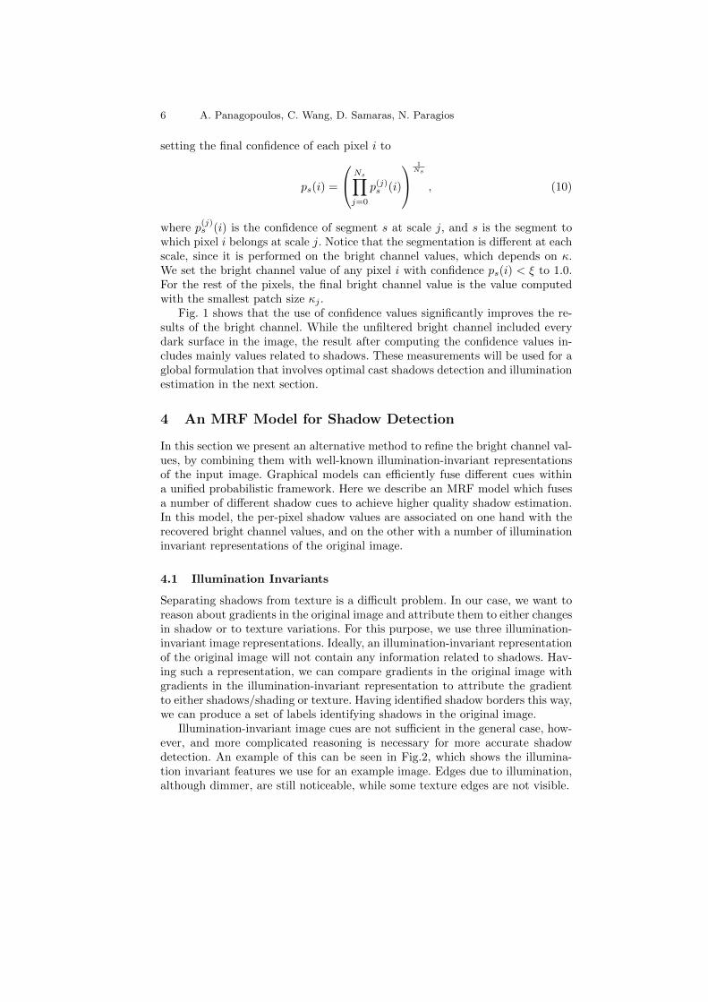
Fig. 1. Bright channel: a. original image (from [3]); b. bright channel; c. hue histogram;d. confidence map; e. refined bright channel; f. confidence computation: for a borderpixel i of segment s, we compare the two patches oriented along the image gradient

In this paper, we discuss the estimation of cast shadows in a scene from asingle color image.

We first propose a simple but effective image cue for the extraction of shad-ows, the bright channel, inspired from the dark channel prior [7]. Such a cueexploits the assumption that the value of each color channel of a pixel is limitedby the incoming radiance, but there are pixels in an arbitrary image patch withvalues close to the upper limit for at least one color channel.

Then we describe a method to compute confidence values for the cast shad-ows in an image, in order to alleviate some inherent limitations of the brightchannel prior. We process the bright channel in multiple scales and combine theresults. We also present an alternative approach for refining the bright channelvalues, utilizing a Markov Random Field (MRF) model. The MRF model com-bines the initial bright channel values with a number of illumination-invariantrepresentations to generate a labeling of shadow pixels in the image.

We evaluate our method on the dataset described in [6] and measure theaccuracy of pixel classification. We also provide results for qualitative evaluationon other images, and demonstrate an example use of our results to performillumination estimation with a very simple voting procedure.

This paper is organized as follows: Sec. 2 introduces the bright channel cue;Sec. 3 presents a way to compute confidences for cast shadows and refine thebright channel; Sec. 4 describes an MRF model to combine the bright channelwith illumination-invariant cues for shadow estimation, followed by experimentalresults in Sec. 5. Sec. 6 concludes the paper.

2 Bright channel cue concept

To define the bright channel cue, we consider the following observations:

– The value of each of the color channels of the image has an upper limit whichdepends on the incoming radiance. This means that, if little light arrives atthe 3D point corresponding to a given pixel, then all color channels will havelow values.

– In most images, if we examine an arbitrary image patch, the albedo for atleast some of the pixels in the patch will probably have a high value in atleast one of the color channels.

Estimating Shadows with the Bright Channel Cue 3

From the above observations we expect that, given an image patch, the maximumvalue of the r, g, b color channels should be roughly proportional to the incomingradiance. Therefore, we define the bright channel, Ibright for image I in a waysimilar to the definition of the dark channel [7]:

Ibright(i) = maxc∈r,g,b(maxj∈Ω(i)(I

c(j)))

(1)

where Ic(j) is the value of color channel c for pixel j and Ω(i) is a rectangularpatch centered at pixel i. We form the bright channel image of I by computingIbright(i) for every pixel i.

2.1 Interpretation

Let us assume that a scene is illuminated by a finite discrete set L of distant lightsources. Each light source j (j ∈ L) is described by its direction dj and intensityαj . We assume that the surfaces in the scene exhibit Lambertian reflectance. LetG be the 3D geometry of the scene and p be a 3D point imaged at pixel i. Wecan express the intensity I(i) of pixel i as the sum of the contributions of thelight sources that are not occluded at point p:

I(i) = ρ(p)η(p), (2)

η(p) =∑j∈L

αj [1− cp(dj)] max−dj · n(p), 0, (3)

where ρ(p) is the reflectance (albedo) at p, n(p) is the normal vector at p andcp(dj) is the occlusion factor for direction dj at p:

cp(dj) =

1, if ray from a light to p along dj intersects G0, otherwise

(4)

Here we are interested in the illumination component η(p). One should note,though, that it cannot be calculated directly since the reflectance ρ(p) aboveis unknown. The definition of the bright channel, Ibright(i) produces a naturallower bound for η(p):

I(i) ≤ Ibright(i) ≤ η(p). (5)

Eq. 5, combined with our observations above, means that the bright channelIbright(i) can provide an adequate approximation to the illumination componentη(p).

An example of the bright channel of an image is shown in Fig. 1.

2.2 Post-processing

Assuming that at least one pixel in a patch Ω(i) is fully illuminated, one wouldobserve high values in at least one color channel. However, due to low reflectanceor exposure, only in few cases this maximum value is actually the full intensity(1.0). As a result, the values of Ibright appear slightly darker than our expectation


for η. Thus it is natural to assume that, for any image I, at least β % of the pixelsare fully illuminated, and their correct values in the bright channel should be1.0. This assumption can be easily encoded through sorting the values Ibright(i)

of pixels in descending order, and choosing the value lying at β %, Iβbright, as thewhite point. Then, we can adjust the bright channel values as:

Ibright(i) = min

Ibright(i)

Iβbright, 1.0

(6)

The second concern of the bright channel is that the dark regions in thebright channel image appear shrunk by κ/2 pixels, where κ×κ is the size of therectangular patches Ω(i). This can be explained if the max operation in Eq. 1is seen as a dilation operation. We correct this by expanding the dark regions inthe bright channel image by κ/2 pixels, using an erosion morphological operator[8]. An example of the adjusted bright channel is shown in Fig. 1.b.

3 Robust bright channel estimation

The value of the bright channel cue heavily depends on the scale of the corre-sponding patch and does not always provide a good approximation of η(p) atscene point p. For example, a surface with a material of dark color, which islarger in the image than the patch size used to compute the bright channel cue,will appear dark in the bright channel, even if it is fully illuminated. On the otherhand, shadows that are smaller than half the patch size will not appear in thebright channel. We present a method to remedy these problems by computingthe bright channel cue in multiple scales, and by computing a confidence valuefor each dark area in the bright channel image.

3.1 Computing confidence values

Since surfaces with dark colors can appear as dark areas in the bright channel,even if they are fully illuminated, we seek a way to compute a confidence thateach dark area is indeed dark because of illumination effects. In this paper weare particularly interested in cast shadows.

We first obtain a segmentation Υ of the bright channel image, and we seekto compute a confidence value for each segment. This computation is based onthe following intuition: Let Ω1 and Ω2 be two m × n patches in the originalimage, lying on the two sides of a border caused by illumination conditions(Fig. 1.f). If we compute the values of some feature fI , which characterizescast shadows, for both patches and compare them, we expect to find that thedifference ∆f = fI(Ω1)− fI(Ω2) is consistent for all such pairs of patches takenacross shadow borders in the scene. On the other hand, the difference ∆f willbe inconsistent across borders that can be attributed to texture or other factors.

The use of a simple feature like hue is enough to effectively compute a set ofconfidence values for each segment of the segmentation Υ of the bright channel.


Let ∆fhueI (Ω1, Ω2) be the difference in hue between neighboring patches Ω1

and Ω2, where Ω1 lies inside a cast shadow while Ω2 lies outside. We expect∆fhueI (Ω1, Ω2) to be consistent for all pairs of patches Ω1 and Ω2 on the borderof that shadow.

If patches Ω1 and Ω2 are chosen to lie on the two sides of the border of ashadow, then all ∆fhueI (Ω1, Ω2) along this border will lie close to a value µkthat depends on the hue of the light sources that are involved in the formationof this shadow border. If we model the deviations from this value µk due tochanges in albedo, image noise, etc., with a normal distribution N (0, σk), thehue differences ∆fhueI (Ω1, Ω2) will follow a normal distribution:

∆fhueI (Ω1, Ω2) ∼ N (µk, σk) (7)

The distribution of all ∆fhueI (Ω1, Ω2) across all segment borders in segmenta-tion Υ is modeled by a mixture of normal distributions. The parameters of thismixture model are, for each component k, the mean µk, the variance σk and themixing factor πk. We use an Expectation-Maximization algorithm to computethese parameters, while the number of distributions in the mixture is selectedby minimizing a quasi-Akaike Information Criterion (QAIC). The confidence forsegment s ∈ Υ is then defined as:

p(s) =1

|Bs|maxk

∑i∈Bs

Pk(∆fhueI (Ω1(i), Ω2(i))

), (8)

where Bs is the set of all border pixels of segment s, k identifies the mixturecomponents, and, for patches Ω1(i) and Ω2(i) on the two sides of border pixeli, Pk

(∆fhueI (Ω1(i), Ω2(i))

)is the probability density corresponding to Gaussian

component k (weighed by the mixture factor πk).We take advantage of one more cue to improve the estimation of p(s): we

expect that, for every neighboring pair Ω1, Ω2, with Ω1 lying inside the shadowand Ω2 outside, the value of each of the three color channels will be decreasingto the direction of Ω1:

1

|Ω1|∑i∈Ω1

Ic(i)− 1

|Ω2|∑i∈Ω2

Ic(i) < 0,∀c ∈ r, g, b (9)

If the percentage of patch pairs that violate this assumption for segment s isbigger than θdec, we set p(s) to 0.

3.2 Multi-scale computation

We mentioned earlier the trade-off associated with the patch size κ used tocompute the bright channel cue. One can overcome this limitation through com-putating the bright channel in multiple scales and combining the results. Theterm “scale” refers here to the patch size κ× κ.

For each scale j of a total Ns scales, a confidence value is computed for eachpixel. We combine the confidences from all scales in a final confidence map, by


setting the final confidence of each pixel i to

ps(i) =

Ns∏j=0

p(j)s (i)

1Ns

, (10)

where p(j)s (i) is the confidence of segment s at scale j, and s is the segment to

which pixel i belongs at scale j. Notice that the segmentation is different at eachscale, since it is performed on the bright channel values, which depends on κ.We set the bright channel value of any pixel i with confidence ps(i) < ξ to 1.0.For the rest of the pixels, the final bright channel value is the value computedwith the smallest patch size κj .

Fig. 1 shows that the use of confidence values significantly improves the re-sults of the bright channel. While the unfiltered bright channel included everydark surface in the image, the result after computing the confidence values in-cludes mainly values related to shadows. These measurements will be used for aglobal formulation that involves optimal cast shadows detection and illuminationestimation in the next section.

4 An MRF Model for Shadow Detection

In this section we present an alternative method to refine the bright channel val-ues, by combining them with well-known illumination-invariant representationsof the input image. Graphical models can efficiently fuse different cues withina unified probabilistic framework. Here we describe an MRF model which fusesa number of different shadow cues to achieve higher quality shadow estimation.In this model, the per-pixel shadow values are associated on one hand with therecovered bright channel values, and on the other with a number of illuminationinvariant representations of the original image.

4.1 Illumination Invariants

Separating shadows from texture is a difficult problem. In our case, we want toreason about gradients in the original image and attribute them to either changesin shadow or to texture variations. For this purpose, we use three illumination-invariant image representations. Ideally, an illumination-invariant representationof the original image will not contain any information related to shadows. Hav-ing such a representation, we can compare gradients in the original image withgradients in the illumination-invariant representation to attribute the gradientto either shadows/shading or texture. Having identified shadow borders this way,we can produce a set of labels identifying shadows in the original image.

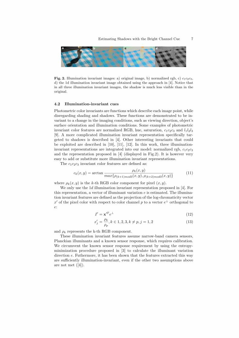
Illumination-invariant image cues are not sufficient in the general case, how-ever, and more complicated reasoning is necessary for more accurate shadowdetection. An example of this can be seen in Fig.2, which shows the illumina-tion invariant features we use for an example image. Edges due to illumination,although dimmer, are still noticeable, while some texture edges are not visible.


Fig. 2. Illumination invariant images: a) original image, b) normalized rgb, c) c1c2c3,d) the 1d illumination invariant image obtained using the approach in [4]. Notice thatin all three illumination invariant images, the shadow is much less visible than in theoriginal.

4.2 Illumination-invariant cues

Photometric color invariants are functions which describe each image point, whiledisregarding shading and shadows. These functions are demonstrated to be in-variant to a change in the imaging conditions, such as viewing direction, object’ssurface orientation and illumination conditions. Some examples of photometricinvariant color features are normalized RGB, hue, saturation, c1c2c3 and l1l2l3[9]. A more complicated illumination invariant representation specifically tar-geted to shadows is described in [4]. Other interesting invariants that couldbe exploited are described in [10], [11], [12]. In this work, three illumination-invariant representations are integrated into our model: normalized rgb, c1c2c3and the representation proposed in [4] (displayed in Fig.2). It is however veryeasy to add or substitute more illumination invariant representations.

The c1c2c3 invariant color features are defined as:

ck(x, y) = arctanρk(x, y)

maxρ(k+1)mod3(x, y), ρ(k+2)mod3(x, y)(11)

where ρk(x, y) is the k-th RGB color component for pixel (x, y).We only use the 1d illumination invariant representation proposed in [4]. For

this representation, a vector of illuminant variation e is estimated. The illumina-tion invariant features are defined as the projection of the log-chromaticity vectorx′ of the pixel color with respect to color channel p to a vector e⊥ orthogonal toe:

I ′ = x′T e⊥ (12)

x′j =ρkρp, k ∈ 1, 2, 3, k 6= p, j = 1, 2 (13)

and ρk represents the k-th RGB component.These illumination invariant features assume narrow-band camera sensors,

Planckian illuminants and a known sensor response, which requires calibration.We circumvent the known sensor response requirement by using the entropy-minimization procedure proposed in [3] to calculate the illuminant variationdirection e. Futhermore, it has been shown that the features extracted this wayare sufficiently illumination-invariant, even if the other two assumptions aboveare not met ([4]).


4.3 The MRF Model

In this section we describe an MRF model that models the relationship of abrightness cue such as the bright channel with the illumination invariant cues,in order to obtain a shadow label for each pixel. Intuitively, through this MRFmodel we seek to obtain labelings that correspond to shadow edges where thereis a transition in the bright channel value, but no significant transition/edgeappears at the same site of an illumination-invariant representation of the image.

The proposed MRF has the topology of a 2D lattice and consists of one nodefor each image pixel i ∈ P. The 4-neighborhood system [13] composes the edgeset E between pixels. The energy of our MRF model has the following form:

E(x) =∑i∈P

φi(xi) +∑

(i,j)∈E

ψi,j(xi, xj), (14)

where φi(xi) is the singleton potential for pixel nodes and ψi,j(xi, xj) is thepairwise potential defined on a pair of neighbor pixels. The singleton potentialhas the following form:

φi(xi) =(xi − Ibright(i)

)2, (15)

where Ibright(i) is the value of the bright channel for pixel i. The pairwise po-tential has the form:

ψi,j(xi, xj) = (xi − xj)2(minkI(k)invar(i)− I

(k)invar(j)

)2, (16)

where I(k)invar(i) is the value of the k-th illumination invariant representation of

the image at pixel i. Note that our MRF model is modular with respect to theillumination invariants used. Other cues can easily be integrated.

The latent variable xi for pixel node i ∈ P represents the quantized shadowintensity at pixel i. We can perform cast shadows detection through a minimiza-tion over the MRF’s energy defined in Eq. 14:

xopt = arg minxE(x) (17)

To minimize the energy of this MRF model we can use existing MRF inferencemethods such as TRW-S [14], the QPBO algorithm [15, 16] with the fusion move[17], etc. The latter was used for the experimental results presented in the nextsection.

5 Experimental Validation

In this section we present qualitative and quantitative results with the brightchannel, and we show further results in an example application in illuminationestimation from shadows.


Fig. 3. Results with images from the dataset by [6]. From left to right: the originalimage; the (unrefined) bright channel; the bright channel refined using confidence es-timation; the bright channel refined using the MRF model; the ground truth. Theseexamples show advantages and weaknesses of the two refinement methods.

5.1 Quantitative Evaluation

We evaluated our approach on the dataset provided by [6], which contains 356images and the corresponding ground truth for the shadow labels. In order toconvert the bright channel values to a 0-1 shadow labeling, we used simple thresh-olding. The pixel classification rates are presented in table 1. Example resultscan be found in Fig.3. Fig.5 shows a case where our algorithm fails, due to verylarge uniformly dark surfaces.

method classification rate (%) false positives (%) false negatives (%)

bright channel 83.52 13.16 3.31

bright channel + confidence 84.61 11.21 4.17

bright channel + MRF 85.88 8.83 5.28

brightness + MRF 52.53 46.31 1.15

Table 1. Pixel classification results for the unrefined bright channel (using a singlepatch size κ = 6 pixels); the bright channel refined using confidence values and 4scales; our MRF model with the bright channel (using a single patch size κ = 6 pixels);and our MRF model with pixel brightness in the LAB color space instead of the brightchannel for the singleton potentials.

5.2 Simple Illumination Estimation

We can use the bright channel image to perform illumination estimation fromshadows. As a proof of concept, we describe a very simple voting method in


Algorithm 1, which is in most cases able to recover an illumination estimategiven simple 3D geometry of the scene.

Algorithm 1 Voting to initialize illumination estimate

Lights Set: L ← ∅Direction Set: D ← all the nodes of a unit geodesic spherePixel Set: P ← all the pixels in the observed imageloop

votes[d] ← 0, ∀d ∈ Dfor all pixel i ∈ P do

for all direction d ∈ D \ L doif Ibright(i) < θS and ∀d′ ∈ L, ci(d′) = 0 then

if ci(d) = 1 then votes[d]← votes[d] + 1else

if ci(d) = 0 then votes[d]← votes[d] + 1d∗ ← arg maxd(votes[d])Pd∗ ← i|ci(d∗) = 1 and ∀d 6= d∗, ci(d) = 0αd∗ ← median

1−Ibright(i)

max−n(p(i))·d∗,0

i∈Pd∗

if αd∗ < εα thenstop the loop

L ← L ∪ (d∗, αd∗)

The idea is that, shadow pixels that are not explained from the discoveredlight sources vote for the occluded light directions. The pixels that are not inshadow vote for the directions that are not occluded. After discovering a newlight source direction, we estimate the associated intensity using the median ofthe bright channel values of pixels in the shadow of this new light source. Theprocess of discovering new lights stops when the current discovered light doesnot have a significant contribution to the shadows in the scene. To ensure evensampling of the illumination environment, we choose the nodes of a geodesicsphere of unit radius as the set of potential light directions [18]. The results ofthe voting algorithm are used to initialize the MRF both in terms of topologyand search space leading to more efficient use of discrete optimization. Whenavailable, the number of light sources can also be set manually.

We present results on illumination estimation on images of cars collectedfrom Flickr (Fig.4). The geometry used in this case was a 3D bounding boxrepresenting the car in each image, and a plane representing the ground. Thecamera parameters were matched by hand so that the 3D model’s projectionwould roughly coincide with the car in the image.

6 Conclusions

In this paper, we presented a simple but effective image cue for the extractionof shadows from a single image, the bright channel cue. We discussed the lim-


Fig. 4. Results with images of cars collected from Flickr. Top row: the original imageand a synthetic sun dial rendered with the estimated illumination; Bottom row: therefined bright channel. The geometry consists of the ground plane and a single boundingbox for the car.

itations of this cue, and presented a way to deal with them, by examining thebright channel values at multiple scales and computing confidence values foreach dark region using a shadow-dependent feature, such as hue. We furtherdescribed an MRF model as an alternative way to refine the bright channel cueby combining it with a number of illumination-invariant representations. In theresults, we computed the classification accuracy for shadow pixels on a publiclyavailable dataset, we showed examples of the resulting shadow estimates, andwe discussed one potential application of the bright channel cue in illuminationestimation from shadows. In this application, the low false-negative rate and therelatively accurate shadow estimate we can get from this simple cue makes itpossible to tackle a hard problem such illumination estimation with rough ge-ometry information in natural images using simple algorithms such as the votingalgorithm we described. In the future, we are interested in incorporating this cuein a more complex shadow detection framework.

Acknowledgments: This work was partially supported by NIH grants 5R01EB7530-2,1R01DA020949-01 and NSF grants CNS-0627645, IIS-0916286, CNS-0721701.

Fig. 5. A failure case: from left to right, the original image, the bright channel, andthe refined bright channel. The uniformly dark road surface is identified as a shadow.


References

1. Salvador, E., Cavallaro, A., Ebrahimi, T.: Cast shadow segmentation using invari-ant color features. Computer Vision and Image Understanding 95 (2004) 238–259

2. Levin, A., Lischinski, D., Weiss, Y.: A closed-form solution to natural image mat-ting. IEEE Transactions on Pattern Analysis and Machine Intelligence 30 (2008)228–242

3. Finlayson, G., Drew, M., Lu, C.: Intrinsic images by entropy minimization. In:European Conference on Computer Vision (ECCV). (2004)

4. Finlayson, G., Hordley, S., Lu, C., Drew, M.: On the removal of shadows fromimages. IEEE Transactions on Pattern Analysis and Machine Intelligence 28 (2006)59–68

5. Shor, Y., Lischinski, D.: The shadow meets the mask: Pyramid-based shadowremoval. Computer Graphics Forum 27 (2008) 577–586

6. Zhu, J., Samuel, K.G.G., Masood, S., Tappen, M.F.: Learning to recognize shadowsin monochromatic natural images. In: IEEE Computer Society Conference onComputer Vision and Pattern Recognition (CVPR 2010). (2010)

7. He, K., Sun, J., Tang, X.: Single image haze removal using dark channel prior. In:IEEE Computer Society Conference on Computer Vision and Pattern Recognition(CVPR). (2009)

8. Gonzalez, R.C., Woods, R.E.: Digital Image Processing (3rd Edition). Prentice-Hall, Inc. (2006)

9. Gevers, T., Smeulders, A.W.M.: Color based object recognition. Pattern Recog-nition 32 (1997) 453–464

10. Geusebroek, J.M., van den Boomgaard, R., Smeulders, A.W.M., Geerts, H.: Colorinvariance. IEEE Transactions on Pattern Analysis and Machine Intelligence 23(2001) 1338–1350

11. van de Weijer, J., Gevers, T., Geusebroek, J.M.: Edge and corner detection byphotometric quasi-invariants. IEEE Transactions on Pattern Analysis and MachineIntelligence 27 (2005)

12. Diplaros, A., Gevers, T., Patras, I.: Combining color and shape information forillumination-viewpoint invariant object recognition. IEEE Trans. on Image Pro-cessing 15 (2006) 1–11

13. Boykov, Y., Funka-lea, G.: Graph cuts and efficient n-d image segmentation. In-ternational Journal of Computer Vision 70 (2006) 109–131

14. Kolmogorov, V.: Convergent tree-reweighted message passing for energy minimiza-tion. IEEE Transactions on Pattern Analysis and Machine Intelligence 28 (2006)1568–1583

15. Hammer, P.L., Hansen, P., Simeone, B.: Roof duality, complementation and per-sistency in quadratic 0-1 optimization. Mathematical Programming 28 (1984)121–155

16. Kolmogorov, V., Rother, C.: Minimizing nonsubmodular functions with graphcuts-a review. IEEE Transactions on Pattern Analysis and Machine Intelligence29 (2007) 1274–1279

17. Lempitsky, V., Rother, C., Roth, S., Blake, A.: Fusion moves for markov randomfield optimization. IEEE Transactions on Pattern Analysis and Machine Intelli-gence 32 (2010) 1392–1405

18. Sato, I., Sato, Y., Ikeuchi, K.: Illumination from shadows. IEEE Transactions onPattern Analysis and Machine Intelligence 25 (2003) 290–300

Documents

Estimating Shadows with the Bright Channel Cue