Estimating relative needs formulae for new forms of …eprints.lse.ac.uk/59073/1/__lse.ac.uk_storage_LIBRARY_Secondary... · The number of people satisfying eligibility tests for

f

University of Kent

University of Kent Cornwallis Building Canterbury Kent CT2 7NF Tel: 01227 823963

[email protected]

London School of Economics

London School of Economics LSE Health & Social Care Houghton Street London WC2A 2AE Tel: 020 7955 6238 [email protected]

Estimating relative needs formulae for new forms of social care support: using an extrapolation method Interim working paper

Julien Forder and Florin Vadean

Personal Social Services Research Unit PSSRU Discussion paper 2877 July 2014

2

Acknowledgement This report is independent research commissioned and funded by the Department of Health Policy Research Programme (Study to Review and Update RNF Allocation Formulae for Adult Social Care, 056/0018). The views expressed in this publication are those of the author(s) and not necessarily those of the Department of Health.

We would like to thank Olena Nizalova, Jose-Luis Fernandez and Jane Dennett for their support with this report. Furthermore, we are very grateful for the comments and suggestions from Sarah Horne, Jonathon White and other colleagues in DH, DCLG and DWP.

We also like to thank the local authorities that took part in the research and provided data, and members of the advisory panel for their invaluable comments.

Contents Acknowledgement ..............................................................................................................................2

Executive Summary.............................................................................................................................4

Introduction........................................................................................................................................4

Key concepts.......................................................................................................................................4

Methods .............................................................................................................................................5

Empirical analysis ................................................................................................................................6

Assessment and DPA estimations........................................................................................................6

Results ................................................................................................................................................7

Discussion ...........................................................................................................................................9

Introduction...................................................................................................................................... 10

Key concepts..................................................................................................................................... 13

Analytical framework ........................................................................................................................ 14

Assessment formula ...................................................................................................................... 16

Deferred payment agreements ..................................................................................................... 16

Empirical analysis .............................................................................................................................. 17

Estimating financial eligibility ........................................................................................................ 17

Estimating need eligibility ............................................................................................................. 18

Assessment and DPA estimations...................................................................................................... 20

Estimation results ............................................................................................................................. 21

Descriptive statistics ..................................................................................................................... 21

Count models................................................................................................................................ 21

Model performance: Prediction correlations ............................................................................. 23

Eligibility models ........................................................................................................................... 24

Relative need formulae ..................................................................................................................... 26

Exemplifications ............................................................................................................................ 28

3

Discussion ......................................................................................................................................... 29

Sensitivity and robustness ............................................................................................................. 30

Policy implications ........................................................................................................................ 32

Annex 1. Analytical framework ......................................................................................................... 33

Predicting need ............................................................................................................................. 33

New forms of support ................................................................................................................... 34

Assessment formula .................................................................................................................. 34

Deferred payment agreement ................................................................................................... 34

Estimating financial eligibility ........................................................................................................ 34

Estimating need eligibility ............................................................................................................. 35

Linear formulae............................................................................................................................. 36

Annex 2. Data sources and manipulation .......................................................................................... 37

Population Estimates at July 2012 ................................................................................................. 37

Benefits Claimants Data ................................................................................................................ 38

Number of Care Home Beds .......................................................................................................... 38

Residential Care Clients aged 65 and over ..................................................................................... 39

Non-residential Care Clients aged 65 and over .............................................................................. 40

Census 2011 data .......................................................................................................................... 42

English Longitudinal Study of Ageing data ..................................................................................... 43

Annex 3. Exemplifications ................................................................................................................. 52

References ........................................................................................................................................ 56

4

Executive Summary

Introduction 1. Local authorities in England have responsibility for securing adult social care for their local

populations. Historically, social care support has included: services such as home care and residential care; personal budgets and direct payments; equipment; and also some professional support like social work. The majority of public social care funding, however, comes from central Government, and is distributed to local authorities in the form of both open-ended grants (the majority) and some ring-fenced grants.

2. Following the Layfield enquiry in 1976 (Cmnd 6453 1976) central Government grants have been allocated to local authorities using a formula to help account for differences in local funding requirements (Bebbington and Davies 1980). The latest incarnation – in operation since 2006/7 – is the relative need formula (RNF) (Darton, Forder et al. 2010).

3. The fundamental principle underpinning the use of allocation formulas is to ensure equal opportunity of access to ‘support’ for equal need. The conventional way to interpret this principle is that each council should have, after their allocation, sufficient net funding so that they can provide an equivalent level of support (services or otherwise) to all people in their local population who would satisfy national standard eligibility conditions (Gravelle, Sutton et al. 2003; Smith 2007).

4. The number of people satisfying eligibility tests for public support for social are, and the amount of that support, will vary between local authorities according to a range of ‘need-related’ and wealth/income factors. These factors can be largely regarded as being ‘exogenous’, beyond the (reasonable) control of the local council, and therefore funding allocations should be adjusted to compensate local authorities accordingly.

5. Following implementation of the Care Act 2014 local authorities will be required to meet the costs of care for people whose cumulative cost of care has exceeded a certain threshold amount – the ‘cap’ limit. In order to determine people’s progression towards the cap, authorities will be required to regularly assess the needs of all people with possible care needs. The Care Act 2014 will also introduce a new deferred payment scheme. This policy allows people to defer paying assessed charges for their care from local authorities until a later date, up to their time of death

6. We consider the new forms of support to be provided by local authorities as arising from the Care Act 2014: the additional responsibility for the assessment of need and the provision of deferred payment agreements (DPAs). The main aim is to develop two relative needs formulae that will determine funding allocations to local authorities for these new responsibilities.

Key concepts 7. The principle of formula allocations is that local authorities are compensated for externally

driven cost variation. In applying this principle we need to determine what factors are considered external, and so beyond the control of the local authority, and which are not. The main drivers of cost for social care are the needs-characteristics of the local population. Needs factors are the core variables in relative needs formulae and can be regarded as external.

8. Some other factors, such as council preferences about setting local eligibility thresholds, are clearly within council control and should not be ‘controlled for’ in the formula. But other factors are between these two cases. At least three merit further discussion in the context of this analysis.

5

a. First, the supply of care services. Most LAs commission services from independent sector providers, and so do not have direct control over that form of supply. Nonetheless, LAs do have powers to directly provide services and are able to manage local markets to some extent. For this reason, supply conditions were not treated as exogenous in developing relative needs formulae.

b. The second factor concerns the demand for services. Differences in demand can lead to variation in the use of services beyond that expected on the basis of (eligible) need alone. In this study we did not include these factors in the formula because they are at least in part affected by LA policies. In particular, LAs operate with need-assessment criteria with regard to publicly-funded care, including for the new responsibilities. Also, more pragmatically, behavioural effects are very hard to anticipate and model. For example, there are no sound data or theoretical models on which to predict demand for assessments or DPA.

c. The third is population sparsity. The main argument is that the costs of providing services could be higher in rural areas than in urban areas. Formula funding directly accounts for differences in unit cost by applying the area cost adjustment. There may also be supply effects, but these are treated as above i.e. excluded from the formula. There could be an argument that rurality implies some direct need effect. Nonetheless, in theory, the other direct need proxies used in the analysis should account for this effect.

9. The general approach was not to include factors in the formulae unless they were clearly considered to be external. The concern otherwise is that by including factors which could be affected by LA policies, the amount of ‘compensatory’ funding an LA receives would become partly under its control.

Methods 10. Relative needs formulae in social care are generally determined by using data about the

support/services that local authorities currently provide. In this case we are concerned with new forms of support and so lack relevant utilisation data. Nonetheless, we can assume that the need-driven uptake of these new forms of support will be directly proportionate to the number of people that would satisfy the need test that underpins current social care support. Neither assessments nor DPAs will be subject to the current financial means-test for social care, although DPAs will be subject to new financial eligibility conditions.

11. We therefore required a measure of the number of people who would satisfy the need test for this analysis. Available datasets provide a range of relevant indicators related to need e.g. rates of attendance allowance uptake, rates of long-standing illness in the population, age, sex and so on. However, for the purposes of funding allocations, particularly into the future, we required a single index of need for each LA that combines the contribution of all these factors. One way of doing this was to statistically model the social care needs test using data on the current use of public social care. Then we could estimate – using regression analysis – how far these indicators ‘explain’ current social care utilisation (service user numbers). A formula for a relative need index can be calculated on this basis.

12. The problem with using social care utilisation data is that current utilisation rates will be determined by the financial means-test, LA preferences/efficiencies and current supply patterns, as well as by the need test. These non-need influences had to be removed or ‘cleaned’.

6

13. Supply factors were cleaned by including a supply variable directly in the regression analysis. The relative effect of supply was then removed by setting this variable to a constant for all LAs. Similarly, LA effects were estimated and removed by using LA dummy variables.

14. The financial means-test is more difficult to clean because it is determined by variables that also explain need: e.g. living alone and income/income benefits. If we set all relevant financial indicator variables to a constant for each LA, we risk under-measuring some important aspects of need differences. We tackled this problem by estimating the effect of relevant financial indicator variables on a simulated version of the current financial eligibility test.

15. Once these non-need influences were removed, the result was an equation predicting differences in relative need between LAs, and this was used to calculate a relative need equation for additional assessments.

16. The simulation approach could also be used to model the new DPA financial eligibility test. In the same way as above, the results could be used in combination with the needs test to determine likely up-take patterns for DPAs in each LA. By estimating the relationship between these expected up-take patterns and relevant exogenous factors, we had a basis for estimating a relative needs formula in the DPA case.

17. One of the important benefits of using data on existing local authority-funded services is that this approach avoids problems of out-of-area placement. We use data on what LAs spend, not on what services are used within the local authorities.

Empirical analysis 18. Two datasets were used. First, we constructed a (small) area dataset comprising data on the

numbers of LA-supported clients and routinely-available need and wealth variables such as rates of benefit uptake and Census variables. These data were collected for each lower super-output area (LSOA) – a standard geographical unit – in a final sample of 53 LAs, giving a total of around 14,000 LSOAs. Data for LA-supported clients were provided directly from LAs at LSOA level.

19. The second dataset was the English Longitudinal Survey of Ageing (ELSA). This dataset has a wide range of data about individuals in the survey, including information about their needs-related characteristics and their wealth and income, including benefit uptake.

20. Five waves of ELSA were combined (with financial variables inflated to be in line with the last wave). The sample of people aged 65 and over (or 65+ in shorthand) was selected. This provided 25,420 observations for people aged 65+. These data were then reweighted so that rates of home ownership, living alone and pension credit uptake were in line with rates in the LSOA data.

21. The small area data were used to model the combined effect of local authority need and financial eligibility. The ELSA data were used to directly simulate (a) the financial means-test for current social care support and (b) the new test for DPA eligibility. The results could be used to remove the effect of the current financial means-test, as outlined above.

Assessment and DPA estimations 22. A relative need formula for assessments was estimated for both people with a residential care

need and with a non-residential care need. The following steps were repeated for each case:

a. We used a regression model to estimate the probability that a person satisfies the current financial means-test (퐸) using ELSA data with wealth and need variables (ones that are also available at small area level).

7

b. We used another regression model to estimate the numbers of people in an LSOA that have LA-supported services – i.e. that satisfy both need and financial means-test (푅 + 퐸) – with need, wealth and supply variables.

c. The predicted values from these two estimations (steps a. and b.) were used to calculate the number of people in an LSOA that would pass the needs test (only) (푅).

i. We removed LA-level effects and supply effects using their national average values from the estimation at step b.

d. A regression model was used to estimate an equation for the number of people in an LSOA that would pass the needs test only (푅) (as determined at step c.) in terms of need, wealth, supply and (population) scaling variables.

i. We calibrated between the two estimations (steps a. and b.) by scaling all the coefficients in this equation using a common factor so that the net effect of home ownership on the numbers of people satisfying the need test was zero.

e. Statistical error for the process in steps b. to d. was estimated (using bootstrapping). f. A linear approximation was calculated for the coefficients from the equation in step d.

This involved calculating the change in the predicted numbers with need for small changes in each need-related and wealth variable from their sample mean values.

23. An additional assessments formula was found by subtracting the LA-supported clients (linear) equation (푅 + 퐸) from the linear equation for numbers of people passing the need test (푅).

24. The DPA formula was produced in a similar way with the predicted value of DPA eligibility (퐷) also applied at step c. to produce a value for the expected count of DPA-eligible people in each LSOA, and in total for the LA.

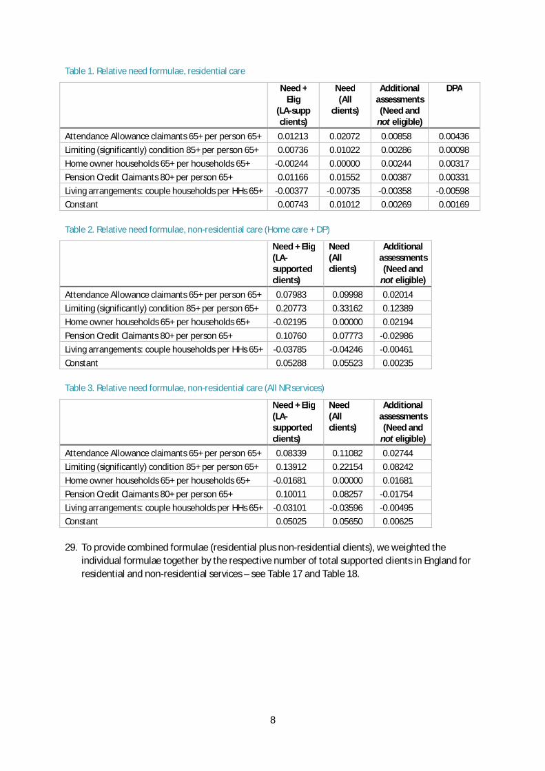
Results 25. The estimations used the following variables:

Need: Supply: Attendance Allowance claimants 65+ per capita 65+ Total care home beds per MSOA per MSOA pop 65+ Limiting (significantly) condition 85+ per capita 65+ Population/scale: Living arrangements: couples per households 65+ Population 65+ (log) Wealth/income: Sparsity: Home owner household 65+ per households 65+ Population density (total pop per hectare) Pension Credit Claimants 80+ per capita 65+

26. Both age and gender variables were initially included but proved not to be significant. Sparsity

was not significant in the residential care estimation but was for non-residential care. Relative need formulae (RNFs) were derived holding supply, scale and sparsity constant.

27. Table 14 give RNFs for residential care. For non-residential care, we used two different specifications: the first with the number of clients using either LA-funded home care or direct payments (Table 15); and the second with the number of clients using any LA-funded non-residential care service (Table 16). The former variable had fewer missing values.

28. The condition whereby a person satisfies the need test but is not financially eligible (Need and not eligible) is calculated by subtracting the first column from the second column. It gives an RNF for additional assessments. The DPA formula only applies in the residential care case.

8

Table 1. Relative need formulae, residential care

Need + Elig

(LA-supp clients)

Need (All

clients)

Additional assessments (Need and

not eligible)

DPA

Attendance Allowance claimants 65+ per person 65+ 0.01213 0.02072 0.00858 0.00436 Limiting (significantly) condition 85+ per person 65+ 0.00736 0.01022 0.00286 0.00098 Home owner households 65+ per households 65+ -0.00244 0.00000 0.00244 0.00317 Pension Credit Claimants 80+ per person 65+ 0.01166 0.01552 0.00387 0.00331 Living arrangements: couple households per HHs 65+ -0.00377 -0.00735 -0.00358 -0.00598 Constant 0.00743 0.01012 0.00269 0.00169 Table 2. Relative need formulae, non-residential care (Home care + DP)

Need + Elig (LA-supported clients)

Need (All clients)


not eligible) Attendance Allowance claimants 65+ per person 65+ 0.07983 0.09998 0.02014 Limiting (significantly) condition 85+ per person 65+ 0.20773 0.33162 0.12389 Home owner households 65+ per households 65+ -0.02195 0.00000 0.02194 Pension Credit Claimants 80+ per person 65+ 0.10760 0.07773 -0.02986 Living arrangements: couple households per HHs 65+ -0.03785 -0.04246 -0.00461 Constant 0.05288 0.05523 0.00235 Table 3. Relative need formulae, non-residential care (All NR services)


Need (All clients)


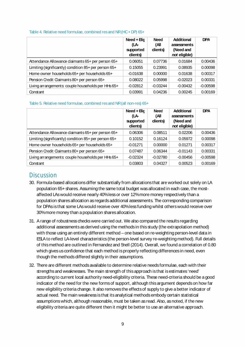
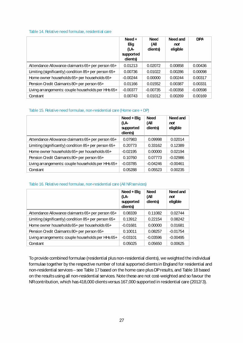
not eligible) Attendance Allowance claimants 65+ per person 65+ 0.08339 0.11082 0.02744 Limiting (significantly) condition 85+ per person 65+ 0.13912 0.22154 0.08242 Home owner households 65+ per households 65+ -0.01681 0.00000 0.01681 Pension Credit Claimants 80+ per person 65+ 0.10011 0.08257 -0.01754 Living arrangements: couple households per HHs 65+ -0.03101 -0.03596 -0.00495 Constant 0.05025 0.05650 0.00625 29. To provide combined formulae (residential plus non-residential clients), we weighted the

individual formulae together by the respective number of total supported clients in England for residential and non-residential services – see Table 17 and Table 18.

9

Table 4. Relative need formulae, combined res and NR (HC + DP) 65+

Need + Elig (LA-

supported clients)

Need (All

clients)


not eligible)

DPA

Attendance Allowance claimants 65+ per person 65+ 0.06051 0.07736 0.01684 0.00436 Limiting (significantly) condition 85+ per person 65+ 0.15055 0.23991 0.08935 0.00098 Home owner households 65+ per households 65+ -0.01638 0.00000 0.01638 0.00317 Pension Credit Claimants 80+ per person 65+ 0.08022 0.05998 -0.02023 0.00331 Living arrangements: couple households per HHs 65+ -0.02812 -0.03244 -0.00432 -0.00598 Constant 0.03991 0.04236 0.00245 0.00169 Table 5. Relative need formulae, combined res and NR (all non-res) 65+

Need + Elig (LA-

supported clients)

Need (All

clients)


not eligible)

DPA

Attendance Allowance claimants 65+ per person 65+ 0.06306 0.08511 0.02206 0.00436 Limiting (significantly) condition 85+ per person 65+ 0.10152 0.16124 0.05972 0.00098 Home owner households 65+ per households 65+ -0.01271 0.00000 0.01271 0.00317 Pension Credit Claimants 80+ per person 65+ 0.07487 0.06344 -0.01143 0.00331 Living arrangements: couple households per HHs 65+ -0.02324 -0.02780 -0.00456 -0.00598 Constant 0.03803 0.04327 0.00523 0.00169

Discussion 30. Formula-based allocations differ substantially from allocations that are worked out solely on LA

population 65+ shares. Assuming the same total budget was allocated in each case, the most-affected LAs would receive nearly 40% less or over 12% more money respectively than a population shares allocation as regards additional assessments. The corresponding comparison for DPAs is that some LAs would receive over 40% less funding whilst others would receive over 30% more money than a population shares allocation.

31. A range of robustness checks were carried out. We also compared the results regarding additional assessments as derived using the methods in this study (the extrapolation method) with those using an entirely different method – one based on re-weighting person-level data in ESLA to reflect LA-level characteristics (the person-level survey re-weighting method). Full details of this method are outlined in Fernandez and Snell (2014). Overall, we found a correlation of 0.80 which gives us confidence that each method is properly reflecting differences in need, even though the methods differed slightly in their assumptions.

32. There are different methods available to determine relative needs formulae, each with their strengths and weaknesses. The main strength of this approach is that is estimates ‘need’ according to current local authority need-eligibility criteria. These need-criteria should be a good indicator of the need for the new forms of support, although this argument depends on how far new eligibility criteria change. It also removes the effects of supply to give a better indicator of actual need. The main weakness is that its analytical methods embody certain statistical assumptions which, although reasonable, must be taken as read. Also, as noted, if the new eligibility criteria are quite different then it might be better to use an alternative approach.

10

Introduction Local authorities in England have responsibility for securing adult social care for their local populations. Historically, social care support has included: services such as home care and residential care; personal budgets and direct payments; equipment; and also some professional support like social work. The majority of public social care funding, however, comes from central Government, and is distributed to local authorities in the form of both open-ended grants (the majority) and some ring-fenced grants.

Following the Layfield enquiry in 1976 (Cmnd 6453 1976) central Government grants have been allocated to local authorities using a formula to help account for differences in local funding requirements (Bebbington and Davies 1980). The latest incarnation – in operation since 2006/7 – is the relative need formula (RNF) (Darton, Forder et al. 2010).

The fundamental principle underpinning the use of allocation formulas is to ensure equal opportunity of access to ‘support’ for equal need. The conventional way to interpret this principle is that each council should have, after their allocation, sufficient net funding so that they can provide an equivalent level of support (services or otherwise) to all people in their local population who would satisfy national standard eligibility conditions (Gravelle, Sutton et al. 2003; Smith 2007).

In other words, the objective of the system of Relative Needs Formulae is to provide a way of assessing the relative need for a particular set of services or support by different local authorities. The formulae need to be based on factors that are measured and updated routinely, which have a demonstrable and quantifiable link with needs and costs, and are outside the influence of local authorities (particularly through past decisions about services). The formulae have to be designed to measure variations in needs between local authorities and costs, other than area costs. They are not concerned with the absolute level of expenditure needed, or with the short-run implications of actual funding arrangements. The current formula contains four components: a need component, a low income adjustment, a sparsity adjustment, and an area cost adjustment.

Two sets of eligibility conditions/tests are relevant for public social care support in general (Wanless, Forder et al. 2006; Forder and Fernández 2009; Fernandez and Forder 2010; Fernandez, Forder et al. 2011). First, the access and support test that determines whether a person should receive support and if so how much, given their condition and circumstances. Second, any financial means test which determines whether a person is eligible for any public support on the basis of relevant non-need criteria, particularly the person’s financial circumstances.

Together these tests determine how much need-related funding is required to meet the national standard. The number of people satisfying these tests and the public cost of their support as dictated by the tests will vary between local authorities according to the size and nature of both ‘need’ and wealth within the local population. These factors can be largely regarded as being ‘exogenous’ beyond the (reasonable) control of the local council, and therefore the funding allocations going to local authorities should be adjusted to reflect differences in these exogenous factors. Relevant factors will include indicators of need, such as rates of disability in the local population. These will largely affect expenditure requirements through the first test. Furthermore, factors will include markers of asset holding and income, which mainly work through the second test – see Box 1. Conventionally, a formula is deployed to account for these exogenous factors and adjust each local authority’s funding allocation accordingly.

This analysis concerns the development of allocation formulae for the new forms of support that councils will need to provide as a result of the Care Act 2014. In particular, it is concerned with those

11

measures that are due to come into effect from April 2015, namely: the additional responsibility on local authorities for the assessment of need, including for people that are currently not eligible for support on the basis of their financial means (i.e. self-payers); and the provision of deferred payment agreements (DPAs).

Following implementation of the Care Act 2014 local authorities will be required to meet the costs of care for people whose cumulative cost of care has exceeded a certain threshold amount – the ‘cap’ limit. In order to determine people’s progression towards the cap, authorities will be required to regularly assess the needs of all people with possible care needs. As a result, LAs can expect to have to undertake significantly more assessments, particularly from people that currently fund their own care. The 2013 DH consultation document suggests that, as a result of the reforms, up to 500,000 more people with eligible care needs could make contact with their local authority in 2016 (Department of Health 2013). This activity will create a new cost burden for councils which will require funding that is allocated by a relative need formula.

The Care Act 2014 will also introduce a new deferred payment scheme. This policy allows people to defer paying assessed charges for their care from local authorities until a later date, up to their time of death. A deferred payment agreement will involve the local authority meeting an agreed proportion of the cost of a care home until the agreed time, with the debt secured against the equity in the person’s housing assets. Since the local authority will have to fund the loan, particularly during the initial period of this policy, additional public funding is likely to be required for LAs to meet this obligation. Again, the relevant funding will be allocated from the centre using a relative needs formula.

The study described in this report was commissioned to examine the needs component for associated RNFs. The main aim of this work is to develop two relative needs formulae that will determine funding allocations to local authorities for these new responsibilities.

Relative needs formulae in social care are generally determined by using data on the support that local authorities currently provide, and establishing (using statistical models) the relationship between exogenous need variables and the amount of that support. In particular, this has involved using data on the current level of publicly-funded social care service utilisation by local populations (Darton, Forder et al. 2010). The methods for determining these relationships allow for the influence of non-exogenous factors when using data on current support.

12

In this case we are concerned with new forms of support, and therefore lack data on actual level of support. Nonetheless, we can assume that the relative need for these new forms of support is directly proportionate to the number of people that would satisfy the need test. This ‘information’ is embodied in current patterns of service utilisation.

The specific aim is to determine the relative proportion of the national cost of assessments and DPAs that each LA will need to fund. Eligibility for both these forms of support will determined by a needs test. Neither will be subject to the current financial means-test for social care, although DPAs will be subject to new financial eligibility conditions.

As regards needs-based eligibility, current datasets provide a range of indicators of need (and different aspects of need) such as rates of AA uptake, rates of LLSI in population, age, sex and so on. These need factors will determine whether a person satisfies the need test. The problem is that the need test embodies a combination of needs-related conditions. We might in principle use just a single need factor e.g. the size of the local older population, but this approach would almost certainly not capture all relevant factors. What we require is a way of combining these indicators into a single index of need for each LA. One way of doing this is to model the current social care needs test. We can see how far these factors explain current social care utilisation (service user numbers) by LAs, using regression analysis. A formula for a relative need index can be estimated on this basis. If we assume that the need for assessments and DPAs is proportionate to this index, then the index can directly serve as a basis for determining funding shares that should go to each LA.

The limitation with using social care provision is that utilisation of support reflects both the current financial means-test and current supply patterns, as well as needs factors.

These influences need to be ‘cleaned’ from the social care utilisation data because they have no basis to inform a relative need formula about assessments and/or DPAs. Leaving these factors in such a formula (e.g. using the current relative needs formula) will bias the results.

Supply factors can be ‘cleaned’ by including a supply variable directly in the regression analysis. The relative effect of supply is then removed by setting this variable to a constant for all LAs.

Box 1 Exogenous factors

Relative needs formulae should therefore include exogenous need factors. They also need to allow for the effects of preferences and supply when establishing the relationship between expenditure requirements and need factors.

The needs factors are likely to include:

Age and sex Marital status Impairment, disability, chronic conditions Environment e.g. housing Informal care Health care provision (endogenous) Affluence Education/socio-economic status Ethnicity

13

The financial means-test is more difficult to clean because it is determined by variables that also explain need i.e. living alone and income/income benefits. If we set all relevant financial indicator variables to a constant for each LA, we risk under-measuring some important aspects of need differences. One way to tackle this problem is to estimate the effect of relevant financial indicator variables on a simulated version of the current financial eligibility test. In theory, the relative contributions of financial indicator variables can then be removed from the estimated need test. One of the steps needed in this process is to calibrate this adjustment. For this purpose we select one of the financial indicator variables that is least likely to also reflect need and then set this value to zero in the need formula. In this analysis we selected home ownership rates as the calibration variable.

The simulation approach can also be used to model the new DPA financial eligibility test. In the same way as above, the results can be used in combination with the needs test to determined likely up-take patterns for DPAs in each LA. By estimating the relationship between these expected up-take patterns and relevant exogenous factors, we have a basis for estimating a relative needs formula in the DPA case.

One of the important benefits of using existing local authority-funded services for estimating relative need is that this avoids problems of out-of-area placement. Many LAs, but particularly those in London, have some residents placed in care homes outside the LA boundaries. These public costs of care for these people generally remains the responsibility of the referring LA. We use data on what LAs spend, not on what services are used within the local authorities, so precluding this issue.

In what follows we outline the analytical framework, discuss data and methods and then provide results. Finally, relative need formulae are presented.

Key concepts The principle of formula allocations is that local authorities are compensated for externally driven cost variation. In applying this principle we need to be able to determine what factors are considered external, and so beyond the control of the local authority, and which are not. The needs-related characteristics of the local population can generally be regarded as external. These characteristics would include indicators of population disability, health, age and age and gender mix, income and wealth characteristics and so on. Needs factors are the core variables in relative needs formulae and would be expected to account for most of the difference in care utilisation patterns between councils.

Some other factors, such as council preferences about setting local eligibility thresholds, are clearly within council control and should not be ‘controlled for’ in the formula. But other factors are between these two cases. At least three merit further discussion in the context of this analysis.

The first is the supply of care services. Most LAs commission services from independent sector providers, and so do not have direct control over that form of supply. Nonetheless, LAs do have powers to directly provide services and are able to manage local markets to some extent. For this reason, we did not treat supply conditions as exogenous in developing relative needs formulae. Relevant factors were included in the underlying analysis to account for supply effects, and so identify need, but these were factors were set to their national average and treated as a constant in the RNFs.

The second consideration relates to factors that drive demand or individual preferences for services, where differences in demand can lead to variation in use of service beyond that expected on the basis of (eligible) need alone. In other words, whilst a certain number of people in an area might be

14

eligible for support, the actual number of people taking up support could differ. Local characteristics such as information, wealth etc. can explain differences in demand. Again in this paper we did not include these factors in the formula because they are at least in part affected by LA policies. In particular, LAs operate with need-assessment criteria with regard to publicly-funded care, including the new responsibilities. As a consequence, for example, any people/families with preferences such that they enter residential care earlier than indicated by LA assessment criteria (by self-funding), would not be eligible for DPAs.

Preferences for care might lead to under-utilisation of care relative to eligible levels in some cases. But again, LAs should be able to influence these factors. Moreover, it would not seem appropriate to have a formula that rewards under-utilisation of care relative to eligible levels. Also, more pragmatically, behavioural effects are very hard to anticipate and model. For example, there are no sound data or theoretical models on which to predict demand for assessments or DPA, as opposed to the numbers who might meet eligibility criteria for these forms of support.

A third factor relates to rurality or population sparsity. The main argument is that the costs of providing could be higher in rural areas than in urban areas. Formula funding directly accounts for differences in wage-driven unit cost by applying the area cost adjustment on top of the relative needs formula. However, differences in the costs of delivering services can also affect the amount of supply, not just the unit cost. For example, in areas with low labour costs and/or low transport costs, the supply of non-residential care would be higher than in high-cost areas, other things equal. As outlined above, we need to isolate supply from need differences and therefore should include supply indicators. For residential care, we did have a direct measure in the form of the total number of available places in care homes in the area. We did not have a similar variable for non-residential care. Rather, we included population density (population per hectare). In treating this variable as a supply indicator it was used in the underlying analysis, but was not incorporated into the relative needs formulae. There could be an argument that rurality implies some direct need effect. Nonetheless, in theory, the other direct need proxies used in the analysis should account for this effect.

The general approach was not to include factors in the formulae unless they were clearly considered to be external. The concern otherwise is that by including factors that could be affected by LA policies, the amount of ‘compensatory’ funding an LA receives would become partly under its control. As such, formula approaches have tended to take the most parsimonious route and only include factors if they are unambiguously exogenous. But ultimately this is a design philosophy.

Analytical framework The two tests that determine access to LA-supported social care for each person are: the needs test and the (financial) eligibility test. For shorthand, we can abbreviate the former as 푅 and the latter as 퐸. Our aim was to determine the nature of the LA needs test 푅, and in particular to estimate the probability that a person satisfies this test. Again as a shorthand, we can denote this probability as 푝(푅). With a suitable measure of this probability, we could use a statistical model to determine how it is affected by relevant exogenous factors that are available in routine data sets. In other words, this would give an equation for need comprising variables as given in Box 1, as we require.

We did not, however, have a direct measure of this probability. The number of people that are LA-supported is directly available data and this number will depend on this probability, but it also depends on the probability that those people also meet the means-test (퐸). Also, we could not simulate the needs test even if we had a suitable dataset, because the needs test guidance

15

(Department of Health 2010; Department of Health 2013) is insufficiently precise and subject to local interpretation (Fernandez and Snell 2012). We could, however, estimate this probability indirectly.

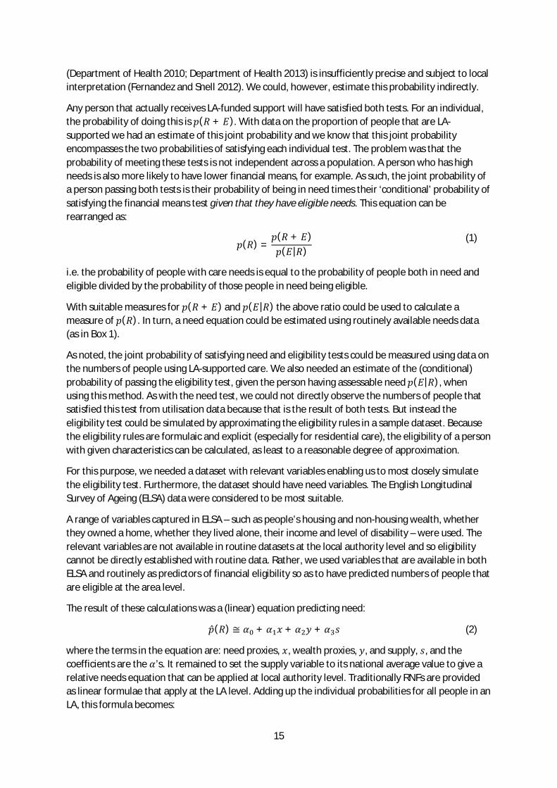
Any person that actually receives LA-funded support will have satisfied both tests. For an individual, the probability of doing this is 푝(푅 + 퐸). With data on the proportion of people that are LA-supported we had an estimate of this joint probability and we know that this joint probability encompasses the two probabilities of satisfying each individual test. The problem was that the probability of meeting these tests is not independent across a population. A person who has high needs is also more likely to have lower financial means, for example. As such, the joint probability of a person passing both tests is their probability of being in need times their ‘conditional’ probability of satisfying the financial means test given that they have eligible needs. This equation can be rearranged as:

푝(푅) =

푝(푅 + 퐸)푝(퐸|푅)

(1)

i.e. the probability of people with care needs is equal to the probability of people both in need and eligible divided by the probability of those people in need being eligible.

With suitable measures for 푝(푅 + 퐸) and 푝(퐸|푅) the above ratio could be used to calculate a measure of 푝(푅). In turn, a need equation could be estimated using routinely available needs data (as in Box 1).

As noted, the joint probability of satisfying need and eligibility tests could be measured using data on the numbers of people using LA-supported care. We also needed an estimate of the (conditional) probability of passing the eligibility test, given the person having assessable need 푝(퐸|푅), when using this method. As with the need test, we could not directly observe the numbers of people that satisfied this test from utilisation data because that is the result of both tests. But instead the eligibility test could be simulated by approximating the eligibility rules in a sample dataset. Because the eligibility rules are formulaic and explicit (especially for residential care), the eligibility of a person with given characteristics can be calculated, as least to a reasonable degree of approximation.

For this purpose, we needed a dataset with relevant variables enabling us to most closely simulate the eligibility test. Furthermore, the dataset should have need variables. The English Longitudinal Survey of Ageing (ELSA) data were considered to be most suitable.

A range of variables captured in ELSA – such as people’s housing and non-housing wealth, whether they owned a home, whether they lived alone, their income and level of disability – were used. The relevant variables are not available in routine datasets at the local authority level and so eligibility cannot be directly established with routine data. Rather, we used variables that are available in both ELSA and routinely as predictors of financial eligibility so as to have predicted numbers of people that are eligible at the area level.

The result of these calculations was a (linear) equation predicting need:

푝̂(푅) ≅ 훼 + 훼 푥 + 훼 푦 + 훼 푠 (2)

where the terms in the equation are: need proxies, 푥, wealth proxies, 푦, and supply, 푠, and the coefficients are the 훼’s. It remained to set the supply variable to its national average value to give a relative needs equation that can be applied at local authority level. Traditionally RNFs are provided as linear formulae that apply at the LA level. Adding up the individual probabilities for all people in an LA, this formula becomes:

16

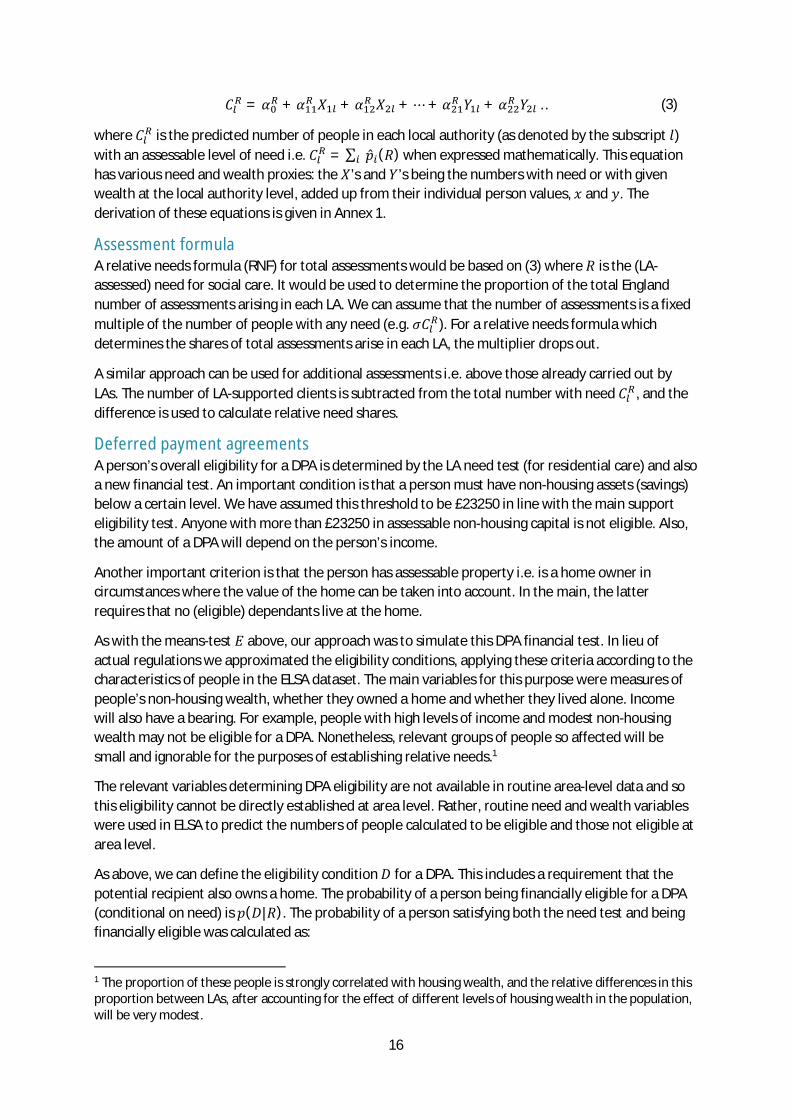
퐶 = 훼 + 훼 푋 + 훼 푋 + ⋯+ 훼 푌 + 훼 푌 … (3)

where 퐶 is the predicted number of people in each local authority (as denoted by the subscript 푙) with an assessable level of need i.e. 퐶 = ∑ 푝̂ (푅) when expressed mathematically. This equation has various need and wealth proxies: the 푋’s and 푌’s being the numbers with need or with given wealth at the local authority level, added up from their individual person values, 푥 and 푦. The derivation of these equations is given in Annex 1.

Assessment formula A relative needs formula (RNF) for total assessments would be based on (3) where 푅 is the (LA-assessed) need for social care. It would be used to determine the proportion of the total England number of assessments arising in each LA. We can assume that the number of assessments is a fixed multiple of the number of people with any need (e.g. 휎퐶 ). For a relative needs formula which determines the shares of total assessments arise in each LA, the multiplier drops out.

A similar approach can be used for additional assessments i.e. above those already carried out by LAs. The number of LA-supported clients is subtracted from the total number with need 퐶 , and the difference is used to calculate relative need shares.

Deferred payment agreements A person’s overall eligibility for a DPA is determined by the LA need test (for residential care) and also a new financial test. An important condition is that a person must have non-housing assets (savings) below a certain level. We have assumed this threshold to be £23250 in line with the main support eligibility test. Anyone with more than £23250 in assessable non-housing capital is not eligible. Also, the amount of a DPA will depend on the person’s income.

Another important criterion is that the person has assessable property i.e. is a home owner in circumstances where the value of the home can be taken into account. In the main, the latter requires that no (eligible) dependants live at the home.

As with the means-test 퐸 above, our approach was to simulate this DPA financial test. In lieu of actual regulations we approximated the eligibility conditions, applying these criteria according to the characteristics of people in the ELSA dataset. The main variables for this purpose were measures of people’s non-housing wealth, whether they owned a home and whether they lived alone. Income will also have a bearing. For example, people with high levels of income and modest non-housing wealth may not be eligible for a DPA. Nonetheless, relevant groups of people so affected will be small and ignorable for the purposes of establishing relative needs.1

The relevant variables determining DPA eligibility are not available in routine area-level data and so this eligibility cannot be directly established at area level. Rather, routine need and wealth variables were used in ELSA to predict the numbers of people calculated to be eligible and those not eligible at area level.

As above, we can define the eligibility condition 퐷 for a DPA. This includes a requirement that the potential recipient also owns a home. The probability of a person being financially eligible for a DPA (conditional on need) is 푝(퐷|푅). The probability of a person satisfying both the need test and being financially eligible was calculated as:

1 The proportion of these people is strongly correlated with housing wealth, and the relative differences in this proportion between LAs, after accounting for the effect of different levels of housing wealth in the population, will be very modest.

17

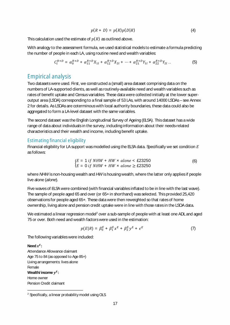
푝(푅 + 퐷) = 푝(푅)푝(퐷|푅) (4)

This calculation used the estimate of 푝(푅) as outlined above.

With analogy to the assessment formula, we used statistical models to estimate a formula predicting the number of people in each LA, using routine need and wealth variables:

퐶 = 훼 + 훼 푋 + 훼 푋 + ⋯+ 훼 푌 + 훼 푌 … (5)

Empirical analysis Two datasets were used. First, we constructed a (small) area dataset comprising data on the numbers of LA-supported clients, as well as routinely-available need and wealth variables such as rates of benefit uptake and Census variables. These data were collected initially at the lower super-output area (LSOA) corresponding to a final sample of 53 LAs, with around 14000 LSOAs – see Annex 2 for details. As LSOAs are coterminous with local authority boundaries, these data could also be aggregated to form a LA-level dataset with the same variables.

The second dataset was the English Longitudinal Survey of Ageing (ELSA). This dataset has a wide range of data about individuals in the survey, including information about their needs-related characteristics and their wealth and income, including benefit uptake.

Estimating financial eligibility Financial eligibility for LA support was modelled using the ELSA data. Specifically we set condition 퐸 as follows:

퐸 = 1 푖푓 푁퐻푊 +퐻푊 × 푎푙표푛푒 < £23250퐸 = 0 푖푓 푁퐻푊 +퐻푊 × 푎푙표푛푒 ≥ £23250 (6)

where NHW is non-housing wealth and HW is housing wealth, where the latter only applies if people live alone (alone).

Five waves of ELSA were combined (with financial variables inflated to be in line with the last wave). The sample of people aged 65 and over (or 65+ in shorthand) was selected. This provided 25,420 observations for people aged 65+. These data were then reweighted so that rates of home ownership, living alone and pension credit uptake were in line with those rates in the LSOA data.

We estimated a linear regression model2 over a sub-sample of people with at least one ADL and aged 75 or over. Both need and wealth factors were used in the estimation:

푝(퐸|푅) = 훽 + 훽 푥 + 훽 푦 + 휖 (7)

The following variables were included:

Need 풙푬: Attendance Allowance claimant Age 75 to 84 (as opposed to Age 85+) Living arrangements: lives alone Female Wealth/income 풚푬: Home owner Pension Credit claimant

2 Specifically, a linear probability model using OLS.

18

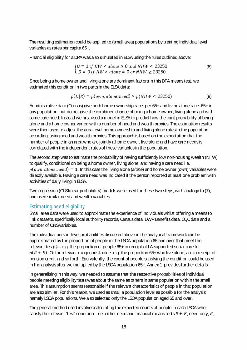
The resulting estimation could be applied to (small area) populations by treating individual level variables as rates per capita 65+.

Financial eligibility for a DPA was also simulated in ELSA using the rules outlined above:

퐷 = 1 푖푓 퐻푊 × 푎푙표푛푒 ≥ 0 푎푛푑 푁퐻푊 < 23250퐷 = 0 푖푓 퐻푊 × 푎푙표푛푒 = 0 표푟 푁퐻푊 ≥ 23250 (8)

Since being a home owner and living alone are dominant factors in this DPA means test, we estimated this condition in two parts in the ELSA data:

푝(퐷|푅) = 푝(표푤푛,푎푙표푛푒,푛푒푒푑) × 푝(푁퐻푊 < 23250) (9)

Administrative data (Census) give both home ownership rates per 65+ and living alone rates 65+ in any population, but do not give the combined chance of being a home owner, living alone and with some care need. Instead we first used a model in ELSA to predict how the joint probability of being alone and a home owner varied with a number of need and wealth proxies. The estimation results were then used to adjust the area-level home ownership and living alone rates in the population according, using need and wealth proxies. This approach is based on the expectation that the number of people in an area who are jointly a home owner, live alone and have care needs is correlated with the independent rates of these variables in the population.

The second step was to estimate the probability of having sufficiently low non-housing wealth (NHW) to qualify, conditional on being a home owner, living alone, and having a care need i.e. 푝(표푤푛, 푎푙표푛푒,푛푒푒푑) = 1. In this case the living alone (alone) and home owner (own) variables were directly available. Having a care need was indicated if the person reported at least one problem with activities of daily living in ELSA.

Two regression (OLS linear probability) models were used for these two steps, with analogy to (7), and used similar need and wealth variables.

Estimating need eligibility Small area data were used to approximate the experience of individuals whilst offering a means to link datasets, specifically local authority records, Census data, DWP Benefits data, CQC data and a number of ONS variables.

The individual person-level probabilities discussed above in the analytical framework can be approximated by the proportion of people in the LSOA population 65 and over that meet the relevant test(s) – e.g. the proportion of people 65+ in receipt of LA-supported social care for 푝(푅 + 퐸). Or for relevant exogenous factors e.g. the proportion 65+ who live alone, are in receipt of pension credit and so forth. Equivalently, the count of people satisfying the condition could be used in the analysis after we multiplied by the LSOA population 65+. Annex 1 provides further details.

In generalising in this way, we needed to assume that the respective probabilities of individual people meeting eligibility tests was about the same as others in same population within the small area. This assumption seems reasonable if the relevant characteristics of people in that population are also similar. For this reason, we used as small a population level as possible for the analysis: namely LSOA populations. We also selected only the LSOA population aged 65 and over.

The general method used involves calculating the expected counts of people in each LSOA who satisfy the relevant ‘test’ condition – i.e. either need and financial means tests 푅 + 퐸, need-only, 푅,

19

and need plus DPA eligibility, 푅 + 퐷 – and then using a regression model to determine the relationship between these counts and LSOA population rates of relevant (routinely-available) need, wealth and supply factors.

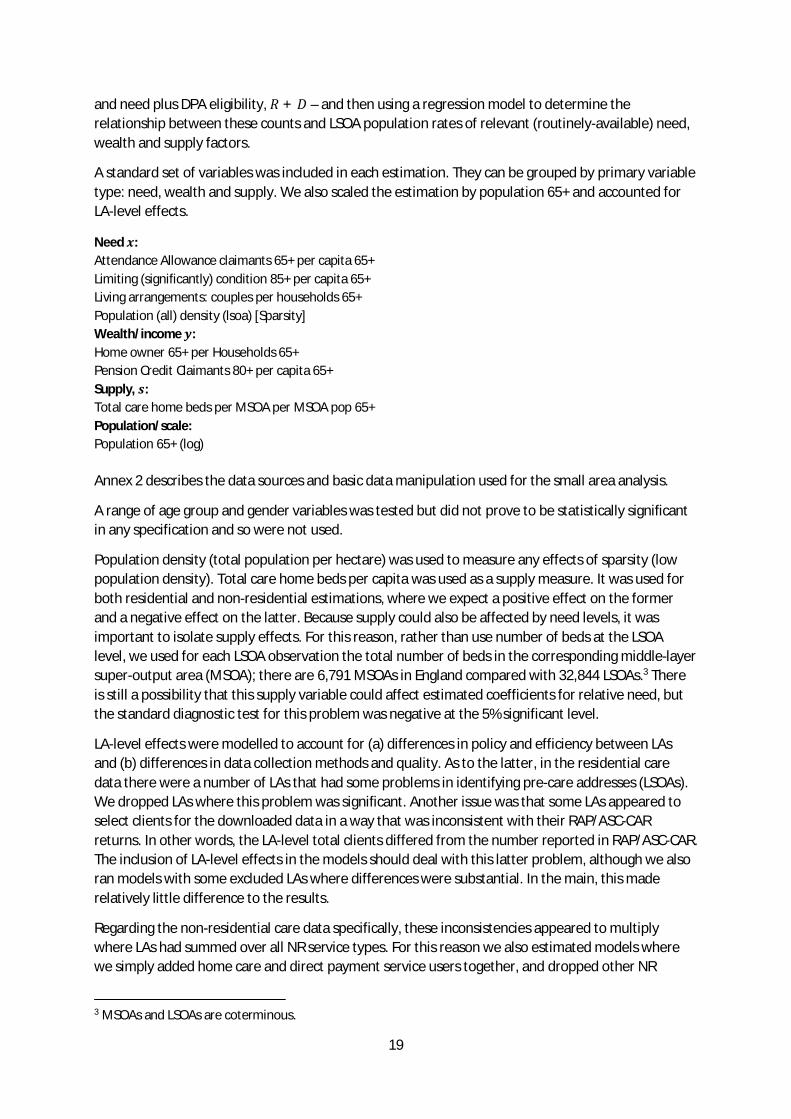
A standard set of variables was included in each estimation. They can be grouped by primary variable type: need, wealth and supply. We also scaled the estimation by population 65+ and accounted for LA-level effects.

Need 풙: Attendance Allowance claimants 65+ per capita 65+ Limiting (significantly) condition 85+ per capita 65+ Living arrangements: couples per households 65+ Population (all) density (lsoa) [Sparsity] Wealth/income 풚: Home owner 65+ per Households 65+ Pension Credit Claimants 80+ per capita 65+ Supply, 풔: Total care home beds per MSOA per MSOA pop 65+ Population/scale: Population 65+ (log) Annex 2 describes the data sources and basic data manipulation used for the small area analysis.

A range of age group and gender variables was tested but did not prove to be statistically significant in any specification and so were not used.

Population density (total population per hectare) was used to measure any effects of sparsity (low population density). Total care home beds per capita was used as a supply measure. It was used for both residential and non-residential estimations, where we expect a positive effect on the former and a negative effect on the latter. Because supply could also be affected by need levels, it was important to isolate supply effects. For this reason, rather than use number of beds at the LSOA level, we used for each LSOA observation the total number of beds in the corresponding middle-layer super-output area (MSOA); there are 6,791 MSOAs in England compared with 32,844 LSOAs.3 There is still a possibility that this supply variable could affect estimated coefficients for relative need, but the standard diagnostic test for this problem was negative at the 5% significant level.

LA-level effects were modelled to account for (a) differences in policy and efficiency between LAs and (b) differences in data collection methods and quality. As to the latter, in the residential care data there were a number of LAs that had some problems in identifying pre-care addresses (LSOAs). We dropped LAs where this problem was significant. Another issue was that some LAs appeared to select clients for the downloaded data in a way that was inconsistent with their RAP/ASC-CAR returns. In other words, the LA-level total clients differed from the number reported in RAP/ASC-CAR. The inclusion of LA-level effects in the models should deal with this latter problem, although we also ran models with some excluded LAs where differences were substantial. In the main, this made relatively little difference to the results.

Regarding the non-residential care data specifically, these inconsistencies appeared to multiply where LAs had summed over all NR service types. For this reason we also estimated models where we simply added home care and direct payment service users together, and dropped other NR

3 MSOAs and LSOAs are coterminous.

20

service use. As shown in the results below, there was relatively little difference in terms of the formulas produced.

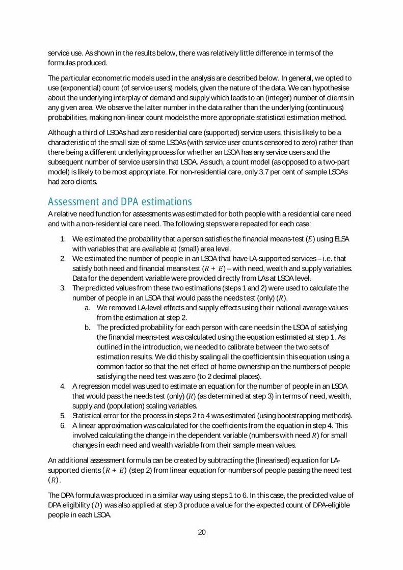
The particular econometric models used in the analysis are described below. In general, we opted to use (exponential) count (of service users) models, given the nature of the data. We can hypothesise about the underlying interplay of demand and supply which leads to an (integer) number of clients in any given area. We observe the latter number in the data rather than the underlying (continuous) probabilities, making non-linear count models the more appropriate statistical estimation method.

Although a third of LSOAs had zero residential care (supported) service users, this is likely to be a characteristic of the small size of some LSOAs (with service user counts censored to zero) rather than there being a different underlying process for whether an LSOA has any service users and the subsequent number of service users in that LSOA. As such, a count model (as opposed to a two-part model) is likely to be most appropriate. For non-residential care, only 3.7 per cent of sample LSOAs had zero clients.

Assessment and DPA estimations A relative need function for assessments was estimated for both people with a residential care need and with a non-residential care need. The following steps were repeated for each case:

1. We estimated the probability that a person satisfies the financial means-test (퐸) using ELSA with variables that are available at (small) area level.

2. We estimated the number of people in an LSOA that have LA-supported services – i.e. that satisfy both need and financial means-test (푅 + 퐸) – with need, wealth and supply variables. Data for the dependent variable were provided directly from LAs at LSOA level.

3. The predicted values from these two estimations (steps 1 and 2) were used to calculate the number of people in an LSOA that would pass the needs test (only) (푅).

a. We removed LA-level effects and supply effects using their national average values from the estimation at step 2.

b. The predicted probability for each person with care needs in the LSOA of satisfying the financial means-test was calculated using the equation estimated at step 1. As outlined in the introduction, we needed to calibrate between the two sets of estimation results. We did this by scaling all the coefficients in this equation using a common factor so that the net effect of home ownership on the numbers of people satisfying the need test was zero (to 2 decimal places).

4. A regression model was used to estimate an equation for the number of people in an LSOA that would pass the needs test (only) (푅) (as determined at step 3) in terms of need, wealth, supply and (population) scaling variables.

5. Statistical error for the process in steps 2 to 4 was estimated (using bootstrapping methods). 6. A linear approximation was calculated for the coefficients from the equation in step 4. This

involved calculating the change in the dependent variable (numbers with need 푅) for small changes in each need and wealth variable from their sample mean values.

An additional assessment formula can be created by subtracting the (linearised) equation for LA-supported clients (푅 + 퐸) (step 2) from linear equation for numbers of people passing the need test (푅).

The DPA formula was produced in a similar way using steps 1 to 6. In this case, the predicted value of DPA eligibility (퐷) was also applied at step 3 produce a value for the expected count of DPA-eligible people in each LSOA.

21

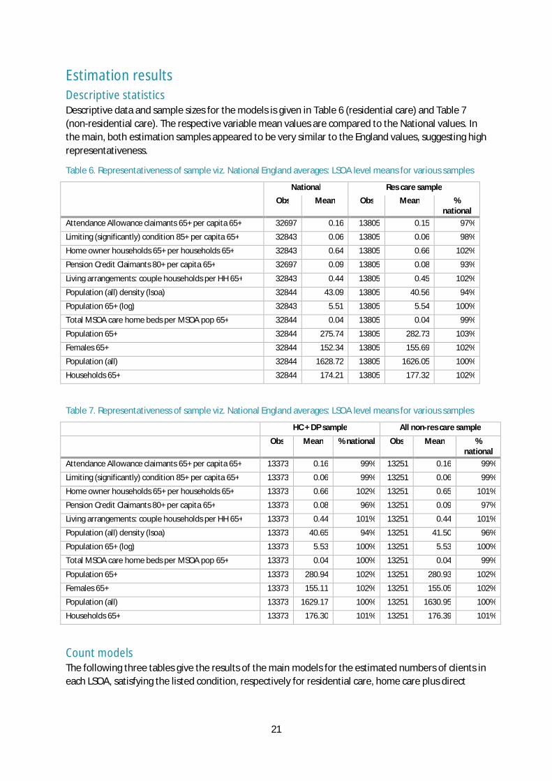
Estimation results Descriptive statistics Descriptive data and sample sizes for the models is given in Table 6 (residential care) and Table 7 (non-residential care). The respective variable mean values are compared to the National values. In the main, both estimation samples appeared to be very similar to the England values, suggesting high representativeness.

Table 6. Representativeness of sample viz. National England averages: LSOA level means for various samples

National Res care sample Obs Mean Obs Mean %

national Attendance Allowance claimants 65+ per capita 65+ 32697 0.16 13805 0.15 97%

Limiting (significantly) condition 85+ per capita 65+ 32843 0.06 13805 0.06 98%

Home owner households 65+ per households 65+ 32843 0.64 13805 0.66 102%

Pension Credit Claimants 80+ per capita 65+ 32697 0.09 13805 0.08 93%

Living arrangements: couple households per HH 65+ 32843 0.44 13805 0.45 102%

Population (all) density (lsoa) 32844 43.09 13805 40.56 94%

Population 65+ (log) 32843 5.51 13805 5.54 100%

Total MSOA care home beds per MSOA pop 65+ 32844 0.04 13805 0.04 99%

Population 65+ 32844 275.74 13805 282.73 103%

Females 65+ 32844 152.34 13805 155.69 102%

Population (all) 32844 1628.72 13805 1626.05 100%

Households 65+ 32844 174.21 13805 177.32 102%

Table 7. Representativeness of sample viz. National England averages: LSOA level means for various samples

HC + DP sample All non-res care sample

Obs Mean % national Obs Mean % national

Attendance Allowance claimants 65+ per capita 65+ 13373 0.16 99% 13251 0.16 99%

Limiting (significantly) condition 85+ per capita 65+ 13373 0.06 99% 13251 0.06 99%

Home owner households 65+ per households 65+ 13373 0.66 102% 13251 0.65 101%

Pension Credit Claimants 80+ per capita 65+ 13373 0.08 96% 13251 0.09 97%

Living arrangements: couple households per HH 65+ 13373 0.44 101% 13251 0.44 101%

Population (all) density (lsoa) 13373 40.65 94% 13251 41.50 96%

Population 65+ (log) 13373 5.53 100% 13251 5.53 100%

Total MSOA care home beds per MSOA pop 65+ 13373 0.04 100% 13251 0.04 99%

Population 65+ 13373 280.94 102% 13251 280.93 102%

Females 65+ 13373 155.11 102% 13251 155.05 102%

Population (all) 13373 1629.17 100% 13251 1630.95 100%

Households 65+ 13373 176.30 101% 13251 176.39 101%

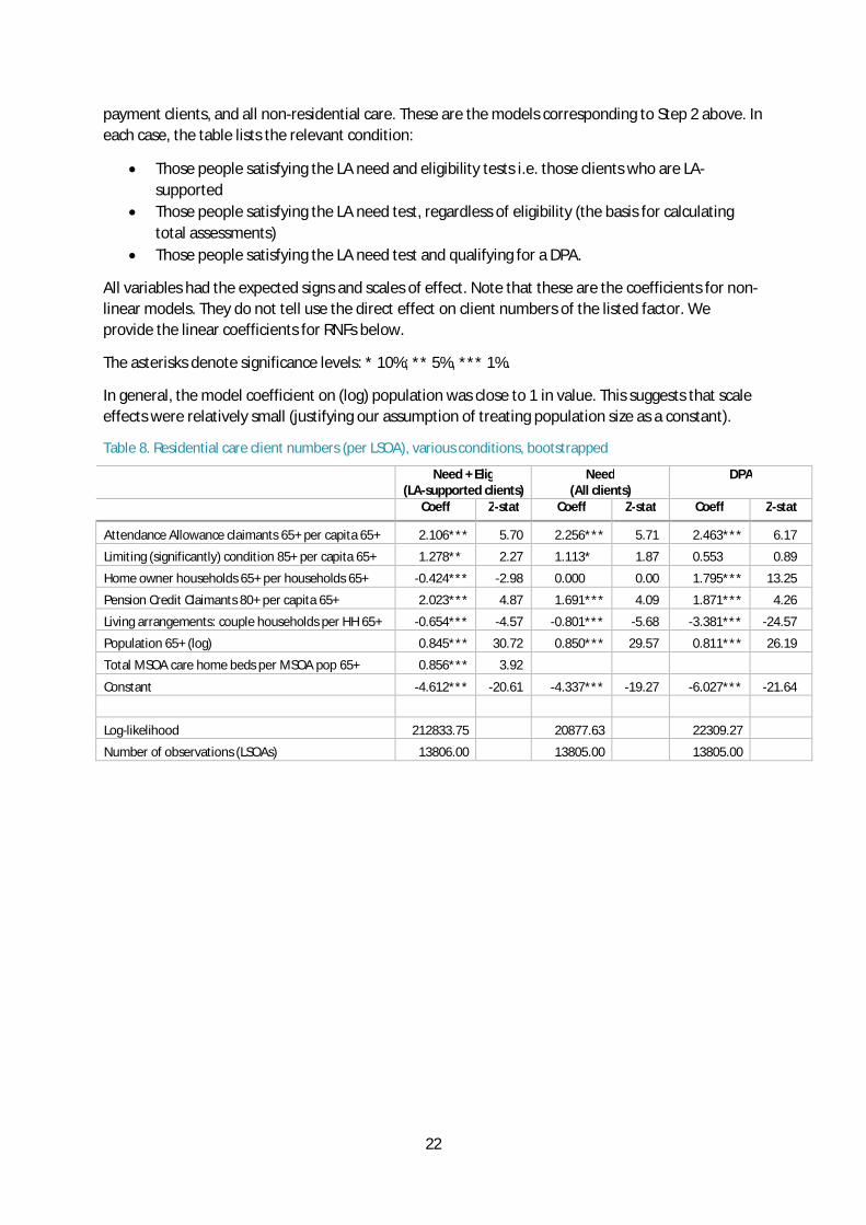
Count models The following three tables give the results of the main models for the estimated numbers of clients in each LSOA, satisfying the listed condition, respectively for residential care, home care plus direct

22

payment clients, and all non-residential care. These are the models corresponding to Step 2 above. In each case, the table lists the relevant condition:

Those people satisfying the LA need and eligibility tests i.e. those clients who are LA-supported

Those people satisfying the LA need test, regardless of eligibility (the basis for calculating total assessments)

Those people satisfying the LA need test and qualifying for a DPA.

All variables had the expected signs and scales of effect. Note that these are the coefficients for non-linear models. They do not tell use the direct effect on client numbers of the listed factor. We provide the linear coefficients for RNFs below.

The asterisks denote significance levels: * 10%; ** 5%, *** 1%.

In general, the model coefficient on (log) population was close to 1 in value. This suggests that scale effects were relatively small (justifying our assumption of treating population size as a constant).

Table 8. Residential care client numbers (per LSOA), various conditions, bootstrapped


Need (All clients)

DPA

Coeff Z-stat Coeff Z-stat Coeff Z-stat

Attendance Allowance claimants 65+ per capita 65+ 2.106*** 5.70 2.256*** 5.71 2.463*** 6.17

Limiting (significantly) condition 85+ per capita 65+ 1.278** 2.27 1.113* 1.87 0.553 0.89

Home owner households 65+ per households 65+ -0.424*** -2.98 0.000 0.00 1.795*** 13.25

Pension Credit Claimants 80+ per capita 65+ 2.023*** 4.87 1.691*** 4.09 1.871*** 4.26

Living arrangements: couple households per HH 65+ -0.654*** -4.57 -0.801*** -5.68 -3.381*** -24.57

Population 65+ (log) 0.845*** 30.72 0.850*** 29.57 0.811*** 26.19

Total MSOA care home beds per MSOA pop 65+ 0.856*** 3.92 Constant -4.612*** -20.61 -4.337*** -19.27 -6.027*** -21.64

Log-likelihood 212833.75

20877.63

22309.27 Number of observations (LSOAs) 13806.00

13805.00

13805.00

23

Table 9. Non-residential care, home care + direct payments: service user numbers, various conditions, bootstrapped


Need (All clients)

Coeff Z-stat Coeff Z-stat

Attendance Allowance claimants 65+ per capita 65+ 1.610*** 9.04 1.392*** 8.31

Limiting (significantly) condition 85+ per capita 65+ 4.189*** 11.74 4.618*** 12.77

Home owner households 65+ per households 65+ -0.443*** -6.85 0.000 0.00

Pension Credit Claimants 80+ per capita 65+ 2.170*** 7.61 1.082*** 3.64

Living arrangements: couple households per households 65+ -0.763*** -6.17 -0.591*** -4.75

Population (all) density (lsoa) 0.001*** 5.87 0.001*** 6.47

Population 65+ (log) 0.933*** 29.23 0.931*** 26.70

Total MSOA care home beds per MSOA pop 65+ -1.243*** -7.52 Constant -3.337*** -20.57 -3.276*** -17.47


-9115.24 Number of observations (LSOAs) 13374

13373

Table 10. Non-residential care, all services: service user numbers, various conditions, bootstrapped


Need (All clients)

Coeff Z-stat Coeff Z-stat

Attendance Allowance claimants 65+ per capita 65+ 1.761*** 11.05 1.629*** 10.07

Limiting (significantly) condition 85+ per capita 65+ 2.939*** 12.71 3.257*** 14.93

Home owner households 65+ per households 65+ -0.355*** -9.55 0.000 0.00

Pension Credit Claimants 80+ per capita 65+ 2.114*** 12.36 1.214*** 6.04

Living arrangements: couple households per households 65+ -0.655*** -8.01 -0.529*** -6.16

Population (all) density (lsoa) 0.001*** 7.22 0.001*** 5.86

Population 65+ (log) 0.889*** 34.29 0.890*** 29.61

Total MSOA care home beds per MSOA pop 65+ -0.803*** -6.16 Constant -2.434*** -14.55 -2.320*** -10.03


-14015.02 Number of observations (LSOAs) 13252

13251

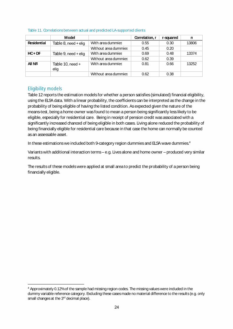
Model performance: Prediction correlations The regression models used in the above estimations are non-linear to account for the nature of the data and do not produce the ‘r-squared’ goodness-of-fit statistics of standard (OLS) estimation. Nonetheless, we can assess the correlation between the data on LA-supported clients and the number of such clients predicted by the statistical model. Table 11 has these results. In general, the two non-residential care models were more closely able to predict the actual number of LA-supported clients.

24

Table 11. Correlations between actual and predicted LA-supported clients

Model Correlation, r r-squared n Residential Table 8, need + elig With area dummies 0.55 0.30 13806

Without area dummies 0.45 0.20 HC + DP Table 9, need + elig With area dummies 0.69 0.48 13374

Without area dummies 0.62 0.39 All NR Table 10, need +

elig With area dummies 0.81 0.66 13252

Without area dummies 0.62 0.38

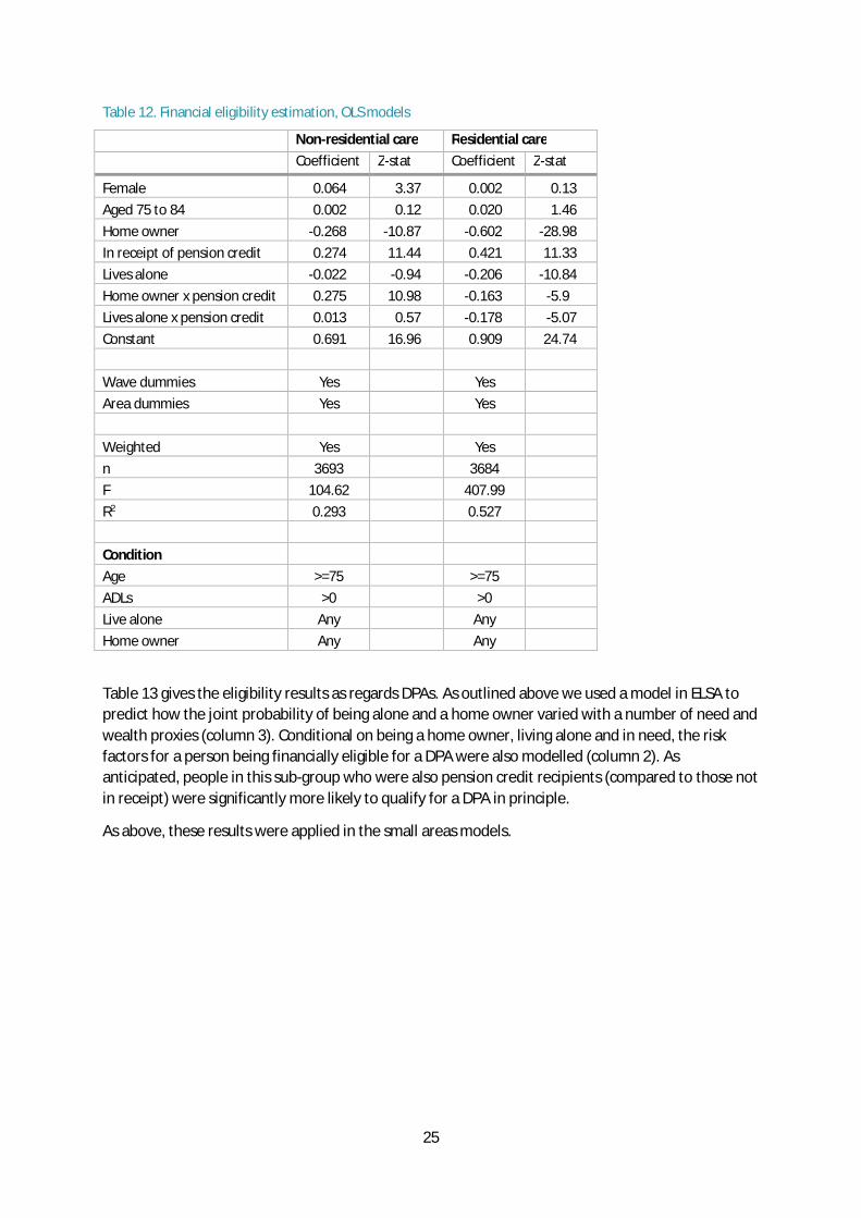
Eligibility models Table 12 reports the estimation models for whether a person satisfies (simulated) financial eligibility, using the ELSA data. With a linear probability, the coefficients can be interpreted as the change in the probability of being eligible of having the listed condition. As expected given the nature of the means-test, being a home owner was found to mean a person being significantly less likely to be eligible, especially for residential care. Being in receipt of pension credit was associated with a significantly increased chanced of being eligible in both cases. Living alone reduced the probability of being financially eligible for residential care because in that case the home can normally be counted as an assessable asset.

In these estimations we included both 9-category region dummies and ELSA wave dummies.4

Variants with additional interaction terms – e.g. Lives alone and home owner – produced very similar results.

The results of these models were applied at small area to predict the probability of a person being financially eligible.

4 Approximately 0.12% of the sample had missing region codes. The missing values were included in the dummy variable reference category. Excluding these cases made no material difference to the results (e.g. only small changes at the 3rd decimal place).

25

Table 12. Financial eligibility estimation, OLS models

Non-residential care Residential care Coefficient Z-stat Coefficient Z-stat

Female 0.064 3.37 0.002 0.13 Aged 75 to 84 0.002 0.12 0.020 1.46 Home owner -0.268 -10.87 -0.602 -28.98 In receipt of pension credit 0.274 11.44 0.421 11.33 Lives alone -0.022 -0.94 -0.206 -10.84 Home owner x pension credit 0.275 10.98 -0.163 -5.9 Lives alone x pension credit 0.013 0.57 -0.178 -5.07 Constant 0.691 16.96 0.909 24.74

Wave dummies Yes

Yes Area dummies Yes

Yes

Weighted Yes

Yes

n 3693

3684 F 104.62

407.99

R2 0.293

0.527

Condition Age >=75

>=75

ADLs >0

>0 Live alone Any

Any

Home owner Any

Any

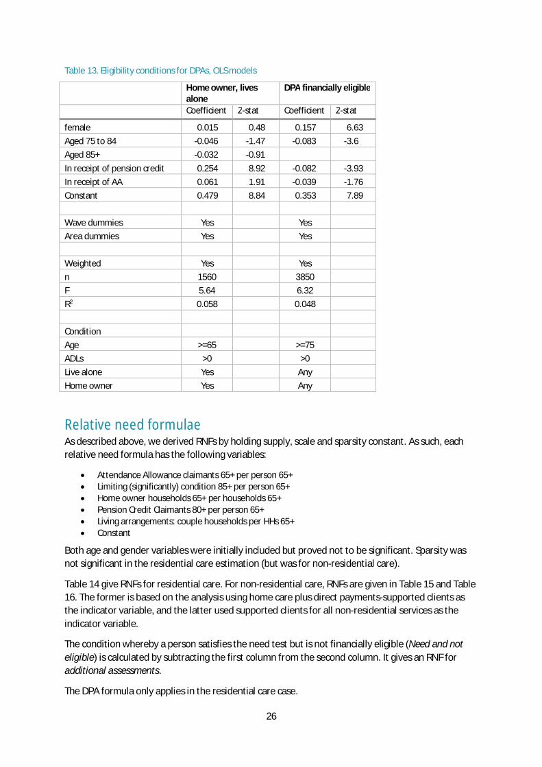
Table 13 gives the eligibility results as regards DPAs. As outlined above we used a model in ELSA to predict how the joint probability of being alone and a home owner varied with a number of need and wealth proxies (column 3). Conditional on being a home owner, living alone and in need, the risk factors for a person being financially eligible for a DPA were also modelled (column 2). As anticipated, people in this sub-group who were also pension credit recipients (compared to those not in receipt) were significantly more likely to qualify for a DPA in principle.

As above, these results were applied in the small areas models.

26

Table 13. Eligibility conditions for DPAs, OLS models

Home owner, lives alone

DPA financially eligible

Coefficient Z-stat Coefficient Z-stat

female 0.015 0.48 0.157 6.63 Aged 75 to 84 -0.046 -1.47 -0.083 -3.6 Aged 85+ -0.032 -0.91

In receipt of pension credit 0.254 8.92 -0.082 -3.93 In receipt of AA 0.061 1.91 -0.039 -1.76 Constant 0.479 8.84 0.353 7.89

Wave dummies Yes

Yes Area dummies Yes

Yes

Weighted Yes

Yes

n 1560

3850 F 5.64

6.32

R2 0.058

0.048

Condition Age >=65

>=75

ADLs >0

>0 Live alone Yes

Any

Home owner Yes

Any

Relative need formulae As described above, we derived RNFs by holding supply, scale and sparsity constant. As such, each relative need formula has the following variables:

Attendance Allowance claimants 65+ per person 65+ Limiting (significantly) condition 85+ per person 65+ Home owner households 65+ per households 65+ Pension Credit Claimants 80+ per person 65+ Living arrangements: couple households per HHs 65+ Constant

Both age and gender variables were initially included but proved not to be significant. Sparsity was not significant in the residential care estimation (but was for non-residential care).

Table 14 give RNFs for residential care. For non-residential care, RNFs are given in Table 15 and Table 16. The former is based on the analysis using home care plus direct payments-supported clients as the indicator variable, and the latter used supported clients for all non-residential services as the indicator variable.

The condition whereby a person satisfies the need test but is not financially eligible (Need and not eligible) is calculated by subtracting the first column from the second column. It gives an RNF for additional assessments.

The DPA formula only applies in the residential care case.

27

Table 14. Relative need formulae, residential care

Need + Elig (LA-

supported clients)

Need (All

clients)

Need and not

eligible

DPA

Attendance Allowance claimants 65+ per person 65+ 0.01213 0.02072 0.00858 0.00436 Limiting (significantly) condition 85+ per person 65+ 0.00736 0.01022 0.00286 0.00098 Home owner households 65+ per households 65+ -0.00244 0.00000 0.00244 0.00317 Pension Credit Claimants 80+ per person 65+ 0.01166 0.01552 0.00387 0.00331 Living arrangements: couple households per HHs 65+ -0.00377 -0.00735 -0.00358 -0.00598 Constant 0.00743 0.01012 0.00269 0.00169

Table 15. Relative need formulae, non-residential care (Home care + DP)


Need (All clients)

Need and not eligible

Attendance Allowance claimants 65+ per person 65+ 0.07983 0.09998 0.02014 Limiting (significantly) condition 85+ per person 65+ 0.20773 0.33162 0.12389 Home owner households 65+ per households 65+ -0.02195 0.00000 0.02194 Pension Credit Claimants 80+ per person 65+ 0.10760 0.07773 -0.02986 Living arrangements: couple households per HHs 65+ -0.03785 -0.04246 -0.00461 Constant 0.05288 0.05523 0.00235

Table 16. Relative need formulae, non-residential care (All NR services)


Need (All clients)

Need and not eligible

Attendance Allowance claimants 65+ per person 65+ 0.08339 0.11082 0.02744 Limiting (significantly) condition 85+ per person 65+ 0.13912 0.22154 0.08242 Home owner households 65+ per households 65+ -0.01681 0.00000 0.01681 Pension Credit Claimants 80+ per person 65+ 0.10011 0.08257 -0.01754 Living arrangements: couple households per HHs 65+ -0.03101 -0.03596 -0.00495 Constant 0.05025 0.05650 0.00625

To provide combined formulae (residential plus non-residential clients), we weighted the individual formulae together by the respective number of total supported clients in England for residential and non-residential services – see Table 17 based on the home care plus DP results, and Table 18 based on the results using all non-residential services. Note these are not cost-weighted and so favour the NR contribution, which has 418,000 clients versus 167,000 supported in residential care (2012/3).

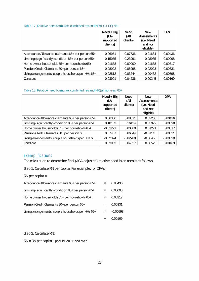
28

Table 17. Relative need formulae, combined res and NR (HC + DP) 65+

Need + Elig (LA-

supported clients)

Need (All

clients)

New Assessments

(i.e. Need and not eligible)

DPA


Table 18. Relative need formulae, combined res and NR (all non-res) 65+

Need + Elig (LA-

supported clients)

Need (All

clients)

New Assessments

(i.e. Need and not eligible)

DPA


Exemplifications The calculation to determine final (ACA-adjusted) relative need in an area is as follows:

Step 1. Calculate RN per capita. For example, for DPAs:

RN per capita =

Attendance Allowance claimants 65+ per person 65+ × 0.00436

Limiting (significantly) condition 85+ per person 65+ × 0.00098

Home owner households 65+ per households 65+ × 0.00317

Pension Credit Claimants 80+ per person 65+ × 0.00331

Living arrangements: couple households per HHs 65+ × -0.00598

+ 0.00169

Step 2. Calculate RN:

RN = RN per capita × population 65 and over

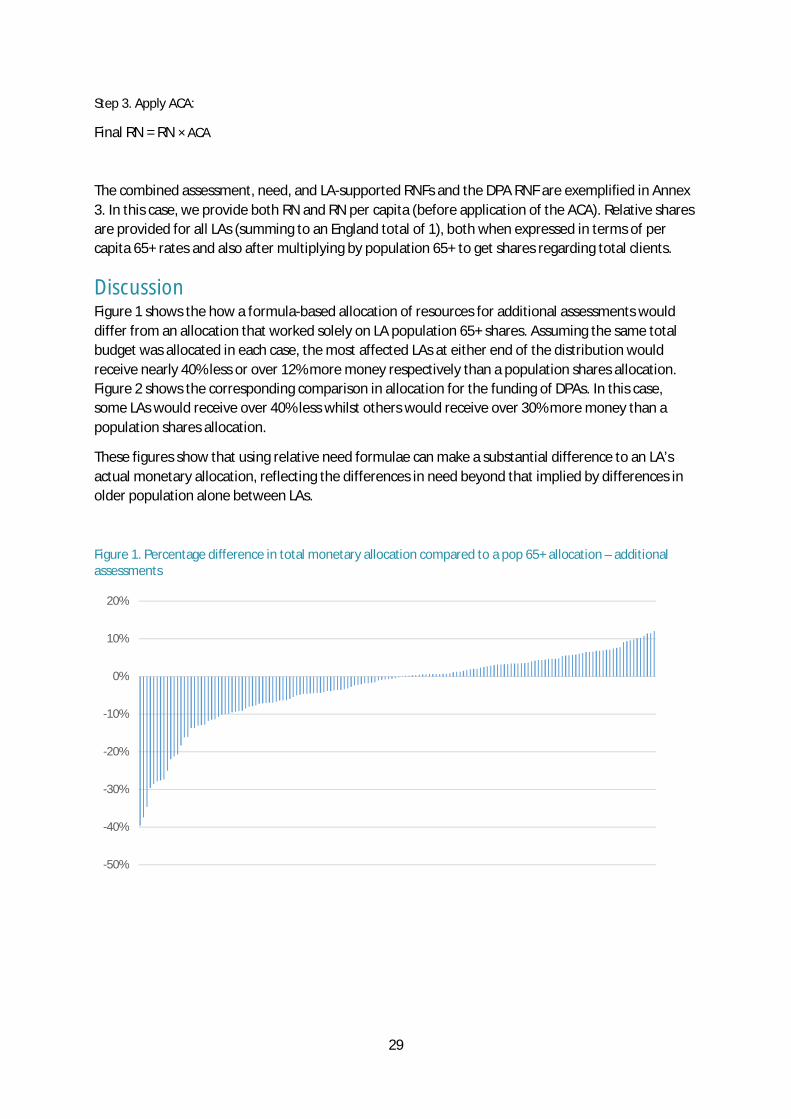
29

Step 3. Apply ACA:

Final RN = RN × ACA

The combined assessment, need, and LA-supported RNFs and the DPA RNF are exemplified in Annex 3. In this case, we provide both RN and RN per capita (before application of the ACA). Relative shares are provided for all LAs (summing to an England total of 1), both when expressed in terms of per capita 65+ rates and also after multiplying by population 65+ to get shares regarding total clients.

Discussion Figure 1 shows the how a formula-based allocation of resources for additional assessments would differ from an allocation that worked solely on LA population 65+ shares. Assuming the same total budget was allocated in each case, the most affected LAs at either end of the distribution would receive nearly 40% less or over 12% more money respectively than a population shares allocation. Figure 2 shows the corresponding comparison in allocation for the funding of DPAs. In this case, some LAs would receive over 40% less whilst others would receive over 30% more money than a population shares allocation.

These figures show that using relative need formulae can make a substantial difference to an LA’s actual monetary allocation, reflecting the differences in need beyond that implied by differences in older population alone between LAs.

Figure 1. Percentage difference in total monetary allocation compared to a pop 65+ allocation – additional assessments

-50%

-40%

-30%

-20%

-10%

0%

10%

20%

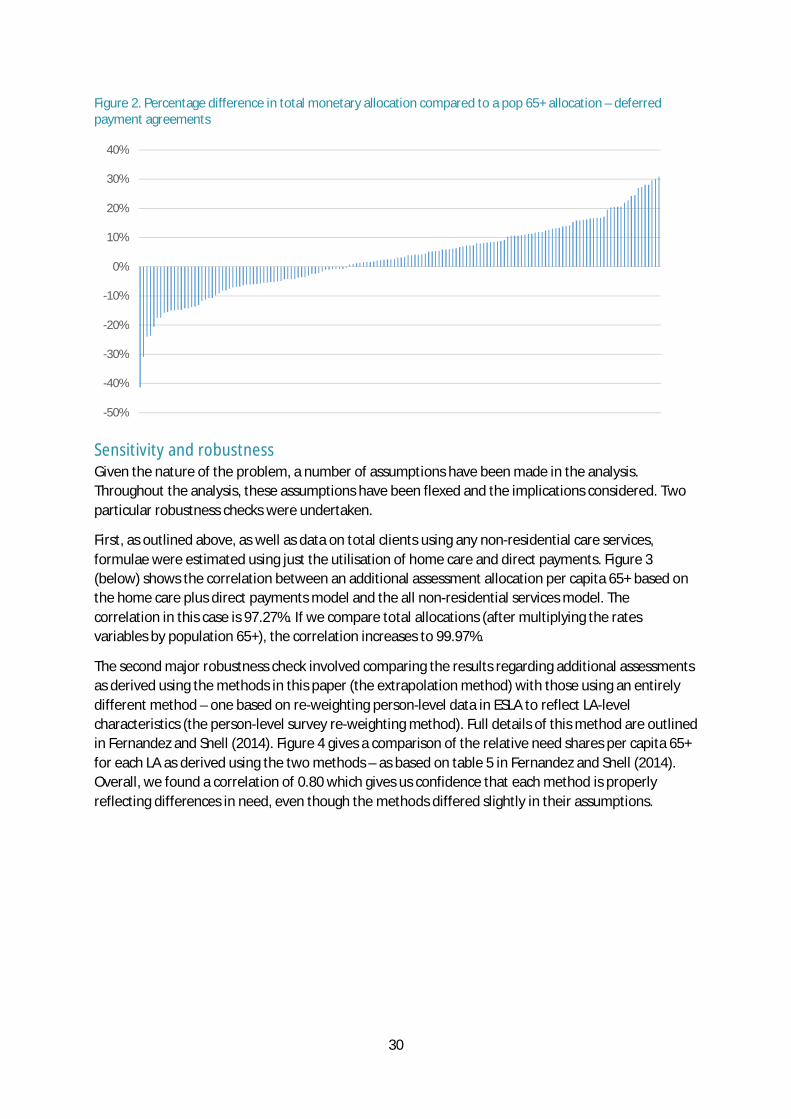
30

Figure 2. Percentage difference in total monetary allocation compared to a pop 65+ allocation – deferred payment agreements

Sensitivity and robustness Given the nature of the problem, a number of assumptions have been made in the analysis. Throughout the analysis, these assumptions have been flexed and the implications considered. Two particular robustness checks were undertaken.

First, as outlined above, as well as data on total clients using any non-residential care services, formulae were estimated using just the utilisation of home care and direct payments. Figure 3 (below) shows the correlation between an additional assessment allocation per capita 65+ based on the home care plus direct payments model and the all non-residential services model. The correlation in this case is 97.27%. If we compare total allocations (after multiplying the rates variables by population 65+), the correlation increases to 99.97%.

The second major robustness check involved comparing the results regarding additional assessments as derived using the methods in this paper (the extrapolation method) with those using an entirely different method – one based on re-weighting person-level data in ESLA to reflect LA-level characteristics (the person-level survey re-weighting method). Full details of this method are outlined in Fernandez and Snell (2014). Figure 4 gives a comparison of the relative need shares per capita 65+ for each LA as derived using the two methods – as based on table 5 in Fernandez and Snell (2014). Overall, we found a correlation of 0.80 which gives us confidence that each method is properly reflecting differences in need, even though the methods differed slightly in their assumptions.

-50%

-40%

-30%

-20%

-10%

0%

10%

20%

30%

40%

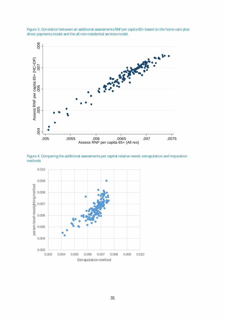
31

Figure 3. Correlation between an additional assessments RNF per capita 65+ based on the home care plus direct payments model and the all-non-residential services model.

Figure 4. Comparing the additional assessments per capital relative needs: extrapolation and imputation methods

.004

.005

.006

.007

.008

Asse

ss R

NF

per c

apita

65+

(HC

+DP)

.005 .0055 .006 .0065 .007 .0075Assess RNF per capita 65+ (All res)

0.003

0.004

0.005

0.006

0.007

0.008

0.009

0.010

0.003 0.004 0.005 0.006 0.007 0.008 0.009 0.010

pers

on-le

vel r

ewei

ghtin

g met

hod

Extrapolation method

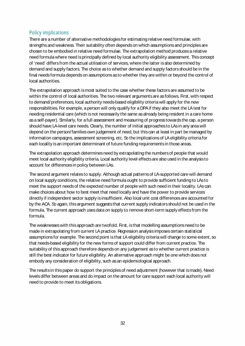
32

Policy implications There are a number of alternative methodologies for estimating relative need formulae, with strengths and weakness. Their suitability often depends on which assumptions and principles are chosen to be embodied in relative need formulae. The extrapolation method produces a relative need formula where need is principally defined by local authority eligibility assessment. This concept of ‘need’ differs from the actual utilisation of services, where the latter is also determined by demand and supply factors. The choice as to whether demand and supply factors should be in the final needs formula depends on assumptions as to whether they are within or beyond the control of local authorities.

The extrapolation approach is most suited to the case whether these factors are assumed to be within the control of local authorities. The two relevant arguments are as follows. First, with respect to demand/preferences, local authority needs-based eligibility criteria will apply for the new responsibilities. For example, a person will only qualify for a DPA if they also meet the LA test for needing residential care (which is not necessarily the same as already being resident in a care home as a self-payer). Similarly, for a full assessment and measuring of progress towards the cap, a person should have LA-level care needs. Clearly, the number of initial approaches to LAs in any area will depend on the person/families own judgement of need, but this can at least in part be managed by information campaigns, assessment screening, etc. So the implications of LA eligibility criteria for each locality is an important determinant of future funding requirements in those areas.

The extrapolation approach determines need by extrapolating the numbers of people that would meet local authority eligibility criteria. Local authority level effects are also used in the analysis to account for differences in policy between LAs.

The second argument relates to supply. Although actual patterns of LA-supported care will demand on local supply conditions, the relative need formula ought to provide sufficient funding to LAs to meet the support needs of the expected number of people with such need in their locality. LAs can make choices about how to best meet that need locally and have the power to provide services directly if independent sector supply is insufficient. Also local unit cost differences are accounted for by the ACA. So again, this argument suggests that current supply indicators should not be used in the formula. The current approach uses data on supply to remove short-term supply effects from the formula.

The weaknesses with this approach are twofold. First, is that modelling assumptions need to be made in extrapolating from current LA practice. Regression analysis imposes certain statistical assumptions for example. The second point is that LA eligibility criteria will change to some extent, so that needs-based eligibility for the new forms of support could differ from current practice. The suitability of this approach therefore depends on any judgement as to whether current practice is still the best indicator for future eligibility. An alternative approach might be one which does not embody any consideration of eligibility, such as an epidemiological approach.

The results in this paper do support the principles of need adjustment (however that is made). Need levels differ between areas and do impact on the amount for care support each local authority will need to provide to meet its obligations.

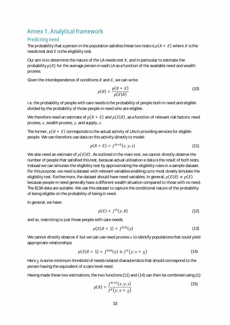
33

Annex 1. Analytical framework Predicting need The probability that a person in the population satisfies these two tests is 푝(푅 + 퐸) where 푅 is the needs test and 퐸 is the eligibility test.

Our aim is to determine the nature of the LA needs test 푅, and in particular to estimate the probability 푝(푅) for the average person in each LA as a function of the available need and wealth proxies.

Given the interdependence of conditions 푅 and 퐸, we can write:

푝(푅) =

푝(푅 + 퐸)푝(퐸|푅)

(10)

i.e. the probability of people with care needs is the probability of people both in need and eligible divided by the probability of those people in need who are eligible.

We therefore need an estimate of 푝(푅 + 퐸) and 푝(퐸|푅), as a function of relevant risk factors: need proxies, 푥, wealth proxies, 푦, and supply, 푠.

The former, 푝(푅 + 퐸) corresponds to the actual activity of LAs in providing services for eligible people. We can therefore use data on this activity directly to model:

푝(푅 + 퐸) = 푓 (푥,푦, 푠) (11)

We also need an estimate of 푝(퐸|푅). As outlined in the main text, we cannot directly observe the number of people that satisfied this test, because actual utilisation e data is the result of both tests. Instead we can simulate the eligibility test by approximating the eligibility rules in a sample dataset. For this purpose, we need a dataset with relevant variables enabling us to most closely simulate the eligibility test. Furthermore, the dataset should have need variables. In general, 푝(퐸|푅) ≠ 푝(퐸) because people in need generally have a different wealth situation compared to those with no need. The ELSA data are suitable. We use this dataset to capture the conditional nature of the probability of being eligible on the probability of being in need.

In general, we have:

푝(퐸) = 푓 (푦;푅) (12)

and so, restricting to just those people with care needs:

푝(퐸|푅 = 1) = 푓 | (푦) (13)

We cannot directly observe 푅 but we can use need proxies 푥 to identify populations that could yield appropriate relationships:

푝(퐸|푅 = 1) = 푓 | (푦) ≅ 푓 푦; 푥 > 푥 (14)

Here 푥 is some minimum threshold of needs-related characteristics that should correspond to the person having the equivalent of a care level need.

Having made these two estimations, the two functions (11) and (14) can then be combined using (1):

푝(푅) =

푓 (푥,푦, 푠)푓 푦; 푥 > 푥

(15)

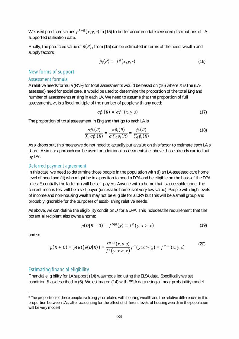
34

We used predicted values 푓 (푥, 푦, 푠) in (15) to better accommodate censored distributions of LA-supported utilisation data.

Finally, the predicted value of 푝̂(푅) from (15) can be estimated in terms of the need, wealth and supply factors:

푝̂ (푅) = 푓 (푥,푦, 푠) (16)

New forms of support Assessment formula A relative needs formula (RNF) for total assessments would be based on (16) where 푅 is the (LA-assessed) need for social care. It would be used to determine the proportion of the total England number of assessments arising in each LA. We need to assume that the proportion of full assessments, 휎, is a fixed multiple of the number of people with any need:

휎푝̂ (푅) = 휎푓 (푥,푦, 푠) (17)

The proportion of total assessment in England that go to each LA is:

휎푝̂ (푅)∑ 휎푝̂ (푅) =

휎푝̂ (푅)휎∑ 푝̂ (푅) =

푝̂ (푅)∑ 푝̂ (푅)

(18)

As 휎 drops out, this means we do not need to actually put a value on this factor to estimate each LA’s share. A similar approach can be used for additional assessments i.e. above those already carried out by LAs.

Deferred payment agreement In this case, we need to determine those people in the population with (i) an LA-assessed care home level of need and (ii) who might be in a position to need a DPA and be eligible on the basis of the DPA rules. Essentially the latter (ii) will be self-payers. Anyone with a home that is assessable under the current means-test will be a self-payer (unless the home is of very low value). People with high levels of income and non-housing wealth may not be eligible for a DPA but this will be a small group and probably ignorable for the purposes of establishing relative needs.5

As above, we can define the eligibility condition 퐷 for a DPA. This includes the requirement that the potential recipient also owns a home:

푝(퐷|푅 = 1) = 푓 | (푦) ≅ 푓 푦;푥 > 푥 (19)

and so

푝(푅 + 퐷) = 푝(푅) 푝(퐷|푅) =

푓 (푥,푦, 푠)푓 푦; 푥 > 푥

푓 푦;푥 > 푥 = 푓 (푥,푦, 푠) (20)

Estimating financial eligibility Financial eligibility for LA support (14) was modelled using the ELSA data. Specifically we set condition 퐸 as described in (6). We estimated (14) with ESLA data using a linear probability model

5 The proportion of these people is strongly correlated with housing wealth and the relative differences in this proportion between LAs, after accounting for the effect of different levels of housing wealth in the population will be very modest.

35

(OLS) over a sub-sample of people with at least one ADL, a proxy for the 푅 = 1 condition in (14). Both need and wealth factors were used in the estimation:

퐸(푅 = 푥 ) = 훽 + 훽 푥 + 훽 푦 + 휖 (21)

The independent variables are described in the main text.

Financial eligibility for a DPA was also simulated in ELSA using the rules outlined above (8). We estimated this model in two parts.

푝(퐷|푅 = 1) = 푝(표푤푛,푎푙표푛푒,푛푒푒푑) × 푝(푁퐻푊 < 23250)= 푓 (푥 ,푦 )푓 | 푥 | ,푦 |

(22)

The two functions 푓 and 푓 | were also estimated using linear (OLS) probability models.

Estimating need eligibility The discussion of the analytical framework above refers to individual person probabilities. But this analysis readily generalises to the population level (e.g. an LSOA). This generalisation is achieved by calculating the expected number of people in a population that would satisfy the relevant conditions.

Suppose there are 푗 people in each LSOA 푖, then (1) can be written:

푝 (푅 + 퐸) = 푝 (푅)푝 (퐸|푅) (23)

We do not observe 푝 (퐸|푅) at LSOA level but rather use an individual level estimate from elsewhere (using ELSA data, see below) and assume that 푝 (퐸|푅) = 푝 (퐸|푅), the mean value for the LOSA. As such, (23) becomes:

푐 = 푝 (퐸|푅) 푝 (푅) = 푝 (퐸|푅)푐 (24)

where 푐 is the count of people satisfying the needs and eligibility tests. Also, 푐 is the count of people satisfying just the need test. A similar function can be written for the DPA test:

푐 = 푝 (퐷|푅)푐 (25)

In generalising in this way, we need to assume that individual level probabilities in a given small area population are about the same. This assumption seems reasonable if the relevant characteristics of people in that population are also similar. For this reason, we use as small a population level as possible for the analysis; namely LSOA populations.

We estimated a number of RNFs, for different conditions. As a shorthand, we use the variable 푔 to summarise the relevant condition: 푔 = {푅 + 퐸,푅,푅 + 퐷}.

The general method used involves calculating the expected counts of people in each LSOA who satisfy condition 푔 and then using a regression model to estimate a prediction formula for these numbers based on LSOA population rates of relevant need, wealth and supply factors.

We fit count models to the small area data:

푐 = exp 훽 + 훽

푧푚

+ 훽 ln(푚 ) (26)

36

at the LSOA 푖 level. Here 푐 is the count of recipients per LSOA satisfying condition 푔 = {푅 +퐸,푅,푅 + 퐷}. Also, 푧 are both the need and wealth variables and 푚 is the over 65s’ population of the LSOA.

The inclusion of a population size variable in an LSOA-level analysis is mainly to account for scale effects. Other things equal, the numbers of clients in any area should be proportional to the population in that area.

We could estimate a model in rates of service users per capita (65+) but count models should be better able to deal with integer effects in small areas by having population on the right-hand side. We only observe integer counts of service users by LSOA in the data, noting that the average number of clients in any LSOAs is unlikely to be an integer. Consequently in small LSOAs we might observe zero clients even if the average is greater than zero (but less than one). Similarly, in larger LSOAs we are more likely to see positive integer numbers of clients, whereas the average is less than this amount. Consequently, the size of the LSOA can artificially affect the actual observed numbers of clients, and we need to control for this artefact in the analysis.

A standard set of variables, 푧 , were included in each estimation (of the different 푔’s), grouped by primary variable type: need, wealth and supply. These are described in the main text.

Linear formulae A linear approximation can be obtained using a first-order Taylor Series expansion of (26):

푐 ≅ 휋 + 휋 (푚 )

푧푚

+ 휋 (푚 )푚 (27)

where 휋 = and 휋 = are coefficients of a linear formula.

This formula can be summed to the LA level.

푐 ≅ 푁 휋 + 휋

푧푚

+⋯+ 휋푧푚

+ 휋 푚 (28)

This can be further simplified is we assume that the linear coefficients are not functions of population and therefore constant for each LSOA 푖. We explore this assumption below. This means:

퐶 ≅ 푁 휋 + 휋

푧푚

+ ⋯+ 휋푧푚

+ 휋 푚 (29)

The 푧 terms are needs factors and these may be assumed to apply at the person level and not functions of the size of local populations, i.e.

푧 = 휙 푚 (30)

Consequently, ∑ = ∑ 휙 = 푁 휙 = 푁 , where 푍 = ∑ 푧 is the LA sum of the need factor

e.g. number of people claiming AA, and 푀 = ∑ 푚 the LA-level population 65+.

Using this result in (29) gives:

퐶 ≅ 푁 휋 + 휋 푁

푍푀

+⋯+ 휋 푁푍푀

+ 휋 푀 (31)

37

Or

퐶푀

≅푁푀

휋 + 휋푁푀

푍푀

+ ⋯+ 휋푁푀

푍푀

+ 휋 (32)

Finally, average LOSA population 65+ in LA 푙 is 푚 = 푀 /푁 and therefore:

퐶푀

≅휋푚

+ 휋 +휋푚

푍푀

+⋯+휋푚

푍푀

(33)

This method can be applied to any condition 푔 and therefore we can write the general case as:

퐶푀

≅ 훼 + 훼푍푀

+⋯+ 훼푍푀

(34)

where 훼 = and 훼 = + 휋 .

In theory, the 훼’ are functions of population size, 푚 , and therefore subject to scaling issues. Local authorities with different populations would have different coefficients. In practice, we might expect client counts to be directly proportional to LSOA population size, after accounting for any integer effects. In this case, we would expect that the coefficient 훽 to have a value close to one. We have:

훼 =

휋푚

=1푚

휕푐

휕푧푚

=훽푚

exp 훽 + 훽푧푚

exp 훽 푙푛(푚 )

= 훽 exp 훽 + 훽 휙 푚

(35)

Consequently if 훽 = 1, then 훼 = 훽 exp 훽 + ∑ 훽 휙 , that is, not a function of 푚 . We tested this assumption directly using the estimated value of 훽 in the empirical analysis.

Annex 2. Data sources and manipulation Population Estimates at July 2012 Source: We used mid-2012 population estimates for Lower Layer Super Output Areas 2011 by single year of age and sex, as they are the closest population estimates available to February 2013 (i.e., the month and year for the rest of statistics used in the analysis). The statistics are provided by the Office of National Statistics, Population Statistics Division.6

Manipulation: Using these statistics we computed through aggregation of single years of age and/or gender various population groups at LSOA 2011 level: total population, population aged 60 and over, population aged 65 and over, female population aged 65 and over, population aged 70 and over, and working age population (i.e., aged 16 to 64). Figure 5 presents the distribution of the population 65 and over at local authority level – this varied considerably, with the largest population 65 and over exceeding 250,000 (in Kent, Essex and Hampshire) and the smallest being 545 (Isles of Silly) and 1,106 (City of London).

6 http://www.ons.gov.uk/ons/publications/re-reference-tables.html?edition=tcm%3A77-320861

38

Benefits Claimants Data Source: We used data on counts of benefits claimants at February 2013 (i.e., Attendance Allowance, Disability Living Allowance, Employment and Support Allowance, Income Support, Jobseekers Allowance and Pension Credit claimants) provided by the Department for Work and Pensions.7 The statistics are at 2001 Lower Layer Super Output Area (LSOA).

Manipulation: As the analysis is performed at 2011 LSOA level, we matched 2001 to 2011 LSOAs by using the “Lower Layer Super Output Area 2001 to Lower Layer Super Output Area 2011 E+W Lookup” provided by the UK Data Service Census Support.8 For LSOAs 2011 that resulted from a merge of two or more LSOAs 2001 (i.e., 145 LSOAs 2011), the count of benefits claimants was computed as the sum of benefits claimants from the respective LSOAs 2001. For LSOAs 2011 that resulted from a split of a LSOA 2001 (i.e. 881 LSOAs 2011), the count of benefits claimants was estimated as a share of benefits claimants from the respective LSOA 2001. The shares are based on the population living in a LSOA 2011 that resulted from a split divided by the sum of populations living in all LSOAs 2011 that resulted from that particular split. We used different population groups to compute the population shares for the various types of benefit claimants:

1. for Attendance Allowance claimants we used the population aged 65 and over; 2. for Disability Living Allowance claimants - the total population; 3. for Employment and Support Allowance, Income Support, Jobseekers Allowance claimants -

the working age population (i.e., aged 16 to 64); 4. for Pension Credit claimants - the population 60 and over; while 5. for Disability Living Allowance and Pension Credit claimants aged 70 and over - the

population aged 70 and over.

We could not estimate the count of benefit claimants for 146 LSOAs 2011 that resulted from a mix of merges and splits of LSOAs 2001. For these LSOAs, the values for the count of benefit claimants are set as missing.

Figures 6 and 7 illustrate the distribution by upper tier local authority of shares of Attendance Allowance claimants aged 65 and over and Pension Credit claimants aged 80 and over in the population 65 and over.9 While the distribution of the count of Attendance Allowance claimants aged 65 and over and Pension Credit claimants aged 80 and over resembles that of the population 65 and over, the shares in the population 65 and over serve as a proxy for relative deprivation that is likely to be highly correlated with relative needs. The share of Attendance Allowance claimants aged 65 and over in the population 65 and over ranges from over 0.22 (in the case of Sandwell and Tower Hamlets) to about 0.10 (in the case of the City of London and Wokingham). Similarly, the share of Pension Credit claimants aged 80 and over in the population 65 and over ranges from 0.16 (Tower Hamlets) and 0.14 (Sandwell) to 0.04 (City of London and Wokingham).

Number of Care Home Beds Source: Data on the number of care home beds and type of clients at February 2013 were extracted from the Care Directory statistics provided by the Care Quality Commission.10 The statistics are at care home level.

7 http://tabulation-tool.dwp.gov.uk/NESS/BEN/iben.htm 8 http://ukbsrv-at.edina.ac.uk/html/lut_download/lut_download.html?data=lsoa01_lsoa11_ew_lu 9 The aggregation at upper tier LA has been made directly from the original statistics at LSOA 2001 level. Therefore, it includes also the benefit claimants we could not assign to the 146 LSOAs 2011. 10 http://www.cqc.org.uk/cqcdata

39

Manipulation: Before estimating the number of care home beds at LSOA 2011 level, we cleaned the data by dropping duplicated care homes (24 care homes),11 corrected typos in the care home postal codes (1 care home), corrected the entry for Local Authority Area (10 care homes) and replaced missing values for Service User Band (i.e., type of client) using information from carehome.co.uk (7 care homes).

The number of care home beds for “Old Age/Dementia” clients at LSOA 2011 level was estimated in two steps. In the first step, the number of care home beds of the care homes that registered to serve either “Old Age” or “Dementia” clients or both was aggregated at postal code level. Then, using the November 2013 Office for National Statistics Postcode Directory Open Edition,12 postcodes were matched to LSOAs 2011. In the second step, the care home bed numbers for “Old Age/Dementia” clients at postal code level were aggregated at LSOA 2011 level.

The “Number of care home beds for old age and dementia” is a measure of care supply. Not surprisingly the highest number of care home beds are found in areas with the largest population 65 and over, as the demand for care is higher; the correlation between the “Number of care home beds for old age and dementia at LA level” and “Population 65 and over at LA level” is 0.983. However, due to cost reasons, the highest concentration of care home beds for old age and dementia in the population 65 and over is in areas with relatively lower house prices: the highest concentration is for example in Middleborough (0.073), Torbay (0.069) and Bournemouth (0.068), while the lowest concentration is in the City of London (nil) and London boroughs (e.g., Hackney [0.014], Westminster [0.015] and Camden [0.021]; see Figure 8).

Residential Care Clients aged 65 and over Source: Statistics at LSOA level on the Number of Local Authority (LA) Supported Permanent Admissions to Residential and Nursing Care during 1 April 2012 and 31 March 2013 were collected by LG Futures from 60 sampled Local Authorities (see Table 19; for more details see LG Futures (2014) Report on Engagement and Data Collection Activities). Two datasets were created: the first on the basis of clients’ pre-care address, while the second on clients’ care address. Both include the count of clients by six primary client types (i.e., Physical Disability, Mental Health, Learning Disability, Substance Misuse and Other Vulnerable People, and Not Allocated) and three types of residence (i.e., LA Staffed Residential Care, Independent Residential Care, and Nursing Care). Values at LSOA level of “1”, “2”, “3”, and “4” were masked by Local Authorities (i.e., replaced by “*”), as this data has been classified as personal identifiable.

From the 60 sampled LAs, three submitted incomplete data (i.e., Birmingham, Peterborough and Sutton), while four were excluded (i.e., Bexley, Croydon, Hounslow and Enfield) as aggregated totals could not be validated when compared to national returns from the Community Care Statistics, Social Services Activity, England - 2012-13, Final release [NS], reported by the Health and Social Care Information Centre.13 The final sample included 53 Local Authorities, covering 14,003 LSOAs.

Manipulation: For each type of residence, we replaced missing values for Total Primary Clients with the sum of values for the respective primary client types. In total, 14 missing values were replaced for LA Staffed Residential Care, 60 missing values were replaced for Independent Residential Care, and 45 missing values were replaced for Nursing Care. Moreover, zero values of Total Primary Clients were replaced with the sum of values for the respective primary client types if at least one of

11 Double entries in the Care Home register are sometimes due to a change in management. 12 http://ukbsrv-at.edina.ac.uk/html/pcluts_download/pcluts_download.html?data=pcluts_2013nov 13 http://www.hscic.gov.uk/catalogue/PUB13148/comm-care-stat-act-eng-2012-13-fin-data.zip

40

the latter values was different from zero: 19 zero values were replaced for LA Staffed Residential Care, 88 zero values were replaced for Independent Residential Care, and 195 zero values were replaced for Nursing Care.

For Total Primary Clients in Residential Care (i.e., LA Staffed Residential Care + Independent Residential Care) and Total Primary Clients in Nursing Care, we replaced masked values (i.e., “*”) with “*” mean values computed at LA level. The “*” mean value for residential care for LA i (∗ ) is computed as:

∗ =푁푅푅푒푠퐶푎푟푒 − ∑ 푅푒푠퐶푎푟푒

푁∗ ,∀ 푅푒푠퐶푎푟푒 ≥ 5

where 푁푅푅푒푠퐶푎푟푒 stands for National Return of Total Primary Client Types in Residential Care in the LA i, 푅푒푠퐶푎푟푒 stands for Total Primary Client Types in Residential Care in LA i and LSOA j, and 푁∗ represents the total number of “*” values for residential care clients in the LA i.

The “*” mean value for nursing care for LA i (∗ ) is computed as:

∗ =푁푅푁푢푟퐶푎푟푒 − ∑ 푁푢푟퐶푎푟푒

푁∗ ,∀ 푁푢푟퐶푎푟푒 ≥ 5

where 푁푅푁푢푟퐶푎푟푒 stands for National Return of Total Primary Client Types in Nursing Care in the LA i, 푁푢푟퐶푎푟푒 stands for Total Primary Client Types in Nursing Care in LA i and LSOA j, and 푁∗ represents the total number of “*” values for nursing care clients in the LA i.

In order to remove outliers from both ∗ and ∗ , values smaller than the 5th percentile weighted by the number of stars at LA level (i.e., 푁∗ and 푁∗ respectively) were replaced with the 5th weighted percentile value. Similarly, values higher than the 95th weighted percentile were replaced with the 95th weighted percentile value. The ∗ and ∗ values used to replace the masked values are presented in Table 20, along with the estimated number of LA supported permanent admissions to residential and nursing care at upper tier LA level. The estimates were obtained through the aggregation of the LSOA level data after replacing the masked values.

After replacing the masked values, the variables Total Primary Clients in Residential Care and Total Primary Clients in Nursing Care were used to compute Gross Weekly Residential Care Expenditures at LSOA level. As local unit cost can be influenced by differences in the commissioning practices of councils, national average unit costs were applied. The unit cost figures in Table 21 were taken from the Personal Social Services Expenditure and Unit Costs - England, 2012-13, Final release [NS] reported by the Health and Social Care Information Centre.14 The cost-weighted Gross Weekly Residential Care Expenditures for each LSOA k (퐺푊푅푒푠퐶푎푟푒퐸푥푝 ) are:

퐺푊푅푒푠퐶푎푟푒퐸푥푝 = 528.40 × 푅푒푠퐶푎푟푒 + 507.40 × 푁푢푟퐶푎푟푒

Non-residential Care Clients aged 65 and over Source: Statistics at LSOA level on Number of Clients Registered to Receive Community Based Services Provided or Commissioned by the CASSR on 31 March 2013 by primary client type and components of service were collected by LG Futures from 60 sampled Local Authorities (see Table 22; for more details see LG Futures (2014) Report on Engagement and Data Collection Activities). Four LAs (i.e., Hammersmith and Fulham, Peterborough, St. Helens and Suffolk) could not submit all the data required and were not used in the analysis, while data from seven further LAs were

14 http://www.hscic.gov.uk/catalogue/PUB13085

41

excluded due to apparent inconsistencies between counts of clients at LA level and RAP returns (i.e., Bexley, Cambridgeshire, Coventry, Croydon, Enfield, Hounslow, and Kensington and Chelsea). The dataset included counts by five primary client types (i.e., Physical Disability, Mental Health, Learning Disability, Substance Misuse, and Other Vulnerable People), eight components of service (i.e., Home Care, Day Care, Meals, Short-Term Residential Not Respite, Direct Payments, Professional Support, Equipment and Adaptions, and Other) and the Total of Clients. Values at LSOA level of “1”, “2”, “3”, and “4” were masked by Local Authorities (i.e., replaced by “*”), as this data has been classified as personal identifiable.

Manipulation: Three components of service were used for the estimation of the Relative Needs Formulae: Total of Clients, Home Care, and Direct Payments. For each of these components, we first replaced missing values of total primary client types with the sum of values for the respective primary client types. In total, 83 missing values were replaced for Total of Clients, 82 missing values were replaced for Home Care, and 35 missing values were replaced for Direct Payments. Moreover, zero values of total primary client types were replaced with the sum of values for the respective primary client types if at least one of the latter values was different from zero. In total, 13 zero values were replaced for Total of Clients, 206 zero values were replaced for Home Care, and 200 zero values were replaced for Direct Payments.

The masked values (i.e., “*”) were replaced with “*” mean values computed at LA level. The “*” mean value for Total of Clients for LA i (∗ ) was computed as:

∗ =푅퐴푃푇표푡퐶푙푖푒푛푡 − ∑ 푇표푡퐶푙푖푒푛푡

푁∗ ,∀ 푇표푡퐶푙푖푒푛푡 ≥ 5

where 푅퐴푃푇표푡퐶푙푖푒푛푡 stands for RAP Return of Total of Non-Residential Clients in the LA i, 푇표푡퐶푙푖푒푛푡 stands for Total of Non-Residential Clients in LA i and LSOA j, and 푁∗ represents the total number of “*” values for the Total of Non-Residential Clients in the LA i.

The “*” mean value for Home Care for LA i (∗ ) is computed as:

∗ =푅퐴푃퐻표푚퐶푎푟푒 − ∑ 퐻표푚퐶푎푟푒

푁∗ ,∀ 퐻표푚퐶푎푟푒 ≥ 5

where 푅퐴푃퐻표푚퐶푎푟푒 stands for RAP Return of Non-Residential Clients Receiving Home Care in the LA i, 퐻표푚퐶푎푟푒 stands for Non-Residential Clients Receiving Home Care in the LA i and LSOA j, and 푁∗ represents the number of “*” values for non-residential clients receiving home care in the LA i.

The “*” mean value for Direct Payments for LA i (∗ ) was computed as:

∗ =푅퐴푃퐷푖푟푃푎푦 − ∑ 퐷푖푟푃푎푦

푁∗ ,∀ 퐷푖푟푃푎푦 ) ≥ 5

where 푅퐴푃퐷푖푟푃푎푦 stands for RAP Return of Non-Residential Clients Receiving Direct Payments in the LA i, 퐷푖푟푃푎푦 stands for Non-Residential Clients Receiving Direct Payments in the LA i and LSOA j, and 푁∗ represents the number of “*” values for non-residential clients receiving direct payments in the LA i.

For both ∗ , ∗ and ∗ , values that were out of the [0,5] range were dropped, as in this case aggregated LA data were considered to differ significantly from RAP returns: values for 29 LAs had to be dropped from ∗ as well as values for 8 LAs from the ∗ and ∗ . From the remaining, values smaller than the 5th percentile weighted by the number of stars at LA level (i.e., 푁∗ ,푁∗ and 푁∗

42

respectively) were replaced with the 5th weighted percentile value. Similarly, values higher than the 95th weighted percentile were replaced with the 95th weighted percentile value. The final ∗ , ∗ and ∗ values used to replace the masked values for Total of Non-Residential Care Clients, Home Care Clients and Direct Payments Clients are presented in Table 23. The second part of Table 23 presents the estimated number of clients registered to receive community based services at upper tier LA level. The estimates were obtained through the aggregation of the LSOA level data after replacing the masked values.

After replacing the masked values, the variables Home Care Clients in Direct Payments Clients were used to estimate Gross Weekly Non-Residential Care Expenditures at LSOA level. As local unit cost can be influenced by differences in the commissioning practices of councils, national average unit costs were applied. The unit cost figures were taken from the Personal Social Services Expenditure and Unit Costs - England, 2012-13, Final release [NS] reported by the Health and Social Care Information Centre.15 The cost-weighted Gross Weekly Non-Residential Care Expenditures for each LSOA k (퐺푊푁표푛푅푒푠퐶푎푟푒퐸푥푝 ) are:

퐺푊푁표푛푅푒푠퐶푎푟푒퐸푥푝 = 187.50 × 퐻표푚퐶푎푟푒 + 172.90 × 퐷푖푟푃푎푦

The cost-weighted gross weekly residential and non-residential care expenditures for the sampled LAs are presented in Table 24.

Census 2011 data We used Census 2011 data at LSOA level for specific indicators of needs, wealth and sparsity:

Count of people aged 85 and over with substantial activities of daily life limitations (i.e., day-to-day activities limited a lot) at LSOA level – Census 2011 Table ID LC3302EW;16

Count of households with members living as a couple (i.e., married or cohabiting) aged 65 and over at LSOA level – Census 2011 Table ID LC1102EW; 17

Count of homeowner households (i.e., home owned outright) aged 65 and over at LSOA level – Census 2011 Table ID LC4201EW;18

Count of households with members aged 65 and over at LSOA level – Census 2011 Table ID LC4201EW;

LSOA area (in hectares) – Census 2011 Table ID QS102EW; 19 We used the share of homeowner households aged 65 and over in the total number households 65 and over as a measure of housing wealth. As illustrated by Figure 9, housing wealth is quite unevenly distributed, ranging from over 0.75 in Wokingham, South Gloucestershire, Havering, and Solihull to about 0.20 in the London boroughs of Hackney and Tower Hamlets. The share of couples aged 65 and over in the total number of households 65 and over offers an alternative indicator of needs, as couples may help each other in time need and access less LA care support. Again we find quite a lot of variation (see Figure 10), with LAs like Wokingham, Rutland, East Riding of Yorkshire, Isles of Scilly, Lincolnshire, South Gloucestershire and Dorset having more than 50 per cent of households 65 and over living as couples, while only about 25 per cent of households over 65 live as couples in the London boroughs of Hackney, Islington, Hammersmith and Fulham, and Lambeth.

15 http://www.hscic.gov.uk/catalogue/PUB13085 16 https://www.nomisweb.co.uk/census/2011/lc3302ew 17 https://www.nomisweb.co.uk/census/2011/lc1102ew 18 https://www.nomisweb.co.uk/census/2011/lc4201ew 19 https://www.nomisweb.co.uk/census/2011/qs102ew

43

English Longitudinal Study of Ageing data The English Longitudinal Study of Ageing (ELSA) began in 2002 drawing on the sample of individuals aged 50 and over from the Health Survey of England (1998, 1999, 2001). ELSA collects large amount of data on the individual and family circumstances and quality of life among older people. It explores the dynamic relationships between health and functioning, social networks and participation, and economic position of people during the pre-retirement period and after retirement.

We used ELSA data to estimate the number of individuals financially eligible under the new Care Bill for local authority social care support and Deferred Payment Arrangements. This data set provides a range of sound financial variables which are not routinely available at the regional level, but which determine eligibility. These data were used to model financial and DPA eligibility as outlined in the main text. The models included, variously, the respondent’s sex, age group and number of activities of daily life (ADL) limitations; indicators for living alone, owning the accommodation (outright), receiving pension credit and receiving attendance allowance; and wave and regional controls. Summary statistics of these variables are presented in Table 25.

44

Table 19. Sampled Local Authorities – Residential Care

LA code LA name LA code LA name

E06000055 Bedford E08000034 Kirklees

E09000004 Bexleyb E10000017 Lancashire

E08000025 Birminghama E06000016 Leicester

E06000009 Blackpool E10000019 Lincolnshire

E06000036 Bracknell Forest E08000003 Manchester

E09000006 Bromley E09000024 Merton

E10000002 Buckinghamshire E06000042 Milton Keynes

E10000003 Cambridgeshire E06000024 North Somerset

E09000007 Camden E06000048 Northumberland

E06000049 Cheshire East E10000024 Nottinghamshire

E06000052 Cornwall E10000025 Oxfordshire

E06000047 County Durham E06000031 Peterborougha

E08000026 Coventry E06000038 Reading

E09000008 Croydonb E08000005 Rochdale

E10000007 Derbyshire E08000028 Sandwell

E09000009 Ealing E08000014 Sefton

E10000011 East Sussex E08000029 Solihull

E09000010 Enfieldb E08000013 St Helens

E10000012 Essex E08000007 Stockport

E10000013 Gloucestershire E10000029 Suffolk

E09000012 Hackney E10000030 Surrey

E09000013 Hammersmith and Fulham E09000029 Suttona

E10000014 Hampshire E06000030 Swindon

E09000014 Haringey E06000027 Torbay

E06000001 Hartlepool E09000030 Tower Hamlets

E09000017 Hillingdon E09000031 Waltham Forest

E09000018 Hounslowb E09000033 Westminster

E06000046 Isle of Wight E06000054 Wiltshire

E09000020 Kensington and Chelsea E08000031 Wolverhampton

E10000016 Kent E06000014 York Notes: a Excluded due to incomplete data submitted. b Excluded due to inconsistencies between aggregated totals and national returns.

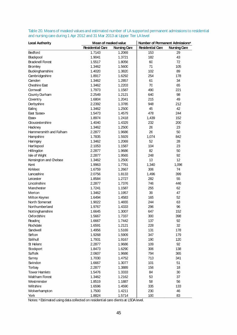
45

Table 20. Means of masked values and estimated number of LA supported permanent admissions to residential and nursing care during 1 Apr 2012 and 31 Mar 2013 at Upper Tier LA level

Local Authority Mean of masked value Number of Permanent Admissionsa

Residential Care Nursing Care Residential Care Nursing Care Bedford 1.7143 1.2069 153 29 Blackpool 1.9041 1.3721 182 43 Bracknell Forest 1.5517 1.8056 60 72 Bromley 1.3462 1.5600 71 105 Buckinghamshire 1.4020 1.3820 102 89 Cambridgeshire 1.8917 1.6292 254 178 Camden 1.3462 1.2857 61 34 Cheshire East 1.3462 1.2203 70 65 Cornwall 1.7973 1.1587 490 221 County Durham 2.2549 1.2121 640 98 Coventry 1.6804 1.2041 215 49 Derbyshire 2.2392 1.3785 948 212 Ealing 1.3462 1.2500 45 42 East Sussex 1.5473 1.4579 478 244 Essex 1.8974 1.2418 1,439 152 Gloucestershire 1.4040 1.4329 232 200 Hackney 1.3462 1.2500 26 23 Hammersmith and Fulham 2.2877 1.9686 26 50 Hampshire 1.7835 1.5929 1,074 842 Haringey 1.3462 1.2069 52 28 Hartlepool 2.1053 1.1587 104 23 Hillingdon 2.2877 1.9686 82 50 Isle of Wight 2.2877 1.9565 248 92 Kensington and Chelsea 1.3462 1.2500 13 12 Kent 1.9963 1.7761 1,340 1,096 Kirklees 1.6759 1.2667 306 74 Lancashire 2.0756 1.8133 1,496 399 Leicester 1.8584 1.2727 282 55 Lincolnshire 2.2877 1.7376 746 446 Manchester 1.7241 1.1587 255 62 Merton 1.3462 1.1957 39 47 Milton Keynes 1.6494 1.4583 165 52 North Somerset 1.9022 1.4655 244 63 Northumberland 1.9767 1.4333 296 96 Nottinghamshire 1.6645 1.3007 647 152 Oxfordshire 1.5667 1.7337 300 398 Reading 1.6667 1.7442 137 92 Rochdale 1.6591 1.2121 228 32 Sandwell 1.4956 1.5169 131 178 Sefton 1.9268 1.5909 347 179 Solihull 1.7931 1.9167 190 120 St Helens 2.2877 1.9686 109 92 Stockport 1.8473 1.6290 306 138 Suffolk 2.0607 1.9686 794 365 Surrey 1.7030 1.4752 713 341 Swindon 1.6667 1.3077 101 51 Torbay 2.2877 1.3889 156 18 Tower Hamlets 1.5476 1.3333 84 30 Waltham Forest 1.3462 1.2162 53 37 Westminster 1.8519 1.1887 58 56 Wiltshire 1.6596 1.4590 335 133 Wolverhampton 1.7500 1.4211 230 46 York 1.8824 1.5714 100 83 Notes: a Estimated using data collected on residential care clients at LSOA level.

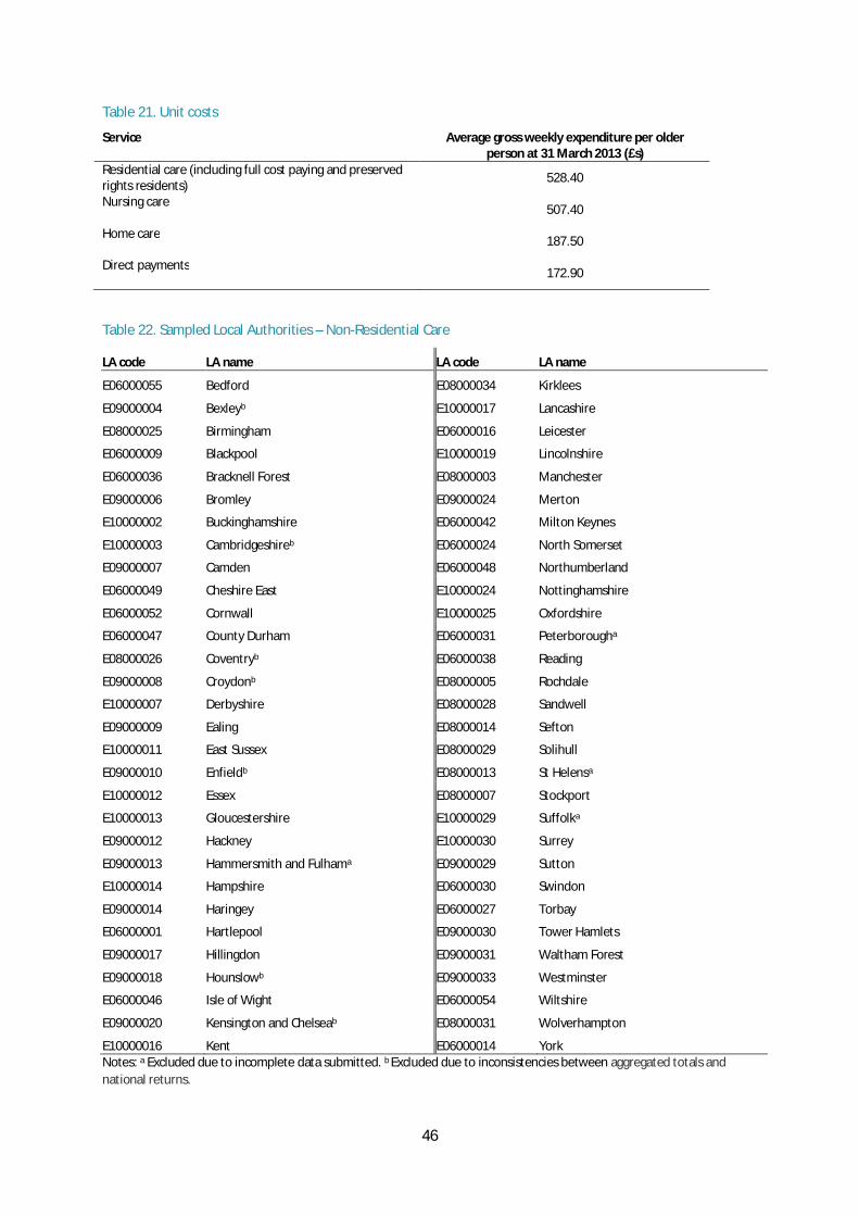
46

Table 21. Unit costs

Service Average gross weekly expenditure per older person at 31 March 2013 (£s)

Residential care (including full cost paying and preserved rights residents) 528.40

Nursing care 507.40

Home care 187.50

Direct payments 172.90

Table 22. Sampled Local Authorities – Non-Residential Care

LA code LA name LA code LA name

E06000055 Bedford E08000034 Kirklees

E09000004 Bexleyb E10000017 Lancashire

E08000025 Birmingham E06000016 Leicester

E06000009 Blackpool E10000019 Lincolnshire

E06000036 Bracknell Forest E08000003 Manchester

E09000006 Bromley E09000024 Merton

E10000002 Buckinghamshire E06000042 Milton Keynes

E10000003 Cambridgeshireb E06000024 North Somerset

E09000007 Camden E06000048 Northumberland

E06000049 Cheshire East E10000024 Nottinghamshire

E06000052 Cornwall E10000025 Oxfordshire

E06000047 County Durham E06000031 Peterborougha

E08000026 Coventryb E06000038 Reading

E09000008 Croydonb E08000005 Rochdale

E10000007 Derbyshire E08000028 Sandwell

E09000009 Ealing E08000014 Sefton

E10000011 East Sussex E08000029 Solihull

E09000010 Enfieldb E08000013 St Helensa

E10000012 Essex E08000007 Stockport

E10000013 Gloucestershire E10000029 Suffolka

E09000012 Hackney E10000030 Surrey

E09000013 Hammersmith and Fulhama E09000029 Sutton

E10000014 Hampshire E06000030 Swindon

E09000014 Haringey E06000027 Torbay

E06000001 Hartlepool E09000030 Tower Hamlets

E09000017 Hillingdon E09000031 Waltham Forest

E09000018 Hounslowb E09000033 Westminster

E06000046 Isle of Wight E06000054 Wiltshire

E09000020 Kensington and Chelseab E08000031 Wolverhampton

E10000016 Kent E06000014 York Notes: a Excluded due to incomplete data submitted. b Excluded due to inconsistencies between aggregated totals and national returns.

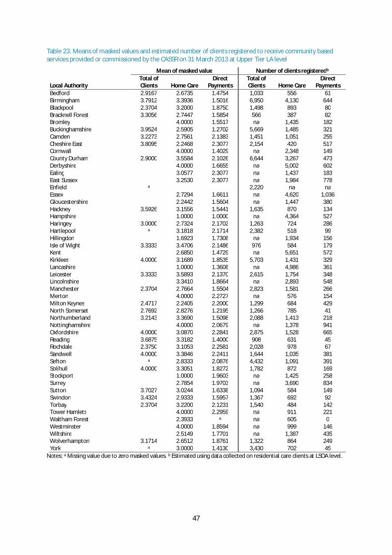
47

Table 23. Means of masked values and estimated number of clients registered to receive community based services provided or commissioned by the CASSR on 31 March 2013 at Upper Tier LA level

Mean of masked value Number of clients registeredb

Local Authority Total of Clients Home Care

Direct Payments

Total of Clients Home Care

Direct Payments

Bedford 2.9167 2.6735 1.4754 1,033 556 61 Birmingham 3.7912 3.3936 1.5016 6,950 4,130 644 Blackpool 2.3704 3.2000 1.8750 1,498 893 80 Bracknell Forest 3.3056 2.7447 1.5854 566 387 82 Bromley

4.0000 1.5517 na 1,435 182

Buckinghamshire 3.9524 2.5905 1.2702 5,669 1,485 321 Camden 3.2273 2.7561 2.1383 1,451 1,051 255 Cheshire East 3.8095 2.2468 2.3077 2,154 420 517 Cornwall

4.0000 1.4029 na 2,348 149

County Durham 2.9000 3.5584 2.1026 6,644 3,267 473 Derbyshire

4.0000 1.6655 na 5,002 602

Ealing

3.0577 2.3077 na 1,437 183 East Sussex

3.2530 2.3077 na 1,984 778

Enfield a

2,220 na na Essex

2.7294 1.6611 na 4,620 1,036

Gloucestershire

2.2442 1.5604 na 1,447 380 Hackney 3.5926 3.1556 1.5441 1,635 870 134 Hampshire

1.0000 1.0000 na 4,364 527

Haringey 3.0000 2.7324 2.1702 1,263 724 286 Hartlepool a 3.1818 2.1714 2,382 518 99 Hillingdon

1.6923 1.7308 na 1,934 156

Isle of Wight 3.3333 3.4706 2.1486 976 584 179 Kent

2.6850 1.4729 na 5,651 572

Kirklees 4.0000 3.1689 1.8535 5,703 1,431 329 Lancashire

1.0000 1.3608 na 4,986 361

Leicester 3.3333 3.5893 2.1370 2,615 1,754 348 Lincolnshire

3.3410 1.8664 na 2,893 548

Manchester 2.3704 2.7664 1.5504 2,823 1,581 266 Merton

4.0000 2.2727 na 576 154

Milton Keynes 2.4717 2.2405 2.2000 1,299 684 429 North Somerset 2.7692 2.8276 1.2195 1,266 785 41 Northumberland 3.2143 3.3690 1.5098 2,088 1,413 218 Nottinghamshire

4.0000 2.0679 na 1,378 941

Oxfordshire 4.0000 3.0870 2.2841 2,875 1,528 665 Reading 3.6875 3.3182 1.4000 908 631 45 Rochdale 2.3750 3.1053 2.2581 2,028 978 67 Sandwell 4.0000 3.3846 2.2411 1,644 1,035 381 Sefton a 2.8333 2.0876 4,432 1,091 391 Solihull 4.0000 3.3051 1.8272 1,782 872 169 Stockport

1.0000 1.9603 na 1,425 258

Surrey

2.7854 1.9703 na 3,690 834 Sutton 3.7027 3.0244 1.6338 1,094 584 149 Swindon 3.4324 2.9333 1.5957 1,367 692 92 Torbay 2.3704 3.2200 2.1231 1,540 484 142 Tower Hamlets

4.0000 2.2959 na 911 221

Waltham Forest

2.3933 a na 605 0

Westminster

4.0000 1.8594 na 999 146 Wiltshire

2.5149 1.7701 na 1,387 435

Wolverhampton 3.1714 2.6512 1.8761 1,322 864 249 York a 3.0000 1.4130 3,430 702 45

Notes: a Missing value due to zero masked values. b Estimated using data collected on residential care clients at LSOA level.

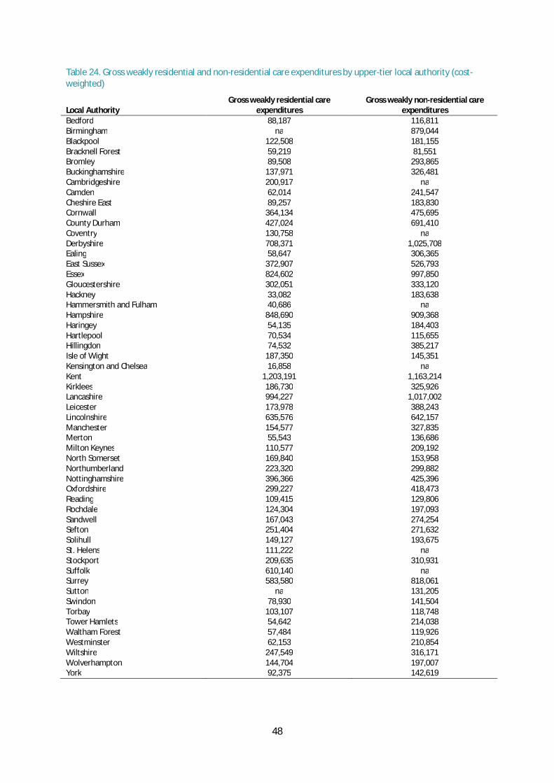
48

Table 24. Gross weakly residential and non-residential care expenditures by upper-tier local authority (cost-weighted)

Local Authority Gross weakly residential care

expenditures Gross weakly non-residential care

expenditures Bedford 88,187 116,811 Birmingham na 879,044 Blackpool 122,508 181,155 Bracknell Forest 59,219 81,551 Bromley 89,508 293,865 Buckinghamshire 137,971 326,481 Cambridgeshire 200,917 na Camden 62,014 241,547 Cheshire East 89,257 183,830 Cornwall 364,134 475,695 County Durham 427,024 691,410 Coventry 130,758 na Derbyshire 708,371 1,025,708 Ealing 58,647 306,365 East Sussex 372,907 526,793 Essex 824,602 997,850 Gloucestershire 302,051 333,120 Hackney 33,082 183,638 Hammersmith and Fulham 40,686 na Hampshire 848,690 909,368 Haringey 54,135 184,403 Hartlepool 70,534 115,655 Hillingdon 74,532 385,217 Isle of Wight 187,350 145,351 Kensington and Chelsea 16,858 na Kent 1,203,191 1,163,214 Kirklees 186,730 325,926 Lancashire 994,227 1,017,002 Leicester 173,978 388,243 Lincolnshire 635,576 642,157 Manchester 154,577 327,835 Merton 55,543 136,686 Milton Keynes 110,577 209,192 North Somerset 169,840 153,958 Northumberland 223,320 299,882 Nottinghamshire 396,366 425,396 Oxfordshire 299,227 418,473 Reading 109,415 129,806 Rochdale 124,304 197,093 Sandwell 167,043 274,254 Sefton 251,404 271,632 Solihull 149,127 193,675 St. Helens 111,222 na Stockport 209,635 310,931 Suffolk 610,140 na Surrey 583,580 818,061 Sutton na 131,205 Swindon 78,930 141,504 Torbay 103,107 118,748 Tower Hamlets 54,642 214,038 Waltham Forest 57,484 119,926 Westminster 62,153 210,854 Wiltshire 247,549 316,171 Wolverhampton 144,704 197,007 York 92,375 142,619

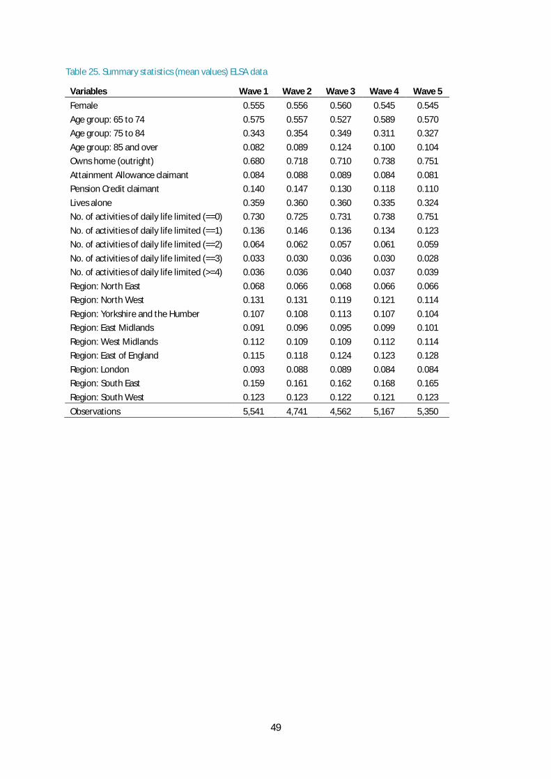
49

Table 25. Summary statistics (mean values) ELSA data

Variables Wave 1 Wave 2 Wave 3 Wave 4 Wave 5 Female 0.555 0.556 0.560 0.545 0.545 Age group: 65 to 74 0.575 0.557 0.527 0.589 0.570 Age group: 75 to 84 0.343 0.354 0.349 0.311 0.327 Age group: 85 and over 0.082 0.089 0.124 0.100 0.104 Owns home (outright) 0.680 0.718 0.710 0.738 0.751 Attainment Allowance claimant 0.084 0.088 0.089 0.084 0.081 Pension Credit claimant 0.140 0.147 0.130 0.118 0.110 Lives alone 0.359 0.360 0.360 0.335 0.324 No. of activities of daily life limited (==0) 0.730 0.725 0.731 0.738 0.751 No. of activities of daily life limited (==1) 0.136 0.146 0.136 0.134 0.123 No. of activities of daily life limited (==2) 0.064 0.062 0.057 0.061 0.059 No. of activities of daily life limited (==3) 0.033 0.030 0.036 0.030 0.028 No. of activities of daily life limited (>=4) 0.036 0.036 0.040 0.037 0.039 Region: North East 0.068 0.066 0.068 0.066 0.066 Region: North West 0.131 0.131 0.119 0.121 0.114 Region: Yorkshire and the Humber 0.107 0.108 0.113 0.107 0.104 Region: East Midlands 0.091 0.096 0.095 0.099 0.101 Region: West Midlands 0.112 0.109 0.109 0.112 0.114 Region: East of England 0.115 0.118 0.124 0.123 0.128 Region: London 0.093 0.088 0.089 0.084 0.084 Region: South East 0.159 0.161 0.162 0.168 0.165 Region: South West 0.123 0.123 0.122 0.121 0.123 Observations 5,541 4,741 4,562 5,167 5,350

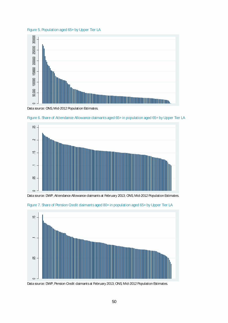
50

Figure 5. Population aged 65+ by Upper Tier LA

Data source: ONS, Mid-2012 Population Estimates. Figure 6. Share of Attendance Allowance claimants aged 65+ in population aged 65+ by Upper Tier LA

Data source: DWP, Attendance Allowance claimants at February 2013; ONS, Mid-2012 Population Estimates. Figure 7. Share of Pension Credit claimants aged 80+ in population aged 65+ by Upper Tier LA

Data source: DWP, Pension Credit claimants at February 2013; ONS, Mid-2012 Population Estimates.

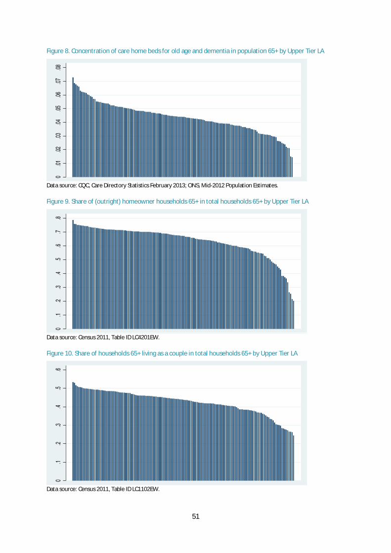
51

Figure 8. Concentration of care home beds for old age and dementia in population 65+ by Upper Tier LA

Data source: CQC, Care Directory Statistics February 2013; ONS, Mid-2012 Population Estimates. Figure 9. Share of (outright) homeowner households 65+ in total households 65+ by Upper Tier LA

Data source: Census 2011, Table ID LC4201EW. Figure 10. Share of households 65+ living as a couple in total households 65+ by Upper Tier LA

Data source: Census 2011, Table ID LC1102EW.

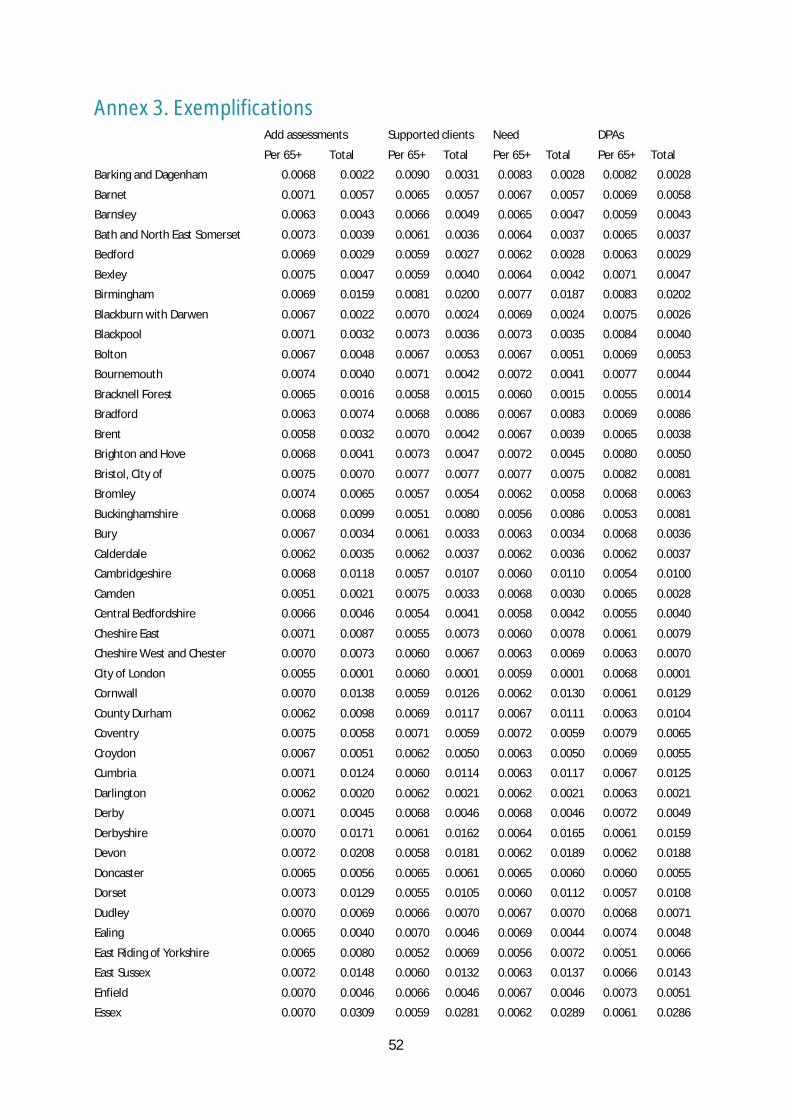
52

Annex 3. Exemplifications Add assessments Supported clients Need DPAs

Per 65+ Total Per 65+ Total Per 65+ Total Per 65+ Total

Barking and Dagenham 0.0068 0.0022 0.0090 0.0031 0.0083 0.0028 0.0082 0.0028

Barnet 0.0071 0.0057 0.0065 0.0057 0.0067 0.0057 0.0069 0.0058

Barnsley 0.0063 0.0043 0.0066 0.0049 0.0065 0.0047 0.0059 0.0043

Bath and North East Somerset 0.0073 0.0039 0.0061 0.0036 0.0064 0.0037 0.0065 0.0037

Bedford 0.0069 0.0029 0.0059 0.0027 0.0062 0.0028 0.0063 0.0029

Bexley 0.0075 0.0047 0.0059 0.0040 0.0064 0.0042 0.0071 0.0047

Birmingham 0.0069 0.0159 0.0081 0.0200 0.0077 0.0187 0.0083 0.0202

Blackburn with Darwen 0.0067 0.0022 0.0070 0.0024 0.0069 0.0024 0.0075 0.0026

Blackpool 0.0071 0.0032 0.0073 0.0036 0.0073 0.0035 0.0084 0.0040

Bolton 0.0067 0.0048 0.0067 0.0053 0.0067 0.0051 0.0069 0.0053

Bournemouth 0.0074 0.0040 0.0071 0.0042 0.0072 0.0041 0.0077 0.0044

Bracknell Forest 0.0065 0.0016 0.0058 0.0015 0.0060 0.0015 0.0055 0.0014

Bradford 0.0063 0.0074 0.0068 0.0086 0.0067 0.0083 0.0069 0.0086

Brent 0.0058 0.0032 0.0070 0.0042 0.0067 0.0039 0.0065 0.0038

Brighton and Hove 0.0068 0.0041 0.0073 0.0047 0.0072 0.0045 0.0080 0.0050

Bristol, City of 0.0075 0.0070 0.0077 0.0077 0.0077 0.0075 0.0082 0.0081

Bromley 0.0074 0.0065 0.0057 0.0054 0.0062 0.0058 0.0068 0.0063

Buckinghamshire 0.0068 0.0099 0.0051 0.0080 0.0056 0.0086 0.0053 0.0081

Bury 0.0067 0.0034 0.0061 0.0033 0.0063 0.0034 0.0068 0.0036

Calderdale 0.0062 0.0035 0.0062 0.0037 0.0062 0.0036 0.0062 0.0037

Cambridgeshire 0.0068 0.0118 0.0057 0.0107 0.0060 0.0110 0.0054 0.0100

Camden 0.0051 0.0021 0.0075 0.0033 0.0068 0.0030 0.0065 0.0028

Central Bedfordshire 0.0066 0.0046 0.0054 0.0041 0.0058 0.0042 0.0055 0.0040

Cheshire East 0.0071 0.0087 0.0055 0.0073 0.0060 0.0078 0.0061 0.0079

Cheshire West and Chester 0.0070 0.0073 0.0060 0.0067 0.0063 0.0069 0.0063 0.0070

City of London 0.0055 0.0001 0.0060 0.0001 0.0059 0.0001 0.0068 0.0001

Cornwall 0.0070 0.0138 0.0059 0.0126 0.0062 0.0130 0.0061 0.0129

County Durham 0.0062 0.0098 0.0069 0.0117 0.0067 0.0111 0.0063 0.0104

Coventry 0.0075 0.0058 0.0071 0.0059 0.0072 0.0059 0.0079 0.0065

Croydon 0.0067 0.0051 0.0062 0.0050 0.0063 0.0050 0.0069 0.0055

Cumbria 0.0071 0.0124 0.0060 0.0114 0.0063 0.0117 0.0067 0.0125

Darlington 0.0062 0.0020 0.0062 0.0021 0.0062 0.0021 0.0063 0.0021

Derby 0.0071 0.0045 0.0068 0.0046 0.0068 0.0046 0.0072 0.0049

Derbyshire 0.0070 0.0171 0.0061 0.0162 0.0064 0.0165 0.0061 0.0159

Devon 0.0072 0.0208 0.0058 0.0181 0.0062 0.0189 0.0062 0.0188

Doncaster 0.0065 0.0056 0.0065 0.0061 0.0065 0.0060 0.0060 0.0055

Dorset 0.0073 0.0129 0.0055 0.0105 0.0060 0.0112 0.0057 0.0108

Dudley 0.0070 0.0069 0.0066 0.0070 0.0067 0.0070 0.0068 0.0071

Ealing 0.0065 0.0040 0.0070 0.0046 0.0069 0.0044 0.0074 0.0048

East Riding of Yorkshire 0.0065 0.0080 0.0052 0.0069 0.0056 0.0072 0.0051 0.0066

East Sussex 0.0072 0.0148 0.0060 0.0132 0.0063 0.0137 0.0066 0.0143

Enfield 0.0070 0.0046 0.0066 0.0046 0.0067 0.0046 0.0073 0.0051

Essex 0.0070 0.0309 0.0059 0.0281 0.0062 0.0289 0.0061 0.0286

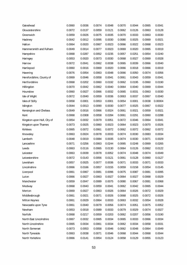
53

Gateshead 0.0060 0.0036 0.0074 0.0048 0.0070 0.0044 0.0065 0.0041

Gloucestershire 0.0072 0.0137 0.0059 0.0121 0.0062 0.0126 0.0063 0.0128

Greenwich 0.0059 0.0026 0.0075 0.0035 0.0070 0.0033 0.0063 0.0030

Hackney 0.0042 0.0012 0.0095 0.0030 0.0080 0.0025 0.0069 0.0021

Halton 0.0064 0.0020 0.0067 0.0023 0.0066 0.0022 0.0068 0.0023

Hammersmith and Fulham 0.0049 0.0014 0.0077 0.0023 0.0069 0.0020 0.0065 0.0019

Hampshire 0.0068 0.0287 0.0052 0.0235 0.0057 0.0251 0.0054 0.0240

Haringey 0.0053 0.0020 0.0073 0.0030 0.0068 0.0027 0.0069 0.0028

Harrow 0.0072 0.0041 0.0062 0.0038 0.0065 0.0039 0.0066 0.0040

Hartlepool 0.0060 0.0016 0.0069 0.0020 0.0066 0.0018 0.0066 0.0019

Havering 0.0076 0.0054 0.0063 0.0048 0.0066 0.0050 0.0074 0.0056

Herefordshire, County of 0.0069 0.0046 0.0058 0.0041 0.0061 0.0043 0.0059 0.0041

Hertfordshire 0.0068 0.0202 0.0060 0.0192 0.0062 0.0195 0.0060 0.0190

Hillingdon 0.0070 0.0042 0.0062 0.0040 0.0064 0.0040 0.0069 0.0044

Hounslow 0.0060 0.0027 0.0066 0.0032 0.0065 0.0031 0.0063 0.0030

Isle of Wight 0.0072 0.0040 0.0059 0.0036 0.0063 0.0037 0.0067 0.0040

Isles of Scilly 0.0058 0.0001 0.0053 0.0001 0.0054 0.0001 0.0038 0.00004

Islington 0.0044 0.0013 0.0090 0.0030 0.0077 0.0025 0.0067 0.0022

Kensington and Chelsea 0.0049 0.0016 0.0066 0.0024 0.0061 0.0021 0.0059 0.0021

Kent 0.0068 0.0308 0.0058 0.0284 0.0061 0.0291 0.0060 0.0288

Kingston upon Hull, City of 0.0054 0.0032 0.0079 0.0051 0.0072 0.0046 0.0064 0.0041

Kingston upon Thames 0.0073 0.0025 0.0060 0.0023 0.0064 0.0023 0.0070 0.0026

Kirklees 0.0065 0.0072 0.0061 0.0072 0.0062 0.0072 0.0062 0.0072

Knowsley 0.0063 0.0024 0.0078 0.0033 0.0074 0.0030 0.0083 0.0034

Lambeth 0.0048 0.0019 0.0084 0.0035 0.0074 0.0030 0.0071 0.0029

Lancashire 0.0071 0.0256 0.0063 0.0244 0.0065 0.0248 0.0069 0.0265

Leeds 0.0063 0.0116 0.0065 0.0130 0.0064 0.0126 0.0062 0.0122

Leicester 0.0063 0.0039 0.0078 0.0052 0.0074 0.0048 0.0074 0.0049

Leicestershire 0.0072 0.0143 0.0056 0.0121 0.0061 0.0128 0.0060 0.0127

Lewisham 0.0057 0.0025 0.0077 0.0036 0.0071 0.0033 0.0071 0.0033

Lincolnshire 0.0066 0.0166 0.0057 0.0155 0.0059 0.0158 0.0054 0.0145

Liverpool 0.0061 0.0067 0.0081 0.0096 0.0075 0.0087 0.0081 0.0095

Luton 0.0066 0.0027 0.0063 0.0027 0.0064 0.0027 0.0068 0.0029

Manchester 0.0059 0.0047 0.0089 0.0075 0.0080 0.0067 0.0081 0.0068

Medway 0.0068 0.0043 0.0059 0.0041 0.0062 0.0042 0.0065 0.0044

Merton 0.0069 0.0027 0.0063 0.0026 0.0064 0.0026 0.0072 0.0029

Middlesbrough 0.0061 0.0021 0.0071 0.0026 0.0068 0.0025 0.0072 0.0026

Milton Keynes 0.0061 0.0029 0.0064 0.0033 0.0063 0.0032 0.0054 0.0028

Newcastle upon Tyne 0.0061 0.0040 0.0079 0.0056 0.0074 0.0051 0.0075 0.0052

Newham 0.0053 0.0018 0.0089 0.0033 0.0079 0.0029 0.0074 0.0027

Norfolk 0.0068 0.0217 0.0059 0.0203 0.0062 0.0207 0.0056 0.0190

North East Lincolnshire 0.0067 0.0032 0.0065 0.0034 0.0065 0.0033 0.0066 0.0034

North Lincolnshire 0.0065 0.0034 0.0061 0.0034 0.0062 0.0034 0.0058 0.0031

North Somerset 0.0073 0.0053 0.0058 0.0046 0.0062 0.0048 0.0064 0.0049

North Tyneside 0.0063 0.0038 0.0071 0.0046 0.0068 0.0044 0.0068 0.0044

North Yorkshire 0.0066 0.0141 0.0054 0.0124 0.0058 0.0129 0.0055 0.0123

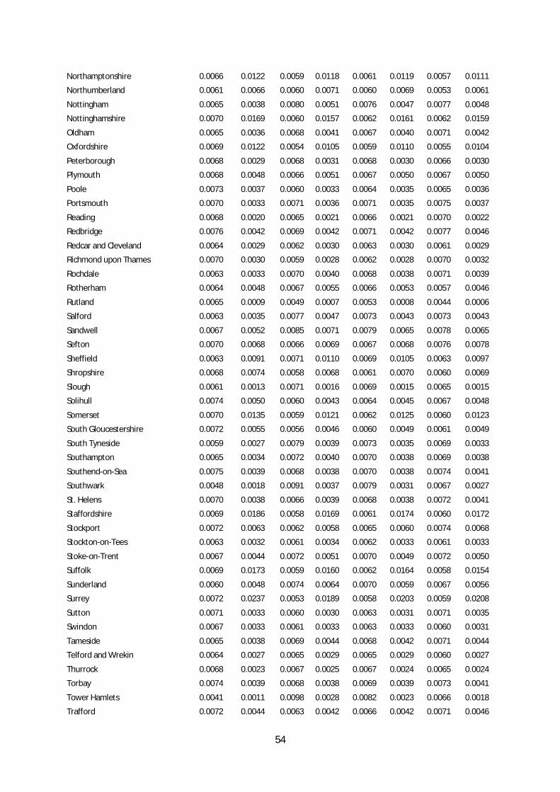
54

Northamptonshire 0.0066 0.0122 0.0059 0.0118 0.0061 0.0119 0.0057 0.0111

Northumberland 0.0061 0.0066 0.0060 0.0071 0.0060 0.0069 0.0053 0.0061

Nottingham 0.0065 0.0038 0.0080 0.0051 0.0076 0.0047 0.0077 0.0048

Nottinghamshire 0.0070 0.0169 0.0060 0.0157 0.0062 0.0161 0.0062 0.0159

Oldham 0.0065 0.0036 0.0068 0.0041 0.0067 0.0040 0.0071 0.0042

Oxfordshire 0.0069 0.0122 0.0054 0.0105 0.0059 0.0110 0.0055 0.0104

Peterborough 0.0068 0.0029 0.0068 0.0031 0.0068 0.0030 0.0066 0.0030

Plymouth 0.0068 0.0048 0.0066 0.0051 0.0067 0.0050 0.0067 0.0050

Poole 0.0073 0.0037 0.0060 0.0033 0.0064 0.0035 0.0065 0.0036

Portsmouth 0.0070 0.0033 0.0071 0.0036 0.0071 0.0035 0.0075 0.0037

Reading 0.0068 0.0020 0.0065 0.0021 0.0066 0.0021 0.0070 0.0022

Redbridge 0.0076 0.0042 0.0069 0.0042 0.0071 0.0042 0.0077 0.0046

Redcar and Cleveland 0.0064 0.0029 0.0062 0.0030 0.0063 0.0030 0.0061 0.0029

Richmond upon Thames 0.0070 0.0030 0.0059 0.0028 0.0062 0.0028 0.0070 0.0032

Rochdale 0.0063 0.0033 0.0070 0.0040 0.0068 0.0038 0.0071 0.0039

Rotherham 0.0064 0.0048 0.0067 0.0055 0.0066 0.0053 0.0057 0.0046

Rutland 0.0065 0.0009 0.0049 0.0007 0.0053 0.0008 0.0044 0.0006

Salford 0.0063 0.0035 0.0077 0.0047 0.0073 0.0043 0.0073 0.0043

Sandwell 0.0067 0.0052 0.0085 0.0071 0.0079 0.0065 0.0078 0.0065

Sefton 0.0070 0.0068 0.0066 0.0069 0.0067 0.0068 0.0076 0.0078

Sheffield 0.0063 0.0091 0.0071 0.0110 0.0069 0.0105 0.0063 0.0097

Shropshire 0.0068 0.0074 0.0058 0.0068 0.0061 0.0070 0.0060 0.0069

Slough 0.0061 0.0013 0.0071 0.0016 0.0069 0.0015 0.0065 0.0015

Solihull 0.0074 0.0050 0.0060 0.0043 0.0064 0.0045 0.0067 0.0048

Somerset 0.0070 0.0135 0.0059 0.0121 0.0062 0.0125 0.0060 0.0123

South Gloucestershire 0.0072 0.0055 0.0056 0.0046 0.0060 0.0049 0.0061 0.0049

South Tyneside 0.0059 0.0027 0.0079 0.0039 0.0073 0.0035 0.0069 0.0033

Southampton 0.0065 0.0034 0.0072 0.0040 0.0070 0.0038 0.0069 0.0038

Southend-on-Sea 0.0075 0.0039 0.0068 0.0038 0.0070 0.0038 0.0074 0.0041

Southwark 0.0048 0.0018 0.0091 0.0037 0.0079 0.0031 0.0067 0.0027

St. Helens 0.0070 0.0038 0.0066 0.0039 0.0068 0.0038 0.0072 0.0041

Staffordshire 0.0069 0.0186 0.0058 0.0169 0.0061 0.0174 0.0060 0.0172

Stockport 0.0072 0.0063 0.0062 0.0058 0.0065 0.0060 0.0074 0.0068

Stockton-on-Tees 0.0063 0.0032 0.0061 0.0034 0.0062 0.0033 0.0061 0.0033

Stoke-on-Trent 0.0067 0.0044 0.0072 0.0051 0.0070 0.0049 0.0072 0.0050

Suffolk 0.0069 0.0173 0.0059 0.0160 0.0062 0.0164 0.0058 0.0154

Sunderland 0.0060 0.0048 0.0074 0.0064 0.0070 0.0059 0.0067 0.0056

Surrey 0.0072 0.0237 0.0053 0.0189 0.0058 0.0203 0.0059 0.0208

Sutton 0.0071 0.0033 0.0060 0.0030 0.0063 0.0031 0.0071 0.0035

Swindon 0.0067 0.0033 0.0061 0.0033 0.0063 0.0033 0.0060 0.0031

Tameside 0.0065 0.0038 0.0069 0.0044 0.0068 0.0042 0.0071 0.0044

Telford and Wrekin 0.0064 0.0027 0.0065 0.0029 0.0065 0.0029 0.0060 0.0027

Thurrock 0.0068 0.0023 0.0067 0.0025 0.0067 0.0024 0.0065 0.0024

Torbay 0.0074 0.0039 0.0068 0.0038 0.0069 0.0039 0.0073 0.0041

Tower Hamlets 0.0041 0.0011 0.0098 0.0028 0.0082 0.0023 0.0066 0.0018

Trafford 0.0072 0.0044 0.0063 0.0042 0.0066 0.0042 0.0071 0.0046

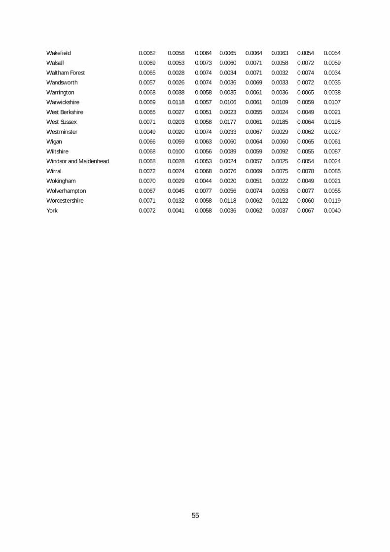
55

Wakefield 0.0062 0.0058 0.0064 0.0065 0.0064 0.0063 0.0054 0.0054

Walsall 0.0069 0.0053 0.0073 0.0060 0.0071 0.0058 0.0072 0.0059

Waltham Forest 0.0065 0.0028 0.0074 0.0034 0.0071 0.0032 0.0074 0.0034

Wandsworth 0.0057 0.0026 0.0074 0.0036 0.0069 0.0033 0.0072 0.0035

Warrington 0.0068 0.0038 0.0058 0.0035 0.0061 0.0036 0.0065 0.0038

Warwickshire 0.0069 0.0118 0.0057 0.0106 0.0061 0.0109 0.0059 0.0107

West Berkshire 0.0065 0.0027 0.0051 0.0023 0.0055 0.0024 0.0049 0.0021

West Sussex 0.0071 0.0203 0.0058 0.0177 0.0061 0.0185 0.0064 0.0195

Westminster 0.0049 0.0020 0.0074 0.0033 0.0067 0.0029 0.0062 0.0027

Wigan 0.0066 0.0059 0.0063 0.0060 0.0064 0.0060 0.0065 0.0061

Wiltshire 0.0068 0.0100 0.0056 0.0089 0.0059 0.0092 0.0055 0.0087

Windsor and Maidenhead 0.0068 0.0028 0.0053 0.0024 0.0057 0.0025 0.0054 0.0024

Wirral 0.0072 0.0074 0.0068 0.0076 0.0069 0.0075 0.0078 0.0085

Wokingham 0.0070 0.0029 0.0044 0.0020 0.0051 0.0022 0.0049 0.0021

Wolverhampton 0.0067 0.0045 0.0077 0.0056 0.0074 0.0053 0.0077 0.0055

Worcestershire 0.0071 0.0132 0.0058 0.0118 0.0062 0.0122 0.0060 0.0119

York 0.0072 0.0041 0.0058 0.0036 0.0062 0.0037 0.0067 0.0040

56

References Bebbington, A. and B. Davies (1980). "Territorial need indicators: a new approach." Journal of Social

Policy 9(2): 145–68. Cmnd 6453 (1976). Local Government Finance. Report of the Committee of Enquiry (Chairman: F.

Layfield, Esq., QC). London, HMSO Darton, R., J. Forder, A. Netten, A. Bebbington, J. Holder and A. M. Towers (2010). "Slicing Up the Pie:

Allocation of Central Government Funding of Care of Older People." Social Policy & Administration 44(5): 529-553.

Department of Health (2010). Prioritising need in the context of Putting People First: A whole system approach to eligibility for social care. London

Department of Health (2013) Caring for our future: Consultation on reforming what and how people pay for their care and support, DH (gov.uk) (https://www.gov.uk/government/uploads/system/uploads/attachment_data/file/239393/CONSULTATION_CaringForOurFuture_acc.pdf)

Department of Health (2013). Draft national minimum eligibility threshold for adult care and support: A discussion document. London

Fernandez, J.-L. and T. Snell (2014). Exploring the use of micro data for estimating a Relative Needs Formula for older people’s additional assessments following the introduction of a universal cap on social care expenditure PSSRU Discussion Paper 2875. London, PSSRU, London School of Economics

Fernandez, J., J. Forder and M. Knapp (2011). Long-term care. The Oxford Handbook of Health Economics. P. Smith and S. Glied. Oxford, Oxford University Press.

Fernandez, J. and T. Snell (2012). Survey of Fair Access to Care Services (FACS) asses sment criteria among local authorities in England PSSRU Discussion Paper 2012, PSSRU, London School of Economics (https://www.lse.ac.uk/LSEHealthAndSocialCare/pdf/FACS-eligibility-report-dp-2825f.pdf)

Fernandez, J. L. and J. Forder (2010). "Equity, efficiency, and financial risk of alternative arrangements for funding long-term care systems in an ageing society." Oxford Review of Economic Policy 26(4): 713-733.

Forder, J. and J. L. Fernández (2009). Analysing the costs and benefits of social care funding arrangements in England: technical report (1st Edition). PSSRU DP 2644, PSSRU, University of Kent and London School of Economics (http://www.pssru.ac.uk/pdf/dp2644.pdf)

Gravelle, H., M. Sutton, S. Morris, F. Windmeijer, A. Leyland, C. Dibben and M. Muirhead (2003). "Modelling supply and demand infuences on the use of health care: implications for deriving a needs-based capitation formula." Health Economics 12: 985–1004.

Smith, P. (2007). Formula Funding of Public Services. London and New York, Routledge. Wanless, D., J. Forder, J.-L. Fernandez, T. Poole, L. Beesley, M. Henwood and F. Moscone (2006).

Securing Good Care for Older People: Taking a long term view. London, King's Fund

Documents

Estimating relative needs formulae for new forms of …eprints.lse.ac.uk/59073/1/__lse.ac.uk_storage_LIBRARY_Secondary... · The number of people satisfying eligibility tests for