Alex Haberis and Andrej Sokol

A procedure for combining zero and sign restrictions in a VAR-identification scheme Discussion paper

Original citation: Haberis, Alex and Sokol, Andrej (2014) A procedure for combining zero and sign restrictions in a VAR-identification scheme. CFM discussion paper series, CFM-DP2014-10. Centre For Macroeconomics, London, UK.

Originally available from the Centre For Macroeconomics This version available at: http://eprints.lse.ac.uk/58077/ Available in LSE Research Online: July 2014 © 2014 The Authors LSE has developed LSE Research Online so that users may access research output of the School. Copyright © and Moral Rights for the papers on this site are retained by the individual authors and/or other copyright owners. Users may download and/or print one copy of any article(s) in LSE Research Online to facilitate their private study or for non-commercial research. You may not engage in further distribution of the material or use it for any profit-making activities or any commercial gain. You may freely distribute the URL (http://eprints.lse.ac.uk) of the LSE Research Online website.

A Procedure for Combining Zero and Sign Restrictions in a

VAR-Identification Scheme ∗

Alex Haberis†and Andrej Sokol‡

5 June 2014

Abstract

In this paper we describe a procedure for implementing zero restrictions within the context of a sign

restrictions identification scheme for VARs. The procedure introduces an additional step into the algorithm

outlined in Fry and Pagan (2011) and Rubio-Ramirez et al. (2006) for implementing sign restrictions. This

extra step involves rotating a candidate identification matrix using Givens rotation matrices to introduce

zero restrictions. We then check whether the elements of the candidate matrix satisfy the sign restrictions

as usual. We illustrate how our procedure works by generating artificial data from the theoretical model of

An and Schorfheide (2007), which implies certain restrictions on the impact of its structural shocks on the

model’s endogenous variables. We exploit our knowledge of that pattern to identify structural shocks from

the reduced-form errors of a VAR estimated on the simulated data.

JEL: C32, C51, E12

∗We would like to thank Luca Benati, Richard Harrison, Francesca Monti, Roland Meeks, Haroon Mumtaz, Matthias Paustian,

Konstantinos Theodoridis, and Tony Yates for useful discussions. The views expressed in this paper are solely the responsibility of

the authors and should not be interpreted as reflecting the views of the Bank of England.†Bank of England and Centre for Macroeconomics. Email: alex.haberis@bankofengland.co.uk‡Bank of England. Email: andrej.sokol@bankofengland.co.uk

1

1 Introduction

A central aim of structural vector-autoregression analysis is to uncover economically-interpretable – ‘structural’

– shocks that drive dynamics of macroeconomic variables in the data. Economic theory is widely used to

motivate the restrictions that are necessary to identify structural shocks from the reduced-form innovations to

a vector autoregression (VAR). In recent years, a growing literature has used sign restrictions on the impulse

response functions (IRFs) of a VAR to identify economic shocks in the data. The source of these restrictions

can be a formal model. For example, the IRFs of a dynamic stochastic general equilibrium (DSGE) model will

imply a pattern of co-movement among the model’s endogenous variables that can be used to inform the sign

restrictions on the IRFs of a VAR. Alternatively, the restrictions might be based on a view of the effects of a

shock on certain variables that is not derived from a fully-specified model1.

In either case, as well as having implications about the signs of the responses, economic theory can imply

that certain variables do not respond at all to some shocks. This suggests that, in addition to sign restrictions,

zero restrictions can be used to identify the effects of economic shocks in the data. Indeed, it may be the case

that zero restrictions are essential to identify the effects of some shocks. An example of a shock that induces

a zero response among economic variables can be found in the New Keynesian literature, where monetary

policy can be specified to entirely offset the impact of demand shocks on inflation. Another policy example is

the assessment of the size of the ‘balanced-budget’ fiscal multiplier, i.e. the impact on output from a policy

that involves exogenously changing government spending and taxes in a way that leaves the primary balance

unchanged. The impulse response of the primary balance to such a shock would be zero on impact.2

In this paper, we outline a procedure for implementing zero restrictions in the context of a sign restrictions

identification scheme. This extends the methodology outlined in Baumeister and Benati (2013) to allow for

multiple zero restrictions. In related work, Arias et al. (2014) also propose an algorithm to implement zero

restrictions on the IRFs of a VAR. The difference between their procedure and ours is that we use a combi-

nation of Givens and Householder transformations to generate candidate structures that satisify the zero and

sign restrictions, whereas Arias et al. (2014) use only Householder transformations, although with additional

orthogonality restrictions, to deliver the zero restrictions. In this paper we do not attempt a comparison of the

relative performance of the two algorithms, which we leave for future research.

We illustrate our procedure by applying it to the simple New Keynesian model described in An and

Schorfheide (2007). The rational expectations equilibrium of this model has a first-order VAR representa-

tion so it is, in principle, possible to obtain empirical estimates of the model’s IRFs using a VAR estimated on

data for the model’s observable variables. However, the model’s specification of monetary policy implies infla-

tion does not respond at all to government spending shocks. As a result, there are zero responses in the model’s

IRFs, and it would not be possible to identify the government spending shock using only sign restrictions – zero

1Fry and Pagan (2011) review papers in the sign restrictions literature and distinguish between studies in which the sign

restrictions come from a formal model or otherwise.2Though not necessarily thereafter, depending on the implementation of the policy.

2

restrictions are essential to identify this shock. So we simulate data from the model, estimate a VAR on the

simulated data for the observable variables, and identify the structural shocks using a combination of sign and

zero restrictions implied by the DSGE model. We show that our procedure does well in recovering the correct

impulse responses from the original model.

The paper is organised as follows. In Section 2, we illustrate why VAR impulse responses may include zero

responses; in Section 3, we outline our algorithm for introducing zero restrictions using an application to the

An and Schorfheide (2007) model; in Section 4 we conclude.

2 When zero restrictions on VAR impulse response functions are

required

To illustrate how economic theory can provide the motivation for zero restrictions in a VAR-identification

scheme, we focus on a special case in which the shocks in an economic model match up with the shocks

associated with a VAR. This will only be true when the model has a finite-order VAR representation. In this

case, a structural VAR will give accurate estimates of the IRFs to the economic shocks that are of interest.

Our approach for introducing zeros, however, is not restricted to this case. It is possible that the sign and zero

restrictions used to identify the VAR are not derived from a well-defined model; Fry and Pagan (2011) discuss

papers that use this approach. That said, since in Section 3 we illustrate our procedure using data artificially

generated from a model, it is convenient to consider an economic model with a finite-order VAR representation.

This allows us to side-step two issues in VAR analysis which, although of practical and theoretical significance,

are not the focus of this paper. First, if a model does not have a well-defined VAR representation, a VAR

estimated on data for the model’s observable variables may be relatively uninformative about economic shocks

one wishes to identify, as discussed by Fernandez-Villaverde et al. (2007). Second, considering a model whose

VAR representation is of finite order allows us to avoid issues related to the potential ‘truncation bias’ introduced

by estimating a finite-order VAR when the ‘true’ model has a VAR representation of infinite order, as discussed

by Ravenna (2007).

2.1 VAR model

The issue of identifying shocks in a VAR can be outlined, without loss of generality, by considering a first-order

VAR model:

yt = βyt−1 + et (1)

where (yt is an ny×1) vector of observable variables and et is an (ny×1) vector of Normally-distributed errors,

for which E(et) = 0, E(ete′t) = Σ, and E(ete

′t−s) = 0 for s 6= 0.

To extract a vector of economically-interpretable shocks from the VAR errors, we need an identification

scheme. This can be represented by the matrix F, which transforms the VAR errors into an (ny × 1) vector of

3

orthogonal ‘structural’ shocks, εt, such that εt = F−1et. The structural shocks are Normally distibuted, with

E(εt) = 0, E(εtε′t) = I, and E(εtε

′t−s) = 0 for s 6= 0. Furthermore, the matrix F is constructed so that the

structural shocks are uncorrelated with each other, E(εi,tεj,t) = 0, and are consistent with a theory about the

effects of the economic shocks being estimated. Having contructed a matrix F, the emprical model can take the

form of a structural VAR:

yt = βyt−1 + Fεt (2)

2.2 Theoretical model

The equilibrium of a theoretical model can take the following state-space representation for yt:3

xt = Axt−1 + Bwt (3)

yt = Cxt−1 + Dwt (4)

where yt continues to denote an (ny × 1) vector of observable variables and xt is an (nx× 1) vector of (possibly

unobserved) state variables. The vector wt (ny × 1) includes both measurement errors and innovations to the

economically-interpretable structural shocks (e.g. shocks to technology, preferences, policy, and so on).4 They

are Normally distributed, with E(wt) = 0, E(wtw′t) = I, and E(wtw

′t−s) = 0 for s 6= 0. The coefficient

matrices A (nx × nx), B (nx × nw), C (ny × nx), and D (ny × ny) are functions of the deep parameters of the

model: technology, preferences, the persistence of the structural shocks, etc..

Provided certain conditions hold,5 economic models of the ABCD form – equations (3) and (4) – have a

finite-order VAR representation. This maps innovations to the structural shocks to the observable variables and

their lags. In a particular case, which is convenient for our exposition, the VAR representation of the economic

model will be first-order:6

yt = CAC−1yt−1 + Dwt. (5)

2.3 Theory-based identification of the VAR shocks

From equations (2) and (5) it is a clear that there is a correspondence between the economic model and the

SVAR. Therefore, to identify the SVAR shocks – i.e. to construct the matrix F – it is possible to draw on

the information in D about the pattern of responses – including zero responses – of the model’s endogenous

variables to the economic shocks, wt. For instance, restricting F to match the pattern of signs and zeros in D

would allow the structural shocks in the VAR, εt, to be interpreted as the economc shocks in the model, wt.

3This representation is based on Fernandez-Villaverde et al (2007).4Here we are considering the square case in which the number of shocks is equal to the number of observable variables.5As outlined by Fernandez-Villaverde et al. (2007) and Ravenna (2007).6This holds when B = AC−1D. See Morris (2013) for further details on the conditions under which a DSGE model has a

VAR(1) representation.

4

3 An algorithm for imposing zero and sign restrictions: illustrative

example

In this section we outline, using a simple application based on the model of An and Schorfheide (2007), our

algorithm for implementing zero and sign restrictions in a VAR-identification scheme.7 The aim of the algorithm

is to find a set of matrices that satisfy the sign and zero restrictions implied by D in the model’s VAR repre-

sentation, which we will denote by Fm, for m = 1, 2, ..., nM . Each matrix Fm represents an identified structure

rather than an identified model. The number of identified structures, nM , is chosen by the econometrician.8

Generalising Baumeister and Benati (2013), our approach combines the procedure for imposing sign restrictions

of Rubio-Ramirez et al. (2006) with the imposition of nz ≤ ny(ny−1)2 zero restrictions using an equal number of

Givens rotations matrices.9 The algorithm involves repeating a few steps many times until the required number

of matches, nM , are found.

Although our procedure is applicable to VAR-shock identification based on zero and sign restrictions in gen-

eral, the An and Schorfheide (2007) model is useful for expositional purposes insofar as its rational expectations

equilibrium has a VAR(1) representation which implies zero as well as sign restrictions. We can, therefore, gen-

erate artificial data from the model, estimate a VAR(1) on the simulated data, and then identify the structural

shocks using a combination of zero and sign restrictions. Before turning to the algorithm, we briefly describe

the model.

3.1 An and Schorfheide (2007) model

3.1.1 Theoretical model

The log-linearised equilibirum conditions and exogenous processes of the An and Schorfheide (2007) model take

the following form:

yt = Etyt+1 −1

τ(rt − Etπt+1 − Etzt+1) + gt − Etgt+1 (6)

πt = βEtπt+1 + κ (yt − gt) (7)

ct = yt − gt (8)

rt = ρr rt−1 + (1− ρr) (ψ1πt + ψ2 (yt − gt)) + εr,t (9)

gt = ρg gt−1 + εg,t (10)

zt = ρz zt−1 + εz,t (11)

7The general algorithm is described in Appendix A.8Fry and Pagan (2011) discuss the problem of structure versus model identification.9This maximum number of zero restrictions corresponds to the number of zeros in a triangular matrix. Indeed, the algorithm

described in this section can be used to triangularise a square matrix of size ny .

5

where yt is output, πt is inflation, ct is consumption, rt is the nominal interest rate, gt is government spending,

zt is technology, εr,t is a monetary policy shock, εg,t is a government spending shock, and εz,t is a technology

shock. The shocks are normally distributed with means zero and standard deviations σr, σg, and σz respectively.

The structure of the model is standard in the New Keynesian literature: equation (6) is the dynamic IS curve;

equation (7) is the New Keynesian Phillips curve; equation (8) is the aggregate goods market equilibrium;

equation (9) is the monetary policy rule; equations (10) and (11) are the exogenous processes for government

spending and technology.10

We adopt the same parameterisation as in An and Schorfheide (2007). The value of the intertemporal

elasticity of substitution, τ , is set to 2; the discount factor, β, is 0.9975; the elasticity of demand for intermediate

goods, ν−1, is 10; the degree of price stickiness, φ, is 53.6797; the steady state inflation rate, π, is 1.008; the

weight on inflation in policy rule, ψ1, is 1.5; the weight on consumption in policy rule, ψ2, is 0.125 ; the

persistence of government spending shock process, ρg, is 0.95; the persistence of technology shock process, ρz,

is 0.9; and the Phillips curve slope, κ ≡ τ(1−ν)νπ2φ , is 0.33.

The VAR(1) representation of the model’s rational expectations equilibrium is given by a system in which

the vector of observable variables is yt ≡ [ rt yt πt ]′, and the vector of shocks is wt ≡ [ εz,t εg,t εr,t ]′:11

rt

yt

πt

=

0.7902 0 0.2535

0.1944 0.95 −0.4642

0.1195 0 0.6242

rt−1

yt−1

πt−1

+

0.6055 0 0.6858

1.4863 1 −1.1011

1.4909 0 −0.7462

εz,t

εg,t

εr,t

(12)

From the D matrix in equation (12), it is clear that the model’s assumptions imply a set of contemporaneous

responses of the observable variables to the shocks that includes zeros. In particular, neither the nominal interest

rate nor inflation respond to the government spending shock. This is because, in the model, consumption – and

hence inflation via the Phillips curve, and nominal rates via the policy rule – are left unchanged by government

spending shocks. This reflects the model’s unit government-spending multiplier on output.

3.1.2 VAR estimation and identification scheme

To illustrate our procedure, we estimate a structural VAR(1) for the model’s observable variables on data

simulated from the theoretical model, equation (12).12 To identify the economic shocks from the reduced-form

VAR errors we use sign and zero restrictions consistent with the D matrix in equation (12), which are summarised

in Table 1. Clearly, only imposing the sign restriction that the government spending shock increases output

would be insufficient to identify this shock. And imposing additional sign restrictions would be inconsistent

with the theory. Therefore, the zero restrictions are essential to identify the government spending shock in this

model.

10The formulation of the Phillips curve and policy rule are slightly different to common specifications for these equations;

nevertheless, it is equivalent since, yt− gt, which is equal to consumption, is proportional to real marginal cost and the output gap.11See Morris (2012). See also Komunjer and Ng (2011) for further details on the model’s ABCD representation.12The parameter estimates for the VAR estimation are the same as the true data generating process in equation (12) to 4 decimal

places.

6

Technology shock Government spending shock Monetary policy shock

Nominal interest rate + 0 +

Output + + −

Inflation + 0 −Table 1: Sign and zero restrictions for identification scheme

3.2 Implementing the algorithm for zero and sign restrictions

The algorithm for imposing zero and sign restrictions involves iterating through four steps until the desired

number of candidate structures, nm, is found. Before starting starting the iterative stage of the algorithm, it is

necessary to take the Cholesky decomposition, F, of the estimated covariance matrix of the VAR errors, Σ:

F−1ΣF′−1 = Iny .

This defines a set of shocks εt ≡ F−1et that are uncorrelated and have unit variance, but do not necessarily

satisfy the sign and zero restrictions, where et are the estimated VAR errors.

In the iterative part of the algorithm, at each stage of the iteration, we generate orthonormal matrices

QG (i.e. QGQ′G = Iny) such that the uncorrelated, unit-variance shocks, εt ≡ (FQG)−1et ≡ F−1et satisfy

the sign and zero restrictions in Table 1, and have the same covariance matrix as the reduced-form errors,

E(FQG εtε′tQ′GF′) = FF′ = Σ. In particular, we repeat the following steps until nM matches have been found:

1. We take the QR decomposition of a random (ny × ny) Normal matrix, W:

W = QR

where Q is an orthogonal matrix (i.e. QQ′ = Q′Q = Iny ), and R is a triangular matrix. We now have a matrix

FQ and some uncorrelated, unit-variance shocks, εt:

et = FQεt

=

f11 f12 f13

f21 f22 f23

f31 f32 f33

ε1,t

ε2,t

ε3,t

2. We rotate FQ to introduce the zero restrictions, f12 = f32 = 0, by post-multiplying with two Givens

rotations matrices:

FQG1 (θ∗1) G2 (θ∗2) ≡ FQG ≡ F

where the Givens rotations are functions of the angles θ∗1 and θ∗2 . These two angles can be found by solving the

system of two simultaneous equations obtained by setting the (1, 2) and (3, 2) elements of F to zero. Writing

this out for clarity, starting with the first restriction, we can choose the following Givens matrix to set the

element in (1, 2) to zero:

G1 (θ1) =

cos θ1 − sin θ1 0

sin θ1 cos θ1 0

0 0 1

7

For the second zero restriction in (3, 2) we use the following Givens rotation:

G2 (θ2) =

1 0 0

0 cos θ2 − sin θ2

0 sin θ2 cos θ2

We then compute the product:

FQG1 (θ1) G2 (θ2) =

f11 f12 f13

f21 f22 f23

f31 f32 f33

cos θ1 − sin θ1 0

sin θ1 cos θ1 0

0 0 1

1 0 0

0 cos θ2 − sin θ2

0 sin θ2 cos θ2

Setting the expressions in the elements in (1, 2) and (3, 2) of this product gives the following pair of simul-

taneous equations, which can be solved for θ∗1 and θ∗2 :

f13 sin θ2 + cos θ2(f12 cos θ1 − f11 sin θ1) = 0

f33 sin θ2 + cos(f32 cos θ1 − f31 sin θ1) = 0

Having solved for the angles θ∗1 and θ∗2 , and used them to construct the Givens rotations, G1 (θ∗1) and

G2 (θ∗2), we have an orthonormal matrix, F, that satisfies the zero restrictions.

3. In this step, we check whether the non-zero elements in F match the sign restrictions in Table 1, and

retain the matrix if it does.

4. We go back to step 1 and repeat until nM matches have been found.

In our application we set nM to 500. As a result, we have 500 identified structures given by:

Fmεt = et.

for m = 1, 2, ..., 100, where εt can be interpreted as the shocks in the economic model.

3.2.1 Identified shocks

Figure 1 shows the estimated IRFs to the shocks for the 500 identified structures. In the figure, the swathes

of blue (plain) lines are the IRFs for each identified structure. The red (circled) lines are the “median target”

IRF calculated following Fry and Pagan (2011), i.e. the IRF – generated by one of our m structures – with

the smallest average distance from the median responses across the technology, government spending, and

monetary policy shocks. Finally, the green (crossed) lines are the IRFs from the model itself. The figure shows

the Fry-Pagan medians of the estimated IRFs match well the IRFs from the theoretical model, including the

zero responses for the government spending shock on inflation and the nominal interest rate.

3.3 Discussion

As noted above, Arias et al. (2014) also propose a procedure for implementing sign and zero restrictions, as

well as surveying earlier contributions. The difference between the algorithm proposed by Arias et al. (2014)

8

0 10 200

0.5

1rt response to ǫz,t

p.p.dev.from

s.s.

0 10 20−1

0

1rt response to ǫg,t

p.p.dev.from

s.s.

0 10 20−1

0

1rt response to ǫr,t

p.p.dev.from

s.s.

0 10 200

1

2yt response to ǫz ,t

percentdev.from

s.s.

0 10 20−1

0

1yt response to ǫg,t

percentdev.from

s.s.

0 10 20−2

−1

0

1yt response to ǫr,t

percentdev.from

s.s.

0 10 200

1

2πt response to ǫz ,t

p.p.dev.from

s.s.

0 10 20−1

0

1πt response to ǫg,t

p.p.dev.from

s.s.

0 10 20−2

−1

0

1πt response to ǫr,t

p.p.dev.from

s.s.

Figure 1: Impulse response functions for shocks identified with sign and zero restrictions

Notes: The swathes of blue (plain) lines are the IRFs for all the draws that match the sign and zero restrictions. The red (circled)

lines are the medians calculated as in Fry and Pagan (2011). The green (crossed) lines are the model responses.

and the one described here is that in the former, the zeros are introduced to the Q matrix via additional linear

restrictions in the Householder transformation that generates Q. In our procedure, we introduce the zeros in

step 2 by rotating the Q matrix using Givens rotation matrices. We intend to compare the relative performance

of the two algorithms in future work.

Furthermore, in a Bayesian setting, our iterative steps could be adapted to the ones described by Arias

et al. (2014) for drawing from the posterior distribution of the VAR’s structural parameters. Indeed, it would

involve drawing a matrix Σ from the reduced-form posterior (e.g. using Gibbs sampling), finding its Cholesky

decomposition F, and then running through steps 1-4 until the desired number of candidate structures for each

posterior draw are found. From a theoretical point of view, our algorithm therefore does not suffer from the

shortcomings of other approaches to introduce zero restrictions surveyed by Arias et al. (2014).

4 Conclusion

In this paper we have described an algorithm for implementing zero restrictions within the context of a sign-

restrictions identification scheme for VARs that exploits the properties of Givens rotation matrices. We show

9

how the algorithm works with an application to the DSGE model of An and Schorfheide (2007), which has

precise implications for the pattern of sign and zero restrictions that would be necessary to identify the struc-

tural shocks from the reduced form errors in a VAR estimated on data for its observable variables. We generate

artificial data from the model and identified the shocks using our procedure, showing that these can be recovered

in a satisfactory manner. In future work, we intend to compare the performance of the algorithm to alterna-

tive approaches for introducing zero restrictions, such as using a Cholesky decompostion on an appropriately

partioned matrix and the algorithm of Arias et al. (2014), and also to explore empirical applications.

References

An, S. and Schorfheide, F. (2007). Bayesian analysis of DSGE models. Econometric Reviews, 26(2-4):113–172.

Arias, J. E., Rubio-Ramrez, J. F., and Waggoner, D. F. (2014). Inference Based on SVARs Identified with Sign

and Zero Restrictions: Theory and Applications. Federal Reserve Board International Finance Discussion

Papers.

Baumeister, C. and Benati, L. (2013). Unconventional Monetary Policy and the Great Recession: Estimating

the Macroeconomic Effects of a Spread Compression at the Zero Lower Bound. International Journal of

Central Banking, 9(2):165–212.

Fernandez-Villaverde, J., Rubio-Ramirez, J. F., Sargent, T. J., and Watson, M. W. (2007). ABCs (and Ds) of

understanding VARs. American Economic Review, 97(3):1021–1026.

Fry, R. and Pagan, A. (2011). Sign restrictions in structural vector autoregressions: A critical review. Journal

of Economic Literature, 49(4):938–60.

Komunjer, I. and Ng, S. (2011). Dynamic identification of dynamic stochastic general equilibrium models.

Econometrica, 79(6):1995–2032.

Morris, S. (2013). VAR(1) representation of DSGE models. In Giacomini, R., editor, Advances in Econometrics,

volume 31.

Ravenna, F. (2007). Vector autoregressions and reduced form representations of dsge models. Journal of

Monetary Economics, 54(7):2048–2064.

Rubio-Ramirez, J. F., Waggoner, D., and Zha, T. (2006). Markov-switching structural vector autoregressions:

Theory and application. Computing in Economics and Finance 2006 69, Society for Computational Economics.

10

A Algorithm for imposing multiple zero restrictions

A.1 General algorithm

This section describes the generalisation of the algorithm outlined in Section 3.2 in the main text. The objective

is to find a set of matrices that satisfy the sign and zero restrictions in the econometrician’s VAR-identification

scheme, which we will denote by Fm, for m = 1, 2, ..., nM . The algorithm involves iterating over a number of

steps many times until the required number of matches, nM , are found. Before starting the iterative stage of

the algorithm, it is necessary to take the Cholesky decomposition, F, of the estimated covariance matrix of the

VAR errors, Σ:

F−1ΣF′−1 = Iny.

This defines a set of shocks εt ≡ F−1et that are uncorrelated and have unit variance, but do not necessarily

satisfy the sign and zero restrictions. In the iterative stage of the algorithm, we generate orthogonal matrices

QG (i.e. QGQ′G = Iny) such that the uncorrelated, unit-variance shocks, εt ≡ (FQG)−1et ≡ F−1et satisfy the

sign and zero restrictions, and E(FQG εtε′tQ′GF′) = FF′ = Σ. In particular, we repeat the following steps until

nM matches have been found:

1. Take the QR decomposition of an (ny × ny) random Normal matrix W:

W = QR

where Q is an orthogonal matrix (i.e. QQ′ = Q′Q = Iny), and R is a triangular matrix.

2. Rotate FQ to introduce the zero restrictions by post-multiplying by the product of nz Givens-rotation

matrices, where nz is the number of zero restrictions to be imposed:

F = FQ

nz∏k=1

Gk (θ∗k)

where Gk (θk) denotes the Givens rotation matrix parametrised by angle θk13. The product of Q and the Givens-

rotation matrices gives the orthogonal matrix QG ≡ Qnz∏k=1

Gk (θ∗k). Let Ω = (m,n) ∈ 1, ..., N × 1, ..., N

denote the set of coordinate pairs that index the elements of FQG that are required to satisfy zero restrictions.14

Then the angles θ∗ = [θ∗1 , θ∗2 , ..., θ

∗nz

]′ solve the following system of nz equations:

vec ([FQG]Ω) = 0

That is, the angles are chosen such that the impact of certain shocks on some variables will be zero.

3. Check the signs in F match up with the sign restrictions and retain the matrix if so.

4. Go back to step 1 and repeat until the nM matches have been found.

13Recall that Givens rotations are also orthogonal, GkG′k = G′kGk = Iny .

14The Givens matrices are chosen such that the k-th zero restriction always lies on either a row or column where the non-zero

elements of Gk are located.

11

This will result in nM matrices such that:

et = Fmεt

= FQm

nz∏k=1

Gmk (θ∗k) εt.

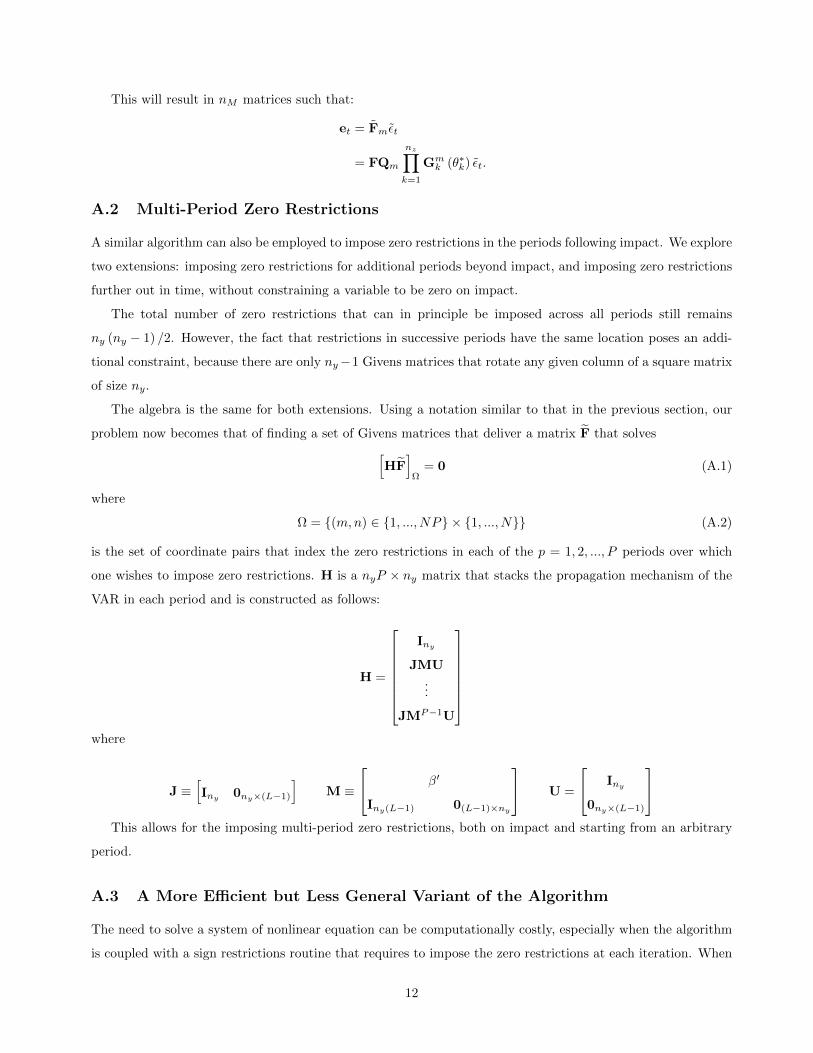
A.2 Multi-Period Zero Restrictions

A similar algorithm can also be employed to impose zero restrictions in the periods following impact. We explore

two extensions: imposing zero restrictions for additional periods beyond impact, and imposing zero restrictions

further out in time, without constraining a variable to be zero on impact.

The total number of zero restrictions that can in principle be imposed across all periods still remains

ny (ny − 1) /2. However, the fact that restrictions in successive periods have the same location poses an addi-

tional constraint, because there are only ny−1 Givens matrices that rotate any given column of a square matrix

of size ny.

The algebra is the same for both extensions. Using a notation similar to that in the previous section, our

problem now becomes that of finding a set of Givens matrices that deliver a matrix F that solves[HF

]Ω

= 0 (A.1)

where

Ω = (m,n) ∈ 1, ..., NP × 1, ..., N (A.2)

is the set of coordinate pairs that index the zero restrictions in each of the p = 1, 2, ..., P periods over which

one wishes to impose zero restrictions. H is a nyP × ny matrix that stacks the propagation mechanism of the

VAR in each period and is constructed as follows:

H =

Iny

JMU...

JMP−1U

where

J ≡[Iny

0ny×(L−1)

]M ≡

β′

Iny(L−1) 0(L−1)×ny

U =

Iny

0ny×(L−1)

This allows for the imposing multi-period zero restrictions, both on impact and starting from an arbitrary

period.

A.3 A More Efficient but Less General Variant of the Algorithm

The need to solve a system of nonlinear equation can be computationally costly, especially when the algorithm

is coupled with a sign restrictions routine that requires to impose the zero restrictions at each iteration. When

12

there are only relatvely few restrictions, and subject to some feasibility constraints, there is an alternative to

step 2 the algorithm described in the main text which doesn’t require the joint solution of a system of equations,

but instead works recursively.

The following example illustrates how this alternative algorithm works. As before, the goal is to find m

identified structures Fm which satisfy

Fmεt = et

and suppose we wanted to set two elements of Fm equal to zero on impact:

Ω = (3, 1) , (1, 3)

Recall that a Givens matrix solves the following problem:

G

ab

=

c0

and let us again start from the Cholesky decomposition of Σ, F, post-multiplied by an orthonormal matrix

Q.

We can impose [FQ]31 = 0 using the second column of FQ as a “pivot”, by solving:g111 g1

12

g121 g1

22

[FQ]32

[FQ]31

=

c0

and then post-multiplying FQ as follows:

FQG1 = FQ

g1

11 g112 0

g121 g1

22 0

0 0 1

Similarly, [FQG1]13 = 0 can be imposed by solving:

g211 g2

12

g221 g2

22

[FQG1]32

[FQG1]31

=

c0

and then postmultiplying by G2 =

1 0 0

0 g211 g2

12

0 g221 g2

22

.

Thus,

Fm = FQmGm1 Gm

2 .

Several things should be noted. First of all, the algorithm is recursive: G2 is computed on the basis of the

postmultiplied matrix FG1, where one zero restriction had already been imposed. This is possible because a

Givens rotation only affects two rows and columns of a matrix, so the first restriction is preserved when we

13

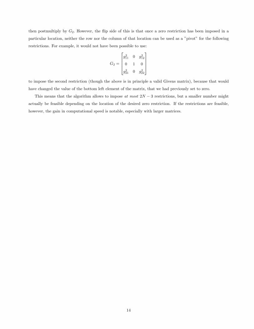
then postmultiply by G2. However, the flip side of this is that once a zero restriction has been imposed in a

particular location, neither the row nor the column of that location can be used as a ”pivot” for the following

restrictions. For example, it would not have been possible to use:

G2 =

g2

11 0 g212

0 1 0

g221 0 g2

22

to impose the second restriction (though the above is in principle a valid Givens matrix), because that would

have changed the value of the bottom left element of the matrix, that we had previously set to zero.

This means that the algorithm allows to impose at most 2N − 3 restrictions, but a smaller number might

actually be feasible depending on the location of the desired zero restriction. If the restrictions are feasible,

however, the gain in computational speed is notable, especially with larger matrices.

14