Contents lists available at ScienceDirect

Applied Energy

journal homepage: www.elsevier.com/locate/apenergy

Estimating ramping requirements with solar-friendly flexible rampingproduct in multi-timescale power system operations

Mingjian Cui, Jie Zhang⁎

Department of Mechanical Engineering, The University of Texas at Dallas, Richardson, TX 75080, USA

H I G H L I G H T S

• A multi-timescale unit commitment and economic dispatch model is developed to estimate the ramping requirements.

• A solar power ramping product (SPRP) is developed and integrated into the multi-timescale dispatch model.

• A surrogate-based optimization model is developed to solve the ramping requirements problem.

• SPRP can reduce the total cost of flexible ramping reserves.

A R T I C L E I N F O

Keywords:Economic dispatchLatin hypercube samplingPhotovoltaic (PV)Flexible ramping capabilityFlexibilityUnit commitment

A B S T R A C T

The increasing solar power penetration causes the need of additional flexibility for power system operations.Market-based flexible ramping services have been proposed in several balance authorities to address this issue.However, the ramping requirements in multi-timescale power system operations are not well defined and stillchallenging to be accurately estimated. To this end, this paper develops a multi-timescale unit commitment andeconomic dispatch model to estimate the ramping requirements. Furthermore, a solar power ramping product(SPRP) is developed and integrated into the multi-timescale dispatch model that considers new objectivefunctions, ramping capacity limits, active power limits, and flexible ramping requirements. To find the optimalramping requirement based on the level of uncertainty in netload, a surrogate-based optimization model isdeveloped to approximate the objective function of the multi-timescale dispatch model that considers botheconomic and reliability benefits of the balancing authorities. Numerical simulations on a modified IEEE 118-bussystem show that a better estimation of ramping requirements could enhance both the reliability and economicbenefits of the system. The use of SPRP can reduce the flexible ramping reserves provided by conventionalgenerators.

1. Introduction

Renewable energy is significantly impacting the economic and re-liable operations of the power systems, especially with the rapid in-crease of renewable penetration [1–3]. As an important renewablesource, solar power in the electric power grid rises continuously. Due tothe effects of microclimates (e.g., solar irradiance, temperature, andpassing clouds), solar power ramps occur frequently [4,5]. These solarpower ramps, in addition to the uncertainty and variability of solarpower, present new challenges to the balancing authorities. Multipleindependent system operators (ISOs) have proposed a flexible rampingproduct to help improve the dispatch flexibility to integrate thesevariable and uncertain renewables such as wind and solar [6–8].

Recently, wind has been proposed to provide ramping service for

the flexible operations of the power system [9–11], which also makessolar possible for balancing authorities to provide a solar-friendlyramping product in a similar manner. Solar power ramping product(SPRP) is essentially different from wind power ramping product(WPRP) that can be provided by any significant wind power ramp.SPRP should be provided by actual solar power ramp events (not due todiurnal pattern) that are caused by changes in short-term micro-cli-mates. In addition, SPRP could potentially reduce the production costby reducing the ramping reserve requirement provided by conventionalthermal generators, and also possibly enhance the reliability of powersystem operations. Thus in this paper, we are exploring the capability ofsolar to provide such flexibility service, and also evaluating the valuesof solar-friendly flexible ramping product in terms of the reliability andeconomic benefits for power system operations [12,13].

https://doi.org/10.1016/j.apenergy.2018.05.031Received 11 November 2017; Received in revised form 30 March 2018; Accepted 5 May 2018

⁎ Corresponding author.E-mail address: jiezhang@utdallas.edu (J. Zhang).

Applied Energy 225 (2018) 27–41

0306-2619/ © 2018 Elsevier Ltd. All rights reserved.

T

Nomenclature

Acronyms

SPRP solar power ramping productISO independent system operatorWPRP wind power ramping productMISO midcontinent independent system operatorCAISO California independent system operatorFESTIV flexible energy scheduling tool for integration of variable

generationDU day-ahead security-constrained unit commitmentRU real-time security-constrained unit commitmentRE real-time security-constrained economic dispatchAGC automatic generation controlOpSDA optimized swinging door algorithmFRP flexible ramping productMILP mixed-integer linear programmingACE area control errorCPS2 control performance standard 2NERC North American electric reliability corporationAACEE absolute area control error in energyKA Kriging approximationLHS Latin hypercube sampling

Parameters

t τ, indexes for time intervalsT (·) number of time periods. =T 4RU with 15-min time re-

solution in RU model and =T 3RE with 5-min time re-solution in RE model

NI number of thermal unitsNS number of solar generatorsNB number of busesCi

t(·)operation cost of thermal unit i during period tRU and tRE,in $

Sit(·)

start-up cost of thermal unit i during period tRU and tRE, in$

γi t,up

(·) , γi t,dn

(·) bidding price of flexible up/down ramping reserves of

thermal unit i during period tRU and tRE, in $/MWhps

t(·)power output of solar generator s at the end of period tRU

and tRE, in MWPi

min, Pimaxminimum/maximum generation of thermal unit i

dbt(·)

expected load of bus b at time t (·), in MWPLmax vector of power limit for transmission linesD vector of expected load or demandKP, KS, KD bus-thermal unit, bus-solar unit, and bus-load incidence

matricesP, PS vector of thermal dispatch and PV generationSF shift factor matrixXi

t,on(·), Xi

t,off(·)ON/OFF time of thermal unit i at time t (·)

Ti,on, Ti,off minimum ON/OFF time limits of unit iRi

up, Ridn maximum up/down ramping rate of thermal unit i, in

MW/minLC a sufficient large constantUPs

t(·), DPs

t(·)up/down solar power ramping product of solar gen-

erator s during period tRU and tRE, in MWURRt(·) total flexible upward ramping reserve requirements during

period tRU and tRE, in MWDRRt(·) total flexible downward ramping reserve requirements

during period tRU and tRE, in MW

m, n index of time points in the solar power dataR (·) ramp rule for measured or forecasted solar powerC (·) natural ramp rule for the clear-sky solar powerp s

tC,

(·)solar power generation in clear sky

ptNL actual netload at time t

+pt t5min|NL forecasted netload for the next 5min at time t

+pt t15min|NL forecasted netload for the next 15min at time t

σt,5min standard deviation of netload in the RE modelσt,15min standard deviation of netload in the RU modelλe, λr penalty multipliers for the economic and reliability bene-

fitsα, α minimum/maximum values of times of the standard de-

viation of netload in RE modelβ, β minimum/maximum values of times of the standard de-

viation of netload in RU modelx , μx, σx variable to be normalized, its mean value, and standard

deviationACEt inst, instantaneous ACE value at time period tTn, K1, K2 parameters used for the smoothed AGC modeφ(·) sensitivity coefficientsIRTD, HRTDtime resolution and horizon of the RE modelPWIND, PLOAD amount of wind power and load on the systemPRAMP amount of total ramping available from the resources to

manage the variabilityTCPS2 CPS2 interval, i.e., 10minΛ coefficient vector containing all the regression parameters

and = …λ λΛ [ , , ]1 6T

q, NS index and total number of sampled points (αq, βq)λ(·), θ, ω parameters of the KA modelμα, μβ mean values of sampled αq and βqσα, σβ standard deviations of sampled αq and βq

Variables and Functions

pit(·)

dispatch of thermal unit i at the end of period tRU and tRE,in MW

uit(·)

1 if unit i is scheduled on during period tRU and tRE; and 0otherwise

fuit(·), fdi

t(·)scheduled flexible up/down ramping reserves of thermal

unit i during period tDU, tRU, and tRE, in MWα, β times of the standard deviation of netload in RU and RE

modelsαN, βN normalized times of the standard deviation of netload in

RU and RE modelsS (·)c positive score function used in the dynamic programmingf (·) multi-objective function for obtaining reliability benefits

and minimizing dispatching costf α β( , ) Kriging approximation surrogate modelf [·]E functional relationship between the economic metrics and

times of standard deviationf [·]R functional relationship between the reliability metrics and

times of standard deviation(·)F realization function of a regression model in KA(·)R correlation function in KA

α βf( , ) polynomial function vector set containing polynomials oforders 0, 1, and 2: =α β α β α α β βf( , ) [1, , , , , ]N N N

2N N N

2

∇f (·) gradient matrix of KAH f( (·)) Hessian matrix of KAρ control factor used to limit the provision of SPRP

p tESS

(·)charged power of ESS at time t (·)

M. Cui, J. Zhang Applied Energy 225 (2018) 27–41

28

Currently, both the Midcontinent Independent System Operator(MISO) and California Independent System Operator (CAISO) havedesigned the ramping product to manage netload variations and un-certainties to maintain power balance in the real-time dispatch process[6,7,14]. Ramping products are defined at different real-time operationtimescales, which should be secured five, ten, or fifteen minutes aheadbased on the ISO’s market rules. Both the 5-min and 10-min aheadramping products can be sequentially integrated into the economicdispatch cycles run at a 5-min or 10-min time resolution. The 15-minahead ramping products can be sequentially integrated into the real-time unit commitment cycles run at a 15-min time resolution. Themarket schemes and operation scales vary among different ISOs. Abalance authority may only have 5-, 10-, or 15-min markets, but un-likely have all of them. In this paper, we only consider the 5- and 15-min ahead ramping products in the market scheme.

To effectively evaluate the impacts of solar power on the flexibleramping products, it is important to first accurately estimate theramping requirements in power system operations. Currently, rampingrequirements can be divided into soft and hard methods varying withthe method of capturing the system-wide ramping capacity [15]. Thesoft method utilizes the demand curve to price the ramping capabilityviolation and considers ramping requirements as decision variablesadded to both the objective function and constraints. The hard methodconsiders ramping requirements as given values, based on the varia-bility from the current dispatch interval to a future interval and theuncertainty at a future interval. MISO proposed a Gaussian-sigma rulebased on the Gaussian distribution [7]. The ramping requirement wasset as the netload variations plus the standard deviation of netloadforecasting errors. Wang et al. [14] proposed a simulation-basedmethod to determine the level of uncertainty in netload based on theMISO market rules from the perspective of reliability. To extend thework in [14], it would be interesting to optimally determine the level ofuncertainty in netload by considering both the economic and reliabilityperformance in power system operations. In addition, though multi-timescale power system operations have been progressed in recentyears [11,16–18], few studies have focused on estimating ramping re-serve requirements in a multiple timescales manner to ensure a realisticstudy.

Furthermore, the ramping requirement will be varying with theincrease of solar power penetration. With the continuous improvementof solar forecasting accuracy, it is possible to use solar power to provideflexible ramping reserves in the future. Thus, it would also be inter-esting to study the impacts of solar-friendly flexible ramping product onestimating the ramping reserves provided by conventional thermalgenerators. To this end, this paper aims to design and integrate a solarpower ramping product in multi-timescale power system operations,

and to estimate the flexible ramping requirements by considering boththe economic and reliability benefits in power system operations. Themain innovations and contributions of this paper include: (i) developinga novel ramping requirements estimation method by using the surro-gate-based optimization model; (ii) designing SPRPs by transformingnegative characteristics of SPRPS into advantageous ones; and (iii)analyzing the impact of SPRPs on estimating ramping requirements ofpower system optimization models.

The organization of this paper is as follows. In Section 2, a modifiedmulti-timescale scheduling model that considers the solar-friendlyflexible ramping product and ramping requirement estimation is de-veloped. Section 3 presents a developed surrogate-based optimizationmodel to approximate the power system operations by simultaneouslyquantifying the economic and reliability metrics. Case studies and re-sults analysis performed on a modified IEEE 118-bus system are dis-cussed in Section 4. The controllability of SPRP is discussed in Section5. Concluding remarks and future work are given in Section 6.

2. Multi-timescale scheduling models

To estimate the ramping requirement for power system operations,we use a multi-timescale scheduling method based on a simulation tool,Flexible Energy Scheduling Tool for Integration of Variable Generation(FESTIV) [16,19], as illustrated in Fig. 2. Four power system operationsub-models are included in FESTIV, including day-ahead security-con-strained unit commitment (DU), real-time security-constrained unitcommitment (RU), real-time security-constrained economic dispatch(RE), and automatic generation control (AGC), as shown in the leftblock of Fig. 2. The details of these sub-models are discussed in Sections2.1 and 2.2. SPRP is designed and considered in each dispatch stage,which is integrated into FESTIV through a solar power ramp detectionmethod, the optimized swinging door algorithm (OpSDA), as shown inthe right block of Fig. 2. The details of OpSDA are discussed in Section2.3. Ramping requirement estimation is discussed in Section 2.4.

The temporal coupling of sub-models is important because theconfigurable timing parameters will ensure a realistic study. Fig. 1shows how the four sub-models are coupled with different timeframes.In this figure, I represents the interval length, t represents the timebetween updates, and H represents the scheduling horizon. For the DUsub-model, the interval resolution is IDU (1 h). DU is simulated every tDU(24 h) which is usually once per day in the current operation system.The optimization horizon (HDU) in DU is 24 h (one day). The RU sub-model is repeated every tRU (15min) at an interval resolution of IRU(15min) and an optimization horizon of HRU (45min). The RE sub-model is repeated every tRE (5 min) at an interval resolution of IRE

(5 min) and an optimization horizon of HRE (10min). The AGC sub-

Fig. 1. Timeframes of FESTIV with four sub-models.

M. Cui, J. Zhang Applied Energy 225 (2018) 27–41

29

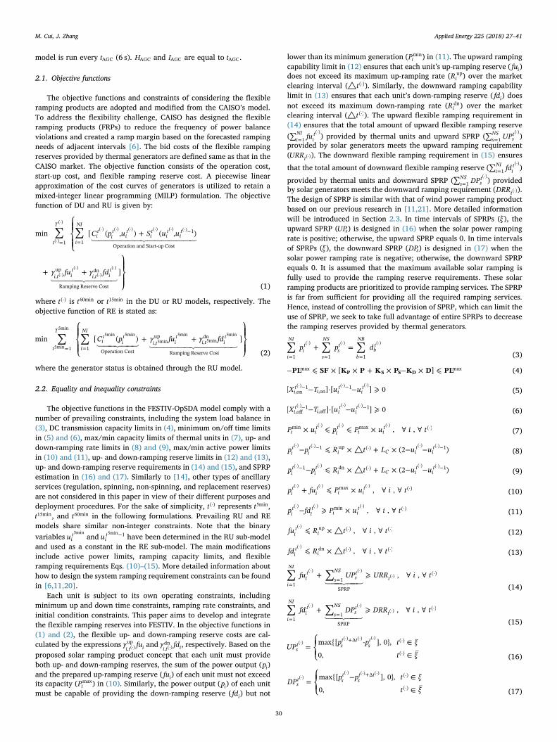
model is run every tAGC (6 s). HAGC and IAGC are equal to tAGC.

2.1. Objective functions

The objective functions and constraints of considering the flexibleramping products are adopted and modified from the CAISO’s model.To address the flexibility challenge, CAISO has designed the flexibleramping products (FRPs) to reduce the frequency of power balanceviolations and created a ramp margin based on the forecasted rampingneeds of adjacent intervals [6]. The bid costs of the flexible rampingreserves provided by thermal generators are defined same as that in theCAISO market. The objective function consists of the operation cost,start-up cost, and flexible ramping reserve cost. A piecewise linearapproximation of the cost curves of generators is utilized to retain amixed-integer linear programming (MILP) formulation. The objectivefunction of DU and RU is given by:

∑ ∑⎧

⎨⎪

⎩⎪+

+ +⎫

⎬⎪

⎭⎪

= =

−C p u S u u

γ fu γ fd

min [ ( , ) ( , )

]

t

T

i

NI

it

it

it

it

it

it

i t it

i t it

1 1

1

Operation and Start-up Cost

,up

,dn

Ramping Reserve Cost

(·)

(·)(·) (·) (·) (·) (·) (·)

(·)(·)

(·)(·)

(1)

where t (·) is t60min or t15min in the DU or RU models, respectively. Theobjective function of RE is stated as:

∑ ∑⎧

⎨⎪

⎩⎪+ +

⎫

⎬⎪

⎭⎪= =

C p γ fu γ fdmin [ ( ) ]t

T

i

NI

it

it

i t it

i t it

1 1 Operation Cost,up

,dn

Ramping Reserve Cost5min

5min5min 5min

5min5min

5min5min

(2)

where the generator status is obtained through the RU model.

2.2. Equality and inequality constraints

The objective functions in the FESTIV-OpSDA model comply with anumber of prevailing constraints, including the system load balance in(3), DC transmission capacity limits in (4), minimum on/off time limitsin (5) and (6), max/min capacity limits of thermal units in (7), up- anddown-ramping rate limits in (8) and (9), max/min active power limitsin (10) and (11), up- and down-ramping reserve limits in (12) and (13),up- and down-ramping reserve requirements in (14) and (15), and SPRPestimation in (16) and (17). Similarly to [14], other types of ancillaryservices (regulation, spinning, non-spinning, and replacement reserves)are not considered in this paper in view of their different purposes anddeployment procedures. For the sake of simplicity, t (·) represents t5min,t15min, and t60min in the following formulations. Prevailing RU and REmodels share similar non-integer constraints. Note that the binaryvariables ui

t5minand −ui

t 15minhave been determined in the RU sub-model

and used as a constant in the RE sub-model. The main modificationsinclude active power limits, ramping capacity limits, and flexibleramping requirements Eqs. (10)–(15). More detailed information abouthow to design the system ramping requirement constraints can be foundin [6,11,20].

Each unit is subject to its own operating constraints, includingminimum up and down time constraints, ramping rate constraints, andinitial condition constraints. This paper aims to develop and integratethe flexible ramping reserves into FESTIV. In the objective functions in(1) and (2), the flexible up- and down-ramping reserve costs are cal-culated by the expressions γ fu

i t i,up

(·) and γ fdi t i,dn

(·) , respectively. Based on theproposed solar ramping product concept that each unit must provideboth up- and down-ramping reserves, the sum of the power output (pi)and the prepared up-ramping reserve ( fui) of each unit must not exceedits capacity (Pi

max) in (10). Similarly, the power output (pi) of each unitmust be capable of providing the down-ramping reserve ( fdi) but not

lower than its minimum generation (Pimin) in (11). The upward ramping

capability limit in (12) ensures that each unit’s up-ramping reserve ( fui)does not exceed its maximum up-ramping rate (Ri

up) over the marketclearing interval (△t (·)). Similarly, the downward ramping capabilitylimit in (13) ensures that each unit’s down-ramping reserve ( fdi) doesnot exceed its maximum down-ramping rate (Ri

dn) over the marketclearing interval (△t (·)). The upward flexible ramping requirement in(14) ensures that the total amount of upward flexible ramping reserve(∑ = fui

NIit

1(·)) provided by thermal units and upward SPRP (∑ = UPs

NSst

1(·))

provided by solar generators meets the upward ramping requirement(URRt(·)). The downward flexible ramping requirement in (15) ensures

that the total amount of downward flexible ramping reserve (∑ = fdiNI

it

1(·))

provided by thermal units and downward SPRP (∑ = DPsNS

st

1(·)) provided

by solar generators meets the downward ramping requirement (DRRt(·)).The design of SPRP is similar with that of wind power ramping productbased on our previous research in [11,21]. More detailed informationwill be introduced in Section 2.3. In time intervals of SPRPs (ξ ), theupward SPRP (UPs) is designed in (16) when the solar power rampingrate is positive; otherwise, the upward SPRP equals 0. In time intervalsof SPRPs (ξ ), the downward SPRP (DPs) is designed in (17) when thesolar power ramping rate is negative; otherwise, the downward SPRPequals 0. It is assumed that the maximum available solar ramping isfully used to provide the ramping reserve requirements. These solarramping products are prioritized to provide ramping services. The SPRPis far from sufficient for providing all the required ramping services.Hence, instead of controlling the provision of SPRP, which can limit theuse of SPRP, we seek to take full advantage of entire SPRPs to decreasethe ramping reserves provided by thermal generators.

∑ ∑ ∑+ == = =

p p di

NI

it

s

NS

st

b

NB

bt

1 1 1

(·) (·) (·)

(3)

− ⩽ × × + × − × ⩽PL SF K P K P K D PL[ ]P S S Dmax max (4)

− − ⩾− −X T u u[ ]·[ ] 0it

i it

it

,on1

,on1(·) (·) (·)

(5)

− − ⩾− −X T u u[ ]·[ ] 0it

i it

it

,off1

,off1(·) (·) (·)

(6)

× ⩽ ⩽ × ∀ ∀P u p P u i t, ,i it

it

i itmin max (·)(·) (·) (·)

(7)

− ⩽ × △ + × − −− −p p R t L u u(2 )it

it

i C it

it1 up (·) 1(·) (·) (·) (·)

(8)

− ⩽ × △ + × − −− −p p R t L u u(2 )it

it

i C it

it1 dn (·) 1(·) (·) (·) (·)

(9)

+ ⩽ × ∀ ∀p fu P u i t, ,it

it

i itmax (·)(·) (·) (·)

(10)

− ⩾ × ∀ ∀p fd P u i t, ,it

it

i itmin (·)(·) (·) (·)

(11)

⩽ × △ ∀ ∀fu R t i t, ,it

iup (·) (·)(·)

(12)

⩽ × △ ∀ ∀fd R t i t, ,it

idn (·) (·)(·)

(13)

∑ ∑+ ⩾ ∀ ∀=

=fu UP URR i t, ,

i

NI

it

s

NSst

t1

1

SPRP

(·)(·) (·)(·)

(14)

∑ ∑+ ⩾ ∀ ∀=

=fd DP DRR i t, ,

i

NI

it

s

NSst

t1

1

SPRP

(·)(·) (·)(·)

(15)

=⎧⎨⎩

∈

∈

+UP p p t ξ

t ξ

max{[ - ], 0},

0,st s

t tstΔ (·)

(·)

(·)(·) (·) (·)

(16)

=⎧⎨⎩

− ∈

∈

+DP p p t ξ

t ξ

max{[ ], 0},

0,st s

tst tΔ (·)

(·)

(·)(·) (·) (·)

(17)

M. Cui, J. Zhang Applied Energy 225 (2018) 27–41

30

2.3. Solar power ramping products detected by dynamic programming

Ramps in solar power consist of natural ramps and actual rampevents. The distinctions between natural ramps and actual ramp eventscan be explained from two perspectives: physical phenomenon andpower system operations. From the perspective of physical phenom-enon, natural ramps is expected to occur in both the actual solar powergeneration and the clear-sky power generation. The occurrence ofnatural ramps is due to the diurnal pattern of solar radiation. Actualramp events (not due to diurnal pattern) are caused by changes in short-term micro-climates, such as passing clouds [22]. From the perspectiveof power system operations, both natural and actual solar ramps can bemanaged by the flexible ramping reserve provided by thermal units.This concept has been designed by both MISO and CAISO [6,7,14].However, the actual ramp events can be additionally used in this paperto take advantage of their negative characteristics, i.e., large fluctua-tions (significant increase or decrease) of solar power in a short timeperiod. Hence, the negative characteristic of actual solar power rampevents can be transformed into an advantageous one as the SPRP. Underthis circumstance, this paper assumes that only actual solar power rampevents provide SPRP. Note that using natural ramps to provide SPRP isbeyond the scope of this paper, which can be studied in the future. Inthe current market, the ramping product can only be represented bygeneration output difference between two successive time intervals.While in our developed ramping product model, SPRPs are provided inthe time intervals when the upward and downward solar power rampevents occur (rather than successive time intervals). This model hasbeen successfully used for the design of wind power ramping product,more detailed information on which can be found in [11,21].

Hence, SPRPs are defined as those ramp events that occur in theactual solar power generation however not in the clear-sky powergeneration. After identifying all significant ramps in the measured orforecasted solar power generation, the clear-sky solar ramps are re-moved as natural ramps that are caused by the diurnal pattern of solarradiation. First, the solar power data is segregated by the OpSDA [23]with a predefined compression deviation ε. Then all extracted segmentsare input into the dynamic programming (the light blue block in Fig. 2)and merged to yield a set of SPRPs. Designed as positive characteristicsof solar power ramps, the SPRP is integrated into the multi-timescaledispatch model that considers new objective functions, ramping capa-city limits, active power limits, and flexible ramping requirements. Apositive score function Sc is used in the dynamic programming to detectall SPRPs, given by:

= − × − ×S m n m n C m n R m n( , ) ( ) [1 ( , )] ( , )c2 (18)

= ⎧⎨⎩

− >− ⩽

R m np pp p

( , )1, if | | 0.15 p.u.0, if | | 0.15 p.u.

sm

sn

sm

sn

(19)

= ⎧⎨⎩

− >

− ⩽C m n

p p

p p( , )

1, if | | 0.15 p.u.

0, if | | 0.15 p.u.s

ms

n

sm

sn

C, C,

C, C, (20)

where =R m n( , ) 1 when a ramp occurs in the measured or forecastedsolar power. =C m n( , ) 1 when a natural ramp occurs in the clear-skygeneration. Both R m n( , ) and C m n( , ) are defined as the change in solarpower magnitude without the ramping duration limit [23–25].

In this paper, the change in solar power output is set to be greaterthan 15% of the installed capacity of solar generators (i.e., 0.15 p.u.).Due to the diurnal pattern of solar power, the aim of (18) is to assurethe design of a true SPRP. The OpSDA combines the adjacent segmentsin the same direction and detects SPRPs by removing those occurring inthe clear-sky power generation. A more detailed description of OpSDAcan be found in [22,23].

As shown in Fig. 3, the natural upward ramp spans from 8:00 to10:00 and the natural downward ramp spans from 15:00 to 17:00.

These two natural ramps occur due to the diurnal pattern of solar ra-diation and are not used to design the SPRP. In order to transform anegative characteristic of solar power ramp event into an advantageousone, the upward ramp event spanning from 13:00 to 14:00 and thedownward ramp event spanning from 14:00 to 14:30 are used to designthe SPRP in this paper. Differently with thermal units, solar power canonly provide SPRPs when actual ramps occur. Taking the time intervalspanning from 10:00 to 13:00 as an example, the slight solar powergeneration output difference (sometimes even approximately equal 0)in successive time intervals could not be used to provide a satisfactoryamount of SPRPs.

2.4. Ramping reserve requirement estimation

Different methodologies have been used to define the ramping re-serve requirements. For example, MISO designs the ramping reserverequirements by assuming that the uncertain netload follows a Gaussiandistribution and utilizes the level of uncertainty based on a Gaussian-sigma rule, where the uncertainty is represented by the standard de-viation of the netload [7]. The netload is defined as the load demandminus the renewable energy sources from solar power [7,14,26,27]. Forthe RE model, the amount of upward ramping reserve requirementURRt

RE is set as the variation between the forecasted netload +pt t5min|NL

and the actual netload ptNL plus ‘α’ times of the standard deviation [14],

given by:

= − ++URR p p ασmax{0, }t t t t tRE

5min|NL NL

,5min (21)

Symmetrically, the amount of downward ramping reserve

Fig. 2. Multi-timescale scheduling model based on FESTIV and OpSDA.

M. Cui, J. Zhang Applied Energy 225 (2018) 27–41

31

requirement DRRtRE is set as the variation between the forecasted net-

load +pt t5min|NL and the actual netload pt

NL minus ‘α’ times of the standarddeviation, given by:

= − ++DRR p p ασmax{0, }t t t t tRE NL

5min|NL

,5min (22)

In this paper, we also utilize the ramping reserve requirement de-fined in the RE model and further extend it to the RU model. Similarly,the amount of upward ramping reserve requirementURRt

RU in RU is setas the variation between the forecasted netload +pt t15min|

NL and the actualnetload pt

NL plus ‘β’ times of the standard deviation:

= − ++URR p p βσmax{0, }t t t t tRU

15min|NL NL

,15min (23)

where σt,15min is approximated by the total probability theory as=σ σ3t t,15min ,5min for Gaussian distribution [28].

Symmetrically, the amount of downward ramping reserve require-ment DRRt

RU in RU is set as the variation between the forecasted net-load +pt t15min|

NL and the actual netload ptNL minus ‘β’ times of the standard

deviation, given by:

= − ++DRR p p βσmax{0, }t t t t tRU NL

15min|NL

,15min (24)

By optimally determining the values of α and β, the ramping re-quirements of both RE and RU models can hence be estimated with theconsideration of both economic and reliability benefits. Thus, a multi-objective optimization model is developed, where both economic andreliability metrics ( f [·]E and f [·]R ) are represented as functions of themultipliers of standard deviations, i.e., α and β. However, these func-tions cannot be analytically expressed due to the complexity of powersystem operations. Thus in this paper, a surrogate model is developed toapproximate the multi-timescale power system scheduling models,which is described in Section 3. In addition, most of current literaturesonly consider the economic benefits by minimizing the total dis-patching cost in the RE timescale. The multi-objective function devel-oped in this paper also minimizes the system’s area control error (ACE)to obtain the reliability benefits in both RE and RU timescales, given by:

=

+ ⩽ ⩽ ⩽ ⩽

f α β λ f RR α RR β

λ f RR α RR β α α α β β β

min ( , ) · [ ( ), ( )]

· [ ( ), ( )], ,

e E t t

r R t t

,5minRE

,15minRU

,5minRE

,15minRU

(25)

where the initial ranges of α and β are determined by heuristics as [α,α] and [β, β ], respectively [14]. λe and λr are penalty multipliers thatcan be selected based on the preference of balancing authorities. f [·]Erepresents the functional relationship between the economic metricsand (α, β). f [·]R represents the functional relationship between thereliability metrics and (α, β). A detailed description of economic andreliability metrics is provided in the following section. Due to the scaledifference, both the economic and reliability metrics are normalized asfollows:

= −x x μ σ( )/x xN (26)

where x is the variable to be normalized. μx and σx are the mean value

and standard deviation of multiple samples, respectively.

2.5. Economic and reliability metrics

The total power system production cost is directly computed by theFESTIV-OpSDA model. The cost of each generator to supply energy atevery AGC interval for the entire study period is calculated. This in-cludes the start-up, no-load, and incremental energy cost, as well as anybid in flexible ramping reserve costs. The economic profit is the revenueminus the total cost of all generation resources. The revenue is the totalrevenue of all generation resources in the system after getting paid thelocational marginal price for energy and any ancillary service price forancillary service provisions.

Reliability metrics are calculated based on the system’s ACE and theControl Performance Standard 2 (CPS2) proposed by the NorthAmerican Electric Reliability Corporation (NERC) [29,30]. ACE is thedifference between the sum of total generation and load at any time,which is the main driver of all imbalance metrics, give by:

∫= +−

ACE K ACE KT

ACE dτt t instn t T

tτ inst1 ,

2,

n (27)

where ACEt is the smoothed ACE value of the system at time period t.ACEt inst, represents the instantaneous ACE value at time period t. Theterm τ is the index for time intervals. The terms Tn, K1, and K2 areparameters used for the smoothed AGC mode.

Absolute area control error in energy (AACEE) is the absolute valueof ACE at every tAGC interval, where tAGC is the highest time resolution(in seconds) at which AGC is run. AACEE is a function of the time re-solution of the RE (IRTD), the time horizon of the RE (HRTD), the amountof wind power on the system (PWIND), the load (PLOAD), and the amountof total ramping available from the resources to manage the variability(PRAMP), formulated as:

= + + + +AACEE φ I φ H φ P φ P φ P1 RTD 2 RTD 3 WIND 4 LOAD 5 RAMP (28)

where φ is the sensitivity coefficient and can be calculated from thestandard deviation of output changes at different timescales, i.e.,

= ∂ ∂φ AACEE I/1 RTD; = ∂ ∂φ AACEE H/2 RTD; = ∂ ∂φ AACEE P/3 WIND;= ∂ ∂φ AACEE P/4 LOAD; and = ∂ ∂φ AACEE P/5 RAMP.CPS2 is a NERC reliability standard that measures the amount of

intervals where the absolute value of ACE exceeds a predefinedthreshold [31]. Based on CPS2, the reliability indicator ACECPS2 mea-sures the sum of instantaneous ACE until the 10-min CPS2 interval(L10) ends. Thus, the unit of ACECPS2 is MW-10min and the τ thACECPS2 is formulated as:

∑= ×= − × ×

× × −

ACE ACE tT60τ

t τ T

τ T t

t instCPS2,( 1) 60

60

,AGC

CPS2CPS2

CPS2 AGC

(29)

where TCPS2 is the CPS2 interval, i.e., 10min. τ is the index of the τ thACECPS2 value.

Overall, it should be noted that lower ACE, AACEE, and ACECPS2

Fig. 3. An example of solar power ramping product in one day.

M. Cui, J. Zhang Applied Energy 225 (2018) 27–41

32

indicate a better reliability performance. These metrics have beenwidely used in literature for the analysis of power system operations.Ela and O’Malley [16] calculated these reliability metrics to analyze theuncertainty impacts of wind power forecast errors. Ela et al. [32] alsoanalyzed the impacts of the netload variability with wind integrationbased on these reliability metrics calculated by ACE. Wang et al. [33]measured the reliability improvements by calculating ACE for improvedwind power forecasting. Cui et al. [11] found that the reliability ofpower system operations was enhanced with wind power rampingproducts by calculating ACE and corresponding reliability metrics.

3. Surrogate-based optimization

3.1. Surrogate model of multi-objective function

The Kriging surrogate model has been widely used in design andoptimization community [34–37]. It is used to provide approximationsof computationally expensive simulations and experiments. For ex-ample, Huang et al. [34] developed a design optimization methodbased on the Kriging surrogate model for the shape optimization of anaeroengine turbine disc. Song et al. [35] developed a Kriging surrogatemodel to design and optimize a plate-fin-type heat sink. Gao et al. [36]used a Kriging surrogate model to identify the optimal tip locations ofan internal crack in cantilever plates. Xia et al. [37] employed theKriging surrogate model in the finite element analysis to reduce thecomputing time for multi-objective robust optimization of electro-magnetic devices. The optimization problems in power system opera-tions are complex and generally computationally expensive, especiallyfor the multiple timescales power system operations studied in thispaper. Surrogate modeling such as Kriging is expected to reduce thecomputational burden significantly. In this paper, the ramping reserverequirements estimation problem makes it possible to use the Krigingsurrogate model for an optimal solution.

First, the economic and reliability metrics are calculated throughmulti-timescale power system operations (e.g., FESTIV-OpSDA), whichgenerally cannot be represented by straightforward mathematical

functions of “α” and “β” that determine the ramping requirements.Thus, to successfully integrate the multi-objective function in (25) intothe overall optimization problem, an approximation model needs to bedeveloped. To this end, surrogate modeling that is widely used in themultidisciplinary design optimization society [38], is adopted here toapproximate the f α β( , ) in (25) by replacing the complex power systemoperation simulations. Then, the optimization can be performed di-rectly based on the surrogate model. In this paper, a Kriging surrogatemodel is developed to approximate the objective f in (25) as a functionof ramping requirement design variables, α and β. A design and analysisof computer experiments [39] is performed based on the FESTIV-OpSDA platform. The Kriging approximation (KA) surrogate model,f α β( , ) , is established to formulate the deterministic response f α β( , ) in(25) with a two dimensional input, given by:

= + ≈ ⩽ ⩽ ⩽ ⩽f α β λ α β ω α β f α β α α α β β β( , ) ( ; , ) ( ; , ) ( , ) ,F R

(30)

where F is a realization function of a regression model, given by:

=λ α β α βf( ; , ) ( , )ΛF (31)

where α βf( , ) is a function vector set containing polynomials of orders 0,1, and 2, i.e., =α β α β α α β βf( , ) [1, , , , , ]N N N

2N N N

2 . The variables αN and βNrepresent the normalization of variables α and β, respectively, i.e.,

= −α α μ σ( )/α αN and = −β β μ σ( )/β βN . The coefficient vector Λ containsall the regression parameters, i.e., = …λ λΛ [ , , ]1 6

T. R is a correlationfunction, given by:

∑==

− − + −θ ω α β ω e( , ; , )q

N

qθ α α σ θ β β σ

1

[ ( ) / ( ) / ]α q α β q βS

2 2 2 2R

(32)

where (αq, βq) is sampled by the Latin hypercube sampling (LHS) [40]and used to simulate the objective f α β( , )q q in (25) using the FESTIV-OpSDA model. The total number of sampled points (αq, βq) is NS. The

mean values of (αq, βq) are expressed as = ∑ =μ αα N qN

q1

1SS and

= ∑ =μ ββ N qN

q1

1SS . The standard deviations of (αq, βq) are expressed as

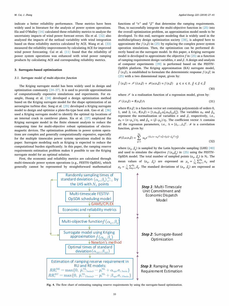
Fig. 4. The flow chart of estimating ramping reserve requirements by using the surrogate-based optimization.

M. Cui, J. Zhang Applied Energy 225 (2018) 27–41

33

= ∑ −=σ α μ( )α N qN

q α1

12

SS and = ∑ −=σ β μ( )β N q

Nq β

11

2S

S . All the para-

meters of the KA model (Λ, θ, and ω) are calculated by the generalizedleast squares estimate [41]. The optimization of the surrogate model(30) is solved by using the Newton’s method. The gradient, ∇f α β( , ) ,and Hessian matrix, H f α β( ( , )) , of the KA model are deduced in Ap-pendix A, respectively.

3.2. Procedure of estimating ramping reserve requirements

The flow chart of estimating ramping reserve requirements by usingthe surrogate-based modeling is shown in Fig. 4, which consists of threemajor steps: multi-timescale unit commitment and economic dispatchmodels, surrogate-based optimization, and ramping reserve require-ment estimation. The three major steps are described as follows:

• Step 1: Randomly sample times of standard deviation =α β( , )q q qN

1S by

using LHS with NS points. The corresponding ramping reserve re-quirements are determined by these samples (as described in Section2.4), and input into the multi-timescale FESTIV-OpSDA schedulingmodel (as described in Sections 2.1,2.3). Both economic and relia-bility metrics are then calculated, as described in Section 2.5.

• Step 2: The multi-objective function f α β( , ) that is calculated by theeconomic and reliability metrics, and the sampled times of standarddeviation α β( , ) are approximated by the surrogate-based optimiza-tion model, as described in Section 3.1. Then, the optimal α β( , )opt optis solved by the Newton’s method based on the gradient and Hessianmatrix.

• Step 3: The estimated ramping reserve requirements are finallydetermined by the variation between the forecasted and actualnetload plus ‘αopt’ or ‘βopt’ times of the standard deviation.

4. Case studies and results

4.1. Test cases

We perform numerical simulations on a modified IEEE 118-bussystem using the FESTIV-OpSDA platform. All tests are carried out byusing the General Algebraic Modeling System (GAMS) Distribution 24.7[42], and solved using ILOG CPLEX 12.6 [43] on two Intel-e5-2603 1.6-GHz workstations with 32 GB of RAM memory. This system has 54thermal units, 186 branches, and 91 load buses. The parameters ofgenerators, transmission network, and load profiles are given in[44,45]. The system peak demand is 4,064MW at the time stamp18:46:24. To present a more realistic renewable-based generationsystem, the IEEE 118-bus system (as shown in Fig. 5) is modified byallocating 10 solar generators with the same location in [11], based onthe apparent power of the loads and the distance of transmission lines.More detailed information about the allocation of solar generators canbe found in [33]. These 10 solar generators are integrated into threezones: (i) Bus 4, 26, and 27 in the top left zone; (ii) Bus 40, 49, and 62 inthe top right zone; and (iii) Bus 89, 100, 107, and 112 in the bottomright zone. SPRP is used to analyze the results of Sections 4.2, 4.3 and4.4. Section 4.5 compares the results with and without SPRP. Section4.6 compares the results with and without confidence levels.

Solar power data is collected from the Watt-sun forecasts [46].Watt-sun solar forecasting is developed based on a situation-dependentmulti-expert machine learning method, which combines the linearmodel, random forests, and support vector machine methods to en-hance the forecast accuracy. It leans on historical forecasts. A dozen ofsingle machine-learning models are set-up and ingest the multiple nu-merical weather prediction models for the situation dependentlearning. The algorithm that provides the best accuracy for the last twodays is selected for future solar power forecasts. Numerical results haveshown an approximately 30% improvement in solar irradiance/powerforecasting accuracy compared to forecasts based on the best individualmethod. Detailed information on the Watt-sun solar forecasting system

Fig. 5. The modified IEEE 118-bus system with 10 solar generators.

M. Cui, J. Zhang Applied Energy 225 (2018) 27–41

34

can be found in [46].Clear sky is a hypothetical field assuming no clouds. Clear-sky solar

power generation means the solar power generation that is directlyconverted from solar irradiance in this hypothetical clear-sky field. Thesolar irradiance data are collected from the Solar Resource &Meteorological Assessment Project (SOLRMAP) developed by theNational Renewable Energy Laboratory (NREL) [47]. Then the solarpower data is calculated through the collected solar irradiance data byusing the PV_LIB toolbox [48].

4.2. Simulation results

Fig. 6 shows the performance of the KA surrogate model and theconvergence history of obtaining the optimal multipliers of the stan-dard deviation in the modified IEEE 118-bus system. The approximatedKA model and corresponding MSEs are illustrated in Fig. 6(a) and (b),respectively. The estimated parameters of this surrogate model arelisted in Table 1 with a same penalty multiplier, = =λ λ 0.5e r . Theiterative process using the Newton’s method with multiple contours isshown in Fig. 6(c). It is shown that the optimal solution of the surro-gate-based optimization is obtained at the point =α 0.69min and

=β 1.26min . The optimization convergence history of multiple simula-tions using the LHS sampling method is shown in Fig. 6(d). It is ob-served that the optimal results are robust with respect to different LHSsamples. To validate the accuracy of the surrogate-based optimizationresults, a Monte-Carlo simulation is performed using the LHS samplingmethod with 10,000 runs, as shown in Fig. 7. The mean values of αoptand βopt are normally distributed around 0.69 and 1.26 with relativelysmall standard deviations 0.0163 and 0.0149, respectively.

The optimal results with different numbers of samples of α and β areillustrated in Fig. 8. It is seen when the number of samples is 22, we canget a relatively convergent optimum with and ≈β 1.26opt . It means thatthe total execution time could be approximatively reduced from 15 hwith 30 points to 11 h with 22 points (about 30min for one sample)with a satisfactory precision.

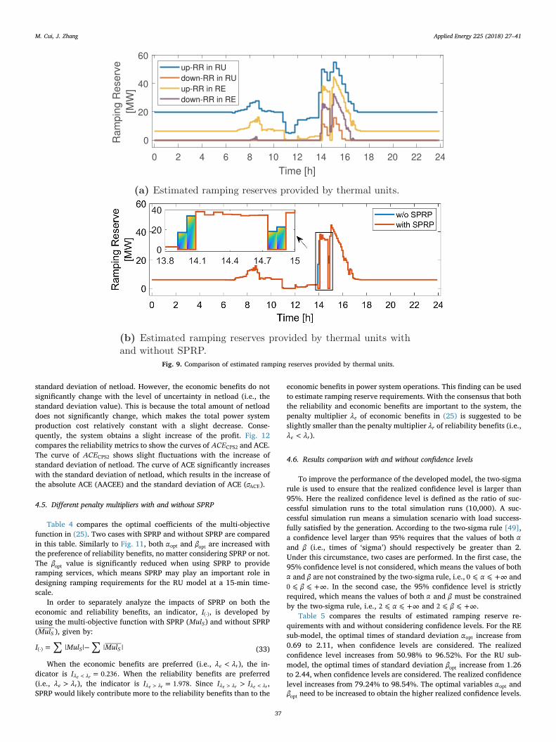
The results of ramping reserves provided by thermal units arecompared in Fig. 9. Fig. 9a compares the estimated up- and down-ramping reserves provided by thermal units in RU and RE models. Thetotal energy of up- and down-ramping reserves provided by thermalunits in the RE model is 251MWh, and the total energy of up- anddown-ramping reserves provided by thermal units in the RU model is538MWh. It is observed that the RE model requires less ramping

Fig. 6. Performance of the KA model and the convergence history of obtaining the optimal multipliers of the standard deviations using the Newton’s method.

Table 1Parameters of the KA model with penalty multipliers of = =λ λ 0.5e r .

λ1 λ2 λ3 λ4 λ5 λ6 θα θβ

−0.865 0.692 0.011 0.294 −0.013 0.632 1.250 1.249

ω1 ω2 ω3 ω4 ω5 ω6 ω7 ω80.351 0.057 1.501 0.495 0.167 −0.729 −0.189 −0.482

ω9 ω10 ω11 ω12 ω13 ω14 ω15 ω16−0.851 0.206 1.476 −0.881 −0.498 −0.111 −0.721 0.229

ω17 ω18 ω19 ω20 ω21 ω22 ω23 ω24−1.633 0.009 1.089 −0.741 0.072 4.267 0.967 6.223

ω25 ω26 ω27 ω28 ω29 ω30−5.911 −5.728 0.646 0.638 0.381 −0.303

M. Cui, J. Zhang Applied Energy 225 (2018) 27–41

35

reserves from thermal units than the RU model. This is mainly becausethe netload variation in RE (5-min time resolution) is less than that inRU (15-min time resolution). Fig. 9b compares the total estimatedramping reserves provided by thermal units with SPRP (the red line)and without SPRP (the blue line), which are 2431MW×5min and2523MW×5min, respectively. In this case, SPRP saves approximately3.63% [=(2523− 2431)/2523] of ramping reserves provided bythermal units. When the solar power penetration level increases, thissaving percentage is expected to increase accordingly.

To study the sensitivity of ramping reserves to the solar powerforecasting accuracy, solar power data with a small forecasting errorinterval from 6MW to 6MW is simulated. Fig. 10 shows how the solarpower forecasting accuracy impacts the total ramping reserves of thepower system. The solar power forecasts are generated using a pre-defined normally distributed error that is randomly added to the perfectsolar power forecast. The measured solar power which is called theperfect solar forecast is taken as the 100% accuracy. Based on the 100%accurate solar power, forecast errors are uniformly increased by apercentage (20%) to create other decreased forecasting accuracy sce-narios (i.e., 80%, 60%, 40%, 20%, and 0%). Probability distributionfunctions (PDFs) of forecasting errors are shown in Fig. 10a. b showsthat total ramping reserves of the system in different forecasting casesare generally not sufficiently scheduled compared to the perfect fore-casting case (100%), since SPRPs are overestimated by forecasts.

4.3. Accuracy validation of the surrogate-based optimization

Fig. 11 compares the optimization results with different penaltymultipliers. It is observed that when reliability benefits are preferredover economic benefits, i.e., <λ λr e in Case c3, both optimal α and βcoefficients are increased in RE and RU models, compared to Case c2when =λ λr e. It results in more ramping requirements scheduled

according to (21) and (23) to obtain more reliability benefits. Wheneconomic benefits are preferred over reliability benefits, i.e., <λ λe r inCase c1, both α and β coefficients are decreased, compared to Case c2when =λ λr e. Under this circumstance, less ramping reserve is sched-uled according to (21) and (23) to obtain more economic benefits. Thus,the ramping requirements estimation accurately reflects the preferenceof balancing authorities.

Table 2 compares the economic and reliability benefits by randomlyusing two sets of α and β values to the optimal solution with the samepenalty multiplier: = =λ λ 0.5e r , where all the metrics are normalizedby (26). The optimal values of =α 0.69opt and =β 1.26opt generate theminimum multi-objective value, −1.305, comparing to other α and βvalues. The increase of β in RU model significantly impacts economicmetrics comparing to reliability metrics, as shown in the left half ofTable 2. This is because reliability metrics are calculated at the AGCtimescale (6-s time resolution) from which the RU timescale (15-mintime resolution) difference is longer than the RE timescale (5-min timeresolution). In the right half of Table 2, the increase of α significantlyimpacts both economic and reliability metrics. When α increases from0.19 to 0.69, the economic metric increases by 12.62%, however thereliability metric decreases by 902.78%. The final aggregated multil-objective reaches to the minimum, −1.305.

4.4. Comparison of different standard deviations using the estimatedramping reserve requirements

Table 3 compares the reliability and economic metrics by randomlychoosing standard deviation values with the optimal coefficients:

=α 0.69 and =β 1.26 in Section 4.2. Smaller AACEE and σACE indicate abetter performance in terms of the reliability indicators. A higher profitand lower cost indicate a better performance in terms of the economicindicators. It is shown that both AACEE and σACE increase with the

Fig. 7. Optimal multipliers values of the standard deviation using the LHS method based on statistical analysis with 10,000 simulation runs. The mean values of αmin

and βmin are 0.69 and 1.26, respectively, and the standard deviations are 0.0163 and 0.0149, respectively.

Fig. 8. Optimal results with different number of training points of α and β.

M. Cui, J. Zhang Applied Energy 225 (2018) 27–41

36

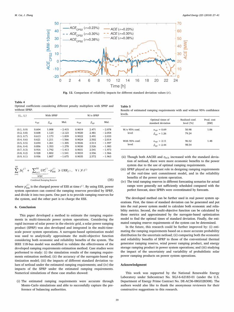
standard deviation of netload. However, the economic benefits do notsignificantly change with the level of uncertainty in netload (i.e., thestandard deviation value). This is because the total amount of netloaddoes not significantly change, which makes the total power systemproduction cost relatively constant with a slight decrease. Conse-quently, the system obtains a slight increase of the profit. Fig. 12compares the reliability metrics to show the curves of ACECPS2 and ACE.The curve of ACECPS2 shows slight fluctuations with the increase ofstandard deviation of netload. The curve of ACE significantly increaseswith the standard deviation of netload, which results in the increase ofthe absolute ACE (AACEE) and the standard deviation of ACE (σACE).

4.5. Different penalty multipliers with and without SPRP

Table 4 compares the optimal coefficients of the multi-objectivefunction in (25). Two cases with SPRP and without SPRP are comparedin this table. Similarly to Fig. 11, both αopt and βopt are increased withthe preference of reliability benefits, no matter considering SPRP or not.The βopt value is significantly reduced when using SPRP to provideramping services, which means SPRP may play an important role indesigning ramping requirements for the RU model at a 15-min time-scale.

In order to separately analyze the impacts of SPRP on both theeconomic and reliability benefits, an indicator, I(·), is developed byusing the multi-objective function with SPRP (MulS) and without SPRP(MulS ), given by:

∑ ∑= −I Mul Mul| | | |S S(·) (33)

When the economic benefits are preferred (i.e., <λ λe r), the in-dicator is =<I 0.236λ λe r . When the reliability benefits are preferred(i.e., >λ λe r), the indicator is =>I 1.978λ λe r . Since >> <I Iλ λ λ λe r e r ,SPRP would likely contribute more to the reliability benefits than to the

economic benefits in power system operations. This finding can be usedto estimate ramping reserve requirements. With the consensus that boththe reliability and economic benefits are important to the system, thepenalty multiplier λe of economic benefits in (25) is suggested to beslightly smaller than the penalty multiplier λr of reliability benefits (i.e.,

<λ λe r).

4.6. Results comparison with and without confidence levels

To improve the performance of the developed model, the two-sigmarule is used to ensure that the realized confidence level is larger than95%. Here the realized confidence level is defined as the ratio of suc-cessful simulation runs to the total simulation runs (10,000). A suc-cessful simulation run means a simulation scenario with load success-fully satisfied by the generation. According to the two-sigma rule [49],a confidence level larger than 95% requires that the values of both αand β (i.e., times of ‘sigma’) should respectively be greater than 2.Under this circumstance, two cases are performed. In the first case, the95% confidence level is not considered, which means the values of bothα and β are not constrained by the two-sigma rule, i.e., ⩽ ⩽ +∞α0 and

⩽ ⩽ +∞β0 . In the second case, the 95% confidence level is strictlyrequired, which means the values of both α and β must be constrainedby the two-sigma rule, i.e., ⩽ ⩽ +∞α2 and ⩽ ⩽ +∞β2 .

Table 5 compares the results of estimated ramping reserve re-quirements with and without considering confidence levels. For the REsub-model, the optimal times of standard deviation αopt increase from0.69 to 2.11, when confidence levels are considered. The realizedconfidence level increases from 50.98% to 96.52%. For the RU sub-model, the optimal times of standard deviation βopt increase from 1.26to 2.44, when confidence levels are considered. The realized confidencelevel increases from 79.24% to 98.54%. The optimal variables αopt andβopt need to be increased to obtain the higher realized confidence levels.

Fig. 9. Comparison of estimated ramping reserves provided by thermal units.

M. Cui, J. Zhang Applied Energy 225 (2018) 27–41

37

Hence, the ramping requirements also increase with more productioncosts, approximately $0.42M (=1.48− 1.06).

5. Discussion on the controllability of SPRP

With the increasing penetration of solar power in future power grid,SPRP is expected to save more ramping reserves provided by thermalunits. If SPRP can provide more ramping reserves than the rampingreserve requirement, power system operators need to control the

priority of SPRP for supplying ramping reserves. Taking the upwardramping reserve in (14) as an example, there are two strategies that canbe used to control the ramping reserve provided by SPRP. The firststrategy is to set a control factor, ρ, for SPRP based on the operationexperience of power system operators. The control factor ρ is used tolimit the provision of SPRP. Under this strategy, the constraint in (14)can be modified as:

∑ ∑+ ⩾ ∀ ∀ < <=

=fu ρ UP URR i t ρ· , , , 0 1

i

NI

it

s

NSst

t1

1

SPRP

(·)(·) (·)(·)

(34)

The modified constraint (34) indicates that only ×ρ 100% of thewhole SPRP can be used to provide ramping reserves. The control factorρ is defined by power system operators.

The second strategy is to install energy storage systems (ESS) toabsorb the redundant upward SPRP. If SPRP can provide more rampingreserves than the ramping reserve requirement, the ESS can be chargedto control the combined ramping reserves of SPRP and ESS, i.e.,

= ∑ −=p UP ptsNS

st t

Comb 1 ESS(·) (·) (·)

. Under this strategy, the constraint in (14) canbe modified as:

Fig. 10. Sensitivity of total ramping reserves to solar power forecasting accu-racy.

Fig. 11. Optimization convergence histories of three Cases. The terms ‘c1’, ‘c2’, and ‘c3’ represent simulation cases with different penalty multipliers: (λe,λr)= (0.2,0.8), (0.5,0.5), and (0.8,0.2), respectively.

Table 2Comparisons of different α and β to the benchmark optimal solution withpenalty multipliers of = =λ λ 0.5e r .

=α 0.69opt =β 1.26opt

β Eco. Rel. Mul. α Eco. Rel. Mul.

0.66 2.189 −1.155 0.516 0.19 0.832 0.144 0.4881.26 0.937 −1.156 −1.305 0.69 0.937 −1.156 −1.3051.86 0.971 −1.156 −0.092 1.19 0.889 −0.937 −0.024

Table 3Metrics at different standard deviation values using the optimal coefficients:

=α 0.69, =β 1.26.

Standarddeviation

Reliability metrics Economic metrics

AACEE[MWh]

σACE[MW]

Total cost[$M]

Total profit[$M]

0.23% 429.41 40.93 1.0601 14.8660.30% 433.73 41.21 1.0600 14.8730.38% 436.42 41.53 1.0599 14.875

M. Cui, J. Zhang Applied Energy 225 (2018) 27–41

38

∑ ∑+ − ⩾ ∀ ∀=

=fu UP p URR i t, ,

i

NI

it

s

NSst t

t1

1

SPRP

ESS

Combined Ramping Reserve

(·)(·) (·) (·)(·)

(35)

where p tESS

(·)is the charged power of ESS at time t (·). By using ESS, power

system operators can control the ramping reserves provided by SPRP,and divide it into two parts. One part is to provide ramping reserves forthe system, and the other part is to charge the ESS.

6. Conclusion

This paper developed a method to estimate the ramping require-ments in multi-timescale power system operations. Considering therapid increase of solar power in the electric grid, a solar power rampingproduct (SPRP) was also developed and integrated in the multi-time-scale power system operations. A surrogate-based optimization modelwas used to analytically approximate the multi-objective functionconsidering both economic and reliability benefits of the system. TheIEEE 118-bus model was modified to validate the effectiveness of thedeveloped ramping requirements estimation method. Case studies wereperformed to study: (i) the simulation results of the ramping require-ments estimation method; (ii) the accuracy of the surrogate-based op-timization model; (iii) the impacts of different standard deviation va-lues of netload under the estimated ramping requirements; and (iv) theimpacts of the SPRP under the estimated ramping requirements.Numerical simulations of these case studies showed:

(i) The estimated ramping requirements were accurate throughMonte-Carlo simulations and able to successfully capture the pre-ference of balancing authorities.

(ii) Though both AACEE and σACE increased with the standard devia-tion of netload, there were more economic benefits to the powersystem due to the use of optimal ramping requirements.

(iii) SPRP played an important role in designing ramping requirementsof the real-time unit commitment model, and in the reliabilitybenefits of the power system operation.

(iv) The total ramping reserves in different forecasting scenarios for actualramps were generally not sufficiently scheduled compared with theperfect forecast, since SPRPs were overestimated by forecasts.

The developed method can be further used in real power system op-erations. First, the times of standard deviation can be generated and putinto the real power system model to calculate both economic and relia-bility metrics. Second, the multi-objective function can be calculated bythese metrics and approximated by the surrogate-based optimizationmodel to find the optimal times of standard deviation. Finally, the esti-mated ramping reserve requirements of the system can be determined.

In the future, this research could be further improved by: (i) esti-mating the ramping requirements based on a more accurate probabilitydistribution for the uncertain netload; (ii) comparing both the economicand reliability benefits of SPRP to those of the conventional thermalgenerator ramping reserve, wind power ramping product, and energystorage ramping product in power system operations; and (iii) studyingthe impact of the uncertainty and variability of probabilistic solarpower ramping products on power system operations.

Acknowledgment

This work was supported by the National Renewable EnergyLaboratory under Subcontract No. XGJ-6-62183-01 (under the U.S.Department of Energy Prime Contract No. DE-AC36-08GO28308). Theauthors would also like to thank the anonymous reviewers for theirconstructive suggestions to this research.

Fig. 12. Comparison of reliability impacts for different standard deviation values (σ).

Table 4Optimal coefficients considering different penalty multipliers with SPRP andwithout SPRP.

(λe, λr ) With SPRP W/o SPRP

αopt βopt Mul. αopt βopt Mul.

(0.1, 0.9) 0.604 1.008 −2.415 0.9019 2.471 −2.078(0.2, 0.8) 0.608 1.123 −2.123 0.9020 2.481 −2.054(0.3, 0.7) 0.613 1.173 −1.839 0.9022 2.491 −2.033(0.4, 0.6) 0.621 1.211 −1.566 0.9024 2.502 −2.014(0.5, 0.5) 0.694 1.261 −1.305 0.9026 2.513 −1.997(0.6, 0.4) 0.856 1.353 −1.278 0.9030 2.526 −1.983(0.7, 0.3) 0.916 1.792 −1.413 0.9031 2.541 −1.973(0.8, 0.2) 0.928 1.802 −1.541 0.9033 2.556 −1.966(0.9, 0.1) 0.936 1.807 −1.675 0.9035 2.572 −1.963

Table 5Results of estimated ramping requirements with and without 95% confidencelevels.

Optimal times ofstandard deviation

Realized conf.level [%]

Prod. cost[$M]

W/o 95% conf.level

αopt =0.69 50.98 1.06

βopt =1.26 79.24

With 95% conf.level

αopt =2.11 96.52 1.48

βopt =2.44 98.54

M. Cui, J. Zhang Applied Energy 225 (2018) 27–41

39

Appendix A. Gradient and Hessian matrix of the Kriging approximation model

The gradient of the Kriging approximation (KA) model with two variables, α and β, is formulated as:

∑∂

=∂

+∂

= +−

+−

+ −=

−⎡

⎣⎢⎢

−+

− ⎤

⎦⎥⎥f α β

αλ α βα

ω α βα

λσ

λ α μσ

λ β μσ σ

θσ

ω α α e( , ) ( ; , ) ( ; , ) 2 ( ) ( ) 2 ( )

α

α

α

β

α β

α

α q

Ns

q q

θ α α

σ

θ β β

σ2 42

52

1

( ) ( )α q

α

β q

β

2

2

2

2F R

∑∂

=∂

+∂

= +−

+−

+ −=

−⎡

⎣⎢⎢

−+

− ⎤

⎦⎥⎥f α β

βλ α ββ

ω α ββ

λσ

λ α μσ σ

λ β μ

σθ

σω β β e

( , ) ( ; , ) ( ; , ) ( ) 2 ( ) 2( )

β

α

α β

β

β

β

β q

Ns

q q

θ α α

σ

θ β β

σ3 5 62 2

1

( ) ( )α q

α

β q

β

2

2

2

2F R

Components of the Hessian matrix of the KA model, H f α β( ( , )) , are second partial derivatives and deduced as:

∑ ∑∂∂

= − + −=

−⎡

⎣⎢⎢

−+

− ⎤

⎦⎥⎥

=

−⎡

⎣⎢⎢

−+

− ⎤

⎦⎥⎥f α β

αλ

σθ

σω e

θσ

ω α α e( , ) 2 2 4

( )α

α

α q

Ns

q

θ α α

σ

θ β β

σ α

α q

Ns

q q

θ α α

σ

θ β β

σ2

24

2 21

( ) ( )2

41

2

( ) ( )α q

α

β q

β

α q

α

β q

β

2

2

2

2

2

2

2

2

∑ ∑∂∂

= − + −=

−⎡

⎣⎢⎢

−+

− ⎤

⎦⎥⎥

=

−⎡

⎣⎢⎢

−+

− ⎤

⎦⎥⎥f α β

βλ

σθ

σω e

θσ

ω β β e( , ) 2 2 4

( )β

β

β q

Ns

q

θ α α

σ

θ β β

σ β

β q

Ns

q q

θ α α

σ

θ β β

σ2

26

2 21

( ) ( )2

41

2

( ) ( )α q

α

β q

β

α q

α

β q

β

2

2

2

2

2

2

2

2

∑∂∂

=∂

∂= + − −

=

−⎡

⎣⎢⎢

−+

− ⎤

⎦⎥⎥f α β

αβf α β

βαλ

σ σθ θ

σ σω α α β β e

( , ) ( , ) 4( )( )

α β

α β

α β q

Ns

q q q

θ α α

σ

θ β β

σ2 2

52 2

1

( ) ( )α q

α

β q

β

2

2

2

2

References

[1] Feng C, Cui M, Hodge B-M, Zhang J. A data-driven multi-model methodology withdeep feature selection for short-term wind forecasting. Appl Energy2017;190:1245–57. http://dx.doi.org/10.1016/j.apenergy.2017.01.043.

[2] Jiang H, Zhang Y, Zhang JJ, Gao DW, Muljadi E. Synchrophasor-based auxiliarycontroller to enhance the voltage stability of a distribution system with high re-newable energy penetration. IEEE Trans Smart Grid 2015;6(4):2107–15. http://dx.doi.org/10.1109/tsg.2014.2387012.

[3] Zhao H, Wu Q, Hu S, Xu H, Rasmussen CN. Review of energy storage system forwind power integration support. Appl Energy 2015;137:545–53. http://dx.doi.org/10.1016/j.apenergy.2014.04.103.

[4] Alam M, Muttaqi K, Sutanto D. A novel approach for ramp-rate control of solar PVusing energy storage to mitigate output fluctuations caused by cloud passing. IEEETrans Energy Convers 2014;29(2):507–18. http://dx.doi.org/10.1109/tec.2014.2304951.

[5] Wang Q, Wu H, Florita AR, Martinez-Anido CB, Hodge B-M. The value of improvedwind power forecasting: grid flexibility quantification, ramp capability analysis, andimpacts of electricity market operation timescales. Appl Energy 2016;184:696–713.http://dx.doi.org/10.1016/j.apenergy.2016.11.016.

[6] Xu L, Tretheway D. Flexible ramping products. CAISO Proposal; 2014.[7] Navid N, Rosenwald G. Ramp capability product design for MISO markets. White

paper, July; 2013.[8] Pavić I, Capuder T, Kuzle I. Value of flexible electric vehicles in providing spinning

reserve services. Appl Energy 2015;157:60–74. http://dx.doi.org/10.1016/j.apenergy.2015.07.070.

[9] Wang J, Zhong H, Tang W, Rajagopal R, Xia Q, Kang C, et al. Optimal biddingstrategy for microgrids in joint energy and ancillary service markets consideringflexible ramping products. Appl Energy 2017;205:294–303. http://dx.doi.org/10.1016/j.apenergy.2017.07.047.

[10] Chen R, Wang J, Botterud A, Sun H. Wind power providing flexible ramp product.IEEE Trans Power Syst 2017;32(3):2049–61. http://dx.doi.org/10.1109/tpwrs.2016.2603225.

[11] Cui M, Zhang J, Wu H, Hodge B-M. Wind-friendly flexible ramping product designin multi-timescale power system operations. IEEE Trans Sustain Energy2017;8(3):1064–75. http://dx.doi.org/10.1109/tste.2017.2647781.

[12] Janko SA, Arnold MR, Johnson NG. Implications of high-penetration renewables forratepayers and utilities in the residential solar photovoltaic (PV) market. ApplEnergy 2016;180:37–51. http://dx.doi.org/10.1016/j.apenergy.2016.07.041.

[13] Li G, Bie Z, Kou Y, Jiang J, Bettinelli M. Reliability evaluation of integrated energysystems based on smart agent communication. Appl Energy 2016;167:397–406.http://dx.doi.org/10.1016/j.apenergy.2015.11.033.

[14] Wang C, Luh P B-S, Navid N. Ramp requirement design for reliable and efficientintegration of renewable energy. IEEE Trans Power Syst 2017;32(1):562–71. http://dx.doi.org/10.1109/tpwrs.2016.2555855.

[15] Wang Q, Hodge B-M. Enhancing power system operational flexibility with flexibleramping products: a review. IEEE Trans Indust Inform 2017;13(4):1652–64. http://dx.doi.org/10.1109/tii.2016.2637879.

[16] Ela E, O’Malley M. Studying the variability and uncertainty impacts of variablegeneration at multiple timescales. IEEE Trans Power Syst 2012;27(3):1324–33.http://dx.doi.org/10.1109/tpwrs.2012.2185816.

[17] Wu H, Krad I, Florita A, Hodge B-M, Ibanez E, Zhang J, et al. Stochastic multi-timescale power system operations with variable wind generation. IEEE TransPower Syst 2017;32(5):3325–37. http://dx.doi.org/10.1109/tpwrs.2016.2635684.

[18] He M, Murugesan S, Zhang J. A multi-timescale scheduling approach for stochasticreliability in smart grids with wind generation and opportunistic demand. IEEETrans Smart Grid 2013;4(1):521–9. http://dx.doi.org/10.1109/tsg.2012.2237421.

[19] Flexible Energy Scheduling Tool for Integrating Variable Generation (FESTIV)Model< http://www.nrel.gov/electricity/transmission/festiv.html > .

[20] Welsch M, Deane P, Howells M, Gallachóir BÓ, Rogan F, Bazilian M, et al.Incorporating flexibility requirements into long-term energy system models: a casestudy on high levels of renewable electricity penetration in Ireland. Appl Energy2014;135:600–15. http://dx.doi.org/10.1016/j.apenergy.2014.08.072.

[21] Cui M, Zhang J, Wu H, Hodge B-M, Ke D, Sun Y. Wind power ramping product forincreasing power system flexibility. In: 2016 IEEE/PES transmission and distribu-tion conference and exposition (T&D). IEEE; 2016, doi:http://dx.doi.org/10.1109/tdc.2016.7520002.

[22] Cui M, Zhang J, Florita A, Hodge B-M, Ke D, Sun Y. Solar power ramp events de-tection using an optimized swinging door algorithm. In: Volume 2A: 41st designautomation conference. ASME; 2015, doi:http://dx.doi.org/10.1115/detc2015-46849.

[23] Cui M, Zhang J, Florita AR, Hodge B-M, Ke D, Sun Y. An optimized swinging dooralgorithm for identifying wind ramping events. IEEE Trans Sustain Energy2016;7(1):150–62. http://dx.doi.org/10.1109/tste.2015.2477244.

[24] Zhang J, Florita A, Hodge B-M, Freedman J. Ramp forecasting performance fromimproved short-term wind power forecasting. In: Volume 2A: 40th design auto-mation conference. ASME; 2014, doi:http://dx.doi.org/10.1115/detc2014-34775.

[25] Kamath C. Associating weather conditions with ramp events in wind power gen-eration. In: 2011 IEEE/PES power systems conference and exposition. IEEE; 2011,doi:http://dx.doi.org/10.1109/psce.2011.5772527.

[26] Cui M, Zhang J, Feng C, Florita AR, Sun Y, Hodge B-M. Characterizing and ana-lyzing ramping events in wind power, solar power, load, and netload. RenewEnergy 2017;111:227–44. http://dx.doi.org/10.1016/j.renene.2017.04.005.

[27] Yang Y, Wang J, Guan X, Zhai Q. Subhourly unit commitment with feasible energydelivery constraints. Appl Energy 2012;96:245–52. http://dx.doi.org/10.1016/j.apenergy.2011.11.008.

[28] Wang C, Luh PB, Gribik P, Peng T, Zhang L. Commitment cost allocation of fast-startunits for approximate extended locational marginal prices. IEEE Trans Power Syst2016;31(6):4176–84. http://dx.doi.org/10.1109/tpwrs.2016.2524203.

[29] Ela E, Gevorgian V, Tuohy A, Kirby B, Milligan M, O’Malley M. Market designs forthe primary frequency response ancillary service–part I: motivation and design.IEEE Trans Power Syst 2014;29(1):421–31. http://dx.doi.org/10.1109/tpwrs.2013.2264942.

[30] Chaudhry N, Hughes L. Forecasting the reliability of wind-energy systems: a newapproach using the RL technique. Appl Energy 2012;96:422–30. http://dx.doi.org/10.1016/j.apenergy.2012.02.076.

[31] North American Electric Reliability Corporation, Reliability standards for the bulkelectric systems of North America; 2017<http://www.nerc.com/pa/Stand/Reliability%20Standards%20Complete%20Set/RSCompleteSet.pdf > .

[32] Ela E, Milligan M, O’Malley M. A flexible power system operations simulationmodel for assessing wind integration. In: 2011 IEEE power and energy societygeneral meeting. IEEE; 2011, doi:http://dx.doi.org/10.1109/pes.2011.6039033.

[33] Wang Q, Martinez-Anido CB, Wu H, Florita AR, Hodge B-M. Quantifying the

M. Cui, J. Zhang Applied Energy 225 (2018) 27–41

40

economic and grid reliability impacts of improved wind power forecasting. IEEETrans Sustain Energy 2016;7(4):1525–37. http://dx.doi.org/10.1109/tste.2016.2560628.

[34] Huang Z, Wang C, Chen J, Tian H. Optimal design of aeroengine turbine disc basedon kriging surrogate models. Comp Struct 2011;89(1–2):27–37. http://dx.doi.org/10.1016/j.compstruc.2010.07.010.

[35] Song X, Zhang J, Kang S, Ma M, Ji B, Cao W, et al. Surrogate-based analysis andoptimization for the design of heat sinks with jet impingement. IEEE Trans Compon,Pack Manuf Technol 2014;4(3):429–37. http://dx.doi.org/10.1109/tcpmt.2013.2285812.

[36] Gao H, Guo X, Ouyang H, Han F. Crack identification of cantilever plates based on akriging surrogate model. J Vib Acoust 2013;135(5):051012. http://dx.doi.org/10.1115/1.4023813.

[37] Xia B, Ren Z, Koh C-S. Utilizing kriging surrogate models for multi-objective robustoptimization of electromagnetic devices. IEEE Trans Magnet 2014;50(2):693–6.http://dx.doi.org/10.1109/tmag.2013.2284925.

[38] Zhang J, Chowdhury S, Messac A. An adaptive hybrid surrogate model. StructMultidisc Optim 2012;46(2):223–38. http://dx.doi.org/10.1007/s00158-012-0764-x.

[39] Sacks J, Welch WJ, Mitchell TJ, Wynn HP. Design and analysis of computer ex-periments. Statist Sci 1989;4(4):409–35.

[40] Wu H, Shahidehpour M, Alabdulwahab A, Abusorrah A. A game theoretic approach

to risk-based optimal bidding strategies for electric vehicle aggregators in electricitymarkets with variable wind energy resources. IEEE Trans Sustain Energy2016;7(1):374–85. http://dx.doi.org/10.1109/tste.2015.2498200.

[41] DACE<http://www2.imm.dtu.dk/projects/dace> .[42] GAMS/SCENRED Documentation<http://www.gams.com/help/index.jsp> .[43] ILOG CPLEX. ILOG CPLEX Homepage 2014<http://www.ilog.com> .[44] Shahidehpour M, Yamin H, Li Z. Market operations in electric power systems. New

York (NY, USA): Wiley; 2002.[45] Wu H, Shahidehpour M, Li Z, Tian W. Chance-constrained day-ahead scheduling in

stochastic power system operation. IEEE Trans Power Syst 2014;29(4):1583–91.http://dx.doi.org/10.1109/tpwrs.2013.2296438.

[46] IBM. Watt-Sun: a multi-scale, multi-model, machine-learning solar forecastingtechnology< http://energy.gov/eere/sunshot/watt-sun-multi-scale-multi-model-machine-learning-solar-forecasting-technology > .

[47] Wilcox S, Andreas A. Solar resource & meteorological assessment project(SOLRMAP): Rotating Shadowband Radiometer (RSR)< http://www.nrel.gov/midc/kalaeloa_oahu/> .

[48] PV Performance Modeling Collaborative (PVPMC). PV_LIB Toolbox<https://pvpmc.sandia.gov/applications/pv_lib-toolbox > .

[49] 66-95-99.7 rule< https://en.wikipedia.org/wiki/68%E2%80%9395%E2%80%9399.7_rule> .

M. Cui, J. Zhang Applied Energy 225 (2018) 27–41

41