Estimating Neighborhood Effects: Evidence from War-timeDestruction in London∗

Stephen J. ReddingPrinceton University, NBER & CEPR†

Daniel M. SturmLondon School of Economics & CEPR‡

March 9, 2016

Abstract

We use Second World War destruction in London as a natural experiment to provide evidence on neigh-borhood e�ects. We use a newly-collected and remarkable dataset on thousands of locations within Londonthat records wartime destruction and the economic and social characteristics of locations from the late-nineteenth to late-twentieth centuries. We combine these data with a quantitative model of the sorting ofheterogeneous groups of agents across locations that di�er in productivity, amenities and transport infras-tructure. We �nd that both own and neighbors’ destruction a�ect patterns of spatial sorting and that thee�ects of neighbors’ destruction are highly localized (0-200 meters). These �ndings provide evidence forspatial sorting as a mechanism through which neighborhood e�ects occur.

JEL CLASSIFICTION: F16, N9, R23KEYWORDS: Agglomeration Economies, Cities, Neighborhood e�ects, Second World War

Preliminary and Incomplete

∗Redding and Sturm thank Princeton University and the European Research Council (ERC) for �nancial support respectively. Weare grateful to the London Metropolitan Archives (LMA) for sharing the London County Council (LCC) bomb damage maps and tothe British Library of Political and Economic Science (BLPES) at LSE for sharing the Booth and New London Survey maps. We thankEsteban Rossi-Hansberg and participants at the International Growth Center (IGC) Cities conference for helpful comments. We aregrateful to Iain Bamford, Dennis Egger and Daniela Glocker for outstanding research assistance. The usual disclaimer applies.†Department of Economics and WWS, Fisher Hall, Princeton, NJ 08540. Tel: 1 609 258 4016. Email: reddings@princeton.edu.‡Department of Economics, Houghton Street, London. WC2A 2AE. Tel: 44 20 7955 7522. Email: d.m.sturm@lse.ac.uk.

1

1 Introduction

A large social sciences literature emphasizes neighborhood e�ects, including the “Chicago School” in sociol-ogy and models of urban externalities in the economics literature. However, there remains substantial debateover the size of these neighborhood e�ects; the spatial scale over which they operate; the mechanisms under-lying them; and the relevance of non-linearities and tipping points. One reason for this continuing debate isthe theoretical and empirical challenge of distinguishing spillovers between agents from correlated individuale�ects. Agents with particular characteristics could choose to cluster close together either because spilloversbetween them or because of unobserved characteristics that are similarly valued by them. To empirically dis-entangle spillovers from such correlated individual e�ects requires exogenous variation in the characteristicsof neighboring locations.

In this paper, use Second World War destruction in London to provide evidence of neighborhood e�ectsthrough spatial sorting. We use a newly-collected and remarkable dataset on thousands of locations withinLondon that contains information about the extent of wartime destruction and the economic and social char-acteristics of locations from the late-nineteenth to the late-twentieth centuries. This dataset combines post-war Census data with measures of the war-time destruction of individual buildings from Saunders (2005), andstreet-level data on economic and social characteristics from Booth (1891) and London School of Economicsand Political Science (1930).

Our use of wartime destruction as a source of variation has a number of advantages. First, we show thatwartime destruction is uncorrelated with pre-war characteristics within small geographical units, such as wards(e.g. Aldersgate or Bishopsgate), which is consistent with the primitive bombing technologies available in theSecond World War. Although the East End of London was more heavily bombed by German aircraft duringthe Blitz of 1940-41 than the West End, whether an individual building or street within a ward was destroyedwas random. As an additional source of variation, we report results using only �ying bomb (V1) and rocket(V2) destruction from the latter stages of WWII. These missiles were targeted on Tower Bridge, but fell ran-domly throughout London and the surrounding area, depending on idiosyncratic variation in prevailing winds,atmospheric conditions, defensive measures and manufacturing quality.

Second, we have detailed data at a �ne spatial scale and over a long time period on the characteristics oftreated and untreated locations, both before and after the Second World War. Both the �ne spatial scale andthe long time horizon are important, because neighborhood e�ects can be localized and the gentri�cation anddecline of neighborhoods can occur over extended periods of time. Third, we �nd substantial heterogeneityacross the treated locations in the extent and concentration of destruction, the characteristics of the build-ings destroyed, and the geographical position of the treated locations relative to untreated locations. We usethis heterogeneity to shed new light on the size and spatial scale of neighborhood e�ects, the mechanismsunderlying them and the relevance of non-linearities and tipping points.

Finally, we combine the exogenous variation from war-time destruction and our rich sources of data onlocation characteristics with a quantitative model of neighborhood e�ects. This quantitative model incorpo-rates the sorting of heterogeneous groups of workers across an arbitrary number of locations within the city

2

that di�er in terms of productivity, amenities, the density of development and transport infrastructure. De-spite incorporating multiple worker groups and many asymmetric locations, the model remains tractable andamenable to quantitative analysis, because of our modeling of heterogeneity in worker employment-residencedecisions and the productivity of locations for alternative land uses. Our primary measure of worker groupsis an index of socioeconomic status measured on a comparable basis in Booth (1891), London School of Eco-nomics and Political Science (1930) and modern census data. But we also examine other possible measuresof segregation and fractionalization, such as for example those based on ethnicity. We allow for di�erencesacross worker groups in production externalities (e.g. externalities can be more or less important in productionin di�erent occupations), amenity externalities (e.g. externalities can be positive within groups but negativeacross groups), and commuting costs (e.g. non-homothetic preferences for commuting). Neighborhood e�ectsarise in the model because of the endogenous sorting of workers within and across groups in the presence ofproduction and amenity externalities.

Our research is related to a number of existing literatures. First, our paper contributes to a large theoreticalliterature on neighborhood e�ects and the costs and bene�ts of agglomeration, as reviewed in Duranton andPuga (2004), Moretti (2004), Rosenthal and Strange (2004), and Ioannides (2013).1 Studies highlighting particularmechanisms for neighborhood e�ects include human capital externalities (e.g. Rauch 1993), crime (e.g. Glaeser,Sacerdote, and Scheinkman 1996), schooling (e.g. Benabou 1993), social housing (e.g. Currie and Yelowitz 2000),housing externalities (e.g. Rossi-Hansberg, Sarte, and Owens 2010), and knowledge spillovers, input-outputlinkages and pooling of specialized skills (e.g. Ellison, Glaeser, and Kerr 2010). Our contribution relative to thisliterature is to combine exogenous variation from wartime destruction, detailed data on location characteristicsover a long historical time period, and a quantitative spatial equilibrium model to provide empirical evidencefor the size and nature of neighborhood e�ects.

Second, our paper is related more broadly to research on the persistence of place and place-based policies. Insociology, the endurance of poverty and other neighborhood characteristics has been emphasized in a long lineof work including Dorling, Mitchell, Shaw, Orford, and Davey Smith (2000), Glennerster, Hills, Piachaud, andWebb (2004), Dorling, Rigby, Wheeler, Ballas, Thomas, and Fahmy (2007) and Sampson (2012). In economics,a growing body of research has examined place-based politics, including Busso, Gregory, and Kline (2013) andKline and Moretti (2014a), as reviewed in Neumark and Simpson (2014) and Kline and Moretti (2014b). Relativeto this literature, we use war-time destruction as an exogenous source of variation to examine the strength,spatial scale and mechanisms for neighborhood e�ects.

Third, our work connects with a recent literature that has used wartime bombing as a source of exoge-nous variation, including Davis and Weinstein (2002), Davis and Weinstein (2008), Brakman, Garretsen, andSchramm (2004), Bosker, Brakman, Garretsen, and Schramm (2007), Koster, Van Ommeren, and Rietveld (2011)and Miguel and Roland (2011). While these papers mostly use data across cities or regions, our analysis exploitsvariation at a �ne spatial scale across locations within a city and makes use of detailed data on the socioeco-

1One strand of this literature on agglomeration emphasizes the interaction of costly trade in goods and factor mobility across citiesor regions, as in Allen and Arkolakis (2014), Fujita, Krugman, and Venables (1999), Monte and Rossi-Hansberg (2015) and Redding(2012). Another strand of this literature focuses on the internal organization of economic activity within cities, as in Lucas and Rossi-Hansberg (2002), Ahlfeldt, Redding, Sturm, and Wolf (2015) and Allen, Arkolakis, and Li (2016).

3

nomic characteristics of those disaggregated locations.Third, our analysis is part of a wider literature that has used natural experiments to provide empirical

evidence on the predictions of economic geography models, including the division of Germany after the SecondWorld War (e.g. Redding and Sturm 2008, Redding, Sturm, and Wolf 2011 and Burchardi and Hassan (2012)), theDust Bowl (Hornbeck 2012) portage (e.g. Bleakley and Lin 2012), natural amenities as a source of persistencein spatial income distributions (Lee and Lin 2015), the Boston and San Francisco Fires (Hornbeck and Keniston(2012) and Siodla (2015)) and the �ooding of cities (e.g. Kocornik-Mina, McDermott, Michaels, and Rauch 2014).In contrast to all of these papers, we use a quantitative spatial model and exogenous variation from war timebombing within a city to provide evidence on the empirical relevance of neighborhood e�ects.

The remainder of the paper is structured as follows. Section 2 discuss the historical background. Section3 develops the theoretical framework. Section 4 discusses the data. Section 5 presents reduced-form evidenceon the impact of Second World War destruction. Section 6 undertakes a quantitative analysis of the model.Section 7 concludes.

2 Historical Background

Although the Second World War started in September 1939 in Poland, it was not until 10 May 1940 that Germanforces invaded Belgium and France. Their main armored thrust through the Ardennes cut o� and surroundedthe British Expeditionary Force (BEF) and led to its evacuation from Dunkirk in late May and early June.As further German armored penetration out�anked the main French forces that were organized around thedefensive Maginot Line, the French government signed an armistice with Germany on 22 June 1940.2

Following the fall of France, German military planning turned to the invasion of Britain codenamed Oper-ation Sea Lion (“Seelöwe”). In preparation, the German air force (“Luftwa�e”) began a series of concentratedaerial attacks in August 1940 (referred to as the Battle of Britain), aimed at the destruction of the Royal Air Force(RAF) and establishing air superiority over Britain.3 Initially, these attacks were concentrated on RAF air�eldsand infrastructure. However, on 24 August 1940 night bombers aiming for RAF air�elds drifted o� courseand accidentally destroyed several London homes and killed a number of civilians. After Winston Churchillordered the immediate bombing of Berlin in response the following night, Adolf Hitler responded with a strate-gic bombing campaign on British cities concentrated on London.4

The intense bombing of London (the “Blitz”) lasted from 7 September 1940 to 21 May 1941. Starting on7 September 1940, London was bombed for 57 consecutive nights. Between September and November alone,almost 30,000 bombs were dropped. Heavy day-time aircraft losses led to a concentration on night-bombingfrom October 1940 onwards. In total, around 18,291 tons of high explosives were dropped on London duringthe Blitz, approximately 60 percent of the total for all British cities during this period. More than one millionLondon houses were destroyed or damaged and around 20,000 civilians were killed.5

2For the history of the Fall of France, see Jackson (2004).3Sea Lion and the Battle of Britain receive detailed historical treatments in Mckinstry (2014) and Holland (2012) respectively.4In the face of the continuing resistance of the RAF and the shift towards a strategic bombing campaign, Operation Sea Lion was

postponed inde�nitely on 17 September 1940.5These �gures are taken from Ray (2004), which provides further historical detail on the London Blitz. In 127 Luftwa�e attacks

4

With the start of preparations for the German invasion of the USSR in June 1941 (“Barbarossa”), conven-tional air attacks on London were greatly reduced. However, as the Second World War progressed and inpart in response to the Allied bombing of German cities, the German airforce and army (“Wehrmacht”) devel-oped long-range retaliatory weapons (“Vergeltungswa�en”) for strategic bombing purposes.6 The �rst of theseweapons, the V-1, was a pulsejet predecessor of the cruise missile (commonly referred to as a “Buzz bomb” or“Doodlebug” because of its characteristic noise). The second, the V-2, was the world’s �rst long-range ballisticmissile (sometimes referred to by its technical name of the A-4).7

Following the Allied landings in Normandy on 6 June 1944, the �rst V-1 was launched at London on 13June 1944. The V-1 had a range of 250km, carried an 850 kg warhead, and �ew at a speed of 640 km/hr. Itwas launched from an �xed starting ramp and guided by a gyrocompass that controlled altitude and direction.An odometer driven by a vane anemometer on the V-1’s nose determined when the target had been reached.Before launch, the counter was set to a value that would reach zero upon arrival at the target (Tower Bridgefor London) in the prevailing wind conditions. When the count reached zero, two detonating bots were �red,which put the V-1 into a steep dive on to the target. Overall, only about 25 per cent of the V-1’s are estimatedto have hit their target area, with the majority being lost because of a combination of defensive measures,mechanical unreliability or guidance errors.8 As a result of these factors, and �uctuations in prevailing windsand atmospheric conditions, V-1 impacts are randomly distributed throughout London and the surroundingarea in a circle centered on Tower Bridge, as shown below.9

Development of the V-2 lagged somewhat behind that of the V-1 and it was not until September 1944 that the�rst missile was launched against London. The V-2 had a range of 320 km, carried a 1,000 kg warhead, travelledat up to 5 times the speed of sound during the powered phase of its trajectory, and dropped to earth from analtitude of 100km at nearly 3 times the speed of sound. Power was supplied by a liquid-propellant rocket engineand the V-2 was launched from a mobile launcher. Distance and azimuth to the target (again Tower Bridge forLondon) were set at the launch site. The guidance system consisted of two gyroscopes (a horizontal and avertical) to stabilize the rocket and an accelerometer to control engine cuto� at a speci�ed velocity. Once theengine cut out, the missile continued to follow its ballistic trajectory on to the target. Unlike the V-1, the V-2’sspeed and trajectory made it practically invulnerable to anti-aircraft guns and �ghter interception. Nonethelessvariation in manufacturing quality and technical malfunctions resulted in considerable inaccuracy.10

Even individual V-1 and V-2 impacts could create considerable destruction. For example, on 14th January1945, twenty houses in South London were demolished by a single missile, with another 50 su�ering seriousdamage. Impact craters could be more than thirty feet wide and damage might extend for up to one quarter of a

involving more than 100 tons of bombs from 7 September 1940 to 21 May 1941, an estimated total of 30,098 tons of bombs weredropped on British cities. Of these attacks, 71 were targeted on London with an estimated total of 18,291 tons of bombs dropped.

6For discussion of the allied bombing of German cities, see for example Friedrich (2008).7For the history of the development of the V-1 and V-2, see Johnson (1981) and Campbell (2012).8Defensive measures included barrage balloons, a band of anti-aircraft guns South of London, and �ghter interception.9British Intelligence leaked false information to the Germans implying that the rockets were overshooting their London targets,

which is believed to have shifted some of the concentration of V1-impacts towards less-populated areas South of London.10V-2 rockets were produced in the Mittelwerk using forced labor from the Mittelbau-Dora concentration camp, with documented

acts of heroic sabotage and intentional damage to manufacturing components.

5

mile.11 According to o�cial estimates, some 32,000 V-1s were manufactured. Around 10,492 were launched atLondon, of which 2,419 reached the target area, killing 6,184 and injuring 17,981. In comparison, approximately6,000 V-2s were manufactured, of which a little more than half were �red operationally. As a result of the 1,358V-2 that landed in the London civil defense region (which extended substantially beyond the LCC area), 2,754civilians were killed and 6,500 injured.12 In total, 107,000 houses were destroyed and over 1.5 million damagedas a result of V-weapons attacks.13 Although smaller in magnitude than bomb damage from conventionalaircraft, V-weapon destruction was extensive, and its idiosyncratic variation around the target point of TowerBridge provides a useful source of quasi-experimental variation.

3 Theoretical Framework

To guide our empirical analysis, we develop a model in which neighborhood e�ects arise from externalitiesthat can vary by location and type of land use. We distinguish between commercial land use and several formsof residential land use that correspond to the di�erent socioeconomic categories observed in our data. Weinterpret these socioeconomic categories in the model as corresponding to residences for workers in di�erentoccupations (e.g. manager, skilled white collar worker etc). We assume that workers from each occupationderive su�ciently low utility from living in residences designed for another occupation that they never chooseto do so in equilibrium (hence each manager lives in a managerial residence etc).14 We model land use as adynamic decision to capture persistence in land use over time and to allow for the possibility that the impactof an exogenous unanticipated shock (e.g. wartime destruction) can depend on initial patterns of land use.

Time is continuous and indexed by t ∈ (0,∞). We consider a city embedded within a wider economy. Thecity consists of a set of discrete locations indexed by n ∈ {1, . . . , N} that correspond to neighborhoods. Eachneighborhood consists of a continuum of land plots that each have a unit measure of land area. We denote theset of land plots in each neighborhood n by Ln; we index individual land plots within that neighborhood by` ∈ Ln; and we denote the total land area of each neighborhood by Kn = |Ln|. Each land plot can be usedeither commercially or for one of the categories of residential land use. Within a neighborhood, di�erent landplots can be allocated to di�erent uses (some commercial, some residential), but a given land plot only can beallocated to one use at a given time.

The city is populated by workers from a number of di�erent occupations indexed by o ∈ {1, . . . , O}.Workers from each occupation are perfectly mobile within the city and the larger economy, which provides areservation level of utility Uo and o�ers a reservation wage wo for workers from occupation o. Workers choosewhere to live and where to work. They face iceberg commuting costs of κoin > 1 across land plots within the cityand commuting costs of κoout > 1 between the city and the larger economy, where we allow these commuting

11These �gures are taken from Johnson (1981), pages 132 and 155.12Although London was the main target for both V-weapons, they were launched at a number of other targets (in particular Antwerp),

especially after the V-1 launch site in range of London had been overrun by Allied forces.13In early December 1944, the American General Clayton Bissell completed a report in which he argued that the V-1 compared

favorably in terms of destruction achieved relative to cost to conventional bombers. See also Irons (2003).14We adopt this model structure to connect with the data available to us, but in principle the model could be extended to allow

workers to substitute across residences designed for other occupations.

6

costs to di�er across occupations.15 Firms produce a single �nal good, which is costlessly traded within thecity and the larger economy, and is chosen as the numeraire (p = 1).

The owner of an undeveloped land plot decides whether to develop that land plot for commercial use orone of the residential uses. We capture dynamics in land use by assuming that the decision to develop land fora particular use is irreversible, but with probability 0 < δ < 1 a land plot that has already been developed canbe re-developed either for the same or a di�erent use (e.g. one interpretation of δ is the depreciation of durablestructures). Land plots within each neighborhood di�er in terms of their suitability for alternative uses. Wemodel these di�erences as variation in e�ective units of land for each use of a given land plot. These di�erenceshave a common component that is the same across all land plots within a neighborhood and an idiosyncraticcomponent. The common component depends on the exogenous characteristics of neighborhoods (e.g. scenicviews) and the endogenous fraction of land plots within each neighborhood that are allocated to each use(neighborhood e�ects). The idiosyncratic component is drawn randomly for each land plot when it is beingprepared for development or re-development.

3.1 Workers

The utility of a worker i from an occupation o who chooses to live in land plot ` and work in land plot attime t (Uoi`t) depends on her consumption of the �nal good (coi`t) and her quality-adjusted residential land use(loi`t), and is assumed to take the Cobb-Douglas form:16

Uoi`t =

(coi`tβ

)β ( loi`t1− β

)1−β, 0 < β < 1, (1)

where we model heterogeneity in amenities and residential externalities (neighborhood e�ects) through thesupply of e�ective units of land (which determines quality-adjusted residential land use loi`t), as discussedbelow. Since a given land plot cannot be allocated to both commercial and residential use simultaneously, allworkers commute between land plots (` 6= for all i), where these land plots could be in the same or di�erentneighborhoods.

Each worker chooses where live to maximize her utility, taking as given prices and the location decisionsof �rms and other workers. Labor mobility implies that workers from a given occupation must obtain the sameutility across all residential plots populated by that occupation, equal to the reservation level of utility for thatoccupation in the larger economy (Uo). Utility maximization implies that a worker i from occupation o livingin land plot ` and working in land plot allocates constant shares of her residential income (voi`t) to expenditureon the �nal good and residential land. Additionally, population mobility implies that equilibrium utility mustbe the same for all workers from a given occupation across all pairs of land plots and equal to the reservationlevel of utility in the wider economy (Uo). Combining these two results, we obtain the following expression

15Commuting costs are assumed to take a common value across locations within the city (κoin) and another common value to the widereconomy (κoout) for a given occupation to simplify the determination of equilibrium wages. In principle, the model can be extended toallow for additional variation in commuting costs.

16For empirical evidence using U.S. data in support of the constant housing expenditure share implied by the Cobb-Douglas functionalform, see Davis and Ortalo-Magné (2011).

7

for this common level of utility for all workers from a given occupation o:

Uoi`t = voi`t (Qo`t)β−1 = Uo. (2)

where Qo`t denotes the quality-adjusted land rent for residences for workers from occupation o in land plot `and we have used our choice of the �nal good as numeraire (p = 1).

This indi�erence condition imposes a restriction on the quality-adjusted land rents and residential incomeconsistent with population mobility. The quality-adjusted residential land rent (Qo`t) corresponds to the rentper e�ective unit of land for residential use o, where variation in these e�ective units of land for residentialuse o across plots captures di�erences in �oor space, building quality, amenities and residential externalities.Observed land rents in a plot ` at time t that is allocated to residential use o equal the quality-adjusted landrent (Qo`t) times e�ective units of land for that use, as discussed further below.

Labor mobility between the city and the larger economy implies that the wage for each worker i in a givenoccupation o in each employment plot at time t (woit) is equal to the wage in the larger economy adjusted forcommuting costs:

woit = wo/κoout. (3)

Labor mobility within the city implies that residential income for each worker i in a given occupation o in eachresidential plot is equal to the common wage in each employment plot within the city adjusted for commutingcosts:

voi`t = wot/κoin = wo/ (κoinκ

oout) = vo. (4)

Therefore labor mobility implies a common level of residential income (vo) for a given occupation across allresidential plots used by that occupation. This common level of residential income is increasing in the reser-vation wage in the larger economy and decreasing in commuting costs. Although we model commuting costsin terms of forgone labor income, the indirect utility function (2) is linear in labor income, which implies thatthe commuting costs have an isomorphic interpretation in terms of a reduction in utility.

Combining no-arbitrage in the labor market (4) with population mobility and utility maximization (2), wecan solve for the equilibrium value of the quality-adjusted residential land rent for occupation o in each plot` at time t (Qo`t) as a function of the reservation wage (wo), commuting costs (κoin, κoout) and the reservationutility in the wider economy for that occupation (Uo):

Qo`t =

(wo

κoinκooutU

o

) 11−β

= Qo. (5)

Therefore utility maximization and labor mobility together imply that the quality-adjusted residential landrent for workers from a given occupation o is the same across all land plots ` developed for that occupation(Qo`t = Qo). This common quality-adjusted residential land rent (Qo) for a given occupation o, together withthe common residential income for that occupation (vo), implies common values of consumption of the �nalgood (coi`t = co = βvo) and of residential land (loi`t = lo = (1− β)vo/Qo).

Although quality-adjusted residential land rents take the same value for all land plots developed for thesame use (Qo`t = Qo), observed residential land rents vary across these plots, because of di�erences in e�ective

8

units of land (di�erences in �oor space, building quality, amenities and residential externalities). Additionally,quality-adjusted residential land rents di�er across land plots developed for di�erent occupations (Qo 6= Qm

for m 6= o).A higher reservation wage in the larger economy (wo) for an occupation increases residential income and

hence bids up the common quality-adjusted residential land rent for that occupation. Higher commuting costs(κoin, κoout) for an occupation reduce residential income and hence bid down the common quality-adjusted resi-dential land rent for that occupation. A higher reservation utility for an occupation (Uo) leads to a populationout�ow from the city until the common quality-adjusted residential land rent falls such that utility for thatoccupation equals its reservation utility in the wider economy.

3.2 Production

The �nal good is produced under conditions of constant returns to scale and perfect competition and is cost-lessly traded within the city and the larger economy. Output of the �nal good in a commercial land plot attime t (yt) depends on labor input from each occupation o (hot) and quality-adjusted commercial land use (xt).For simplicity, we assume that the production technology takes the Cobb-Douglas form:

yt =O∏o=1

(hot)αo

(xt)1−

∑Oo=1 α

o

, αo > 0 ∀ o , 0 <O∑o=1

αo < 1, (6)

where we model heterogeneity in productivity and production externalities (neighborhood e�ects) throughthe supply of e�ective units of land (which determines quality-adjusted commercial land use xt), as discussedbelow. From the �rst-order conditions for pro�t maximization, employment of each occupation per unit ofquality-adjusted commercial land use depends solely on relative factor prices:

hotxt

=

(αo

1−∑O

o=1 αo

)qtwot

, (7)

where qt is the quality-adjusted commercial land rent, which corresponds to the rent per e�ective unit of landfor commercial use. Variation in e�ective units of land for commercial use across plots captures di�erences in�oor space, building quality, natural advantages for production and production externalities. Observed landrents in a plot ` at time t that is used for commercial use equal the quality-adjusted land rent (qt) times e�ectiveunits of land for that use, as discussed further below.

From this zero-pro�t condition (7), the lower the wage for an occupation relative to the quality-adjustedcommercial land rent, the more intensively is that occupation used in production. Combining the �rst-orderconditions for pro�t maximization and zero pro�ts, the equilibrium quality-adjusted commercial land rentconsistent with positive production in a plot is:

qt =

(1−

O∑o=1

αo

)O∏o=1

(αo

wot

) αo

1−∑Oo=1 α

o

. (8)

Intuitively, the higher the wage for each occupation, the lower the quality-adjusted commercial land rent con-sistent with zero equilibrium pro�ts.

9

As discussed above, labor mobility between the city and the larger economy (3) implies that the wage fora given occupation o in each employment location at time t (wot) is equal to the wage in the larger economyadjusted for commuting costs (wo/κoout). Using this result in the zero-pro�t condition (8), the equilibriumquality-adjusted commercial land rent takes a common value across all plots with positive production that isdetermined by the reservation wage and commuting costs for each occupation:

qt =

(1−

O∑o=1

αo

)O∏o=1

(αo

wo/κoout

) αo

1−∑Oo=1 α

o

= q. (9)

Although quality-adjusted commercial land rents (q) are the same across all land plots used commercially,observed commercial land rents vary across these land plots, because of di�erences in e�ective units of land(di�erences in �oor space, building quality, natural advantages for production and production externalities), asdiscussed further below.

3.3 Land Use Allocation

Recall that land can be used either commercially or as a residence for workers from one of the occupations. Weindex these alternative uses of land by s, where commercial land use is denoted by s = 0 and residential landuse for each occupation is indicated by s ∈ {1, . . . , O}. We denote the set of land plots allocated to each uses at time t by Lsnt and the land area allocated to each use by Ksnt = |Lsnt|, such that

∑Ss=1Ksnt = Kn. When

landowners prepare a plot of land ` for development in neighborhood n at time t, we assume that they drawe�ective units of land for each use s (zs` ) from a Fréchet distribution, which remain �xed thereafter until theplot is redeveloped:

F snt(z) = e−Asntz−ε, (10)

where the scale parameter Asnt determines the average e�ective units of land for each use within each neigh-borhood n at time t and the shape parameter ε controls for the dispersion in e�ective units of land.

The idiosyncratic realizations for e�ective units of land (zs` ) capture heterogeneity across land plots in theirsuitability for production or residence. The scale parameter (Asnt) controls average productivity for commer-cial land use (s = 0) and the average amenities for each category of residential use (s ∈ {1, . . . , O}) forneighborhood n at time t. We allow this scale parameter (Asnt) to have an exogenous component (asn) and anendogenous component (Λsnt) that depends on the share of land allocated to that use within the neighborhood(ξsnt = Ksnt/Kn):

Asnt = asnΛsnt(ξsnt). (11)

The exogenous component (asn) captures location fundamentals that determine productivity for commercialland use (e.g. access to natural water) and amenities for each category of residential land use (e.g. scenicviews that may be valued di�erentially by workers from di�erent occupations). The endogenous component(Λsnt(ξsnt)) captures neighborhood e�ects that in�uence productivity for commercial land use (e.g. knowledgespillovers) or amenities for each category of residential land use (e.g. local public goods). We assume that loca-tion fundamentals (asn) and externalities (Λsnt(ξsnt)) are determined at the neighborhood level. They therefore

10

take the same value across land plots ` within neighborhood n. Nonetheless, realizations for e�ective units ofland for each use vary stochastically across land plots within each neighborhood.17

After observing the realized e�ective units of land for each use, the landowner allocates the plot of land tothe use that o�ers the highest net present value of returns. This land allocation decision is irreversible untilthe plot of land becomes available for re-development (with probability δ). If a plot of land ` is allocated to uses in neighborhood n at time t, it generates a constant �ow return given by observed land rents (Qs

`t), whichequal the (common) quality-adjusted land rent for that land use (Qs) times the realization for e�ective units ofland for that land use (zs` ):

Qs`t = Qs

` = Qszs` , (12)

where commercial land use corresponds to s = 0 (so that Q0 = q) and residential land use corresponds tos ∈ {1, . . . , O}.

The constant �ow return (12) over time from allocating a given land plot to a given use (until that plot isredeveloped) substantially simpli�es each landowner’s dynamic land allocation decision. This property re�ectstwo features of the model discussed above. First, e�ective units of land (zs` ) for each use s are drawn when a landplot ` is developed and remain �xed thereafter (until the plot is subsequently re-developed with probability δ).Second, utility maximization and labor mobility imply that quality-adjusted land rents take the same constantvalue (Qs) across all plots allocated to the same use s.

The Bellman equation de�ning the net present value of returns from allocating the plot of land ` to use sover a period of time dt satis�es the following relationship:

V s`t = Qs

`dt+ (1− δdt)V s`t + δdtmax

r{V r

`t} , (13)

where we have normalized the discount rate to zero; we have used the fact that e−δdt = (1− δdt) for dt small;and we have exploited the fact that the �ow return from land use (Qs

`) is constant until a plot is redeveloped.The value of allocating the plot of land ` to use s is therefore:

V s`t =

Qs`

δ+ max

r{V r

`t} , (14)

where the re-development probability (δ) and the continuation value (maxr {V r`t}) are the same across alterna-

tive land uses s. Therefore the constancy of the �ow return for each land use (Qs`) and the common continuation

value across alternative land uses ensure that the landowner’s problem of allocating the plot of land to the high-est net present value of returns (V s

`t) reduces to the problem of allocating the plot of land to the highest �owrate of return (Qs

`).To characterize this land allocation decision, we use the monotonic relationship (12) between e�ective units

of land (zs` ) and observed land rents (Qs`), which implies that the distribution of �ow returns for land use s also

has a Fréchet distribution:F snt(Qs) = e−A

snt(Qs/Qs)

−ε. (15)

17While our assumption that fundamentals and externalities are determined at the neighborhood level enables us to model neigh-borhood e�ects in a simple way, this assumption can be relaxed to allow both fundamentals and externalities to also vary across landplots within each neighborhood.

11

Since land is allocated to the use with the highest �ow return, and the maximum of Fréchet distributed randomvariables also has a Fréchet distribution, the distribution of �ow returns across all possible land uses is givenby:

F snt(Qs) = e−∑Ss=0 A

snt(Qs/Qs)

−ε. (16)

Using these distributions of �ow returns, the probability that a re-developed plot of land ` in neighborhood nis allocated to land use s is as follows:

λsnt =(Qs)εAsnt∑Sr=0 (Qr)εArnt

=(Qs)ε asnΛsnt(ξ

snt)∑S

r=0 (Qr)ε arnΛrnt(ξrnt), (17)

which varies across neighborhoods n and over time t, but is the same across land plots ` within a given neigh-borhood at a given point in time.

Therefore the higher the quality-adjusted land rent for a given land use s (Qs), the more favorable loca-tion fundamentals for that use (asn), and the larger the fraction measure of land plots within a neighborhoodalready allocated to that use (ξsnt), the more likely a re-developed land plot is to be allocated to that use. Bothquality-adjusted land rents (Qs) and location fundamentals (asn) are constant over time, which implies that theneighborhood e�ects (Λsnt(ξsnt)) are the sole source of dynamics in these choice probabilities (17).

3.4 Land Use Dynamics

Having characterized the land allocation decision for re-developed land plots, we are now in a position tocharacterize the laws of motion for each land use over time. Given that developed land commands a positiverate of return, any undeveloped land is immediately developed. Thereafter, the evolution of land use over timeis determined by patterns of redevelopment. Each period, there is an out�ow of existing land plots from uses, because a constant fraction δ of these land plots are re-developed. But there is also an in�ow of land plotsre-developed for use s, because a fraction λsnt of all re-developed land plots are allocated to use s at time t.Hence the equation of motion for the measure of land allocated to use s in neighborhood n is:

Ksnt = λsntδKn − δKsnt, (18)

Dividing through by Kn, we obtain the following system of �rst-order di�erential equations for the share ofland (ξsnt = Ksnt/Kn) allocated to each use s ∈ {1, . . . S}:

ξsnt + δξsnt = λsntδ. (19)

We �rst characterize the solution to this system of di�erential equations for the special case of the modelwithout neighborhood e�ects. In this special case, there is a unique steady-state equilibrium allocation of landacross alternative uses within each neighborhood (ξs∗n ), which is determined by the (common) quality-adjustedland rents for each use (Qs) and the neighborhood’s location fundamentals for each use (asn). The economyconverges monotonically from any initial allocation of land across alternative uses (ξsn0) to this steady-stateallocation (ξs∗n ). Therefore the steady-state allocation of land across alternative uses depends solely on modelparameters (we solve for Qs as a function of model parameters above) and is invariant with respect to theneighborhood’s initial conditions (ξsn0).

12

Proposition 1 Consider the special case of the model with no neighborhood e�ects (Λsnt(ξsnt) = 1 for all n, s, t).

In this special case, there exists a unique steady-state equilibrium, in which a constant share of land plots within

each neighborhood are allocated to each use (ξsnt = ξs∗n ). Given initial values for the shares of land plots allocated

to each use (ξsn0), land allocation within each neighborhood converges monotonically to its steady-state allocation

(ξs∗n ).

Proof. See the appendix.

We next examine the implications of neighborhood e�ects for the steady-state allocation of land acrossalternative uses. To illustrate these implications, we consider a simple speci�cation, in which the strength ofneighborhood e�ects depends on whether the share of land allocated to each use is above or below a threshold:

Λsnt =

{ΛsnH if ξsnt ≥ ξsΛsnL if ξsnt < ξs

, ΛsnH > ΛsnL (20)

In the presence of such neighborhood e�ects, the steady-state equilibrium land allocation within eachneighborhood (ξs∗n ) depends on initial conditions (ξsn0) as well as on the (common) quality-adjusted land rentsfor each use (Qs) and the neighborhood’s location fundamentals for each use (asn). Therefore a given neighbor-hood can converge towards a di�erent steady-state allocation of land across alternative uses (ξs∗n ) dependingon these initial conditions (ξsn0).

Proposition 2 Suppose that neighborhood e�ects (Λsnt(ξsnt)) depend on whether the share of land allocated to each

use (ξsnt) is above or below the threshold (ξs) in (20). In the presence of these neighborhood e�ects, the steady-state

equilibrium allocation of land across alternative uses (ξs∗n ) can depend on the initial allocation (ξsn0).

Proof. See the appendix.

We interpret wartime bombing as a shock to the initial shares of land allocated to each use (ξsn0), wherebypreviously developed land plots within a neighborhood are destroyed and can be redeveloped. Landownersmake decisions about redeveloping these destroyed plots as well as the fraction δ of all other plots that becomeavailable for redevelopment. If wartime destruction is uneven across the di�erent land uses within a neigh-borhood, it changes the relative importance of each land use within the neighborhood. Therefore the strengthof neighborhood e�ects for each land use will di�er before and after the wartime destruction. If this changein the strength of neighborhood e�ects is su�ciently large relative to the di�erence in location fundamentalsacross alternative uses of land within the neighborhood, wartime destruction can shift the neighborhood’s landallocation between di�erent steady-state equilibria.

4 Data

We use a newly-collected dataset on thousands of locations within London that records wartime destructionand the economic and social characteristics of locations from the late-nineteenth to late-twentieth centuries.Our data covers the area of the London County Council (LCC), which was the principal local government body

13

for the County of London throughout its existence from 1889 to 1965. The County of London comprised theentire of Central London and much of its surrounding suburbs, with an area of just over 300km2 and a 1931population of 4.4 million.18

Our main source of data on war-time destruction is the London County Council (LCC) bomb damage mapsfrom Saunders (2005). These maps were compiled as a comprehensive assessment of war-time damage by theLCC and are based on pre-war Ordinance Survey (OS) maps that show individual buildings (see Figure 1).Buildings are color-coded by level of destruction: Yellow (blast damage minor in nature); orange (general bastdamage – not structural); light red (seriously damaged but repairable at cost); dark red (seriously damaged– doubtful if repairable); purple (damaged beyond repair); and black (total destruction). We use as our mainmeasure of war-time destruction the fraction of the existing built up area that experienced serious repairabledamage (light red) or worse.19 We also use a linear index of destruction, in which minor blast damage (yellow)is scored as one, and one is added to this score for each successive level of destruction (so orange is scoredtwo, light red is scored three, and so on). The impact of each V-1 or V-2 missile in London is shown on thebomb damage maps by a circle centered on the point of impact. We georeferenced these maps, drew the outlineof the pre-war built-up area, color-coded destruction, recorded whether the built-up area today has the samefootprint as before WWII, and recorded the impact of each V-1 or V-2.

Our main sources of contemporary data on economic and social characteristics are the Population Censusand the Land Registry. The Population Census reports population, demographics, education and income forspatial units at a number of di�erent levels of spatial aggregation. We use consistent spatial units over timebased on the 2001 Population Census. Our baseline speci�cation uses Output Areas (also refereed to as enumer-ation districts), which are the most disaggregated spatial unit for which Census data are reported (at least 40households and 100 persons with a target size of 125 households). We control for the geographical location ofOutput Areas within London using �xed e�ects de�ned at higher levels of spatial aggregation, including LowerLayer Super Output Areas (LSOAs) with a typical population of 1,500 in 2011, Middle Layer Super Output Areas(MSOAs) with a typical population of 7,200 in 2011, wards (e.g. Bishopsgate), and Metropolitan Boroughs (e.g.City of London).20 The Land Registry reports property transactions data on house price paid, postcode and arange of house characteristics for each house sale for the period 1995-2015. Postcodes are even more disaggre-gated than output areas, corresponding typically to either a single building or a group of houses on the samesegment of street. We match house prices to Output Areas using the centroid of each postcode. We measurelog house prices conditional on observed house characteristics as the Output Area �xed e�ect from a regres-sion of the log price paid on year dummies and house characteristics, including type (detached, semi-detached,terraced or �at), whether the house was newly built, and whether it was free or leasehold.

18Prior to its incorporation into the Greater London Authority (GLA) in 1965, the County of London included the following Metropoli-tan Boroughs: City of London, Battersea, Bermondsey, Bethnal Green, Camberwell, Chelsea, Deptford, Finsbury, Fulham, Greenwich,Hackney, Hammersmith, Hampstead, Holborn, Islington, Kensington, Lambeth, Lewisham, Paddington, Poplar, St Marylebone, St Pan-cras, Shoreditch, Southwark, Stepney, Stoke Newington, Wandsworth, Westminster and Woolwich.

19We exclude minor and general blast damage, because these are explicitly non-structural, and hence are unlikely to have anypermanent e�ect on building structures. We include both repairable and unrepairable damage, because repaired structural damagecould have a permanent e�ect on building structures, and whether a building is deemed to be repairable or unrepairable could beendogenous to economic considerations.

20The LCC area includes 8,746 Output Areas, 1,682 LSOAs, 354 MSOAs, 231 wards, and 29 pre-war Metropolitan Boroughs.

14

We combine these contemporary data on economic and social characteristics with unique historical data atthe level of individual streets from Booth (1891) and London School of Economics and Political Science (1930).Charles Booth was a sociologist who undertook a pioneering study in seventeen volumes called the “Labor andLife of the People of London” (henceforth LLPOL), which analyzed the living and working conditions of thepeople of London. As part of this analysis, Booth produced a series of street maps of London, in which individualstreets or segments of streets are color-coded according to socioeconomic status, based on the occupation ofthe residents (see Figure 2). Forty years later, one of Booth’s assistants, Hubert Llewellyn Smith directed afollow-up study by the London School of Economics called “The New Survey of London Life and Labour”(henceforth NSOL). This study also produced a series of street maps of London, in which individual streets orsegments of streets are color-coded according to a comparable classi�cation, again based on the occupation ofthe residents (see Figure 3). We georeferenced these maps and allocated each color-coded street segment tothe census Output Area within which it falls. We also used the modern census data to construct a comparableclassi�cation of socio-economic status based on the occupation of the residents of each Output Area.21 Weaggregate the LLPOL, NSOL and modern census data into a common classi�cation of socio-economic status:poor, middle and rich.22 For each output area, we compute the average fraction of residents in the poor, middleand rich categories. We also use a linear index of socio-economic status, in which the lowest socio-economiccategory is scored as one, and one is added to this score for each higher socio-economic category (so poor equalsone, middle equals two, and rich equals three). We �rst compute the average value of this socio-economic indexacross residents within an output area. We next convert this average value into a percentile of the distributionof the average socio-economic index across output areas.

We combine these data on wartime destruction and the economic and social characteristics of locationswith a variety of other Geographical Information Systems (GIS) data, including administrative boundaries andtransport infrastructure (e.g. underground and overground railways).

5 Reduced-Form Evidence

In this section, we provide reduced-form evidence on the evolution of socio-economic status across neighbor-hoods and over time and its relationship to war-time bombing. We begin by characterizing patterns of war-time bombing and socio-economic status within London. We next show that bomb damage during the SecondWorld War is uncorrelated with pre-existing socio-economic characteristics before the war. In contrast, we�nd a strong and statistically signi�cant relationship between socio-economic characteristics after the SecondWorld War and war-time bomb damage. Finally, we provide evidence on a range of potential mechanisms forthe causal e�ect of Second World War destruction on socio-economic characteristics.

21Dorling, Mitchell, Shaw, Orford, and Davey Smith (2000) within the sociology literature �nd that contemporary health outcomesacross locations are correlated with historical socio-economic status as measured in Booth (1891).

22In LLPOL, poor includes black (lowest class; vicious and semi-criminal) and blue (very poor; casual; chronic want); middle includeslight blue (18-21 shillings per week for a moderate family), dark red (mixed, some comfortable, others poor) and soft red (fairly comfort-able, good ordinary earnings); and rich includes red (middle class, well-to-do) and yellow (upper middle and upper classes, wealthy).For further details and the aggregation of the NSOL and modern census data, see the data appendix.

15

5.1 Wartime Destruction and Socioeconomic Status

In Figure 4, we display the distribution of Second World War bomb damage in the LCC area by the color-coded level of destruction. This �gure takes into account all Second World War bomb damage, including theBlitz of 1940-1, later attacks by conventional aircraft, and the V-1 and V-2 missile attacks in the later stagesof the war. As apparent from the �gure, although the port areas to the East were the initial focus of theattacks, war-time damage was widely spread across the LCC area, with considerable idiosyncratic variationin the extent of destruction within a given neighborhood of the city. This pattern is consistent with both theprimitive nature of the bomb-aiming technology and the increasing focus over time on strategic bombing todestroy civilian morale. In Figure 5, we display the distribution of V-1 and V-2 missile impacts in the LCC area.Although both missiles were targeted on tower bridge, we �nd that these impacts are distributed in a dartboardfashion throughout the LCC area. This dartboard distribution is in line with the engineering challenges faced inensuring the reliability of these new technologies, the variation in manufacturing quality and the �uctuationsin atmospheric conditions that in�uenced the missiles’ points of impact.

In Table 1, we report summary statistics on the distribution of streets across our three categories of socio-economic status in both the LLOL (1890) and NSOL (1930) data. In both the LLOL and NSOL data, we �nd thatthe poor middle and rich categories comprise around 3, 65 and 32 percent of streets respectively. This similarityis consistent with the use of a consistent method between the two studies and the chief researcher for the NSOLstudy being one of Charles Booth’s assistants for the LLOL study. In Figure 6, we display the value of our linearindex of socioeconomic status for each output area, which averages the value of the linear index across eachstreet within that output area. As apparent from the �gure, socioeconomic status varies systematically withinthe city, with the East End on average having lower socioeconomic status than the West End. However, wealso �nd substantial idiosyncratic variation in socioeconomic status within a given neighborhood. We examinethe relationship between this idiosyncratic variation in socioeconomic status and bomb damage within a givenneighborhood, both before and after the Second World War in our empirical analysis below.

5.2 Randomness of Second World War Destruction

We now use our NSOL data on socio-economic characteristics immediately prior to the Second World Warto show that subsequent bomb damage during the Second World War is uncorrelated with the pre-existingcharacteristics of locations, once we focus variation within relatively small geographical areas such as the 231wards. We run the following cross-section regression of the NSOL socio-economic status of Output Area i(S1930i ) on war-time bomb damage (D1939-45

i ):

S1930i = βD1939-45

i + ηk + ui (21)

where ηk are �xed e�ects for more aggregated spatial units k (typically wards) and ui is stochastic error. Wereport heteroskedasticity robust standard errors clustered on wards to allow for spatial correlation in the errorsacross enumeration districts within wards.23

23Bertrand, Du�o, and Mullainathan (2004) examine several approaches to control for serial correlation. They show that clusteringthe standard errors performs well i n settings with at least 50 clusters as in our application.

16

Table 2 reports the regression results. Each cell in the table corresponds to a separate regression. Thecolumns of the table consider di�erent measures of socio-economic status. Columns (1)-(3) use the fraction ofstreets in the rich, middle and poor categories respectively; column (4) uses our linear index of socio-economicstatus. As this linear index need not have natural cardinal units, we convert it into a percentile score acrossOutput Areas.24 The panels of the table report reports for two di�erent measures of war-time bomb damage.The top panel uses the fraction of the 1939 built up area that experienced serious repairable damage or worse.The bottom panel uses our linear index of bomb damage. As this linear index again need not have naturalcardinal units, we convert it into a percentile score across Output Areas.25 Within each panel, the �rst rowreports results with no �xed e�ects; the second row presents estimates using �xed e�ects for the historicalMetropolitan Boroughs; and the third row gives results using �xed e�ects for wards.

As apparent from the �rst row of the top panel, when we include no �xed e�ects, we �nd a correlationbetween previous socio-economic characteristics and subsequent bomb damage. Output areas with higherfractions of poor and middle-class streets were more likely to experience subsequent war-time damage thanoutput areas with higher fractions of poor streets. This pattern of results is consistent with bombing beingmore concentrated in the East and center of London area, which was poorer than the West and outlying areas ofLondon. As shown in the second row, once we include �xed e�ects for the 29 historical Metropolitan Boroughs,the estimated coe�cients already fall in magnitude by more than half. As evident from the third row, once weinclude �xed e�ects for 226 wards, the estimated coe�cients fall by an order of magnitude relative to the �rstrow, are close to zero and entirely statistically signi�cant. Therefore, once we control for geographical locationwithin London using ward �xed e�ects, we �nd that subsequent war-time damage is uncorrelated with thepre-existing socio-economic characteristics of locations. This pattern of results is consistent with the idea thatwar-time bomb damage provides an exogenous shock to output areas within wards and is in line with therelatively primitive bombing technology discussed above.

As shown in the bottom panel of the table, we �nd a similar pattern of results using our linear index for war-time damage. When no �xed e�ects are included, poor and middle-class streets are more likely to experiencewar-damage. As we include progressively more spatially disaggregated �xed e�ects, these estimated e�ectsbecome weaker and weaker. Once we condition on ward �xed e�ects, we again �nd estimated coe�cients thatare an order of magnitude smaller, close to zero and entirely statistically signi�cant. Therefore we again �ndno relationship between subsequent war-time damage and pre-existing socioeconomic characteristics.

5.3 Causal Estimates of the Direct Impact of War-time Damage

We now use the idiosyncratic variation in war-time bomb damage within wards to provide evidence on itscausal e�ects on subsequent socio-economic characteristics. We begin by considering house prices as a sum-mary statistic for the relative attractiveness of a location. We run the following cross-section regression of thelog of contemporary house prices in Output Area i (S1995-2000

i ) on Second World War bomb damage (D1939-45i ):

S1995-2000i = βD1939-45

i + ηk + ui (22)24We also �nd a similar pattern of results using the raw linear index of socio-economic status instead of the the percentile score.25Again we �nd a similar pattern of results if we use the raw linear index of war-time bomb damage instead of the percentile score.

17

where ηk are �xed e�ects for more aggregated spatial units k (typically wards) and ui is stochastic error. Weagain report heteroskedasticity robust standard errors clustered on wards to allow for spatial correlation in theerrors across enumeration districts within wards.

Table 3 reports the estimation results. Again each cell in the table corresponds to a separate regression; thecolumns of the table present results for house prices for di�erent time periods; the panels of the table use twodi�erent measures of war-time bomb damage; and each row of each panel reports results with a di�erent setof �xed e�ects. As discussed in the data section above, we measure log measure log house prices conditionalon observed house characteristics as the Output Area �xed e�ect from a regression of the log house price onyear dummies and house characteristics, including type (detached, semi-detached, terraced or �at), whetherthe house was newly built, and whether it was free or leasehold.

As shown in the �rst row of the top panel, we �nd that Output Areas that experienced more Second WorldWar bomb damage have statistically signi�cantly lower house prices today. This �nding in the �rst row is notsurprising, because it is in�uenced by the fact that the Eastern parts of the LCC that experienced more war-time bomb damage are on average poorer than the Western parts of the LCC. Once we include �xed e�ects tocontrol for geographical location within London, the estimated e�ects become smaller in magnitude, but theyremain highly statistically signi�cant. Therefore, in contrast to our �ndings prior to the Second World War,even once we include ward �xed e�ects, we continue to �nd a negative and statistically signi�cant coe�cient,which is only around one third smaller than in the speci�cation with no �xed e�ects. Hence, while there wasno relationship between socio-economic characteristics and war-time bomb damage prior to the Second WorldWar, we �nd a strong and statistically signi�cantly negative relationship after the Second World War, consistentwith a causal e�ect of war-time bomb damage in reducing house prices.

Comparing across the columns of the table, we �nd a consistent pattern of results using the house pricedata for di�erent time periods. We �nd an estimated coe�cient on the fraction of houses seriously damagedof around -0.4 unconditionally and around -0.11 after conditioning on ward �xed e�ects. To interpret thesemagnitudes, the mean fraction of houses seriously damaged is 0.159 with a standard deviation of 0.205. Hencea one standard deviation increase in war-time damage within wards reduces contemporary house prices byaround 2.23 = 0.11× 0.205× 100 percent, where we have controlled for any e�ect on observed house char-acteristics by using the Output Area �xed e�ect from a house price regression that conditions on observedhouse characteristics.26 Comparing the top and bottom panels of the table, we �nd a similar pattern of resultswhether we use the fraction of houses seriously damaged or our linear index of damage. Therefore, across arange of di�erent speci�cations, we �nd a causal e�ect of war-time bomb damage in reducing house priceswithin wards after the Second World War, which is both statistically signi�cant and economically large.

5.4 Causal Estimates of the Spillover E�ect of War-time Damage

So far, we have focused on the direct e�ect of war-time bomb damage in an Output Area on the socio-economiccharacteristics of that Output Area. We now examine the extent to which there are spillover e�ects of war-

26The fraction of houses seriously damaged or worse varies substantially across Output Areas from 0.000 at the 25th percentile, 0.078at the 50th percentile, 0.234 at the 75th percentile, 0.600 at the 95th percentile, and 0.906 at the 99th percentile.

18

time bomb damage, as suggested by the neighborhood e�ects in the model. We run the following cross-sectionregression of the log of contemporary house prices in Output Area i (S1995-2000

i ) on own bomb damage (D1939-45i )

and neighbors bomb damage (N 1939-45i ):

S1995-2000i = βD1939-45

i + γN 1939-45i + ηk + ui (23)

where ηk are �xed e�ects for more aggregated spatial units k (typically wards) and ui is stochastic error. Tomeasure neighbors bomb damage, we construct 100 meter bu�ers around each Output Area (as shown for anexample output area in Holborn in Figure 7) and measure the fraction of the 1939 built up in each bu�er thatexperienced serious damage or worse. We again report heteroskedasticity robust standard errors clustered onwards to allow for spatial correlation in the errors across enumeration districts within wards.

Table 4 reports the estimation results. We focus on the fraction of houses that experienced serious repairabledamage or worse as our baseline measure of war-time destruction. Each column of the table corresponds to aseparate regression. Each column uses house prices for a di�erent time period. All columns include ward �xede�ects. In Column (1), we reproduce our results for the direct e�ect of war-time damage on house prices fromTable 3 above, with an estimated coe�ceint of around -0.11. In Columns (2)-(5), we add measures of neighborsbomb damage for each successive 100 meter bu�er from 0-100 meters to 300-400 meters. As apparent fromthe table, we �nd negative and statistically signi�cant e�ects not only from own war-time damage but alsofrom neighbors war-time damage. Output areas whose immediate neighbors experienced more Second WorldWar bomb damage have statistically signi�cantly lower house prices today. These spillover e�ects are largein magnitude, with the estimated e�ect for the 0-100 meter bu�er of around the same magnitude as the directe�ect. Controlling for neighbors’ war-time damage reduces slightly the estimated coe�cient on own war-timedamage. This pattern is consistent with own and neighbors’ destruction being positively correlated, becauseneighboring locations can be a�ected by collateral damage, and because sticks of bombs dropped by a singleaircraft tend to fall close together. These spillover e�ects are also highly localized, with little evidence ofspillover e�ects from neighbors’ destruction beyond 100-200 meters. This pattern of results provides causalevidence of spillovers from neighbors’ bomb damage on own house prices and suggests that these spilloversoperate at a small spatial scale within neighborhoods.

5.5 Mechanisms

We now provide further evidence on the economic mechanisms underlying the direct and spillover e�ects fromwar-time bomb damage. First, we examine the extent to which these changes in house prices re�ect the spatialsorting of di�erent socio-economic characteristics across locations, as in the theoretical model above. We re-estimate the spillover regression (23) using our linear index of social status from the 2001 Census instead ofthe log of contemporary house prices. We again we include both own and neighbors’ bomb damage using 100meter bu�ers around each Output Area as well as ward �xed e�ects.

Table 5 reports the regressions results and has the same structure as Table 4. Each column corresponds toa separate regression using the fraction of houses that experienced serious repairable damage or worse as ourbaseline measure of war destruction. As apparent from Column (1), we �nd that Output Areas within wards

19

that experienced more bomb damage during the Second World War have statistically signi�cantly lower socio-economic status today. This pattern contrasts with our �ndings prior to the Second World War when we foundno relationship between subsequent war-time damage and pre-existing social status. Therefore we �nd thatthe negative direct e�ect of bomb damage in reducing house prices operates at least in part through a changein the social composition of Output Areas, consistent with the spatial sorting mechanism in the model.27 Thesee�ects are not only statistically signi�cant but also economically large. The mean index of social status is 50.0with a standard deviation of 28.8, while the mean own war-time damage is 0.159 with a standard deviationof 0.205. Hence a one standard deviation increase in own war-time bomb damage reduces an Output Area’spercentile score by 2.88 = −14.04 × 0.205. Although, for brevity, we focus on the results using the index ofsocial status, we �nd a similar pattern of results if we instead use fractions of poor, middle and rich as above.

In Columns (2)-(5), we add measures of neighbors bomb damage for each successive 100 meter bu�er from 0-100 meters to 300-400 meters. Across all four columns, we �nd that Output Areas whose neighbors experiencedmore bomb damage during the Second World War have statistically signi�cantly lower socio-economic statustoday, even after controlling for own bomb damage. This pattern of results again provides support for themodel, in which changes in the characteristics of a location’s neighbors a�ect patterns of spatial sorting, andhence lead to changes its own socio-economic composition. Consistent with our results for house prices above,these spillover e�ects are large, with the estimated coe�cient on neighbors bomb damage within 0-100 metersaround the same magnitude as the estimated coe�cient on own bomb damage. Also consistent with our resultsfor house prices above, we �nd that these spillover e�ects are highly localized, with little evidence of any e�ectsbeyond 200 meters. Therefore our results using socio-economic composition con�rm that these spilloversoperate at a small spatial scale within neighborhoods.

Taken together, our results so far imply that own bomb damage reduces own house prices and socio-economic status, and that neighbors’ bomb damage reduces own house prices and socio-economic status. These�ndings provide causal evidence of spillovers from war-time bomb damage that change patterns of spatial sort-ing, but they do not by themselves establish the mechanism through which such spillovers occur. We distin-guish four main types of spillover mechanisms. First, damage to nearby neighbors may have motivated largescale restructuring of a larger area (“correlated rebuilding”). As part of this process, areas bordering a bombedareas may have been demolished to make space for new developments. Such large-scale redevelopment ofnot just the bombed areas but also undamaged areas adjacent to them could mechanically generate an e�ecton own house prices and socio-economic status from neighbors being bombed. Second, another channel forspillovers could be changes in land use in neighboring bombed areas (“changes in land use”). There could, forexample, be changes in the amount of open space or the road layout in neighboring areas. To the extent thatthese nearby changes in land use a�ect the production or amenity value of a location, this is re�ected in ownhouse prices and socio-economic status.

Third, bombing to nearby neighbors mechanically changes the composition of buildings in those neighbors,as repaired or newly-built structures could di�er from pre-existing structures along a number of dimensions

27Consistent with spatial sorting, we �nd a strong correlation between log contemporary house prices and social status percentileacross Output Areas, as re�ected in a univariate regression R-squared of 0.489.

20

(“building composition”). To the extent that these repaired or newly-built structures have a di�erent productionor amenity value from the original structures, this a�ects own house prices and socio-economic status. Fourth,if bombing a�ects the production or amenity value of nearby neighbors, this a�ects the pattern of spatialsorting across locations, and hence changes the socio-economic composition of those neighbors. To the extentthat individuals value the socio-economic composition of their neighbors (“neighborhood e�ects”), this in turna�ects own house prices and socio-economic status. Distinguishing these third and fourth e�ects is challenging,because in a model of spatial sorting any change in the physical characteristics of neighbors a�ects socio-economic composition. Therefore, in the presence of spatial sorting, it is hard to determine whether ownsocio-economic characteristics are directly a�ected by a change in the physical characteristics of neighbors orindirectly a�ected by a change in the socio-economic characteristics of neighbors.

Table 6 provides further evidence on the role of these di�erent mechanisms by incorporating informationon a range of observed characteristics. Columns (1) and (2) report results using the fraction of the non-whitepopulation; Columns (3) and (4) consider the fraction of residents living in social housing; Columns (5) and(6) examine the fraction of houses that are not in the same building footprint as in 1939; and Columns (7) and(8) use information on the average height of buildings. For each observed outcome, the �rst of each pair ofcolumns focuses solely on the direct e�ect of war-time bomb damage on the own location, while the second ofeach pair of columns introduces our spillover variables for war-time bomb damage in neighboring 100 meterbu�ers. As apparent from Columns (1) and (2), we �nd that both own and neighbors war-time bomb damageincreases the fraction of the non-white population, providing further evidence that war-time bomb damagein�uences patterns of spatial sorting. As shown in Columns (3)-(8), own war-time bomb damage increases thefraction of residents living in social housing, the fractions of houses that have a di�erent building footprintfrom 1939, and the average height of buildings. This pattern of results con�rms that war-time bomb damageunsurprisingly a�ects building composition. All of these e�ects are statistically signi�cant at conventionalcritical values and economically large. In contrast, we �nd no evidence that neighbors war-time bomb damagea�ects the propensity to live in social housing, the likelihood that building structures lie within a di�erentfootprint, or the average height of buildings.

This pattern of results suggests that our spillover estimates are not driven by correlated rebuilding. Suchsuch redevelopment of a larger area would be expected to a�ect own building composition, which would bere�ected in spillover e�ects for our measures of building composition. Yet we �nd no evidence of spillovere�ects for the prevalence of social housing or changes in building footprint and height. This combinationof strong direct and spillover e�ects for house prices and socio-economic composition but only strong directe�ects for building composition is consistent with both our third and fourth mechanisms. When a locationis bombed and experiences a change in its building composition, this could a�ect house prices and socio-economic composition in neighboring locations either directly (because of changes in nearby production oramenity values) or indirectly (because of changes in nearby socio-economic composition).

21

6 Quantitative Analysis

[XXX To be completed XXX]

7 Conclusions

The relevance of neighborhood e�ects is a central question in the social sciences literature. We use WWIIdestruction in London as a natural experiment to provide evidence on neighborhood e�ects. We show thatWWII destruction is uncorrelated with pre-war characteristics within small geographical areas (wards). We�nd that both own and neighbors’ WWII destruction reduce modern house prices. We �nd that both own andneighbors’ WWII destruction change patterns of spatial sorting. We �nd that these e�ects are highly localized(within around 100 meters). Our results highlight the role of spatial sorting in shaping the spatial distributionof economic activity within cities

22

References

Ahlfeldt, G., S. Redding, D. Sturm, and N. Wolf (2015): “The Economics of Density: Evidence from theBerlin Wall,” Econometrica, 83(6), 2127–2189.

Allen, T., and C. Arkolakis (2014): “Trade and the Topography of the Spatial Economy,” Quarterly Journal ofEconomics, 129(3), 1085–1140.

Allen, T., C. Arkolakis, and X. Li (2016): “Optimal City Structure,” Yale University, mimeograph.

Benabou, R. (1993): “Workings of a City: Location, Education and Production,” Quarterly Journal of Economics,108(3), 619–652.

Bertrand, M., E. Duflo, and S. Mullainathan (2004): “How Much Should We Trust Di�erences-in-Di�erences Estimators?,” Quarterly Journal of Economics, 119(1), 249–275.

Bleakley, H., and J. Lin (2012): “Portage: Path Dependence and Increasing Returns in U.S. History,” QuarterlyJournal of Economics, 127(2), 587–644.

Booth, C. (1891): Life and Labour of the People in London. Williams and Norgate, London.

Bosker, M., S. Brakman, H. Garretsen, and M. Schramm (2007): “Looking for Multiple Equilibria whenGeography Matters: German City Growth and the WWII Shock,” Journal of Urban Economics, 61, 152–169.

Brakman, S., H. Garretsen, andM. Schramm (2004): “The Strategic Bombing of German Cities during WWIIand its Impact on City Growth,” Journal of Economic Geography, 4, 201–218.

Burchardi, K., and T. Hassan (2012): “The Economic Impact of Social Ties: Evidence from German Reuni�-cation,” Quarterly Journal of Economics, 128(3), 1219–1271.

Busso, M., J. Gregory, and P. Kline (2013): “Assessing the Incidence and E�ciency of a Prominent Place-BasedPolicy,” American Economic Review, 103, 897–947.

Campbell, C. (2012): Target London. Little-Brown, London.

Currie, J., and A. Yelowitz (2000): “Are Public Housing Projects Good for Kids,” Journal of Public Economics,75, 99–124.

Davis, D. R., and D. E. Weinstein (2002): “Bones, Bombs, and Break Points: The Geography of EconomicActivity,” American Economic Review, 92(5), 1269–1289.

(2008): “A Search for Multiple Equilibria in Urban Industrial Structure,” Journal of Regional Science,48(1), 29–65.

Davis, M. A., and F. Ortalo-Magné (2011): “Housing Expenditures, Wages, Rents,” Review of Economic Dy-

namics, 14(2), 248–261.

23

Dorling, D., R. Mitchell, M. Shaw, S. Orford, and G. Davey Smith (2000): “The Ghost of Christmas Past:Health E�ects of Poverty in London in 1896 and 1991,” British Medical Journal, 7276(23-30), 1547–1551.

Dorling, D., R. Rigby, B. Wheeler, D. Ballas, B. Thomas, and E. Fahmy (2007): Poverty, Wealth and Place in

Britain, 1968 to 2005. Policy, Bristol.

Duranton, G., and D. Puga (2004): “Micro-Foundations of Urban Agglomeration Economies,” in Handbook

of Regional and Urban Economics, ed. by J. V. Henderson, and J.-F. Thisse, vol. 4, chap. 48, pp. 2063–2117.Elsevier, Amsterdam.

Ellison, G., E. L. Glaeser, and W. R. Kerr (2010): “What Causes Industry Agglomeration? Evidence fromCoagglomeration Patterns,” American Economic Review, 100(3), 1195–1213.

Friedrich, J. (2008): The Fire: The Bombing of Germany, 1940-1945. Columbia University Press, New York.

Fujita, M., P. Krugman, and A. J. Venables (1999): The Spatial Economy: Cities, Regions and International

Trade. MIT Press, Cambridge.

Glaeser, E. L., B. Sacerdote, and J. A. Scheinkman (1996): “Crime and Social Interactions,” Journal of PoliticalEconomy, 111, 507?548.

Glennerster, H., J. Hills, D. Piachaud, and J. Webb (2004): One Hundred Years of Poverty and Policy. JospehRowntree Foundation, York.

Holland, J. (2012): The Battle of Britain: Five Months That Changed History; May-October 1940. St. Martin’sGri�n.

Hornbeck, R. (2012): “The Enduring Impact of the American Dust Bowl: Short- and Long-run Adjustments toEnvironmental Catastrophe,” American Economic Review, 102(4), 1477–1507.

Hornbeck, R., and D. Keniston (2012): “Great Fires: Disasters, Spillovers, and Urban Growth in 19th CenturyAmerica,” NBER Working Paper, 20467.

Ioannides, Y. (2013): From Neighborhoods to Nations. Princeton University Press, Princeton.

Irons, R. (2003): Hitler’s Terror Weapons: The Price of Vengeance. Harper Collins, New York.

Jackson, J. (2004): The Fall of France: The Nazi Invasion of 1940. Oxford University Press, Oxford.

Johnson, D. (1981): V-1 V-2: Hitler’s Vengeance on London. Stein and Day, New York.

Kline, P., and E. Moretti (2014a): “Local Economic Development, Agglomeration Economies, and the BigPush: 100 Years of Evidence from the Tennessee Valley Authority,” Quarterly Journal of Economics, 129(1),275–331.

24

(2014b): “People, Places, and Public Policy: Some Simple Welfare Economics of Local Economic Devel-opment Programs,” Annual Review of Economics, 6(1), 629–662.

Kocornik-Mina, A., T. McDermott, G. Michaels, and F. Rauch (2014): “Flooded Cities,” London School ofEconomics, mimeograph.

Koster, H. R. A., J. Van Ommeren, and P. Rietveld (2011): “Bombs, Boundaries and Buildings: A RegressionDiscontinuity Approach to Measure the Costs of Housing Supply Restrictions,” VU University, Amsterdam.

Lee, S., and J. Lin (2015): “Natural Amenities, Neighborhood Dynamics, and Persistence in Spatial IncomeDistribution within Cities,” Review of Economic Studies, forthcoming.

London School of Economics and Political Science (1930): The New Survey of London Life and Labour. P.S. King and Son Ltd, London.

Lucas, R. E., and E. Rossi-Hansberg (2002): “On the Internal Structure of Cities,” Econometrica, 70(4), 1445–1476.

Mckinstry, L. (2014): Operation Sea Lion. The Overlook Press, London.

Miguel, E., and G. Roland (2011): “The Long Run Impact of Bombing Vietnam,” Journal of Development Eco-

nomics, 96(1), 1–15.

Monte, Ferdinando, S. R., and E. Rossi-Hansberg (2015): “Commuting, Migration and Local EmploymentElasticities,” NBER Working Paper, 21706.

Moretti, E. (2004): “Human Capital Externalities in Cities,” in Handbook of Regional and Urban Economics, ed.by J. V. Henderson, and J. Thisse, vol. 4, pp. 2244–2289. Elsevier North Holland, Amsterdam.

Neumark, D., and H. Simpson (2014): “Place-based Policies,” in Handbook of Regional and Urban Economics, ed.by J. V. Henderson, and J.-F. Thisse, vol. 4, chap. 18, pp. 1197–1288. Elsevier, Amsterdam.

Rauch, J. E. (1993): “Productivity Gains from Geographic Concentration of Human Capital,” Journal of UrbanEconomics, 34(3), 380–400.

Ray, J. (2004): The Night Blitz: 1940-1941. Booksales.

Redding, S. J. (2012): “Goods Trade, Factor Mobility and Welfare,” NBER Working Paper, 18008.

Redding, S. J., and D. M. Sturm (2008): “The Costs of Remoteness: Evidence from German Division and Re-uni�cation,” American Economic Review, 98(5), 1766–1797.

Redding, S. J., D. M. Sturm, and N. Wolf (2011): “History and Industry Location: Evidence from GermanAirports,” Review of Economics and Statistics, 93(3), 814–831.

25

Rosenthal, S. S., and W. C. Strange (2004): “Evidence on the Nature and Sources of Agglomeration Eco-nomics,” in Handbook of Regional and Urban Economics, ed. by J. V. Henderson, and J. Thisse, vol. 4, chap. 49.Elsevier North Holland, Amsterdam.

Rossi-Hansberg, E., P.-D. Sarte, and R. I. Owens (2010): “Housing Externalities,” Journal of Political Economy,118(3), 485–535.

Sampson, R. J. (2012): Great American City: Chicago and the Enduring Neighborhood E�ect. University ofChicago, Chicago.

Saunders, A. (2005): London County Council Bomb Damage Maps 1939-45. London Topographical Society, Lon-don.

Siodla, J. (2015): “Razing San Francisco: The 1906 Disaster as a Natural Experiment in Urban Redevelopment,”Journal of Urban Economics, forthcoming.

A Proof of Proposition 1

Proof. In the special case with no neighborhood e�ects (Λsnt(ξsnt) = 1 for all n, s, t), the probability thatre-developed land is allocated to each use is time-invariant:

λsn =(Qs)ε asn∑Sr=0 (Qr)ε arn

. (24)

Setting ξsnt = 0 and λsnt = λsn in the system of di�erential equations (19), the steady-state equilibrium allocationof land plots to each use is given by:

ξs∗n = λsn. (25)

Using the time-invariant probability that re-developed land is allocated to each use (λsnt = λsn), the system ofdi�erential equations (19) has the following general solution:

ξsnt = [ξsn0 − λsn] e−δt + λsn. (26)

Therefore land allocation within each neighborhood converges monotonically from its initial condition (ξsn0)to the steady-state allocation (ξs∗n ). Note that the general solution (26) satis�es the requirement that the landmarket clear at each point in time, namely

∑Ss=0 ξ

snt = 1 for all t, since

∑Ss=0 ξ

sn0 = 1 and

∑Ss=0 λ

sn = 1.

B Proof of Proposition 2

Proof. To establish the dependence of the steady-state equilibrium land allocation (ξs∗n ) on the initial landallocation (ξsn0), consider the following example.(I) First, suppose that the initial land allocation (ξsn0) is below the threshold (ξs) for all land uses s ∈ {1, . . . , S}

26

but above this threshold for land use s = 0. Consider the following candidate equilibrium evolution of landuse over time. The probability that land is redeveloped takes the following time-invariant value:

λs∗n =(Qs)ε asnΛsnH

(Q0)ε a0nΛ0nH +

∑Sr=1 (Qr)ε arnΛrnL

, for s = 0. (27)

λs∗n =(Qs)ε asnΛsnL

(Q0)ε a0nΛ0nH +

∑Sr=1 (Qr)ε arnΛrnL

, for s ∈ {1, . . . , S}. (28)

Setting ξsnt = 0 andλsnt = λs∗n in the system of di�erential equations (19), the candidate steady-state equilibriumallocation of land plots to each use is given by:

ξs∗n = λs∗n . (29)

Using the candidate equilibrium probabilities that re-developed land is allocated to each use in (27)-(28), thesystem of di�erential equations (19) has the following candidate general solution:

ξsnt = [ξsn0 − λs∗n ] e−δt + λs∗n . (30)

A su�cient condition for (27)-(30) to constitute an equilibrium is that λ0∗n ≥ ξ0 in equation (27) and λs∗n < ξs

for s ∈ {1, . . . , S} in equation (28). In this case, commercial land use is the high neighborhood e�ect activity(Λ0nt = Λ0

nH ) in the initial allocation, along the transition path, and in the steady-state equilibrium. In contrast,each of the residential land uses are low neighborhood e�ect activities (Λsnt = ΛsnL for s ∈ {1, . . . , S}) in theinitial allocation, along the transition path, and in the steady-state equilibrium.(II) Second, suppose that the initial land allocation (ξsn0) is below the threshold (ξs) for all land uses s ∈{0, . . . , S}. Consider the following candidate equilibrium evolution of land use over time. The probability thatland is redeveloped takes the following time-invariant value:

λs∗n =(Qs)ε asnΛsnL∑Sr=0 (Qr)ε arnΛrnL

, for all s. (31)

Setting ξsnt = 0 andλsnt = λs∗n in the system of di�erential equations (19), the candidate steady-state equilibriumallocation of land plots to each use is given by:

ξs∗n = λs∗n . (32)

Using the candidate equilibrium probability that re-developed land is allocated to each use (31), the system ofdi�erential equations (19) has the following candidate general solution:

ξsnt = [ξsn0 − λs∗n ] e−δt + λs∗n . (33)

A su�cient condition for (31)-(33) to constitute an equilibrium is that λs∗n < ξs for all s in (31). In this case,all uses of land are low neighborhood e�ect activities (Λsnt = ΛsnL for all s) in the initial allocation, along thetransition path, and in the steady-state equilibrium.Finally, both sets of su�cient conditions for equilibrium in (I)-(II) above can be satis�ed simultaneously if ΛsnH

is su�ciently large relative to ΛsnL. Thus we have established that the steady-state equilibrium land allocationcan depend on the initial land allocation.

27

Figure 1: Excerpt of London County Council (LCC) Bomb Damage Map for Marylebone

28

Figure 2: Excerpt from Booth (1891) Street Map, Sheet 4 (Marylebone)

29

Figure 3: Excerpt from New London Survey (1930) Street Map, Sheet 8 (Inner North West)

30

Figure 4: War-time Damage in London County

31

Figure 5: V1 and V2 Impacts in London County

!!

!

!

! !

! !

!!

!

!

! !

!!

!

!

!

!

!!

!! !!

!!!

! !!

!

!!

! !!

! ! !!!!

!!!!

!

!!

!

!

! !

!!

!

!!! !

!!

!

!

! !

!

!!

!

!

!

!

!!!

!!

!

!

!!

!! !! !

!

!

!

!!!

! ! !

! !

!

!! !

!!!!

!!

!! !

! !

!

!

!

!!

!

!

!

! !!

!!

!

!!

!

!! ! ! !

!

!! ! ! ! ! !!

! !!!!

!!

!

!

! !

!

!!

!

!

!

! !

!!!

!

!

!!! !!

!

!! !

!! !!!!!

!

!

!!!! !!!

!!

!

!!!

!!

! !

!

!! !

!

!

! !! !

!

!

!

!!!

!

!!

!!!

! !!

!!!

!

!

!! !

!

!

!!

! !

!

!!

!!!

! !

!

!

!!!

!!!

!!

! !!! !

!!

!!

!!

!!

!

!!

!

!! !!

!

!!

!

!

!!!

!

!

!!!!

! !!!

!!!

!!!!!

!!

!!

!! !

! !

!! !

!!

!

!!!!

!

!

! ! !

!

!! !!!

!!!!

! ! !!!

!

!!

!! !

!

!!

!! !!!

!!!

!!

!

!!

!!!!

! ! !!!!

!

!!!

!! ! !

!

!!!! ! !

! ! ! !!

!!!

! !!

!

!! !

! !!

!!

!!!

!

!

! !!!! !

!!

!

!

!!!

!

!!

!!!!!!

!

!! ! !

!!!!!!!

!!

!!!

!!!

!!

!!

!

! !!

!!

! !!

!

!!

!

!

!

!!

!

!! !

! !! !

!! !

!!

!!

!!!

!!!

! !!

!

!!

!!

!!

!!!!

!!!

!!!!

!

!!!!!

!!

!

!!!

!!

!

!!

!

!

! !

!

!!!!!!

!!

!!

! !!!!!

!!

!!

! !!

!!!

!

!

! !!

! ! !!!

!!

! !! !!

!!

!! !

!!!

!!

! !!

!!!

!

! !

!!! !!!

!!! !! !! !!

!! !!

!! !

!

!!!! !!

!!!!!! !! !!!!!!! !

!!!

!

!!

!!!

!!!!! ! !

!!! ! !!

!!

!

!!!

!

!

! !!!!

!! !

!!

!!!

!

! !

!!!! !

!

! !

!!!!!!!

!!

!!

!! !

!!! !

!! !

!!!!

! ! !

!!

!

!

!!!

!

! !!!!

!!!! ! !

!!!

!

! !

!!!

!!!

!

! ! ! !! !

!

!!

!

!!! !

!!

!

!!! !!!!

! !!!

! ! !

!

!

! ! !!!!

!! !

!

! !!

!

!! !

!

!!

! !!!!

!

! !!

!!!

! !! !

!

!

! !!

!!

!!

! !!!

!!

! !

!!!! !

!!!

!

!!

!!

!!!!!!

!

!!

!!!

!!

!! !

!

!!!

!!!

!

!

!

!

!

!!

! !!

!!

!

!

!

!

!

! !

! !

!

!

!!!

!!

!!! !

!

!!

!

!! ! ! !

!!!!

!

!

!!

!!

! !! ! !

! !!

!!!

!!

!!

! !

!!!

!!!

!

!!

! !

!

!!! !! !!

!

! !! ! ! !

!!!

!

! !!

! !

!

!!!

!

!

!

!

!! !!!! !

!

!

!!

"

" "

"

"

"

"

"

""

"

"

"

"

""

"

""

"

"

" "

"

"

"

"

"

"

"

"

"

" "

"""

"

"

"

""" "

"

"

"

"

""

"

"

"

""

"

"

"

""

"

"""

"

"

"

"

""

"

""

""

""

"

"

"

""

"

"

"

"""

"

"

""

""

"

"

""

"

""

"

""

"

""

"

"

""

"

"

"

"

""

""

"

>

Ward

Boun

darie

s>

Towe

r Brid

ge

"

V2 R

ocke

t Impa

cts!

V1 R

ocke

t Impa

cts

32

Figure 6: Linear Index of Socioeconomic Status for each Output Area

33

Figure 7: Example of 100 meter Bu�ers around an Output Area

34

Table 1: Percentage of Streets in Each Category of Socio-economic Status

Socio-economic Status Map Color Description Percent

Booth 1890

Poor Black Lowest class. Vicious, semi-criminal 3.1%Blue Very poor. Casual, chronic want

Middle Light blue 18-21s a week for a moderate family 65.2%Dark red Mixed. Some comfortable, others poorSoft red Fairly comfortable. Good ordinary earnings

Rich Red Middle class. Well-to-do 31.8%Yellow Upper middle and upper classes. Wealthy

NSOL 1930

Poor Black Lowest class. Degraded, semi criminal 3.0%Blue Below Charles Booth’s poverty line

Middle Purple Unskilled laborers. Above poverty line 66.9%Pink Skilled workers

Rich Red Middle class 30.1%

35

Table 2: Randomness of Bombing - New Survey of London 1928-1932

(1)

(2)

(3)

(4)

Mea

sure

of D

estru

ctio

nTy

pe o

f fix

ed e

ffec

t in

clud

edFr

actio

n ric

h

stre

ets

Frac

tion

mid

dle

in

com

e st

reet

sFr

actio

n

poor

stre

ets

Inde

x of

soci

al

stat

us

Frac

tion

hous

esN

one

-0

.284

***

0

.245

***

0

.038

***

-2

5.46

***

serio

usly

dam

aged

(0.0

42)

(0.0

39)

(0.0

09)

(3.5

8)D

istri

cts (

29)

-0

.100

***

0

.098

***

0.00

2

-9.2

2***

(0.0

28)

(0.0

27)

(0.0

08)

(2.4

0)W

ards

(226

)-0

.023

0.

032

-0.0

09

-1.9

9 (0

.020

)(0

.021

)(0

.008

)(1

.74)

Inde

x of

dam

age

Non

e

-0.4

10**

*

0.3

57**

*

0.0

52**

*

-35.

22**

*(0

.057

)(0

.054

)(0

.013

)(4

.79)

Dis

trict

s (29

)

-0.1

28**

*

0.1

29**

*-0

.001

-

10.6

5***

(0.0

39)

(0.0

38)

(0.0

12)

(3.2

9)W

ards

(226

)-0

.029

0.

046

-0.0

17

-1.6

4 (0

.027

)(0

.028

)(0

.012

)(2

.45)

Tab

le 1

- R

ando

mne

ss o

f Bom

bing

- N

ew S

urve

y of

Lon

don

1928

-193

2

Not

e: E

ach

cell

repo

rts th

e re

sults

of a

sepa

rate

regr

essi

on o

f a m

easu

re o

f soc

ial s

tatu

s fro

m th

e N

ew S

urve

y of

Lon

don

(fra

ctio

n of

rich

, mid

dle

inco

me

and

poor

stre

ets a

nd a

n in

dex

of so

cial

stat

us) o

n a

mea

sure

of d

estru

ctio

n (p

erce

ntag

e of

ho

uses

serio

usly

dam

aged

and

a d

amag

e in

dex)

from

the

Lond

on B

omb

Dam

age

Map

s. Th

e da

mag

e in

dex

is a

line

ar

com

bina

tion

of th

e di

ffer

ent l

evel

s of d

amag

e. P

erce

ntile

s of s

ocia

l sta

tus a

re b

ased

on

rank

ing

outp

ut a

reas

acc

ordi

ng to

a

linea

r com

bina

tion

of th

e fr

actio

n of

stre

ets i

n ea

ch so

cial

cla

ss w

ithin

them

. Eac

h sp

ecifi

catio

n in

clud

es d

iffer

ent l

evel

s of

spat

ial f

ixed

eff

ects

as i

ndic

ated

in th

e se

cond

col

umn.

See

the

mai

n te

xt fo

r mor

e de

tail.

Eac

h re

gres

sion

has

820

2 ob

serv

atio

ns. S

tand

ard

erro

rs a

re c

lust

ered

at t

he le

vel o

f the

war

d. *

sign

ifica

nt a

t 10%

; **

sign

ifica

nt a

t 5%

; ***

sign

ifica

nt a

t 1%

.

36

Table 3: The Impact of Destruction on House Prices 1995-2015

(1)

(2)

(3)

(4)

(5)

Mea

sure

of

Des

truct

ion

Type

of f

ixed

ef

fect

incl

uded

Loga

rithm

of

hous

e pr

ices

19

95 -

2000

Loga

rithm

of

hous

e pr

ices

20

00 -

2005

Loga

rithm

of

hous

e pr

ices

20

05 -

2010

Loga

rithm

of

hous

e pr

ices

20

10 -

2015

Loga

rithm

of

hous

e pr

ices

19

95 -

2015

Frac

tion

hous

esN

one

-0

.487

***

-0

.410

***

-0

.405

***

-0

.484

***

-0

.436

***

serio

usly

dam

aged

(0.0

64)

(0.0

57)

(0.0

58)

(0.0

68)

(0.0

61)

Dis

trict

s (29

)

-0.1

37**

*

-0.1

15**

*

-0.1

11**

*

-0.1

26**

*

-0.1

18**

*(0

.032

)(0

.026

)(0

.026

)(0

.030

)(0

.028

)W

ards

(231

)

-0.1

22**

*

-0.1

08**

*

-0.1

07**

*

-0.1

18**

*

-0.1

06**

*(0

.023

)(0

.019

)(0

.018

)(0

.021

)(0

.020

)

Inde

x of

dam

age

Non

e

-0.6

02**

*

-0.5

18**

*

-0.5

11**

*

-0.6

06**

*

-0.5

50**

*(0

.086

)(0

.077

)(0

.078

)(0

.091

)(0

.082

)D

istri

cts (

29)

-0.

145*

* -

0.12

5**

-0.

121*

* -

0.13

1**

-0.

128*

*(0

.043

)(0

.035

)(0

.035

)(0

.042

)(0

.038

)W

ards

(231

)

-0.1

48**

*

-0.1

35**

*

-0.1

32**

*

-0.1

39**

*

-0.1

30**

*(0

.031

)(0

.025

)(0

.026

)(0

.030

)(0

.027

)

Not

e: E

ach

cell

repo

rts th

e re

sults

of a

sepa

rate

regr

essi

on o

f the

loga

rithm

of a

vera

ge h

ouse

pric

es in

eac

h 20

01 o

utpu

t are

a fo

r diff

eren

t tim

e pe

riods

(cal

cula

ted

on th

e ba

sis o

f tra

nsac

tions

dat

a fr

om th

e U

K L

and

Reg

istry

) on

a m

easu

re o

f des

truct

ion

(per

cent

age

of h

ouse

s ser

ious

ly d

amag

ed a

nd a

dam

age

inde

x). E

ach

spec

ifica

tions

incl

udes

a d

iffer

ent l

evel

of s

patia

l fix

ed

effe

cts a

s ind

icat

ed in

the

seco

nd c

olum

n. T

he d

amag

e in

dex

is a

line

ar c

ombi

natio

n of

the

diff

eren

t lev

els o

f dam

age.

See

the

mai

n te

xt fo

r mor

e de

tail.

Eac

h re

gres

sion

has

bet

wee

n 80

92 a

nd 8

495

obse

rvat

ions

, dep

endi

ng o

n ho

use

pric

e av

aila

bilit

y.

Stan

dard

err

ors a

re c

lust

ered

at t

he w

ard

leve

l. *

sign

ifica

nt a

t 10%

; **

sign

ifica

nt a

t 5%

; ***

sign

ifica

nt a

t 1%

.

Tab

le 2

- T

he Im

pact

of D

estr

uctio

n on

Hou

se P

rice

s 199

5-20

15

37

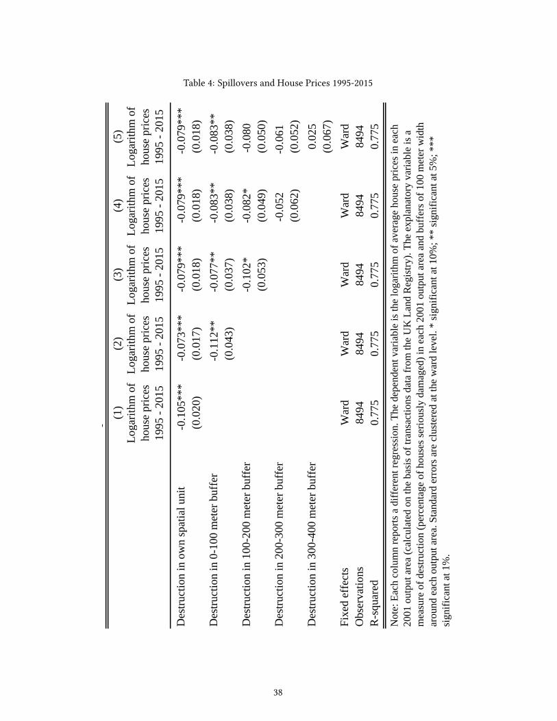
Table 4: Spillovers and House Prices 1995-2015

(1)

(2)

(3)

(4)

(5)

Loga

rithm

of

hous

e pr

ices

19

95 -

2015

Loga

rithm

of

hous

e pr

ices

19

95 -

2015

Loga

rithm

of

hous

e pr

ices

19

95 -

2015

Loga

rithm

of

hous

e pr

ices

19

95 -

2015

Loga

rithm

of

hous

e pr

ices

19

95 -

2015

Des

truct

ion

in o

wn

spat

ial u

nit

-0

.105

***

-0

.073

***

-0

.079

***

-0

.079

***

-0

.079

***

(0.0

20)

(0.0

17)

(0.0

18)

(0.0

18)

(0.0

18)

Des

truct

ion

in 0

-100

met

er b

uffe

r -

0.11

2**

-0.

077*

* -

0.08

3**

-0.

083*

*(0

.043

)(0

.037

)(0

.038

)(0

.038

)D

estru

ctio

n in

100

-200

met

er b

uffe

r-0

.102

*-0

.082

*-0

.080

(0

.053

)(0

.049

)(0

.050

)D

estru

ctio

n in

200

-300

met

er b

uffe

r-0

.052

-0

.061

(0

.062

)(0

.052

)D

estru

ctio

n in

300

-400

met

er b

uffe

r0.

025

(0.0

67)

Fixe

d ef

fect

sW

ard

War

dW

ard

War

dW

ard

Obs

erva

tions

8494

8494

8494

8494

8494

R-s

quar

ed0.

775

0.77

50.

775

0.77

50.

775

Tab

le 3

- Sp

illov

ers H

ouse

Pri

ces 1

995-

2015

Not

e: E

ach

colu

mn

repo

rts a

diff

eren

t reg

ress

ion.

The

dep

ende

nt v

aria

ble

is th

e lo

garit

hm o

f ave

rage

hou

se p

rices

in e

ach

2001

out

put a

rea

(cal

cula

ted

on th

e ba

sis o

f tra

nsac

tions

dat

a fr

om th

e U

K L

and

Reg

istry

). Th

e ex

plan

ator

y va

riabl

e is

a

mea

sure

of d

estru

ctio

n (p

erce

ntag

e of

hou

ses s

erio

usly

dam

aged

) in

each

200

1 ou

tput

are

a an

d bu

ffer

s of 1

00 m

eter

wid

th

arou

nd e

ach

outp

ut a

rea.

Sta

ndar

d er

rors

are

clu

ster

ed a

t the

war

d le

vel.

* si

gnifi

cant

at 1

0%; *

* si

gnifi

cant

at 5

%; *

**

sign

ifica

nt a

t 1%

.

38

Table 5: Social Composition of Neighbourhoods in 2001 Census

(1)

(2)

(3)

(4)

(5)

Inde

x of

so

cial

stat

usIn

dex

of

soci

al st

atus

Inde

x of

so

cial

stat

usIn

dex

of

soci

al st

atus

Inde

x of

so

cial

stat

us

Des

truct

ion

in o

wn

spat

ial u

nit

-14

.04*

** -

10.8

9***

-11

.46*

** -

11.4

3***

-11

.42*

**(1

.96)

(1.6

3)(1

.68)

(1.6

8)(1

.68)

Des

truct

ion

in 0

-100

met

er b

uffe

r -

11.0

5***

-8.

02**

-8.

40**

-8.

40**

(3.8

8)(3

.28)

(3.4

0)(3

.40)

Des

truct

ion

in 1

00-2

00 m

eter

buf

fer

-8.9

6*-7

.59*

-7.3

4*(4

.60)

(4.2

0)(4

.28)

Des

truct

ion

in 2

00-3

00 m

eter

buf

fer

-3.5

8 -4

.59

(5.4

0)(4

.77)

Des

truct

ion

in 3

00-4

00 m

eter

buf

fer

2.77

(5.8

0)Fi

xed

Effe

cts

War

dW

ard

War

dW

ard

War

dO

bser

vatio

ns86

2586

2586

2586

2586

25R

-squ

ared

0.47

30.

474

0.47

40.

474

0.47

4

Tab

le 4

- So

cial

Com

posi

tion

of N

eigh

bour

hood

s in

2001

Cen

sus

Not

e: E

ach

colu

mn

repo

rts th

e re

sults

of a

sepa

rate

regr

essi

on. T

he d

epen

dent

var

iabl

e is

a li

near

inde

x of

soci

al st

atus

for

each

200

1 ou

tput

are

a co

nstru

cted

usi

ng 2

001

cens

us d

ata

on o

ccup

atio

ns. S

ee th

e m

ain

text

for d

etai

ls. T

he e

xpla

nato

ry

varia

ble

is a

mea

sure

of d

estru

ctio

n (p

erce

ntag

e of

hou

ses s

erio

usly

dam

aged

) in

each

200

1 ou

tput

are

a an

d bu

ffer

s of 1

00

met

er w

idth

aro

und

each

out

put a

rea.

Sta

ndar

d er

rors

are

clu

ster

ed a

t the

war

d le

vel.

* si

gnifi

cant

at 1

0%; *

* si

gnifi

cant

at

5%; *

** si

gnifi

cant

at 1

%.

39

Table 6: Further Results on Mechanisms

(1)

(2)

(3)

(4)

(5)

(6)

(7)

(8)

Frac

tion

of

non-

whi

te

popu

latio

n

Frac

tion

of

non-

whi

te

popu

latio

n

Frac

tion

livin

g in

so

cial

ho

usin

g

Frac

tion

livin

g in

so

cial

ho

usin

g

Frac

tion

of

post

-war

ho

uses

Frac

tion

of

post

-war

ho

uses

Ave

rage

he

ight

of

build

ings

Ave

rage

he

ight

of

build

ings

Des

truct

ion

in o

wn

0

.075

***

0

.057

***

0

.153

***

0

.139

***

0

.295

***

0

.301

***

0

.773

***

0

.873

***

spat

ial u

nit

(0.0

11)

(0.0

10)

(0.0

21)

(0.0

17)

(0.0

24)

(0.0

23)

(0.2

91)

(0.3

15)

Des

truct

ion

in 0

-100

0.0

63**

*0.

041

-0.0

12

-0.5

08

met

er b

uffe

r(0

.019

)(0

.038

)(0

.044

)(0

.609

)D

estru

ctio

n in

100

-200

0.00

60.

049

-0.0

90

0.82

2m

eter

buf

fer

(0.0

24)

(0.0

43)

(0.0

57)

(1.0

20)

Des

truct

ion

in 2

00-3

00 0

.047

*-0

.020

0.

063

-0.5

72

met

er b

uffe

r(0

.026

)(0

.047

)(0

.060

)(0

.849

)D

estru

ctio

n in

300

-400

-0.0

11

-0.0

37

-0.1

31*

-0.9

10

met

er b

uffe

r(0

.028

)(0

.052

)(0

.068

)(1

.225

)Fi

xed

effe

cts

War

dW

ard

War

dW

ard

War

dW

ard

War

dW

ard

Obs

erva

tions

8625

8625

8625

8625

8625

8625

8625

8625

R-s

quar

ed0.

517

0.51

90.

371

0.37

20.

391

0.39

20.

319

0.32

0

Not

e: E

ach

colu

mn

repo

rts th

e re

sults

of a

sepa

rate

regr

essi

on. T

he d

epen

dent

var

iabl

e in

col

umns

(1) a

nd (2

) is t

he fr

actio

n of

peo

ple

in e

ach

2001

out

put a

rea

who

repo

rt th

eir e

thni

c ba

ckgr

ound

as n

on-w

hite

; in

colu

mns

(3) a

nd (4

) it i

s the

frac

tion

of p

eopl

e liv

ing

in

acco

mm

odat

ion

prov

ided

by

the

loca

l cou

ncil;

in c

olum

ns (5

) and

(6) i

t is t

he fr

actio

n of

201

4 ho

uses

that

did

not

exi

st w

ith th

e sa

me

foot

prin

t in

the

1930

s; in

col

umns

(7) a

nd (8

) it i

s the

ave

rage

hei

ght o

f bui

ldin

gs in

201

4 in

met

ers.

The

expl

anat

ory

varia

ble

is a

mea

sure

of

dest

ruct

ion

(per

cent

age

of h

ouse

s ser

ious

ly d

amag

ed) i

n ea

ch 2

001

outp

ut a

rea

and

buff

ers o

f 100

met

er w

idth

aro

und

each

out

put a

rea.

St

anda

rd e

rror

s are

clu

ster

ed a

t the

war

d le

vel.

* si

gnifi

cant

at 1

0%; *

* si

gnifi

cant

at 5

%; *

** si

gnifi

cant

at 1

%.

Tab

le 5

- Fu

rthe

r R

esul

ts o

n M

echa

nism

s

40