Estimating Information Cost Functions in Models of Rational

Inattention

Ambuj Dewan and Nathaniel Neligh∗

JOB MARKET PAPER

January 4, 2017

Abstract

In models of rational inattention, information costs are usually modeled using mutual infor-mation, which measures the expected reduction in entropy between prior and posterior beliefs,or ad hoc functional forms, but little is known about what form these costs take in reality. Weshow that under mild assumptions on information cost functions, including continuity and con-vexity, gross payoffs to decision makers are non-decreasing and continuous in potential rewards.We conduct laboratory experiments consisting of simple perceptual tasks with fine-grained vari-ation in the level of potential rewards that allow us to test several hypotheses about rationalinattention and compare various models of information costs via information criteria. We findthat most subjects exhibit monotonicity in performance with respect to potential rewards, andthere is mixed evidence on continuity and convexity of costs. Moreover, a significant portion ofsubjects are likelier to make small mistakes than large ones, contrary to the predictions of mu-tual information. This suggests that while people are generally rationally inattentive, their costfunctions may display non-convexities or discontinuities, or they may incorporate some notionof perceptual distance. The characteristics of a decision-maker’s information cost function haveimplications for various economic applications, including investment.

∗Ph.D. Candidates, Department of Economics, Columbia University. We are grateful to Mark Deanand Navin Kartik for their guidance on this project. We thank Marina Agranov, Jushan Bai, EthanBromberg-Martin, Alessandra Casella, Yeon-Koo Che, Judd Kessler, Jose Luis Montiel Olea, Pietro Or-toleva, Andrea Prat, Miikka Rokkanen, Christoph Rothe, Michael Woodford, and seminar and colloquiumparticipants at Columbia University for their helpful comments and suggestions. We would also like tothank the numerous colleagues who helped us test our experiments. We acknowledge the financial sup-port of grants from the Columbia Experimental Laboratory for the Social Sciences and the Microeco-nomic Theory Colloquium at Columbia University. The latest version of this paper can be found athttp://www.columbia.edu/∼ayd2105/jobmarketpaper.pdf.

1 Introduction

It has been observed in many settings that people have a limited capacity for attention, and this

affects the decisions they make. For example, Chetty et al. (2009) demonstrate that consumers

underreact to non-salient sales taxes; De los Santos et al. (2012) show that people only visit a

small number of online retailers before making book purchases; and Allcott and Taubinsky (2015)

provide evidence that people do not fully think about energy efficiency when making purchasing

decisions about light bulbs.1 Several laboratory experiments demonstrating limited attention have

been conducted, including Gabaix et al. (2006), Caplin and Martin (2013), and Caplin and Dean

(2014).

A common explanation for this phenomenon is the theory of rational inattention (Sims, 2003;

Sims, 2006; Caplin and Dean, 2015; Matejka and McKay, 2015). This theory posits that people ra-

tionally choose the information to which they attend, trading off the costs of paying more attention

with the ensuing benefits of better decisions. This decision-making process occurs in two stages. In

the first stage, the decision-maker chooses what information to acquire and pays costs accordingly.

In the second stage, the decision-maker uses the information she acquired to make decisions.

The first-stage information costs are typically assumed to have some fixed functional form.

Most common is mutual information (cf. Sims, 2003; Matejka and McKay, 2015), which measures

the expected reduction in entropy from a decision-maker’s prior beliefs to their posterior beliefs.

Other cost functions, such as fixed costs for information acquisition (e.g. Grossman and Stiglitz,

1980; Barlevy and Veronesi, 2000; Hellwig et al., 2012) or costs for increasing the precision of

normally distributed signals (e.g. Verrecchia, 1982; Van Nieuwerburgh and Veldkamp, 2010), have

also been used. However, little is known about what form these costs take in reality, and different

assumptions on these costs can lead to starkly different predictions.

In this paper, we use a laboratory experiment to characterize these information costs,2 a crucial

input for models of rational inattention. Subjects complete a series of perceptual tasks with fine-

grained variation in the levels of potential rewards. For each reward level, we observe both the

correct answer and the subject’s response. We interrogate these data in two ways: (1) testing various

properties of cost functions; (2) determining which models of information costs are consistent with

1For a survey that discusses many more similar field studies, see DellaVigna (2009).2We also conducted an online experiment, the results of which we report in Appendix C.

1

observed behavior.

The cost function properties of greatest interest to us are continuity, convexity, and perceptual

distance, the last of which refers to nearby states being harder to distinguish from each other than

distant ones. The presence or absence of each of these properties can have profound impacts on

the predictions of a model of rational inattention.

Continuity and convexity are important characteristics of many cost functions, such as the

aforementioned mutual-information cost function. The convexity of a cost function can greatly

affect model predictions. For example, Van Nieuwerburgh and Veldkamp (2010) study a portfolio

choice problem in which investors choose which assets to learn about and how much to learn

about each of them. Depending on the convexity of the investor’s utility and cost functions, it

can be optimal for the investor to learn about all available assets or to simply concentrate their

attention on a single asset; utility and cost functions that imply concave objective functions result

in generalized learning, whereas those that imply convex objective functions result in specialized

learning. Convexity also has implications for comparative statics in models of rational inattention.

As we prove in this paper, continuity and a specific form of convexity3 together imply that gross

payoffs (excluding information costs) change continuously in incentives.

Whether or not an information cost function embeds some notion of perceptual distance can

also have an effect on model predictions. Morris and Yang (2016) study a global game of regime

change where players acquire information at a cost. If nearby states of the world are sufficiently

costlier to distinguish from each other as compared to distant ones, then the game has a unique

equilibrium. This result stands in contrast to the result of Yang (2015), who studies a model where

information costs are such that nearby states are equally as easy to distinguish from each other as

distant ones and finds that the game has multiple equilibria.

In our experiment, we find that roughly one-third of the subjects whose performance on the tasks

improves with increasing potential rewards (whom we call “responsive subjects”) have behavior

that is consistent with “well-behaved” (i.e. continuous, convex) cost functions. Roughly 60% of

the responsive subjects have behavior consistent with a cost function that embeds some notion of

perceptual distance, in contrast to the mutual information cost function, which does not embed

such a notion.

3We call this form of convexity “almost strict convexity.” It is formally defined in Section 3.

2

The second important set of analyses in our paper fits various classes of cost functions to our

subjects’ data and selects the best fit for each subject. From subjects’ responses for each reward

level, we infer how their performance in the experimental tasks changes with potential rewards;

put differently, we estimate a performance function that traces out the relationship between the

potential reward and the probability of success. Each class of cost functions implies a specific

performance function, and so our model-fitting exercise involves determining which of these model-

implied performance functions most closely reflects each subject’s performance data.

Of particular interest to us are cost functions with fixed costs for information acquisition, normal

signals with linear precision costs, and the mutual information cost function, because of their usage

in the economic literature. The first implies a binary performance function with two levels of

performance, the second implies a concave performance function, and the third implies a logistic

performance function. Of the set of models we estimate, we find that the data of the subjects

who are responsive to incentives are best fit by one of these three models, with roughly a quarter

of subjects best fit by the first model, one-seventh of subjects best fit by the second model, and

two-thirds of subjects best fit by the third model. Thus, while there is some heterogeneity in the

population with respect to which cost functions best reflect human behavior, the set of potential

cost functions that we need to consider can be reduced to three cost functions commonly found in

the literature.

Finally, we apply the fixed-cost and mutual-information cost functions to a simple principal-

agent model of investment delegation and find that they imply starkly different comparative statics

results. Fixed costs for information acquisition imply payment structures that are discontinuous in

potential returns, whereas mutual information implies continuous payment structures.

To our knowledge, our paper is the first to use an experiment with fine-grained variation in

incentives to infer properties of information cost functions. This fine-grained variation is crucial

for testing the continuity and convexity of cost functions and for estimating subjects’ performance

functions, which is crucial for our model-fitting exercise. Although several papers have examined

competing hypotheses of dynamic evidence accumulation using perceptual data,4 ours is the first

to run a “horse race” between a large number of types of cost functions in a static model of rational

inattention.

4We discuss some of this literature in the following section.

3

The remainder of the paper proceeds as follows. Section 2 reviews various experimental ap-

proaches to limited attention in the literature. Section 3 presents the theoretical framework that we

use in this paper. Section 4 introduces the type of task that we implement in our experiment and

situates it within our theoretical framework. Section 5 introduces various models of cost functions

and applies them to the tasks of our experiment. Section 6 presents our experimental design and

compares it to previous experiments about limited attention. Section 7 presents and discusses basic

experimental results and categorizes subjects according to the behaviors they exhibit. Section 8 fits

various models of cost functions to the subjects’ data and runs a “horse race” to determine which

is the best fit for each subject. Section 9 presents additional results relating to demographics and

reaction times. Section 10 presents an application of our results to the delegation of investment.

Section 11 concludes. Most proofs are relegated to Appendix A. Additional experimental results

are reported in Appendices B and C.

2 Related Literature

One approach that has been taken in the experimental literature to examine limited attention has

been to give subjects a series of perceptual and/or cognitive tasks and observe their responses.

Several experiments use this technique to test implications and fit parameters of models of limited

attention. Caplin and Dean (2014) use a task involving the counting of differently-colored balls to

test the necessary and sufficient conditions for a model of rational inattention with discrete choices

where information acquisition is modeled as a static process. Caplin and Dean (2013) use that same

task to estimate subjects’ cost parameters in a mutual information cost function. Shaw and Shaw

(1977) employ a protocol where stimuli are presented at random locations on a tachistoscope.5

Using the data they obtained, they estimate how much attention the subjects allocated to those

locations on their visual field. Gabaix et al. (2006) use an experiment involving the comparison of

multiattribute choices to calibrate a model of myopic search.

This parameter-fitting approach has also been extended outside of the domain of visual per-

ception to the domain of relative value assessment. Krajbich et al. (2010) ask subjects to choose

between pairs of snack food items that the subjects have rated on a numerical preference scale,

5A tachistoscope is a device used to present visual stimuli for a controlled duration. It has become much lesscommon in behavioral research since the advent of personal computers.

4

and using choice and reaction-time data, they estimate the parameters of a drift-diffusion model

(DDM), where information acquisition is modeled as a dynamic process.

There is a large literature that uses choice and reaction-time data to compare models of evidence

accumulation. For example, Woodford (2014) presents a model of dynamic evidence accumulation

with mutual-information costs and uses Krajbich et al.’s data to compare the fit of his optimizing

model to the DDM, and Ratcliff and Smith (2004) use data from several experiments to compare

the fits of four different dynamic evidence accumulation models.

Our experiment synthesizes these approaches. Using choice data from an experiment with

perceptual tasks, we test hypotheses about behavior, including necessary and sufficient conditions

for rational inattention, convexity and continuity of cost functions, and whether subjects are better

at distinguishing nearby states from distant ones. We also estimate parameters of various models

of rational inattention and then compare their fits to each other.

The tasks in our experiment involve the perception of numerosity, a long-standing area of

research in perceptual psychology. Our tasks are similar to those implemented by Saltzman and

Garner (1948) and Kaufman et al. (1949), who present subjects with fields of randomly arranged

dots whose numerosity they have to judge. More recently, the ball-counting tasks of Caplin and

Dean (2014) have also involved the perception of numerosity.

3 Theoretical Framework

Various models of limited attention and imperfect perception have been proposed in the literature.

These models can be classified along two axes: optimizing vs. non-optimizing; and static vs.

dynamic.

In optimizing models, the information acquired by a decision-maker depends on an explicit

choice that is made optimally given their cost and/or constraints. As a result, any “errors” observed

in their decisions can be considered rational. By contrast, in non-optimizing models, errors in

decisions or perception are the result of some exogenous process that is not chosen by the decision-

maker; the choice of information is not explicitly modeled or is assumed to be out of the decision-

maker’s control.

Models of limited attention and imperfect perception can also be classified according to whether

5

they are static or dynamic. In static models, information acquisition is modeled as a one-time

occurrence; either the decision-maker makes a single information-acqusition choice, or information

is modeled as if it is delivered to the decision-maker all at once. On the other hand, in dynamic

models, information is accumulated over time. That is not to say that static models cannot be

applied to situations where information acquisition is a dynamic process; static models simply

restrict their scope to the outcome of such a process, not the process itself.

We refer to the class of optimizing models as models of rational inattention. In particular, this

paper considers a general static model of rational inattention with finite state and action spaces

and additively separable costs. Such a model is the focus of Caplin and Dean (2015) (henceforth

CD15), who derive necessary and sufficient conditions for observed behavior to be consistent with

it. Other papers have considered static rational inattention models with specific cost functions.

For example, Matejka and McKay (2015) derive the implications of the mutual-information cost

function, and Woodford (2012) considers the prior-independent channel-capacity cost function.

There are also several static, non-optimizing models of limited attention and imperfect per-

ception. In consumer choice, one class of papers studies the imperfect perception of attributes

of multi-attribute choices and introduces distortions to those attributes that depend on the set

of available choices (e.g. Bordalo et al., 2013; Koszegi and Szeidl, 2013; Bushong et al., 2014).

These distortions are exogenously imposed; they are not chosen by the decision-maker. The size

and extent of these distortions can be seen as a measure of the consumer’s inattention. In per-

ceptual psychology, signal detection theory (cf. Chapter 12 of Frisby and Stone, 2010) provides

an important theoretical framework for studying imperfect perception. In this framework, states

of the world are observed with exogenously given noise, and the decision-maker must determine

what the most likely state was given their observations. We implement a task of this nature in our

experiment; however, we model the noise process as an endogenous choice.

Dynamic models of evidence accumulation have a long tradition in mathematical psychology.

In drift-diffusion models (DDMs) (e.g. Ratcliff, 1978; Diederich, 1997), evidence is modeled as a

stochastic process that evolves according to a diffusion process (Smith, 2000), such as Brownian

motion. The decision-maker stops gathering evidence and makes a decision when this process

hits some (possibly time-dependent) boundary. This boundary is often exogenously given, as in

Ratcliff (1978), implying a non-optimizing modeling approach. However, under some conditions, the

6

boundary can be derived as the result of an optimal stopping problem (e.g. Fudenberg et al., 2015;

Tajima et al., 2016). Other optimizing approaches consider the optimal selection of the intensity

of evidence accumulation when the stopping rule is exogenously given (e.g. Woodford, 2014) or

the optimal selection of both evidence accumulation intensity and stopping rule (e.g. Moscarini

and Smith, 2001). The vast majority of these dynamic evidence accumulation models restrict their

focus to situations where the decision-maker must choose between two options, though Moscarini

and Smith extend their model to consider situations with multiple discrete choice alternatives.

In this paper, we adopt a static framework that allows us to consider any finite number of

options for the decision-maker as well as a flexible choice of information-acquisition technologies.

3.1 General Model

In remainder of this section, we present a general framework for analyzing problems of rational

inattention. In this framework, there is an unknown state of the world about which an decision-

maker (DM) can choose to acquire information. This information affects her beliefs about the state

of the world. After obtaining this information, she makes a decision that maximizes her payoff

given her beliefs.

We model information as a collection of probabilistic mappings from states of the world to a set

of subjective signals. We define an information structure to be a set of conditional distributions

of signals given states. Observing a signal generates a corresponding posterior belief over states.

Given this posterior belief, the DM maximizes her payoff by guessing the most likely state. Each

information structure has a cost associated with it.

We remain agnostic about what the exact source of information costs is. Information costs

could represent cognitive or physical effort exerted in learning about the true state, as well as the

opportunity cost of time spent doing so.

This framework has several beneficial features. Firstly, it has the same behavioral implications

as the model of CD15, which means we can apply their necessary and sufficient conditions for models

of rational inattention to the problems we study. Secondly, it expresses information structures as

stochastic matrices, which as demonstrated later in the paper, will permit us to easily compare

information structures and to define a simple geometric notion of convexity of information costs.

7

Let Θ = {θi}|Θ|i=1 be a finite state space, let M = {mi}|M |i=1 be a finite signal space,6 and let

A = {ai}|A|i=1 be a finite action space, with |M | ≥ |A| so that there are at least as many signals

as there are actions. Let π = (πi)ni=1 ∈ ∆(Θ), where n := |Θ|, be the DM’s prior over Θ. Each

action-state pair (a, θ) has an associated utility u(a, θ). The DM maximizes:

EγQ[E〈π|m〉 [u(a, θ)]

]− C(π,Q) (1)

where Q is an information structure (a collection of conditional signal probabilities, given states),

γQ is the distribution of posterior beliefs it induces, and 〈π|m〉 is the posterior belief associated

with signal m.

As explained above, the DM’s problem has two stages. First, she selects an information structure

Q. She then observes a signal m according to that information structure, which gives her a posterior

belief 〈π|m〉. Second, given this posterior belief, she chooses an action a to maximize her expected

payoff.

We can express this problem more formally using matrix notation. Let Π = diag(π).7 Let

U ∈M|A|×|Θ|(R) be a matrix with entries ui,j := u(ai, θj), i.e. the utility of taking action i in state

j. We refer to U as the payoff matrix.

Let Q be the space of right-stochastic matrices of dimension |Θ| × |M |, and let D be the space

of right-stochastic matrices of dimension |M |×|A|. C : ∆(Θ)×Q −→ R gives the cost8 of selecting

an information structure from Q, given a prior in ∆(Θ).9

6 Given that the state space is finite, the finiteness of the signal space is not a substantive restriction. In fact, ifwe assume that more informative information structures are costlier (our Restriction E, presented later in the paper),it can be shown that given a finite state space, a DM never need use more than a finite number of signals. Thisfollows from Proposition 4 of Kamenica and Gentzkow (2010). They study a game where the information structureand the action are chosen by different players, but if we assume those players’ preferences are perfectly aligned, thenignoring information costs, our framework maps onto theirs. By their Proposition 4, if a DM employs an informationstructure with an infinite number of signals, then ignoring information costs, she could have done at least as wellwith an information structure with a finite number of signals. Moreover, since the former information structure ismore informative than the latter, it is costlier. Therefore, the DM will choose to use a finite number of signals.

7diag(x) is the square matrix that has the entries of x in order on its diagonal and zeroes elsewhere.8 R := R ∪ {−∞,∞} is the set of extended reals. If for some π and Q, C(π, Q) = ∞, then the cost of the

information structure Q given π is infinite, and the DM will never select it, provided there is at least one informationstructure available at a finite cost.

9In principle, though the cost-function approach implies flexibility in the selection of information structures, itcan accommodate restrictions on the space of available information structures as well. For example, if Q is the setof admissible structures, then C(π,Q) is finite if Q ∈ Q and infinite otherwise. If a modeler wishes to impose anexogenous process of information acquisition, then he may simply set Q to be a singleton.

8

The decision-maker’s problem, then, is (cf. Leshno and Spector, 1992):10

maxQ∈Q,D∈D

tr(QDUΠ)− C(π,Q) (2)

where the entries of Q are qi,j = Pr(mj |θi), i.e. the probably of signal mj in state θi, and the

entries of D are di,j = Pr(aj |mi), i.e. the probability of selecting action aj given signal mi. We

denote the distribution of posteriors (with finite support) that Q induces by γQ ∈ ∆(∆(Θ)). The

i-th row of Q represents the conditional distribution of signals given state θi, and so Q can be seen

as a collection of signal distributions given states. We refer to D as the decision matrix.

We refer to the maximand in (2) as the net payoff and its first component as the ex-ante gross

payoff. Specific realizations of this payoff are called the ex-post gross payoff. Where it will not

cause confusion, we will drop the “ex-ante” and “ex-post.”

This setup allows us to index decision problems of the form of (2) by (π, U). In this paper,

we will hold π fixed, and thus we will simply index decision problems by U where it will cause no

confusion. If we give a DM a finite set of decision problems {Ui}, then we can observe the true

state θi chosen by nature and action ai chosen by the DM for each decision problem. Using the

data set {(Ui, θi, ai)} will allow us to infer the properties of C(·, ·). We refer to a data set of this

type as stochastic choice data.

At this point, it may be useful to consider a rewritten version of (2):

maxQ∈Q,D∈D

n∑i=1

πi

|A|∑j=1

uj,i

|M |∑k=1

qi,kdk,j

− C(π,Q) (3)

This version of the DM’s problem allows us to see how the ex-ante gross payoff is constructed. For

each (i, j),|M |∑k=1

qi,kdk,j = Pr(aj |θi) is the probability of taking action j in state i. Summing these

probabilities and weighting by the utilities for each action gives|A|∑j=1

uj,i

[|M |∑k=1

qi,kdk,j

], the expected

utility in state i, given the subject’s choice of information structure and decision matrix. Summing

these expected utilities and weighting by the probability of each state gives the total ex-ante gross

payoff,n∑i=1

πi

[|A|∑j=1

uj,i

[|M |∑k=1

qi,kdk,j

]].

In this setup, for each i ∈ {1, . . . , n} and j ∈ {1, . . . , |A|}, πi and uj,i, are exogenous parameters.

10tr(X) denotes the trace of X, the sum of its diagonal entries.

9

For each i ∈ {1, . . . , n}, j ∈ {1, . . . , |A|}, and k ∈ {1, . . . , |M |}, qi,k and dk,j are chosen by subjects.

Though one cannot observe qi,k and dk,j separately, one can observe the products qi,kdk,j , i.e. if a

DM solves the same decision problem repeatedly, one can observe how often each action is chosen

in each state.

3.2 Cost Equivalence

As written, the model Subsection 3.1 generalizes the model of rational inattention studied by

CD15, assuming a finite set of actions. In contrast to their model, our model allows for the cost

of a distribution of posteriors to depend on the specific signals that generated each posterior in its

support. Put differently, a version of their model with a finite number of actions is equivalent to

ours with the following restriction.

Restriction A. Cost equivalence. For all priors π, C(π,Q1) = C(π,Q2) whenever Q1 and Q2

induce the same distribution of posteriors.

However, as we show below, cost equivalence imposes no additional behavioral restrictions,

and therefore, any behavior that is consistent with our model is also consistent with CD15. This

result allows us to apply CD15’s necessary and sufficient conditions for rational inattention to our

framework without imposing any restrictions.

Proposition 1. Stochastic choice data are consistent with (2) iff they are consistent with CD15.11

To outline the proof, the ‘if’ direction is obvious, since our model generalizes CD15. To see the

‘only if’ direction, suppose that {(Ui, θi, ai)} can be rationalized by (2) with some cost function

C(π,Q). Define QγQ to be set of information structures that induce the distribution γQ over

posteriors, and define C(π,Q) := minR∈QγQ

C(π,R). It is obvious that C satisfies cost equivalence.

Moreover, since a given posterior distribution always induces the same ex-ante gross payoff, the

DM should always choose the lowest-cost way of inducing that posterior distribution. Thus, the

proof boils down to showing that this minimum is well-defined. Details are in Appendix A.

11Though we have a assumed a finite action space in our paper, the proof of Proposition 1 does not rely on this.

10

3.3 Testing for Rational Inattention

As CD15 demonstrate, observed behavior is consistent with their model if and only if it satisfies their

“no improving attention cycles” (NIAC) and “no improving action switches” (NIAS) conditions.

Their NIAC condition ensures that improvements to gross payoffs cannot be made by reallocating

attention cyclically across decision problems, and their NIAS condition ensures that the DM’s

actions are optimal given the beliefs induced by her chosen information structure. Because our

model is behaviorally equivalent to theirs, NIAC and NIAS are necessary and sufficient conditions

for stochastic choice data to satisfy our model. Put differently, the DM fails to fulfill either of those

two conditions if and only if there does not exist a cost function that rationalizes her stochastic

choice data.

In our notation, the NIAC condition can be expressed as follows. Assume a fixed prior π,

and let U0, U1, . . . , UJ−1 be any set of two or more payoff matrices. Let Q0, Q‘, . . . , QJ−1 and

D0, D1, . . . , DJ−1 be the corresponding information structures and decision matrices selected by

the DM, and let Dji be a decision matrix that maximizes the gross payoff given payoff matrix Ui

and information structure Qj . Then the NIAC condition states:

J−1∑j=0

tr (QjDjUjΠ) ≥J−1∑j=0

tr(Q(j+1) mod JD

(j+1) mod Jj UjΠ

)(4)

The NIAS condition can be expressed as follows. Assume a fixed prior π. Then for any payoff

matrix U , let Q∗ be the information structure and D∗ be the decision matrix chosen by the DM.

Then the NIAS condition states that for any k ∈ {1, . . . , |A|} such that the k-th column of D∗

(denoted by d∗•,k) has at least one nonzero entry and any l ∈ {1, . . . , |A|}:

uk,•ΠQ∗d∗•,k ≥ ul,•ΠQ∗d∗•,k (5)

where uk,• and ul,• are the k-th and l-th rows of U , respectively.

Proposition 2. NIAC and NIAS are necessary and sufficient conditions for stochastic choice data

to satisfy (2).

Proof. This follows directly from Proposition 1 of the present paper and Theorem 1 of CD15.

11

3.4 Responsiveness

A set of behaviors that is consistent with rational inattention is one where the DM’s behavior

does not change across decision problems; regardless of the decision problem, she chooses the same

information structure and decision matrix. This is consistent with models such as signal detection

theory, where the DM’s information structure is exogenously given. In those cases, the DM simply

does not respond to changes in incentives across decision problems. More interesting are cases

where the DM does modify her behavior in response to changes in incentives.

Definition 1. Suppose that a DM is given a set of decision problems U = {U1, U2, . . . UJ}. Further

suppose that ∃U, U ∈ U satisfying the following: for each i ∈ {1, . . . n}, let τi ∈ argmaxj∈{1,...,|A|}

ui,j ;

∀ i ∈ {1, . . . n}, ui,j ≥ ui,j if j = τi and ui,j ≤ ui,j if j 6= τi, with at least one strict inequality. Then

we say the DM is responsive (to incentives) (or exhibits responsiveness) if her behavior is such that

Pr

(a ∈ argmax

z∈A∈ u(z, θ)

)> Pr

(a ∈ argmax

z∈A∈ u(z, θ)

).

Put differently, a DM is responsive to incentives if for some pair of decision problems, her

probability of taking a (gross) payoff-maximizing action increases when the utility associated with

payoff-maximizing actions increases and the utility associated with non-payoff-maximizing actions

decreases.

Responsiveness is a fairly intuitive condition for human behavior to fulfill. Roughly speaking,

it says that people perform better (by choosing the best option more often) when the stakes are

higher.

3.5 Continuity and Convexity

In this subsection, we establish sufficient conditions for continuous gross payoffs in general rational

inattention problems. Roughly speaking, continuity and convexity of the information cost function

imply gross payoffs that are continuous in incentives.

Restriction B. Continuity. C(π,Q) is continuous in its second argument.12

Continuity is a typical assumption in much of economic analysis. In this case, it implies that

gathering a small amount of additional information increases the total cost of information by only

12Because R is not metrizable with the standard Euclidean topology, we are implicitly assuming here that C mapsto R, i.e. it is nowhere infinite.

12

a small amount. This may seem like a fairly innocuous assumption, but it precludes some plausible

cost functions, such as those with fixed costs for information acquisition, as will be seen in Section

5.

Restriction C. Convexity. ∀π ∈ ∆(Θ), ∀λ ∈ (0, 1), ∀Q1, Q2 ∈ Q, C(π, λQ1 + (1 − λ)Q2) ≤

λC(π,Q1) + (1− λ)C(π,Q2).

Restriction D. Almost strict convexity. ∀π ∈ ∆(Θ), ∀λ ∈ (0, 1), ∀Q1, Q2 ∈ Q, C(π, λQ1 +

(1− λ)Q2) ≤ λC(π,Q1) + (1− λ)C(π,Q2), where the inequality is strict except possibly if Q1 and

Q2 induce the same distribution of posteriors.

These notions of convexity can be contrasted with CD15’s. CD15 define a notion of convexity

over the space of distribution of posteriors called “mixture feasibility”;13 however it is not testable.

In our framework, cost functions are defined over stochastic matrices instead of the distributions

of posteriors they induce. Since the space of stochastic matrices can be identified with a subset of

Euclidean space, Restrictions C and D give us easily interpretable “geometric” notions of convexity.

Moreover, Restriction D has testable implications.

It is clear that Restriction D is a special case of Restriction C. Restriction D is also a slight

relaxation of strict convexity. We employ this slight relaxation because strict convexity would be

incompatible with Restriction A, cost equivalence. To see why, consider the 2× 2 case where Q1 = 0.25 0.75

0.25 0.75

, Q2 =

0.75 0.25

0.75 0.25

, and Q3 = 0.5Q1 + 0.5Q2 =

0.5 0.5

0.5 0.5

. In all three

of these information structures, a given signal is induced by each state with the same probability.

Therefore, the distribution of posteriors each one generates is the degenerate distribution on the

prior, and by cost equivalence, all three information structures should have the same cost. However,

Q3 is a convex combination of Q1 and Q2, and so if the cost function were strictly convex it would

have to have a strictly lower cost than Q1 or Q2. Thus, Restriction A is incompatible with strict

convexity. However, under almost strict convexity, Q3 would be permitted to have the same cost

as Q1 and Q2.

In order to ensure that continuity and almost strict convexity imply continuous gross payoffs,

we require two additional conditions.

13Restriction C involves mixtures of conditional signal probabilities, which could yield posteriors not generated byeither information structure in the mixture, whereas mixture feasibility involves mixtures of distributions of posteriorswhose support is the union of the supports of the distributions in the mixture.

13

Restriction E. Monotonicity of information. Let R be a right-stochastic matrix of dimension

|M |× |M |, which we refer to as a garbling matrix. Then for any π ∈ ∆(Θ) and Q ∈ Q, C(π,Q) ≥

C(π,QR).

Restriction E is equivalent to Condition K1 of CD15. If Q is an information structure and

R is a garbling matrix, then Q can be thought of as containing all the information contained in

QR, i.e. QR simply adds noise to Q. In this case, we shall say that Q Blackwell-dominates QR.

As shown by Blackwell (1953), Q yields a (weakly) higher gross payoff than QR for any decision

problem, given an optimal selection of decision matrices. Therefore, Restriction E implies that if

one information structure is more informative than another, then it is also costlier. This restriction

does not provide a complete order on information costs, since it is possible that two experiments are

not ranked in the Blackwell sense. In other words, if Q1 and Q2 are information structures of the

same dimension, there does not necessarily exist R of appropriate dimension such that Q1R = Q2

or Q2R = Q1.

CD15 show that this restriction is not testable; any stochastic choice data set that is consistent

with some cost function C is also consistent with some cost function C that satisfies Restriction E.

Therefore, requiring it does not eliminate any additional sets of stochastic choice data from being

consistent with a model of rational inattention.

Restriction F. Cost symmetry. Let R be a |M |×|M | permutation matrix. Then ∀Q ∈

Q, C(π,Q) = C(π,QR).

It is easy to see that cost equivalence (Restriction A) implies cost symmetry. This restriction

says that the cost of an information structure is invariant to the labeling of its signals; only the

conditional probabilities of generating each signal matter.

We have now established a set of sufficient conditions that ensure that the DM’s ex-ante gross

payoff is continuous in incentives.

Proposition 3. Suppose that π is fixed and C satisfies Restrictions B, D, E, and F. Then the

ex-ante gross payoff is continuous in U .

Monotonicity of information and cost symmetry ensure that the decision matrix chosen by the

DM can be fixed, which in turn ensures the convexity of the problem. While almost strict convexity

14

does not ensure a unique solution to the problem, it does ensure that the optimal ex-ante gross

payoff is single-valued, which together with the continuity of the cost function implies the result.

At this point, a clarification is in order. Proposition 3 is a statement about what the properties

of an information cost function imply about behavior. To obtain a statement about what behavior

implies about the properties of cost functions, we invoke the contrapositive: if gross payoffs are

discontinuous in incentives, then this behavior cannot be rationalized by an information cost func-

tion that satisfies Restrictions B, D, E, and F simultaneously. However, as we explained earlier in

this subsection, Restrition E is not testable, and furthermore, since Restriction F is implied by the

untestable cost-equivalence Restriction A, it is also untestable. Therefore, given stochastic choice

data, we can assume the cost function that rationalizes it satisfies Restrictions E and F, and so if

we observe that ex-ante gross payoffs are discontinuous in incentives,14 then this implies that the

DM’s cost function either is discontinuous or fails almost strict convexity.

The restrictions necessary for 3 are satisfied by many different cost functions. In particular,

cost functions that can be expressed as a sum of convex functions of the entries of a stochastic

matrix are almost strictly convex.

Proposition 4. Let {ci,j(·, ·)}, i ∈ {1, . . . , n}, j ∈ {1, . . . , |M |} be a collection of continuous

functions on ∆(Θ) × [0, 1] such that for fixed π, each ci,j(π, ·) is a twice continuously differen-

tiable function with R with∂2ci,j(π,·)

∂q2> 0 ∀ q ∈ (0, 1), ∀ i ∈ {1, . . . , n}, ∀ j ∈ {1, . . . , |M |}. Then

C(π,Q) :=∑

i,j ci,j(π, qi,j) satisfies Restrictions B through D.

4 Uniform Guess Tasks

Consider a task where there is some unknown true state of the world that a decision-maker (DM)

has to identify, and learning about the true state is costly. There are n possible states, each of which

is a priori equally likely. The DM receives a reward r for correctly identifying the state and no

reward for incorrectly identifying the state. Therefore, the DM’s goal is to maximize her probability

of correctly identifying the state, net of whatever costs she incurs in gathering information about

the true state. We refer to tasks with this setup as uniform guess tasks.

14The reader may have noticed that strictly speaking, observing a discontinuity is technically impossible withoutan infinite data set. We expound upon this point in the following section. For now, simply assume that the datastrongly suggest that gross payoffs are discontinuous in incentives.

15

An example of such a task is the type of task we implement in our experiment. In this type of

task, which we refer to as the “dots” task, the DM is shown a screen with a random arrangement

of dots. Her goal is to determine the number of dots on the screen, which is between 38 and 42,

inclusive, with each possible number equally likely. She receives a reward r for correctly guessing

the number of dots and no reward otherwise.

In our example, information costs could include the cost of effort exerted in counting dots,

cognitive costs incurred in employing an estimation heuristic, or the opportunity cost of time spent

trying to determine the number of dots.

In a uniform guess task, the DM’s goal is to choose an information structure to maximize:

r

n

∑x

Pr(a = x|θ = x)− C(πunif, Q) (6)

where θ is a state of the world, a is the subject’s guess of the state, and C(πunif, Q) is the cost

associated with information structure Q and the uniform prior. Put differently, the DM rationally

chooses an information structure to maximize her net payoff (6). Thus, uniform guess tasks can be

considered problems of rational inattention. The cost function C(πunif, Q) is the primary object of

interest in our experiment.

4.1 Applying the General Model and Performance Functions

The general model we presented in Section 3 can be applied to uniform guess tasks. In these decision

problems, since the DM is trying to determine the true state, we can set A = Θ. Moreover, U = rIn

for some r > 0. Therefore, the DM’s ex-ante gross payoff in this task can be written as rtr(QDΠ).

Note that P := tr(QDΠ) = 1ntr(QD) is the ex-ante probability of correctly guessing the state,

which we call their performance. For each reward r, the DM’s optimal choice of Q and D induce an

optimal performance P ∗(r), which we call the performance function. We can estimate P ∗(r) from

stochastic choice data, and by studying its properties, we can infer the properties of the DM’s cost

function.

Given some choice of Q, the DM should optimally choose D so that given a signal, she chooses

the most likely state; put differently, she should choose the matrix D that selects the maximal

16

element in each column of Q. Thus, if the DM’s choice of D is optimal, then:

P ∗(r) =1

n

|M |∑j=1

maxi∈{1,...,n}

qi,j (7)

4.2 Rational Inattention

In uniform guess tasks, NIAC can be tested by looking at the performance function P ∗(r).

Proposition 5. In a set of uniform guess tasks, the DM’s behavior is consistent with NIAC iff

P ∗(r) is nondecreasing.

In other words, the DM’s behavior is consistent with NIAC if and only if she performs no worse

when given higher incentives; she allocates her attention such that she pays more attention to more

valuable tasks.

For testing NIAS in uniform guess tasks, we require a more detailed summary of the data than

the performance function; simply looking at which questions were answered correctly or incorrectly

is insufficient.

Proposition 6. In a set of uniform guess tasks, the DM’s behavior is consistent with NIAS iff

∀x ∈ A, ∀ y ∈ Θ,Pr(θ = x|a = x) ≥ Pr(θ = y|a = x).

In other words, the DM’s behavior is consistent with NIAS if and only if the mode of each

posterior distribution of states given an action is equal to that action; if an outside observer were

to see the DM’s actions without observing the true states, then his best guess of the true state for

any task would be the answer given by the DM.

4.3 Responsiveness

In a set of uniform guess tasks, any pair of tasks with different reward levels satisfies the conditions

required for the definition of responsiveness. This is easy to see: the utilities associated with payoff-

maximizing actions are constant within each corresponding payoff matrix and higher in one payoff

matrix than the other. Furthermore, the utilities associated with non-payoff-maximizing actions

are all zero. Therefore, responsiveness in uniform guess tasks boils down to there being at least

one pair of reward levels such that the DM performs strictly better at the higher reward level than

at the lower one.

17

Thus, responsiveness implies that the performance function cannot be flat everywhere. In other

words, it must have a region of strict increase.

4.4 Continuity and Convexity

In uniform guess tasks, Proposition 3 has a simple implication for behavior: if the conditions of the

proposition are satisified, then performance is continuous in reward.

Proposition 7. If C satisfies Restrictions B, D, E, and F, then P ∗(r) is continuous.

Proof. Since optimal gross payoffs are given by rP ∗(r), this follows immediately from Proposition

3.

Using the same contrapositive reasoning as we did in Subsection 3.5, this means that if we

observe a discontinuous performance function, then the DM’s cost function either is discontinuous

or violates almost strict convexity.

4.5 Perceptual Distance

In uniform guess tasks, where the action space is identified with the state space, we can establish

a meaningful concept of perceptual distance. Perceptual distance refers to the notion that distant

states are easier to distinguish from each other than nearby ones. For example, if Θ = {1, 2, 3, 4, 5},

and the true state is θ = 2, then the DM may be more likely to answer 1 (which is 1 away from

2) than she is to answer 5 (which is 3 away from 2). This is especially plausible if the states in

Θ represent physical, measurable quantities. To give a more concrete example, when shopping for

televisions, one is much more likely to misperceive a 27-inch screen as a 23-inch screen than as a

40-inch screen. We formalize this notion below.

Definition 2. Let ρ be a metric on Θ. Then in this task, the DM evinces the perception of distance

iff ∀x, y, z ∈ Θ, ρ(x, y) > ρ(x, z) =⇒ Pr(a = y|θ = x) < Pr(a = z|θ = x).

In other words, the DM evinces the perception of distance if for each possible true state, she is

more likely to give an answer close to the true state than one farther away from it.

Though one can define a metric on a given set in many different ways, it makes sense to take ρ

to be a “natural” metric on Θ. For instance, if Θ is a subset of the real line as in the example above,

18

then absolute value, ρ(x, y) = |x − y|, may be a sensible metric to use. Since the state space in

our experiment is such a subset, absolute value is the metric we use in analyzing our experimental

results.

5 Cost Functions

The space of admissible cost functions is vast. Indeed, any cost function C : ∆(Θ)×Q −→ R leads

to behavior consistent with NIAS and NIAC. In this subsection, we introduce the classes of cost

functions that are most relevant for our analysis and derive their behavioral implications.

5.1 Mutual Information

Mutual information is one of the most common information cost functions in the economic literature,

having been used since at least Sims (2003). Mutual information is defined as the expected reduction

in entropy from the prior to the posterior. If we denote the mutual information cost function by I

and entropy by H, then:

I(π,Q) := α(H(π)− E[H(π|Q)]) = α

− n∑i=1

πi lnπi −

− n∑i=1

πi

|M |∑j=1

qi,j ln

(πiqi,j∑nk=1 pkqk,j

)(8)

where α > 0 and we adopt the convention that 0 ln 0 = 0 and 0 ln 00 = 0.

Mutual information satisfies some of the restrictions of Section 3.

Proposition 8. Mutual information satisfies Restrictions A, C, E, and F.

In uniform guess tasks, we can derive closed-form expressions for the DM’s optimal behavior.

Proposition 9. Suppose that πi = 1n ∀i ∈ {1, . . . , n} so that the prior is uniform on Θ and that

C(π,Q) = I(π,Q) := α(H(p)−E[H(π|Q)]), α > 0, i.e. C is the mutual information cost function.

Then, the probability of guessing the correct state is continuous in the reward. Moreover, this

probability is given by P ∗(r) =exp( rα)

n−1+exp( rα), and the probability of guessing any given incorrect state

is 1n−1+exp( rα)

.

Proof. This follows directly from Proposition 1 of Matejka and McKay (2015).

19

Note that mutual information is convex, but it can be shown that it is not almost strictly

convex, i.e. it does not satisfy Restriction D.15 Therefore, Proposition 9 cannot be derived as a

special case of Proposition 3.

There are two important things to note about Proposition 9. The first is that mutual information

implies a logistic performance function, which is defined by a single parameter α. The second is

that for any given true state θ, the probability of answering each incorrect state is equally likely,

i.e. a DM with a mutual information cost function does not evince the perception of distance.

5.2 Fixed Costs

Another common model of information costs in the literature is “all-or-nothing” costs, where the

DM begins with no information but can become completely informed about the state of the world

if she pays a cost (e.g. Grossman and Stiglitz, 1980; Hellwig et al., 2012). Here, we generalize this

form of costs by allowing for the DM to receive some information for free and pay a fixed cost to

receive more information; we do not stipulate that she must become fully informed.

We can represent this situation as follows. Let there exist Q, Q such that Q = QR for some

garbling matrix R (so that Q is more informative than Q in the Blackwell sense) and:

C(Q) =

0, Q = Q

κ, Q = Q

∞, otherwise

(9)

According to this cost function, the DM can receive the information contained in Q for free, but

she must pay a fixed cost κ to acquire the information in Q.

Cost functions with fixed costs such as these can be seen as representing dual-system cognitive

processes (cf. Stanovich and West, 2000; Kahneman, 2003). In such processes, a small amount

of information may be acquired at a very low cost, but there is a fixed cost to acquiring more

information. This implies a discontinuity in the cost function between information structures with

15 For example, let Q1 =

14

116

18

916

14

18

316

716

14

316

14

516

14

14

116

716

and Q2 =

18

796

748

2132

18

748

732

4996

18

732

724

3596

18

724

796

4996

. These two information struc-

tures induce different distributions of posteriors (albeit with the same support). However, it can be shown that anyconvex combination Qλ := λQ1 + (1 − λ)Q2, λ ∈ [0, 1] of them is such that I(π,Qλ) = λI(π,Q1 + (1 − λ)I(π,Q2),thereby violating almost strict convexity.

20

Figure 1: Fixed cost for information acquisition. The left panel shows the cost function, and theright panel shows the resulting performance curve. Parameters are κ = 30, q = 0.3, and q = 0.8.

“low” informativeness and those with “high” informativeness.

In uniform guess tasks, each of the two admissible information structures Q and Q induces a

corresponding performance level q and q, respectively, the former of which is achievable for free and

the latter of which costs κ. She is incapable of achieving a higher performance than q. Therefore,

the DM will pay the cost κ of acquiring information only when rq − κ ≥ rq. This implies a binary

performance function: for r ≤ κq−q , the DM acquires no information and achieves q, and for r > κ

q−q ,

the DM acquires enough information to achieve q.

Cost functions of this subclass are easily recoverable from data by estimating the relationship

depicted in the right panel of Figure 1 and finding the incentive level threshold at which the DM’s

performance level jumps.16

5.3 Normal Signals

Some authors, such as Verrecchia (1982) and Van Nieuwerburgh and Veldkamp (2010), have as-

sumed that the DM receives normally distributed signals about the underlying state of the world,

and she pays a higher cost for a more precise signal. In this subsection, we present such a situation.

16Technically speaking, what we recover is the performance levels q and q, not the specific Q and Q that inducedthem.

21

We then present a discretized version of it that is compatible with our model and generates the

same predictions.

Let Θ ⊂ R, so that we can order its elements from smallest to largest as θ1 < θ2 < . . . < θn,17

and suppose that the DM receives signals m ∼ N(θ, σ2) about the state of the world θ. The DM

can choose the precision ζ2 := σ−2 of these signals, and she pays a cost K(ζ) accordingly, where K

is increasing, convex, and differentiable.18

Now suppose that the DM has been given a uniform guess task and has received a signal m.

Her belief that the state of the world is θ is, by Bayes’ rule:

Pr(θ|m) =1n

1σφ(m−θσ

)∑ni=1

1n

1σφ(m−θiσ

) =1σφ(m−θσ

)∑ni=1

1σφ(m−θiσ

) (10)

where φ(·) is the standard normal density. Notice that the denominator in (10) depends only on

m; it is the same for all θ. Therefore, if the DM is trying to determine the most likely state given

her signal, she only needs to compare the numerators of (10) for each possible θ; in other words,

she only needs to find the state that maximizes the conditional probability density of her signal.

Since the normal probability density function is symmetric around its mean, the conditional

probability density of her signal is maximized at θ1 if m ≤ 12(θ1+θ2), at θi if m ∈

[12(θi−1 + θi),

12(θi + θi+1)

]for i ∈ {2, 3, . . . , n− 1}, and at θn if m ≥ 1

2(θn−1 + θn).

This implies that if the DM guesses optimally given her signal, then her probabilities of guessing

state i given true state j are:

Pr(a = θi|θ = θj) =

Pr(m ≤ 1

2(θ1 + θ2)∣∣θ = θj

), i = 1

Pr(m ∈

[12(θi−1 + θi),

12(θi + θi+1)

]∣∣θ = θj), i ∈ {2, 3, . . . , n− 1}

Pr(m ≥ 1

2(θn−1 + θn)∣∣θ = θj

), i = n

(11)

17Recall that Θ is finite, so it has a minimal element θ1 and a maximal element θn.18Note that K is defined as a function of the positive square root of the precision. However, for the sake of

parsimony, we will refer to it as the “cost of precision.”

22

Since signals are normally distributed, the probabilities in (11) can be rewritten as:

Pr(a = θi|θ = θj) =

Φ(ζ(

12(θ1 + θ2)− θj

)), i = 1

Φ(ζ(

12(θi+1 + θi)− θj

))− Φ

(ζ(

12(θi + θi−1)− θj

)), i ∈ {2, 3, . . . , n− 1}

Φ(ζ(

12(θn−1 + θn)− θj

)), i = n

(12)

where Φ is the cumulative distribution function of the standard normal distribution.

Therefore, since the DM only receives a reward for a correct guess, her problem is:

maxζ∈[0,∞)

r

n

[Φ

(1

2ζ(θ1 − θ2)

)+

n−1∑i=2

(Φ

(1

2ζ(θi+1 − θi)

)− Φ

(1

2ζ(θi−1 − θi)

))+1− Φ

(1

2ζ(θn−1 − θn)

)]−K(ζ) (13)

If the distance between consecutive states is constant so that ∃ δ such that θi− θi−1 = 2δ for i ≥ 2,

then (13) can be written as:

maxζ∈[0,∞)

r

n[2Φ (ζδ) + (n− 2) (2Φ (ζδ)− 1)]−K(ζ) (14)

This assumption of equidistant states allows us to draw some conclusions about whether a

DM who receives normal signals necessarily evinces the perception of distance. The answer, in

general, is no. This is because the lowest possible state θ1 is guessed for any signal m ≤ 12(θ1 +

θ2).19 If the costs of precision are very high, so that the DM selects a very low signal precision,

then her distribution of signals may have fat enough tails that for some true state, guessing the

lowest state is likelier than guessing the next outermost state, i.e. Pr(m ≤ 1

2(θ1 + θ2)∣∣θ = θj

)>

Pr(m ∈

[12(θ1 + θ2), 1

2(θ2 + θ3)]∣∣θ = θj

)for some j ≥ 2.

However, while we cannot conclude that a DM with normal signals necessarily evinces the

perception of distance over the entire state space, we can say that she does if we restrict our focus

to guesses of inner states (i.e. states θ2 to θn−1).

Proposition 10. In a uniform guess task with equidistant states, a DM with normal signals evinces

the perception of distance for guesses of inner states; that is to say, ∀x ∈ Θ, y, z ∈ Θ\{θ1, θn}, |x−19A symmetric argument applies to the highest possible state.

23

Figure 2: Normal signals with cost of precision given by K(ζ) = 4ζ2. The left panel shows the costfunction, and the right panel shows the resulting performance curve.

y|> |x− z|=⇒ Pr(a = y|θ = x) < Pr(a = z|θ = x).

The assumption of equidistant states also allows us to determine the shape of the performance

function.

Proposition 11. A DM with normal signals and a convex, increasing cost of precision K(·) with

non-negative third derivative20 has a strictly concave performance function.

This type of performance function is depicted in the right-hand panel of Figure 2.

Thus far in this subsection, we have implicitly assumed an uncountable signal space. However,

the model of Section 3 assumes a finite signal space. We can reduce this setup to one with a finite

signal space by assuming a set of signals {m1,m2, . . . ,mn} that are generated with the probabilities

given in (12). In other words, the information structure Q is such that:

qi,j = Pr(m = mi|θ = θj) =

Φ(ζ(

12(θ1 + θ2)− θj

)), i = 1

Φ(ζ(

12(θi+1 + θi)− θj

))− Φ

(ζ(

12(θi + θi−1)− θj

)), i ∈ {2, 3, . . . , n− 1}

Φ(ζ(

12(θn−1 + θn)− θj

)), i = n

(15)

20This assumption on the third derivative is a technical assumption. It holds if, for instance, K is linear in precision(i.e. quadratic in the square root of precision), as we assume later in the paper.

24

The cost associated with information structures in this setup is then C(π,Q) = K(ζ) if Q has

the form of (15) and ∞ otherwise.

5.4 Performance-Dependent Cost Functions

As we showed in Subsection 4.1, in uniform guess tasks the DM’s ex-ante gross payoff is given by

rtr(QDΠ). Therefore, their gross payoff depends directly on their performance tr(QDΠ). It is

possible that the DM selects a desired performance level and pays a cost that depends only on this

performance level.

Proposition 12. Let K : [0, 1] −→ R. Then if C(π,Q) = K

(|M |∑j=1

maxi∈{1,...,n}

πiqi,j

), the optimal Q∗

can be chosen such that q∗i,i = q ∀ i ∈ {1, . . . , n} for some q ∈[

1n , 1], i.e. q is the DM’s performance.

Moreover, if K is continuously differentiable and strictly convex with K ′(

1n

)< r < K ′(1), then q

solves r = K ′(q), and qi,j = 0 ∀ j > n, and moreover, q = P ∗(r) is continuous.

If Q∗ is chosen as in Proposition 12, then the optimal decision matrix D∗ is such that its first

|A| rows form the identity matrix. This ensures that q is the subject’s performance. Then, the cost

function can be written as a function of q, i.e. K(q). It is for this reason that we consider the class

of cost functions described in Proposition 12 to be performance-dependent.

A subclass of cost functions that is easily recoverable from data includes the cost functions

from the second part of Proposition 12, i.e. continuously differentiable and strictly convex K. In

that case, as the proposition states, r = K ′(q). Therefore, the performance function is P ∗(r) =

(K ′)−1(r), and the cost function can be recovered by inverting and integrating the performance

function. For example, if the performance function is affine, then its inverse is also affine, and the

inverse’s integral is quadratic; i.e. the cost function is quadratic in performance.

5.5 Summary

Table 1 summarizes the properties of the cost functions discussed in this section. It should be noted

that each of these cost functions implies a different performance function in uniform guess tasks.

Therefore, which of these cost functions best reflects the DM’s behavior can be determined by seeing

which of the corresponding performance functions is closest to the DM’s observed performance

function.

25

Figure 3: Quadratic costs. The left panel shows the cost function, and the right panel shows theresulting performance curve.

Table 1: Properties of cost functions

Cost Function Continuity Convexity Perceptual Distance Performance FunctionMutual information Yes (Weakly) convex No LogisticFixed costs No No Can accommodate BinaryNormal signals In precision In precision On inner states ConcaveStrictly convex in performance Yes Strictly in performance Can accommodate Inverse of derivative

Note: Perceptual-distance and performance-function properties of normal-signal costs are for state spaces with equidistantspacing.

26

6 Experimental Design

The experiment we implemented involved a series of perceptual tasks, each for a potential reward.

In each of these tasks, subjects were shown a screen with a random arrangement of dots and were

asked to determine the number of dots on the screen. The number of dots was between 38 and 42,

inclusive, and each number was equally likely. Subjects were informed of these facts; there was no

deception or withholding of information about the structure of the tasks. Subjects also completed

tasks involving the identification of angles. We refer to the first type of task as the “dots” task and

to the second as the “angle” task. Subjects generally did not exhibit responsiveness in the “angle”

tasks, and so we relegate their description and results to Appendix B.

Each task had a potential reward in a currency called “points.” At the start of each task,

subjects were shown this reward, which we refer to as the incentive level, in large characters for

three seconds (e.g. Figure 4), before it was replaced with the random dot arrangement (e.g. Figure

5). (The incentive level continued to be displayed to the right of the arrangement.) Subjects then

had as much time as they desired to determine the number of dots on the screen before proceeding

to the next task. If they answered correctly, then they earned the potential reward; if not, then

they earned no points for that task. Feedback was not given until the end of the experiment.

After completing the tasks (but before receiving feedback) subjects completed a brief demographic

questionnaire asking about age, gender, and education. The questionnaire also asked subjects about

the strategies they used for determining the number of dots on each screen, as well as whether they

varied their strategies depending on the level of reward.

Subjects completed 200 tasks, each at an integer incentive level between 1 and 100, inclusive.

Blocks of tasks were balanced by incentive level to ensure roughly the same level of variation in

incentive throughout the experiment. Subjects were first shown each of the 50 odd incentive levels

between 1 and 100 in a random order, and were then shown each of the 50 even incentive levels

between 1 and 100 in a random order. This was repeated (in a different random order) for the next

100 tasks.

Experimental earnings were determined as follows. One task from the first half the experiment

and one task from the second half of the experiment were randomly selected for payment. The

incentive level of each selected task determined the probability of winning one of two monetary

27

Figure 4: Incentive display for a task

Figure 5: Arrangement of dots for a task

28

prizes. For example, if the first selected task had an incentive level of 84 and was answered correctly,

and the second selected task had an incentive level of 33 and was answered incorrectly, then this

would give the subject an 84% probability of winning the first prize and a 0% probability of winning

the second prize. Determining earnings in this manner ensured that expected earnings were linear

in the incentive level, which obviated the need to elicit risk preferences. In other words, this ensured

that under the assumption of expected utility theory, the subjects’ utilities (ignoring information

costs) were known to us (up to a multiplicative constant). Thus, the estimated relationship between

performance and incentive level for each subject could be considered a valid estimate of their

performance function, without the need to apply any additional transformation.

As mentioned above, subjects completed 200 tasks in total: 100 “dots” tasks and 100 “angle”

tasks. They either completed all the “dots” tasks or all the “angle” tasks first, and this order was

randomly determined. For 41 subjects, the prizes were $10 US, and for 40 subjects, the prizes were

$20 US. In addition, subjects were paid a $10 participation fee.

All sessions were conducted at the Columbia Experimental Laboratory in the Social Sciences

(CELSS) at Columbia University, using the Qualtrics platform. We ran 8 sessions with a total of

81 subjects, who were recruited via the Online Recruitment System for Economics Experiments

(ORSEE) (Greiner, 2015).

7 Basic Results and Categorization

In this section, we present the main results of our laboratory experiments. First, we consider choice

data in the aggregate. Then we perform an individual-level analysis to classify subjects according

to whether they are rationally inattentive, are responsive to incentives, have violations of convexity

and/or continuity in their cost functions, and evince the perception of distance.

7.1 Demographic Data

Table 2 lists basic demographic data for the laboratory subjects. The pool is fairly gender-

balanced;21 the null of perfect gender balance cannot be rejected (two-sided test of proportions,

p = 0.146). The pool is also highly educated; over 55% of laboratory subjects have completed a

21Subjects were given the option to list their gender as “other/non-binary.” No subjects used this option, thoughone subject declined to disclose their gender.

29

Table 2: Laboratory Demographics

Number of subjects n = 81

Gender (n = 80) 41.3% male; 58.8% female

Age (n = 80) Average: 23.00; St. dev.: 4.17

Highest level of education achieved (n = 81)Some post-secondary 44.4%Completed bachelor’s degree 29.6%Completed graduate or professional degree 25.9%

Area of study (n = 80)Economics, psychology, or neuroscience 24.7%

post-secondary degree.

7.2 Choice Data

The data we are most interested in for each task t are the incentive level rt, the true state of nature

θt, and the subject’s response at. For each task, define the subject’s correctness as yt := 1{θt} (at).

That is, yt takes the value 1 if the subject correctly determined the state of nature in task t and 0

otherwise.

We are primarily interested in the relationship between correctness and incentive level. We

can think of the pattern of successes and failures that we observe as being generated by some

underlying data-generating process that for every possible reward level tells us the probability of

answering correctly. We denote this probability by Pt := Pr(yt = 1|rt) = Pr(at = θt|rt) for each

task t; in other words, the underlying data-generating process is the performance function. Using

the correctness data allows us to infer properties of the performance function, which in turn allows

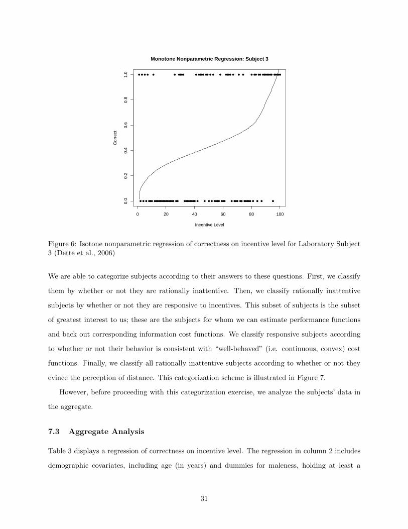
us to infer properties of the cost function that generated it. (Figure 6 provides an example of what

such a performance function might look like.)

In particular, we can answer some of the questions raised in the introduction:

• Do subjects behave in a manner consistent with the predictions of rational inattention?

• Do they respond to incentives?

• Do they exhibit evidence of non-convexities or discontinuities in their cost functions? (Put

differently, are their cost functions not “well-behaved”?)

• Do they evince the perception of distance?

30

●

●●

● ●

●●

● ●●● ● ●

● ●●

● ●●

●

● ●

●

●●

● ●

●

● ●●

● ●

● ●

●●

● ●

●●

●

●

●

●

●

●

●● ●

● ●

●●●●

● ●●

●

●●

●

●●

●● ●

●●

●

● ●● ●

● ● ●●

●●

●

●

●●

●● ● ● ●

●

● ●●●

●

● ● ●

●

0 20 40 60 80 100

0.0

0.2

0.4

0.6

0.8

1.0

Monotone Nonparametric Regression: Subject 3

Incentive Level

Cor

rect

Figure 6: Isotone nonparametric regression of correctness on incentive level for Laboratory Subject3 (Dette et al., 2006)

We are able to categorize subjects according to their answers to these questions. First, we classify

them by whether or not they are rationally inattentive. Then, we classify rationally inattentive

subjects by whether or not they are responsive to incentives. This subset of subjects is the subset

of greatest interest to us; these are the subjects for whom we can estimate performance functions

and back out corresponding information cost functions. We classify responsive subjects according

to whether or not their behavior is consistent with “well-behaved” (i.e. continuous, convex) cost

functions. Finally, we classify all rationally inattentive subjects according to whether or not they

evince the perception of distance. This categorization scheme is illustrated in Figure 7.

However, before proceeding with this categorization exercise, we analyze the subjects’ data in

the aggregate.

7.3 Aggregate Analysis

Table 3 displays a regression of correctness on incentive level. The regression in column 2 includes

demographic covariates, including age (in years) and dummies for maleness, holding at least a

31

Table 3: Regressions of correctness on incentive level and demographic covariates

(1) (2)

Incentive Level 0.003∗∗∗ 0.003∗∗∗

(0.0004) (0.0004)

Age −0.0001(0.006)

Male 0.004(0.056)

Bachelor’s −0.062(0.058)

Econ/Psych/Neuro −0.097∗

(0.054)

$20 Prize 0.023(0.049)

Dots First 0.049(0.052)

Task Number −0.001∗∗∗

(0.0003)

Constant 0.425∗∗∗ 0.498∗∗∗

(0.032) (0.140)

Observations 7900 7900R2 0.03799 0.05635

Note: ∗p<0.1; ∗∗p<0.05; ∗∗∗p<0.01Standard errors clustered on subject.

32

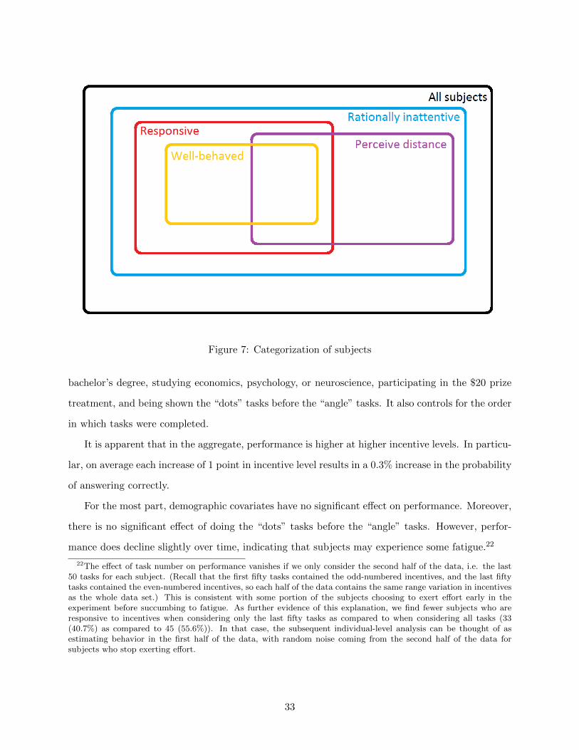
Figure 7: Categorization of subjects

bachelor’s degree, studying economics, psychology, or neuroscience, participating in the $20 prize

treatment, and being shown the “dots” tasks before the “angle” tasks. It also controls for the order

in which tasks were completed.

It is apparent that in the aggregate, performance is higher at higher incentive levels. In particu-

lar, on average each increase of 1 point in incentive level results in a 0.3% increase in the probability

of answering correctly.

For the most part, demographic covariates have no significant effect on performance. Moreover,

there is no significant effect of doing the “dots” tasks before the “angle” tasks. However, perfor-

mance does decline slightly over time, indicating that subjects may experience some fatigue.22

22The effect of task number on performance vanishes if we only consider the second half of the data, i.e. the last50 tasks for each subject. (Recall that the first fifty tasks contained the odd-numbered incentives, and the last fiftytasks contained the even-numbered incentives, so each half of the data contains the same range variation in incentivesas the whole data set.) This is consistent with some portion of the subjects choosing to exert effort early in theexperiment before succumbing to fatigue. As further evidence of this explanation, we find fewer subjects who areresponsive to incentives when considering only the last fifty tasks as compared to when considering all tasks (33(40.7%) as compared to 45 (55.6%)). In that case, the subsequent individual-level analysis can be thought of asestimating behavior in the first half of the data, with random noise coming from the second half of the data forsubjects who stop exerting effort.

33

7.4 Rational Inattentiveness

We now proceed with the individual-level categorization exercise.

Before testing the properties of the subjects’ cost functions, it is necessary to determine whether

there exists a cost function that rationalizes their data in the first place. To that end, we test

the necessary and sufficient “no improving attention cycles” and “no improving action switches”

conditions by testing the equivalent conditions established in Subsection 3.3.

7.4.1 No Improving Attention Cycles

As demonstrated in Proposition 5, a subject satisfies NIAC in our experiment if and only if their

probability of correctly guessing the state is non-decreasing in the reward. This implies that

rationally inattentive subjects have non-decreasing performance functions.

At this point, a clarification is in order. As we showed in Proposition 5, NIAC holds in a set

of uniform guess tasks iff for any pair of decision problems (r1, r2) with r1 > r2, we have that

P ∗(r1) ≥ P ∗(r2). Observationally, this means that the subject had more correct answers under

incentive level r1 than incentive level r2. However, in our experiment each subject is given each

decision problem only once. Therefore, the empirically-observed probabilities of answering each

decision problem correctly are either 0 or 1. If were to apply the NIAC condition directly to our

data, this would mean that the only subjects whose behavior is consistent with NIAC would be

those who always answer incorrectly up to some incentive threshold after which they always answer

correctly. Given the stochasticity of choice under limited attention, this scenario is implausible.

Therefore, rather than strictly interpreting our data as stochastic choice data and making direct

pairwise comparisons of decision problems to test NIAC, we adopt an estimation-based approach.

We estimate the performance function given correctness data and see if this estimate is significantly

different from a non-decreasing function, in which case we reject NIAC. In theory, unless there is

some reward threshold below which the subject is never correct and above which the subject is

always correct, the fit of a monotone performance function can be improved by adding peaks and

troughs. The question, then, that we wish to pose is not whether a non-monotone or decreasing

function can fit the data, but whether we can reject the hypothesis that a non-decreasing function

explains the data.

To test for weak positive monotonicity, we employ a method developed by Doveh et al. (2002)

34

●●

●

●

●

●● ●

●

●●●

●

●● ● ●●●

●

●

●●

●● ● ●

●●

●

●

● ●●● ● ●● ●

●

●● ●● ●● ● ●

●

●●● ●● ●●

●

●●● ●

●

● ●● ●● ●●● ●● ● ● ●●● ●●● ●● ●

●

●

●

● ●

● ●

● ●● ●

●●

●● ●●

0 20 40 60 80 100

0.0

0.2

0.4

0.6

0.8

1.0

Rejects NIAC (Lab Subject 1)

Incentive Level

Cor

rect

●●

● ●

●● ● ● ●● ● ●● ●● ● ●●● ● ●● ●● ●●●

●

●● ●●

●

● ●

●

●

●

● ●

●●

● ●●

●

●●

●

●

● ●

● ● ●

● ●

●● ● ●

●●

●

● ●

● ●

●●

●

●

●

●

● ●● ●

● ● ●●● ●

●

● ● ●

●●

●

●

●

●

●

●●

●● ●

0 20 40 60 80 100

0.0

0.2

0.4

0.6

0.8

1.0

Fails to reject NIAC (Lab Subject 19)

Incentive Level

Cor

rect

Figure 8: Unrestricted cubic polynomial regression of correctness on incentive level for Subjects 1and 19. The former rejects NIAC (and therefore rejects rational inattentiveness), and the latterfails to reject NIAC.

and compare the estimation of an unrestricted cubic polynomial regression of correctness on in-

centive level for each subject to one with a positive derivative restriction. The null hypothesis for

this test is that the response function is monotonic. At the 5% level, we fail to reject positive

monotonicity for 77 out of 81 lab subjects (95.1%).23 Examples of polynomial regressions and

correctness data for two subjects, one who rejects NIAC and one who fails to reject NIAC, are

depicted in Figure 8.

7.4.2 No Improving Action Switches

To test for the second necessary and sufficient condition for rational inattentiveness, NIAS, we

cannot simply simply examine the estimated performance function; we must look at the posterior

probabilities of each state given each response. We employ a bootstrap procedure. For each subject

and response, we calculate the empirically observed distribution of true states, i.e. we calculate

Pr(θ|a). We then simulate 499 bootstrap samples for each distribution.24 If the most common true

23The optimization in the computation of the restricted regression for lab subject 35 failed to converge, and so wedid not perform the test for them. For that subject, a one-tailed t-test of the coefficient on incentive level in a linearregression of correctness on incentive level failed to reject the null of the coefficient being non-negative at the 5%level, and so we classify them as having a non-decreasing performance function.

24Simulating 1 fewer than 500 bootstrap samples ensures that Type I error probabilities are exact (cf. Section 4.6of Davidson and MacKinnon, 2004).

35

state is the one corresponding to the response in at least 5% of samples for each response for a

given subject, then that subject fails to reject NIAS. Overall, we find that 74 out of 81 (91.3%)

laboratory subjects fail to reject NIAS.

Overall, 70 out of 81 (86.4%) laboratory subjects fail to reject both NIAC and NIAS. We refer

to these subjects as “rationally inattentive,” or simply “rational,” subjects.

7.5 Responsiveness

Of the subjects who fail to reject rational inattentiveness, some of them may have flat response

functions, i.e. while they could be rationally inattentive, they do not actually respond to incentives

(within the range of incentives presented to them).

To determine which subjects are responsive to incentives, for each subject who failed to reject

rational inattentiveness, we run a linear weighted least squares regression of correctness on incentive

level and run a one-sided t-test of the coefficient on incentive level with the null of non-positivity,

i.e. non-responsiveness to incentives. However, this is insufficient to capture all responsive subjects;

a subject may be responsive only within a small range of incentives. To address this issue, for each

subject, we repeat this procedure on incentive levels 1 through 50 and on incentive levels 51 through

100.25 If a subject has a significantly positive coefficient on incentive level in any of these three

regressions, then we classify them as responsive.26

At the 5% significance level, 42 out of 70 lab subjects (60.0%) who fail to reject rational inatten-

tiveness are responsive to incentives. Examples of full-sample linear regressions and correctness data

for two subjects, one who fails to reject non-responsiveness and one who rejects non-responsiveness,

are depicted in Figure 9.

7.6 Continuity and Convexity

If the assumptions of Propositions 7, 9, 11, or 12 are satisfied (the cost function is almost strictly

convex, the cost function is a strictly convex function of accuracy, the cost function implies convexity

in the square root of the precision of a normal signal, or the cost function is mutual information,

25Further sample splitting leads to the spurious detection of responsiveness; it leads to some subjects with >95%success being classified as responsive.

26We must consider the full-sample regressions in tandem with the split-sample regressions. If we considered onlythe split-sample regressions, then we would classify subjects who have binary-response performance functions withthresholds around 50 as non-responsive.

36

●

●

●●

● ●

●● ● ●● ●

● ●

● ●● ●

●

●

●

●●

● ● ●

●● ●

●

●

●

● ● ●

●

●

●

●●●

●

● ●● ●● ●● ●●

●

●

●

●● ●

● ●

● ● ●●

●

●

●

●● ●● ●●

●

●●●

●

●● ●● ●

●

●●● ●●●● ●●

●

● ●

●

● ●

●●

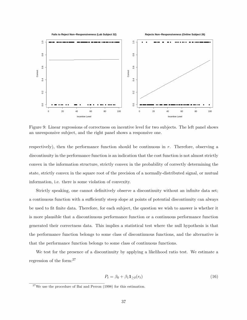
0 20 40 60 80 100

0.0

0.2

0.4

0.6

0.8

1.0

Fails to Reject Non−Responsiveness (Lab Subject 32)

Incentive Level

Cor

rect

●

● ●

● ●●

● ●

● ●

●

● ●

●●● ●● ●

●

● ●

● ● ●

●

●

● ●

●

●

● ●●

●

●

●

●

●● ●● ●● ● ● ●●

●

●●

●

●

●● ●

●

●

●●● ●

● ●

● ● ●●

●

●● ●●

●

●

●● ●

●

● ● ●

● ●●

●

●

●

●

●

● ●

●

●●

●

● ●

●

●

0 20 40 60 80 100

0.0

0.2

0.4

0.6

0.8

1.0

Rejects Non−Responsiveness (Online Subject 26)

Incentive Level

Cor

rect

Figure 9: Linear regressions of correctness on incentive level for two subjects. The left panel showsan unresponsive subject, and the right panel shows a responsive one.

respectively), then the performance function should be continuous in r. Therefore, observing a

discontinuity in the performance function is an indication that the cost function is not almost strictly

convex in the information structure, strictly convex in the probability of correctly determining the

state, strictly convex in the square root of the precision of a normally-distributed signal, or mutual

information, i.e. there is some violation of convexity.

Strictly speaking, one cannot definitively observe a discontinuity without an infinite data set;

a continuous function with a sufficiently steep slope at points of potential discontinuity can always

be used to fit finite data. Therefore, for each subject, the question we wish to answer is whether it

is more plausible that a discontinuous performance function or a continuous performance function

generated their correctness data. This implies a statistical test where the null hypothesis is that

the performance function belongs to some class of discontinuous functions, and the alternative is

that the performance function belongs to some class of continuous functions.

We test for the presence of a discontinuity by applying a likelihood ratio test. We estimate a

regression of the form:27

Pt = β0 + β11≥δ(rt) (16)

27We use the procedure of Bai and Perron (1998) for this estimation.

37

where β0, β1, and δ are the parameters to be estimated and compare its likelihood to an estimation

of the following logistic relationship:

Pt =β1

1 + exp(−λ(rt − δ))+ β0 (17)

It can be shown that (16) is the pointwise limit of (17) as λ goes to infinity. Therefore, (16) can be

seen as the restricted null model, and a likelihood ratio test comparing these models is effectively

a test of the null hypothesis that λ = ∞, i.e. it is a test against the null hypothesis that there is

a jump discontinuity. Since we are performing this test only on responsive subjects, our estimates

of β1 for each subject should be positive, and therefore this procedure should not detect spurious

downward jump discontinuities for those subjects.28

Using this test, at the 5% level we cannot reject that 29 out of 42 responsive lab subjects

(69.0%) have discontinuities in their response functions.

7.7 Perceptual Distance

A mutual-information cost function, among others, does not embed a concept of perpetual distance.

What that means in our experiment is that mutual information predicts that given a true state

of nature, each incorrect response is equally likely. For example, if the true number of dots is 39,

reporting 42 should be just as likely as reporting 38, even though the difference between 42 and 39

is 3, whereas the difference between 38 and 39 is 1. Taking absolute value as the natural metric on

{38, . . . , 42}, this means that if a subject evinces perceptual distance, then given a true state of 39,

she should be more likely to report 38 than 42.

For each subject and trial t, we compute the error distance ρ(at, θt) = |at−θt|. In our experiment

this distance in an integer in {1, 2, 3, 4}. In order to test this symmetry prediction of the mutual

information cost function, for each responsive subject we compute the distribution of error distances

that mutual information would predict, given the empirically observed distribution of true states

and the subject’s overall accuracy rate. We then compare the empirically observed distribution of

28Several procedures for detecting discontinuities have been proposed in the econometric literature. See, for exam-ple, Andrews (1993), Andrews and Ploberger (1994), Bai and Perron (1998), and Porter and Yu (2015). All of theseprocedures are designed to detect both positive and negative jump discontinuities, and so they are vulnerable to thedetection of spurious negative jumps in our setting. A clarification is in order here. Bai and Perron (1998) proposeboth an estimation procedure and a testing procedure for models with structural breaks with unknown discontinuitypoints. We use their estimation procedure to estimate (16), but we do not use their testing procedure.

38

Table 4: Categorization of subjects

Category Of All Subjects Of R.I. Subjects Of Resp. Subjects Of P.D. SubjectsAll subjects 81 (100%) — — —R.I. subjects 70 (86.4%) 70 (100%) — —Resp. subjects /// 42 (60.0%) 42 (100%) 26 (57.8%)W.B. subjects /// /// 13 (31.0%) 8 (17.8%)P.D. subjects /// 45 (64.3%) 26 (61.9%) 45 (100%)

Note: “R.I.” = rationally inattentive; “Resp.” = responsive; “W.B.” = well-behaved, i.e. subjects whosebehavior is consistent with continuous, convex cost functions; “P.D. Subjects” = subjects who evince theperception of distance. — denotes that the column category is a subset of the row category, and /// denotesthat the row category is defined only on a subset of the column category.

error distances to this distribution using a chi-square test.

At the 5% level, we find that 26 out of 42 responsive lab subjects (61.9%) have a distribution

of mistakes that evinces the perception of distance. Of course, the notion that perceptual distance

matters for error distance distributions is not limited to responsive subjects; mutual information

implies responsiveness (i.e. a strictly increasing performance function), so subjects who are not

responsive have already rejected mutual information for other reasons. But as a test of the general

notion that each possible mistake is equally likely given an true state of nature, it is worth running

these tests on the entire pool of rationally inattentive subjects. At the 5% level, we find that 45

out of 70 rationally inattentive lab subjects (64.3%) reject this hypothesis.

7.8 Summary of Categorization

Table 4 summarizes the results of preceding subsections.29 Each cell indicates the number and

percentage of row category subjects in the column category. It should be noted that the vast

majority (86.4%) of subjects are rationally inattentive, and moreover, most rationally inattentive

subjects are responsive (60.0%). Also of note is the fact that most rationally inattentive subjects

evince the perception of distance (64.3%).

8 Model Selection

In this section, for each responsive subject we fit several possible parametric functional forms for

performance functions, each of which can be generated by some cost function. These models are

29 blah

39

Table 5: Performance functions estimated and their corresponding cost functions

Cost Function Performance Function Estimation

1 Very high or low marginal or absolute costs Constant OLS

2 Dual-process or concave Binary BP98

3 Quadratic in accuracy Affine WLS

4 Discontinuous or has non-convexity Affine with break BP98

5 Integral of inverse of 2nd degree polynomial in accuracy 2nd degree polynomial WLS

6 Integral of inverse of 3rd degree polynomial in accuracy 3rd degree polynomial WLS

7 Mutual information or logit cost Logistic MLE

8 Normal signals with linear cost of precision Concave MLE

Note: BP98 = Bai and Perron (1998)

listed in Table 5.30

8.1 Description of Models

We now describe each of these models.

Model 1. Since we perform this model selection exercise only on responsive subjects, we fit

a constant performance function as a robustness check. A flat performance function obtains when

there is a single performance level such that a subject’s cost for higher performance is too high to

warrant improvement for any incentive level and their savings in terms of information costs are too

low to warrant lowering their performance at any incentive level.

Models 2 and 4. These models have discontinuous performance functions, implying by Propo-

sition 7, 9, 11, or 12 that the corresponding cost functions have some violation of convexity or

continuity. We estimate Model 2 by:

Pt = β0 + β11≥δ(rt) (18)

and Model 4 by:

Pt = β0 + β11≥δ(rt) + β2rt + β3rt · 1≥δ(rt) (19)

where δ is the location of the discontinuity, using the linear structural change estimation technique

30The reason that we do not consider the channel capacity cost function is because since the prior distribution inour task is uniform, channel capacity would be consistent with the same behavior as mutual information (cf. Section1.2.3 of Woodford, 2012)

40

of Bai and Perron (1998).

Given the estimates of (18), we can recover the parameters of the corresponding fixed-cost

information cost function (9). It is clear that q = β0 and q = β0 + β1. As shown in Subsection

5.4, the location δ of the discontinuity in the performance function is given by κq−q . Therefore,

κ = δ(β1 − β0).

A performance function of the form of (18) could also be obtained from a concave information

cost function. To illustrate, consider for simplicity a subject who has a cost function K that is

concave in performance, as depicted in Figure 10.

P10.2

K(P )

�������������������������� r1P

�������������

��

���

���

���

��

r2P

Figure 10: Concave costs

Net payoffs are maximized when the positive distance between gross payoffs and costs is largest.

For low reward levels (such as r1), this happens at the no-information performance level, 0.2. For

high reward levels (such as r2), this happens at the full-information performance level, 1. In this

manner, a binary performance function obtains, with the subject acquiring no information if the

41

incentive is low and acquiring full information if the incentive level is high.

Model 4 nests Model 2, and so it can correspond to a wider class of cost functions, including

those of similar form to (9), but with two convex components as opposed to only two admissible

information structures.

Models 3, 5, and 6. These models estimate continuous performance functions, and since

these models are estimated only for responsive subjects, these estimated performance functions

should be increasing. As explained in Subsection 5.4, this means we can recover the corresponding

information cost functions by inverting and taking the antiderivative of the estimated performance

functions. While the quadratic and cubic performance functions of Models 5 and 6 do not have very

simple closed forms for their corresponding cost functions, Model 3’s corresponding cost function

can be easily recovered from its estimate:

Pt = β0 + β1rt (20)

In this case, inverting and integrating the performance function gives us the performance-dependent

cost function K(P ), where:

K(P ) =1

2β1

(P 2 − 0.04)− β0

β1

(P − 0.2) (21)

assuming that K(

1n

)= 0, i.e. that acquiring no information entails no cost.

Model 7. As we showed in Proposition 9, a mutual information cost function implies a logistic

performance function, which we can estimate with:

Pt =1

4 exp(− rtα

)+ 1

(22)

However, Proposition 9 also implies that if a subject evinces the perception distance, then they

cannot have a mutual information cost function. To reconcile logistic performance with perceptual

distance, one can assume that the subject actually has a performance-dependent cost function and

apply the inversion-and-integration procedure of Subsection 5.4. This gives the following “logit”

42

Table 6: Model Selection for Responsive Subjects

Model Binary (2) Logistic (7) Concave (8)

Number of Subjects 10 (23.8%) 26 (61.9%) 6 (14.3%)

cost function (assuming that acquiring no information entails no cost):

K(P ) = α

(P ln

(4P

1− P

)+ ln(1− P ) + ln(1.25)

)(23)

Model 8. For this model, we assume that the subject receives normal signals with precision ζ2

and the cost of a signal is linear in precision, as in the numerical example of Section 5 of Verrecchia

(1982). Therefore, the cost of a signal is K(ζ) = αζ2. α is the parameter we wish to estimate for

each subject.

The performance function for this cost function in our experiment is (from (14)):

Pt =8

5Φ

(ζ∗(rt)

2

)− 3

5(24)

where ζ∗ solves the first-order condition of (14) for our experiment:

αζ∗ =2

5rtφ

(ζ∗

2

)(25)

8.2 Comparison of Models

We now run a “horse race” to determine which model is the best fit for each subject. Since the

models are non-nested and are estimated using different estimation techniques, we cannot use a

traditional auxiliary regression method for model selection. To determine which model is the best

fit for each responsive subject, we estimate each model for each such subject and then compare

their Akaike Information Criteria (AIC) (cf. Section 8.5 of Cameron and Trivedi, 2005), selecting

the model that yields the lowest AIC. The results of this selection are given in Table 6.

All responsive subjects are best fit by binary (fixed costs), logistic (mutual information or “logit”

performance dependence), or concave performance (normal signals with linear precision cost). The

first implies some sort of non-convexity or discontinuity in the cost function, whereas the latter two

are consistent with convex cost functions. Figures 11, 12, and 13 show what these performance

43

Table 7: Average AIC and Rank for Estimated Models

Model AIC Rank

1 131.165 6.548

2 114.060 2.143

3 117.832 3.524

4 119.982 4.905

5 131.123 5.595

6 132.929 6.643

7 116.008 2.308

8 121.967 4.333

functions look like for three subjects.

Table 7 shows the average estimated AIC and rank of each model in the “horse race.”31 Models

2 (binary), 3 (affine), and 7 (logistic) have the lowest ranks on average. Flexible polynomial fits

do quite poorly; the average rank of a cubic performance function (Model 6) is higher than that of

the constant performance model (Model 1).

Note that the average AIC and rank for Model 7, the logistic performance function, is lower

than that of Model 2, the binary performance function, despite the fact that significantly more

subjects are best fit by Model 7 than by Model 2. This indicates that the binary model is a decent

fit when the best-fitting model is logistic, but the logistic model is a poor fit when the best-fitting

model is binary. When the logistic model is the best fit, the average rank of the binary model is

2.577; however, when the binary model is the best fit, the average rank of the logistic model is

4.100. Note also that the average rank of Model 8 (normal signals with linear precision cost) is

fairly high at 4.333. This indicates that when Model 8 is not the best fit for a subject, it is a poor

fit.

9 Additional Results

9.1 Categorization and Demographics

In this subsection, we determine the extent to which demographic covariates predict the catego-

rization of subjects as rationally inattentive and responsive, as well as whether their best-fitting

performance function is binary or logistic.

31A lower rank implies a lower AIC and therefore a better fit.

44

● ●● ● ●● ●● ●● ●●●● ● ● ●● ●● ●● ●● ●● ●● ● ● ●● ● ● ●● ●●● ● ●● ●●● ●●● ●

●

● ●

● ●

● ●

●

●

●

●

●

● ●●●●

● ● ●

●● ●

●

●

●

●●●● ● ●●

●

●

●●

●

●

●

●

●

●

●

●●

●

●

●●

●

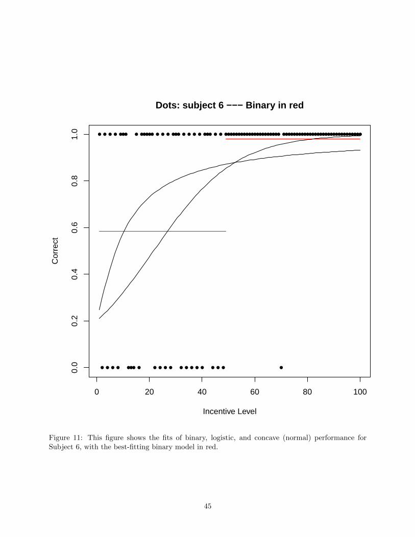
0 20 40 60 80 100

0.0

0.2

0.4

0.6

0.8

1.0

Dots: subject 6 −−− Binary in red

Incentive Level

Cor

rect

Figure 11: This figure shows the fits of binary, logistic, and concave (normal) performance forSubject 6, with the best-fitting binary model in red.

45

● ●●

●

●

●●

●

● ●●● ●

●

● ●●

●

●● ●● ●

●

●

●●

●●

●

●● ●

● ●

● ● ●

●●●

●

●

●● ●●

●● ●●

● ● ●●● ●●

●● ●●

●●

●●

●

● ●

● ●● ●●

●● ●

● ●

●

●

●●

●

●

●● ● ●●●

●

●● ●●●

●

●

●

0 20 40 60 80 100

0.0

0.2

0.4

0.6

0.8

1.0

Dots: subject 14 −−− Logistic in red

Incentive Level

Cor

rect

Figure 12: This figure shows the fits of binary, logistic, and concave (normal) performance forSubject 14, with the best-fitting logistic model in red.

46

●

●

●

●● ●

●● ●● ●

●

● ●

●

● ●

● ●

●●

●● ●

●

●

●

●

●

●●

●● ●● ● ●

● ●

●● ●●

●●

● ●

● ●

● ● ●

●

●

●

● ●

●

● ●

●

●●

●

● ●

●

●● ●

● ●

●●

● ●

●●

●

●

●●

●●●

●

● ●● ● ●●

● ● ●●●

●

●

●

0 20 40 60 80 100

0.0

0.2

0.4

0.6

0.8

1.0

Dots: subject 66 −−− Concave (Normal) in red

Incentive Level

Cor

rect

Figure 13: This figure shows the fits of binary, logistic, and concave (normal) performance forSubject 66, with the best-fitting concave (normal) model in red.

47

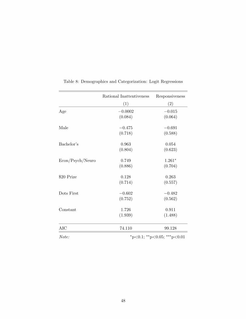
Table 8: Demographics and Categorization: Logit Regressions

Rational Inattentiveness Responsiveness

(1) (2)

Age −0.0002 −0.015(0.084) (0.064)

Male −0.475 −0.691(0.718) (0.588)

Bachelor’s 0.963 0.054(0.804) (0.623)

Econ/Psych/Neuro 0.749 1.261∗

(0.886) (0.704)

$20 Prize 0.128 0.263(0.714) (0.557)

Dots First −0.602 −0.482(0.752) (0.562)

Constant 1.726 0.911(1.939) (1.488)

AIC 74.110 99.128

Note: ∗p<0.1; ∗∗p<0.05; ∗∗∗p<0.01

48

9.1.1 Rational Inattentiveness

To determine the extent to which demographics predict a failure to reject NIAC, we run a logit

regression of an indicator for rational inattentiveness on demographic covariates. These covariates

are age, an indicator for being male, an indicator for having attained at least a bachelor’s degree, an

indicator for studying economics, psychology, or neuroscience, an indicator for participating in the

$20 prize treatment, and an indicator for having done the dots tasks first. We display the results

of this regression in column 1 of Table 8.

Demographic covariates do not seem to be predictive of rational inattentiveness in this particular

subject pool. Neither do experimental variables, such as the higher prize and completing the

dots tasks first. This suggests that for a given set of tasks, rational inattentiveness is an innate

characteristic that is not well captured by demographics, and moreover, it may be difficult to

manipulate experimentally.

9.1.2 Responsiveness

To determine the extent to which demographics predict responsiveness, we run a logit regression

of an indicator for responsiveness on demographic covariates for the subjects who fail to reject

rational inattentiveness. We display the results of this regression in column 2 of Table 8.

As is the case with rational inattentiveness, demographic covariates are not significant predictors

of responsiveness.

9.1.3 Cost Functions

To determine the extent to which demographics predict model selection, we run a multinomial

logit regression of the best-fitting model on the same set of demographic covariates as in previous

subsubsections, with logistic performance (Model 7, mutual-information costs) as the baseline. This

regression shows us the extent to which these demographic factors affect the likelihood of selecting

a model that implies a non-convexity or discontinuity in the cost function over one that is consistent

with convexity. We display the results of this regression in Table 9.

As is the case with previous demographic regressions, demographic factors are not significant

predictors. This seems to indicate that not only is rational inattentiveness not well captured by

demographics, so is the nature of one’s cost function for information in a given task.

49

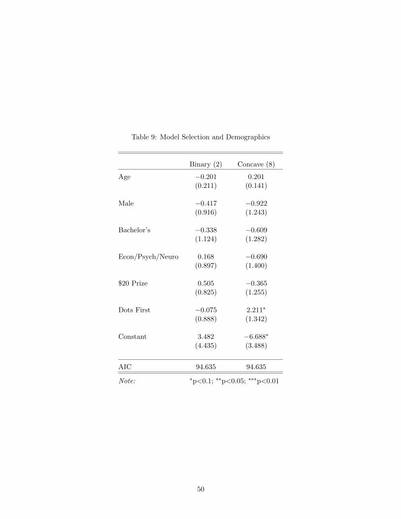
Table 9: Model Selection and Demographics

Binary (2) Concave (8)

Age −0.201 0.201(0.211) (0.141)

Male −0.417 −0.922(0.916) (1.243)

Bachelor’s −0.338 −0.609(1.124) (1.282)

Econ/Psych/Neuro 0.168 −0.690(0.897) (1.400)

$20 Prize 0.505 −0.365(0.825) (1.255)

Dots First −0.075 2.211∗

(0.888) (1.342)

Constant 3.482 −6.688∗

(4.435) (3.488)

AIC 94.635 94.635

Note: ∗p<0.1; ∗∗p<0.05; ∗∗∗p<0.01

50

9.2 Reaction Times

In addition to data on subject responses, we also collected data on how much time subjects spent

on each task. We call this the reaction time.

9.2.1 Time and Attention

Thus far, in this paper, we have remained agnostic about the exact nature of what attention

comprises, and by corollary, we have remained agnostic about the exact source of information

costs. One possibility is that attention can be decomposed into a quantity component — time

spent on a task — and a quality component — how much effort is exerted during that time. Here,

we provide some suggestive evidence that attention indeed has a quantity component.

Table 10: Linear regression of reaction time on incentive level

Reaction Time

Incentive Level 0.178∗∗∗

(0.017)

Constant 14.159∗∗∗

(1.378)

Observations 8100R2 0.059

Note: ∗p<0.1; ∗∗p<0.05; ∗∗∗p<0.01Standard errors clustered on subject.

Tables 10 and 11 display linear regressions of reaction time on incentive level and correctness on

incentive level, respectively, aggregating over the subject pool. The coefficients on the dependent

variables in both regressions are positive and significant. In the case of the first regression, this

indicates that subjects respond to higher incentives by increasing the quantity of attention paid to

the task at hand. In the case of the second regression, this indicates that increasing the quantity

of attention results in higher performance; this is the speed-accuracy trade-off commonly noted in

the literature on perceptual psychology (e.g. Schouten and Bekker, 1967).

51

Table 11: Linear regression of correctness on reaction time

Correctness

Reaction Time 0.007∗∗∗

(0.001)

Constant 0.427∗∗∗

(0.036)

Observations 8100R2 0.096

Note: ∗p<0.1; ∗∗p<0.05; ∗∗∗p<0.01Standard errors clustered on subject.

9.2.2 Dual-Process Mechansims

As we showed in Subsection 8.2, choice data for approximately one-third of responsive subjects are

best fit by binary performance functions. This suggests that these subjects employ two different

strategies for determining the number of dots on the screen — one for low incentives, and one for

high incentives. In this subsubsection, we provide further suggestive evidence for this hypothesis.

Figure 14 shows the histogram of reaction time on every task for the subject population. The

distribution of reaction times is clearly bimodal. There are at least two possible, non-mutually

exclusive explanations for this. One is that some portion of the subjects simply do not exert any

effort on the task and make a response at the earliest opportunity, while others exert effort in

acquiring information. Another is that subjects have binary performance functions, choosing not

to spend time acquiring information for some incentive levels but choosing to do so for others.

The fact that a significant portion of subjects are best fit by binary performance functions

provides an explanation for the pattern observed in Figure 14. Some subjects make snap decisions

when confronted with low incentives but take the time to acquire information at higher incentive

levels. This can be seen more clearly in Figure 15, which shows the histogram of reaction time on

every task for responsive subjects only. Observe that this histogram is also clearly bimodal.

To interrogate this question further, we run the dip test of Hartigan and Hartigan (1985) on

each subject’s reaction times to determine which ones have multimodal reaction time distributions.

We can reject the null of unimodality at the 5% level for 26 out of 42 responsive subjects (61.9%).

52

Figure 14: Histogram of reaction times for all subjects

53

Figure 15: Histogram of reaction times for responsive subjects

54

This is more than the number of responsive subjects whose data are best fit by binary performance

functions, meaning that some subjects with logistic or concave performance functions do not have

unimodal reaction time distributions. This suggests that rather than continuously adjusting their

quantity of attention as incentive levels increase, some subjects randomize between paying a high

quantity and a low quantity of attention, and the probability of paying a high quantity of attention

increases as incentive levels increase.

This evidence implies that for a large portion of the subject pool (61.9%), there are two

information-acquisition processes that they can employ in this task. Still, there is a significant

portion of the pool (38.1%) that is apparently able to adjust their quantity of attention continu-

ously. As was the case with previous categorizations of subjects, there is significant heterogeneity.

10 Application to the Delegation of Investment

The characteristics of the decision-maker’s cost function can obviously have effects on her own

decisions. But as we show in this section, these characteristics can also have effects on economically-

relevant outcomes when there is strategic interaction.

In order to demonstrate this notion, let us consider a situation in which an investor is deciding

which of n options to invest in, and he cannot split his investment across options. Suppose that

only one of these options can be a winner, in which case an investment in it will pay a net return of

x. Losing opportunities pay a net return of zero. This setup has the relevant features of a situation

where the success of an investment depends on the outcome of a contest. Many economic situations,

such as competing to be granted development rights by the government for a plot of land, take the

form of contests. Another salient example is a patent race, where various firms compete to be the

first to patent an invention, such as a drug or a piece of technology.

Suppose that the investor wishes to delegate researching these options to an expert. This is a

common occurrence in reality; people frequently solicit the services of financial advisors, presumably

because it is prohibitively difficult or costly for laypeople to research investment opportunities

themselves, while financial advisors who are trained to seek and interpret financial information can

research these opportunities at a much lower cost.

We can analyze this situation in a simple principal-agent framework, where the investor is

55

the principal and the expert is the agent.32 The agent acquires information about the available

investment opportunities at a cost and selects one of the options on the principal’s behalf. Suppose

that the principal employs the agent with a contract that pays r if the agent correctly selects the

winner and zero otherwise.33 Furthermore, suppose that a priori, each option is equally likely to

be the winner. Then, the agent’s problem can be represented as a uniform guess task, with the

reward for a correct answer being r. Consequently, the principal’s problem is

maxr∈[0,x]

(x− r)P ∗(r) (26)

where P ∗(r) is the agent’s performance function.

As we established in Proposition 5, if the agent is rationally inattentive, then her performance

function is (weakly) increasing. Thus, the principal faces a trade-off between incentivizing the agent

to acquire better information and giving up a larger portion of his net return upon success. The

exact nature of this trade-off depends on the potential net return x and the agent’s information

cost function. In the following subsections, we analyze the properties of the principal’s optimal

payment strategy r∗ under two of the cost function models fit by our data: fixed costs and mutual

information.34

10.1 Fixed Costs

Suppose the agent has a fixed cost κ for acquiring information. If she pays the cost, then she learns

the winner with certainty. If not, then she learns nothing about the identity of the winner. Thus,

she chooses to acquire information if r − κ ≥ rn , i.e. when r ≥ κn

n−1 .

Therefore, if x < κnn−1 , then the reward required to incentivize the agent to acquire information

is higher than the potential net return, so the principal is better off not hiring the agent at all

32We use male pronouns for the principal and female pronouns for the agent.33This type of contract is optimal for the principal if we assume that (a) there is a limited-liability constraint

so that the agent cannot earn a negative payoff in any state of the world, which implies that the principal cannot“sell the firm” to the agent; and (b) the agent’s cost of an uninformative information structure is zero. As CD15demonstrate, the latter assumption is without loss of generality; it is not a testable restriction on information costfunctions.

34We do not present the model under the assumption of normally-distributed signals here, because it implies thatthe options have some existing ranking, and it is not clear what it means for the options to be “equidistant” from eachother. That being said, it can be shown that if options are ranked and equidistant, then normal signals with convexprecision costs imply that that the principal’s optimal payment strategy is continuous in potential net rewards. Inany case, if the normal-signals model is excluded from consideration, then in our data, the best-fitting model for eachsubject is either binary (fixed costs) or logistic (mutual information). (Results available from the authors on request.)

56

and simply picking an option at random. If instead x ≥ κnn−1 , then the principal could incentivize

information acquisition by paying as little as r = κnn−1 . To ensure that this payment is not so high

than the principal could do better on his own, he requires that xn ≤ x − κn

n−1 , which holds if and

only if x ≥ κn2

(n−1)2. But since κn

n−1 <κn2

(n−1)2, the principal will not hire the agent unless x ≥ κn2

(n−1)2.

To summarize: if x < κn2

(n−1)2, then the principal does not hire the agent and selects an option

at random. If x ≥ κn2

(n−1)2, then the principal hires the agent and gives her a payment of κn

n−1 , and

the agent picks the winner with certainty. This implies a discontinuity in the principal’s payment

as a function of the potential net return x.

10.2 Mutual Information

Suppose the agent has a mutual-information cost function with cost parameter α. Then, since her

performance function is logistic (see Proposition 9), the principal chooses r to maximize:

x− r(n− 1) exp

(− rα

)+ 1

(27)

If this maximand is strictly quasiconcave, then this problem has a unique solution for each x,

and the maximum theorem guarantees that the principal’s optimal choice of r∗ is continuous in x.

This turns out to be the case.

Proposition 13. If the agent has a mutual information cost function, then the principal’s optimal

payment strategy r∗(x) is continuous.

To provide an example, suppose n = 5, α = 1, and x ∈ [5, 100]. As shown by Proposition 13, the

maximand (27) is strictly quasiconcave in r (see Figure 16 for an example). For these parameters,

r∗(x) is continuous and increasing, as shown in Figure 17.

These examples demonstrate that the characteristics of an agent’s information cost function

can affect how a principal’s decisions change with the parameters of his environment. Some cost

functions, like the fixed-cost function described above, induce the principal to pay for information

acquisition only when the potential net return is sufficiently high. Others, like the mutual informa-

tion cost function, cause the principal to vary his payment continuously with changing potential

net returns.

57

Figure 16: Principal’s expected payoff as a function of payment for x = 20

Figure 17: Optimal payment as a function of potential net return

58

11 Conclusion

This paper has provided a framework for testing properties of information cost functions in models

of rational inattention. To the extent that the presence or absence of characteristics such as

continuity, convexity, and perceptual distance can have an impact on people’s decisions, it is worth

knowing whether their cost functions satisfy such conditions. Decision-makers’ cost functions are

not directly observable, so instead we must infer their characteristics from observed behavior. We

conducted a set of experiments that allowed us to implement these tests.

These experiments reveal substantial heterogeneity in behavior. Most subjects are rationally

inattentive, but only about half are actually responsive to incentives. Many subjects have behavior

that is consistent with continuous, convex cost functions, and many subjects have behavior that

evince the perception of distance as well. Moreover, there is considerable heterogeneity in whether

or not subjects finely adjust their quantity of attention, though this heterogeneity is limited to

three classes of cost functions: fixed costs, mutual information, and normal signals are the only

best-fitting cost functions for responsive subjects in terms of performance.

This has implications for modeling. In models where agents acquire information, it is perhaps a

better reflection of reality to allow for some heterogeneity in their fundamentals. In particular, one

may want to model some portion of the population as non-responsive to incentives for information

acquisition, or among responsive incentives, one could designate some as having fixed costs for

information acquisition and others as having mutual-information or normal-signal cost functions.

Two possible avenues for future experimental research present themselves. The first is to obtain

more detailed data on what subjects are actually paying attention to. Eyetracking has already been

used in several economics experiments (e.g. Wang et al., 2010; Krajbich et al., 2010; Arieli et al.,

2011) to track subjects’ gaze, which allows researchers to find out what visual information the

subjects are acquiring. Tracking subjects’ mouse movements in computer-based tasks (e.g. Gabaix

et al., 2006) is another potential approach. The second is to use choice data in tandem with reaction

time data to fit models of dynamic information acquisition. This would also allow researchers to

determine to what extent subjects trade off speed and accuracy in their decision-making.

59

Appendix A: Proofs

Proof of Proposition 1

Proof. The ‘if’ direction is obvious, since our model generalizes CD15 with finite action sets.

The ‘only if’ direction can be seen as follows. Suppose {(Ui, θi, ai)} can be rationalized by (2)

with some cost function C(π,Q). Since there are finitely many decision problems, C is pinned down

for a finite set of points (i.e. a closed set), and so by the Tietze extension theorem (cf. Rudin,

1974, pg. 422), it may be assumed continuous. Define QγQ to be set of information structures that

induce posterior γQ, and define C(π,Q) := minR∈QγQ

C(π,R), assuming it is well-defined. γQ always

induces the same maximum gross payoff, no matter which information structure in QγQ generated

it. Therefore, since the DM is a payoff maximizer, for each distribution of posteriors she generates,

she will always select the lowest-cost method of doing so. This implies that behavior that can be

rationalized by C can also be rationalized by C, which obviously satisfies cost equivalence.

Now we must verify that C is actually well-defined. Let b : Q −→ ∆(∆(Θ)) be the function

that maps an information structure to the distribution of posteriors it induces. First, we must

show that b is continuous when ∆(∆(Θ)) is equipped with the weak-∗ topology, i.e. the topology

of weak convergence of measure.

By Bayes’ rule, Supp(b(Q)) ={(

πsqs,k∑nl=1 πlql,k

)ns=1

∣∣∣k ∈ {1, . . . |M |},∑nl=1 πlql,k > 0

}, and each

element ζ ∈ Supp(b(Q)) is induced with probability∑

k∈Qζ∑n

l=1 πlql,k, where Qζ is the set of

columns of Q that generate the posterior ζ.

Consider a sequence of information structures Q1, Q2, . . . ∈ Q converging to Q. We must

show that limj→∞

b(Qj) = b(Q) (in the sense of weak convergence of measure). By Theorem 25.8 of

Billingsley (1995), this is equivalent to showing that limj→∞

b(Qj)(X) = b(Q)(X) for all continuity

sets X in the Borel σ-algebra of ∆(Θ).35

Since X is a continuity set, ∂X∩Supp(b(Q)) = ∅. There are two cases. Either X∩Supp(b(Q)) =

∅ or int(X) ∩ Supp(b(Q)) 6= ∅.

Case 1: X ∩ Supp(b(Q)) = ∅. If ∃ J ∈ N such that b(Qj)(X) = 0 ∀ j > J , then clearly

limj→∞

b(Qj)(X) = b(Q)(X) = 0. If not, then ∀ J ∈ N, ∃ j > J such that X ∩ Supp(b(Qj)) 6= ∅.

Suppose, for a contradiction, that limj→∞

b(Qj)(X) 6= 0. Then ∃ ε > 0 such that ∀ J ∈ N, ∃ j > J such

35A continuity set is a set X whose boundary ∂X has measure zero.

60

that b(Qj)(X) > ε. Therefore, there must exist a subsequence Qjh such that((

πsqs,k∑nl=1 πlql,k

)ns=1

)jh

converges in cl(X) for some k.36 If it converges to a point in int(X), then this contradicts the fact

that b(Q)(X) = 0. If it converges to a point in ∂X, then b(Q)(∂X) > 0, contradicting the fact that

X is a continuity set. Thus, limj→∞

b(Qj)(X) = b(Q)(X).

Case 2: int(X) ∩ Supp(b(Q)) 6= ∅. Note that since (Qj) is a convergent sequence, each entry

of the matrices in (Qj) also defines a convergent sequence. Then each ((zk)j) := ((∑n

l=1 πlql,k)j)

is a convergent sequence with limit zk, and each ((yk)j) :=

(((πsqs,k∑nl=1 πlql,k

)ns=1

)j

)either converges

to some limit yk (for zk > 0) or else has an undefined limit (when zk = 0).37 Since they are

continuous functions of the entries of π and (Qj), and because (Qj) is convergent, yk =(

πsqs,k∑nl=1 πlql,k

)(when it exists) and zk =

∑nl=1 πlql,k, where the entries ql,k are taken from Q. Consider the set

K ⊆ {1, . . . ,M} such that {((yk)j)|k ∈ K} is the collection of sequences that converge to points in

int(X). Then, because int(X) is open, ∀ ε > 0 and ∀ k ∈ K, ∃Nk such that ∀ j > Nk, (yk)j ∈ int(X).

Let N = maxk∈K

Nk. Then ∀ j > N, b(Qj)(X) ≥ (∑

k∈K(∑n

l=1 πlql,k))j .

We now show that b(Qj)(X)−∑

k∈K(∑n

l=1 πlql,k)j goes to zero as j grows large. Suppose there

does not exist J ∈ N such that this sequence has the value 0 ∀ j > J . Then there must exist a

subsequence (Qjh) such that b(Qjh)(X)−∑

k∈K(∑n

l=1 πlql,k)jh > 0 for all jh. Then for each jh, there

is some k′�∈K such that (yk′)jh ∈ Supp(b(Qjh)). Because |M | is finite, we may assume that this k′

is fixed. If ((yk′)jh) is convergent, it must converge in cl(X). If yk′ ∈ int(X), then this contradicts

the fact that k�∈K. If yk′ ∈ ∂X, then this contradicts the fact that X is a continuity set. If ((yk′)jh)

has no defined limit, then zk′ = 0. Therefore, limh→∞

[b(Qjh)(X)−

∑k∈K(

∑nl=1 πlql,k)jh

]= 0.

This establishes the continuity of b. Therefore, for a given γ with finite support in ∆(∆(Θ)),

b−1({γ}) is closed (since singletons are closed). Because b−1({γ}) ⊆ Q and Q is a bounded subset

of Rn × R|M |, then by the Heine-Borel theorem, b−1({γ}) is compact.

In particular QγQ is compact, and since C is continuous (fixing π), by the Weierstrass theorem,

it attains its minimum on QγQ . Therefore, C is well-defined. This concludes the proof.

36We can take k fixed here because even if we construct a subsequence where the sequence of posteriors is constructedby different columns of Qjh for different sequence elements, we can merely take a subsequence of that subsequence,but with k fixed.

37It is possible that (yk)j′ maybe be undefined for some k and j′. This occurs when (zk)j′ = 0. If there are finitelymany such j′, then we can simply consider a sequence (Qj) with these j′ removed. If there are infinitely many such j′,then (zk)j must converge to zero. Therefore, WLOG, either (Qj) is such that (zk)j 6= 0 ∀ j, k and possibly convergesto zero, or (zk)j definitely converges to zero.

61

Proof of Proposition 3

Proof. First we show that we may assume a fixed decision matrix D such that:

D :=

I|A|

1 0 · · · 0

.... . .

. . ....

1 0 · · · 0

(28)

where I|A| is the identity matrix of dimension |A|×|A| and the lower block of D has dimension

(|M |−|A|)× |A|.

Given Q ∈ Q, select a decision matrix D such that the gross payoff tr(QDUΠ) is maximized.

Since the gross payoff is linear in the entries of D, its entries may be chosen so that all of its nonzero

entries are 1, WLOG. Consider the mapping δ : {1, . . . , |M |} −→ {1, . . . , |A|} so that δ(j) is the 1

entry in the j-th row of D. The signal (and associated posterior) induced by the j-th column of Q

result in action aδ(j) being taken.

Now consider Q′ constructed from Q and δ in the following manner. For k ∈ {1, . . . , |A|}, the

k-th column of Q′ is∑

j∈δ−1(k) q•,j , where q•,j is the j-th column of Q and empty sums are taken

to be columns of zeroes. For k > |A|, the columns of Q′ are all zeroes.

(Q,D) and (Q′, D) imply the same Pr(a|θ) for each a ∈ A, θ ∈ Θ, since the (i, j)-th entry of

Q′D is q′i,j =∑

k∈δ−1(j) qi,k. For j ≤ |A|, q′i,j = Pr(aj |θi), since under D, action j is taken only

when signal j is received. Furthermore, for j ≤ |A|,∑

k∈δ−1(j) qi,k = Pr(aj |θi), since under D,

action j is taken if and only if a signal in δ−1(j) is received. Thus, tr(QDUΠ) = tr(Q′DUΠ), i.e.

the gross payoffs are the same under either (Q,D) or (Q′, D).

Consider the |M |×|M | matrix P with entries pi,j such that pi,δ(i) = 1 for each i and all other

entries are 0. P takes the i-th column of a matrix and shuffles it to the δ(i)-th column. Thus,

Q′ = QP . P is right-stochastic since each of its rows has a single 1 entry and zeroes for the rest of

its entries. Therefore, by monotonicity of information, C(π,Q′) ≤ C(π,Q). Note that Q′ uses as

many signals as there are posteriors in its support, with each posterior inducing a different action.

Therefore, given π, there is a one-to-one correspondence between a column of Q′ and the posterior

it induces along with its associated probability. Therefore, the only other matrices that induce

62

the same distribution of posteriors as Q′ with the same number of signals are permutations of the

columns of Q′. By cost symmetry, each of these information structures has the same cost as Q′.

Furthermore, as we showed above, given D, Q′ represents the probability of taking each action in

each state. Therefore, the only information structures that induce the same distribution of actions

given states at the same cost as Q′ are permutations of Q′, and there are no information structures

that do so at lower cost.

Thus, WLOG, we can fix D as the decision matrix and simply consider the problem:

maxQ∈Q

tr(QDUΠ)− C(π,Q) (29)

Denote the maximand in (29) by F (Q). Since F (Q) is continuous in Q and U , and Q is

compact, by the maximum theorem, the optimal choice of information structure for each payoff

matrix, Q∗(U), is upper hemicontinuous in U .

Since the first term of F (Q) is linear and the second is almost strictly convex, it inherits its

convexity properties from the second term. In other words, F (Q) is almost strictly concave, with

almost strict concavity defined analogously to almost strict convexity. For each U , either Q∗(U) is

unique or it is multivalued. Suppose it is multivalued, and Q∗1, Q∗2 ∈ Q∗(U). Then F (Q∗1) = F (Q∗2).

If Q∗1 and Q∗2 induce different distributions of posteriors, then ∀λ ∈ (0, 1), F (λQ∗1 + (1 − λ)Q∗2) ≥

λF (Q∗1) + (1− λ)F (Q∗2) = F (Q∗1), contradicting the optimality of Q∗1 and Q∗2.

Now suppose that Q∗1 and Q∗2 induce the same distribution of posteriors and therefore induce the

same gross payoffs. Then either @λ ∈ (0, 1) such that F (λQ∗1+(1−λ)Q∗2) = λF (Q∗1)+(1−λ)F (Q∗2),

in which case the argument of the preceding paragraph applies, or else there does exist such λ, in

which case Qλ ∈ Q∗(U) as well, and we denote the corresponding information structure by Qλ.

Then, by the linearity of the trace function and the fact that Q∗1 and Q∗2 induce the same distribution

of posteriors, tr(QλDUΠ) = tr(Q∗1DUΠ) = tr(Q∗2DUΠ).

This implies that tr(Q∗(U)DUΠ) is single-valued, and since it is the composition of a contin-

uous function (which can be viewed as an upper hemicontinuous correspondence) with an upper

hemicontinuous correspondence, it itself upper hemicontinuous (cf. Theorem 14.1.5 of Sydsæter

et al., 2008). Together, its upper hemicontinuity and single-valuedness imply that it is a continu-

ous function of U , thereby completing the proof.

63

Proof of Proposition 4

Proof. The continuity of C follows directly from the continuity of each of the functions ci,j .

The Hessian matrix of C(π,Q) is an n|M |×n|M | matrix with entries∂2ci,j(π,·)∂q2i,j

on the diagonal

and zeroes elsewhere. Since these diagonal entries are all strictly positive, the Hessian is clearly

positive-definite, and we conclude that C is strictly convex for each π.

Proof of Proposition 5

Proof. We begin by proving the “only if” direction. Let r1 ≥ r2 be two possible rewards. Let Qi

be the information structure optimally chosen under reward ri, i = 1, 2. Let Dji be the decision

matrix chosen under information structure Qi and reward rj , i, j = 1, 2. Since decisions can be

thought of as being made optimally given signals from the information structure, WLOG, we can

take Di := Dii = D¬ii , i = 1, 2.

The NIAC condition gives us:

r1tr(Q1D1Π) + r2tr(Q2D2Π) ≥ r2tr(Q1D1Π) + r1tr(Q2D2Π)

=⇒ r1P∗(r1) + r2P

∗(r2) ≥ r2P∗(r1) + r1P

∗(r2)

=⇒ (r1 − r2)[P ∗(r1)− P ∗(r2)] ≥ 0 (30)

Since r1 ≥ r2, in order for (30) to hold, we require that P ∗(r1) ≥ P ∗(r2). This proves the “only

if” direction.

For the “if” direction, consider a set of reward levels r1 ≥ r2 ≥ . . . ≥ rN and associated

performances P1 ≥ P2 ≥ . . . ≥ PN , where Pi := P ∗(ri). (We can order the performances in this

manner since P ∗ is nondecreasing.)

Consider an assignment of performances to rewards (ri, Pσ1(i))Ni=1, where σ1 is a cyclic permu-

tation. Let σ2 be defined as follows:

σ2(i) :=

1, i = 1

σ1(1), i = σ1−1(1)

σ1(i), otherwise

64

Now we compute the difference in total gross payoffs between the assignments defined by σ2

and σ1.

N∑j=1

rjPσ2(i) −N∑j=1

rjPσ1(i)

= r1P1 + rσ1−1(i)Pσ1(1) −(r1Pσ1(1) + rσ1−1(i)P1

)=(r1 − rσ1−1(i)

) (P1 − Pσ1(1)

)≥ 0, since r1 ≥ rσ1−1(i) and P1 ≥ Pσ1(1)

Now we repeat this process for j ≥ 2, at each step constructing the permutation σj+1 as follows:

σj+1(i) :=

j, i = j

σj(j), i = σj−1(j)

σj(i), otherwise

By the preceding argument, the total gross payoffs to the assignment increase (weakly) at each

step. Since there are N rewards, this process must finish in N − 1 steps, ending with σN (i) = i

and the highest possible gross payoff. Since the initial assignment (ri, Pσ1(i))Ni=1 was arbitrary, this

implies the NIAC condition for our data.

Proof of Proposition 6

Proof. Fix some x ∈ A and y ∈ Θ. Then:

Pr(θ = x|a = x) ≥ Pr(θ = y|a = x)

⇐⇒ rPr(θ = x|a = x) + 0 ·∑z 6=x

Pr(θ = z|a = x) ≥ rPr(θ = y|a = x) + 0 ·∑z 6=y

Pr(θ = z|a = x)

⇐⇒∑z∈Θ

u(x, z) Pr(θ = z|a = x) ≥∑z∈Θ

u(y, z) Pr(θ = z|a = x)

⇐⇒∑z∈Θ

u(x, z)Pr(a = x|θ = z) Pr(θ = z)

�����Pr(a = x)

≥∑z∈Θ

u(y, z)Pr(a = x|θ = z) Pr(θ = z)

�����Pr(a = x)

⇐⇒ uk,•ΠQ∗d∗•,k ≥ ul,•ΠQ∗d∗•,k, where x and y are the k-th and l-th elements of Θ, respectively

65

The last implication holds because the (i, j)-th entry of Q∗D∗ is Pr(aj |θi). Since all these implica-

tions are bidirectional, and x and y were chosen arbitrarily, this completes the proof.

Proof of Proposition 8

Proof. Note that the expected posterior entropy is:

E[H(π|Q)]) =∑

π∈Supp(γQ)

γQ(π)H(π) (31)

since γQ has finite support. It is clear from (31) that the expected posterior entropy depends only

on γQ and not the specific Q that induced it. Therefore, I(π,Q) = α(H(π) − E[H(π|Q)]) must

satisfy cost equivalence.

Consider an information structure Q and a garbling P . Since P is itself a stochastic matrix,

π −→ Q −→ QP form a Markov chain in that order (cf. Cover and Thomas, 2006, Section

2.8). Therefore, by the data processing inequality (cf. Cover and Thomas, 2006, Theorem 2.8.1),

I(π,Q) ≥ I(π,QP ).

I is a composition of continuous functions and so it is clearly continuous except possibly when

an entry in one of its arguments is zero. However, lim(x,y)↓(0,0)

x ln y = 0 and lim(x,y,z)↓(0,0,0)

x ln yz = 0, so

continuity does not fail there either.

Convexity follows from Theorem 2.7.4 of Cover and Thomas (2006).

Finally, symmetry follows from cost equivalence.

Proof of Proposition 12

Proof. Since payoffs are symmetric across states, if the DM is optimizing, then she selects the most

likely state given her posterior beliefs. Therefore, given an information structure Q∗, the optimal

decision matrix D∗ can be chosen such that ∀ j ∈ {1, . . . , |M |}, the

(min argmax

i∈{1,...,n}πiq∗i,j

)-th entry

of d∗•,j is 1 and all other entries are 0. Then, the probability of correctly guessing the state is

tr(Q∗D∗Π) =|M |∑j=1

maxi∈{1,...,n}

πiq∗i,j .

Now we show that this optimal probability can be achieved using no more than n signals. Sup-

pose that for j, j′ ∈ {1, . . . , |M |}, Gj,j′ := argmaxi∈{1,...,n}

πiq∗i,j ∩ argmax

i∈{1,...,n}πiq∗i,j′ 6= ∅, and the corresponding

maxima are strictly positive. Then, construct Q∗∗ from Q∗ where the columns of Q∗∗ are the

66

columns of Q∗, except for the j-th and j′-th columns. q∗∗•,j = q∗•,j + q∗•,j′ , and q∗∗j′ is a column of

zeroes. Then, argmaxi∈{1,...,n}

πiq∗∗i,j = Gj,j′ , and max

i∈{1,...,n}πiq∗∗i,j = max

i∈{1,...,n}πiq∗i,j + max

i∈{1,...,n}πiq∗∗i,j′ , and since

the rest of the columns of of Q∗∗ are the same as those of Q∗, it must be that|M |∑j=1

maxi∈{1,...,n}

πiq∗∗i,j =

|M |∑j=1

maxi∈{1,...,n}

πiq∗i,j . Furthermore, this quantity is unaffected by rearrangements of the columns of

Q∗∗.

Using this logic, we construct Q′ as follows. For j > n, let q′•,j be a column of zeroes. For

j ≤ n, q′•,j =∑{

k

∣∣∣∣∣min argmaxi∈{1,...,n}

πiq∗i,j=j

} q∗•,k, with an empty sum taken to be a column of zeroes.

Then,|M |∑j=1

maxi∈{1,...,n}

πiq′i,j =

|M |∑j=1

maxi∈{1,...,n}

πiq∗i,j . Therefore, if we construct D′ analogously to D∗, then

tr(Q′D′Π) = tr(Q∗D∗Π). In particular, tr(Q′D′Π) =|M |∑j=1

maxi∈{1,...,n}

πiq′i,j =

n∑i=1

πiq′i,i.

Therefore, C(π,Q′) = K

(n∑i=1

πiq′i,i

), and the subject’s problem can be rewritten as:

maxQ′∈Q

r

n∑i=1

πiq′i,i −K

(n∑i=1

πiq′i,i

)subject to πiq

′i,i = maxkπkq

′k,i ∀ i ≤ n (32)

Since both the ex-ante gross payoff and the cost depend only on the probability of answering

correctly. Let this probability be q. Then, the maximand in (32) can be rewritten as rq −K(q).

In particular, q′i,i can be chosen such it is q for all i ≤ n. Obviously q ≤ 1, since it is a probability,

and q ≥ 1n , because the DM can do no worse than her prior.

If K is strictly convex and continuously differentiable, then the first-order condition (FOC) of

this problem with respect to each q′i,i is:

r = K ′

(n∑i=1

πiq′i,i

)(33)

Because of the strict convexity of K and the restriction on its derivative, the FOC, together with

the constraints in (32), is both necessary and sufficient for a solution to this problem. Therefore,

any Q′ such that (q′i,i)ni=1 satisfies (32) and the constraints in (32) is optimal. In particular, we can

select Q′ such that q′i,i = q ∀ i ≤ n, where q := (K ′)−1(r), and q′i,j = 1−qn−1 ∀ j 6= i, i ≤ n.

Finally, note that P ∗(r) =n∑i=1

πiq′i,i = q

n∑i=1

πi = q = (K ′)−1(r), which is continuous in r, since

67

K is continuously differentiable.

Proof of Proposition 10

Proof. To proceed, we need a lemma:

Lemma 1. Let β, ζ, and δ be strictly positive. Then Φ((ξ + β)ζδ) − Φ(ξζδ) is strictly decreasing

in ξ for positive ξ and strictly increasing for in ξ for negative ξ.

This lemma is easily proven by differentiating to obtain ζδ[φ((ξ + β)ζδ) − φ(ξζδ)]. Since the

normal density is decreasing on the positive real line and increasing on the negative real line, this

derivative is negative for positive ξ and positive for negative ξ.

For guesses of inner states that are not the true state, the result follows from setting ξ = 2k+ 1

and β = 2 for k 6= −1 and comparing it to the expression in Lemma 1 when ξ = 2k+ 3. This shows

that guessing an inner state that is not the true state is likelier than guessing the inner state that

is immediately farther from it. Applying this logic iteratively and exploiting the symmetry of the

normal distribution to compare guesses of inner states on opposite sides of the true state gives the

result.

In order to show that guessing the true state is likelier than guessing any other inner state,

assume that the true state is not θn−1 or θn, so that state immediately above the true state is

also an inner state. (An obvious symmetric argument applies in case the true state is θn−1 or θn.)

Lemma 1 implies that:

Φ(ζδ)− Φ(0) > Φ(2ζδ)− Φ(ζδ) and Φ(ζδ)− Φ(0) > Φ(3ζδ)− Φ(2ζδ)

=⇒ 2[Φ(ζδ)− Φ(0)] > Φ(3ζδ)− Φ(ζδ)

=⇒ Φ(ζδ)− Φ(−ζδ) > Φ(3ζδ)− Φ(ζδ)

Since the probability of guessing the true state is at least Φ(ζδ)−Φ(−ζδ) (the true state could be

the lowest state), combining this implication with the result for inner states that are not the true

state proves the result.

68

Proof of Proposition 11

Proof. From (14), the DM’s problem is:

maxζ∈[0,∞)

r

n[2Φ (ζδ) + (n− 2) (2Φ (ζδ)− 1)]−K(ζ)

We can rewrite this as:

maxζ∈[0,∞)

r

n[(2n− 2)Φ (ζδ)− (n− 2)]−K(ζ) (34)

The first-order condition is:

F (r, ζ) ≡ (2n− 2)rδ

nφ(ζδ)−K ′(ζ) = 0 (35)

In order to ensure that the first-order condition is sufficient, we verify the second-order condition:

−(2n− 2)rδ3

nζφ(ζδ)−K ′′(ζ) < 0, since ζ is positive

The DM’s performance function is:

P ∗(r) =1

n[(2n− 2)Φ(ζ(r)δ)− (n− 2)] (36)

In order to show that P ∗(r) is strictly concave, we compute:

d2P ∗

dr2=dP ∗

dr

[(2n− 2)δ

nφ(ζδ)

dζ

dr

]=− (2n− 2)δ3

nζφ(ζδ)

dζ

dr+

(2n− 2)δ

nφ(ζδ)

d2ζ

dr2(37)

In order to determine the sign of (37), we must compute dζdr and d2ζ

dr2. By the implicit function

69

theorem:

dζ

dr=−∂F∂r∂F∂ζ

=(2n−2)δ

n φ(ζδ)(2n−2)rδ3

n ζφ(ζδ) +K ′′(ζ)(38)

> 0

Differentiating (38) with respect to r gives:

d2ζ

dr2=

[(2n− 2)rδ3

nζφ(ζδ) +K ′′(ζ)

]−2{−(2n− 2)δ3

nζφ(ζδ)

dζ

dr

((2n− 2)rδ3

nζφ(ζδ) +K ′′(ζ)

)−[(

(2n− 2)δ3

nζφ(ζδ) +

(2n− 2)rδ3

n

dζ

drφ(ζδ)− (2n− 2)rδ5

nζ2dζ

drφ(ζδ) +K ′′′(ζ)

)×(

(2n− 2)δ

nφ(ζδ)

)]}=

[(2n− 2)rδ3

nζφ(ζδ) +K ′′(ζ)

]−2{−(2n− 2)δ3

nζφ(ζδ)

dζ

drK ′′(ζ)

−[(

(2n− 2)δ3

nζφ(ζδ) +

(2n− 2)rδ3

n

dζ

drφ(ζδ) +K ′′′(ζ)

)×(

(2n− 2)δ

nφ(ζδ)

)]}(39)

< 0

Substituting (38) and (39) back into (37) gives us that d2P ∗

dr2< 0, since dζ

dr > 0 and d2ζdr2

< 0.

This concludes the proof.

Proof of Proposition 13

Proof. The principal’s maximand is:

x− r(n− 1) exp

(− rα

)+ 1

(40)

As argued in the main text of the paper, if this maximand is strictly quasiconcave in r, then this

problem has a unique solution for each x, and since it is continuous in both x and r, the maximum

theorem guarantees that the principal’s optimal payment strategy r∗(x) is continuous. Therefore, it

70

simply remains to be shown that the maximand is strictly quasiconcave. We begin by differentiating

it with respect to r:

(x−r−αα

)(n− 1) exp

(− rα

)− 1(

(n− 1) exp(− rα

)+ 1)2 (41)

Since the denominator in (41) is always strictly positive, the sign of (41) depends only on the sign

of the numerator. The numerator is strictly positive (negative) when:

(x− r − α

α

)(n− 1) exp

(− rα

)> (<)1

⇐⇒ (n− 1)

(x− r − α

α

)> (<) exp

( rα

)(42)

The LHS of (42) is strictly decreasing, and diverges to positive infinity as r is taken to negative

infinity and to negative infinity as r is taken to positive infinity. The RHS of (42) is strictly

increasing, and it approaches zero as r is taken to negative infinity and diverges to positive infinity

as r is taken to positive infinity. Therefore, by the intermediate value theorem, the LHS and RHS

must intersect, and they do so only at a single r.

Therefore, (40) exhibits a region of strict increase up until the point where (n − 1)(x−r−αα

)=

exp(rα

), after which it is strictly decreasing. Thus, (40) is strictly quasiconcave.

Appendix B: Angle Task

In addition to the “dots” tasks discussed in the main body of the paper, laboratory subjects also

completed 100 “angle” tasks. For each of these tasks, subjects were shown a pair of intersecting

line segments of random length38 and orientation and were told to identify the angle between them.

This angle could have been 35◦, 40◦, 45◦, 50◦, or 55◦, with each being equally likely. Subjects

were rewarded for a correct answer and received no reward for an incorrect answer. Therefore, the

“angle” tasks were uniform guess tasks of the same format as the “dots” tasks. Figure 18 shows

what this screen looks like to the subjects.

Table 12 presents linear regressions of correctness on incentive level and demographic covariates

38Giving the arms of the angle random length ensured that subjects could not simply measure the distance betweenthe endpoints of the arms to estimate the size of the angle.

71

Table 12: Linear regression of correctness on incentive level and demographic covariates in the“angle” tasks

(1) (2)

Incentive Level 0.0001 0.0001(0.0002) (0.0002)

Age −0.001(0.002)

Male −0.007(0.014)

Bachelor’s −0.001(0.017)

Econ/Psych/Neuro 0.028∗

(0.017)

$20 Prize 0.017(0.013)

Dots First −0.015(0.014)

Task Number −0.00001(0.0002)

Constant 0.444∗∗∗ 0.461∗∗∗

(0.014) (0.036)

Observations 7900 7900R2 1.16×10−5 0.0009818

Note: ∗p<0.1; ∗∗p<0.05; ∗∗∗p<0.01Standard errors clustered on subject.

72

Figure 18: Angle display for a task

for the entire laboratory subject pool. As was the case with the “dots” task, demographics are not

significant predictors of correctness. However, neither is incentive level. This evidence indicates

that this is not a task in which subjects generally respond to incentives.

Appendix C: Online Experiment

In this appendix, we describe and present results from the online experiments mentioned in the

main body of the paper.

Subjects were recruited using the Amazon Mechanical Turk platform and participated in the

experiment on the Qualtrics platform. A total of 118 subjects completed the experiment. Subjects

completed 200 tasks, each of the “dots” type. Roughly half the subjects (57 subjects) were given

a participation fee of $3 US and potential monetary prizes of $3, while the other half (61 subjects)

were given a participation fee of $5 US and potential monetary prizes of $5 US.

C1: Demographics

Table 13 lists basic demographic data for the online subjects. The pool is fairly gender-balanced,39

though it is slightly more male than female, and highly educated; over 55% of the pool has a

39One online subject declined to disclose their gender.

73

Table 13: Online Demographics

Number of subjects n = 118

Gender (n = 117) 52.5% male; 47.5% female

Age (n = 118) Average: 32.48; St. dev.: 8.88

Highest level of education achieved (n = 118)Some post-secondary 43.2%Completed bachelor’s degree 50.0%Completed graduate or professional degree 6.8%

post-secondary degree.

The online pool is signficantly different from the laboratory pool in some ways. In particular,

the online pool is significantly older (one-tailed t-test of unpaired samples, p < 0.001) and has a

significantly greater proportion of subjects with bachelor’s degrees but no advanced degrees (one-

sided test of equality of proportions, p = 0.003).

C2: Rational Inattentiveness

No Improving Attention Cycles

We test against weak positive monotonicity using the method of (Doveh et al., 2002). At the 5%

level, we fail to reject positive monotonicity for 103 out of 118 online subjects (87.3%).40

No Improving Action Switches

We test for NIAS using the bootstrap procedure outlined in Section 7. 82 out of 118 online subjects

(69.5%) fail to reject NIAS.

Overall, this gives us 72 out of 118 online subjects (61.0%) whom we classify as rationally

inattentive. This is a significantly smaller portion than in the laboratory pool (one-sided test of

proportions, p < 0.001).

C3: Responsiveness to Incentives

We test for responsiveness using the full-sample and split-sample tests outlined in Section 7. At the

5% significance level 28 out of 72 online subjects (38.8%) who fail to reject rationality are responsive

40The optimization in the computation of the restricted regression for online subject 93 failed to converge, and sowe did not perform the test for them. That subject has a success rate in the tasks of 99% (i.e. they identify the truestate of nature correctly in 198 out of 200 tasks), and so we include them in the 103 online subjects who fail to rejectpositive monotonicity.

74

to incentives. This is a significantly smaller portion than in the laboratory pool (one-sided test of

proportions, p = 0.009).

C4: Model Selection

We follow the same model selection procedures as in Section 7. As with the laboratory subjects,

the only models that best fit the subjects are binary response and logistic response. 2 out of 28

responsive subjects (7.1%) are best fit by constant performance 8 out of 28 responsive subjects

(28.6%) are best fit by binary performance, 17 out of 28 responsive subjects (60.7%) are best fit

by logistic performance, and 1 out of 28 responsive subjects (3.6%) are best fit by the concave

performance function implied by normal signals. Ignoring the subjects who are best fit by constant

response, these are similar to the proportions found in the laboratory. This seems to indicate that

once the subset of responsive subjects is identified, the incidence of different types of cost functions

within it is stable across contexts.

References

Hunt Allcott and Dmitry Taubinsky. Evaluating behaviorally motivated policy: Experimental

evidence from the lightbulb market. American Economic Review, 105(8):2501–38, 2015.

Donald W. K. Andrews. Tests for parameter instability and structural change with unknown change

point. Econometrica, 61(4):821–856, 1993.

Donald W. K. Andrews and Werner Ploberger. Optimal tests when a nuisance parameter is present

only under the alternative. Econometrica, 62(6):1383–1414, 1994.

Amos Arieli, Yaniv Ben-Ami, and Ariel Rubinstein. Tracking decision makers under uncertainty.

American Economic Journal: Microeconomics, 3(4):68–76, 2011.

Jushan Bai and Pierre Perron. Estimating and testing linear models with multiple structural

changes. Econometrica, 66(1):47–78, 1998.

Gadi Barlevy and Pietro Veronesi. Information acquisition in financial markets. Review of Economic

Studies, 67(1):79–90, 2000.

75

Patrick Billingsley. Probability and Measure. Wiley, 1995.

David Blackwell. Equivalent comparisons of experiments. Annals of Mathematical Statistics, 24

(2):265–272, 1953.

Pedro Bordalo, Nicola Gennaioli, and Andrei Shleifer. Salience and consumer choice. Journal of

Political Economy, 121(5):803–843, 2013.

Benjamin Bushong, Matthew Rabin, and Joshua Schwartzstein. A model of relative thinking.

Working paper, 2014.

A. Colin Cameron and Pravin K. Trivedi. Microeconometrics: Methods and Applications. Cam-

bridge University Press, 2005.

Andrew Caplin and Mark Dean. The behavioral implications of rational inattention with Shannon

entropy. Working paper, 2013.

Andrew Caplin and Mark Dean. Revealed preference, rational inattention, and costly information

acquisition. Working paper, 2014.

Andrew Caplin and Mark Dean. Revealed preference, rational inattention, and costly information

acquisition. American Economic Review, 105(7):2183–2203, 2015.

Andrew Caplin and Daniel Martin. Defaults and attention: The drop-out effect. Working paper,

2013.

Raj Chetty, Adam Looney, and Kory Kroft. Salience and taxation: Theory and evidence. American

Economic Review, 99(4):1145–1177, 2009.

Thomas M. Cover and Joy A. Thomas. Elements of Information Theory. Wiley, 2006.

R. Davidson and J.G. MacKinnon. Econometric Theory and Methods. Oxford University Press,

2004.

Babur De los Santos, Ali Hortacsu, and Matthijs R. Wildenbeest. Testing models of consumer

search using data on web browsing and purchasing behavior. American Economic Review, 102

(6):2955–2980, 2012.

76

Stefano DellaVigna. Psychology and economics: Evidence from the field. Journal of Economic

Literature, 47(2):315–372, 2009.

Holger Dette, Natalie Neumeyer, and Kay F. Pilz. A simple nonparametric estimator of a strictly

monotone regression function. Bernoulli, 12(3):469–490, 2006.

Adele Diederich. Dynamic stochastic models for decision making under time constraints. Journal

of Mathematical Psychology, 41(3):260–274, 1997.

E. Doveh, A. Shapiro, and P.D. Feigin. Testing of monotonicity in parametric regression models.

Journal of Statistical Planning and Inference, 107(1–2):289–306, 2002.

John P. Frisby and James V. Stone. Seeing: The Computational Approach to Biological Vision.

MIT Press, 2010.

Drew Fudenberg, Philipp Strack, and Tomasz Strzalecki. Stochastic choice and optimal sequential

sampling. Working paper, 2015.

Xavier Gabaix, David Laibson, Guillermo Moloche, and Stephen Weinberg. Costly information

acquisition: Experimental analysis of a boundedly rational model. American Economic Review,

96(4):1043–1068, 2006.

Ben Greiner. Subject pool recruitment procedures: Organizing experiments with ORSEE. Journal

of the Economic Science Association, 1(1):114–125, 2015.

Sanford J. Grossman and Joseph E. Stiglitz. On the impossibility of informationally efficient

markets. American Economic Review, 70(3):393–408, 1980.

J.A. Hartigan and P.M. Hartigan. The dip test of unimodality. The Annals of Statistics, 13(1):

70–84, 1985.

Christian Hellwig, Sebastian Kohls, and Laura Veldkamp. Information choice technologies. Amer-

ican Economic Review, 102(3):35–40, 2012.

Daniel Kahneman. Maps of bounded rationality: Psychology for behavioral economics. American

Economic Review, 93(5):1449–1475, December 2003.

77

Emir Kamenica and Matthew Gentzkow. Bayesian persuasion: Web appendix. American Eco-

nomic Review, 2010. URL https://assets.aeaweb.org/assets/production/articles-attachments/

aer/data/oct2011/20090933 app.pdf.

E.L. Kaufman, M.W. Lord, T.W. Reese, and J. Volkmann. The discrimination of visual number.

American Journal of Psychology, 62(4):498–525, 1949.

Botond Koszegi and Adam Szeidl. A model of focusing in economic choice. The Quarterly Journal

of Economics, 128(1):53–104, 2013.

Ian Krajbich, Carrie Armel, and Antonio Rangel. Visual fixations and the computation and com-

parison of value in simple choice. Nature Neuroscience, 13(10):1292–1298, 2010.

Moshe Leshno and Yishay Spector. An elementary proof of Blackwell’s theorem. Mathematical

Social Sciences, 25(1):95–98, 1992.

Filip Matejka and Alisdair McKay. Rational inattention to discrete choices: A new foundation for

the multinomial logit model. American Economic Review, 105(1):272–98, 2015.

Stephen Morris and Ming Yang. Coordination and the relative cost of distinguishing nearby states.

Working paper, 2016.

Giuseppe Moscarini and Lones Smith. The optimal level of experimentation. Econometrica, 69(6):

1629–1644, 2001.

Jack Porter and Ping Yu. Regression discontinuity designs with unknown discontinuity points:

Testing and estimation. Journal of Econometrics, 189(1):132–147, 2015.

Roger Ratcliff. A theory of memory retrieval. Psychological Review, 85(2):59–108, 1978.

Roger Ratcliff and Philip L. Smith. A comparison of sequential sampling models for two-choice

reaction time. Psychological Review, 111(2):333–367, 2004.

Walter Rudin. Real and Complex Analysis. McGraw-Hill, 1974.

I.J. Saltzman and W.R. Garner. Reaction time as a measure of span of attention. Journal of

Psychology, 25(2):227–241, 1948.

78

J.F. Schouten and J.A.M. Bekker. Reaction time and accuracy. Acta Psychologica, 27:143–153,

1967.

Marilyn L. Shaw and Peter Shaw. Optimal allocation of cognitive resources to spatial locations.

Journal of Experimental Psychology: Human Perception and Performance, 3(2):201–211, 1977.

Christopher A. Sims. Implications of rational inattention. Journal of Monetary Economics, 50(3):

665–690, 2003.

Christopher A Sims. Rational inattention: Beyond the linear-quadratic case. American Economic

Review, 96(2):158–163, 2006.

Philip L. Smith. Stochastic dynamic models of response time and accuracy: A foundational primer.

Journal of Mathematical Psychology, 44(3):408–463, 2000.

Keith E. Stanovich and Richard F. West. Individual differences in reasoning: Implications for the

rationality debate? Behavioral and Brain Sciences, 23(5):645––665, 2000.

Knut Sydsæter, Peter Hammond, Atle Seierstad, and Arne Strøm. Further Mathematics for Eco-

nomic Analysis. Financial Times Prentice Hall, 2008.

Satohiro Tajima, Jan Drugowitsch, and Alexandre Pouget. Optimal policy for value-based decision-

making. Nature Communications, 7:1–12, 2016.

Stijn Van Nieuwerburgh and Laura Veldkamp. Information acquisition and under-diversification.

Review of Economic Studies, 77(2):779–805, 2010.

Robert E. Verrecchia. Information acquisition in a noisy rational expectations economy. Econo-

metrica, pages 1415–1430, 1982.

Joseph Tao-yi Wang, Michael Spezio, and Colin F. Camerer. Pinocchio’s pupil: Using eyetracking

and pupil dilation to understand truth telling and deception in sender-receiver games. American

Economic Review, 100(3):984–1007, 2010.

Michael Woodford. Inattentive valuation and reference-dependent choice. Working paper, 2012.

Michael Woodford. Stochastic choice: An optimizing neuroeconomic model. American Economic

Review, 104(5):495–500, 2014.

79

Ming Yang. Coordination with flexible information acquisition. Journal of Economic Theory, 158,

Part B:721–738, 2015.

80