Working Paper WP03/10 February 2004

Estimating Quarterly, Expenditure-Based GDP for Jamaica: A General Kalman Filter Approach

Prudence Serju1 Research Services Department

Research and Economic Programming Division Bank of Jamaica

Abstract

This paper represents a tentative attempt at developing a quarterly real GDP series, from the expenditure side, for Jamaica between 1991 and 2002. The paper evaluates a set of indicators that are consistent, both methodologically and empirically, with annual data available from the Statistical Institute of Jamaica. A state space model is used to interpolate the annual benchmarks and the output from this framework is compared against estimates from the traditional Denton’s Least Square method. While the estimates from the Denton’s Least Square method more closely tracked the changes in the indicator, and suffers from the step problem to a lesser degree, the aggregated quarterly GDP estimates from the state space model has better in sample forecasting properties. The paper has provided a preliminary base for more advanced modelling work on aggregate demand, but an evaluation of the stylised facts suggests that real interest may have had an impact, albeit marginal, on some of the categories of spending.

Keywords: Interpolation, Kalman filter, National Accounting JEL Classification: E32, E37

1 The author is grateful to Mr. Robert Stennett and Dr. Wayne Robinson as well as the staff of the Research Division of the Bank of Jamaica for their helpful comments and suggestions. Notwithstanding, the views expressed are the author’s and does not necessarily reflect those of the Bank of Jamaica.

Table of Contents

1.0 Introduction………………………………………………………………3

2.0 Current Approach to Estimating GDP by the Expenditure Method.……...4

3.0 Literature Review………………………………………………………….7 3.1 Denton Least Square Estimates…..…………………………………...9 3.2 State Space Models & the Kalman Filter …………………………...10 3.3 Methodology……………………………………………………….. .11

4.0 Identification of Indicators………………………………………………12 4.1 Final Consumption Expenditure…………………………………….12 4.2 Gross Capital Formation……………………………………….……14 4.3 Export and Import of Goods & Services……………………………15 4.4 Deflators…………………………………………………………….15

5.0 Results and Analysis………...…………………………………………..17 5.1 Stylised Facts: Quarterly Real Expenditure Components..…………19

6.0 Conclusion……………………………………………………………….20

Bibliography…………………………………………………………………….21

Appendix………………………………………………………………………..23

2

1.0 Introduction

Estimates of Jamaica’s Gross Domestic Product (GDP) based on the expenditure

approach are currently available at an annual frequency, and only in current prices.

Research on models of monetary transmission to aggregate demand is therefore

constrained by this shortcoming, because modern econometric techniques, such as vector

autoregression, consume many degrees of freedom in the estimation process.

In this context, the primary objective of this study is to interpolate the available annual

estimates and to identify appropriate deflators to convert these estimates to constant

prices. The most appropriate indicator or set of indicators for each category of spending,

along with the reported annual GDP value, is incorporated into a state space framework

to produce the quarterly real estimates. The estimates derived from the State Space model

(SSM) are also compared to estimates calculated from the more traditional Denton Least

Square method (DLSM).

The main findings of the paper are that the estimates from the DSLM more closely

tracked the changes in the indicator, relative to the estimates from the SSM. The SSM

also appeared to be less consistent compared with the DLSM, in terms of the ratios of the

benchmarks to the indicators (BI ratios). Notwithstanding the apparent shortcomings of

the SSMs, the aggregated quarterly GDP generated from this method has better in sample

forecasting properties. The Theil U statistics are relatively smaller for the SSM estimates,

compared with those for the DLSM, because of volatility in the latter estimates.

The paper starts with an overview of the Jamaican accounting process under the

expenditure method, followed by a review of related literature and the methodological

issues relating to the DLSM and SSM. A discussion on the identification of appropriate

indicators and deflators for each category of spending follows thereafter. The penultimate

section of the paper presents the results and evaluates the estimates of the competing

models. A brief overview of stylised facts is also outlined in this section. The conclusion

is presented in the final section.

3

2.0 Current Approach to Estimating GDP by The Expenditure Method

Consistent with the System of National Accounts (1968, 1993), the Statistical Institute of

Jamaica (STATIN) takes into account four groups of expenditure in determining GDP;

consumption expenditure, gross capital formation, exports and imports of goods and

services2. Consumption is further divided into private and government spending, while

gross capital formation is separated into gross fixed capital formation and changes in

stocks. The annual data series are only available in current prices at purchaser’s value.

Two broad approaches exist for the production of estimates of each component of

expenditure. Firstly, estimates of expenditure can be built up from a "commodity-flow"

method in which the total supply of goods and services from domestic production and

imports is allocated to intermediate and final uses for a particular category of spending.

The full power of the commodity-flow method is attained when independent estimates

could be made for each of the use items, i.e., when specific information establishes the

basis of the distribution of the supply of products to the various kinds of uses. The

commodity-flow method is necessarily less sophisticated when one of the uses (e.g.,

changes in inventories, gross fixed capital formation or even final consumption) has to be

derived residually, or the distribution to users -- fully or partly -- has to be made in fixed

proportions without enough direct information on, or from users.

The second approach, the direct expenditure method, is more straightforward than the

commodity flow approach expenditure in that spending by institutional units, which can

be observed directly, is measured. This type of measurement is usually applicable to large

units such as the Government where a consolidated source of data exists.

The commodity flow approach is used by STATIN in preparing estimates of private final

consumption expenditure. For this category, items of spending are classified according to

their end use or economic function. Special allowances are made for items that have

multiple end-uses. The estimate of consumption is calculated as the sum of the retail

value of local production and the f.o.b. value of imports. Data on local production are

2 Definitions and explanations for these terms are available in 1993 System of National Accounts

4

obtained from estimates of value added from the agriculture, manufacturing, electricity &

water and transport, storage & communication sectors. Other data are gathered from

balance of payments and household expenditure and living conditions surveys3.

The direct expenditure approach is used to estimate government final consumption

expenditure and the imports and exports of goods and services. Government final

consumption expenditure is compiled from fiscal reports from the Ministry of Finance

and published estimates of Government’s revenues and expenditure. Data on local

government are gathered from published estimates of revenues and expenditure of parish

councils. Data relating to statutory bodies are obtained directly from these institutions.

There is substantial diversity in the different types of gross fixed capital formation that

may take place and, consequently, the methodological challenges that may face the

Statistician. The System of National Account (SNA) (1993) lists the following main

types of capital formation: (a) Acquisitions, less disposals of new or existing tangible

fixed assets, subdivided by type of asset into: (i) Dwellings; (ii) Other buildings and

structures; (iii) Machinery and equipment; (iv) Cultivated assets -- trees and livestock --

that are used repeatedly or continuously to produce products such as fruit, rubber, milk,

etc.; (b) Acquisitions, less disposals, of new and existing intangible fixed assets, sub-

divided by type of asset into: (i) Mineral exploration; (ii) Computer software; (iii)

Entertainment, literary or artistic originals; (iv) Other intangible fixed assets; (c) Major

improvements to tangible non-produced assets, including land; and (d) Costs associated

with the transfers of ownership of non-produced assets.

Locally, the commodity-flow approach is employed to estimate gross fixed capital

formation, while changes in stock are estimated by both the commodity-flow method and

from data on sectoral production. For the former category, estimates for dwellings and

machinery and equipment are made from the sum of the value of retained paid-duty

imports, local production minus estimated value of goods used for repair & maintenance

and for personal purposes, plus estimated dealers margin and transport and installation

3 Statistics on retail sales are also used in some countries to estimate individual consumption expenditure.

5

costs. The value of capital goods produced locally is obtained from data from the

production accounts. Durable goods purchased by households are derived from

household surveys and for motorcars are obtained from information on motor vehicle

registration from the registrar’s office. The estimates of dealer’s margin, transportation

and installation costs are derived from periodic sample surveys of business

establishments. Annual surveys and tax records are the primary sources of data on

inventories. STATIN is in the process of updating its database on category (b).

Estimates of the value of imports and exports of goods are produced from external trade

statistics. Of note exports are valued at freight on board (f.o.b.) and imports at cost

insurance and freight (c.i.f.) Services data are obtained from the Central Bank.

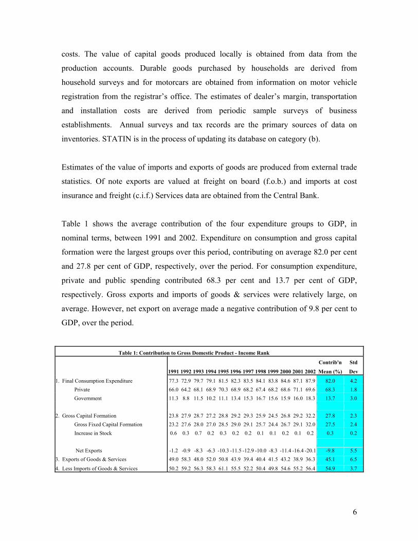
Table 1 shows the average contribution of the four expenditure groups to GDP, in

nominal terms, between 1991 and 2002. Expenditure on consumption and gross capital

formation were the largest groups over this period, contributing on average 82.0 per cent

and 27.8 per cent of GDP, respectively, over the period. For consumption expenditure,

private and public spending contributed 68.3 per cent and 13.7 per cent of GDP,

respectively. Gross exports and imports of goods & services were relatively large, on

average. However, net export on average made a negative contribution of 9.8 per cent to

GDP, over the period.

Table 1: Contribution to Gross Domestic Product - Income Rank

Contrib'n Std

1991 1992 1993 1994 1995 1996 1997 1998 1999 2000 2001 2002 Mean (%) Dev

1. Final Consumption Expenditure 77.3 72.9 79.7 79.1 81.5 82.3 83.5 84.1 83.8 84.6 87.1 87.9 82.0 4.2 Private 66.0 64.2 68.1 68.9 70.3 68.9 68.2 67.4 68.2 68.6 71.1 69.6 68.3 1.8 Government 11.3 8.8 11.5 10.2 11.1 13.4 15.3 16.7 15.6 15.9 16.0 18.3 13.7 3.0 2. Gross Capital Formation 23.8 27.9 28.7 27.2 28.8 29.2 29.3 25.9 24.5 26.8 29.2 32.2 27.8 2.3 Gross Fixed Capital Formation 23.2 27.6 28.0 27.0 28.5 29.0 29.1 25.7 24.4 26.7 29.1 32.0 27.5 2.4 Increase in Stock 0.6 0.3 0.7 0.2 0.3 0.2 0.2 0.1 0.1 0.2 0.1 0.2 0.3 0.2 Net Exports -1.2 -0.9 -8.3 -6.3 -10.3 -11.5 -12.9 -10.0 -8.3 -11.4 -16.4 -20.1 -9.8 5.5 3. Exports of Goods & Services 49.0 58.3 48.0 52.0 50.8 43.9 39.4 40.4 41.5 43.2 38.9 36.3 45.1 6.5

4. Less Imports of Goods & Services 50.2 59.2 56.3 58.3 61.1 55.5 52.2 50.4 49.8 54.6 55.2 56.4 54.9 3.7

6

3.0 Literature Review

Attempts to solve the problem of low frequency or missing GDP (and other) data have a

long history. Researchers have, for good reasons, opted to generate quarterly observations

(more formally referred to as temporal disaggregation) through a process called

“Benchmarking” – combining a series of high frequency data with a series of less

frequent data. The main problem in benchmarking arises when the two series show

inconsistent movements, and the less frequent data is considered the more reliable.

Benchmarking is generally done retrospectively as annual benchmark data are available

some time after quarterly data. This procedure also has a forward-looking element in that

the relationship between benchmark and indicator data (benchmark: indicator ratio) can

be extrapolated forward to improve quarterly estimates for the most recent periods for

which benchmark data are not yet available.

There are two main approaches to benchmarking time series data, namely a purely

numerical approach and a statistical approach. The numerical approach differs from the

statistical approach in that simulated data are not assumed to follow a specified a

statistical time series model. The numerical approach encompasses the family of least

squares minimization methods proposed by Denton (1971), Helfsand et al (1977), Bassie

(1958) and the method proposed by Ginsburgh (1973). Lisman and Sandee (1964) also

proposed a set of weights that could be used to generate quarterly GDP estimates from

annual data. The statistical modelling approach encompasses ARIMA model based

methods proposed by Hillmer and Trabelis (1987) and State space models proposed by

Durbin and Quenneville (1997) and implemented by Bernanke, Gertler and Watson

(1997) to interpolate real GDP in the United States of America. In addition, Chow and

Lin (1971) proposed a multivariate general least squares regression approach for

interpolation, distribution, and extrapolation of time series. While not being a

benchmarking method in a strict sense, the Chow-Lin method is related to the statistical

approach.

Lanning (1986) also conceptualised a third approach in which missing data is estimated

simultaneously with model parameters. He then sought to compare the model results with

7

the traditional benchmarking approach in which the missing data is first interpolated and

then used to estimate the model. He however found that the estimates of the model

parameters from the simultaneous approach have a larger variance and are less reliable

than the model parameters estimated with complete data in the second stage.

There has been some interest in the Caribbean in producing quarterly GDP estimates in

the absence of official statistics. Allen (2002), generated supply side based estimates of

quarterly GDP by employing the Denton Least Squares estimates, supported by other

numerical measures such as the Lisman & Sandee (1986) method. A statistical approach

was employed, on a somewhat more aggregated model, to produce a longer time series

but this was fairly rudimentary in nature. Nicholls, Coker and Forde (1995) also

attempted to generate quarterly GDP for Trinidad and Tobago in the framework of the

now outdated Lisman Sandee (1986) method. They found that these estimates were not

robust when compared with the official statistics, and proposed to advance the

investigation by reviewing the relative merit of the Chow & Lin (1971) method.

This paper goes beyond these two attempts to evaluate the most robust statistical method

available to date against the most widely used numerical method. In the remainder of this

section, we set out the broad framework the Denton Least Squares methods and the State

Space Approach – the best representatives of the two broad classes of benchmarking

techniques.

3.1. Denton Least Squares Estimates

The Denton (1971) Least Squares formulation was designed to eliminate the “step

problem” that arises when related series, with imperfect coverage, are used to interpolate

low frequency GDP data. The step problem occurs when the Benchmark to Indicator (BI)

ratio changes dramatically from year, given that the indicator or related series that is used

in the distribution process grows at different rate from the benchmark. Step problems are

most evident in simple pro-rata distribution techniques which is implemented as follows:

=

∑q qqq I

AIX

β

βββ ,.,,

8

Xq,ß is the level of the quarterly national accounts estimate for quarter q of year ß. Iq, ß is

the level of the indicator in quarter q of year ß, and Aß is the level of the annual data for

year ß. The expression

∑q qIA

β

β

,is the annual BI ratio. With pro rata distribution, there

will be a distinct jump in adjacent Xq,ß’s when Iq, ß and Aß grows at different rates, such

that the compensating adjustment in quarterly estimates from one distinct year to the next

will be put into the first quarter of each year, while other quarterly growth rates are left

unchanged. The significance of the step problem depends on the size of the variation in

the annual BI ratio.

To maintain simplicity, we outline only the basic version of the Denton Least square

method (the Proportional Denton Technique or PDT). This method involves solving the

following optimisation problems:

( )2

2 1

1min

41 ......... ∑= −

−

−

T

t t

t

t

tT I

XIX

XXX β

under the restriction that, for the flow series,

{ }β...........1,2

∈=∑=

yAX y

T

tt

4

where t is time5. Intuitively, the PDT implicitly constructs from the annual observed BI

ratios a time series of quarterly BI ratios that is as smooth as possible. Enhancements to

the PDT improve the ability of the technique to extrapolate based on available indicators

when there are no available annual benchmarks.

3.2 State Space Models and the Kalman Filter

State space models (SSMs) have been applied in the econometric literature to model

unobserved variables, such as expectations, measurement errors, missing observation and

4 The sum of the quarters should be equal to the independent annual estimate for each benchmark year. 5 (t=4y-3) is equal to the first quarter of year y, and t=4y the fourth quarter of year y. Similarly, t=1 is equal to the first quarter of year 1

9

unobserved components (cycles and trends). A thorough survey of the application of

SSMs in econometrics can be found in Hamilton (1994) and Harvey (1989).

The idea behind a state-space representation is to capture the dynamics of an observed

(nx1) vector “y”, in terms of a possibly unobserved (rx1) “state” vector ξt, known as the

observation equation for the system:

tttt wHxAy +′+′= ξ

Here yt is an (n x 1) vector of variables that is observed at date t, H′ is an (n x r) matrix of

coefficients, and wt is an (n x 1) vector that could be described as measurement error; wt

is assumed to be i.i.d N(0,R) and independent of ξ1 and vt for (τ = 1,2,...). Equation (1.6)

also includes xt, a (k x 1) vector of observed variables that are exogenous or

predetermined and which enter the expression through the (n x k) matrix of coefficients

A′.

The dynamics of ξt are assumed to follow the following autoregressive process (typically

called the state equation):

11 ++ += ttt vFξξ

The state and observation equations constitute a linear state-space representation for the

dynamic behaviour of y. The framework can be further generalized to allow for time-

varying coefficient matrices, non-normal disturbances and non-linear dynamics.

There are two advantages in representing a dynamic system in state space form. Firstly,

the state space model allows unobserved variables (state variables) to be incorporated

into and estimated along with the observable model. Secondly, these models can be

analysed using a Kalman (1960) filter6.

6 The Kalman filter algorithm has also been utilised to compute exact, finite sample forecasts for Gaussian ARMA models, multivariate ARMA models, multiple indicators & multiple causes (MIMIC), Markov Switching models and time varying coefficient models.

10

The multivariate Kalman filter is an algorithm for calculating the sequence T

ttt

11

=+

∧

ξ and

{ }T

tttP11 =+ , where tt 1+

∧

ξ denotes the optimal forecast of 1+tξ , based on observations of

( )ttt xxxxyyyy ,,....,,,,...,, 1211210 −− t xy ,, 0 , and ttP 1+ denotes the mean squared error

(MSE) of this forecast. The filter is implemented by iterating expressions7 determining

tt 1+

∧

ξ and ttP 1+ for t=1,2,………T.

3.3 Methodology

In this particular application, yt in (2) is an expenditure category, while xt is the indicator

series related to that particular component. The equations for this system are as follows:

111 +++ +′+= tttt RvxCFξξ (1)

(2) ttttt hxay ξ⋅′+′=

Following Cuche and Hess (1999), yt is given in each quarter as follows: y1 = 0, y2 = 0,

y3 = 0, y4 = annual figure. When these annual observations are stored in one column, the

‘zero’ observations are not included, resulting in a reduced vector of size [ ]14 ×T

. Time-

invariant coefficients are assumed for the matrices, F, C′ and R.

The observation equation embodies the constraint that the sum of four quarterly

observations within a year equals the annual observed GDP. In this regard, no error term

is specified for the observation equation, so that the Kalman filter generates exact values

of the coefficients vector a′t and h′t to ensure the summation condition holds.

4.0 Identification of Related Series

To facilitate the interpolation of the components of quarterly GDP by expenditure, sets of

quarterly indicators were identified and assessed for their accuracy and timeliness. The

7 See Hamilton (1999) for a full discussion of the Kalman filter.

11

main criterion for the accuracy of the indicators is the extent to which they are successful

in mimicking the annual movements in the benchmark series. The timeliness of the

quarterly source data also has important implications for how early sufficiently reliable

quarterly estimates can be prepared, after the end date for a reference period. These

indicators were also carefully selected with an eye to the set of indicators used by

STATIN in estimating each category annually. Where more than one indicator was

identified for a particular expenditure group, a weighted index was created. These

weights were selected from an algorithm that generated the highest correlation between

the changes in the combined indicator with the GDP.

4.1 Final Consumption Expenditure

Final consumption expenditure consists of private and public spending. In regard to

private consumption spending, the candidate indicators included general consumption tax

(GCT) & special consumption tax (SCT) receipts from local transactions, total imports of

goods & services and a composite production index reflecting quarterly value added from

the agriculture, manufacturing, electricity & water and transport, storage &

communication sectors. The latter indicator is consistent with STATIN’s method of

estimating consumption of locally produced commodity and is premised on the

assumption that the output of these sectors is purchased by Jamaican consumers. Also

consistent with the commodity flow approach, we combine the tax data with the series on

imports, to capture the broad disaggregation of household spending on domestically

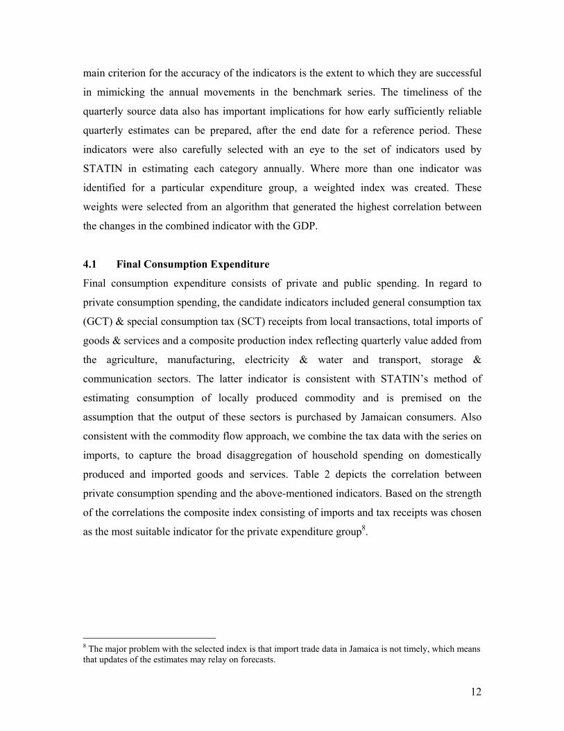
produced and imported goods and services. Table 2 depicts the correlation between

private consumption spending and the above-mentioned indicators. Based on the strength

of the correlations the composite index consisting of imports and tax receipts was chosen

as the most suitable indicator for the private expenditure group8.

8 The major problem with the selected index is that import trade data in Jamaica is not timely, which means that updates of the estimates may relay on forecasts.

12

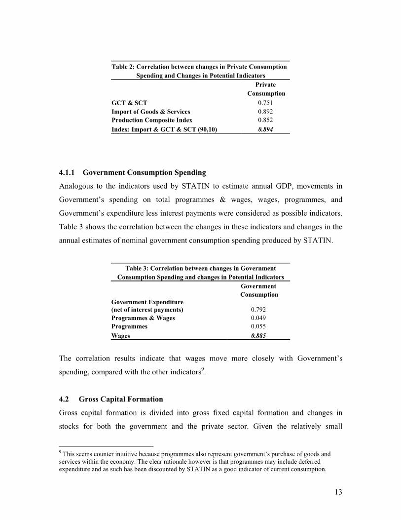
Table 2: Correlation between changes in Private Consumption Spending and Changes in Potential Indicators Private Consumption GCT & SCT 0.751 Import of Goods & Services 0.892 Production Composite Index 0.852 Index: Import & GCT & SCT (90,10) 0.894

4.1.1 Government Consumption Spending

Analogous to the indicators used by STATIN to estimate annual GDP, movements in

Government’s spending on total programmes & wages, wages, programmes, and

Government’s expenditure less interest payments were considered as possible indicators.

Table 3 shows the correlation between the changes in these indicators and changes in the

annual estimates of nominal government consumption spending produced by STATIN.

Table 3: Correlation between changes in Government Consumption Spending and changes in Potential Indicators

Government Consumption Government Expenditure (net of interest payments) 0.792 Programmes & Wages 0.049 Programmes 0.055 Wages 0.885

The correlation results indicate that wages move more closely with Government’s

spending, compared with the other indicators9.

4.2 Gross Capital Formation

Gross capital formation is divided into gross fixed capital formation and changes in

stocks for both the government and the private sector. Given the relatively small

9 This seems counter intuitive because programmes also represent government’s purchase of goods and services within the economy. The clear rationale however is that programmes may include deferred expenditure and as such has been discounted by STATIN as a good indicator of current consumption.

13

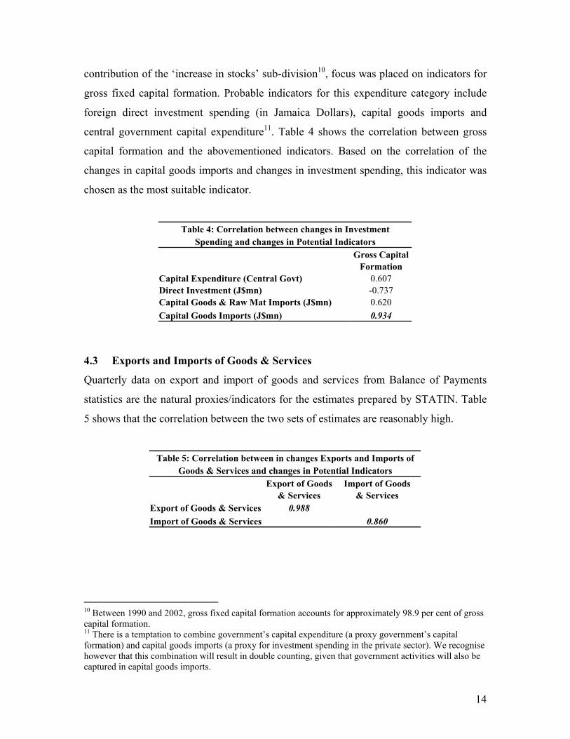
contribution of the ‘increase in stocks’ sub-division10, focus was placed on indicators for

gross fixed capital formation. Probable indicators for this expenditure category include

foreign direct investment spending (in Jamaica Dollars), capital goods imports and

central government capital expenditure11. Table 4 shows the correlation between gross

capital formation and the abovementioned indicators. Based on the correlation of the

changes in capital goods imports and changes in investment spending, this indicator was

chosen as the most suitable indicator.

Table 4: Correlation between changes in Investment Spending and changes in Potential Indicators

Gross Capital Formation Capital Expenditure (Central Govt) 0.607 Direct Investment (J$mn) -0.737 Capital Goods & Raw Mat Imports (J$mn) 0.620 Capital Goods Imports (J$mn) 0.934

4.3 Exports and Imports of Goods & Services

Quarterly data on export and import of goods and services from Balance of Payments

statistics are the natural proxies/indicators for the estimates prepared by STATIN. Table

5 shows that the correlation between the two sets of estimates are reasonably high.

Table 5: Correlation between in changes Exports and Imports of Goods & Services and changes in Potential Indicators

Export of Goods Import of Goods & Services & Services Export of Goods & Services 0.988 Import of Goods & Services 0.860

10 Between 1990 and 2002, gross fixed capital formation accounts for approximately 98.9 per cent of gross capital formation. 11 There is a temptation to combine government’s capital expenditure (a proxy government’s capital formation) and capital goods imports (a proxy for investment spending in the private sector). We recognise however that this combination will result in double counting, given that government activities will also be captured in capital goods imports.

14

4.4 Deflators

The aim of this paper is to generate quarterly estimates of real expenditure. STATIN,

however, only produces nominal GDP by the expenditure method. In this context, it is

necessary to identify appropriate deflators to convert the quarterly nominal estimates to

constant price estimates. This represented the main data challenge for the paper, given

that there are no benchmarks available to test the adequacy of the deflators. To partly

offset this deficiency, we also opted to identify the best proxy deflators for the annual

estimates produced by STATIN. The deflators for the indicators were, in some cases,

different from the ones employed for the annual estimates. This section discusses the

choices of the deflators for both the related series and the benchmarks.

Both private and government consumption spending were deflated using an appropriate

average consumer price index (CPI). The indicators were deflated using an index

generated from a series of three-month average CPI. For gross capital formation, we

identified the implicit deflator for the construction sector, generated from the production

accounts, as an appropriate deflator for the annual estimates prepared by STATIN. For

the quarterly indicators, the index of housing and other housing expenses sub-index

within the CPI was employed. Annual import and export price indices are available from

STATIN, which, when augmented by an appropriate proxy for price inflation in

Jamaica’s import and export of services, were considered the best proxies for deflating

the annual nominal estimates. The development of quarterly deflators for the indicators

was however, produced by a fairly involved method12.

Jamaica’s imports are disaggregated into the standard end-use classification (consumer

goods, raw materials and capital goods). U.S. export price indices, taken from the Bureau

of Labour Statistics in the United States for similar categories of goods, were used as

proxies of Jamaica’s goods import prices. The U.S. export prices were used because the

U.S.A. is Jamaica’s principal trading partner, accounting for around 46 per cent of total

imports between 1998 and 2002. One exception was the fuel category for which the West

12 At the time of the development of this paper, STATIN had promised to provide the author with quarterly import volumes, which could be used to generate more appropriate deflators. We anticipate that the receipt of this data will improve the quality of the analysis.

15

Texas Intermediate index of crude oil price was used. A list of import categories and their

respective proxies are presented in the appendix, Table 1. To customise this index for

Jamaica, the weights of the commodities in the Jamaican import basket were applied to

the individual US indices.

For exports, implicit prices are readily available for selected major traditional and other

traditional exports, including bauxite, alumina, sugar and banana. Since tourism is

Jamaica’s main foreign exchange earner, outside of remittances, it was important to also

include this export service13. The travel sector accounts for the largest share of export

earnings followed by alumina, with both accounting for over 90.0 per cent of the value of

exports used in the index (see Table 2 in Appendix). In the case of exports, the same

deflators were employed in the conversion of both the annual STATIN estimates and the

quarterly indicators. Consistent with the supply side estimates, all the constant price

series were based in 1996.

Procedurally, the quarterly estimates of the items of expenditure were generated by

converting to 1996 prices, both the annual estimates from STATIN and the quarterly

indicators with the relevant deflators as discussed above. The constant price annual

benchmarks were then interpolated with the constant price indicators via both the DLSM

and SSM14.

Given the absence of constant price estimates by STATIN at the annual level, the

evaluation of the output from the DLSM and SSM was conducted from in two steps.

Firstly, we evaluated the relative presence of the “step problem” between the two sets of

estimates, using simulated quarterly BI ratios and looking for structural breaks in these

13 It is important to recognise that the use of implicit prices (ratio of export value to volume) for the export data creates potential problems. Variations in these prices may reflect changes in the quality of the product from month to month and therefore the price received but not changes in the underlying price of the product measured at a consistent quality. Moreover, the proxy used for tourism prices represents the average daily expenditure per tourist and not his actual expenditure per unit of tourism services and may therefore reflect changes in the quantity of tourism services consumed as well as price changes. 14 We recognise that it would have been equally possible to interpolate the nominal annual data and then deflate the quarterly estimates using the identified deflators, appropriately adjusted for their relationship with the annual proxies.

16

ratios in the first quarter of each year. Secondly, we compared the aggregated quarterly

GDP derived from the two methods with the quarterly estimates currently produced by

STATIN over common samples. The idea is that the two methods (supply side estimates

and demand side estimates) should in theory generate the same estimates for a particular

economy. Assuming that the quarterly estimates produced by STATIN are more reliable,

the goodness of fit of the respective methods with respect to these estimates should

provide a perspective on which one is relatively sounder. This exercise involves the

evaluation of estimated growth rates and Theil U statistics from the two competing

models.

5.0 Results and Analysis

The interpolation result from the DLSM is found in Appendix B and that from the SSM is

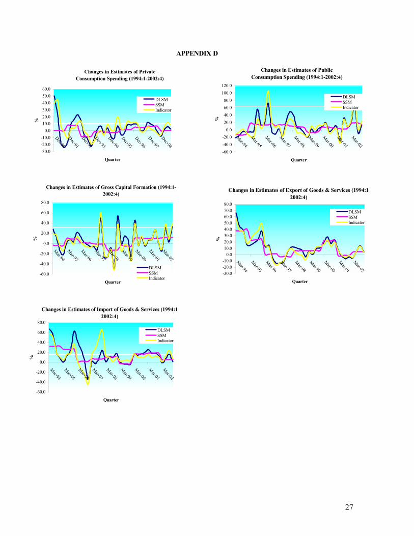
found in Appendix C. A comparison of the year over year changes in the quarterly real

estimates derived from the DLSM and the SSM are found in Appendix D. The most

significant observation is that the estimates from the DSLM more closely track the

changes in the indicator, than the estimates from the SSM, because the state space model

smoothes out the volatility in the indicators.

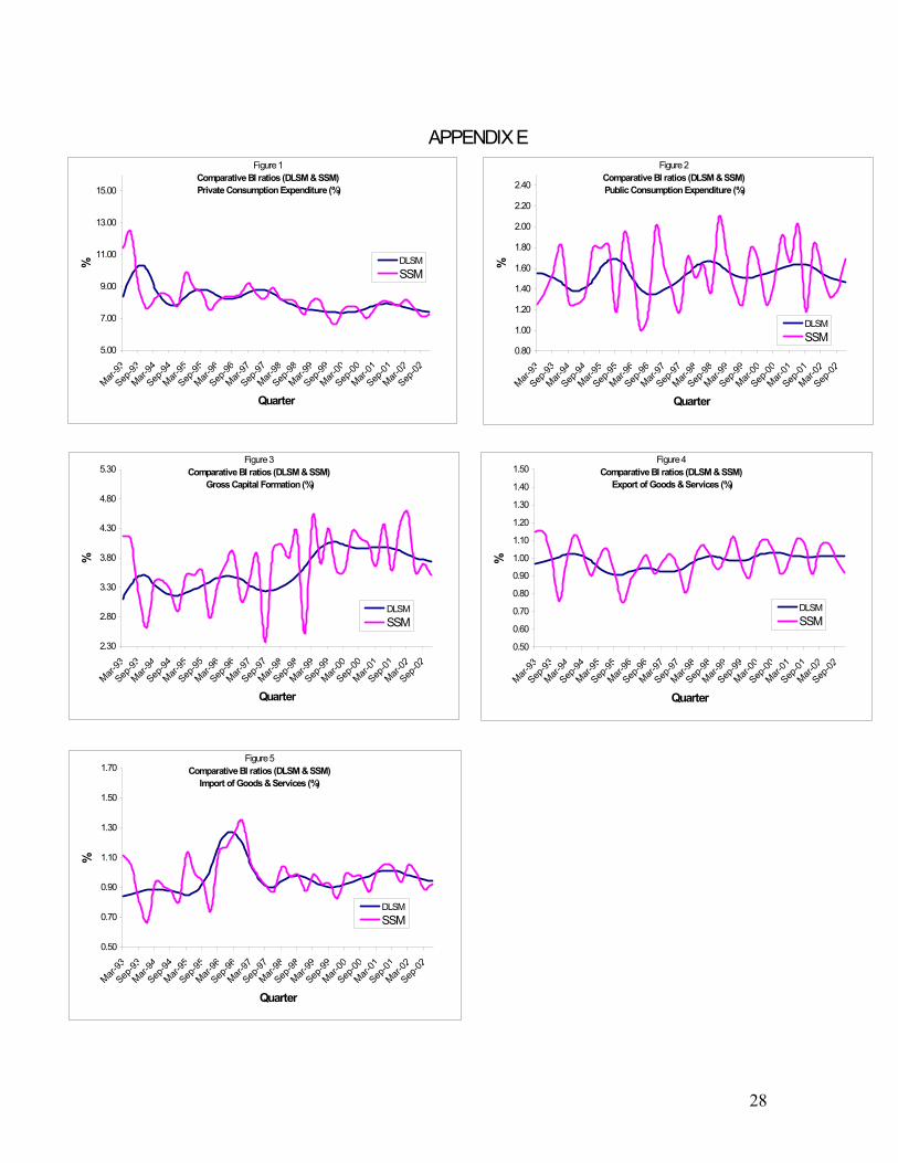
The SSM also appeared to be less consistent compared with the DLSM, when account is

taken of the BI ratios. Appendix E presents the relative plots of simulated quarterly BI

ratios for the various components of spending. The simulated BI ratios for the SSM are

more volatile than those for the DLSM, in particular, the ratios for public consumption

and gross capital formation. Table 5 in the appendix confirms this as the relative presence

of the step problem is more pronounced in the SSM ratios.

Despite the apparent shortcomings of the SSMs in respect of conformity with the

indicators and in terms of the step problem, the aggregated quarterly GDP generated from

this method has better in sample forecasting properties. Table 6 in the appendix

highlights that the SSM has lower mean squared error, root mean square error and Theil

U statistics, relative to the DLSM. A decomposition of the Theil statistics into its

constituent proportions reveals that the main source of the poor fit of the DLSM is the

17

variance proportion. The SSM, conversely, has a larger covariance proportion, suggesting

that a greater proportion of the error generated within sample is unsystematic. Consistent

with the higher co-movement of the DLSM estimates with the indicator and the relatively

lower level of step problem, the bias proportion for this model is lower than the SSM.

This fairly startling discovery is indicative of a shortcoming of the DLSM method. When

the indicator is volatile, the DLSM will project this volatility into the estimates. We find

that even though the summation condition holds and the step problem is minimised, the

goodness of fit of this class of model tends to suffer under these conditions. The SSM,

however, will tend to smooth the volatility in the estimates and therefore improve the

goodness of fit. The latter interpolation is to be preferred, as economic agents will more

engage in consumption smoothing than suggested by the volatility in the indicators.

5.1 Stylised Facts: Quarterly Real Expenditure Components

The objective of this section is to determine and evaluate the basic time series patterns

underlying the quarterly real estimates derived from the SSM. The data for each category

of expenditure was decomposed into their trend, seasonal and cyclical components (see

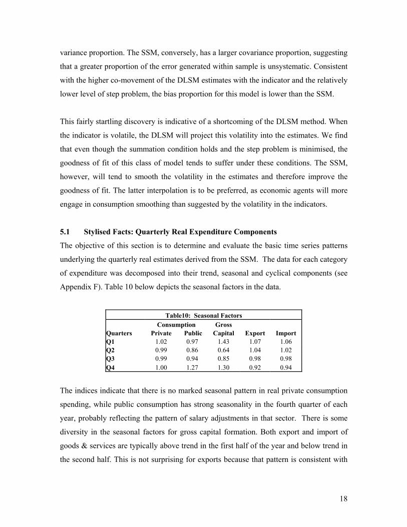
Appendix F). Table 10 below depicts the seasonal factors in the data.

Table10: Seasonal Factors Consumption Gross Quarters Private Public Capital Export Import Q1 1.02 0.97 1.43 1.07 1.06 Q2 0.99 0.86 0.64 1.04 1.02 Q3 0.99 0.94 0.85 0.98 0.98 Q4 1.00 1.27 1.30 0.92 0.94

The indices indicate that there is no marked seasonal pattern in real private consumption

spending, while public consumption has strong seasonality in the fourth quarter of each

year, probably reflecting the pattern of salary adjustments in that sector. There is some

diversity in the seasonal factors for gross capital formation. Both export and import of

goods & services are typically above trend in the first half of the year and below trend in

the second half. This is not surprising for exports because that pattern is consistent with

18

the pattern of tourist arrivals to the Island. The expectation for imports, however, was that

there would have been relatively higher volumes in advance of the Christmas season.

The cyclical component (Appendix E) indicates that real consumption expenditure grew

strongly between the beginning of 1993 and end–1995. There was sustained recession in

this category of spending between 1996 and 2000, followed by a gradual recovery since

2001. There is no clearly discernible relationship between this cycle and real interest

rates. What is noticeable however is that real consumption expenditure fell off in early

1996 when real rates were dramatically increased, and started to recover in a context of a

sustained reduction in real rates after 1998. The investment and import cycles are not

markedly different from private consumption and, as expected, investment does not

appear to be explained by real interest rates. The data indicates that there has been a

sustained growth in gross capital formation since the beginning of 2000, probably

associated with the accelerated programme of public sector asset divestment. Public

consumption has a regular pattern that appears to coincide with the election cycle.

6.0 Conclusion

In the last few years, the interest in short-term national accounts statistics has increased

considerably. The availability of suitable statistics to depict an image of the economy

with a short delay and in a reliable way has become one of the main challenges for

Jamaica. More importantly, there is the need for higher frequency data as economic

processes and activities are enacted rapidly over time. In these regard the above work

provides a valuable contribution in estimating and updating a quarterly expenditure series

for Jamaica. Of note, some of the indicators, in particular, gross capital formation, can be

enhanced.

Based on the results from the two competing models, the Denton’s Least Square Model

better projects the changes in the indicators into the quarterly estimates, but this will, in

the context of a volatile indicator, lead to questionable in sample properties of the

estimates.

19

The paper has, in the main, addressed some of the main methodological issues in

generating quarterly estimates of expenditure. Further refinements are possible in terms

of improving the quality of the indicators and in relation to extrapolating the items of

expenditure beyond the available data.

20

Bibliography Allen, Courtney, 2002, “Estimating Quarterly Gross Domestic Product for Jamaica”,

Research Department, Bank of Jamaica. Bank of Jamaica, “National Income Workbook: Jamaica System of National Accounts –

Present System”, Bank of Jamaica. Bassi, V., 1958, “Appendix A,” Economic Forecasting, ed. By V.L. Bassi (New York:

McGraw-Hill) Bernanke B., Gertler, M. and M. Watson, 1997, “Systematic Monetary Policy and the

Effects of Oil Shocks”, Brookings Papers on Economic Activity, (1): 91-157. Central Statistical Office, 1968, “National Accounts Statistics: Sources and Methods”,

Her Majesty’s Stationary Office. Chow, G. and A. Lin, 1971, “Best Linear Unbiased Interpolation, Distribution and

Extrapolation of Time Series by Related Series”, The Review of Economics and Statistics, 53 (4): 372 – 375.

Chow, G. and A. Lin, 1976, “Best Linear Unbiased Estimation of Missing Observation in

an Economic Time Series”, Journal of the American Standard Association, 71 (355), 719 – 721.

Cuche, N. and M. Hess, 1999, “Estimating Monthly GDP in a General Kalman Filter

Framework: Evidence from Switzerland”, Working Paper, Swiss National Bank, Study Center Gerzensee.

Denton, Frank, 1971, “Adjustments of monthly or Quarterly Series to Annual Totals; An

Approach Based on Quadratic Minimization”, Journal of the American Statistical Associations, 66 (333): 99 – 102.

Durbin, J. and B. Quenneville, 1997, “Benchmarking by State Space Models,”

International Statistical Review, Vol. 65, No. 1, pp. 23-48. Fernandez, Roque, 1981, “A Methodology Note on the Estimation of Time Series”,

Journal of the American Statistical Association, 63 (3): 471-476. Ginsburgh, V.A., 1973, “A Further Note on the Derivation of Quarterly Figures

Consistent with Annual Data,” Applied Statistics, Vol. 22, No. 3, pp. 368-74. Hamilton, James, 1994a, “Times Series Analysis”, Princeton University Press.

21

Hamilton, James, 1994, “State Space Models” in Robert Engle and Daniel McFadden, eds., Handbook of Econometrics, Volume 4. Amsterdam: Elsevier.

Harvey, Andrew, 1989, “Forecasting, Structural Series and the Kalman Filter”,

Cambridge University Press. Helfand, S., Monsour, N. and M. Trager, 1977, “Historical Revision of Current Business

Survey Estimates,” Proceedings of the Business and Economic Statistics Section, American Statistical Association, pp. 246-50.

Hillmer, S. and A. Trabelsi, 1987, “Benchmarking of Economic Time Series,” Journal of

the American Statistical Association, Vol. 82 (December), pp. 1064-71. Lanning, Steven, 1986, “Missing Observations: A Simulation Approach Versus

Interpolation by Related Series”, Journal of Economic and Social Measurement, 14 (1): 155 – 163.

Lisman, J. and J. Sandee, 1964, “Derivation of Quarterly Figures from Annual Data”,

Journal of the Royal Statistical Society (Series C), 13, 87-90 Liu, H. and S. Hall, 2001, “Creating High Frequency National Accounts with State Space

Modelling: A Monte Carlo Experiment”, Journal of Forecasting, vol. 20, pp. 441-49.

Rose, Dexter, “A Framework for Revising the National Accounts of Jamaica”,

Department of Statistics, Jamaica. The Statistical Institute of Jamaica, (Various Years) “National Income and Product”. International Monetary Fund, General Data Dissemination System Site – Jamaica.

22

APPENDICES

23

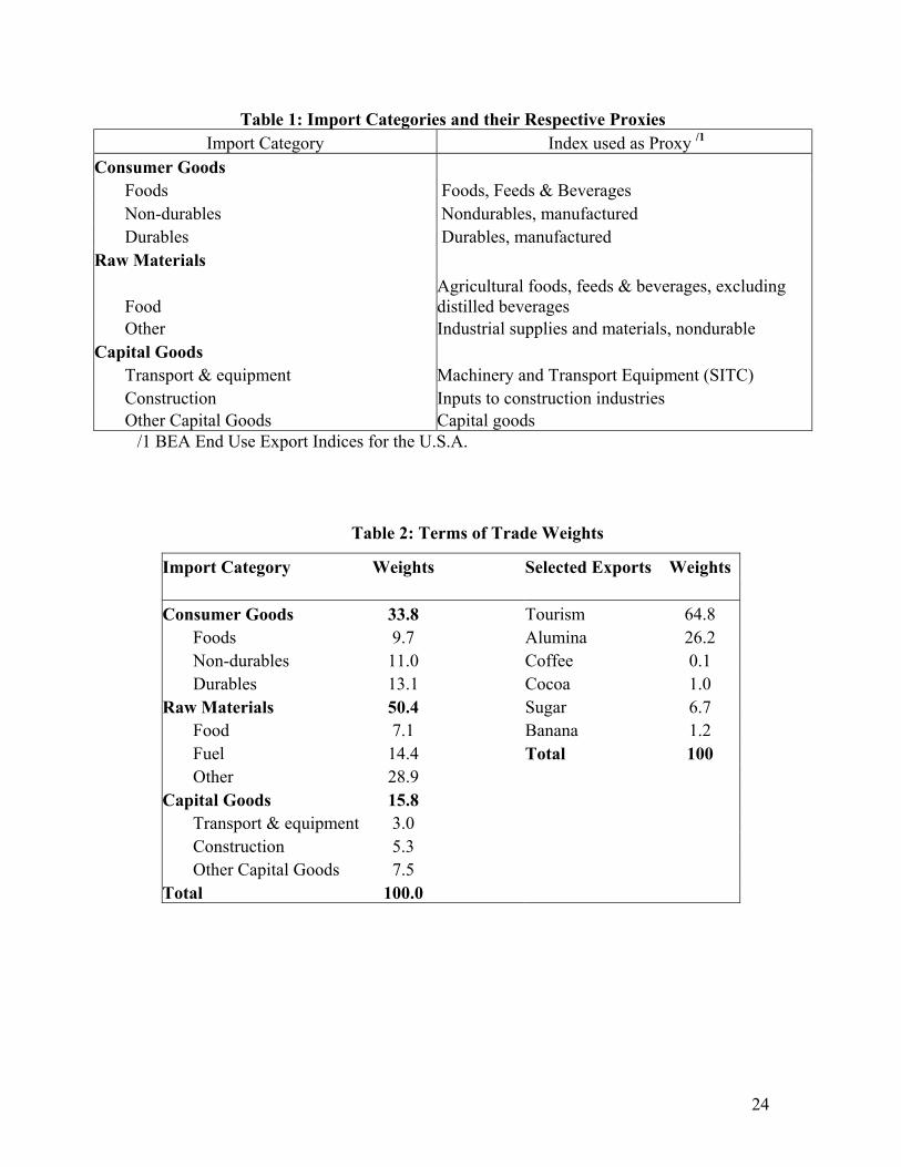
Table 1: Import Categories and their Respective Proxies Import Category Index used as Proxy /1

Consumer Goods Foods Foods, Feeds & Beverages Non-durables Nondurables, manufactured Durables Durables, manufactured

Raw Materials

Food Agricultural foods, feeds & beverages, excluding distilled beverages

Other Industrial supplies and materials, nondurable Capital Goods

Transport & equipment Machinery and Transport Equipment (SITC) Construction Inputs to construction industries Other Capital Goods Capital goods /1 BEA End Use Export Indices for the U.S.A.

Table 2: Terms of Trade Weights

Import Category Weights Selected Exports Weights Consumer Goods 33.8 Tourism 64.8

Foods 9.7 Alumina 26.2 Non-durables 11.0 Coffee 0.1 Durables 13.1 Cocoa 1.0

Raw Materials 50.4 Sugar 6.7 Food 7.1 Banana 1.2 Fuel 14.4 Total 100 Other 28.9

Capital Goods 15.8 Transport & equipment 3.0 Construction 5.3 Other Capital Goods 7.5

Total 100.0

24

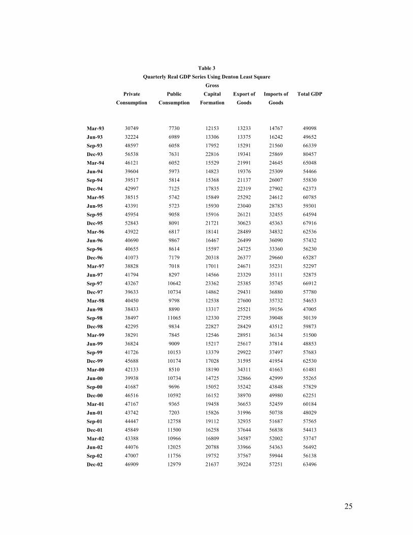
Table 3 Quarterly Real GDP Series Using Denton Least Square

Gross Private Public Capital Export of Imports of Total GDP Consumption Consumption Formation Goods Goods Mar-93 30749 7730 12153 13233 14767 49098 Jun-93 32224 6989 13306 13375 16242 49652 Sep-93 48597 6058 17952 15291 21560 66339 Dec-93 56538 7631 22816 19341 25869 80457 Mar-94 46121 6052 15529 21991 24645 65048 Jun-94 39604 5973 14823 19376 25309 54466 Sep-94 39517 5814 15368 21137 26007 55830 Dec-94 42997 7125 17835 22319 27902 62373 Mar-95 38515 5742 15849 25292 24612 60785 Jun-95 43391 5723 15930 23040 28783 59301 Sep-95 45954 9058 15916 26121 32455 64594 Dec-95 52843 8091 21721 30623 45363 67916 Mar-96 43922 6817 18141 28489 34832 62536 Jun-96 40690 9867 16467 26499 36090 57432 Sep-96 40655 8614 15597 24725 33360 56230 Dec-96 41073 7179 20318 26377 29660 65287 Mar-97 38828 7018 17011 24671 35231 52297 Jun-97 41794 8297 14566 23329 35111 52875 Sep-97 43267 10642 23362 25385 35745 66912 Dec-97 39633 10734 14862 29431 36880 57780 Mar-98 40450 9798 12538 27600 35732 54653 Jun-98 38433 8890 13317 25521 39156 47005 Sep-98 38497 11065 12330 27295 39048 50139 Dec-98 42295 9834 22827 28429 43512 59873 Mar-99 38291 7845 12546 28951 36134 51500 Jun-99 36824 9009 15217 25617 37814 48853 Sep-99 41726 10153 13379 29922 37497 57683 Dec-99 45688 10174 17028 31595 41954 62530 Mar-00 42133 8510 18190 34311 41663 61481 Jun-00 39938 10734 14725 32866 42999 55265 Sep-00 41687 9696 15052 35242 43848 57829 Dec-00 46516 10592 16152 38970 49980 62251 Mar-01 47167 9365 19458 36653 52459 60184 Jun-01 43742 7203 15826 31996 50738 48029 Sep-01 44447 12758 19112 32935 51687 57565 Dec-01 45849 11500 16258 37644 56838 54413 Mar-02 43388 10966 16809 34587 52002 53747 Jun-02 44076 12025 20788 33966 54363 56492 Sep-02 47007 11756 19752 37567 59944 56138 Dec-02 46909 12979 21637 39224 57251 63496

25

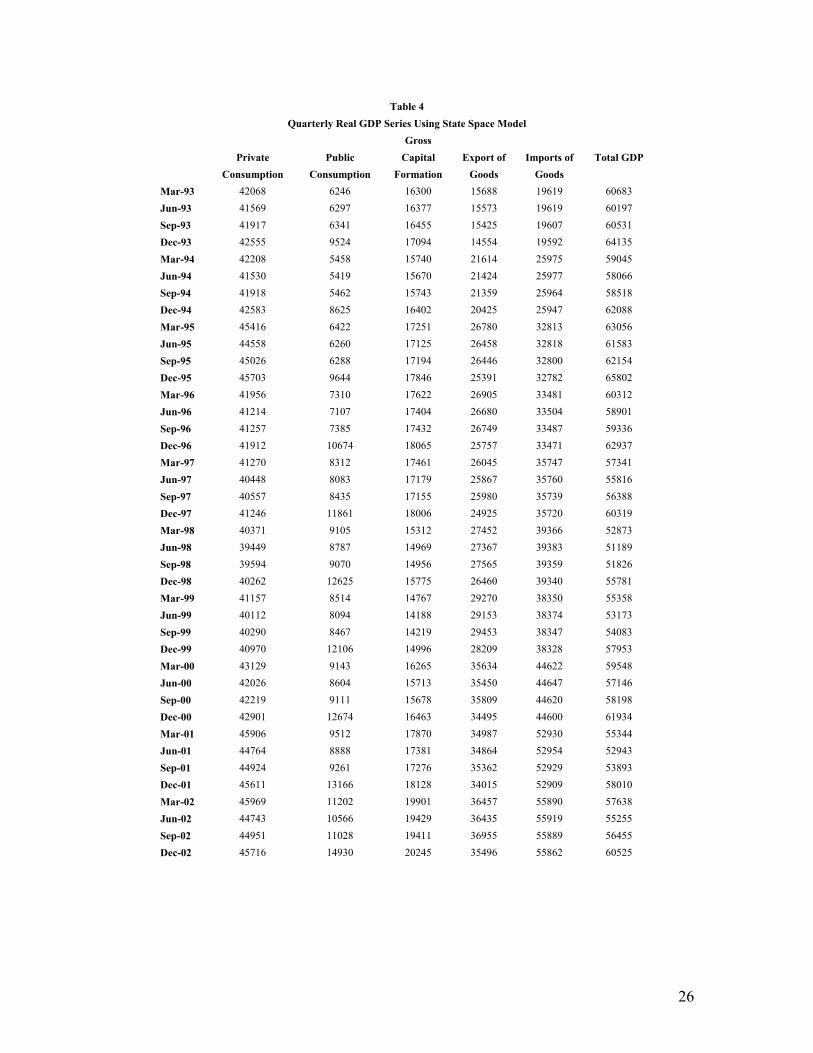
Table 4 Quarterly Real GDP Series Using State Space Model

Gross Private Public Capital Export of Imports of Total GDP Consumption Consumption Formation Goods Goods Mar-93 42068 6246 16300 15688 19619 60683 Jun-93 41569 6297 16377 15573 19619 60197 Sep-93 41917 6341 16455 15425 19607 60531 Dec-93 42555 9524 17094 14554 19592 64135 Mar-94 42208 5458 15740 21614 25975 59045 Jun-94 41530 5419 15670 21424 25977 58066 Sep-94 41918 5462 15743 21359 25964 58518 Dec-94 42583 8625 16402 20425 25947 62088 Mar-95 45416 6422 17251 26780 32813 63056 Jun-95 44558 6260 17125 26458 32818 61583 Sep-95 45026 6288 17194 26446 32800 62154 Dec-95 45703 9644 17846 25391 32782 65802 Mar-96 41956 7310 17622 26905 33481 60312 Jun-96 41214 7107 17404 26680 33504 58901 Sep-96 41257 7385 17432 26749 33487 59336 Dec-96 41912 10674 18065 25757 33471 62937 Mar-97 41270 8312 17461 26045 35747 57341 Jun-97 40448 8083 17179 25867 35760 55816 Sep-97 40557 8435 17155 25980 35739 56388 Dec-97 41246 11861 18006 24925 35720 60319 Mar-98 40371 9105 15312 27452 39366 52873 Jun-98 39449 8787 14969 27367 39383 51189 Sep-98 39594 9070 14956 27565 39359 51826 Dec-98 40262 12625 15775 26460 39340 55781 Mar-99 41157 8514 14767 29270 38350 55358 Jun-99 40112 8094 14188 29153 38374 53173 Sep-99 40290 8467 14219 29453 38347 54083 Dec-99 40970 12106 14996 28209 38328 57953 Mar-00 43129 9143 16265 35634 44622 59548 Jun-00 42026 8604 15713 35450 44647 57146 Sep-00 42219 9111 15678 35809 44620 58198 Dec-00 42901 12674 16463 34495 44600 61934 Mar-01 45906 9512 17870 34987 52930 55344 Jun-01 44764 8888 17381 34864 52954 52943 Sep-01 44924 9261 17276 35362 52929 53893 Dec-01 45611 13166 18128 34015 52909 58010 Mar-02 45969 11202 19901 36457 55890 57638 Jun-02 44743 10566 19429 36435 55919 55255 Sep-02 44951 11028 19411 36955 55889 56455 Dec-02 45716 14930 20245 35496 55862 60525

26

APPENDIX D

Changes in Estimates of Private Consumption Spending (1994:1-2002:4)

-30.0-20.0-10.0

0.010.020.030.040.050.060.0

Dec-90Dec-91Dec-92Dec-93Dec-94Dec-95Dec-96Dec-97Dec-98

Quarter

%

DLSMSSMIndicator

Changes in Estimates of Public Consumption Spending (1994:1-2002:4)

-60.0-40.0-20.0

0.020.040.060.080.0

100.0120.0

Mar-94

Mar-95

Mar-96

Mar-97

Mar-98

Mar-99

Mar-00

Mar-01

Mar-02

Quarter

%

DLSMSSMIndicator

Changes in Estimates of Gross Capital Formation (1994:1-2002:4)

-60.0

-40.0

-20.0

0.0

20.0

40.0

60.0

80.0

Mar-94

Mar-95

Mar-96

Mar-97

Mar-98

Mar-99

Mar-00

Mar-01

Mar-02

Quarter

%

DLSMSSMIndicator

Changes in Estimates of Export of Goods & Services (1994:1-2002:4)

-30.0-20.0-10.0

0.010.020.030.040.050.060.070.080.0

Mar-94

Mar-95

Mar-96

Mar-97

Mar-98

Mar-99

Mar-00

Mar-01

Mar-02

Quarter

%DLSMSSMIndicator

Changes in Estimates of Import of Goods & Services (1994:1-2002:4)

-60.0

-40.0

-20.0

0.0

20.0

40.0

60.0

80.0

Mar-94

Mar-95

Mar-96

Mar-97

Mar-98

Mar-99

Mar-00

Mar-01

Mar-02

Quarter

%

DLSMSSMIndicator

27

APPENDIX E

5.00

7.00

9.00

11.00

13.00

15.00

Mar-93

Sep-93

Mar-94

Sep-94

Mar-95

Sep-95

Mar-96

Sep-96

Mar-97

Sep-97

Mar-98

Sep-98

Mar-99

Sep-99

Mar-00

Sep-00

Mar-01

Sep-01

Mar-02

Sep-02

Quarter

% DLSMSSM

Figure 1Comparative BI ratios (DLSM & SSM) Private Consumption Expenditure (%)

0.80

1.00

1.20

1.40

1.60

1.80

2.00

2.20

2.40

Mar-93

Sep-93

Mar-94

Sep-94

Mar-95

Sep-95

Mar-96

Sep-96

Mar-97

Sep-97

Mar-98

Sep-98

Mar-99

Sep-99

Mar-00

Sep-00

Mar-01

Sep-01

Mar-02

Sep-02

Quarter

%

DLSMSSM

Figure 2Comparative BI ratios (DLSM & SSM) Public Consumption Expenditure (%)

2.30

2.80

3.30

3.80

4.30

4.80

5.30

Mar-93

Sep-93

Mar-94

Sep-94

Mar-95

Sep-95

Mar-96

Sep-96

Mar-97

Sep-97

Mar-98

Sep-98

Mar-99

Sep-99

Mar-00

Sep-00

Mar-01

Sep-01

Mar-02

Sep-02

Quarter

%

DLSMSSM

Figure 3Comparative BI ratios (DLSM & SSM)

Gross Capital Formation (%)

0.50

0.60

0.70

0.80

0.90

1.00

1.10

1.20

1.30

1.40

1.50

Mar-93

Sep-93

Mar-94

Sep-94

Mar-95

Sep-95

Mar-96

Sep-96

Mar-97

Sep-97

Mar-98

Sep-98

Mar-99

Sep-99

Mar-00

Sep-00

Mar-01

Sep-01

Mar-02

Sep-02

Quarter

%

DLSMSSM

Figure 4Comparative BI ratios (DLSM & SSM)

Export of Goods & Services (%)

0.50

0.70

0.90

1.10

1.30

1.50

1.70

Mar-93

Sep-93

Mar-94

Sep-94

Mar-95

Sep-95

Mar-96

Sep-96

Mar-97

Sep-97

Mar-98

Sep-98

Mar-99

Sep-99

Mar-00

Sep-00

Mar-01

Sep-01

Mar-02

Sep-02

Quarter

%

DLSMSSM

Figure 5Comparative BI ratios (DLSM & SSM)

Import of Goods & Services (%)

28

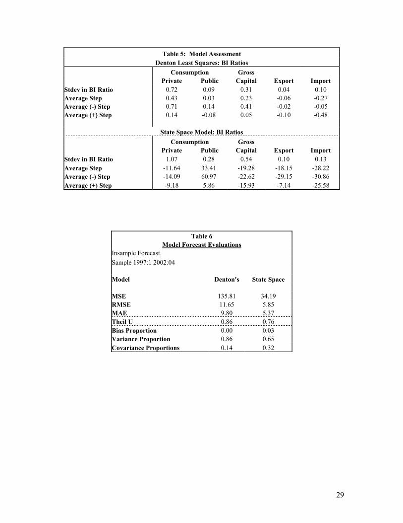
Table 5: Model Assessment Denton Least Squares: BI Ratios

Consumption Gross Private Public Capital Export Import Stdev in BI Ratio 0.72 0.09 0.31 0.04 0.10 Average Step 0.43 0.03 0.23 -0.06 -0.27 Average (-) Step 0.71 0.14 0.41 -0.02 -0.05 Average (+) Step 0.14 -0.08 0.05 -0.10 -0.48

State Space Model: BI Ratios Consumption Gross Private Public Capital Export Import Stdev in BI Ratio 1.07 0.28 0.54 0.10 0.13 Average Step -11.64 33.41 -19.28 -18.15 -28.22 Average (-) Step -14.09 60.97 -22.62 -29.15 -30.86 Average (+) Step -9.18 5.86 -15.93 -7.14 -25.58

Table 6 Model Forecast Evaluations

Insample Forecast. Sample 1997:1 2002:04 Model Denton's State Space MSE 135.81 34.19 RMSE 11.65 5.85 MAE 9.80 5.37 Theil U 0.86 0.76 Bias Proportion 0.00 0.03 Variance Proportion 0.86 0.65 Covariance Proportions 0.14 0.32

29

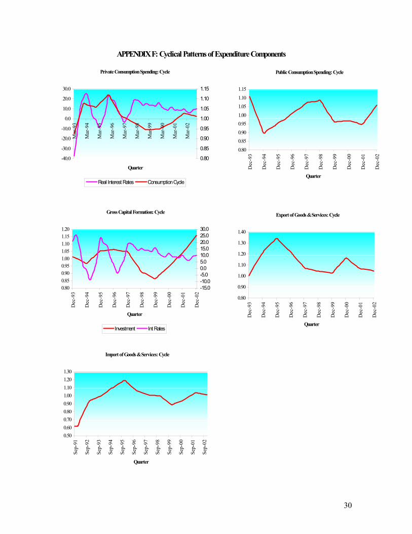
APPENDIX F: Cyclical Patterns of Expenditure Components

Private Consumption Spending: Cycle

-40.0

-30.0

-20.0

-10.0

0.0

10.0

20.0

30.0

Mar

-93

Mar

-94

Mar

-95

Mar

-96

Mar

-97

Mar

-98

Mar

-99

Mar

-00

Mar

-01

Mar

-02

Quarter

0.80

0.85

0.90

0.95

1.00

1.05

1.10

1.15

Real Interest Rates Consumption Cycle

Public Consumption Spending: Cycle

0.800.850.900.951.001.051.101.15

Dec

-93

Dec

-94

Dec

-95

Dec

-96

Dec

-97

Dec

-98

Dec

-99

Dec

-00

Dec

-01

Dec

-02

Quarter

Gross Capital Formation: Cycle

0.800.850.900.951.001.051.101.151.20

Dec

-93

Dec

-94

Dec

-95

Dec

-96

Dec

-97

Dec

-98

Dec

-99

Dec

-00

Dec

-01

Dec

-02

Quarter

-15.0-10.0-5.00.05.010.015.020.025.030.0

Investment Int Rates

Export of Goods & Services: Cycle

0.80

0.90

1.00

1.10

1.20

1.30

1.40

Dec

-93

Dec

-94

Dec

-95

Dec

-96

Dec

-97

Dec

-98

Dec

-99

Dec

-00

Dec

-01

Dec

-02

Quarter

Import of Goods & Services: Cycle

0.500.600.700.800.901.001.101.201.30

Sep-

91

Sep-

92

Sep-

93

Sep-

94

Sep-

95

Sep-

96

Sep-

97

Sep-

98

Sep-

99

Sep-

00

Sep-

01

Sep-

02

Quarter

30