Embed Size (px)
Citation preview

Estimating Hedonic Functions for Rents and Values
in the Presence of Unobserved Heterogeneity in the
Quality for Housing∗
Dennis Epple
Carnegie Mellon University
Luis Quintero
Carnegie Mellon University
Holger Sieg
University of Pennsylvania
July 1, 2013
∗We would like to thank Pat Bayer, Markus Berliant, Moshe Bushinsky, Morris Davis,
Uli Doraszelski, Fernando Ferreira, Matt Kahn, Lars Nesheim, Henry Overman, Monika
Piazzesi, Martin Schneider, Paolo Somaini, Xun Tang and seminar participants at various
universities and conferences for comments and discussions. Financial support for this project
was provided by the NSF grant SES-0958705.

Abstract
A central challenge in estimating models with heterogeneous housing is separating
quality from price. We provide a new method for estimating hedonic functions for
rental rates and housing values treating housing quality as unobserved by the econo-
metrician. Our method also deals with the problem that rental prices and housing
values are partially latent showing that the rent-to-value ratio is non-parameterically
identified. We, thus provide an integrated treatment of non-linear pricing rental and
asset markets. Our new method can be used to gain some new insights into the causes
and effects of the recent housing market crisis in the U.S. Our main application focuses
on the housing markets of Miami (Fl) which experienced an average real appreciation
of housing values of 65 percent during the period from 2002 to 2007. Our findings
are broadly consistent with the view that changes in credit market conditions for low
income houses together with changes in investor expectations about future housing
prices may have accounted for the large run-up in housing values.
1 Introduction
A central challenge in estimating models with heterogeneous housing is separating
quantity from price. By its nature, house quality is not directly observed by the
econometrician. One approach, from the hedonic literature, is to estimate a mapping
from the observed characteristics to the house value.1 This approach assumes that
housing can be characterized by a vector of characteristics, each having some well-
defined cardinality, and that unobserved heterogeneity is not systematically related to
observables. Measuring housing characteristics is in practice challenging and creates
a variety of well-known identification and estimation problem. We bypass this step
and provide a new method for estimating hedonic price functions of housing treating
housing quality as unobserved by the econometrician.
Following Rosen (1974) we consider a standard hedonic equilibrium model with
heterogeneous housing units that can be captured by a one dimensional (latent) in-
dex.2 One of Rosen’s key insights is that the equilibrium pricing function can be
characterized by the solution to a nonlinear differential equation. We show that
there exists a new flexible parametrization of this model that yields tractable solu-
tions for the equilibrium pricing function. This parametrization exploits generalized
log-normal distributions (Vianelli, 1983) which provide good approximations of the
observed distributions of outcomes such as income and housing values. Moreover, we
1This has been an important agenda of hedonic theory and of associated empirical work linking
house values to observed house characteristics. Ekeland, Heckman, and Nesheim (2004), Bajari
and Benkard (2005), and Heckman, Matzkin, and Nesheim (2010) have established identification of
various versions of hedonic models under weak functional form assumption. Closely related is the
work by Berry and Pakes (2007) on the ”pure characteristics” model.2Our modeling approach is also related to recent work on nonlinear pricing in housing markets
by Landvoigt, Piazzesi, and Schneider (2011) who study the impact of credit constraints on house
ownership.
1
can derive a closed form solution to the equilibrium price function.
Having closed form solutions to the pricing function is useful, but obviously not
sufficient to identify the parameters of the model. First, we consider the case in
which the distribution of rental prices is fully observed by the econometrician. If we
only have access to data from one market and one time period, there is an obvious
identification problem since there is no inherent scale for housing quality if it is
treated as latent. For every non-linear pricing model, there exists a transformation
of the utility function such that this transformation is observationally equivalent to
the original model and pricing is linear. We can, therefore, normalize housing quality
by setting it equal to the rental price in a baseline period. This normalization then
implies that we can identify preferences for housing. We need data for more than one
time period to identify non-linearities in pricing of housing.3 A sufficient condition
for identification of the pricing functions in all subsequent periods is that preferences
are time invariant. Our proofs of identification are constructive and can be used to
devise an estimator for the parameters of the model.
We then consider the empirically more relevant case in which rental rates and
housing values are partially latent. In practice, some housing units are rented and
others are owner-occupied. For rental units, we observe rental prices, but not housing
values. For owner-occupied units, we observe housing values, but not rental prices.
As a consequence, both rental rates and values are partially latent. That creates
some additional identification problems. In particular, we need to identify the rent-
to-value functions which characterize the equilbrium loci of feasible rent and value
combinations.
We, therefore, need to provide an integrated treatment of rental and asset mar-
3Exploiting variations among multiple markets is also a useful strategy to obtain identification if
characteristics are observed as discussed in Bartik (1987) and Epple (1987).
2

kets. We assume that the housing stock is owned at each point of time by risk
neutral investors who trade real estate assets in competitive asset markets and model
the equilibrium in the real estate market. Investment decisions depend on the pre-
vailing interest rate, rental income as well as expectations about future increases in
rentals. We assume that asset markets are competitive. Hence, the expected profits
of risk-neutral investors must be equal to zero. Separating the rental decision from
the investment-ownership decision is a simplifying assumption, but has the advantage
that we can show that housing values and rents are closely linked in equilibrium. In
particular, the value of the house is given by the net present value of the discounted
stream of rental income. Our result basically extends the well-known asset pricing
results of Poterba (1984) to the case of heterogenous housing units. At each point of
time, the proportionality between rents and values can be captured by time varying
rent-to-value functions which depend on housing quality. These rent-to-value func-
tions can be non-parametrically identified by characterizing the set of households
that are indifferent between owning and renting. We can estimate these rent-to-value
using non-parametric matching estimators.
We then apply our methods to study the housing market in Miami (Florida)
using data from the American Housing Survey. The second purpose of the paper is
to show that our new flexible methods can be used to gain some new insights into the
causes and effects of the dramatic run up in housing prices that occurred in places
such as Miami during the period leading up to the recent recession in the U.S. As
a shorthand, we will adopt the common parlance of referring to this as a ”bubble”
without endowing this term with any connotations as to whether investor behavior
was or was not rational.
From periodic American Housing Surveys, we observe the income distributions,
housing rental distributions and house value distributions for Miami for three years:
3

1995, 2002 and 2007. We divide this time period into the pre-bubble period (1995-
2002) and the bubble period (2002-2007). Rental rates and home values were moder-
ately higher in 2002 than in 1995. Our model accounts for these changes by changes
in population and the income distribution without a change in investor expectations
about rental value appreciation over this period. Real incomes and rents were rel-
atively constant in Miami during the 2002-07 period, but housing values increased
dramatically during these years. We find that the rent-to-value functions dropped by
almost 50 percent from the pre-bubble levels with larger decreases at the lower end
of the quality distribution. These findings are broadly consistent with the view that
changes in credit market conditions for low income houses together with changes in
investor expectations about future housing prices may have accounted for the large
run-up in housing values.
The rest of the paper is organized as follows. Section 2 of the paper introduces
the hedonic model and derives the main new theoretical results of the paper. Section
3 discusses identification of the model under various different informational require-
ments. Section 4 focuses on estimation and imposing supply side restrictions. Section
5 provides information about the data sources and the samples used in estimation
and presents the main set of empirical results focusing on the city of Miami between
1995-2007. Finally, we offer some conclusions and discuss future work in Section 6.
2 An Equilibrium Model of Housing Markets
Our model distinguishes between housing services and housing assets. We assume
that housing services can be purchased in a frictionless rental market that allows for
nonlinear pricing of housing services. Housing values or prices for real estate assets
depend on prevailing interest rates, rental rates for housing services and expectations
4

about future appreciation in rentals and are determined in asset markets. We first
consider the rental markets and then discuss the asset markets. Finally, we show how
to incorporate housing supply changes and population growth into the analysis.
2.1 Rental Markets
We develop a hedonic model of non-linear pricing in a rental market for housing
services in which housing quality can be characterized by a one-dimensional ordinal
measure denoted by h. There is a continuum of households with mass equal to one.4
Households differ in income denoted by y. Let Ft(y) be the metropolitan income
distribution at time t. Households have preferences defined over housing services h
and a composite good b. Let Ut(h, b) be the utility of a household at time t.5
Since housing quality is ordinal, housing quality is only defined up to a monotonic
transformation. Given such a normalization, we can define a mapping vt(h) that
denotes the period t rental price of a house that provides quality h.6 All households
4We allow for population changes by varying the number of households in the economy in Section
3.3.5Wheaton (1982) and Henderson and Venables (2009) developed insightful models that incor-
porate durability. Dunz (1989) and Nechyba (1997) provide a general equilibrium treatment of
economies with heterogeneous durable housing. The value of this framework is demonstrated by
Nechyba (2000) in study of school choice and educational vouchers. The important role that durable
housing plays in the fortunes of cities and metropolitan areas has been demonstrated empirically by
Glaeser and Gyourko (2005) and Brueckner and Rosenthal (2005).6We abstract from borrowing and lending by assuming that each household receives and spends
an exogenously determined income endowment each period. The assumption of a given income
endowment that is spent each period permits us to frame our model in a way that is estimable with
our data. For each metropolitan area, we have two or more periods of data comprised of observations
for a sample of households and associated incomes of those households, but the sample of households
differs from period to period.
5

are renters, and transactions cost in the rental market are zero. Hence, the household
can costlessly change its housing consumption on a period-to-period basis as rental
rates change. It follows that the household’s optimal choice of housing to rent at each
date t maximizes its period utility at date t:
maxht,bt
Ut(ht, bt) (1)
s.t. yt = vt(ht) + bt
where bt denotes expenditures on a composite good.
The first-order condition for the optimal choice of housing consumption is:
mt(ht, yt − vt) ≡Uh(ht, yt − vt)Ub(ht, yt − vt)
= v′t(ht) (2)
Solving this expression yields the household’s housing demand ht(yt, vt(h)). Integrat-
ing over the income distribution yields the aggregate housing demand Hdt (h|vt(h)):
Hdt (h|vt(h)) =
∫ ∞0
1{ht(y, vt(h)) ≤ h} dFt(y) (3)
where 1{·} denotes an indicator function. Thus Hdt (h|vt(h)) is the fraction of house-
holds whose housing demand is less than or equal to h.
Initially, we assume that the supply of housing is inelastic and can be characterized
by a distribution of house quality Rt(h).7 In equilibrium rental markets must clear
for each value of h . We can define an equilibrium in the rental market for each point
of time as follows:
Definition 1 A hedonic housing market equilibrium is an allocation of housing con-
sumption for each household and price function vt(h) such that
a) Households behave optimally given the price function;
b) Housing markets clear, i.e. for each level of housing quality h, we have:
Hdt (h| vt(h)) = Rt(h) (4)
7We consider extension of the model to allow for changes in housing supply in Section 3.3
6

An equilibrium exists under standard assumptions discussed in the hedonic liter-
ature.
To characterize household sorting in equilibrium, we impose an additional restric-
tion on household preferences.
Assumption 1 The utility function satisfies the following single-crossing condition:
∂mt
∂y
∣∣∣Ut(h,y−v(h))=U
> 0 (5)
Assumption 1 states that high-income households are willing to pay more for a
higher quality house than low-income households – a weak restriction on preferences.
The single-crossing condition implies the following result.
Proposition 1 If Ft(y) is strictly monotonic, then there exists a monotonically in-
creasing function yt(v) which is defined as
yt(v) = F−1t (Gt(v)) (6)
Note that yt(v) fully characterizes household sorting in equilibrium.
To obtain a closed form solution for the equilibrium pricing function, we impose
an additional functional form assumption.
Assumption 2 Income and housing are distributed generalized log-normal with lo-
cation parameter (GLN4).8
ln(yt) ∼ GLN4(µt, σrtt , βt) (7)
ln(vt) ∼ GLN4(ωt, τmtt , θt)
8The four-parameter distribution for income simplifies to the standard two-parameter lognormal
when the location parameter, βt, equals zero and the parameter rt = 2. Similarly for the house
value distribution. See Appendix B
7

We will show below that these functions are sufficiently flexible to fit the housing
value and income distributions in all metro areas and all time periods that we consider
in the empirical analysis.
Imposing the restriction that rt = mt permits us to obtain a closed-form mapping
from house value to income. We then establish that the further assumption that
θt − βt is time invariant permits us to obtain a closed-form solution to the hedonic
price function.9
Proposition 2 If rt = mt ∀t, the income housing value locus is given by the follow-
ing expression:
yt = At (vt + θt)bt − βt (8)
with at = µt − σtτtωt, At = eat , and bt = σt
τt.
For our discussion of identification below, it is useful to note that all of parameters
of the sorting locus, at = µt− σtτtωt, At = eat , bt = σt
τt, and θt can be estimated directly
from the data. In addition, it will be useful below to note that if bt > 1, this function
is convex.
To obtain a closed form solution for the equilibrium price function, we adopt the
following functional form for household preferences.
Assumption 3 Let utility given by:
U = ut(h) +1
αln(yt − vt(h)− κ) (9)
with ut(h) = ln(1− φ(h+ η)γ), where α > 0, γ < 0, φ > 0, and η > 0.10
9We impose both of these restrictions when estimating our model.10This utility function requires the following two assumptions be satisfied 1− φ(h+ η)γ > 0 and
yt − vt − κ > 0.
8

In addition to yielding a closed-form solution for the hedonic price function, this
utility function proves to be relatively flexible in allowing variation in price and income
elasticities. The conventionally defined income and price elasticities are obtained
when the hedonic function is linear, i.e.,when v(h) = ph. The price elasticity of
demand is then given by:
dh
dp
p
h=
(−αφγh+ (h+ η)((h+ η)−γ − φ))
(−αφγ + (1− γ)(h+ η)−γ − φ)
1
h(10)
and the income elasticity of demand is given by:
dh
dy
y
h=−αφγp
[1
−αφγ + (1− γ)(h+ η)−γ − φ
]κ− p
αφγ[−αφγh+ (h+ η)1−γ − φ(h+ η)]
h(11)
We will show that this specification of household preferences yields plausible price
and income elasticities.
Given this parametric specification of the utility function, we have the following
result:
Proposition 3 If bt > 1 (σt > τt) and κ = θt − βt ∀t , the hedonic pricing function
is well defined and given by:
vt(h) =(At[1− (1− φ(h+ η)γ)α(bt−1)
]) 11−bt − θt (12)
for all h > ( 1φ)
1γ − η
Note that σtτt> 0 is required for the price function to be increasing with h. ’
Summarizing, our analysis rental markets provides an equilibrium characterization
that determines the rental price of housing, vt(h), as a function of house quality, h.
The market fundamentals determining vt(h) are the quality of the housing stock
and the demand for housing services arising from the distribution of income in the
metropolitan population.
9

2.2 Asset Markets
Next we consider home ownership and asset markets for housing. For each level of
housing quality h, there is an asset market in which investors can buy and sell houses
at the beginning of each period. Let Vt(h) denote the asset price of a house of quality
h at time t.11
Assumption 4 Private investors are risk neutral.
Investors can borrow capital in short term bond markets. The one-period interest
rate is denoted by it. Investors (owners) are also responsible for paying property taxes
to the city. The property tax rate is given by τ pt . Finally owners have additional costs
due to appreciation and maintenance that occurs with rate δt.
Assumption 5 Asset markets are competitive.
The expected profits, Πt, of buying a house with quality h at the beginning of
period t and selling it at the beginning of the next period is then given by:
Et[Πt(h)] = Et
[−Vt(h) + vt(h) +
Vt+1(h)(1− τ pt+1 − δt+1)
1 + it
](13)
where the first term reflects the initial investment, the second term the flow profits
from rental income at time t, and the last term the discounted expected value of
selling the asset in the next period.
Since investors are risk neutral and entry into the profession is free, expected
profits for investors must be equal to zero. Hence housing values or asset prices must
satisfy the following no-arbitrage condition:
0 = Et
[−Vt(h) + vt(h) +
Vt+1(h)(1− τ pt+1 − δt+1)
1 + it
](14)
11We thus treat a person that lives in an owner-occupied house as both a renter and an investor.
10

Solving for Vt(h), we obtain the following recursive representation of the asset value
at time t:
Vt(h) = vt(h) +(1− τ pt+1 − δt+1)
(1 + it)Et [Vt+1(h)]
By successive forward substitution of the preceding, we obtain:
Vt(h) = vt(h) + Et
∞∑j=1
βt+j vt+j(h) (15)
where
βt+j =
j∏k=1
(1− τ pt+k − δt+k)(1 + it+k−1)
(16)
This demonstrates that the asset value of a house of quality h is the the expected
discounted flow of future rental income. The discount factors βt+j depend on interest
rates, property tax rates and depreciation rates. An alternative instructive way of
writing this expression is as follows. Let 1 + πt(h) =vt+j(h)vt+j−1(h)
denote the rate of
housing inflation at date t and define βt+j as follows:
βt+j(h) =
j∏k=1
(1− τ pt+k − δt+k) (1 + πt+k(h))
(1 + it+k−1)(17)
Then:
Vt(h) =vt(h)
ut(h)(18)
where ut(h) is the user cost of capital:
ut(h) =1
1 + Et∑∞
j=1 βt+j(h)(19)
Consider the time-invariant case studied by Poterba (1984, 1992):
Et
j∏k=1
(1− τ pt+k − δt+k)(1 + πt+k(h))
(1 + it+k−1)=
[(1− τ p − δ)(1 + π(h))
1 + i
]j(20)
11

When τ p, δ, π, and i are small, the preceding closely approximates the continuous
time solution of Poterba (1984): u(h) = (i+ τ p + δ − π(h)).
Our model does not necessarily assume that investors have correct expectations
about housing rental appreciation. It is possible that expectations of rental price
increases prove to be greater than the actual rates of increase that are realized. Recall
that changes in demand for housing services due to changes in population and the
distribution of income drive changes in equilibrium rentals in our model.
2.3 Population Growth and Housing Supply
Thus far our model has treated the population and the distribution of housing quality
as fixed. We can extend the model to accommodate population and housing supply
change. Let Nt denote the metropolitan population at date t. Normalize the pop-
ulation at the initial date to be one: N1 = 1 and treat {Nt}∞t=1 as an exogenous
process.
Let qt(h) denote the density of housing of quality h at date t. Let the housing
supply function for quality h be:
qt(h) = s(qt−1(h), Vt(h), Vt−1(h)) (21)
Supply of quality h at date t thus depends on the quantity of that housing quality the
previous period, the values of houses of that quality in the previous and current peri-
ods. This formulation reflects the fact that home builders produce and sell dwellings
and hence are concerned about the market value of the dwelling, Vt(h), and not im-
plicit rent. Including lagged values of quantity and price serves to capture potential
adjustment costs.
Assumption 6 We adopt the following constant-elasticity parametric form for this
12
supply function:
qt(h) = kt qt−1(h)
(Vt(h)
Vt−1(h)
)ζ(22)
where
kt =
∫ ∞0
qt−1(h)
(Vt(h)
Vt−1(h)
)ζdh (23)
While this function is not explicitly derived from specification of cost function
for the producer, it has attractive properties. It is parsimonious; it introduces only
one additional parameter, ζ. Equation (22) also implies that the stock of housing of
quality h does not change from date t−1 to date t if the the rental price of that quality
of housing does not change. If the rental price of housing type h rises, the quantity
rises as a constant elasticity function of the proportion by which the price increases.
If the price of housing type h falls, the quantity declines reflecting depreciation and
reduced incentive to invest in maintaining the housing stock. The magnitude of
the response depends on the elasticity ζ. Hence, our model of unchanging supply
corresponds to ζ = 0.
In period one, we take the housing stock, R1(h), as given. The market clearing
condition for the housing market in period one is then:
G1(v1(h)) = R1(h) (24)
Consider periods t > 1. The distribution of housing supply in period t is:
Rt(h) =
∫ h
0
kt qt−1(x)
(Vt(x)
Vt−1(x)
)ζdx (25)
We thus obtain a recursive relationship governing the evolution of the supply of
housing over time. Market clearing in the housing market at date t requires:
Gt(vt(h)) = Rt(h) (26)
13

The expressions for the remainder of the model are unchanged. The ”number” of
households of income y at date t is given by:
nyt (y) = Ntft(y) (27)
Similarly, the number of houses at rental v is:
nvt (v) = Ntgt(v) (28)
Single-crossing implies that, in equilibrium, the house rental expenditure at date t by
income y must satisfy:
NtFt(y) = NtGt(v) (29)
or Ft(y) = Gt(v).
3 Identification
We consider identification and estimation of the parameters of the model assuming
we have access to data for one market and h is not observed. Housing quality is
ordinal and latent. There is no well-defined unit of measurement for housing quality.
This implies that we can use the values of houses in a baseline period as our measure
of quality. The next result formalizes this insight.
Proposition 4 For every model with equilibrium pricing function v(h), there exists
a monotonic transformation of h denoted by h∗ such that the resulting equilibrium
pricing function is linear in h∗, i.e. v(h∗) = h∗.
We can use arbitrary monotonic transformations of h and redefine the utility
function accordingly. Proposition 4 then implies that if we only observe data in one
14

given housing market and one time period, we cannot identify u1(h) separately from
v(h).
A corollary of Proposition 4 is then that we can normalize housing quality by
setting h = vt(h) in some baseline period t. If, in addition, we make the standard
assumption that per-period preferences are not changing over time, we can establish
identification of the preference parameters.12
Assumption 7 The utility function is time invariant.
Assumption 7 implies that the parameters of the utility function and the price
functions in t > 1 are identified.
Proposition 5 The parameters of our utility function and the price function in all
periods t+ s, s > 1 are identified.
Moreover, it is straight forward to show that the housing supply elasticity is
identified of the market clearing condition in periods t ≥ 2. We have the following
result
Proposition 6 The parameters of housing supply function are identified if we observe
the equilibrium for, at least, two periods.
Thus far we have implicitly assumed that the distribution of rents is observed
by the econometrician. Here, we discuss how to relax this assumption and account
12This normalization creates a market-specific quality measure that then permits intertemporal
analysis of that market. An interesting future extension would be to jointly estimate the model for
multiple markets with a common normalization of housing quality. This would permit comparing
house quality distributions across metropolitan areas.
15

for the fact that rents are not observed for owner-occupied housing and need to be
imputed.
One key implicit simplifying assumption of our model is households are indifferent
between renting from themselves (i.e. living in owner occupied housing) or from a
third person. Households consumption is only a function of income holding prices
fixed. Hence households with income y consume the same number of housing inde-
pendently whether they live in a rental unit, for which observe, vt(y), or live in an
owner-occupied unit, for which we observe Vt(y). By varying income y we can trace
out the equilibrium locus Vt(v). As a consequence, we have the following result:
Proposition 7 There exists an equilibrium locus vt = vt(Vt) which characterizes the
rent of any housing unit as a function of its asset price. Moreover, this function is
non-parametrically identified.
Proposition 7 the implies that we can easily impute rents for owner-occupied using
using the observed rent-value function.
In practice, our data is more noisy since rents and values are not perfectly cor-
related with income as predicted by our model. However, we can use E[vt|y] and
E[Vt|y] to estimate the two sorting loci, vt(y) and Vt(y), and proceed as discussed
above. As a consequence the rent-to-value function is non-parametrically identified.
More generally speaking, the key assumption is that the average quantity of housing
consumed conditional on observed characteristics is the same for owners and renters,
i.e. no sorting on unobservables into home ownership. The non-parametric matching
algorithm extends to more general demand models in which demands depends on a
vector of observed state variables.
16
4 Estimation
The identification proofs are constructive and can be used to define a three step
estimator for our model. First, we estimate the rent-to-value functions using a non-
parametric matching estimator. We estimate the rent-value function for each time
period allowing for changes in the user-costs across time. This approach thus allows
to capture changes in credit market conditions and investor expectations in a flexible
non-parametric way. Second we impute rents for owner-occupied housing and estimate
the joint distribution of rents and income for each time period. Third, we estimate
the remaining structural parameters of the model using an extremum estimator which
matches quantiles of the income and value distributions while imposing the parameter
constraints in Propositions 2 and 3 and the housing market equilibrium restriction
that Rt+j(h) = Gt+j(vt+j(h)) for j ≥ 1.
Let FNt,j denote the jth percentile of empirical income distribution at time t that
is estimated based on a sample with size N . Similarly, let GNt,j denote the jth per-
centile of empirical housing value distribution at time t that is estimated based on
a sample with size N . Moreover, let Ft(yt,j;ψ) and Gt(yt,j;ψ) denote the theoretical
counterparts of quantiles predicted by our model. Our estimator is then defined as:
ψN = argmaxψ∈Ψ LN(ψ) (30)
subject to the structural constraints. The objective function is:
LN(ψ) = (1−W ) (lNy (ψ) + lNr (ψ)) + W lh(ψ)
17

for some W ∈ [0, 1] and:
lNy (ψ) =T∑t=1
J∑j=1
([Ft(yt,j;ψ)− Ft(yt,j−1;ψ)]− [FNt,j − FN
t,j−1])2
lNr (ψ) =T∑t=1
J∑j=1
[Gt(vt,j;ψ)−Gt(vt,j−1;ψ)]− [GNt,j − GN
t,j−1])2
lNh (ψ) =T∑t=2
J∑j=1
([Gt(vt(hj;ψ)−Rt(hj;ψ))2
We use a parametric bootstrap procedure to estimate the standard errors, i.e. we
parametrically bootstrap values of FNt,j and GN
t,j and then implement the estimator
above using the bootstrap percentiles.
5 The Housing Markets of Miami (FL)
5.1 Data
Our data set is taken from the American Housing Survey which is conducted by
field representatives who obtain information from occupants of homes. Interviewing
occurred from May 30 through September 8. There is a national and a metropolitan
version. We use the latter. The sample sizes for the metropolitan areas range from
1,300 to 3,500 addresses. The unit of observation in the survey is the dwelling together
with the household. The sample is selected from the decennial census.13
13Due to incomplete sampling lists (and nonresponse), the homes in the survey do not represent
all homes in the country. Therefore, the raw numbers from the survey are raised proportionally so
that the published numbers match independent estimates of the total number of homes. Housing
unit under-coverage and household nonresponse is about 11 percent. Compared to the level derived
from the adjusted Census 2000 counts, housing unit under-coverage is about 2.2 percent.
18

The AHS conducts surveys each year, but the metropolitan areas surveyed change
from year to year. There is no fixed interval of repetition for surveying a given
metropolitan area. The number of metropolitan areas surveyed has changed over
time, likely due to changes in the AHS budget.
We use data for Miami (1995, 2002, 2007). The Miami Metropolitan Area is de
ned in 1995 and 2002 by Broward and Miami-Dade counties. In 2007, Palm Beach
county is added to the definition of the Miami Metropolitan Area. In order to keep
a constant definition of the metropolitan area across periods, we use micro data to
construct the aggregates for 2007 so that only data for Broward and Miami-Dade
counties are used in every period.
We use income quantiles for the corresponding metropolitan areas. We aggregate
the housing data for rental units and owner occupied housing. Since the AHS does
not report rent paid by households net of utilities, we use reported housing costs and
calculate the fraction of rent paid for utilities for those households that do not have
them included in their rent payment. We then use this fraction to deduce the net rent
of households with included utilities in their rent payment. Finally, we use polynomial
regression to extrapolate both data to common quantile bounds and aggregate.
To illustrate the usefulness of the methods developed in this paper, we focus on
Miami (FL) between 1995 and 2007. We divide this period into two sub-periods: 1)
the pre-bubble period from 1995 - 2002; 2) the bubble period from 2002 -2007. Figure
1 plot the Case-Shiller index from Miami for the time period from 2002 through 2012.
From January 2002 through December 2007, the CPI increased 19 percent. During
the same time period, the Case-Shiller index rose from about 140 to 275. The real
increase is about (275/(1.19*140) -1)= 65 percent.
We can compare the movements of the Case-Shiller index with the AHS data.
19

Figure 1:
1994 1996 1998 2000 2002 2004 2006 2008 2010 2012 201450
100
150
200
250
300
Case−Shiller Index.Miami.
year
Inde
x
20

Figure 2:
0.1 0.2 0.3 0.4 0.5 0.6 0.7 0.8 0.9 1−20
−10
0
10
20
30
40
50
60
70
80
percentile
Per
cent
age
Gro
wth
Percentage Value Growth (owners).Miami,1995,2002,2007.
1995−2002.2002−2007.
21

First, we plot the change in housing values by quantile. The results are illustrate in
Figure. We that housing values appreciated by approximately 15 percent between
1995 and 2002. These values are consistent with the Case-Shiller index. Moreover,
there are few systematic differences along the quality scale of housing. The results
are different for the period between 2002-2007. Here we find that there are large
differences by quality. At the low end of the quality distribution, housing prices
stagnated or even declined. In contrast we find large housing price changes – ranging
from approximately 30 percent at the 20th percentile to more than 70 percent for the
top quantiles. We thus conclude that there is a lot of heterogeneity in housing price
appreciation during the “bubble period.”
Next we plot the changes in observed rents in Figure 3. We see only moderate
changes in rents during both periods. Rents increased faster during the bubble period
than the pre-bubble period for the majority of rental properties. Nevertheless, rental
changes were small in comparison to changes in home values. There is no evidence
that rental changes were out of line with changes in fundamentals such as income or
demographics.
Finally, we plot the change in the income distributions in Figure 4. We find that
real income increase across the board between 1995 and 2002 while it stagnated during
the later period
Summarizing the main empirical regularities observed in the AHS, we find that
housing values and rents changes in the pre-bubble period are roughly in line with
income changes. Rents and income were fairly flat during the bubble period. Owner
occupied housing appreciated by up to 75 percent during the bubble period. Capital
gains were higher for high quality than low quality homes.
22

Figure 3:
0 0.1 0.2 0.3 0.4 0.5 0.6 0.7 0.8 0.9 1−4
−2
0
2
4
6
8
10
12
14
percentile
Per
cent
age
Gro
wth
Percentage Rent Growth (renters).Miami,1995,2002,2007.
1995−2002.2002−2007.
23

Figure 4:
0.1 0.2 0.3 0.4 0.5 0.6 0.7 0.8 0.9 1−10
−5
0
5
10
15
20
25
percentile
Per
cent
age
Gro
wth
Percentage Income Growth.Miami,1995,2002,2007.
1995−2002.2002−2007.
24

5.2 First Stage: The Rent-to-Value Ratios
Next we report the estimates of the rent-value ratio. As we discussed above in de-
tail we can estimate these functions for each time period using our non-parametric
matching estimator. Note that data limitations make it difficult to estimate the locus
outside a range of 50 and 350 thousand dollars for the 1995 and 2002, and 50 and
500 dollars in 2007. We find that the rent-to-value ratio was ranging between 0.07
and 0.06 in 1995. The function changed little between 1995 and 2002 with user costs
slightly decreasing at the low and high end of the quality distribution. In contrast,
we see large changes in the rent-value ratio during the bubble period between 2002
and 2007. The rent-value ratio drops to values between 0.046 and 0.035.
Note that the average 30 year mortgage rate was 7.95 percent in 1995, 6.54 percent
in 2002 and 6.34 percent in 2007. Of course, there is widespread evidence that credit
became more available during the the bubble period especially for first time home
owners at the lower end of the distribution. We also find that the largest changes in
the rent-value ratio are for lower quality houses which is consistent with the notion
that demand for these asset may have increased more strongly due to changes in
credit markets.14
Another possible explanation for the change in the user-cost factor by changes
in investor expectations about future appreciation in housing rentals. Our estimates
indicate the average expectations of annual real rental appreciation must have been
on the order of 2 percentage points. Our non-parametric matching approach does
not allow us to distinguish between the hypothesis that changes in the rent-value
ratio were driven by changes in credit market conditions or by changes in investor
expectations.
14Property tax rates as well as maintenance and depreciation rates did not change much either
during the time period.
25

Figure 5:
50 100 150 200 250 300 350 400 450 5000.025
0.03
0.035
0.04
0.045
0.05
0.055
0.06
0.065
0.07
0.075
rent (thousands)
k su
ch th
at E
(vt|y
)=kt
E(V
t|y)
Rent and rent loci: k such that E(vt|y)=kt E(Vt|y) for the monotonic polynomials.
Miami,1995,2002,2007.
k
1
k2
k3
26

Figure 6:
0.1 0.2 0.3 0.4 0.5 0.6 0.7 0.8 0.9−20
−10
0
10
20
30
40
50
60
70
80
Quantiles of the income and the house rent distributions
Per
cent
age
Gro
wth
Percentage growth in income and housing rent at comparable quantiles of their distributions.
Miami,1995,2002.
IncomeRent
27

Figure 7:
0.1 0.2 0.3 0.4 0.5 0.6 0.7 0.8 0.9−20
−10
0
10
20
30
40
50
60
70
80
Quantiles of the income and the house rent distributions
Per
cent
age
Gro
wth
Percentage growth in income and housing rent at comparable quantiles of their distributions.
Miami,2002,2007.
IncomeRent
28

Based on our estimates of the of the rent-value ratio, we can convert housing values
into (imputed) rents. Figures 6 and 7 plot the changes in rents and the changes in
income for the two key periods that we analyze in this paper.
5.3 The Second Stage: Nonlinear Pricing in Rental and As-
set Markets
Table 1 reports the parameter estimates and estimated standard errors for our model.
The parameter estimates of the utility function are reasonable. Our estimates imply
income elasticities that range between 0.60 and 0.72. Similarly, the price elasticities
range between -1.1 for low income households to -0.67 for high income households.
Next we study the overall within sample fit of our model Figures 8 and 9 plot the
estimated and the observed income and rent distributions for the three time periods.
Overall, we find that our model fits the data very well.
Figure 10 shows that the resulting demand and supply functions in all three pe-
riods as predicted by our model.
Next we plot the estimated rental price functions to illustrate the importance
of non-linear pricing in the rental market. The pricing function in the base period
(1995) is, by construction, linear quality. Figure 11 then shows that Rents were fairly
stagnant during the pre-bubble period between 1995 and 2002. Higher quality houses
had steeper rental price increase between 2002 and 2007.
Note that our model of rental prices accounts for changes in real income, housing
supply and population growth that occurred during the period. We have seen that
our model can explain the rental price distributions. This finding is consistent with
research by Sommer et all (2011) who also find that there was no “bubble” in rental
29

Table 1: Parameter Estimates: 1995-2007
µ σ r β
t = 95 10.79 0.66 1.73 7.42
std errors 0.12 0.01 0.03 0.08
t = 02 10.77 0.72 2.49 6.09
std errors 0.03 0.02 0.02 0.33
t = 07 10.66 0.81 2.18 -0.01
std errors 0.01 0.01 0.02 0.01
ω τ m θ
t=95 10.04 0.19 1.73 13.54
std errors 0.02 0.005 0.03 0.89
t=02 10.00 0.22 2.49 12.21
std errors 0.04 0.01 0.02 0.91
t=07 9.71 0.29 2.18 6.11
std errors 0.013 0.01 0.02 0.24
α φ η γ
0.43 5993539 13.54 -2.31
std errors 0.05 0.16 0.89 0.02
30

Figure 8:
8.5 9 9.5 10 10.5 11 11.5 12 12.5 130
0.1
0.2
0.3
0.4
0.5
0.6
0.7
0.8
0.9
1
log(income)
Income.Miami,1995,2002,2007.
Estimate 1995Data 1995Estimate 2002Data 2002Estimate 2007Data 2007
31

Figure 9:
6 7 8 9 10 11 120
0.1
0.2
0.3
0.4
0.5
0.6
0.7
0.8
0.9
1
log(rent)
Rent.Miami,1995,2002,2007.
Estimate 1995Data 1995Estimate 2002Data 2002Estimate 2007Data 2007
32

Figure 10:
0 1 2 3 4 5 6
x 104
0
0.1
0.2
0.3
0.4
0.5
0.6
0.7
0.8
0.9
1
Quality Equilibrium.Miami,1995,2002,2007.
G3(v3(h)) DemandRh3 SupplyG2(v2(h)) DemandRh2 SupplyG1(v1(h)) DemandRh1 Supply
33
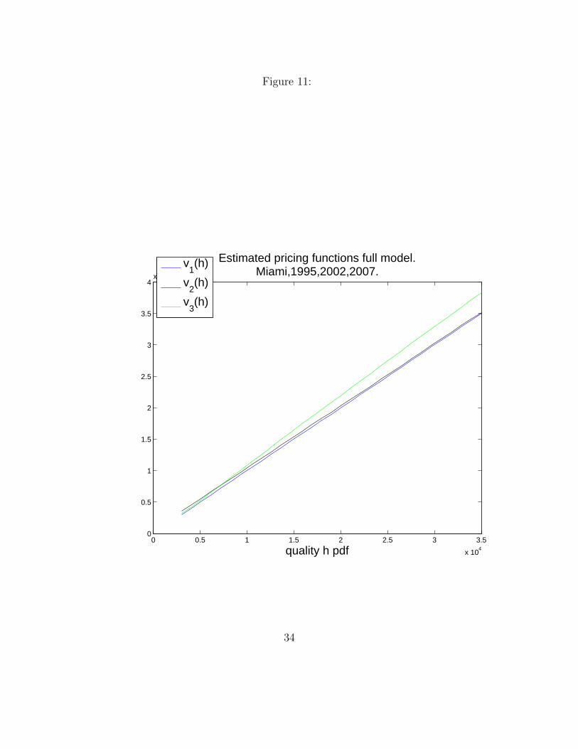
Figure 11:
0 0.5 1 1.5 2 2.5 3 3.5
x 104
0
0.5
1
1.5
2
2.5
3
3.5
4x 10
4
quality h pdf
Estimated pricing functions full model.Miami,1995,2002,2007.
v1(h)
v2(h)
v3(h)
34

rates for housing. Our finding s confirm this result.
6 Conclusions
We have developed a new approach for estimating the price-quality frontier in mar-
kets for durable housing. Our method has a number of advantages. First, it does
not require any a priori assumptions about the characteristics that determine house
quality. Second, it is easily implementable using metropolitan-level data on the distri-
bution of house values and the distribution of characteristics of households. Third, it
provides a straightforward summary of the changes in prices across the house quality
distribution. In particular, we do not need to collapse the change in the distribution
of prices into one number, as, for example, with the Case-Shiller index. Fourth, it
gives insights into the mechanism that generates those price changes. Finally, we
have shown that it provides some new insights into recent developments in local real
estate markets.
We apply our methods to study the housing markets of Miami. We find that our
model of nonlinear pricing in housing markets is consistent with the data observed
in Miami before and during the bubble period, if we allow for flexible specification
of the rent-to-value-functions that are consistent with the underlying structure of
our model. We find that the rent-to-value dropped by up to 50 percent from the
pre-bubble levels. Rents only increased moderately. These facts then account for the
large run-up in housing values and the much smaller change in rents that we observed
in Miami during the bubble period. Our findings are broadly consistent with the view
that changes in credit market conditions for low income houses together with changes
in investor expectations about future housing prices may have accounted for the large
run-up in housing values.
35

References
Bajari, P. and Benkard, L. (2005). Demand Estimation With Heterogeneous Con-
sumers and Unobserved Product Characteristics: A Hedonic Approach. Journal
of Political Economy, 113, 1239–77.
Bartik, T. (1987). The Estimation of Demand Parameters in Hedonic Price Models.
Journal of Political Economy, 95, 81–88.
Berry, S. and Pakes, A. (2007). The Pure Characteristics Demand Model. Interna-
tional Economic Review, 48 (4), 1193–1225.
Brueckner, J. and Rosenthal, S. (2005). Gentrification and Neighborhood Housing
Cycles: Will America’s Future Downtowns Be Rich?. Working Paper.
Dunz, K. (1989). Some Comments on Majority Rule equilibria in Local Public Goods
Economies. Journal of Economic Theory, 47, 228–234.
Ekeland, I., Heckman, J., and Nesheim, L. (2004). Identification and Estimation of
Hedonic Models. Journal of Political Economy, 112(1), S60–S101.
Epple, D. (1987). Hedonic Prices and Implicit Markets: Estimating Demand and
Supply Functions for Differentiated Products. Journal of Political Economy,
95, 59–80.
Glaeser, E. and Gyourko, J. (2005). Urban Decline and Durable Housing. Journal of
Political Economy, 113, 345–75.
Heckman, J., Matzkin, R., and Nesheim, L. (2010). Nonparametric Identification and
Estimation of Nonadditive Hedonic Models. Econometrica, 78(5), 1569–1591.
36

Henderson, J. V. and Venables, A. (2009). The Dynamics of City Formation. Review
of Economic Dynamics, 12 (233-54).
Landvoigt, D., Piazzesi, M., and Schneider, M. (2011). The Housing Market(s) of
San Diego. Working Paper.
Nechyba, T. (1997). Local Property and State Income Taxes: the Role of Interjuris-
dictional Competition and Collusion. Journal of Political Economy, 105 (2),
351–84.
Nechyba, T. (2000). Mobility, Targeting and Private School Vouchers. American
Economic Review, 90, 130–146.
Poterba, J. (1984). Tax Subsidies to Owner-Occupied Housing: An Asset-Market
Approach. Quarterly Journal of Economics, 99 (4), 729–52.
Poterba, J. (1992). Taxation and Housing: Old Questions, New Answers. American
Economic Review, 82 (2), 237–242.
Rosen, S. (1974). Hedonic Prices and Implicit Markets: Product Differentiation in
Pure Competition. Journal of Political Economy, 82, 34–55.
Sommer, K., Sullivan, P., and Verbrugge, R. (2011). Run-up in the House Price-Rent
Ratio: How Much Can Be Explained by Fundamentals?. BLS Working Paper.
Vianelli, S. (1983). The family of normal and lognormal distributions of order r.
Metron, 41, 3–10.
Wheaton, W. (1982). Urban Spatial Growth under Perfect Foresight. Journal of
Urban Economics, 12, 1–21.
37

A Proofs
Proof 1 The single-crossing condition implies that there is stratification of house-
holds by income in equilibrium. Stratification implies that there exists a distribution
function for house values Gt(v) such that:
Ft(y) = Gt(v) (31)
Hence there exists a monotonic mapping between income and housing value. If Ft is
strictly monotonic, it can be inverted, and hence F−1t exists. Q.E.D.
Proof 2 Equating the quantiles for income and value distributions, i.e. setting
Ft(yt(v)) = Gt(v) for yt > exp(µt)− βt, and vt > exp(ωt)− θt, yields:∫ [(ln(yt+βt)−µt)/σt]rt/rt0
e−tt1/rt−1dt
2rΓ(1 + 1/rt)=
∫ [(ln(vt+θt)−ωt)/τt]mt/mt0
e−tt1/mt−1dt
2mΓ(1 + 1/mt)(32)
Assuming rt = mt in each period, the quantiles are equal when
ln(yt + βt)− µtσt
=ln(vt + θt)− ωt
τt(33)
Similar steps lead to the same conclusion when yt < exp(µt)−βt, and vt < exp(ωt)−θt.
Solving (33) yields:
yt = e(µt−σtτt ωt)(vt + θt)
σtτt − βt (34)
Q.E.D.
Proof 3 The household’s FOC is:
αu′(h) · dh =dv
(yt − vt − κ)(35)
Substituting the income loci (8):
αu′(h)dh =dv
At(vt + θt)bt − βt − vt − κ
38

Since κ = θt − βt ∀t, the FOC becomes:
αiu′i(h)dh =
dv
At(vt + θt)bt − (vt + θt)(36)
Integrating the right hand side yields:∫dv
At(v + θt)bt − (v + θt)=
1
bt − 1
(ln
(− 1
At
(vt + θt − At (v + θt)
bt))− bt ln v + θt
)+ct
which implies:
αu(h) =1
bt − 1ln
(1− (vt + θt)
1−bt
At
)+ ct (37)
Notice that integrating the left hand side recovers the original function u(h). Using
the utility function we get
α ln(1− φ(h+ η)γ) =1
bt − 1ln
(1− (v + θt)
1−bi
At
)+ ct (38)
Solving for vt
(1− φ(h+ η)γ)α(bt−1) =
(1− (vt + θt)
1−bt
At
)ect (39)
and hence
vt =
(At
[1− (1− φ(h+ η)γ)α(bt−1)
ect
]) 11−bt
− θt (40)
Normalizing the constant of integration to c = 0 gives the result. Q.E.D.
Proof 4 We can write the household’s optimization problem as:
maxh
u1(h) + u2(y − v(h)) (41)
The FOC of this problem with respect to h is given by:
u′1(h)− u′2(y − v(h)) v′(h) = 0 (42)
39

Now define h∗ = v(h) and hence h = v−1(h∗). The decision problem associated with
this model is then
maxh∗
u1(v−1(h∗)) + u2(y − h∗) (43)
and the FOC with respect to h∗ is
u′1(v−1(h∗)) v−1′(h∗)− u′2(y − h∗) = 0 (44)
Now h = v−1(h∗) = v−1(v(h)) and hence v−1′(h∗) v′(h) = 1. Hence we conclude that
the two models are observationally equivalent. In the first case, we have non-linear
pricing and in the second case we have linear pricing. Q.E.D.
Proof 5 Recall from our discussion following Proposition 2 that parameters At, bt, θt
can be estimated directly from data for income and house rent distributions. We show
these are sufficient for identification of the utility function parameters. First consider
the normalization vt(h) = h. Recall that the equilibrium hedonic pricing function is
given by:
vt =(At
[1− [1− φ(h+ η)γ]α(bt−1)
]) 11−bt − θt (45)
Setting
α =1
bt − 1(46)
implies
vt = (At [1− [1− φ(h+ η)γ]])1
1−bt − θt = (Atφ(h+ η)γ)1
1−bt − θt (47)
Setting
φ =1
At(48)
implies
vt = ((h+ η)γ)1
1−bt − θt (49)
40

Setting
γ = 1− bt (50)
implies
vt = (h+ η)− θt (51)
Finally, setting
η = θt (52)
implies.
vt = h (53)
That establishes identification of the parameters of the utility function. The price
equation in period t+ s is then given by:
vt+s(h) =(At+s
[1− [1− φ(h+ η)γ]α(bt+s−1)
]) 11−bt+s − θt+s (54)
The parameters of joint value and income distribution in period t nail down the pa-
rameters of the utility function. The assumption of constant utility then imply that
vt+s(h) is fully identified by the parameters bt+s, At+s, and θt+s. Q.E.D.
Proof 6 Given our normalizations, we have also identified the housing supply func-
tion in the first period since R1(h) = G1(v) which then identifies the density of housing
quality in the first period q1(h).
Proposition 5 implies that v2(h) is identified. As a consequence G2(v2(h)) is identi-
fied. Moreover, V1(h) and V2(h) are observed by the econometrician. As a consequence
ζ is identified of the market clearing condition:
R2(h) = k2
∫ h
0
q1(x)
(V2(x)
V1(x)
)ζdx (55)
Q.E.D.
Note that this proof generalizes for more complicated parametric forms of the supply
function.
41

B The Generalized Lognormal Distribution with
Location (GLN4)
The generalized lognormal distribution with location GLN4 pdf is given by:
f(y) =1
2(x+ β)r1rσΓ
(1 + 1
r
)e− 1rσr| ln(x+β)−µ|r (56)
The CDF of the GNL4 distribution is given by:
Ft(y) =
Γ(
1r, B(y + β)
)2Γ(1
r)
for y < exp(µ)− β,
12
for y = exp(µ)− β,
12
+γ(
1r,M(y + β)
)2Γ(1
r)
for y > exp(µ)− β.
(57)
where
• B(y) =
[µ−log(y+β)
σ
]rr
, M(y) =
[log(y+β)−µ
σ
]rr
,
and
• Γ(s, z) =∈∞z e−ttv−1dt, γ(v, z) =∫ z
0e−ttv−1dt
are the incomplete gamma functions.
42