Embed Size (px)
Citation preview

WP/16/213
How to better measure hedonic residential property price indexes
by Mick Silver
IMF Working Papers describe research in progress by the author(s) and are published
to elicit comments and to encourage debate. The views expressed in IMF Working Papers
are those of the author(s) and do not necessarily represent the views of the IMF, its
Executive Board, or IMF management.
2
© 2016 International Monetary Fund WP/16/213
IMF Working Paper
Statistics Department
How to better measure hedonic residential property price indexes
Prepared by Mick Silver1
Authorized for distribution by Claudia Dziobek
November 2016
Abstract
Hedonic regressions are used for property price index measurement to control for changes in
the quality-mix of properties transacted. The paper consolidates the hedonic time dummy
approach, characteristics approach, and imputation approaches. A practical hedonic
methodology is proposed that (i) is weighted at a basic level; (ii) has a new (quasi-)
superlative form and thus mitigates substitution bias; (iii) is suitable for sparse data in thin
markets; and (iv) only requires the periodic estimation of hedonic regressions for reference
periods and is not subject to the vagrancies of misspecification and estimation issues.
JEL Classification Numbers: C43, E30, E31, R31.
Keywords: Hedonic Regressions; Residential Property Price Index; Commercial Property
Price Index; House Price Index; Superlative Index Number; Thin Property Markets.
Author’s E-Mail Address: [email protected]
1 The author acknowledges comments by Gabriela Maciel (IMF, Research Department) and participants at the
2016 Conference of the Society of Economic Measurement, Thessaloniki, Greece, July 2016.
IMF Working Papers describe research in progress by the author(s) and are
published to elicit comments and to encourage debate. The views expressed in
IMF Working Papers are those of the author(s) and do not necessarily represent the
views of the IMF, its Executive Board, or IMF management.
3
Contents Page
Abstract ......................................................................................................................................2
I. Introduction ............................................................................................................................4 A. The problems.............................................................................................................4
B. The paper .................................................................................................................10
II. Measures of hedonic constant-quality property price change .............................................12 A. Hedonic regressions ................................................................................................12 B. The time dummy variable approach. .......................................................................16 C. The characteristics approach ...................................................................................23
D. The imputation approach ........................................................................................30 E. An indirect approach to hedonic price indexes .......................................................32
F. Arithmetic versus geometric aggregation: how much does it matter? ....................35
III. Some equivalences .............................................................................................................39
IV. Weights and superlative hedonic price indexes .................................................................43 A. Lower-level weights for a linear/arithmetic hedonic formulation ..........................45
B. Log-linear hedonic model .......................................................................................49 C. The nature of substitution bias for a hedonic price index .......................................51
D. Hedonic superlative indexes and sample selection bias..........................................52
E. Hedonic superlative price index number formulas: Hill and Melser (2008) ...........54
F. Weights for the time dummy approach ...................................................................57 G. Stock weights ..........................................................................................................60
V. Hedonic property price indexes series: periodic rebasing, chaining and rolling windows .61
VI. A practical choice of formula: equivalences, infrequent hedonic estimation, weighting,
thin markets, and the indirect approach ...................................................................................64
VII. Summary ..........................................................................................................................75
Tables
1. Illustrative linking of results from rolling window regression ............................................22 2. Illustration of periodic linking .............................................................................................61 3. Rolling window regression example ....................................................................................62
4. Illustration of quarterly adjacent period chaining ................................................................64
Annexes
A. Difference between hedonic arithmetic and geometric mean property price .....................76 B. Outliers and leverage effects on coefficient estimates. .......................................................79
C. Equating an estimated coefficient on a time dummy from a log-linear hedonic model to
the geometric mean of the price changes .................................................................................80
References ................................................................................................................................82
4
I. INTRODUCTION
A. The problems
Macroeconomists and central banks need measures of residential property price inflation.
They need to identify bubbles, the factors that drive them, instruments that contain them, and
analyze their relation to recessions.2 Such measures are also needed for the System of
National Accounts and may be needed as part of the measurement of owner-occupied
housing in a consumer price index—see Eurostat et al. (2013, chapter 3). Timely,
comparable, proper measurement is a prerequisite for all of this, driven by concomitant data.
There have been major advances in this area foremost of which are: (i) recently developed
international standards on methodology, the Eurostat et al. (2103) Handbook on Residential
Property Price Indices (RPPIs);3 (ii) an impressive array of data hubs dedicated to the
dissemination of house price indices and related series including the IMF’s Global Housing
Watch; the Bank for International Settlements’ (BIS) Residential Property Price Statistics;
the OECD Data Portal; the Federal Reserve Bank of Dallas’ International House Price
Database; Eurostat Experimental House Price Indices; and private sources;4 and (iii)
encouragement in compiling and disseminating such measures: real estate price indexes are
included as Recommendation 19 of the G-20 Data Gaps Initiative (DGI), and residential
property price indexes are prescribed within the list of IMF Financial Soundness Indicators
(FSIs), in turn included in the IMF’s new tier of data standards, the Special Data
Dissemination Standard (SDDS) Plus.5 In this paper we identify the challenges countries face
in the hard problem of measuring hedonic residential property price indexes (RPPIs). While
2 For salient papers see the recent Conference by Deutsche Bundesbank, the German Research Foundation
(DFG) and the International Monetary Fund on “Housing Markets and the Macroeconomy: Challenges for
Monetary Policy and Financial Stability” at:
http://www.bundesbank.de/Redaktion/EN/Termine/Research_centre/2014/2014_06_05_eltville.html
3 http://epp.eurostat.ec.europa.eu/portal/page/portal/hicp/methodology/hps/rppi_handbook.
4 The IMF’s Global Housing Watch provides current data on house prices for 52 countries as well as metrics
used to assess valuation in housing markets, such as house price-to-rent and house-price-to-income ratios:
http://www.imf.org/external/research/housing/; the BIS has extensive country series on RPPIs along with details
of, and links to, country metadata and source data: http://www.bis.org/statistics/pp.htm; OECD also
disseminates country house price statistics and is developing a wide range of complementary housing statistics:
http://www.oecd.org/statistics/; see also the Federal Reserve Bank of Dallas’ International House Price
Database, Mack and Martínez-García (2011), at: http://www.dallasfed.org/institute/houseprice/index.cfm and
Eurostat Experimental House Price Indices at:
http://appsso.eurostat.ec.europa.eu/nui/show.do?dataset=prc_hpi_q&lang=en.
5 The setting of such standards is a key element of Recommendation 19 of the report: The Financial Crisis and
Information Gaps, endorsed at the meeting of the G-20 Finance Ministers and Central Bank Governors on
November 7, 2009 and carries over for RPPIs and CPPIs to individual recommendations under the follow-up
DGI-2; see Heath (2013) for details of SDDS Plus and the DGI and http://fsi.imf.org/ for FSIs under “concepts
and definitions.”
(continued…)
5
the focus of the paper will be on RPPIs, the analysis and proposed methodology holds for the
more difficult area of hedonic commercial property prices indexes (CPPIs). Indeed, the
problem of infrequent transactions and property heterogeneity are more profound for CPPIs
than RPPIs and the proposals in this paper for dealing with sparse data in thin markets more
relevant.
We first, in this sub-section IA of the “Introduction” to the paper, provide a context to the
paper by outlining the problem of RPPI measurement.6 In the next sub-section, IB, we
outline the purpose and structure of the paper.
The problem of quality-mix adjustment
Critical to price index measurement is the need to compare, in successive periods, transaction
prices of like-with-like representative goods and services. Price index measurement for
consumer, producer, and export and import price indexes (CPI, PPI and XMPIs) largely rely
on the matched-models method. The detailed specification of one or more representative
brand is selected as a high-volume seller in an outlet, for example a single 330 ml. can of
regular Coca Cola, and its price recorded. The outlet is then revisited in subsequent months
and the price of the self-same item recorded and a geometric average of its price and those of
similar such specifications in other outlets form the building blocks of a price index such as
the CPI. There may be problems of temporarily missing prices, quality change, say size of
can or sold as a bundled part of an offer if bought in bulk, but essentially the price of like is
compared with like every month.7 RPPIs are much harder to measure.
First, there are no transaction prices every month/quarter on the same property. RPPIs have
to be compiled from infrequent transactions on heterogeneous properties. A higher
(lower) proportion of more expensive houses sold in one quarter should not manifest itself as
a measured price increase (decrease). There is a need in measurement to control for
changes in the quality of houses sold, a non-trivial task.
The main methods of quality adjustment are (i) hedonic regressions; (ii) use of repeat sales
data only; (iii) mix-adjustment by weighting detailed relatively homogeneous strata; and (iv)
the sales price appraisal ratio (SPAR).8 The method selected depends on the database used.
There needs to be details of salient price-determining characteristics for hedonic regressions,
6 We draw on Silver (2016a) for this sub-section IA.
7 International manuals on all of these indexes can be found at under “Manuals and Guides/Real Sector” at:
http://www.imf.org/external/data.htm#guide. This site includes the CPI Manual: International Labour Office et
al. (2004).
8 Details of all these methods are given in Eurostat et al. (2013); see also Hill (2013) for a survey of hedonic
methods for residential property price indexes; Silver and Heravi (2007) and Diewert, Heravi, and Silver (2008)
on hedonic methods; Diewert and Shimizu (2013b) and Shimizu et al. (2010) for an application to Tokyo; and
Shiller (1991, 1993, and 2014) on repeat-sales methodology.
6
a relatively large sample of transactions for repeat sales, and good quality appraisal
information for SPAR. In the US, for example, price comparisons of repeat sales are mainly
used, akin to the like-with-like comparisons of the matched models method, Shiller (1991).
There may be bias from not taking full account of depreciation and refurbishment between
sales and selectivity bias in only using repeat sales and excluding new home purchases and
homes purchased only once. However, the use of repeat sales does not require data on quality
characteristics and controls for some immeasurable characteristics that are difficult to
effectively include in hedonic regressions, such as a desirable or otherwise view from the
property.
The problem of source data
Second, the data sources are generally secondary sources that are not tailor-made by the
national statistical offices (NSIs), but collected by third parties, including the land
registry/notaries, lenders, realtors (estate agents), and builders. The adequacy of these
sources to a large extent depends on a country’s institutional and financial arrangements for
purchasing a house and varies between countries in terms of timeliness, coverage (type,
vintage, and geographical), price (asking, completion, transaction), method of quality-mix
adjustment (repeat sales, hedonic regression, SPAR, square meter) and reliability; pros and
cons will vary within and between countries. In the short-medium run users may be
dependent on series that have grown up to publicize institutions, such as lenders and realtors,
as well as to inform users. Metadata from private organizations may be far from satisfactory.
We stress that our concern here is with measuring RPPIs for FSIs and macroeconomic
analysis where the transaction price, that includes structures and land, is of interest.
However, for the purpose of national accounts and analysis based thereon, such as
productivity, there is a need to both separate the price changes of land from structures and
undertake adjustments to price changes due to any quality change on the structures, including
depreciation. This is far more complex since separate data on land and structures is not
available when a transaction of a property takes place. Diewert, de Haan, and Hendriks
(2011) and Diewert and Shimizu (2013a) tackle this difficult problem.
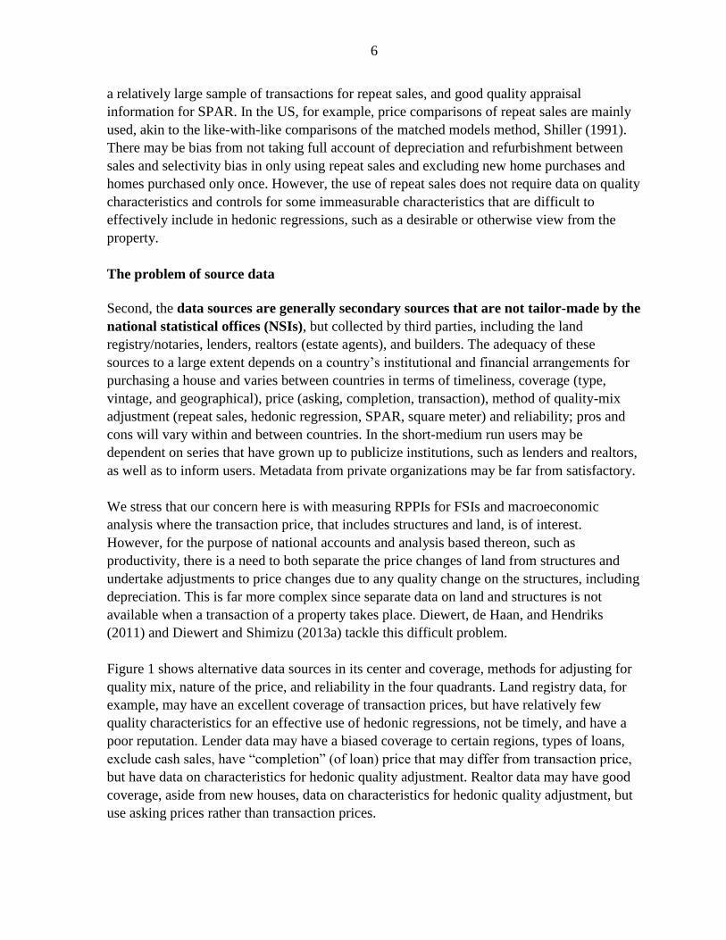
Figure 1 shows alternative data sources in its center and coverage, methods for adjusting for
quality mix, nature of the price, and reliability in the four quadrants. Land registry data, for
example, may have an excellent coverage of transaction prices, but have relatively few
quality characteristics for an effective use of hedonic regressions, not be timely, and have a
poor reputation. Lender data may have a biased coverage to certain regions, types of loans,
exclude cash sales, have “completion” (of loan) price that may differ from transaction price,
but have data on characteristics for hedonic quality adjustment. Realtor data may have good
coverage, aside from new houses, data on characteristics for hedonic quality adjustment, but
use asking prices rather than transaction prices.
7
The importance of distinguishing between asking and transaction prices will vary between
countries as the length of time between asking and transaction varies with the institutional
arrangements for buying and selling a house and the economic cycle of a country.
Whether measurement matters
A natural question is whether the differences in source data and methodologies used matters
to the overall outcome of the index. Silver (2015) undertook an extensive formal analysis
based on the RPPIs and, as explanatory variables, the associated methodological and source
data for 157 RPPIs from 2005:Q1 to 2010:Q1 from 24 countries. The resulting panel data had
fixed-time and fixed-country effects; the estimated coefficients on the explanatory
measurement variables were first held fixed and then relaxed to be time varying.
Subsequently, the explanatory variables were interacted with the country dummies.
t Figure 1. Methodological issues and data sources in RPPI measurement
He found measurement-related variables as explanatory variables for house price inflation
had substantial explanatory power,2R , especially over the period of recession, when it really
matters, about 0.45 in mid-2009. He further investigated the impact of measurement on
modelling, using an econometric model of house price inflation based on Igan and Loungani
8
(2012). Using the residuals from the regression of house price index on measurement
variables
as a “measurement-adjusted” house price index he found the measurement-adjusted model to
perform better than the unadjusted one. Less formally, he provided some country
illustrations. 9
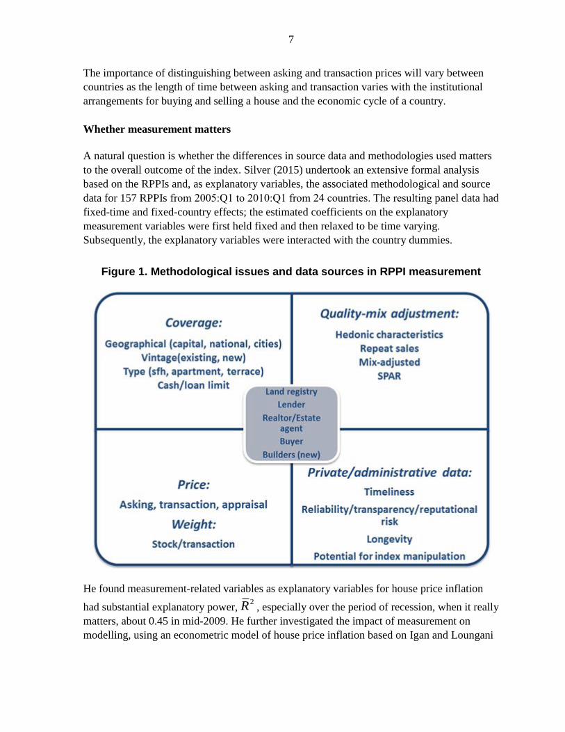
Figure 2 shows a feast of RPPIs
available for the UK including the
ONS (UK, hedonic mix-adjusted,
completion price); Nationwide and
Halifax (both UK, hedonic, own
mortgage approvals, mortgage offer
price; Halifax weights); the England
and Wales (E&W) Land Registry
(E&W, repeat sales, all transaction
prices); and the ONS Median price
index unadjusted for quality mix—
given for comparison.10 Other available
RPPIs in the UK are LSL Acadata HPI
(Land registry), 11 Right move (realtor)
and two RPPIs based on surveys of
expert opinion. Measured inflation in
2008Q4 coming into the trough was -
8.7 (ONS) -12.3 (Land registry) -16.2
(Halifax) -14.8 (Nationwide): and -4.9
(ONS Median unadjusted (for quality
mix change); methodology and data
source matter.
9 Data are generally sourced from: http://www.bis.org/statistics/pp.htm use also being made of:
http://www.acadata.co.uk/acadHousePrices.php; http://www.ons.gov.uk/ons/rel/hpi/house-price-index/july-
2014/stb-july-2014.html; http://us.spindices.com/index-family/real-estate/sp-case-shiller; and
http://www.fhfa.gov/KeyTopics/Pages/House-Price-Index.aspx
10 A detailed account of the methodologies and source data underlying these RPPIs for the UK is given in
Matheson (2010), Carless (2013), and ONS (2013); see also http://www.ons.gov.uk/ons/guide-method/user-
guidance/prices/hpi/index.html.
11 Acadata use a purpose built “index of indices” forecasting methodology to help “resolve” the problem that
only 38 percent of sales are promptly reported to Land Registry, considered by Acadata to be an insufficient
sample to be definitive. The LSL Acad HPI “forecast” is updated monthly until every transaction is included.
Effectively, an October LSL Acad E&W HPI “final” result, published with the December LSL Acad HPI
“forecast” is definitive.
Figure 2. A Feast of UK RPPIs, annual percent rate, quarterly
9
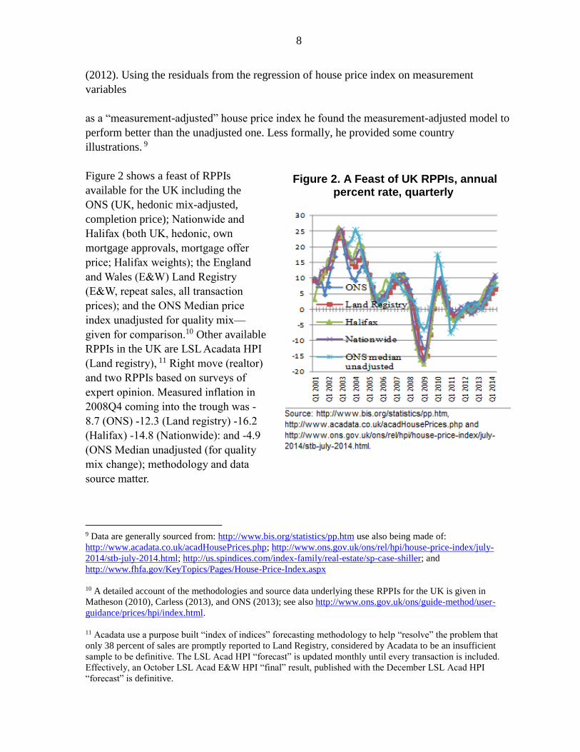
Figure 3 shows RPPIs available in the
US including the: CoreLogic, Federal
Housing Finance Agency (FHFA)
purchases-only, Case-Shiller, and the
FHFA extended-data House Price Index
(HPI). CoreLogic, FHFA, and Case-
Shiller, the three primary RPPIs in the
US, use repeat sales for quality-mix
adjustment—the Census Bureau is a
(hedonic) new houses only index based
on a limited sample. The FHFA
extended-data HPI includes, in addition
to transaction prices from purchase-
money mortgages guaranteed by Fannie
Mae and Freddie Mac, transactions
records for houses with mortgages
endorsed by the Federal Housing
Administration (FHA) and county
recorder data licensed from CoreLogic,
appropriately re-weighted to ensure
there is no undue urban over rural bias. This change in source data coverage accounted for
the 4.6 percentage point difference in 2008 Q4 between the annual quarterly RPPI respective
falls of 6.89 and 11.66 percent for the FHFA “All Purchases” and “Extended-Data” FHFA
HPIs. Coverage limited to particular types of mortgages matters.12
Leventis (2008) decomposed into methodological and coverage differences the average
difference between the FHFA (then Office of Federal Housing Enterprise Oversight
(OFHEO)) and S&P/Case-Shiller HPIs, covering 10 matched metropolitan areas, for the
four-quarter price changes over 2006Q3-2007Q3. Among his findings was that of the overall
4.27 percent average difference, FHFA’s use of a more muted down-weighting of larger
differences in the lags between repeat sales,13 than use in Case-Shiller, accounts for an
12 http://www.fhfa.gov/PolicyProgramsResearch/Research/Pages/Recent-Trends-in-Home-Prices-Differences-
across-Mortgage-and-Borrower-Characteristics-.aspx.
13 The S&P/Case-Shiller methodology materials suggest that its down-weighting is far more modest than
FHFA. Over longer time periods, evidence suggests that there is greater dispersion in appreciation rates across
homes. This variability causes heteroskedasticity, which increases estimation imprecision. The down-weighting
mitigates the effect of the heteroskedasticity. Leventis (2008, page 3) notes that the S&P/Case-Shiller
methodological material suggest valuation pairs, which reflect the extent to which homes have appreciated or
depreciated over a known time period, are given 20-45 percent less weight when the valuations occur ten years
apart vis-à-vis when they are only six months apart. By contrast, OFHEO’s down-weighting tends to give ten-
year pairs about 75 percent less weight than valuation pairs with a two-quarter interval. Differences in filters
and coverage of qualifying loans (FHFA) account for much of the rest.
Figure 3. US Repeat sales RPPIs, annual percent change, quarterly
10
incremental 1.17 percent of the difference. It is not just that the use of different quality-mix
adjustment methods matters, it does also the manner in which a method is applied.
B. The paper
This paper examines, consolidates, and provides improved practical methods for the timely
estimation of hedonic RPPIs, though, as noted earlier, the proposed methods apply equally to
CPPIs. Hedonic regressions are the main mechanism recommended for and used by countries
for a crucial aspect of RPPI estimation—preventing changes in the quality-mix of properties
transacted translating to price changes.
RPPIs and CPPIs are hard to measure. Houses, never mind commercial properties, are
infrequently traded and heterogeneous. Average house prices may increase over time, but this
may in part be due to a change in the quality-mix of the houses transacted; for example, more
4-bedroom houses in a better (more expensive) post-code transacted in the current period
compared with the previous or some distant reference period would bias upwards a measure
of change in average prices. A purpose and crucial challenge of RPPIs and CPPIs is to
prevent changes in the quality-mix of properties transacted translating to measured price
changes. The need is to measure constant-quality property price changes and while there are
alternative approaches,14 the concern of this paper is with the hedonic approach as a
recommended widely used methodology for this. 15
The aim of this paper is to further develop a best practice methodology grounded in both the
practical considerations and methodological rigor required for such an important statistic.
The methodology is consistent with, but extends the provisions in, the 2013 Handbook on
RPPIs (Eurostat et al., 2013) that form the international standards in this area.
The hedonic approach identifies properties as tied bundles of characteristics. The
characteristics
14 Alternatives include repeat sales, mix-adjustment by weighting more-homogeneous strata, and the sales price
appraisal ratio (SPAR) are further alternatives. Each is used to form constant quality price indexes, SPAR by
using the relationship between appraisal and transaction prices where such data coexist and predicting
transaction prices. Repeat sales only uses that part of the dataset where there is more than one transaction over a
given period. Details of all these methods are given in Eurostat et al. (2013); see also Hill (2013) for a survey of
hedonic methods for residential property price indexes; Silver and Heravi (2007a) and Diewert, Heravi, and
Silver (2009) on hedonic methods; Diewert and Shimizu (2013b) and Shimizu et al. (2010) for applications to
Tokyo; and Shiller (1991, 1993, and 2014) on repeat-sales methodology., though see Case, Pollakowski, and
Watcher (2003) for a hybrid repeat sales and hedonic model applied to house price indexes.
15 Hill (2013, 906) concludes his survey paper: “Hedonic indexes seem to be gradually replacing repeat sales as
the method of choice for constructing quality-adjusted house price indexes. This trend can be attributed to the
inherent weaknesses of the repeat sales method (especially its deletion of single-sales data and potential lemons
bias) and a combination of the increasing availability of detailed data sets of house prices and characteristics,
including geospatial data, increases in computing power, and the development of more sophisticated hedonic
models that in particular take account of spatial dependence in the data.”
11
are the price-determining ones, including size of property, number of bedrooms, location and
so forth, and the sense in which they are “tied” is that the characteristics are not sold
separately—there is no price in the market for each characteristic, only one for the house,
structure and land, as a whole. Were there a price for a say additional bathroom, and houses
transacted in the current period had more bathrooms, on average, we would have the means
by which constant quality property price changes could be estimated. A hedonic regression of
property prices on property characteristics allows us to “unbundle” the overall price and give
estimated marginal values to the individual characteristics. This paper tackles the important
question as to how, given estimated hedonic regressions, do we best compile hedonic,
constant-quality, property price indexes?
The Handbook on Residential Property Price Indices (RPPIs) (Eurostat et al., 2013) provides
international guidelines on RPPI measurement and chapter 5 contains three hedonic
approaches—the hedonic time dummy approach, characteristics approach, and imputation
approach. This follows previous literature in this area including Triplett (2006), Silver and
Heravi (2007a) and Hill (2013). A problem is that there are many alternative forms for each
approach depending on which period estimated hedonic coefficients, characteristic baskets,
and weights are held constant, whether dual or single imputation is used for either prices or
weights, a direct or indirect formulation is used, chained, rolling window or fixed baskets of
characteristics, and more.
We first outline in section II the alternative approaches to hedonic property price indexes to
ground the analysis. Throughout the paper this is undertaken for both linear and log-linear
hedonic specification. In section III we demonstrate, for reasonable specifications of hedonic
regressions, equivalences between the approaches and consolidate them to show that hedonic
imputation and characteristics approaches yield the same result and the time dummy can be
formulated as being a close approximation. The resulting formulas benefit from being
justified by the different intuitions of the approaches.
In section IV we devise a weighting system for property price change at the elementary level,
in this case for the price change of each individual property—an issue highlighted by Diewert
(2005a). This is undertaken for the hedonic imputation approach but, due to the equivalences
of the approaches, can also be mirrored in the characteristics approach to give the same
result. While arithmetic (linear) formulation has a fortuitous implicit weighting system;
however, the log-linear (geometric) price index equally weights property price changes. We
develop for the log-linear (geometric) case a means by which explicit weights can be readily
applied. Having done so, a natural next step is to define a superlative hedonic price index that
makes symmetric use of reference period and current period weights. This is undertaken in
two steps by defining hedonic “quasi-superlative” and re-defining “hedonic superlative”
property price indexes, to advance on existing formulations in the literature of these target
measures. The analysis so far is for bilateral price index number measurement, that is
12
between a reference period and a current period. Section V extends the analysis to cover
linking and chaining these bilateral indexes over time.
Practical problems are considered arising out of a concern with thin markets—sparse
transaction price data. Controlling for the effect of heterogeneous properties requires a
concomitant generous hedonic specification and care with estimation that is ill-served by
frequent
re-estimation using sparse data. It is particularly important to ground the hedonic price
comparisons in a reference period that is relatively exhaustive of the property mix that arises
in subsequent periods. The concern of the proposed methods is for parsimony of estimation,
that is to not rely on estimates in successive periods and that better formulated to deal with
sparse data.
In section VI a useful practical measure for countries is developed. The measure (i) benefits
from a focus on the imputation approach, which is conducive to weighting, which provides
equivalent result to the characteristics approach; (ii) requires that a hedonic regression only
be run for the reference period;16 (iii) better accommodates sparse transaction data in thin
markets; (iv) incorporates a quasi-superlative weighting system at the elementary level; (v)
adopts an indirect approach to facilitate the use of dual imputations but also aids in
interpretation; and (vi) can be readily extended as a conventional hedonic superlative index
for retrospective studies.
II. MEASURES OF HEDONIC CONSTANT-QUALITY PROPERTY PRICE CHANGE
A. Hedonic regressions
The price index number problem for real estate is that measures of changes in the average
price of properties reflect in part changes in the quality-mix of properties transacted. For
example, there may be more 2-bedroom apartments sold in the current period than in some
reference period. One way of tackling this problem is to determine the (marginal) value of an
additional unit of each price-determining quality characteristic, such as the number of
bedrooms, bathrooms, square footage of property, floor of apartment, possession or
otherwise of parking, balcony, postcode, proximity to a metro, quality indicator of local
school, and so forth. But such characteristics are not priced on the market, only the property
as a whole.
Estimated hedonic regression equations explain variation in property prices, on the left hand
side (LHS) of the equation, in terms of explanatory price-determining characteristics on the
16 Though some re-estimation, say every year or two years, much like rebasing a consumer price index, would
be advised, as would separate estimates for meaningful strata, say defined by location and type, for example,
single family homes in the capital city.
(continued…)
13
right hand side (RHS). The coefficients on each RHS characteristic are estimates of the
marginal value of each respective characteristic.17 By considering properties as tied bundles
of characteristics with associated estimated marginal values, we are equipped to solve the
problem of adjusting changes in average property prices for changes in the quality-mix of
properties transacted.
Our starting point is an estimated hedonic regression for a stratum of properties in a country,
say apartments in the inner area of a capital city. The principles governing the specification
and estimation of hedonic regressions are not the subject of this paper.18 Our concern is how
hedonic regressions are used to derive property price indexes. Yet there is one issue that has
a direct bearing on the derivation of hedonic price indexes and that is the functional form of
the hedonic regression. Outlined here are two functional forms that are widely used, the latter
more so: a linear and log-linear form. Choice between these forms should be based on a
priori and empirical grounds (testing), as outlined in Halvorsen and Pallakowski (1981),
Cassel and Mendelsohn (1985), Can (1992), and Triplett (2006).
Functional forms of the hedonic regression: a linear form
Consider a linear hedonic functional form. An estimated hedonic regression would have the
prices, t
ip of an individual property i on the LHS and their associated k characteristics, ,
t
k iz on
the RHS as explanatory variables. Such hedonic regressions may be estimated for each
defined stratum in a period 0 reference period (index =100.00) and each successive period t
(=1,2,..,T). The linear functional form for period t is given by:
(1)…. 0 ,
1
( )K
t t t t t t t t
i k k i i i i
k
p z h z
and estimated as:
(2)…. 0 ,
1
ˆ ˆˆ ( )K
t t t t t t
i k k i i
k
p z h z
where ˆ t
ip (and t
ip ) are the predicted (actual) price of property i in period t; ,
t
k iz are the values
of each k=1,….,K price-determining characteristic for property i in period t; 0 and k (and,
below, 0 and k below) are the coefficients from a linear (and log-linear) hedonic equation;
17 See Rosen (1975), Feenstra (1995), Diewert (2003b), Pakes (2003), and Silver (2004) for the theoretical basis
of price indexes based on hedonic regressions.
18 Readers are referred to Berndt (1991) and Triplett (2006) for a clear overview of hedonic regression methods,
albeit not in the context of house prices, and for real estate: Sirmans et al (2006) on explanatory variables for
the hedonic regression, de Haan and Diewert (2013), Coulson (2008), and Pace and LeSage (2004), Hill and
Scholz (2013) and Silver and Graf (2012) for the increasing work on the spatial econometric modeling of house
prices.
14
t
i (and t
i ) i.i.d errors; and ( )t t
ih z a shorthand for a linear hedonic function estimated using
period t data and period t characteristics.
Equation (1) has prices explained by a constant, 0
t , slope coefficients t
k for each k price-
determining characteristics, ,
t
k iz , of which there are K , and an error term, t
i . It is a linear
relationship dictated, in equation (2), by the estimated constant and the slope coefficients,
represented as hats “^” over the coefficients; for a single characteristic: 0 1 1,ˆ ˆˆ t t t t
i ip z .
The actual relationship may be non-linear and there will be omitted variable bias in using a
linear form to (mis)represent the relationship. To counter this bias one possibility is to
introduce some curvature via a squared term, 2
0 1 1, 2 1,ˆ ˆ ˆˆ t t t t t t
i i ip z z , and test a null
hypothesis as to whether 2 0t , that is, whether the squared term has any explanatory power
over and above that due to sampling error, say at a five percent level of significance.
Interaction terms between more than one explanatory variable may also be introduced,
Maddala and Lahiri (2009).
Functional forms of the hedonic regression: a log(arithmic)-linear form
An alternative functional form is a log(arithmic)-linear—also referred to as a
semi-logarithmic—form of the hedonic regression. This form arises from a hedonic
relationship between t
ip and ,
t
k iz given by:
(3)…. ,1 ,2 ,
0 1 2 ,......,t t ti i i Kz z z
t t t t t t
i K ip
The log-linear form first allows for curvature in the relationships say between square footage
and price, and second, for a multiplicative association between quality characteristics, i.e.
that possession of a garage and additional bathroom may be worth more than the sum of the
two. The estimation of ordinary least squares regression (OLS) equations requires a linear
form; we transform the non-linear functional relationship in equation (3) into a linear form by
taking logarithms of both sides of the equation and use OLS:
(4)…. 0 ,
1
ln ln ln lnK
t t t t t
i k i k i
k
p z
= ( )t t t
i ih z
where the tilde across ( )t t
ih z designates a log-linear functional form. An OLS regression
estimated for the logarithm of prices, ˆln t
ip , on characteristics, ,
t
k iz , is given as:
15
(5)…. 0 , ,
1 0
ˆ ˆ ˆˆln ln ln ln ( )K K
t t t t t t t t
i k i k k i k i
k k
p z z h z
It is important to note that the log-linear regression output from estimating equation (4), that
is ln t
ip on ,
t
k iz , provides us with the logarithms of the coefficients from the original log-
linear formulation in equation (3). Exponents of the estimated coefficients from the output of
the software have to be taken if the parameters of the original function, that is equation (3),
are to be recovered, that is: ˆ ˆexp ln t t
k k .19
Since many explanatory variables are dummy variables taking a value of zero or
one—possession or otherwise of a characteristic—and since logarithms cannot be taken of
zero values, the log-linear form is more convenient than a double-logarithmic transformation
that would require logarithms be taken of the ,
t
k iz on the RHS. It should be noted that the
interpretation of coefficients from a log-linear form differs from that of coefficients from a
linear form. For a log-linear form our estimated coefficients are the logarithms of
1 2 3ˆ ˆ ˆ, ,and : a unit change in the say square footage,
1,iz , leads to a 1 percent change in
price, while for a dummy explanatory variable, say “possession of a balcony,2, 1iz as
opposed to 2, 0iz otherwise,” leads to an estimated 2exp 1 100 percent change in
price, as will be explained in more detail in the next section.
We consider in this paper that hedonic regressions take a generally applicable linear and
lo-linear forms given by equations (2) and (5) and that these have been estimated. Outlines of
the three main hedonic approaches to deriving constant quality price indexes from these
estimated equations, along their relative merits, are given below in sections B, C and E.
These approaches are the (i) hedonic time dummy variable, (ii) hedonic characteristics and
(iii) hedonic imputation approaches. The approaches are outlined and discussed in the
context of bilateral period 0 (reference period =100.00) and current period t price level
comparisons where t=1,2,….,T. While our main concern will be with quarter-on-quarter
inflation rates, the principles can be readily extended to quarter-on-same quarter in previous
year, though see Rambaldi and Rao (2103). The concern of section F is with the periodic
updating or chaining of the reference period estimates.
19 Again squared terms and cross-product interaction terms can be added to increase the flexibility of the
functional form to better represent underlying relationships.
16
B. The time dummy variable approach.
The method
A single hedonic regression equation may be estimated from data across properties over
several time periods including the reference period 0 and successive subsequent periods t.
Prices of individual properties are regressed on their characteristics, but also on dummy
variables for time, taking the values of 1 if the house is sold in period 1, and zero otherwise,
2 if the house is sold in period 2 and zero otherwise,…., T if the house is sold in period T
and zero otherwise. We exclude in this case a period 0 dummy time variable and interpret the t as the difference between the current period and reference period 0 average prices, having
controlled for quality-mix change via the variables in the hedonic regression on their
characteristics. The method has been widely applied including Fisher, Geltner, and Webb
(1994), Hansen, (2009), and Shimizu et al. (2010).
Consider a linear form of the hedonic regression given by equation (1) but estimated over
say two adjacent periods, 0 and 1:
(6)….0,1 1 1 0,1 0,1
0 ,
1
K
i i k k i i
k
p D z
The data for prices and characteristics extend over the two periods 0 and 1, yet only a single
parameter, k , is estimated for each characteristic’s slope coefficient. The restriction is that
the slopes of the regression lines for period 0 and period t are the same: 0 t
k k k for each
of k=1,….,K characteristics.
For simplicity, consider a single explanatory variable, the square footage of an individual
apartment, 0 1ori iz z in periods 0 and 1 respectively. Separate regression equations can be
estimated for each of period 0 and period 1, but the slope coefficient, the estimated marginal
value of an additional square foot, is restricted to be the same in each period, namely 1 :
(7a)…. 0 0 0 0
0 1i i ip z for period 0, and
(7b)…. 1 1 1 1
0 1i i ip z for period 1.
The estimated coefficients on the intercepts in each period are respectively 0
0 and 1
0 . These
are estimates of the average price in periods 0 and 1 having controlled for variation in the
square footage of the apartments—the “average” is an arithmetic mean for this linear
formulation (and a geometric mean for a log-linear formulation).
17
We can represent equations (7a and b) in a single hedonic regression:
(8)…. 0,1 0 1 1 0,1 0,1 0 1 0 1 0,1 0,1
0 1 0 0 0 1i i i i i i ip D z D z
The dummy variable 1
iD in equation (8) is equal to 1 if the data are in period 1, and zero
otherwise and its estimated coefficient 1 1 0
0 0ˆ ˆ ˆ . This representation of equations 7a
and 7b can be seen by inserting 1 0iD (period 0 data) into the RHS term of equation (8) to
give equation (7a) and inserting 1 1iD (period 0 data) to give equation (7b), assuming
0,1 0 1
i i iE E E .
The estimated coefficient on the dummy variable, 1 , is the basis for an estimate of a
constant quality property price index between periods 0 and 1. The estimate is of the
difference between the period 0 and period 1 intercepts,20 that is the difference in the average
prices of period 1 and period 0 transactions from their regression lines for period 0 and
period 1 having controlled for variation in the quality characteristics 0,
,
1
Kt
k k i
k
z
, as in equation
(6), whereby each k characteristic is valued at its associated ˆk .
A log-linear specification is given by:
(9).…0, 0,
0 ,
1 1
ln lnK T
t t t t t
i k i k i i
k t
p z D
The ˆt are estimates of the proportionate change in price arising from a change between the
reference period t=0—the period not specified as a dummy time variable—and successive
periods t=1,…,T having controlled for changes in the quality characteristics via the term
0,
,
1
Kt
k k i
k
z
.
The constant-quality price index is given for each period t=1,..,T, with respect to period t=0,
which equals 100.00, by ˆ100 exp( )t . In principle ˆ100 exp( )t requires an adjustment—
20 It may be thought that this interpretation is for the intercepts only when the explanatory variables are zero, but
this is not the case. By restricting the slope coefficients to be the same, the regression lines for equations 7(a)
and 7(b) run in parallel and the difference in the intercepts is the same for any value of the 0,1
,k iz characteristics.
(continued…)
18
for it to be a consistent (and almost unbiased) approximation of the proportionate impact of
the time dummy. The adjustment is given by: exp exp( / 2)) 1ˆ ˆV
t t,where ( )ˆV t
is the
variance (standard error squared) of tand is generally very small; the estimate of constant-
quality price change is given by:21
(10)… 0 00 0
0 0
0 0
ˆ ˆ ˆ ˆexp var( ) / 2 var( ) / 2ˆ ˆ ˆ100 100 exp( ) 100 exp( )
ˆ ˆexp( var( ) / 2)
t t
t t t
TDP
The time dummy method has many positive features. Given data have been collected over
time on price and quality characteristics, it is relatively easy to apply simply requiring the
inclusion of time dummy variables into the panel (cross-section (property) time series) data
set—a data set that requires no matching of properties since 0,
,
1
Kt
k k i
k
z
controls for changes in
the quality mix over time. The estimates are readily derived from the estimated coefficients
of the time-dummy variables, ˆt .
Features of the method
The method implicitly restricts the coefficients on the quality characteristics to be
constant over time: for example, for adjacent period 0 and 1 regressions, 0 1
k k k , as
apparent from equations (6) and (9). This regression line for period 0 is parallel to that of
period 1.
21 We follow Kennedy (1981) and use for this log-linear form as the estimate of the proportionate impact of the
period t time dummy, the consistent (and almost unbiased) approximation: exp exp( ( / 2)) 1ˆ ˆV t t
where
t is the OLS estimator of
tin equation (9) above and ( )ˆV tt
its estimated variance. The approximation is
shown by Giles (2011) to be extremely accurate, even for quite small samples. The t estimated impact of the
period t time dummy is proportionate to the estimated constant, 0
— the base (omitted) period t=0 intercept,
acting as a benchmark. The constant-quality index is given by equation (10). The numerator is the constant
(period t=0 intercept) plus the intercept shift of the time dummy, and the denominator the estimated period t=0
intercept. The simplified right-hand-side of equation (10) is derived by assuming the correction is minimal, as is
usually the case but should be empirically checked in any application and, for the index measurement,
cancelling out the 0
. This leaves a readily interpretable approximation of ˆexp( )t
—see also Van Garderen
and Shah (2002) and the Note at the end of Hill (2013).
(continued…)
19
The extent of this restriction depends on the length of the time period over which the
regression is run.22 If, for example, the regressions are run over quarterly data for a rolling
10-year window, a property price comparison between say 2006Q1 and 2016Q1 with
valuations of characteristics held constant may stretch credibility, though this can be
alleviated by shorter windows and or adjacent period regressions as outlined below.
The time dummy method is criticized throughout the literature for holding the estimated
coefficients constant. However, as will be outlined below in section C and D, a constant
quality price index has to hold something constant over time to separate out the price change
from the quality-mix change. In what we will term the “direct method,” the quantities of
price determining (quality) characteristics are held constant over time, for example for
apartment prices, that the average number of bedrooms is held constant at 3.2, the square
footage at 1,150, and so forth and re-priced each period.
An advantage of the time dummy approach is that it the estimates are generated for a
regression formulation. This facilitates the exploration of how the addition and deletion of
explanatory variables, changes in the functional form and estimator have on the resulting
price index number estimates. It also allows for confidence intervals23 to be drawn up around
these estimates and, as Hill (2013, section 5) outlines, geo-spatial data ad spatial dependence
can be readily integrated into the estimating framework (see also Pace and LeSage, 2004).
The time dummy approach uses the “indirect method” and adjusts (divides) the change in
mean prices by changes in the volume of characteristics over time. However, this adjustment
requires the estimated coefficients (characteristic prices) to be constant so that only changes
in the volume of characteristics are measured. It is difficult to argue that constraining
characteristic prices, the marginal value given to an additional bedroom and so forth, is less
tenable than constraining average characteristics, the say average number of bedrooms in
houses transacted in period 0 compared with 1. There are no grounds for dismissing the time
dummy approach on the grounds of constrained coefficients. Indeed, we show in section IV,
and in Diewert, Heravi and Silver (2009), an equivalence between the direct and indirect
methods.
22 The restriction is also for a particular stratum. If separate time dummy regressions are run by strata for types
of house by major cities, the coefficients on quality characteristics for such properties have the flexibility to
differ from those for other strata. Indeed, null hypotheses of no difference between one or more coefficient
being the same across strata can be readily tested. These tests may be “nested” F-tests or likelihood ratio tests
on the hedonic regressions that restrict such estimated coefficients to be the same and then allow them, say
through dummy slope variables, to be different (Maddala and Lahiri, 2009). This can help inform practical
considerations as to the detail at which strata can be defined.
23 Our interest is with confidence intervals, not significance tests. The latter take the form of having a null
hypothesis of say the time dummy being zero. It may be that actual house price inflation is zero, or close to it. A
significance test as to whether the difference between the (exponent of the) estimated coefficient and zero is
over and above that due t sampling errors at a given level of significance is of little meaning.
20
If used for regular index number production, past values of the index will be revised each
period as new data enter the regression. A “problem” with the revision of past values of the
index should not be overstated. The three main RPPIs long-established and well-publicized
in the United States, the Case-Shiller, FHFA, and CoreLogic indexes, are all repeat-sales
indexes whose past values are revised each period without public concern. Second, the
estimated coefficients for the quality characteristics are determined using data on price and
quantity characteristics over the whole period of the regression. Thus some element of the
estimate of property price inflation for the current period compared with the previous period
is determined by past, if not quite distant, data. This lends some stability to the property price
index, but may also smooth the results and risk some credibility when there is apparent
volatility in the prices not mirrored in the index.
The rolling window approaches differ from the time dummy method in the important respect
that estimated coefficients are not restricted to be constant over time: they are time varying.
A say period t to t+1 rolling adjacent period index is based on data in these two periods of
concern, rather than the whole period. Rambaldi and Fletcher (2014) provide an extensive
outline, and an empirical study, of the use of a Kalman Filter Smoother (KS)24 as against the
rolling adjacent-period window approach. They argue that the Kalman Filter Smoother is
preferred on the grounds that it optimally weights past values of the series when estimating
the regression rather than just weighting the observations in the current window. The
parameter estimates vary over time but are modeled as stochastic processes and can be
applied to the time-dummy hedonic indexes (Schwann, 1998 and Francke, 2008) and the
hedonic imputation approach (Rambaldi and Rao, 2011 and 2013). There is a trade-off
between the extent to which an index is smoothed and volatility dampened, by drawing on
more distant data either through a longer rolling window or Kalman Filter Smoother, and its
ability to reflect current price changes in the market, albethey subject to more volatility.
Smoothing methods are particularly suitable when data are sparse, that is in “thin” markets,
as discussed below in section IV.
Chaining, rolling windows and smoothing
We can militate against the criticisms of undue restriction of coefficients, revisability, and
stale data by using a chained rolling window—for illustration here, 4 quarters. Consider a
fixed base index of the type described by equations (1) and (2) in which each period’s index,
say 2015Q4, is derived from the coefficient of the dummy variable on time for the period in
question, compared with the (omitted) period t=0, say 2005Q1. The example is thus of the
equation (6), or in log-linear form, equation (9), estimated on a quarterly basis over say 10
years. The fixed base estimated index from equations (9) for 2015Q4, where 2005Q1=100.0
is:
24 An alternative smoothing estimator, as outlined in Rambaldi and Fletcher (2014), is a Kalman Smoother
though this requires both past and future observations, not available for the real-time compilation of an index.
21
(11)…. 2005 1 2015 4 2015 4ˆexp 100Q Q Q
TDRP
The adjacent period index is derived from successive multiplication—chaining—of
regression estimates based on successive adjacent periods, i.e. a regression is first run on
2005Q1 and 2005Q2 data with a time dummy that is equal to 1 if the transaction is in
2005Q2 and zero otherwise. The estimated coefficient on this time dummy is an estimate of
the change in price between the two periods, controlling for changes in quality.
(12)…. 2005 1 2005 2 2005 2ˆexp 100Q Q Q
AJRP .
The chained adjacent period index for 2005Q1 to 2015Q4 is:
(13)…. 2005 1 2015 4 2005 1 2005 2 2005 2 2005 3 2015 3 2015 4......... 100Q Q Q Q Q Q Q Q
CAJ AJ AJ AJRP RP RP RP
The least restrictive formulation, in terms of assumption f constant coefficients, is to use a
rolling window of adjacent periods only (Diewert (2005b). However, the method requires an
adequate sample size of transactions over the two periods. Given the same number of
transactions in each quarter, in this example say 100, the fixed base equations (6) and (9)
formulation use 100 10 4 4,000 observations over say 10 years while the adjacent period
formulation uses100 2 200 each quarter. There may well be degrees of freedom problems
in estimating the hedonic regression, especial if there are many locational variables such as
dummy variables for each postcode. Further, in using rolling window adjacent period
regressions, compilers have to bear in mind two things: (i) it is desirable to compile RPPIs as
weighted sums of constant-quality price indexes across strata of different types of houses,
locations, and other meaningful and useful factors. Larger samples enable a more detailed
stratification; and (ii) sample sizes of transactions for some strata may appear adequate say if
the index is developed outside of a recession, but may become inadequate as an economy
moves into and during a recession, when measurement really matters.25
A more general formulation is to use a rolling window time dummy regression. For example,
for 2005Q1 to 2015Q4, where 2005Q1=100.0, a 4-quarters rolling window has the first
regression estimated over the first four quarters, 2005Q1 to 2005Q4, the second regression
drops the first observation in this window, 2005Q1, and adds the next quarter, 2006Q1, and so
forth. For example, where 2005 2
2005 1 4
Q
RW Q QRP
is the index for 2005Q2, with 2005Q1 =100.00, from a
rolling window regression based on 2005Q1 to 2005Q4 data, 2005 1 2005 4RW Q Q :
25 A less-detailed stratification or estimation over more than two time periods could of course be used in such an
event.
22
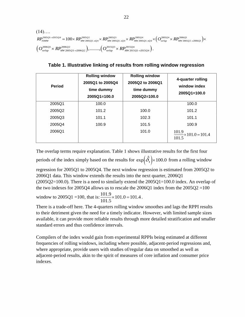
(14)….
2005 1 2015 4 2005 2 2005 3 2005 4 2005 4 2006 1
2005 1 4 2005 1 4 2005 1 4 2005 2 2006 1100
Q Q Q Q Q Q Q
TDMW MW Q Q MW Q Q MW Q Q verlap MW Q QRP RP RP RP O RP
2006 1 2006 2 2015 3 2015 4
2005 3 2006 2 2015 1 2015 4,........,
Q Q Q Q
verlap MW Q Q verlap MW Q QO RP O RP
.
Table 1. Illustrative linking of results from rolling window regression
Period
Rolling window
2005Q1 to 2005Q4
time dummy
2005Q1=100.0
Rolling window
2005Q2 to 2006Q1
time dummy
2005Q2=100.0
4-quarter rolling
window index
2005Q1=100.0
2005Q1 100.0 100.0
2005Q2 101.2 100.0 101.2
2005Q3 101.1 102.3 101.1
2005Q4 100.9 101.5 100.9
2006Q1 101.0 101.9101.0 101.4
101.5
The overlap terms require explanation. Table 1 shows illustrative results for the first four
periods of the index simply based on the results for exp 100.0 t from a rolling window
regression for 2005Q1 to 2005Q4. The next window regression is estimated from 2005Q2 to
2006Q1 data. This window extends the results into the next quarter, 2006Q1
(2005Q2=100.0). There is a need to similarly extend the 2005Q1=100.0 index. An overlap of
the two indexes for 2005Q4 allows us to rescale the 2006Q1 index from the 2005Q2 =100
window to 2005Q1 =100, that is:101.9
101.0 101.4101.5
.
There is a trade-off here. The 4-quarters rolling window smoothes and lags the RPPI results
to their detriment given the need for a timely indicator. However, with limited sample sizes
available, it can provide more reliable results through more detailed stratification and smaller
standard errors and thus confidence intervals.
Compilers of the index would gain from experimental RPPIs being estimated at different
frequencies of rolling windows, including where possible, adjacent-period regressions and,
where appropriate, provide users with studies of/regular data on smoothed as well as
adjacent-period results, akin to the spirit of measures of core inflation and consumer price
indexes.
23
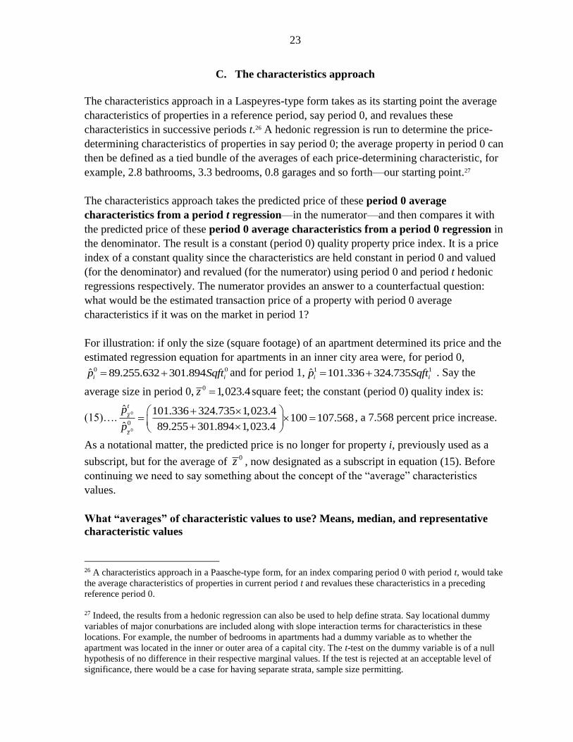
C. The characteristics approach
The characteristics approach in a Laspeyres-type form takes as its starting point the average
characteristics of properties in a reference period, say period 0, and revalues these
characteristics in successive periods t.26 A hedonic regression is run to determine the price-
determining characteristics of properties in say period 0; the average property in period 0 can
then be defined as a tied bundle of the averages of each price-determining characteristic, for
example, 2.8 bathrooms, 3.3 bedrooms, 0.8 garages and so forth—our starting point.27
The characteristics approach takes the predicted price of these period 0 average
characteristics from a period t regression—in the numerator—and then compares it with
the predicted price of these period 0 average characteristics from a period 0 regression in
the denominator. The result is a constant (period 0) quality property price index. It is a price
index of a constant quality since the characteristics are held constant in period 0 and valued
(for the denominator) and revalued (for the numerator) using period 0 and period t hedonic
regressions respectively. The numerator provides an answer to a counterfactual question:
what would be the estimated transaction price of a property with period 0 average
characteristics if it was on the market in period 1?
For illustration: if only the size (square footage) of an apartment determined its price and the
estimated regression equation for apartments in an inner city area were, for period 0,0 0ˆ 89.255.632 301.894i ip Sqft and for period 1, 1 1ˆ 101.336 324.735i ip Sqft . Say the
average size in period 0, 0 1,023.4z square feet; the constant (period 0) quality index is:
(15)….0
0
0
ˆ 101.336 324.735 1,023.4100 107.568
ˆ 89.255 301.894 1,023.4
t
z
z
p
p
, a 7.568 percent price increase.
As a notational matter, the predicted price is no longer for property i, previously used as a
subscript, but for the average of 0z , now designated as a subscript in equation (15). Before
continuing we need to say something about the concept of the “average” characteristics
values.
What “averages” of characteristic values to use? Means, median, and representative
characteristic values
26 A characteristics approach in a Paasche-type form, for an index comparing period 0 with period t, would take
the average characteristics of properties in current period t and revalues these characteristics in a preceding
reference period 0.
27 Indeed, the results from a hedonic regression can also be used to help define strata. Say locational dummy
variables of major conurbations are included along with slope interaction terms for characteristics in these
locations. For example, the number of bedrooms in apartments had a dummy variable as to whether the
apartment was located in the inner or outer area of a capital city. The t-test on the dummy variable is of a null
hypothesis of no difference in their respective marginal values. If the test is rejected at an acceptable level of
significance, there would be a case for having separate strata, sample size permitting.
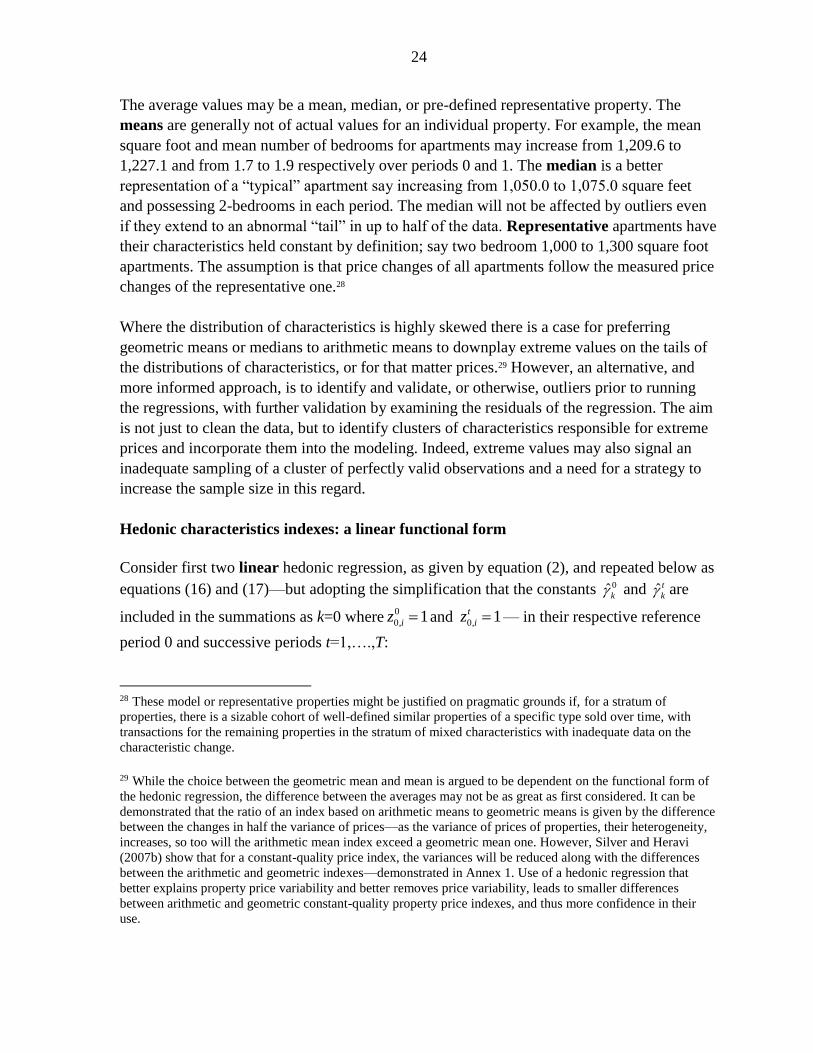
24
The average values may be a mean, median, or pre-defined representative property. The
means are generally not of actual values for an individual property. For example, the mean
square foot and mean number of bedrooms for apartments may increase from 1,209.6 to
1,227.1 and from 1.7 to 1.9 respectively over periods 0 and 1. The median is a better
representation of a “typical” apartment say increasing from 1,050.0 to 1,075.0 square feet
and possessing 2-bedrooms in each period. The median will not be affected by outliers even
if they extend to an abnormal “tail” in up to half of the data. Representative apartments have
their characteristics held constant by definition; say two bedroom 1,000 to 1,300 square foot
apartments. The assumption is that price changes of all apartments follow the measured price
changes of the representative one.28
Where the distribution of characteristics is highly skewed there is a case for preferring
geometric means or medians to arithmetic means to downplay extreme values on the tails of
the distributions of characteristics, or for that matter prices.29 However, an alternative, and
more informed approach, is to identify and validate, or otherwise, outliers prior to running
the regressions, with further validation by examining the residuals of the regression. The aim
is not just to clean the data, but to identify clusters of characteristics responsible for extreme
prices and incorporate them into the modeling. Indeed, extreme values may also signal an
inadequate sampling of a cluster of perfectly valid observations and a need for a strategy to
increase the sample size in this regard.
Hedonic characteristics indexes: a linear functional form
Consider first two linear hedonic regression, as given by equation (2), and repeated below as
equations (16) and (17)—but adopting the simplification that the constants 0ˆk and ˆ t
k are
included in the summations as k=0 where0
0, 1iz and 0, 1t
iz — in their respective reference
period 0 and successive periods t=1,….,T:
28 These model or representative properties might be justified on pragmatic grounds if, for a stratum of
properties, there is a sizable cohort of well-defined similar properties of a specific type sold over time, with
transactions for the remaining properties in the stratum of mixed characteristics with inadequate data on the
characteristic change.
29 While the choice between the geometric mean and mean is argued to be dependent on the functional form of
the hedonic regression, the difference between the averages may not be as great as first considered. It can be
demonstrated that the ratio of an index based on arithmetic means to geometric means is given by the difference
between the changes in half the variance of prices—as the variance of prices of properties, their heterogeneity,
increases, so too will the arithmetic mean index exceed a geometric mean one. However, Silver and Heravi
(2007b) show that for a constant-quality price index, the variances will be reduced along with the differences
between the arithmetic and geometric indexes—demonstrated in Annex 1. Use of a hedonic regression that
better explains property price variability and better removes price variability, leads to smaller differences
between arithmetic and geometric constant-quality property price indexes, and thus more confidence in their
use.
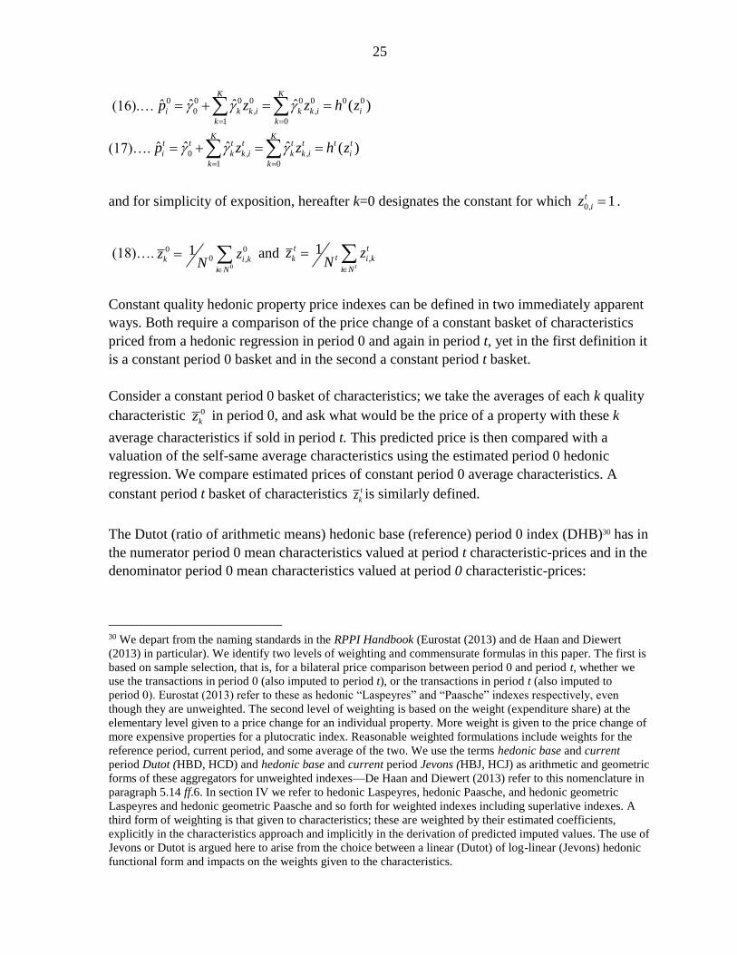
25
(16).…0 0 0 0 0 0 0 0
0 , ,
1 0
ˆ ˆ ˆˆ ( )K K
i k k i k k i i
k k
p z z h z
(17)…. 0 , ,
1 0
ˆ ˆ ˆˆ ( )K K
t t t t t t t t
i k k i k k i i
k k
p z z h z
and for simplicity of exposition, hereafter k=0 designates the constant for which 0, 1t
iz .
(18)….0
0 00 ,
1k i k
i N
z zN
and ,1
t
t ttk i k
i N
z zN
Constant quality hedonic property price indexes can be defined in two immediately apparent
ways. Both require a comparison of the price change of a constant basket of characteristics
priced from a hedonic regression in period 0 and again in period t, yet in the first definition it
is a constant period 0 basket and in the second a constant period t basket.
Consider a constant period 0 basket of characteristics; we take the averages of each k quality
characteristic 0
kz in period 0, and ask what would be the price of a property with these k
average characteristics if sold in period t. This predicted price is then compared with a
valuation of the self-same average characteristics using the estimated period 0 hedonic
regression. We compare estimated prices of constant period 0 average characteristics. A
constant period t basket of characteristics t
kz is similarly defined.
The Dutot (ratio of arithmetic means) hedonic base (reference) period 0 index (DHB)30 has in
the numerator period 0 mean characteristics valued at period t characteristic-prices and in the
denominator period 0 mean characteristics valued at period 0 characteristic-prices:
30 We depart from the naming standards in the RPPI Handbook (Eurostat (2013) and de Haan and Diewert
(2013) in particular). We identify two levels of weighting and commensurate formulas in this paper. The first is
based on sample selection, that is, for a bilateral price comparison between period 0 and period t, whether we
use the transactions in period 0 (also imputed to period t), or the transactions in period t (also imputed to
period 0). Eurostat (2013) refer to these as hedonic “Laspeyres” and “Paasche” indexes respectively, even
though they are unweighted. The second level of weighting is based on the weight (expenditure share) at the
elementary level given to a price change for an individual property. More weight is given to the price change of
more expensive properties for a plutocratic index. Reasonable weighted formulations include weights for the
reference period, current period, and some average of the two. We use the terms hedonic base and current
period Dutot (HBD, HCD) and hedonic base and current period Jevons (HBJ, HCJ) as arithmetic and geometric
forms of these aggregators for unweighted indexes—De Haan and Diewert (2013) refer to this nomenclature in
paragraph 5.14 ff.6. In section IV we refer to hedonic Laspeyres, hedonic Paasche, and hedonic geometric
Laspeyres and hedonic geometric Paasche and so forth for weighted indexes including superlative indexes. A
third form of weighting is that given to characteristics; these are weighted by their estimated coefficients,
explicitly in the characteristics approach and implicitly in the derivation of predicted imputed values. The use of
Jevons or Dutot is argued here to arise from the choice between a linear (Dutot) of log-linear (Jevons) hedonic
functional form and impacts on the weights given to the characteristics.
26
(19)….
0
00
0 0
0 0:0 0
0
ˆ
ˆk
Kt
tk kkt k
KHDB z
kk k
k
zh z
Ph zz
and a Dutot hedonic current period t quality index is defined as:
(20)….
0 0
0:0
0
ˆ
ˆtk
Kt t
t tk kkt k
K tHDC zt
kk k
k
zh z
Ph zz
If, in a perfect market, preferences change and the implicit prices of one characteristic, say an
additional bedroom, increase at an above average rate; other things being equal, utility-
maximizing buyers would substitute expenditure towards other characteristics, say more
overall space. The use of a constant period 0 characteristic basket, 0
kz would understate price
increases—the 0 0
0 0
0
ˆ
ˆ
k k
K
k k
k
z
z
expenditure weights in equation (21) do not reflect the substitution
away from characteristics with above average price increases—and of a constant period t
characteristic basket, t
kz , overstate it. This is because, as we show in section VC, the constant
quality price change of each characteristic from equations (19) and (20) are implicitly
weighted by the estimated relative values of the characteristic. For example, using the
notation in equation (15) and equations (16) and (19):
(21)….0
0
0 00
000
00 0 0 0
0 0
ˆˆˆ
ˆ ˆ
ˆ ˆ ˆ
tKKt k
t k kk kkk kz
K K
zk k k k
k k
zzp
p z z
.
For the aforementioned substitution bias relating to characteristics, a geometric mean of
equations (19) and (20)—a hedonic Fisher-type price index number—is justifiable on
grounds of economic theory, axiomatic properties, and intuition.31
31 The Consumer Price Index (CPI) Manual (ILO et al., 2004) recommends superlative price indexes—the
Fisher, Törnqvist, and Walsh indexes—as the target formulas for the higher-level indexes. These formulas
generally produce similar results, using symmetric weights based on quantity or expenditure information from
both the reference and current periods. They derive their support as superlative indexes from economic theory.
A utility function underlies the definition of (constant utility) cost of living index (COLIs) in economic theory.
Different index number formulas can be shown to correspond with different functional forms of the utility
function. Laspeyres, for example, corresponds to a highly restrictive Leontief form. The underlying functional
(continued…)
27
(22)…. 00 tt
DHF DHB DHC
z zz zP P P
The theory of hedonic regressions can be found in Rosen (1974), Triplett (1987), Feenstra
(1995)—and for an application, Silver (1999)—Diewert (2003b), and Silver (2004); the
theory of Laspeyres and Paasche bounds is in Konus (1924) and of substitution effects
warranting a (superlative) geometric mean of a Laspeyres and Paasche formula, in Diewert
(1976, 1978 and 2004).
Note that the denominator in equation (19) is the imputed or predicted price, rather than
actual price, in period 0, 0 0
k kh z , and similarly in the numerator of equation (20) we use the
imputed or predicted price rather than actual price in period t, t t
k kh z . In calculating equation
(19) we take the ratio of two imputations: the imputed price of 0
kz valued at period t
characteristic prices in the numerator and at period 0 characteristic prices in the denominator
—a dual imputation. For a linear form the average predicted price in period 0 from an
Ordinary least squares regression is equal to the average actual price, 0 0 0
k k kh z p and,
though equation (19) is hardly complex, it can be calculated with a “single imputation” as the
much simpler:
(23)…. 0
0
t
k
k
h z
p.
We return to issues of dual versus single imputation later in this section and in section IV.
Types of hedonic characteristics indexes: log-linear functional form
A constant-quality characteristics price index for a log-linear hedonic regression equation
follows similar principles: for properties i, in a given stratum, for the reference period 0 and
successive periods t=1,….,T the estimated hedonic regressions are:
(24).…0 0 0 0 0
,
0
ˆˆln ln ( )K
i k i k i
k
p z h z
forms for superlative indexes, including Fisher and Törnqvist, are flexible: they are second-order
approximations to other (twice-differentiable) homothetic forms around the same point. It is the generality of
functional forms that superlative indexes represent that allows them to accommodate substitution behavior and
be desirable indexes. The Fisher price index is also recommended on axiomatic grounds and from a fixed
quantity basket perspective (ILO et al., 2004).
(continued…)
28
(25) .… ,
0
ˆˆln ln ( )K
t t t t t
i k i k i
k
p z h z
The tilde above h denotes a log-linear functional form, the constant is included as *0
0 for
which 00, 1iz , and similarly for period t, over all observations, and periods 0 and t average
values of each k characteristic are arithmetic means:32
(26)….0
0 00 ,
1k i k
i N
z zN
and ,1
t
t
Nt t
tk i k
i N
z zN
Constant quality property price indexes can be defined in two immediately apparent ways. A
hedonic geometric Laspeyres-type constant period 0 characteristics index takes the means of
a set of characteristic 0
kz for the reference period t=0, and values them in the numerator in
equation (11) by their respective marginal valuations ˆ t
k from a log-linear hedonic
regression, estimated just from data on transacted properties in period t, and compares this
overall valuation with the same set of characteristics valued using period t=0 estimated
coefficients, that is, 0ˆk , in the denominator. The index is a ratio of geometric means with
characteristics held constant in the base (reference) period:
(27)….
0 0
ˆ00
0 0
0, 00
0ˆ 0 0:0 0 0
0 0
ˆexp ln
ˆexp ln
tk
k
k
KKt
t tk kkk kt kk
KHGMB z Kk
k kk k
zzh z h z
Pph zz z
Equation (27) holds the (quality) characteristic set constant in period 0, though a similar
index could be equally justified by valuing in each period a constant period t average quality
set. A hedonic geometric Laspeyres-type constant-period (arithmetic mean) t characteristics
index is given by:
32It is apparent from the log-linear transformation 0 1, 1 2, 2 3, 3ln ln ln ln ln lni i i i ip z z z ,
that the ,k iz , are not in logarithms and arithmetic averages of
,k iz are appropriate. The average of the
characteristics for both a linear and log-linear formulations are an arithmetic means. There is in any event an
immediate problem with taking a geometric mean of dummy variables since logarithms cannot be taken of zero
values. However, there is a work-around. Where N is the sample size, and there are n1 values of 1 and n0 of
zero, the geometric mean is 1 1 0 0
Geomean( ) Geomean( ) /n n n n N equals 1 1
Geomean( ) /n n N . Since the
1 1
Geomean( ) Arithmean( )n n for the n1 values of unity, it is quite straightforward. For example, with N=60, of
which 16 are unity, the mean is the simple proportion, 16/60=0.267.
29
(28)….
0
ˆ
0, 00
ˆ 0 0:0
0 0
ˆexp ln
ˆexp ln
tk
t
k
KKt tt
t tk k tkkt kk
K t tHGMC z Kt t k kk k k
k k
zzh z p
Ph z h zz z
Dual imputations
A natural question arises as to the phrasing of the second to last terms in equations (27) and
(28) as dual imputations, that is they use predicted (imputed) prices in both the denominator
and numerator—Silver (2001) and de Haan (2004a). As we will see in section IV, the use of
equation (28) only requires that a hedonic regression be estimated for the reference period,
that actual period prices may be used, and we lose this feature if we adopt dual imputations.
Here we explain that while there is a well-established logic for the use of dual imputations, it
need not hold in this instance, though is important in our work on weighting as explained in
section IV.
Dual imputation requires a predicted (imputed) price in both the denominator and numerator
of equations (27) and (28) as opposed to a single imputation, the last term in both equations
(27) and (28), for which 0 0 0
k k kh z p and t t t
k k kh z p . For example, in equation (27) the
single imputation hedonic approach uses the actual price in the denominator, and predicted
price in the numerator. The logic for the need for dual imputations is that the above equalities
only hold for perfectly specified hedonic regressions estimated without bias. However, this
would lead to a biased price comparison if there were substantive omitted variables in the
hedonic specification. For example, cheaper terraced houses may have no front yard (garden)
opening directly onto the street. This poorer feature would be reflected in the actual price
(denominator) of a constant period 0 index, but may be excluded or not properly represented
in the hedonic specification and thus predicted price (numerator). The numerator would be
biased upwards and index downwards. The dual imputation hedonic index would to some
extent offset an upwards bias by using predicted prices in both the numerator and
denominator. Dual imputations are generally advised for hedonic price indexes, see Silver
(2001 and 2004), de Haan (2004a), Hill and Melser (2008), Diewert, Heravi and Silver
(2009), associated comments (de Haan 2009) and response, Hill (2013) and section IV,
where we consider an alternative workaround.
Yet a feature of the OLS estimator is that the mean of actual prices is equal to the mean of
predicted prices; 0
0 0
0 0
0 0
1 1ˆ
iii
i N i N
p pN N
|z and
1 1ˆ t
it t
t t
it tii N i N
p pN N
|z. Thus the last terms in
equations (27) and (28)—see also (de Haan and Diewert, 2013, paragraph 5.38). A problem
arises, however, with the use of weights at this lower level, as explained in section IV, for
which we need dual imputations.
30
Neither a period 0 constant-characteristics index nor a period t constant-characteristic
quantity basket can be considered to be superior, both acting as bounds for their theoretical
counterparts. Some average or compromise solution is required. Diewert (1976, 1978)
defined in economic theory a class of index number to be superlative. We consider
definitions of superlative indexes in section III. This includes the Törnqvist index formula
given in this log-linear context by:
(29)….
00
ˆ
0 0
ˆ 00
00
ˆexp ln
ˆexp ln
tk
tk
k
K Kt
tk k kkTHB k k
KKz zk
kkkk
z zh z
Ph zzz
where 0 / 2t
k k kz z z
D. The imputation approach
The imputation approach differs from the characteristics approach. For the characteristics
approach the average (arithmetic mean) values of characteristics were derived in, for
example, period 0 as 3.1 bedrooms, 0.71 possession of a garage, 1,215 square feet, and then
revalued using estimated hedonic characteristic coefficients estimated from data in period t.
The characteristics approach answered a counterfactual question: what would be the price
change of a set of average period 0 characteristics valued first, at period 0 hedonic
valuations, and second, at period t hedonic valuations?
In contrast the imputation approach works at the level of individual properties, rather than the
average values of their characteristics. It tackles a similar counterfactual question: what
would a property i with its given characteristics in period 0 be worth if the same such
characteristics were revalued using period t hedonic valuations? An average of these is then
taken over the individual properties, and compared with an average of matched period 0
valuations of period 0 properties. The summation is over the predicted prices of i=1, ….,N0
period 0 properties.
The rational for the imputation approach lies in the matched model method. Consider a set of
properties transacted in period 0. We want to compare their period 0 prices with the prices of
the same matched properties in period t. In this way there is no contamination of the measure
of price change by changes in the quality-mix of properties transacted. However, the period 0
properties were not sold in period t—there is no corresponding period t price. The solution is
to impute the period t price of each period 0 property. We use a period t regression to predict
prices of properties sold in period 0 to answer the counterfactual question: what would a
property with period 0 characteristics have sold at in period t? Equation (25) provides the
answer. It is a hedonic regression using period t data, to estimate period t characteristic prices
and then apply them to period 0 characteristics values.
31
The requirements of the imputation method for a linear functional form using constant
period 0 characteristics are to: (i) estimate a hedonic regression for the reference period 0 and
each successive period t; (ii) identify the values of the characteristics of each property sold in
period 0, say property 1 had 4 bedrooms, 2 bathrooms and so forth; (iii) using the hedonic
regressions impute/predict the price of each individual period 0 property would have sold at
in periods 0 and period t; and (iv) using imputed property prices, determine the average price
of period 0 properties in period 0 and period t and as a ratio, the change in the average
period 0 constant-quality prices—the different formulations of hedonic imputation indexes
are outlined in Silver and Heravi (2007a).
Hedonic imputation indexes based on prices of individual properties i are derived from a
linear functional form and given by a Dutot (ratio of arithmetic means) index of constant
period 0 quality by:
(30)….
0
00 0
0 00 0
0
00 0
0
000 0
0,
0 0 0:0 0
0 0
ˆ1 1 ˆˆ ˆ ˆ ( )
1 1 ˆ ( )ˆ
i
ii i
i
i
t
i zt t
i z ti z i zi N i zt ii N i N
HIB zi i
i ii N
i N i N
ppp p p h zN N
Pp h z
p pN N
|
|| |
|
where 0ˆi
t
i zp|
and 0
0ˆii z
p|
are the predicted prices in periods 0 and t respectively conditioned on
(controlling for) property i’s period 0 characteristics, 0
iz .33 Note that the characteristics are
valued in the numerator and denominator at period t and 0 respectively, but the characteristic
values are held constant at period 0. Further, there is an implicit weighting given to each
property’s price change; its relative (predicted) price/value in the reference period 0, as
shown in equation (30) and considered in more detail in section VC on weighting.
Equation (31) is a Paasche-type constant period t quality index:
(31)….0,
0 0:
ˆ( )
ˆ ( )
tit
ti
tit
t
t ti zt ii N
tHDC zii z
i N
ph z
Pp h z
|
|
.
Hedonic imputation indexes for individual properties derived from a log-linear functional
form are given by Jevons (ratio of geometric means) index for a Laspeyres-type, 0iz ,
characteristics index for an individual property i:
33 Hill (2013, 890–891) reminds us that a similar bias correction to that used for the time dummy estimates
(section IIB) is required for predicted values for the imputation (and characteristics) approaches when using a
log-linear hedonic formulation, that is the addition of half the variance of the error term from the hedonic
regression (Kennedy, 1981) and Giles (2011).
32
(32)….
0
00
00
0
0
00
00
1
0
0,
1:00
0
1 ˆexp lnˆ
1 ˆexp lnˆ
ii
i
ii
tt N
i zi zt i Ni N
HJB z
N
i zi zi Ni N
ppN
P
ppN
.
The value in the numerator of equation (32) is the geometric mean of the period t price of
period 0 quantities price-determining characteristic0
,i kz . These are compared, in the
denominator, with the geometric mean of the period 0 price of the selfsame period 0
characteristics, 0
,i kz . For each property, the quantities of characteristics are held constant at0
,i kz
; only the characteristic prices change.
And a Jevons (ratio of geometric means), Paasche-type, constant period t characteristics,tiz ,
is given by:
(33)….
1
,,
1
00
,,
1 ˆexp lnˆ
1 ˆexp lnˆ
t
ttii tt
t
ttii tt
tt Nt i zi z
i NJ i NHIP
Nt i zi z
i Ni N
ppN
P
ppN
E. An indirect approach to hedonic price indexes
The indirect approach is not new. The literature on its properties and application include
Feenstra (1995), Silver and Heravi (2001), Diewert (2003a), Pakes (2003), Triplett (2006),
Heravi and Silver (2009), and de Haan and Diewert (2013). Consider the change in
arithmetic mean prices phrased as actual or, for an OLS regression, predicted prices:34
(34)….
0
0 0
0 0
0 0
1 1ˆ
1 1ˆ
t ti i
t t
i
t t
t ti z i zi N i N
i i zi N i N
p pN N
P
p pN N
| |
|
and as a ratio of geometric mean prices:
34 Note that we use the ratio of average predicted prices which, from an OLS regression, equals the ratio of
average actual prices. Our use of predicted prices is to enable terms in equations (34) and (35) to more
obviously cancel, as we proceed.
33
(35)….0 0
0
0 0 0
0 0
1 1
1 1
00 0 0
1ˆ ˆexp ln
1ˆexp ln
ˆ
t t
t t ti i it t t
i
i i
N Nt t t
ti z i z i zi N i N i N
N N
i zi z i z i N
i N i N
p p pN
P
pp p N
| | |
|| |
Equations (34) and (35) are measures of the change in average price, not constant–quality
price change. The tN properties transacted in period t may well have quite different
characteristics than the 0N properties transacted in period 0. The measure of the change in
prices of properties transacted is contaminated by changes in the quality-mix of properties
sold.35 In this indirect approach the change in the average price of properties transacted given
in equations (34) and (35)—the raw average price change, P —is divided by (adjusted for)
the volume change, qualV , in the quality of transacted houses between the two periods to
obtain a constant-quality price index, that is: 36
(36)…. const qual qualityP P V .
Consider a linear hedonic regression and characteristics (quality) volume index where, in
equation (37), the arithmetic means of the volume of characteristics change from 0
kz in period
0 in the denominator to t
kz in period t in the numerator. However, the estimated
characteristics’ valuations are held constant, in this case in period 0, 0ˆk , as can be seen from
both the characteristics and imputation approaches:
(37)…..
0
0
000
0
0 0 0 00
00
1ˆˆ
1ˆˆ
ti
t
i
ttk k t i z
k kqual k i N
k k k ki zk
i N
pzh zN
Vz h zp
N
|
|
Using equation (37) and the feature of an OLS regression, that the mean of predicted ‘left
hand side’ values equals the mean of their actual values:
35 It may be that a few properties are sold in both periods, for which a sub-index based on matched actual prices
can be calculated, and weighted into an overall index. Even then, these properties may have
improved/deteriorated between the two periods, sometimes with major renovations such as the addition of
bedrooms, bathrooms, finishing of basements.
36 In national accounting changes in nominal values are decomposed into price changes and volume changes
(2008 SNA, chapter 15). The latter includes changes in the quality of what is produced/consumed. If, for
example, the nominal values of houses transacted increased, on average, by 10 percent, the number of houses
sold increased by 5 percent, the quality of houses sold increased by 1 percent, then the price change is equal to
the nominal value change of 1.10 divided by the volume change (1.05 times 1.01) which equals 1.03725, a
3.725 percent increase. Changes in average property prices already reflect an adjustment for the change in the
number of houses sold.
34
(38)…. 0
0 0
0 0
0 0
1 1ˆ
iii
i N i N
p pN N
|z and
1 1ˆ t
it t
t t
it tii N i N
p pN N
|z
and adopting the hedonic imputation approach, an indirect constant period t characteristics
price index is:
(39)….
0
0 0
0
0 0 0
0 0
11 1ˆˆ
1 1 1ˆ ˆ
ttii tt t
ti it
tt
i tt t i zi zconst qual i Ni N i N
i ti z i zi N i N i N
pp pNN N
P
p p pN N N
||
| |
or equivalently, phrased as a hedonic characteristics index, again using equation (38), the
indirect constant period t characteristics price index is:
(40)….
0
0 0
0 0
0 0
0 0 0 00 0
0 00 0
1 1ˆˆ ˆ
1 1ˆ ˆˆ
ti
t t
i
t tt t
i k k k kt t i zconst qual i N k i N k
k k k ki i zk k
i N i N
p pz zN N
Pz z
p pN N
|
|
0
00 0
0 0 0 0 0 0
0 0 0
ˆˆ ˆ
ˆ ˆ ˆ
t tt t tt tk kk k k kk kkk k
t tk k k k k k k k
k k k
zz zh z
z z z h z
For example, if larger properties, with more bedrooms, having garages and so forth were
selling in period t as opposed to period 0, then the qualV index in equation (37) would
increase as the mean quantities of characteristics in equation (38) increased from 0
kz to t
kz ,
each valued by its estimated marginal values in period 0. Since the numerator, P , is the
change in average prices calculated from the sample of properties sold in period t, ti N ,
compared with period 0, 0i N , the final terms in equations (39) and (40), const qualP , are
measures of price change adjusted for changes in the quality-mix of properties transacted.
Note that the resulting indirect indexes in equations (39) and (40) are hedonic current
period t valued (weighted) index, though constant period 0 characteristics price indexes can
be similarly defined.37
37 A well-established feature of Laspeyres and Paasche is that they jointly pass the factor reversal test, that is:
the product of a Laspeyres price (quantity) and Paasche quantity (price) index is equal to an index of the change
in value, Diewert (2004, chapter 16). In equations (39) and (40) the change in average monetary value was
divided by a Laspeyres-type quality volume index to result in a hedonic current period price index.
35
and in log-linear form:
(41)….
0
0
0
0
0 00
00
1 ˆˆexp ln exp ln
1 ˆˆ exp lnexp ln
tit
i
t t
k kt i zconst qual i N k
k ki zki N
p zN
P
zpN
|
|
0
00
0
ˆexp ln
.ˆexp ln
t tt tk kk kk
tt k kk k
k
zh z
h zz
In calculating equation (41) we take the change in average prices in the numerator and divide
it by the volume change in average characteristics, from 0
kz to t
kz , holding the marginal
valuations of these average characteristics constant in period 0, 0ˆk . This yields a constant-
quality characteristics price index with quality characteristics held constant at current period
values, t
kz .
F. Arithmetic versus geometric aggregation: how much does it matter?
On the importance of a geometric versus an arithmetic hedonic formulation
Throughout this exposition the distinction between an arithmetic mean and geometric mean
of constant-quality price changes has been emphasized. Its impact is going to be an empirical
matter which will vary from country to country, and region and type of property within a
country. In this section we consider the differences in the aggregation formulas: arithmetic
versus geometric means.
Much of this paper has been concerned with outlining the paths of aggregation for a linear
hedonic regression using an arithmetic aggregation and log-linear hedonic regression using a
geometric aggregation. There are questions as to how much the functional form of the
aggregator, linear (Dutot) versus geometric (Jevons) matters, what are the factors
determining the magnitude of the difference between a hedonic Jevons and hedonic Dutot
indexes, and mechanisms for further minimizing the difference? The difference between
hedonic unweighted indexes was developed by Silver and Heravi (2007b) and integrated into
the sampling and axiomatic approaches to index number theory.
36
Dutot’s failure of the units of measurement (commensurability) test
In consumer price index number theory, the Jevons index is superior to the Dutot index, on
axiomatic grounds (Diewert, 2004, chapter 16). The Dutot index fails the units of
measurement (commensurability) test,38 which Jevons passes;39 has an arbitrary element that
depends on the units of measurement. The recommendation is that Dutot should only be
applied to heterogeneous goods and services, something that properties are not:
“Under these circumstances [heterogeneous items], it is important that the elementary index
satisfies the commensurability test, since the units of measurement of the heterogeneous
items are arbitrary, and hence the price statistician can change the index simply by changing
the units of measurement for some of the items.” (Diewert (2004, chapter 20 paragraph
20.65, Consumer Price Index Manual).
However, as was shown in section II, a special feature of an imputation property price index
is that price changes are aggregated across individual properties. The Dutot index number
formula implicitly weights individual property price changes, i , by their relative prices in the
reference period, 0
0
, ii zw , and these relative prices of individual properties are synonymous with
the relative values of each property:
(42)….
0
00
0 0 00
0
00 0 0
0 0
, 0
0 ,,
, , 0
0 0 0 ,
, , ,
ˆˆˆ ˆ ˆ
ˆ ˆ ˆ
i
ii
i i
i
i i i
t
i zt
ti zi z
i N i z i zi N
i zi Ni z i z i z
i N i N
ppp p p
wp p p
.
The Dutot index in this context is a value-weighted index of individual property price
changes. Frisch (1930, page 400) shows that a general condition that the commensurability
test is satisfied is that, as in equation (42), it can be phrased as a value weighted average of
price changes. Thus in the context of using the formula for property price indexes for
individual properties, its failure of the commensurability test is not an issue.
We note that the failure of the commensurability test is not mitigated by the quality
adjustment. The units of measurement of properties while originally diverse, say some
38 The commensurability test requires that the index number shall be unaffected by a change in units of
measurement; that is, if for any commodity the price, p, is replaced by p and at the same time the quantity q is
replaced by /q both at the time 0 and at the time 1, then the price index between periods 0 and t shall remain
unchanged, regardless of the value of .
39 Diewert (2004, chapter 20 paragraph 20.68) notes in the Consumer Price Index Manual that “If there are
heterogeneous items in the elementary aggregate, this is a rather serious failure and hence price statisticians
should be careful in using this [Dutot] index under these conditions.”
37
properties of differing sizes, number of bedrooms and so forth, have as an intention of the
hedonic adjustment that each of the price changes are of properties of similar
characteristics—a constant quality index. This might be achieved without essentially any
change to each property’s period 0 characteristics. The price change of an individual property
i, is measured by 0 0
0ˆ ˆi i
t
i z i zp p| |
; that is, the counterfactual predicted prices in period t of period 0
characteristics, 0ˆi
t
i zp|
are compared with the predicted prices in period 0 of the self-same period
0 characteristics, 0
0ˆii z
p|
. The hedonic standardization of units is for each property over time,
rather than across properties in a single period, as would be meaningful for the
commensurability test.
Similarly, for a constant period t quality, the hedonic adjustment is applied to ensure the
price change is of constant quality, that is:
(43)….
1
10
0
0
ˆ ˆ
ˆ ˆˆ
ˆ
t ti it t
tti
t i
tit t
i
t t
i z i zi N i N
ti z
i zi N
i zi N i z
p p
p pp
p
| |
| |
|
|
There is little a priori reason to expect there to be less variance, and thus more similar units
of measurement, in the period 0 predicted prices of the sample of ti N characteristics, than
the period 0 predicted prices of the sample of 0i N characteristics.
So commensurability is not an issue. This is an important matter since we can argue that the
choice between using a linear/arithmetic formulation as opposed to a log-linear/geometric
formulation can be determined by the appropriateness of the functional form of the hedonic
regression, as opposed to the axiomatic failings, or otherwise, of the aggregation formulas.
So what determines the difference between hedonic Dutot and Jevons and when will it
be minimal?
First, a second-order approximation to the relationship between the Dutot and Jevons
indexes—without constant quality hedonic adjustments—has been defined by Diewert
(1995a; 2002c; and 2004, chapter 20), Dalen (1992), Balk (2005 and 2008), and Silver and
Heravi (2007b)—also Annex B of this paper. The Dutot index, DI , is equal to the Jevons
index multiplied by the change in the variances of prices, terms of the difference in the
variances of log-prices between periods 0 and t, terms of the difference in the variances of
log-prices between periods 0 and t, 2 2
0t :
38
(44)….
2
2 2
00 2
0
exp / 2exp / 2
exp / 2
ttD J J
tI I I
Note that the variances might be considerable, but it is their change that matters. It is
apparent that as property heterogeneity and price dispersion decrease, so too will the
difference between the two indexes. Since the variance of prices, as a measure, is specific to
the mean, as property price inflation falls, so too is the likelihood that the variances will fall,
and vice versa—a positive relationship between inflation and its dispersion (Friedman, 1977,
Balk, 1983, Reinsdorf, 1991, and Silver, 2001)—and, thus, the difference between the two
formulas. The differences can readily be numerically ascertained by compilers of property
price indexes by simply using both formulas. For property price indexes, a calculation
routine for summing the price observations for a Dutot index simply has to be modified to
sum the logarithms of prices, and take the exponent of the total, for the Jevons index.
However, our concern is with hedonic-adjusted versions of these formulas. Silver and Heravi
(2007b) extend the above analysis to indexes that control for observable product
heterogeneity through hedonic regressions. The comparison of quality adjusted prices
removes some of the quality heterogeneity of the properties making the use of a
heterogeneity-controlled Dutot more acceptable. The relationship between a heterogeneity-
controlled Dutot and Jevons is given by:
(45)…. * 2 2 * 2 2
1 0 0ˆˆ exp exp / 2 exp / 2D t J tP P
.
where the * denotes heterogeneity-controlled and where 2
, for 0,t , are the variances of
the residuals of observations from a hedonic regression in periods 0 and t respectively. Thus
the difference between the Jevons and the Dutot hedonic price index is related to the change
in the variance of the residuals over time. Assuming 2 2 2 2
0 0t t (from (39) and
(40) respectively) then the discrepancy between the Jevons and Dutot indices in (39) will be
greater than the discrepancy between the heterogeneity-controlled Jevons and Dutot indexes
in (40). Note that the difference between *
JP and *
DP is reduced as, first, for 0,t , 2 0 ,
and second, for 2 2 2 2
0 0t t , if the hedonic regression controls for the same
proportion of price variation in each period, that is 2 2
for 0,t where Annex B
provides details.
Of note is that hedonic imputation and characteristics indexes are considered in section IV
for cases where there are sparse data in thin markets. In these cases, the robust periodic
re-estimation of hedonic regression equations in each period may be considered infeasible.
The use of a single reference period hedonic regression, advocated in this section, is less
39
likely to suffer from changes in 2 2
0t due to changes in the specification and fit of the
regression.40
In the next section we continue the focus on hedonic base and current period index number
formulas, but consolidate and narrow down the options. The myriad options considered here
arise from having formulas from (i) three direct approaches and an indirect one; (ii) for each
approach, two different functional forms for the hedonic regression; (iii) commensurate
arithmetic and geometric formula; (iv) different periods at which quantities (and for the
indirect method prices), are held constant; and (v) the use or otherwise of dual imputation.
First, to help consolidate these approaches, we look at equivalences, then at weighting
systems, and then formulate target indexes. This is followed by a practical consideration of
working in thin markets with sparse data and a concern with periodic hedonic regression
estimation.
III. SOME EQUIVALENCES
The three approaches have quite different, yet quite valid, intuitions. We show here that (i)
the characteristics and imputations approaches yield the same answer under the quite credible
conditions of using either a linear or log-linear functional form as long as arithmetic means
are taken of characteristics/imputed prices; (ii) reiterate that for these formulations, the
indirect approach to each, as shown above, is equal to the direct approach; and (iii) show the
time dummy to have the same intuition as the indirect approach and outline the conditions for
the equivalence of the time dummy and imputation/characteristics approaches. It is argued
that there is an axiomatic sense in which the equality of results from quite different intuitions
argues well for these formulations.
When imputation index equals characteristics index
For a linear functional form the characteristics and imputation approaches give the same
answer if, (i) for the characteristics approach, 0
kz and t
kz are arithmetic means of characteristic
values and (ii) for the imputation approach, the ratio of average predicted prices is a ratio of
arithmetic means. An index with characteristics held constant in the reference period 0 is
given by:41
40 Further, de Gregorio (2012) has shown that that the effectiveness of stratified sample designs can reduce the
source of discrepancies between the Dutot and Jevons index number formulas.
41 Since 1 1 1 1
J JK K
ij ji
i j j i
a a
.
40
(46)….0 0
0 0
00 0 0 0
0
00
00 0
0 00
, ,
0 00
00 0 00 0
,,
0 00
1 1
1 1
ˆ ˆ ˆˆˆ
ˆ ˆ ˆˆ ˆ
ik
ki
K KKt t tt
t k i k k k ik k i zzDHIB k kk i N i N i N
K KKztt
zk k k k ik i k i z
k kk i Ni N i N
N N
N N
z z pzpP
p z zz p
and characteristics held constant in the current period t by:
(47)…. 0
, ,
0 00
00 0
,,
0 00
1 1
1 1
ˆ ˆ ˆˆˆ
ˆ ˆ ˆˆ ˆ
t t
t t
tit t t t
k
tk t
itt t
K KKt t t t tt t
t k i k k i kk k i zzDHIB k kk i N i N i N
K KKzt t tt t
zk k k i kk i k i z
k kk i Ni N i N
N N
N N
z z pzpP
p z zz p
The equivalences also holds when equations (46) and (47) are phrased as weighted price
changes whereby the weight given to the price change of a characteristic 0
ˆ
ˆ
t
k
k
is the relative
value of that characteristics in the reference period, 0 0
0 0
0
ˆ
ˆ
k k
K
k k
k
z
z
and the index is a weighted
arithmetic mean of price changes,
0 0
00
0 0
0
ˆˆ
ˆ
ˆ
tKk
k k
k k
K
k k
k
z
z
. For example, for the period 0 characteristic
index in equation (46):
(48)….
0
00
00 00
0
0 00
0 0
00 0000
00
0 000 0 0 0
0 0
ˆˆ ˆˆ ˆˆˆ ˆˆ
ˆ ˆˆ ˆ ˆ
i
ii
k i
i ik
ttKK i zk tt
t i zk kk k i zi Nkz i zDHB kk i N
K Kz
i z i zzk k k k
i N i Nk k
ppz pzp p
Pp pp z z
For a log-linear functional form the characteristics and imputation approaches give the
same answer if, (i) for the characteristics approach, 0
kz and t
kz are arithmetic means of
characteristic values and (ii) for the imputation approach, the ratio of average predicted
prices is a ratio of geometric means. A similar result is given in Hill and Melser (2008) and
Hill (2013) though they confine the equivalence to the log-linear (semilog) hedonic model:
“T3 [a geometric mean of a Geometric Laspeyres and geometric Paasche hedonic
indexes] … has attractive properties when the hedonic takes the semilog form. The
fact that it can be defined in either goods or characteristics space adds flexibility to
t6he way the results can be interpreted. For example, T3 can be interpreted either as
measuring the average of the ratios over the two region-periods of the imputed price
41
of each house or as the ratio of the imputed price of the average house. Which
perspective is most useful may depend on the context.” Hill and Melser (2008, page
602).
An index with characteristics held constant in the reference period 0 is given by:
(49)….
0
0
0
0 0
0 0
0
0
00
,
000
00 0 0 0 0
,0 0 0
1
1
ˆˆˆ exp lnexp lnˆ
ˆ ˆ ˆ ˆexp ln exp ln
k
k
k
k
KKK zttt
t i k kk kkz kDHIB k i Nk
Kz z K K
zk k k i k k
k k k i N
N
N
zzp
Pp
z z
0
0
0
0
0 0
0
0
0 0
1
0
,
0
1
0 0 0,
0
1
1
ˆexp ln ˆ
ˆexp ln ˆ
i
i
Kt t N
k i k i zki N i N
KN
k i k i zki N i N
N
N
z p
z p
and characteristics held constant in the current period t by:
(50)….
0
,
000
00 0 0
,0 0 0
1
1
ˆˆˆ exp lnexp lnˆ
ˆ ˆ ˆ ˆexp ln exp ln
t
t
tk
t tk
tk
tk
t
KKK zt tt tt
t i k kk kkz kDHIB k i Nk
Kz z K Kt tz
k k k i k kk k k i N
N
N
zzp
Pp
z z
1
,
0
1
0 0,
0
1
1
ˆexp ln ˆ
ˆexp ln ˆ
t
t
t
tit t
t
tit t
Kt t t Nk i k i z
ki N i N
Kt Nk i k i z
ki N i N
N
N
z p
z p
.
While we stress the importance of using arithmetic means for the linear and log-linear
hedonic functional forms, we note that it is straightforward to demonstrate that geometric
means of characteristic values have equivalences for imputation and characteristics
approaches for a
log-log (double-logarithmic) hedonic functional form (though see section IIA on limitations
of use of this form for hedonic regressions).
The imputations and characteristics approaches both have an intuition: the former as a ratio
of average constant price changes of matched properties, and the latter as a ratio of prices of
a constant-quality basket of characteristics. That the two approaches yield the same answer is
an important factor in the selection of a credible formula.
42
Further, this section on equivalences consolidates the choice of methods and allows further
work on weighting to be written in the quiet confidence that when using the imputation
approach as a more natural vehicle for developing weights, corresponding results apply for
the characteristics approach.
Additivity
Moreover, the formulas are additive in the sense that as the arithmetic mean of characteristics
of properties can extended to include more properties, say a merger of two stratum 1s and 2s
of sizes 1n and 2n respectively, where 1 2n n N . The imputation approach using a weighted
arithmetic means of characteristics of both strata, will give the same result as the
characteristics approach using the arithmetic mean of the two strata combined.
(51)….
1 21&2
1 2
1&21 2
1 2
1 2
1 2
0
0
0
0
0
, ,
0 00, 0
0:0 0
, ,00 0
ˆ ˆˆ ˆ
ˆ ˆˆ ˆ
is s
i
i
s s
K K Kt s t st t sk i k k i k k ki z
k kt i N i N i N k
KHDB z K Kt ss s
i zk kk i k k i ki N
kk ki N i N
n nz zp z
N NP
n np zz zN N
|
|
That the indirect imputation/characteristics approach is equivalent to the direct
imputation/characteristics approach
Equations (39) to (41) show the direct and indirect approaches yield the same result. For
example, equation (40) for a linear functional form of an indirect hedonic property price
index that holds characteristics constant in period t is given by:
(52)….
0
0
0
0 00
0 0
1ˆ
1 ˆ
t
t t
i k ktconst qual i N k
k ki k
i N
p zN
Pz
pN
=0
0 00 0
0 0 0
0
0 0 0
0
1
1 1
11ˆˆ ˆ
1ˆ ˆ ˆ
tt tii i tt t
ti i i
tt
tt i zi z i zi Ni N i N
i z i z i zi N i N i N
N
N N
pp pNN
p p pN
.
Similarly, for a log-linear hedonic regression and a geometric-current period t hedonic
characteristics index, using equations (41):
43
(53)….
0
,
00
0 0 00
,0 0
1 ˆˆ ˆexp ln exp ln
1ˆ ˆˆ exp lnexp ln
tk
tit
tk
ti
t
K zt tt
i k ktk i zconst qual i N kk
K z
k i k kt i zk ki N
p zN
P
zpN
|
|
1
0
,
00 0
10 0 0 0 0 0
, ,
0 0 0
ˆˆ ˆ ˆexp lnexp ln exp ln
ˆ ˆ ˆexp ln exp ln exp ln ˆ
t
ti
t
t
ti
t
KKt tt t t t Nk kk k i k k i z
kk k i N
Kt N
k k i k k i k ki z
k k k i N
zz z p
z z z p
.
Equation (53) can be written in a more intuitively appealing way as the change in average
price divided by the change in the volume of average characteristics, each characteristic
being valued by its estimated hedonic characteristic marginal value.
(54)…. 0
0
1
0
10
0
1
ˆexp ln
1
t
t
N
t
it
const qual t ti N
k k kNk
t
i
i N
pN
P z z
pN
The above formulas weight each price equally. The needs of a plutocratic index are that price
changes be weighted by the relative value of the transactions (see Rambaldi and Rao (2013)
for details of a democratic index).
IV. WEIGHTS AND SUPERLATIVE HEDONIC PRICE INDEXES
So far we have made no mention of an essential element of index number construction: the
weighting of price changes. If one index number formula has a superior weighting, other
things being equal, it is preferred. As noted by Griliches (1971, page 326): “There is no good
argument except simplicity for the one-vote-per-model approach to regression analysis.”42
We distinguish between two levels of aggregation: the lower and higher levels. Property
price indexes are often stratified by type and location to form more homogeneous strata of
42 Griliches (1961, 1964), Adelman and Griliches (1961) revived the hedonic approach to the construction of
price indexes. Griliches (1971) raised methodological issues that foreshadowed many of the issues of concern in
this paper including the need for weighting in regression estimates and the empirical form of the relationship,
commenting on the preferred use of semi-logarithmic form.
(continued…)
44
properties, say apartments in the downtown area of a capital city.43 At the lower or
elementary level constant-quality price indexes are estimated for each stratum. The national
or some higher-level index is compiled as a weighted average of the constant-quality price
changes of the individual strata indexes.
The higher-level weights can be the relative values of transactions or stocks of properties for
each stratum.44 This choice between the use of “transactions” or “stocks” as weights depends
on the purpose of the property price index and availability of adequate data on the stock of
properties. Fenwick (2013) outlines issues relevant to such a choice, the concern here being
with the incorporation of weights, implicitly or explicitly, into the lower level within stratum
measured constant-quality property price index.
There is a literature on elementary price index number formulas based on the needs of
consumer, producer and trade price indexes. While some of these results have a bearing on
the analysis here, the context differs in two important respects. First, the matched prices are
predicted constant-quality prices for individual properties. The transaction quantity to be
assigned to each price is unity. Second, the elementary property price indexes are constant-
quality indexes that make use of hedonic (or repeat sales) regressions. The weights given to
the property price observations, for a time dummy method, are implicit in the way
observations of prices enter into the regression or aggregation formula. We provide an
improved mechanism for weighting at this lower elementary level.45
In this section we consider three issues which allow us to develop a hedonic superlative price
index number: a proposed method for weighting hedonic property price indexes to form
quasi-superlative indexes for both the linear/arithmetic (section A) and log-linear/geometric
(section B) formulations; since sections A and B are concerned with quasi-superlative
hedonic indexes we say something in section C about our understanding of substitution bias
in this context. In section D we define hedonic superlative price indexes and show how they
differ from the “quasi” formulations in terms of an absence of sample selectivity bias. This
formulation differs from accepted wisdom and in section E we use, the in many ways seminal
paper by, Hill and Melser (2008) to show how this formulation improves on the one they
advocate, one used by others in much subsequent work. The discussion in sections A to E is
43 It is well established in sampling theory (Cochran 1977) and its application to price indexes that stratification
can lead to large reductions in sampling error, see Dalèn and Ohlsson (1995) and Dorfman et al. (2006). There
are trade-offs. A finer classification results in more similar houses—that is, each stratum has more
homogeneous properties—and better estimates of quality-mix change. However, the resulting sample size of
transactions in each stratum will be relatively small and estimates of the constant-quality price change
inefficient—have relatively wide confidence intervals. A relatively coarse stratum classification will lead to
efficient estimates of constant-quality price indexes, but ones based on a restrictive assumption that the
coefficients for quality attributes across the many strata now included, are the same. 44 Rambaldi and Rao (2013, 14–17) provide details on hedonic price indexes using democratic (equal) weights
as opposed to plutocratic (stock or expenditure-share) weights.
45 The author is currently working on weighting systems at the higher level.
45
concerned with the hedonic imputation approach as a natural framework to use to incorporate
explicit weighting but, as demonstrated by Hill and Melser (2008), has an equivalence to the
characteristics approach. In section F we turn to the time dummy approach and methods for
introducing weights. In spite of (again seminal) work by Diewert (2005a) we find the
hedonic imputation approach a more natural method and outline our concerns about
introducing weights into the time dummy approach. Finally, in section G we consider the
adoption of stock, as opposed to transaction value, weights.
A. Lower-level weights for a linear/arithmetic hedonic formulation
Say there is transaction price for a property in the reference period, but not in the current
period. We want to estimate the constant-quality price change of the property. The property’s
matched current period price is estimated as the predicted price in the current period t of the
property using its period 0 characteristics. Given a hedonic regression is run in each over all
properties transacted in period t, then the counterfactual period t predicted price of an
individual property i with k characteristics whose values are0
,i kz in period 0 can be estimated
as 0ˆi
t
i zp
. (For ease of exposition we drop the k subscript in subsequent algebra: 0
iz refers to the
values of all individual characteristics in the hedonic regression). If, for example, a detached
property with 4 bedrooms in a particular postcode, 3 bathrooms, a floor area of 3,000 square
feet, and so forth, is sold in period 0 for 750,000, we can use a hedonic regression estimated
in period t to answer a question as to the estimated price of a property with the same period 0
characteristics sold in period t. By comparing the average price in period 0 with the average
predicted price in period t of properties with the same period 0 characteristics, we have a
measure of constant quality price change. This is the hedonic imputation approach, which we
focus on since it is a more natural form to consider issues of weights given to each matched
property price transaction. Its equivalence to the characteristics approach, for these
formulations, was established in section III though we return to this issue later.
Consider the hedonic imputation Dutot index in equation (42): a simple ratio of (constant
period 0 quality) arithmetic mean prices of properties sold in period 0. The denominator is
the average actual prices of properties transacted in period 0 and the numerator is the average
(by definition, counterfactual) predicted price in period t of period 0 properties:
(55)….0
0
0 0
0 00
0 00 00
0
0 0
0 00
0 0
0 0
0,
0 0:0
1
1
ˆ ˆˆ ˆˆ ˆ ˆ
ˆ ˆˆ
i i
i ii
i i
i
i i
t t
i z i zt
i z i zi z i N i Ni z i zt i N
HDB z
i z i zi
i N i Ni N
N
N
p pp pp p p
Pp p
p
since for OLS: 0 0
0 0
0 0
0 01 1ˆ
i ii z i zi N i NN N
p p
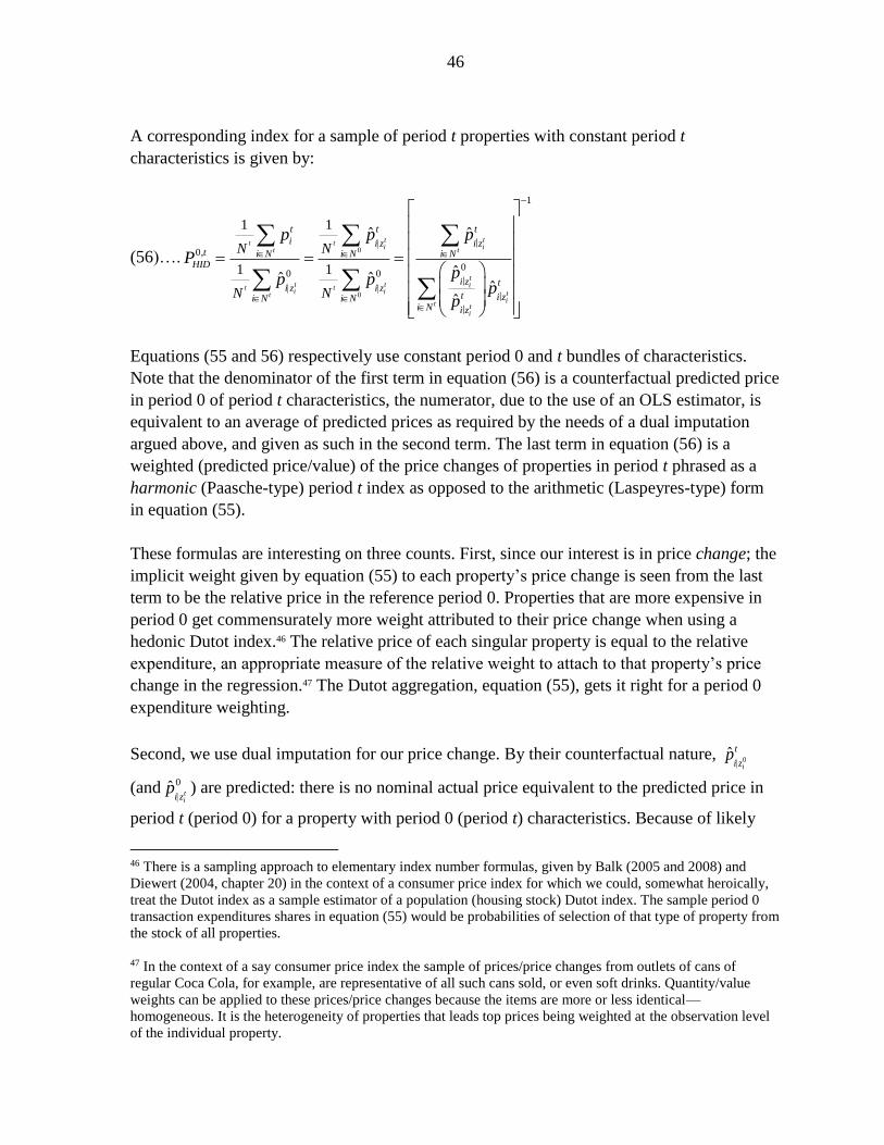
46
A corresponding index for a sample of period t properties with constant period t
characteristics is given by:
(56)….0
0
1
0,
00 0
1 1
1 1
ˆ ˆ
ˆˆ ˆˆ
ˆ
t t
t t
t ti it t
tt t ii i tt
it t
i
t t t
i i z i zt i N i N i N
HID
i z ti z i z
t i zi N i Ni N i z
N N
N N
p p p
Ppp p
pp
|
|
|
|
Equations (55 and 56) respectively use constant period 0 and t bundles of characteristics.
Note that the denominator of the first term in equation (56) is a counterfactual predicted price
in period 0 of period t characteristics, the numerator, due to the use of an OLS estimator, is
equivalent to an average of predicted prices as required by the needs of a dual imputation
argued above, and given as such in the second term. The last term in equation (56) is a
weighted (predicted price/value) of the price changes of properties in period t phrased as a
harmonic (Paasche-type) period t index as opposed to the arithmetic (Laspeyres-type) form
in equation (55).
These formulas are interesting on three counts. First, since our interest is in price change; the
implicit weight given by equation (55) to each property’s price change is seen from the last
term to be the relative price in the reference period 0. Properties that are more expensive in
period 0 get commensurately more weight attributed to their price change when using a
hedonic Dutot index.46 The relative price of each singular property is equal to the relative
expenditure, an appropriate measure of the relative weight to attach to that property’s price
change in the regression.47 The Dutot aggregation, equation (55), gets it right for a period 0
expenditure weighting.
Second, we use dual imputation for our price change. By their counterfactual nature, 0ˆi
t
i zp
(and 0ˆ tii z
p
) are predicted: there is no nominal actual price equivalent to the predicted price in
period t (period 0) for a property with period 0 (period t) characteristics. Because of likely
46 There is a sampling approach to elementary index number formulas, given by Balk (2005 and 2008) and
Diewert (2004, chapter 20) in the context of a consumer price index for which we could, somewhat heroically,
treat the Dutot index as a sample estimator of a population (housing stock) Dutot index. The sample period 0
transaction expenditures shares in equation (55) would be probabilities of selection of that type of property from
the stock of all properties.
47 In the context of a say consumer price index the sample of prices/price changes from outlets of cans of
regular Coca Cola, for example, are representative of all such cans sold, or even soft drinks. Quantity/value
weights can be applied to these prices/price changes because the items are more or less identical—
homogeneous. It is the heterogeneity of properties that leads top prices being weighted at the observation level
of the individual property.
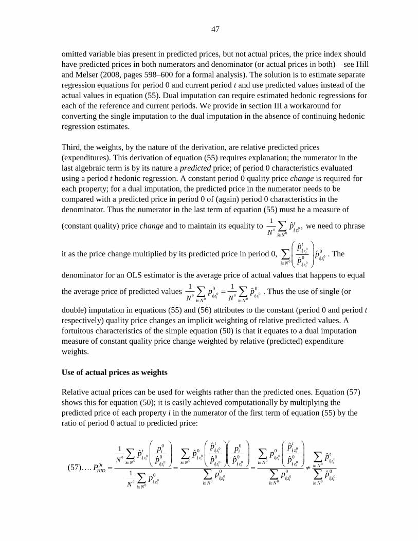
47
omitted variable bias present in predicted prices, but not actual prices, the price index should
have predicted prices in both numerators and denominator (or actual prices in both)—see Hill
and Melser (2008, pages 598–600 for a formal analysis). The solution is to estimate separate
regression equations for period 0 and current period t and use predicted values instead of the
actual values in equation (55). Dual imputation can require estimated hedonic regressions for
each of the reference and current periods. We provide in section III a workaround for
converting the single imputation to the dual imputation in the absence of continuing hedonic
regression estimates.
Third, the weights, by the nature of the derivation, are relative predicted prices
(expenditures). This derivation of equation (55) requires explanation; the numerator in the
last algebraic term is by its nature a predicted price; of period 0 characteristics evaluated
using a period t hedonic regression. A constant period 0 quality price change is required for
each property; for a dual imputation, the predicted price in the numerator needs to be
compared with a predicted price in period 0 of (again) period 0 characteristics in the
denominator. Thus the numerator in the last term of equation (55) must be a measure of
(constant quality) price change and to maintain its equality to 0
0
0
1ˆ ,
i
t
i zi NN
p
we need to phrase
it as the price change multiplied by its predicted price in period 0, 0
0
0 0
0
0
ˆˆ
ˆi
i
i
t
i z
i zi N i z
pp
p
. The
denominator for an OLS estimator is the average price of actual values that happens to equal
the average price of predicted values 0 0
0 0
0 0
0 01 1ˆ
i ii z i zi N i NN N
p p
. Thus the use of single (or
double) imputation in equations (55) and (56) attributes to the constant (period 0 and period t
respectively) quality price changes an implicit weighting of relative predicted values. A
fortuitous characteristics of the simple equation (50) is that it equates to a dual imputation
measure of constant quality price change weighted by relative (predicted) expenditure
weights.
Use of actual prices as weights
Relative actual prices can be used for weights rather than the predicted ones. Equation (57)
shows this for equation (50); it is easily achieved computationally by multiplying the
predicted price of each property i in the numerator of the first term of equation (55) by the
ratio of period 0 actual to predicted price:
(57)….
0
0
0 0
0 0 00
0 0 00 0 0 00
0 0 00 0 0
0
0 00 0
0 0 0 0
0
0 0 00
1
1
ˆ ˆˆ ˆ ˆˆ ˆ ˆ ˆ
ˆ
i i
i i ii
i i i i
i i ii
t t
i z i zt i it
i z i z i zi zi N i N i Ni z i z i z i zt i N
HID
i z i z i zi z i N i N i N
i N
N
N
p pp pp p p pp p p p
Pp p p
p
0
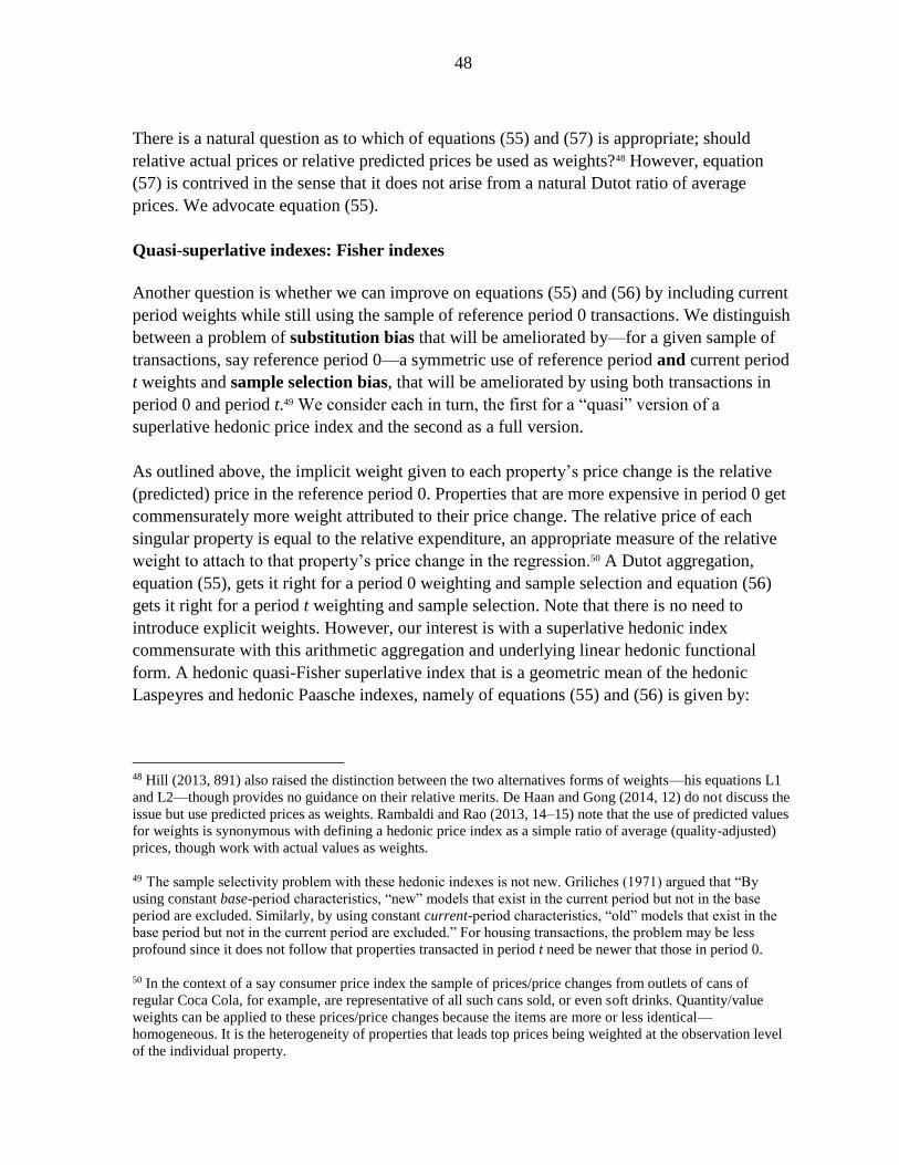
48
There is a natural question as to which of equations (55) and (57) is appropriate; should
relative actual prices or relative predicted prices be used as weights?48 However, equation
(57) is contrived in the sense that it does not arise from a natural Dutot ratio of average
prices. We advocate equation (55).
Quasi-superlative indexes: Fisher indexes
Another question is whether we can improve on equations (55) and (56) by including current
period weights while still using the sample of reference period 0 transactions. We distinguish
between a problem of substitution bias that will be ameliorated by—for a given sample of
transactions, say reference period 0—a symmetric use of reference period and current period
t weights and sample selection bias, that will be ameliorated by using both transactions in
period 0 and period t.49 We consider each in turn, the first for a “quasi” version of a
superlative hedonic price index and the second as a full version.
As outlined above, the implicit weight given to each property’s price change is the relative
(predicted) price in the reference period 0. Properties that are more expensive in period 0 get
commensurately more weight attributed to their price change. The relative price of each
singular property is equal to the relative expenditure, an appropriate measure of the relative
weight to attach to that property’s price change in the regression.50 A Dutot aggregation,
equation (55), gets it right for a period 0 weighting and sample selection and equation (56)
gets it right for a period t weighting and sample selection. Note that there is no need to
introduce explicit weights. However, our interest is with a superlative hedonic index
commensurate with this arithmetic aggregation and underlying linear hedonic functional
form. A hedonic quasi-Fisher superlative index that is a geometric mean of the hedonic
Laspeyres and hedonic Paasche indexes, namely of equations (55) and (56) is given by:
48 Hill (2013, 891) also raised the distinction between the two alternatives forms of weights—his equations L1
and L2—though provides no guidance on their relative merits. De Haan and Gong (2014, 12) do not discuss the
issue but use predicted prices as weights. Rambaldi and Rao (2013, 14–15) note that the use of predicted values
for weights is synonymous with defining a hedonic price index as a simple ratio of average (quality-adjusted)
prices, though work with actual values as weights.
49 The sample selectivity problem with these hedonic indexes is not new. Griliches (1971) argued that “By
using constant base-period characteristics, “new” models that exist in the current period but not in the base
period are excluded. Similarly, by using constant current-period characteristics, “old” models that exist in the
base period but not in the current period are excluded.” For housing transactions, the problem may be less
profound since it does not follow that properties transacted in period t need be newer that those in period 0.
50 In the context of a say consumer price index the sample of prices/price changes from outlets of cans of
regular Coca Cola, for example, are representative of all such cans sold, or even soft drinks. Quantity/value
weights can be applied to these prices/price changes because the items are more or less identical—
homogeneous. It is the heterogeneity of properties that leads top prices being weighted at the observation level
of the individual property.
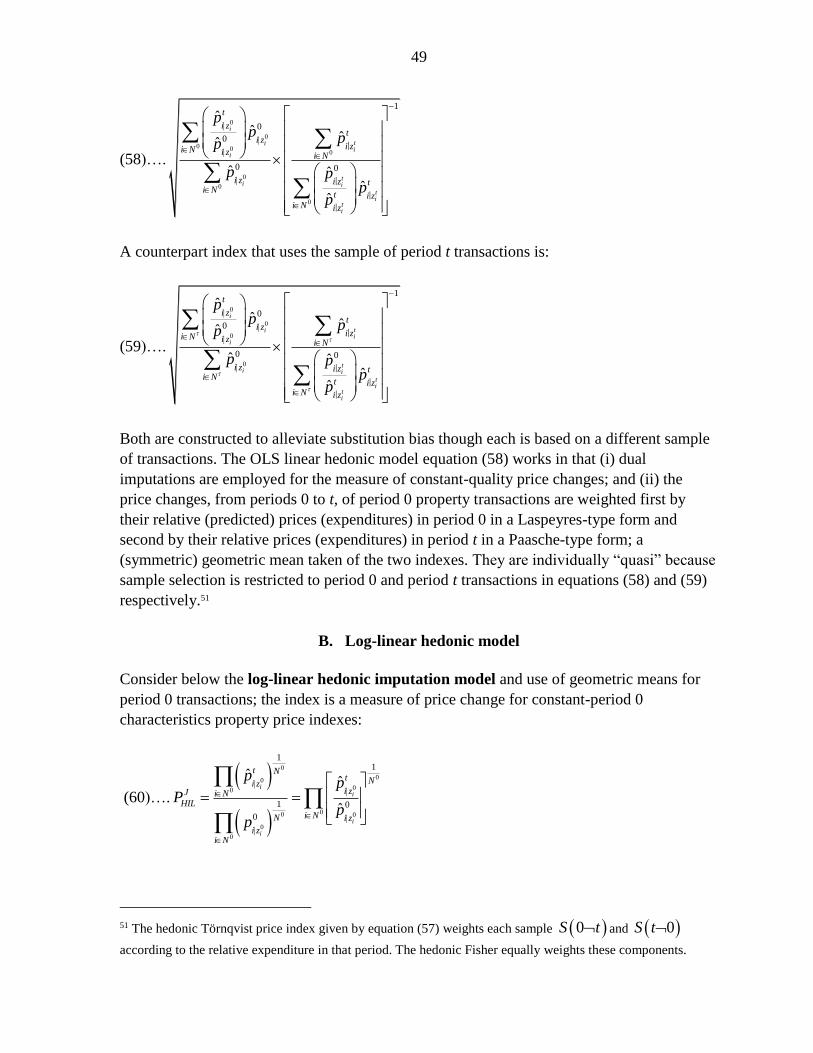
49
(58)….
0
0
0 00
0
0
0
1
0
0
0 0
ˆˆ ˆˆ
ˆ ˆˆ
ˆ
i
tii
i
ti i
ti
ti
t
i zt
i zi zi N i z i N
i z i z ti N
t i zi N i z
pp pp
p pp
p
|
|
|
|
A counterpart index that uses the sample of period t transactions is:
(59)….
0
0
0
0
1
0
0
0 0
ˆˆ ˆˆ
ˆ ˆˆ
ˆ
i
tii
i
ti i
ti
ti
t
i zt
i zi zi N i z i N
i z i z ti N
t i zi N i z
pp pp
p pp
p
|
|
|
|
Both are constructed to alleviate substitution bias though each is based on a different sample
of transactions. The OLS linear hedonic model equation (58) works in that (i) dual
imputations are employed for the measure of constant-quality price changes; and (ii) the
price changes, from periods 0 to t, of period 0 property transactions are weighted first by
their relative (predicted) prices (expenditures) in period 0 in a Laspeyres-type form and
second by their relative prices (expenditures) in period t in a Paasche-type form; a
(symmetric) geometric mean taken of the two indexes. They are individually “quasi” because
sample selection is restricted to period 0 and period t transactions in equations (58) and (59)
respectively.51
B. Log-linear hedonic model
Consider below the log-linear hedonic imputation model and use of geometric means for
period 0 transactions; the index is a measure of price change for constant-period 0
characteristics property price indexes:
(60)….
0
00
00
00 0
0
0
11
1 0
0
ˆˆ
ˆ
ii
i
i
t Nt Ni zi zJ i N
HIL
i NN i z
i zi N
pp
Pp
p
51 The hedonic Törnqvist price index given by equation (57) weights each sample 0S t and 0S t
according to the relative expenditure in that period. The hedonic Fisher equally weights these components.
50
Unlike the linear arithmetic case above, equal weights are implicitly attached to each price
change—such indexes are generally referred to as “unweighted” indexes. The price change
measured here is based on predicted values for reasons similar to those given above for the
arithmetic aggregation. There are three problems with this measure: (i) property price
changes are equally weighted; (ii) the index is based on only the sample of properties
transacted in period 0; and (iii) the introduction of explicit weights precludes our previous
use of equating average predicted prices to average actual prices, as a means by which dual
imputations are introduced. We consider each in turn.
Application of explicit reference and current period weights: a hedonic quasi-Törnqvist
price index
The first task is to apply weights to these price changes. A useful opportunity exists using the
imputation approach to explicitly introduce weights at this very lowest level. The approach,
to the author’s knowledge, was first proposed in Feenstra (1995) and used by Ioannidis and
Silver (1999) in an application, using scanner data, of hedonic methods to the quality
adjustment price indexes for television sets, but has not since received attention.
As outlined in section IIB, the imputation approach works at the level of individual
properties, rather than the average values of their characteristics. This allows us to explicitly
attach to each property’s price change a weight. Period 0 weights would be 0
0
0
0
0
ˆ
ˆi
i
i z
i zi N
p
p
given to
each price change, 0
0
0
ˆ
ˆi
i
t
i z
i z
p
p
in equation (55). We explicitly weight price changes by their
relative (predicted) price/transaction value in period 0. The price changes of more expensive
properties are given a higher (period 0) proportionate weight:
(61)….
00
00
0 0 00
0
00 0 0 0
0
ˆ
0ˆ
0,
0 0 0:
ˆ ˆ ˆexp ln
ˆ ˆ ˆ
i zi
i zii i ii N
i
i i i
p
t tpi z i z i zt
HGL zi Ni N i z i z i z
i N
p p pP
p p p
There is then the question of why only period 0 weights are used for this measure of constant
quality price change. We can use a symmetric average of period 0 and period t weights: a
hedonic quasi-Törnqvist price index but based on a period 0 sample selections given by:
51
(62)….
0
0 00
0
ˆˆ
0, 0
0 0: ˆ0
ˆ ˆ ˆexp ln exp lnˆ ˆ
ˆ
i
itit t
i i
t t ti i ii
t ti it
i
wtw
t ti z
i z i zt ti Ni iHGP z i z i zw
i N i Ni N i z i zi z
i N
pp p
P w w p pp p
p
where
0 0
0
0
ˆ ˆ1ˆ
ˆ ˆ2
t ti i
t ti i
t
i z i z
i t
i z i zi N i N
p pw
p p
which is a quasi-hedonic formulation of a Törnqvist index
(Feenstra, 1995, Ioannidis and Silver, 1999, and Balk, 2008), an index that has excellent
properties in economic theory as a superlative index (Diewert, 2004). It is “quasi” in the
sense that it does not make use of period t transactions.
Equation (62) uses a period 0 sample of transactions. A similar quasi-hedonic Törnqvist
index based on period t transactions is given by:
(63)…. ˆ
0
0 0ˆ ˆ ˆexp ln exp ln
ˆ ˆ
i
t ti i
t ti it tt t t
i i
wt t
i z i zJ t
HIGP i i i z i zi N i Ni N i z i z
p pP w w p p
p p
These innovative quasi hedonic superlative formulas depart from conventional hedonic
formulations—Diewert (2003), de Haan (2004a), Silver and Heravi (2005), de Haan and
Krsinich (2014, Appendix A) —in which the weights attached to each price change for
transactions in period 0 are the relative expenditures in period 0 (for 0i N ) and for period t
are the relative expenditures in t, (for ti N ), as opposed to an average of period 0 and t, as
in equations (52) and (53). Given, say, using equation (50) for period 0 transactions, we have
a comparison between actual prices in period 0 and counterfactual predicted prices in period
t, and given that these predicted prices act as corresponding weights in period t for the price
change, it would be wasteful to abandon the thought experiment for the weights but not for
the price change. Indeed abandoning ˆiw in favor of 0ˆiw would remove the analytical power of
taking some account of substitution bias.
C. The nature of substitution bias for a hedonic price index
A concern with both (geometric) Laspeyres-and Paasche-indexes is that they are both subject
to substitution bias. They form bounds on a superlative index, an index that has good
approximation properties to a theoretical index that does not have any substitution bias. A
periodically updated or chained Laspeyres or Paasche may alleviate substitution bias and be
closer to a theoretical index than its fixed base counterpart (Balk, 2008: 122–126).
52
Consider each property to have, for the large part, a unique seller and is open for purchase to
many buyers. Buyers can respond to above average characteristic price increases, say of extra
square footage and below average price increases of an additional bedroom by favoring
larger properties with fewer bedrooms, though with a delay to the purchase in thin markets.
A Paasche-type hedonic price index holds quantities of characteristics constant in the current
period and has a substitution bias in that their current period weight over-emphasizes the
substitution of purchases to properties whose characteristics have above average price
increases. Laspeyres-type characteristic price indexes understate a true Laspeyres-type index
and Paasche-type characteristic price indexes overstate a true Paasche-type characteristics’
price index.
The bounds can also be considered from a producer’s perspective. Assume a builder of an
apartment block has the flexibility to reconfigure some of the tied characteristics of the
apartments when near completion; again say an additional bedroom can be substituted for a
smaller area space of the living room, master bedroom and bathroom. If the characteristic
price of an additional bedroom increased faster than that of the concomitant increased
“living” square footage, a revenue-maximizing producer would substitute bedrooms for
living space. The supply side has a substitution towards property characteristics with above
average price increases and Paasche-type index would understate a true Paasche-type
hedonic index. Retrospective Paasche-type and quasi-Fisher hedonic price indexes can be
calculated and the empirical placing of the bounds, whether upper or lower, can be
determined and considered alongside a priori reasoning. As a result, a Paasche-type property
price index derived from equation (35) can be properly interpreted in terms of substitution
bias.
D. Hedonic superlative indexes and sample selection bias
The quasi-hedonic Fisher indexes in equations (58) and (59) were each based on samples of
period 0 and t transactions respectively as were the quasi-Törnqvist indexes in equations (63)
and (64). In both cases the problem is not one of substitution bias; it is a sample selection
bias. Substitution bias arises from using, in this context, period 0 or period t weights, rather
than a symmetric mean of the two period’s expenditure weights, as in a Törnqvist (or of
quantities, as in a Walsh) price index number formulas, or a symmetric mean of formulas that
respectively utilize period 0 and period t weights, as in a Fisher price index. The quasi-
superlative formulas outlined above make symmetric use of both periods’ weights, but limits
the sample to transactions either period 0 or period t. Our hedonic Fisher and our hedonic
Törnqvist price index should be based on samples of period 0 and period t transactions.
Some additional notation may help clarify the formulas. Let 0S t be the set of
properties that are present in both periods 0 and t, 0S t is the set of properties that are
present in period 0 but not period t, 0S t is the set of properties that are present in period
53
t but not period 0, and 0S t the set properties transacted in both periods. The weights
for each term are the relative transaction values of these sets of data. The weights for each
term are the relative transaction values of these sets of data, that is, where V is the total
value of transaction prices (or stocks) for 0S t , 0S t and 0S t ,
( 0) (0 ) (0 ) ii S t S t S tV v
;
0 0t ii tv v
,0 0t ii t
v v ; and
0 0t ii tv v
and iw is
an arithmetic mean of the weight (relative stock value or transaction (price) value) given to
each property in periods 0 and t, that is 01ˆ ˆ ˆ
2
t
i i iw w w . Bear in mind that we are
weighting the price change of each individual property and the weight is the relative
expenditure which equates to the price of the property. In this unusual situation we can use
predicted prices for weights, as argued above:
0
0
0
0 0
ˆ ˆ1 1ˆ ˆ ˆ
ˆ ˆ2 2
t ti i
t ti i
t
i z i z t
i i it
i z i zi S t i S t
p pw w w
p p
. The hedonic Törnqvist price index is:
(64)....
0 00
, ,
ˆ ˆˆ
0,
0 0 0:0 0 0
ˆ ˆ ˆ
ˆ ˆ ˆ
t tti ii
t t ti i i
ti
t t ti i k i k
v vvw ww
t t tV VV
i z i z i zt
HGP zi S t i S t i S ti z i z i z
p p pP
p p p
The superlative Törnqvist hedonic price index follows Triplett and McDonald (1977),
Diewert (2002), Triplett (2006), de Haan (2004a), and Silver and Heravi (2005).52 We note
that for repeat sales, (0 )S t , we have used a double imputation, that is predicted prices,
when actual prices are available. At first sight this goes against the principles of matched
models measurement whereby actual prices are compared, say for the price change of a
single standard can of Coca Cola for a consumer price index: the price of like is compared
over time with the price of like. However, as Hill and Melser (2008) explain:
“As far as we are aware, the possibility of always imputing for a repeat observation
….. has not previously been considered in the literature. For the case of computers,
this would be hard to justify since a particular model is the same irrespective of when
it is sold. Housing, however, is another matter. There is no guarantee even for a
repeat sale that we are comparing like with like. This is because the characteristics of
a house may change over time due to renovations or the building of a new shopping
center nearby, etc. The only way to be sure that like is compared with like is to
double impute all houses (even with repeat sales).” Hill and Melser (2008, page 600).
52 This paper acknowledges the contribution from Erwin Diewert (University of British Columbia) who
helpfully provided rigorous derivations of the results in a previous working version of this paper.
54
Equation (66) has the following attributes:
Its general form is a Törnqvist index, a superlative price index—an index number
formulas with good approximation to a price index without substitution bias. 53
It has no sample selectivity bias in that it includes estimates of constant quality price
change using three sets of price observations: (i) transacted in period 0 (but not in
period t); (ii) price observations transacted in period t (not in period 0); and (iii) repeat
price transactions available in both periods 0 and t.
For the aggregate of each set of transactions is weighted by the expenditure share of
that set, for example, if there are few repeat transactions in periods 0 and t, these price
changes have a commensurately less weight, 0 tv V . This is appropriate for a sample
selection issue.
For each of these sets of price observations, weights are estimated for both the reference
and current periods and a symmetric average of these two weights used,
0ˆ ˆ ˆ / 2ti i iw w w , akin to a superlative Törnqvist formulation.
A dual imputation is used for the constant quality price change and, for the weights,
relative predicted values for reasons outlined below.
E. Hedonic superlative price index number formulas: Hill and Melser (2008)
Our formulation of a hedonic superlative index, equation (59), differs from Hill and Melser
(2008)—hereafter HM—reiterated in Hill (2013) and used by Rambaldi and Rao (2013).54
Hill and Melser (2008, pages 601–602) derive hedonic Fisher and Törnqvist hedonic price
indexes from the imputation and characteristics approach for a semi-logarithmic functional
form of a hedonic regression. In an important contribution they first, show how the
derivations from the two approaches provide the same results. Second, they solve the absence
of matched models (infrequent transactions) by separately considering a geometric Laspeyres
for (constant
period 0 characteristics) and a geometric Paasche indexes (for constant period t
characteristic), and then taking a geometric mean of the two to derive a superlative hedonic
price index. We show both of these below but take issue with their formulation of a hedonic
superlative price index compared with our equation (64).
Hill and Melser (2008, page 601) show how a geometric Laspeyres hedonic price index
from an imputation approach equates to one from a characteristics approach:
53 For matched models of actual transaction prices, the Törnqvist index is given by
,0 ,
0
1
/2
,
,0
i i tN
t
T
i
s s
i t
i
pI
p
.
54 De Haan and Diewert (2013) in the RPPI Handbook (Eurostat et. al., 2013) have a similar formulation to Hill
and Melser (2008) except that it is unweighted.
55
(65)....
00
0
00
0 00
0 0 00 0
0 0 0
,0 00
ˆ ˆˆ ˆexp
ˆ ˆ
i zii
i zii ii N
i i
p
wt tp Ki z i z t
i k k i c
ki N i N i Ni z i z
p pw z
p p
0
0 0 0 0 0
, ,
0 0
ˆ ˆ ˆ ˆexp expK K
t t
k k i i c k k i c
k ki N
w z z
where 0 0
0
0 0 0
i ii i z i z
i N
w p p
and 0
0 0 0
,k i i k
i k N
z w z
is an arithmetic mean and the 0ˆi
t
i zp
and 0
0ˆii z
p
are generated from semi-logarithmic hedonic regressions.
The derivation is helpful since it clearly shows how weights are introduced into a
characteristics approach via the measure of the average value of each k characteristic,
0
0 0 0
,k i i k
i k N
z w z
. Compilers simply have to take their explicit weights, the relative price
0 0
0
0 0 0
i ii i z i z
i N
w p p
, for each transaction, and multiply them by the corresponding
characteristics values. This is equivalent to the hedonic imputation approach which we
focus on here as a more natural formulation in this context for dealing with aggregating over
predicted values of each property transacted with associated weights.55
The geometric Paasche version of equation (65) is:
(66).... 0
,00
ˆˆ ˆexp
ˆ
ti
ti
t ti
wt
Ki z t t
k k i c
ki N i z
pz
p
and a superlative formulation covering 0 ti N N is a geometric mean of the period 0 and
period t hedonic indexes:
(67)....
0
0
0
0 0
0 000 0
ˆ ˆ 1 ˆ ˆexpˆ ˆ 2
ti i
ti i
tii
w wt t
Ki z i z t t
i ik kki S t S t i zi z
p pz z
p p
.
55 Using an arithmetic formulation for the Dutot period 0 hedonic imputation-to-characteristics approach:
0
0
0
0 00
0
00 0
0 0 0 0 0 0
, ,0 0 00 0 0
00 0 0 00 0
, ,
0 00
1
1
ˆ ˆ ˆˆ ˆ ˆ
ˆ ˆ ˆ
ˆ ˆˆ
i
i
t t tK K Kt k k k
k k i k k i k ki zk k ki N i Ni N k k k
K KK
i zk k i k kk k i
i Nk kki N i N
N
N
z z zp
pz zz
where
0
kz is a weighted mean.
56
Note that this formulation differs from the one we proposed in equation (64) in some
important respects:
While the HM formulation captures the samples of transactions in periods 0 and t, it
does not include the symmetric weights of each transaction, as does the quasi-
Törnqvist hedonic indexes of equations (67) and (68) and superlative hedonic
formulation of equation (72). The HM formulation cannot take account of
substitution effects since the price change of a property is not weighted by a
(symmetric or otherwise) average of reference and current period weights. Price
changes of period 0 transactions are weighted by 0iw and price changes of period t
transactions by tiw , as opposed to ˆiw .
We advocate the use of the predicted values of prices as expenditure weights rather
than HM’s use of actual values.56 In the HM formulation period 0 observations are
weighted only by (actual) period 0 prices. Period t weights are not used to weight
these observations since HM only uses actual prices and there are no actual prices
for the counterfactual price of period 0 characteristics at period t prices. In our
formulation each period 0 observation’s price change and each period t
observation’s price change has an average of their corresponding period 0 and
period t (predicted) weights. Thus we include an approximation of substitution
effects for constant quality price change of period 0 transactions, and similarly for
price change observations in period t.
The sets of the price changes in the HM approach, 0S t and 0S t , are not
weighted according to their sample sizes. A symmetric mean is taken akin to a
superlative index. But this is to confuse the use of symmetric mean when
considering the weights of a price change, with a sample selection issue.
The functional form is complicated by the use of actual values for weights. A simple
ratio of arithmetic mean average prices between periods t and 0 for a constant period
0 characteristic hedonic price index from a linear hedonic regression is given by:
(68)....0
0
0 0 0
0 0 00
0 0 00 0 00
0 0
0 0 00
0 0 0
0 0 0
0
0 0 00
1
1
ˆ ˆ ˆˆ ˆˆ ˆ ˆ ˆ
ˆ
i i i
i i ii
i i i
i i
t t t
i z i z i zt
i z i z i zi z i N i N i Ni z i z i zt i N
HID
ii z i zi
i N i N i Ni N
N
N
p p pp p pp p p p
Pp p p
p
56 The difference arises because Hill and Melser (2008, page 600) argue for the use of predicted values (double
imputation) for the price change measurement but against the use of predicted values for weights due to a
possible mis-measurement error for these predicted price levels. However, first the weights are relative values,
not levels, and thus less prone to such error. Second, the omission of current period 0 (period t) weights for
period t (period 0) observations which requires predicted values (prices) could be more problematic.
57
a straightforward representation as a price (expenditure) weighted average of
constant quality price changes (dual imputation) if predicted values are used as
weights.
HM’s formulation omits a separate term 0S t but this is on the basis that there
are usually relatively few such observations, though exceptions may exist such as for
Tokyo apartments, Shimizu et al. (2010).
F. Weights for the time dummy approach
The time dummy hedonic price change estimates based on equations (8) (a linear functional
form) and (9) (a log-linear functional form) are estimates of ratios of arithmetic and
geometric mean prices respectively, controlling for (partial-out) changes in the quality mix.
Of note, for both linear and log-linear functional forms, is that the quality-mix adjustment
might have been valued at period 0 or at period t (=1) characteristic prices, but in this time
dummy formulation is constrained over the two periods to be identical, 0 1t
k k k .
The imputation approach, and by equivalence, the characteristics approach, have a major
advantage over the time approach since they can readily facilitate the introduction of explicit
weights at the level of the individual property. Unlike the hedonic imputation and
characteristics approaches, the time dummy estimate of constant quality price change comes
directly from the estimated coefficients of the regression itself. The introduction of explicit
weights has to be undertaken as part of the estimation.
Diewert (2002 and 2005) in seminal papers on weighted aggregation in regression argued for
a weighted least squares (WLS) estimator using expenditure shares as weights. He showed
that in a model for a bilateral two-period aggregate price comparison with average
expenditure shares ,0 , 2/i i tw w used as weights in a WLS estimator, the estimated price
change will be equivalent to the superlative Törnqvist index.57 Further contributions on
developing (value-share) weighting systems in regression-based estimates of aggregate price
change include Silver (2002), de Haan (2004), Diewert, Heravi and Silver (2009), de Haan
(2004 and 2009), Ivancic, Diewert, and Fox (2009), and de Haan and Krsinich (2014), and
for the cross country-product dummy approach, Diewert (2004 and 2005) and Rao (2005).
Leverage effects and the need for outlier detection and robust estimators
57 The Törnqvist index is given by
,0 ,
0
1
/2
,
,0
i i tN
t
T
i
s s
i t
i
pI
p
. See Diewert (1976 and 1978) for its superlative
properties.
(continued…)
58
Silver (2002)58 raised a concern with influential observations. First, as outlined in more detail
in Annex 2, there is the effect of an outlier on the estimated coefficients in a hedonic
regression. In a time dummy regression a, for example, property price observation whose
characteristics differ markedly from the mean of the transaction sample and whose price is
not well predicted by the regression—has relatively large residuals—can have a
weight/influence in determining the constant-quality price change that is markedly greater
than its singular transaction price deserves. Moreover, even if it had a larger explicit
expenditure weight attached to it using WLS, its overall influence would still be greater than
that merited by its expenditure weight.
Following Davidson and MacKinnon (1993), we first note that an OLS vector of β estimates
is a weighted average of the individual p elements, the prices of individual properties,
(69)…. ˆ -1
T Tβ X X X p
where the matrix X are the explanatory variable and -1
T TX X X p are the implicit weights
given to the prices. Equation (61) clearly shows that the β estimate is a weighted average of
prices, p. Consider also a WLS estimator where the explicit weights W are expenditure
shares:
(70)…. ˆ -1
T Tβ X WX X Wp .
It is apparent from (69) and (70) that outliers with unusual values of X will have a stronger
influence in determining β , than observations which are clustered in a group. In normal
index number formulae, the weights given to price changes are expenditure shares, while in
the hedonic framework in equation (1) the results from an expenditure share weighted
hedonic regression will also be determined by the residuals and relative values of the X
characteristics. An older property, for example, may have unusually poor quality
characteristics, and an unusually low price given such characteristics, the relatively high
residuals and leverage giving it undue influence in spite of the weights W in equation (70).
Influence statistics are a method of discovering influential observations, or outliers. Measures
of leverage and residuals are readily available in econometric software as are regression
estimators robust to undue leverage.59 They are concerned with the detection of how different
an observation is from the other observations in an equation’s sample, the difference that a
single observation makes to the regression results, and use of robust estimators as an
alternative to OLS.
58 Much of this is drawn from a 2002 unpublished mimeo by the author, Cardiff University. 59 EViews, for example, provides least squares diagnostics for outlier detection, described in “Leverage
Plots” on page 218, six diagnostic statistics/tests of the “Influence of an observation,” page 220, and in Chapter
30, page 387, “Robust least squares” details of three robust estimators one of which has as its focus outliers
with high leverage. (EViews 9 User’s Guide, Irvine CA: March 2015).
59
The presence and effect of influential observations is not fatal to the use of WLS. A proposal
would be to first examine all observations with high leverage, residuals, and influence and
correct/delete those found to be the result of mis-measurement or being out of the scope of
the study. However, since residuals are in turn based on a regression equation that may be
influenced by outliers, care is necessary in the identification of outliers and alternative
measures of influence and Belsley, Kuh, and Welsch (2005), Chatterjee and Hadi (1986), and
Davidson and MacKinnon (1993) are instructive in this regard. Second, there would remain a
problem with observations with relatively high weights and high influence values having to
be downgraded. However, observations with high leverage may be unusual only because of
shortfalls in the sampling of clusters in this characteristics space and the appropriate action is
to take, where feasible, a larger sample. Third, there may be a set of observations that have
very small weights and whose price changes are not dissimilar to other observations, but
have relatively unusually high leverage. The regression should be run with and without these
observations to validate their inappropriate influence and the observations deleted as
appropriate. Fourth, there is a case for using a heteroskedastic-consistent covariance matrix
estimator (HCCME). MacKinnon and White (1985) outline the HC2 estimator which
replaces the squared OLS residuals 2ˆi by a term that includes the leverage, and similarly the
HC4 estimator proposed by Cribari-Neto (2004).60 The ith residual is inflated more (less)
when ih is large (small) relative to the average of the ih , which is k n , see MacKinnon
(2013). Finally, there is a very different approach due to Silver and Graf (2014) considered in
the context of panel data for property price inflation. Included in the regression is a spatial
autoregressive (SAR) term that aside from removing potential omitted-variable bias enables
an innovative weighting system for the aggregate price change measure.
Yet WLS has a more conventional use in econometrics. A WLS estimator may be
appropriate when the errors from estimated models are heteroskedastic. WLS can give more
weight to observations with less conditional variance, thereby decreasing the sampling
variance of the OLS estimator. An observation from a distribution with less conditional
variance is considered to be more informative (in a predictive sense), than an observation
from a distribution with a higher conditional variance. However, the use of WLS to introduce
weights related to expenditure shares may conflict with a possible use as a more appropriate
estimator when errors are heteroskedastic.
60 HC2 replaces the OLS residuals with
2
ˆ
1
i
ih
and HC4 with
2
ˆ
1i
i
ih
where, min(4, )
i inh k and n is the
number of observations and k the number of explanatory variables, ˆi the residuals. MacKinnon (2013 notes that
a few papers have taken different approaches. Furno (1996) uses residuals based on robust regression instead of
OLS residuals in order to minimize the impact of data points with high leverage. Qian and Wang (2001) and
Cribari-Neto and Lima (2010) explicitly correct the biases of various HCCMEs in the HCj series. The formulae
that result are considered to generally appear to be complicated and perhaps expensive to program when n is
large.
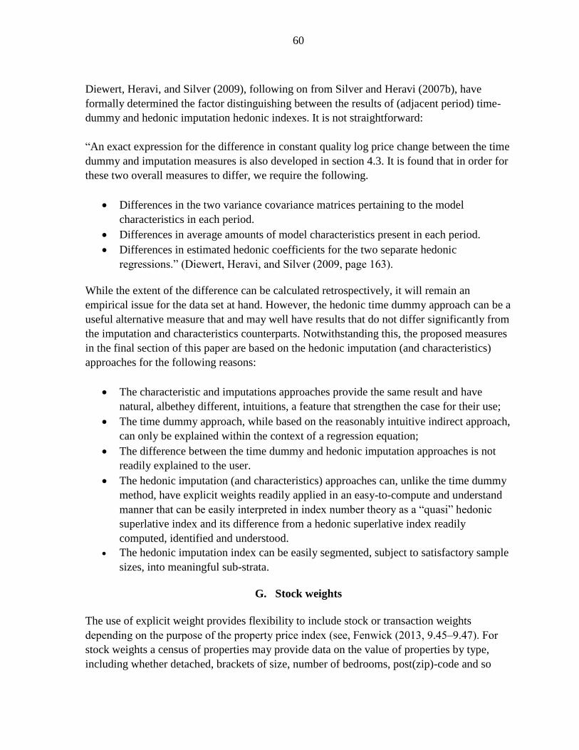
60
Diewert, Heravi, and Silver (2009), following on from Silver and Heravi (2007b), have
formally determined the factor distinguishing between the results of (adjacent period) time-
dummy and hedonic imputation hedonic indexes. It is not straightforward:
“An exact expression for the difference in constant quality log price change between the time
dummy and imputation measures is also developed in section 4.3. It is found that in order for
these two overall measures to differ, we require the following.
Differences in the two variance covariance matrices pertaining to the model
characteristics in each period.
Differences in average amounts of model characteristics present in each period.
Differences in estimated hedonic coefficients for the two separate hedonic
regressions.” (Diewert, Heravi, and Silver (2009, page 163).
While the extent of the difference can be calculated retrospectively, it will remain an
empirical issue for the data set at hand. However, the hedonic time dummy approach can be a
useful alternative measure that and may well have results that do not differ significantly from
the imputation and characteristics counterparts. Notwithstanding this, the proposed measures
in the final section of this paper are based on the hedonic imputation (and characteristics)
approaches for the following reasons:
The characteristic and imputations approaches provide the same result and have
natural, albethey different, intuitions, a feature that strengthen the case for their use;
The time dummy approach, while based on the reasonably intuitive indirect approach,
can only be explained within the context of a regression equation;
The difference between the time dummy and hedonic imputation approaches is not
readily explained to the user.
The hedonic imputation (and characteristics) approaches can, unlike the time dummy
method, have explicit weights readily applied in an easy-to-compute and understand
manner that can be easily interpreted in index number theory as a “quasi” hedonic
superlative index and its difference from a hedonic superlative index readily
computed, identified and understood.
The hedonic imputation index can be easily segmented, subject to satisfactory sample
sizes, into meaningful sub-strata.
G. Stock weights
The use of explicit weight provides flexibility to include stock or transaction weights
depending on the purpose of the property price index (see, Fenwick (2013, 9.45‒9.47). For
stock weights a census of properties may provide data on the value of properties by type,
including whether detached, brackets of size, number of bedrooms, post(zip)-code and so
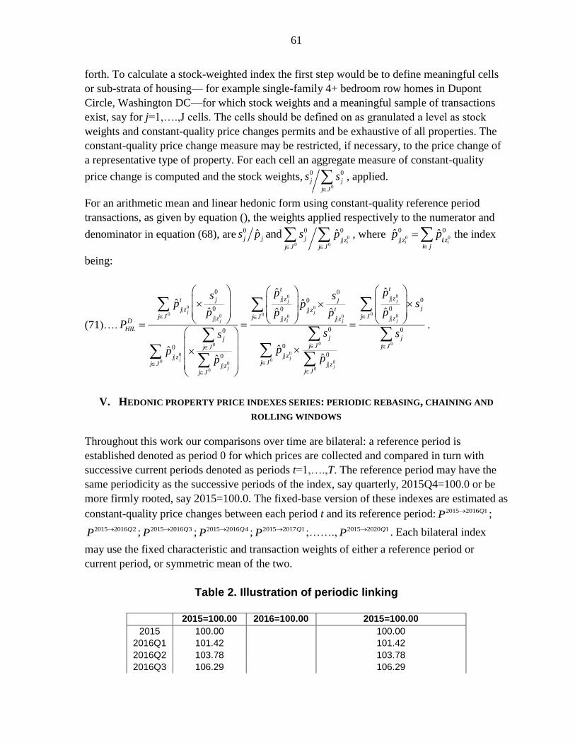
61
forth. To calculate a stock-weighted index the first step would be to define meaningful cells
or sub-strata of housing— for example single-family 4+ bedroom row homes in Dupont
Circle, Washington DC—for which stock weights and a meaningful sample of transactions
exist, say for j=1,….,J cells. The cells should be defined on as granulated a level as stock
weights and constant-quality price changes permits and be exhaustive of all properties. The
constant-quality price change measure may be restricted, if necessary, to the price change of
a representative type of property. For each cell an aggregate measure of constant-quality
price change is computed and the stock weights,0
0 0
j j
j J
s s
, applied.
For an arithmetic mean and linear hedonic form using constant-quality reference period
transactions, as given by equation (), the weights applied respectively to the numerator and
denominator in equation (68), are 0
0 0
0 0 0ˆ ˆandi
j j j j zj J j J
s p s p
, where 0 0
0 0ˆ ˆi ij z i z
i j
p p
the index
being:
(71)….
00
0 0
0 00 00 0
00
00
00 00
00
0 0
00
0 00
00
0000
ˆˆˆ ˆ
ˆ ˆˆ ˆ
ˆˆˆˆ
jj
j j
j ji j
jj
jj
tt
j zj zjt j
jtj z j zj J jj Jj z j zj z j zD
HIL
jjj Jj J
j zj zj Jj J j zj z
j Jj J
pps sp sp
p pp pP
ss
pppp
0
0
0
J
j
j J
s
.
V. HEDONIC PROPERTY PRICE INDEXES SERIES: PERIODIC REBASING, CHAINING AND
ROLLING WINDOWS
Throughout this work our comparisons over time are bilateral: a reference period is
established denoted as period 0 for which prices are collected and compared in turn with
successive current periods denoted as periods t=1,….,T. The reference period may have the
same periodicity as the successive periods of the index, say quarterly, 2015Q4=100.0 or be
more firmly rooted, say 2015=100.0. The fixed-base version of these indexes are estimated as
constant-quality price changes between each period t and its reference period: 2015 2016 1QP ;
2015 2016 2QP ; 2015 2016 3QP ; 2015 2016 4QP ; 2015 2017 1QP ;……., 2015 2020 1QP . Each bilateral index
may use the fixed characteristic and transaction weights of either a reference period or
current period, or symmetric mean of the two.
Table 2. Illustration of periodic linking
2015=100.00 2016=100.00 2015=100.00
2015 100.00 100.00
2016Q1 101.42 101.42
2016Q2 103.78 103.78
2016Q3 106.29 106.29
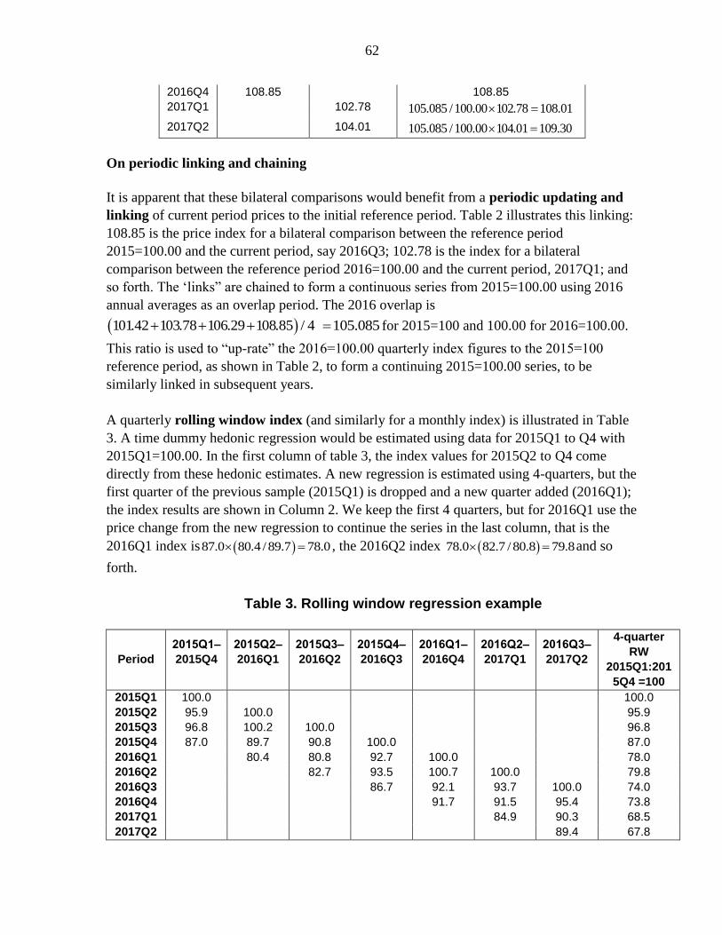
62
2016Q4 108.85 108.85
2017Q1 102.78 105.085 /100.00 102.78 108.01
2017Q2 104.01 105.085 /100.00 104.01 109.30
On periodic linking and chaining
It is apparent that these bilateral comparisons would benefit from a periodic updating and
linking of current period prices to the initial reference period. Table 2 illustrates this linking:
108.85 is the price index for a bilateral comparison between the reference period
2015=100.00 and the current period, say 2016Q3; 102.78 is the index for a bilateral
comparison between the reference period 2016=100.00 and the current period, 2017Q1; and
so forth. The ‘links” are chained to form a continuous series from 2015=100.00 using 2016
annual averages as an overlap period. The 2016 overlap is
101.42 103.78 106.29 108.85 / 4 105.085 for 2015=100 and 100.00 for 2016=100.00.
This ratio is used to “up-rate” the 2016=100.00 quarterly index figures to the 2015=100
reference period, as shown in Table 2, to form a continuing 2015=100.00 series, to be
similarly linked in subsequent years.
A quarterly rolling window index (and similarly for a monthly index) is illustrated in Table
3. A time dummy hedonic regression would be estimated using data for 2015Q1 to Q4 with
2015Q1=100.00. In the first column of table 3, the index values for 2015Q2 to Q4 come
directly from these hedonic estimates. A new regression is estimated using 4-quarters, but the
first quarter of the previous sample (2015Q1) is dropped and a new quarter added (2016Q1);
the index results are shown in Column 2. We keep the first 4 quarters, but for 2016Q1 use the
price change from the new regression to continue the series in the last column, that is the
2016Q1 index is 87.0 80.4 /89.7 78.0 , the 2016Q2 index 78.0 82.7 /80.8 79.8 and so
forth.
Table 3. Rolling window regression example
Period
2015Q1‒
2015Q4
2015Q2‒
2016Q1
2015Q3‒
2016Q2
2015Q4‒
2016Q3
2016Q1‒
2016Q4
2016Q2‒
2017Q1
2016Q3‒
2017Q2
4-quarter
RW
2015Q1:201
5Q4 =100
2015Q1 100.0 100.0
2015Q2 95.9 100.0 95.9
2015Q3 96.8 100.2 100.0 96.8
2015Q4 87.0 89.7 90.8 100.0 87.0
2016Q1 80.4 80.8 92.7 100.0 78.0
2016Q2 82.7 93.5 100.7 100.0 79.8
2016Q3 86.7 92.1 93.7 100.0 74.0
2016Q4 91.7 91.5 95.4 73.8
2017Q1 84.9 90.3 68.5
2017Q2 89.4 67.8
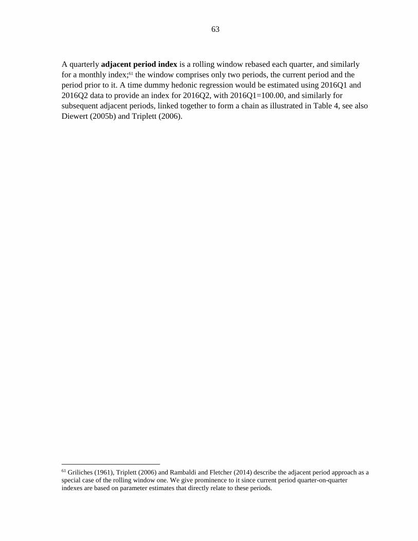
63
A quarterly adjacent period index is a rolling window rebased each quarter, and similarly
for a monthly index;61 the window comprises only two periods, the current period and the
period prior to it. A time dummy hedonic regression would be estimated using 2016Q1 and
2016Q2 data to provide an index for 2016Q2, with 2016Q1=100.00, and similarly for
subsequent adjacent periods, linked together to form a chain as illustrated in Table 4, see also
Diewert (2005b) and Triplett (2006).
61 Griliches (1961), Triplett (2006) and Rambaldi and Fletcher (2014) describe the adjacent period approach as a
special case of the rolling window one. We give prominence to it since current period quarter-on-quarter
indexes are based on parameter estimates that directly relate to these periods.
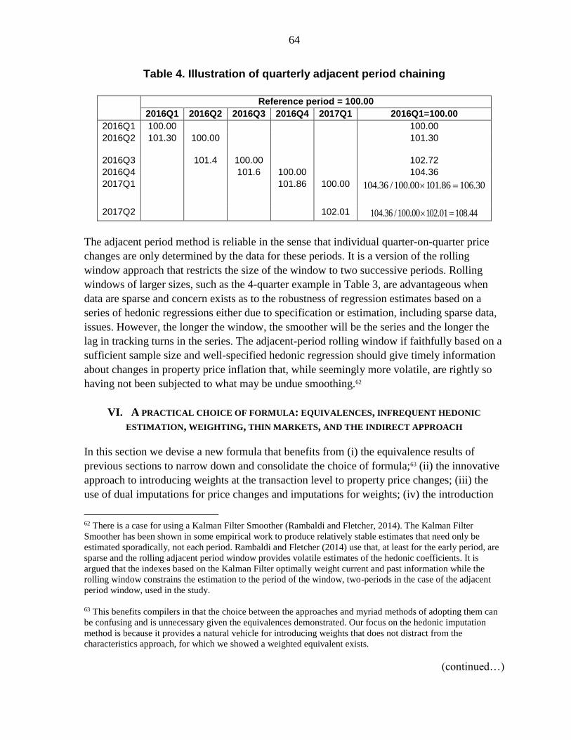
64
Table 4. Illustration of quarterly adjacent period chaining
Reference period = 100.00
2016Q1 2016Q2 2016Q3 2016Q4 2017Q1 2016Q1=100.00
2016Q1 100.00 100.00
2016Q2 101.30 100.00 101.30
2016Q3 101.4 100.00 102.72
2016Q4 101.6 100.00 104.36
2017Q1 101.86
100.00 104.36 /100.00 101.86 106.30
2017Q2 102.01 104.36 /100.00 102.01 108.44
The adjacent period method is reliable in the sense that individual quarter-on-quarter price
changes are only determined by the data for these periods. It is a version of the rolling
window approach that restricts the size of the window to two successive periods. Rolling
windows of larger sizes, such as the 4-quarter example in Table 3, are advantageous when
data are sparse and concern exists as to the robustness of regression estimates based on a
series of hedonic regressions either due to specification or estimation, including sparse data,
issues. However, the longer the window, the smoother will be the series and the longer the
lag in tracking turns in the series. The adjacent-period rolling window if faithfully based on a
sufficient sample size and well-specified hedonic regression should give timely information
about changes in property price inflation that, while seemingly more volatile, are rightly so
having not been subjected to what may be undue smoothing.62
VI. A PRACTICAL CHOICE OF FORMULA: EQUIVALENCES, INFREQUENT HEDONIC
ESTIMATION, WEIGHTING, THIN MARKETS, AND THE INDIRECT APPROACH
In this section we devise a new formula that benefits from (i) the equivalence results of
previous sections to narrow down and consolidate the choice of formula;63 (ii) the innovative
approach to introducing weights at the transaction level to property price changes; (iii) the
use of dual imputations for price changes and imputations for weights; (iv) the introduction
62 There is a case for using a Kalman Filter Smoother (Rambaldi and Fletcher, 2014). The Kalman Filter
Smoother has been shown in some empirical work to produce relatively stable estimates that need only be
estimated sporadically, not each period. Rambaldi and Fletcher (2014) use that, at least for the early period, are
sparse and the rolling adjacent period window provides volatile estimates of the hedonic coefficients. It is
argued that the indexes based on the Kalman Filter optimally weight current and past information while the
rolling window constrains the estimation to the period of the window, two-periods in the case of the adjacent
period window, used in the study.
63 This benefits compilers in that the choice between the approaches and myriad methods of adopting them can
be confusing and is unnecessary given the equivalences demonstrated. Our focus on the hedonic imputation
method is because it provides a natural vehicle for introducing weights that does not distract from the
characteristics approach, for which we showed a weighted equivalent exists.
(continued…)
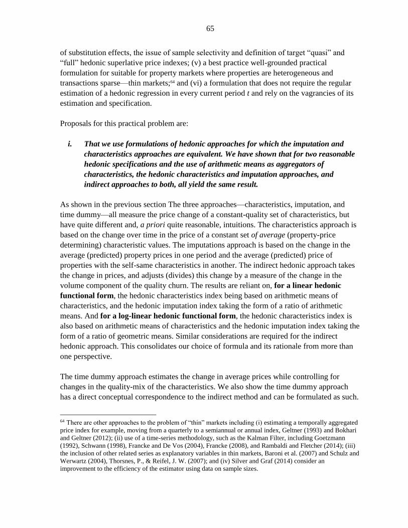
65
of substitution effects, the issue of sample selectivity and definition of target “quasi” and
“full” hedonic superlative price indexes; (v) a best practice well-grounded practical
formulation for suitable for property markets where properties are heterogeneous and
transactions sparse—thin markets;64 and (vi) a formulation that does not require the regular
estimation of a hedonic regression in every current period t and rely on the vagrancies of its
estimation and specification.
Proposals for this practical problem are:
i. That we use formulations of hedonic approaches for which the imputation and
characteristics approaches are equivalent. We have shown that for two reasonable
hedonic specifications and the use of arithmetic means as aggregators of
characteristics, the hedonic characteristics and imputation approaches, and
indirect approaches to both, all yield the same result.
As shown in the previous section The three approaches—characteristics, imputation, and
time dummy—all measure the price change of a constant-quality set of characteristics, but
have quite different and, a priori quite reasonable, intuitions. The characteristics approach is
based on the change over time in the price of a constant set of average (property-price
determining) characteristic values. The imputations approach is based on the change in the
average (predicted) property prices in one period and the average (predicted) price of
properties with the self-same characteristics in another. The indirect hedonic approach takes
the change in prices, and adjusts (divides) this change by a measure of the change in the
volume component of the quality churn. The results are reliant on, for a linear hedonic
functional form, the hedonic characteristics index being based on arithmetic means of
characteristics, and the hedonic imputation index taking the form of a ratio of arithmetic
means. And for a log-linear hedonic functional form, the hedonic characteristics index is
also based on arithmetic means of characteristics and the hedonic imputation index taking the
form of a ratio of geometric means. Similar considerations are required for the indirect
hedonic approach. This consolidates our choice of formula and its rationale from more than
one perspective.
The time dummy approach estimates the change in average prices while controlling for
changes in the quality-mix of the characteristics. We also show the time dummy approach
has a direct conceptual correspondence to the indirect method and can be formulated as such.
64 There are other approaches to the problem of “thin” markets including (i) estimating a temporally aggregated
price index for example, moving from a quarterly to a semiannual or annual index, Geltner (1993) and Bokhari
and Geltner (2012); (ii) use of a time-series methodology, such as the Kalman Filter, including Goetzmann
(1992), Schwann (1998), Francke and De Vos (2004), Francke (2008), and Rambaldi and Fletcher (2014); (iii)
the inclusion of other related series as explanatory variables in thin markets, Baroni et al. (2007) and Schulz and
Werwartz (2004), Thorsnes, P., & Reifel, J. W. (2007); and (iv) Silver and Graf (2014) consider an
improvement to the efficiency of the estimator using data on sample sizes.
66
These results concerning equivalences were outlined in detail in Section III. We thus
advocate the use of arithmetic means of characteristics as outlined in section II in the
compilation of both linear and log-linear hedonic approaches for the equivalences to
work.
ii. That a current period t formulation be used since the hedonic regression need only
be estimated for period 0
If a constant current period quality formulation is used for either of the approaches
considered above, the hedonic regression need only be estimated for period 0, that is:
Linear
(72a)….0 0
1 1
1 1
ˆ
ˆ ˆ
t t
t t
tit t
t ti it t
t t
i i zi N i N
i z i zi N i N
N N
N N
p p
p p
Log-linear
(72b)….
0 0
1 1
1 1
ˆexp ln exp
ˆ ˆexp ln exp
t t
t t
ti
t t
t ti it t
t t
i i zi N i N
i z i zi N i N
N N
N N
p p
p p
Note that actual values in the first term of equations (72a and b) are used in the numerators in
contrast to the imputed values of period t characteristics priced in period 0, in the
denominators. However, this is equivalent to a dual imputation because the average price
equals the predicted price in an OLS regression. The measure is of the price change of a
basket of constant current period t characteristics,t
iz , but only requires a hedonic regression
for period 0. Limiting the regression estimation to the reference period is a major advantage
given the critical role that hedonic estimates play in real estate property price. Having to only
estimate a hedonic regression for period 0 is a very attractive feature. Hedonic regression
estimates are subject to the vagrancies of specification and estimation procedures,
particularly in thin markets. A measure based on a well-grounded regression, especially one
based on an extended reference period as outlined in (ii) below, in turn better grounds the
index.
As explained in the previous section, the restricting of the sample of transactions to period t,
in a price comparison between periods 0 and t, is more concerned with than sample
selectivity bias than substitution bias. In the exploratory stage of calculating hedonic property
67
price indexes current and reference period formulations can be calculated and estimates of
sample selectivity bias derived and monitored.
iii. That an extended-current period formulation be used since sparse data is less
problematic
A major problem in RPPI and especially CPPI estimation is that of sparse data on
heterogeneous properties. However this can be alleviated by the use of an extended reference
period, noted as a useful feature of property price index construction by de Haan and Diewert
(2013).65 There may not be an adequate number of observations and/or variation in the
characteristics of the sample of properties transacted in period 0 to enable reliable and
pertinent estimates to be made of the coefficients of price-determining characteristics that
define properties sold in period t . For example, there may a relatively large, recently-built
retail property in a prime location (say postcode) sold in period t, but only a limited number
of retail properties sold in period 0 all of which are much smaller, older, and located in
poorer areas. The problem of sparse data prevents reliable estimates of the predicted price
from a period 0 regression of the period t characteristics.66 The current period formulation can
go some way to solving the problem of sparse data simply by defining the reference period 0,
for example, for a quarterly series 2016Q1, 2016Q2 etc., to be an extended period of say a
year with the index referenced as 2015=100.0 and centered at mid-2015. As such, the period
0 regression will be more likely to better encompass the characteristics of period t properties.
It is worth noting that the Paasche direct hedonic characteristics and imputation indexes and
the indirect counterparts all have this feature. The formulas using an extended reference
period are:
Linear
(73a)….
1 1
1 1
ˆ
ˆ ˆ
t t
t t
tit t
t ti it t
t t
i i zi N i N
er er
i z i zi N i N
N N
N N
p p
p p
65 Though de Haan and Diewert (2013) refer to it in the context of an advantage of the indirect method, similar
such formulations and advantages apply to the direct imputation and characteristics approach.
66 More formally, the width (standard error) of a prediction interval from a regression of ony x , for a given
value of say x x , depends not only on the fit of the regression—the larger the sample size and dispersion of
the explanatory variables, the smaller the interval— but also on the distance the given value of x is from the
sample mean x . The prediction will be better for values of x closer to x (Maddala and Lahiri, 2009).
68
Log linear
(73b)….
1 1
1 1
ˆexp ln exp
ˆ ˆexp ln exp
t t
t t
ti
t t
t ti it t
t t
i i zi N i N
er er
i z i zi N i N
N N
N N
p p
p p
iv. That the index be appropriately weighted at the lower level: weighting, quasi-
superlative indexes, and dual imputations
Arithmetic implicit weights and quasi-Fisher indexes
Weights are implicit in the functional form of the hedonic regressions and formula used to
average the prices. Given a linear functional form for the hedonic regression underlying the
(equivalent) characteristics and imputation approaches, the implicit weights given to each
property’s constant quality price change is the relative value of the property, a finding that
holds for the direct and indirect approaches. However, for the log-linear functional form of
the hedonic regression underlying the (equivalent) characteristics and imputation approaches,
equal weight is given to each constant-quality price change rather than the more desirable
transaction value. In section VI we outlined an approach to directly incorporating transaction
value weights into a hedonic imputation, and thus characteristics, approach for the log-linear
form. A linear/arithmetic index based on current period t transactions is defined as:
(74)….
1
0,
1:0 0
0
1 1ˆ ˆ
1 1 ˆˆ ˆˆ
ˆ
t ti it t t
ti
tt tii it t t
it ti
t t t
it t i z i zt i N i N i N
HDC z t
i ztt ti z i zi N i N i z
i N i z
p p pN N
Ppp p
pN Np
since for OLS: 0 0
0 0
0 0
0 01 1ˆ
i ii z i zi N i NN N
p p
.
A quasi-Fisher price index using period 0 and period t weights, but only price changes of
the period t sample of transactions, is given by:
(75)….
10
010
0
0 0
ˆ ˆˆ ˆˆ ˆ ˆ ˆ
ˆ ˆ ˆ ˆ
t ti i
t tt t i it tt ti it t i i
t t t ti i i it t t t
t
i z i z tt
ti z i zi z i z i N i Ni z i zi N i N
t t
i z i z i z i zi N i N i N i N
p pp pp p p p
p p p p
| |
| || |
| |
| | | |
.
69
Again, since for OLS: 0 0
0 0
0 0
0 01 1ˆ
i ii z i zi N i NN N
p p
; we do not need to estimate a hedonic
regression for period t .
Geometric explicit weights and quasi-Törnqvist indexes
For the log-linear formulation, a hedonic quasi-Törnqvist imputation index is:
(76)….
0
00
0
0
ˆˆ /2
ˆ/2 /2ˆ
0 0ˆ /20ˆ ˆˆ
t t
t t
t t
tt
i z i z ti i i ii it
ti z i z it ti i t
i ii N i N
ti it tt t
ti ii
t
p pw wt w w
t tp p i zi z i zJ i N
HIL w wi N i Ni z i z
i zi N
pp p
Pp pp
= 0 0ˆ ˆexp / 2 ln lnt ti it
t t
i i i z i zi N
w w p p
Now equation (76) differs from our Törnqvist imputation index in equation (59) in that
because we are not running period t hedonic regressions, there are no predicted period t
prices. Actual prices and weights are used for period t and dual imputation for the (logarithm
of the) price changes, are not possible. Workarounds are necessary to convert t
iw to ˆ t
iw and
ti
t
i zp
to ˆ ti
t
i zp
.67
v. That a workaround be applied to the log-linear case to (a) approximate predicted
values of prices and weights using actual values and (b) form dual imputations
An approximation for the predicted value of period t weights is:
(77)….
0 0
0 0
0 0
0 0
*
0 0
0 0
ˆ ˆ
ˆˆ ˆ
i i
i i t
t t
i z i zt t
i it o
i it i ii t o
i ii z i zt ti Ni i
i N i Ni i
p pp w
p p w ew
w ep pp w
p p
where o
ie is the error term from the
log-linear hedonic regression.
If the hedonic regression has a poor fit, especially for unusually high or low priced
properties, actual values could be used for weights in both periods: ** 0 / 2t
i i iw w w .
Retrospective studies using t
iw , *ˆ t
iw and **ˆ t
iw should be undertaken to compare the difference
in the results for the index.
67 An alternative is to use actual values as weights for both periods 0 and t as shown and discussed in section
IVA.
70
A workaround for the predicted value of period t prices for a dual imputation would be
to use the indirect method:
(78) has integrity in the sense that the ratio of average actual prices between periods 0 and t
in the numerator is of actual values, while the ratio in the denominator is a dual imputation,
of predicted prices. None of the terms require the estimation of a hedonic regression in period
t. It does not lead to our desired hedonic quasi-Törnqvist index of equation (5), but should be
a good approximation.
A reasonable stance is to accept equation (73) as is; the resulting index is an implied price
index born out of appropriate measures of the change in actual prices divided by the overall
change in characteristics volumes, the former comparing with actual prices and the latter
measured as a dual imputation. We denote this as option A.
However, option B is to develop a workaround for using predicted instead of actual period t
price. An alternative formulation of the indirect method is to use:
(74)….
0
0
00
00
0
00
0 00
0 0
00 0
exp ln
exp ln
ˆ ˆexp ln
exp ln
i
tt iti
t
i
ii
ti
t ti it t
i
w t tti i zi z
i Ni N
w
i i zi zi NJ i N
HIGL wt
ii z i zi N i N
w
ii i
i Ni N
w pp
w pp
P
p w p
p w p
0 0
exp ln
ˆexp ln
tit
tit
t t
i i zi N
i i zi N
w p
w p
Note that the bottom term in the denominator is now an actual, rather than predicted
transaction price. Again all terms can be calculated without estimating a hedonic regression
for period t. The advantage of the above formulation is that it cancels out to a ratio of two
terms, the meaningful price index, but that now the resulting index is a ratio of price changes,
the average actual price in period t of period t characteristics in the numerator and the
average predicted price in period 0 of period t characteristics in the denominator. The
disadvantage is that it is not a dual imputation.
71
To ameliorate any bias from the single imputation in equation (73) we, as a work-around,
apply a correction to ti
t
i zp|
to approximate ˆ ti
t
i zp|
. Instead of using 0 0
exp ln
ˆexp ln
t
tit
t t
i i
i N
i i zi N
w p
w p
from the
right hand side of equation (74), we use an estimate of the predicted value in the numerator:
(75)….0
0
*
0
ˆˆ ˆi
t ti i
i zt t t
ii z i zi
pp p p
p
|
| |.
The direct dual imputation from equation (74) is thus:
(76)….
0
0
*0
0 0 0 0
ˆexp ln ˆexp ln
ˆ ˆexp ln exp ln
i
ttit it
t ti i
t t
i zt tt t
i i z i i zi N ii N
i ii z i zi N i N
pw p w pp
w p w p
|
||
A concern is that *ˆ ti
t
i zp|
should have been estimated using the current period t ratio of actual to
predicted prices, rather than the period 0 ones in equation (74), that is:
(77) **ˆ
ˆ ˆti
t t ti i i
t
i zt t t
ti z i z i zi
pp p p
p
|
| | |.
However, this requires a hedonic regression estimated for period t. Some simple tests on
retrospective data should help with the choice between options A and B, and for option B,
using the (indirect) price index in equation (74) or the (direct) price index, with an
adjustment for double imputation, in equation (75).
Such tests may be based on estimating indexes from retrospective data for which period t can
hedonic regressions can be reliably estimated using ( *ˆ ti
t
i zp|
and **ˆ ti
t
i zp|
) in equations (75 and 78)
and comparing this with the results from using equation (59) that benefits from a period t
estimated hedonic regression. If the differences are relatively small over time, then the
adjustment may be used.68
68 We note here that a further development would be to use a mid-period valuation of the characteristics. At first
this has little meaning, because the characteristics do not change. The sample is of a set of transactions in period
t whose self-same characteristics are valued in period 0. However, if we apply period 0 weights to the
characteristic values and period t weights for period t average characteristic values, then a mid-period
(continued…)
72
vi. That an indirect approach be used
The indirect approach takes the change in prices, as in equation (78), and divides this by the
change in quality-mix, equation (79), to derive a measure of the change in constant quality
price change, equation (80), that is:
(78)….
0 0 0
0 0
0 0
1 1
1 1
ˆ
ˆ
t t tit t
i
t t
i i zi N i N
i i zi N i N
N N
N N
p p
p p
is the change in average (actual equal to predicted, for OLS)
prices; and
(79)….
0 0
0
0
1
1
ˆ
ˆ
t tit
it
i zi N
i zi N
N
N
p
p
is the change in the quality-characteristics value at constant period 0
prices.
Since 1
tt
t
i
i NNp
=1
ˆt
tit
t
i zi NN
p
for OLS, equation (79) divided by equation (78) equals:
(80)….0 0
0
0
0
00
0
1
1 1
11
1
ˆ
ˆ ˆ
ˆˆ
ˆ
t
t
tt
t
tit
ti it
ttii tt
it
t
i zi N
t
i z i zi N i N
i zi zi Ni N
i zi N
N
N N
NN
N
p
p p
pp
p
characteristic average value is meaningful. Advantages are outlined in Okamoto (2001). Diewert (2004, 15.49–
15.53), Hill (1998), and Hill (1990) and Baldwin (1990, 255–256), cited by Diewert (2004). Using the
characteristics approach based on average (weighted) mean characteristic values, a constant quality mid-period
characteristic value index can be devised and calculated. There would be the need for issues and workarounds to
be considered as to the use of imputations, but these could be resolved. Further details are from the author.
73
And for a log-linear form:
(81)…. 0
0
00 0
11
1 1
ˆˆ exp lnexp ln
ˆexp ln
ˆ ˆexp ln exp ln
tt
t t
ttii tt
ti it t
tt
i zi z Kt t i Ni N
k k k
k
i z i zi N i N
NN
N N
pp
z z
p p
is the constant (period t)-quality price index.
Since the indirect approach (equation (81)) provides the same result as the direct one, an
obvious question is: why we propose switching to the indirect one?
First, the indirect method is phrased to follow the intuition of the problem at hand. A change
in average prices is affected by a change in the quality mix of properties transacted each
period. Thus the need to identify price-determining characterizers and measure changes in
their average values, for example, on average, number of bedrooms, number of bathrooms,
square footage of lot, square footage of property, proportion in a specific postcode and so
forth. We take measures of changes in the average quantities of such characteristics to correct
for the change in the quality mix. The change in each characteristic’s average quantity is
valued (weighted) using the estimated valuations from a period 0 hedonic regression that
explains price variation in terms of its price-determining characteristics. A weak point of the
intuition for the direct approach, at least to the lay user, is that the essence of the measure is
the change in the marginal valuations of the characteristics from the estimated parameters of
hedonic regressions.
Second, the indirect formulation provides additional information: it takes the change in
average transactions prices, divides this by the explicitly-measured change in characteristic
mix via an identifiable measure of such changes. The constant-quality property price index
has an analytical decomposition as the change in price adjusted by the change in the quality-
mix of properties sold. The direction and extent of average price change, for example, going
into, during, and coming out of recessions can be analyzed in terms of the its constituent
product of quality mix and raw price change. Indeed, we can decompose the change in total
value of properties transacted to be the product of the change in the number of properties
transacted and changes in the average prices, and the change in average price to be the
product of the quality-adjusted and the change in the volume of quality:
(82)…. Value P Number .
and
(83)…. const qual qualityP P Volume .
74
vii. Segmentation and periodic updating of weights
The proposed formulas are for individual segments of properties, say terraced houses in a
major city. The index of price change for an individual segment can be aggregated with other
segments, say by location and then by type to form a national index. The weights might be
stock or transaction-value weights depending on purpose, Fenwick (2013). An advantage of
the hedonic imputation quasi-superlative formulation is that for each transaction in period t
there is a repeat valuation in period 0. Thus, sample sizes permitting, more granular results
within any segment can be given, depending on user needs.
The quasi-superlative formulation recommended here requires that only a reference period
hedonic regression be estimated. However, as with the rebasing of any price index number,
the estimated coefficients might soon become out of date. How “soon” is soon is an empirical
matter readily tested by estimating a pooled regression over a number of time periods, testing
for the constancy of the estimated coefficients over time and if failing, ascertaining the
magnitude of the change. Quarterly or monthly hedonic property price indexes might require
an updating of the reference period hedonic regression every two or three years, or possibly
annually.
75
VII. SUMMARY
For the hard problem of properly measuring RPPIs countries generally have available to
them only secondary data sources: from land registries/notaries, lenders, realtors, buyers, and
builders. Further, transactions of properties are infrequent and properties are heterogeneous.
Measures of average property price change can be confounded by changes in the quality-mix
of properties transacted between the two periods compared. Hedonic regressions have been
advocated as the primary method for adjusting measured price change for the change in the
quality-mix of transactions. De Haan and Diewert (2013) outline the three main approaches
to using hedonic regressions for this purpose, for which there are many forms, including
different forms of weights, sample selection, imputations, aggregators, direct and indirect
methods and no straightforward guidelines.
First, we demonstrate equivalencies between the approaches for quite straightforward
formulations of hedonic methods to narrow down the choice among formulas. We show that
the hedonic characteristics and imputations approaches give the same result as long as we
stick to a what are quite reasonable formulations of these methods. This is a major plus in
harmonizing and justifying hedonic methodologies.
Second, we devise an easily applicable and innovative form of weighting for these property
price indexes and, there from, derive quasi-superlative and superlative formulations of these
hedonic indexes that improve on those in the literature.
Third, arising from these derivations, we develop well-grounded practical measures of
hedonic property price inflation that are (i) suitable for thin markets and sparse data, (ii) not
subject to the vagrancies of the periodic estimation of hedonic regressions, (iii) benefit from
the innovative weighting system along with (iv) a “quasi” superlative formulation that should
take account of much of any substitution bias at this level (and does not require re-estimation
of the hedonic regression),69 and (v) has a justification on an intuitive level from both the
imputation and characteristics hedonic approaches, and (vi) can be readily segmented into
sub-aggregates.
69 The “quasi” superlative formulation is tightly phrased as a component of a hedonic superlative index and its
implicit assumptions are quite reasonable and easily testable using retrospective data.
76
ANNEX A. DIFFERENCE BETWEEN HEDONIC ARITHMETIC AND GEOMETRIC MEAN
PROPERTY PRICE INDEXES
Following Silver and Heravi (2007b), consider a sample Dutot index, DP , in equation (A1),
as a ratio of two sample arithmetic means of prices. The sample Dutot is a consistent, but not
unbiased, estimator of the ratio of population means, the population Dutot index,
(A1) ….00
E
E
t t
D
pI
p
.
The sample hedonic geometric Laspeyres-type index, JP , in equations (A2), is a ratio of the
exponents of two sample means of log prices and is a consistent estimator of the population
hedonic geometric Laspeyres-type index,
(A2)….
0
00
exp E log exp= exp
expexp E log
t t
t
J
pI
p
where
E logt tp and 0 0E log p
.
Since the exponential function cannot be taken through expected values:
(A6)…. E exp E log expp p for 0,t ,
and by Jensen’s inequality:
(A7)…. E exp E log expp p for 0,t .
As such the numerator of DI will exceed the numerator of JI , as will the denominator,
making it impossible to determine which effect will dominate, without making a further
distributional assumption.
We introduce the distributional assumption:
(A8)…. 2log ,p Normal
for 0,t .
It follows from the properties of a lognormal distribution that:
77
(A9)….. 2exp / 2
. for 0,t .
Substituting , for 0,t , in equation (A1) by equation (A6) and using equation (A2)
gives a relationship between the population Dutot and Hedonic geometric Laspeyres-type
indexes in terms of the difference in the variances of log-prices between periods 0 and t:
(A10)….
2 2
2 2
00 0 2 2
0 0
exp / 2 exp / 2.exp / 2
exp / 2 exp / 2
ttt t
D J J tI I I
.
It is apparent from equation (A10) that as product heterogeneity and price dispersion
decreases, so too will the difference between the two indexes. The above exposition carries
over to indexes that control for observable product heterogeneity through hedonic
regressions. Consider a regression, using data on m = 0,...,M matched models for periods
0,t , of the log of price, ln mp , on a dummy variable tD which takes the value of 0 in
period t and zero in a base period 0, and on k = 2,…,K quality characteristics, kmz :
(A11)…… 0 1
2
lnK
t
m k km m
k
p D z u
where mu is assumed to be normally distributed with mean and variance and 2
respectively. The hedonic (quality-adjusted) estimated geometric Laspeyres-type index is
given by:
(A12)…. *
1ˆexpJP
which, since matched models are used, is equal to the hedonic geometric Laspeyres-type
index in equation (A2). However, the Dutot index failed the commensurability test and is
thus itself determined by the extent of price dispersion. A consistent estimator of the hedonic
(quality-adjusted) Dutot index is given by:
(A13)…. * 2 2 * 2 2
1 0 0ˆˆ exp .exp / 2 .exp / 2D t J tI P
.
where the * denotes heterogeneity-adjusted and where 2
, for 0,t , are the variances of
the residuals of observations in periods 0 and t respectively. Thus the difference between the
hedonic geometric Laspeyres-type index and the Dutot hedonic price index is related to the
change in the variance of the residuals over time. If 2 2 2 2
0 0ˆ ˆt t (from (A11) and
(A7) respectively) then the discrepancy between the Dutot and hedonic geometric Laspeyres-
78
type indices in (00) will be greater than the discrepancy between the heterogeneity-controlled
Dutot and the hedonic geometric Laspeyres-type index in (A00). Note that first, for 0,t ,
as 2ˆ 0 , * *
D JP P . Second, 2 2 2 2
0 0ˆ ˆt t if the hedonic regression controls for the
same proportion of price variation in each period, that is 2 2ˆ for 0,t where
0 1t . Minimizing dispersion from product heterogeneity should account for some of
the difference between the Dutot and hedonic geometric Laspeyres-type indexes.
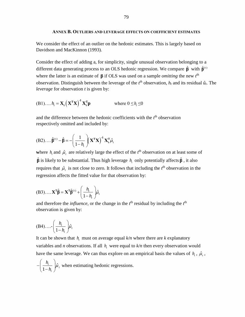
79
ANNEX B. OUTLIERS AND LEVERAGE EFFECTS ON COEFFICIENT ESTIMATES
We consider the effect of an outlier on the hedonic estimates. This is largely based on
Davidson and MacKinnon (1993).
Consider the effect of adding a, for simplicity, single unusual observation belonging to a
different data generating process to an OLS hedonic regression. We compare β with ( t )β
where the latter is an estimate of β if OLS was used on a sample omitting the new tth
observation. Distinguish between the leverage of the tth observation, ht and its residual ût. The
leverage for observation t is given by:
(B1)…. th -1
T T
t tX X X X p where 0 ≤ th ≤0
and the difference between the hedonic coefficients with the tth observation
respectively omitted and included by:
(B2)…. (t ) 1ˆ ˆ ˆ1
t
th
-1T T
tβ β X X X
where th and ˆt are relatively large the effect of the tth observation on at least some of
β is likely to be substantial. Thus high leverage th only potentially affects β , it also
requires that ˆt is not close to zero. It follows that including the tth observation in the
regression affects the fitted value for that observation by:
(B3)….(t )ˆ ˆ ˆ
1
tt
t
h
h
T TX β X β
and therefore the influence, or the change in the tth residual by including the tth
observation is given by:
(B4)….- ˆ1
tt
t
h
h
It can be shown that th must on average equal k/n where there are k explanatory
variables and n observations. If all th were equal to k/n then every observation would
have the same leverage. We can thus explore on an empirical basis the values of th , ˆt ,
ˆ1
tt
t
h
h
when estimating hedonic regressions.
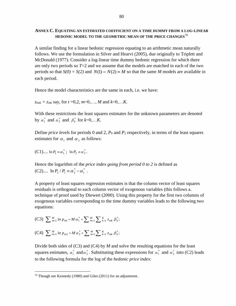
80
ANNEX C. EQUATING AN ESTIMATED COEFFICIENT ON A TIME DUMMY FROM A LOG-LINEAR
HEDONIC MODEL TO THE GEOMETRIC MEAN OF THE PRICE CHANGES70
A similar finding for a linear hedonic regression equating to an arithmetic mean naturally
follows. We use the formulation in Silver and Hearvi (2005), due originally to Triplett and
McDonald (1977). Consider a log-linear time dummy hedonic regression for which there
are only two periods so T=2 and we assume that the models are matched in each of the two
periods so that S(0) = S(2) and so that the same M models are available in
each period.
Hence the model characteristics are the same in each, i.e. we have:
zmtk = zmk say, for t =0,2, m=0,…, M and k=0,…K.
With these restrictions the least squares estimates for the unknown parameters are denoted
by and and for k=0,…K.
Define price levels for periods 0 and 2, P0 and P2 respectively, in terms of the least squares
estimates for 1 and
2 as follows:
(C1).... ; .
Hence the logarithm of the price index going from period 0 to 2 is defined as
(C2).... .
A property of least squares regression estimates is that the column vector of least squares
residuals is orthogonal to each column vector of exogenous variables (this follows a.
technique of proof used by Diewert (2000). Using this property for the first two columns of
exogenous variables corresponding to the time dummy variables leads to the following two
equations:
(C3)
(C4)
Divide both sides of (C3) and (C4) by M and solve the resulting equations for the least
squares estimates, and . Substituting these expressions for and into (C2) leads
to the following formula for the log of the hedonic price index:
70 Though see Kennedy (1980) and Giles (2011) for an adjustment.
MNN )2()1(
*1
*2 *
k
*11ln P *
22ln P
*
1
*
212 /ln PP
;1 *11
*111 kmk
Kk
Mmm
Mm zMpn
;1 *11
*221 kmk
Kk
Mmm
Mm zMpn
*1
*2 *
1*2
81
(C5) .
Taking exponents of both sides of (C5) shows that the hedonic model price index going
from period 0 to 2 under the above matched model conditions is equal to the equally
weighted geometric mean of the M model price relatives, which would be a conventional
matched model statistical agency estimate of the price index for this elementary group of
commodities.
121
*
1
*
212 /ln/1/ln mm
M
m ppMPP
82
References
Adelman, Irma and Zvi Griliches, 1961. On an index of quality change. Journal of the
American Statistical Association, 56, 295, 535-548.
Baldwin, Andrew 1990. Seasonal baskets in consumer price indexes, Journal of Official
Statistics, 6 ,3, September, 251–273.
Balk, Bert M. 1983. Does there exist a relation between inflation and relative price change
variability? The effect of the aggregation level, Economic. Letters 13, 2–3, 173–180.
Balk, Bert M. 2005. Price indexes for elementary aggregates: The sampling approach,
Journal of Official Statistics, 21, 4, 675-699.
Balk, Bert M. 2008. Price and Quantity Index Numbers, Cambridge: Cambridge University
Press.
Baroni, M., Barthélémy, F., & Mokrane, M. 2007. A PCA repeat sales index for apartment
prices in Paris, Journal of Real Estate Research 29, 137–158.
Belsley, David A., Edwin Kuh, and Roy E. Welsch 2005. Regression diagnostics: Identifying
influential data and sources of collinearity, vol. 571. John Wiley & Sons.
Berndt, Ernst R. 1991. The practice of econometrics: classic and contemporary Reading,
Massachusetts: Addison Wesley.
Berndt, Ernst R., and Zvi Griliches 1993. Price indexes for microcomputers: An exploratory
study. In Price measurement and their uses, ed. Murray F. Foss, Marilyn E. Manser,
and Allan H. Young, 63–93. Studies in Income and Wealth 57. Chicago: University
of Chicago Press.
Berndt, Ernst R., Zvi Griliches, and Neal. J. Rappaport. 1995. Econometric estimates of
different approaches to estimating hedonic price indexes for personal computers in
the 1990s. Journal of Econometric, 68, 1, 243–268.
Berndt, Ernst R., and Neal J. Rappaport 2001. Price and quality of desktop and mobile
personal computers: A quarter-century historical overview. American Economic
Review 91, 2, 268–273.
Bokhari, Sheharyar and David Geltner 2012. Estimating real estate price movement for high-
frequency tradable indexes in a scarce data environment, Journal of Real Estate
Finance and Economics, 45, 2, 522–543.
Case, Bradford, Henry O. Pollakowski and Susan M. Wachter, 1991 On Choosing Among
House Price Index Methodologies, Real Estate Economics, 19, 3, 286–307,
September.
Cassel, E. and Mendelsohn, R. 1985. The choice of functional forms for hedonic price
equations: comment. Journal of Urban Economics, 18, 2, 135-142.
83
Chatterjee, Samprit and Ali S. Hadi 1986. Influential observations, high leverage points, and
outliers in linear regression, Statistical Science, 1, 3, August, 379-393.
Can, Ayse, 1992. Specification and estimation of hedonic housing price models, Regional
Science and Urban Economics, 22, 3, 453-474, August. Cochran, W.G. 1977.
Sampling Techniques, 3rd edition. New York: John Wiley and Sons.
Coulson, E. 2008. Monograph on hedonic estimation and housing markets, Department of
Economics, Pennsylvania State University.
http://grizzly.la.psu.edu/~ecoulson/hedonicmonograph/monog.htm.
Cribari-Neto, F., and M. G. A. Lima 2010. Approximate inference in heteroskedastic
regressions: A numerical evaluation, Journal of Applied Statistics, 37, 4, 591–615,
April.
Dalèn, Jorgen 1992. Computing elementary aggregates in the Swedish consumer price index.
Journal of Official Statistics, 8, 2, 129-147.
Dalèn, J. and E. Ohlsson 1995. Variance Estimation in the Swedish Consumer Price Index,
Journal of Business & Economic Statistics, July 1995, 13, 3.
Davidson R., and J.G. MacKinnon 1993, Estimation and Inference in Econometrics, Oxford:
Oxford University Press.
Diewert, W. Erwin 1976. “Exact and Superlative Index Numbers,” Journal of Econometrics,
4, 2, 115–145.
Diewert, W. Erwin 1978. “Superlative Index Numbers and Consistency in Aggregation,”
Econometrica, 46, 883–900.
Diewert, W. E. 2003a. Hedonic regressions: A review of some resolved issues. Paper
presented at the Seventh Meeting of the Ottawa Group. 27– 29 May, Paris.
Diewert W. Erwin 2003b. Hedonic regressions: A consumer theory approach. In Scanner
data and price indexes, ed. Mathew Shapiro and Rob Feenstra, 317–48. Studies in
Income and Wealth, vol. 61. Chicago: University of Chicago Press.
Diewert W. Erwin 2004. The economic approach to index number theory. In International
Labor Office op. cit., chapters 7 and 8.
Diewert, W. Erwin 2005a.Weighted country product dummy variable regressions and index
number formulae, Review of Income and Wealth, 51, 561–70.
Diewert, W. Erwin 2005b. Adjacent period dummy variable hedonic regressions and bilateral
index number theory, Annales d'Économie et de Statistique, 79/80, Contributions in
memory of Zvi Griliches, July/December, 759–786.
Diewert, W. Erwin, Jan de Haan and Rens Hendriks 2011. Hedonic regressions and the
decomposition of a house price index into land and structure components, Department
of Economics Discussion Paper 11-01, The University of British Columbia.
84
Diewert, W. Erwin, Saeed Heravi, and Mick Silver 2009. Hedonic imputation indexes versus
time dummy hedonic indexes. In W. Erwin Diewert, John Greenlees, and Charles R.
Hulten eds. Price Index Concepts and Measurement, NBER, Chicago: University of
Chicago Press, 278–337.
Diewert, W. Erwin, and Chihiro Shimizu 2013. A conceptual framework for commercial
property price indexes, Department of Economics Discussion Paper 13-11, The
University of British Columbia.
Diewert, W. Erwin and Chihiro Shimizu 2015. Residential property price indexes for Tokyo,
Macroeconomic Dynamics, 19, 8, December, 1659–1714.
Dorfman, A. H., Lent, J., Leaver, S. G., and E.Wegman 2006. On sample survey designs for
consumer price indexes, Survey Methodology, December, 32, 2, 197–216.
Eurostat, European Union, International Labor Organization, International Monetary Fund,
Organisation for Economic Co-operation and Development, United Nations
Economic Commission for Europe, The World Bank 2013. Handbook on Residential
Property Prices Indices (RPPIs), Luxembourg, European Union.
Feenstra, R. C. 1995. Exact hedonic price indexes. Review of Economics and Statistics,77, 4,
634–53.
Fenwick, David 2013. Uses of residential property price indices, In Eurostat et al. 2013 op.
cit., chapter 2.
Fisher, Jeffrey D., David M. Geltner and R. Brian Webb, 1994. Value indices of commercial
real estate: A comparison of index construction methods, Journal of Real Estate
Finance and Economics, 9, 137-164.
Francke, M.K. (2008). The hierarchical trend model. In T. Kauko and M. Damato, editors,
Mass Appraisal Methods; An International Perspective for Property Valuers, 164–
180,
Wiley-Blackwell RICS Research, 2008.
Francke, M. K. and G. A. Vos 2004. The hierarchical trend model for property valuation and
local price indices, Journal of Real Estate Finance and Economics, 28, 179–208.
Friedman, Milton 1977. Nobel Lecture: Inflation and Unemployment, Journal of Political
Economy, 85, June, 451–72.
Furno, M. 1996. Small sample behavior of a robust heteroscedasticity consistent covariance
matrix estimator, Journal of Statistical Computation and Simulation, 54, 105–128.
Geltner, David 1993. Temporal aggregation in real estate return indices, Journal of the
American Real Estate and Urban Economics Association 21, 2, 141–166.
Goetzmann, W. N. 1992. The accuracy of real estate indices: Repeat sale estimators. Journal
of Real Estate Finance and Economics, 5, 5–53.
85
Giles, David E. 2011. Interpreting dummy variables in log-linear regression models: exact
distributional results, University of Victoria, Department of Economics,
Econometrics Working Paper EWP 1101, January.
de Gregorio, Carlos 2012. Sample size for the estimate of consumer price subindices with
alternative statistical designs, Rivesta di Statistica Ufficiale N. 1/2012, Istituto
Nazionale di Statistia 19.
Griliches, Z. 1961. Hedonic price indexes for automobiles: An econometric analysis of
quality changes. Government Price Statistics: Hearings before the Subcommittee on
Economic Statistics of the Joint Economic Committee. 87th Cong., January 24, 1961.
Griliches, Z. 1964. Notes on the measurement of price and quality changes. In Models of
income determination, 381–418. NBER Studies in Income and Wealth, vol. 28.
Princeton, NJ: Princeton University Press.
Griliches, Zvi, 1971. Hedonic price indexes revisited: Some notes on the state of the art. In
Price indexes and quality change, editor, Z. Griliches, 3–15. Cambridge, MA:
Harvard University Press.
Griliches, Zvi. 1988. Postscript on hedonics. In Technology, education, and productivity,
editor, Zvi Griliches, 119–22. New York: Basil Blackwell.
de Haan, Jan 2004a. Direct and indirect time dummy approaches to hedonic price
measurement, Journal of Economic and Social Measurement, 29, 4, 427-443.
de Haan, Jan 2004b. The time dummy Index as a special case of the imputation Törnqvist
index, Paper presented at the eighth meeting of the Ottawa Group, 23-25, August
2004, Helsinki, Finland.
de Haan, Jan 2009. Comment on "Hedonic imputation versus time dummy hedonic indexes"
and Diewert, Erwin W., “Response” to Jan de Haan's comment in Diewert, Heravi,
and Silver (2009) op. cit.
de Haan, Jan2010. Hedonic price indexes: A comparison of imputation, time dummy and 're-
pricing' methods, Jahrbücher für Nationalökonomie und Statistik / Journal of
Economics and Statistics, 230, 6.
de Hann, Jan and W. Erwin Diewert 2013a. Hedonic regression methods. In Eurostat et al.
(2013) op. cit., chapter 5.
de Hann, Jan and W. Erwin Diewert 2013b, Repeat sales methods. In Eurostat et al. (2013)
op. cit., chapter 6.
de Haan, Jan, and Yunlong Gong 2014. Accounting for spatial variation of land prices in
hedonic imputation house price indexes. Paper presented on December 5, 2014 at the
14th annual international workshop of the Economic Measurement Initiative of the
Centre for Applied Economics, University of New South Wales, Australia.
86
de Haan, Jan and Frances Krsinich 2014. Scanner data and the treatment of quality change in
nonrevisable price indexes, Journal of Business & Economic Statistics 32, 3, 341-
358.
de Haan, Jan, E. Opperdoes, and C. Schut 1997. Item sampling in the consumer price index:
a case study using scanner data, Paper presented at the Joint ECE/ILO meeting of the
Group of Experts on Consumer Price Indices, Working Paper n.1, Geneva 24-27
November.
Halvorsen, R. and H.O. Pollakowski 1981. Choice of functional form for hedonic price
equations, Journal of Urban Economics, 10, 1, 37–49.
Hansen, James 2009. Australian house prices: A comparison of hedonic and repeat-sales
measures, Economic Record, 85, 269, 132–145, June.
Hill, Robert J. 2013. Hedonic price indexes for residential housing: a survey, evaluation and
taxonomy, Journal of Economic Surveys, 27, 5, 879–914, December.
Hill, Robert J. and D. Melser 2008. Hedonic imputation and the price index problem: An
application to housing, Economic Inquiry, 46, 593–609.
Hill, Robert J. and Michael Scholz 2013. Incorporating Geospatial Data in House Price
Indexes: A Hedonic Imputation Approach with Splines, EMG Workshop, University
of New South Wales, Sydney, 28-29 November 2013.Hill, T. Peter 1998. The
measurement of inflation and changes in the cost of living, Statistical Journal of the
United Nations ECE, 15, 37–51.
Igan, Deniz and Prakash Loungani, 2012. Global housing cycles, IMF Working Paper Series
WP12/217 August.
Ioannidis, Christos and Mick Silver 1999. Estimating hedonic indices: An application to U.K.
television sets. Zeitschrift fur Nationalokonomie (Journal of Economics) 69, 1, 70–
94.
International Labor Office (ILO), International Monetary Fund, Organisation for Economic
Co-operation and Development, Statistical Office of the European Community,
United Nations and World Bank 2004. Consumer Price Index Manual: Theory and
Practice, Geneva: International Labor Office.
Kennedy, Peter, E. 1980. Estimation with correctly interpreted dummy variables in
semilogarithmic equations, American Economic Review 70, 4, 800.
Konus A. 1924. A misunderstanding in index-number theory: The true Konus condition on
cost-of-living index numbers and its limitations, translated in Econometrica, 7, 1,
January,1939, 10-29.
MacKinnon, James G. 2013. Thirty years of heteroscedasticity-robust inference. In Chen,
Xiaohong and Norman R. Swanson (Editors), Recent Advances and Future Directions
in Causality, Prediction, and Specification Analysis: Essays in Honor of Halbert L.
White Jr., New York: Springer.
87
Maddala, G.S. and Kajal Lahiri, 2009. Introduction to Econometrics, John Wiley: Chichester,
West Sussex.
Muellbauer, John and Anthony Murphy 2008. Housing markets and the economy: the
assessment, Oxford Review of Economic Policy 24, 1, 1–33.
Okamoto, Masato 2001. Midpoint-year basket index as a practical approximation to a
superlative index, Paper presented at the Sixth Meeting of the International Working
Group on Price Indices, Canberra, Australia, 2-6 April 2001.
Pace, R. Kelley and James P. LeSage 2004. Special issue: Spatial statistics and real estate,
Journal of Real Estate Finance and Economics, 29, 2.
Pakes A., 2003 A reconsideration of hedonic price indexes with an application to PCs, The
American Economic Review, 93, 5, December, 1576‒1595.
Qian, L. and S. Wang 2001. Bias-corrected heteroscedasticity robust covariance matrix
(sandwich) estimators," Journal of Statistical Computation and Simulation, 70, 161-
174.
Rambaldi, A.N. and C.S. Fletcher 2014. Hedonic imputed price indexes: the effects of
econometric modeling choices, The Review of Income and Wealth 60, s423-s448.
Rambaldi, A. N. and D. S. P. Rao, 2011. Hedonic predicted house price indices using time-
varying hedonic models with spatial autocorrelation, School of Economics Discussion
Paper 432, School of Economics, University of Queensland.
Rambaldi, A. N. and D. S. P. Rao, 2013. Econometric modeling and estimation of
theoretically consistent housing price indexes, WP04/2013 in CEPA Working Papers
Series, School of Economics, University of Queensland.
Rao, D. S. P. 2005. On the equivalence of weighted country product (CPD) method and the
Rao system for multilateral price comparisons, Review of Income and Wealth, 4,
570–580.
Rosen, S. 1974. Hedonic prices and implicit markets: Product differentiation and pure
competition. Journal of Political Economy 82:34–49.
Peter J. Rousseeuw 1984. Least Median of Squares Regression, Journal of the American
Statistical Association, 79, 388, December, 870-880.
Reinsdorf, Marshall 1994. New Evidence on the Relation between Inflation and Price
Dispersion, American Economic Review. 84, June, 720–731.
Schwann, G. M. 1998. A real estate price index for thin markets, Journal of Real Estate
Finance and Economics, 16, 269–87.
Schulz, Rainer and Axel Werwatz 2004. A state space model for Berlin house prices:
estimation and economic interpretation, The Journal of Real Estate Finance and
Economics, 28, 1, 37-57.

88
Shiller, Robert J. 1991. Arithmetic repeat sales price estimators, Journal Housing Economics,
1, 1, 110–126.
Shiller, Robert J. 1993. Measuring asset values for cash settlement in derivative markets:
hedonic repeated measures indexes and perpetual futures, Journal of Finance 48, 3,
911–931.
Shiller, Robert J. 2014. S&P Dow Jones Indices: S&P/Case-Shiller Home Price Indices
Methodology McGraw Hill Financial, July. http://us.spindices.com/index-family/real-
estate/sp-case-shiller.
Shimizu, C., K. G. Nishimura and T. Watanabe 2010. Housing prices in Tokyo: A
comparison of hedonic and repeat sales measures, Journal of Economics and
Statistics, 230, 6,
792-813.
Silver, Mick 1999. An evaluation of the use of hedonic regressions for basic components of
consumer price indices, The Review of Income and Wealth, 45, 1, 41-56.
Silver, Mick 2004. Quality change and hedonics. In International Labor Office, International
Monetary Fund, Organisation for Economic Co-operation and Development,
Statistical Office of the European Community, United Nations and World Bank,
Consumer Price Index Manual: Theory and Practice, Geneva: International Labour
Office, chapter 20.
Silver, Mick 2011. House price indices: does measurement matter? World Economics, 12, 3,
July-Sept.
Silver, Mick 2013. Understanding commercial property price indexes, World Economics 4,
3, September, 27-40.
Silver, Mick 2015. The degree and impact of differences in house price index measurement,
Journal of Economic and Social Measurement, 39, 305–328.
Silver, Mick 2016. Real-estate price indexes, availability, importance, and new
developments, Reality, Data, and Space, International Journal of Statistics and
Geography, 7, 1, January-April.
Silver, Mick and Brian Graf 2014. Commercial property price indexes: problems of sparse
data, spatial spillovers, and weighting, IMF Working Paper WP/14/72, Washington
DC, April.
Silver, Mick and Saeed Heravi 2001a. Scanner Data and the Measurement of Inflation,
Economic Journal, 111, 472, 383–404, June.
Silver M. and Saeed Heravi 2001b. Quality adjustment, sample rotation and CPI practice: an
experiment," presented at the Sixth Meeting of the International Working Group on
Price Indices, Canberra, Australia, April 2-6.
89
Silver, Mick and Saeed Heravi 2003. The measurement of quality-adjusted price changes. In
Robert C. Feenstra and Matthew D. Shapiro, editors, Scanner Data and Price Indexes,
NBER: University of Chicago Press.
Silver, Mick and Saeed Heravi 2005. A failure in the measurement of inflation: results from a
hedonic and matched experiment using scanner data, Journal of Business and
Economic Statistics, 23:5, 269-281.
Silver, Mick and Saeed Heravi 2007a. Different approaches to estimating hedonic indexes. In
Ernst R. Berndt and Charles R. Hulten, editors, Hard-to-Measure Goods and Services:
Essays in Honor of Zvi Griliches, NBER: Chicago: University of Chicago Press.
Silver, Mick and Saeed Heravi 2007b. The difference between hedonic imputation indexes
and time dummy hedonic indexes, Journal of Business and Economic Statistics, 25 2,
239-246, April 2007.
Silver, Mick and Saeed Heravi 2007b. Why elementary price index number formulas differ:
price dispersion and product heterogeneity, Journal of Econometrics 140, 2, 874–83,
October.
Silver, Mick and Christos Ioannidis 2001. Inter-country differences in the relationship
between relative price variability and average prices, Journal of Political Economy
109, 2,
355–374, April.
Sirmans S., L. MacDonald, D. Macpherson and E. Zietz 2006. The value of housing
characteristics: A metaanalysis," The Journal of Real Estate Finance and Economics
33, 215-240.
Thorsnes, P., & Reifel, J. W. 2007. Tiebout dynamics: Neighborhood response to a central
city/ suburban house-price differential. Journal of Regional Science 47, 693–719.
Triplett, Jack 2006. Handbook on Hedonic Indexes and Quality Adjustments in Price Indexes
Special Application to Information Technology Products: Special Application to
Information Technology Products. OECD Publishing.
Triplett, Jack E. 1987. Hedonic functions and hedonic indexes. In The New Palgrave: A
Dictionary of Economics, first edition. Editors: John Eatwell, Murray Milgate and
Peter Newman, Palgrave Macmillan, UK, The New Palgrave Dictionary of
Economics Online, Palgrave Macmillan. December 2005.
Triplett, Jack E. and Richard J. McDonald 1977. Assessing the quality error in output
measures: the case of refrigerators, Review of Income and Wealth 23, June, 137-56.
Van Garderen, K. J. and C. Shah 2002. Exact interpretation of dummy variables in semi
logarithmic equations, Econometrics Journal 5, 149-159.