Estimating forest biomass in the USA using generalized

Estimating forest biomass in the USA using generalized allometric

models and MODIS land products

Xiaoyang Zhang1,2 and Shobha Kondragunta1

Received 31 January 2006; revised 4 April 2006; accepted 6 April 2006; published 11 May 2006.

[1] Spatially-distributed forest biomass components areessential to understand carbon cycle and the impact ofbiomass burning emissions on air quality. We estimated thedensity of forest biomass components (foliage biomass,branch biomass, and aboveground biomass) at a spatialresolution of 1 km across the Contiguous United Statesusing foliage-based generalized allometric models andModerate-Resolution Imaging Spectroradiometer (MODIS)land data. The foliage biomass for each forest type wascalculated from MODIS leaf-area indices, land cover types,and vegetation continuous fields. The foliage-based modelswere developed using available diameter-based allometricequations and used to estimate branch biomass andaboveground biomass. The resultant aboveground biomassdensity matches well with the data from Forest Inventoryand Analysis program at both state and pixel levels.Citation: Zhang, X., and S. Kondragunta (2006), Estimating

forest biomass in the USA using generalized allometric models

and MODIS land products, Geophys. Res. Lett., 33, L09402,

doi:10.1029/2006GL025879.

1. Introduction

[2] Biomass components in forests have been used asimportant parameters in investigating forest-atmospherecarbon exchanges and biomass burning emissions [e.g.,Dixon et al., 1994; Ito and Penner, 2004]. To estimate treebiomass at field plot scales (usually less than one acre), alarge number of studies have focused on the development ofspecies and site specific allometric models dependingon bole diameter at breast height [e.g., Paster et al., 1984;Ter-Mikaelian and Korzukin, 1997]. The plot estimates ofnational forest inventories are commonly aggregated torepresent forest biomass at national or regional scales[Brown et al., 1999; Jenkins et al., 2001]. However, theforest inventories only characterize the commerciallyvaluable wood rather than all forest biomass and need manyyears to complete [Brown et al., 1999].[3] Remote sensing provides a method to develop

spatially-distributed forest biomass from local to regionalareas. Recently, vegetation biomass parameters have beendirectly associated with remotely sensed vegetation indicesusing empirical regression techniques. For example, fieldmeasurements are statistically related to Landsat TM data[e.g., Lu, 2005] and to AVHRR Normalized DifferenceVegetation Index (NDVI) [Dong et al., 2003]. To avoid

the difficulties inherent in linear statistical models,nonparametric approaches have also been developed.Specifically, forest biomass is estimated from MODIS(Moderate Resolution Imaging Spectroradiometer)reflectances and ancillary variables (precipitation, temper-ature, and elevation) using a decision tree-based model[Baccini et al., 2004] and from SPOT VEGETATIONusing an artificial neural network [Fraser and Li, 2002].[4] These statistical methods suffer from several funda-

mental limitations. (1) Generally, a model developed andtrained using data at a specified time or region is unlikely towork well at a different time and region. (2) A large amountof field measurements are required to build up and to testthe models for each calculation. (3) Temporal and spatialresolutions in the training data surveyed in fields requirematching satellite observations for developing algorithms.[5] In this study, we estimated biomass in different forest

components across the Contiguous United States (CONUS)from MODIS land data using allometric models. Specifi-cally, we developed the foliage-based generalized allometricmodels from published species-specific equations to calcu-late forest biomass components. The foliage biomass wasthen functionally associated with vegetation leaf area index(LAI) and specific leaf area (SLA). Finally, the foliagebiomass, branch biomass, and aboveground biomass inforest areas were calculated from MODIS LAI, land covertype, and tree continuous field at a spatial resolution of 1 km.

2. Methodology

2.1. Foliage-Based Generalized Allometric Models

[6] The tree allometric models are developed fordetermining tree biomass by regressing the biomass ofentire trees or their components against some easilymeasured variables in the fields. These models are generallyspecies-specific and site-specific, but they are alsogeneralized to estimate biomass in mixed species acrosslarge regions [e.g., Jenkins et al., 2003; Wirth et al., 2004].In the allometric models, the most commonly used form isto link biomass components to the diameter at breastheight (DBH) [e.g., Paster et al., 1984; Ter-Mikaelian andKorzukin, 1997]:

Mc ¼ a1Db1 ð1Þ

Mf ¼ a2Db2 ð2Þ

where Mc is the oven-dry weight (kg) of the biomasscomponents of a tree, including branches (Mb) and totalaboveground biomass (Ma); Mf is foliage biomass (kg); Drepresents DBH (cm); and a1, a2, b1 and b2 are coefficients.

GEOPHYSICAL RESEARCH LETTERS, VOL. 33, L09402, doi:10.1029/2006GL025879, 2006

1NOAA/NESDIS/Center for Satellite Applications and Research, CampSprings, Maryland, USA.

2Also at Earth Resources Technology, Inc., Jessup, Maryland, USA.

Copyright 2006 by the American Geophysical Union.0094-8276/06/2006GL025879$05.00

L09402 1 of 5

[7] While the DBH currently cannot be obtained fromsatellite data, canopy leaf properties are widely measuredfrom spectral reflectance. Therefore, we derived a foliage-based allometric model by eliminating D in equation (1)using equation (2).

Mc ¼ dMgf ð3Þ

where g and d are coefficients.[8] To determine parameters g and d, a set of samples are

needed. Because of the lack of original field measurements,we simulated samples from the existing diameter-basedmodels in literature. From the published models at variousenvironments [e.g., Gholz et al., 1979; Ter-Mikaelian andKorzukin, 1997] the biomass samples were derived forbroadleaf forests and needleleaf forests, separately. In par-ticular, the samples were simulated from each group ofspecies-specific diameter-based models:

Mf ¼ af Dbf þ ef

Mb ¼ abDbb þ eb

Ma ¼ aaDba þ ea

8<: ð4Þ

where f represents foliage; a is aboveground tree; b isbranch; e is uncertainty; D is the DBH; a and b arecoefficients. When randomly selecting a D value varyingwithin the range of original data sets and e values within thestandard errors (±SE) in the original models, we calculated apair of Mf, Mb, and Ma. Five pairs of biomass samples,which were assumed to represent the equation character-istics, were randomly simulated from each group of models.[9] Using the simulated data sets and least squares fitting,

we estimated coefficients g and d in foliage-based allometricmodels for broadleaf forests and needleleaf forests respec-tively. The models were also designed separately for theeastern and western US because climate is humid in theeastern US while it is Mediterranean-like in the far westernUS.

2.2. Calculation of Foliage Biomass

[10] Foliage biomass density is a function of LAI andSLA. It can be calculated using the following formula[Heinsch et al., 2003]:

Mf ¼ LAI=SLA ð5Þ

LAI is a function of vegetation growing seasons and themaximum value can be retrieved from MODIS data (seedetails in the following sections). The SLA is defined inmass units of carbon and is converted to dry weight (m2/kg).We determined the SLA values for various land cover typesaccording to field measurements [White et al., 2002] andglobal MODIS GPP (Gross Primary Productions) and NPP(Net Primary Productions) models [Heinsch et al., 2003].

2.3. MODIS Land Products

[11] The MODIS LAI product (MOD15A2) providesgreen leaf area index at a spatial resolution of 1 km globally[Myneni et al., 2002]. We collected LAI data at an intervalof 8 days from 2002–2004 in the CONUS. To reduce thenoise in the LAI time series, these data were composed tomonthly LAI by averaging the LAI values that passed

quality checks indicated by quality assessment flags in theLAI product. The monthly LAI within a year was comparedto retrieve the maximum monthly LAI in order to minimizethe impacts of LAI seasonality. Finally, to reduce theuncertainty induced by interannual climate change and otherfactors, the maximum monthly LAI in 2002, 2003, and2004 were averaged to represent the maximum LAI.[12] MODIS vegetation continuous field (MOD44B)

algorithm produces percent tree cover, percent nontreevegetation (shrubs, crop, and herbaceous), and percent bareground at a resolution of 500 m [Hansen et al., 2003]. Wecollected the data set produced from MODIS data betweenNovember 2000 and December 2001, which is the onlyversion currently available.[13] We obtained MODIS land cover data (MOD12Q1) at

a 1 km resolution for 2002, 2003, and 2004 [Friedl et al.,2002]. To minimize the uncertainty in these three data sets,we compiled a land cover data set based on the highestconfidence assessment value in each pixel. The land covertypes were further stratified to needleleaf forests, broadleafforests, mixed forests, savanna, shrublands, and grasslands.

2.4. LAI Data in Forests

[14] The maximum monthly LAI was assigned to differ-ent forest types in each pixel according to land cover typedata. The percent tree cover in the land cover types ofneedleleaf forests and broadleaf forests was considered asneedleleaf trees and broadleaf trees, respectively. Thepercent tree cover in other land cover types was consideredto be equally mixed by broadleaf and needleleaf treesbecause it is hard to separate them.[15] Because the maximum monthly LAI value in a pixel

is generally for a mixture of tree and nontree vegetation, weretrieved the tree LAI in subpixels for needleleaf trees,broadleaf trees, and mixed trees, respectively. Specifically,we first extracted LAI values for each land cover type fromthe relatively pure pixels where the related percent coverwas larger than 90%. These LAI values between 2002 and2004 were then averaged to represent the LAI in a pure landcover type, which was applied to calculate the LAI ratiosbetween each forest type and shrubs or grasses. Thus, theratios combining with the percentages of tree and nontreevegetation were used to estimate the tree LAI values insubpixels by assuming that the LAI in a pixel was a linearmixture between tree and nontree vegetation.[16] Using the LAI and SLA data, the foliage biomass

density was determined from equation (5). To input thefoliage biomass density in a pixel to allometric models forthe calculation of biomass components, a scaling effect wasinvolved since the models were derived from the measure-ments of individual trees. To reduce the potential scalingeffect, the foliage biomass for a tree crown area was simplyestimated from biomass density with the assumption that themean radius of crown size is about 3 m [e.g., Brown et al.,2000; Popescu et al., 2003].

2.5. Data for Biomass Assessment

[17] Two data sets were obtained to evaluate our biomassestimates. Forest inventory database produced by NationalForest Inventory Analysis (FIA) program in the USDepartment of Agriculture (USDA) Forest Service is avail-able at field plot scales in the US (FIA, www.fia.fs.fed.us,

L09402 ZHANG AND KONDRAGUNTA: ESTIMATING FOREST BIOMASS IN THE USA L09402

2 of 5

2003). Since an FIA plot represents one acre (0.004 km2)sample area, the plot-based data are hard to directly com-pare with the estimates in MODIS pixels. Therefore, theaverage of plot biomass in each state of the eastern US[Chojnacky et al., 2004] was adopted.[18] The second data set is a forest biomass map with a

spatial resolution of 30 m in the National Forests inCalifornia. This data set was generated by intersectingFIA-derived timber volume estimates with a forest covermap [Franklin et al., 2000]. The timber volume data werethen converted to the biomass values using an expansionfactor coefficient [Franklin et al., 2000; Baccini et al.,2004]. This biomass data set was aggregated to comparewith our MODIS estimates.

3. Results and Discussion

3.1. Relationships for Branch Biomass andAboveground Biomass on Foliage Biomass

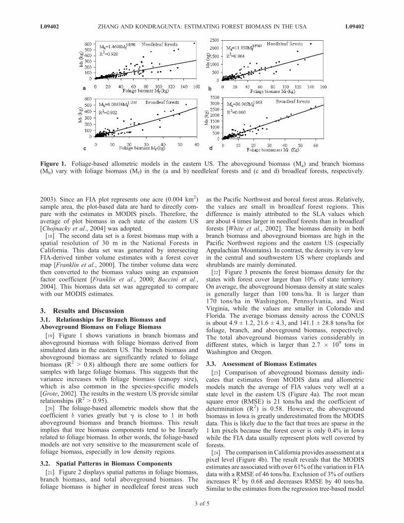
[19] Figure 1 shows variations in branch biomass andaboveground biomass with foliage biomass derived fromsimulated data in the eastern US. The branch biomass andaboveground biomass are significantly related to foliagebiomass (R2 > 0.8) although there are some outliers forsamples with large foliage biomass. This suggests that thevariance increases with foliage biomass (canopy size),which is also common in the species-specific models[Grote, 2002]. The results in the western US provide similarrelationships (R2 > 0.95).[20] The foliage-based allometric models show that the

coefficient d varies greatly but g is close to 1 in bothaboveground biomass and branch biomass. This resultimplies that tree biomass components tend to be linearlyrelated to foliage biomass. In other words, the foliage-basedmodels are not very sensitive to the measurement scale offoliage biomass, especially in low density regions.

3.2. Spatial Patterns in Biomass Components

[21] Figure 2 displays spatial patterns in foliage biomass,branch biomass, and total aboveground biomass. Thefoliage biomass is higher in needleleaf forest areas such

as the Pacific Northwest and boreal forest areas. Relatively,the values are small in broadleaf forest regions. Thisdifference is mainly attributed to the SLA values whichare about 4 times larger in needleaf forests than in broadleafforests [White et al., 2002]. The biomass density in bothbranch biomass and aboveground biomass are high in thePacific Northwest regions and the eastern US (especiallyAppalachian Mountains). In contrast, the density is very lowin the central and southwestern US where croplands andshrublands are mainly dominated.[22] Figure 3 presents the forest biomass density for the

states with forest cover larger than 10% of state territory.On average, the aboveground biomass density at state scalesis generally larger than 100 tons/ha. It is larger than170 tons/ha in Washington, Pennsylvania, and WestVirginia, while the values are smaller in Colorado andFlorida. The average biomass density across the CONUSis about 4.9 ± 1.2, 21.6 ± 4.3, and 141.1 ± 28.8 tons/ha forfoliage, branch, and aboveground biomass, respectively.The total aboveground biomass varies considerably indifferent states, which is larger than 2.7 � 109 tons inWashington and Oregon.

3.3. Assessment of Biomass Estimates

[23] Comparison of aboveground biomass density indi-cates that estimates from MODIS data and allometricmodels match the average of FIA values very well at astate level in the eastern US (Figure 4a). The root meansquare error (RMSE) is 21 tons/ha and the coefficient ofdetermination (R2) is 0.58. However, the abovegroundbiomass in Iowa is greatly underestimated from the MODISdata. This is likely due to the fact that trees are sparse in the1 km pixels because the forest cover is only 0.4% in Iowawhile the FIA data usually represent plots well covered byforests.[24] The comparison in California provides assessment at a

pixel level (Figure 4b). The result reveals that the MODISestimates are associated with over 61% of the variation in FIAdata with a RMSE of 46 tons/ha. Exclusion of 3% of outliersincreases R2 by 0.68 and decreases RMSE by 40 tons/ha.Similar to the estimates from the regression tree-based model

Figure 1. Foliage-based allometric models in the eastern US. The aboveground biomass (Ma) and branch biomass(Mb) vary with foliage biomass (Mf) in the (a and b) needleleaf forests and (c and d) broadleaf forests, respectively.


3 of 5

[Baccini et al., 2004], aboveground biomass is slightlyunderestimated for the areas where the biomass is larger than250 tons/ha. This discrepancy is likely attributed to the factorsincluding the sparse forests containing in MODIS pixels, thesaturation of MODIS estimates, and the representations ofdifferent years in MODIS and FIA data.

4. Conclusions

[25] The results in this study suggest that MODISdata combined with foliage-based allometric models providea robust tool to estimate biomass components acrosscontinental scales. Once the allometric models are wellestablished, they can be directly applied to calculate andupdate biomass data easily in regional and global areas.Moreover, this method produces not only commonly usedaboveground biomass, but also foliage biomass and branchbiomass. These components are particularly important forbiomass burning estimates.[26] The generalized foliage-based allometric models

indicate that foliage biomass accounts for more than 80%of variance in both branch biomass and abovegroundbiomass. On average, the forest biomass density acrossthe CONUS is 5, 22, and 141 tons/ha for foliage, branch,and aboveground trees, respectively. The abovegroundbiomass produced in this study matches field data sets verywell with an RMSE of 21 tons/ha on state average and40 tons/ha at pixel scales, although the time periods and themeasurement sizes in field data do not match those fromsatellite data.

[27] Acknowledgments. This research was supported by NOAAJoint Center for Satellite Data Assimilation. The authors wish to expresstheir thanks to Alessandro Baccini for providing biomass data in California,to Wenze Yang for help in preparing LAI data, to Maoshen Zhao fordiscussions and suggestions, and to Dan Tarpley and Felix Kogan forhelpful comments. The views, opinions, and findings contained in thoseworks are these of the author(s) and should not be interpreted as an officialNOAA or US Government position, policy, or decision.

Figure 4. Evaluation of aboveground biomass density(tons/ha) measured from MODIS land data using FIA data.(a) Sate level in the eastern US, (b) pixel level in theNational Forests in California.

Figure 2. Biomass (tons/ha) components derived fromMODIS land data and foliage-based generalized allometricmodels. (a) Foliage biomass, (b) branch biomass, and(c) aboveground biomass.

Figure 3. Average biomass density (foliage, branch, andaboveground) and percentage of forest-covered areas indifferent states.


4 of 5

ReferencesBaccini, A., M. A. Friedl, C. E. Woodcock, and R. Warbington (2004),Forest biomass estimation over regional scales using multisource data,Geophys. Res. Lett., 31, L10501, doi:10.1029/2004GL019782.

Brown, S. L., P. Schroeder, and J. S. Kern (1999), Spatial distribution ofbiomass in forests of the eastern USA, For. Ecol. Manage., 123, 81–90.

Brown, P. L., D. Doley, and R. J. Keenan (2000), Estimating tree crowndimension using digital analysis of vertical photographs, Agric. For.Meteorol., 100, 199–212.

Chojnacky, D. C., R. A. Mickler, L. S. Meath, and C. W. Woodall (2004),Estimates of down woody materials in eastern US forests, Environ.Manage., 33, S44–S55.

Dixon, R. K., R. A. Houghton, A. M. Solomon, M. C. Trexler, andJ. Wisniewski (1994), Carbon pools and flux of global forestecosystems, Science, 263, 185–190.

Dong, J. R., et al. (2003), Remote sensing estimates of boreal and temperateforest woody biomass: Carbon pools, sources, and sinks, Remote Sens.Environ., 84, 393–410.

Franklin, J., C. E. Woodcock, and R. Warbington (2000), Multi-attributevegetation maps of forest service lands in California supporting resourcemanagement decisions, Photogramm. Eng. Remote Sens., 66, 1209–1217.

Fraser, R. H., and Z. Li (2002), Estimating fire-related parameters in borealforest using SPOT VEGETATION, Remote Sens. Environ., 82, 95–110.

Friedl, M. A., et al. (2002), Global land cover mapping from MODIS:Algorithms and early results, Remote Sens. Environ., 83, 287–302.

Gholz, H. L., C. C. Grier, A. G. Campbell, and A. T. Brown (1979),Equations for estimating biomass and leaf area of plants in the PacificNorthwest, Res. Pap. 41, 39 pp., Oreg. State Univ., For. Res. Lab.,Corvallis, Oreg.

Grote, R. (2002), Foliage and branch biomass estimation of coniferous anddeciduous tree species, Silva Fennica, 36, 779–788.

Hansen, M. C., R. S. DeFries, J. R. G. Townshend, M. Carroll, andC. Dimiceli (2003), Global percent tree cover at a spatial resolutionof 500 meters: First results of the MODIS vegetation continuousfields algorithm, Earth Interact., 7, 1–15.

Heinsch, F. A., et al. (2003), User’s guide GPP and NPP (MOD17A2/A3)products NASA MODIS land algorithm, Sch. of For., Univ. of

Mont., Missoula, Mont. (Available at http://www.ntsg.umt.edu/modis/MOD17UsersGuide.pdf)

Ito, A., and J. E. Penner (2004), Global estimates of biomass burningemissions based on satellite imagery for the year 2000, J. Geophys.Res., 109, D14S05, doi:10.1029/2003JD004423.

Jenkins, J. C., R. A. Birdsey, and Y. Pan (2001), Biomass and NPP estima-tion for the mid-Atlantic region (USA) using plot-level forest inventorydata, Ecol. Appl., 11, 1174–1193.

Jenkins, J. C., D. C. Chojnacky, L. S. Heath, and R. Birdsey (2003),National-scale biomass estimators for United States tree species, For.Sci., 49, 12–35.

Lu, D. (2005), Aboveground biomass estimation using Landsat TM data inthe Brazilian Amazon, Int. J. Remote Sens., 26, 2509–2525.

Myneni, R. B., et al. (2002), Global products of vegetation leaf area andfraction absorbed PAR from year one of MODIS data, Remote Sens.Environ., 83, 214–231.

Paster, J., J. Aber, and J. M. Melillo (1984), Biomass prediction usinggeneralized allometric regressions for some Northeast tree species, For.Ecol. Manage., 7, 265–274.

Popescu, S. C., R. H. Wynne, and R. F. Nelson (2003), Measuring indivi-dual tree crown diameter with lidar and assessing its influence on esti-mating forest volume and biomass, Can. J. Remote Sens., 29, 564–577.

Ter-Mikaelian, M. T., and M. D. Korzukin (1997), Biomass equations forsixty-five North America tree species, For. Ecol. Manage., 97, 1–24.

White, M. A., P. E. Thornton, S. W. Runing, and R. R. Nemani (2002),Parameterization and sensitivity analysis of the BIOME_BGC TerrestrialEcosystem Model: Net Primary production controls, Earth Interact., 4,1–85.

Wirth, C., J. Schumacher, and E. Schulze (2004), Generic biomass func-tions for Norway spruce in Central Europe—A meta-analysis approachtoward prediction and uncertainty estimation, Tree Physiol., 24, 121–139.

��S. Kondragunta and X. Zhang, NOAA/NESDIS/ORA, 5200 Auth Road,

Camp Springs, MD 20746, USA. ([email protected]; [email protected])


5 of 5

Documents

Estimating forest biomass in the USA using generalized