A Very Brief Introduction to

Generalized Estimating

Equations

Gesine Reinert

Department of Statistics

University of Oxford

1. GEEs in the GLM context

Idea: extend generalized linear models (GLMs)

to accommodate the modeling of correlated

data

Examples: Whenever data occur in clusters

(panel data): Patient histories, insurance claims

data (collected per insurer), etc.

Often people would fit a linear model to such

data and only then adjust the standard errors

to account for the clustering; the problem is

that this post-hoc approach does not affect

the parameter estimates in the model. Instead

use GEEs:

GEE for GLMs in a nutshell:

1. Estimate a straightforward GLM, calculate

the matrix of scaling values.

2. The scaling matrix adjusts the Hessian in

the next iteration.

Each subsequent iteration updates the pa-

rameter estimates, the adjusted Hessian ma-

trix, and a matrix of scales.

The matrix of scales can be parametrized to

allow user control over the structure of depen-

dence in the data.

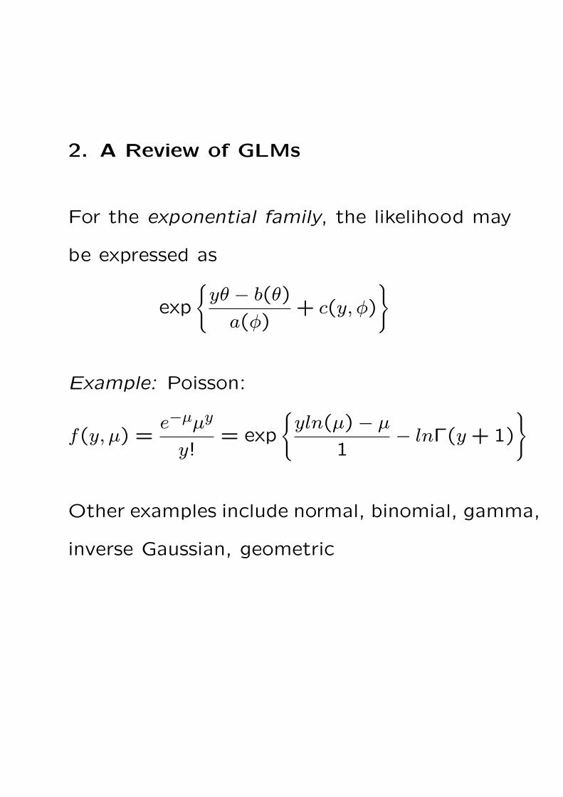
2. A Review of GLMs

For the exponential family, the likelihood may

be expressed as

exp

{yθ − b(θ)

a(φ)+ c(y, φ)

}

Example: Poisson:

f(y, µ) =e−µµy

y!= exp

{yln(µ)− µ

1− lnΓ(y + 1)

}

Other examples include normal, binomial, gamma,

inverse Gaussian, geometric

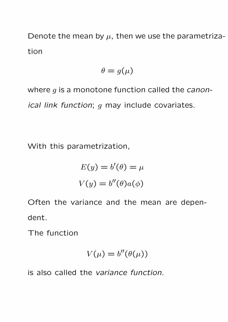
Denote the mean by µ, then we use the parametriza-

tion

θ = g(µ)

where g is a monotone function called the canon-

ical link function; g may include covariates.

With this parametrization,

E(y) = b′(θ) = µ

V (y) = b′′(θ)a(φ)

Often the variance and the mean are depen-

dent.

The function

V (µ) = b′′(θ(µ))

is also called the variance function.

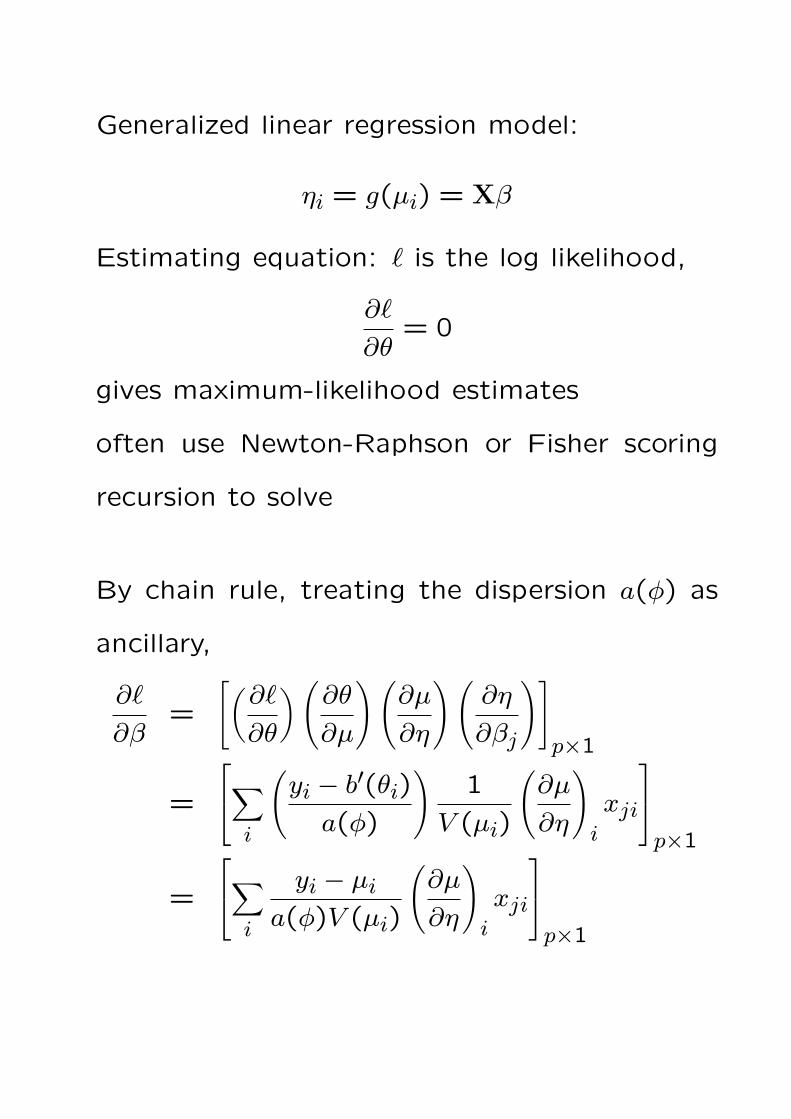
Generalized linear regression model:

ηi = g(µi) = Xβ

Estimating equation: ` is the log likelihood,

∂`

∂θ= 0

gives maximum-likelihood estimates

often use Newton-Raphson or Fisher scoring

recursion to solve

By chain rule, treating the dispersion a(φ) as

ancillary,

∂`

∂β=

[(∂`

∂θ

)(∂θ

∂µ

)(∂µ

∂η

)(∂η

∂βj

)]p×1

=

∑i

(yi − b′(θi)a(φ)

)1

V (µi)

(∂µ

∂η

)i

xji

p×1

=

∑i

yi − µia(φ)V (µi)

(∂µ

∂η

)i

xji

p×1

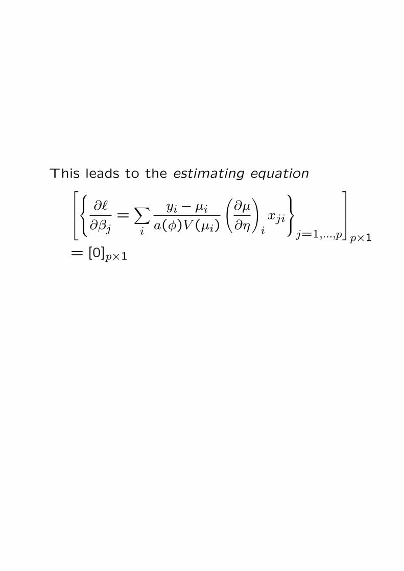
This leads to the estimating equation ∂`

∂βj=∑i

yi − µia(φ)V (µi)

(∂µ

∂η

)i

xji

j=1,...,p

p×1

= [0]p×1

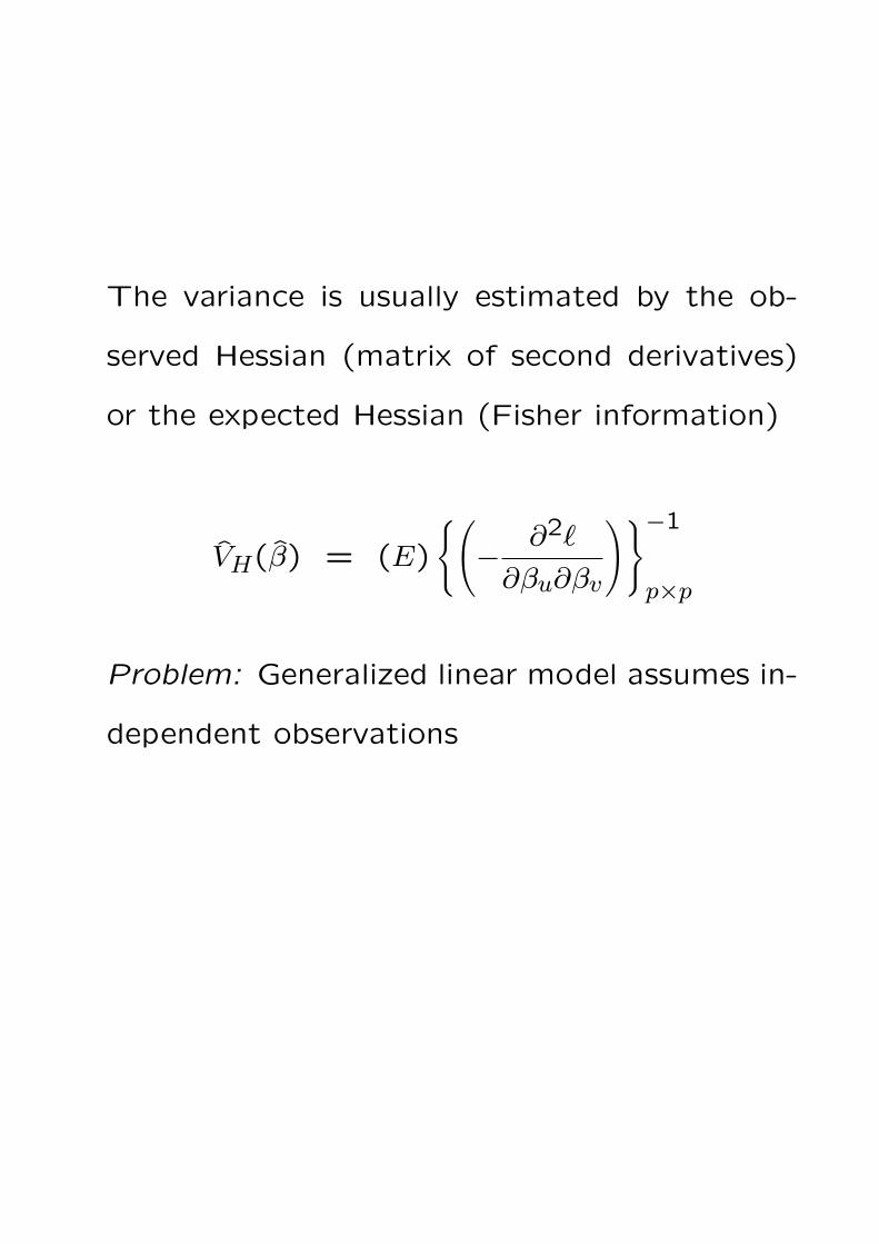
The variance is usually estimated by the ob-

served Hessian (matrix of second derivatives)

or the expected Hessian (Fisher information)

V̂H(β̂) = (E)

{(−

∂2`

∂βu∂βv

)}−1

p×p

Problem: Generalized linear model assumes in-

dependent observations

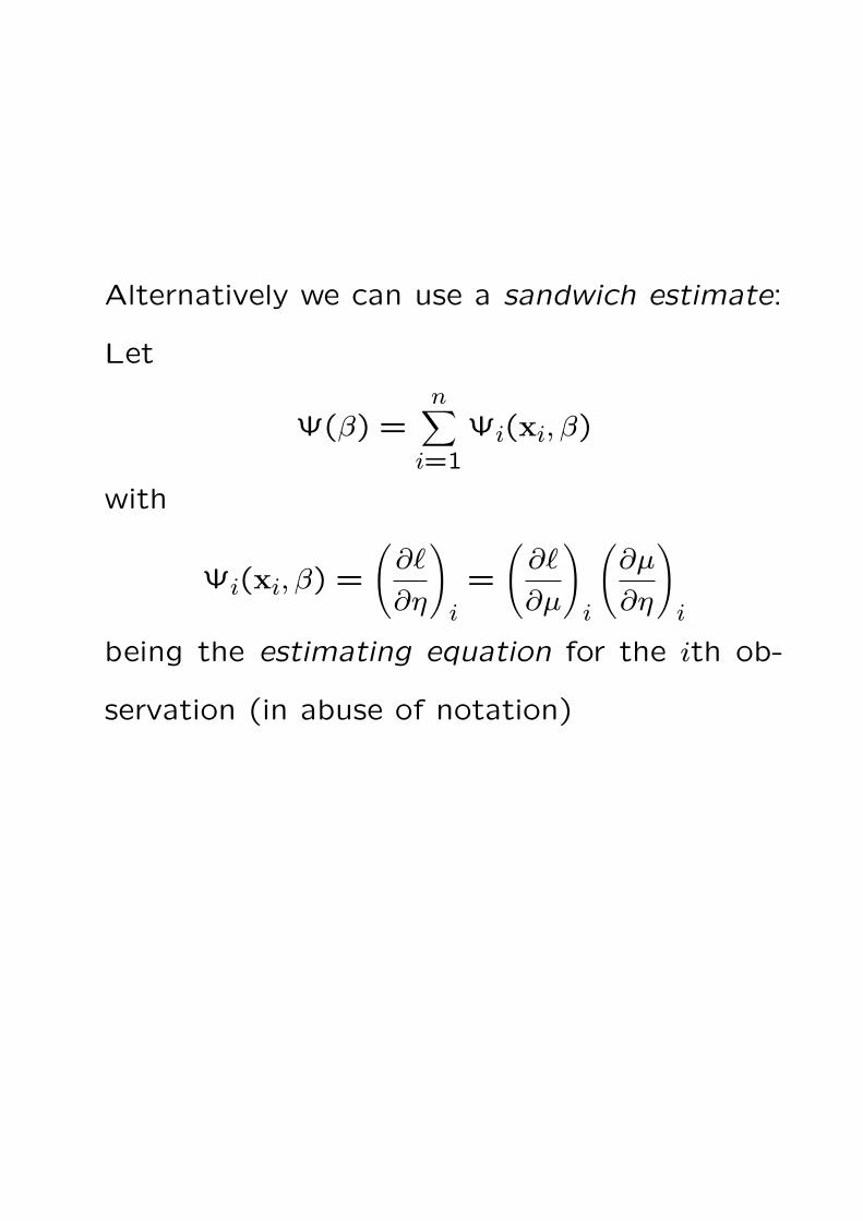
Alternatively we can use a sandwich estimate:

Let

Ψ(β) =n∑i=1

Ψi(xi, β)

with

Ψi(xi, β) =

(∂`

∂η

)i

=

(∂`

∂µ

)i

(∂µ

∂η

)i

being the estimating equation for the ith ob-

servation (in abuse of notation)

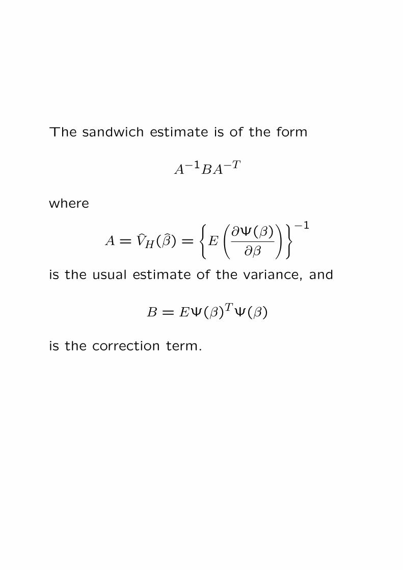
The sandwich estimate is of the form

A−1BA−T

where

A = V̂H(β̂) =

{E

(∂Ψ(β)

∂β

)}−1

is the usual estimate of the variance, and

B = EΨ(β)TΨ(β)

is the correction term.

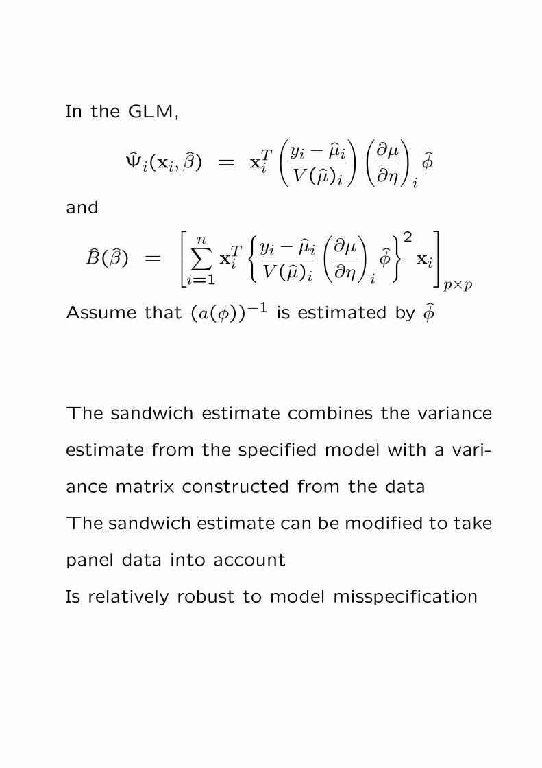
In the GLM,

Ψ̂i(xi, β̂) = xTi

(yi − µ̂iV (µ̂)i

)(∂µ

∂η

)i

φ̂

and

B̂(β̂) =

n∑i=1

xTi

{yi − µ̂iV (µ̂)i

(∂µ

∂η

)i

φ̂

}2

xi

p×p

Assume that (a(φ))−1 is estimated by φ̂

The sandwich estimate combines the variance

estimate from the specified model with a vari-

ance matrix constructed from the data

The sandwich estimate can be modified to take

panel data into account

Is relatively robust to model misspecification

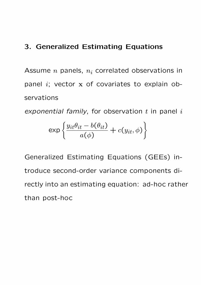
3. Generalized Estimating Equations

Assume n panels, ni correlated observations in

panel i; vector x of covariates to explain ob-

servations

exponential family, for observation t in panel i

exp

{yitθit − b(θit)

a(φ)+ c(yit, φ)

}

Generalized Estimating Equations (GEEs) in-

troduce second-order variance components di-

rectly into an estimating equation: ad-hoc rather

than post-hoc

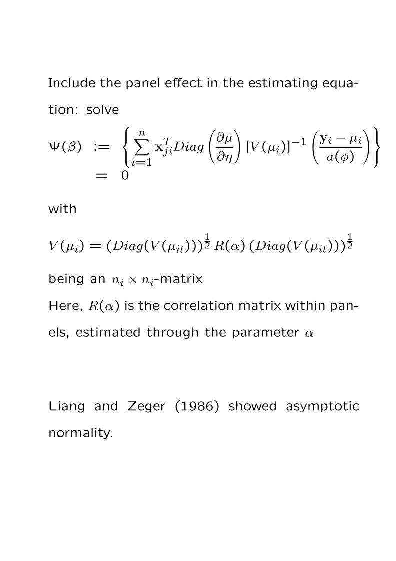
Include the panel effect in the estimating equa-

tion: solve

Ψ(β) :=

n∑i=1

xTjiDiag

(∂µ

∂η

)[V (µi)]−1

(yi − µia(φ)

)= 0

with

V (µi) = (Diag(V (µit)))12 R(α) (Diag(V (µit)))

12

being an ni × ni-matrix

Here, R(α) is the correlation matrix within pan-

els, estimated through the parameter α

Liang and Zeger (1986) showed asymptotic

normality.

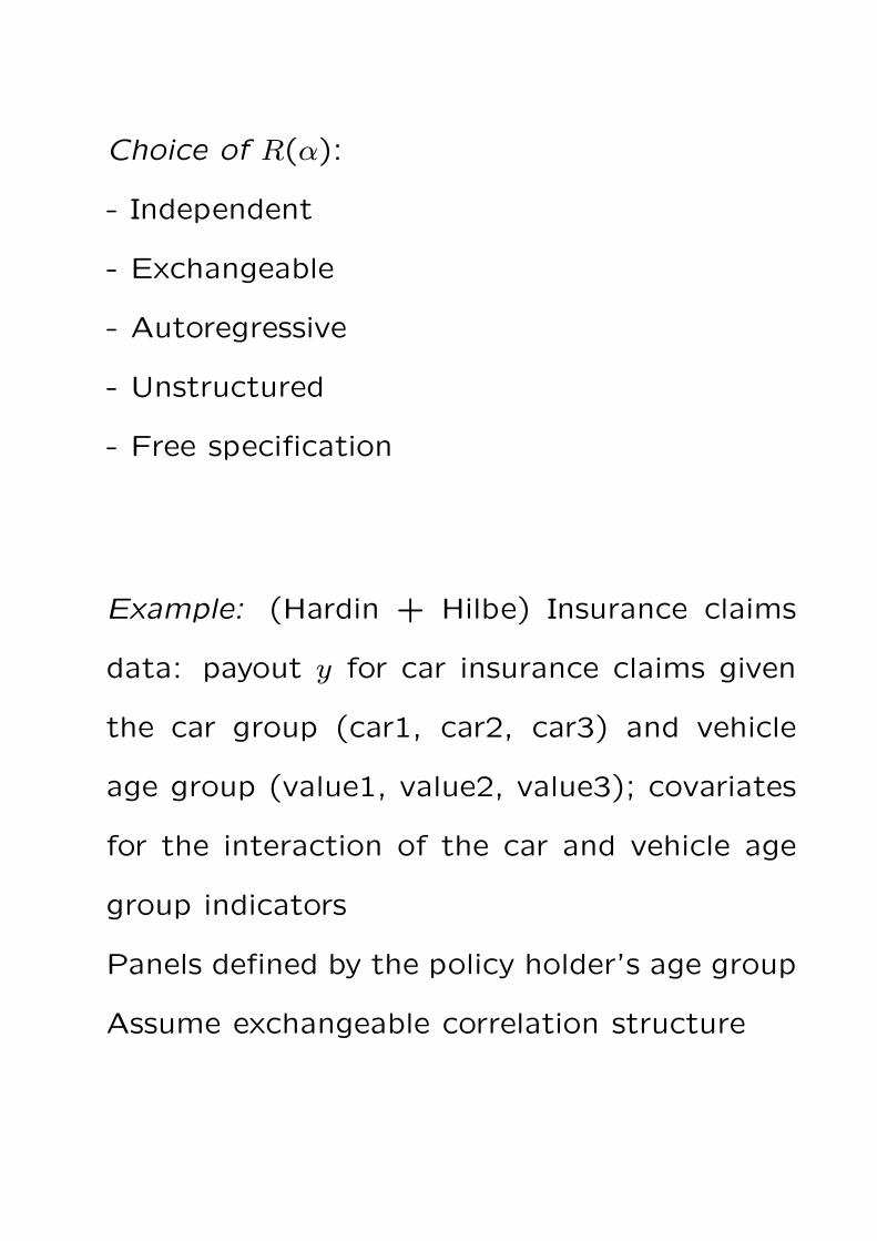
Choice of R(α):

- Independent

- Exchangeable

- Autoregressive

- Unstructured

- Free specification

Example: (Hardin + Hilbe) Insurance claims

data: payout y for car insurance claims given

the car group (car1, car2, car3) and vehicle

age group (value1, value2, value3); covariates

for the interaction of the car and vehicle age

group indicators

Panels defined by the policy holder’s age group

Assume exchangeable correlation structure

Population-averaged (PA) model: include the

within-panel dependence by averaging effects

over all panels

Subject-specific model: include subject-specific

panel-level components

Example: Subject-specific: estimate the odds

of a child having respiratory illnes if the mother

smokes compared to the odds of the same child

having respiratory illness if the mother does not

smoke

Population-averaged: estimate the odds of an

average child with respiratory illness and a smok-

ing mother to the odds of an average child with

respiratory illness and a nonsmoking mother.

Population-averaged models are often included

in statistical software (R, SAS, S-PLUS, Stata)

Subject-specific models require specification of

the randomness for each subject, and therefore

additional calculation and/or programming

4. Example: Geomorphological data

joint work with Stephan Harrison (Geography)

Certain landscape features are recorded in a

river valley and its tributary streams

The (circular) data for the valley come in stretches,

and are recorded both up-stream and down-

stream

There are 692 observations, 370 of these indi-

cate presence of the feature

The feature occurs in clumps; the longest clump

is of length 42

The data is decomposed into 6 stretches (pan-

els), the smallest has 45 observations, the largest

has 205 observations

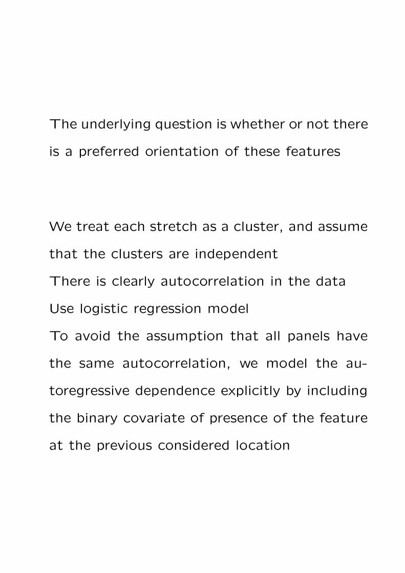
The underlying question is whether or not there

is a preferred orientation of these features

We treat each stretch as a cluster, and assume

that the clusters are independent

There is clearly autocorrelation in the data

Use logistic regression model

To avoid the assumption that all panels have

the same autocorrelation, we model the au-

toregressive dependence explicitly by including

the binary covariate of presence of the feature

at the previous considered location

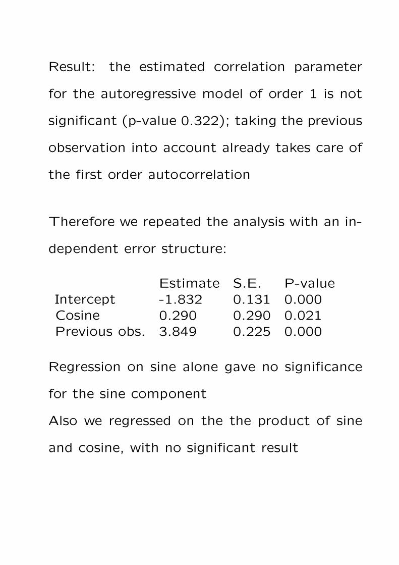
Result: the estimated correlation parameter

for the autoregressive model of order 1 is not

significant (p-value 0.322); taking the previous

observation into account already takes care of

the first order autocorrelation

Therefore we repeated the analysis with an in-

dependent error structure:

Estimate S.E. P-valueIntercept -1.832 0.131 0.000Cosine 0.290 0.290 0.021Previous obs. 3.849 0.225 0.000

Regression on sine alone gave no significance

for the sine component

Also we regressed on the the product of sine

and cosine, with no significant result

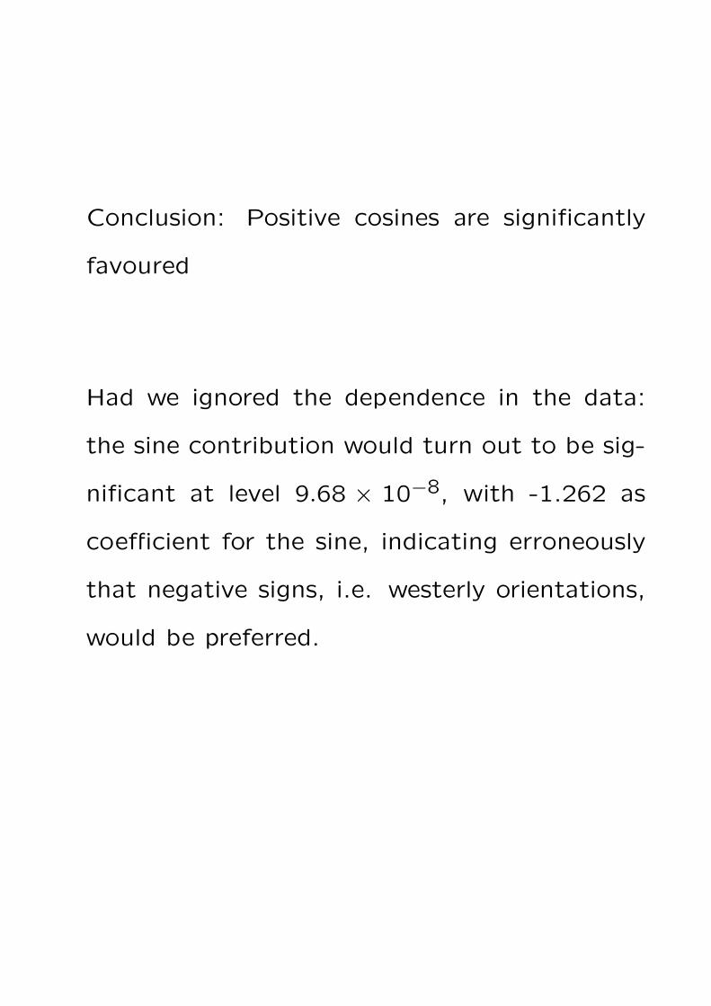
Conclusion: Positive cosines are significantly

favoured

Had we ignored the dependence in the data:

the sine contribution would turn out to be sig-

nificant at level 9.68 × 10−8, with -1.262 as

coefficient for the sine, indicating erroneously

that negative signs, i.e. westerly orientations,

would be preferred.

5. Last Remarks

One can use some working correlation struc-

ture that may be wrong, but the resulting re-

gression coefficient estimate is still consistent

and asymptotically normal; but selection of an

appropriate correlation structure improves effi-

ciency

There are further extensions of the model:

multinomial data

models where some covariates are measured

with error

robust version

missing data: under development

Residual analysis and tests for coefficients in

the model: available

References

Diggle, P.J., Heagerty, P., Liang, K.-Y., and Zeger, S.L.

(2002). Analysis of Longitudinal Data. Oxford Univer-

sity Press.

Godambe, V.P. ed. (1991). Estimating Functions. Ox-

ford University Press.

*Hardin, J.W. and Hilbe, J.M. (2003). Generalized Es-

timating Equations. Chapman and Hall, Boca Raton

etc.

Hosmer, D.W. and Lemeshow, S. (2000). Applied Lo-

gistic Regression. Second Edition. Wiley, New York

etc.

Liang, K.-Y. and Zeger, S. L. (1986). Longitudinal data

analysis using generalized linear models. Biometrika 73,

13–22.

(and references therein)