Estimating Dynamic Treatment Effects in Event Studies with

Heterogeneous Treatment Effects

Liyang Sun⇤and Sarah Abraham†

September 22, 2020

Abstract

To estimate the dynamic effects of an absorbing treatment, researchers often use two-way fixed

effects regressions that include leads and lags of the treatment. We show that in settings with variation in

treatment timing across units, the coefficient on a given lead or lag can be contaminated by effects from

other periods, and apparent pretrends can arise solely from treatment effects heterogeneity. We propose

an alternative estimator that is free of contamination, and illustrate the relative shortcomings of two-way

fixed effects regressions with leads and lags through an empirical application.

Keywords: difference-in-differences, two-way fixed effects, pretrend test

⇤Department of Economics, MIT, 77 Massachusetts Avenue, Cambridge, MA 02139. Corresponding author; lsun20@mit.edu.†Cornerstone Research, 699 Boylston St, Boston, MA 02116. The views expressed herein are solely those of the author, who is

responsible for the content, and do not necessarily represent the views of Cornerstone Research.

1 Introduction

Rich panel data has fueled a growing literature estimating treatment effects with two-way fixed effects re-

gressions. This body of applied work has prompted a corresponding econometrics literature investigating

the assumptions required for these regressions to yield causally interpretable estimates. For example, Athey

and Imbens (2018), Borusyak and Jaravel (2017), Callaway and Sant’Anna (2020a), de Chaisemartin and

D’Haultfœuille (2020) and Goodman-Bacon (2018) interpret the coefficient on the treatment status when

there is treatment effects heterogeneity and variation in treatment timing. Researchers are often also inter-

ested in dynamic treatment effects, which they estimate by the coefficients µ` associated with indicators for

being ` periods relative to the treatment, in a specification that resembles the following:

Y

i,t = ↵i +�t +’`

µ`1{t �E

i

= `}+�i,t . (1)

Here Y

i,t is the outcome of interest for unit i at time t, E

i

is the time when unit i initially receives the binary

absorbing treatment, and ↵i

and �t

are the unit and time fixed effects. Units are categorized into different

cohorts based on their initial treatment timing. The relative times ` = t�E

i

included in (1) cover most of the

possible relative periods, but may still exclude some periods.

The first goal of this paper is to uncover potential pitfalls associated with using the estimates of the

relative period coefficients µ` as “reasonable” measures of dynamic treatment effects. We decompose µ` to

show it can be expressed as a linear combination of cohort-specific effects from both its own relative period

` and other relative periods; unless strong assumptions regarding treatment effects homogeneity hold, the

terms that include treatment effects from other relative periods will not cancel out and will contaminate the

estimate of µ` . Importantly, this demonstrates that the widespread practice of using estimates of treatment

leads in (1) as a way of testing for parallel pretrends is problematic. Roth (2019), in his survey of the applied

literature, notes that checking whether µ` = 0 for ` leads of treatment is a common test for pretrends. Our

decomposition result implies that such a test would be invalid because the estimate of µ` is affected by both

pretrends and treatment effects heterogeneity, thus any test of µ` = 0 cannot accept or reject the existence of

pretrends without further assumptions on treatment effects.

We show how to calculate the weights underlying the linear combination of treatment effects in µ` using

an auxiliary regression. This auxiliary regression depends only on the distribution of cohorts and the relative

2

time indicators included in (1). Examining the weights allows researchers to gauge how large the amount

of treatment effects heterogeneity needs to be for µ` to be contaminated by treatment effects from other

relative periods. Our publicly-available Stata package eventstudyweights automates the estimation of these

weights using the panel dataset underlying any given specification of (1).

The second goal of this paper is to propose an alternative regression-based method that is more ro-

bust to treatment effects heterogeneity than regression (1). For dynamic treatment effects, researchers are

usually interested in estimating some average of treatment effects from ` periods relative to the treatment.

Our alternative method estimates the shares of cohort as weights. These weights are more interpretable

than the weights underlying regression (1) in the presence of treatment effects heterogeneity, and the re-

sulting weighted average of treatment effects extends beyond a convex combination of treatment effects

(Słoczynski, forthcoming). As discussed in Section 4.2, using the procedures of Callaway and Sant’Anna

(2020a), our alternative method can also accommodate covariates.

We illustrate both our decomposition results and our alternative method via an empirical application,

estimating the dynamic effects of a hospitalization. We follow Dobkin et al. (2018) in using the publicly-

available dataset, Health and Retirement Study (HRS), to first estimate two-way fixed effects regressions.

We then illustrate our alternative estimation method with this example. Among the outcomes studied by

Dobkin et al. (2018), we focus on out-of-pocket medical spending and labor earnings. Our alternative

method yields similar big-picture findings as the original paper that uses two-way fixed effects regressions:

the earnings decline due to hospitalization is substantial compared to the transitory out-of-pocket spending

increase. However, the two-way fixed effects estimates sometimes fall outside the convex hull of the un-

derlying effects. In contrast, estimates using our alternative method, by construction, are guaranteed to be

easy-to-interpret because they are weighted averages of the underlying effects, with weights corresponding

to cohort shares.

The rest of the paper is organized as follows. In the next subsection, we review the theoretical literature.

Section 2 formally introduces the event study design and discusses our definition in relation to the applied

literature. Section 3 derives the estimands of two-way fixed effects regression, and introduces sufficient

assumptions for them to be causally interpretable. Section 4 develops our alternative estimator. Section 5

illustrates our results using an empirical example and Section 6 concludes. All proofs are contained in the

Appendix.

3

1.1 Related Literature

This paper makes two main contributions within an active literature on the causal interpretations of two-

way fixed effects models in settings with staggered treatment adoption (Athey and Imbens, 2018; Borusyak

and Jaravel, 2017; Callaway and Sant’Anna, 2020a; de Chaisemartin and D’Haultfœuille, 2020; Goodman-

Bacon, 2018). Our paper is also related to the traditional literature analyzing non-separable panel and treat-

ment effects models e.g. Heckman et al., 1998, 1997; Blundell et al., 2004; Abadie, 2005; Chernozhukov et

al., 2013.

The first main contribution of our paper is to interpret estimates from two-way fixed effects specifications

when researchers include “dynamic” indicators for time relative to treatment and when treatment effects are

heterogeneous across adoption cohorts. We derive our results for a general class of two-way fixed effects

specifications where “dynamic” indicators can be flexibly specified as single relative periods ` or sets of

relative periods g (thus also capturing any “static” specification where all post-treatment indicators are

collected in a single set). This class of specifications encompasses all specifications addressed by Athey

and Imbens (2018), Borusyak and Jaravel (2017), Callaway and Sant’Anna (2020a), de Chaisemartin and

D’Haultfœuille (2020) and Goodman-Bacon (2018).

As a building block for the causal interpretation of estimates, we define CATT

e,` , the cohort average

treatment effects on the treated as the cohort-specific average difference in outcomes relative to never being

treated. Our choice of a “building block” is governed by the counterfactual and the type of heterogeneity

of interest. This object coincides with the “group-time average treatment effect” studied by Callaway and

Sant’Anna (2020a) and is more granular than the building block used by Goodman-Bacon (2018) that is an

average of CATT

e,` over some relative period range. Athey and Imbens (2018) consider an alternate coun-

terfactual to never being treated: being treated at a different time. Borusyak and Jaravel (2017) implicitly

assume away heterogeneity across cohorts within a relative period, so their building block reduces to ATT` .

de Chaisemartin and D’Haultfœuille (2020) allow for heterogeneous treatment paths within a cohort over

time across “groups”, thus their building block is at the group level. We defer a discussion of assumptions

underlying the causal interpretation of these building blocks to Section 2.

The second main contribution of our paper is to propose a simple regression-based alternative estimation

strategy that produces a more sensible estimand than conventional two-way fixed effects models under het-

erogeneous treatment effects. Our procedure is most similar to Callaway and Sant’Anna (2020a), but has the

4

following differences. First, in the setting where there is no never-treated group, our method uses the last co-

hort to be treated as a control group, whereas Callaway and Sant’Anna (2020a) use the set of not-yet-treated

cohorts. Our method and theirs thus rely on different, but non-nested parallel trends assumptions. Second,

our estimation method can be cast as a regression specification and thus may be more familiar to applied

researchers. However, a third difference is that the procedure of Callaway and Sant’Anna (2020a) allow for

conditioning on time-varying covariates. de Chaisemartin and D’Haultfœuille (2020) and Goodman-Bacon

(2018) respectively propose alternative estimators and diagnostic tools for estimation of causal effects in

staggered settings, but do not consider the estimation of the dynamic path of treatment effects as we do.

2 Event studies design

In this section we first formalize the “event studies design”. As discussed in Section 2.3, based on how this

term is deployed in the empirical literature, an event study design is a staggered adoption design where units

are treated at different times, and there may or may not be never treated units. It also nests a difference-in-

differences design, where units are either first treated at time t

0

or never treated.

Specifically, we consider a setting with a random sample of N units observed over T + 1 time periods,

where T is fixed. For each i 2 {0, . . .,N} and t 2 {0, ...,T}, we observe the outcome Y

i,t and treatment status

D

i,t 2 {0,1}: D

i,t = 1 if i is treated in period t and D

i,t = 0 if i is not treated in period t. Throughout we

assume that the observations {Yi,t,Di,t }T

t=0

are independent and identically distributed (i.i.d.).

In the general case of event studies we focus on an absorbing treatment such that the treatment status

over time is a non-decreasing sequence of zeros and then ones, i.e. D

i,s D

i,t for s < t. We can thus uniquely

characterize a treatment path by the time period of the initial treatment, denoted with E

i

=min

�t : D

i,t = 1

.

If unit i is never treated i.e. D

i,t = 0 for all t, we set E

i

=1. Based on when they first receive the treatment,

we can also uniquely categorize units into disjoint cohorts e for e 2 {0, . . .,T,1}, where units in cohort e are

first treated at the same time {i : E

i

= e}.

We define Y

e

i,t to be the potential outcome in period t when unit i is first treated in time period e. We

define Y

1i,t to be the potential outcome if unit i never receives the treatment, which we call the “baseline

outcome”. Since the timing of the initial treatment uniquely characterizes one’s treatment path, we can

5

represent the observed outcome for unit i as

Y

i,t = Y

E

i

i,t = Y

1i,t +

’0eT

(Y e

i,t �Y

1i,t ) ·1 {E

i

= e} . (2)

For any treatment that is not absorbing, if we replace the treatment status D

i,t with an indicator for

ever having received the treatment, the new treatment is absorbing by construction. Oftentimes the effect

of having ever received the treatment is of interest, as it captures the path of treatment effects even though

the treatment itself may be transient. For example, Deryugina (2017) is interested in the fiscal cost for a

county that has been hit by a hurricane. While a hurricane itself may be transient, the impact of having

had a hurricane may not be transient, hence why Deryugina (2017) codes the year of the first hurricane

experienced in a county as E

i

.

In the next section, we use the notation developed above to define the treatment effect of an event study

design.

2.1 Defining treatment effect of an event study design

In an event study design, we define the unit-level treatment effect as the difference between the observed

outcome relative to the never-treated counterfactual outcome: Y

i,t �Y

1i,t . Recall that Y

1i,t denotes the potential

outcome if unit i never receives the treatment. This particular counterfactual outcome Y

1i,t is a reasonable

“baseline outcome”, though other counterfactual outcomes may be of interest as well. For example, Athey

and Imbens (2018) also consider the treatment effect relative to the always-treated counterfactual outcome:

Y

i,t �Y

0

i,t . Sianesi (2004) defines the unit-level treatment effect to be relative to the not-yet-treated counter-

factual outcome: Y

i,t �Y

e

i,t for e > t.

When dynamic treatment effects are of interest, empirical researchers commonly report the coefficient

estimate bµ` associated with indicators for being ` periods relative to the treatment in regression (1) as an

estimate for the average lagged effect. To assess the causal interpretation of µ` , we need “building blocks”

for its decomposition, which are the average of unit-level treatment effects at a given relative period across

units first treated at time E

i

= e, i.e. units in the same cohort e. We call this average the cohort-specific

average treatment effects on the treated, formally defined below. Later in Section 3 we use them as building

blocks for the interpretation of the relative period coefficients µ` from two-way fixed effects regressions.

Definition 1. The cohort-specific average treatment effect on the treated (CATT) ` periods from initial

6

treatment is

CATT

e,` = E[Yi,e+` �Y

1i,e+` | E

i

= e]. (3)

Each CATT

e,` represents the average treatment effect ` periods from the initial treatment for the cohort

of units first treated at time e. We shift from calendar time index t to relative period index ` which denotes

the periods since treatment; for cohort e, ` ranges from �e to T � e because we observe at most e periods

before the initial treatment and T �e periods after the initial treatment. Relative periods allow us to compare

cohorts while holding their exposure to the treatment constant.

2.2 Identifying assumptions

With the above definitions, we formalize three potential identifying assumptions for outcomes of interest in

our event study design. The first assumption is a generalized form of a parallel trends assumption. The sec-

ond assumption requires no anticipation of the treatment. The third assumption imposes no variation across

cohorts. For each assumption, we first discuss its meaning and then compare it with similar assumptions

made in the literature interpreting two-way fixed effects regressions. Later in Section 3 we interpret the

relative period coefficients µ` from two-way fixed effects regressions under different combinations of these

assumptions.

Assumption 1. (Parallel trends in baseline outcomes.) For all s , t, the E[Y1i,t �Y

1i,s |Ei

= e] is the same for

all e 2 supp(Ei

).

If an application includes never-treated units so that 1 2 supp(Ei

), we need to especially consider

whether these never-treated units satisfy the parallel trends assumption. Never-treated units are likely to

differ from ever-treated units in many ways, and may not share the same evolution of baseline outcomes. If

the never-treated units are unlikely to satisfy the parallel trends assumption, then we should exclude them

from the estimation to avoid violation of this assumption.

While common in the applied literature, the parallel trends assumption is strong and oftentimes violated.

For example, Ashenfelter (1978) documented that participants in job training programs experience a decline

in earnings prior to the training period (Ashenfelter’s dip). The timing of job training is dependent on the

evolution of individual’s baseline earnings, and this scenario therefore does not satisfy the parallel trends

assumption. Proposition 1 is the only result in this paper derived without this assumption, but there is an

7

active literature studying inference under violations of the parallel trends assumption e.g. Rambachan and

Roth (2020).

Our parallel trends assumption coincides with that of de Chaisemartin and D’Haultfœuille (2020). One

could substitute this assumption with a different identifying assumption that baseline outcomes are mean

independent of E

i

i.e. at each t, E[Y1i,t |Ei

= e] is the same for all e 2 supp (Ei

) and in particular is equal to

E[Y1i,t ]. This stronger assumption is plausible when the timing of treatment is indeed randomized, which

is the assumption used by Athey and Imbens (2018). By taking the “fully dynamic” specification as their

DGP, Borusyak and Jaravel (2017) implicitly assume this version of a parallel trends assumption. Callaway

and Sant’Anna (2020a) propose a weaker version that is conditional on covariates. Finally, for a particular

estimand, Goodman-Bacon (2018) identifies a weaker version that only requires a weighted average of

E[Y1i,t �Y

1i,s |Ei

= e] (averaged across cohorts) to be zero.

Assumption 2. (No anticipatory behavior prior to treatment.) There is no treatment effect in pre-treatment

periods i.e. E[Y e

i,e+` �Y

1i,e+` | E

i

= e] = 0 for all e 2 supp(Ei

) and all ` < 0.

Assumption 2 requires potential outcomes in any ` periods before treatment to be equal to the baseline

outcome on average as in Malani and Reif (2015) and Botosaru and Gutierrez (2018). This is most plausible

if the full treatment paths are not known to units. If they have private knowledge of the future treatment path

they may change their behavior in anticipation and thus the potential outcome prior to treatment may not

represent baseline outcomes. For example, Hendren (2017) shows that knowledge of future job loss leads

to decreases in consumption. If the periods with anticipation behavior are known, then we may consider

an alternative version of Assumption 2, which holds for pre-periods in a subset of pre-treatment periods.

Depending on the application, it may still be plausible to assume no anticipation until K periods before the

treatment.

The no anticipation assumption proposed by Athey and Imbens (2018) is a deterministic condition which

stipulates that Y

e

i,e+` = Y

1i,e+` for all units i and e and ` < 0. By taking the “fully dynamic” specification as

their DGP, Borusyak and Jaravel (2017) allow anticipation by including pre-trends indicators in the DGP.

Callaway and Sant’Anna (2020a) and Goodman-Bacon (2018) implicitly assume no anticipation by using

observed outcomes in time periods before the initial treatment as the untreated potential outcomes.

Assumption 3. (Treatment effect homogeneity.) For each relative period `, CATT

e,` does not depend on

cohort e and is equal to ATT` .

8

Assumption 3 requires that each cohort experiences the same path of treatment effects. Treatment effects

need to be the same across cohorts in every relative period for homogeneity to hold, whereas for heterogene-

ity to occur, treatment effects only need to differ across cohorts in one relative period. The assumption of

treatment effect homogeneity is therefore strong, and in Section 3.4.1, we describe how it can be violated in

applied settings.

Our notion of treatment effect homogeneity does not preclude dynamic treatment effects; it only im-

poses that cohorts share the same path of treatment effects. The related literature sometimes formulates

restrictions on the dynamics of treatment effects as another notion of treatment effect homogeneity. Athey

and Imbens (2018) propose an assumption that “restricts the heterogeneity of the treatment effects over

time,” which implies CATT

e,` can vary over e but not over `. Borusyak and Jaravel (2017) refer to one

type of treatment effects heterogeneity as “only across the time horizon,” which implies CATT

e,` can vary

over ` but not over e. Callaway and Sant’Anna (2020a) allow for “arbitrary treatment effect heterogeneity”

when CATT

e,` varies across cohorts and over time. Similarly, de Chaisemartin and D’Haultfœuille (2020)

describe treatment effects that may be “heterogeneous across groups and over time periods.” Goodman-

Bacon (2018) allow heterogenous effects to either “vary across units but not over time” or “vary over time

but not across units.” The literature has not converged on a single notion of treatment effects heterogeneity

with time-varying treatment. Since researchers are interested in dynamic treatment effects when using a

“dynamic” specification, we do not restrict the path of treatment effects but rather use “heterogeneity” to

describe variation across cohorts only.

2.3 Relevance in the applied literature

To gauge the empirical relevance of our results, we survey the estimation methods used by the twelve papers

collected by Roth (2019) from three leading economics journals that contain the phrase “event study” in

their main text.1 From this sample of applied papers, we learn what specifications empirical researchers are

actually using when estimating two-way fixed effects regressions. Four papers in this sample consider the

simple setting where units either receive their first treatment at the same time or never receive the treatment.

The other eight papers in this sample consider the more complex setting where treated units receive their1We follow the selection criteria in Roth (2019): the original sample consists of 70 total papers, but is further constrained

to these twelve papers with publicly available data and code. The data and code are used to determine exactly the specification

estimated in these papers.

9

treatment at various times, and there may or may not be never treated units. This observation suggests an

event study in the applied literature nests two popular research designs: difference-in-differences design, but

also the design where units receive their first treatments at various times, which is our focus.2

2This setup is the same as the staggered adoption design proposed by Athey and Imbens (2018), but we keep the term event

study because it is common in the applied literature.

10

Tabl

e1:

Surv

eyof

App

lied

Pape

rs

Pape

rB

inar

yA

bsor

bing

Trea

tmen

t

Varia

tion

inTr

eatm

ent

Tim

ing

Pre-

Trea

tmen

tR

elat

ive

Perio

dEx

clud

ed

Excl

ude

Dis

tant

Rel

ativ

ePe

riods

Bin

Dis

tant

Rel

ativ

ePe

riods

Incl

udes

Nev

erTr

eate

dU

nits

Pane

lB

alan

ced

inR

elat

ive

Tim

e

Bos

chan

dC

ampo

s-Va

zque

z(2

014)

X

Fitz

patri

ckan

dLo

venh

eim

(201

4)G

alla

gher

(201

4)X

X-1

XX

Tew

ari(

2014

)X

X0

XU

jhel

yi(2

014)

XX

-1X

XB

aile

yan

dG

oodm

an-B

acon

(201

5)X

X-1

XX

X

Der

yugi

na(2

017)

XX

-1X

XX

Des

chên

eset

al.(

2017

)X

He

and

Wan

g(2

017)

XX

-1X

Lafo

rtune

etal

.(20

18)

XX

0X

XK

uzie

mko

etal

.(20

18)

XX

-1X

Mar

kevi

chan

dZh

urav

skay

a(2

018)

Notes:

This

tabl

eco

nsol

idat

eske

ypr

oper

tieso

fmai

nev

ents

tudy

spec

ifica

tions

acro

ssa

sam

ple

ofap

plie

dpa

pers

.We

follo

wth

ese

lect

ion

crite

riain

Rot

h(2

019)

:th

eor

igin

alsa

mpl

eco

nsis

tsof

70to

talp

aper

s,bu

tis

furth

erco

nstra

ined

toth

ese

twel

vepa

pers

with

publ

icly

avai

labl

eda

taan

dco

de.

The

data

and

code

are

used

tode

term

ine

exac

tlyth

esp

ecifi

catio

nes

timat

edin

thes

epa

pers

.We

focu

son

the

first

spec

ifica

tion

unde

rlyin

gth

eev

ent

stud

yes

timat

esin

each

pape

r,w

hich

we

view

asa

reas

onab

lepr

oxy

for

the

mai

nsp

ecifi

catio

nin

the

pape

r.N

ote

that

two

pape

rs(F

itzpa

trick

and

Love

nhei

m(2

014)

;Mar

kevi

chan

dZh

urav

skay

a(2

018)

)hav

eno

neof

the

attri

bute

slis

ted

inth

eco

lum

ns.

11

We summarize the main specifications in this sample of twelve applied papers in Table 1.3 The columns

of Table 1 collect key properties of these specifications. In Section 3.1, we introduce a general class of

specifications that encompasses all of these specification. The estimates for relative period coefficients µ`

from all these papers therefore fall under our analysis in the next section.

These papers demonstrated that event studies are used to address a broad range of research questions.

As an example of this literature, Bailey and Goodman-Bacon (2015) use the rollout of the first Community

Health Centers (CHCs) to study the longer-term health effects of increasing access to primary care. As

another example, Tewari (2014) uses variation in the timing of deregulation across states to estimate the

impact of financial development on homeownership.

3 Estimators from linear two-way fixed effects regression

We consider a two-way fixed effects (FE) regression of the following form, estimated on a panel of i =

1, . . .,N units for t = 0,1, . . .,T calendar time periods:

Y

i,t = ↵i +�t +’g2Gµg

1{t �E

i

2 g}+�i,t (4)

Here Y

i,t is the outcome of interest for unit i at time t, E

i

is the time for unit i to initially receive a binary

absorbing treatment, and ↵i

and �t

are the unit and time fixed effects. The set G collects disjoint sets g

of relative periods ` 2 [�T,T]. We allow some relative periods to be excluded from the specification and

denote the excluded set with gexcl = {` : ` <–g2G

g}. We denote by µg

the relative period coefficients from

regression (4), i.e. the population regression coefficients. Their corresponding OLS estimators are denoted

by bµg

respectively.

We are interested in the properties of µg

when there are variations in the initial treatment timing, and

there may or may not be never-treated units. Below in Section 3.1 we illustrate how the choice of G coincides

with a large number of specifications encountered in practice such as the “fully dynamic” specification. We

next decompose µg

in terms of CATT

e,` when various combinations of the three identifying assumptions fail.

For Propositions 1-3, we state the results in terms of the general specification (4). To specialize these results3We focus on the first specification underlying the event study estimates in each paper, which we view as a reasonable proxy

for the main specification in the paper.

12

to the “fully dynamic” specification (7), we note the corresponding decomposition would replace bins with

g = {`} for each relative period ` included in the specification and gexcl would contain all excluded relative

periods. The decomposition remains unchanged though the summation over ` 2 g simplifies since each g is

a singleton. For Proposition 4, the decomposition further simplifies for the “fully dynamic” specification as

discussed below.

Researchers may assume that µg

can be interpreted as a convex average of CATT

e,` for periods ` 2 g

from its corresponding set g; they may further assume the underlying weights have policy-relevant interpre-

tation, e.g. weights depending on proportions of cohorts. For example, Bailey and Goodman-Bacon (2015)

interpret them as “intention-to-treat effects” of the treatment in a given relative year. However, our results

show that µg

may not represent the parameter of interest without strong assumptions such as treatment ef-

fect homogeneity. Section 3.6 provides intuition for these negative results, and demonstrate the weights

are actually non-linear functions of proportions of cohorts. Section 3.7 illustrates how treatment effects

heterogeneity invalidates the pretrends test for a simple three-period setting.

3.1 Common specifications

Common specifications can be broadly categorized as either “static” or “dynamic”. Static specifications

estimate a single treatment effect that is time invariant. In contrast, dynamic specifications allow for non-

parametric changes in the treatment effects over time. Within dynamic specifications, researchers also need

to address issues of multi-collinearity, and may bin or trim distant relative periods. All of these choices can

be written as instances of (4) with the correct specification of G, meaning that our results are applicable for

a wide range of specifications employed in the empirical literature.

To clarify how to specify G in regression (4), we define D

`i,t B 1{t �E

i

= `} to be an indicator for unit i

being ` periods away from initial treatment at calendar time t. For never-treated units E

i

=1, we set D

`i,t = 0

for all ` and all t. We can represent the relative period bin indicator as

1{t �E

i

2 g} =’`2g

1{t �E

i

= `} =’`2g

D

`i,t . (5)

Static specification. For a “static” specification G contains a single element equal to g = [0,T]. The

indicator 1{t �E

i

2 g} is equivalent to an indicator for whether unit i has received its initial treatment by t:

13

1{E

i

t}. The “static” specification thus takes the following form

Y

i,t = ↵i +�t + µg’`�0

D

`i,t +�i,t (6)

and the corresponding set of excluded relative periods is gexcl = [�T,�1].

Dynamic specification. “Dynamic” specifications encompass any specifications of G where G contains

more than one element, thus treatment effects are allowed to vary over time non-parametrically. In its most

flexible form, a “fully dynamic” specification takes the following form

Y

i,t = ↵i +�t +�2’

`=�Kµ`D

`i,t +

L’`=0

µ`D

`i,t +�i,t (7)

and the corresponding set of excluded relative periods is gexcl = {�T, . . .,�K �1,�1, L+1, . . .,T}.

Excluding some relative periods from the “fully dynamic” specification is necessary to avoid multi-

collinearity, either among the relative period indicators D

`i,t , or with the unit and time fixed effects. For

example, when there are no never-treated units i.e. 1 < supp(Ei

) but with a panel balanced in calendar

time, we need to exclude at least two relative period indicators in G. These collinearities are discussed by

Borusyak and Jaravel (2017): one multi-collinearity comes from the relative period indicators summing to

one for every unitÕ

`2[�T,T ] D

`i,t = 1, and the other multi-collinearity comes from the linear relationship

between two-way fixed effects and the relative period indicators, namely t �E

i

= `.

Excluding relative periods close to the initial treatment is common in practice. Normalizing relative to

the period prior to treatment is the most common - six out of the eight papers we survey do so, as reflected

in the above specification where we drop D

�1

i,t . The remaining two papers exclude D

0

i,t .

Excluding distant relative periods is however less common (only one of the eight papers we survey

does so). Instead researchers “bin” or “trim” distant relative periods. For “binning”, researchers bin distant

relative periods into [�T,�K) and (L,T] and estimate a “binned” specification

Y

i,t = ↵i +�t + � ·’`<�K

D

`i,t +

�2’`=�K

µ`D

`i,t +

L’`=0

µ`D

`i,t +� ·

’`>L

D

`i,t +�i,t (8)

without excluding any distant relative periods so that gexcl = {�1}. For “trimming”, researchers trim their

panel to be balanced in relative periods.

14

Neither “binning” nor “trimming” resolves the issues of contamination discussed below (i.e. the pos-

sibility that treatment effects from other periods affect the estimate for a given µg

). We show the contam-

ination issue for the general specification (4) encompasses both practices. For a given coefficient in the

dynamic specification, “trimming” does however mechanically remove any treatment effects from the rela-

tive periods “trimmed” from the specification. For the static specification put forth in Borusyak and Jaravel

(2017), they noted that “trimming” also does not resolve the contamination issue they identified with the

static specification.

3.2 Interpreting the coefficients under no assumptions

First we show that without any assumptions, we can write µg

as a linear combination of differences in trends.

Proposition 1. The population regression coefficient on relative period bin g is a linear combination of

differences in trends from its own relative period ` 2 g, from relative periods ` 2 g0 belonging to other bins

g0 , g but included in the specification, and from relative periods excluded from the specification ` 2 gexcl:

µg

=’`2g

’e,1!g

e,`

⇣E[Y

i,e+` �Y

1i,0 |Ei

= e]�E[Y1i,e+` �Y

1i,0]

⌘(9)

+’

g

0,g,g02G

’`2g0

’e,1!g

e,`

⇣E[Y

i,e+` �Y

1i,0 |Ei

= e]�E[Y1i,e+` �Y

1i,0]

⌘(10)

+’

`2gexcl

’e,1!g

e,`

⇣E[Y

i,e+` �Y

1i,0 |Ei

= e]�E[Y1i,e+` �Y

1i,0]

⌘(11)

+’t

!g

1,t

⇣E[Y

i,t �Y

1i,0 |Ei

=1]�E[Y1i,t �Y

1i,0]

⌘. (12)

We use the superscript g to associate the weight !g

e,` with the coefficient µg

. The weight !g

e,` for e , 1

is equal to the population regression coefficient on 1{t �E

i

2 g} from regressing D

`i,t · 1 {E

i

= e} on all bin

indicators {1{t �E

i

2 g}}g2G included in the specification (4) and two-way fixed effects.

The above proposition is a direct result of regression mechanics. We provide an intuitive derivation for

the closed-form expressions for the weights using the classical “omitted variables bias formula” in Section

3.6. We defer the formal derivation to the Appendix. Here we mention the following properties of the

weights !g

e,` for e ,1.4

4We are grateful to Junyuan Chen of correcting the expression for !g1,t , weights for the never-treated units. Their expressions

and properties are not derived here because they are not the focus of our paper.

15

• For relative periods of µg

’s own bin i.e. ` 2 g, their associated weights as displayed in (9) sum to oneÕ

`2gÕ

e

!g

e,` = 1.

• For relative periods belonging to some other bin included in (4) i.e. ` 2 g0 for g0 , g and g0 2 G, their

associated weights as displayed in (10) sum to zeroÕ

`2g0Õ

e

!g

e,` = 0 for each bin g0.

• For relative periods not included in G, their associated weights as displayed in (11) sum to negative

oneÕ

`2gexcl

Õe

!g

e,` = �1.

We can easily estimate the weights !g

e,` for e , 1 for any given specification of G using the following

auxiliary regression:

D

`i,t ·1 {E

i

= e} = ↵i

+�t

+’g2G!g

e,`1{t �E

i

2 g}+u

i,t (13)

which regresses D

`i,t ·1 {E

i

= e} on all bin indicators included in regression (4) and two-way fixed effects.

All of the above properties can be extended to a case where covariates are added to regression (4) by

partialling out the covariates before proceeding. In other words, the terms in parentheses in (9), (10) and

(11) would be replaced by terms for which the covariates are partialled out. The weights can be estimated by

controlling for covariates in regression (13) the same way as they are controlled for in the original regression.

However, covariates complicate the interpretations of µg

in terms of CATT

e,` as we describe below

in Proposition 2-4. Depending on how covariates are controlled for in regression (4), we may need an

additional assumption that the counterfactual trends are linear in the time-varying covariates X

i,t . We leave

a full investigation of the introduction of covariates for future work.

3.3 Interpreting the coefficients under parallel trends assumption only

Proposition 2. Under Assumption 1 (parallel trends) only, the population regression coefficient on the

indicator for relative period bin g is a linear combination of CATT

e,`2g as well as CATT

e,`0 from other

relative periods `0 < g, with the same weights stated in Proposition 1:

µg

=’`2g

’e

!g

e,`CATT

e,` +’

g

0,g,g02G

’`02g0

’e

!g

e,`0CATT

e,`0 +’

`02gexcl

’e

!g

e,`0CATT

e,`0 . (14)

Under Assumption 1, the terms in Proposition 1 reduce to a linear combination of the causally inter-

16

pretable building blocks CATT

e,` as follows:

E[Yi,e+` �Y

1i,0 |Ei

= e]�E[Y1i,e+` �Y

1i,0] = CATT

e,` +E[Y1i,t �Y

1i,0 |Ei

]�E[Y1i,t �Y

1i,0]| {z }

=0

(15)

for t = e+ `. However, two issues for interpretability remain. First, the coefficient µg

can be written as an

average of not only CATT

e,` from own periods ` 2 g, but also CATT

e,`0 from other periods. Second, the

weights are still non-linear functions of the distribution of cohorts, same as those in (13), and they are not

restricted to lie in [0,1].

The properties of these weights as described following Proposition 1 imply that contamination from

other periods wanes once we impose restrictions on treatment effects. In the next two subsections we

illustrate how that can happen.

3.4 Interpreting the coefficients under parallel trends and no anticipation assumptions

Proposition 3. If Assumption 1 (parallel trends) holds and Assumption 2 (no anticipatory behavior in all

periods before the initial treatment) holds, the population regression coefficient µg

is a linear combination

of post-treatment CATT

e,`0 for all `0 � 0, with the same weights stated in Proposition 1:

µg

=’

`02g,`0�0

’e

!g

e,`0CATT

e,`0+’

g

0,g,g02G

’`02g0,`0�0

’e

!g

e,`0CATT

e,`0+’

`02gexcl,`0�0

’e

!g

e,`0CATT

e,`0 . (16)

Once we restrict pre-treatment CATT

e,`<0

to be zero under the no anticipatory behavior assumption,

the expression for µg

simplifies as terms involving CATT

e,`<0

drop out. However, the second term in the

expression for µg

remains unless we further impose treatment effect homogeneity for its summands to cancel

out each other. Thus, µg

may be non-zero for pre-treatment periods even if parallel trends holds.

This result immediately implies a shortcoming of using pre-treatment coefficients (i.e. µg

where g con-

tains only leads to the treatment ` < 0) to test for pretrends. Under the no anticipatory behavior assumption,

cohort-specific treatment effects prior to treatment are all zero: CATT

e,` = 0 for all ` < 0. Therefore, any

linear combination of these CATT

e,` is also zero. However, µg

is a function of post-treatment CATT

e,`0�0

as

well, even when g only contains elements with ` < 0. We revisit this implication in greater depth in Section

3.7. Callaway and Sant’Anna (2020a) provides alternative tests for pretrends that do not suffer from this

drawback.

17

3.4.1 Sources of treatment effect heterogeneity

Since treatment effects heterogeneity violates Assumption 3 and can alter how we interpret µg

, it is im-

portant to think through when different cohorts likely experience different paths of treatment effect. Such

heterogeneity could arise for many reasons. For example, cohorts may differ in their covariates, which af-

fect how they respond to treatment. We will explore a concrete example in our application: if treatment

effects differ with age, and there is variation in age across units first treated at different times, we will have

heterogeneous effects (see Section 5 for details). After controlling for covariates, cohorts may still vary

in their responses to the treatment if units select their initial treatment timing based on treatment effects.

This source of heterogeneity is still compatible with our parallel trends assumption, which only rules out

selection in the initial treatment timing based on the evolution of the baseline outcome. In addition to these

two sources of heterogeneity, treatment effects may vary across cohorts due to calendar time-varying effects

(e.g. macroeconomic conditions could govern the effects on labor market outcomes across cohorts).

3.5 Interpreting the coefficients under parallel trends and treatment effect homogeneity

Proposition 4. If Assumption 1 (parallel trends) holds and Assumption 3 (treatment effect homogeneity)

holds, then CATT

e,` = ATT` is constant across e for a given `, and the population regression coefficient µg

is equal to a linear combination of ATT`2g, as well as ATT`0<g from other relative periods:

µg

=’`2g!g

` ATT` +’g

0,g

’`02g0!g

`0 ATT`0 +’

`02gexcl

!g

`0 ATT`0 (17)

The weight !g

` =Õ

e

!g

e,` sums over the weights !g

e,` from Proposition 1, and is equal to the population

regression coefficient from the following auxiliary regression:

D

`i,t = ↵i +�t +

’g2G!g

` 1{t �E

i

2 g}+u

i,t (18)

which regresses D

`i,t on all bin indicators included in regression (4) and two-way fixed effects.

We note that even under treatment effect homogeneity µ` can still be contaminated by treatment effects

from the excluded periods. This contamination, however, can be avoided by adjusting the specification to

only exclude periods with zero treatment effect.

18

For specifications with relative time bins, we note that there can still be contamination from other bins as

suggested by the second term of expression (17). A sufficient condition to avoid such contamination would

be to group relative periods `0 into a bin only when their effects are the same since their weights !g

`0 would

sum to zero.

For the “fully dynamic” specification (7) where all g’s are singletons of relative time periods, the weight

!``0 is zero for each relative period `0 , ` that is included in the specification. The decomposition therefore

simplifies to

µ` = ATT` +’

`02gexcl

!``0 ATT`0 . (19)

3.6 Intuition for contamination

Proposition 3 demonstrates that even under the assumptions of parallel trends and no anticipation, estimates

µg

can still be contaminated by treatment effects from other periods. In this section we explain the intuition

behind why this contamination occurs for the “fully dynamic” specification (7). A decomposition of µ`

into a weighted average of CATT

e,`0 demonstrates that contamination is driven by the interaction of two

elements: the weights and CATT

e,`0. The weights underlying the contamination are non-linear functions of

the distribution of the cohorts. We do not attempt to provide a heuristic for determining the magnitude of

the weights, but instead describe how to estimate the weights and later on in Section 4 how to estimate each

CATT

e,` . This allows researchers to directly determine the degree of contamination in their application.

Our publicly-available Stata package eventstudyweights automates the estimation of these weights using the

panel dataset underlying any given specification of (1).

We apply the familiar omitted variable bias (OVB) formula to arrive at our decomposition. In an event

study where individuals receive the treatment at different times, the panel can never be balanced in both

calendar time and time relative to the initial treatment. As a result, the relative time indicators are still

correlated even after controlling for unit and time fixed effects in a two-way fixed effects regression. We use

the saturated regression and the OVB formula to illustrate how this correlation leads to contamination. We

defer its formal derivation to Appendix B.

Under the parallel trends assumption only, the saturated regression is

19

Y

i,t =’e

E[Y1i,0 | E

i

= e] ·1{E

i

= e}+’s

E[Y1i,s �Y

1i,0] ·1{t = s}

+’

`02gincl

’e2I 0

CATT

e,`0 ·⇣D

`0i,t ·1 {E

i

= e}⌘

+’

`02gexcl

’e2I 0

CATT

e,`0 ·⇣D

`0i,t ·1 {E

i

= e}⌘+ ✏

i,t (20)

where the regressors are cohort fixed effects, time fixed effects, and cohort-specific relative time indicators.

Furthermore, let gincl collect the relative time included in (7) and I = {e : 0 e+` T} collect the cohorts

that experience at least ` periods of treatment. The coefficient associated with the cohort-specific relative

time indicator D

`i,t · 1 {E

i

= e} is the cohort-specific average treatment effects CATT

e,` . To decompose the

coefficient µ` from (7) in terms of this saturated regression (20), the OVB formula multiplies the coefficients

in the saturated regression (20), CATT

e,`0, with the regression coefficients from (13), !`e,`0, which leads to

the following decomposition for µ` as a linear combination of CATT

e,`0:

µ` =’e,`0!`e,`0CATT

e,`0 . (21)

Since !`e,`0 is equal to a regression coefficient from (13), we can write it as

!`e,`0 = (�e, ·)|�e+`0 A

�1

` . (22)

Below we briefly comment on each of the three elements in the above expression to highlight how they

depend on the distribution of the cohorts. We defer their detailed definitions and derivations to Appendix

A.1.

• �e, · is a vector of the covariance between cohort e and the other cohorts, namely Cov (1{E

i

= e},1{E

i

= e

0}).

This term thus scales quadratically in the share of cohort e, and is small for small cohorts.

• �t

is a matrix of demeaned relative time indicators. The entry that corresponds to cohort e

0 and

relative time indicator D

`i,t is E[D`

i,t | E

i

= e

0]� 1

T+1

1 {e

0 2 I }. When T is large, i.e. the panel is long,

the second term is small and this entry is therefore approximately equal to the relative time indicator.

• A

�1

` is the row of A

�1 that corresponds to the relative time indicator D

`i,t for A the covariance matrix

20

of demeaned relative time indicators. Specifically, the entry in A that corresponds to the covariance

between demeaned D

`i,t and D

`0i,t is

’t

Cov⇣D

`i,t,D

`0i,t

⌘� 1

T +1

Cov (1 {E

i

2 I } ,1 {E

i

2 I 0}) . (23)

Within any time period D

`i,t and D

`0i,t are negatively correlated because no cohorts can be in these two

relative times at the same time. The second covariance term is in general also non-zero because being

in one cohort predicts (not) being in another cohort. Therefore A is in general not a diagonal matrix

and A

�1 would depend on the distribution of the cohorts non-linearly.

The three elements of (22) demonstrate the weights are non-linear functions of the distribution of the co-

horts, and they are in general non-zero. Nonetheless these weights can be estimated easily by the auxiliary

regression (13).

3.7 Invalidity of pretrend tests based on pre-period coefficients.

Contamination undermines the practice of testing for pretrends using pre-period coefficients. Proposition 3

implies that when effects are not homogenous across cohorts, it is problematic to interpret non-zero estimates

for µg

as evidence for pretrends, where the set g contains some leads ` < 0. Proposition 4 implies that even

with homogeneous treatment effect, if the effects associated with the excluded periods are not zero, then

contamination may still occur. Therefore without strong assumptions, pre-period coefficients should not be

used to test for pretrends because contamination can lead to estimates that are non-zero in the absence of

pretrends or zero in the presence of pre-trends.

Testing for pretrends using pre-period coefficients is commonly used in practice. As an example, He

and Wang (2017) mention “the estimated coefficients of the leads of treatments, i.e. �k

for all k �2

are statistically indifferent from zero” as evidence for lack of pretrends. As another example, Chetty et al.

(2014) assert “there is no trend toward higher individual pension contributions prior to year 0 ... as one would

expect if individuals’ tastes for saving were changing around the job switch” based on pre-period coefficient

estimates. These tests are only appropriate when the authors are willing to make strong assumptions.

To provide further intuition for why this test is not meaningful without additional assumptions we walk

through a simple example of the fully dynamic specification. Consider a balanced panel with T = 2 and

cohorts E

i

2 {1,2}. There are at least two multi-colinearities from including all four relative time indicators.

21

To form the fully dynamic specification we include gincl = {�2,0} and exclude gexcl = {�1,1}:

Y

i,t = ↵i +�t +’

`2{�2,0}µ`D

`i,t +�i,t . (24)

The choice of gexcl is based on the common practice of normalizing relative to the �1 period and distant

lags.

When there are no never treated units, we can express the pre-trend coefficient µ�2

in terms of CATTs:

µ�2

=CATT

2,�2| {z }own period

+1

2

CATT

1,0 �1

2

CATT

2,0| {z }`02gincl,`0,�2

+1

2

CATT

1,1 �CATT

1,�1

� 1

2

CATT

2,�1| {z }`02gexcl

(25)

It is apparent the weights maintain the structure described in Proposition 1. Without any anticipation effect,

the effects CATT

e,`<0

are zero and thus we expect µ�2

to be zero regardless of the cohort shares. With

homogeneous treatment effect, cohorts 1 and 2 experience the same treatment effect at relative time 0 so

that CATT

1,0 and CATT

2,0 cancel. But even with homogeneous treatment effect, the last term reflects the

role of excluded periods as CATT

1,�1

, CATT

2,�1

and CATT

1,1 receive non-zero weights. If there is any

lagged effect and CATT

1,1 is non-zero, the coefficient µ�2

would be non-zero even without any anticipation

effect. Note such behavior is independent of the distribution of the two cohorts.

22

Figure 1: Weight on CATT

e,`0 for `0 , �2 in the Coefficient µ�2

from Regression (24)

(a) Weight on CATT

e,0

(b) Weight on CATT

e,`0 for `0 2 {�1,1}

Notes: Panel (a) plots the weight on CATT

e,0 and panel (b) plots the weight on CATT

e,`0 for `0 2 {�1,1}under a given distribution of cohorts indexed by the x-axis. Specifically, we construct a panel balanced incalendar time with T = 2 and cohorts E

i

2 {1,2,1}. We vary the share of never-treated units Pr{E

i

=1}between [0,0.99] and divide the rest of the units evenly into cohorts treated at time 1 and 2. The x-axisindexes 1�Pr{E

i

=1}.

We can further introduce never treated units to our example to demonstrate how the weight !�2

e,`0 can

be non-linear in the distribution of cohorts while maintaining the structure described in Proposition 1. In

Figure 1 we plot the weights !�2

e,`0 as we vary the distribution of cohorts. Specifically, we vary the total share

of treated cohorts (shown on the x-axis), holding the shares of cohort 1 and 2 equal to each other and setting

the remaining to be the share of never treated units. For any distribution of cohorts, we have !�2

2,�2

= 1 (not

pictured). Panel (a) shows the weights for the included period `0 = 0 while panel (b) shows the weights for

the excluded periods `0 = �1 or 1.

23

The example shown in Figure 1 provides a visualization of three takeaways regarding the contamination

in the pre-trend coefficient µ�2

. First, both panels show that weights are a non-linear function of cohort

shares. Second, panel (a) confirms the structure for weights associated with `0 , ` but `0 2 gincl as described

in Proposition 1, namelyÕ

e

!�2

e,`0 = 0 for `0 , �2. However, these weights have non-zero magnitude. When

the effect is homogenous across cohorts, the contaminations are equal toÕ

e

!�2

e,`0 ATT`0 and cancel each

other out. In contrast, when effects are heterogeneous the different CATT

e,`0 will not necessarily cancel and

will contaminate the estimate for µ�2

. Third, panel (b) confirms the structure for weights associated with

excluded periods as described in Proposition 1, namelyÕ

e

!�2

e,`02gexcl

= �1. In other words, contaminations

from excluded periods can be thought of as a type of “normalization”: a weighted average of excluded

CATT

e,`0 is subtracted off the estimated treatment effect. However because these weights are not contained

in [0,�1], this average may lie outside of the convex hull of CATT

e,`0 for excluded periods. The latter issue

can be alleviated by an assumption that CATT

e,`0 are the same in all excluded periods; we can fully avoid

contamination from excluded period treatment effects by assuming all associated CATT

e,`0 are equal to zero.

4 Alternative estimation method

We propose a new estimation method that is robust to treatment effects heterogeneity. The goal of our

method is to estimate a weighted average of CATT

e,` for ` 2 g with reasonable weights, namely weights that

sum to one and are non-negative. In particular, we focus on the following weighted average of CATT

e,` ,

where the weights are shares of cohorts that experience at least ` periods relative to treatment, normalized

by the size of g:

⌫g

=1

|g |’`2g

’e

CATT

e,`Pr{E

i

= e | E

i

2 [�`,T � `]}. (26)

One can aggregate CATT

e,` to form other parameters of interest, such as those proposed by Callaway and

Sant’Anna (2020a). We focus on the above aggregation ⌫g

since our goal is to improve the non-convex and

non-zero weighting in µg

. The weights in ⌫g

are guaranteed to be convex and have an interpretation as the

representative shares corresponding to each CATT

e,` . Thus, our alternative estimator b⌫g

improves upon the

two-way fixed effects estimator bµg

by estimating an interpretable weighted average of CATT

e,`2g.

Our method proceeds by replacing each component in ⌫g

with its consistent estimator. We first estimate

each CATT

e,` using an interacted two-way fixed effects regression, then estimate the weight Pr{E

i

= e |

24

E

i

2 [�`,T � `]} using their sample analogs. In the final step, we average over the cohort-specific estimates

associated with relative period `. This method has a similar flavor as the method proposed by Gibbons et

al. (2019). They first use an interacted model to estimate the treatment effect for each fixed effect group;

the resulting group-specific estimates are averaged to provide the ATE. Their method improves fixed effects

regressions in a cross-sectional setting, and our method builds on theirs by improving two-way fixed effects

regressions in a panel setting. We therefore follow their terminology in calling our alternative estimator an

“interaction-weighted” estimator.

4.1 Interaction-weighted estimator

We describe the estimation procedure in three steps (with more detailed definitions stated in Definition 4 of

Appendix B).

Step 1. We estimate CATT

e,` using a linear two-way fixed effects specification that interacts relative

period indicators with cohort indicators, excluding indicators for cohorts from some set C:

Y

i,t = ↵i +�t +’e<C

’`,�1

�e,`(1{E

i

= e} ·D`i,t )+ ✏i,t . (27)

The exact specification depends on the cohort shares for a given application. If there is a never-treated

cohort, i.e. 1 2 supp{E

i

}, then we may set C = {1} and estimate regression (27) on all observations. If

there are no never-treated units, i.e. 1 < supp{E

i

}, then we may set C = {max{E

i

}}, i.e. the latest-treated

cohort and estimate regression (27) on observations from t = 0, . . .,max{E

i

}�1. Lastly, if there is a cohort

that is always treated, i.e. 0 2 supp{E

i

}, then we need to exclude this cohort from estimation.

The coefficient estimator b�e,` from regression (27) is a DID estimator for CATT

e,` with particular

choices of pre-periods and control cohorts. As DID is likely a familiar estimator for applied researchers, we

separate the more in-depth discussion of its definition, choices of pre-periods, and choices of control cohorts

in Section 4.2.

Step 2. We estimate the weights Pr{E

i

= e | E

i

2 [�`,T � `]} by sample shares of each cohort in the

relevant period(s) ` 2 g.

Step 3. To form our IW estimator, we take a weighted average of estimates for CATT

e,` from Step 1

25

with weight estimates from step 2. More formally, the IW estimator is

b⌫g

=1

|g |’`2g

’e

b�e,`cPr{E

i

= e | E

i

2 [�`,T � `]} (28)

where b�e,` is returned from step 1 and c

Pr{E

i

= e | E

i

2 [�`,T � `]} is the estimated weight returned from

step 2. We normalize the weights further by the size of g. If g is a singleton, then its size is |g | = 1.

Validity of the IW estimator. Under the parallel trends and no anticipation assumptions the coefficient

estimator b�e,` from regression (27) is a consistent estimator for CATT

e,` . The sample shares of each cohort

are also consistent estimators for the population shares. Thus, the IW estimator is consistent for a weighted

average of CATT

e,` with weights equal to the share of each cohort in the relevant period(s).

With a few standard assumptions, which we present as Assumption 4 in Appendix C, we show in Ap-

pendix C.1 that each IW estimator is asymptotically normal and derive its asymptotic variance. The large

sample approximation allows us to estimate the variance of IW estimators directly without relying on boot-

strapping as in Callaway and Sant’Anna (2020a). However, we only construct pointwise confidence interval

valid for a given IW estimator b⌫g

. The bootstrap-based inference by Callaway and Sant’Anna (2020a)

constructs simultaneous confidence intervals that are valid for the entire path of b⌫g

.

4.2 Difference-in-differences estimator for CATT

e,`

Definition 2. Assume cohort e is non-empty i.e.Õ

N

i=1

1{E

i

= e} > 0. Assume there exists some pre-period

s < e and some set of control cohorts C ✓ {c : e+ ` < c T} that are non-empty i.e.Õ

N

i=1

1{E

i

2 C} > 0.

Using the notion EN

to abbreviate the symbol 1

N

ÕN

i=1

, the DID estimator with pre-period s and control

cohorts C estimates CATT

e,` as

ˆ�e,` =

EN

[�Y

i,e+` �Y

i,s�·1 {E

i

= e}]EN

[1 {E

i

= e}] �EN

[�Y

i,e+` �Y

i,s�·1 {E

i

2 C}]EN

[1 {E

i

2 C}] . (29)

The assumption of non-empty cohort e, existence of pre-period and non-empty control cohorts makes

the DID estimator well-defined. For example, DID estimators for cohort 0 are not well-defined because a

pre-period does not exist for this cohort, which is why we exclude them from estimating regression (27) in

Step 1.

Using the above definition, in regression (27) from Step 1 of our proposed method, the coefficient

26

estimator b�e,` is a DID estimator for CATT

e,` with pre-period s = e�1 (because we exclude relative period

` = �1) and some choice of control cohorts C. If there is a never-treated cohort i.e. 1 2 supp{E

i

}, then

we set the control cohort to be never-treated units C = {1}. If there are no never-treated units, i.e. 1 <

supp{E

i

}, then we set the control cohort C = {max{E

i

}}, i.e. the latest-treated cohort. Among all possible

pre-periods, for regression (27) from step 1 of our proposed method we choose s = e�1 and C = {1} with

never-treated units (or {max{E

i

}} without never-treated units) because the resulting specification is a natural

extension of the common specifications of two-way fixed effects regression.

Note that without never-treated units we need to drop time periods t � max{E

i

} from estimating re-

gression (27) because every unit will be treated in these periods. The DID estimators for CATT

e,` for

e+` � max{E

i

} are thus not well-defined as the control cohort is empty C = ;. For example, when there are

just two cohorts with E

i

2 {1,T}, one treated at t = 1 and the other treated in the last period, we then need

to omit interaction terms involving the latest-treated cohorts as well as dropping observations from the last

period t = T from estimation.

Under some assumptions, this DID estimator b�e,` is an unbiased and consistent estimator for CATT

e,` ,

a fact that we build on in deriving the probability limit of the IW estimator. We state this in the following

proposition.

Proposition 5. If Assumptions 1 and 2 hold, then the DID estimator using any pre-period s < e and non-

empty control cohorts C is an unbiased and consistent estimator for CATT

e,` .

It is possible to relax the parallel trends assumption to allow the timing of treatment to depend on co-

variates. One can estimate CATT

e,` consistently based on the inverse propensity score reweighted estimator

proposed by Abadie (2005) and Callaway and Sant’Anna (2020a), the outcome regression approach by

Heckman et al. (1997), and the doubly robust estimator recently proposed by Sant’Anna and Zhao (2020).

The resulting estimates ˆ�e,l can then be plugged into step 3 to form our IW estimator. In particular, without

covariates and for the case with never treated units, our approach coincides with Callaway and Sant’Anna

(2020a). Therefore one can use the R package did developed by Callaway and Sant’Anna (2020b) to form

the IW estimator.

The choice of the pre-period s and the control cohorts C depends on the trade-off between relaxing As-

sumption 1 or Assumption 2. If Assumption 2 is likely to hold, we can choose any pre-period s < e and in-

clude not-yet-treated units in control cohorts C = {c : c > e+`} as in Callaway and Sant’Anna (2020a). This

27

choice allows us to relax the parallel trends assumption to be just E[Y1i,e+` �Y

1i,0 |Ei

= e] = E[Y1i,e+` �Y

1i,0 |Ei

>

e+`]. If instead we want to relax Assumption 2 to allow some anticipation, we then need the parallel trends

assumption to hold. For example, suppose we are only willing to assume away anticipation 2 periods before

a unit is treated, we may still be able to recover several CATT

e,` by appropriately selecting a pre-period and

a smaller set of control cohorts. We may choose any s < e�2 for the pre-period, and for control cohorts, we

may choose cohorts treated only after at least 2 periods from now C ✓ {c : e+ `+2 < c T}, or choose the

latest-treated cohort C = {max{E

i

}} as specified in regression (27).

5 Empirical Illustration

We illustrate our findings in the setting of Dobkin et al. (2018). Dobkin et al. (2018) study the economic

consequences of hospitalization, which is a large source of economic risk for adults in the United States. To

quantify these economic risks, in the first part of their analysis, Dobkin et al. (2018) leverage variation in

the timing of hospitalization observed in the publicly-available dataset, Health and Retirement Study (HRS),

which we describe in more detail in Section 5.1. Their estimation of the dynamic effects of hospitalization

using two-way fixed effects regressions provides a good context for demonstrating our results. As we argue

below in Section 5.2, parallel trends and no anticipation assumptions are plausible in this setting. However,

the effect of hospitalization is potentially heterogenous across individuals hospitalized in different years.

Our findings of non-convex and non-zero weighting would therefore apply to their two-way fixed effects

regression estimates, and our alternative estimator could lead to different estimates. Furthermore, this dataset

is publicly available, which allows us to provide replication files.

5.1 Data

Our sample selection closely follows Dobkin et al. (2018) but we include a cursory explanation here for com-

pleteness with an emphasis on how our final sample differs from their main analysis sample. Our primary

source of data is the biennial Health and Retirement Study (HRS). We identify the sample of individuals

who appear in two sequential waves of surveys and newly report having a hospital admission over the last

two years (the “index” or initial admission) at the second survey. To focus on health “shocks”, we restrict

attention to non-pregnancy-related hospital admissions as in Dobkin et al. (2018). We also follow Dobkin

et al. (2018) by focusing on adults who are hospitalized at ages 50-59.

28

Unlike Dobkin et al. (2018), we restrict our analysis to a subsample of these individuals who appear

throughout waves 7-11 (roughly 2004-2012). Our sample of analysis therefore includes HRS respondents

with index hospitalization during waves 8-11. The purpose of this sample restriction is to maintain a bal-

anced panel with a reasonable sample size.

Here i indexes an individual, and t indexes survey wave (T = 4) and is normalized to zero for wave 7,

the first wave in our sample. Among the outcomes Y

i,t studied by Dobkin et al. (2018), we focus on two:

out-of-pocket medical spending and labor earnings. They are derived from self-reports, adjusted to 2005

dollars and censored at the 99.95th percentile.

29

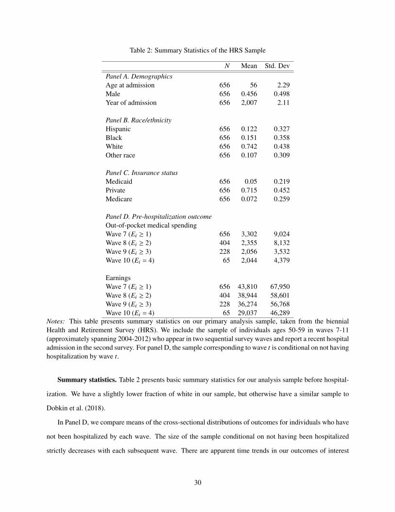
Table 2: Summary Statistics of the HRS Sample

N Mean Std. DevPanel A. Demographics

Age at admission 656 56 2.29Male 656 0.456 0.498Year of admission 656 2,007 2.11

Panel B. Race/ethnicity

Hispanic 656 0.122 0.327Black 656 0.151 0.358White 656 0.742 0.438Other race 656 0.107 0.309

Panel C. Insurance status

Medicaid 656 0.05 0.219Private 656 0.715 0.452Medicare 656 0.072 0.259

Panel D. Pre-hospitalization outcome

Out-of-pocket medical spendingWave 7 (E

i

� 1) 656 3,302 9,024Wave 8 (E

i

� 2) 404 2,355 8,132Wave 9 (E

i

� 3) 228 2,056 3,532Wave 10 (E

i

= 4) 65 2,044 4,379

EarningsWave 7 (E

i

� 1) 656 43,810 67,950Wave 8 (E

i

� 2) 404 38,944 58,601Wave 9 (E

i

� 3) 228 36,274 56,768Wave 10 (E

i

= 4) 65 29,037 46,289Notes: This table presents summary statistics on our primary analysis sample, taken from the biennialHealth and Retirement Survey (HRS). We include the sample of individuals ages 50-59 in waves 7-11(approximately spanning 2004-2012) who appear in two sequential survey waves and report a recent hospitaladmission in the second survey. For panel D, the sample corresponding to wave t is conditional on not havinghospitalization by wave t.

Summary statistics. Table 2 presents basic summary statistics for our analysis sample before hospital-

ization. We have a slightly lower fraction of white in our sample, but otherwise have a similar sample to

Dobkin et al. (2018).

In Panel D, we compare means of the cross-sectional distributions of outcomes for individuals who have

not been hospitalized by each wave. The size of the sample conditional on not having been hospitalized

strictly decreases with each subsequent wave. There are apparent time trends in our outcomes of interest

30

prior to hospitalization as we observe distributional changes across waves. Out-of-pocket medical spendings

fluctuate and earnings decrease with each wave on average as more individuals are retired in each subsequent

wave.

5.2 Setting

We illustrate how variations in the timing of hospitalization fit the event studies design proposed in Section 2.

We define treatment D

i,t to be ever having been hospitalized. In our terminology, we categorize individuals

into cohorts based on E

i

, which is defined as the survey wave of their initial hospitalization. Since we

restrict the sample to individuals who were ever hospitalized in waves 8-11, there are four cohorts E

i

2

{1,2,3,4}. Although hospitalization itself may not be an absorbing state, we are trying to model the impact

of having had any hospitalization. Thus, the cohort-specific average treatment effects CATT

e,` trace out

the path of treatment effects for cohort e following a negative health shock (even though the shock itself

may be transient), as opposed to never having been hospitalized. Next we discuss whether each of the three

identifying assumptions proposed is likely to hold in the context of unexpected hospitalizations.

Parallel trends (Assumption 1). Hospitalization is likely to be earlier among sicker individuals with

high out-of-pocket medical spending and low labor earnings. Thus, it is not plausible that the baseline

outcome Y

1i,t is mean independent of the timing of hospitalization. The parallel trends assumption is more

plausible as it allows the timing to depend on unobserved time-invariant characteristics such as chronic dis-

ease. Furthermore, hospitalized individuals might be on a downward trend for labor earnings already prior to

hospitalization compared to individuals who are never hospitalized. To reduce such confounding, we follow

Dobkin et al. (2018) to restrict the parallel trends assumption to individuals who were ever hospitalized.

No anticipatory behavior (Assumption 2). It is plausible that there is no anticipatory behavior prior

to the hospitalization, given that the treatment is restricted to conditions that are likely unexpected hospital-

izations. This assumption may be violated if individuals have private information about the probability of

these hospitalizations over time and thus adjust their behavior prior to hospitalization.

Treatment effect heterogeneity (Assumptions 3). For out-of-pocket medical spending, the effect of

hospitalization is potentially heterogenous across individuals hospitalized in different waves. Individuals

hospitalized in later waves are mechanically older at the time of hospitalization than individuals hospitalized

in earlier waves. The effect on out-of-pocket medical spending is largely determined by generosity of

health insurance, which may decrease as individuals age into Medicare. The effect on labor earnings is also

31

likely heterogenous as it depends on the labor market condition at the time of hospitalization: for example,

individuals hospitalized during the financial crisis may find it more difficult to return to the labor force, and

suffer a more grave decrease in earnings.

5.3 Illustrating weights in two-way fixed effects regression

We illustrate our results on two-way fixed effects regression by estimating the following specification with

indicators for up to three leads and lags following equation (3) of Dobkin et al. (2018)

Y

i,t = ↵i +�t + µ�3

D

�3

i,t + µ�2

D

�2

i,t + µ0

D

0

i,t + µ1

D

1

i,t + µ2

D

2

i,t + µ3

D

3

i,t +�i,t . (30)

For their estimation, Dobkin et al. (2018) trim their sample, keeping only observations up to three waves

prior to the hospitalization and three waves after the hospitalization, and weight their regression with survey

weights. To fully illustrate issues with this specification, we do not trim, but rather use a sample balanced in

calendar time for t 2 {0, . . .,4}, and do not apply survey weights. With a sample balanced in calendar time,

we need to exclude at least two relative period indicators due to multicollinearity. Following Dobkin et al.

(2018), we exclude the period right before hospitalization (` = �1). We also exclude ` = �4. Since we do

not trim, note that our results are not directly comparable to Dobkin et al. (2018) even though they are quite

similar.

We focus on a single coefficient µ�2

that is supposed to test for any pre-trend of hospitalizations. As in

Proposition 2, we can decompose µ�2

as

4’e=1

!�2

e,�2

CATT

e,�2

+’

`2{�3,0,1,2,3}

4’e=1

!�2

e,`CATT

e,` +’

`02{�4,�1}

4’e=1

!�2

e,`0CATT

e,`0 . (31)

As discussed in Proposition 1 we can estimate the underlying weights !�2

e,` by regressing 1 {E

i

= e} ·D`i,t on

the relative wave indicators included in specification (30) i.e. {D

`i,t }3

`=�3,,�1

and two-way fixed effects. The

coefficient estimator of D

�2

i,t in such regression, b!�2

e,` , consistently estimates !�2

e,` .

32

Figure 2: Estimated Weights b!�2

e,` Underlying µ�2

-.4-.2

0.2

.4W

eigh

ts

-4 -3 -2 -1 0 1 2 3Relative Wave

Weights on 1st cohort CATT Weights on 2nd cohort CATTWeights on 3rd cohort CATT Weights on 4th cohort CATT

Notes: The FE estimator for the pretrend of hospitalization bµ�2

estimates a linear combination of cohort-specific effects CATT

e,`’s from all cohorts e and relative waves ` as specified in equation (31). This figureplots the estimated weight b!�2

e,` associated with each CATT

e,` in this linear combination.

Figure 2 plots these estimated weights. As described in our decomposition results, these weights have

the following properties: (a) the four weights from relative wave ` =�2 sum to one; (b) the weights for other

included relative waves ` 2 {�3,0,1,2,3} sum to zero for each included relative wave; and (c) the weights

from excluded relative waves ` 2 {�4,�1} sum to negative one across these excluded relative waves.

The weights are non-negative for lags of treatments, which suggest that the FE estimate bµ�2

is partic-

ularly sensitive to estimates of the dynamic effects of hospitalizations and does not isolate the pre-trends.

Specifically, treatment effects heterogeneity in ` = �3,0,1,2 can affect the FE estimate bµ�2

. Applied re-

searchers can make similar plots to visualize the role of weights in their settings with our publicly-available

Stata package eventstudyweights by Sun (2020).

33

5.4 Comparing FE and IW estimates

We illustrate our alternative method (IW estimator) following the three steps outline in Section 4.1. First,

we estimate the interacted specification (27) as

Y

i,t = ↵i +�t +’

e2{1,2,3}

2’`=�3,,�1

�e,`1{E

i

= e} ·D`i,t + ✏i,t (32)

for t = 0, . . .,3. Specifically, we estimate CATT

e,` using a DID estimator b�e,` with pre-period s = �1 and

control cohort C = 4, the cohort hospitalized in the last period. This means we need to drop t = 4 from

estimation because everyone has been hospitalized by t = 4, and a control cohort for estimating CATT

e,` in

t = 4 does not exist. Second, we estimate the sample share of each cohort e across cohorts that experience

at least l periods relative to hospitalization by its sample analog. Third, we form IW estimates b⌫` by taking

weighted averages of b�e,` (returned from step one) with sample cohort share (returned from step two) as

weights.

34

Table 3: Estimates for the Effect of Hospitalization on Outcomes

(a) Out-of-pocket Medical Spending

FE IW CATT

e,`

` Wave Relative to Hospitalization bµ` b⌫` b�1,` b�

2,` b�3,`

-3 149 591 - - 591(792) (1273) (1273)

-2 203 353 - 299 411(480) (698) (967) (1030)

-1 0 0 0 0 0

0 3,013 2,960 2,826 3,031 3,092(511) (543) (1038) (704) (998)

1 888 530 825 107 -(664) (587) (912) (653)

2 1,172 800 800 - -(983) (1010) (1010)

3 1,914 - - - -(1426)

(b) Labor Earnings

FE IW CATT

e,`

` Wave Relative to Hospitalization bµ` b⌫` b�1,` b�

2,` b�3,`

-3 -2,642 -8,228 - - -8,228(3504) (6592) (6592)

-2 -5,089 -7,823 - -7,691 -7,964(3005) (4197) (6348) (4766)

-1 0 0 0 0 0

0 -1,225 -863 455 3,032 -7,107(2742) (2967) (5593) (4152) (5883)

1 -7,508 -5,435 -1,670 -10,826 -(4312) (4348) (6500) (4863)

2 -11,102 -10,670 -10,670 - -(5976) (6154) (6154)

3 -8,780 - - - -(8332)

Notes: This table reports three different sets of estimates for the dynamic effects of hospitalization on out-of-pocket medical spending in panel (a) and labor earnings in panel (b). The first column reports estimatesfrom the FE estimator bµ` . The sample includes observations from wave t = 0,1,2,3,4. Columns 3-5 reportthe estimates for CATT

e,` from b�e,` . The sample includes observations from wave t = 0,1,2,3. Column 2

reports the IW estimates which are constructed as the weighted average of b�e,`’s across cohorts e who are `

periods from hospitalization. Standard errors (clustered on the individual) are shown in parentheses.

In Table 3, we report the FE estimates bµ` and the IW estimates b⌫` , as well as the underlying CATT

e,`

estimates b�e,` . In this application, the FE estimates and IW estimates happen to be very similar in their

35

magnitude. The conclusion from Dobkin et al. (2018) based on FE estimates similar to ours still holds: we

find a substantial and persistent decline in the earnings due to hospitalization, and the increase in out-of-

pocket spending is transitory and small in comparison.

However, the FE estimates still suffer from non-convex and non-zero weighting as we show in Section

5.3, which can lead to interpretability issues depending on the amount of treatment effect heterogeneity.

Even though for both outcomes bµ0

falls in the convex hull of its underlying CATT

e,0 estimates, bµ�2

turns

out to be outside the convex hull of its underlying CATT

e,�2

estimates. In contrast, by construction, the IW

estimates b⌫` fall within the convex hull of its underlying CATT

e,` estimates and are unaffected by CATT

e,`0

estimates from other periods `0 , `. Thus, they have an interpretation as an average effect of the treatment

on the treated ` periods after initial treatment.

6 Conclusions

This paper analyzes the behavior of relative period coefficients µ` on the indicator for being ` periods away

from the treatment from two-way fixed effects regressions in settings with variation in treatment timing

and treatment effects heterogeneity. For dynamic treatment effects, researchers are usually interested in

estimating some average of treatment effects from ` periods relative to the treatment, and it is common

to report the coefficient estimate bµ` assuming that interpretation is valid. However, we show that in the

presence of heterogenous treatment effects, the coefficient µ` does not necessarily capture the dynamic

treatment effect as it can fall outside the convex hull of CATT

e,` from its corresponding period ` and may

pick up spurious terms consisting of treatment effects from periods other than `. This negative result is based

on the decomposition of the coefficients µ` as a linear combination of cohort-specific average treatment

effects on the treated CATT

e,` . The weights in the linear combination can be non-convex, and non-zero on

relative periods `0 , `.

Given these negative results on two-way fixed effects regression estimators, we propose “interaction-

weighted” (IW) estimators for estimating dynamic treatment effects. The IW estimators are formed by first

estimating CATT

e,` with a regression saturated in cohort and relative period indicators, and then averaging

estimates of CATT

e,` across e at a given `. These CATT

e,` are identified under parallel trends and no

anticipation assumptions. These estimators are easy to implement and robust to heterogenous treatment

effects across cohorts; the IW estimator associated with relative period ` is guaranteed to estimate a convex

36

average of CATT

e,` using weights that are sample share of each cohort e.

Finally, we illustrate the empirical relevance of our results by estimating the dynamic effect of hospi-

talization on the out-of-pocket medical spending and labor earnings using a setup similar to Dobkin et al.

(2018). We find non-convex and non-zero weights for two-way fixed effects regression in this example,

and show that the resulting estimates indeed sometimes fall outside the convex hull of the underlying CATT

estimates due to contamination by treatment effects from other relative periods. IW estimates, on the other

hand, are weighted averages of the underlying CATT estimates with weights representative of cohort share.

More broadly, our paper suggests that researchers can do more in this context to assess the validity of

underlying assumptions and how violations may impact their estimates. We demonstrate the sensitivity of

two-way fixed effects regressions to underlying assumptions and provide researchers with tools to assess

and address these issues. Specifically, for average treatment effects estimated using two-way fixed effects

regressions we recommend that empirical researchers directly estimate the underlying weights on cohort-

specific average treatment effects using our proposed auxiliary regressions. This exercise allows empirical

researchers to assess the degree of potential contamination under any assumed structure of treatment effects

heterogeneity. We also recommend empirical researchers consider estimation methods more robust to treat-

ment effects heterogeneity such as the IW estimator we propose. Developing additional tools for applied

researchers to identify and estimate interpretable parameters of interest is a promising avenue for future

research.

AcknowledgmentsWe are grateful to Isaiah Andrews, Amy Finkelstein, Anna Mikusheva, and Heidi Williams for their guidance and support. We

thank Alberto Abadie, Junyuan Chen, Jonathan Cohen, Nathan Hendren, Peter Hull, Guido Imbens, Yunan Ji, Sylvia Klosin,

Kevin Kainan Li, Paichen Li, Therese A. McCarty, Whitney Newey, James Poterba, Pedro H. C. Sant’Anna, Gergely Ujhe-

lyi and Helen Willis for helpful discussions. This research was supported by the National Institute on Aging, Grant Number

T32-AG000186. Replication code is available at http://economics.mit.edu/grad/lsun20/. The companion Stata package

eventstudyweights is available from the SSC repository.

Appendix

37

A Notation glossary and properties of double-demeaning

In this section, we provide relevant notations for proofs in Section B. Section A.1 introduces detailed ex-

pression for the weight.

We observe a balanced panel of N i.i.d. observations {{Yi,t,Di,t }T

t=0

}Ni=1

where Y

i,t 2 R is a real valued

outcome variable and D

i,t 2 {0,1} is a binary absorbing treatment status variable: D

i,t = 0 if i is not treated

in period t and D

i,t = 1 if i is treated in period t.

Since the treatment is absorbing, we can aggregate the treatment path {D

i,t }Tt=0

to a single discrete

random variable E

i

=min{t : D

i,t = 1}, which is the period of the initial treatment. Additionally, we define

D

`i,t B 1{t �E

i

= `} to be an indicator for being ` time periods relative to unit i’s initial treatment.

We focus on the following two-way fixed effects regression

Y

i,t = ↵i +�t +’g2Gµg

1{t �E

i

2 g}+�i,t

where g are disjoint sets of relative times, ↵i

and �t

are unit and time fixed effects.

Definition 3. For fixed T , consider a random vector {X

i,t }Tt=0

2 RT+1, jointly distributed according to P. At

each t, let ‹X

i,t denote the following random variable:

‹X

i,t = X

i,t �E[Xi,t ]�

1

T +1

T’s=0

X

i,s +1

T +1

T’s=0

E[Xi,s] (A.1)

The expectation E[Xi,t ] is taken cross-sectionally with respect to P at time t = 0, . . .,T .

Remark 1. Conventionally ‹X

i,t is referred to as the double-demeaned version of X

i,t , as it removes the

contemporaneous expectation E[Xi,t ] as well as the simple average across time for unit i, 1

T+1

ÕT

s=0

X

i,t . It

adds back a simple average across time of the expectations so that ‹X

i,t has the zero-mean and zero-sum

properties as detailed in Lemma 1.

Lemma 1. (Properties of double-demeaning.) For any

‹X

i,t and

‹Z

i,t , double-demeaned versions of X

i,t and

Z

i,t respectively, we have the following properties:

• zero-mean and zero-sum: E[ ‹Xi,t ] = 0 and

ÕT

t=0

‹X

i,t = 0;

• idempotent:Õ

T

t=0

E[ ‹Xi,t ‹Zi,t ] =

ÕT

t=0

E[Xi,t ‹Zi,t ] =

ÕT

t=0

E[ ‹Xi,tZi,t ];

• for any time-invariant random variables Z

i,t such that Z

i,t = Z

i

, double-demeaning annihilates it:

‹Z

i,t = 0.

38

Proof. The zero-mean and zero-sum properties hold by definition of double-demeaning:

E[ ‹Xi,t ] = E

"X

i,t �E[Xi,t ]�

1

T +1

T’s=0

X

i,s +1

T +1

T’s=0

E[Xi,s]

#(A.2)

= E[Xi,t ]�E[X

i,t ]�1

T +1

T’s=0

E[Xi,s]+

1

T +1

T’s=0

E[Xi,s] = 0 (A.3)

andT’t=0

‹X

i,t =

T’t=0

X

i,t �T’t=0

E[Xi,t ]�

T’t=0

1

T +1

T’s=0

X

i,s +

T’t=0

1

T +1

T’s=0

E[Xi,s] (A.4)

=

T’t=0

X

i,t �T’t=0

E[Xi,t ]�

T’s=0

X

i,s +

T’s=0

E[Xi,s] = 0 (A.5)

For the idempotent property, first note that by definition of double-demeaning, rearranging terms we can

write E[ ‹Xi,t ‹Zi,t ] as

= E

" X

i,t �1

T +1

T’s=0

X

i,s

!‹Z

i,t

#�E

" E[X

i,t ]�1

T +1

T’s=0

E[Xi,s]

!‹Z

i,t

#(A.6)

= E

" X

i,t �1

T +1

T’s=0

X

i,s

!‹Z

i,t

#�

E[X

i,t ]�1

T +1

T’s=0

E[Xi,s]

!·E[ ‹Z

i,t ] (A.7)

By the zero-mean property E[ ‹Zi,t ] = 0, the second term of the above expression is zero. Summing the first

term over t, we haveT’t=0

E[Xi,t ‹Zi,t ]�

T’t=0

E

" 1

T +1

T’s=0

X

i,s

!‹Z

i,t

#=

T’t=0

E[Xi,t ‹Zi,t ]�E[

1

T +1

T’s=0

X

i,s

!T’t=0

‹Z

i,t ] =T’t=0

E[Xi,t ‹Zi,t ]

(A.8)

where the last equality follows from the zero-sum propertyÕ

T

t=0

‹Z

i,t = 0. This provesÕ

T

t=0

E[ ‹Xi,t ‹Zi,t ] =Õ

T

t=0

E[Xi,t ‹Zi,t ]. Similarly we can show

ÕT

t=0

E[ ‹Xi,t ‹Zi,t ] =

ÕT

t=0

E[ ‹Xi,tZi,t ].

The annihilating property of double-meaning holds by definition for any time-invariant random variable.

Specifically, plugging in Z

i,t = Z

i

we have

‹Z

i,t = Z

i,t �E[Zi,t ]�

1

T +1

T’s=0

Z

i,s +1

T +1

T’s=0

E[Zi,s] (A.9)

= Z

i

�E[Zi

]� Z

i

+E[Zi

] = 0 (A.10)

⇤

39

A.1 Expression of the weight

In this section, we provide detailed definitions for the three elements in the expression of the weight !`e,`0 =

�0e, ·�e+`0 A

�1

` . Recall !`e,`0 is the weight associated with CATT

e,`0 in the linear combination underlying µ`:

!`e,`0 = e|`

T’t=0

E[ ‹Di,tD|

i,t ]!�1

| {z }B(A�1

` )|

T’t=0

E[ ‹Di,tD

`0i,t ·1 {E

i

= e}]

= (A�1

` )|T’t=0

Cov(Di,t �

1

T +1

T’t=0

Di,t,D

`0i,t ·1 {E

i

= e}� 1

T +1

T’t=0

D

`0i,t ·1 {E

i

= e})

= (A�1

` )|Pr {E

i

= e} ·⇣ �

E[Di,e+`0 �

1

T +1

T’t=0

Di,e+`0 | E

i

= e]��

�E[D

i,e+`0]�E[ 1

T +1

T’t=0

Di,e+`0]

� ⌘

= (A�1

` )|’e

0E[D

i,e+`0 �1

T +1

’t

Di,t | E

i

= e

0] ·Cov (1{E

i

= e},1{E

i

= e

0})

B (�e, ·)|�e+`0 A

�1

`

We note that

• The first term is the vector �e, · = (�e,e0)

e

02supp(Ei

) of the covariance between cohort indicators. Each

entry �e,e0 = Cov (1{E

i

= e},1{E

i

= e

0}) is the covariance between being in cohort e and being in

cohort e

0.

• The second term is the matrix �e+`0 of demeaned relative time indicators. The rows of the matrix are

indexed by cohorts e

0 2 supp(Ei

) and the columns of the matrix are indexed by relative time indicators

included in the specification (7). The entry that corresponds to cohort e

0 and relative time indicator

D

`i,t is E[D`

i,e+`0 �1

T+1

Õt

D

`i,t | E

i

= e

0]. Note that the sumÕ

t

D

`i,t is equal to 1 {E

i

2 I } the indicator

for whether this individual ever experience the relative time `.

• The third term is the row vector of A

�1 that corresponds to the relative time indicator D

`i,t . Here

A is the covariance matrix of demeaned relative time indicators included in the specification (7).

Specifically, the entry that corresponds to the covariance between demeaned D

`i,t and D

`0i,t is’

t

Cov

D

`i,t �

1

T +1

’t

D

`i,t,D

`0i,t �

1

T +1

’t

D

`0i,t

!.

Plugging inÕ

t

D

`i,t = 1 {E

i

2 I } gives the expression in the main text.

40

B Proofs of decomposition results

Proof of Proposition 1

Proof. Collect the relative time indicators in a column vector Di,t = (1{t �E

i

2 g})|g2G . Collect their cor-

responding coefficients in a column vector µ = (µg

)|g2G . Partialling out the unit and time fixed effects,

Regression (4) is

‹Y

i,t = µ| ‹D

i,t +�i,t (B.1)

where ‹X

i,t is time- and cross-sectional demeaned version of X

i,t as defined in Definition 3. By the idempotent

property of Lemma 1

µg

= e|g

T’t=0

E[ ‹Di,tD|

i,t ]!�1

T’t=0

E[ ‹Di,tYi,t ] (B.2)

where eg

is a column vector with one in the entry corresponding to the entry of 1{t � E

i

2 g} in Di,t , and

zero otherwise.

To further develop the expression for the population regression coefficients µg

, we note that by Lemma

1, we haveÕ

T

t=0

E[ ‹Di,tY

1i,0] =

ÕT

t=0

E[Di,t ‹Y1

i,0] = 0 since Y

1i,0 is time-invariant, and E[ ‹D

i,t ] = 0 by the zero-

mean property.T’t=0

E[ ‹Di,tYi,t ] =

T’t=0

E[ ‹Di,tYi,t ]�

T’t=0

E[ ‹Di,tY

1i,0]

| {z }=0

=

T’t=0

E[ ‹Di,t

⇣Y

i,t �Y

1i,0

⌘] =

T’t=0

E[ ‹Di,tE[Y

i,t �Y

1i,0 |Ei

]]

(B.3)

=

T’t=0

E[ ‹Di,tE[Y

i,t �Y

1i,0 |Ei

]]�T’t=0

E[ ‹Di,t ]| {z }

=0

E[Y1i,t �Y

1i,0] (B.4)

=

T’t=0

E[ ‹Di,t

⇣E[Y

i,t �Y

1i,0 |Ei

]�E[Y1i,t �Y

1i,0]

⌘]. (B.5)

We can abbreviate the term in the parentheses as f (Ei

, t) to emphasize it is a function of E

i

and t. Since E

i

41

and t take on discrete values, we can write

E[Yi,t �Y

1i,0 |Ei

]�E[Y1i,t �Y

1i,0]C f (E

i

, t) =1’e=0

f (e, t) ·1 {E

i

= e} (B.6)

=

T’e=0

T’`=�T

f (e, e+ `) ·1{t � e = `} ·1 {E

i

= e}+ f (1, t) ·1 {E

i

=1}

(B.7)

=

T’`=�T

T’e=0

D

`i,t1 {E

i

= e} · f (e, e+ `)+ f (1, t) ·1 {E

i

=1} . (B.8)

Even though we sum over e 2 {0, . . .,1}, if there are no never-treated units (or no units in a particular cohort

e

0), then we have no units take on values E

i

=1 (or E

i

= e

0). The range of the summation is therefore still

sensible. Note that we replace 1{t � e = `} ·1 {E

i

= e} with D

`i,t ·1 {E

i

= e} because for E

i

,1,

D

`i,t ·1 {E

i

= e} = 1{t �E

i

= `} ·1 {E

i

= e} = 1{t � e = `} ·1 {E

i

= e} . (B.9)

Using the above expression, the coefficient µg

can be written as

µg

=e|g

T’t=0

E[ ‹Di,tD|

i,t ]!�1

T’t=0

T’`=�T

T’e=0

E[ ‹Di,tD

`i,t ·1 {E

i

= e}] f (e, e+ `) (B.10)

+ e|g

T’t=0

E[ ‹Di,tD|

i,t ]!�1

T’t=0

E[ ‹Di,t1 {E

i

=1}] f (1, t) (B.11)

=’l2g

T’e=0

e|g

T’t=0

E[ ‹Di,tD|

i,t ]!�1

T’t=0

E[ ‹Di,tD

`i,t ·1 {E

i

= e}]

| {z }=!g

e,`

f (e, e+ `) (B.12)

+’g

0,g

’`2g0

T’e=0

e|g

T’t=0

E[ ‹Di,tD|

i,t ]!�1

T’t=0

E[ ‹Di,tD

`i,t ·1 {E

i

= e}]

| {z }=!g

e,`

f (e, e+ `) (B.13)

+’

`2gexcl

T’e=0

e|g

T’t=0

E[ ‹Di,tD|

i,t ]!�1

T’t=0

E[ ‹Di,tD

`i,t ·1 {E

i

= e}]

| {z }=!g

e,`

f (e, e+ `) (B.14)

+

T’t=0

e|g

T’t=0

E[ ‹Di,tD|

i,t ]!�1

E[ ‹Di,t1 {E

i

=1}]

| {z }=!g

1, t

f (1, t). (B.15)

The superscript g in !g

e,` indexes µg

. The subscript ` in !g

e,` indexes f (e, e+ `). The expression above

the braces makes it clear that the weight !g

e,` is equal to the population regression coefficient on 1{t �E

i

2

g} from regressing D

`i,t · 1 {E

i

= e} on all the bin indicators i.e. {1{t � E

i

2 g}}g2G and two-way fixed

42

effects included in (4). This proves Proposition 1. We next show several properties of these weights in the

expression of µg

:

To see that 1)Õ

`2gÕ

T

e=0

!g

e,` = 1, the sum of weights is equal to’`2g

T’e=0

!g

e,` =’`2g

T’e=0

e|g

T’t=0

E[ ‹Di,tD|

i,t ]!�1

T’t=0

E[ ‹Di,tD

`i,t ·1 {E

i

= e}] (B.16)

=e|g

T’t=0

E[ ‹Di,tD|

i,t ]!�1

T’t=0

E[ ‹Di,t

’`2g

D

`i,t ·

T’e=0

1 {E

i

= e}] (B.17)

=e|g

T’t=0

E[ ‹Di,tD|

i,t ]!�1

T’t=0

E[ ‹Di,t1{t �E

i

2 g}] (B.18)

where in the last line we note D

`i,t = 0 for E

i

= 1 by construction. It is thus the population regression

coefficient on 1{t�E

i

2 g} from regressing 1{t�E

i

2 g} on Di,t and the unit and time fixed effects, which is

just one. Similarly, for each g0 , g, the sum of weights is the population regression coefficient on 1{t �E

i

2

g0} from regressing 1{t �E

i

2 g} on Di,t and the unit and time fixed effects, which is zero. To see that the

weights from all excluded relative time add up to negative one across cohorts, note that the sum of these

weights is equal to’

`2gexcl

T’e=0

!g

e,` =e|g

’`2gexcl

T’t=0

E[ ‹Di,tD|

i,t ]!�1

T’t=0

E[ ‹Di,tD

`i,t ] (B.19)

=e|g

T’t=0

E[ ‹Di,tD|

i,t ]!�1

T’t=0

E

h‹Di,t

’`2gexcl

D

`i,t

i(B.20)

=e|g

T’t=0

E[ ‹Di,tD|

i,t ]!�1

T’t=0

E[ ‹Di,t

�1 {E

i

,1}�’g2G

’`2g

D

`i,t

�] (B.21)

=� e|g

T’t=0

E[ ‹Di,tD|

i,t ]!�1

T’t=0

E[ ‹Di,t

’g2G

’`2g

D

`i,t ] (B.22)

=� e|g

’g2G

T’t=0

E[ ‹Di,tD|

i,t ]!�1

T’t=0

E[ ‹Di,t1{t �E

i

2 g}] = �1 (B.23)

where the third equality follows fromÕ

`2gexcl

D

`i,t +

Õg2G

Õ`2g D

`i,t =

Õ�T `T D

`i,t = 1 {E

i

,1}. The

fourth equality follows from the properties of double-demeaning proved in Lemma 1. The last line simplifies

to negative one because each term in the summation T’t=0

E[ ‹Di,tD|

i,t ]!�1

T’t=0

E[ ‹Di,t1{t �E

i

2 g}] (B.24)

equals the population regression coefficient on Di,t from regressing 1{t � E

i

2 g} on Di,t and the unit and

time fixed effects, which is a column vector with one in the entry corresponding to 1{t �E

i

2 g}. Summing

43

over g, the above expression is equal to a column vector of ones. ⇤

Proof of Proposition 2

Proof. Under the parallel trends assumption, we can replace each term in Proposition 1 with

E[Yi,e+` �Y

1i,0 |Ei

= e]�E[Y1i,e+` �Y

1i,0] = CATT

e,` +E[Y1i,t �Y

1i,0 |Ei

= e]�E[Y1i,t �Y

1i,0]| {z }

=0

(B.25)

for t = e+ `. Furthermore, we have E[Yi,t �Y

1i,0 |Ei

=1]�E[Y1i,t �Y

1i,0] = 0 for the never-treated units. ⇤

Proof of Proposition 3

Proof. Under the no anticipation assumption, set the corresponding terms to zero in the linear combination

displayed in Proposition 2. ⇤

Proof of Proposition 4

Proof. Under the assumption of homogeneous treatment effect, we have CATT

e,` = ATT` for all e. This

simplifies Proposition 2 to’`2g

’e

!g

e,`

!ATT` +

’g

0,g

’`2g0

’e

!g

e,`

!ATT` +

’`2gexcl

’e

!g

e,`

!ATT` . (B.26)

Recall the weight !g

e,` is equal to the population regression coefficient on 1{t � E

i

2 g} from regressing

D

`i,t · 1 {E

i

= e} on all the bin indicators, i.e. {1{t �E

i

2 g}}g2G and two-way fixed effects included in (4).

Summing over e would imply the weight !g

` BÕ

e

!g

e,` is equal to the population regression coefficient on

1{t�E

i

2 g} from regressing D

`i,t on all the bin indicators, i.e. {1{t�E

i

2 g}}g2G and two-way fixed effects

included in (4). ⇤

C Supplementary results related to IW estimator

In this section, we first provide detailed definition for the IW estimator, and then state its asymptotic behav-

ior. We then prove its asymptotic normality and derive its asymptotic variance in Section C.1.

Definition 4. The IW estimator for ⌫g

, a weighted average of CATT

e,`2g is constructed via the following

three steps. We focus on the setting without never-treated units, using pre-period s = �1 and the last-treated

cohort as the control cohort C = {max{E

i

}}. The setting with never-treated units can be defined similarly

by modifying the interacted specification.

44

Step 1 Estimate the CATT

e,` using the interacted specification.

Y

i,t = ↵i +�t +’

e,max{Ei

}

’`,�1

�e,`(1{E

i

= e} ·D`i,t )+ ✏i,t (C.1)

= ↵i

+�t

+B|i,t�+ ✏i,t (C.2)

on observations from t = 0, . . .,max{E

i

}�1 and E

i

, 0. We need to drop time period beyond max{E

i

}

because DID estimators for CATT

e,` for e+ ` � max{E

i

} do not exist as explained in the main text.

We need to exclude cohort 0 from estimation because DID estimators for CATT

0,` do not exist as ex-

plained in the main text. Note that among regressors we exclude interactions with 1{E

i

= max{E

i

}}

and we exclude interactions with D

�1

i,t . Here Bi,t is a column vector collecting the interactions

1{E

i

= e} · D

`i,t . Similarly, � is a column vector collecting the coefficients �

e,` on 1{E

i

= e} · D

`i,t .

The matrix notation is used later to derive the asymptotic variance of IW estimators.

Step 2 Estimate the weights, which are cohort shares among cohorts that experience at least ` periods of

treatment relative to the initial treatment.

Denote by N

e

BÕ

N

i=1

1 {E

i

= e} the number of units in cohort e. Denote by h

` = {e : 1� ` e

max{E

i

}�1� `} to be the set of cohorts that experience at least ` periods of treatment relative to the

initial treatment. Below vec (A) vectorizes matrix A by stacking its columns.

Definebf` to be a matrix with its (t, e)th entry equal to 1 {t � e = `} · N

e

/Õe2h` N

e

. Here 1 {t � e = `}

indicates when cohort e experiences exactly ` periods of treatment and N

e

/Õe2h` N

e

is equal to the

sample share of units in cohort e among units that experience at least l periods of treatment. Denote

by f` the probability limit ofbf` , which is a matrix with its (t, e)th entry equal to 1 {t � e = `} ·Pr{E

i

=

t � l | E

i

2 h

`}. For example, with E

i

2 {0,1,2,3} for T = 3 and ` = 0, we have h

0 = {1,2} and thus

bf0 =©≠≠´

N

1

N

1

+N2

0

0

N

2

N

1

+N2

™Æƨ

(C.3)

and its probability limit is

f0 =©≠≠´

Pr {E

i

= 1|1 E

i

2} 0

0 Pr {E

i

= 2|1 E

i

2}

™Æƨ. (C.4)

In proof below, we show that the weight matrix estimatorbf` is asymptotically normalp

N(vec(bf`)�vec(f`))!

d

N(0,⌃f

` ).

Step 3 Compute the IW estimator as the weighted sum of b�e,` (estimated in Step 1) using weights (estimated

45

in Step 2).

To form an estimator alternative to the dynamic FE estimator bµg

from Regression (4), we can use

b⌫g

B1

|g |’`2g

’e2h`

N

eÕe2h` N

e

b�e,` =

1

|g |’`2g

vec(bf`)|b�. (C.5)

With a few standard assumptions (which we present together below as Assumption 4) on Regression

(27), we can show that the IW estimators are asymptotically normal.

Assumption 4. (The saturated regression assumptions).

1. There are observations from at least two cohorts that are not treated in t = 0.

2. Independent, identically distributed cross-sectional observations: {(Ei

,Yi

) : i = 1,2, . . .,N} are i.i.d.

draws from their joint distribution where Yi

= (Yi,0, . . .,Yi,T )| is a T ⇥1 vector.

3. Large outliers are unlikely: (Bi,t, ✏i,t ) have nonzero finite fourth moments.

4. Denote by

‹B the data matrix, whose rows consist of

‹B|i,t , double-demeaned version of B|

i,t . Assume

‹B has full rank. If

‹B is reduced-rank because cohort e is empty, then discard regressors involving

1{E

i

= e}.

Denote by � the probability limit of b�, which is a vector of CATT

e,` . We next state the asymptotic

distribution of the IW estimators specifically for ⌫` , the average effect at relative time `. Results for the

more general case of ⌫g

, which is the average effects across relative times ` 2 g, can be derived similarly.

Note that we use a clustered variance-covariance structure to allow the possibility that Y

i,t are dependent

across t due to serial correlation.

Proposition 6. (Consistency and asymptotic normality of the IW estimators for ⌫`). Under the assumptions

of Proposition 5 and Assumption 4, the IW estimator converges in probability to

b⌫` !p

’e2h`

Pr

�E

i

= e | E

i

2 h

`

CATT

e,` = vec(f`)|�. (C.6)

The asymptotic distribution of this estimator is

pN

⇣b⌫` � vec

⇣f`

⌘|�⌘!

d

N

⇣0,�|⌃

f

`�+⌃`⌘

(C.7)

for ⌃f

` the asymptotic variance of

pN(vec(bf`)� vec(f`)) where

bf` is the weight matrix estimator and

V ‹B =max{E

i

}�1’t=0

E[ ‹Bi,t ‹B|

i,t ] ⌃` = vec(f`)|V�1

‹B Var

max{E

i

}�1’t=0

‹Bi,t ‹✏i,t

!V�1

‹B vec(f`). (C.8)

46

C.1 Proof of the validity of the IW estimator

Proof of Proposition 5

Proof. Provided that the DID estimator is well-defined with pre-period s and control cohorts C, we first

show the DID estimator is an unbiased and consistent estimator for E[Yi,e+` �Y

i,s | E

i

= e]�E[Yi,e+` �Y

i,s |

E

i

2 C]. We prove the first term in the DID estimator EN [(Yi,e+`�Yi,s)·1{Ei

=e}]EN

[1{Ei

=e}] is unbiased and consistent for

E[Yi,e+` �Y

i,s | E

i

= e]. The argument for the second term in the DID estimator follows similarly.

For unbiasedness, note that by the Law of Iterated Expectations and linearity of EN

, we have

E[EN

[�Y

i,e+` �Y

i,s�·1 {E

i

= e}]EN

[1 {E

i

= e}] ] = E

E

hEN

[�Y

i,e+` �Y

i,s�·1 {E

i

= e}]EN

[1 {E

i

= e}] | E

i

i �(C.9)

= E

EN

hE[

�Y

i,e+` �Y

i,s�·1 {E

i

= e} | E

i

]i

EN

[1 {E

i

= e}]

�(C.10)

= E

EN

hE[Y

i,e+` �Y

i,s | E

i

= e] ·1 {E

i

= e}i

EN

[1 {E

i

= e}]

�(C.11)

= E[E[

�Y

i,e+` �Y

i,s�| E

i

= e] ·EN

[1 {E

i

= e}]EN

[1 {E

i

= e}] ] (C.12)

= E[�Y

i,e+` �Y

i,s�| E

i

= e]. (C.13)

For consistency, by the Law of Large Numbers the numerator and the denominator converge in probability to

E[�Y

i,e+` �Y

i,s�·1 {E

i

= e}] and Pr {E

i

= e} respectively. By the Law of Iterated Expectations and Slutsky’s

theorem, it converges in probability to E[Yi,e+` �Y

i,s | E

i

= e].

To show that the DID estimator is an unbiased and consistent estimator for CATT

e,` , it remains to show

E[Yi,e+` �Y

i,s | E

i

= e]�E[Yi,e+` �Y

i,s | E

i

2 C] = CATT

e,` .

47

Since s < e and c > e+ `, we have

E[Yi,e+` �Y

i,s | E

i

= e]�E[Yi,e+` �Y

i,s | E

i

2 C] (C.14)

=E[Y e

i,e+` �Y

e

i,s | E

i

= e]�’c2C

Pr {E

i

= c | E

i

2 C}E[Y c

i,e+` �Y

c

i,s | E

i

= c] (C.15)

=E[Y e

i,e+` �Y

1i,s | E

i

= e]�’c2C

Pr {E

i

= c | E

i

2 C}E[Y1i,e+` �Y

1i,s | E

i

= c] (C.16)

=E[Y e

i,e+` �Y

1i,e+` | E

i

= e]+E[Y1i,e+` �Y

1i,s | E

i

= e] (C.17)

�’c2C

Pr {E

i

= c | E

i

2 C}E[Y1i,e+` �Y

1i,s | E

i

= c] (C.18)

=E[Y e

i,e+` �Y

1i,e+` |Ei

= e]+E[Y1i,e+` �Y

1i,s]�E[Y1

i,e+` �Y

1i,s] (C.19)

=E[Y e

i,e+` �Y

1i,e+` |Ei

= e] (C.20)

where the second equality follows from Assumption 2 and the fourth equality follows from Assumption

1. ⇤

Proof of Proposition 6

Proof. We first show the consistency and asymptotic normality of the weight estimators. The weight estima-

tors bf` are consistent since N

eÕe2h` N

e

!p

Pr {Ei

=e}Pr{E

i

2h`} = Pr

�E

i

= e | E

i

2 h

`

by the Law of Large Numbers

and Slutsky’s theorem. Note that N

eÕe2h` N

e

is also the regression coefficient estimator from the following

cross-sectional regression

1 {E

i

= e} = �1�E

i

2 h

` +⌘

i

(e) (C.21)

with population regression coefficient equal to � = Pr

�E

i

= e | E

i

2 h

` . Then by OLS asymptotics which

holds as E

i

are iid by assumption and ⌘i

(e) is bounded, we havep

N

✓N

eÕe2h` N

e

�Pr

�E

i

= e | E

i

2 h

` ◆

!d

N

0,

E[1�E

i

2 h

`

2

⌘2

i

(e)]E[1

�E

i

2 h

`

2]2

!. (C.22)

Note that 1�E

i

2 h

`

2

= 1�E

i

2 h

`

so the asymptotic variance is equal toE[⌘2

i

(e) | E

i

2 h

`]Pr

�E

i

2 h

`

Pr

�E

i

2 h

`

2

=E[⌘2

i

(e) | E

i

2 h

`]Pr

�E

i

2 h

` . (C.23)

Similarly, for a pair of cohorts with e , e

0, N

eÕe2h` N

e

and N

e

0Õe2h` N

e

are asymptotically correlated with

covariance E[⌘i

(e)⌘i

(e0) | E

i

2 h

`]/Pr

�E

i

2 h

` . Thus, vec

⇣bf`⌘ has asymptotic distributionp

N

⇣vec

⇣bf`⌘ � vec

⇣f`

⌘⌘!

d

N

⇣0,⌃

f

`

⌘. (C.24)

Here ⌃f

` is a matrix with diagonal entries equal to E[⌘2

i

(e) |Ei

2h` ]Pr{E

i

2h`} , and off-diagonal entries equal to E[⌘i

(e)⌘i

(e0) |Ei

2h` ]Pr{E

i

2h`} .

By consistency of the weight estimators and Proposition 5, we prove the consistency of the IW estimator,

48

the first part of Proposition 6.

We next show the asymptotic normality of the b�e,` . The standard OLS asymptotics applies because by

assumption after double demeaning, the data ( ‹Bi,t, ‹✏i,t ) is iid across i and has nonzero finite fourth moments.

The asymptotic distribution of this estimator is thusp

N

⇣b���⌘!

d

N

0,V�1

‹B Var

T�1’t=0

‹Bi,t ‹✏i,t

!V�1

‹B

!(C.25)

where V ‹B =T�1’t=0

E[ ‹Bi,t ‹B|

i,t ].

Lastly, by the delta method, we havep

N

⇣vec

⇣bf`⌘|b�� vec

⇣f`

⌘|�⌘!

d

N

⇣0,�|⌃

f

`�+⌃`⌘

(C.26)

where ⌃` = vec(f`)|V�1

‹B Var

T�1’t=0

‹Bi,t ‹✏2

i,t‹B|i,t

!V�1

‹B vec(f`). This follows because vec

⇣bf`⌘ and b� are uncorre-

lated: the asymptotic covariance between N

eÕe2h` N

e

and b� is equal to

V�1

‹B Cov(1�E

i

2 h

` ⌘i

(e), ‹Bi,t ‹✏i,t )

E[1�E

i

2 h

`

2]2=V�1

‹B E[ ‹B⌘i

(e) ‹✏i,t | E

i

2 h

`]

E[1�E

i

2 h

`

2]2. (C.27)

Since ‹B and ⌘i

(e) are functions of E

i

, we have E[ ‹B⌘i

(e) ‹✏i,t | E

i

2 h

`] = E[ ‹B⌘i

(e)E[ ‹✏i,t | E

i

,Ei

2 h

`]].

Furthermore, specification (27) is saturated in E

i

and relative time so E[ ‹✏i,t | E

i

] = 0. This proves the

asymptotic asymptotic normality of the IW estimators, the second part of Proposition 6. ⇤

49

References

Abadie, Alberto, “Semiparametric Difference-in-Differences Estimators,” The Review of Economic Studies,

2005, 72 (1), 1–19.

Ashenfelter, Orley, “Estimating the Effect of Training Programs on Earnings,” The Review of Economics

and Statistics, 1978, 60 (1), 47–57.

Athey, Susan and Guido Imbens, “Design-based Analysis in Difference-In-Differences Settings with Stag-

gered Adoption,” Working Paper arXiv:1808.05293 [econ.EM], ArXiV August 2018.

Bailey, Martha J. and Andrew Goodman-Bacon, “The War on Poverty’s Experiment in Public Medicine:

Community Health Centers and the Mortality of Older Americans,” American Economic Review, March

2015, 105 (3), 1067–1104.

Blundell, Richard, Monica Costa Dias, Costas Meghir, and John van Reenen, “Evaluating the Employ-

ment Impact of a Mandatory Job Search Program,” Journal of the European Economic Association, 2004,

2 (4), 569–606.

Borusyak, Kirill and Xavier Jaravel, “Revisiting Event Study Designs,” Working Paper, Harvard Univer-

sity May 2017.

Bosch, Mariano and Raymundo M. Campos-Vazquez, “The Trade-Offs of Welfare Policies in Labor

Markets with Informal Jobs: The Case of the "Seguro Popular" Program in Mexico,” American Economic

Journal: Economic Policy, November 2014, 6 (4), 71–99.

Botosaru, Irene and Federico H. Gutierrez, “Difference-in-differences when the treatment status is ob-

served in only one period,” Journal of Applied Econometrics, 2018, 33 (1), 73–90.

Callaway, Brantly and Pedro H. C. Sant’Anna, “Difference-in-Differences With Multiple Time Peri-

ods and an Application on the Minimum Wage and Employment,” Working Paper arXiv:1803.09015

[econ.EM], ArXiV March 2020.

and Pedro H.C. Sant’Anna, did: Treatment Effects with Multiple Periods and Groups 2020. R package

version 1.2.3.

50

Chernozhukov, Victor, Ivan Fernandez-Val, Jinyong Hahn, and Whitney Newey, “Average and Quantile

Effects in Nonseparable Panel Models,” Econometrica, 2013, 81 (2), 535–580.

Chetty, Raj, John N. Friedman, Søren Leth-Petersen, Torben Heien Nielsen, and Tore Olsen, “Active

vs. Passive Decisions and Crowd-Out in Retirement Savings Accounts: Evidence from Denmark,” The

Quarterly Journal of Economics, 2014, 129 (3), 1141–1219.

de Chaisemartin, Clément and Xavier D’Haultfœuille, “Two-Way Fixed Effects Estimators with Hetero-

geneous Treatment Effects,” American Economic Review, September 2020, 110 (9), 2964–96.

Deryugina, Tatyana, “The Fiscal Cost of Hurricanes: Disaster Aid versus Social Insurance,” American

Economic Journal: Economic Policy, August 2017, 9 (3), 168–98.

Deschênes, Olivier, Michael Greenstone, and Joseph S. Shapiro, “Defensive Investments and the De-

mand for Air Quality: Evidence from the NOx Budget Program,” American Economic Review, October

2017, 107 (10), 2958–89.

Dobkin, Carlos, Amy Finkelstein, Raymond Kluender, and Matthew J. Notowidigdo, “The Economic

Consequences of Hospital Admissions,” American Economic Review, February 2018, 108 (2), 308–52.

Fitzpatrick, Maria D. and Michael F. Lovenheim, “Early Retirement Incentives and Student Achieve-

ment,” American Economic Journal: Economic Policy, August 2014, 6 (3), 120–54.

Gallagher, Justin, “Learning about an Infrequent Event: Evidence from Flood Insurance Take-Up in the

United States,” American Economic Journal: Applied Economics, July 2014, 6 (3), 206–33.

Gibbons, Charles E., Juan Carlos Suárez Serrato, and Michael B. Urbancic., “Broken or Fixed Ef-

fects?,” Journal of Econometric Methods, January 2019, 8 (1), 1–12.

Goodman-Bacon, Andrew, “Difference-in-Differences with Variation in Treatment Timing,” Working Pa-

per 25018, National Bureau of Economic Research September 2018.

He, Guojun and Shaoda Wang, “Do College Graduates Serving as Village Officials Help Rural China?,”

American Economic Journal: Applied Economics, October 2017, 9 (4), 186–215.

51

Heckman, James, Hidehiko Ichimura, and Petra E. Todd, “Matching As An Econometric Evaluation

Estimator: Evidence from Evaluating a Job Training Programme,” Review of Economic Studies, 1997, 64

(4), 605–654.

, , Jeffrey Smith, and Petra Todd, “Characterizing Selection Bias Using Experimental Data,” Econo-

metrica, 1998, 66 (5), 1017–1098.

Hendren, Nathaniel, “Knowledge of Future Job Loss and Implications for Unemployment Insurance,”

American Economic Review, July 2017, 107 (7), 1778–1823.

Kuziemko, Ilyana, Katherine Meckel, and Maya Rossin-Slater, “Does Managed Care Widen Infant

Health Disparities? Evidence from Texas Medicaid,” American Economic Journal: Economic Policy,

August 2018, 10 (3), 255–83.

Lafortune, Julien, Jesse Rothstein, and Diane Whitmore Schanzenbach, “School Finance Reform and

the Distribution of Student Achievement,” American Economic Journal: Applied Economics, April 2018,

10 (2), 1–26.

Malani, Anup and Julian Reif, “Interpreting pre-trends as anticipation: Impact on estimated treatment

effects from tort reform,” Journal of Public Economics, 2015, 124, 1 – 17.

Markevich, Andrei and Ekaterina Zhuravskaya, “The Economic Effects of the Abolition of Serfdom:

Evidence from the Russian Empire,” American Economic Review, April 2018, 108 (4-5), 1074–1117.

Rambachan, Ashesh and Jonathan Roth, “An Honest Approach to Parallel Trends,” Working Paper, Har-

vard University September 2020.

Roth, Jonathan, “Pre-test with Caution: Event-study Estimates After Testing for Parallel Trends,” Working

Paper, Harvard University July 2019.

Sant’Anna, Pedro H.C. and Jun Zhao, “Doubly robust difference-in-differences estimators,” Journal of

Econometrics, 2020, 219 (1), 101 – 122.

Sianesi, Barbara, “An Evaluation of the Swedish System of Active Labor Market Programs in the 1990s,”

The Review of Economics and Statistics, 2004, 86 (1), 133–155.

52

Słoczynski, Tymon, “Interpreting OLS Estimands When Treatment Effects Are Heterogeneous: Smaller

Groups Get Larger Weights,” The Review of Economics and Statistics, forthcoming.

Sun, Liyang, “EVENTSTUDYWEIGHTS: Stata module to estimate the implied weights on the cohort-

specific average treatment effects on the treated (CATTs) (event study specifications),” Statistical Soft-

ware Components, Boston College Department of Economics September 2020.

Tewari, Ishani, “The Distributive Impacts of Financial Development: Evidence from Mortgage Markets

during US Bank Branch Deregulation,” American Economic Journal: Applied Economics, October 2014,

6 (4), 175–96.

Ujhelyi, Gergely, “Civil Service Rules and Policy Choices: Evidence from US State Governments,” Amer-

ican Economic Journal: Economic Policy, May 2014, 6 (2), 338–80.

53