Embed Size (px)
Citation preview
Master’s Thesis
Estimating and Learning theTrajectory of Mobile Phones
Mahdad Hosseini Kamal
NOKIA Research Center-Lausanne
Signal Processing Laboratory 2 (LTS2)Ecole Polytechnique Federale de Lausanne
Supervisors
Dr. Olivier DousseProf. Pierre Vandergheynst
March 2010

Abstract
This project is based on the ongoing data collection campaign by Nokia Re-search Center-Lausanne. We use location data sampled everyday by mobilephones in the campaign to estimate position of the participants. It is withemerging mobile systems that combines different sensors in a mobile phoneso, we can merge different information sources to improve our estimations.
Positioning is a problem encountered frequently in many applications.GPS is widely used for positioning but its output is noisy and it does notwork in every location. Considering the embedded sensors and processingcapacity of mobile phone, we can improve positioning of clients by otherdata like visited GSM cell and Wireless LANs. In addition, for situationswhere GPS does not work such as indoors, we can lay on these informationto locate the user.
Although most mobile phones are equipped with GPS receivers, usersprefer to keep them turned off because of their considerable battery con-sumption. On the other hand, people usually take determined paths whenthey want to travel among places that they frequently visit. Learning thesetrajectories helps to keep GPS receiver turned off and localize users by othersources of information.
We describe a new positioning algorithm with two modes of operations:one for cases that we have GPS signals and the other for times that thereis not any GPS signal. This work also outlines a new algorithm, based onundergoing Nokia data collection campaign, for positioning and navigatingof participants among their recurrent locations.
i

Acknowledgments
I would like to express my deep and sincere gratitude to my supervisor,Doctor Olivier Dousse. His wide knowledge and his persistence help havebeen of great value for me and provided me a good basis for my thesis.
I owe my most deep and sincere appreciation to Professor Pierre Van-dergheynst, who gave me the opportunity to work in LTS2, for his construc-tive comments and important support during this project.
It is a pleasure to show my warm gratitude to all those who gave me thepossibility to complete this thesis. I want to specially thank Nokia ResearchCenter-Lausanne for giving me permission to commence this thesis.
Last, but not least, I thank my family, for giving me life in the firstplace, and educating me with its different aspects, for their unconditionalsupport and love and encouragement to pursue my interests. It is a pleasureto dedicate this thesis to my family.
ii
Contents
1 Introduction 1
2 Data Collection Campaign 42.1 Software . . . . . . . . . . . . . . . . . . . . . . . . . . . . . . 4
2.1.1 Known WLAN . . . . . . . . . . . . . . . . . . . . . . 52.1.2 Mobile Chocked and Choke Rebound . . . . . . . . . . 52.1.3 Low Battery . . . . . . . . . . . . . . . . . . . . . . . . 62.1.4 Plugged in & Plugged in Long . . . . . . . . . . . . . . 62.1.5 Paused . . . . . . . . . . . . . . . . . . . . . . . . . . . 72.1.6 Priority order of states . . . . . . . . . . . . . . . . . . 7
2.2 Client SW Performance . . . . . . . . . . . . . . . . . . . . . . 72.3 Types of Collected Data . . . . . . . . . . . . . . . . . . . . . 82.4 Participants . . . . . . . . . . . . . . . . . . . . . . . . . . . . 8
3 Location Estimation 93.1 Global Positioning System . . . . . . . . . . . . . . . . . . . . 10
3.1.1 Positioning Method . . . . . . . . . . . . . . . . . . . . 103.1.2 GPS Error Sources . . . . . . . . . . . . . . . . . . . . 113.1.3 GPS Data . . . . . . . . . . . . . . . . . . . . . . . . . 123.1.4 GPS Error Variance . . . . . . . . . . . . . . . . . . . 143.1.5 GPS Modeling . . . . . . . . . . . . . . . . . . . . . . 14
3.2 Global System for Mobile Communication (GSM) . . . . . . . 223.2.1 Localization Using GSM Cell Towers . . . . . . . . . . 233.2.2 GSM Cell Tower Application . . . . . . . . . . . . . . . 23
3.3 Wireless LANs . . . . . . . . . . . . . . . . . . . . . . . . . . 243.3.1 Indoor Positioning . . . . . . . . . . . . . . . . . . . . 243.3.2 Wireless LAN Positioning . . . . . . . . . . . . . . . . 24
3.4 Position Estimation . . . . . . . . . . . . . . . . . . . . . . . . 253.4.1 GPS Mode . . . . . . . . . . . . . . . . . . . . . . . . . 263.4.2 WLAN-GSM Mode . . . . . . . . . . . . . . . . . . . . 29
3.5 Control Experiment . . . . . . . . . . . . . . . . . . . . . . . . 31
iii
4 Trajectory Learning and Future Path Estimation 344.1 Smoothing . . . . . . . . . . . . . . . . . . . . . . . . . . . . . 34
4.1.1 Bezier Curve . . . . . . . . . . . . . . . . . . . . . . . 354.2 Single Control Point Error Minimization . . . . . . . . . . . . 36
4.2.1 Initial Estimation of P1 . . . . . . . . . . . . . . . . . 364.2.2 Gradient Vector . . . . . . . . . . . . . . . . . . . . . . 37
4.3 Multiple Control Points Error Minimization . . . . . . . . . . 394.3.1 Second Order Approximation of Squared Distance . . . 404.3.2 Curve Fitting . . . . . . . . . . . . . . . . . . . . . . . 414.3.3 Regularization Factor . . . . . . . . . . . . . . . . . . . 424.3.4 Open B-spline . . . . . . . . . . . . . . . . . . . . . . . 42
4.4 GPS Smoothing . . . . . . . . . . . . . . . . . . . . . . . . . . 434.5 Trajectory Estimation . . . . . . . . . . . . . . . . . . . . . . 44
5 Conclusion 47
iv
List of Figures
2.1 Campaign participants . . . . . . . . . . . . . . . . . . . . . . 8
3.1 GPS Positioning . . . . . . . . . . . . . . . . . . . . . . . . . . 113.2 Multipath effect . . . . . . . . . . . . . . . . . . . . . . . . . . 123.3 GPS satellite position . . . . . . . . . . . . . . . . . . . . . . . 133.4 Sample of GPS records for a fix position during 14 days . . . . 153.5 PDF of a GPS point for the 1st model . . . . . . . . . . . . . 153.6 Location estimation using the 1st model . . . . . . . . . . . . 173.7 PDF of a GPS point for the 2nd model . . . . . . . . . . . . . 193.8 Direction estimation . . . . . . . . . . . . . . . . . . . . . . . 203.9 PDF of a GPS point for its direction . . . . . . . . . . . . . . 203.10 Actual PDF of a GPS point . . . . . . . . . . . . . . . . . . . 213.11 GPS positioning constraints . . . . . . . . . . . . . . . . . . . 273.12 Denoised GPS points . . . . . . . . . . . . . . . . . . . . . . . 283.13 Estimated GPS points and trajectory . . . . . . . . . . . . . . 293.14 WLAN-GPS mode enter . . . . . . . . . . . . . . . . . . . . . 303.15 Position estimation based on WLAN-GSM mode . . . . . . . . 313.16 Control experiment . . . . . . . . . . . . . . . . . . . . . . . . 33
4.1 Error between the point cloud and the fitting curve . . . . . . 384.2 Single control point error minimization . . . . . . . . . . . . . 394.3 Second order approximation of squared distance . . . . . . . . 404.4 Ending points error . . . . . . . . . . . . . . . . . . . . . . . . 424.5 Multiple control points error minimization . . . . . . . . . . . 434.6 GPS trajectory & its smooth version . . . . . . . . . . . . . . 444.7 Prediction of the most probable path . . . . . . . . . . . . . . 46
v
Chapter 1
Introduction
Position discovering and sharing have been identified as an interesting appli-cation in emerging mobile applications [3]. Location Based Services dependon users location to deliver context aware functionality for which industryanticipates huge market growth [7].
The Global Positioning System is the most popular positioning system.GPS is satellite-based navigation system, which provides geographical po-sitioning framework. GPS system with its global satellite constellation hasbeen designed in a way to offer a reliable and accurate coverage [4].
Despite these efforts, GPS positioning still has errors which is more se-vere for mobile phones with their low cost GPS chip; furthermore, it doesnot work where people spend most of their time. Coverage today is eitherconstraint to outdoor environment or limited to particular buildings. As theresult, location based services are not available in places that people reallyneed.
Existing indoor positioning technologies are costly for both developersand consumers. Many positioning systems need expensive infrastructure,and sensors [3]. These obstacles have caused LBS in an unfortunate circle.Thus, while we can offer compelling expression of LBS, few LBS applicationcan be useful in places that we spend our social life.
Moreover, development of mobile phones with the wide range of capa-bilities helps us to have different information sources of users in all places.If we could somehow reach to these sources, then we would be able to findnew ways for positioning that works everywhere. Fortunately, with the helpof ongoing campaign of Nokia Research Center-Lausanne, we could utilize
1
different kinds of collected data and make benefit of them to have a betterpositioning algorithm.
The ongoing data collection campaign helps to address both the lack ofubiquity and accuracy of the current approaches to location. We will suggesta method that provides lower battery consumption and better coverage. Inaddition, we not only take advantage of the GPS sensor, which is included inthe distributed mobile phones of the campaign, but also we benefit of havingother collected users information like GSM cell towers and Wireless LANs.
There are places that we spend most of our day like our office and home.We usually take the same path, when we want to travel among these loca-tions. It would be interesting if we could find the most common path thatwe usually take to travel from or to these locations, then we could turn offour GPS receivers and would be able to save our mobile phone battery lifefor other usage. This can be addressed by collecting an archive of the user’scommon trajectories, which looks doable by the ongoing campaign. As theresult, we can estimate the user most common trajectories for such region.Then the mobile phone can predict the user position and navigate him tohis destination based on an archive of his most probable paths and help ofvisiting GSM cell towers.
In this work we will find statistical model for GPS points and also useother information that we can retrieve from the current multi-sensor smartphones to increase the positioning coverage and precision. We will also ex-plain future path estimation based on the history of the user trajectory andwe will specify an algorithm that use navigation methods other than GPS toguide the user to his region of interest.
This report is organized as follows: in chapter 2 we give an introductionabout the Nokia data collection campaign. We also briefly address about thecampaign client and its different states machine.
In Chapter 3, we mention different source of GPS errors and we try tofind a statical model for GPS point, based on that we estimate the positionof the mobile user. In addition, we suggest an algorithm to find WLANsposition. Then we use WLANs to locate the users in places that we do nothave GPS signal. At last, we will suggest a positioning algorithm with bettercoverage comparing to existing ones.
In Chapter 4, we will discuss about two smoothing algorithms and we
2

will apply them to GPS trajectories to have a smooth paths. In addition,we will explain about common paths that users take among their regionsof interest and how we can turn off GPS receiver and take advantageous ofother information to navigate the users to their most popular destinations.
Finally in chapter 5, the summary and conclusion are given and somefuture work is proposed.
3
Chapter 2
Data Collection Campaign
The model that we will develop during this report is based on the campaignthat we are conducting right now. All the simulations are based on the datagathered during this campaign. Thus, it is useful to have a general knowledgeof the ongoing campaign [5].
The campaign is supposed to run for at least 9 months and up to 200participants. The campaign officially has started 21th of September 2009[5]. Planing of data collection was suggested by NRC1 Lausanne for mathe-matical modeling, potential user applications, recommendation systems, andprivacy issues.
2.1 Software
The campaign client has some special features that could have direct effecton our models and experiments so, we will explain it briefly.
The original version of the software was developed by NRC Palo Altoknown as Nokia SimpleContext service and they developed Client SW. Ourgoal is to capture data and location tracking as much as possible. As a result,we changed timer based operation of their client to fully state machine drivenmode [5]. Now we discuss about the operating states of the client.
1Nokia Research Center
4
2.1.1 Known WLAN
This mode can result in a higher power saving. When a WLAN MAC addresshas been seen enough, the client will enter to this mode. We divide WLANsinto three different groups.
• Geo-coded know WLAN APsThese WLANs are frequently seen and users are in the exposer of theseWLANs long enough. They are in locations where GPS signals areavailable, in consequent, they can be localized.
• Non-geo-coded known WLAN APsThese WLANs are like the previous ones but with the only differencethat they cannot be localized, because they are in places that GPSreceivers do not work.
• Other WLAN APsThese WLANs are rarely seen. These kinds cannot change the clientmode of operation.
The client stores a list of recent WLANs. If a WLAN has seen enough(2h or 50 times [5]) it will be kept in the list for 10 days. Mode overview isas follow:
• To enter: Being in the range of any know WLAN
• To exit: Movement detected, known WLAN is seen, or battery levelgoes below 15%
• States that may precede this state: Outdoor Mobile with fix, Mobile
Choked, Choke Rebound, Indoor Mobile, or Know WLAN Lost
• States that may follow:Outdoor Mobile with fix, Indoor Mobile, or Low
Battery (in case of battery level goes below the threshold)
2.1.2 Mobile Chocked and Choke Rebound
This state is for situation that movement can be sensed from changing celltowers nevertheless GPS fix is not available. Without this state the mobilephone would have tried to get the GPS fix which would quickly draining themobile phone battery. The state can be exit by Choke Rebound or being inrange of constant cell tower for interval of 30 minutes. Mode outline is asfollow:
5
• To enter: No GPS fix or successive changing cell towers for 30 minutes.
• To exit: Successful GPS fix, or battery level goes below the threshold.
• Preceding states: Indoor Mobile, or Outdoor Mobile without fix
• Following states: Urban Stationary, outdoor Mobile with fix, Outdoor
Mobile without fix, or Low Battery
2.1.3 Low Battery
This state is used to turn off the major battery consumption sensors likeGPS receiver but still some data are collected. State summary is as follow:
• To enter: Battery level below 15%.
• To exit: Plugging to electricity.
• Preceding states: Any state.
• Succeeding states: Plugged in
2.1.4 Plugged in & Plugged in Long
The original idea was to turn on all the sensors, when the mobile phone isconnected to the mains. But this caused an unpleasant effect when mobilephone was in Known WLAN. The unreliable scanning caused the client SWto exit from the Known WLAN state and turns on all the data collectionsensors. Once again if the known WLAN is found, then the mobile phone willgo to that mode again. Over night this mode transition leads to downloadmassive GPS data assistance. To prevent this kind of problems, there are twoseparate modes for charging. If the mobile phone being plugged to electricityand the previous mode be Known WLAN, the GPS sensor is not turned on. Ifa known WLAN is not detected during 3 minutes, the client goes to Plugged
in Long and turns on its GPS receiver. We abridge this state in the following:
• To enter: Charger is connected to electricity.
• To exit: Disconnected from electricity.
• Preceding states: Any one.
• Following states: Indoor Mobile.
6
2.1.5 Paused
This mode helps participants to manually turn off the client. This modelhelps applicants turn off the client for privacy issues or to do somethingcritical. Sate notes are as follow:
• To enter: Manually enabled by the user
• to exit: Timer is elapsed, or manually by the user.
• Preceding states: Any state.
• Subsequent states: Outdoor Mobile without fix.
2.1.6 Priority order of states
There is a predefined priority order for the client mode as follow:
1. Paused
2. Known WLAN
3. Plugged In
4. Plugged in Long
5. All other modes are in equal priority
2.2 Client SW Performance
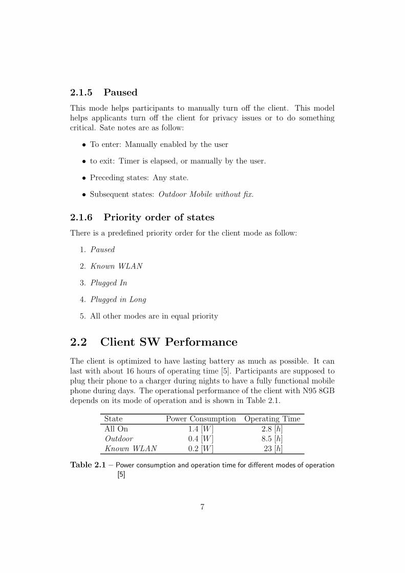
The client is optimized to have lasting battery as much as possible. It canlast with about 16 hours of operating time [5]. Participants are supposed toplug their phone to a charger during nights to have a fully functional mobilephone during days. The operational performance of the client with N95 8GBdepends on its mode of operation and is shown in Table 2.1.
State Power Consumption Operating TimeAll On 1.4 [W ] 2.8 [h]Outdoor 0.4 [W ] 8.5 [h]Known WLAN 0.2 [W ] 23 [h]
Table 2.1 – Power consumption and operation time for different modes of operation[5]
7
2.3 Types of Collected Data
The collected data are listed as follow:
• Localization data like: GPS coordinates, WLAN information and Celltowers details.
• Social data information like: Address book, SMS, BT2 details, and calllogs.
• Media information as pictures, and videos.
• Application usage.
• Control data like: current active profile, Battery level, Ring type andetc.
2.4 Participants
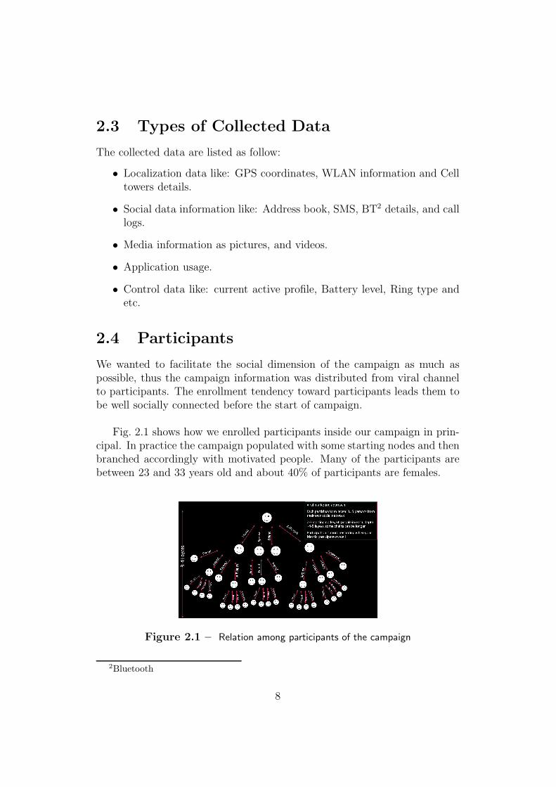
We wanted to facilitate the social dimension of the campaign as much aspossible, thus the campaign information was distributed from viral channelto participants. The enrollment tendency toward participants leads them tobe well socially connected before the start of campaign.
Fig. 2.1 shows how we enrolled participants inside our campaign in prin-cipal. In practice the campaign populated with some starting nodes and thenbranched accordingly with motivated people. Many of the participants arebetween 23 and 33 years old and about 40% of participants are females.
Figure 2.1 – Relation among participants of the campaign
2Bluetooth
8
Chapter 3
Location Estimation
As we discussed previously location based services are emerging mobile ap-plication, but the lack of well covered and accurate positing method havemade a difficult cycle for these kind of user applications. In addition, usersalways wish to have a precise estimation of their location in order to monitorthe places that themselves or their children have been visited. With emerg-ing smart phones market it seems needly to step forward and consider oldlocation estimation methods again. We all know that new mobile phonesare well equipped with different types of sensors for different usage that canalso give us valuable information sources to improve having more meticulousestimation of the users locations.
In the previous chapter we elucidated about campaign client state ma-chine and we said, for example, in Known WLAN state even thought themobile phone could have received GPS signal, it would turn off its GPS re-ceiver. As a result it will lose its track. Thus we need a model for GPS pointsto be able to fill the gaps based on neighbor GPS data. On the other hand,we know that GPS is not accurate and it has errors.
In this chapter we aim to describe GPS and some of its error sources.We also explain the probability distribution that seems to be well describingthese source of errors. We use this distribution model to estimate the posi-tion of the users between times that we have GPS position to fill the missingGPS points. Moreover, we will extend a technique for cases that we do nothave any GPS signals and we lean on other capability of our smart phones.
All the simulations and schemes are based on real data that we collectfrom our participants of the campaign. In this way, we are quite sure thatthe suggested method will be useful for future mobile phone applications.
9
This chapter is started with Global Positioning System and its errorsources then we describe the probability model that we found for each GPSpoint. Furthermore, we will speak about cell towers and their usage in local-ization which is followed by strong potential of WLANs in location estimationand how to approximate the position of WLANs. We utilize all the sourcesof information to have a more reliable location estimation algorithm.
3.1 Global Positioning System
Global positioning system consists of 24 to 32 satellites in Medium EarthOrbit1 and developed by the United States Department of Defense (DoD).
This Satellite positioning method is independent of weather condition andtime and also it is accessible both inshore and offshore. These distinguishedfeatures resulted in its densely usage for military purposes at its time of in-vent, and later it used for civilian 3D positioning and scientific applications.Nowadays, GPS has two frame works one for civil, Standard PositioningService (SPS), and the other for military users, Precise Positioning Service(PPS), the main difference of these two services is their different accuracy [2].
In this section we will shortly review how GPS positing works and itserror sources. Then we explain the probability distribution model of eachGPS point.
3.1.1 Positioning Method
A GPS receiver works with messages from at least 4 visible satellites. It candetermine the time and its corresponding satellite position at the time thata message is sent. The satellite position and the message transmission timefor satellite i is [xi, yi, zi, ti]. If the message is received at tr, then the GPSreceiver can calculate the transmission time as (tr − ti). The distance thatthe message is traveled is calculated by pi = (tr− ti)c in which c is the speedof light.
A satellite position and its distance form the GPS receiver makes a spher-ical surface with the satellite positioned at the center. The GPS receiver
1A region around the Earth with altitude of 1200 miles [4].
10
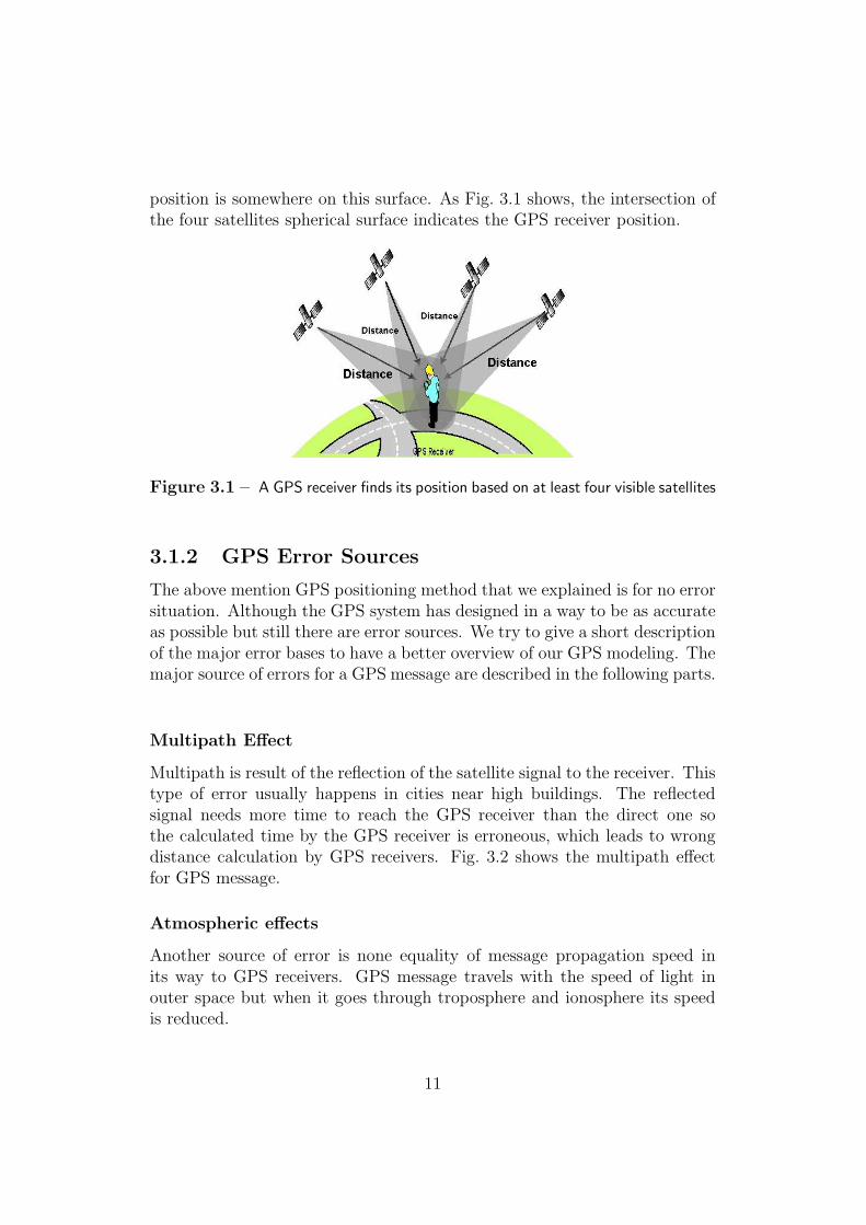
position is somewhere on this surface. As Fig. 3.1 shows, the intersection ofthe four satellites spherical surface indicates the GPS receiver position.
Figure 3.1 – A GPS receiver finds its position based on at least four visible satellites
3.1.2 GPS Error Sources
The above mention GPS positioning method that we explained is for no errorsituation. Although the GPS system has designed in a way to be as accurateas possible but still there are error sources. We try to give a short descriptionof the major error bases to have a better overview of our GPS modeling. Themajor source of errors for a GPS message are described in the following parts.
Multipath Effect
Multipath is result of the reflection of the satellite signal to the receiver. Thistype of error usually happens in cities near high buildings. The reflectedsignal needs more time to reach the GPS receiver than the direct one sothe calculated time by the GPS receiver is erroneous, which leads to wrongdistance calculation by GPS receivers. Fig. 3.2 shows the multipath effectfor GPS message.
Atmospheric effects
Another source of error is none equality of message propagation speed inits way to GPS receivers. GPS message travels with the speed of light inouter space but when it goes through troposphere and ionosphere its speedis reduced.
11
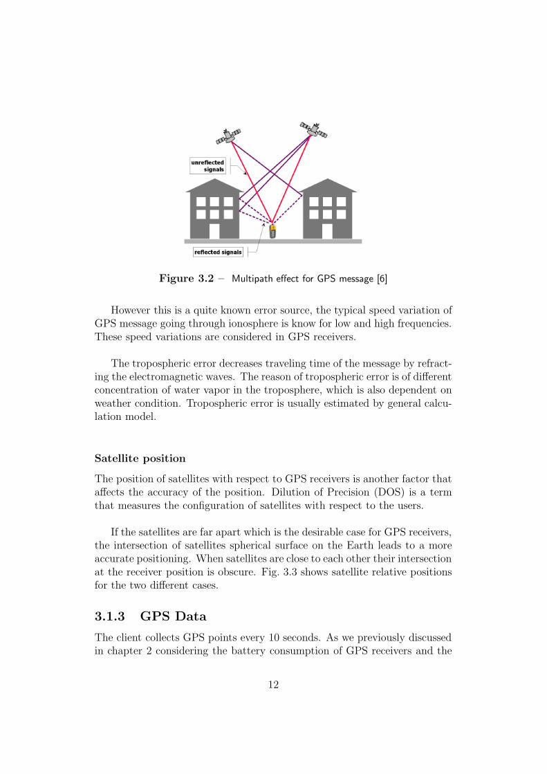
Figure 3.2 – Multipath effect for GPS message [6]
However this is a quite known error source, the typical speed variation ofGPS message going through ionosphere is know for low and high frequencies.These speed variations are considered in GPS receivers.
The tropospheric error decreases traveling time of the message by refract-ing the electromagnetic waves. The reason of tropospheric error is of differentconcentration of water vapor in the troposphere, which is also dependent onweather condition. Tropospheric error is usually estimated by general calcu-lation model.
Satellite position
The position of satellites with respect to GPS receivers is another factor thataffects the accuracy of the position. Dilution of Precision (DOS) is a termthat measures the configuration of satellites with respect to the users.
If the satellites are far apart which is the desirable case for GPS receivers,the intersection of satellites spherical surface on the Earth leads to a moreaccurate positioning. When satellites are close to each other their intersectionat the receiver position is obscure. Fig. 3.3 shows satellite relative positionsfor the two different cases.
3.1.3 GPS Data
The client collects GPS points every 10 seconds. As we previously discussedin chapter 2 considering the battery consumption of GPS receivers and the
12
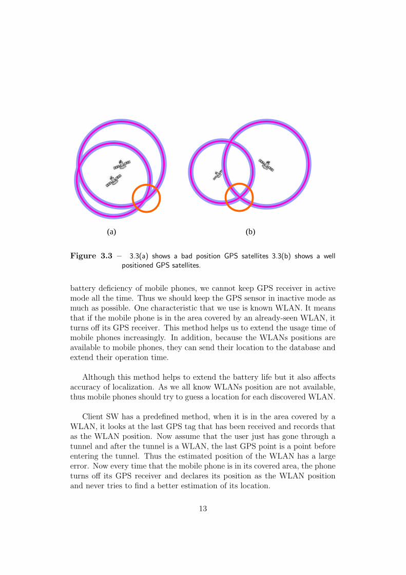
(b)(a)
Figure 3.3 – 3.3(a) shows a bad position GPS satellites 3.3(b) shows a wellpositioned GPS satellites.
battery deficiency of mobile phones, we cannot keep GPS receiver in activemode all the time. Thus we should keep the GPS sensor in inactive mode asmuch as possible. One characteristic that we use is known WLAN. It meansthat if the mobile phone is in the area covered by an already-seen WLAN, itturns off its GPS receiver. This method helps us to extend the usage time ofmobile phones increasingly. In addition, because the WLANs positions areavailable to mobile phones, they can send their location to the database andextend their operation time.
Although this method helps to extend the battery life but it also affectsaccuracy of localization. As we all know WLANs position are not available,thus mobile phones should try to guess a location for each discovered WLAN.
Client SW has a predefined method, when it is in the area covered by aWLAN, it looks at the last GPS tag that has been received and records thatas the WLAN position. Now assume that the user just has gone through atunnel and after the tunnel is a WLAN, the last GPS point is a point beforeentering the tunnel. Thus the estimated position of the WLAN has a largeerror. Now every time that the mobile phone is in its covered area, the phoneturns off its GPS receiver and declares its position as the WLAN positionand never tries to find a better estimation of its location.
13
Whenever the GPS receiver is active, it sends the user location and speedevery 10 seconds. The location is always available but sometimes GPS re-ceiver cannot find the speed so it will not send it.
3.1.4 GPS Error Variance
As we explained, there are many sources of error for a GPS message. In orderto model the error distribution of a GPS point, we need to have the varianceof the error. We tried to have an experiment to collect GPS records duringa time and based on the collected data, we would try to find a distributionmodel for GPS error.
In our experiment we arbitrarily chose a N95 Nokia mobile phone, andput it in the office near a closed window. We tried to locate the position ofthe mobile phone with Google Map, unfortunately, the map was not accu-rate enough so, we could not locate the position of the mobile phone with theGoogle Map. As the result, The average of all collected data would be thebest estimated position of the phone and the error variance was measuredwith respect to this point.
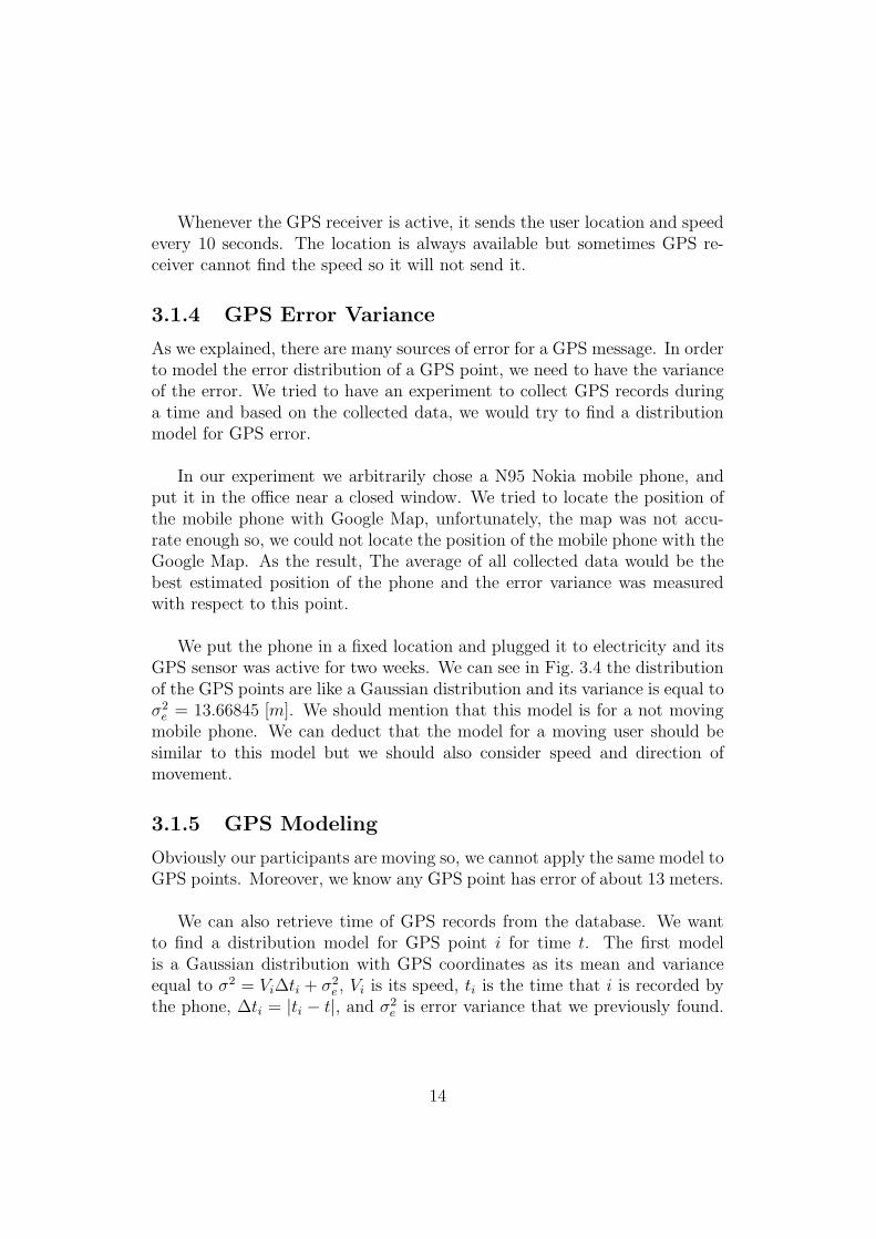
We put the phone in a fixed location and plugged it to electricity and itsGPS sensor was active for two weeks. We can see in Fig. 3.4 the distributionof the GPS points are like a Gaussian distribution and its variance is equal toσ2
e = 13.66845 [m]. We should mention that this model is for a not movingmobile phone. We can deduct that the model for a moving user should besimilar to this model but we should also consider speed and direction ofmovement.
3.1.5 GPS Modeling
Obviously our participants are moving so, we cannot apply the same model toGPS points. Moreover, we know any GPS point has error of about 13 meters.
We can also retrieve time of GPS records from the database. We wantto find a distribution model for GPS point i for time t. The first modelis a Gaussian distribution with GPS coordinates as its mean and varianceequal to σ2 = Vi∆ti + σ2
e , Vi is its speed, ti is the time that i is recorded bythe phone, ∆ti = |ti − t|, and σ2
e is error variance that we previously found.
14
0 5 10 15 20 25 300
5
10
15
20
25
30
35
40
45
50
Latitude [m]
Long
itude
[m]
Sampled GPS of a N95 for a Location during 2 Weeks
GPS PositionActual Position
Figure 3.4 – Sample of N95 GPS sensor output for a specific position during 2weeks.
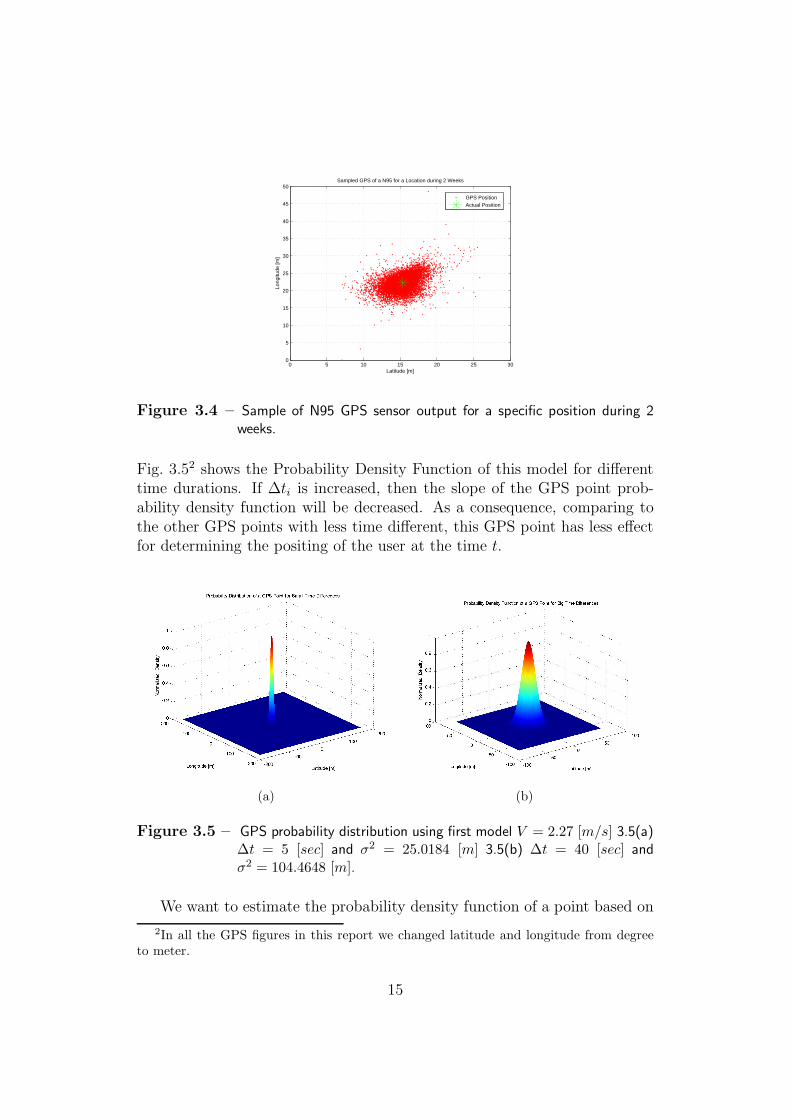
Fig. 3.52 shows the Probability Density Function of this model for differenttime durations. If ∆ti is increased, then the slope of the GPS point prob-ability density function will be decreased. As a consequence, comparing tothe other GPS points with less time different, this GPS point has less effectfor determining the positing of the user at the time t.
(a) (b)
Figure 3.5 – GPS probability distribution using first model V = 2.27 [m/s] 3.5(a)∆t = 5 [sec] and σ2 = 25.0184 [m] 3.5(b) ∆t = 40 [sec] andσ2 = 104.4648 [m].
We want to estimate the probability density function of a point based on
2In all the GPS figures in this report we changed latitude and longitude from degreeto meter.
15
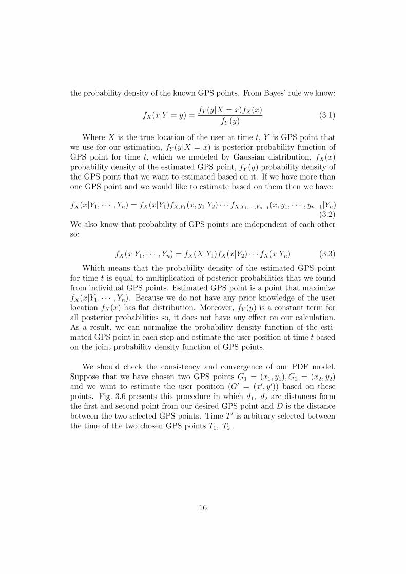
the probability density of the known GPS points. From Bayes’ rule we know:
fX(x|Y = y) =fY (y|X = x)fX(x)
fY (y)(3.1)
Where X is the true location of the user at time t, Y is GPS point thatwe use for our estimation, fY (y|X = x) is posterior probability function ofGPS point for time t, which we modeled by Gaussian distribution, fX(x)probability density of the estimated GPS point, fY (y) probability density ofthe GPS point that we want to estimated based on it. If we have more thanone GPS point and we would like to estimate based on them then we have:
fX(x|Y1, · · · , Yn) = fX(x|Y1)fX,Y1(x, y1|Y2) · · · fX,Y1,··· ,Yn−1
(x, y1, · · · , yn−1|Yn)(3.2)
We also know that probability of GPS points are independent of each otherso:
fX(x|Y1, · · · , Yn) = fX(X|Y1)fX(x|Y2) · · ·fX(x|Yn) (3.3)
Which means that the probability density of the estimated GPS pointfor time t is equal to multiplication of posterior probabilities that we foundfrom individual GPS points. Estimated GPS point is a point that maximizefX(x|Y1, · · · , Yn). Because we do not have any prior knowledge of the userlocation fX(x) has flat distribution. Moreover, fY (y) is a constant term forall posterior probabilities so, it does not have any effect on our calculation.As a result, we can normalize the probability density function of the esti-mated GPS point in each step and estimate the user position at time t basedon the joint probability density function of GPS points.
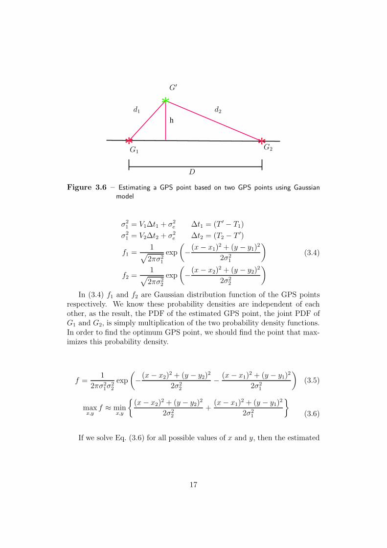
We should check the consistency and convergence of our PDF model.Suppose that we have chosen two GPS points G1 = (x1, y1), G2 = (x2, y2)and we want to estimate the user position (G′ = (x′, y′)) based on thesepoints. Fig. 3.6 presents this procedure in which d1, d2 are distances formthe first and second point from our desired GPS point and D is the distancebetween the two selected GPS points. Time T ′ is arbitrary selected betweenthe time of the two chosen GPS points T1, T2.
16
* *G1G2
G′
d1 d2
h
*
D
Figure 3.6 – Estimating a GPS point based on two GPS points using Gaussianmodel
σ21 = V1∆t1 + σ2
e ∆t1 = (T ′ − T1)
σ21 = V2∆t2 + σ2
e ∆t2 = (T2 − T ′)
f1 =1√2πσ2
1
exp
(−(x− x1)
2 + (y − y1)2
2σ21
)
f2 =1√2πσ2
2
exp
(−(x− x2)
2 + (y − y2)2
2σ22
)(3.4)
In (3.4) f1 and f2 are Gaussian distribution function of the GPS pointsrespectively. We know these probability densities are independent of eachother, as the result, the PDF of the estimated GPS point, the joint PDF ofG1 and G2, is simply multiplication of the two probability density functions.In order to find the optimum GPS point, we should find the point that max-imizes this probability density.
f =1
2πσ21σ
22
exp
(−(x− x2)
2 + (y − y2)2
2σ22
− (x− x1)2 + (y − y1)
2
2σ21
)(3.5)
maxx,y
f ≈ minx,y
{(x− x2)
2 + (y − y2)2
2σ22
+(x− x1)
2 + (y − y1)2
2σ21
}
(3.6)
If we solve Eq. (3.6) for all possible values of x and y, then the estimated
17
GPS point is as follows:
x′ =x2 + Kx1
1 + Kwhere K =
σ21
σ21
y′ =y2 + Ky1
1 + K
(3.7)
If we have estimation based on n GPS points, by induction the coordi-nates are as follow:
x′ =
n∑
i=1
xi
σ2i
n∑
i=1
1
σ2i
y′ =
n∑
i=1
yi
σ2i
n∑
i=1
1
σ2i
(3.8)
To check the convergence of the model, we will use a simple example.We try to guess a GPS position for a given time based on infinite numberof GPS points having the following characteristics; their speed are the sameand equal to Vi = 1 [m/s] and they are positioned on a line with 1 meterdistance from each other. We proved in Eq. (3.8) that x′ =
∑∞
i=1xi
σ2
i
/∑
∞
i=11σ2
i
and σ2i = |i− t′|+σ2
e . In addition, by using integral test theorem3 from seriesconvergence methods, we can deduct that
∑∞
i=1xi
σ2
i
, is a divergent series, thus
this model is not an appropriate model for our problem.
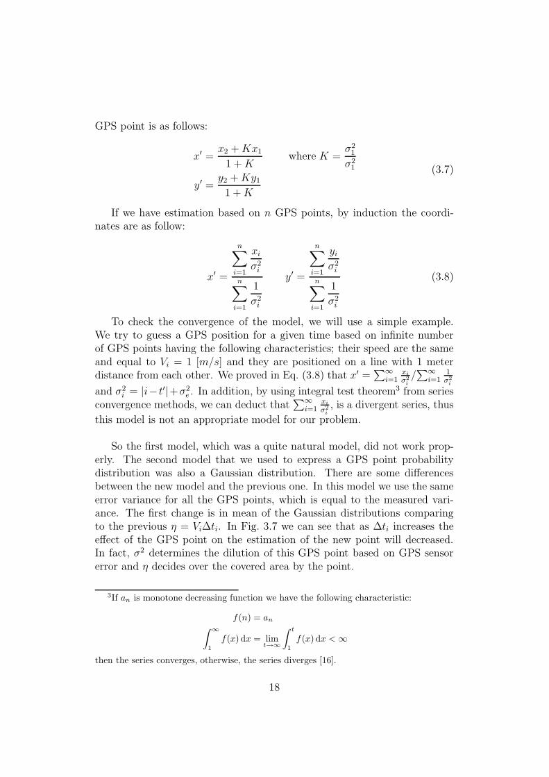
So the first model, which was a quite natural model, did not work prop-erly. The second model that we used to express a GPS point probabilitydistribution was also a Gaussian distribution. There are some differencesbetween the new model and the previous one. In this model we use the sameerror variance for all the GPS points, which is equal to the measured vari-ance. The first change is in mean of the Gaussian distributions comparingto the previous η = Vi∆ti. In Fig. 3.7 we can see that as ∆ti increases theeffect of the GPS point on the estimation of the new point will decreased.In fact, σ2 determines the dilution of this GPS point based on GPS sensorerror and η decides over the covered area by the point.
3If an is monotone decreasing function we have the following characteristic:
f(n) = an
∫∞
1
f(x) dx = limt→∞
∫t
1
f(x) dx <∞
then the series converges, otherwise, the series diverges [16].
18
(a) (b)
Figure 3.7 – GPS probability distribution for different time durations σ2 =13.66845 [m] 3.7(a) ∆ti = 5 [sec] and η = 1.2 [m] Recording time ofthis GPS point is near the selected time 3.7(b) ∆ti = 105 [sec] andη = 149.612 [m]. We can see as ∆ti increases the effect of the GPSpoint will be decreased.
We can see that in this model every direction around GPS point has thesame worth and its probability value will be decreased, as we go farther awayfrom the GPS point. So all the points on a circle around the GPS point hasthe same probability value. On the other hand, we know that when you takea path and follow it toward your destination, all the points aligned with yourdirection are more probable comparing to other points on the same circle buton a wrong direction.
Fig. 3.7 shows that this restriction has not taken into account in ourmodel. So we should improve our model. To find a direction for each GPSpoint, we will take into account the effect of the previous and the next GPSpoints. Assume that you want to go from your home to your office and youhave chosen your way to your office and started your GPS receiver. Eachrecorded GPS point is in your path toward your destination and also affectedby your previous position and has influence on your next points.
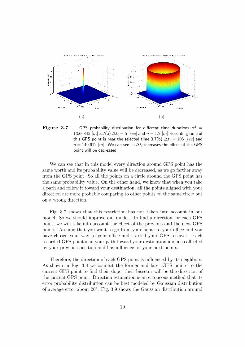
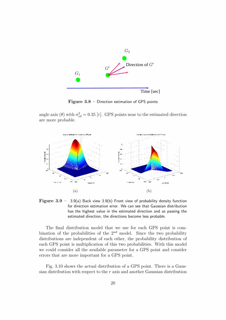
Therefore, the direction of each GPS point is influenced by its neighbors.As shown in Fig. 3.8 we connect the former and later GPS points to thecurrent GPS point to find their slope, their bisector will be the direction ofthe current GPS point. Direction estimation is an erroneous method that itserror probability distribution can be best modeled by Gaussian distributionof average error about 20◦. Fig. 3.9 shows the Gaussian distribution around
19
bb
b
G1
G′
G2
Direction of G′
Time [sec]
Figure 3.8 – Direction estimation of GPS points
angle axis (θ) with σ2ed = 0.35 [r]. GPS points near to the estimated direction
are more probable.
(a) (b)
Figure 3.9 – 3.9(a) Back view 3.9(b) Front view of probability density functionfor direction estimation error. We can see that Gaussian distributionhas the highest value in the estimated direction and as passing theestimated direction, the directions become less probable.
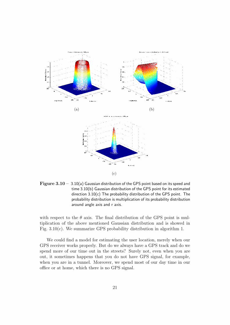
The final distribution model that we use for each GPS point is com-bination of the probabilities of the 2nd model. Since the two probabilitydistributions are independent of each other, the probability distribution ofeach GPS point is multiplication of this two probabilities. With this modelwe could consider all the available parameter for a GPS point and considererrors that are more important for a GPS point.
Fig. 3.10 shows the actual distribution of a GPS point. There is a Gaus-sian distribution with respect to the r axis and another Gaussian distribution
20
(a) (b)
(c)
Figure 3.10 – 3.10(a) Gaussian distribution of the GPS point based on its speed andtime 3.10(b) Gaussian distribution of the GPS point for its estimateddirection 3.10(c) The probability distribution of the GPS point. Theprobability distribution is multiplication of its probability distributionaround angle axis and r axis.
with respect to the θ axis. The final distribution of the GPS point is mul-tiplication of the above mentioned Gaussian distribution and is showed inFig. 3.10(c). We summarize GPS probability distribution in algorithm 1.
We could find a model for estimating the user location, merely when ourGPS receiver works properly. But do we always have a GPS track and do wespend more of our time out in the streets? Surely not, even when you areout, it sometimes happens that you do not have GPS signal, for example,when you are in a tunnel. Moreover, we spend most of our day time in ouroffice or at home, which there is no GPS signal.
21
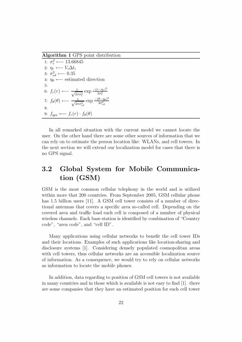
Algorithm 1 GPS point distribution
1: σ2e ←− 13.66845
2: ηr ←− Vi∆ti3: σ2
ed ←− 0.354: ηθ ←− estimated direction5:
6: fr(r)←− 1√2πσ2
e
exp −(r−ηr)2
2σ2e
7: fθ(θ)←− 1√2πσ2
ed
exp −(θ−ηθ)2
2σ2
ed
8:
9: fgps ←− fr(r) · fθ(θ)
In all remarked situation with the current model we cannot locate theuser. On the other hand there are some other sources of information that wecan rely on to estimate the person location like: WLANs, and cell towers. Inthe next section we will extend our localization model for cases that there isno GPS signal.
3.2 Global System for Mobile Communica-
tion (GSM)
GSM is the most common cellular telephony in the world and is utilizedwithin more that 200 countries. From September 2005, GSM cellular phonehas 1.5 billion users [11]. A GSM cell tower consists of a number of direc-tional antennas that covers a specific area so-called cell. Depending on thecovered area and traffic load each cell is composed of a number of physicalwireless channels. Each base station is identified by combination of “Countrycode”, “area code”, and “cell ID”.
Many applications using cellular networks to benefit the cell tower IDsand their locations. Examples of such applications like location-sharing anddisclosure systems [1]. Considering densely populated cosmopolitan areaswith cell towers, thus cellular networks are an accessible localization sourceof information. As a consequence, we would try to rely on cellular networksas information to locate the mobile phones.
In addition, data regarding to position of GSM cell towers is not availablein many countries and in those which is available is not easy to find [1]. thereare some companies that they have an estimated position for each cell tower
22
for their internal usage. Fortunately, we could find a location for most ofthe cell tower seen in our campaign from one of this companies4. Physicallocation of GSM cell towers helps us to have an estimation of the mobilelocation.
3.2.1 Localization Using GSM Cell Towers
In each stamp of time a mobile phone is connected to a GSM cell tower, be-side that there are usually other cell towers that could also cover the phone.If the mobile phone could record all the cell towers that it can see, by havingthe range and position of the cell towers, then we could locate the mobilephone. If we assume that the mobile phone could pick three or more celltowers, we can compute its approximate location in relation to these celltowers.
Our campaign software is just able to find the cell tower ID that the mo-bile is connected, and cannot discover other cell towers that are in range. Onthe other hand, GSM cell towers usually cover a large area so, localizationbased on a GSM cell towers cannot be accurate.
Although GSM cell towers are a source of information that is alwaysavailable, we just use it in crucial situations that we do not have any othersource of information except the GSM cell tower ID that the mobile phoneis connected. Mostly, WLANs are more reliable for user positioning.
3.2.2 GSM Cell Tower Application
An interesting usage of GSM cell towers is to find places that the user spendsmost of his time during a day, like office, and home. When we are in a placefor a long duration of time, the cell tower ID will remain permanent. In theother hand, during this period we do not change out GSM cell tower. Thus,if we look at cell towers that are seen by a mobile phone, there are somecell towers that the user has spent considerably longer time connecting withthem comparing to other cell towers. Those cell towers are ones that coverthe places that the user spends most of his time.
Another application of GSM towers can be movement detection. Wealready said if users do not move, they are connected to a certain cell toweras they start moving the cell towers that they are connecting begins to change.
4The company that we used to find location of cell towers is: Open Cellid
23
By deciding over a time that we can consider the user in standing position,we would be able to detect the movement of participants [8].
3.3 Wireless LANs
Wireless LANs (WLAN) were built to give the possibility to access a fixednetwork architectures. Because of their flexibility, connectivity and their lowprice, their market is growing rapidly. A group of them are classified withIEEE 802.11 working group and amongst 802.11b has become the most suc-cessful one. They work up to 11 Mbps and operate in 2.4 GHz band whichis the ISM band5 [7].
3.3.1 Indoor Positioning
GPS is the main positioning system; however, it does not work in indoorplaces. Knowing the position of a user is of great importance, for this reasonthere are some systems that are specifically built for indoor positioning suchas Active Badge, Cricket, and the Bat that can be used for indoor positioning[11].
These systems are costly and not everybody can utilize them. Some ex-isting infrastructures that can be used are like television signals and WirelessLANs [10]. WLAN positioning is the easiest among those methods [7].
3.3.2 Wireless LAN Positioning
As we previously mentioned GPS is not available in indoor places and duringthis time we can make profit from WLANs or cell towers information as asource of information to locate the mobile user. In addition, we know GSMcell towers are not an accurate source of information for position estimation.
The only problem for WLAN positioning is that we do not know theposition of WLANs. If we could somehow find their position then we wouldbe able to utilize them to find the user location. Thus we firstly explain themethod that we use to find the WLANs’ position then we will describe howwe use their position to estimate the position of the user.
5industrial, scientific and medical (ISM) radio bands
24
Ascertaining WLANs Position
The client SW has the possibility to search for all WLANs every 60 secondsand records their MAC address. Now assume that at the time that our mo-bile phone sees a WLAN it also has GPS signal so, it can impute the GPSposition (PGPS) of the WLAN. On the other hand, the mobile phone is notexactly at the position of Access Point (AP), so there is an error of about50 meters for estimating of the WLANs position (PAP ) depending on thecovering range of WLAN. To decrease this error we would check the GPSevery time that the mobile phone is in the range of that WLAN and takethe average position as the position of that WLAN. Moreover, consideringnumber of participants in our campaign, we are supposed to have a goodestimation for popular6 WLANs.
The challenging issue is the indoor WLANs. For this type of WLANs,we do not have GPS signal at their AP location. Only for a small portionof these WLANs, when the mobile phone is covered by them, the phone canreceive GPS signal.
The method that we use for positioning of this series is as follows: whena mobile phone is in range of a WLAN from this kind, it will look at the last50 second of its GPS track. We assumed that a person cannot go too far in50 seconds.
If there is any GPS position available, it will take the one with leasttime difference, between the time that the GPS point is recorded and thatof WLAN search, as the WLAN position. We iterate this method for eachWLAN in every time that they are seen. At last we take the average of theall estimation as of the WLAN position. We summarize WLAN positioningin the algorithm 2.
3.4 Position Estimation
Our position estimation method consists of two separate modes based onavailability of GPS signal:
1. GPS Mode
2. WLAN-GSM Mode
6WLANs that are seen with many participants of the campaign.
25
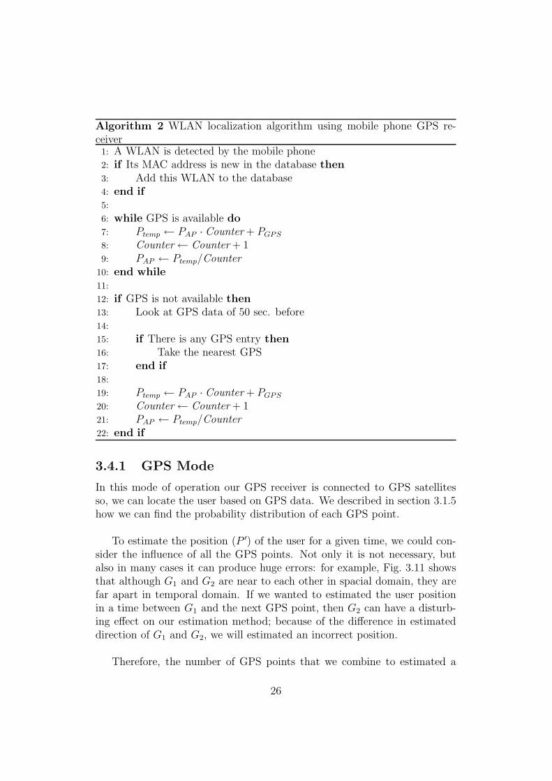
Algorithm 2 WLAN localization algorithm using mobile phone GPS re-ceiver1: A WLAN is detected by the mobile phone2: if Its MAC address is new in the database then3: Add this WLAN to the database4: end if5:
6: while GPS is available do7: Ptemp ← PAP · Counter + PGPS
8: Counter← Counter + 19: PAP ← Ptemp/Counter
10: end while11:
12: if GPS is not available then13: Look at GPS data of 50 sec. before14:
15: if There is any GPS entry then16: Take the nearest GPS17: end if18:
19: Ptemp ← PAP · Counter + PGPS
20: Counter← Counter + 121: PAP ← Ptemp/Counter
22: end if
3.4.1 GPS Mode
In this mode of operation our GPS receiver is connected to GPS satellitesso, we can locate the user based on GPS data. We described in section 3.1.5how we can find the probability distribution of each GPS point.
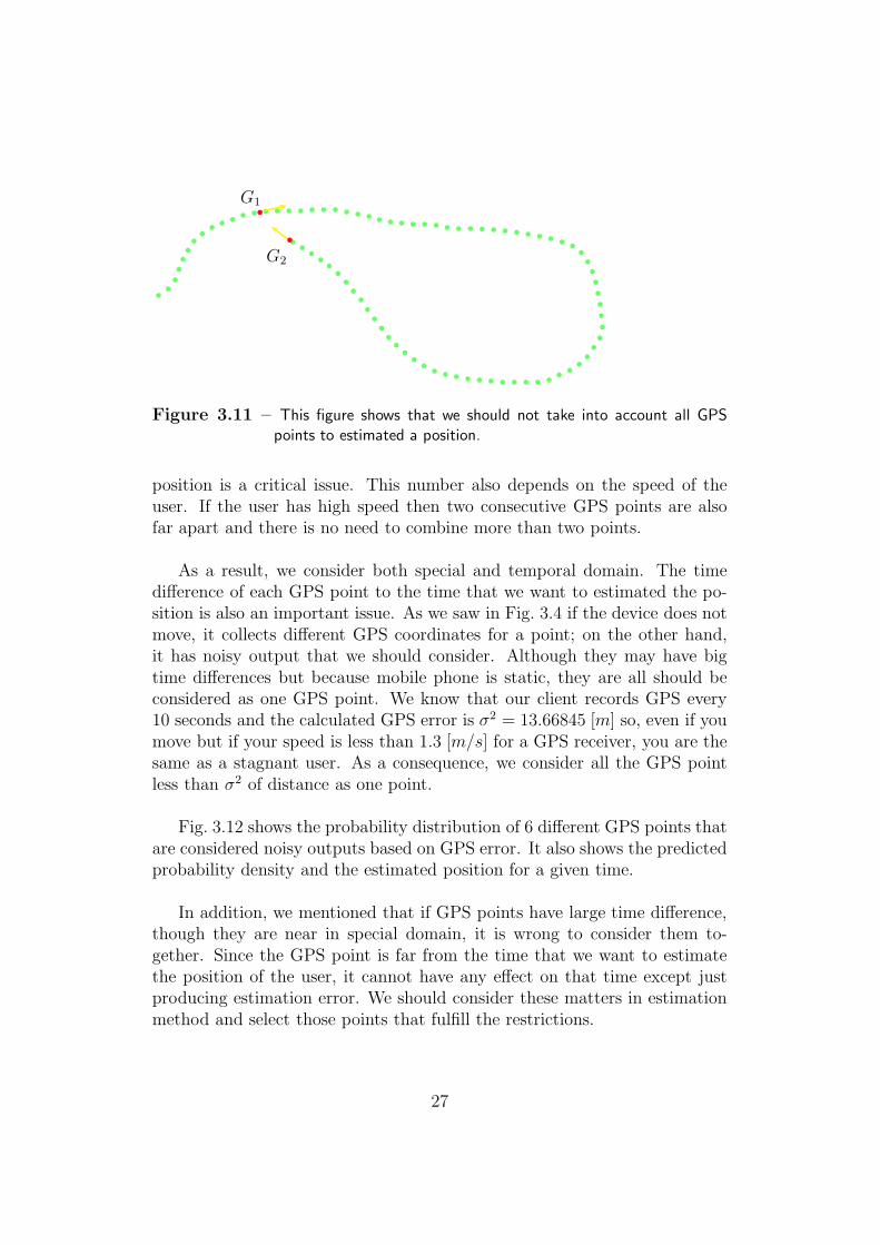
To estimate the position (P ′) of the user for a given time, we could con-sider the influence of all the GPS points. Not only it is not necessary, butalso in many cases it can produce huge errors: for example, Fig. 3.11 showsthat although G1 and G2 are near to each other in spacial domain, they arefar apart in temporal domain. If we wanted to estimated the user positionin a time between G1 and the next GPS point, then G2 can have a disturb-ing effect on our estimation method; because of the difference in estimateddirection of G1 and G2, we will estimated an incorrect position.
Therefore, the number of GPS points that we combine to estimated a
26
G1
G2
b
b
Figure 3.11 – This figure shows that we should not take into account all GPSpoints to estimated a position.
position is a critical issue. This number also depends on the speed of theuser. If the user has high speed then two consecutive GPS points are alsofar apart and there is no need to combine more than two points.
As a result, we consider both special and temporal domain. The timedifference of each GPS point to the time that we want to estimated the po-sition is also an important issue. As we saw in Fig. 3.4 if the device does notmove, it collects different GPS coordinates for a point; on the other hand,it has noisy output that we should consider. Although they may have bigtime differences but because mobile phone is static, they are all should beconsidered as one GPS point. We know that our client records GPS every10 seconds and the calculated GPS error is σ2 = 13.66845 [m] so, even if youmove but if your speed is less than 1.3 [m/s] for a GPS receiver, you are thesame as a stagnant user. As a consequence, we consider all the GPS pointless than σ2 of distance as one point.
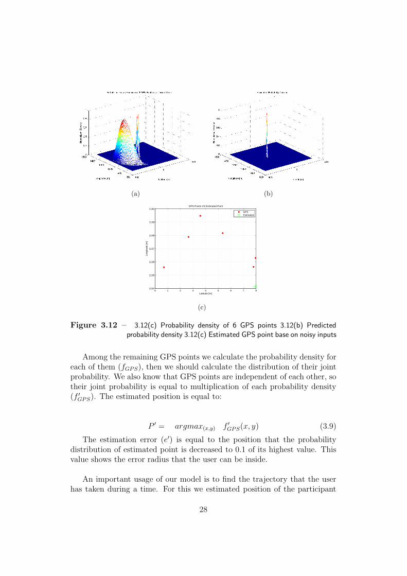
Fig. 3.12 shows the probability distribution of 6 different GPS points thatare considered noisy outputs based on GPS error. It also shows the predictedprobability density and the estimated position for a given time.
In addition, we mentioned that if GPS points have large time difference,though they are near in special domain, it is wrong to consider them to-gether. Since the GPS point is far from the time that we want to estimatethe position of the user, it cannot have any effect on that time except justproducing estimation error. We should consider these matters in estimationmethod and select those points that fulfill the restrictions.
27
(a) (b)
0 1 2 3 4 5 6 7 81134
1135
1136
1137
1138
1139
1140
Latitude [m]
Long
itude
[m]
GPS Points VS Estimated Point
GPSEstimated
(c)
Figure 3.12 – 3.12(c) Probability density of 6 GPS points 3.12(b) Predictedprobability density 3.12(c) Estimated GPS point base on noisy inputs
Among the remaining GPS points we calculate the probability density foreach of them (fGPS), then we should calculate the distribution of their jointprobability. We also know that GPS points are independent of each other, sotheir joint probability is equal to multiplication of each probability density(f ′
GPS). The estimated position is equal to:
P ′ = argmax(x,y) f ′
GPS(x, y) (3.9)
The estimation error (e′) is equal to the position that the probabilitydistribution of estimated point is decreased to 0.1 of its highest value. Thisvalue shows the error radius that the user can be inside.
An important usage of our model is to find the trajectory that the userhas taken during a time. For this we estimated position of the participant
28
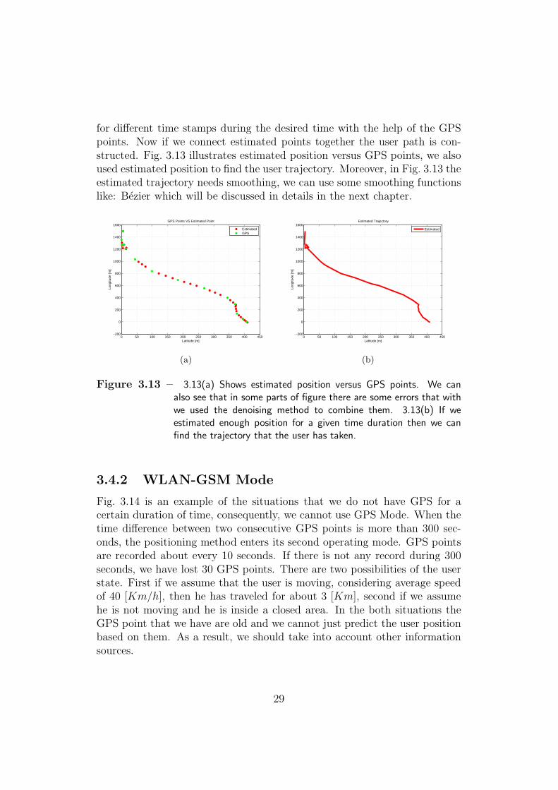
for different time stamps during the desired time with the help of the GPSpoints. Now if we connect estimated points together the user path is con-structed. Fig. 3.13 illustrates estimated position versus GPS points, we alsoused estimated position to find the user trajectory. Moreover, in Fig. 3.13 theestimated trajectory needs smoothing, we can use some smoothing functionslike: Bezier which will be discussed in details in the next chapter.
0 50 100 150 200 250 300 350 400 450−200
0
200
400
600
800
1000
1200
1400
1600
Long
itude
[m]
Latitude [m]
GPS Points VS Estimated Point
EstimatedGPS
(a)
0 50 100 150 200 250 300 350 400 450−200
0
200
400
600
800
1000
1200
1400
1600
Long
itude
[m]
Estimated Trajectory
Latitude [m]
Estimated
(b)
Figure 3.13 – 3.13(a) Shows estimated position versus GPS points. We canalso see that in some parts of figure there are some errors that withwe used the denoising method to combine them. 3.13(b) If weestimated enough position for a given time duration then we canfind the trajectory that the user has taken.
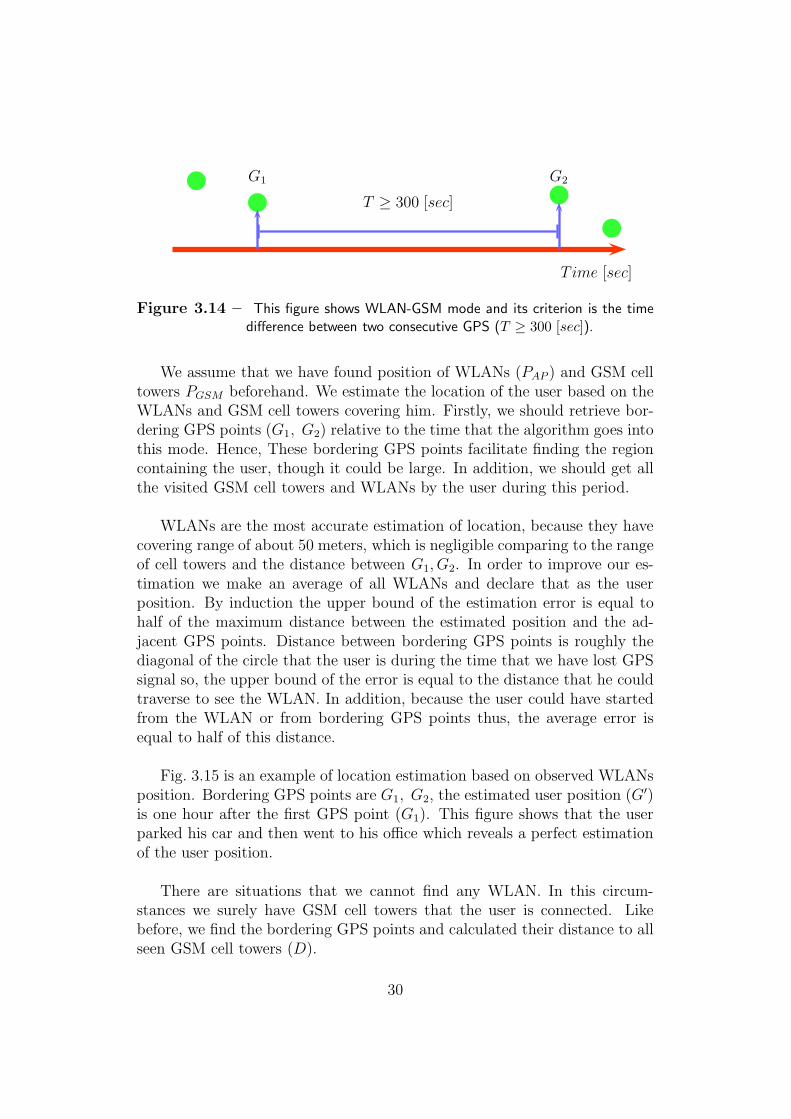
3.4.2 WLAN-GSM Mode
Fig. 3.14 is an example of the situations that we do not have GPS for acertain duration of time, consequently, we cannot use GPS Mode. When thetime difference between two consecutive GPS points is more than 300 sec-onds, the positioning method enters its second operating mode. GPS pointsare recorded about every 10 seconds. If there is not any record during 300seconds, we have lost 30 GPS points. There are two possibilities of the userstate. First if we assume that the user is moving, considering average speedof 40 [Km/h], then he has traveled for about 3 [Km], second if we assumehe is not moving and he is inside a closed area. In the both situations theGPS point that we have are old and we cannot just predict the user positionbased on them. As a result, we should take into account other informationsources.
29
bb
bb
T ime [sec]
T ≥ 300 [sec]
G1 G2
Figure 3.14 – This figure shows WLAN-GSM mode and its criterion is the timedifference between two consecutive GPS (T ≥ 300 [sec]).
We assume that we have found position of WLANs (PAP ) and GSM celltowers PGSM beforehand. We estimate the location of the user based on theWLANs and GSM cell towers covering him. Firstly, we should retrieve bor-dering GPS points (G1, G2) relative to the time that the algorithm goes intothis mode. Hence, These bordering GPS points facilitate finding the regioncontaining the user, though it could be large. In addition, we should get allthe visited GSM cell towers and WLANs by the user during this period.
WLANs are the most accurate estimation of location, because they havecovering range of about 50 meters, which is negligible comparing to the rangeof cell towers and the distance between G1, G2. In order to improve our es-timation we make an average of all WLANs and declare that as the userposition. By induction the upper bound of the estimation error is equal tohalf of the maximum distance between the estimated position and the ad-jacent GPS points. Distance between bordering GPS points is roughly thediagonal of the circle that the user is during the time that we have lost GPSsignal so, the upper bound of the error is equal to the distance that he couldtraverse to see the WLAN. In addition, because the user could have startedfrom the WLAN or from bordering GPS points thus, the average error isequal to half of this distance.
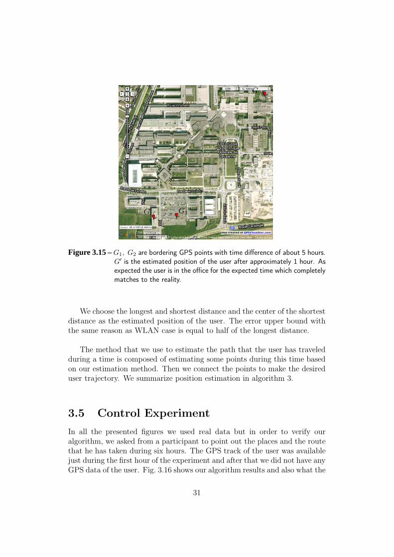
Fig. 3.15 is an example of location estimation based on observed WLANsposition. Bordering GPS points are G1, G2, the estimated user position (G′)is one hour after the first GPS point (G1). This figure shows that the userparked his car and then went to his office which reveals a perfect estimationof the user position.
There are situations that we cannot find any WLAN. In this circum-stances we surely have GSM cell towers that the user is connected. Likebefore, we find the bordering GPS points and calculated their distance to allseen GSM cell towers (D).
30
G2
G1G′
Figure 3.15 –G1, G2 are bordering GPS points with time difference of about 5 hours.
G′ is the estimated position of the user after approximately 1 hour. As
expected the user is in the office for the expected time which completely
matches to the reality.
We choose the longest and shortest distance and the center of the shortestdistance as the estimated position of the user. The error upper bound withthe same reason as WLAN case is equal to half of the longest distance.
The method that we use to estimate the path that the user has traveledduring a time is composed of estimating some points during this time basedon our estimation method. Then we connect the points to make the desireduser trajectory. We summarize position estimation in algorithm 3.
3.5 Control Experiment
In all the presented figures we used real data but in order to verify ouralgorithm, we asked from a participant to point out the places and the routethat he has taken during six hours. The GPS track of the user was availablejust during the first hour of the experiment and after that we did not have anyGPS data of the user. Fig. 3.16 shows our algorithm results and also what the
31
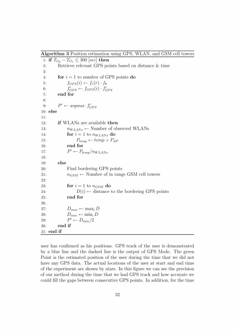
Algorithm 3 Position estimation using GPS, WLAN, and GSM cell towers
1: if TG2− TG1
≤ 300 [sec] then2: Retrieve relevant GPS points based on distance & time3:
4: for i = 1 to number of GPS points do5: fGPS(i)← fr(r) · fθ
6: f ′GPS ← fGPS(i) · f ′
GPS
7: end for8:
9: P ′ ← argmax f ′GPS
10: else11:
12: if WLANs are available then13: nWLANs ← Number of observed WLANs14: for i = 1 to nWLANs do15: Ptemp ← temp + PAP
16: end for17: P ′ ← Ptemp/nWLANs
18:
19: else20: Find bordering GPS points21: nGSM ← Number of in range GSM cell towers22:
23: for i = 1 to nGSM do24: D(i)← distance to the bordering GPS points25: end for26:
27: Dmax ← maxi D28: Dmin ← mini D29: P ′ ← Dmin/230: end if31: end if
user has confirmed as his positions. GPS track of the user is demonstratedby a blue line and the dashed line is the output of GPS Mode. The greenPoint is the estimated position of the user during the time that we did nothave any GPS data. The actual locations of the user at start and end timeof the experiment are shown by stars. In this figure we can see the precisionof our method during the time that we had GPS track and how accurate wecould fill the gaps between consecutive GPS points. In addition, for the time
32
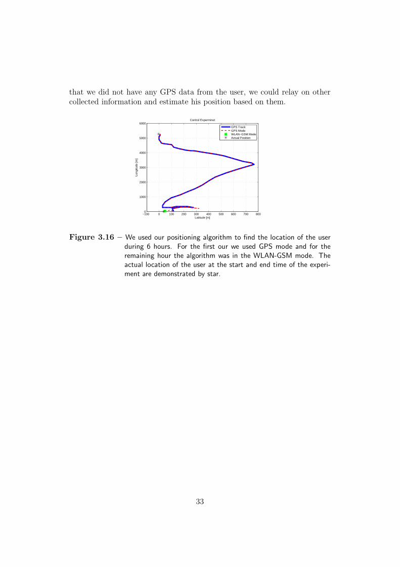
that we did not have any GPS data from the user, we could relay on othercollected information and estimate his position based on them.
−100 0 100 200 300 400 500 600 700 8000
1000
2000
3000
4000
5000
6000
Latitude [m]
Long
itude
[m]
Control Experminet
GPS TrackGPS ModeWLAN−GSM ModeActual Position
Figure 3.16 – We used our positioning algorithm to find the location of the userduring 6 hours. For the first our we used GPS mode and for theremaining hour the algorithm was in the WLAN-GSM mode. Theactual location of the user at the start and end time of the experi-ment are demonstrated by star.
33
Chapter 4
Trajectory Learning and FuturePath Estimation
As we saw in the previous chapter the estimated path needs smoothing so,we will explain some smoothing algorithms and compare their results overGPS trajectories. In addition, We want to predict the most common paththat a user takes; for example, from his home to his office. For the purposewe should find the ROIs 1 of the user, which is possible based on WLANsand GSM cell towers.
Having ROIs and routes that the user takes among his ROIs help us tolearn the most probable paths for his traveling among ROIs. For learningthese routes, we would have many superimposed trajectories that are col-lected during the time that the user participates in the data collection cam-paign. Then we have a set of unorganized data points that we use smoothingalgorithms to find the most common trajectory that the user takes.
In this chapter we will discuss about Bezier curves and their usage insmoothing data points We also discuss two different smoothing algorithmbased on B-spline curves. At last, we will explain future path estimation andthe usage of B-spline smoothing in this area.
4.1 Smoothing
We consider GPS points as a set of unorganized data points2 Xk, k =1, 2, · · ·n, which represents an unknown but not-self intersecting curve that
1Region Of Interest2Because in general users take unpredictable moving direction and speed.
34
we want to compute its approximated curve. Unorganized data points arecalled point cloud and the final approximated curve is called target curve
[13]. Given data points Xk, we want to find target curve P(t) such that theobjective function f is minimized3.
f =n∑
k=1
mint‖P(t)−Xk‖2 + λfs (4.1)
(4.1) means the points of P(t) should have less possible distance to thepoint cloud. fs is regularization factor to assure a smooth output, and λ isa weight constant.
To find a desired target curve, we will introduce two curve fitting methodwhich utilize Bzier curves. Then we will benefit of these curve fitting methodfor smoothing.
4.1.1 Bezier Curve
An important parametric model for smoothing is Bezier curves. Bezier curveswere invented by Pierre Bezier for designing automobile body in 1962 [14].A Bezier curve of degree n is defined as follow:
P(t) =
n∑
i=0
Bi(t)Pi t ∈ [t0, tk]4 (4.2)
In (4.2) Pi is control point such that P (t0) = P0, P (tn) = Pn and Bi(t)is a Bernstein polynomial represented as:
Bi(t) =
(n
k
)( t1 − t
t1 − t0
)n−i( t− t0t1 − t0
)ii ∈ {0, 1, · · · , n} (4.3)
Bezier curves have some special properties that makes them useful forpath planning [14]:
• The curve end points are P0, Pn.
• They are within convex hull of the control points.
3‖x‖ =√
xTx
4For this report we take t0 = 0, tk = 1.
35
Now we defined two curve fitting algorithm that use Bezier curves as theirfitting function which are different in the number of control points.
4.2 Single Control Point Error Minimization
We start with a simple Bezier curve with degree equal to n = 3. We will tryto find a curve fitting method based on quadratic Bezier. Bases of quadraticBezier are B0(t) = (1− t)2, B1(t) = 2t(1− t), and B2(t) = t2. As we men-tioned the point cloud is Xk, k = 1, 2, · · ·n in which x1, and xk are the userROIs, which we want to find the trajectory of the user between them. Theposition of ROIs are know exactly and we want to find the smoothest paththat connects them.
We define P0 as x0 and P2 as xk, which are fixed during all states of prob-lem, now we should choose P1 in a way that we have the smoothest possiblecurve. We propose an algorithm based on iterative error minimization andgradient vector D. We guess an initial value for P1 and iteratively update itby D. Firstly, we propose a way to find a good initial estimation of P1.
4.2.1 Initial Estimation of P1
A good initial estimate of P1 helps us to decrease the number of iterationsso, the algorithm diverge faster if we choose an proper value for P1. For thisreason, we will explain an initial estimation method for P1, which is wellsuited for this method (more details are available in [15]). We consider spaceS spanned by {ϕi}i∈I where I = 1, 2 as follow:
ϕ0 = P0
ϕ1 =P2 −P0
‖P2 −P0‖(4.4)
Each point xi of the point cloud in the space S is represented as [12]:
xi = PS(xi) =∑
j∈I
< ϕj,xi > ϕj (4.5)
Now we consider the projection of xi into subspace S ′ where as follows:
xi = PS′(xi) = ϕ0 + αϕ1 α = ϕT
1 (xi − ϕ0) (4.6)
36
For the initial estimation of P1 we take the point in the point cloud with themaximum distance from the subspace S′.
imax = maxi‖xi − xi‖ (4.7)
imax is the index of the point with the maximum distance from the sub-space S′. We define P(t) as the corresponding point on the Bezier curve toximax
on the point cloud where t is:
t =
0.45 if 0 ≤ α < s0.5 if s ≤ α < 2s
0.55 otherwise(4.8)
and s = ‖P2 −P0‖/3 [15]. t is not always the best initial estimation butit can always reduce number of iterations.
We can find the initial value of P1 as:
P1 = (ximax−B0(t)P0 −B2(t)P1/B1(t)) (4.9)
Now that we could find the initial value for P1, we use gradient vector toupdate its value.
4.2.2 Gradient Vector
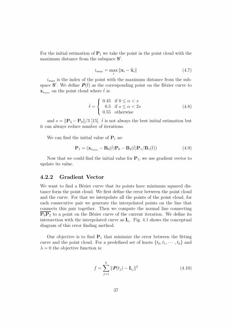
We want to find a Bezier curve that its points have minimum squared dis-tance form the point cloud. We first define the error between the point cloudand the curve. For that we interpolate all the points of the point cloud, foreach consecutive pair we generate the interpolated points on the line thatconnects this pair together. Then we compute the normal line connectingP0P2 to a point on the Bezier curve of the current iteration. We define itsintersection with the interpolated curve as Iti . Fig. 4.1 shows the conceptualdiagram of this error finding method.
Our objective is to find P1 that minimize the error between the fittingcurve and the point cloud. For a predefined set of knots {t0, t1, · · · , tk} andλ = 0 the objective function is:
f =k∑
j=1
‖P(tj)− Itj‖2 (4.10)
37
b
b
bb
b b
b
b b
b
b
P(t)
P0 P2
I ti
Figure 4.1 – The conceptual diagram of error between fitting Bezier curve and thepoint cloud.
As we said to minimize f , we iteratively update P1 by D in each iteration.For ith iteration we have Pi
1 = Pi−11 + D, the redefined objective function is:
f(Pi1) = f(Pi−1
1 + D) =k∑
j=1
‖P(tj)− Itj‖2 (4.11)
To find D we differentiate Eq. (4.11) with respect to D. Then we set itequal to zero.
k∑
j=1
B1(tj)[P(tj)− Itj
]= 0 (4.12)
then
D =
∑kj=1 U(tj)
∑kj=1 B2
1(tj)(4.13)
Where U(tj) = B1(tj)Itj −B0(tj)B1(tj)P0−B1(tj)2P1−B1(tj)B2(tj)P2.
This procedure is iterated until f(·) remains constant. We summarize SingleControl Point Error Minimization curve fitting method in algorithm 4.
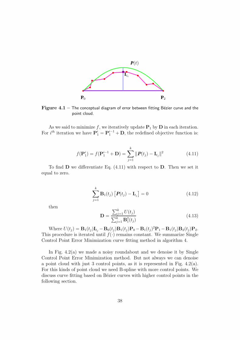
In Fig. 4.2(a) we made a noisy roundabout and we denoise it by SingleControl Point Error Minimization method. But not always we can denoisea point cloud with just 3 control points, as it is represented in Fig. 4.2(a).For this kinds of point cloud we need B-spline with more control points. Wediscuss curve fitting based on Bezier curves with higher control points in thefollowing section.
38
Algorithm 4 Single Control Point Error Minimization1: P0 ← x0
2: P1 ← xk
3: P1 ← (ximax−B0(t)P0 −B2(t)P1/B1(t))
4:
5: while fi > fi−1 do6:
7: D←∑k
j=1 U(tj)/∑k
j=1 B21(tj)
8: Pi1 ← Pi−1
1 + D9: fi ←
∑k
j=1 ‖P(tj)− Itj‖210:
11: end while
28 29 30 31 32 33 34299
300
301
302
303
304
305
306
307
Latitude [m]
Long
itude
[m]
Curve Fitting Using Single Control Point Error Minimization
Point CloudBezier Curve
(a)
−4 −3 −2 −1 0 1 2 3 4−1.5
−1
−0.5
0
0.5
1
1.5
Latitude [m]
Long
itude
[m]
Using Single Control Point Error Minimization
Point CloudBezier Curve
(b)
Figure 4.2 – Using iterative error minimization to fit a Bezier curve with 3 controlpoints to a point cloud 4.2(a) is and example in which Single ControlPoint Error Minimization method works properly. 4.2(b) shows a casethat this fitting algorithm does not work properly.
4.3 Multiple Control Points Error Minimiza-
tion
We previously said because Single Control Point Error Minimization usesB-spline with three control points which does not work properly for manycases. We need a method that we could freely choose number of controlpoints based on maxima and minima of the GPS trajectory. To approxi-mate the scattered GPS data points, we need to starts with a proper initialB-spline and use iterative error minimization toward a best fitting curve tothe point cloud. The advantage of this method is ability to freely choose
39
number of control points. Thus we should have a better approximation withthis method. Moreover, we utilize a new error term which can be devised toyield fast convergence and a better error approximation. Therefore, this errorterm is provided by a curvature-based quadratic approximation of squareddistance of point cloud from the fitting curve [13]. In contrast with SingleControl Point Error Minimization, there is no constraint for the ending con-trol points of B-spline. This also contributes to a better approximation forthe ending of the point could.
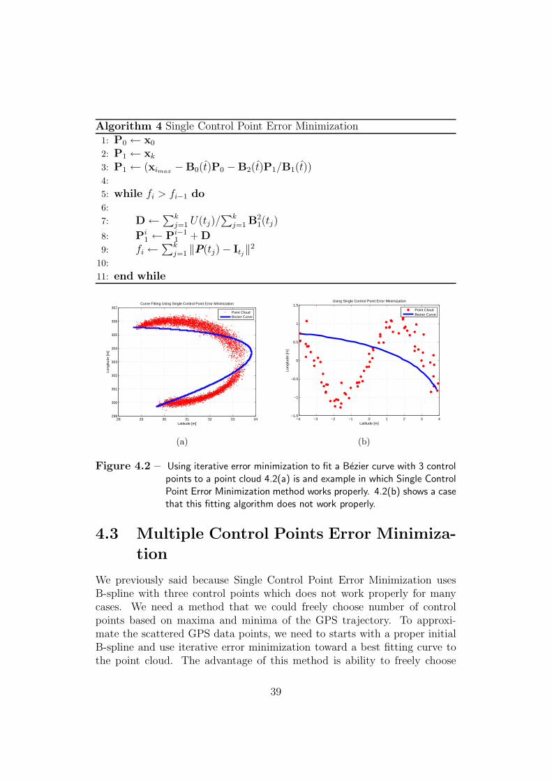
4.3.1 Second Order Approximation of Squared Dis-tance
In Euclidean R2, we consider a curve C(t) with parameter (c1(t), c2(t)). The
normal and tangent vector at each point of the curve C(t) are denoted by N
and T respectively. For each point x the shortest distance to curve C(t) isgiven by d = ‖C(t)− x‖ [9].
b
x0
(0, )
y
x
d
C(t0)
Figure 4.3 – Second order approximation of squared distance function to the curveC(t).
Consider a fixed point x0 and let C(t0) be the normal footprint of x0 onC(t0). In addition, consider the local Frenet frame of C(t0) with its originat c(t0) and its coordinates axes parallel to the tangent and normal vector ofC(t0) at C(t0). Coordinates of x in this axes are (0, d). The coordinates ofcurvature center k(t0) at C(t0) are (0, ) (Fig. 4.3). is radius of C(t0) whichis inverse curvature and has the same sign as the curvature, depending onthe orientation of the curve. Consider a point x = (x, y) in the neighborhoodof x0, then the squared distance from x to C(t) is:
f(x, y) =(√
x2 + (y − )2 − ||)2
(4.14)
40
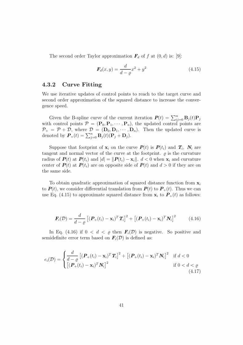
The second order Taylor approximation Fd of f at (0, d) is: [9]:
Fd(x, y) =d
d− x2 + y2 (4.15)
4.3.2 Curve Fitting
We use iterative updates of control points to reach to the target curve andsecond order approximation of the squared distance to increase the conver-gence speed.
Given the B-spline curve of the current iteration P(t) =∑n
ij=0 Bj(t)Pj
with control points P = (P0,P1, · · · ,Pn), the updated control points areP+ = P + D, where D = (D0,D1, · · · ,Dn). Then the updated curve isdenoted by P+(t) =
∑nj=0 Bj(t)(Pj + Dj).
Suppose that footprint of xi on the curve P(t) is P(ti) and Ti, Ni aretangent and normal vector of the curve at the footprint. is the curvatureradius of P(t) at P(ti) and |d| = ‖P(ti)− xi‖. d < 0 when xi and curvaturecenter of P(t) at P(ti) are on opposite side of P(t) and d > 0 if they are onthe same side.
To obtain quadratic approximation of squared distance function from xi
to P(t), we consider differential translation from P(t) to P+(t). Thus we canuse Eq. (4.15) to approximate squared distance from xi to P+(t) as follows:
Fi(D) =d
d−
[(P+(ti)− xi)
TTi
]2+
[(P+(ti)− xi)
TNi
]2(4.16)
In Eq. (4.16) if 0 < d < then Fi(D) is negative. So positive andsemidefinite error term based on Fi(D) is defined as:
ei(D) =
d
d−
[(P+(ti)− xi)
TTi
]2+
[(P+(ti)− xi)
TNi
]2if d < 0
[(P+(ti)− xi)
TNi
]2if 0 < d <
(4.17)
41
4.3.3 Regularization Factor
To have a smooth output of the estimated curve λfs = αF1 + βF2 where5
α, β ≥ 0 and F1, F2 are energy terms defined as:
F1 =
∫‖P′(t)‖2dt, F2 =
∫‖P′′(t)‖2dt (4.18)
4.3.4 Open B-spline
The problem of open curves are with their ending points. If all the end pointscould be projected to the curve, we could easily use our error term. But thereare cases that all points of the point cloud cannot be mapped to a point onthe curve. For these situations we specify a new error term.
(t)
θ
x
P0
0
P
���
���
������
������
���
���
���
���
���
���
���
���
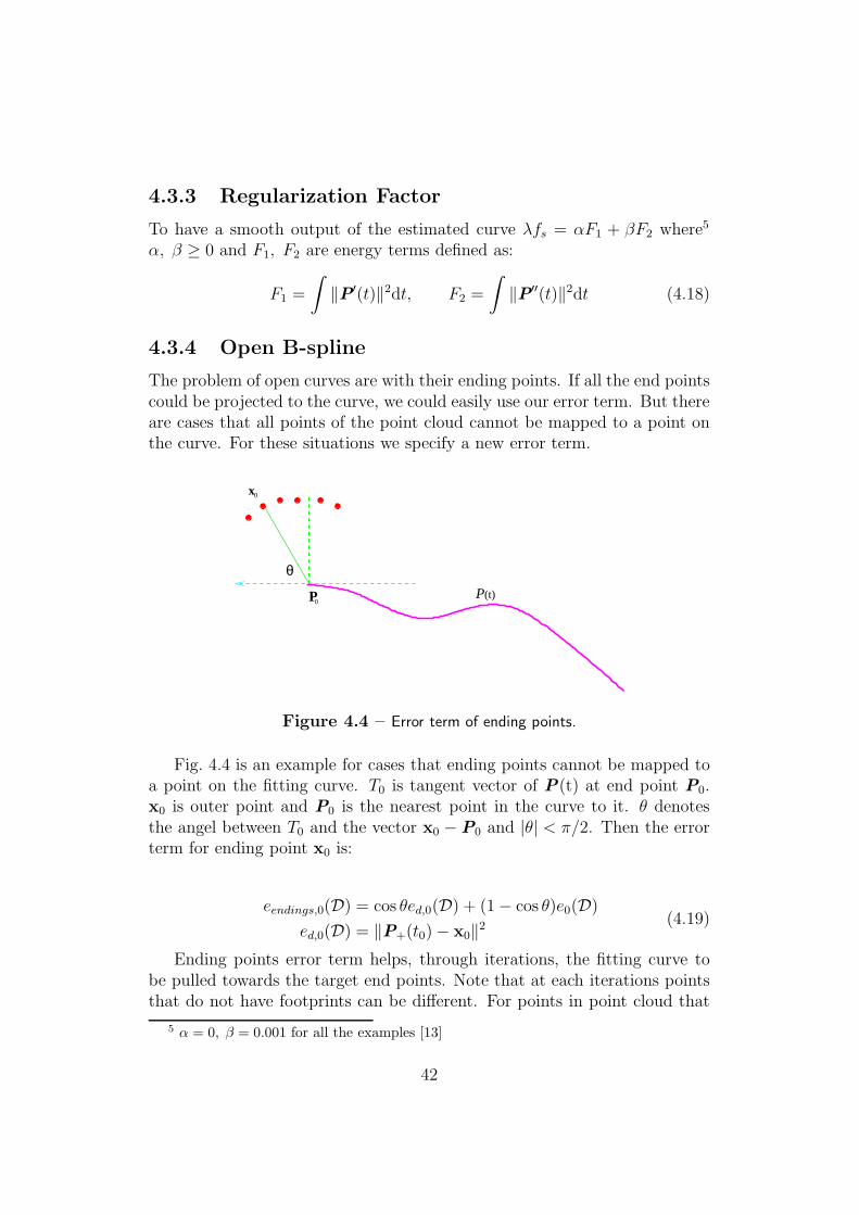
Figure 4.4 – Error term of ending points.
Fig. 4.4 is an example for cases that ending points cannot be mapped toa point on the fitting curve. T0 is tangent vector of P(t) at end point P0.x0 is outer point and P0 is the nearest point in the curve to it. θ denotesthe angel between T0 and the vector x0 −P0 and |θ| < π/2. Then the errorterm for ending point x0 is:
eendings,0(D) = cos θed,0(D) + (1− cos θ)e0(D)
ed,0(D) = ‖P+(t0)− x0‖2(4.19)
Ending points error term helps, through iterations, the fitting curve tobe pulled towards the target end points. Note that at each iterations pointsthat do not have footprints can be different. For points in point cloud that
5 α = 0, β = 0.001 for all the examples [13]
42
we have footprint we use the previous error term.
28 29 30 31 32 33 34299
300
301
302
303
304
305
306
307B−Spline−curve with 5 control points of order 4
Long
itude
[m]
Latitude [m]
Point CloudB−splineRemoved Part
(a)
−6 −4 −2 0 2 4 6 8−6
−4
−2
0
2
4
6
Latitude [m]
Long
itude
[m]
B−Spline−curve with 4 control points of order 4
B−splinePoint CloudRemoved Part
(b)
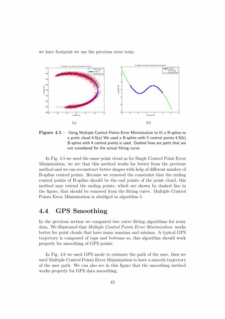
Figure 4.5 – Using Multiple Control Points Error Minimization to fit a B-spline toa point cloud 4.5(a) We used a B-spline with 5 control points 4.5(b)B-spline with 4 control points is used. Dashed lines are parts that arenot considered for the actual fitting curve.
In Fig. 4.5 we used the same point cloud as for Single Control Point ErrorMinimization, we see that this method works far better from the previousmethod and we can reconstruct better shapes with help of different number ofB-spline control points. Because we removed the constraint that the endingcontrol points of B-spline should be the end points of the point cloud, thismethod may extend the ending points, which are shown by dashed line inthe figure, that should be removed from the fitting curve. Multiple ControlPoints Error Minimization is abridged in algorithm 5.
4.4 GPS Smoothing
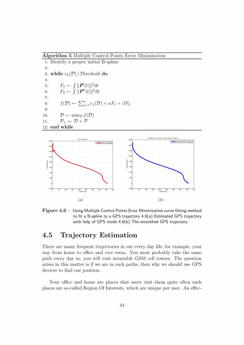
In the previous section we compared two curve fitting algorithms for noisydata. We illustrated that Multiple Control Points Error Minimization worksbetter for point clouds that have many maxima and minima. A typical GPStrajectory is composed of tops and bottoms so, this algorithm should workproperly for smoothing of GPS points.
In Fig. 4.6 we used GPS mode to estimate the path of the user, then weused Multiple Control Points Error Minimization to have a smooth trajectoryof the user path. We can also see in this figure that the smoothing methodworks properly for GPS data smoothing.
43
Algorithm 5 Multiple Control Points Error Minimization
1: Identify a proper initial B-spline2:
3: while ek(D) 〉Threshold do4:
5: F1 ←∫‖P′(t)‖2dt
6: F2 ←∫‖P′′(t)‖2dt
7:
8: f(D)←∑nj=1 ej(D) + αF1 + βF2
9:
10: D ← minD f(D)11: P+ ← D + P12: end while
0 50 100 150 200 250 300 350 400 450−200
0
200
400
600
800
1000
1200
1400
1600
Latitude [m]
Long
itude
[m]
GPS Trajectory
Noisy Trajectpry
(a)
0 50 100 150 200 250 300 350 400 450−200
0
200
400
600
800
1000
1200
1400
1600B−Spline−curve with 6 control points of order 4
Latitude [m]
Long
itude
[m]
Denoised GPS Trajectory
(b)
Figure 4.6 – Using Multiple Control Points Error Minimization curve fitting methodto fit a B-spline to a GPS trajectory 4.6(a) Estimated GPS trajectorywith help of GPS mode 4.6(b) The smoothed GPS trajectory.
4.5 Trajectory Estimation
There are many frequent trajectories in our every day life; for example, yourway from home to office and vice versa. You most probably take the samepath every day so, you will visit invariable GSM cell towers. The questionarises in this matter is if we are in such paths, then why we should use GPSdevices to find our position.
Your office and home are places that users visit them quite often suchplaces are so-called Region Of Interests, which are unique per user. An effec-
44
tive way to obtain ROIs is based on WLANs and GSM cell towers. If the userspends specific time of his day or week seeing certain WLANs or cell towers,the location of the WLANs6 can be one of the user ROIs. This experimentcan be continued until finding all the ROIs. It is also possible to install asoftware on the mobile phone, which is able to store all the ROIs of its owner.
Now that we could find ROIs, it is possible to find the most probablepath that the user travels among his ROIs. Then for the next time that youtravel from one of your ROIs to the other, mobile phone can turn off its GPSsensor and navigate you based on the estimated path that it already has.Navigation is based on history of visited GSM cell towers and compare themwith the current one so, it can predict your position and show your futurepath.
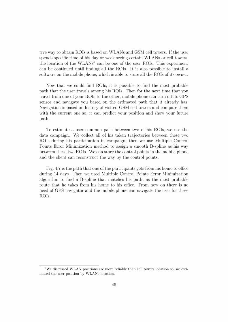
To estimate a user common path between two of his ROIs, we use thedata campaign. We collect all of his taken trajectories between these twoROIs during his participation in campaign, then we use Multiple ControlPoints Error Minimization method to assign a smooth B-spline as his waybetween these two ROIs. We can store the control points in the mobile phoneand the client can reconstruct the way by the control points.
Fig. 4.7 is the path that one of the participants gets from his home to officeduring 14 days. Then we used Multiple Control Points Error Minimizationalgorithm to find a B-spline that matches his path, as the most probableroute that he takes from his home to his office. From now on there is noneed of GPS navigator and the mobile phone can navigate the user for theseROIs.
6We discussed WLAN positions are more reliable than cell towers location so, we esti-mated the user position by WLANs location.
45
0 20 40 60 80 100 120 140 1600
100
200
300
400
500
600
700
800
900
Latitude [m]
Long
itude
[m]
GPS trajectory between 2 ROIs during 14 days
Point Cloud
(a)
0 20 40 60 80 100 120 140 160−100
0
100
200
300
400
500
600
700
800
900
Latitude [m]
Long
itude
[m]
B−Spline−curve with 14 control points of order 4
Estimated Path
(b)
Figure 4.7 – Using Multiple Control Points Error Minimization method to fit aB-spline to paths that a user has taken during 14 days between hisROIs, as his most probable future way. 4.7(a) Routes that the usertraveled during these days from his home to his office 4.7(b) The mostprobable way that the user will take for his next travel between hisROIs.
46
Chapter 5
Conclusion
GPS is widely used in practice for positioning. As we have shown, althoughGPS have been designed in a way to be as accurate as possible, in prac-tice there are some error sources that cause imprecise positioning and weexplained the most common error sources. Moreover, because we deal withGPS receiver of a mobile phone, in which the quality of GPS receiver is notgood, positioning has more error comparing to other GPS receivers. Theother problem with GPS is its availability, that is, GPS is not accessible inplaces that people spend most of their time.
Against these backdrops, we have proposed a novel and efficient position-ing method that does not just depend on GPS. Based on the availability ofthe GPS signal, our proposed method divides into two different operatingmode. For situations that GPS is accessible, we suggested a probability den-sity for GPS points. Locating of the user is based on maximization of jointprobability of GPS points around the time that we want to find the locationof the user. On the other hand, we spend most of our social life in placesthat GPS signal is not available for these kind of situations our proposedalgorithm enters to its second mode of operation. With the help of ongoingdata collection campaign by NRC-Lausanne, we could access to other infor-mation of users except from GPS data. This mode depends on WLANs andGSM cell towers that cover the user. For this mode we firstly should findposition of WLANs and cell towers, WLANs position estimation is basedon the guess that each campaign participant has from his visited WLAN. Ifthe user does not have GPS points for a specific time duration, we use thesecond model and positioning depends on other information than GPS. Wehave shown empirically that our proposed positioning superior performancein both convergence and accuracy.
47
We have also proposed a smoothing algorithm for fitting B-spline curvesto GPS points. The curve fitting algorithm, called Multiple Control PointsError Minimization, makes use of curvature information to give a close ap-proximation of the squared distance function and this contributes to its sim-plicity and efficiency.
In addition, We used Multiple Control Points Error Minimization tosmooth the estimated user trajectory. Interestingly, we have proposed anavigation method among the user’s ROIs that unlike most other navigationsystems does not depend on GPS. For this method we fit a B-spline to themost common path that the user takes among his ROIs. This navigationmethod arises as the consequence of participating in the data collection cam-paign that helps us to have a history of the user’s trajectories.
We expect to see more studies on finding user’s ROIs and the most proba-ble path problems both theoretically and from the view-point of mobile phoneapplications. Although we have tried to consider all the available informationto estimated the user position, an immediate extension is to consider othersources like discovered BTs by mobile phones in each time instance to im-prove the precession of the localization. Other problems include to optimizethe knots and weights of the curve fitting method. In general, to improvethe smoothness of the trajectories by map matching so that they have morecompatibility with actual routes.
48
Bibliography
[1] Shane Ahern, Marc Davis, Simon King, Mor Naaman, and Rahul Nair.Reliable, User-Contributed GSM Cell-Tower Positioning Using Context-Aware Photos. Th Eight International Conference on Ubiquitous Com-
puting, 2006.
[2] Reha Metin ALKAN. GPS-Single Point Positioning Without SelectiveAvailability. In Proceedings of U.S. Hydrographic Conference, pages 22–24. The Hydrographic Society of America, 2001.
[3] Anthony LaMarca1 et al. Place Lab: Device Positioning Using RadioBeacons in the Wild. In Proceedings of the Third International Confer-
ence on Pervasive Computing, pages 116–133, Munich, Germany, 2005.Springer.
[4] Garmin International. About GPS.http://www.garmin.com/aboutGPS/, 2001.
[5] Niko Kiukkonen. Technical Report: Data Collection Campaign. Tech-
nical report, 2009.
[6] Dr. Anja Kohne and Dr. Michael Woßner. Sources of Errors in GPS.http://www.kowoma.de/en/gps/errors.htm, 2009.
[7] Binghao Li, James Salter, Andrew G.Dempster, and Chris Rizos. IndoorPositioning Techniques Based on Wireless LAN. In LAN, First IEEE
International Conference on Wireless Broadband and Ultra Wideband
Communications, pages 13–16, Sydney, Australia, 2006.
[8] Min Mun, Sasank Reddy, Katie Shilton, Nathan Yau, Jeff Burke, Deb-orah Estrin, Mark Hansen, Eric Howard, Ruth West, and Pter Boda.PEIR, The Personal Environmental Impact Report, as a Platform forParticipatory Sensing Systems Research. In International Conference
On Mobile Systems, Applications And Services, pages 55–68, Poland,2009. Association for Computing Machinery.
49
[9] Helmut Pottmann and Michael Hofer. Geometry of the Squared DistanceFunction to Curves and Surfaces. In Visualization and Mathematics III,pages 223–244. Springer, 2003.
[10] Matthew Rabinowitz and Jr. James J. Spilker. A New Positioning Sys-tem Using Television Synchronization Signals. Rosum Corporation white
paper, 2004.
[11] Timothy Sohn, Alex Varshavsky, Anthony Lamarca, Mike Y. Chen,Tanzeem Choudhury, Ian Smith, Sunny Consolvo, Jeffrey Hightower,William G. Griswold, and Eyal De Lara. Mobility Detection Using Ev-eryday GSM Traces. In Proceedings of the Eighth International Confer-
ence on Ubiquitous Computing, pages 212–224. Springer, 2006.
[12] Martin Vetterli and Jelena Kovacevic. Wavelets and Subband Coding ,pages 25–27. Prentice Hall, USA, 2007.
[13] Wenping Wang, Helmut Pottmann, and Yang Liu. Fitting B-SplineCurves to Point Clouds by Squared Distance Minimization. ACM Trans-
actions on Graphics, 25, 2004.
[14] Ji wung Choi and Gabriel Hugh Elkaim. Bezier Curve for TrajectoryGuidance. World Congress on Engineering and Computer Science, 2008.
[15] Junyeong Yang and Hyeran Byun. Curve Fitting Algorithm Using It-erative Error Minimization for Sketch Beautification. In International
Conference on Pattern Recognition, Florida, USA, 2009.
[16] Daniel Zwillinger. Standard Mathematical Tables and Formulae , pages32–35. CRC Press, 30th edition, 1996.
50