Estimating a Model of Excess Demand for Public

Housing

J. Geyer

Abt Associates

H. Sieg

University of Pennsylvania and NBER

April 16, 2013

Abstract

The purpose of this paper is to develop and estimate a new equilibrium model of

public housing that acknowledges the fact that the demand for public housing may

exceed the available supply. We show that ignoring these supply side restrictions leads

to an inconsistent estimator of household preferences. We estimate the parameters of

the model based on a unique panel data set of low-income households in Pittsburgh.

We find that public housing is an attractive option for seniors and exceedingly poor

households headed by single mothers. We also find that for each family that leaves

public housing there are on average 3.8 families that would like to move into the

vacated unit. Simple logit demand models that ignore supply side restrictions cannot

generate reasonable wait times and wait lists. Demolitions of existing units increase

the degree of rationing and potentially result in welfare losses. An unintended conse-

quence of demolitions is that they increase racial segregation in low income housing

communities.

Keywords: Excess Demand, Rationing, Search, Equilibrium Analysis, Welfare Anal-

ysis, Enriched Sampling, Computational General Equilibrium Analysis.

JEL classification: C33, C83, D45, D58, H72, R31.

1 Introduction

Providing adequate housing and shelter for low income households is a stated policy

goal of most administrations in the United States and Europe. One important policy,

implemented by the Department of Housing and Urban Development (HUD), subsi-

dizes the construction and maintenance of affordable housing communities in cities

and metropolitan areas in the U.S.1 Low income households are eligible for public

housing assistance in the U.S. if their income is below a threshold that depends on

household composition and region. Given the current standards for determining el-

igibility, there is typically a large number of households in each metropolitan area

eligible for public housing.

Supply of public housing units is primarily determined by current and past po-

litical decisions that have allocated funding to local housing authorities. Since the

rent charged for public housing is a fixed percentage of household income, there is no

price mechanism to ensure that public housing markets clear. When the demand for

public housing exceeds supply, there are long wait lists to get into public housing. As

a consequence, we cannot use standard demand models to estimate the preferences

for public housing. The purpose of this paper is to develop and estimate a new model

of demand for public housing that acknowledges the fact that the demand for public

housing may exceed the available supply. We show that ignoring these supply side

restrictions leads to inconsistent estimators of household preferences.

There are long wait-lists for public housing in many metropolitan areas. While

we can obtain some aggregate summary statistics that broadly measure the average

wait time in these markets, these aggregate statistics are not sufficient to estimate a

1Low-income housing programs in the United States grew out of the demand to address threats

to public health and safety that resulted from low-cost, high-density housing neighborhoods for

poor, mostly immigrant, families in the early twentieth century. Similar government institutions

and programs exist in most European countries.

1

model that captures heterogeneity across households. Local housing authorities are

not willing to disclose detailed micro-level data on wait lists. To our knowledge, there

is no empirical research that uses household level, wait list data to study rationing

in public housing markets. The key challenge is, therefore, to estimate a model that

treats the wait list as latent.

We develop an equilibrium model that incorporates supply restrictions that arise

from the administrative behavior of the local housing authority. A household can

move into public housing if and only if the housing authority offers the household

a vacant apartment. The ability of the housing authority to offer apartments to

eligible households is largely determined by voluntary exit decisions of households

that currently live in housing communities. Exit from public housing is a stochastic

event since it is partially determined by idiosyncratic preference and income shocks

that are not observed by administrators. The housing authority’s objective is to fill

all vacant units. If the potential demand exceeds the available units at any point of

time, the housing authority has to ration access to public housing.

Eligible households that have not been offered an apartment in an affordable

housing community are placed in our model on a wait list. Each period, a fraction of

households on the wait list will receive an offer to move into one of the apartments

that has recently become available. If the total supply of public housing is fixed,

and vacancy rates are constant over time, the housing authority adjusts the offer

probabilities in equilibrium so that the inflow into public housing equals the voluntary

outflow. We define an equilibrium for our model and characterize its properties. We

show that there exists a unique equilibrium if there are no transfers between public

housing communities. If transfers are possible, the equilibrium is also unique as long

as the housing authority adopts an equal treatment policy.

We show how to identify and estimate the parameters of the model using data on

observed choices, but unobserved wait lists. Since we do not observe the wait list,

2

we do not know which households received offers to move into housing communities.

We only observe those offers that were accepted and resulted in a move.2 The basic

insight of our identification approach is that offer probabilities are endogenous and

are constrained to satisfy equilibrium conditions. Hence, offer probabilities can be

expressed as functions of the structural parameters of the housing choice models.

Moreover, exit is purely voluntary and does not depend on offer probabilities. As

a consequence, exit behavior is informative about the structural parameters of the

utility function. Imposing the equilibrium conditions then establishes identification

of the structural parameters of the model.

We estimate the model using a unique data set from the Housing Authority of the

City of Pittsburgh (HACP).3 We supplement these data with a sample of eligible low

income households in the Survey of Income and Program Participation which allows

us to follow eligible households outside of public housing.

We find that households that have income well below the poverty line and are

headed by single mothers have strong preferences for public housing. African Amer-

ican households also have strong public housing preferences. The income coefficient

shows that there are strong incentives for households to leave public housing as their

income grows larger. These incentives are off-set by the presence of significant moving

costs that constrain potential relocations of households. We find that for each family

that leaves public housing there are on average 3.8 families that would like to move

into the vacated unit. For seniors, the rationing is more pronounced. For each senior

that moves out of a housing community there are 23.2 senior households that would

2This type of selection problem is also encountered in labor search and occupational choice

models. For a discussion of identification and estimation of labor search model see, among others,

Eckstein and Wolpin (1990) and Postel-Vinay and Robin (2002). Heckman and Honore (1990)

discuss identification in the Roy model.3Olsen, Davis, and Carrillo (2005) use restricted use data from HUD to study the impact of

variations in local housing policies on household behavior.

3

like to move in.

Finally, we conduct some counterfactual policy experiments. We evaluate a pol-

icy that considers the demolition of some of the existing public housing units. We

find that the welfare costs of demolishing even the least desirable units are substan-

tial. Displaced African American females are disproportionately disadvantaged, which

raises some serious issues related to the distributional impact of these demolition

programs. An unintended consequence is that the resulting equilibrium demographic

distribution in the remaining public housing communities exhibits some increase in

the proportions of female and African American residents, and thus an increase in

segregation in these already highly segregated communities.

The remainder of the paper is organized as follows. Section 2 introduces our

data set. Section 3 provides an equilibrium model that treats public housing as a

differentiated product that is subject to rationing. Section 4 discusses identification

and derives the maximum likelihood estimator for this model. The empirical results

are presented in Section 5. Section 6 conducts some counterfactual policy analysis.

We offer some conclusions in Section 7.

2 Institutional Background and Data

The U.S. Housing Act of 1937 formed the U.S. Public Housing Program that funds

local governments in their ownership and management of buildings to house low-

income residents at subsidized rents.4 The U.S. government pursued an active policy

of constructing public housing communities during the 1950’s and 1960’s. The Reagan

administration significantly reduced financing for the construction of new housing

projects during the 1980’s in order to shift the focus to creating to voucher programs.

4Olsen (2001) provides a detailed description of the history and current practices of the various

different U.S. Public Housing Programs.

4

Since the early 1990s, HUD has given financial incentives under HOPE VI and related

programs to tear down projects that are considered to be distressed.

New programs to encourage construction of privately-owned low income housing

emerged as construction of public housing ceased and demolition of public housing

began. As detailed in Erickson and Rosenthal (2011), the Low Income Housing Tax

Credit (LIHTC) program was created in 1986 as part of the Tax Reform Act of 1986 as

an alternative to public housing. They observe that ”LIHTC has quickly overtaken all

previous place-based subsidized rental programs to become the largest such program

in the nations history.” They find, however, that this program has failed to result in

new construction that serves the population served by public housing, largely due to

crowd-out effects. As a consequence, there is not an adequate supply of affordable

housing and there are long wait lists to get access to public housing in many U.S.

cities.5

Currently, the U.S. Department of Housing and Urban Development funds the

efforts of hundreds of city and county housing authorities in the United States. In

Pennsylvania alone, there are 92 distinct housing authorities. In 2006, the estimated

HUD budget for public housing was $24.604 billion.6 Within the public housing

program, this funding supports administration, building maintenance, and even law

enforcement.

The empirical analysis presented in this paper focuses on communities owned and

managed by the Housing Authority of the City of Pittsburgh. In 2005 HUD provided

5There is some evidence suggesting negative spill-over effects (such as higher crime rates and lower

educational achievement) associated with living in public housing (Oreopoulos, 2003). However,

Jacob (2004) who considers the impact of demolitions in Chicago finds that there are very few

positive effects associated with moving out of the projects using a variety of different outcomes.6HUD (2007) provides details. Note that this figure does not include housing voucher programs,

low-income community development programs, or other none-state owned and managed housing

programs.

5

the HACP with $83.7 million in grants for public housing, housing vouchers, and other

programs. In the same year, HACP received $8.3 million from tenant payments. Only

a small number public housing communities were demolished during the course of our

survey.7 As a consequence the supply of public housing has been approximately fixed

during our study period.

The public housing stock in the City of Pittsburgh is heterogeneous, including

small houses converted into several apartment units, large high-rises, and large com-

munities of low-rise housing spread continuously over several blocks offering as many

as 600 units. These communities are usually designated as either ’family’ communi-

ties or ’senior’ communities, where senior communities target households age 62 or

older. There are 34 separate sites. 19 of these sites are family units, 11 are designated

for seniors and 4 of them have both senior- and family-designated units. There are

16 large communities with more than 100 units, 8 are medium sized, and 10 are small

with less than 40 units. Heterogeneity in public housing also arises due to differences

in local amenities. The 34 public housing communities in the HACP are located

across 19 of Pittsburgh’s 32 wards and across 28 census tracts. These public hous-

ing communities also vary in terms of neighborhood amenities such as crime, school

quality, property values and demographic characteristics.8

7Much of the demolition was motivated by the argument that growing up in public housing

might be negative for children, although this conjecture is controversial in the literature (Currie and

Yelowitz, 2000). For an analysis of the the impact of public housing demolitions in Chicago see

Jacob (2004).8There is much evidence that suggests that households make residential decisions based on neigh-

borhood characteristics and local public goods. This evidence is based on estimated locational equi-

librium models such asEpple and Sieg (1999), Epple, Romer, and Sieg (2001), Sieg, Smith, Banzhaf,

and Walsh (2004), Calabrese, Epple, Romer, and Sieg (2006), Ferreyra (2007), Walsh (2007), and

Epple, Peress, and Sieg (2010). Bergstrom, Rubinfeld, and Shapiro (1982), Rubinfeld, Shapiro, and

Roberts (1987), Nesheim (2001), Bajari and Kahn (2004), Bayer, McMillan, and Reuben (2004),

Schmidheiny (2006), Bayer, Ferreira, and McMillan (2007), and Ferreira (2009) are examples of

related empirical approaches which are based on more traditional discrete choice models or hedonic

6

The HACP data contain records of household entry, exits, and transfers from June

2001 to June 2006 within the 34 public housing communities actively used during this

time period. The data set also includes annual updates of each of these households

as well as any non-periodic reports that update information about household compo-

sition or pre-rent income that is reported to the HACP. These records contain most

of the information fields requested of all U.S. housing authorities including age, race,

household composition including age and relationship of family members and house-

mates, earnings, and income adjustment exclusions including disability, medical, and

childcare expenses. We also observe the monthly rent being charged to a particular

household, the number of bedrooms of the housing unit, whether the community is

targeted to seniors, and the address and unit number. There are 7,070 households

observed at least once during this time period; there are 2,907 households that move

in for the first time, 3,155 households that move out, and 1,244 that transfer from

one public housing unit to another.

Table 1 summarizes key descriptive statistics for the full sample and for four sub-

samples that are differentiated by community type. Although some families live in

senior housing and some seniors live in non-senior housing, age and family composition

distributions are bimodal with respect to these two types of communities. In mixed

communities, demographic variables look similar to a weighted average of senior and

family communities, however there are more cohabiting adults and a higher number of

children in mixed housing than in family-only or senior-only housing. The mean age

in senior housing is 31 years greater than the mean age in non-senior housing. The

majority of households in both senior-only and family-only communities are female,

but females are a much larger majority in family-only communities. African American

households are a very high proportion of residents in family and mixed housing, while

senior units have nearly equal proportions of African American and White households.

frameworks.

7

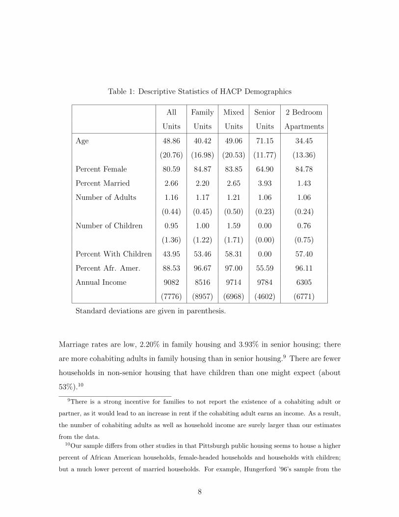
Table 1: Descriptive Statistics of HACP Demographics

All Family Mixed Senior 2 Bedroom

Units Units Units Units Apartments

Age 48.86 40.42 49.06 71.15 34.45

(20.76) (16.98) (20.53) (11.77) (13.36)

Percent Female 80.59 84.87 83.85 64.90 84.78

Percent Married 2.66 2.20 2.65 3.93 1.43

Number of Adults 1.16 1.17 1.21 1.06 1.06

(0.44) (0.45) (0.50) (0.23) (0.24)

Number of Children 0.95 1.00 1.59 0.00 0.76

(1.36) (1.22) (1.71) (0.00) (0.75)

Percent With Children 43.95 53.46 58.31 0.00 57.40

Percent Afr. Amer. 88.53 96.67 97.00 55.59 96.11

Annual Income 9082 8516 9714 9784 6305

(7776) (8957) (6968) (4602) (6771)

Standard deviations are given in parenthesis.

Marriage rates are low, 2.20% in family housing and 3.93% in senior housing; there

are more cohabiting adults in family housing than in senior housing.9 There are fewer

households in non-senior housing that have children than one might expect (about

53%).10

9There is a strong incentive for families to not report the existence of a cohabiting adult or

partner, as it would lead to an increase in rent if the cohabiting adult earns an income. As a result,

the number of cohabiting adults as well as household income are surely larger than our estimates

from the data.10Our sample differs from other studies in that Pittsburgh public housing seems to house a higher

percent of African American households, female-headed households and households with children;

but a much lower percent of married households. For example, Hungerford ’96’s sample from the

8

Table 2: Descriptive Statistics of the SIPP Subsample Compared to Census and

HACP

Census SIPP SIPP SIPP HACP

All All Private Public Public

Age 50.83 52.70 52.72 52.19 48.86

Percent Female 54.6% 59.94% 59.06% 76.56% 80.59%

Percent Married 22.6% 30.79% 32.09% 6.25% 2.66%

Number of Adults 1.450 1.274 1.284 1.094 1.160

Number of Children 0.495 0.617 0.616 0.641 0.950

Percent With Children 24.73% 30.32% 30.27% 31.25% 43.95%

Percent Afr. Amer. 32.64% 28.28% 27.05% 51.56% 88.53%

Annual Income $14,079 $18,979 $19,391 $11,184 $9,082

“All” refers to all eligible households in the sample.

“Private” refers to all eligible households in the sample in private housing.

“Public” refers to all eligible households in the sample in public housing.

9

In the HACP data we only observe households that have lived in public housing

at some point during the sample period. Once households leave the housing commu-

nities, the HACP does not conduct any follow-up surveys. To learn about households

that are eligible for public housing, but do not live in one of the housing communities,

we turn to the 2001 Survey of Income and Program Participation (SIPP). The SIPP

is a survey managed by the U.S. Census Bureau that interviews households every

four months for 3 years. Each month, households are asked about their previous four

months’ family composition, sources of income, and participation in government pro-

grams such as public housing and school lunch programs. We create a sample based

on the SIPP that contains households eligible for housing aid.11

Table 2 provides some descriptive statistics for our SIPP sample used in this anal-

ysis and compares it to Census and HACP data. We find that low-income households

that rent in the private market are on average more likely to be married, are less

likely to be African American, and have substantially higher income than households

in public housing. Comparing the SIPP with the HACP sample we find that the SIPP

sample is slightly older, average income is slightly higher, and children are fewer than

in the HACP. Comparing the SIPP with the Census, the SIPP contains slightly older

heads of household, more female heads of household, more married householders,

households with more children, and fewer African American households. However,

the differences between the SIPP sample and the Census sample of eligible households

1986-1988 SIPP panel was 52% female, 23% African American, 32% married and the mean number

of children was 0.21 (Hungerford, 1996).11The SIPP contains only 14 households that participate in public housing in Pittsburgh at some

point during the sample period. There are 156 Pittsburgh households eligible for public housing in

the first quarter. We construct a subsample of the SIPP using the unweighted data of households

eligible for public housing who live in metropolitan areas similar to Pittsburgh. Appendix B contains

information on how the SIPP sample was constructed and compares characteristics of Pittsburgh

with characteristics of the metropolitan areas selected in our SIPP subsample.

10

in Pittsburgh are relatively small.12

Table 3: Transition Matrix

Private PH 1 PH 2 PH 3 PH 4 PH 5 PH 6 Freq

Private 0 677 144 24 300 59 191 1395

PH 1 855 16264 16 2 75 7 10 17229

PH 2 233 16 5371 3 17 8 7 5655

PH 3 44 2 29 1438 1 0 2 1516

PH 4 572 16 8 1 12156 5 9 12767

PH 5 105 1 0 0 1 2017 29 2153

PH 6 302 0 0 1 47 37 8129 8516

Rows indicate choices in t− 1 and columns in t.

Freq: indicates row frequencies.

The 34 communities are classified into broad community types: family large (PH

1), family medium (PH 2), family small (PH 3), mixed (PH 4), senior large (PH

5), and senior small (PH6). These six types of housing units are fairly homogenous,

but seem to attract different types of households. Large, medium, and small low-

rise non-senior communities primarily house families with children. Most senior-

dominated communities include a significant percentage of non-senior adults without

kids ranging from 13% to 37%. Most family-only communities include some senior

households ranging from 0 - 20%, about a third of which are caring for children.

Table 3 shows the transition matrix for the HACP data. We find that locational

choices are persistent since most households stay with their past choices. However, the

off-diagonal elements of the transition matrix indicate that there is a fair amount of

entry into and exit from public housing.13 Moreover, there are a number of transitions

12See Appendix B.13The HACP does not record the reason or next destination of a household that moves out.

11

within public housing communities. These transfer are largely voluntary and indicate

that household differentiate among the heterogeneous community types.14

3 An Equilibrium Model of Public Housing

3.1 The Baseline Model

We consider a model with a continuum of low-income households. Each household is

eligible for housing aid and can thus, in principle, live in one of the available public

housing communities or rent an apartment in the private market. Denote the outside

private market option with 0. Let J be the number of different housing communities

that are available in the public housing program. Let djt ∈ {0, 1} denote an indicator

variable which equals one if the household chooses alternative j at time t and zero

otherwise.15 Let the vector dt = (d0t, ..., dJt) characterize choices of a household at t.

Since the alternatives are mutually exclusive, we have

J∑j=0

djt = 1 (1)

In our baseline model we do not allow households to move or transfer between units

in different public housing communities.16

Households differ along a number of characteristics xt such as income, age, number

of kids, number of adults, gender of household head, marital status, and race. We

treat these characteristics as exogenous. While it is not difficult to endogenize income

or family status from a conceptual perspective, it significantly increases the difficulty

14In the SIPP sample, we observe 89 transitions from private to public housing and 98 transitions

from public to private housing.15In our application, we use quarterly data.16We relax this assumption in Section 3.2 and consider an extended version of the model with

transfers between units in different communities.

12

of computing equilibria.17

Household preferences are subject to idiosyncratic shocks denoted by εi,t. We

assume that these shocks are continuous random variables with support over the real

line. Moreover, in the baseline model they are i.i.d. across observations and time.18

Households face relocation costs if they decide to move. Thus lagged choices,

denoted by dt−1, are relevant state variables.

Households have preferences defined over all potential elements in the choice set.

We model household preferences using a standard random utility specification.

Assumption 1 Let u(dt, xt, dt−1, εt) denote the household utility function. We as-

sume that the utility function is additively separable in observed and unobserved state

variables and thus allows the following representation:

u(dt, xt, dt−1, εt) =J∑

j=0

djt [uj(xt, dt−1) + εjt] (2)

This specification implicitly treats public housing as a differentiated product.

A key feature of our model is that all potential choices may not be available to

a household at any given point of time. A household that is currently renting in the

private market may not have access to public housing even if the household meets all

eligibility criteria.19 We, therefore, need to formalize the fact that access to public

housing is restricted by a local housing authority.

17We do not observe labor supply or job market participation in the HACP data which is a

limitation of our data set. See Jacob and Ludwig (2010) for analysis of the impact of Section 8

vouchers on income.18One concern with this assumption is that it is plausible that households may have an overall

preference for the public versus the private sector. One way to address this concern is to use a

nested logit specification to capture correlation in unobserved preferences among public housing

communities. We, therefore, also explore this specification as part of our robustness analysis.19In practice, all eligible households are typically assigned to a waiting list. A household will only

receive an offer to move into public housing if it is on top of the waiting list.

13

Assumption 2 The public housing authority does not evict any households that have

lost eligibility.

This assumption is motivated by policies that are typically used by many local hous-

ing authorities. It implies that exit from public housing is purely voluntary. To

characterize the voluntary outflow, let Pjt denote the fraction of eligible households

living in community j at the beginning of period t. The outflow from public housing

community j to the private sector, OFj0t, is defined as:

OFj0t = Pjt

∫Pr(u0(xt, dt−1) + ε0t ≥ uj(xt, dt−1) + εjt) f(xt|djt−1 = 1) dxt (3)

where f(xt|djt−1 = 1) denotes the conditional density function of households with

characteristics xt that live in j at the beginning of period t. As a consequence, the

housing authority faces a stream of housing units that become available at each point

of time. The authority needs to assign these units to new renters. To model this

decision process, we need to model the potential demand for public housing.

Let P0t denote the fraction of eligible households renting in the private market at

the beginning of period t. We make the following assumption:

Assumption 3 All eligible households that are renting in the private market are

placed on a wait list for public housing.

We offer four observations regarding this assumption. First, signing up for the

wait list is, for all practical purposes, costless in practice.20 Second, it is easy to relax

the assumption and allow for systematic differences between households on the wait

list and eligible households that have not signed up on the wait list. When we discuss

the rationing implications, we relax this assumption and consider a case in which a

demand signal triggers households to sign up on the wait list. Third, the assumption

20Of course, it does not matter that all eligible households sign up as long as there are no systematic

differences between eligible households and households on the wait-list.

14

can be justified by empirical constraints. We do not observe the characteristics of

all households on the wait list and neither does the housing authority. We also do

not observe the priority ranking of households on the wait-list. Assumption 3 implies

that the households that have top priority on the wait-list do not systematically differ

from the eligible population.21 Finally, it is also straight forward to assume that the

housing authority has multiple wait lists for households with different family sizes.22

Next consider the potential demand for public housing. The probability that a

households that is currently living in the private sector prefers j at time t is:

Pr(djt = 1|xt, d0t−1 = 1) = Pr(uj(xt, dt−1) + εjt ≥ u0(xt, dt−1) + ε0t) (4)

Let f(xt|d0t−1 = 1) denote the conditional density function of households with char-

acteristics xt that currently rent in the private market, are eligible for public housing,

and thus have been assigned to a wait list. The potential demand for community j is

then characterized by the fraction of households on the wait list that prefer j at time

t:

F0jt = P0t

∫Pr(djt = 1|xt, d0t−1 = 1) f(xt|d0t−1 = 1) dxt (5)

The most interesting case arises if demand exceeds supply. We therefore make the

following assumption:

Assumption 4 a) The potential demand exceeds the voluntary outflow for each com-

munity at each point of time. b) The authority offers the available units to households

on the wait list that have the highest priority. c) The housing authority continues of-

fering units until all available vacant units have been filled with eligible households.

Assumptions 4a and 4b are not necessary to obtain a well defined equilibrium, but

they hold empirically in almost all large markets in the U.S. Assumption 4a implies

21As a consequence, we can solve and estimate the model without observing the conditional

distribution of households on the wait list.22We discuss these issues when we estimate the model in Section 5.

15

that the housing authority cannot meet the full demand. Instead it can only offer

public housing to a fraction of households that are eligible. Assumption 4b implies

that that housing authority follows a first-in-first-out policy. Assumptions 2 through

4 imply that there is a fraction of households, denoted by Π0jt, that will receive offers

to move into housing community j at time t. The total inflow into public housing is

then given by:

IFjt = Π0jt F0jt (6)

We also need to impose an assumption on the supply of public housing and the

vacancy rates.

Assumption 5 The supply of public housing is constant in each housing community

at each point of time.

We can relax this assumption and allow for exogenous changes in the supply of public

housing due new construction or demolitions. We discuss these issues in detail when

we quantify the impact of demolitions in Section 6 of the paper.

Assumption 5 then implies that the outflow must equal the inflow for each housing

community at each point of time in equilibrium.23

IFjt = OFjt (7)

To close the model and define an equilibrium, we need to make an assumption

about initial conditions:

23The assumption of a constant housing stock is common in many theoretical papers that study

housing market equilibrium in urban metropolitan areas. See, for example, Nechyba (1997a, 1997b),

Nechyba (2003), Bayer and Timmins (2005), and Ferreyra (2007).

16

Assumption 6 We take the initial distribution of households at the beginning of

period 1, which is fully characterized the vector of probabilities P1 and conditional

densities f(x1|di,0 = 1) as exogenously determined.

Given Pt and f(xt|di,t−1 = 1), the conditional choice probabilities Pr(djt =

1|xt, dit−1 = 1) then uniquely determine the unconditional choice probabilities Pt+1

and the conditional distribution functions f(xt+1|di,t = 1) that characterize the com-

position of households for each element in the choice set at the beginning of the next

period. Since households are myopic we can define an equilibrium for each point of

time t. The sequence of one-period equilibria is linked by the law of motion that

characterizes the composition of the public housing communities over time.24

An equilibrium for period t for the baseline model can, therefore, be defined as

follows:

Definition 1 Given an initial distribution of household at the beginning of period t,

denoted by Pt and f(xt|dj,t−1), an equilibrium of this model consists of a vector of

probabilities Π01t, ...Π0Jt that such:

• The housing authority offers a fraction Π0jt of all households on the wait list

the opportunity to move into community j.

• Households maximize utility subject to the effective choice set.

• For each housing community, the inflow of households equals the outflow of

households for each housing community as required by equation (7).

We have the following result characterizing existence and uniqueness of equilib-

rium:

24We are abstracting here from households entering or leaving the local economy. It is straight-

forward to account for that.

17

Proposition 1 If the potential inflow exceeds the voluntary outflow for each commu-

nity, then there exists a unique housing market equilibrium with rationing.

Proof:

For each time period, equation (7) implies that equilibrium is defined by a linear sys-

tem of equations with J market clearing conditions and J unknown offer probabilities.

The equilibrium offer probabilities are then ratios of the potential demand given by

the right hand side of equation (6) and the outflow given by equation (3). We assume

that the potential demand exceed at each point of time the voluntary outflow. As a

consequence the offer probabilities are all strictly less than one. Q.E.D.

3.2 An Extended Model with Transfers

We generalize our model and allow for transfers between public housing units. Trans-

fers imply that the demand for public housing must be modified since households may

have additional options. The probability that a households that lives in community

i at the beginning of the period prefers to move to community j at time t is:

Pr(djt = 1|xt, dit−1 = 1) = Pr(uj(xt, dt−1) + εjt ≥ max [ui(xt, dt−1) + εit, u0(xt, dt−1) + ε0t]) (8)

Note that households only compare options that in the effective choice set, i.e. that

are available to them. As before, the potential demand is then characterized by the

fraction of households living in community i that prefer j at time t:

Fijt = Pit

∫Pr(djt = 1|xt, dit−1 = 1) f(xt|dit−1 = 1) dxt (9)

In contrasts to entry into public housing and exit, there is no stated policy for

transfers between public housing units. Nevertheless, we observe a fair number of

transfers in practice. A useful modeling approach is then to mimic our assumptions

imposed on the (external) wait list to generate a well defined transfer policy. Suppose

18

that the housing authority also has an internal mechanism that determines transfer

offers. In that case, a fraction of households that is currently living in i are offered

the opportunity to transfer to community j.

Assumption 7 The probability of obtaining an offer to move into housing commu-

nity j while living in public housing i is given by Πijt. Households get, at most, one

offer at each point of time.

The total realized demand (or inflow) from community i to community j at time

t is therefore Πijt Fijt. Summing over all current housing choices other then j gives

the total inflow into housing community j:

IFjt =J∑

i=0,i 6=j

Πijt Fijt (10)

Similarly we can modify the equation that characterizes the total voluntary outflow

from community j:

OFjt = OFj0t +J∑

i=1,i 6=j

Πjit Fjit (11)

where the outflow to the private sector, OFj0t, is defined as:

OFj0t = Pjt Πjjt

∫Pr(u0(xt, dt−1) + ε0t ≥ uj(xt, dt−1) + εjt) f(xt|djt−1 = 1) dxt

+ Pjt

K∑k=1,k 6=j

Πjkt

∫Pr(u0(xt, dt−1) + ε0t ≥ max [uj(xt, dt−1) + εjt, uk(xt, dt−1) + εkt])

f(xt|djt−1 = 1) dxt (12)

In the extended model we have J2 offer probabilities and J market clearing conditions.

Moreover, the system of equations which defines equilibrium is linear in the offer

probabilities. An equilibrium for the economy exists if the linear system of market

clearing equations has a solution. These solutions (generically) exist, but are not

unique, since the number of equations is smaller than the number of unknowns.25

25See, for example, the discussion in Strang (1988).

19

The potential for multiplicity in equilibrium arises because we have not sufficiently

restricted the ability of the housing authority to allow households to transfer between

different units. There are many transfer policies that are consistent with equilibrium

in the public housing market. The market clearing conditions alone do not uniquely

determine the offer probabilities. To obtain a unique solution to this system of equa-

tions, we need to impose additional assumptions. It is plausible that the housing

authority does not discriminate based on current residence and uses the same odds

ratio for insiders and outsiders. We therefore assume that:

Assumption 8 The fraction of households that receive an offer to transfer between

units in different communities does not depend on current residence:

Πijt = Πjt i = 1, ..., J (13)

The odds ratios are the same for household inside and outside of public housing:

Π0jt = R0t Πjt (14)

Note that this assumption is plausible since housing authorities are not allowed to

discriminate based on income, race, and gender. As a consequence it is hard to believe

that they could discriminate based on residency. The parameter R0t measures the

relative degree of preferential treatment that is given to outsiders. In practice R0t

should much larger than one. As a consequence households on the wait list get pref-

erential treatment over households that are already in public housing. Substituting

Assumption 7 into the definition of equilibrium, we obtain:

R0t Πjt F0jt +∑i 6=j

Πjt Fijt = OFj0t +∑i 6=j

Πit Fjit (15)

which is a system of J equations in J + 1 unknowns. Thus the equilibrium conditions

define the offer probabilities up to the factor R0t. We have, therefore, shown the

following result:

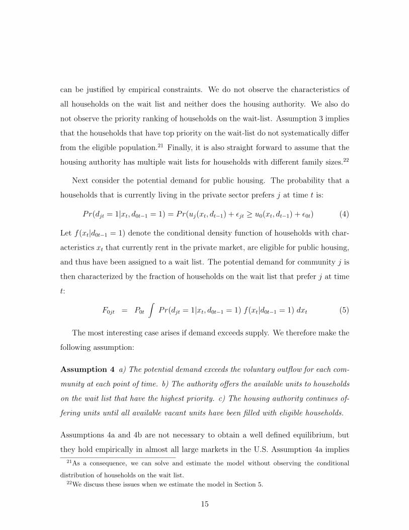
20

Proposition 2 For each value of R0t, there exists a unique housing market equilib-

rium with rationing.

In summary, we have developed an equilibrium model of public housing that gen-

erates rationing and excess demand in equilibrium. The model also explains transfers

between heterogeneous housing communities. One key simplifying assumption of the

model is that we treat households as myopic. If households are forward looking, they

need to forecast, if and when they are offered units in public housing. As a conse-

quence, the value functions and the demand for public housing depend on expectations

about future offer probabilities. The equilibrium can no longer be characterized by

a sequence of one period equilibria. As a consequence, the equilibrium is much more

difficult to characterize and to compute.

4 Identification and Estimation

We estimate the model using two different samples. The first sample is a choice based

sample that is provided by a local authority. This sample tracks households as long

as they stay in public housing. The second sample is a random sample of households

that are eligible for housing aid. In this section we introduce a parametrization

of our model. We then derive the conditional choice probabilities and develop our

maximum likelihood estimator. We then discuss the role that equilibrium conditions

play in establishing identification of the model. Finally, we show that our approach

works in a Monte Carlo study when the data generating process is known.

4.1 A Parametrization

We assume that the utility associated with community j is given by

ujt = γj + β ln(yjt) + δxt + mc 1{dt 6= dt−1} + εjt j = 1, ..., J (16)

21

The utility of the outside option is normalized to be equal to the following expression:

u0t = ln(y0t) + mc 1{dt 6= dt−1} + ε0t (17)

In the equations above, yjt denotes household net income, mc is a moving cost pa-

rameter, and γj is a community specific fixed effect.26 Households that live in public

housing typically pay 30% of their income in rent. As a consequence net income is

choice specific due to the implicit tax. As income increases, living outside of public

housing should become more attractive. We would, therefore, expect that β < 1. The

community specific fixed effects capture observed and unobserved differences among

the public housing communities. The specification also accounts for (psychic) moving

costs. Idiosyncratic shocks account for factors not observed by the econometrician.

Following McFadden (1973), we assume that the ε’s are i.i.d. Type I extreme value

distributed.

4.2 Conditional Choice Probabilities

Our main data set is from a local housing authority and follows households as long

as they are in public housing. This is, therefore, a choice based sample since we only

observe households that have chosen to live in one of the housing communities at

time t. A household that lived in community j at the end of the last time period,

has potentially three options. First, the household moves back to the private housing

market. Second, the household moves to a different housing community. Third, the

household stays in its current community j. Given the distributional assumptions on

the idiosyncratic shocks, the probability of moving to the private sector is then:

Pr{d0t = 1|djt−1 = 1, xt} =J∑

k=1,k 6=j

Πjktexp(u0(xt))

exp(u0(xt)) + exp(uj(xt)) + exp(uk(xt))

+ Πjjtexp(u0(xt))

exp(u0(xt)) + exp(uj(xt))(18)

26We are implicitly imposing the budget constraint by using net income in the utility function.

22

The probability of moving from community j to community k is given by:

Pr{dkt = 1|djt−1 = 1, xt} = Πjktexp(uk(xt))

exp(u0(xt)) + exp(uj(xt)) + exp(uk(xt))(19)

and the probability of staying in community j is given by:

Pr{djt = 1|djt−1 = 1, xt} =J∑

k=1,k 6=j

Πjktexp(uj(xt))

exp(u0(xt)) + exp(uj(xt)) + exp(uk(xt))

+ Πjjtexp(uj(xt))

exp(u0(xt)) + exp(uj(xt))(20)

Finally, we also observe new entrants into public housing. The probability of observing

a new household in community j is

Pr{djt = 1|d0t−1 = 1, xt} = Π0jtexp(uj(xt))

exp(u0(xt)) + exp(uj(xt))(21)

The conditional choice probabilities for the choice based sample are thus defined by

equations (18), (19), (20) and (21).

Our second sample is a random sample of low income households that tracks

households both inside and outside of public housing. In contrast to the choice based

sample, this sample does not allow us to identify the exact housing community in

which a household lives. As a consequence we only observe a coarser version of the

choice set in the random sample. For households that are currently not living in

public housing, we have two possible outcomes: 1) the household stays in private

housing; 2) the household moves to a public housing unit.

The probability of moving to any of the J public housing communities is given

by:

Pr{d0t = 0|d0t−1 = 1, xt} =J∑

j=1

Π0jtexp(uj(xt))

exp(u0(xt)) + exp(uj(xt))(22)

Note that (22) is obtained by summing the probabilities in (21) over all possible

choices. Similarly, the probability of staying in private housing is defined:

Pr{d0t = 1|d0t−1 = 1, xt} = 1 −J∑

j=1

Π0jtexp(uj(xt))

exp(u0(xt)) + exp(uj(xt))(23)

23

Note that we do not observe whether the household obtained an offer and we also do

not observe to which housing unit it moved, if it decided to move.

Next consider a household that currently lives in public housing. Again there are

two possible outcomes. The household moves back to private housing. Alternatively

the household stays in public housing. Consider the first case, in which the household

moves back to private housing. Now we do not observe in the random sample in

which unit the household lives. However, we can compute relative frequencies based

on the choice based sample which assign probabilities to each community type. Let

us denote these probabilities by Pr{djt−1 = 1|d0t−1 = 0, xt). The choice probability

conditional on living in community j is given by equation (18). Summing over all

J housing units and properly weighting each conditional choice probability, implies

that the probability of moving out of public housing is then:

Pr{d0t = 1|d0t−1 = 0, xt} =J∑

j=1

Pr{d0t = 1|djt−1 = 1, xt)Pr{djt−1 = 1|d0t−1 = 0, xt)(24)

Next consider the case in which a household stays in public housing. We cannot

distinguish between the case in which a household stays in the same community or

moves to a different housing community within public housing. Thus conditional on

living in community j, the probability of staying in public housing is the sum of the

probabilities in equations (19) and (20), i.e. the probability of staying conditional on

living in j at the end of the previous period is

Pr{d0t = 0|djt−1 = 1, xt) = Pr{djt = 1|djt−1 = 1, xt) +J∑

k=1,k 6=j

Pr{dkt = 1|djt−1 = 1, xt)(25)

Summing over all J housing units and properly weighting each conditional choice

probability, implies that the probability of staying in public housing is then:

Pr{d0t = 0|d0t−1 = 0, xt) =J∑

j=1

Pr{d0t = 0|djt−1 = 1, xt)Pr{djt−1 = 1|d0t−1 = 0, xt)(26)

The conditional choice probabilities for the random sample are thus defined by equa-

tions (22), (23), (24) and (26).

24

4.3 The Likelihood Function under Enriched Sampling

To compute the likelihood function we need to take into account the fact that we use a

random and a choice based sample in estimation. This sampling scheme is also called

enriched sampling as discussed in detail by Cosslett (1978, 1981).27 Let us denote the

corresponding sample sizes with N1 and N2. Similarly, let T1 and T2 denote the length

of the two panels. Observations are assumed to be independent across samples ruling

out sampling the same household in both data sets. The joint likelihood function of

observing the two samples is thus the product of the two likelihood functions

L = L1 L2 (27)

The likelihood associated with the random sample L1 is given by:

L1 = ΠN1i=1Π

T1t=1l1nt (28)

where l1nt is given by

l1nt = [Pr{d0nt = 0|d0nt−1, xnt}]1−d0nt [Pr{d0nt = 1|d0nt−1, xnt, }]d0nt f(xnt, dnt−1)(29)

The likelihood for the choice based sample L2 is defined:

L2 = ΠN2i=1Π

T2t=1

Pr{djnt = 1|dnt−1, xnt} f(xnt, dnt−1)

Q̃t(J)(30)

where

Q̃t(J) =J∑

j=1

Qt(j) (31)

Qt(j) is the unconditional probability that choice j is chosen that is defined as:

Qt(j) =J∑

j=1

∫Pr{djnt = 1|dt−1, xt} f(xt, dt−1)dxtdt−1 (32)

=J∑

j=1

∫ J∑i=0

Pr{djnt = 1|dit−1 = 1, xt} f(xt|dit−1 = 1) Pr{dit−1 = 1}dxt

27Notice that our sampling scheme satisfies assumptions 9 and 10 in Cosslett (1981) which guar-

antees a sufficient overlap in the relevant choice sets between the two samples.

25

We assume that f(xt, dt−1, θ) is known up to finite vector of parameters θ and treat

the the Qt(j) as unknown. We then define our enriched sampled maximum likelihood

estimator (ESMLE) as the argument that maximizes equation (27).28

4.4 Imposing the Equilibrium Constraints

One problem associated with the likelihood estimator above is that the offer prob-

abilities are not separately identified from the choice specific intercepts. To obtain

identification, we use the equilibrium conditions and express the endogenous offer

probabilities as functions of the structural parameters of the choice model. To illus-

trate the basic ideas, consider first the model without transfers. In that model the

structural parameters of the utility function are identified from the exit behavior of

households. The conditional exit probability does not depend on the probability of

getting an offer to move into public housing. Unattractive housing units will have

higher exit rates and lower potential demand than attractive housing communities.

Given the voluntary exit rates and potential demand for moving into public housing,

the offer probabilities are then uniquely determined by the equilibrium conditions.

Solving this linear system of equations, we can express the offer probabilities as func-

tions of the voluntary outflow and the potential demand which only depend on the

structural parameters of the utility function. Imposing the equilibrium conditions

thus resolves the key identification problem encountered in the model without trans-

fers.

28If the Qt(j)’s are known, we can define a constrained enriched sampled maximum likelihood

estimator (CESMLE) as the argument which maximizes equation (27) subject to the J constraints

in equation (32). Finally, one could follow Cosslett (1978,1981) and treat f(xt, dt−1) as unknown and

then define Pseudo MLE by concentrating out the weights that characterize the empirical likelihood

of the data. These estimators extend the standard choice based estimators discussed in Manski and

Lerman (1977).

26

In the model with transfers, the sequential identification argument breaks down

since exit probabilities depend on unobserved transfer probabilities. Nevertheless,

we can still express the offer probabilities as functions of the structural parameters

of the utility function. If a community is attractive, voluntary outflows will be low

and potential demand will be high. As a consequence offer probabilities are low.

Similarly, if the community is unattractive, voluntary outflows and transfers will be

high and the potential inflow will be low. As a consequence, offer probabilities need

to be sufficiently large to meet the equilibrium condition. Thus a similar logic for

identification applies in the extended model that accounts for transfers.

To provide some additional insights into our approach to identification, we have

conducted a Monte Carlo study.29 We find that our estimator works well under

random and enriched sampling. The absolute errors are small and approximately

centered around zero. Generally, we find that the estimate for the fixed effects are

slightly biased upward and the coefficients on income are slightly biased downward

in samples with 2000 observations. Larger samples help reduce the estimation bias.

Imposing the equilibrium conditions works well and established identification. The

estimates of the offer probabilities that are implied by the equilibrium conditions are

accurate.

29Details are reported in Appendix A.

27

5 Empirical Results

We implemented our estimator for a number of different model specifications.30 Table

4 reports the parameter estimates and estimated standard errors for four models that

capture the essence of our modeling approach. In column I, we estimate the model

with transfers using the full sample.31 We are thus implicitly assuming that the

housing authority has only one wait list. This estimator controls for differences in

income, race, age, family status and number of children. In column II, we estimate the

model for the subsample of households that are eligible for two bedroom non-senior

apartment units. In column III we consider the same subsample and add interactions

between number of children and the fixed effects. Finally, column IV estimates a

model for senior only. The last three specifications models thus explicitly acknowledge

the fact that there are separate wait lists for different family and apartment sizes.

We find that African Americans have stronger preferences for public housing than

Whites. This result is largely driven by the fact that African American households

are overrepresented in public housing in Pittsburgh. We also find that age has an

impact.32 Male seniors have stronger preferences for public housing than female

30In all models, we use the empirical demographic distributions to estimate f(xnt, dnt−1). Race

(African American, White) and age (senior, non-senior) are modeled as a multivariate distribution;

sex is a binomial conditional on race-age; number of children is a multinomial conditional on sex and

race-age; income is a truncated normal based on number of children, sex, and race-age. We fit a logit

model to estimate Pr{djt−1 = 1|d0t−1 = 0, xt}, which is needed in equations (24), (25), and (26) for

the SIPP likelihood. We calibrate R0 based on the observed ratios of mobility for households inside

and outside of public housing.31We have also estimated a version of the model that only used households in the SIPP that live

in Pittsburgh. Using the smaller Pittsburgh subsample largely affects the precision of the estimates,

but not the magnitude of the point estimates. See Appendix B for details.32The HACP does not record the reason a household vacates an apartment, so we might misclassify

a death as an event where the household moves to private housing. If most exits from senior public

housing are the results of death, we may be underestimating the fixed effects of senior housing.

28

Table 4: Parameter Estimates

I II III IV

Full 2 BR 2 BR Senior

Sample Subsample Subsample Subsample

Income 0.329 (0.028) 0.280 (0.084) 0.166 (0.084) 0.395 (0.084)

Moving cost -3.186 (0.017) -4.282 (0.065) -4.694 (0.064) -2.605 (0.958)

Afr. Amer. and non-senior 1.222 (0.071) 0.822 (0.178) 1.394 (0.165)

White and senior 0.209 (0.113)

Afr. Amer. and senior 1.000 (0.101) -2.261 (0.792)

Children -0.315 (0.123)

Female 0.053 (0.061) 0.253 (0.205) 0.986 (0.190)

Female and senior -0.174 (0.094) 0.065 (0.064)

Female with children 0.426 (0.130)

PH1 × children 0.000 (0.289)

PH2 × children 0.000 (0.324)

PH3 × children -0.900 (0.574)

PH6 × Afr. Amer. 4.040 (0.808)

community community community community

fixed effects fixed effects fixed effects fixed effects

log likelihood -688,796 -123,144 -123,111 -128,899

Estimated standard errors are given in parenthesis.

29

seniors. Females with children also have stronger preferences for public housing than

other households. In contrast, fathers or married couples with children have lower

valuations for public housing than those without children.

The income coefficient shows that there are strong incentives for households to

leave public housing as income increases. This finding is consistent with the fact

that there are only a few higher income household in our sample that live in public

housing. There are only 52 households in our sample that, at some time during

the study, exceed the income eligibility limit of approximately $45,000.33 We also

estimate community specific fixed effects which are not reported in the table above.

Our findings suggest that smaller communities are in general more desirable than

larger communities.

We also find that there are significant moving costs that constrain potential relo-

cations of households. One concern with the independence assumption is that non-

persistent preference shocks may be responsible for the high estimate of the moving

costs. Recall that these costs are identified in our model of lagged choices. As a

consequence we can also view these estimates as reflecting habit persistence. An al-

ternative modeling approach would be to directly model persistence in unobserved

preference shocks. We did not implement this approach, but we would expect to

find similar results. It is well-known that it is difficult to distinguish between habit

formation and persistence in preference shocks in short panel data sets.

We have argued above that incorporating the supply side restrictions is essential to

obtain a consistent estimator for the underlying parameters of the model. To illustrate

this important insight, we compare the estimates of our model with those obtained

from a simpler logit model that ignores the supply side restrictions. (Table 10 in

Appendix C reports the full set of estimates.) We find important differences between

that model and our model. According to the estimates of the simple logit model,

33Note that this limit depends on year and size of household.

30

households view public housing communities as a relatively unattractive option. Our

model estimates tell a different story. The estimated fixed effects associated with

public housing communities are positive and much larger than the one associated

with private housing. Public housing is, therefore, an attractive option for low income

households. However, households do not live in public housing due to the strong

supply restrictions. There is only a small probability of obtaining an offer to move

into public housing. The estimate of the moving costs is even larger in the logit that

ignores supply restrictions than the one for our baseline model. The simple logit

model predicts that households are “locked into” public housing and do not leave

public housing due to very high moving costs. Our model also creates some lock-in

effect due to high moving costs, but public housing is still an attractive option for

households with very low incomes.

A concern with the model specification is that the logit specification does not

capture correlation in unobserved preferences among public housing communities.

We, therefore, also explored nested logit specifications. Using different optimization

algorithms (including a simplex method with simulated annealing, a gradient-based

approach, and a grid search over possible values for the correlation coefficient and the

moving cost), we do not find that the likelihood function increases with any estimate

of nonzero correlation. Therefore, we find the nested logit model does not improve

the fit of the model. Formal tests suggest that the simple logit model is appropriate.

31

Table 5: Actual vs Estimated Composition of Communities

Private PH1 PH2 PH3 PH4 PH5 PH6

% Afr. Amer. Observed 0.24 0.98 0.94 0.90 0.97 0.56 0.55

Estimated 0.26 0.95 0.92 0.9 0.95 0.51 0.56

% Female Observed 0.67 / 0.53 0.85 / 0.88 0.89 / 0.75 0.93 / 1.00 0.84 / 0.67 0.63 / 0.53 0.66 / 0.68

Estimated 0.67 / 0.53 0.82 / 0.67 0.87 / 0.71 0.93 / 0.83 0.84 / 0.64 0.57 / 0.48 0.67 / 0.66

% Have Kids Observed 0.46 / 0.24 0.55 / 0.64 0.62 / 0.43 0.62 / 0.38 0.58 / 0.1 0 / 0 0 / 0

Estimated 0.42 / 0.24 0.49 / 0.28 0.57 / 0.36 0.60 / 0.37 0.59 / 0.19 0.06 / 0.02 0.05 / 0.02

Income Observed 19.3 / 21.0 8.4 / 7.2 12.3 / 12.9 14.1 / 10.3 9.9 / 11.3 9.1 / 8.5 9.3 / 9.8

Estimated 19.3 / 21.5 8.5 / 6.2 12.3 / 8.1 12.6 / 7.5 9.9 / 8.1 8.3 / 8.0 9.4 / 9.9

Composition Shown by Race Afr. Amer. / White.

32

Next we analyze the goodness of fit of our model. One measure of goodness of

fit is to compare the residency distribution predicted by the model to the actual

residency distribution observed in the sample. We find that that the predictions

that are based on our preferred model are accurate. Our model, thus, matches the

unconditional distributions of households among choices well. A more challenging

exercise is to predict the composition of the housing communities using our model.

We focus on the composition by gender and family status conditional on race. The

results are summarized in Table 5. The findings are by and large encouraging. Our

model explains the demographic compositions of all communities well.

We compare the observed mobility with the mobility generated under the model.

With the model parameters from our preferred model, the predicted number of move-

ins during this whole sample is 1796. The actual number is 1581. The predicted

move-outs 2273 (actual is 2106). Finally the predicted number of transfers is 374

compared to 349 observed in the data.34

6 Policy Analysis

To share some additional insights into the effects of supply side restrictions in the

market for public housing, we consider demolishing some of the least attractive public

housing units. We analyze how demolitions affect the equilibrium, the composition

of housing communities, and we compute standard welfare measures. We consider

demolishing communities with a large number of units. These communities have been

the target of demolitions in many cities. Our estimates confirm that they have the

lowest fixed effect parameter and are thus the least attractive of all communities.

We consider the demolition of public housing community 1 during the third period

34Some periods in the HACP data were eliminated. Only quarters overlapping with the SIPP

data were included in the estimation.

33

of a 12-quarter study. We use the estimates based on our preferred model in column

II of Table 4. It is well-known that these types of discrete choice models do not yield

closed form solutions for compensating variations. We, therefore, follow McFadden

(1989, 1995) and adopt a simulation based approach. An additional complication in

our model is that we not only need to simulate draws from distributions of the error

terms, but also from the equilibrium offer probabilities. To initialize, the demographic

characteristics in the first quarter are the same as those observed in the data. For

families of varying demographic characteristics, we compute the median compensat-

ing variation for an evicted household earning $12,000 per year. We find that the

estimates range from $11,656 for a White male with kids to $116,010 for an African

American female with kids. White households require lower compensation to leave

public housing than African American households. Overall, the estimates suggest that

there may be significant welfare losses associated with demolishing existing units.35

The policy experiment shows a decline in overall welfare for low-income African Amer-

icans. However for some low-income households earning more than $12,000 a year,

there is a small welfare gain.

Compared to the baseline equilibrium, offer probabilities immediately decrease af-

ter the eviction because many evicted tenants wish to move back into public housing.

Offer probabilities decrease 2.6% for medium communities, 12% for small family com-

munities, 6.3% for mixed family and senior communities, and 16% for mostly senior

communities. Over time, the composition of the remaining public housing communi-

ties changes. The public housing communities experience an increase of 3% in African

American households and a 12% decrease in non-African American households; there

is a 1.3% increase in female-headed households and 2.2% increase in households with

children. Average income in the public housing communities decreases 2%. The de-

molitions of public housing, therefore, lead to an increase in racial and socio-economic

35It should be pointed out that the magnitude of the welfare estimates depends on the estimates

of the “moving cost” parameter.

34

segregation.

To better understand the mechanism that drives these estimates it is useful to

provide a more complete characterization of the rationing process that results in

equilibrium. Simulating the estimated model, we predict an estimated mean weight

time of 12 months. In the HACP data the mean wait time is 22 months with a mode

of 14. We believe our model is generating plausible estimates of the wait time. There

are large outliers in the HACP wait time data that may contain measurement error.

Based on the parameter estimates of our preferred model in column I we estimate

the fraction of the population that would like to move into public housing if it was

possible. This fraction varies by quarter due to quarterly differences in income and

demographic heterogeneity. Table 6 shows the percent willing to move for the 12th

quarter (a quarter in the middle of the study).

Table 6: Percent of Households in Community i who would accept an offer to move

to j

Would move to:

Current Residence: Private PH1 PH2 PH3 PH4 PH5 PH6

Private 0.006 0.012 0.009 0.008 0.009 0.012

PH1 0.080 0.067 0.054 0.044 0.055 0.071

PH2 0.063 0.020 0.029 0.023 0.029 0.039

PH3 0.075 0.023 0.043 0.028 0.035 0.045

PH4 0.077 0.031 0.056 0.045 0.046 0.059

PH5 0.102 0.022 0.041 0.032 0.026 0.043

PH6 0.085 0.019 0.034 0.027 0.022 0.028

Comparing the fraction of households willing to move into a housing community

with the number of available units in that community, we find that this ratio is equal

35

3.77 for community 1 which is the least attractive community. For the other three

family communities this ratio ranges between 7.10 and 72.71. For senior communities

this ratio is equal to 37.79 for communities with a small number of units and 18.17 for

communities with a large number of units. If we restrict our attention to the subsam-

ple of households that are eligible for two bedroom apartments, the demand-supply

ratios are 2.65, 3.90, 15.88, and 4.64 for the four types of housing communities. The

fraction of households willing to move into a public housing unit largely depends on

the community specific fixed effects and thus reflects the attractiveness of the housing

community. However, it also depends the characteristics of eligible households. Older

households and extremely poor households are more willing to move from the private

sector to public housing communities. These households suffer the highest welfare

costs from policies that restrict the supply.

It is also interesting to compare the costs of public housing programs to voucher

programs. In 1996 the U.S. Congress passed legislation requiring housing authorities

to replace, i.e. demolish, public housing structures if the expected cost of maintaining

the structure for the next twenty years exceeded the expected cost of offering housing

vouchers to the residents for the next twenty years. As a result of this law, it is

predictable that for the years covered in our panel analysis, the cost of providing

housing to those in public housing in Pittsburgh was lower than the cost of providing

them with housing vouchers. Although exact cost measures are not available, in 2006

the HACP spent roughly $11,375 per year per housing voucher household and $8,900

per year per public housing household (HACP, 2007).

There are other important differences between voucher and public housing pro-

grams. One fact that is often overlooked is that more seniors and disabled persons

are served by the public housing program than the voucher program; this fact may

be a result of historical reasons, or the fact that disadvantaged populations find that

public housing offers more convenient facilities than a typical apartment in the pri-

36

vate housing market. There is some evidence that voucher households make different

choices than households in public housing. Geyer (2012) analyzes a unique data set

of voucher recipients in Pittsburgh Geyer (2012). She finds that voucher recipients

in Pittsburgh live in neighborhoods with lower crime rates and better schools than

the neighborhoods of public housing residents, suggesting that at least with respect

to neighborhood quality vouchers offer an improvement over public housing.36

7 Conclusions

We have developed a new method that can be used to estimate a demand model

for public housing that captures key supply restrictions. Our empirical analysis of

the Pittsburgh metropolitan area shows that public housing is an attractive option

for seniors and exceedingly poor households headed by single mothers. Simple logit

demand models that ignore supply side restrictions generate very different results. As

a consequence, simpler models cannot explain the persistent existence of long wait

lists in many U.S. cities. In contrast, our model generates low offer probabilities and

long wait times.37

Our estimates and welfare analysis indicate that some low income households

strongly prefer public housing over private housing. Moreover, operating expenses

36Research on the education, employment, and health outcomes of the voucher program in com-

parison to public housing offers additional valuable insights. For example, in studying public housing

demolitions in Chicago, Jacob (2004) finds that children in households offered a housing voucher

did not fair better or worse than their peers who remained in public housing. In the Moving to

Opportunities study, Katz, Kling and Liebman (2007) find moving to lower poverty neighborhoods

improved physical and mental health but produced mixed outcomes for children’s behavior and had

little impact on employment outcomes.37Excess demand can also occur in private housing markets due to other forms of regulation.

Glaeser and Luttmer (2003) study the misallocations that arise in private housing markets due to

rent control.

37

appear to be lower for public housing than the voucher program in Pittsburgh. How-

ever, a complete cost-benefit analysis of public housing needs to be augmented by es-

timates of land purchases and construction costs and capture the potential spill-over

effects of public housing on a variety of outcomes such as human capital accumula-

tion, earnings, and criminal behavior. More research and better data are needed to

conduct such a comprehensive benefit-cost analysis of public housing.

The framework presented in this paper can be extended in a number of fruitful

directions. In our model, households maximize current period utility. It is possible

to model the dynamic decision problem faced by forward looking households. The

value function that corresponds to this problem depends on current and future offer

probabilities. We can still define demand as before and obtain a dynamic equilibrium

with forward looking households. Characterizing the equilibrium of this model and

estimating its parameters is, however, more challenging since the market clearing

conditions are non-linear in the offer probabilities.

It is possible to estimate even richer versions of the model discussed here. We have

abstracted from unobserved heterogeneity in tastes for public housing. It is possible

that there is stigma associated with living in public housing. Moffitt (1983) has

shown that stigma plays a role in explaining participation in other welfare programs.

We can extend our framework and allow for unobserved heterogeneity in tastes for

public housing. Such heterogeneity would provide an alternative explanation for

the differential flow rates into and out of public housing. Some households may

obtain a sufficiently strong negative utility from public housing that they effectively

are never interested in the public-sector. Other households might be less affected by

stigma and are willing to choose public housing when they receive a sufficiently strong

idiosyncratic shock. However, we can still define the equilibrium for this modified

model. If the offer probabilities can be expressed as functions of the structural demand

parameters, our approach for identification and estimation is valid and can be used

38

to estimate richer specifications of the demand side.

39

References

Bajari, P. and Kahn, M. (2004). Estimating Housing Demand with an Application to Explaining

Racial Segregation in Cities. Journal of Business and Economic Statistics, 23(1), 20–33.

Bayer, P., Ferreira, F., and McMillan, R. (2007). A Unified Framework for Measuring Preferences

for Schools and Neighborhoods. Journal of Political Economy, 115 (4), 588–638.

Bayer, P., McMillan, R., and Reuben, K. (2004). The Causes and Consequences of Residential

Segregation: An Equilibrium Analysis of Neighborhood Sorting. Working Paper.

Bayer, P. and Timmins, C. (2005). On the Equilibrium Properties of Locational Sorting Models.

Journal of Urban Economics, 57, 462–77.

Bergstrom, T., Rubinfeld, D., and Shapiro, P. (1982). Micro-Based Estimates of Demand Functions

for Local School Expenditures. Econometrica, 50, 1183–1205.

Calabrese, S., Epple, D., Romer, T., and Sieg, H. (2006). Local Public Good Provision: Voting,

Peer Effects, and Mobility. Journal of Public Economics, 90 (6-7), 959–81.

Cosslett, S. (1978). Efficient Estimation of Discrete-Choice Models. In Structural Analysis of Discrete

Data. MIT Press.

Cosslett, S. (1981). Maximum Likelihood Estimator for Choice-Based Samples. Econometrica, 49

(5), 1289–1316.

Currie, J. and Yelowitz, A. (2000). Are Public Housing Projects Bad For Kids. Journal of Public

Economics, 75 (1), 99–124.

Eckstein, Z. and Wolpin, K. (1990). Estimating a Market Equilibrium Search Model from Panel

Data on Individuals. Econometrica, 59, 783–808.

Epple, D., Peress, M., and Sieg, H. (2010). Identification and Semiparamtric Estimation of Equi-

librium Models of Local Jurisdictions. American Economic Journal - Microeconomics, 2

(November), 195–220.

Epple, D., Romer, T., and Sieg, H. (2001). Interjurisdictional Sorting and Majority Rule: An

Empirical Analysis. Econometrica, 69, 1437–1465.

Epple, D. and Sieg, H. (1999). Estimating Equilibrium Models of Local Jurisdictions. Journal of

Political Economy, 107 (4), 645–681.

40

Erickson, M. and Rosenthal, S. (2011). Crowd Out Effects of Place-Based Subsidized Rental Housing

New Evidence from the LIHTC Program. Journal of Public Economics.

Ferreira, F. (2009). You Can Take It with You: Proposition 13 Tax Benefits, Residential Mobility,

and Willingness to Pay for Housing Amenities. Working Paper.

Ferreyra, M. (2007). Estimating the Effects of Private School Vouchers in Multi-District Economies.

American Economic Review, 97, 789–817.

Geyer, J. (2012). Housing Demand and Neighborhood Choice with Housing Vouchers. Working

Paper.

Glaeser, E. and Luttmer, E. (2003). The Misallocation of Housing Under Rent Control. American

Economic Review, 93 (4), 1027–46.

HACP (2007). 2006 Annual Report. The Housing Authority of the City of Pittsburgh.

Heckman, J. and Honore, B. (1990). The Empirical Content of the Roy Model. Econometrica, 58

(5), 1121–49.

HUD, U. S. (2007). Fiscal Year 2006 Budget Summary..

Hungerford, T. L. (1996). The Dynamics of Housing Assistance Spells. Journal of Urban Economics,

39, 193–208.

Jacob, B. A. (2004). Public Housing, Housing Vouchers, and Student Achievement: Evidence from

Public Housing Demolitions in Chicago. The American Economic Review, 94, 233–258.

Manski, C. and Lerman, S. (1977). The Estimation of Choice Probabilities from Choice Based

Samples. Econometrica, 45 (8), 1977–88.

McFadden, D. (1973). Conditional Logit Analysis of Qualitative Choice Behavior. In Frontiers in

Econometrics. Academic Press.

McFadden, D. (1989). A Method of Simulated Moments for Estimation of Discrete Response Models

without Numerical Integration. Econometrica, 57 (5), 995–1027.

McFadden, D. (1995). Computing Willingness-To-Pay in Random Utility Models. Working Paper.

Moffitt, R. (1983). An Economic Model of Welfare Stigma. American Economic Review, 73 (5),

1023–35.

Nechyba, T. (1997a). Existence of Equilibrium and Stratification in Local and Hierarchical Tiebout

Economies with Property Taxes and Voting. Economic Theory, 10(2), 277–304.

41

Nechyba, T. (1997b). Local Property and State Income Taxes: the Role of Interjurisdictional

Competition and Collusion. Journal of Political Economy, 105 (2), 351–84.

Nechyba, T. (2003). Centralization, Fiscal Federalism, and Private School Attendance. International

Economic Review, 44, 179–204.

Nesheim, L. (2001). Equilibrium Sorting of Heterogeneous Consumers Across Locations: Theory

and Empirical Implications. Dissertation, University of Chicago.

Olsen, E. O. (2001). Housing programs for low-income households. NBER Working Paper, 8208.

Olsen, E. O., Davis, S. E., and Carrillo, P. E. (2005). Explaining Attrition in the Housing Voucher

Program. Cityscape: A Journal of Policy Development and Research, 8 (2), 95–113.

Oreopoulos, P. (2003). The Long Run Consequences of Growing Up in a Poor Neighborhood.

Quarterly Journal of Economics, 118 (4), 1533–75.

Postel-Vinay, F. and Robin, J. (2002). Equilibrium Wage Dispersion with Worker and Employer

Heterogeneity. Econometrica, 70 (6), 2295–2350.

Rubinfeld, D., Shapiro, P., and Roberts, J. (1987). Tiebout Bias and the Demand for Local Public

Schooling. Review of Economics and Statistics, 69, 426–437.

Schmidheiny, K. (2006). Income segregation and local progressive taxation: Empirical evidence from

Switzerland. Journal of Public Economics, 90, 429–458.

Sieg, H., Smith, V. K., Banzhaf, S., and Walsh, R. (2004). Estimating the General Equilibrium

Benefits of Large Changes in Spatially Delineated Public Goods. International Economic

Review, 45 (4), 1047–1077.

Strang, G. (1988). Linear Algebra and Its Applications. Harcourt. Third Edition.

Walsh, R. (2007). Endogenous open space amenities in a locational equilibrium. Journal of Urban

Economics, 61 (2), 319–344.

42

A A Monte Carlo Study

Since our estimation procedure is non-standard, we conducted a number of Monte

Carlo studies to study the properties of the estimators when the true data generating

process is known. Below we report the results for one specification that we tested.38

Table 7: 95% Confidence Intervals of Estimation Error

Name Variable random sample enriched sample

Fixed Effect PH1 γ1 [-0.887, 1.763] [-0.947, 1.763]

Fixed Effect PH2 γ2 [-.8142, 1.585] [-1.010, 1.585]

Fixed Effect PH3 γ3 [-0.806, 1.744] [-0.850, 1.744]

Beta β [-0.191, 0.079] [-0.191, 0.082]

Offer Prob PH1 π1 [-0.021 ,0.019 ] [-0.020, 0.019]

Offer Prob PH2 π2 [-0.043 ,0.050 ] [-0.046, 0.055]

Offer Prob PH3 π3 [-0.013 ,0.010 ] [-0.013, 0.010]

In our Monte Carlo there is only one observed household characteristic (’income’).

We assume that f(xt, dt−1) is log-normally distributed with known mean and vari-

ance. We consider a model with three public housing communities with γ1 = 7.6,

γ2 = 7.0 and γ3 = 0.4. We set the coefficient of income β = 0.4. We assign 30 %

of the population to private housing, 24, 28, and 18 percent to the three housing

communities. This implies that in equilibrium the offer probabilities are π1 = .11,

π2 = .24 and π3 = 0.05.

We consider the properties of the estimator above under two sampling designs:

random sampling and enriched sampling. For each parameter vector, one hundred

38More results for different parametrizations, sample sizes and sampling schemes are available

upon request from the authors.

43

model simulations and estimations are completed, each with sample size 2000. Start-

ing values are initially chosen from a uniform distribution between (0, 1) for β and

between [0, 12] for the fixed effects, but any starting values that would lead to un-

reasonable offer probabilities (probabilities greater than 40%) are rejected. The table

above summarizes the performance of the model and reports 95% confidence for the

absolute error of parameter estimate and the implied offer probabilities.

In general we find that our estimator works well both under random and enriched

sampling. The absolute errors are small and approximately centered around zero.

Generally, we find that the estimate for the fixed effects are slightly biased upward

and the coefficients on income are slightly biased downward in samples with 2000

observations. In general, larger samples help reduce the estimation bias. Imposing the

equilibrium conditions seems to work well, and the estimates of the offer probabilities

that are implied by the structural parameters of the model are accurate.

B The Extended SIPP Sample

In addition to the Pittsburgh sample, we also construct a larger sample adding data

from 13 metropolitan areas that have similar ratios of public housing units per house-

hold as Pittsburgh. Table 8 provides some summary statistics of these MSA’s.

Table 8 reports the MSA’s ratio of public housing units to households eligible for

public housing. We also show the 1999 MSA median income, 1999 unemployment

rate, and the HUD-determined 2001 fair market rent for a one-bedroom unit.39 Table

8 shows that Pittsburgh is representative of many other large urban areas in the

Northeast and Midwest that face similar challenges in providing affordable housing

39The number of public housing units is taken from the HUD 1998 Picture of Subsidized Housing.

Percent minority and median incomes are from the 2000 Census. Unemployment is from The Real

Estate Center at Texas A& M University. Fair Market Rents are published on the HUD website.

44

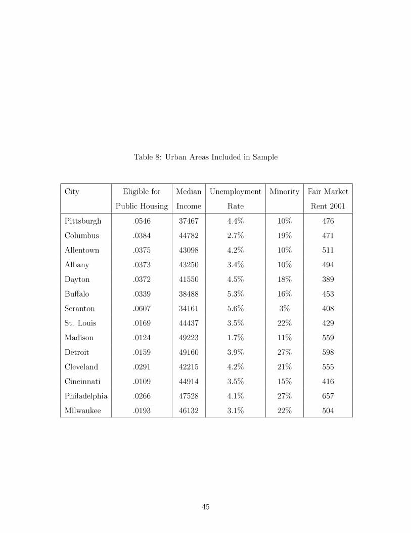
Table 8: Urban Areas Included in Sample

City Eligible for Median Unemployment Minority Fair Market

Public Housing Income Rate Rent 2001

Pittsburgh .0546 37467 4.4% 10% 476

Columbus .0384 44782 2.7% 19% 471

Allentown .0375 43098 4.2% 10% 511

Albany .0373 43250 3.4% 10% 494

Dayton .0372 41550 4.5% 18% 389

Buffalo .0339 38488 5.3% 16% 453

Scranton .0607 34161 5.6% 3% 408

St. Louis .0169 44437 3.5% 22% 429

Madison .0124 49223 1.7% 11% 559

Detroit .0159 49160 3.9% 27% 598

Cleveland .0291 42215 4.2% 21% 555

Cincinnati .0109 44914 3.5% 15% 416

Philadelphia .0266 47528 4.1% 27% 657

Milwaukee .0193 46132 3.1% 22% 504

45

for low-income households.

Table 9: Parameter Estimates

Full Sample Pitt SIPP Only

Income 0.329 (0.028) 0.327 (0.038)

Moving cost -3.186 (0.017) -3.203 (0.036)

Afr. Amer. and non-senior 1.222 (0.071) 1.221 (0.107)

White and senior 0.209 (0.113) 0.209 (0.152)

Afr. Amer. and senior 1.000 (0.101) 1.001 (0.138)

Children -0.315 (0.123) -0.317 (0.185)

Female 0.053 (0.061) 0.054 (0.090)

Female and senior -0.174 (0.094) -0.174 (0.121)

Female with children 0.426 (0.130) 0.424 (0.195)

community community

fixed effects fixed effects

Estimated standard errors are given in parenthesis.

A more formal sensitivity test is to compare estimates of the model obtained using

the full HACP and SIPP samples, to the estimates of the model obtained using full

HACP sample and only the SIPP samples from Pittsburgh. The results are reported

in Table 9. We find that the point estimates are very similar. Not surprisingly, the

estimated standard errors are larger when the SIPP sample is reduced to include only

observations in Pittsburgh. We conclude that the our estimates are not seriously

driven by the composition of our “control” sample.

46

C Ignoring the Supply Side Restrictions

Table 10 reports the estimates obtained from a logit demand model that ignores the

supply side restrictions and compares to our baseline estimates.

Table 10: Comparison with Simple Logit

Our Model Simple Logit

Income 0.329 (0.028) 0.436 (0.018)

Moving cost -3.186 (0.017) -5.512 (0.015)

Afr. Amer. and non-senior 1.222 (0.071) 1.775 (0.034)

White and senior 0.209 (0.113) 0.612 (0.043)

Afr. Amer. and senior 1.000 (0.101) 1.161 (0.042)

Children -0.315 (0.123) -0.766 (0.083)

Female 0.053 (0.061) 0.195 (0.035)

Female and senior -0.174 (0.094) -0.136 (0.043)

Female with children 0.426 (0.130) 0.479 (0.086)

PH1 4.217 (0.254) -0.6363 (0.158)

PH2 4.848 (0.261) -0.895 (0.165)

PH3 4.604 (0.277) -1.672 (0.170)

PH4 4.394 (0.260) 0.101 (0.163)

PH5 4.626 (0.263) -1.538 (0.158)

PH6 4.907 (0.258) -0.837 (0.154)

log likelihood -688,796 -653,936

Estimated standard errors are given in parenthesis.

47