Estimates of global biomass burning emissions for reactive

Estimates of global biomass burning emissions for

reactive greenhouse gases (CO, NMHCs, and NOx) and CO2

Atul K. Jain,1 Zhining Tao,1 Xiaojuan Yang,1 and Conor Gillespie1

Received 18 May 2005; revised 26 October 2005; accepted 2 December 2005; published 22 March 2006.

[1] Open fire biomass burning and domestic biofuel burning (e.g., cooking, heating, andcharcoal making) algorithms have been incorporated into a terrestrial ecosystem model toestimate CO2 and key reactive GHGs (CO, NOx, and NMHCs) emissions for the year2000. The emissions are calculated over the globe at a 0.5� � 0.5� spatial resolutionusing tree density imagery, and two separate sets of data each for global area burned andland clearing for croplands, along with biofuel consumption rate data. The estimatedglobal and annual total dry matter (DM) burned due to open fire biomass burning rangesbetween 5221 and 7346 Tg DM/yr, whereas the resultant emissions ranges are 6564–9093 Tg CO2/yr, 438–568 Tg CO/yr, 11–16 TgNOx/yr (as NO), and 29–40 TgNMHCs/yr.The results indicate that land use changes for cropland is one of the major sources ofbiomass burning, which amounts to 25–27% (CO2), 25 –28% (CO), 20–23% (NO), and28–30% (NMHCs) of the total open fire biomass burning emissions of these gases.Estimated DM burned associated with domestic biofuel burning is 3,114 Tg DM/yr, andresultant emissions are 4825 Tg CO2/yr, 243 Tg CO/yr, 3 Tg NOx/yr, and 23 Tg NMHCs/yr.Total emissions from biomass burning are highest in tropical regions (Asia, America, andAfrica), where we identify important contributions from primary forest cutting forcroplands and domestic biofuel burning.

Citation: Jain, A. K., Z. Tao, X. Yang, and C. Gillespie (2006), Estimates of global biomass burning emissions for reactive

greenhouse gases (CO, NMHCs, and NOx) and CO2, J. Geophys. Res., 111, D06304, doi:10.1029/2005JD006237.

1. Introduction

[2] Assessing the impact of human activities on climatechange requires not only accurate emission estimates ofmajor greenhouse gases (GHGs) (e.g., carbon dioxide(CO2), methane (CH4), and ozone (O3)) but also emissionestimates of reactive GHGs (e.g., carbon monoxide (CO),nitric oxides (NOx), and nonmethane hydrocarbon com-pounds (NMHCs)). Reactive GHGs, although largely trans-parent to IR radiation, can impact the climate system byaltering the concentrations of CH4 and tropospheric O3 (twomajor GHGs) through complex chemical processes [Pratheret al., 2001]. A number of studies have emphasized theinteractive nature of CH4 and reactive GHGs, and theeffects these interactions can have on overall climate change[Fuglestvedt et al., 1996; Daniel and Solomon, 1998;Kheshgi and Jain, 1999; Kheshgi et al., 1999; Hayhoe etal., 2000].[3] Although energy related reactive GHG emissions are

relatively well represented in the current emission inventory,uncertainties in emissions from nonenergy sources (e.g.,biomass burning, vegetation, soil, ocean, and nonvehiclemobile sources) at the global level are considerably large[Prather et al., 2001]. In particular, biomass burning has

been identified as an important source of reactive GHGssince the early 1980s [Andreae and Merlet, 2001]. It alsoplays a central role in carbon cycling through the directrelease of CO2, the single most important anthropogenicGHG, into the atmosphere during biomass burning. At thesame time, studies also suggest that fire and loggingincreases the vulnerability of forests to future burning[Cochrane et al., 1999; Keeley et al., 1999; Nepstad etal., 1999]. Because of the impact that reactive GHGemissions from biomass burning exert on atmosphericchemistry and the carbon cycle, the development of acomplete emission inventory is vital to the successful studyof global atmospheric chemistry and climate change.[4] Earlier global modeling estimates of biomass burning

emission inventories relied on scattered and incomplete dataof available fuel for burning and the percentage of fuel thatis actually burned over a specific time period [Crutzen andAndreae, 1990; Hao et al., 1990; Hao and Liu, 1994; Lobertet al., 1999; Galanter et al., 2000]. The uncertainties ofthese inventories are considerably high. More recently, themodeling studies have taken advantage of available satelliteremote sensing data and/or more comprehensive biogeo-chemical models to estimate the amount of biomass burnedowing to open fire and associated emissions [van der Werfet al., 2003, 2004; Ito and Penner, 2004; Hoelzemann et al.,2004].[5] The purpose of this study is to build upon and extend

the approaches of previous studies. While we use the sameor similar information for combustion completeness and

JOURNAL OF GEOPHYSICAL RESEARCH, VOL. 111, D06304, doi:10.1029/2005JD006237, 2006

1Department of Atmospheric Science, University of Illinois, Urbana,Illinois, USA.

Copyright 2006 by the American Geophysical Union.0148-0227/06/2005JD006237$09.00

D06304 1 of 14

emission factors, we implement these data in our newlydeveloped independent ISAM (Integrated Science Assess-ment Model) terrestrial ecosystem model to estimate theemissions of reactive GHGs from open fire biomass burningand domestic biofuel burning (e.g., cooking, heating, andcharcoal making). The advantage of implementing the bio-mass emission relationship into the ISAM terrestrial ecosys-tem model is that we can account for the aboveground andsurface fuel removed by land use changes. Although sucheffects have generally been implicitly calculated in recentmodeling studies of biomass burning [van der Werf et al.,2003, 2004; Ito and Penner, 2004;Hoelzemann et al., 2004],the land use component has not been systematically deter-mined. This approach includes the influence on fuel load ofvarious ecosystem processes (such as stomatal conductance,evapotranspiration, plant photosynthesis and respiration,litter production, and soil organic carbon decomposition)and important feedback mechanisms (such as the climateand fertilization feedback mechanisms). In this paper, theISAM terrestrial ecosystem model, along with availabledata sets for the global area burnt, land use changes, andforest density, have been used to study the global emissionsfor reactive greenhouse gases (CO, VOCs, and NOx) andCO2 emissions in the year 2000. The results are comparedwith other recently published model results and data-basedstudies that use similar data sets and modeling approaches.Finally, the sources of uncertainties in various input param-eters and model results, and the potential for reduction ofthese uncertainties are discussed.

2. Methodology

[6] The emission calculations associated with open firesand land clearing for croplands were carried out using thestandard method for estimating emissions from biomassburning [Seiler and Crutzen, 1980; Hao et al., 1990;Pereira et al., 1999; Potter et al., 2002]. According to thismethod the total yearly emissions (Eij, Tg/yr) of a gas forvegetation type i within a grid cell j are

Eij ¼ DM½ �ij � CC½ �ij � EF½ �ij;

DMij ¼X12t¼1

A½ �ijt � AFL½ �ijt� �

for nonclearing for cropland fires;

DMij ¼ A½ �ij � B½ �ij � a½ �ij for clearing for cropland fires;

where DM is the dry matter burned (kg) for vegetation type iwithin each grid cell j, CC is the combustion completenessor efficiency for vegetation type i within each grid cell j, andEF (g species/kg dry matter) is an emission factor of a gasfor an open fire in ecosystem type i of grid cell j, t is thetotal number of months (t = 12), A (km2) is the total burntarea or cleared area (km2) for croplands for each vegetationtype i within each grid cell j, AFL (kg dry matter/km2) is themonthly available fuel load or burnable plant material forvegetation type i within each grid cell j, B (kg/km2) is thebiomass cleared for croplands for vegetation type i withineach grid cell j. a is the fractions of total cleared vegetation

burned for vegetation type i within each grid cell j. CC andEF considered in this study are also functions of vegetationtype and region. The global and annual emissions for CO,NMHCs, and NOx (as NO) are calculated at 0.5� � 0.5�spatial resolution. B and AFL are calculated using theterrestrial component of the ISAM coupled with the latestforest canopy cover density map produced from theAVHRR 1 km resolution satellite data set [Zhu and Waller,2003]. In order to obtain regional information about thebiomass burning related emissions we divided the globalland into nine regions, depicted in Figure 1.

2.1. Available Fuel Load

[7] In this study, the global biomass density to determineavailable fuel load (AFL) or pre-burnable plant material iscalculated using the terrestrial component of our ISAM[Jain and Yang, 2005]. The model simulates the carbonfluxes to and from different compartments of the terrestrialbiosphere with 0.5� � 0.5� spatial resolution. Each grid cellis occupied by at least one of the twelve natural landcoverage classifications and/or croplands (for example, agrid cell can contain 50% forest, 30% cropland and 20%grassland) according to the vegetation maps of Lovelandand Belward [1997] and Haxeltine and Prentice [1996], andby at least one of the 105 soil types based on the FAO-UNESCO Soil Map of the World [Zobler, 1986, 1999]representing both highly managed and less managed landcover types. We have considered only 10 natural vegetationtypes and croplands (Table 1). The two other vegetationtypes, tundra and polar desert, were omitted owing to theirinsignificance in estimating biomass burning activities.Within each grid cell, the carbon dynamics of each land-coverage classification are described by an ecosystemmodel consisting of ground vegetation (GV) representingherbaceous carbon reservoirs; nonwoody tree part (NWT)

Figure 1. Geographical distributions of the nine regionsconsidered in this study for the regional biomass burningemission analysis.

D06304 JAIN ET AL.: BIOMASS AND BIOFUEL BURNING EMISSIONS

2 of 14

D06304

representing foliage, flowers and roots in transition; woodytree parts (WT) representing branches, boles, and most rootmaterial of trees; two litter reservoirs (DPM and RPM,described below), representing litter input from above andbelow ground litter biomass plant parts; and three soilreservoirs (microbial biomass (BIO), humified organic mat-ter (HUM), and inert organic matter (IOM)). The ISAMterrestrial model also consists of forest clearing and agri-culture waste reservoirs. The carbon stored in these reser-voirs is released to the atmosphere at a variety of ratesdepending on usage and is assigned products into threegeneral reservoirs with turnover time of 1 year (agricultureand agriculture products), 10 years (paper and paper prod-ucts), and 100 years (lumber and long-lived products).[8] There are many features of this model that make it

suitable for estimating fuel loads. First, the separationbetween ground vegetation (GV) and two tree parts(NWT and WT) allow us to account for the distinct woodyand nonwoody biomass variation within each ecosystemtype.[9] Second, distinction between two kinetically defined

pools of plant litter, metabolic or decomposable (DPM) andstructural or resistant plant material (RPM), allows us toproperly account for partially decomposed organic materialfuel in the upper portion of the ground surface vegetation.Note that the DPM constitutes the cytoplastic compounds ofplant cells and is more susceptible to fires, whereas theRPM represents the cell wall with bound protein andlignified structures and is less susceptible to fires thanDPM plant material.[10] Third, the forest clearing and agriculture waste

reservoirs allow us to account for biomass burned throughland transformation. Studies suggest that models may beunderestimating the total biomass burning emissions owingto omission of these effects [Scholes et al., 1996].[11] Finally, the ISAM modeling approach allows us to

estimate the time dependent AFL. Owing to the longturnover times of some of the model reservoirs, the carbonis accumulated over many years to generate the biomass in

different terrestrial ecosystem reservoirs. Therefore we firstinitialized the vegetation model with a 1765 atmosphericCO2 concentration of 278 ppmv to calculate the equilibriumnet primary production (NPP) in addition to vegetation andsoil carbon for different model pools. Next, we ran themodel at a monthly time step up to the year 2000 usingobserved monthly temperature and precipitation changes(T. D. Mitchell et al., A comprehensive set of high-resolutiongrids of monthly climate for Europe and the globe: Theobserved record (1901–2000) and 16 scenarios (2001–2100), submitted to Journal of Climate, 2005) and CO2

concentrations [Neftel et al., 1985; Friedli et al., 1986;Keeling and Whorf, 2000]. We also utilized surveys of pastland cover changes due to three types of land cover changeactivities: clearing of natural ecosystems for croplands and/or pasturelands, recovery of abandoned croplands/pasture-lands to preconversion natural vegetation, and productionand harvest in conversion areas [Jain and Yang, 2005].[12] In order to account for fire in the ISAM, two

modifications were implemented. First, we assume that onlysurface and aboveground biomass is accessible for burning(i.e., excluding live and dead root material). Part of theabove ground dead biomass, such as fine leaf and grass, isentered into the DPM pool and assumed to decay metabol-ically. The rest of the above ground dead biomass, such asbranches and heavy lignified material, enters the RPM pooland is assumed to structurally decompose. The DPM andRPM also contain the belowground dead fine and heavyroots, which are assumed not to be part of the biomassdensity susceptible to burning. The different resolutions ofthe two burned data sets (1 km � 1 km) and the ISAMterrestrial model (0.5� � 0.5�) needed to be integrated, inorder to account for spatial variability in forest and non forestbiomass at 0.5� � 0.5� resolution. To do this we estimate thefraction of forest and nonforest plant material area withineach burned 1-km grid cell using the latest forest canopycover density map produced from the global forest cover mapof the USGS (U.S. Geological Survey) [Loveland et al.,1999], in combination with the AVHHR 1-km data forgeographical distribution and conditions of global forestresources [Zhu and Waller, 2003]. Next, we sum all forestand nonforest burned plant material area within each 0.5� �0.5� grid cell. Then we multiply these areas (in m2) by thecorresponding half-degree model-determined burned treeand nontree biomass density (in gC/m2). The nontree burneddensity is assigned to herbaceous plants represented by theGV pool, whereas the tree burned biomass density isassigned to the WT and NWT pools.[13] Using Zhu and Waller’s [2003] fractional tree cover

map, the global and annual tree-covered burned areadetected by the GLOBSCAR and GBA (discussed insection 2.4) products were 442,435 km2 and 747,000 km2,respectively. At the same time, GLOBSCAR and GBAproducts reported global total forest area burned of307,000 km2 [Simon et al., 2004], and 700,000 km2 [Tanseyet al., 2004], respectively. Our estimated values for theGLOBSCAR and GBA data are slightly higher than Simonet al. [2004] and Tansey et al. [2004], respectively, asdiscussed in section 3.2.[14] The total preburnt accessible vegetation carbon den-

sity for each grid cell is the sum of vegetation density ofGV, WT (branches and boles), NWT, DPM, and RPM.

Table 1. Percentage of Accessible Carbon Vegetation Density

(ACVD) Susceptible for Burning for Each Ecosystem Type and

Carbon Pool

Land Cover Type GV NWT WT DPM/RPMa

Tropical evergreen 50b 50b 20c 100/30Tropical deciduousd 60 60 24 100/30Temperate evergreen 50e 10c 10c 100/30Temperate deciduousd 60 12 12 100/30Boreal 50e 25c 25c 100/30Savanna 98f 0g 0g 100/0Grassland 98f 0g 0g 100/0Pastureland 58f 0g 0g 100/0Shrubland 98f 0g 0g 100/0Cropland 98f 0g 0g 100/0

aAssume 100% of the accessible biomass of the DPM litter pool isavailable for burning, while only 30% and 0% of the accessible biomass ofRPM is available for burning in forest and nonforests regions, respectively.

bGoldammer and Mutch [2001].cHoelzemann et al. [2004].dAssume 20% higher than evergreen forests.eSoja et al. [2004].fShea et al. [1996].gShea et al. [1996]; Hoffa et al. [1999]; Scholes et al. [1996].


3 of 14

D06304

Subsequently, the total biomass fuel density from totalcarbon density is converted by assuming 45% carbon perunit of total biomass for all natural vegetation types andcroplands [Scholes and Walker, 1993].[15] Not all of the ISAM estimated accessible vegetation

carbon density (g/m2) (AVCD) is subject to biomass burn-ing. The amount (in%) of AVCD per ecosystem and carbonpool that is available for burning depends mainly on theseverity of the fire [Hely et al., 2003; Lambin et al., 2003;Soja et al., 2004]. On a forest stand scale, severity is relatedto the fire type (i.e., surface or crown), fire intensity, specificforest ecosystem, and weather conditions. Since the twoburned data products used in this study only provide theinformation of the burned area occurrence in terms of‘‘0’’ (no biomass burning) or ‘‘1’’ (biomass burning) ineach 1-km area, rather than the type of fire for area burnt,we are forced to estimate the percentage of AVCD suscep-tible for burning according to the literature where availableand according to our best judgment where necessary. Owingto this limitation with the area burned data, we also do notaccount for the fire-induced mortality of living biomass.Table 1 provides the percentage of AVCD susceptible forburning for each ecosystem type and carbon pool. Finally,AFL is calculated by multiplying the model estimatedAVCD by the percentage values given in Table 1.

2.2. Combustion Completeness

[16] Combustion completeness (CC), also called com-bustion fraction, is highly variable between different firesunder different conditions even in similar vegetation types.However, CC for different ecosystem types can be looselyassociated with fuel types, fuel loads, fuel configurations,and resulting combustion processes associated with thoseecosystems. In this study, ecosystem types with similarcharacteristics are grouped together and assigned a CCbased on the literature survey (Table 2). In some cases, wehave used the averaged values for some of the ecosystemtypes because there are various field study results avail-able for the same ecosystem type in the open literature,which give different numbers for CC. In the absence ofthe existence of a rigorous approach, we average thevalues for the different studies to give a representativevalue of CC.

2.3. Emission Factors

[17] Emission factors (EFs) are estimations of the mass ofa given species emission relative to some measurement oftotal burned material. In this study, all EFs are given interms of g species/kg dry matter. We use regional natural

vegetation-based EFs (listed in Table 3), which are com-piled from several publications for various regions andecosystems. If the EF of a gas is available from manydifferent sources, we use the average value of all availablesources. In addition, if there is no regional EF valueavailable, a global mean EF derived by Andreae and Merlet[2001] for different natural vegetation type is used.

2.4. GLOBSCAR and GBA Burnt Area Data Sets

[18] For the global burnt area we have used two of thelatest open fire products recently made available. Bothproducts are compilations of global monthly area burnedduring the year 2000 from two different remote sensingsatellites. These two data sets are GLOBSCAR [Simon etal., 2004] and GBA [Gregoire et al., 2003; Tansey et al.,2004]. Both data sets are freely distributed products andprovide the monthly areas burned globally at 1 km � 1 kmresolution.[19] Both data sets have a number of shortcomings with

respect to global biomass emission calculations. One ofthe common problems associated with both data sets isthat they do not detect small burnt areas below 1 km2.Previous emission inventory studies based on GLOBSCAR[Hoelzemann et al., 2004], and GBA [Ito and Penner, 2004]data sets have used the ATSR active fire counts [Arino andPlummer, 2001] to account for small-undetected burnt area.These studies found very small increases (1–2%) in the areaburned due to this correction [Ito and Penner, 2004;Hoelzemann et al., 2004]. Moreover, earlier studies havealso shown that the active fire products do not represent anunbiased sample of fire activity owing to poor samplingfrequency and failure to detect small daytime fires [Arinoand Plummer, 2001; Schultz, 2002; Kasischke et al., 2003].Therefore we do not apply this active fire count datacorrection in the current study.[20] Two satellite data sets may also detect nonbiomass

fires such as oil/gas flares and coal-mine fires. In this study,we prevent such problem by adding an algorithm in ourcalculation such that if burning occurs in the same pixel forfour continuous months, we regard that burning as oil/gasflares or coal-mine fires and remove it from the calculationof total biomass burning emissions.[21] The annual global burned areas used in this study for

the year 2000 based on GLOBSCAR and GBA data setswere about 1.92 million km2 and 3.49 million km2, whichare slightly lower than the area burned originally reportedby the authors of GLOBSCAR (2.10 million km2) [Simon etal., 2004] and GBA (3.52 million km2) [Tansey et al., 2004]data sets, because we have excluded tundra and polar desert

Table 2. Combustion Completeness (CC) for Different Land Cover Types

Land Cover Type Combustion Completeness, % Source

Tropical evergreen 0.50 Fearnside [2000]Tropical deciduous 0.50 Fearnside [2000]Temperate evergreen 0.50 Hoelzemann et al. [2004]Temperate deciduous 0.50 Hoelzemann et al. [2004]Boreal 0.50 Hoelzemann et al. [2004]Savanna 0.75 Average of Ward et al. [1996], Hoffa et al. [1999],

and Hely et al. [2003]Grassland/Pastureland 0.83 Average of Hoffa et al. [1999] and Fearnside [2000]Shrubland 0.75 Average of Ward et al. [1996], Hoffa et al. [1999],

and Hely et al. [2003]Cropland 0.86 Saarnak et al. [2003]


4 of 14

D06304

from burning owing to their negligible contributions inestimating biomass burning activities. As demonstrated byFigures 2a and 2b, the GBA results for most regions aresubstantially higher than GLOBSCAR results. This issuehas been investigated in some detail by Simon et al. [2004],who compared the GLOBSCAR results to available statis-tics and other remote sensing products including ATSR-2World Fire Atlas (WFA) [Arino et al., 2001] and the GBAresults; and by Tansey et al. [2004] who compared the GBAresults to the available national burned statistics and

GLOBSCAR results for several regions. These previouscomparisons help us to draw some conclusions about thepotential and limitations of the GLOBSCAR and GBAresults regionally. The most notable regional differencesbetween the two data sets are seen in tropical Africa andOceania, perhaps owing to known difficulties with GLOBS-CAR detection of woodland and shrubland burning [Simonet al., 2004]. The annual burnt area recorded by GLOBS-CAR in North America and tropical America is higher thanthat recorded by GBA. While the authors of the GBAproducts acknowledge underdetection problems over NorthAmerica, particularly in Canada [Tansey et al., 2004],Simon et al. [2004] assert that the GBA product may beoverreporting area burned owing to the mapping of scarsfrom previous fires. GLOBSCAR results for tropical Amer-ica are generally equal to what might be expected in thisregion [Simon et al., 2004]. In the case of Tropical Asia and

Table 3. Emission Factors for Different Land Cover Types and

Regions for Various Greenhouse Gas Emissionsa

CO NOx NMHCs CO2

Tropical EvergreenTropical America 122b 2.7c 8.4d 1580Other Regionse 104 1.6 8.1 1580

Tropical DeciduousTropical America 79.2f 3.4g 8.1 1580Other Regionse 104 3.0 8.1 1580

Temperate Evergreen and Temperate DeciduousNorth America 98.5h 3.0 5.7 1569Other Regionse 107.0 3.0 5.7 1569

BorealNorth America 115.0i 1.5j 5.7 1569Former Soviet Union 175.7k 3.0 5.7 1569Other Regionse 107 3.0 5.7 1569

SavannaTropical America 58.6l 2.3d 3.6d 1613Tropical Africa 67.0m 3.1n 2.9o 1613Oceanic 80p 1613Other Regionse 65.0 3.9 3.4 1613

Grassland/Pastureland/Shrubland/DesertTropical Africa 62.4q 5.5r 3.6s 1613Other Regionse 65.0 3.9 3.4 1613

CroplandTropical Africas 117.0 2.8 5.0 1515Other Regionse 92.0 2.5 7.0 1515

aEmission factors (EF), given in g species/kg dry matter.bAverage of Ferek et al. [1998], Fearnside [2000], and Scholes and

Andreae [2000].cAverage of Fearnside [2000] and Scholes and Andreae [2000].dScholes and Andreae [2000].eAndreae and Merlet [2001].fAverage ofWard et al. [1996], Bertschi et al. [2003], Sinha et al. [2003],

and Yokelson et al. [2003].gSinha et al. [2003].hAverage of Yokelson et al. [1999] and Friedli et al. [2001].iAverage of Cofer et al. [1989, 1998], Hegg et al. [1990], Radke et al.

[1991], Susott et al. [1991], Yokelson et al. [1997], Goode et al. [2000],Bertschi et al. [2003], and French et al. [2002].

jGoode et al. [2000].kAverage of Cofer et al. [1996] and Bertschi et al. [2003].lAverage of Ward et al. [1992] and Ferek et al. [1998].mAverage of Cofer et al. [1996], Hao et al. [1996], Scholes et al. [1996],

Sinha et al. [2003], and Yokelson et al. [2003].nAverage of Lacaux et al. [1996], Scholes et al. [1996], Sinha et al.

[2003], and Yokelson et al. [2003].oAverage of Cofer et al. [1996], Ward et al. [1996], Korontzi et al.

[2003], and Sinha et al. [2003].pHurst et al. [1994a, 1994b] and Shirai et al. [2003].qAverage of Scholes et al. [1996], Ward et al. [1996], Korontzi et al.

[2003], Sinha et al. [2003], and Yokelson et al. [2003].rScholes et al. [1996].sSaarnak et al. [2003].

Figure 2a. Regional area burned (million km2) from theopen fires in the year 2000 based on GLOBSCAR and GBAdata sets.

Figure 2b. Monthly area burned (million km2) from theopen fires for the year 2000 based on GLOBSCAR andGBA data sets.


5 of 14

D06304

China, the GLOBSCAR results for area burnt are about50% lower than the GBA results. Simon et al. [2004] reportthat there were no validation data available for theseregions. In Europe, North Africa, the Middle East, andthe Former Soviet Union, burnt area based on both datasets are approximately the same. However, in the case ofthe Former Soviet Union, both the GLOBSCAR figuresand GBA results are significantly larger than nationalreports and UN FAO statistics [Simon et al., 2004; Tanseyet al., 2004].

2.5. Emissions From Land Clearing for Croplands

[22] To calculate the burning emissions due to changes innatural vegetation for croplands, a specified amount ofbiomass within a grid cell is subtracted from the threevegetation carbon pools (GV, NW, WTP) based on therelative proportions of the carbon contained in thesereservoirs. A fraction of the released carbon is transferredto litter reservoirs as slash left on the ground. The rest isstored in burnable plant material pool (1-year pool) andwood and/or fuel product reservoirs (10-year, 100-yearpools). The values of the fractions of total cleared vegeta-tion burned (a), and used for wood and fuel products aretaken from Houghton and Hackler [2001], which varieswith land cover type and region. In order to avoid thedouble accounting of biomass burning due to land clearingdata and satellite-based burning data within each 0.5 and0.5 grid cell, the satellite data-based DM burned is revisedby subtracting the DM burned owing to land clearing forcroplands.[23] The DM burned owing to land clearing for croplands

is calculated on the basis of two sets of data for area clearedfrom croplands as implemented by Jain and Yang [2005].The first set of data is primarily based on the deforestationrates compiled from national reports and remote sensingsurveys from the United Nations FAO (Food and Agricul-ture Organization) Forest Resource Assessment (FRA)[Houghton, 2003; Houghton and Hackler, 1999, 2001](HH hereafter) The HH data is available over the period1765–2000. The other set of data is based on croplandstatistics from the United Nations FAO [Ramankutty andFoley, 1998, 1999] (RF hereafter). The RF data set isavailable for the period 1765–1992. In order to calculateDM in the year 2000, we linearly extrapolated the RF databetween 1992 and 2000 using the trend for the 1980s.

2.6. Emissions From Domestic Biofuel Burning

[24] Emissions from domestic biofuel burning in the year2000 were calculated by multiplying the per capita fuelconsumption rate by the total population. We use Ludwig etal.’s [2003] regional per capita consumption rates. The percapital domestic biofuel consumption rate covers all theactivities associated with biofuel burning (e.g., cooking,heating, and charcoal making). The gridded 1990s worldpopulation from the United Nations Environmental Program(http://esa.un.org/unpp/) was projected to the year 2000 onthe basis of the census population growth data from theUnited Nations. The estimated regional biofuel consump-tion was then distributed among the grids in each region bymultiplying the population density per grid with the con-sumption rate for that region. Most fuelwood used indomestic biofuel burning comes from local ecosystems; as

such, there is potential for errors due to double countingbiomass usage. Double counting occurs when all biomass ina grid is used in the biomass burning calculation, and thenfuelwood consumption of the same biomass occurs in thesame grid. The assumption made in this study was that allfuelwood burned in a grid came from the biomass in thesame grid. To minimize errors, fuelwood consumption wascalculated per grid and then a check was done to see ifburning occurred in that grid. If burning occurred within agrid cell, the biomass from fuelwood consumption wassubtracted from the burned biomass load. On the basis oftwo burnt area data sets, about 3–5% of the fuelwoodconsumption was subtracted.

3. Results

3.1. Available Fuel Load

[25] Table 4 compares our ISAM model estimated AFLfor various regions and across major ecosystem types withfield experiment–based values available in the literature. Itis important to recognize that there is no consistent globalmap of AFL available in the open literature. Most of thefield experiment studies available in the literature are carriedout on specific regions or a country using diverse methods.Therefore the uncertainty ranges for the available literaturevalues are generally quite large (Table 4). Results from thisstudy using tree density imagery as inputs to the terrestrialcomponent of our ISAM indicate that the global and annualtotal AFL in the year 2000 for forest and nonforest biomeswere 14,259 g/m2 and 1073 g/m2. The nonforest and forestbiomes account for 10 and 90% of the global total AFL(687 Pg AFL/yr). Our modeling results indicate that theFormer Soviet Union (FSU) forests contain the largestamount of AFL on the basis of density (18 kg/m2), thenNorth America (NA) (16 kg/m2), North Africa and theMiddle East (NAME)(15 kg/m2), Tropical Africa (TAf)(13 kg/m2), Tropical America (Tam) and Europe (EU)(12 kg/m2), and Tropical Asia (TAs) (11 kg/m2). All otherregions produced less than 10 kg/m2 AFL from forestbiomes. In the case of nonforests, again FSU biomes containthe largest amount of AFL (1.9 kg/m2), then EU (1.8 kg/m2),TAs (1.4 kg/m2) and, NA and China (1.0 kg/m2); whereasother regions contain less than 1.0 kg/m2n of nonforest AFL.

3.2. Dry Matter Burned

[26] Table 5 lists the ISAM estimated regional and totalestimated global and annual mean dry matter (DM) burned(Tg DM/yr) based on various data sets for open fire biomassand domestic biofuel burning. The ISAM estimated drymatter burned, without land clearing for croplands, based onGLOBSCAR and GBA data sets for the year 2000 were3099 Tg DM/yr and 4159 Tg DM/yr (Table 5). The differ-ences in estimated DM burned for two data sets are due notonly to the differences in the area burned, but also to thedifferences in fuel type burned (forests versus nonforest)from the two data sets described in section 2.4. On the basisof these two data sets, the TAf (1712–2654 TgDM/yr) regionwas the largest source of DM burned. The FSU was thesecond largest source of DM burned (586–670 Tg DM/yr).The estimated DM burned in the year 2000 for other regionswere less than 500 Tg DM/yr (shown in Table 5). Our modelestimated results are consistent with other modeling studies


6 of 14

D06304

except for a few cases. For example, the ISAM estimatedDM burned based on of GLOBSCAR and GBA data sets formost regions were substantially lower than van der Werf etal. [2003], which were averaged over the period 1998–2001. It is important to point out here that 1998 was an ElNino year with increased fire activity due to droughtconditions, whereas the year 2000 was a La Nina year withless fire activity around the globe [van der Werf et al.,2003]. This could be one of the reasons that the area burnedestimates based on work by van der Werf et al. [2003],particularly in the tropics with the exception of the TAf forthe GBA case, were higher than the ISAM estimates basedon both (GBA and GLOBSCAR) data sets. The differencesbetween the estimated DM of the ISAM and other studiesmight also be due to the differences in the AFL and CCvalues for different vegetation types, as well as differentsatellite platforms and different years of burning data sets.These other factors could be the reasons that the DM burnedbased on van der Werf et al. [2003] in TAf were lower thanthe ISAM estimates based on GBA data set, whereas theestimates were higher than the ISAM estimates based onGLOBSCAR. Andreae and Merlet [2001] also provided theglobal total value of DM burned for the late 1990s (5130 TgDM/yr), which was originally estimated by J. A. Logan andR. Yevich from statistical ground-based measurement assummarized by Lobert et al. [1999]. The Andreae andMerlet [2001] value was higher than our estimated rangeof values (3099–4159 Tg DM/yr).[27] Our modeling results suggest that land clearing for

croplands in the year 2000 was the primary source of DMburned. The ISAM estimated total biomass burned based ontwo sets of satellite data for area burned (GLOBSCARand GBA) and land clearing data (RF and HH) were 5221–

7346 Tg DM/yr. The land clearing for cropland sourcecontributed 2122–3187 Tg DM/yr (39 to 44% of total).The DM based on the RF data set was about 35% lower thanthat based on the HH data sets, mainly because the landclearing rates based on RF were lower than HH, particularlyin the TAf. In general, our model results show the largestDM burned due to land clearing in tropical regions: TAs(1633–1925 Tg DM/yr), TAf (58–1013 Tg DM/yr), andTAm (99–201 TgDM/yr) (see Table 5). The data indicatethat the land clearing activities were negligible in thenontropical regions. Therefore the estimated DM burnedin these regions was either zero or small (Table 5).[28] The estimated total annual and global DM burned

due to domestic biofuel burning for the year 2000 was3114 Tg DM/yr representing approximately 40–60% of thetotal DM burned due to biomass burning (see Table 5). Ourestimates of DM burned due to domestic biofuel burningwere higher than the estimates of Andreae and Merlet[2001], who reported 2701 Tg DM/yr. On the regionalscale, the largest biofuel consumption occurred in TAs(940 Tg DM/yr), China (686 Tg DM/yr), and TAf (559 TgDM/yr). Our estimated domestic biofuel DM burned forthese regions were consistent with recent estimates byYevich and Logan [2003].

3.3. Emissions From Open Fire Biomass and DomesticBiofuel Burning

3.3.1. Annual Global Total Emissions[29] Our model estimated reactive GHG and CO2 emis-

sions for the year 2000 from open fire biomass anddomestic biofuel burning sources are summarized inTable 6. Overall, our modeled global total emissions dueto biomass burning for the 2000 were 438–568 Tg CO/yr,

Table 4. ISAM Estimated Available Fuel Load for Forest Ecosystems as Well as Totals for Forest and Nonforests Ecosystems and

Regions for the Year 2000 Compared With Estimates Based on Field Measurementsa

Region Tropical Temperate Boreal Total for Forest Ecosystem Total for Nonforest Ecosystem

Tropical America 11,277 13,586 n/a 12,297 60012,000–43,000b 710d

6400–43,500c

Tropical Africa 12,740 9800 n/a 12,738 7569400–45,700e 72–478f

Tropical Asia 11,061 n/a n/a 11,061 1370North America n/a 14,257 16,803 16,245 1037

10,000–38,000g 8700–22,900h

19,200i

Europe 18,333 12,371 10,819 11,520 1837Former Soviet Union n/a 14,054 18,347 18,018 1910

5000j

North Africa and Middle East n/a 15,744 n/a 15,744 491China 12,096 8172 7302 8109 1013Oceania 11,471 11,941 n/a 11,766 653Global total 12,189 12,799 16,379 14,259 1073aAvailable fuel load in units of g/m2.bBrazil [Ward et al., 1992; Kauffman et al., 1995; Guild et al., 1998].cBrazil [Stocks and Kauffman, 1997].dBrazilian savanna and grassland [Ward et al., 1992; Guild et al., 1998].eRange values based on Guinean and Sudanian Savanna [Pereira et al., 1999].fSouth African and Zambian Savanna and Grassland [Shea et al., 1996].gRange values based on Oregon and Washington, U.S. regions [Hobbs et al., 1996].hRange values for Alaska Boreal regions taken from Kasischke et al. [2000]. The values were given in tC/ha, which were converted into total biomass by

assuming 45% carbon per unit of total biomass.iSurface biomass value for Alaska Boreal Forest taken from Apps et al. [1993].jSiberia, Russia [FIRESCAN Science Team, 1996].


7 of 14

D06304

11–16 Tg NOx/yr (as NO), 29–40 Tg NMHCs/yr, and6564–9093 Tg CO2/yr; whereas other modeling study esti-mates ranged between 171– –429 Tg CO, 16–24 Tg NOx

(as NO), 9–29 Tg NMHCs and 4477–7864 Tg CO2

[Andreae and Merlet, 2001; Duncan et al., 2003; Ito andPenner, 2004; van der Werf et al., 2003, 2004; Hoelzemannet al., 2004]. It is important to note that our model estimatedvalues for most of the cases are higher than those estimated

Table 5. Comparison of the Estimated Dry Matter Burned for the Year 2000 With Other Model-Based Studiesa

Region

Open Fire Biomass BurningDomestic Biofuel

Burning

Without Land Clearing Land Clearing TotalISAM ISAM-Biofuel

OtherStudiesISAM-GLOBSCAR ISAM- GBA Other Studies ISAM- RF ISAM- HH

Tropical America 181 145 177–187b 99 201 244–382 231 328e

1510c 1570d 120d

Tropical Africa 1712 2654 1824–2705b 58 1013 1770–3667 559 536e

2170c 704–2168f 180d

2320d

Tropical Asia 88 148 124–143b 1633 1925 1721–2073 940 930e

770c 880d 320d

North America 405 164 840c 47 0 164–452 231Europe 24 28 48 0 28–72 76Former Soviet Union 586 670 159 0 586–829 96North Africa and Middle East 12 9 28 7 16–40 255China 39 138 42 0 39–180 686 677e

Oceania 51 201 340c 8 40 59–241 39 1d

208–287b 319d

Global total 3099 4159 5630c 2122 3187 5221–7346 3114 2701g

2794–3814b

5130g

aDry matter burned in units of Tg DM/yr.bYear 2000 using the GBA global area burned data [Ito and Penner, 2004].cAverage for the period 1998–2001 using the TRMM satellite data for the region between 38�N and 38�S [van der Werf et al., 2003].dFor late 1970s [Hao and Liu, 1994].eYear 1995 derived from statistical ground-based estimates [Yevich and Logan, 2003].fDuring 1985–1991 [Barbosa et al., 1999].gLate 1990s [Andreae and Merlet, 2001].

Table 6. Comparison of ISAM Estimated Open Fire Biomass and Domestic Biofuel Burning Emissions for CO,

NOx (as NO), NMHCs, and CO2 for the Year 2000 With Other Model-Based Emission Estimatesa

CO NOx NMHCs CO2

ISAM-Biomass BurningThis study: without landclearing (GLOBSCAR – GBA)

320.6–406.7 8.5–12.2 21.1–27.8 4888–6570

This study: land clearing (RF – HH) 112.1–163.0 2.2–3.6 8.1–12.1 1676–2523This study total 437.7–567.7 10.7–15.8 29.2–39.9 6564–9093b

Other studiesAndreae and Merlet [2001]c 423.4 16.5 29.4 7864Ito and Penner [2004]d 263.0–421.0 18.7–27.1 4477–5982van der Werf et al. [2003]e 7634Hoelzemann et al. [2004]f 271 24.3 8.8 5716van der Werf et al. [2004]g 171–408Duncan et al. [2003]h 429

Biofuel BurningThis study 242.8 3.4 22.7 4825b

Other studiesAndreae and Merlet [2001]c 209 2.9 19.6 4187Ito and Penner [2004]d 232 2.2 19.3 3853Yevich and Logan [2003]i 156 4.0 2688aEmissions are in units of Tg Gas/yr. Open fire biomass burning emissions are calculated on the basis of GLOBSCAR and

GBA fires, and HH and RF land clearing for cropland data sets, whereas domestic biofuel burning emissions are calculated onthe basis of the regional per capita biofuel consumption rates.

bThe total carbon lost from cropland clearing and biofuels (6501–7348 TgCO2/yr) is reasonably close to Houghton’s [2003]estimate of the amount of carbon released as a result of all clearing practices + fuelwood use (TgCO2/yr for the 1990s) (R. A.Houghton, personal communication, 2005).

cLate 1990s use global biomass burning inventory estimates. Emissions from charcoal are excluded.dYear 2000 uses global GBA burned data.eAverage for the period 1998–2001 uses the satellite TRMM data between 38�N and 38�S.fYear 2000 uses global GLOBSCAR open fire burned data.gYear 2000 uses the satellite TRMM data and an inverse analysis of atmospheric CO anomalies between 38�N and 38�S.hYear 1999 uses global ATSR and AVHRR fire-count data.iYear 1995 is derived from statistical ground-based estimates.


8 of 14

D06304

by other studies. However, our results without land clear-ing effects are in much better agreement with othermodeling results. These results clearly suggest that landclearing has a substantial influence on the emissions ofvarious tracers studied here. On the basis of our modelresults, the land clearing source constituted about 25–28%(CO), 20–23% (NO), 28–30% (NMHCs), and 25–27%(CO2) of the total open fire biomass burning emissions ofthese gases.[30] Figure 3 and Table 6 show the model estimated

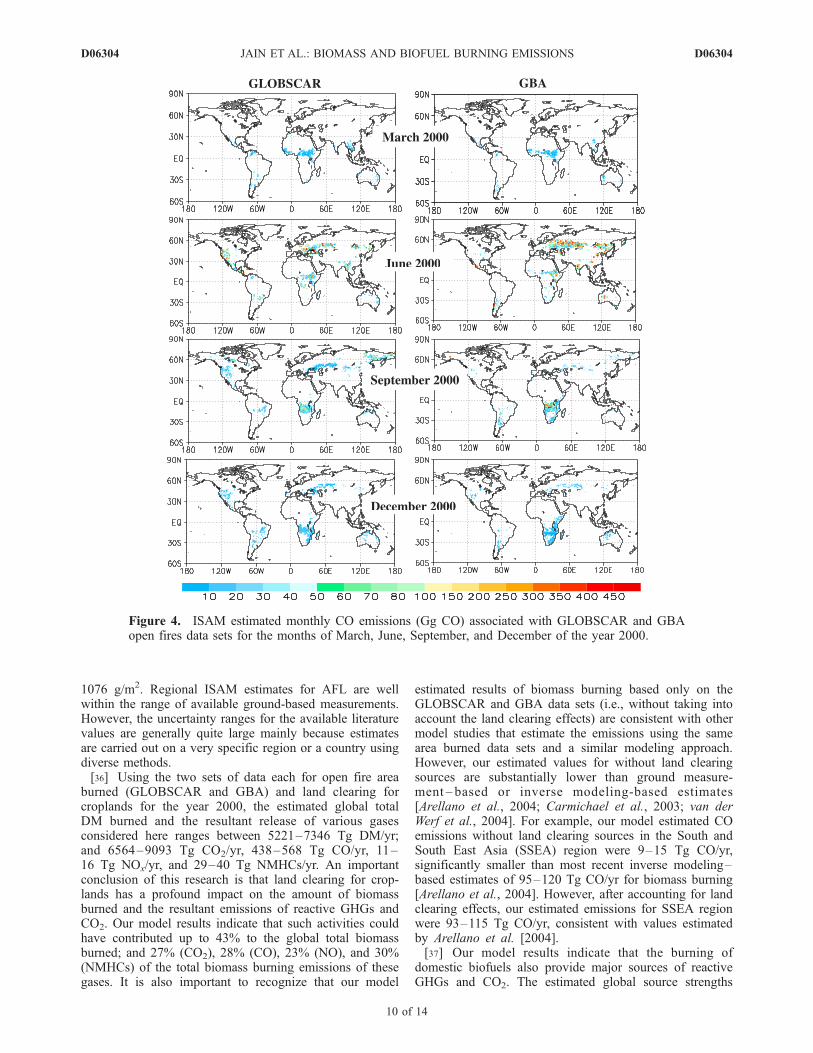
global distribution of CO emissions for the domestic biofuelburning in the year 2000. Our model estimated global ratesof 243 Tg CO/yr, 3 Tg NOx/yr (as NO), 23 Tg NMHCs/yr,and 4825 Tg CO2/yr were consistent with those of Andreaeand Merlet [2001] and Ito and Penner [2004]. Yevich andLogan [2003] estimated domestic biofuel emissions of156 Tg CO, 4.0 Tg NOx (as NO) and 2688 Tg CO2 forthe developing world (tropical Asia, tropical America,tropical Africa, and China). As compared to Yevich andLogan [2003], our model estimated emissions for thedeveloping world are somewhat higher in the case of CO(188 Tg CO) and CO2 (3745 Tg CO2), but lower in the caseof NOx (2.7 Tg NO).3.3.2. Spatial and Seasonal Distributions for Open FireEmissions[31] Spatial distributions of biomass-burning emissions

are exclusively tied to spatial detections of burned area byGLOBSCAR and GBA data sets. Large emissions occur inareas where heavy burning happens. This feature is wellillustrated in Figure 4, which displays the spatial distribu-tions of CO emissions associated with two fire data sets forthe months of March, June, September, and December ofthe year 2000 at 0.5� � 0.5� spatial resolution. The emissionestimates based on two burned products show roughlysimilar seasonal distributions throughout the year, but theirextent is lower in most of the regions when using theGLOBSCAR data set. All of these differences are furtherdiscussed below by comparing seasonal variations in COemissions for global total and nine regions based on twoarea burned data sets (Figure 5).

[32] It is important to recognize that the seasonal patternsof global total emissions for the CO based on two data setsare approximately the same, except for the month of Junewhen the emissions based on GBA data were decreasing,whereas emissions based on GLOBSCAR were rapidlypeaking. The most notable seasonal differences in COemissions based on two burned area products exist in NorthAmerica with much larger emission estimates based onGLOBSCAR in the month of June of 2000 than emissionestimates based on GBA. According to Hoelzemann et al.[2004], the June maximum in the North American burnedarea in GLOBSCAR is a detection error related to themisclassification of bare soils.[33] In Europe, the emissions based on GLOBSCAR are

substantially higher during the month of April, May, andAugust compared to emissions based on GBA; in theFormer Soviet Union, the emission results of GBA in themonths of April and May are higher than the results ofGLOBSCAR; and in Tropical America, no consistent sea-sonal patterns are found between the two data sets. Theregions with the most similar emission patterns based onboth data sets are Tropical Africa, Tropical Asia, and, to alesser extent, North Africa and the Middle East, China, andOceania.

4. Discussion and Conclusions

[34] The open fire biomass and domestic biofuel burningalgorithms have been incorporated within the framework ofISAM to estimate the emissions of reactive GHGs (CO,NOx, and NMHCs) and CO2. We applied the ISAMframework along with two recently available satellite datasets (GLOBSCAR and GBA) for area burned, satellite-derived tree density data, two sets of land clearing forcropland data sets (RF and HH data sets), and regionalbiofuel consumption data to estimate the AFL, DM burned,and emissions for the reactive GHGs and CO2 for the year2000.[35] Our model estimated global AFL for forest and

nonforest biomes for the year 2000 are 14,259 g/m2 and

Figure 3. ISAM estimated total annual CO emissions (Gg CO) associated with domestic biofuelburning for the year 2000.


9 of 14

D06304

1076 g/m2. Regional ISAM estimates for AFL are wellwithin the range of available ground-based measurements.However, the uncertainty ranges for the available literaturevalues are generally quite large mainly because estimatesare carried out on a very specific region or a country usingdiverse methods.[36] Using the two sets of data each for open fire area

burned (GLOBSCAR and GBA) and land clearing forcroplands for the year 2000, the estimated global totalDM burned and the resultant release of various gasesconsidered here ranges between 5221–7346 Tg DM/yr;and 6564–9093 Tg CO2/yr, 438–568 Tg CO/yr, 11–16 Tg NOx/yr, and 29–40 Tg NMHCs/yr. An importantconclusion of this research is that land clearing for crop-lands has a profound impact on the amount of biomassburned and the resultant emissions of reactive GHGs andCO2. Our model results indicate that such activities couldhave contributed up to 43% to the global total biomassburned; and 27% (CO2), 28% (CO), 23% (NO), and 30%(NMHCs) of the total biomass burning emissions of thesegases. It is also important to recognize that our model

estimated results of biomass burning based only on theGLOBSCAR and GBA data sets (i.e., without taking intoaccount the land clearing effects) are consistent with othermodel studies that estimate the emissions using the samearea burned data sets and a similar modeling approach.However, our estimated values for without land clearingsources are substantially lower than ground measure-ment – based or inverse modeling-based estimates[Arellano et al., 2004; Carmichael et al., 2003; van derWerf et al., 2004]. For example, our model estimated COemissions without land clearing sources in the South andSouth East Asia (SSEA) region were 9–15 Tg CO/yr,significantly smaller than most recent inverse modeling–based estimates of 95–120 Tg CO/yr for biomass burning[Arellano et al., 2004]. However, after accounting for landclearing effects, our estimated emissions for SSEA regionwere 93–115 Tg CO/yr, consistent with values estimatedby Arellano et al. [2004].[37] Our model results indicate that the burning of

domestic biofuels also provide major sources of reactiveGHGs and CO2. The estimated global source strengths

Figure 4. ISAM estimated monthly CO emissions (Gg CO) associated with GLOBSCAR and GBAopen fires data sets for the months of March, June, September, and December of the year 2000.


10 of 14

D06304

for domestic biofuel burning in the year 2000 are on theorder of 243 Tg CO/yr, 3.4 Tg NOx/yr, 23 Tg NMHCs/yr,and 4,825 Tg CO2/yr. More than 90% of these emissionsare in tropical regions (Asia, Africa, America, and China).[38] There are undoubtedly limitations in the modeling

method used here to estimate open fire biomass anddomestic biofuel burning emissions due to uncertaintiesassociated with the various input variables used. Giventhe high correlation between the emissions and area burnt,

it is most likely that the uncertainties in the calculated openfire biomass burning emissions stem primarily from the areaburned data for which we rely on the two satellite measure-ments of burnt area. We believe that large uncertainties inthe two sets of area burned data merits comprehensiveinvestigation. Similar conclusions have been made throughreview efforts of the Global Observations of Forest Cover(GOFC) project and the International Geosphere-BiosphereProgram (IGBP) [Kasischke and Penner, 2004]. With

Figure 5. Comparisons of the monthly variations for the year 2000 in CO emissions based on theGLOBSCAR and GBA open fire data sets. The comparisons are shown for the global total and nineregions shown in Figure 1.


11 of 14

D06304

regards to the land clearing emissions, we believe thatthere is a large uncertainty in both sets of data used here(HH and RF), which merits further investigation withground and satellite-based measurements. In conjunctionwith such efforts, local and global land cover changes couldalso be measured to validate the performance of terrestrialecosystem models.[39] Another potential area of uncertainty is the AFL for

which we rely on satellite based land cover information inour terrestrial model. The estimates of AFL are mainly afunction of aboveground carbon content, which we esti-mated using our dynamic terrestrial ecosystem componentof the ISAM. The incorporation of a 0.5� spatially resolvedterrestrial model provides the essential capability for inves-tigating potential changes in open fire biomass-burningemissions due to changes in climate and land-use practices.We also used forest inventory data to assess the quantity offorest resources at the 1 km2 resolution. The resolution ofthe forest density data was consistent with the area burneddata from two burnt products used in this study. Neverthe-less, uncertainties in our model results could arise fromecosystem classification. Moreover, our model estimatedAFL might be overestimated because we did not accountfor the fires at the spin-up state (year 1765) and over theperiod 1766–1999 owing to limited data information. Firesover the historical time may have lowered the biomass offorests, grasslands and savanna [Houghton et al., 2001]. Wehave also not accounted for under-story fires (such asboreal peatland and Indonesian peatland fires), becauseGLOBSCAR and GBA data products were unable to detectsuch small-sized fires [Simon et al., 2004; Tansey et al.,2004].[40] The CC of the actual biomass burned is also a key in

accurately determining emissions. Here CC was assumed asa function of ecosystem type, but it could also depend onthe combustion process and fuel moisture content. Theuncertainty level is very difficult to quantify for CC becausecombustion processes are heterogeneous in nature and varywidely under different combustion conditions. There arestudies that have shown statistically significant links be-tween fuel moisture and CC, especially in savanna ecosys-tems [Hoffa et al., 1999]. Alternatively, some studies arestarting to base their CC estimates on fuel compositiontypes as opposed to ecosystem types. For example, CCsare assigned to grasses/leaves, twigs, branches, and logs.The proportion of carbon that is stored in grasses/leaves,twigs, branches, or logs is then determined by ecosystemtype, soil types, and weather factors. In the future thismight be a more accurate way to assess CC for biomassburning studies, especially if coupled with fuel moisturemodels.[41] Further uncertainties in calculations of open fire

biomass burning emissions is garnered by the emissionfactors (EF) from biomass burning. Considerable progresshas recently been made to determine accurate values of EF.In particular, Andreae and Merlet [2001] have criticallyevaluated the presently available data and integrated it into aconsistent format. In this study, we assigned biome specificEFs where possible for any gaps in the averaged valuesfrom Andreae and Merlet [2001]. In spite of recent prog-ress, gaps remain in the evaluation of EFs, particularly withrespect to the estimates of emissions as a function of space,

time and type of combustion. For example, CO emissionfactors are low during the flaming combustion stage butsignificantly higher in the smoldering stage [Yokelson et al.,1997; Kasischke and Bruhwiler, 2003]. Explicit representa-tion of these two combustion stages would be desirable, butare not currently available because of limited data. Theuncertainty associated with this parameterization and a hostof other standard and necessary simplifications is difficult toassess. Second, the amount and accuracy of EF and CC datais not equally represented among ecosystems. Savanna andgrasslands have received the majority of attention, and assuch have some of the most refined data. Other ecosystemssuch as boreal forests are understudied and as such representa large area of uncertainty. Future study of CCs and EFs inother ecosystems are warranted to increase the accuracy ofour current data.[42] The uncertainty in estimate of domestic biofuel

emissions is also quite large owing to uncertainties associ-ated with various input variables used. As also suggested byLudwig et al. [2003], quantification of the annual globaldomestic biofuel consumption is the major constraint in amore accurate estimate of emissions from domestic biofuelburning. Improved knowledge of this consumption shouldbe an objective for future research.[43] In conclusion, the ISAM modeling framework pre-

sented here is quite sophisticated for estimating the emis-sions of reactive and nonreactive GHG emissions due toopen fire biomass and domestic biofuel burning. It is alsoflexible enough to incorporate the latest data and experi-mental results as they become available in the openliterature. A fully coupled ISAM could potentially providean internally consistent framework to investigate the impactof climate change on open fire biomass and domesticbiofuel emissions, chemistry, and ecosystems, as well asfeedbacks of changing emissions and chemistry to futureclimate. We plan to update the ISAM results with time andmake them available on the ISAM web site (http://isam.atmos.uiuc.edu/).

[44] Acknowledgments. We thank James T. Randerson and twoanonymous reviewers for providing valuable comments on the earlierversion of this manuscript. This research was supported in part by theOffice of Science (BER), U.S. Department of Energy (DOE-DE-FG02-01ER63463).

ReferencesAndreae, M. O., and P. Merlet (2001), Emission of trace gases and aero-sols from biomass burning, Global Biogeochem. Cycles, 15(4), 955–966.

Apps, M. J., W. A. Kurz, R. J. Luxmoore, L. O. Nilsson, R. A. Sedjo,R. Schmidt, L. G. Simpson, and T. S. Vinson (1993), Boreal forestsand tundra, Water Air Soil Pollut., 70, 39–53.

Arellano, F. A., P. S. Kasibhatla, L. Giglio, G. R. van der Werf, andJ. Randerson (2004), Top-down estimates of global CO sources usingMOPITT measurements, Geophys. Res. Lett., 31, L01104, doi:10.1029/2003GL018609.

Arino, O., and S. Plummer (Eds.) (2001), Along Track Scanning Radiom-eter World Fire Atlas: Validation of the 1997–98 Active Fire Product,Eur. Space Res. Inst., Eur. Space Agency, Frascati, Italy.

Barbosa, P. M., D. Stroppiana, J.-M. Gregoire, and J. M. C. Pereira (1999),An assessment of vegetation fire in Africa (1981–1991): Burned areas,burned biomass, and atmospheric emissions, Global Biogeochem. Cycles,13(4), 933–950.

Bertschi, I., R. J. Yokelson, D. E. Ward, R. E. Babbitt, R. A. Susott, J. G.Goode, and W. M. Hao (2003), Trace gas and particle emissions fromfires in large diameter and belowground biomass fuels, J. Geophys. Res.,108(D13), 8472, doi:10.1029/2002JD002100.


12 of 14

D06304

Carmichael, G. R., et al. (2003), Evaluating regional emissions estimatesusing the TRACE-P observations, J. Geophys. Res., 108(D21), 8810,doi:10.1029/2002JD003116.

Cochrane, M. A., A. Alencar, M. D. Schulze, C. M. Souza Jr., D. C.Nepstad, P. Lefebvre, and E. A. Davidson (1999), Positive feedbacksin the fire dynamic of closed canopy tropical forests, Science, 284,1832–1835.

Cofer, W. R., III, J. S. Levine, D. I. Sebacher, E. L. Winstead, P. J. Riggan,B. J. Stocks, J. A. Brass, V. G. Ambrosia, and V. J. Boston (1989), Tracegas emissions from chaparral and boreal forest fires, J. Geophys. Res.,94(D2), 2255–2259.

Cofer, W. R., III, J. S. Levine, E. L. Winstead, D. R. Cahoon, D. I.Sebacher, J. P. Pinto, and B. J. Stocks (1996), Source composition oftrace gases released during African savanna fires, J. Geophys. Res.,101(D19), 23,597–23,602.

Cofer, W. R., III, E. L. Winstead, B. J. Stocks, J. G. Goldammer, and D. R.Cahoon (1998), Crown fire emissions of CO2, CO, H2, CH4, andTNMHC from a dense jack pine boreal forest fire, Geophys. Res. Lett.,25(21), 3919–3922.

Crutzen, P. J., and M. O. Andreae (1990), Biomass burning in the tropics:Impact on atmospheric chemistry and biogeochemical cycles, Science,250, 1669–1678.

Daniel, J. S., and S. Solomon (1998), On the climate forcing of carbonmonoxide, J. Geophys. Res., 103(D11), 13,249–13,260.

Duncan, B. N., R. V. Randall, A. C. Staudt, R. Yevich, and J. A. Logan(2003), Interannual and seasonal variability of biomass burning emissionsconstrained by satellite observations, J. Geophys. Res., 108(D2), 4100,doi:10.1029/2002JD002378.

Fearnside, P. (2000), Global warming and tropical land-use change: Green-house gas emissions from biomass burning, decomposition and soils inforest conversion, shifting cultivation and secondary vegetation, Clim.Change, 46, 115–158.

Ferek, R. J., J. S. Reid, P. V. Hobbs, D. R. Blake, and C. Liousse (1998),Emission factors of hydrocarbons, halocarbons, trace gases, and particlesfrom biomass burning in Brazil, J. Geophys. Res., 103(24), 32,107–32,118.

FIRESCAN Science Team (1996), Fire in ecosystems of boreal Eurasia:The Borel Forest Island Fire Experiment Fire Research Campaign Asia-North (FIRESCAN), in Biomass Burning and Global Change, vol. 1,edited by J. S. Levine, pp. 848–873, MIT Press, Cambridge, Mass.

French, N. H. F., E. S. Kasischke, and D. G. Williams (2002), Variability inthe emission of carbon-based trace gases from wildfire in the Alaskanboreal forest, J. Geophys. Res., 107, 8151, doi:10.1029/2001JD000480.[printed 108(D1), 2003].

Friedli, H., H. Lotscher, H. Oeschger, U. Siegenthaler, and B. Stauffer(1986), Ice core record of 13C/12C ratio of atmospheric CO2 in the pasttwo centuries, Nature, 324, 237–238.

Friedli, H. R., E. Atlas, V. R. Stroud, L. Giovanni, T. Campos, and L. F.Radke (2001), Volatile organic trace gases emitted from North Americanwildfires, Global Biogeochem. Cycles, 15(2), 435–452.

Fuglestvedt, J. S., I. S. A. Isaksen, and W.-C. Wang (1996), Estimates ofindirect global warming potentials fro CH4, CO, and NOx, Clim. Change,34, 405–437.

Galanter, M., H. Levy II, and G. R. Carmichael (2000), Impacts of biomassburning on tropospheric CO, NOx, and O3, J. Geophys. Res., 105(D5),6633–6653.

Goldammer, J. G., and R. W. Mutch (2001), Global forest fire assessment1990–2000, Working Pap. 55, FAO For. Resour. Program, Rome.

Goode, J. G., R. J. Yokelson, D. E. Ward, R. A. Susott, R. E. Babbitt, M. A.Davies, and W. M. Hao (2000), Measurements of excess O3, CO2, CO,CH4, C2H4, C2H2, HCN, NO, NH3, HCOOH, CH3COOH, HCHO, andCH3OH in 1997 Alaskan biomass burning plumes by airborne Fouriertransform infrared spectroscopy (AFTIR), J. Geophys. Res., 105(D17),22,147–22,166.

Gregoire, J.-M., K. Tansey, and J. M. N. Silva (2003), The GBA2000initiative: Developing a global burned area database from SPOT-VEGETATION imagery, Int. J. Remote Sens., 24, 1369–1376.

Guild, L. S., J. B. Kauffman, L. J. Ellingson, D. L. Cummings, E. A.Castro, R. E. Babbitt, and D. E. Ward (1998), Dynamics associated withtotal aboveground biomass C, nutrient pools, and biomass burning ofprimary forest and pasture in Rondonia, Brazil during SCAR-B, J. Geo-phys. Res., 103(D24), 32,091–32,100.

Hao, W. M., and M.-H. Liu (1994), Spatial and temporal distribution oftropical biomass burning, Global Biogeochem. Cycles, 8(4), 495–504.

Hao, W. M., M.-H. Liu, and P. J. Crutzen (1990), Estimates of annual andregional releases of CO2 and other trace gases to the atmosphere fromfires in the tropics, based on the FAO statistics 47 for the period 1975–1980, in Fire in the Tropical Biota: Ecosystem Processes and GlobalChallenges, edited by J. G. Goldammer, pp. 440-462, Springer, NewYork.

Hao, W. M., D. E. Ward, G. Olbu, and S. P. Baker (1996), Emissions ofCO2, CO, and hydrocarbons from fires in diverse African savanna eco-systems, J. Geophys. Res., 101(D19), 23,577–23,584.

Haxeltine, A., and I. C. Prentice (1996), BIOME3: An equilibrium terres-trial biosphere model based on ecophysiological constraints, resourceavailability, and competition among plant functional types, Global Bio-geochem. Cycles, 10(4), 693–709.

Hayhoe, K., A. Jain, H. S. Kheshgi, and D. Wuebbles (2000), Contributionof CH4 to multi-gas reduction targets: The impact of atmospheric chem-istry on GWPs, in Non-CO2 Greenhouse Gases: Scientific Understand-ing, Control and Implementation, edited by J. van Ham, pp. 425–432,Springer, New York.

Hegg, D. A., L. F. Radke, and P. V. Hobbs (1990), Emissions of sometrace gases from biomass fires, J. Geophys. Res., 95(D5), 5669–5675.

Hely, C., S. Alleaume, R. J. Swap, H. H. Shugart, and C. O. Justice (2003),SAFARI-2000 characteristics of fuels, fire behavior, combustion comple-teness, and emissions from experimental burns in infertile grass savannasin western Zambia, J. Arid Environ., 54, 381–394.

Hobbs, P. V., J. S. Reid, J. A. Herring, J. D. Nance, R. E. Weiss, J. L. Ross,D. A. Hegg, R. D. Ottmar, and C. Liousse (1996), Particle and trace-gasmeasurements in smoke from prescribed burns of forest products in thePacific Northwest, in Biomass Burning and Global Change, vol. 1, editedby J. S. Levine, pp. 697–715, MIT Press, Cambridge, Mass.

Hoelzemann, J. J., M. G. Schultz, G. P. Brasseur, C. Granier, and M. Simon(2004), Global Wildland Fire Emission Model (GWEM): Evaluating theuse of global area burnt satellite data, J. Geophys. Res., 109, D14S04,doi:10.1029/2003JD003666.

Hoffa, E. A., D. E. Ward, G. J. Olbu, and S. P. Baker (1999), Emissions ofCO2, CO, and hydrocarbons from fires in diverse African savanna eco-systems, J. Geophys. Res., 104(D11), 13,841–13,853.

Houghton, R. A. (2003), Revised estimates of the annual net flux of carbonto the atmosphere from changes in land use 1850–2000, Tellus, Ser. B,55, 378–390.

Houghton, R. A., and J. L. Hackler (1999), Emissions of carbon fromforestry and land-use change in tropical Asia, Global Change Biol., 5,481–492.

Houghton, R. A., and J. L. Hackler (2001), Carbon flux to the atmospherefrom land-use changes: 1850 to 1990, NDP-050/R1, 86 pp., CarbonDioxide Inf. Anal. Cent., Oak Ridge Natl. Lab., U.S. Dep. of Energy,Oak Ridge, Tenn. (Available at http://cdiac.esd.ornl.gov/ndps/ndp050.html)

Houghton, R. A., J. L. Hackler, and K. T. Lawrence (2001), Changes interrestrial carbon storage in the United States: 2. The role of fire manage-ment, Global Ecol. Biogeogr., 9, 145–170.

Hurst, D. F., D. W. T. Griffith, and G. D. Cook (1994a), Trace gas emissionsand biomass burning in tropical Australian savannas, J. Geophys. Res.,99(D8), 16,441–16,456.

Hurst, D. F., D. W. T. Griffith, J. N. Carras, D. J. Williams, and P. J. Fraser(1994b), Measurements of trace gas emitted by Australian savanna firesduring the 1990 dry season, J. Atmos. Chem., 18, 33–56.

Ito, A., and J. E. Penner (2004), Global estimates of biomass burningemissions based on satellite imagery for the year 2000, J. Geophys.Res., 109, D14S05, doi:10.1029/2003JD004423.

Jain, A. K., and X. Yang (2005), Modeling the effects of two different landcover change data sets on the carbon stocks of plants and soils in concertwith CO2 and climate change, Global Biogeochem. Cycles, 19, GB2015,doi:10.1029/2004GB002349.

Kasischke, E., and L. Bruhwiler (2003), Emissions of carbon dioxide,carbon monoxide, and methane from boreal forest fires in 1998, J. Geo-phys. Res., 108(D1), 8146, doi:10.1029/2001JD000461.

Kasischke, E. S., and J. E. Penner (2004), Improving global estimates ofatmospheric emissions from biomass burning, J. Geophys. Res., 109,D14S01, doi:10.1029/2004JD004972.

Kasischke, E. S., K. P. O’Neill, N. H. F. French, and L. L. Bourgeau-Chavez (2000), Controls on patterns of biomass burning in Alaskanboreal forests, in Fire, Climate Change, and Carbon Cycling in the NorthAmerican Boreal Forest, edited by E. S. Kasischke and B. J. Stocks,pp. 173–196, Springer, New York.

Kasischke, E. S., J. H. Hewson, B. J. Stocks, G. van der Werf, andJ. T. Randerson (2003), The use of ATSR active fire counts forestimating relative patterns of biomass burning—A study from theboreal forest region, Geophys. Res. Lett., 30(18), 1969, doi:10.1029/2003GL017859.

Kauffman, J. B., D. L. Cummings, D. E. Ward, and R. Babbitt (1995), Firein the Brazilian Amazon: Biomass, nutrient pools, and losses in slashedprimary forest, Oecologia, 104, 397–408.

Keeley, J. E., C. J. Fotheringham, and M. Morais (1999), Reexamining firesuppression impacts on Brushland fire regimes, Science, 284, 1829–1832.


13 of 14

D06304

Keeling, C. D., and T. P. Whorf (2000), Atmospheric CO2 records fromsites in the SIO air sampling network, in Trends: A Compendium of Dataon Global Change, Carbon Dioxide Inf. Anal. Cent., Oak Ridge Natl.Lab., Oak Ridge, Tenn.

Kheshgi, H. S., and A. K. Jain (1999), Reduction of the atmospheric con-centration of methane as a strategic response option to global climatechange, in Greenhouse Gas Control Technologies, edited by P. Reimer,B. Eliasson, and A. Wakaun, pp. 775–780, Elsevier, New York.

Kheshgi, H. S., A. K. Jain, R. Kotamarthi, and D. J. Wuebbles (1999),Future atmospheric methane concentrations in the context of the stabili-zation of greenhouse gas concentrations, J. Geophys. Res., 104(D16),19,183–19,190.

Korontzi, S., C. O. Justice, and R. J. Scholes (2003), Influence of timingand spatial extent of savanna fires in southern Africa on atmosphericemissions, J. Arid Environ., 54, 395–404.

Lacaux, J. P., R. Delmas, and C. Jambert (1996), NOx emissions fromAfrican savanna fires, J. Geophys. Res., 101(D19), 23,585–23,595.

Lambin, E. F., H. J. Geist, and E. Lepers (2003), Dynamics of land-use andland-cover change in tropical regions, Annu. Rev. Environ. Resour., 28,205–241.

Lobert, J., W. C. Keene, J. A. Logan, and R. Yevich (1999), Global chlorinefrom biomass burning: Reactive Chlorine Emissions Inventory, J. Geo-phys. Res., 104(D7), 8373–8389.

Loveland, T. R., and A. S. Belward (1997), The IGBP-DIS global 1 kmland cover data set, DISCOVER: First results, Int. J. Remote Sens., 18,3291–3295.

Loveland, T. R., Z. Zhu, D. O. Ohlen, J. F. Brown, B. C. Reed, and L. Yang(1999), An analysis of the global cover characterization process, Photo-gramm. Eng. Remote Sens., 65, 1021–1032.

Ludwig, J., L. T. Marufu, B. Huber, M. O. Andreae, and G. Helas (2003),Domestic combustion of biomass fuels in developing countries: A majorsource of atmospheric pollutants, J. Atmos. Chem., 44, 23–37.

Neftel, A., E. Moor, H. Oeschger, and B. Stauffer (1985), Evidence frompolar ice cores for the increase in atmospheric CO2 in the past twocenturies, Nature, 315, 45–47.

Nepstad, D. C., et al. (1999), Large-scale impoverishment of Amazonianforests by logging and fire, Nature, 398, 505–508.

Pereira, J. M. C., B. S. Pereira, P. Barbosa, D. Stroppiana, M. J. P.Vasconcelos, and J. M. Gregoire (1999), Satellite monitoring of firein the EXPRESSO study area during the 1996 dry season experiment:Active fires, burnt area, and atmospheric emissions, J. Geophys. Res.,104(D23), 30,701–30,712.

Potter, C., V. Brooks-Genovese, S. Klooster, and A. Torregrosa (2002),Biomass burning emissions of reactive gases estimated from satellite dataanalysis and ecosystem modeling for the Brazilian Amazon region,J. Geophys. Res., 107(D20), 8056, doi:10.1029/2000JD000250.

Prather, M., et al. (2001), Atmospheric chemistry and greenhouse gases, inClimate Change 2001: The Scientific Basis, Contribution of WorkingGroup I to the Third Assessment Report of the Intergovernmental Panelon Climate Change, edited by J. T. Houghton et al., pp. 239–287, Cam-bridge Univ. Press, New York.

Radke, L. F., D. A. Hegg, P. V. Hobbs, J. D. Nance, J. H. Lyons, K. K.Laursen, R. E. Weiss, P. J. Riggan, and D. E. Ward (1991), Particulate andtrace gas emissions from large biomass fires in North America, in GlobalBiomass Burning: Atmospheric, Climatic and Biospheric Implications,edited by J. S. Levine, pp. 209–224, MIT Press, Cambridge, Mass.

Ramankutty, N., and J. Foley (1998), Characterizing patterns of global landuse: An analysis of global croplands data, Global Biogeochem. Cycles,12(4), 667–685.

Ramankutty, N., and J. A. Foley (1999), Estimating historical changes inglobal land cover: Croplands from 1700 to 1992, Global Biogeochem.Cycles, 13(4), 997–1027.

Saarnak, C. F., T. T. Nielsen, and C. Mbow (2003), A local scale study ofthe trace gas emissions from vegetation burning around the village ofDalun, Ghana, with respect to seasonal vegetation changes and burningpractices, Clim. Change, 56, 321–338.

Scholes, M. C., and M. O. Andreae (2000), Biogenic and pyrogenic emis-sions from Africa and their impact on the global atmosphere, Ambio, 29,23–29.

Scholes, R. J., and B. H. Walker (1993), An African Savanna: Synthesis ofthe Nylsvley Study, Cambridge Univ. Press, New York.

Scholes, R. J., D. E. Ward, and C. O. Justice (1996), Emissions of tracegases and aerosol particles due to vegetation burning in Southern Hemi-sphere Africa, J. Geophys. Res., 101(D19), 23,677–23,682.

Schultz, M. G. (2002), On the use of ATSR fire count data to estimate theseasonal and interannual variability in vegetation fire emissions, Atmos.Chem. Phys., 2, 387–395.

Seiler, W., and P. J. Crutzen (1980), Estimates of gross and net fluxes ofcarbon between the biosphere and the atmosphere from biomass burning,Clim. Change, 2, 207–247.

Shea, R. W., B. W. Shea, J. B. Kauffman, D. E. Ward, C. I. Haskins, andM. C. Scholes (1996), Fuel biomass and combustion factors associatedwith fires in savanna ecosystems of South Africa and Zambia, J. Geo-phys. Res., 101(D19), 23,551–23,568.

Shirai, T., et al. (2003), Emission estimates of selected volatile organiccompounds from tropical savanna burning in northern Australia, J. Geo-phys. Res., 108(D3), 8406, doi:10.1029/2001JD000841.

Simon, M., S. Plummer, F. Fierens, J. J. Hoelzemann, and O. Arino (2004),Burnt area detection at global scale using ATSR-2: The GLOBSCARproducts and their qualification, J. Geophys. Res., 109, D14S02,doi:10.1029/2003JD003622.

Sinha, P., P. V. Hobbs, R. J. Yokelson, I. T. Bertschi, D. R. Blake, I. J.Simpson, S. Gao, T. W. Kirchstetter, and T. Novakov (2003), Emissionsof trace gases and particles from savanna fires in southern Africa,J. Geophys. Res., 108(D13), 8487, doi:10.1029/2002JD002325.

Soja, A. J., W. R. Cofer, H. H. Shugart, A. I. Sukhinin, P. W. Stackhouse Jr.,D. J. McRae, and S. G. Conard (2004), Estimating fire emissions anddisparities in boreal Siberia (1998 through 2002), J. Geophys. Res., 109,D14S06, doi:10.1029/2004JD004570.

Stocks, B. J., and J. B. Kauffman (1997), Biomass consumption and beha-vior of wildland fires in boreal, temperate, and tropical ecosystems: Para-meters necessary to interpret historic fire regimes and future firescenarios, in Sediment Records of Biomass Burning and Global Change,edited by J. S. Clark, pp. 169–188, Springer, New York.

Susott, R. A., D. E. Ward, R. E. Babbitt, and D. J. Latham (1991), Themeasurement of trace gas emissions and combustion characteristics for amass fire, in Global Biomass Burning: Atmospheric, Climatic, and Bio-spheric Implications, edited by J. S. Levine, MIT Press, Cambridge,Mass.

Tansey, K., et al. (2004), Vegetation burning in the year 2000: Globalburned area estimates from SPOT VEGETATION data, J. Geophys.Res., 109, D14S03, doi:10.1029/2003JD003598.

van der Werf, G. R., J. T. Randerson, G. J. Collatz, and L. Giglio (2003),Carbon emissions from fires in tropical and subtropical ecosystems, Glo-bal Change Biol., 9, 547–562.

van der Werf, G. R., J. T. Randerson, G. J. Collatz, L. Giglio, P. S.Kasibhatla, A. Arellano, S. C. Olsen, and E. S. Kasischke (2004),Continental-scale partitioning of fire emissions during the 97/98 ElNino, Science, 303, 73–76.

Ward, D. E., R. A. Susott, J. B. Kauffman, R. E. Babbitt, D. L. Cummings,B. Dias, B. N. Holben, Y. J. Kaufman, R. A. Rasmussen, and A. W.Setzer (1992), Smoke and fire characteristics for Cerrado and deforesta-tion burns in Brazil: BASE-B experiment, J. Geophys. Res., 97(D13),14,601–14,619.

Ward, D. E., W. M. Hao, R. A. Susott, R. E. Babbitt, R. W. Shea, J. B.Kauffman, and C. O. Justice (1996), Effects of fuel composition oncombustion efficiency and emission factors for African savanna ecosys-tems, J. Geophys. Res., 101(D19), 23,569–23,576.

Yevich, R., and J. A. Logan (2003), An assessment of biofuel use andburning of agricultural waste in the developing world, Global Biogeo-chem. Cycles, 17(4), 1095, doi:10.1029/2002GB001952.

Yokelson, R., R. Susott, D. Ward, J. Reardon, and D. Griffith (1997),Emissions from smoldering combustion of biomass measured by open-path Fourier transform infrared spectroscopy, J. Geophys. Res.,102(D15), 18,865–18,878.

Yokelson, R. J., J. G. Goode, D. E. Ward, R. A. Susott, R. E. Babbitt, D. D.Wade, I. Bertschi, D. W. T. Griffith, and W. M. Hao (1999), Emissions offormaldehyde, acetic acid, methanol, and other trace gases from biomassfires in North Carolina measured by airborne Fourier transform infraredspectroscopy, J. Geophys. Res., 104(D23), 30,109–30,125.

Yokelson, R. J., I. T. Bertschi, T. J. Christian, P. V. Hobbs, D. E. Ward, andW. M. Hao (2003), Trace gas measurements in nascent, aged, and cloud-processed smoke from African savanna fires by airborne Fourier trans-form infrared spectroscopy (AFTIR), J. Geophys. Res., 108(13), 8478,doi:10.1029/2002JD002322.

Zhu, Z., and E. Waller (2003), Global forest cover mapping for the UnitedNations Food and Agriculture Organization Forest Resources Assessment2000 Program, For. Sci., 49, 369–380.

Zobler, L. (1986), A world soil file for global climate modelling, NASATech. Memo., 87802, 32 pp.

Zobler, L. (1999), Global soil types, 1-degree grid (Zobler): Data set, http://www.daac.ornl.gov, Oak Ridge Natl. Lab. Distrib. Active Archive Cent.,Oak Ridge, Tenn.

��C. Gillespie, A. K. Jain, Z. Tao, and X. Yang, Department of

Atmospheric Science, University of Illinois, 105 South Gregory Street,Urbana, IL 61801, USA. ([email protected])


14 of 14

D06304

Documents

Estimates of global biomass burning emissions for reactive