Embed Size (px)
Citation preview

Fluid Mechanics 2017; 3(5): 44-53
http://www.sciencepublishinggroup.com/j/fm
doi: 10.11648/j.fm.20170305.12
ISSN: 2575-1808 (Print); ISSN: 2575-1816 (Online)
Establishing Mathematical Model to Predict Ship Resistance Forces
Do Thanh Sen1, Tran Canh Vinh
2
1Maritime Centres of Excellence (Simwave), Barendrecht, The Netherlands 2Faculty of Navigation, Ho Chi Minh City University of Transport, Ho Chi Minh City, Vietnam
Email address: [email protected] (D. T. Sen), [email protected] (T. C. Vinh)
To cite this article: Do Thanh Sen, Tran Canh Vinh. Establishing Mathematical Model to Predict Ship Resistance Forces. Fluid Mechanics.
Vol. 3, No. 5, 2017, pp. 44-53. doi: 10.11648/j.fm.20170305.12
Received: October 18, 2017; Accepted: November 9, 2017; Published: December 5, 2017
Abstract: Resistance forces of water affecting to the ship hull at every single time during ship motions change very complexly.
For simulating the ship motion in 6 degrees of freedom on a bridge simulator, these forces need to be calculated. Previous studies
showed that resistance forces were estimated by empirical or semi-empirical methods, basic hydrodynamic theory has not solved
all components of resistance forces. Moreover, for simulating the ship motions at the initial design stage when experimental
value is not available it is necessary to estimate resistance forces by theoretical method. Fully estimating damping forces by
theoretical method is a practical challenge. This study aims to find out general equations to reasonably estimate all damping
coefficients in 6 degrees of freedom for simulating ship motions on bridge simulators.
Keywords: Fluid Resistance, Damping Coefficients, Hydrodynamic Coefficient, Mathematical Modeling, Ship Simulation
1. Introduction
The motions of a ship in water are basically derived from
Newton’s deferential equations of motion. It can be basically
presented in 6 degrees of freedom (6DOF) under the matrix
equations [1]:
�
���������������� �����+��,�(�)
���������� �����+ ��(ν)
���������� �����+ g(η) =
������������ ����� (1)
Where M is generalized mass matrix of the ship and added
mass, C ,!(v) is Coriolis and centripetal matrix of the ship
and added mass due to motion or rotation about the initial
frame, υ = $u, v, w, p, q, r*+ is velocity matrix,
x- = $u� , v� , w� , p� , q� , r�*+ is acceleration matrix. g(η) is
generalized gravitational/buoyancy forces and moments.
. = $�, �, �, �,�,�*/ is matrix of external forces and
moments effecting to the ship.
The resistance forces affecting to the ship hull in 6DOF are
very complexly. In general, they are described by a subdivision
into linear and non-linear forces and can be expressed:
0(12)=�3���������� �����
+��(ν)
���������� �����= �(ν)
���������� ����� (2)
Where Dl, Dn (v) are linear damping and non-linear
damping. In this paper 6 motion and rotation components are
defined in the body-fixed reference frame with motion
parameters defined as below:
Table 1. Parameters of 6DOF defined in the body-fixed reference frame.
DOF Description Velocities Forces
1 surge - motion in x direction u X
2 sway - motion in y direction v Y
3 heave - motion in z direction w Z
4 roll – rotation about x axis p K
5 pitch - rotation about y axis q M
6 yaw - rotation about z axis r N
The non-linear damping ��(�) is created by the effect of
“viscous fluid”. ��(�) is majority and is the most difficult to
estimate even when the ship moves steady with stable speed
[2]. It was previously estimated by empirical methods [3].

Fluid Mechanics 2017; 3(5): 44-53 45
Because basic hydrodynamic theory has not solved all
components of resistance forces. Therefore, to estimate
empirical or semi-empirical formulas or simulation test are
applied. There were several studies introducing various
methods including empirical and theoretical for estimating
the hull damping.
In theory, a simple set of equations is presented by Society
of Naval Architects and Marine Engineers (SNAME) in 3
DOF including surge, sway and yaw [2]. Fedyaevsky and
Sobolev introduced equations to calculate cross-flow Drag in
sway and yaw [4]. Nils Salvesen, E. O. Tuck and Odd
Faltisen suggested a method to calculate damping
components in “Ship Motions and Sealoads” [5].
Meanwhile main empirical methods can be referred to
some studies of Wagner Smitt, Norbin, Inoue, Clake [6], Lee
[7], Kijima and Nakiri [8]. These methods only derive
damping coefficients mainly for 3DOF including surge,
swaye and yaw. It is obviously that these experimental
methods cannot help in case of modeling the ship at the initial
design stage.
As theoretical method, Clarke typically applied the slender
body strip theory for a flat plate and introduced an equation
set for estimation [9]. However, it could only derive the same
above components without solving for a model with 6DOF.
More details on various studies can be referred in the reviews
of J. P. Hooft [3].
Recent studies have trended to improve the accuracy of
previous methods or apply computational fluid dynamics
(CFD) or numerical simulation to calculate resistances. K.
Zelazny introduced a method to improve accuracy of ship
resistance at preliminary stages of design [10]. Mucha et al.
had a validation study on numerical prediction of resistance in
shallow water based on the solution of the Reynolds-averaged
Navier-Stokes (RANS) equations, a Rankine Panel method
and a method based on slender-body [11]. The application of
CFD can be typically referred to the study of Yasser M.
Ahmed et al. [12]. These mentioned methods only calculate
the total hull resistance at translation speeds.
For roll damping coefficients, it can be referred to study of
Frederick Jaouen et al. [13] and the calculation of Yang Bo et
al. by using numerical simulation based on CFD [14]. Burak
Yildiz et al. introduced an URANS prediction of roll damping
due to the effects of viscosity based on CFD [15] while Min
Gu et al. presented a roll damping calculation based on
numerical simulation on the RANS model in calm water [16].
In 2017, D. Sathyaseelan et al. introduced an efficient
Legendre wavelet spectral method (LWSM) to ship roll
motion model for investigating the nonlinear damping
coefficients [17].
However, the previous mentioned methods did only solve a
single degree or limited degrees of freedom. It is also considered
that a complex method can cause delays in computer calculation
that does not satisfy the real-time run of ship simulation systems.
This study aims to derive a detailed mathematical model of hull
resistance consisting circulatory forces (lift, drag) and cross-flow
drag in calm water (��(ν)) in a simple and numerable method
applicable for real-time simulation.
2. Method to Determine Resistance
Forces
2.1. Preliminary Approach
If X (x), Y (x), Z (x) are local damping forces in 3 motions
surge, sway and yaw of each local hull section (x), total
damping matrix D(υ) in 6 DOF can be determined by
integrating over the ship length.
xcp (x), ycp (x), zcp (x) are longitudinal, transversal and
vertical local center of pressure as a function of longitudinal
position.
The study approach is to determine local components of
the matrix d(v6) for developing mathematical model of ship
maneuvering.
0(�2) =
��������� 7 �(8)089
:97 �(8)089:97 �(8)089:9
−7 <=>(8). �(8)089:9
7 <=>(8). �(8)089:9
7 @8=>(8). �(8) − A=>(8). �(8)B 089:9
��������
(3)
In this study lift, drag, cross-flow drag in every single
motion are solved separately then they will be summed up to
have the total damping value.
Abkowitz stated that the combination of acceleration and
velocity parameters, representing interaction between viscous
and inertial flow phenomena, are considered to be negligibly
small as there is no theoretical or empirical justification for
their inclusion [18].
The impact of waves is considered as external forces F and
is suggested to solve separately.
2.2. Fundamental Theory
A general resistance force effecting on ship hull moving in
free water surface can be derived according to fluid
hydrodynamic theory:
. = CDEFDG�H (4)
Where U is vessel’s velocity, ρ is water density, S is wetted
surface and Cf is hydrodynamic coefficient. Considering the
forces impacting the hull at a local section ith
which is apart
from the center of gravity a distance xi. At a particular section ith
, the local longitudinal, transversal
and vertical velocity $v(x), u(x), w(x)* need to be adjusted
with velocity due to surge, pitch and yaw rotation [p, q, r*: �(8) = � + 8� + <� (5)
�(8) = � + A� − < (6)
(8) = + A + 8� (7)
F(8) = K�(8)D + �(8)D +(8)D (8)

46 Do Thanh Sen and Tran Canh Vinh: Establishing Mathematical Model to Predict Ship Resistance Forces
Due to ship motion, the velocity of water impacting
oppositely the ship velocity causes resistance against the ship
hull. When the ship is moving and rotating in water with
current, relative longitudinal velocity �2(8) and relative
transversal velocity �2(8) of a local section are determined:
�2(8) = �(8) − �= = �(8) − L=MNO(P= − Q) (9)
�2(8) = �(8) − �= = �(8) − L=ORS(P= − Q) (10)
Where ψ is ship heading, βc (x) is current drift angle at the
local section. In case the current speed and drift at each
section along the ship length are different, a full calculation
of current for every section is critical to ensure the accuracy
of damping due to current impact.
In each motion the resistance forces can be divided into 2
components: Lift (L) and Drag (D).
According to hydrodynamic fluid theory the lift and drag
are basically described.
T(8) = CDEF(8)DG(8). �9�8� (11)
��8� � CDEF�8�DG�8�. �U�8� (12)
Where CL (x), CD (x) is non-dimension hydrodynamic
coefficient of lift and drag forces depending Reynolds
number: CV,W � CV,W�β, Re�.
Figure 1. Describing a section of ship hull.
Project the force L and D in the Descartes axis force
component in 3 direction ox, oy, oz are obtained. The total
forces in each direction are determined by integration over
the ship length. Thus at each section, the force L and D are
expressed:
�9U�8� � �9�8� ��U�8��9U�8� � �9�8� ��U�8� �9U�8� � �9�8� ��U�8�
�9U�8� � ;<=>�8�. �9U�8��9U�8� � <=>�8�. �9U�8�08
�9U�8� � 8=>�8�. �9U�8� ; A=>�8�. �9U�8�
(13)
The forces over the ship length are described:
�9U �7 �9U�8�089:9
�9U �7 �9U�8�089:9
�9U �7 �9U�8�089:9
�9U �;7 <=>�8�. �9U�8�089:9
�9U �7 <=>�8�. �9U�8�089:9
�9U �7 [8=>�8�. �9U�8� ; A=>�8�. �9U�8�\089:9
(14)
2.3. Resistance Coefficients
The resistance forces are calculated separately in each
single linear motion. The wet area S (x) is projected onto 2
directions: perpendicular to water flow direction that only
creates the lift; parallel with the water flow direction that
only creates the drag.
Based on “slender body theory” the hull of ship can be
imagined behaving as a wing at an angle attack, the non-linear
lift coefficient CW] is expressed as given in [2]. The drag
coefficient CV�x� is expressed as given by Hoerner [19].
2.4. Deriving Velocity of Water Flow
The components of relative straight velocity of water at
every single point on the hull wet area have a same value but
opposite the velocity of this point:
u�x� � ;�v�x� � ;�w�x� � ;
(15)
To add the impact of rotation velocity, the angular
velocities $p, q, r* at each point are transferred into
corresponding straight velocity. For a surface ships,
resistance forces mainly impact to the lateral wet surfaces
and the bottom wet surface.
2.4.1. Yaw Rotation Velocity (r)
a) Two sides
When the ship is yawing only half of lateral surface at the
fore or aft is affected by water resistance. The velocities at
each point at location (x, y) consist of longitudinal (u) and
traversal (v) components:
Figure 2. Longitudinal (u) and transversal (v) velocity due to yawing on the
hull's lateral sides.

Fluid Mechanics 2017; 3(5): 44-53 47
u6^�x� � y`a�x�r (16)
v6^�x� � x`a�x�r (17)
For ship with perpendicular side hull, y`a�x� � b c�d�D
b) Bottom side
Figure 3. Longitudinal (u) and transversal (v) velocity due to yawing on the
hull's bottom side.
The longitudinal velocity on the portside half and starboard
side half of the bottom are opposite. The traversal velocity on
the fore part and the aft part are also opposite.
u6e�x� � fgh�d�D r (18)
v6e�x� � x`a�x�r (19)
The velocity on the bottom can be taken as average velocity
at the distance of B�x�/4 apart from the fore-and-aft centre
line.
2.4.2. Roll Rotation Velocity (p)
a) Two sides
The velocity on each side can be considered as the average
velocity at half of the draft. The resistance force is only
formed on the wet area positing the water flow.
va^�x� � z`a�x�p (20)
wa^�x� � y`a�x�p (21)
Where the z`a�x� � T�x�/2
Figure 4. Transversal (v) and vertical (w) velocity due to rolling on the hull's
lateral sides.
b) Bottom side
When rolling resistance force is only formed on the half of
the bottom moving down (against the water flow).
vae�x� � z`a�x�p (22)
wae�x� � y`a�x�p (23)
Figure 5. Transversal (v) and vertical (w) velocity due to rolling on the hull's
bottom side.
Where, z`a�x� � T�x�; y`a�x� � c�d�o
2.4.3. Pitch Rotation Velocity (q)
a) Two sides
Figure 6. Longitudinal (u) and vertical (v) velocity due to pitching on the
hull's lateral sides.
The longitudinal and vertical velocity on each side can be
considered as the velocity at half of the draft.
up^�x� � z`a�x�q (24)
wp^�x� � x`a�x�q (25)
Where, z`a�x� � +�d�D
b) Bottom side
Figure 7. Longitudinal (u) and vertical (v) velocity due to pitching on the
hull's bottom sides.
The longitudinal and vertical velocity of point on the hull's
bottom side is derived like on the lateral sides. However, the
vertical resistance force is only formed on the fore or aft part
which are moving down (against water flow).
vpe�x� � z`a�x�q (26)
wpe�x� � x`a�x�q (27)
Where, z`a�x� � T�x�

48 Do Thanh Sen and Tran Canh Vinh: Establishing Mathematical Model to Predict Ship Resistance Forces
2.5. Establishing Formulas Calculating Resistance Forces
2.5.1. Resistance Force Due to Longitudinal Water Flow
a) Lateral sides
The longitudinal relative motion of water flow on the hull's
lateral side creates a drag (viscous damping) along the lateral
projection wet area AW and a lift against fore and aft
projection wet area Aa. The forces are only formed on the side
against the water flow. The longitudinal velocity (u6^ =z`aq = ±T(x)q/2) on the portside and starboard side are
symmetric and exterminated.
Longitudinal resistance force (X): From the general formula
(4), the drag and lift are described:
D(x) = −12 ρAW(x)uD(x)CVs
L(x) = −12 ρAa(x)uD(x)CW]
Where, u(x) = u + +(d)D q
AW(x) = 2T(x)dx
D(x) = −ρCVsu(x)DT(x)dx
L(x) = −12 ρCW]u(x)DAu(x) TheD(x), L (x) only impact on 1/2 area which is against
the water flow.
u(x) ≥ 0:
�x = −E�Usy �(8)|�(8)|{(8)089
:9
−CD E�9| 7 �(8)|�(8)|}~(8)9s (28)
u(x) < 0:
X^ = −ρCVsy u(x)|u(x)|T(x)dxW
:W
−CD ρCW] 7 u(x)|u(x)|Au(x)s:W (29)
Yawing resistance moment (N):
X(x) = −12 ρCVsy`ar�y`ar�T(x)dx
− CD ρCW]y`a(x)r�y`a(x)r�Au(x) (30)
�(8) = �(8)A=>(8)
N�^ = −12 ρCVsy r|r|�y`a(x)��T(x)dxW
:W
−CD ρCW] 7 |r|�y`a(x)��Au(x)W:W (31)
Pitching resistance moment (M): The pitching moment M(x)
is caused by the u (x).
u(x) = u + z`a(x)q
M(x) = X(x)Z�^(x) (x) ≥ 0:
M�^ = ρCVsy u(x)|u(x)|T(x)z`a(x)dx −W
:W
CD ρC�] 7 u(x)|u(x)|z`a(x)Au(x)Ws (32)
u(x) < 0:
M�^ = −ρCVsy u(x)|u(x)|T(x)z`a(x)dx −W
:W
CD ρC�] 7 u(x)|u(x)|z`a(x)Au(x)s
:W (33)
Where Z�^(x) = z`a(x) is moment M due to longitudinal
resistance force.
b) Bottom side
Longitudinal force (X): The longitudinal movement of
water along ship bottom mainly create viscous resistance on
the bottom wet area Ae. The component y`a(x)/2 are killed
because they are opposite on port and starboard part.
Where: u(x) = u + T(x)q
Ae(x) = B(x)dx
D(x) = −12 ρCVsu(x)DB(x)dx
The component T(x)q only effected as on the fore or the
aft part of the bottom area:
Xe = −CD ρCVs 7 u(x)|u(x)|B(x)dxW:W (34)
Yawing resistance moment (N): N (x) formed by the counter
forces ±B(x)r/4. Other forces components have the same
direction and symmetric over longitudinal axis. Thus, they are
exterminated.
N(x) = 12 ρCVs �
B(x)4 r�
D2B(x)4
B(x)2 dx
N�e = − CCD� ρCVs 7 r|r|B(x)odxW
:W (35)
Pitching resistance moment (M): The resistance moment M
is caused by the longitudinal velocity u(x) = u + T(x)q.
M(x) = X(x)Z�e(x) M�e = −CD ρCVs 7 u(x)|u(x)|B(x)Z�e(x)dxW
:W (36)
Where, Z�e(x) = T(x) − Zg the lever of the resistance
moment on the bottom side.
2.5.2. Resistance Force Due to Transversal Water Flow
a) Lateral sides
The transversal relative motion of water flow on the hull's
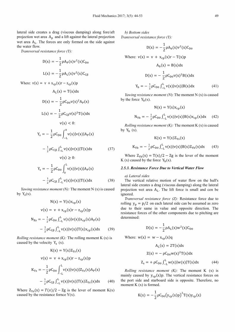
Fluid Mechanics 2017; 3(5): 44-53 49
lateral side creates a drag (viscous damping) along fore/aft
projection wet area Aa and a lift against the lateral projection
wet area AW. The forces are only formed on the side against
the water flow.
Transversal resistance force (Y):
D(x) = −12 ρAu(x)vD(x)CVs
L(x) = −12 ρAW(x)vD(x)C�]
Where: v(x) = v + x`a(x)r − z`a(x)p
AW(x) = T(x)dx
D(x) = −12 ρCVsv(x)DAu(x)
L(x) = −12 ρC�]v(x)DT(x)dx
v(x) < 0:
Y^ = −12 ρCVsy v(x)|v(x)|Au(x)s
:W
−CD ρC�] 7 v(x)|v(x)|T(x)dxW:W (37)
v(x) ≥ 0:
Y^ = −12 ρCVsy v(x)|v(x)|Au(x)W
s
−CD ρC�] 7 v(x)|v(x)|T(x)dxW:W (38)
Yawing resistance moment (N): The moment N (x) is caused
by Y^(x).
N(x) = Y(x)x`a(x) v(x) = v + x`a(x)r − z`a(x)p
N�^ = −CD ρCVs 7 v(x)|v(x)|x`a(x)Au(x)W:W
−CD ρC�] 7 v(x)|v(x)|T(x)x`a(x)dxW:W (39)
Rolling resistance moment (K): The rolling moment K (x) is
caused by the velocity Y^ (x).
K(x) = Y(x)Z�^(x) v(x) = v + x`a(x)r − z`a(x)p
K�^ = −12ρCVsy v(x)|v(x)|Z�^(x)Au(x)
W
:W
−CD ρC�] 7 v(x)|v(x)|T(x)Z�^(x)dxW:W (40)
Where Z�^(x) = {(8)/2 − Zg is the lever of moment K(x)
caused by the resistance fornce Y(x).
b) Bottom sides
Transversal resistance force (Y):
D(x) = −12 ρAe(x)vD(x)CVs
Where: v(x) = v +x`a(x)r − T(x)p
Ae(x) = B(x)dx
D(x) = −12 ρCVsv(x)DB(x)dx
Ye = −CD ρCVs 7 v(x)|v(x)|B(x)dxW:W (41)
Yawing resistance moment (N): The moment N (x) is caused
by the force Ye(x).
N(x) = Y(x)x`a(x) N�e = −CD ρCVs 7 v(x)|v(x)|B(x)x`a(x)dxW
:W (42)
Rolling resistance moment (K): The moment K (x) is caused
by Ye (x).
K(x) = Y(x)Z�^(x) K�e = −CD ρCVs 7 v(x)|v(x)|B(x)Z�e(x)dxW
:W (43)
Where Z�e(x) = T(x)/2 − Zg is the lever of the moment
K (x) caused by the force Ye(x).
2.5.3. Resistance Force Due to Vertical Water Flow
a) Lateral sides
The vertical relative motion of water flow on the hull's
lateral side creates a drag (viscous damping) along the lateral
projection wet area AW . The lift force is small and cen be
ignored.
Transversal resistance force (Z): Resistance force due to
rolling ya = p/2 on each lateral side can be assumed as zero
due to their same in value and opposite direction. The
resistance forces of the other components due to pitching are
determined:
D(x) = −12 ρAW(x)wD(x)CVs
Where: w(x) = w − x`a(x)q
AW(x) = 2T(x)dx
Z(x) = −ρCVsw(x)DT(x)dx
Z^ = +ρCVs 7 w(x)|w(x)|T(x)dxW:W (44)
Rolling resistance moment (K): The moment K (x) is
mainly caused by y`a(x)p. The vertical resistance forces on
the port side and starboard side is opposite. Therefore, no
moment K (x) is formed.
K(x) = −12 ρCVs[y`a(x)p\
DT(x)y`a(x)

50 Do Thanh Sen and Tran Canh Vinh: Establishing Mathematical Model to Predict Ship Resistance Forces
K�^ � ;CD ρCVs 7 p|p|T�x��y`a�x���dxW:W (45)
Pitching resistance moment (M): The moment M (x) on
each lateral side is caused by the force Z (x).
M�x� � ;Z�x�x`a�x� M�^ � ;ρCVs 7 w�x�|w�x�|T�x�x`a�x�dxW
:W (46)
b) Bottom side
The vertical movement of water against ship bottom mainly
create a lift on the bottom wet area Ae. The viscous resistance
component is small and can be ignored.
Vertical resistance (Z): The resistance force due to rolling
p/2 only appears on the fore or aft botom area where
impacted by the vetical water flow.
L�x� � ;12 ρAe�x�wD�x�CW]
Where: w�x� � w ; x`a�x�q; Ae�x� � CDB�x�dx
Port area: wC�x� � w ; c�d�o p ; x`a�x�q
Starboard area: wD�x� � w � c�d�o p ; x`a�x�q
Z�x� � ;12 ρCW]wC�x�D B�x�2 dx ;12 ρCW]wD�x�D B�x�2 dx
Z�x� is always negative and only appear when wC�x�> 0
or wD�x�> 0:
Z�e � ;Co ρCW] 7 �wC�x�D � wD�x�D�B�x�dxW:W (47)
Rolling resistance moment (K): The moment K (x) is
mainly due to the force B�x�p/4 forming on the fore bottom
side. The vertical resistance due to pitching on the bottom side
does not creat K (x).
K�x� � Z�x� B�x�4
Ae�x� � B�x�2 dx
K�e � ;12 ρC�]y p|p| �B�x�4 �D B�x�2
B�x�4 dx
W
:W
K�e � ; CD�� ρC�] 7 p|p|B�x��W:W (48)
Pitching resistance moment M:
The moment M (x) due to Z (x) apprear on the bottom side
at position where wC�x� > 0 or wD�x�> 0.
M�x� � Z�x�x
Z�e � Co ρC�] 7 �wC�x�D � wD�x�D�x`adxW:W (49)
2.5.4. Cross-Flow Drag
Cross-flow drag principle assumes that the sway flow of water
crossing the ship hull creates viscous drag called cross-flow drag.
Since this study for modelling ship fitted with non-conventional
propellers, the transversal speed or the |β` ;Ψ| is remarkable
and can reach 90°. Where Ψ is ship heading. Therefore, the
cross-flow drag need to be taken in account.
The Cross-flow drag is basically expressed basing on the
formula (4) [20]:
YV` � CD ρ7 U6�x�DT�x�CV��x�dxW
s (50)
Where CV��x� is cross-flow coefficient and T (x) is draft at
local section ith
. CV��x� can be predicted as:
CV� � CV�s�sinβ�x��sinβ�x� (51)
YV` � 12ρy U6�x�DCV`ssinβ�x��sinβ�x��T�x�dx
W
s
YV` � CD ρ7 CV`sT�x��v6 � xr��v6 � xr�dxW
s (52)
CV`s can be estimated as [19] by assuming the ship as
ellipsoid. Thus, KDc and NDc are calculated basing on
formula (3):
KV` � ;7 YV`z`a dxWs (53)
�U= � 7 �U=8=> 089s (54)
2.5.5. Total Damping Forces and Moments
The total damping force and moment matrix is eventually
derived :
�/ � �x � ���/ � �x � �� � �U� �/ � �x � ���/ � �x � �� � �U� �/ � �x ����/ � �x � �� � �U�
(55)
2.6. Computer Calculation and Simulation
For assessing the estimation results, some ship models are
used. This paper presents the container ship Triple-E ship
model with general particulars: L = 399m, B = 59m, T = 16m,
Displacement = 257,343MT, V = 251,067 m3.
The equations of damping coefficients are computerised with
Matlab. For this purpose, the ship is divided longitudinally into
20 sections. Lewis transformation method is used for mapping
the ship [21]. The value of added masses are calculated based
on theoretical method as the previous study in [22].
Figure 8. Overall view of the container ship Triple-E.

Fluid Mechanics 2017; 3(5): 44-53 51
Figure 9. Body plan presented using Lewis forms in Matlab.
Typical results of calculation of damping coefficients at various ship speeds (u, v) and yaw rates (rate of turn) in Matlab are
listed in the Table 2 and 3.
Table 2. Damping coefficients at various single motion parameter (straight velocity or angular velocity).
u (m/s) 5 0 0 0 0 0
v (m/s) 0 5 0 0 0 0
w (m/s) 0 0 1 0 0 0
p (rad/s) 0 0 0 10 0 0
q (rad/s) 0 0 0 0 10 0
r (rad/s) 0 0 0 0 0 10
C� -0.0024 0 0 0 0 0
C� 0 -2.0327 -2.0327 -2.0327 -2.0327 -2.9366
C� 0 0 0 0 0 0
C� 0 -0.0902 -0.0902 -0.0902 -0.0902 -0.1303
C� -0.0002 0 0 0 0 0
C 0 1.7647 1.7647 1.7647 1.7647 2.5704
Table 3. Damping coefficients with combination of various motion parameters (straight velocity and angular velocity).
u (m/s) 1 2 3 4 5 10
v (m/s) 1 2 3 4 5 10
w (m/s) 1 2 3 4 5 5
p (rad/s) 1 2 3 4 5 5
q (rad/s) 1 2 3 4 5 5
r (rad/s) 1 2 3 4 5 10
C� -0.0013 -0.0012 -0.0012 -0.0012 -0.0012 -0.0012
C� -1.2264 -1.2264 -1.2264 -1.2264 -1.2264 -1.2289
C� -2.3626 -2.3626 -2.3626 -2.3626 -2.3626 -0.5907
C� -0.0544 -0.0544 -0.0544 -0.0544 -0.0544 -0.0545
C� 1.9707 1.9707 1.9707 1.9707 1.9707 0.4926
C 1.0697 1.0697 1.0697 1.0697 1.0697 1.0719
Typical results of calculation of damping coefficients at
various ship speeds (u, v) and yaw rates (rate of turn) are also
displayed in curves by Matlab. The results indicate that the
damping coefficients are calculated reasonably.

52 Do Thanh Sen and Tran Canh Vinh: Establishing Mathematical Model to Predict Ship Resistance Forces
Figure 10. Curves of damping coefficients over u, (v=5knots, r=0 deg/m).
Figure 11. Curves of damping coefficients over v, (u=5knots, r=0 deg/m).
Figure 12. Curves of damping coefficients over r, (u=0 knot, v=0 knot).
Figure 13. Curves of damping coefficients over r, (u=5 knots, v=5 knots).
The plotting curves of damping coefficients C�, C�,C�,C�, C�, C of lift, drag, cross-flow drag and total damping
over u, v or r separately. Value u, v or r increase from minus to
plus on horizontal axis. The curves show that the coefficient
values are logically. The reasonability of the damping
coefficients is assessed basing on the results of simulating on
computer by Matlab.
3. Conclusion
The suggested equations can be used for calculating damping
coefficients of ship in 6 DOF. Mapping transformation of ship
hull combined with the suggested equations can estimate
hydrodynamic coefficients of ship’s hull to simulate the motion
of the ship with reasonable behaviour.
With mapping transformation and suggested equations to
calculate resistance coefficients, a mathematical modelling of
a ship can be made relatively fast. This method can also reduce
a quantity of complex hydrodynamic data to be transferred
into the computer. Therefore, it can reduce time for calculation
and data transaction in real-time ship simulators.
References
[1] Fossen, T. I., Handbook of Marine Craft Hydrodynamics and Motion Control. 2011, Norway: Norwegian University of Science and Technology Trondheim, John Wiley & Sons.
[2] Lewandowski, D. M., The Dynamics Of Marine Craft, Maneuvering and Seakeeping, Vol 22. Vol. 22. 2004: World Scientific.
[3] Hooft, J. P. and J. B. M. Pieffers, Manoeuvrability of frigates in waves. Marine Technology, 1998. 25 (4): p. 262-271.
[4] Sobolev, G. V. and K. Fedyayevsky, K., Control and Stability in Ship Design. 1964, Washington DC: Translation of US Dept. of Commerce.
[5] Nil Salvesen, E. O. T. and O. Faltise, Ship Motions and Sealoads. The Society of Naval Architects and Marine Engineers, No. 6., 1970.

Fluid Mechanics 2017; 3(5): 44-53 53
[6] Hine, G., D. Clarke, and P. Gedling, The Application of Manoeuvring Criteria in Hull Design Using Linear Theory. The Royal Institution of Naval Architects, 1982.
[7] Lee, T. I., On an Empirical Prediction of Hydrodynamic Coeffcients for Modern Ship Hulls. MARSIM'03, 2003.
[8] Katsuro Kijima, Y. N., On the Practical Prediction Method for Ship Manoeuvring Characteristics.
[9] Clarke, D., A two‐dimensional strip method for surface ship hull derivatives: comparison of theory with experiments on a segmented tanker model. Journal of Mechanical Engineering Science 1959-1982, 1972. 1 (23).
[10] Zelazny, K., A Method of Calculation of Ship Resistance on Calm Water Useful at Preliminary Stages of Ship Design. Scientific Journals, 2014. 38 (110): p. 125-130.
[11] Mucha, P., et al., Validation Studies on Numerical Prediction of Ship Squat and Resistance in Shallow Water, in the 4th International Conference on Ship Manoeuvring in Shallow and Confined Water (MASHCON). 2016: Hamberg, Germany.
[12] M. Ahmed, Y., et al., Determining Ship Resistance Using Computational Fluid Dynamics (CFD). Journal of Transport System Engineering, 2015. 2 (1): p. 20-25.
[13] Jaouen, F. A. P., A. H. Koop, and G. B. Vaz, Predicting Roll Added Mass and Damping of a Ship Hull Section Using CFD, in ASME 2011 30th International Conference on Ocean, O.a.A. Engineering, Editor. 2011, Marin: Rotterdam, The Netherlands.
[14] Yang, B., Z. Wang, and M. Wu, Numerical Simulation of Naval Ship's Roll Damping Based on CFD. Procedia Engineering, 2012. 37: p. 14-18.
[15] Yildiz, B., et al., URANS Prediction of Roll Damping for a Ship Hull Section at Shallow Draft. Journal of Marine Science and Technology, 2016. 21: p. 48-56.
[16] Gu, M., et al. Numerical Simulation if the Ship Roll Damping. in the 12th International Conference on the Stability of Ships and Ocean Vehincles. 2015. Glasgow, United Kingdom.
[17] Sathyaseelan, D., G. Hariharan, and G. Kannan, Parameter Identification for Nonlinear Damping Coefficient from Lasrge-smplitude Ship Roll Motion Using Wavelets. Journal of Basic and Applied Sciences, 2017. 6: p. 138-144.
[18] Abkowitz, M. A., Lectures on Ship Hydrodynamics – Steering and Maneuverability. 1964, Hydor-og Aerodynamisk Laboratorium, Report No. Hy-5.: Lyngby, Denmark.
[19] Hoerner, S. F., Fluid Dynamic Drag. Hartford House, 1965.
[20] Faltinsen, O. M., Sea Loads on Ships and Offshore Structures. Cambridge University Press., 1990.
[21] Korotkin, A. I., Added Masses of Ship Structure, in Krylov Shipbuilding Research Institute. 2009. p. 51-55, 86-88, 93-96.
[22] Thanh Sen, D. and T. Canh Vinh, Determination of Added Mass and Inertia Moment of Marine Ships Moving in 6 Degrees of Freedom. International Journal of Transportation Engineering and Technology, 2016. 2 (No. 1): p. 8-14.


![Comparative Study of Ship Resistance between Model Test ... · In their approach to establishing their formulas, Holtrop and Mennen [2,3] assumed that the non-dimensional coefficient](https://img.pdfslide.us/doc/110x75/5e0ab38e13ae20423d428ead/comparative-study-of-ship-resistance-between-model-test-in-their-approach-to.jpg)