Embed Size (px)
Citation preview

ESSAYS ON PRICE DISCRIMINATION
DONALD NGWE
Submitted in partial fulfillment of the
requirements for the degree
of Doctor of Philosophy
in the Graduate School of Arts and Sciences
COLUMBIA UNIVERSITY
2014

© 2014
DONALD NGWE
All Rights Reserved

ABSTRACT
ESSAYS ON PRICE DISCRIMINATION
DONALD NGWE
The increasing availability of detailed, individual-level data from retail settings presents
new opportunities to study fundamental issues in product design, price discrimination, and
consumer behavior. In this set of essays I use a particularly rich data set provided by a
major fashion goods manufacturer and retailer to illustrate how observed firm strategies
correspond to predictions from producer theory. I present evidence on the importance of
multidimensionality in consumer preferences, both within the theory of price discrimination
and as a factor in actual firm decisions. Finally, I explore the applicability of concepts from
signaling theory and behavioral economics in explaining consumer purchase decisions.
The first chapter describes the empirical setting used throughout the entire dissertation.
Data is provided by a luxury goods firm that dominates its category of fashion goods in the
United States. The firm operates hundreds of stores in the US, with different types of stores
differing markedly in their geographic accessibility to consumers. I present and estimate a
model of demand that admits consumer heterogeneity in two dimensions: travel sensitivity
and product age sensitivity. I show that consumer heterogeneity in these two dimensions
outweigh that in observable characteristics, such as household income. Furthermore, I esti-
mate a high correlation in the two dimensions, such that consumers who are most averse to
travel are also those for whom product newness is most valuable.
The second chapter focuses on the firm’s store location and product introduction strate-
gies. I introduce a model of product introduction wherein the firm selects only the param-
eters of the distribution of product characteristics, rather than the characteristics of each
new product. This dramatically simplifies the firm’s optimization program. I use this model

to simulate counterfactual product assortments given alternative store location decisions. I
show that the optimality of observed store locations depends substantially on the correlation
in consumer values for travel distance and product quality. I also show that increased dif-
ferentiation in geographic accessibility enables the firm to profitably increase differentiation
in product quality.
The third chapter studies how consumers respond to different price signals conditional on
store visitation. Many firms employ price comparisons as a selling strategy, in which actual
prices are framed as discounted from a high list price, occasionally even when no units are
sold at list prices. I show that high list prices enhance demand both on product and store
levels. I present evidence that suggests that consumers infer quality from list prices. I also
demonstrate that these demand-enhancing effects are dependent on characteristics of the
retail context, such as the general level and dispersion of discounting.
These essays study in isolation components of consolidated selling strategies that have
been widely adopted by US manufacturers and retailers across a wide variety of categories.
My hope is to achieve a deeper understanding of the aspects of consumer behavior and firm
incentives that have led to the prevalence of these selling strategies. This understanding is
central in forming prescriptions for managers as well as measuring welfare implications, both
of which I leave for future work.

Table of Contents
List of Tables iii
List of Figures v
Acknowledgments vi
1 Why Outlet Stores Exist:
Market Segmentation in Unobservable Consumer Attributes 1
1.1 Introduction . . . . . . . . . . . . . . . . . . . . . . . . . . . . . . . . . . . . 2
1.2 Related literature . . . . . . . . . . . . . . . . . . . . . . . . . . . . . . . . . 3
1.3 Data and industry background . . . . . . . . . . . . . . . . . . . . . . . . . . 6
1.4 Preliminary evidence . . . . . . . . . . . . . . . . . . . . . . . . . . . . . . . 9
1.4.1 Inventory management . . . . . . . . . . . . . . . . . . . . . . . . . . 9
1.4.2 Geographic segmentation . . . . . . . . . . . . . . . . . . . . . . . . . 11
1.4.3 Consumer self-selection . . . . . . . . . . . . . . . . . . . . . . . . . . 16
1.5 Demand . . . . . . . . . . . . . . . . . . . . . . . . . . . . . . . . . . . . . . 16
1.6 Conclusion . . . . . . . . . . . . . . . . . . . . . . . . . . . . . . . . . . . . . 22
2 Why Outlet Stores Exist:
Store Location and Product Assortment 23
i

2.1 Introduction . . . . . . . . . . . . . . . . . . . . . . . . . . . . . . . . . . . . 24
2.2 Supply . . . . . . . . . . . . . . . . . . . . . . . . . . . . . . . . . . . . . . . 25
2.3 Policy Simulations . . . . . . . . . . . . . . . . . . . . . . . . . . . . . . . . 33
2.3.1 No outlet stores . . . . . . . . . . . . . . . . . . . . . . . . . . . . . . 34
2.3.2 Random assortment . . . . . . . . . . . . . . . . . . . . . . . . . . . 37
2.3.3 Centrally-located outlet stores . . . . . . . . . . . . . . . . . . . . . . 39
2.4 Conclusion . . . . . . . . . . . . . . . . . . . . . . . . . . . . . . . . . . . . . 42
3 Discount Pricing in Retail 45
3.1 Introduction . . . . . . . . . . . . . . . . . . . . . . . . . . . . . . . . . . . . 46
3.2 Related literature . . . . . . . . . . . . . . . . . . . . . . . . . . . . . . . . . 48
3.3 Data and industry background . . . . . . . . . . . . . . . . . . . . . . . . . . 53
3.4 Demand model . . . . . . . . . . . . . . . . . . . . . . . . . . . . . . . . . . 57
3.5 Conclusion . . . . . . . . . . . . . . . . . . . . . . . . . . . . . . . . . . . . . 70
Bibliography 71
Appendices 77
Appendix A Appendix for Chapter 1 78
A.1 Estimation of taste covariance matrix . . . . . . . . . . . . . . . . . . . . . . 78
A.2 Alternative covariance specifications . . . . . . . . . . . . . . . . . . . . . . . 78
Appendix B Appendix for Chapter 2 82
B.1 Finding optimal prices . . . . . . . . . . . . . . . . . . . . . . . . . . . . . . 82
Appendix C Appendix for Chapter 3 83
ii

List of Tables
1.1 Average Store Characteristics . . . . . . . . . . . . . . . . . . . . . . . . . . 8
1.2 Inventory Flows . . . . . . . . . . . . . . . . . . . . . . . . . . . . . . . . . . 10
1.3 Average Consumer Characteristics by Store Format . . . . . . . . . . . . . . 12
1.4 Consumer behavior . . . . . . . . . . . . . . . . . . . . . . . . . . . . . . . . 12
1.5 Average Market Characteristics . . . . . . . . . . . . . . . . . . . . . . . . . 13
1.6 Pricing equation . . . . . . . . . . . . . . . . . . . . . . . . . . . . . . . . . . 19
1.7 Demand estimates . . . . . . . . . . . . . . . . . . . . . . . . . . . . . . . . 20
1.8 Market segmentation by consumer tastes . . . . . . . . . . . . . . . . . . . . 21
2.1 Implied product development costs . . . . . . . . . . . . . . . . . . . . . . . 33
2.2 Test market store characteristics . . . . . . . . . . . . . . . . . . . . . . . . . 35
2.3 No outlet stores (supply response) . . . . . . . . . . . . . . . . . . . . . . . . 36
2.4 No outlet stores (demand response) . . . . . . . . . . . . . . . . . . . . . . . 37
2.5 Randomized product distribution–supply . . . . . . . . . . . . . . . . . . . . 38
2.6 Randomized product distribution (actual tastes) . . . . . . . . . . . . . . . . 39
2.7 Randomized product distribution (uncorrelated tastes) . . . . . . . . . . . . 40
2.8 Outlet moved to center (supply response) . . . . . . . . . . . . . . . . . . . . 41
3.1 Average prices in outlet format . . . . . . . . . . . . . . . . . . . . . . . . . 55
iii

3.2 Sample descriptive statistics . . . . . . . . . . . . . . . . . . . . . . . . . . . 59
3.3 Demand estimates . . . . . . . . . . . . . . . . . . . . . . . . . . . . . . . . 60
3.4 New vs old consumers . . . . . . . . . . . . . . . . . . . . . . . . . . . . . . 63
3.5 Pure factory vs full price shoppers . . . . . . . . . . . . . . . . . . . . . . . . 63
3.6 Interaction . . . . . . . . . . . . . . . . . . . . . . . . . . . . . . . . . . . . . 64
3.7 Consumer sensitivity to list prices . . . . . . . . . . . . . . . . . . . . . . . . 65
3.8 Description of variable labels in Table 3.9 . . . . . . . . . . . . . . . . . . . . 66
3.9 Reference points . . . . . . . . . . . . . . . . . . . . . . . . . . . . . . . . . . 67
3.10 Past-period price effects . . . . . . . . . . . . . . . . . . . . . . . . . . . . . 69
A.1 Nonzero covariance in price and distance coefficients . . . . . . . . . . . . . . 79
A.2 Nonzero covariance in price and product age coefficients . . . . . . . . . . . . 80
C.1 Frequency of list prices . . . . . . . . . . . . . . . . . . . . . . . . . . . . . . 83
C.2 Traffic . . . . . . . . . . . . . . . . . . . . . . . . . . . . . . . . . . . . . . . 84
C.3 First stage IV regressions . . . . . . . . . . . . . . . . . . . . . . . . . . . . . 85
C.4 Shifting with store average discount percent . . . . . . . . . . . . . . . . . . 87
iv

List of Figures
1.1 Product flows . . . . . . . . . . . . . . . . . . . . . . . . . . . . . . . . . . . 10
1.2 Consumers in Indianapolis, IN . . . . . . . . . . . . . . . . . . . . . . . . . . 14
1.3 Outlet store revenues in Indianapolis, IN . . . . . . . . . . . . . . . . . . . . 15
2.1 Empirical versus simulated age densities in primary format . . . . . . . . . . 30
2.2 Empirical versus simulated age densities in outlet format . . . . . . . . . . . 31
2.3 Better products are longer-lived in primary stores . . . . . . . . . . . . . . . 32
2.4 Central outlet policy vs taste correlation . . . . . . . . . . . . . . . . . . . . 42
3.1 Consumers by number of within-sample purchase instances . . . . . . . . . . 54
3.2 Discounting pattern in outlet channel . . . . . . . . . . . . . . . . . . . . . . 55
3.3 Discounting pattern of a typical good . . . . . . . . . . . . . . . . . . . . . . 56
C.1 Average discount percent in outlet stores . . . . . . . . . . . . . . . . . . . . 84
C.2 Average discount percent in outlet stores . . . . . . . . . . . . . . . . . . . . 85
C.3 Scatterplot of suggested prices and estimated quality . . . . . . . . . . . . . 86
C.4 Prices over time . . . . . . . . . . . . . . . . . . . . . . . . . . . . . . . . . . 88
v

Acknowledgments
I am grateful to Chris Conlon, Brett Gordon, Kate Ho, Mike Riordan, and Scott Shriver for
their invaluable advice, support, and encouragement.
I also thank the many faculty members and students at Columbia who have contributed
to my work, including Jisun Baek, Alejo Czerwonko, Jonathan Dingel, Ronald Findlay, Jessie
Handbury, Corinne Low, Wataru Miyamoto, David Munroe, Serena Ng, Thuy Lan Nguyen,
Giovanni Paci, Bernard Salanie, Patrick Sun, and Zhanna Zhanabekova.
vi

Chapter 1
Why Outlet Stores Exist:
Market Segmentation in Unobservable
Consumer Attributes

2
1.1 Introduction
Outlet stores are a fixture of the American retail landscape. These are brick-and-mortar
stores that offer deep discounts in locations far away from most consumers. Firms operate
outlet stores in addition to primary stores, which are located in central shopping districts.
Outlet stores operated by different firms are often agglomerated in sprawling outlet malls
off interstate highways. In 2012 there were 185 outlet malls in the US, which generated an
estimated $25.4 billion in revenues (Humphers 2012).
There are several perspectives on why outlet stores have become a widely adopted selling
strategy. The first is inventory management : outlet stores provide firms with a cost-efficient
way to dispose of excess inventory. The second is geographic segmentation: outlet stores
cater to lower-value consumers that reside around outlet malls. The third is consumer self-
selection: lower-value consumers travel greater distances to avail of discounted products.
In this and the following chapter, I evaluate the relevance of each of these proposed
explanations to the case of a major fashion goods firm with a heavy outlet store presence.
Using new and highly granular data, I am able to observe both inventory flows between store
formats, and locations and sales records of individual consumers—rich sources of model-free
evidence. I then make use of structural models of demand and supply to predict consumer
behavior and firm product decisions under counterfactual store configurations.
It is evident from observing product flows alone that inventory management is not an
essential function of the firm’s outlet stores. The firm sells a significant fraction of units of
each style through the outlet channel. It is also immediately clear that outlet stores do not
primarily serve the communities in their vicinity—most of each outlet store’s revenues are
attributed to consumers for whom a primary store is closer to home. This suggests that the
firm’s main motivation for operating outlet stores might be to price discriminate among its

3
consumers by forcing the most price-sensitive among them to travel to obtain discounts.
Surprisingly, consumers who shop at outlet stores do not differ significantly from con-
sumers who shop at primary stores in terms of observable characteristics such as income.
They make purchases at roughly the same frequency, and have had about the same time
elapse since their first purchase of the brand. Taking these factors into account, I propose
a demand model that characterizes how consumers make their purchase decisions. I use the
demand model to estimate the extent to which consumers vary in their unobservable charac-
teristics, and to show that outlet store consumers differ from primary store consumers in two
ways: their sensitivity to travel distance and their taste for product newness. In addition, I
find a strong positive correlation between these two values.
This chapter proceeds as follows. I review the related literature in Section 1.2. In Section
1.3, I describe the data. In Section 1.4, I provide preliminary evidence of how outlet stores
work. In section 1.5, I outline the demand model I use to estimate preferences, discuss the
estimation procedure, and present the estimates. Section 1.6 concludes.
1.2 Related literature
This work contributes to several literatures in marketing and economics. It is the first
empirical study to study the incentives behind outlet store retail. It builds on existing work
on product line decisions. It proposes a technique to model endogenous product choice
for cases in which a large number of products comprise each product line. The underlying
structure of the firm’s problem that I model belongs to the class of multidimensional screening
models, for which few general results are available and no empirical work has been performed.
Finally, this and the next chapter demonstrate that outlet stores allow the firm to improve
quality in its primary stores, which may countervail brand dilution.

4
Several theories exist about how why firms build and sell goods through outlet stores.
Deneckere and McAfee (1996) derive conditions under which a firm would damage or “crimp”
a portion of its goods to increase profits by expanding its market share, and put forth outlet
stores as an example of such a damaged goods strategy. This work picks up this example and
provides the first empirical demonstration of a successful damaged goods policy. Coughlan
and Soberman (2005) show that dual distribution (i.e. having both primary and outlet stores)
is more profitable than single channel distribution when the range of service sensitivity is
low relative to the range of price sensitivity. While these sensitivities were independent in
their model, I look chiefly at how the correlation between consumer sensitivities matters.
In recent empirical work, Qian et al. (2013) show that the opening of an outlet store had
substantial positive spillovers for a retailer’s primary channel, and ascribe this spillover to
the advertising effects of a new store opening. This essay goes further by studying how the
firm’s optimal product line choices are influenced by its store locations—thereby offering an
alternative mechanism by which outlet stores can have positive spillovers.
More generally, this work offers a new point of view on how product lines should be
designed to effectively segment consumers. Previous work on product line design has explored
the benefits of broadening product lines (Kekre and Srinivasan 1990; Bayus and Putsis 1999),
methods for selecting optimal product lines (Moorthy 1984; Green and Krieger 1985; McBride
and Zufryden 1988; Dobson and Kalish 1988; Netessine and Taylor 2007), cannibalization
between product lines (Desai 2001), pricing (Reibstein and Gatignon 1984; Draganska and
Jain 2006), and the effects on brand equity of product line extensions (Randall, Ulrich,
and Reibstein 1998). These essays contribute to this body of work by demonstrating the
importance of accounting for the full extent of consumer heterogeneity in making product
line decisions. It also shows how concerns like cannibalization can be ameliorated by a careful
design of product line attributes.
5
I develop an explicit model of product line choice that corresponds to the institutional
details of the fashion goods industry. The large number of products in each product line poses
a particular challenge. While existing work has modeled endogenous product choice for a
single multidimensional good (Fan 2010) or for several single-dimensional goods (Draganska,
Mazzeo, and Seim 2010; Crawford, Shcherbakov and Shum 2011), none has addressed the
product choice problem of a firm with several multidimensional products. I introduce a
simple and tractable method of describing this choice. Modeling the firm as choosing the
parameters of a distribution of product characteristics, rather than the characteristics that
make up each individual product, dramatically reduces the number of choice variables for
the firm. It may also be a more realistic representation of decision-making in many sectors.
The importance of allowing product design to be endogenously determined in equilibrium
has been emphasized in many recent papers. Kuksov (2004) shows that firms may respond
to lower buyer search costs by increasing product differentiation and thus diminishing price
competition. There are many other instances in which allowing for endogenous product
differentiation changes the sign of welfare effects.
This and the next chapter’s central premise is that the choice of whether to open outlet
stores and what to stock them with is a type of multidimensional screening problem. Em-
pirical models of multidimensional product choice are particularly useful because they can
be used to complement lessons from theoretical work in multidimensional screening. The
obstacles to obtaining general results in multidimensional screening are well-documented
by Rochet and Stole (2003). Full solutions to this problem are available for the discrete
two-by-two-type case (Armstrong and Rochet 1999) and other cases for which the form of
consumer heterogeneity is severely restricted (e.g. Armstrong 1996). It is difficult to see
how these models’ predictions would manifest in actual product decisions, such as those in
my empirical setting. By using demand and supply models that are not anchored to any

6
particular screening model, I am able to provide evidence for the applicability of existing
results to real world settings and the significance of multidimensional screening for firms in
general.
1.3 Data and industry background
The first outlet stores appeared in the Eastern United States in the 1930s. These stores
were attached to factories and sold overruns, irregulars, and slightly damaged goods. Outlet
stores initially catered to only the firm’s employees, but the stores’ market audience quickly
expanded to include regular consumers. Until the 1970s, firms continued to use outlet stores
primarily to dispose of excess inventory, even as they established them independently of
manufacturing centers.
The modern outlet store has evolved into a considerably different format from its earlier
incarnations. In many ways, outlet store goods now constitute distinct product lines, rather
than mere excess inventory. Many firms design products exclusively for sale in outlet stores
(though they may prefer to limit awareness of the practice among consumers). Revenues
from outlet stores often rival, and sometimes exceed, revenues from a firm’s primary retail
formats.
One feature of the outlet store that remains unchanged is its distance from central shop-
ping districts. In fact, an entire industry of outlet mall operators owes its existence to the
prevalence of this selling strategy among clothing and fashion goods retailers. The practice
of selling goods in hard-to-access locations would seem curious were it not so common. De-
neckere and McAfee (1996) provide a relevant argument in this regard by showing that a firm
may profit from “damaging” a portion of its goods. They also point out that the practice
is widespread: certain slower microprocessors, student editions of software, and outlet store
7
offerings can all be considered damaged goods.
Yet many firms choose not to sell through outlet stores; adoption is variable even within
narrowly-defined categories. For instance, premium apparel manufacturers Brooks Brothers,
Hugo Boss, and Ralph Lauren have several outlet store locations, but Chanel, Burberry and
Zegna have few or none. Coughlan and Soberman (2005) provide an explanation for this fact
that rests on the form of consumer heterogeneity. They show that firms find single-channel
distribution superior when the range of service sensitivity among consumers is high relative
to the range of price sensitivity.
The data used for this study consists of transaction-level records from July 2006 to
March 2011. About 60% of the firm’s revenues are sales of its main category; the remainder
is from sales of other categories. The sample includes all purchases of products made by US
consumers in firm-operated channels. Excluded from this sample are online and department
store sales, which according to the firm’s managers accounted for less than 10% of total
revenue.
The firm is able to track repeat purchase behavior by consumers. Available information
on consumers includes their billing zip codes, date of first purchase at a store, and their total
lifetime expenditures on the firm’s products. Each record contains detailed information
on the consumer, the product, and the store. Product attributes include color, silhouette,
materials, collection, release date, and a code that uniquely identifies each style. Store
attributes include their location, weeklong foot traffic, and format type.
For the analysis in this essay, I focus on main category purchases in physical stores.
While this excludes a considerable number of other-category purchases, those observations
are used to proxy for the number of consumers who visit a store but do not make a main
category purchase.
The firm’s overall distribution strategy is fairly typical among brands with outlet store
8
locations. The firm introduces most of its new products in its primary stores, which are
located in central shopping districts. After a few months, these products are pulled out of
the primary stores and transferred to the outlet stores. The firm also produces styles that
are sold exclusively in outlet stores.
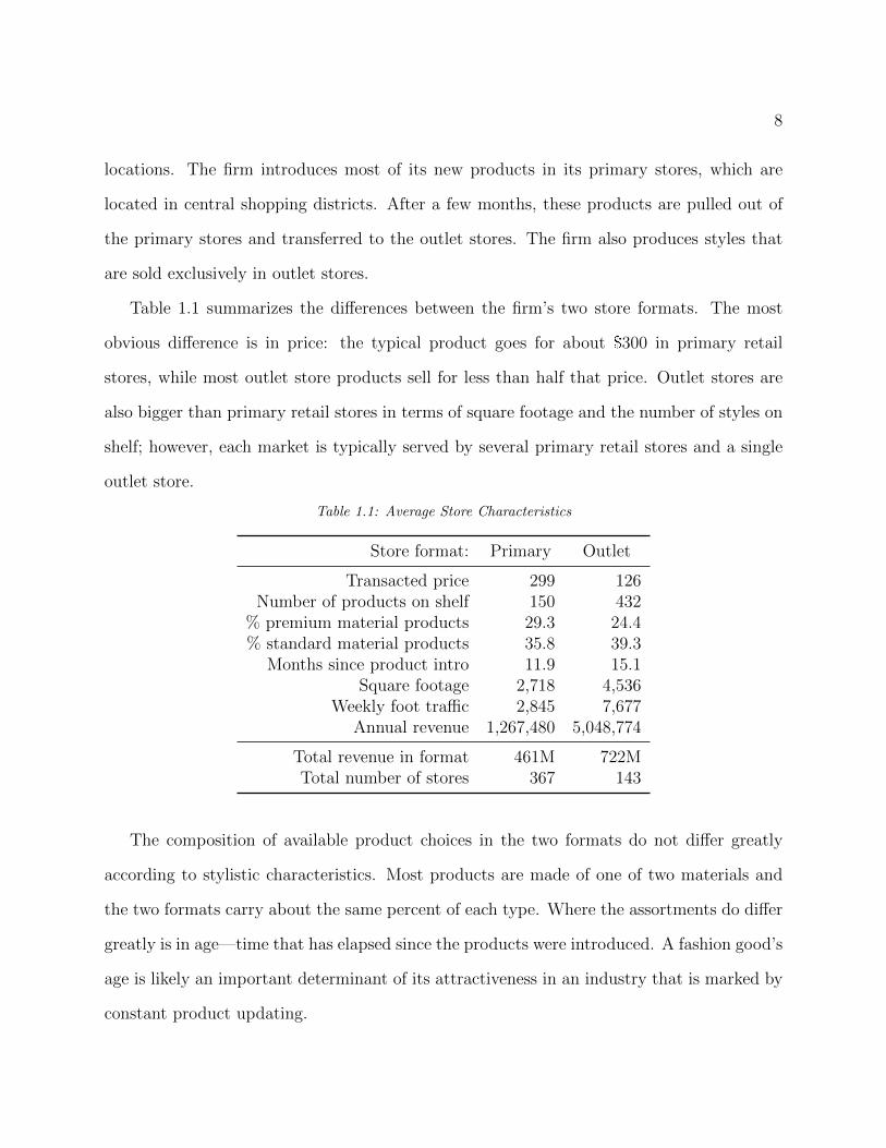
Table 1.1 summarizes the differences between the firm’s two store formats. The most
obvious difference is in price: the typical product goes for about $300 in primary retail
stores, while most outlet store products sell for less than half that price. Outlet stores are
also bigger than primary retail stores in terms of square footage and the number of styles on
shelf; however, each market is typically served by several primary retail stores and a single
outlet store.
Table 1.1: Average Store Characteristics
Store format: Primary Outlet
Transacted price 299 126Number of products on shelf 150 432
% premium material products 29.3 24.4% standard material products 35.8 39.3
Months since product intro 11.9 15.1Square footage 2,718 4,536
Weekly foot traffic 2,845 7,677Annual revenue 1,267,480 5,048,774
Total revenue in format 461M 722MTotal number of stores 367 143
The composition of available product choices in the two formats do not differ greatly
according to stylistic characteristics. Most products are made of one of two materials and
the two formats carry about the same percent of each type. Where the assortments do differ
greatly is in age—time that has elapsed since the products were introduced. A fashion good’s
age is likely an important determinant of its attractiveness in an industry that is marked by
constant product updating.

9
1.4 Preliminary evidence
In this section I use a descriptive analysis of the data to offer preliminary evidence of the
value to the firm of having outlet stores. In each subsection, I provide model-free evidence
that speaks to each of three main possible purposes: inventory management, geographic
segmentation, and consumer self-selection.
1.4.1 Inventory management
I first consider the relevance of outlet stores in managing the firm’s inventory: particularly
the disposal of excess supply. This purpose serves as the historical basis for outlet stores’
emergence, and continues to be relevant for many firms. As I show in the following discussion,
however, inventory management does not appear to be a primary purpose of the firm’s outlet
stores.
At the most basic level, the firm manufactures two types of products, which I term
original and factory. Original products are introduced in the primary stores, and after a
few months, taken out of primary stores and sold in outlet stores. Factory products are sold
only in outlet stores. Figure 1.1 summarizes these flows. At any given point, an outlet store
offers about as many original products as factory products. While original products are
typically thought of as more desirable than factory products, anecdotal evidence suggests
that consumers are seldom able to distinguish one from the other, or even aware of the
distinction. Table 1.2 contains information on the flows of these product types.
Inspecting product flows alone suggests that the firm does not use outlet stores for the
traditional purpose of disposing of excess inventory. First, it is not the firm’s policy to sell
defective merchandise in either of its channels. Second, the firm manufactures a product line
that is meant for exclusive sale in its outlet stores. And third, close to half of the units of

10
Figure 1.1: Product flows
Table 1.2: Inventory Flows
Product type: Original Factory
Average styles introduced per year 336 132Average months sold in primary format 10.32 N/A
Average months sold in outlet format 6.97 11.03Average total units per style sold in primary format 3,103 N/A
Average total units per style sold in outlet format 2,707 12,725Average composition of styles in outlet format (%) 42.71 57.29

11
each style that is introduced in primary stores is sold in outlet stores. This implies that the
life of “original” products in outlet stores represents a deliberate aging strategy rather than
a dump of excess inventory.
1.4.2 Geographic segmentation
Given how the firm uses location to distinguish each product line, a natural hypothesis is
that outlet stores are designed to segment consumers according to geography. In fact, outlet
stores are located in areas that have lower population density and lower income than the
areas around primary stores.
Table 1.3 catalogues average consumer characteristics in each format that are observable
in the data. The averages are taken over all purchases in each format. Median household
incomes by zip code from the 2010 American Community Survey are used to proxy for a
consumer’s income. The consumer’s travel distance is the distance between centroids of the
consumer’s billing zip code and the store’s zip code.
Noteworthy in Table 1.3 is the absence of an appreciable difference in observable charac-
teristics between consumers who buy from the two formats. They resemble each other not
only in income, but also in their level of experience with the firm’s products. As will be
clear from the succeeding discussion, the difference in travel distance reflects the fact that
consumers in both formats live in the same areas, but must travel farther to access outlet
stores.
An alternative way of thinking about classes of consumers is presented in Table 1.4. In
this table, I consider consumers who have made at least two purchases in the sample and
group them according to the store formats at which they made the transactions. Consumers
either shopped at exclusively one format, or at both formats. Share refers to what percent of
all consumers belongs to each class. Outlet closer is the percent of each class of consumers

12
Table 1.3: Average Consumer Characteristics by StoreFormat
Store format: Primary Outlet
Income 71,231 65,226(27,780) (23,670)
Years since first purchase 2.51 2.25(3.40) (3.08)
Travel distance 9.53 20.44(8.49) (15.65)
Standard deviations are in parentheses.
for whom the closest store is an outlet. The main takeaway from Table 1.4 is that even
within the class of consumers who shop exclusively at outlet stores, 70.5 percent live closer
to primary stores.
Table 1.4: Consumer behavior
Only primary retail Only outlet store Multi-home
Share (%) 13.2 56.8 30.0Outlet closer (%) 7.0 29.5 15.3
Average income ($) 73,489 64,554 69,294
I take a core-based statistical area (CBSA) to be a reasonable geographic market defini-
tion.1 I choose months as a temporal market definition. While perhaps a shorter time period
than actual consumers take to return to the market, rapidly changing choice sets necessitate
a tightly defined market period. Table 1.5 has descriptive statistics for the average market
according to my definition.
Figure 1.2 identifies where the firm’s consumers live in Indianapolis, Indiana and shows
the market population density by zip code. Indianapolis is a typical market for the firm,
which it serves with two primary store locations and one outlet store. For the purposes
1CBSAs consist of metropolitan statistical areas and micropolitan areas–collectively areas based on urbancenters of at least 10,000 people and economically relevant adjoining areas.

13
Table 1.5: Average Market Characteristics
Mean St Dev
Number of primary stores 1.96 3.52Number of outlet stores 0.66 0.66
Revenue 186,666.00 371,510.50Market size (#consumers) 92,870.51 186,769.80
A market is a CBSA-month.
of this figure, a ‘consumer’ is an individual who purchased at least one item from the firm
within the five-year sample.
Figure 1.2 highlights the fact that the outlet store is located in an area where very few
consumers reside. This agrees with what is found in the national sample, where there is a
relatively small group of consumers for whom the closest store is an outlet store.
Figure 1.3 shows from where revenues at the outlet store are sourced. The shading of the
regions closely resembles the market population density shown in Figure 1.2. Most of the
outlet store’s revenues are attributed to consumers who live in the central shopping district
where the primary stores are located. As before, this is a pattern that is also seen in the
national sample.
By inspecting the data alone, it can reasonably be inferred that geographic market seg-
mentation is not a driver of the outlet store strategy. The two store formats serve nearly
identical locations, and often attract the same consumers. This leaves one last hypothesis
to consider: that the firm’s selling strategy is designed to implement price discrimination
through consumer self-selection.2
2Here ‘geographic segmentation’ is taken to be synonymous with third-degree price discrimination, and‘self-selection’ with second-degree price discrimination.

14
Figure 1.2: Consumers in Indianapolis, IN

15
Figure 1.3: Outlet store revenues in Indianapolis, IN

16
1.4.3 Consumer self-selection
This chapter focuses on illustrating how outlet stores induce a segment of consumers to travel
for discounts. While, as Tables 1.3 and 1.4 show, consumers do not markedly differ in their
observable attributes by format choice, this does not preclude them from differing in their
preferences. In the following section, I lay out a demand model that permits heterogeneity
in unobserved consumer tastes. Among other uses, estimation of the model’s parameters will
allow me to more fully characterize the differences in primary store and outlet store patrons.
This step illustrates how the firm’s selling strategy achieves a sorting of consumers according
to their preferences.
1.5 Demand
In this section, I present a model of demand for the firm’s main category, which takes on a
nested mixed logit form. I proceed to discuss how I estimate the parameters of the model
using transactions data from the firm. Finally, I present the results of demand estimation and
discuss what they imply about the function of outlet stores as a tool for price discrimination.
Demand model. Since the typical consumer chooses between multiple locations, it is
natural to think of her purchase decision as consisting of a store choice followed by a product
choice. Conditional on her store choice, the indirect utility that a consumer i derives from
purchasing product j in month t is
uijt = ξj − (α + ζi)pjt − (β + ηi)agejt + εijt. (1.1)
That is, her utility is determined by: the intrinsic quality of the product, ξj; the product’s
price pjt at time t; time that has elapsed since the product was introduced, denoted agejt; and

17
an idiosyncratic demand shock εijt. I assume that consumers vary in their price sensitivity
according to deviations ζi from the mean level α, and in their taste for new products according
to deviations ηi from the mean level β. Utility from the outside good is normalized to
ui0t = εi0t. I also assume that εijt is i.i.d. type-I extreme value.
At the store, the consumer chooses the product that gives her the highest utility.3 Given
the distributional assumption on εijt, this implies that the expected utility consumer i derives
from a store k’s product assortment in month t, Jkt, is the inclusive value
IVikt = log
(∑h∈Jkt
exp(ξh − (α + ζi)pht − (β + ηi)ageht)
). (1.2)
Consumers choose which store to visit based on store characteristics in addition to their
expected utility from the available products. Consumer i’s utility from visiting store k in
month t is
uikt = ξk + λIVikt − (γ + νi)distanceik + εikt. (1.3)
A desirable feature of the data is that each consumer’s billing zip code is observed,
allowing for a focus on the role of travel distance in consumer choices. In addition, I allow
for individual deviations νi from the mean level of sensitivity to travel γ. The parameter
λ governs substitution patterns between products and stores by indicating the correlation
in unobserved product characteristics within each store. The fixed effect ξk captures the
attractiveness of features of store k that are unrelated to the products within it or its
distance from consumers. I normalize utility from no store visit to ui0t = εi0t and again
assume that εikt is i.i.d type-I extreme value.
These distributional assumptions imply that the probability that consumer i purchases
3Unit demand is appropriate given that 99.4% of all transactions in the data are single-unit purchases.

18
product j in store k in month t is
Pit(jk) = Pit(j|k)Pit(k) (1.4)
=exp(ξj − (α + ζi)pjt − (β + ηi)agejt)
1 +∑
h∈Jkt exp(ξh − (α + ζi)pht − (β + ηi)ageht)(1.5)
× exp(ξk + λIVikt − (γ + νi)distanceik)
1 +∑
l∈Kiexp(ξl + λIVilt − (γ + νi)distanceil)
(1.6)
where Ki is the set of stores in consumer i’s market.
I further assume that ζi ∼ N(0, σ) and [ ηi νi ]′ ∼ N(0,Σ). This allows for a nonzero
correlation between sensitivity to travel and taste for new products. In this version of the
model, correlations with the price coefficient are restricted to zero. These restrictions are
partially relaxed in the appendix, which also contains a discussion of possible implications
of these assumptions (see Section A.2).
Note that, based on the specified model and the granularity of the data, consumers are
identical up to their billing zip codes. Consequently, the predicted market share of product
j in store k at the zip code z where consumer i resides is
szt(jk) =
∫i
Pit(jk)df(ζi, ηi, νi;σ,Σ), (1.7)
where f is a multivariate normal pdf.
Let nzjkt be the number of consumers in zip code z that purchase product j at store k
in month t. The log-likelihood function given a set of parameter values and fixed effects
Θ = (α, β, γ, λ, σ,Σ, {ξj}, {ξk}) is
l(Θ) =∑t
∑k∈Kz
∑j∈Jkt
∑z
nzjkt log szt(jk), (1.8)

19
where Kz is the set of stores geographically accessible from zip code z.
Market sizes and outside options. For estimation purposes, the market size for each
zip code is the total number of unique consumers who made a purchase within the entire
sample. That assumption is that consumers who do not make a purchase over a five-year
period are not part of the market. If a consumer purchases an other-category product from
store k, then she is counted as visiting store k and choosing the outside option. If a consumer
is not observed during a period, then she is counted as not having visited a store.
Identification. The firm’s pricing practices allows for the consistent estimation of α
and σ without the use of instrumental variables techniques. To begin with, the firm im-
plements a national pricing regime, thereby eliminating any systematic pricing differences
between markets. Within-product variation in prices is generated by two sources. The first
is randomly implemented store-wide promotions. These typically take the form of discounts
that apply to all of the products in-store. The second is a systematic marking down of prod-
ucts over time. Table 1.6 shows through a projection of prices on product fixed effects, an
outlet dummy, and age that most of the variation in prices is accounted for by the included
variables, while the leftover variation falls within the scope of the randomized promotions.
Table 1.6: Pricing equation
Variable Coefficient St Dev
constant 5.33 0.15outlet -0.42 0.0029
log(age) -0.43 0.0022
depvar log(price)product FE yes
R2 0.8965
The inclusion of product and store fixed effects in the estimation absorbs all unobserved
quality differences between products and stores outside of age and distance. This also ad-

20
dresses potential endogeneity concerns with respect to the assignment of products to partic-
ular stores.
Table 1.7 outlines the result of the estimation procedure. All estimated coefficients have
the expected sign: higher prices, older ages, and farther distances adversely affect utility.
The Choleski decomposition of covariance matrix Σ is precisely estimated and implies a
large variance in travel sensitivity and taste for new products. The estimates indicate a high
correlation between travel sensitivity and taste for new products: consumers who highly
dislike traveling also dislike buying old merchandise.
Table 1.7: Demand estimates
coef se
Product levelprice -2.327 0.503σprice 0.344 0.109
age -2.621 0.681Store level
IV 0.442 0.183distance -0.912 0.079
chol(Σ)(1,1) 0.908 0.297(2,1) 0.435 0.178(2,2) 0.209 0.172
Implied covariancesσage 0.908σdist 0.483
ρage,dist 0.629
N 7,566,195l 1,832.09
product fixed effects yesstore fixed effects yes
An interpretation of the estimated coefficients for price, age, and distance is that the
average consumer would have to be compensated roughly $100 in order to maintain her level

21
of utility given a one-year increase in the age of a product or a 20-mile increase in travel
distance. The λ estimate implies a moderate correlation in demand shocks within each store.
Market segmentation. Estimating the underlying parameters of consumer preferences
allows for a description of consumers based on unobservable characteristics. Here I use the
estimates to expound on the differences between consumers who buy goods from primary
stores and those who buy goods from the outlet stores. I do this by using my demand model
to predict purchase behavior given the available products for different types of consumers.
Recall that consumers and their choices differ in multiple ways: (1) within each market,
they vary by home zip code and thus perceive relative travel distances differently, (2) store
availability and assortment differ between markets, and (3) consumers in all locations differ
in their travel sensitivity and taste for new products.
Table 1.8 adds to the information in Table 1.3 through demand estimation. Whereas the
data shows that consumers do not significantly differ by income and other purchase behavior
depending on which format they choose, estimation reveals that they differ greatly in travel
sensitivity and taste for new products.
Table 1.8: Market segmentation by consumer tastes
Consumer values ($) for: Primary Stores Outlet Stores
20-mile travel distance increase 71.83 36.21(12.47) (11.08)
1-year product age increase 51.97 33.45(14.22) (12.76)
This table lists consumer values in dollars for changes in store and productattributes. Standard errors are in parentheses.

22
1.6 Conclusion
The analysis in this section provides supportive evidence that through the firm’s outlet
store strategy, it segments consumers according to their underlying preferences for travel
and product newness. Discounts in outlet stores seem deep enough to cater to lower-value
consumers, but not enough to cater to consumers who place a high premium on convenience
and new arrivals.
The demand estimates suggest an important role for estimation of unobservable con-
sumer characteristics in evaluating market segmentation efforts. In the current setting, mere
inspection of consumer income underestimates the extent of consumer heterogeneity between
retail channels. Demand estimation can also conceivably provide retailers with guidance as
to which of several consumer attributes drives heterogeneity in their particular markets, and
consequently, which product characteristics can most effectively maximize product differen-
tiation.
A complete argument for these conclusions requires studying counterfactual store con-
figurations and the associated consumer responses. The natural counterfactual scenario is
one in which the firm chooses not to open locations in outlet malls. It would be insufficient,
however, to simply remove these locations from the data and simulate purchase behavior.
The firm would presumably charge different prices in its primary stores in the absence of
outlet stores. Since outlet stores form an integral part of the firm’s distribution strategy,
removing them would also motivate changes in the how the firm stocks its primary stores.
The following chapter provides a framework for thinking about how the firm chooses
prices and product assortments given its dual distribution strategy. The purpose of these
models is to form a basis, together with the demand model, for predicting firm performance
given a counterfactual distribution strategy.

Chapter 2
Why Outlet Stores Exist:
Store Location and Product
Assortment

24
2.1 Introduction
As in many other retail settings, there is a clear relationship between store and product
attributes in the current setting’s dual distribution framework. Primary stores stock new
arrivals, while older products are sold in outlet stores. I hypothesize that the firm exploits
the positive correlation between consumer travel sensitivity and taste for new products by
selling older products in its outlet stores. I test this notion by setting the correlation to zero
and simulating the corresponding purchase behavior. I find that the resulting advantage
to operating outlet stores is much diminished, owing to the fact that outlet stores would
cannibalize a larger portion of primary store revenues.
In order to better characterize the consumer’s choice set in the absence of outlet stores, I
build a supply model in which the firm optimally sets prices and product introduction rates
given store locations. While prices can be adequately modeled using a standard monopoly
pricing assumption, modeling the firm’s product choice presents a nontrivial challenge. I
address the problem by developing a probabilistic model of product choice. Rather than
requiring the firm to choose characteristics individually for each of hundreds of products, I
describe the firm’s choice set in terms of a joint probability distribution of characteristics.
The firm’s problem can then be reduced to choosing the parameters of this distribution.
Since product ages are of particular importance to consumers, I focus on the firm’s choice
of the rate of product introductions and reassignment to outlets, which are arguably the
components of product quality over which the firm has the highest degree of control.
I find that the firm is able to serve a much narrower range of consumers in the absence of
outlet stores. With only its primary distribution channel available, the firm would expand its
primary retail audience by lowering prices and the rate of product introduction (and hence
the average age) of its products, but would be unable to attain the same level of coverage

25
without the geographic differentiation enabled by outlets. This reveals an additional benefit
of having outlet stores: they enable the firm to increase its rate of product introduction in the
primary format. I find that the firm introduces 13% more new styles with dual distribution
than with only primary stores.
In Section 2.2, I outline the supply model I use to describe firm product choice, and
present the implied marginal and product development costs. In Section 2.3, I perform policy
simulations that highlight the benefit of operating outlet stores. Section 2.4 concludes.
2.2 Supply
In this section I develop a model of firm behavior concerning price-setting and product
choice. This model permits a careful comparison of firm performance under counterfactual
distribution strategies, and hence sheds light on the operational benefits of outlet stores.
This also allows an examination of the firm’s costs, which serve as both a basis for the policy
simulations and an indicator of the validity of the models’ underlying assumptions.
There are two major assumptions that are maintained throughout this section. The first
is that the firm behaves like a monopolist, setting prices and product characteristics without
regard for any competitor’s strategies. The second is that the firm’s prices and product
choices maximize profits. I discuss each of these assumptions before going into the models.
The monopoly assumption is motivated by the firm’s unique position in the industry. It
has a dominant share of total industry revenues, and an even larger share in its psychographic
segment. The next largest brand in the category accounts for only about a third of our firm’s
revenues. Products by the number two brand, however, retail at around the $1,000 price
point—much higher than our firm’s average price of $300. There is arguably little overlap
between the market for the firm’s products and the market for higher-end products such as

26
those carrying the number two brand’s label.1
The firm’s dominant position motivates the assumption that the firm is profit-maximizing.
There may be very few firms for which this is a more appropriate assumption to make, given
the firm’s reputation not only in its category but also across industries.
I categorize firm decisions according to long- and short-term horizons. Long-term deci-
sions concern store locations, stylistic product characteristics, and store capacities. Short-
term decisions consist of pricing and the choice of product introduction rates. In my supply
model, I take the firm’s long-term decisions as exogenous, and treat the short-term decisions
as endogenous.
I now proceed to discuss the supply model. First I discuss pricing. The monopoly pricing
assumption, combined with the previous section’s demand model, implies marginal costs for
each product. I show how these marginal costs relate to observed product characteristics.
Next I add endogenous product choice. The added features, combined with the pricing and
demand models, implies product development costs.
Prices. The firm sets prices in each period to maximize profit given store locations and
product characteristics. The firm’s profit function, conditional on product characteristics, is
π(p) =∑m
(Mm
∑h∈Jm
sh(ph −mch)
). (2.1)
That is, per-product (h) profit in each market m2 is price ph minus marginal cost mch
times quantity sold Mmsh, where Mm is market size and sh is market share as determined
by Equation 1.7. These are summed over markets, where the set of products in each market
1There is little publicly available information with more precise figures–these market shares were relayedby the firm’s executives. They also agree with the notion that competitors’ pricing trends have little or noimpact on the firm’s pricing decisions.
2A market m is a zip code-month.

27
is Jm. Profit-maximizing prices satisfy the first-order conditions
dπ
dpj=
∑m|j∈Jm
Mm
(sj +
∑h∈Jm
∂sh∂pj
(ph −mch)
)= 0 (2.2)
for each product j. Rewriting the conditions as s+∆(p−mc) = 0 where sj =∑
m|j∈Jm Mmsj,
∆j,h =∑
m∂sh∂pj
, and pj = pj, the marginal cost of each product in a single period is exactly
identified using estimated demand coefficients:
mc = p + ∆−1s. (2.3)
I use Equation 2.3 to compute marginal costs for each product. Recall that observed
prices are “contaminated” by randomized promotions, which conceivably cause departures
from strict profit maximization. The operational assumption must therefore be that the
estimated parameters in Table 1.6 are profit-maximizing choices by the firm. I use the
pricing equation from Table 1.6 to find predicted prices for each product, which I interpret
as the fully endogenous component of prices that adheres to profit maximization. These are
the prices I use to calculate marginal costs for each period.
This static pricing equation and its implied marginal costs embeds several assumptions.
It follows the demand model in Chapter 1 in precluding the possibility of intertemporal sub-
stitution by consumers. It also implies that all within-product variation in optimal prices
depends on the product’s age and the overall assortment of products. Meanwhile, the simu-
lations conducted in Section 2.3 concern only a single period in a single geographic market,
and hence do not rely on assumptions about how costs vary over time.3
The implied average marginal cost over all products closely resembles figures from indus-
3In future versions, constant marginal costs may be estimated using multi-period data by adding an i.i.d.error to the first order condition and applying GMM methods.
28
try reports and suggestions from the firm’s executives. The estimated relationships between
characteristics and marginal cost are also sensible: premium material costs more than stan-
dard, and larger shapes cost more to manufacture than smaller ones. This provides an
indication of the validity of the pricing equation.
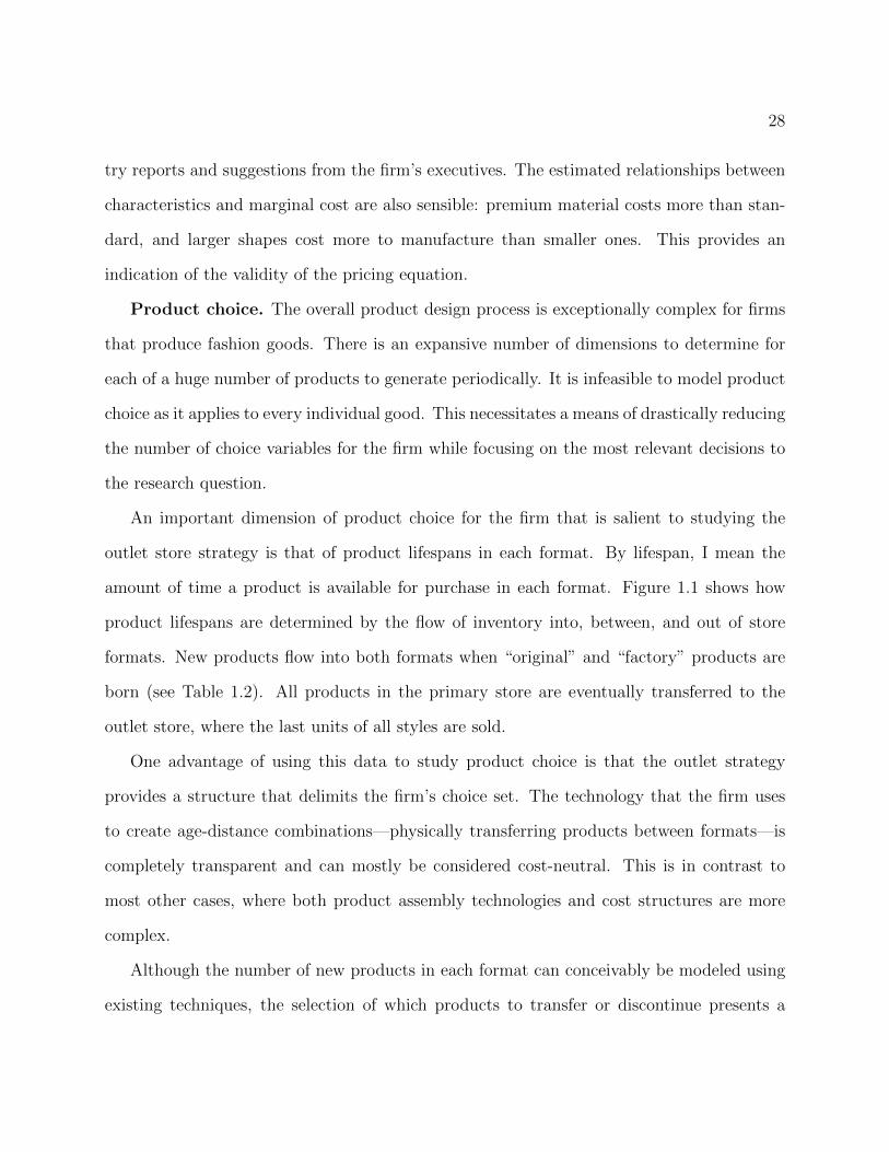
Product choice. The overall product design process is exceptionally complex for firms
that produce fashion goods. There is an expansive number of dimensions to determine for
each of a huge number of products to generate periodically. It is infeasible to model product
choice as it applies to every individual good. This necessitates a means of drastically reducing
the number of choice variables for the firm while focusing on the most relevant decisions to
the research question.
An important dimension of product choice for the firm that is salient to studying the
outlet store strategy is that of product lifespans in each format. By lifespan, I mean the
amount of time a product is available for purchase in each format. Figure 1.1 shows how
product lifespans are determined by the flow of inventory into, between, and out of store
formats. New products flow into both formats when “original” and “factory” products are
born (see Table 1.2). All products in the primary store are eventually transferred to the
outlet store, where the last units of all styles are sold.
One advantage of using this data to study product choice is that the outlet strategy
provides a structure that delimits the firm’s choice set. The technology that the firm uses
to create age-distance combinations—physically transferring products between formats—is
completely transparent and can mostly be considered cost-neutral. This is in contrast to
most other cases, where both product assembly technologies and cost structures are more
complex.
Although the number of new products in each format can conceivably be modeled using
existing techniques, the selection of which products to transfer or discontinue presents a

29
different challenge. Because the firm offers such a large number of products, an attractive
option is to think of the firm as targeting a joint probability of product characteristics rather
than individual product attributes. A primary contribution of this work is a demonstration
of this novel approach to modeling multidimensional product differentiation.
Specifically, I assume that store locations and capacities are given. Let Ck be the number
of items that store k can display on its shelves. I assume that in each period, each store k
takes Ck draws from a master set of products, represented by the distribution of product
characteristics h. Let h = f × g, where f is the joint distribution of endogenous product
characteristics (product ages by format) and g governs the set of exogenous characteristics
(summarized by ξj).4 The firm’s objective is to choose the profit-maximizing shape of f .
In order to make this problem tractable, I propose to construct f using a set of parametric
distributions. Industry logistics and the data suggest a natural choice for these distributions
and a direct interpretation of their parameters. Consider these assumptions on product
assortment:
1. The average original product in the primary format has a probability x of being trans-
ferred to discount in the next period.
2. The average factory product that is introduced in the outlet format has a probability
y of being retired in the next period.
3. The average original product that has been transferred to the outlet format has a
probability z of being retired in the next period.
4. The proportion of products in the outlet format that are factory goods is α.
These assumptions imply that if X is product age in the full-price format and Y is product
age in the discount format then
4Treating ξj as exogenous can be rationalized by the fact that the firm usually cannot ascertain the appealof a product to consumers until it is actually on shelves.

30
Figure 2.1: Empirical versus simulated age densities in primary format
X ∼ Geometric(x) (2.4)
Y =
W with probability α
X + Z with probability 1− α(2.5)
where W ∼ Geometric(y) and Z ∼ Geometric(z)
By adjusting the stopping probabilities x, y, and z, the firm can control the relative
distributions of product age in each store format. These probabilities also pin down the
portion of products that are new introductions in each period: the share of full-price products
that are newly introduced in a period is simply x and the share of new made-for-discount
products y. Figures 2.1 and 2.2 illustrates how closely this parameterization resembles the
observed distribution of product characteristics.
Products in the primary format, however, are not transferred to outlets at random.
Products that perform better in sales, and thus presumably are of higher quality, have
longer lifespans in primary stores. Figure C.3 plots the ξj against agej for the primary store
selections in the Indianapolis example from Figure 1.2. In the language of the exposition

31
Figure 2.2: Empirical versus simulated age densities in outlet format
above, the distribution of endogenous characteristics f is dependent on that of exogenous
characteristics g. I keep the form of this dependence fixed by allowing the firm to adjust the
speed of product turnover but not the order at which products are transferred according to
their ξj.
Clearly, adjusting the stocking probabilities, and thus the rate of new product introduc-
tions, is not cost-neutral. Assuming that the firm chooses to maintain a fixed number of
products in its universal offer set, the cost per period C(x, y) of implementing a given age
distribution must depend on the number of new product introductions it requires. I use the
simple cost function
C(x, y) = ax+ by (2.6)
to represent these costs.
To summarize, the firm chooses product choice parameters x, y, z, and α and prices p
to maximize expected profit

32
Figure 2.3: Better products are longer-lived in primary stores
E(π|x, y, z, α) =
∫ ∑m
Mm
∑j∈Jm
sj(pj −mcj)df(x, y, z, α)− C(x, y) (2.7)
In line with the earlier assumption that prices are profit-maximizing conditional on prod-
uct characteristics, I also assume that the firm chooses x and y optimally. This allows me
to identify cost parameters a and b exactly through the first order conditions of profit max-
imization: ∂E(π)/∂x = ∂E(π)/∂y = 0. I solve these equations numerically for a and b, and
present the implied product development costs in Table 2.1.
Note that this solution implies that the firm chooses its supply parameters once and for
all, precluding the possibility of making adjustments dynamically in response to demand
shocks. This simplifying assumption is made to keep the problem computationally feasible.
Conclusions drawn from counterfactuals performed in the next section pertain to static
results, and hence are robust to this assumption.

33
Before proceeding to discuss the fixed cost solutions, I describe how I compute the ex-
pected profit for perturbations around the observed x and y. First I sort the Ck products
according to age within each store k. This allows me to fix the dependence of the stocking
priorities on ξj. Given stocking probabilities x and y, I make ns sets of Ck draws from the
distributions specified in Equations 2.4 and 2.5.5 I replace the ages in the data with these
draws, keeping the original order according to age constant. I then compute the average over
corresponding profits for each of the ns draws.
Table 2.1: Implied product development costs
Product class Parameter Value Average stock Fixed cost per unit
Original (a) 7,779,203 151 51,518Factory (b) 19,034,202 433 43,959
The parameter values in Table 2.1 indicate the cost of replacing the entire stock of
products, i.e., when x = 1 or y = 1. Dividing these values by the average stock of each class
of product gives the fixed costs associated with developing each unit. I find that producing
each style of product carries a fixed cost of about $50,000, and that the fixed cost of producing
an original product is significantly higher than the fixed cost of a factory product.
With the model of price-setting and product introduction discussed in this section, to-
gether with the fixed and marginal costs that they imply, counterfactual store configurations
can now be properly evaluated.
2.3 Policy Simulations
The basic question that this chapter addresses is: Why do outlet stores exist? In this
section, I answer this question by simulating situations in which the firm pursues selling
5ns = 50 in this version.

34
strategies that exclude outlet store retail. For each of these policy simulations, I use the
supply-side model in Section 2.2 to specify how the firm would change its pricing and product
introduction rates in response to changes in store locations. The demand model from Chapter
1 then shows how consumers would react to these changes in firm strategy.
While the ideal exercise would be to generate optimal store locations in response to
changing demand conditions, such an endeavor would entail substantially more complex,
possibly infeasible, computation. Instead, I describe the shape of the firm’s objective function
by solving for optimal product assortment parameters given store locations. As such, the
results I derive are a conservative measure of the importance of the variables of interest.
Through the following counterfactuals, I find that outlet stores serve to expand the firm’s
market to include consumers who are more sensitive to prices, less averse to travel, and less
particular about product ages. Furthermore, the assortment in outlet stores is chosen to
prevent higher-value consumers from preferring to visit outlet stores over primary stores.
Test market. I use a representative market over which to perform policy simulations,
in order to clearly demonstrate the effects of each experiment. The test market is the
Indianapolis-Carmel Metropolitan Statistical Area in July 2007, maps of which were pre-
sented in Chapter 1. This market is representative of the firm’s markets both in terms of
the demand profile and the firm’s store and product configurations. Table 2.2 lists store
attributes and some performance measures in this market.
2.3.1 No outlet stores
The most natural policy experiment to perform involves simply removing the outlet store.
Many large retail firms choose not to operate outlet stores. Although a careful comparison
between firms is hard to make, it can be argued that these firms’ selling strategies are similar
to the firm’s primary store strategy taken alone in several respects. For instance, the current

35
Table 2.2: Test market store characteristics
Store: Primary 1 Primary 2 Outlet
Number of products 60 72 165Average price 313.46 329.39 154.28
Average product age (mo) 13.14 13.49 20.04Average distance (mi) 11.34 9.39 30.60
Units sold 148 217 967Revenue 29,861.96 50,083.60 119,057.12
firm’s primary stores are of similar size, configuration, and location to those of the second
biggest firm in the category, even though the other firm has no outlet stores.
Table 2.3 contains the results of this counterfactual as they pertain to the supply-side
responses. Column 1 contains the actual average prices, product ages, and revenues, which
are used as a baseline. Column 2 shows that revenues in primary stores increase when the
outlet store is closed, even when prices and assortment in the primary stores remain the
same. Column 3 shows that the firm would lower prices in primary stores in the absence
of outlet stores, even if it could not change the assortment (see Appendix B for details on
finding optimal prices). Column 4 shows that the firm would choose to make fewer product
introductions if outlet stores did not exist, resulting in an increase in average product age
in these stores.
The story is rounded out by looking at details of the demand-side response, which are
listed in Table 2.4. Closing the outlet store initially results in a very small increase in
primary store revenues because few of the consumers who shopped at the outlet store switch
to primary stores. When allowed to change product characteristics, the firm lowers quality
and price in the primary stores to cater to the lower-value consumers. However, even given
this flexibility, the firm is unable to serve the full range of consumers that it can with the

36
Table 2.3: No outlet stores (supply response)
1 2 3 4
Primary 1Price 313.46 313.46 280.21 220.73Age 13.14 13.14 13.14 15.12
Revenue 29,862 32,771 35,911 36,125
Primary 2Price 329.39 329.39 302.51 250.03Age 13.49 13.49 13.49 15.12
Revenue 50,084 55,831 62,200 67,830
OutletPrice 154.28 - - -Age 20.04 - - -
Revenue 119,057 - - -
Total revenue 199,003 88,602 98,111 103,955Variable profit 106,728 62,042 71,389 73,518
Prices and product ages are averages over each store.Columns indicate:1 - Baseline2 - Outlet store closed3 - Prices reoptimized4 - Prices and product ages reoptimized

37
outlet stores present.6
Table 2.4: No outlet stores (demand response)
1 2 3 4
Primary 1Distance aversion 73.98 70.04 65.32 63.42
Age aversion 45.17 42.99 39.13 35.16
Primary 2Distance aversion 81.09 80.82 72.15 70.21
Age aversion 42.65 41.53 37.26 32.88
OutletDistance aversion 32.55 - - -
Age aversion 25.90 - - -
Consumer values are averages over each store. Distanceaversion is the dollar equivalent to a consumer of a 20-mile increase in travel distance. Age aversion is equiv-alent to a 1-year increase in product age.Columns indicate:1 - Baseline2 - Outlet store closed3 - Prices reoptimized4 - Prices and product ages reoptimized
2.3.2 Random assortment
The assignment of products to either primary stores or outlet stores forms an important
part of the firm’s selling strategy. In this subsection, I show the value of the firm’s ob-
served assortment strategy by comparing its observed performance with that achieved by a
counterfactual assortment strategy in which products are randomly assigned to stores. This
random assignment results in a configuration in which primary and retail stores contain
6A clearer picture of which consumers are served can be presented through heat maps in consumer tastespace.

38
roughly identical assortments.7,8 This counterfactual strategy resembles that of firms that
open stores in outlet malls, but do not distinguish the assortment in these stores from those
in their non-outlet locations.
Table 2.5 describes the resulting average product characteristics in these stores. Here I
allow the firm to adjust prices, so that in both cases prices are profit-maximizing conditional
on product assortments. Jumbling the products results in near-identical average product
qualities between stores, but prices are still much lower in the outlet store. This suggests
that the bulk of discounting in outlet stores is to compensate for the inconvenience associated
with longer travel times.
Table 2.5: Randomized product distribution–supply
Assortment: Actual Randomized
Primary 1Age 13.14 16.92
Price 313.46 300.12Primary 2
Age 13.49 17.43Price 329.39 302.18
OutletAge 20.04 17.18
Price 154.28 170.48
As reported in Table 2.6, the firm’s performance suffers under a random assignment
of products to stores. Revenues in all stores decrease, and consumers are less different
between formats. This should be unsurprising, given that the products are less different
between formats. My hypothesis is that sorting works exceptionally well because there is
a positive correlation between consumer travel sensitivity and taste for newness. To test
7Recall that a product is unique only up to its fixed effect ξj , its price pjt, and its vintage agejt.
8Outlet stores will still have more shelf space than primary stores.

39
this hypothesis, I run the same counterfactual but under a supposed form of consumer
heterogeneity in which there is zero correlation between travel sensitivity and tastes for
newness.
Table 2.6: Randomized product distribution (actual tastes)
Assortment: Actual Randomized
Primary 1Distance aversion 73.98 70.87
Age aversion 45.17 41.74Primary 2
Distance aversion 81.09 75.42Age aversion 42.65 39.21
OutletDistance aversion 32.55 41.53
Age aversion 25.90 35.23
Total revenue 199,003 173,374Variable profit 106,728 85,150
Table 2.7 has the results of this experiment. As anticipated, randomizing assortment
has less of an effect when consumer tastes for the two attributes are uncorrelated. There
was little sorting to begin with, so the decrease does not come with very big a cost. This
result directly contradicts that of Armstrong and Rochet (1999). In their solution of a simple
model of multidimensional screening, they find that when consumer values for two product
attributes are highly correlated, the optimal menu features no dependence between the two
attributes. The authors point out in their paper that this result is counterintuitive; this
result confirms their intuition.
2.3.3 Centrally-located outlet stores
It seems plain to see that the firm pursues a “damaged goods” strategy by selling a portion
of its goods in distant locations. In order to confirm this hypothesis, I run a third set of

40
Table 2.7: Randomized product distribution (uncorrelated tastes)
Assortment: Actual Randomized
Primary 1Distance aversion 54.82 53.88
Age aversion 40.84 39.15Primary 2
Distance aversion 62.46 60.32Age aversion 37.28 36.71
OutletDistance aversion 41.38 43.28
Age aversion 31.84 33.18
Total revenue 153,432 151,883Variable profit 73,648 71,832
counterfactuals in which outlet stores are moved to central locations. I show that (i) revenues
decrease, (ii) the firm would make fewer product introductions in the outlet format, and (iii)
cater to a narrower range of consumers. I also show that the benefit of damaging goods in
this fashion is increasing in the taste correlation.
An alternative explanation to damaged goods is that firms locate in outlet malls to take
advantage of lower rents. Outlet malls on average set a monthly rent of $29.76 per square
foot, which can be dwarfed by rents in the most prestigious retail locations (Humphers 2012).
However, this rent is close to the average for retail space in many urban centers—implying
that the firm could choose to costlessly relocate its outlet stores closer to its target market.
Table 2.8 presents the supply-side results of the experiment in which the outlet store is
moved into the central shopping district. Notably, while prices are less variable now (primary
store products are cheaper and outlet store products are more expensive), quality along the
age dimension is more variable (primary store products are slightly newer and outlet store
products are much older). Denied the ability to differentiate products according to location,
the firm increases the level of differentiation according to age. The range of consumers that

41
the firm is able to reach, nevertheless, is similar to the case in which the outlet store is simply
shut down.
Table 2.8: Outlet moved to center (supply response)
Outlet location: Actual Central
Primary 1Age 13.14 12.78
Price 313.46 308.21Distance 11.34 11.34
Primary 2Age 13.49 13.00
Price 329.39 314.77Distance 9.39 9.39Outlet
Age 20.04 23.89Price 154.28 204.76
Distance 30.60 10.69
Total revenue 199,003 162,601Variable profit 106,728 70,419
Figure 2.4 shows the relationship between the relative profitability of outlet store retail
and the correlation between consumer tastes for quality and convenience. It is additional
evidence for the idea that the firm exploits the correlation in consumer attributes through its
outlet store strategy. It also suggests a plausible reason for why outlet stores have become
so popular among clothing and fashion firms, but not so much in other industries: tastes for
quality and convenience may not be so strongly correlated elsewhere.
These counterfactuals show that adding outlet stores helps the firm in many ways. First,
it extends the firm’s market to include consumers who are not averse to traveling and less
desirous of new things. Since these are the same people in the data, it makes sense for
the firm to populate its outlet stores with older products. This has the additional benefit
of making outlet store products less attractive to higher-value consumers, thus preventing

42
Figure 2.4: Central outlet policy vs taste correlation
cannibalization.
2.4 Conclusion
Owning and operating outlet stores constitutes a major component of many firms’ distri-
bution strategies, particularly in the clothing and fashion industries. It is an interesting
practice that continues to evolve and gain popularity. Yet there has been little written in
the marketing and economics literatures that speaks to the reasons for the success of outlet
stores, or the mechanisms by which they improve firm performance. The availability of new
sales data from a major fashion goods manufacturer and retailer offers a unique opportunity
to empirically investigate how outlet stores work.
This chapter shows that outlet stores provide several benefits as a tool of price discrimi-
nation. Outlet stores allow the firm to serve lower-value consumers without lowering prices
faced by its primary store clientele. By stocking outlet stores with less desirable products,

43
the firm exploits the positive correlation between consumers’ travel sensitivity and taste for
quality. Prices are low in outlet stores, but not low enough to attract consumers who value
quality and convenience the most.
The model of product choice in this essay suggests a benefit of running outlet stores apart
from its price discrimination uses: it allows the firm to make more frequent new product
introductions in its primary format. The firm offers more new products every period in its
primary stores both to increase the attractiveness of primary store offerings relative to those
in outlet stores and because it stocks outlet stores with older, less attractive products from
the primary stores. This can conceivably counter the threat that is most associated with
outlet stores: that it results in the dilution of prestige brands. Outlet stores may actually
enable the firm to improve its primary store products, which typically form the basis of a
fashion brand’s image.
Lessons from outlet store retail have wide applicability to questions of product line design
and price discrimination. Outlet stores are a specific response to the apparent heterogeneity
in tastes for quality and convenience among fashion shoppers. Similar responses by firms to
consumer tastes can be observed in the electronics and travel industries. The notion that
the correlation of characteristics in a firm’s product space ought to resemble the correlation
of consumer tastes for them may be useful to many firms.
The key insight is that multidimensionality in consumer preference heterogeneity matters
for product line design. Firms that seek to optimize their product offerings must take into
account how tastes vary for different product characteristics, and what the correlations
between those tastes are. This is not a new discovery: the extant theoretical literature on
multidimensional screening emphasizes the sensitivity of the optimal allocation set by the
principal to the agent’s value correlations. This is, however, the first demonstration of its
importance in an actual business setting. The choice of whether to operate outlet stores

44
hinges on a market landscape in which consumers who are most willing to travel to outlet
malls value quality the least.
There are many possible directions for future research. Outlet stores constitute a single
aspect of a consolidated selling strategy that has become standard among fashion goods
firms. Other parts of this strategy include price skimming, targeted coupons, and loyalty
programs. Many of these components operate on the intertemporal dimension of durable
goods demand. It would be interesting to see how they build on the firm’s overall product
lining strategy by adding yet additional dimensions.
This setting is also a prime vehicle for exploring alternative theories of consumer behavior
with respect to fashion goods demand. Consumers, for instance, may conceivably choose
products based on their capacity to signal status. Meanwhile, fashion goods may have
characteristics that are discernible to some consumers but not others (for instance, whether
a product is sold exclusively in outlet stores). This presents a unique product design challenge
to firms that wish to exploit these consumer preferences.

Chapter 3
Discount Pricing in Retail

46
3.1 Introduction
Firms often engage in discount pricing, in which prices are listed as a discount from an
original price. There are several reasons for which firms might drop the price of a good over
time, such as when it seeks to discriminate between consumers according to their willingness
to pay, as a means of managing its inventory, or when it faces less demand uncertainty after
the good’s introductory phase. In many of these instances, consumers can be thought of as
having nearly full information and making rational responses to price incentives. This essay,
on the other hand, focuses on motivations for discount pricing that arise from consumers
having imperfect information, or exhibiting irrational behavior. These are motivations that
might encourage firms to post high “original” prices at which products are never actually
available for purchase.
In this chapter, I identify patterns in how consumers respond to discounts. I use data
from a dominant fashion goods retailer that makes heavy use of this strategy in its outlet
stores. This data set offers a rare opportunity to study this pricing strategy because it
records both original and transacted prices, as well as repeat purchases. A portion of these
original prices are observably genuine, while the remainder are suggested. As with most
outlet stores, the firm implements random discounts across both time and products in store,
providing much variation in the transacted prices.
I find that consumer responses to suggested prices are consistent with several theories
both of prices as a signal of quality and of reference-dependent behavior. Controlling for
transactional prices and other product characteristics, a higher “original” price increases a
good’s purchase probability. While this effect is larger for products for which original prices
are genuine, it is also substantial for products with suggested original prices. Moreover, this
effect seems to be invariant to the consumer’s level of information.

47
Somewhat puzzlingly, this positive effect increases exponentially in the original price
(and equivalently, the discount amount). One might expect this effect to exhibit diminishing
marginal returns if consumers are less likely to put much stock in overly inflated original
prices. In addition, optimal behavior by firms would suggest concave returns to higher
suggested prices since increasing these prices is costless. I find that reference dependence
offers a partial explanation of this phenomenon. Consumers take the average discount level
in a store as the reference point, and are more likely to purchase goods that are more highly
discounted than this benchmark.
This reference dependence is in line with the idea that firms exploit bargain-hunting
behavior through suggested pricing. This effect may be particularly potent in outlet stores,
in which most items are discounted. Yet the attractiveness of a bargain must go hand-in-
hand with original prices being a reliable signal of quality. This implies that the firm must
maintain the credibility of these prices even as it employs them to manipulate consumer
behavior.
Setting suggested prices is a unique problem for the firm, as suggested prices can be
thought of as a signal of quality akin to certain forms of advertising. Yet unlike advertising,
setting higher suggested prices is costless to the firm. Setting optimal suggested prices,
therefore, involves balancing their (initially) demand-enhancing effects versus the possibility
that consumers may eventually lend less credibility to these signals.
This chapter proceeds as follows. Section 3.2 reviews the related literatures on pricing
and reference dependence. Section 3.3 describes the data used for the empirical analysis
and provides some descriptive statistics. Section 3.4 outlines a demand model and presents
parameter estimates. Section 3.5 concludes and points to directions for future work.

48
3.2 Related literature
Suggested pricing can occur in a wide variety of circumstances. The environment I consider
has the following features: a single seller that produces goods of varying quality, a weak
regulatory environment, consumers that have less information than the firm about prod-
uct quality and past prices, and the possibility of repeat purchases. An additional, novel
characteristic is that the marginal cost of production may not be monotonically increasing
with quality. This occurs, for instance, in the manufacture of fashion goods for which the
attractiveness of the final product may have little relationship with the processes involved
in its production.
Several authors have recognized the importance of price as a signal of quality for unin-
formed consumers. Bagwell and Riordan (1991) argue that high and declining prices can
indicate that a product is of high quality. In their framework, high prices are a credible
signal of quality because high quality, high-cost firms are more willing to restrict sales vol-
ume than low-cost firms. Over time, as the proportion of uninformed consumers decreases,
it becomes easier for the high-cost firm to signal its quality and thus its price lowers toward
the full-information monopoly price.
Armstrong and Chen (2013) examine a similar environment, but one in which quality is
endogenously determined and consumers can potentially be misled by false price announce-
ments. They find that when consumers are ignorant of the initial price, the firm finds it
profitable to produce a high quality good and announce the initial price when it is con-
strained to tell the truth. However, it does even better by producing a low quality good, and
subsequently misleading consumers by announcing a high initial price. Therefore, a key em-
pirical question of particular interest to regulators is: Are consumers deceived by suggested
prices?

49
Results from behavioral economics provide additional and alternative explanations for
why high suggested prices might be effective in driving demand. Bordalo, Gennaioli and
Shleifer (2013) argue that salient attributes are overweighted by consumers when choosing
between goods. They proceed to show how this logic can explain “misleading sales,” which
are mostly identical to what I term suggested pricing. The difference is that retailers inflate
original prices during misleading sales, instead of maintaining the same false original price
throughout a product’s lifetime.
Recently authors have begun to reconcile anomalous patterns in field data using concepts
generated in behavioral economics. One such example is Hastings and Shapiro (2012), who
find that consumers switch from premium to regular gasoline given a uniform price increase
to an extent that cannot be accounted for by wealth effects. They present this as evidence
of mental accounting, which manifests itself through the infungibility of money between an
individual’s different purposes (Thaler 1985).
The above-mentioned theories frequently have conflicting predictions on both consumer
behavior and firm decisions, owing to difference in fundamental assumptions. Perhaps be-
cause of the rareness of obtaining data with suggested prices, there has been no related
empirical work on actual retail settings. Thus, this is a valuable opportunity to test and
measure the relative importance of analytic results on both discount pricing and suggested
pricing.
Models of price as a signal of quality and those of reference dependence have different
predictions of how consumers react to false list prices and provide different motivations for
the firm to post suggested prices. Following Bagwell & Riordan (1991) and Armstrong &
Chen (2013), suppose that a monopolist supplies one good over two periods, setting prices
pt for periods t = 1, 2. Quality may be high or low, with marginal costs being ci, i ∈ {H,L}
respectively. Marginal costs are common knowledge. Consumers are heterogeneous in their

50
patience and there level of information about the quality of the good. A portion x of
consumers are trendy : they are eager to buy the good, can ascertain its quality, and are
in the market in period 1. The remaining 1 − x of consumers are casual : buyers who are
uncertain about the good’s quality and enter the market in period 2.
In Bagwell & Riordan (1991), casual consumers do not observe the purchasing decisions
of trendy consumers, and the firm is constrained to set p1 = p2. Casual consumers infer
product quality from price, their knowledge of the firm’s cost function and the proportion of
trendy consumers. If x is small enough, and under equilibrium refinements, casual consumers
accept a high price as a credible signal of high quality. Over time, as x increases, the firm
can signal high quality with less effort, and thus high quality goods exhibit prices that are
initially high but decline over time.
Armstrong & Chen (2013) relax the problem along several dimensions. First, the firm
is allowed to choose quality and set p1 6= p2. They show that if x is large enough, then the
firm chooses to provide high quality and set high prices in both periods if casual consumers
do not observe p1. The condition on x weakens when casual consumer can observe p1, which
provides an incentive for the firm to (credibly) inform casual consumers about past prices.
However, when casual consumers can be fooled into believing a false announcement about
p1, then the firm maximizes its profits by producing low quality goods, setting low prices in
period 1, and misinforming casual consumers about p1.
An alternative explanation of why suggested prices exist is provided by Bordalo et al.
(2013). They conceptualize salience as it applies to a discrete choice setting. Suppose the
consumer’s choice set is C ≡ (qj, pj)j=1,...,N . Each good j has quality qj and price pj. Without
salience effects, a consumers values good j with a utility function that assigns equal weights
to quality and price:
uj = qj − pj.

51
Salient thinking, meanwhile, puts more weight on attributes that stand out for each
good. Denote by (q, p) the reference good consisting of average attributes q =≡∑
j qj/N
and p =≡∑
j pj/N . The salience of quality for good j is then σ(qj, q) and the salience of
price is σ(pj, p).
The salience function σ(·, ·) is symmetric and continuous and satisfies the following con-
ditions:
1. Ordering. Let µ = sgn(aj − a). Then for any ε, ε′ ≥ 0 with ε+ ε′ > 0, we have
σ(aj + µε, a− µε′) > σ(aj, a).
2. Diminishing sensitivity. For any aj, a ≥ 0 and all ε > 0, we have
σ(aj + ε, a+ ε) < σ(aj, a).
In choice set C, quality is salient for good j when σ(qj, q) > σ(pj, p), price is salient
for good j when σ(qj, q) < σ(pj < p), and price and quality are equally salient when
σ(qj, q) = σ(pj, p).
An example of a salience function is
σ(aj, a) =|aj − a|aj + a
(3.1)
for aj, a 6= 0, and σ(0, 0) = 0.1
(Bordalo et al, 2013) The salient thinker’s evaluation of good j enhances the relative
utility weight attached to the salient attribute (keeping constant the sum of weights attached
1This function is also homogeneous of degree 0, which implies diminishing sensitivity.

52
to quality and price). Formally,
uSj =
2
1+δ· qj + 2δ
1+δ· pj if σ(qj, q) > σ(pj, p)
2δ1+δ· qj + 2
1+δ· pj if σ(qj, q) < σ(pj, p)
qj − pj if σ(qj, q) = σ(pj, p)
where δ ∈ (0, 1] decreases in the severity of salient thinking.
Using the definitions in this subsection I illustrate how a demand model that incorporates
salient thinking would predict different purchase decisions from a standard demand model.
Let C1 = {(q0 = 0, p0 = 0), (q1 = 15, p1 = 3), (q2 = 20, p2 = 4)}. A non-salient thinker
would assign values u1 = 12 and u2 = 16, and would thus opt for the high-quality product.
Applying the salience function in Eq. 3.1, quality and price are equally salient for both
goods, and thus a salient thinker would also opt for high quality.
Now consider a uniform price decrease so that C2 = {(q0 = 0, p0 = 0), (q1 = 15, p1 =
2), (q2 = 20, p2 = 3)}. Since utility is linear in quality and price, a non-salient thinker would
still choose the high quality product. However, quality is now salient for good 1 and price is
salient for good 2. Some algebra shows that a salient thinker would opt for the low quality
good if δ < 0.82.
Finally, we account for price expectations. Price expectations affect salience rankings by
influencing the reference good. The reference price is now taken by averaging transactional
together with expected prices. Taking expected prices as p1 = 3 and p2 = 4, quality becomes
salient for both goods in C2, so that the salient thinker continues to opt for the high quality
good for any δ ∈ (0, 1].
Thus, emphasizing the importance of salience in consumer decision-making, as well as
the primacy of price expectations, results in different predictions for how a firm should
apply suggested pricing in retail environments. At a basic level, the relevance of these

53
competing theories (price as a signal of quality versus salience) can be compared by examining
how consumers react to suggested prices, and measuring how this depends on consumer
characteristics and the choice sets.
3.3 Data and industry background
Data is provided by a major fashion goods manufacturer and retailer in the United States.
The firm sells above 90% of its products by revenue through its own physical stores. The
firm derives more than 60% of its revenue from a single product type, which is a fashion
good. All of the data and analysis in this chapter concerns this single product category. The
firm dominates as a market leader in this category, controlling about 40% of the market.
The firm operates two types of stores: regular and outlet. Regular stores are centrally
located and do not typically offer discounts on products. Outlet stores are typically located
an hour away from city centers and offer deep discounts (both actual and suggested). The
firm offers two main types of goods: original and factory. Original goods are first sold at
full price in regular stores and then sold at a discount in outlet stores. Factory goods are
only sold in outlet stores. The firm implements suggested pricing through its factory goods,
which carry original prices that are never transacted.
The data consists of transaction-level records over a 5-year period. Each record has the
original price of each item and any applied discount. Also included are consumer observables,
including billing zip code, date of first purchase from the firm, and household ID.
Consumers. Repeat purchases by consumers are observable in the data. A total of
16,019,140 unique consumers are observed to make purchases within the sample. The pro-
portion of purchases that are made by return consumers is significant (see Figure 3.1). In
the firm’s outlet channel, 24% of purchases are made by return consumers. Of this group,

54
Figure 3.1: Consumers by number of within-sample purchase instances
38% have made purchases in the regular channel.
Prices. Table 3.1 describes the pricing differences between original and factory goods
in outlet stores. Original goods are more expensive than factory goods on average, both in
terms of list prices and transactional prices. However, there is much variation in these prices
over time; and factory goods occasionally carry higher prices than original goods (see Figure
C.4).
Figure 3.2 graphs the average percent discount over time for original goods and factory
goods in the firm’s outlet channel. Recall that original goods are sold at full price in the
regular channel, while factory goods are sold exclusively in the outlet channel. The similar
trend in discount increase over time for these two product classes reflects the firm’s policy of
trimming prices at even rates across all products over time, regardless of sales performance.

55
Table 3.1: Average prices in outlet format
Original goods Factory goods
List price 349.03 308.87[177.45] [85.50]
Discount percent 50.84 58.90[13.81] [11.74]
Transactional price 165.76 123.20[85.82] [38.03]
On-shelf composition 69.64% 30.36%
Revenue composition 30.90% 69.10%
Figure 3.2: Discounting pattern in outlet channel

56
Figure 3.3: Discounting pattern of a typical good
The pattern of discounting implemented by the firm in its outlet stores has store, pe-
riod, and product-specific components. Across stores and time periods, the firm implements
randomized discounting within certain parameters. Occasionally these discounts are also
affected by outlet mall-wide events. The product-specific component of discounting is highly
correlated with the product’s design age, i.e. the time since its introduction. Older-lived
products are discounted more heavily. Figure 3.3 plots the list price and observed transac-
tional prices for a single factory good over time, displaying the resulting discount pattern
for a typical product.
The red line on Figure 3.3 marks the original price assigned to this particular product.
Every single purchase instance over the product’s lifetime is plotted on the graph; obviously
not a single unit was sold anywhere near the original price. Not immediately observable

57
from the graph is that 94% of units were sold by the end of 2008. This is consistent with
high consumer values for a product’s newness in this industry. The remaining purchase
observations show that the firm does not use discounting in order to clear inventory.
Figure C.2 in the appendix shows that the firm has increased the average discount level
over time. This shift provides an opportunity to study the effect on purchase decisions
of discount pricing. It also demands an explanation as to why such a pricing strategy is
effective.
3.4 Demand model
In this section I present a discrete choice model of consumer purchase behavior and estimate
its parameters using data from a major fashion goods retailer. The main objective of estima-
tion is to verify that list prices affect purchase behavior keeping all other product attributes,
including the actual selling price, constant. I measure how this effect varies across consumer
types. I proceed to decompose consumer sensitivity to different components and ranges of
discounting in order to identify the margins in which suggested pricing is most effective.
Finally, I test for the significance of certain reference points that may influence the salience
of discounting.
The model presented below differs slightly from the demand model estimated in Chapter
1. The first main difference is that instead of including both store and product choice, the
model below concerns only product choice conditional on store choice. The rationale for this
focus is that discount pricing is exercised most heavily in the outlet channel. Additionally,
this allows me to use store foot traffic as a measure of market size. The second main difference
is that, rather than estimating product fixed effects, I include product characteristics in the
utility function. This is necessary given that there is no within-product variation in list

58
prices.
Let product j in store m and time t be defined by observable characteristics Xjt, unob-
served quality ξj, list price LPj, and transactional price pjmt. The utility of consumer i from
purchasing product j in market m is
uijmt = αpjmt +Xjtβ + γLPj + ξj + εijmt (3.2)
where α, β, and γ, are parameters, and εijmt are idiosyncratic demand shocks. (Allowing for
greater consumer heterogeneity is left for future work. In what follows the model is estimated
within subsets of the data, which is indicative of the importance of consumer heterogeneity.)
Letting εijmt be iid Type-I extreme value, and inverting the resulting system of market
share equations (Berry 1994), we have that mean utilities can be written as
log(sjmt)− log(s0mt) = δjmt ≡ αpjmt +Xjtβ + γLPj + ξj
where sjmt are market shares and s0mt is the share of the outside good. A consumer is
considered to have chosen the outside good if she has visited a store but has not made a
purchase. Availability of foot traffic counts for each store-week enables direct observation of
these outside shares.
Initial estimation of demand parameters is by OLS regression of mean utility levels on
observables. A market is defined as a store-week. The market size is taken to be the foot
traffic recorded in each store-week. Product characteristics Xjt include product age and
categorical variables relating to shape, color, material, and collection.2 Store and week fixed
effects are also included. Descriptive statistics for these variables in the estimation sample
2A collection is a set of products that share the same general aesthetic. Products are presented in shelvesaccording to their collection in the firm’s regular channel. In the firm’s outlet channel, products are groupedaccording to other physical characteristics.

59
are reported in Table 3.2.3
Table 3.2: Sample descriptive statistics
Mean St. Dev. Count
Market size 9303.74 6442.74 Stores 124Market share 0.00074 0.00065 Weeks 27Price 120.80 32.84 Colors 350List price 337.73 63.37 Materials 29Age (days) 305.30 152.74 Silhouettes 20Factory 0.89 0.31 Collections 47
Estimates from the OLS regression are reported in column 1 of Table 3.3. Dummies
for each categorical variable, as well as for stores and weeks, are included in this and all
succeeding regressions. As anticipated, purchase probability is positively correlated with
original price, and negatively with the product’s design age. However, these estimates are
likely biased and inconsistent owing to a dependence of pjmt and LPj on ξj.
As discussed in previous chapters, the general level of pjmt is determined via a national
pricing strategy. Within-product variation in pjmt arises from randomized experiments un-
dertaken by the firm in order to gauge the effectiveness of planned promotions, as well as by
a systematic decline over product age as summarized in Table 1.6. Therefore, any correlation
between pjmt and ξj must follow the same mechanism as that between LPj and ξj.
Instruments for pjmt comprise the average discount percent in a store-week, selected
collection dummies, and their interactions. The average discount percent in a store-week
reflects store- instead of product-specific departures from full price, and are assumed to
be uncorrelated with ξj. The collection to which a product belongs may be a suitable
instrument because while pjmt and LPj are highly correlated with collection (see Table
C.3), most collections themselves have no bearing on product quality controlling for physical
3In this version, the estimation sample includes 27 weeks and 124 stores.

60
Table 3.3: Demand estimates
(1) (2)dep var: δjmt OLS IV
actual price -0.00788*** -0.0108***[5.05e-05] [0.000119]
list price 0.00118*** 0.00198***[2.73e-05] [7.44e-05]
product age -0.000166*** -0.000297***[1.05e-05] [1.17e-05]
factory -0.194*** -0.289***[0.00841] [0.00918]
constant -5.855*** -5.815***[0.512] [0.514]
Observations 429,730 429,730R-squared 0.536 0.532
Standard errors in brackets*** p<0.01, ** p<0.05, * p<0.1
characteristics.
Instruments for LPj are constructed from list prices of products in the same collection
as product j but in other categories. The operative assumption is that, while the relative
magnitude of list prices are largely determined by collection across product categories, there
is no relationship between the unobserved quality of the main product category and that of
list prices of products in other categories within the same collection.
From the total number of collections, I select the most prominently advertised and widely
purchased collections as regressors in the second stage, and use the remaining collections as
instruments in the first stage. The reasoning is that, apart from the most popular among
them, collections in the outlet channel mainly serve as record-keeping devices for the firm,
that while related to pricing, are difficult for consumers to distinguish.
As a means of verifying that this subset of product collections are valid instruments,

61
I estimate product intercepts for each of the 3,360 unique styles in the sample using this
alternative demand model:
uijmt = αpjmt + ξj + εijmt
Figure C.3 in the appendix plots the estimated ξj against LPj. I assume that ξj incor-
porates both observed and unobserved components of quality. I project ξj on regressors Xj,
excluding collection dummies, and LPj and collect the residuals. These residuals, then, com-
prise the unobserved component of quality. I regress the residuals on collection dummies,
and select the 42 collections for which t-stat is less than 2 as instruments for LPj in the main
model. The results of the IV estimation are in column 2 of Table 3.3.
Instrumenting for LPj eliminates the bias resulting from objectively higher quality prod-
ucts having higher original prices; the magnitude of the IV estimate suggests a large scope
for LPj’s influence on purchase behavior controlling for actual product quality. The esti-
mated price coefficient in Table 3.3 implies an average price elasticity of 1.24. Comparing
coefficients suggests that each dollar reduction in transactional price has about the same
effect on utility as a $5-6 dollar increase in list price.
This simple demand model implies that consumers consider list prices when making their
purchase decisions, but does not offer an interpretation as to why consumers do so. Possible
reasons are that (i) consumers delay purchases to take advantage of discounts, (ii) consumers
take list prices as a signal of quality, (iii) consumers enjoy receiving discounts, or (iv) the
firm more aggressively markets products with deeper discounts. Each of these hypotheses,
if valid, would correspond to certain patterns in purchase behavior. In the remainder of this
section, I extend the basic demand model from Equation 3.2 to verify if these patterns exist
in the data.

62
Price as a signal of quality. Consumers who lack full information may take price as
a signal of quality. Demand data, coupled with transactional and list prices, offer an oppor-
tunity to measure this signaling effect separately from the more common price sensitivity. If
less-informed consumers are more reliant on this signal, then they should demonstrate more
sensitivity to list prices.
To check whether this holds true in the data, I bucket the purchase observations according
to first-time and repeat consumers.4 The assumption is that repeat consumers are better
informed about product quality owing to their greater experience with the brand. I estimate
the regression model for each bucket and present the results in Table 3.4. The estimates
suggest that repeat consumers are in fact more sensitive to list prices. This runs counter
to the underlying assumptions of signaling models, suggesting that either the evolution of
consumer information or the role of list prices is more complex.
Alternatively, I limit the sample to include only old consumers, and then divide the
sample according to consumers who have visited the regular store in the past and those
that haven’t. The corresponding estimates are reported in Table 3.5. Strikingly, although
full-price shoppers are much less (transactional) price sensitive than pure factory shoppers,
they share almost the same sensitivity to LPj.
An important distinction exists between original and factory goods in this market. Orig-
inal goods are those that were previously sold in the firm’s regular channel at their original
prices. Factory goods are those that were never sold in the regular channel, but are tagged
with suggested prices. Consumers in this market vary in their ability to distinguish original
from factory goods. Presumably consumers who have shopped in the regular channel in the
past are more able to make this distinction. Table 3.6 contains the estimated coefficient
4Unfortunately outside shares cannot be directly bucketed in the same way. I take the ratio of purchasesof minor product categories and apply them to the outside shares for estimation purposes.

63
Table 3.4: New vs old consumers
(1) (2)First-time consumers Old consumers
pj -0.00689*** -0.00657***[0.000134] [8.45e-05]
LPj 0.000582*** 0.000770***[8.21e-05] [4.78e-05]
age 4.83e-05*** -2.06e-05***[1.08e-05] [1.45e-05]
factory -0.122*** -0.119***[0.0193] [0.00756]
constant -6.195*** -8.253***[0.761] [0.287]
Observations 224,869 415,079R-squared 0.555 0.477
Standard errors in brackets*** p<0.01, ** p<0.05, * p<0.1
Table 3.5: Pure factory vs full price shoppers
(1) (2)Pure factory Full-price
pj -0.00611*** -0.00393***[9.54e-05] [0.000107]
LPj 0.000564*** 0.000541***[5.92e-05] [6.14e-05]
age -2.84e-05*** -3.08e-05***[1.01e-05] [1.09e-05]
factory -0.118*** -0.122***[0.00764] [0.00824]
constant -7.926*** -7.708***[0.176] [0.237]
Observations 302,778 179,929R-squared 0.501 0.595
Standard errors in brackets*** p<0.01, ** p<0.05, * p<0.1
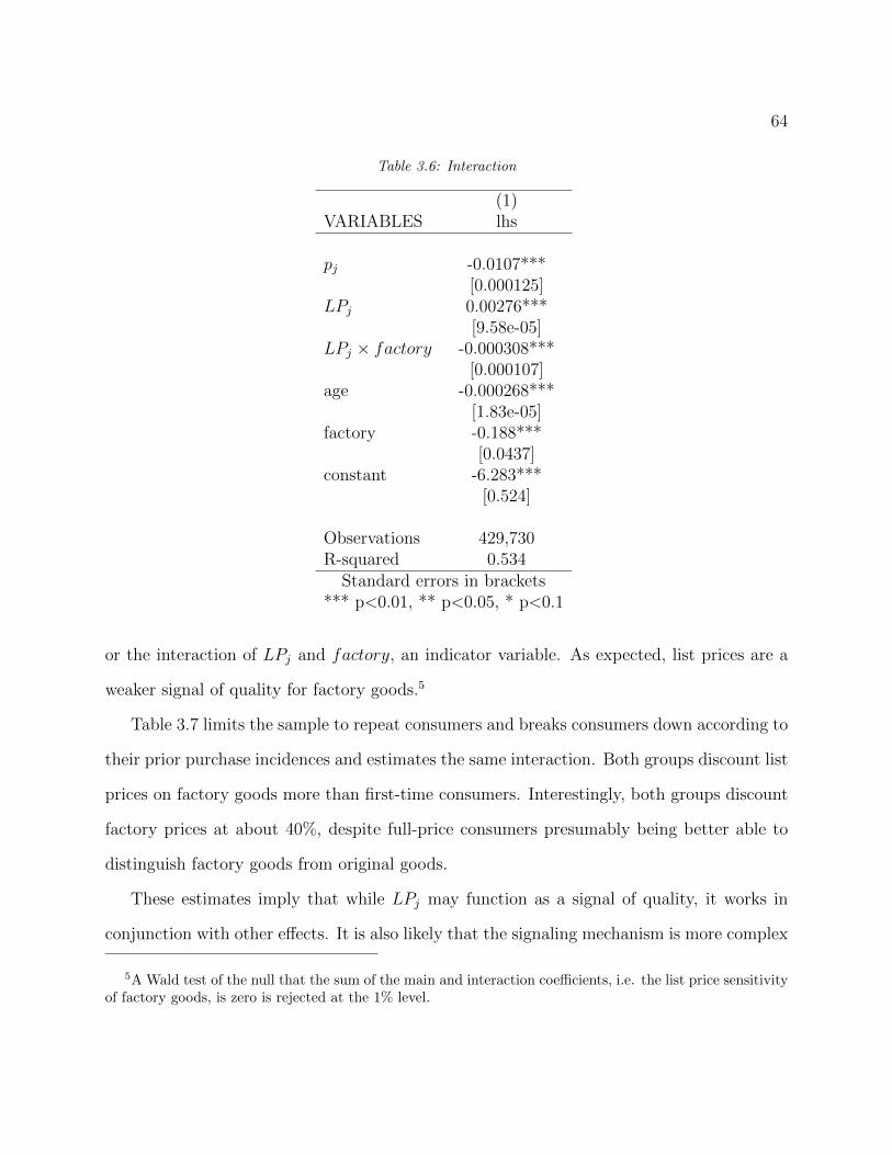
64
Table 3.6: Interaction
(1)VARIABLES lhs
pj -0.0107***[0.000125]
LPj 0.00276***[9.58e-05]
LPj × factory -0.000308***[0.000107]
age -0.000268***[1.83e-05]
factory -0.188***[0.0437]
constant -6.283***[0.524]
Observations 429,730R-squared 0.534
Standard errors in brackets*** p<0.01, ** p<0.05, * p<0.1
or the interaction of LPj and factory, an indicator variable. As expected, list prices are a
weaker signal of quality for factory goods.5
Table 3.7 limits the sample to repeat consumers and breaks consumers down according to
their prior purchase incidences and estimates the same interaction. Both groups discount list
prices on factory goods more than first-time consumers. Interestingly, both groups discount
factory prices at about 40%, despite full-price consumers presumably being better able to
distinguish factory goods from original goods.
These estimates imply that while LPj may function as a signal of quality, it works in
conjunction with other effects. It is also likely that the signaling mechanism is more complex
5A Wald test of the null that the sum of the main and interaction coefficients, i.e. the list price sensitivityof factory goods, is zero is rejected at the 1% level.

65
Table 3.7: Consumer sensitivity to list prices
(1) (2) (3) (4)Shopper type Discount Discount Full-price Full-price
pj -0.00792*** -0.00793*** -0.00624*** -0.00635***[8.89e-05] [8.25e-05] [0.000115] [0.000121]
LPj 0.00173*** 0.00278*** 0.00158*** 0.00189***[4.33e-05] [9.67e-05] [6.06e-05] [0.000147]
LPj × factory -0.000992*** -0.000485***[9.34e-05] [0.000134]
constant -9.004*** -9.136*** -7.432 -7.727[0.622] [0.624] [0.483] [0.498]
Observations 185,387 185,387 92,739 92,739R-squared 0.559 0.559 0.622 0.622
Standard errors in brackets*** p<0.01, ** p<0.05, * p<0.1
than what these simple demand models can capture. In what follows I include various
reference points to the consumer’s utility function in an effort to parse these effects without
adding complexity to the model.
Reference dependence. The potency of price as a signal of quality and the intensity
of bargain-hunting behavior are closely linked in this empirical setting. A discount is only
a genuine “deal” if the original price is a dependable measure of the product’s quality.
One way to distinguish between these effects is by incorporating reference dependence in
modeling consumer demand. The extent to which consumers respond to high original prices,
or equivalently high discounts, may depend on the general level of discounting, the dispersion
in discount levels, or some other reference point.
In what follows I focus on reference points that are specific to a store-week. The thinking
is that consumer values are swayed by product attributes’ relative distance to some reference
level, which in this case is most likely determined during their store visit. Table 3.8 lists

66
Table 3.8: Description of variable labels in Table 3.9
Model Regressor Definition1 discount original price less transactional price2 discount2 discount2
3 higher indicator for above-median discountdisc higher higher × discount
4 discz within-market z-score of discountdiscz disc discz × discount
5 posz positive z-scoresnegz negative z-scoresdisc pos discount × poszdisc neg discount × negz
6 avedisc average discount in marketsddisc st dev of discount in marketdisc ave discount × avediscdisc sd discount × sddisc
7 mindisc minimum discount in marketresid disc discount less mindisc
8 resid disc2 resid disc2
9 upper indicator for above-median resid discup resid resid disc × upper
10 residdiscz within-market z-score of resid discresiddiscz resid disc resid disc × residdiscz
11 rposz positive values of residdisczrnegz negative values of residdisczrdisc pos resid disc × rposzrdisc neg resid disc × rnegz
variables that may influence the relative attractiveness of discounts in-store. Table 3.9 con-
tains estimates for various specifications that include these variables. Most of the estimated
coefficients are large and significantly different from zero, implying considerable scope for
reference dependence to influence consumer choice.
The estimates support intuitive notions of reference dependence. The utility from a
discount is amplified if the discount is larger than the median level of discounting. In
specifications 7 through 11 of Table 3.9, the baseline minimum discount available in a store-

67
Tabl
e3.9
:R
efer
ence
poin
ts
(1)
(2)
(3)
(4)
(5)
(6)
(7)
(8)
(9)
(10)
(11)
price
-0.00639***
-0.00638***
-0.00635***
-0.00638***
-0.00638***
-0.00635***
-0.00636***
-0.00636***
-0.00635***
-0.00636***
-0.00635***
[4.03e-0
5]
[4.03e-0
5]
[4.04e-0
5]
[4.04e-0
5]
[4.04e-0
5]
[4.04e-0
5]
[4.03e-0
5]
[4.03e-0
5]
[4.04e-0
5]
[4.03e-0
5]
[4.04e-0
5]
age
-6.67e-0
5***
-6.02e-0
5***
-6.25e-0
5***
-6.19e-0
5***
-7.01e-0
5***
-6.84e-0
5***
-6.40e-0
5***
-6.01e-0
5***
-5.95e-0
5***
-6.18e-0
5***
-6.53e-0
5***
[1.15e-0
5]
[1.15e-0
5]
[1.15e-0
5]
[1.15e-0
5]
[1.16e-0
5]
[1.15e-0
5]
[1.15e-0
5]
[1.15e-0
5]
[1.15e-0
5]
[1.15e-0
5]
[1.16e-0
5]
facto
ry-0
.210***
-0.205***
-0.217***
-0.206***
-0.218***
-0.213***
-0.210***
-0.207***
-0.212***
-0.208***
-0.217***
[0.0113]
[0.0113]
[0.0114]
[0.0114]
[0.0114]
[0.0113]
[0.0113]
[0.0113]
[0.0113]
[0.0113]
[0.0114]
discount
0.00101***
0.000306***
2.35e-0
50.000927***
0.00125***
-0.00288***
[2.93e-0
5]
[9.33e-0
5]
[5.95e-0
5]
[0.000107]
[0.000111]
[0.000318]
discount2
1.36e-0
6***
[1.70e-0
7]
higher
-0.285***
[0.0142]
dischigher
0.00137***
[6.70e-0
5]
discz
-0.0137**
[0.00578]
disczdisc
6.21e-0
5***
[1.11e-0
5]
discpos
-5.91e-0
5***
[1.67e-0
5]
discneg
0.000461***
[5.91e-0
5]
posz
0.0215***
[0.00759]
negz
-0.104***
[0.0111]
discave
2.16e-0
5***
[1.25e-0
6]
discsd
-1.52e-0
5***
[2.22e-0
6]
avedisc
-0.00283***
[0.000315]
sddisc
0.00302***
[0.000514]
min
disc
0.00299***
0.00291***
0.00284***
0.00257***
0.00268***
[8.91e-0
5]
[9.05e-0
5]
[9.16e-0
5]
[0.000128]
[0.000130]
resid
disc
0.000996***
0.000738***
0.000467***
0.000520***
0.000753***
[2.93e-0
5]
[6.32e-0
5]
[5.99e-0
5]
[0.000111]
[0.000114]
resid
disc2
7.71e-0
7***
[1.67e-0
7]
up
resid
0.000730***
[6.90e-0
5]
upper
-0.0826***
[0.00841]
residdiscz
0.0170***
[0.00555]
residdisczre
sid
disc
4.53e-0
5***
[1.11e-0
5]
rdiscpos
-6.75e-0
5***
[1.66e-0
5]
rdiscneg
0.000160**
[6.25e-0
5]
rposz
0.0451***
[0.00643]
rnegz
-0.0179***
[0.00690]
Constant
-7.023***
-6.903***
-6.809***
-6.983***
-7.093***
-6.550***
-7.237***
-7.196***
-7.173***
-7.125***
-7.200***
[0.741]
[0.741]
[0.741]
[0.742]
[0.742]
[0.745]
[0.741]
[0.741]
[0.741]
[0.741]
[0.741]
Obse
rvations
429,730
429,730
429,730
429,727
429,727
429,727
429,730
429,730
429,730
429,727
429,727
R-square
d0.543
0.543
0.544
0.543
0.543
0.544
0.544
0.544
0.544
0.544
0.544
Sta
ndard
errors
inbra
ckets
***
p<0.01,**
p<0.05,*
p<0.1

68
week enters separately from each product’s residual discount. The estimated coefficient
for the baseline is about three times that for the residual, suggesting that market-wide
discounting is more effective at inducing purchases than product-specific discounting. A
possible reason for this is that steeper product-specific discounts may carry a negative signal
about a product’s popularity or earlier sales performance.
A look at the distribution of available discounts over time suggests that the firm has
been decreasing the dispersion of available discounts even as it increases the average (see
Figure C.1). At the same time, the firm has been decreasing the scope of product-specific
discounts relative to market-specific discounts. Given the results of demand estimation, one
interpretation is that the firm is taking advantage of demand-enhancing store-wide discounts,
while minimizing the role of product-specific discounts that carry negative signals about
product quality.
Intertemporal substitution. Consumers have been documented to time their pur-
chases to correspond with periodic promotions (e.g. Hendel & Nevo 2011) or to take ad-
vantage of declining prices over time (e.g. Nair 2007). I argue that the empirical setting in
this essay is not conducive to either of these substitution behaviors. Unlike those in grocery
stores, outlet store promotions are irregularly timed and difficult to schedule visits over (see
Figure C.2). Although the transactional price for each product does systematically decline
over time, so does the product’s inherent attractiveness as a fashion good.
I include past-period transactional price pj,t−1 in the regression equation to assess if
intertemporal substitution is in fact an important factor in purchase decisions. Controlling
for the current period’s price, the coefficient on the past period’s price should be positive if
consumers time their purchases to take advantage of lower prices. The estimated coefficient
turns out to be negative and statistically significant (see Table 3.10).
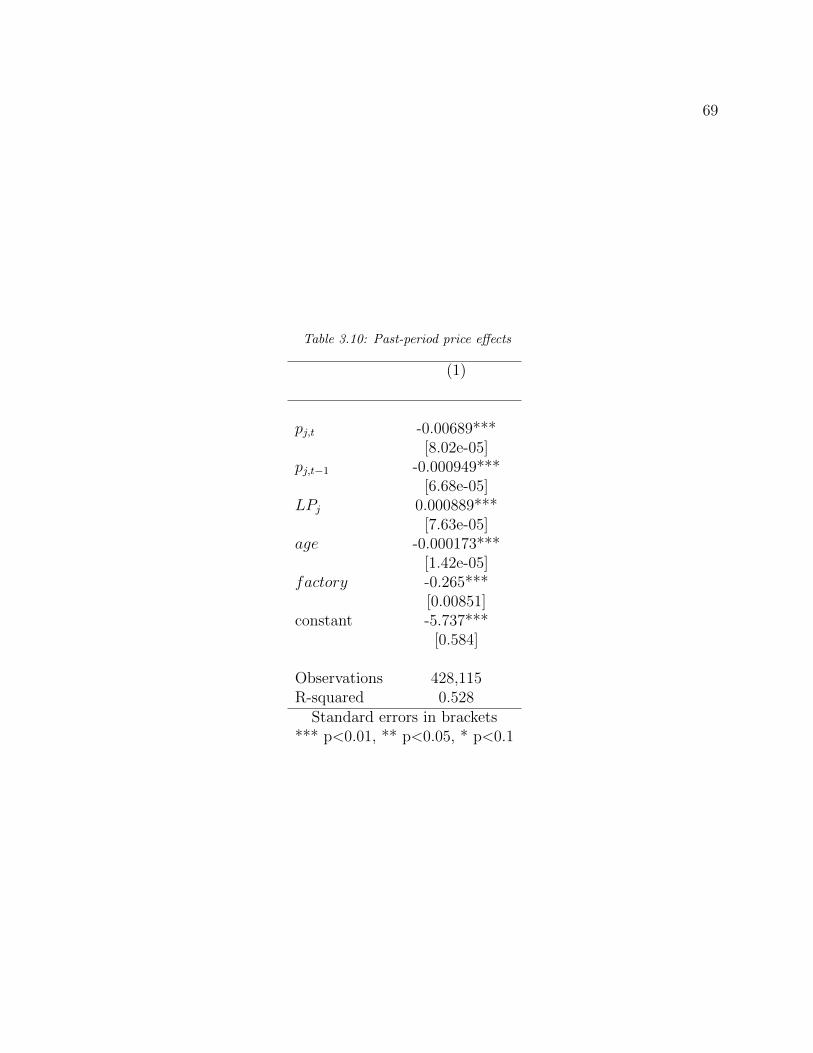
69
Table 3.10: Past-period price effects
(1)
pj,t -0.00689***[8.02e-05]
pj,t−1 -0.000949***[6.68e-05]
LPj 0.000889***[7.63e-05]
age -0.000173***[1.42e-05]
factory -0.265***[0.00851]
constant -5.737***[0.584]
Observations 428,115R-squared 0.528
Standard errors in brackets*** p<0.01, ** p<0.05, * p<0.1

70
3.5 Conclusion
Price comparisons, whether suggested or not, have become ubiquitous signals in retail set-
tings. The question of how these signals affect purchase behavior is relevant to firms, regula-
tors, and perhaps consumers themselves. Firms, in list prices, possess a potentially powerful
driver of demand that is virtually costless to produce and adjust. Regulators face the chal-
lenge of assessing whether list prices inform or deceive, and ultimately whether they enhance
or damage consumer welfare. Consumers may be surprised to find out how list prices are
determined, and the extent to which their own decisions are reliant on them.
This chapter shows that list prices have significant effects on purchase decisions that may
operate through several channels. On average, consumers may be thought of as assigning a
monetary value to list prices at over 20 actual cents to a suggested dollar. This rate seems
invariant to the consumer’s depth of experience with a brand.
In addition, values for discounts depend on market-specific reference points. For instance,
discount sensitivity is much higher at levels above the average discount in a market. Con-
sumers are also more sensitive to discounts where the variance of discounting is higher. These
suggest that optimal price-setting by the firm should incorporate reference dependence in
consumer behavior.
For future work, I plan on incorporating consumer heterogeneity in measuring the impact
of suggested pricing. Efforts at identifying the effect of heterogeneity in this chapter rely on
strong assumptions about how past shopping experience affects consumer information and
behavior. Relaxing these assumptions by allowing list price effects to vary flexibly may be
provide clues as to which consumer segments are most swayed by list prices.
I also plan to study how consumer behavior provides incentives for the firm to pursue a
strategy of setting suggested prices. Since this form of price-setting is costless to the firm,

71
there must be countervailing forces that make setting ever-higher suggested original prices
suboptimal. Identifying these countervailing forces is necessary to make the firm’s suggested
pricing optimization problem well-defined.
The existing literature on price as a signal of quality views suggested list prices only as
a means of deceiving uninformed consumers. This literature relies on the strictly monotonic
relationship of quality and marginal cost as providing credibility to actual selling price as a
signal of quality. In the future, I plan on developing a model in which quality is generated
through a stochastic process indexed by marginal cost, and exploring the role that list prices
can play in reducing asymmetric information about quality between the firm and consumers.
This is motivated by settings in which quality can only imperfectly be set by firms, such as
in fashion and design related industries.

Bibliography
[1] Armstrong, Mark. “Multiproduct nonlinear pricing.” Econometrica: Journal of the
Econometric Society (1996): 51-75.
[2] Armstrong, Mark, and Yongmin Chen. “Discount pricing.” Mimeo. (2012).
[3] Armstrong, Mark and Rochet, Jean-Charles. 1999. “Multi-dimensional Screening: A
User’s Guide. European Economic Review 43, 959-979.
[4] Bagwell, Kyle. “Pricing to signal product line quality.” Journal of Economics & Manage-
ment Strategy 1.1 (1992): 151-174.
[5] Bagwell, Kyle, and Michael H. Riordan. “High and declining prices signal product qual-
ity.” The American Economic Review (1991): 224-239.
[6] Bayus, Barry L., and William P. Putsis. 1999. “Product proliferation: An empirical
analysis of product line determinants and market outcomes.” Marketing Science 18.2:
137-153.
[7] Berry, Steven T. “Estimating discrete-choice models of product differentiation.” The
RAND Journal of Economics (1994): 242-262.
[8] Berry, Steven, James Levinsohn, and Ariel Pakes. “Automobile prices in market equilib-
rium.” Econometrica: Journal of the Econometric Society (1995): 841-890.72

73
[9] Blair, Edward A., and E. Laird Landon Jr. “The Effects of Reference Prices in Retail
Advertisements.” Journal of Marketing 45.2 (1981).
[10] Bordalo, Pedro, Gennaioli, Nicola, and Andrei Shleifer. “Salience and consumer choice.”
The Journal of Political Economy (2013): 803-843.
[11] Chen, Yongmin and Riordan, Michael H. 2012. “Profitability of Product Bundling.”
Mimeo, Columbia University.
[12] Coughlan, Anne T. and Soberman, David. 2005. “Strategic Segmentation Using Outlet
Malls.” International Journal of Research in Marketing 22, 61-86.
[13] Crawford, Gregory. 2012. “Endogenous Product Choice: A Progress Report.” Interna-
tional Journal of Industrial Organization 30, 315-320.
[14] Crawford, Gregory S., Oleksandr Shcherbakov, and Matthew Shum. “The welfare effects
of monopoly quality choice: Evidence from cable television markets.” Unpublished paper
(2011).
[15] Deneckere, Raymond J., and R. Preston McAfee. “Damaged goods.” Journal of Eco-
nomics & Management Strategy 5.2 (1996): 149-174.
[16] Desai, Preyas S. “Quality segmentation in spatial markets: When does cannibalization
affect product line design?.” Marketing Science 20.3 (2001): 265-283.
[17] Dobson, Gregory, and Shlomo Kalish. “Positioning and pricing a product line.” Mar-
keting Science 7.2 (1988): 107-125.
[18] Dolan, Maura. “Kohl’s can be sued over sale ads, court says.” Los Angeles Times. May
22, 2013.

74
[19] Draganska, Michaela, and Dipak C. Jain. “Consumer preferences and product-line pric-
ing strategies: An empirical analysis.” Marketing Science 25.2 (2006): 164-174.
[20] Draganska, Michaela, Michael Mazzeo, and Katja Seim. “Beyond plain vanilla: Model-
ing joint product assortment and pricing decisions.” QME 7.2 (2009): 105-146.
[21] Fan, Ying. “Ownership consolidation and product quality: A study of the us daily
newspaper market.” Working Paper, University of Michigan, 2010.
[22] Green, Paul E., and Abba M. Krieger. 1985. “Models and heuristics for product line
selection.” Marketing Science 4.1: 1-19.
[23] Harkrader, Carleton A. “Fictitious Pricing and the FTC: A New Look at an Old Dodge.”
St. John’s L. Rev. 37 (1962): 1.
[24] Hastings, Justine, and Jesse M. Shapiro. Mental accounting and consumer choice: Evi-
dence from commodity price shocks. No. w18248. National Bureau of Economic Research,
2012.
[25] Heiss, Florian, and Viktor Winschel. “Likelihood approximation by numerical integra-
tion on sparse grids.” Journal of Econometrics 144.1 (2008): 62-80.
[26] Hendel, Igal, and Aviv Nevo. Intertemporal price discrimination in storable goods mar-
kets. No. w16988. National Bureau of Economic Research, 2011.
[27] Humphers, Linda. 2012. “State of the Outlet Industry.” Value Retail News.
[28] Johnson, Justin P. and Myatt, David P. 2006. “On the Simple Economics of Advertising,
Marketing, and Product Design.” American Economic Review 96(3), 756-784.

75
[29] Kekre, Sunder, and Kannan Srinivasan. 1990. “Broader Product Line: A Necessity To
Achieve Success?” Management Science 36(10), 1216-1232.
[30] Kuksov, Dmitri. “Buyer search costs and endogenous product design.” Marketing Sci-
ence 23.4 (2004): 490-499.
[31] Leslie, Paul. 2004. “Price Discrimination in Broadway Theater.” The RAND Journal of
Economics 35(3), 520-541.
[32] McBride, Richard D., and Fred S. Zufryden. “An integer programming approach to the
optimal product line selection problem.” Marketing Science 7.2 (1988): 126-140.
[33] McManus, Brian. 2007. “Nonlinear Pricing in an Oligopoly Market: The Case of Spe-
cialty Coffee.” The RAND Journal of Economics 38(2), 512-532.
[34] Moorthy, K. Sridhar. 1984. “Market segmentation, self-selection, and product line de-
sign.” Marketing Science 3.4: 288-307.
[35] Morrow, W. Ross, and Steven J. Skerlos. “Fixed-Point Approaches to Computing
Bertrand-Nash Equilibrium Prices Under Mixed-Logit Demand.” Operations research
59.2 (2011): 328-345.
[36] Mussa, Michael and Rosen, Sherwin. 1978. “Monopoly and Product Quality.” Journal
of Economic Theory 18, 301-317.
[37] Nair, Harikesh.“Intertemporal price discrimination with forward-looking consumers:
Application to the US market for console video-games.” Quantitative Marketing and
Economics 5.3 (2007): 239-292.
[38] Netessine, Serguei, and Terry A. Taylor. “Product line design and production technol-
ogy.” Marketing Science 26.1 (2007): 101-117.

76
[39] Pitofsky, Robert, Randal Shaheen, and Amy Mudge. “Pricing Laws Are No Bargain for
Consumers.” Antitrust 18 (2003): 62.
[40] Qian, Yi, Eric Anderson, and Duncan Simester. Multichannel Spillovers from a Factory
Store. No. w19176. National Bureau of Economic Research, 2013.
[41] Randall, Taylor, Karl Ulrich, and David Reibstein. “Brand equity and vertical product
line extent.” Marketing science 17.4 (1998): 356-379.
[42] Reibstein, David J., and Hubert Gatignon. “Optimal product line pricing: The influence
of elasticities and cross-elasticities.” Journal of Marketing Research (1984): 259-267.
[43] Rochet, Jean-Charles and Stole, Lars. 2003. “The Economics of Multidimensional
Screening.” Advances in Economics and Econometrics: Theory and Applications, Eighth
World Congress 1, 150-197.
[44] Schmalensee, Richard. 1984. “Gaussian Demand and Commodity Bundling.” The Jour-
nal of Business 57(1), S211-S230.
[45] Thaler, Richard. “Mental accounting and consumer choice.” Marketing Science 4.3
(1985): 199-214.
[46] Varian, Hal R. “A model of sales.” The American Economic Review (1980): 651-659.
[47] Veiga, Andre and Weyl, E. Glen. 2012. “Multidimensional Product Design.” Mimeo,
SSRN.

Appendices
77

Appendix A
Appendix for Chapter 1
A.1 Estimation of taste covariance matrix
Maximization of the log-likelihood function in Equation 1.8 is performed numerically in
Matlab using Knitro’s interior-point direct algorithm. Efficient integration over f(ηi, νi; Σ)
of each share szt(jk) in Equation 1.7 is achieved by quadrature on sparse grids (Heiss and
Winschel, 2007). For each guess of Σ, its Choleski decomposition chol(Σ) is taken and
multiplied by the matrix of uncorrelated nodes to generate nodes with the corresponding
covariance structure.
A.2 Alternative covariance specifications
Chapter 1 describes a demand model that features consumer heterogeneity in coefficients for
price, distance, and product age. The covariance in coefficients for distance and product age
is estimated, but covariances between coefficients for price and distance, as well as price and
product age, are set to zero. Future versions of this model will allow for nonzero covariances

79
between all random coefficients. In this section, I estimate pairwise covariances between
coefficients for price, distance, and product age, and discuss possible implications on the
policy simulations.
I maximize the same likelihood as in Equation 1.8 but with alternative restrictions on
the joint covariance matrix of ζi, ηi, and νi—random shocks to coefficients for price, travel
distance, and product age, respectively. Table A.1 presents estimates for the case in which
ηi ∼ N(0, σ) and [ ζi νi ]′ ∼ N(0,Σ), and Table A.2 presents estimates for that in which
νi ∼ N(0, σ) and [ ζi ηi ]′ ∼ N(0,Σ) While the estimated ρprice,age and ρprice,dist are sig-
nificant, they are much smaller in magnitude than the estimate of ρage,dist. This suggests
that there is less scope for the study of counterfactuals in which these correlations are made
closer to zero.
Table A.1: Nonzero covariance in price and distance coefficients
coef se
Product levelprice -2.199 0.690
age -2.863 0.523σage 0.207 0.183
Store levelIV 0.434 0.181
distance -1.148 0.182chol(Σ)
(1,1) 0.095 0.023(2,1) -0.077 0.012(2,2) 0.511 0.364
Implied covariancesσprice 0.308σdist 0.517
ρprice,dist -0.148
N 7,566,195l 1,831.78
product fixed effects yesstore fixed effects yes

80
Table A.2: Nonzero covariance in price and product age coefficients
coef se
Product levelprice -2.468 0.722
age -3.215 0.838Store level
IV 0.410 0.262distance -0.839 0.096
σdist 0.472 0.086chol(Σ)
(1,1) 0.374 0.148(2,1) -0.084 0.024(2,2) 0.268 0.096
Implied covariancesσprice 0.374σage 0.281
ρprice,age -0.299
N 7,566,195l 1,830.92
product fixed effects yesstore fixed effects yes
Future work will involve estimating the full covariance matrix, i.e. one in which each
element of Σ is unconstrained, where [ ζi ηi νi ]′ ∼ N(0,Σ). Substantial variation in
prices, product ages, and store locations relative to consumers, both within and across
products, allows for the full identification of Σ. The computational burden of estimating
two additional random coefficients, however, can be much greater given both the base size of
the data and the additional (Gauss-Hermite quadrature) sample points needed to estimate
a 3 × 3 covariance matrix for a given level of accuracy. At the accuracy in the current
estimation, 53 weighted sample points are used to simulate the bivariate normal distribution.
To simulate a trivariate normal at the same level of accuracy requires 165 weighted sample
points, effectively tripling the number of simulated observations (Heiss and Winschel 2008).

81
While the pairwise correlations estimated in this section imply more limited interaction
between demand coefficients for price and product characteristics than between product age
and store convenience, allowing for all of these dependencies simultaneously in estimation
may either temper or accentuate the estimated parameter of interest in Chapter 1: the corre-
lation in tastes for product age and store convenience. They may also affect the magnitudes
of the predicted changes in performance in Chapter 2’s counterfactuals. They would not,
however, alter qualitative results about how the profitability of multidimensional product
differentiation depends on the correlation in consumer tastes for each quality dimension.

Appendix B
Appendix for Chapter 2
B.1 Finding optimal prices
The policy simulations in Chapter 2 involve generating optimal prices given counterfactual
product characteristics. This presents a nontrivial computational task given the sheer num-
ber of products and markets. Morrow and Skerlos (2011) provide a fixed-point approach to
finding these prices that dramatically reduces the computational burden. In particular, they
demonstrate that iteration on a rearrangement of Equation 2.3,
p = mc−∆−1s
results in convergence to profit-maximizing prices for mixed-logit demand systems.

Appendix C
Appendix for Chapter 3
Table C.1: Frequency of list prices
List price Percent of styles Average transacted price Discount Percent original styles
298 15.84 114.63 60.68 40.80398 10.87 149.30 61.21 45.65358 9.14 141.59 59.93 37.93348 6.54 123.45 63.82 61.45328 6.38 104.72 67.30 74.07198 5.67 96.00 50.52 9.72278 4.33 113.80 58.13 12.73498 4.02 190.59 61.08 17.65268 3.62 102.72 59.97 32.61598 3.23 249.80 57.55 9.76248 2.60 91.30 62.32 57.58258 2.52 91.38 61.35 6.25458 2.29 150.79 66.45 27.59428 2.29 149.41 64.37 72.41378 2.21 129.50 64.31 60.71

84
Figure C.1: Average discount percent in outlet stores
Table C.2: Traffic
Dependent variable: foot traffic (1) (2)
discount pctt 69.40*** 68.26***[1.770] [1.806]
discount pctt−1 -5.819***[1.800]
constant 5,486*** 6,943***[1,699] [2,396]
store fixed effects yes yesweek fixed effects yes yes
Observations 24,672 24,535R-squared 0.829 0.829
Standard errors in brackets*** p<0.01, ** p<0.05, * p<0.1

85
Figure C.2: Average discount percent in outlet stores
Table C.3: First stage IV regressions
(1) (2) (3) (4)VARIABLES price list price discount disc pct
age -0.0594*** -0.0336*** 0.0258*** 0.000142***[0.000434] [0.000814] [0.000597] [8.84e-07]
factory -28.92*** -61.51*** -32.59*** 0.0232***[0.438] [0.821] [0.602] [0.000891]
constant 545.3*** 756.3*** 211.0*** -0.0232[27.84] [52.20] [38.24] [0.0567]
Observations 429,730 429,730 429,730 429,730R-squared 0.632 0.662 0.758 0.782
Standard errors in brackets*** p<0.01, ** p<0.05, * p<0.1
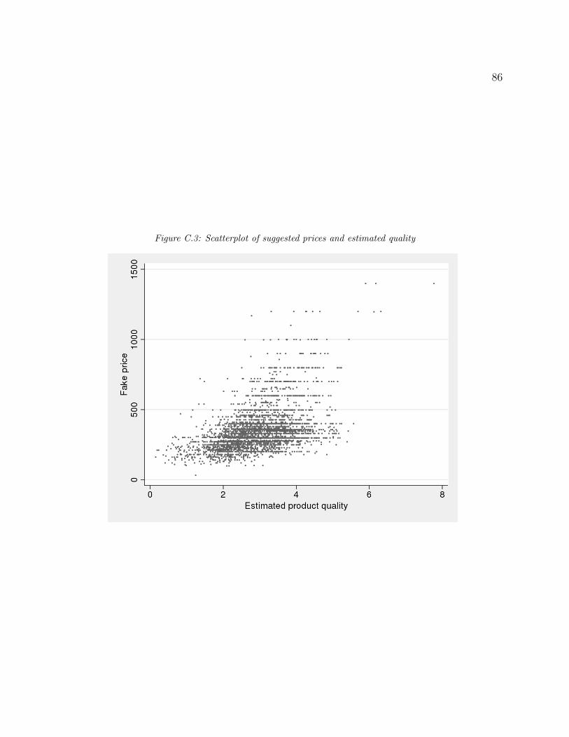
86
Figure C.3: Scatterplot of suggested prices and estimated quality

87
Table C.4: Shifting with store average discount percent
(1) (2)IV With shifter
pj -0.00746*** -0.00734***[8.63e-05] [8.55e-05]
suggested pj 0.000758*** -0.00546***[6.30e-05] [0.000264]
suggested pj × ave disc pct 0.00986***[0.000400]
age -0.000183*** -0.000189***[1.02e-05] [1.02e-05]
factory -0.287*** -0.293***[0.00843] [0.00841]
constant -6.328*** -6.375***[0.0541] [0.0541]
Observations 429,730 429,730R-squared 0.527 0.526
Standard errors in brackets*** p<0.01, ** p<0.05, * p<0.1

88
Figure C.4: Prices over time