Embed Size (px)
Citation preview

ECO 171
Nonlinear pricing
Second degree price discrimination

ECO 171
Self-selection
What if the seller cannot distinguish between
buyers?
perhaps they differ in income (unobservable)
Then the type of price discrimination just discussed
is impossible
High-income buyer will pretend to be a low-income
buyer
to avoid the high entry price
to pay the smaller total charge
Take a specific example
Ph = 16 – Qh
Pl = 12 – Ql
MC = 4

ECO 171
Second-degree price discrimination 2
First-degree price discrimination requires:
High Income: entry fee $72 and $4 per drink or entry plus
12 drinks for a total charge of $120
Low Income: entry fee $32 and $4 per drink or entry plus 8
drinks for total charge of $64
This will not work
high income types get no consumer surplus from the
package designed for them but get consumer surplus from
the other package
so they will pretend to be low income even if this limits the
number of drinks they can buy
Need to design a “menu” of offerings targeted at the
two types
ECO 171
Second-degree price discrimination 3
The seller has to compromise
Design a pricing scheme that makes buyers
reveal their true types
self-select the quantity/price package designed for
them
Essence of second-degree price
discrimination
It is “like” first-degree price discrimination
the seller knows that there are buyers of different types
but the seller is not able to identify the different types
A two-part tariff is ineffective
allows deception by buyers
Use quantity discounting

ECO 171
Simple example
p q
5 1
3 2
p q
4 1
1 2
Consumer 1
Consumer 2
• mc = 0
• If possible to separate:
• Sell 2 units to each.
• Charge consumer 1 a total of
$8 and consumer 2 a total of $5.
• This does not work if unable to
separate.
• Whatever alternative is offered to
consumer 2, the other type could
choose.
• Self-selection
• Instruments to discriminate:
handicap one of the alternatives.
• How: making it smaller!

ECO 171
Simple example - continued
p q
5 1
3 2
p q
4 1
1 2
Consumer 1
Consumer 2
Size of
package
Value to
consumer 1
Value to
consumer 2
1 5 4
2 8 5
• Looks like the self-selection problem of business and
tourists. Discrimination:
• Set price of package with one unit = 4
• Price of package with two units = 7
• Profits = $11
• Implementation:
1. Sell two packages
2. Offer a pair of two-part tariffs: F1=4, p1=3,
F2=0, p2=4.
3. Nonlinear price: unit 1 = $4, unit 2 = $3

ECO 171
Example 2 – discrimination not worthwhile
p q
4 1
2 2
p q
3 1
2 2
Consumer 1
Consumer 2
Size of
package
Value to
consumer 1
Value to
consumer 2
1 4 3
2 6 5
• Discrimination:
• Set price of package with one unit = 3
• Price of package with two units = 5
• Profits = $8
• Alternative 1: two units for both: $10
• Alternative 2: exclude consumer 2: $6

ECO 171
Example 2 – Exclude consumer 2
p q
5 1
3 2
p q
2 1
1 2
Consumer 1
Consumer 2
Size of
package
Value to
consumer 1
Value to
consumer 2
1 5 2
2 8 3
• Discrimination:
• Set price of package with one unit = 2
• Price of package with two units = 5
• Profits = $7
• Alternative 1: two units for both: $6
• Alternative 2: exclude consumer 2: $8

ECO 171
Examples – conclusions
Too discriminate, need to offer different alternatives.
Consumers must self-select.
This is done by “damaging” the alternative for low paying consumers: lower quantity
Then offer a price for small package and price for large package.
Cost: inefficient consumption of L type (deadweight loss)
Gain: Extract more CS from high type
When differences in willingness to pay are high, it pays to restrict quantity to L type.
Leave no CS to L type:
Charge the highest possible price
This way get more from the L type and lower the CS of high type.

ECO 171
Optimal exclusion of L type
q p1 p2 Gain from
including L type
(1)
Change in CS of
high type
(2)
Example 1
1 5 4
2 3 1
Example 2
1 4 3
2 2 2
Example 3
1 5 2
2 3 1
Net:
(1)-(2)

ECO 171
With continuous demand functions
Ph = 4 – Qh
PL = 2 – QL
MC = 0
1. Sell 2 units to type L
2. Set price for this two units
equal to total surplus = area
under demand = 2*2/2=2
3. What can offer to H type?
- Quantity = 4
- Charge: ?
4. Profits = 2 NL + 4 Nh
5. e.g. if NL = Nh =N, profits = 6N

ECO 171
Any better deal?
Ph = 4 – Qh
PL = 2 – QL
MC = 0
1. Sell 1 unit to type L
2. Set price for this unit equal to
total surplus = area under
demand = (2+1)/2 x 1 = 3/2
3. What can offer to H type?
- Quantity = 4
- CSh under L-plan = 2
- Maximum charge: 8-2=6
4. Profits = 3/2 NL + 6 Nh
5. e.g. NL = Nh = N, profit = 7 ½ N
ECO 171
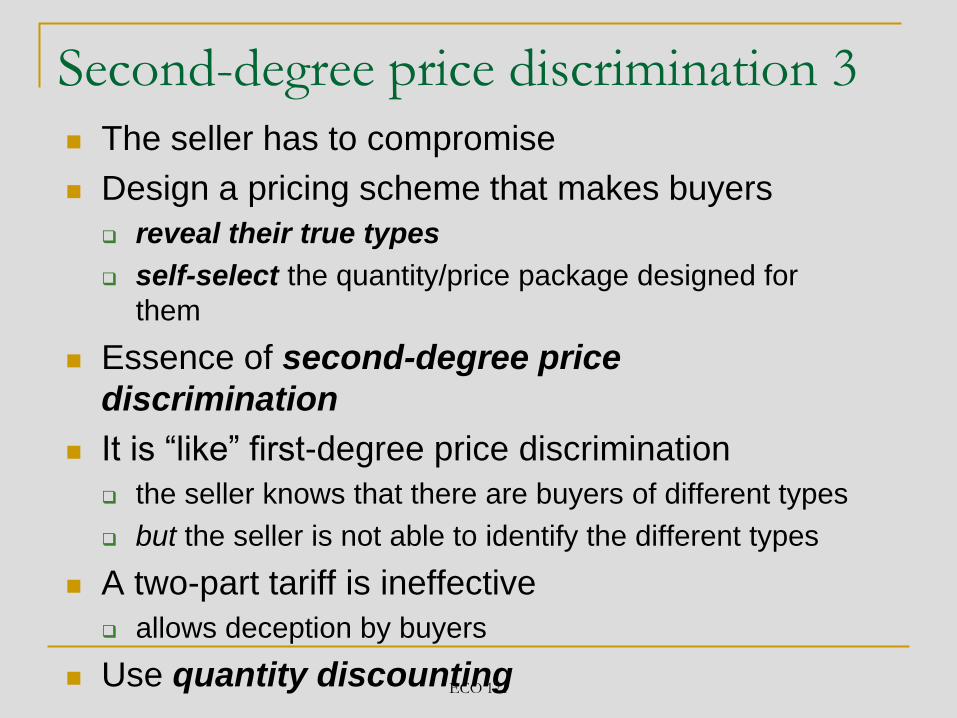
Optimal quantity
Effect of a small decrease in qL
-Loss from excluding L type: NL x qL x pL
- CSh = Nh x qL x (ph – pL )
- Net gain qL [ Nh x (ph – pL ) - NL x pL ]
If Nh=NL this is positive if ph-pL>pL.
Optimal quantity qL: cut quantity until Nh x (ph – pL ) = NL x pL
Note: if marginal cost is positive, until Nh x (ph – pL ) = NL x (pL – mc )
qL

ECO 171
Optimal quantity (continued)
In previous example, assuming Nh = NL
ph = 4-q, pL= 2-q
Condition is: (4-q – (2-q)) = 2-q q=0!
Best is to exclude completely type L.
Suppose NL = 2 x Nh
2 = 2 x (2-q)
q=1
Optimal quantity increases as NL / Nh increases
Intuition: losses from excluding L are proportional to NL and gain from more surplus extraction from h are proportional to Nh .
ECO 171
Optimal packages
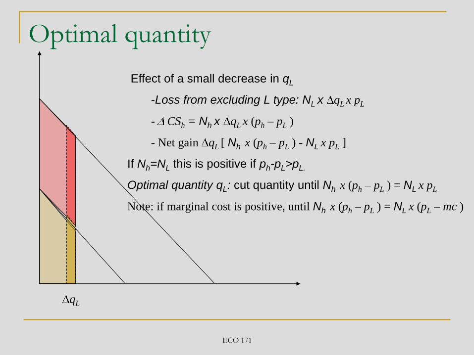
In previous example with NL = 2 Nh
qL = 1
Charge L: $ 1.5 (their total surplus)
qh = 4 (always quantity is efficient for h type)
Charge h: Total surplus minus utility under L plan
= 8-2 = 6
Total profits: 1.5 x NL + 6 x Nh

ECO 171
Set qL so that Nh x (ph-pL) = NL x (pL- mc)
Charge L-type their entire surplus (area under
demand curve up to qL ) =
Set qh at the efficient level: p(qh) = mc
Charge H-type their entire surplus minus the utility
they get under L-plan =
Optimal packages – general case
Lq
L dxxP0
h Lq q
Lhh dxxPxPdxxP0 0

ECO 171
Optimal packages – general principles
Characteristics of second-degree price discrimination extract all consumer surplus from the lowest-demand group
leave some consumer surplus for other groups the self-selection (also called incentive-compatibility) constraint.
offer less than the socially efficient quantity to all groups other than the highest-demand group
offer quantity-discounting
Second-degree price discrimination converts consumer surplus into profit less effectively than first-degree
Some consumer surplus is left “on the table” in order to induce high-demand groups to buy large quantities.
Fundamental tradeoff – restricting output to lower types to increase surplus extracted from higher types.
The higher the cost of this distortion or lower the added surplus extracted, the higher qL will be.
It may be optimal to exclude L types.

ECO 171
Generalization to many consumer types
F1
F2
• Total price schedule is concave
• Derivative interpreted as marginal price, i.e price
for the last unit.
• Can approximate by offering these two plans:
T1 (q) = F1 + p1
q
T2 (q) = F2 + p2
q
Total
quantity
Total
price Optimal price
schedule

ECO 171
Non-linear pricing and welfare
Non-linear price
discrimination raises profit
Does it increase social
welfare?
suppose that inverse
demand of consumer group
i is P = Pi(Q)
marginal cost is constant at
MC – c
suppose quantity offered to
consumer group i is Qi
total surplus – consumer
surplus plus profit –is the
area between the inverse
demand and marginal cost
up to quantity Qi
Price
Quantity
Demand
c MC
Qi Qi(c)
Total
Surplus

ECO 171
Non-linear pricing and welfare 2
Pricing policy affects
distribution of surplus
output of the firm
First is welfare neutral
Second affects welfare
Does it increase social
welfare?
Price discrimination
increases social welfare of
group i if it increases
quantity supplied to group i
Price
Quantity
Demand
c MC
Qi Qi(c)
Total
Surplus
Q’i
ECO 171
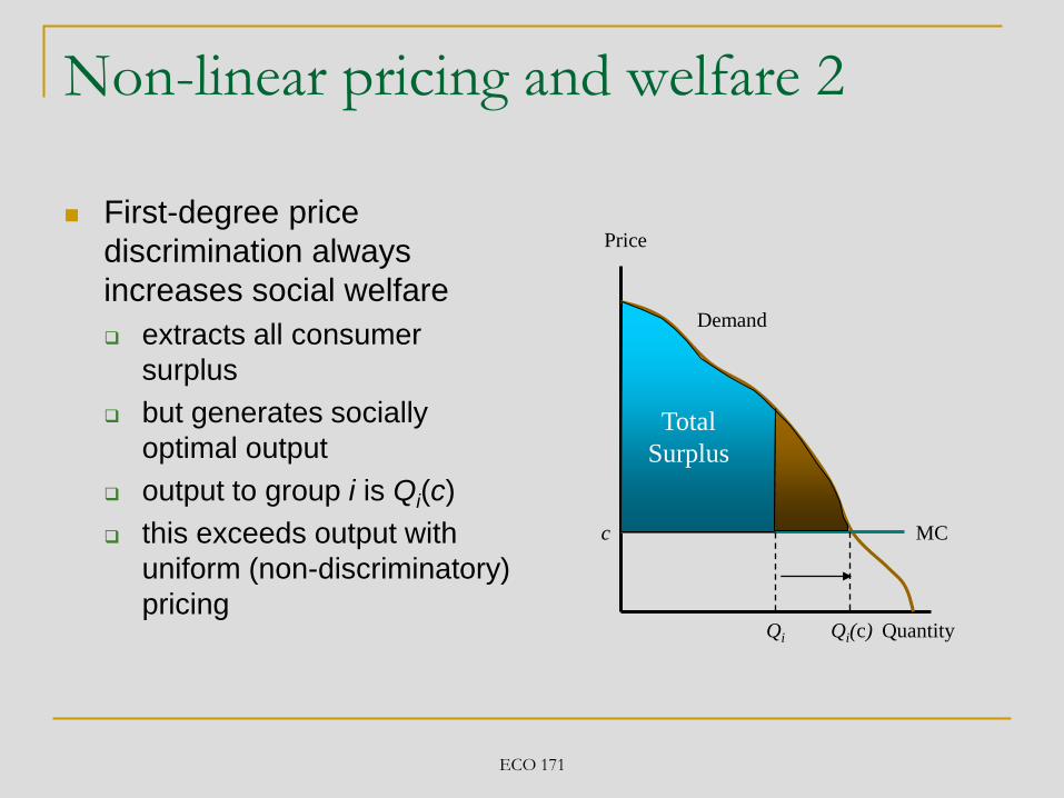
Non-linear pricing and welfare 2
First-degree price
discrimination always
increases social welfare
extracts all consumer
surplus
but generates socially
optimal output
output to group i is Qi(c)
this exceeds output with
uniform (non-discriminatory)
pricing
Price
Quantity
Demand
c MC
Qi Qi(c)
Total
Surplus
ECO 171
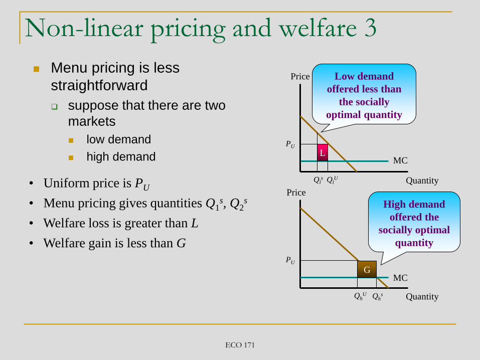
Non-linear pricing and welfare 3
Menu pricing is less
straightforward
suppose that there are two
markets
low demand
high demand
Price
Quantity
Price
Quantity
MC
MC
• Uniform price is PU
• Menu pricing gives quantities Q1s, Q2
s
PU
PU
QlU
QhU
• Welfare loss is greater than L
• Welfare gain is less than G
Qls
Qhs
L
G
High demand
offered the
socially optimal
quantity
Low demand
offered less than
the socially
optimal quantity

ECO 171
Non-linear pricing and welfare 4
Price
Quantity
Price
Quantity
MC
MC
PU
PU
QlU
QhU
Qls
Qhs
L
G
= (PU – MC)ΔQ1 + (PU – MC)ΔQ2
= (PU – MC)(ΔQ1 + ΔQ2)
ΔW < G – L
A necessary condition for second-
degree price discrimination to
increase social welfare is that it
increases total output
It follows that
“Like” third-degree price
discrimination
But second-degree price
discrimination is more likely to
increase output

ECO 171
The incentive compatibility constraint
Any offer made to high demand consumers must
offer them as much consumer surplus as they
would get from an offer designed for low-
demand consumers.
This is a common phenomenon
performance bonuses must encourage effort
insurance policies need large deductibles to deter cheating
piece rates in factories have to be accompanied by strict
quality inspection
encouragement to buy in bulk must offer a price discount