Embed Size (px)
Citation preview

The Pennsylvania State University
The Graduate School
The Mary Jean and Frank P. Smeal College of Business
ESSAYS ON MARKET FRICTIONS IN THE
REAL ESTATE MARKET
A Dissertation in
Business Administration
by
Sun Young Park
Copyright 2012 Sun Young Park
Submitted in Partial Fulfillment
of the Requirements
for the Degree of
Doctor of Philosophy
August 2012

The dissertation of Sun Young Park was reviewed and approved* by the following:
Brent W. Ambrose
Smeal Professor of Real Estate Head of Smeal College Ph.D. Program
Dissertation Adviser
Chair of Committee
Austin J. Jaffe
Chair, Department of Risk Management
Philip H. Sieg Professor of Business Administration
N. Edward Coulson
King Faculty Fellow and Professor of Real Estate Economics
Jiro Yoshida
Assistant Professor of Business
Jingzhi Huang
Associate Professor of Finance and McKinley Professor of Business
*Signatures are on file in the Graduate School

ABSTRACT
The real estate market is generally considered a less complete asset market than other
financial asset markets in that real estate assets carry higher holding costs than other
financial assets do. Thus, the real estate market is a good laboratory in which to explore
the topic of market frictions. If a market were perfectly liquid such that no market
frictions exist, the efficient market hypothesis would hold. However, as the 2007–2008
financial crisis has shown, market frictions arise for various reasons: asymmetric
information, transaction costs, and financial constraints. The law of one price does not
hold under the existence of market frictions. Thus, market frictions have important
implications for the limits of arbitrage. It is important to understand the impact of market
frictions and the ways in which they call into question the principles of classical
economics.
In order to examine market frictions, I focus on two categories: liquidity and
segmentation. My dissertation offers a consideration of market frictions as follows:
Chapter 1 presents an overview of market frictions in the real estate market together with
an outline of the dissertation; Chapter 2 examines the spill-over impact of liquidity shocks
in the commercial real estate market; Chapter 3 considers market segmentation by
investor type in the commercial real estate market; Chapter 4 focuses on the liquidity
spiral between market liquidity and loss aversion; and Chapter 5 presents concluding
remarks.

iv
TABLE OF CONTENTS
LIST OF FIGURES ............................................................................................................................................ vi
LIST OF TABLES ............................................................................................................................................. vii
ACKNOWLEDGEMENTS ............................................................................................................................ viii
Chapter 1. Overview of Market Frictions in the Real Estate Market ....................................................... 1
Chapter 2. The Spill-Over Impact of Liquidity Shocks in the Commercial Real Estate Market........ 6
Literature Review ........................................................................................................................................ 8
Liquidity Measures ................................................................................................................................... 13
Stock Market ............................................................................................................................ 13
CDS Market .............................................................................................................................. 14
Bond Market ............................................................................................................................. 15
Underlying Assets (Private Market) ................................................................................... 16
Study Design .............................................................................................................................................. 18
Descriptive Statistics ................................................................................................................................ 19
Vector Auto Regression ........................................................................................................................... 21
CDS Market .............................................................................................................................. 21
Stock and Bond Markets ........................................................................................................ 23
Underlying-Asset Market ...................................................................................................... 24
Granger Causality Test ............................................................................................................................. 25
Impulse Response Function .................................................................................................................... 26
Variance Decomposition ......................................................................................................................... 27
Robustness Check ..................................................................................................................................... 29
Summary of Findings ............................................................................................................................... 31
Chapter 3. Does the Law of One Price Hold in Heterogeneous Asset Markets? ................................. 52
Literature Review ...................................................................................................................................... 56
Segmentation Type ................................................................................................................................... 60
Hypotheses .................................................................................................................................................. 61
Data............................................................................................................................................................... 62
Methodology .............................................................................................................................................. 63

v
Summary Statistics .................................................................................................................................... 69
Empirical Results ...................................................................................................................................... 70
Type I Segmentation ............................................................................................................... 70
Type II and Type III segmentation ...................................................................................... 75
Summary of Findings ............................................................................................................................... 77
Chapter 4. Loss Aversion and Market Liquidity in the Commercial Real Estate Market ............... 104
Literature Review ................................................................................................................................... 107
Methodology ........................................................................................................................................... 110
Loss Aversion and Liquidity Measure ............................................................................................... 112
Descriptive Statistics ............................................................................................................................. 115
Empirical Results ................................................................................................................................... 117
Loss Aversion and Private Market Liquidity ................................................................. 117
Loss Aversion and Stock Market Liquidity ................................................................... 120
Loss Aversion and Financial Constraints ....................................................................... 124
Summary of Findings ............................................................................................................................ 126
Chapter 5. Concluding Remarks .................................................................................................................. 134
Bibliography ..................................................................................................................................................... 137

vi
LIST OF FIGURES
Figure 2-1: Monthly Time-Series of the dSPOfferClose ............................................................. 33
Figure 2-2: Response of REIT to Generalized One SD Shock in BOND ..................................... 34
Figure 2-3: Response of BOND to Generalized One SD Shock in REIT ..................................... 35
Figure 2-4: Response of CDS to Generalized One SD Shock in BOND ...................................... 35
Figure 2-5: Response of BOND to Generalized One SD shock in the Private Market ............. 36
Figure 2-6: Response of Private Market to Generalized One SD Shock in BOND ................... 36
Figure 2-7: Forecast Variance Decomposition for CDS ................................................................... 37
Figure 2-8: Forecast Variance Decomposition for BOND ............................................................... 37
Figure 2-9: Forecast Variance Decomposition for REIT ................................................................. 38
Figure 2-10: Forecast Variance Decomposition for PRIVATE Market ........................................ 38
Figure 3-1: Summary of Matching Results.......................................................................................... 80
Figure 3-2: Hedonic Regression with Two Investor Types ............................................................. 81
Figure 3-3: Three Types of Market Segmentation ............................................................................. 82
Figure 3-4: The Testing Procedure ........................................................................................................ 83
Figure 3-5: Box Plot for the log (size_sf) ............................................................................................ 84
Figure 3-6: Box Plot for Building Age ................................................................................................. 86

vii
LIST OF TABLES
Table 2-1: Descriptive Statistics ............................................................................................................ 39
Table 2-2: Correlations ............................................................................................................................. 40
Table 2-3: VAR using the OfferClosedSP with 2-month lag .......................................................... 41
Table 2-4: Granger Causality .................................................................................................................. 42
Table 2-5: Decomposition of Variance for CDS
t .......................................................................... 43
Table 2-6: Decomposition of Variance for BOND
t ....................................................................... 44
Table 2-7: Decomposition of Variance for REIT
t ......................................................................... 45
Table 2-8: Decomposition of Variance for tdSPOfferClose ..................................................... 46
Table 2-9: VAR using the CapRateSP with a 2-month lag .............................................................. 47
Table 2-10: VAR using the BidAskSP with a 2-month lag ............................................................. 48
Table 2-11: VAR using the 5YR Treasury-Bill with a 2-month lag .............................................. 49
Table 2-12: REITs with CDS contracts ................................................................................................ 50
Table 2-13: REITs with Traded Bonds ................................................................................................. 51
Table 3-1: Descriptive Statistics I .......................................................................................................... 87
Table 3-2: Descriptive Statistics II ........................................................................................................ 88
Table 3-3: Description and Definition of Investor Type .................................................................. 90
Table 3-4: Average Effect of Treatment on the Treated (ATT) ...................................................... 91
Table 3-5: Mean Price Difference of Matched Samples: Type I .................................................... 92
Table 3-6: The Difference in the Marginal Factor Price: Type II .................................................. 94
Table 3-7: The Discontinuity of Price Functions: Type III .............................................................. 98
Table 4-1: Descriptive Statistics ......................................................................................................... 128
Table 4-2: Cox Hazard Regression with Private Market Liquidity ............................................. 129
Table 4-3: Cox Hazard Regression with Bid-Ask Spread ............................................................. 130
Table 4-4: Cox Hazard Regression with Prospective Gain and Bid-Ask Spread..................... 131
Table 4-5: Cox Hazard Regression with Amihud Liquidity Measure ........................................ 132
Table 4-6: Cox Hazard Regression with Financial Constraints ................................................... 133

viii
ACKNOWLEDGEMENTS
First and foremost, I would like to express my deepest gratitude to my advisor, Dr.
Brent Ambrose. Without his encouragement and support, this dissertation would never
have been possible. In my journey, Dr. Ambrose has been my greatest inspiration.
I would like to thank all my committee members: Dr. Austin Jaffe, Dr. Edward Coulson,
Dr. Jiro Yoshida, and Dr. Jingzhi Huang. I would like to express special thanks to Dr.
Jaffe, who shared his insights and guided me in establishing a new research agenda. I
would also like to express my sincere gratitude to Dr. Yoshida for his patience and
steadfast encouragement as I worked on Chapter 3 of this dissertation.
I must not forget to mention Seo Jin Cheong, who encouraged me to study abroad
and pursue my Ph.D. And, my dearest friend, Ji Sook Park, gave me the strength to go on
this journey. Likewise, I cannot thank Seok Jae Yoon and Seung Mi Baik enough: they
brought me comfort and gave me courage throughout my whole journey.
Last but not the least, this dissertation would not have been possible without the great
love and care I received from my parents Yu Gyeon Park, Gyeong Suk Lee, and from my
brother, Seong Woo Park.

1
Chapter 1
Overview of Market Frictions in the Real Estate Market
The efficient market hypothesis holds that the market is complete and that transactions
occur such that assets realize a fair price. However, in practice, transaction costs and
asymmetric information make asset markets less complete than other financial asset
markets. Thus, market frictions arise. The law of one price does not hold under the
existence of market frictions. Thus, market frictions have important implications for the
limits of arbitrage. Accordingly, it is important to understand the impact of market frictions
and the ways in which they call into question the principles of classical economics.
According to the literature, two phenomena are related to the market frictions that lead
to incomplete asset markets: liquidity and segmentation.1 It is necessary to consider
liquidity and segmentation if we are to find answers to fundamental questions such as these:
To what extent is the market incomplete? How do asset markets function differently under
market frictions? What implications do market frictions have for the principles of classical
economics?
Related to these questions, segmentation prevents arbitrageurs from providing enough
liquidity to the market at the most necessary time. Thus, segmentation and liquidity are
closely related. However, a number of subtle differences should be accounted for:
Segmentation prevents investors from sharing investment risks across different asset
1 See Cochrane (2011) for a discussion of three kinds of market frictions: segmented markets, intermediated
markets, and liquidity.

2
markets. On the other hand, liquidity is a feature of assets and generally refers to the
relative ease with which trades can be made without resulting in a significant change in
price. The less liquid the market, the harder it is to complete a market transaction. In
extreme cases, the market completely shuts down such that it ceases to exist. Therefore,
segmentation is about limited risk-bearing ability, whereas liquidity is about trading.2
Given the scholarly consensus on the importance of these topics, we should ask what
the real estate market is particularly concerned with. The heterogeneity of individual
properties and locations creates market frictions among investors, and as a result the real
estate market may be more segmented than the common security market. It is more
important, therefore, to consider market frictions closely in the real estate market than it is
to do so in other financial markets. Aligned with this general idea, the objective of my
research is to investigate how market frictions—liquidity and segmentation—relate to and
undermine the principles of classical economics.
The dissertation is structured in order to provide specific descriptions of concepts
chapter by chapter and yet to connect those concepts throughout. Chapter 1 presents an
overview of market frictions in the real estate market together with an outline of the
dissertation; Chapter 2 examines the spill-over impact of liquidity shocks in the commercial
real estate market; Chapter 3 considers market segmentation by investor type in the
commercial real estate market; Chapter 4 focuses on the liquidity spiral between market
liquidity and loss aversion; and Chapter 5 presents concluding remarks.
Liquidity is closely related to price discovery in asset transactions. In particular, given
the fact that the commercial real estate market is characterized as relatively illiquid due to
2 See Cochrane (2011).

3
both its underlying heterogeneous characteristics, determining the impact of liquidity on the
real estate market requires a unique analytical approach.
Chapter 2 examines the liquidity spill-over impact across four real estate markets: the
stock (Real Estate Investment Trust (REIT) equity) market, the derivative (Credit Default
Swap (CDS)) market, the corporate-bond market, and the private real estate (property sale–
based) market. Considerable anecdotal evidence suggests that the effects of liquidity shocks
spread quickly throughout the financial sector. However, few studies have focused on the
dynamics of liquidity across real estate markets. Given the fundamental link between the
underlying assets of the private and public real estate markets, liquidity shocks are
especially likely to spill over across these particular markets—a point that has important
implications for investment allocation and portfolio management. Employing a Vector Auto
Regression (VAR) methodology, I find that bond-market liquidity shocks negatively impact
CDS market-liquidity with a 2-month lag. Furthermore, stock-market liquidity shocks
Granger Cause bond-market liquidity with a 2-month lag. Variance decomposition analysis
also supports the finding that the main cause of fluctuations in bond-market liquidity is
liquidity shocks in the stock market. Shocks to underlying-asset liquidity also have a
moderate impact on fluctuations in bond-market liquidity. Underlying asset liquidity
(private-market liquidity) Granger Causes bond-market liquidity, a relation that also holds
vice versa. However, the spill-over impact of underlying asset liquidity (private-market
liquidity) on the public real-estate market varies in accordance with different measures.
On the other hand, the commercial real estate market is constrained by high holding
costs, which prevents arbitrageurs from eliminating mispricing. Thus, the limits of arbitrage
are also called into question in the real estate market. Therefore, if the commercial real

4
estate market is not free from the limits of arbitrage due to high holding costs, whether
market segmentation exists is an empirical question that requires an answer.
Chapter 3 empirically examines the possibility and implications of market
segmentation. The existence of market segmentation violates the law of one price; therefore,
it is important to understand how and the extent to which the market is segmented. In
particular, I am interested in investigating market segmentation by investor type: This kind
of segmentation differs from standard segmentation in that the former relies on
heterogeneous locations and property types and the latter relies on investor type. Several
phenomena—non-fundamental risks, holding costs, leverage constraints, and equity
constraints—account for why arbitrageurs cannot eliminate mispricing, and as a result
pricing may differ by investor type.3 I find empirical evidence against the law of one price
for an important class of heterogeneous assets, i.e., commercial real estate. I consider three
types of possible market segmentation. First, matching estimation identifies cases in which
transaction prices for comparable assets, on average, differ by investor type. Second, even if
average prices do not differ for comparable assets, marginal factor prices differ among
some investor types. Third, when investors differ in terms of the domain each focuses on, I
find cases of discontinuity in the factor price functions. Using propensity-score matching
and regression analysis for 21 combinations of investor types in each property-type market,
I find market segmentation as follows: 8 pairs for office, 13 for retail, 11 for industry, and 7
for the multi-family market.
Chapter 4 offers a consideration of loss aversion and market liquidity in the real estate
market. Conventional wisdom in the financial literature asserts that the more risk-averse the
3 See Gromb and Vayanos (2010) for a survey of the limits of arbitrage

5
investors, the less liquid the market, and that loss aversion is the most commonly observed
risk-averse behavior in the commercial real estate market. Loss aversion refers to investors
who are more sensitive to prospective losses than to prospective gains. The fact that
commercial real estate investors appear to be loss averse suggests the following questions:
Does the commercial real estate market rationally anticipate investor loss aversion? Does
market liquidity amplify investor loss aversion? Does a financial crisis change the pattern of
loss aversion? The answers to these questions have strategically important implications for
real estate investors, as an interaction between market liquidity and loss aversion may
increase actual investment risk.
I predict that both private and public market liquidity amplify seller loss aversion such
that declines in market liquidity reduce the impact of potential gains (or losses) on the sale
probability of properties. I empirically test this hypothesis by examining the probability of
property transactions for real estate investment trusts (REITs). The empirical results
demonstrate that a financial crisis matters to the relation between liquidity and loss aversion.
That is, when a financial crisis is not controlled for, low levels of stock market and private
market liquidity reduce the impact of prospective gains (or losses) on the sale probability of
property in a market downturn, thereby heightening sellers’ loss-aversion behavior.
However, when a financial crisis is controlled for, the effect of prospective gains (or losses)
does not hold whereas the impact of stock market and private market liquidity still holds. I
interpret the sellers’ reluctance during a crisis period to take a loss in a less liquid market as
overriding their interest in realizing a gain. Thus, I conclude that the pattern of loss aversion
during a crisis period may differ from the pattern during a period.

6
Chapter 2
The Spill-Over Impact of Liquidity Shocks in
the Commercial Real Estate Market4
During the recent financial crisis, the notion of liquidity and the factors that create it
garnered considerable academic attention. In general, a liquid market is one where an asset
can be sold at a fair price—one that reflects the asset’s fundamental value regardless of
overall market conditions. Numerous events including the Long Term Capital Management
(LTCM) crisis, the collapse of Bear Stearns, and the subprime mortgage crisis provide
considerable anecdotal evidence that once a liquidity shock has occurred, its effects spread
quickly throughout the financial sector.
By definition, illiquidity arises from a wedge between the fundamental asset value and
market price.5 I posit that fundamental changes in asset markets do not occur in the short
term, and thus liquidity shocks are related to the short-term asset price fluctuation beyond
the market fundamentals. Accordingly, I define liquidity shocks as short-term decreases in
liquidity in one market that generate a chain reaction in other markets.
Liquidity is associated with several interesting issues in the real estate market. First,
4 This chapter is based on a paper co-authored with Brent Ambrose.
5 Cochrane (2011) argues that liquidity can refer to instances in which an individual security is bought and sold and
that illiquidity can be systemic. In other words, assets can face a higher discount rate when the market as a whole is
illiquid regardless of the fundamental asset value.

7
real estate has a distinctive feature that may be responsible for amplifying the impact of any
given liquidity shock; that is, the private real-estate (property sale–based) market and the
public real-estate market share an underlying asset connection. As a result, it is possible to
use the liquidity of the private market as a basis for discerning the impact of a liquidity
shock across different markets. That is, by isolating the fundamental asset variation and
liquidity in the private market, I answer a key research question pertaining to how
fundamental asset liquidity affects other stock, bond, and derivative markets.
Second, by identifying the liquidity impact of the private market on these other
markets, I obtain additional insights into the relationship between the private and public
real-estate markets. Though the risk and adjusted-return relationship between the private
and public real-estate markets is well documented, few studies have concentrated on the
dynamics of liquidity between the two markets.6
Thus, my study has important
implications for portfolio management and investment allocations given that any given
liquidity shock may have an interdependent effect on the private and public markets.
More specifically, I propose to answer the following questions: Do liquidity shocks
spill over across private and public real-estate markets? Is one of the markets more likely to
lead or follow a liquidity shock than the other? Does private market liquidity derive from
public market liquidity or vice versa? Although numerous studies in the finance literature
focus on the liquidity of derivative markets such as the Credit Default Swap (CDS) market,
I contribute to this literature by studying how liquidity shocks evolve across the stock, bond,
derivative, and private real-estate markets.
6 Pagliari, Scherer, and Monopoli (2005) investigate whether public and private real estate return series show
statistical differences. The authors show that the average difference between two return series is very small and
conclude that public- and private-market vehicles are synchronous in the long term.

8
This chapter is organized as follows: The first section presents a review of the
literature relevant to market liquidity and its spill-over effects on respective markets. Next, I
summarize the research methodology and offer a description of the data collected. This
account is followed by a description of the liquidity measures used in the test models. In the
subsequent sections, the main results obtained using the Vector Auto Regression (VAR)
model are described, as are the robustness check tests. The concluding section offers a
summary of the research and its implications.
Literature Review
In a perfectly liquid market, no market friction exists; that is, there is no wedge
between an asset’s transaction price and its fundamental value.7 And, under such
conditions, the efficient market hypothesis holds. However, realistically, market
transactions are susceptible to various market frictions driven by asymmetric information,
capital constraints, and transaction costs. Therefore, it is important to understand the
connection between underlying asset liquidity and its impact on the advanced securities
derived from those underlying assets.
Brunnermeier and Pedersen (2009) present a theoretical framework for analyzing
liquidity spirals in the security market. In their model, a shock to security prices (or
volatility) during a market downturn restricts the ability of market makers to obtain
necessary funding. Furthermore, this restriction causes a substantial drop in market liquidity.
Taken together, funding liquidity and market liquidity reinforce each other to create
liquidity commonality.
7 See Brunnermeier and Pedersen (2009).

9
A significant number of papers have investigated liquidity commonality within and
across multiple markets. For example, Acharya and Pederson (2005) provide a framework
for considering how the risk arising from commonality in liquidity is priced in the stock
return and show that the required return of a security increases in the covariance between its
illiquidity and market illiquidity. In addition, recent studies have shown that liquidity can
spill over from one market to another. For example, Chorida, Sarkar, and Subrahmanyam
(2005) investigate cross-market liquidity dynamics showing the co-movement of liquidity
and volatility between the stock and Treasury-bond markets.
In general, the heterogeneous nature of real-estate assets leads to highly variable
liquidity in private asset markets. For example, Fisher, Gatzlaff, Geltner, and Haurin (2003)
focus on the impact of variable liquidity on the transaction-based index, showing that the
liquidity factor might explain why the private-market index lags behind that of the public-
market. Furthermore, Benveniste, Capozza, and Seguin (2001) suggest that liquidity in the
underlying property market also plays a significant role in determining price changes and
liquidity in the public REIT market.8
The interaction between market liquidity and capital constraints is a fairly new
research topic. For example, Ling, Naranjo, and Scheick (2011) conclude that credit
availability is a key factor in determining price movements in both the private and the
public REIT markets, and they find a feedback effect between market liquidity and credit
availability. Bond and Chang (2011) investigate cross-asset liquidity between equity
8 Aligned with this research agenda, Clayton, MacKinnon, and Peng (2008) show that real-estate investors place a
greater value on the liquidity of REITs when private market liquidity is low, expressing their priorities by shifting
their holdings to the public market as the private real-estate market becomes increasingly illiquid. Brounen,
Eichholtz, and Ling (2009) document the impact of the liquidity factor on the returns of the public real-estate
market using global REIT stock and conclude that market capitalization, nonretail-share ownership, and dividend
yields serve as drivers of liquidity across countries.

10
markets and REITs and between REITs and private real estate markets. They find that
REITs exhibit lower levels of liquidity as compared to a set of control firms matched in
terms of size and book to market ratios. Additionally, using a proxy for private market
liquidity, i.e., the volatility of asset returns during the time to sale, the authors also find
significant directional causality for most liquidity proxies.
The present study departs from previous research in several important ways. First, in
addition to the stock market, I include the CDS and bond markets and use broader asset
classes than the previous literature does. Second, I focus on the spill-over impact across a
variety of asset classes whereas Bond and Chang (2011) focus on commonality and intraday
liquidity movements. Third, I introduce a unique private-market liquidity measure,
dSPOfferClose , which is equal to the spread between the offered and the closed cap rates.
The present study is also related to the burgeoning literature on contagion. Generally
speaking, contagion is defined as a shock in one country that generates price movements in
other countries. Accordingly, contagion provides a potential alternative way to explain the
spill-over phenomenon of market crashes.
Four branches of the literature focus on explaining contagion. One branch emphasizes
the “flight-to-quality” effect according to which investors holding multiple assets intend to
switch their portfolios from “poor-quality” to “high-quality” markets in terms of market
performance. For example, Hartmann, Straetmans, and de Vries (2004) investigate the
contagion phenomenon of market returns as it applies to the stock and bond markets. They
demonstrate that a crash in the stock market is accompanied by a boom in the government
bond market and conclude that this is a result of the flight-to-quality effect. I focus on the
flight-to-quality effect driven by the liquidity conditions of each market and show that

11
investors’ tendency to seek highly liquid markets determines the outcome; that is, a
liquidity crash in one market is accompanied by a liquidity boom in another. I also
demonstrate that the liquidity channel in each market is a key element in determining the
extent to which shocks spread across multiple asset markets. For example, investors prefer
selling assets in a more liquid market over doing so in a less liquid market, as illiquidity
lowers liquidation values. The role of the liquidity channel in transmitting shocks across
multiple asset markets is well demonstrated in the literature.9
A second branch emphasizes the information effect, which is related to the
vulnerability of imperfect financial markets. In regard to the correlated information channel,
price changes in one market are perceived as having implications for the values of assets in
other markets such that price changes in the former actually give rise to price changes in the
latter.10
A third branch emphasizes the “portfolio rebalancing” effect, which is based on the
rational expectation model. According to Kodres and Pritsker (2002), investors transmit
idiosyncratic shocks from one market to others by adjusting their portfolios’ exposure to
shared macroeconomic risks. In turn, shared macroeconomic risks compose the liquidation
value of assets in each market and determine the pattern and severity of financial contagion
and the degree of the information asymmetry in each market.
A fourth branch emphasizes the role of the “wealth effect” in causing self-fulfilling
crises. Goldstein and Pauzner (2004) posit that if two countries have independent
9 Calvo and Mendoza (2000) and Yuan (2002) document that when some investors choose to liquidate some of
their assets in a number of markets due to a call for additional collateral, sales in these multiple markets generate
the spill-over of market crashes.
10 King and Wadhwani (1990).

12
fundamentals but share the same group of investors, investors will withdraw their
investments fearing other investors’ reactions. A crisis in country A reduces investors’
wealth in that country, and this makes them more averse to the strategic risks associated
with the unknown behavior of investors in country B. Thus, the investors in country A
become more motivated than in the pre-crisis period to withdraw their investments from
both countries.
However, the majority of the literature on contagion focuses on analyzing price
movements across different countries and stops short of performing a cross-asset market
analysis. I distinguish my research from the previous literature in that I investigate the spill-
over impact of liquidity shocks across multiple real estate markets.
From the perspective of methodology, I build on Jacoby, Jiang, and Theocharides
(2010), who investigate cross-market liquidity shocks as they affect general firms in the
CDS, corporate bond, and equity markets. They find evidence of a 3-month time lag for
liquidity-shock spill-over from the CDS to both the bond and equity markets, but no clear
liquidity shock spill-over between the equity and bond markets.
I advance the work of the previous literature in several ways. First, by focusing on the
real-estate markets, I am able to incorporate the liquidity of underlying assets in the private
market. The commercial real-estate market is considered relatively illiquid due to
heterogeneous locations and property types. Accordingly, liquidity shocks and their patterns
in the real-estate market require a specific analysis―one that focuses only on the real estate
markets.
Second, by including private-market liquidity in this analysis, I provide another
perspective on the relationship between the private and public real-estate markets at least in

13
terms of liquidity-shock spill-over. The existence and direction of the spill-over of liquidity
shocks between the private and public real-estate markets is a long-standing open question.
To my knowledge, few papers directly test the liquidity-shock spill-over across the private
and public real-estate markets.
Liquidity Measures
In order to study the effects of liquidity shocks across multiple markets, I take into
account the unique feature of commercial real estate: observable trading prices on different
financial claims on the underlying asset in multiple markets. Thus, I collected information
on the market prices of financial contracts that are based on commercial real estate from
multiple data sources.
Stock Market
To test the effects of liquidity shocks in the stock market, I employ two liquidity
measures. First, I modify Amihud’s (2002) illiquidity measure (AIL) as a proxy for stock
market liquidity. AIL is the monthly average ratio of each REIT’s daily absolute return to its
daily dollar trading volume:
didi
miD
d
mimi VOLRDAIL ,,
,
1=
,, /1/= (1)
where diR , is the daily return for REIT i, diVOL , is the daily REIT i dollar volume, and
miD , is the number of days for which data are available for REIT i in month m. I collected
daily stock returns for the REITs from the Center for Research in Security Prices (CRSP). I
then created an aggregate stock market liquidity measure by taking the equally weighted

14
average of the individual REIT monthly Amihud measures (multiplied by 610 ):
6
,1=
10*1/= mi
mN
im
REIT
m AILNLIQ (2)
where mN represents the number of REITs in month m.
My second stock market liquidity measure is based on the common share price bid–ask
spread. I calculated the average of the monthly quoted spread ( miBidAskSP, ) for each REIT i
based on the daily ask price ( diAskP , ) and bid price ( di
BidP , ) from the CRSP daily database:
diBid
diAsk
miD
dmimi PPDBidAskSP ,,
,
1=,, 1/= (3)
I then created the second stock market liquidity measure by taking the equally
weighted average of the individual REIT monthly bid–ask spreads:
(4)
where again mN represents the number of REITs in month m.
CDS Market
In order to measure CDS market liquidity, I use the magnitude of price movement, a
relatively new measure for capturing transitory price movements.11
According to Kyle
(1985), market liquidity comprises three transactional characteristics: the cost of liquidating
a position over a short period of time (tightness), the ability to buy or sell large numbers of
shares with minimal price impact (depth), and the propensity of prices to recover quickly
11
See Bao, J., J. Pan and J. Wang (2011).

15
from a random uninformative shock to the market (resiliency). Bao, Pan, and Wang’s (2011)
measure is aligned with the depth of liquidity. Using their method, I constructed the
following measure for capturing negative covariances in CDS spread changes:
),(= 1,,, didi
cds
di SpreadSpreadcov (5)
where 1,,, = dididi SpreadSpreadSpread and dididi SpreadSpreadSpread ,1,1, =
I then created the average monthly covariance for each REIT i based on the REIT i
daily covariance:
cds
di
miD
d
mi
cds
mi D ,
,
1=
,, 1/= (6)
where miD , is the number of days for which data are available for REIT i in month m. I
then created a CDS market liquidity measure by taking the equally weighted average of the
individual REIT monthly cds :
cds
mi
mN
i
m
cds
m NLIQ ,
1=
1/= (7)
I used Bloomberg to obtain the daily prices for all the 5-year CDS contracts traded on
REITs during the period from January 2005 to December 2010. During this period,
Bloomberg reported CDS prices on 33 REITs. Table 2-12 provides a list of the REITs with
CDS contracts.
Bond Market
To construct the liquidity measure for the bond market (BOND ), I employ the same
methodology as I do in constructing cds . As Bao, Pan, and Wang’s (2011) measure is

16
aligned with the depth of liquidity, I use their method to construct a measure for capturing
negative covariances in bond prices:
),(= 1,,, dibond
dibondBOND
di PPcov (8)
and
BOND
di
miD
d
mi
BOND
mi D ,
,
1=
,, 1/= (9)
where 1,,, = dibond
dibond
dibond PPP , di
bonddi
bonddi
bond PPP ,1,1, = and miD , is the
number of days for which data are available for REIT i in month m. I then created the bond
market liquidity measure by taking the equally weighted average of the individual REIT
monthly BOND :
BOND
mi
mN
i
m
BOND
m NLIQ ,
1=
1/= (10)
I collected daily bond prices for the REITs from the TRACE database. During the
sample period, the TRACE report the bond prices for 20 REITs. Table 2-13 provides a list
of the REITs with traded bonds. I matched my sample with the CDS and bond transaction
data and restricted my analysis to those REITs with both traded CDS contracts and bonds.
Underlying Assets (Private Market)
I use the monthly commercial real estate capitalization rates (cap rates) available from
Real Capital Analytics as the proxy for the valuation of the underlying real asset held by the
REITs. I employ two liquidity measures for the underlying private asset market: the
offered–closed cap rate (i.e., the difference between the offered and closed cap rates) and
the cap rate spread (i.e., the difference between the average cap rate and the 10-year

17
Treasury bill yield). The offered–closed cap rate spread is very similar to the bid–ask spread
in the stock market, as both measures are commonly used to capture the reservation price
difference between sellers and buyers. The cap rate is proportional to the inverse of the
market price, and buyers prefer a high cap rate whereas sellers prefer a low one.
I calculated the offered–closed cap rate for each month as
imimim RateOfferedCapateClosedCapRdSPOfferClose = (11)
where i represents each property type (apartment, industry, office, and retail) for month m. I
then created an underlying-asset market liquidity measure by taking the equally weighted
average of the monthly dSPOfferClose for each property type.
imi
dSPOfferClose
m dSPOfferCloseLIQ 4
1=
1/4= (12)
My second liquidity measure is the cap rate spread, which is generally considered a
partial measure of liquidity risk in the real estate market, similar to the bond yield spread.
This liquidity measure captures the risk premium after the risk-free rate has been subtracted:
mimim YrTBILLeAvgeCapRatCapRateSP 10= (13)
where i again represents each property type (apartment, industry, office, and retail) for
month m. I then created an underlying-asset market liquidity measure by taking the equally
weighted average of the monthly CapRateSP for each property type:
im
i
CapRateSP
m CapRateSPLIQ 4
1=
1/4= (14)
All the liquidity measures referenced show that a small number represents a liquid

18
market, whereas a large number represents an illiquid market.
Study Design
My hypothesis predicts that, consistent with the classical microstructure liquidity
model, liquidity shocks spill over between the private and the public real estate markets
(CDS, bond, and stock markets). To test this hypothesis, I use the following Vector Auto
Regression (VAR) model to investigate liquidity-shock spill-over across the four asset
markets:
REIT
it
REIT
i
i
cds
it
cds
i
i
BOND
it
bond
i
i
cdscds
t LIQLIQLIQLIQ 2
1=
2
1=
2
1=
=
cds
ttjj
j
Private
it
Private
i
i
CrisisDumMLIQ 20,
11
1=
2
1=
REIT
it
REIT
i
i
cds
it
cds
i
i
BOND
it
bond
i
i
bondBOND
t LIQLIQLIQLIQ 2
1=
2
1=
2
1=
=
bond
ttjj
j
Private
it
Private
i
i
CrisisDumMLIQ 20,
11
1=
2
1=
REIT
it
REIT
i
i
cds
it
cds
i
i
BOND
it
bond
i
i
REITREIT
t LIQLIQLIQLIQ 2
1=
2
1=
2
1=
=
REIT
ttjj
j
Private
it
Private
i
i
CrisisDumMLIQ 20,
11
1=
2
1=
REIT
it
REIT
i
i
cds
it
cds
i
i
BOND
it
bond
i
i
PrivatePrivate
t LIQLIQLIQLIQ 2
1=
2
1=
2
1=
=
Private
ttjj
j
Private
it
Private
i
i
CrisisDumMLIQ 20,
11
1=
2
1=
(15)
where REIT
t
cds
t
BOND
t LIQLIQLIQ ,, , and Private
tLIQ , respectively, describe the bond, CDS,
REIT, and private real-estate market liquidity in month t; tjM , constitutes a system of
dummy variables defined by the months of the year; and CrisisDum is a dummy variable
with the value 1 for a sub-period before 2008 and the value of 0 otherwise.
The number of lags was selected based on the lag-length tests in my empirical analysis.
I include monthly dummy variables in order to control seasonal effects. For example, the

19
January effect is well known as the stock market return anomaly in that the returns on
common stocks in January are much higher than in other months due to investors’ tax-loss
selling. My stock market liquidity measure is related to stock returns; therefore, it is
reasonable to control for seasonal effects. In addition to seasonality, I also include a time
dummy variable incorporating the 2008 financial crisis in order to see if our sample period
affects the evolution of liquidity shocks before (2005–2007) and after the financial crisis
(2008–2010).
Descriptive Statistics
Table 2-1 shows the descriptive statistics of my measures of market liquidity during
the sample period from January 2005 to December 2010. I find that the CDS market
liquidity measure (cds ) is more volatile than the bond market liquidity measure (
BOND ):
that is, the standard deviation of cds is twice that of
BOND . The mean and median in the
bond market are larger than those in the CDS market. This result is consistent with the
previous literature showing that on average the CDS market is more liquid than the bond
market due to the former’s relatively low transaction costs, minimal short-selling costs, and
information symmetry12
.
Regarding stock market liquidity, it is evident that the standard deviation of the
BidAskSP is much larger than REITLIQ . The underlying asset liquidity measures
(CapRateSP and OfferClosedSP) also show a difference in volatility: the CapRateSP is
more volatile than the OfferClosedSP is.
The OfferClosedSP is calculated based on the difference between the offered and
12
See Lien and Shrestha (2011).
20
closed cap rates. According to Real Capital Analytics, both the offered and closed cap rates
are the average level of cap rates given each month. Thus, both the cap rates can be
considered a market proxy for buyer and seller reservation prices under the efficient market
hypothesis. The mean and median of the OfferClosedSP are negative because the cap rate is
proportional to the inverse of the market price; that is, buyers prefer a high cap rate whereas
sellers prefer a low one.
The negative value of the OfferClosedSP represents excess demand given the limited
supply during the real estate bubble period. It is intriguing that Figure 2-1 shows a general
pattern consistent with a boom and bust cycle in the commercial real estate market; the
OfferClosedSP remains negative during the 2006–2007 period. In December 2008, the
OfferClosedSP is positive and remains so until December 2010. This pattern corresponds
with the general trend in the U.S. real estate market, which experienced a boom until 2007
followed by a profound downturn that has endured until the present.
Table 2-2 reports the correlations among my measures of market liquidity. Generally
speaking, CDS-market liquidity is not significantly correlated with the liquidity of the stock,
bond, and underlying-asset markets at the 5% significance level. Both bond- and stock-
market liquidity are highly correlated (either 32% or 48% using the REITLIQ and the
BidAskSP, respectively) at the 5% significance level. However, when I use the changes in
the stock and bond markets liquidity in the correlation analysis, the correlation between the
stock and bond markets decreases to a low level (either 5% or -11% using the REITLIQ
and the BidAskSP, respectively).
Prior to my regression analysis, I performed the augmented Dickey-Fuller (ADF) unit-
root test in order to exclude the possibility that two or more non-stationary time series have

21
a spurious relationship.13
After taking the difference between consecutive liquidity
measures in the stock and bond markets― REITLIQ ,BidAskSP, and BOND ―I was able
to reject the non-stationary null hypothesis.
Empirical Results
Vector Auto Regression
The unconstrained VAR specification allows me to examine whether liquidity shocks
spill over from one market to another. Table 2-3 presents the estimates of the unconstrained
VAR model for both the public real estate and the private real estate markets in which
aggregate private-market liquidity ( dSPOfferClose ), REIT stock-market liquidity
(REITLIQ ), CDS-market liquidity (
cds ), and bond-market liquidity (BOND ) are
specified as endogenous variables. Economically, if investors invest across multiple asset
markets, then those who have private information about the future of market liquidity are
likely to decide to trade actively in a more liquid market. With other conditions equal,
investors may pursue a strategy of rebalancing their portfolios to take into account current
market-liquidity conditions by switching the weight of their investments from an illiquid
market to a liquid market.
CDS Market
Bao, Pan, and Wang (2011) comment that , the negative covariance of price
changes in securities over consecutive periods, captures the magnitude of the transitory
13
See Dickey and Fuller (1981).
22
price components that characterize the level of illiquidity in the market: that is, a high
measure means that the price has fluctuated significantly and that the market has become
significantly less liquid. Aligned with their interpretation, a large change in cds (i.e.,
positive cds ) indicates that the CDS market has become less liquid. The reason is that
when the CDS market is less liquid, CDS price volatility increases, and as a result, cds
increases over two consecutive periods. This trend leads to the positive cds . In Table 2-3,
by focusing on the first equation (column 1), I find that the estimated coefficient for the
BOND on the cds at the 2-month lag is negative and significant at the 5% significance
level, implying that a positive shock that reduces liquidity in the bond market results in a
more liquid CDS market.
Why does the CDS market become more liquid two months after the bond market has
become less liquid? Given that investors tend to shift from illiquid to liquid markets, my
results are consistent with the previous literature. For example, Lien and Shrestha (2011)
showed that the low transaction costs and the high liquidity associated with the CDS market
attract informed traders such that this market is the first to reflect private information. As a
result, when informed traders anticipate that the bond market will become less liquid they
trade correspondingly more in the CDS market. The implication of this result suggests that
investors may be able to predict the effects of liquidity shocks. My results suggest that
liquidity shocks spill over between the CDS market and the bond market indicating a flight-
to-liquidity: that is, CDS market liquidity improves following a liquidity crunch in the bond
market. The flight-to-liquidity phenomenon between the CDS and bond markets
demonstrates that investors follow the asset market that has the greatest liquidity. Because
the CDS market is more active when the default risks of firms are high, liquidity between

23
the bond and CDS markets moves in the opposite direction with a certain time lag. This
result suggests that the role of the CDS market in buffering the default risk of firms is more
valuable after the bond market has experienced a liquidity crunch.
Stock and Bond Markets
Focusing on the second equation (column 2) in Table 2-3, I find that the coefficient
for the BOND on the REITLIQ at the 1-month lag is positive and significant at the 5%
significance level, implying that stock market liquidity increases one month after bond
market liquidity increases. It should also be noted that in the third equation (column 3) in
Table 2-3, the coefficient for the REITLIQ on the BOND at the 1-month and 2-month
lag, respectively, is positive and significant at the 5% significance level, implying that
bond-market liquidity increases when stock-market liquidity increases. This result shows
the presence of a feedback liquidity effect between the stock and bond markets. The
decrease in stock-market liquidity predicts a decrease in bond-market liquidity one month
later and furthermore stock- and bond-market liquidity reinforce each other in the short
term. The implication of these results is that a liquidity crunch in the stock market will be
followed by a liquidity crunch in the bond market.
Portfolio-rebalancing is a possible explanation for the liquidity contagion between the
stock market and the bond market: investors rebalance their portfolios in order to minimize
their risk exposure to each asset market and by doing so they affect liquidity-shock spill-
over trends across asset markets.14
For example, suppose that an investor holds an
investment portfolio composed of stocks, bonds, and CDS that share two macroeconomic
14
See Kodres and Pritsker (2002).

24
risk factors: macro risk factor 1, 1f , is stock-specific, and risk factor 2, 2f , is bond-
specific. Given that CDS is related to the default risk of each firm, it is rational to assume
that the CDS market is related to both risk factors, i.e., 1f and 2f . If investors receive
information that causes them to lower the liquidation value of stock, the rational response
would be to sell stocks. As a result, exposure to risk factor 1f is below its optimal level.
To balance the risk exposure, investors adjust their exposure to 1f by buying CDS;
however, by doing so, they raise their exposure to risk factor 2f above its optimal level.
Thus, exposure to risk factor 2f is adjusted by selling bonds. Accordingly, portfolio
rebalancing affects the way in which liquidity shocks move in the same direction between
the stock and bond markets.
Underlying-Asset Market
In the third equation (column 3) in Table 2-3, underlying-asset liquidity negatively
affects bond-market liquidity at the 5% significance level. This result implies that there is a
flight-to-liquidity phenomenon between the private and public real estate markets as well.
For example, Ling, Naranjo, and Scheick (2011) suggest that a decrease in private-market
liquidity results in an increase in the share turnover of publicly traded REITs because
investors may prefer to shift their holdings to the public market when the private real estate
market becomes illiquid. I find a similar effect in the bond market. Focusing on the fourth
equation (column 4) in Table 2-3, only bond-market liquidity positively impacts underlying
asset liquidity with a 2-month lag at the 10% significance level. Other securitized-market
liquidity factors do not show any significant impact on underlying-asset liquidity. This
result is expected, as my liquidity measures for the CDS and bond markets (cds and

25
BOND ) capture the time-varying price movements in each market, not changes in the
fundamental values of assets.15
Granger Causality Test
To be explicit about the existence of the liquidity spill-over impacts across multiple
markets, I conduct a Granger Causality test. In Table 2-4, the test results show that stock-
market liquidity affects bond-market liquidity. I reject the null hypothesis that the
REITLIQ does not Granger Cause BOND with a 2-month lag at the 5% significance
level. I fail to reject the null hypothesis that BOND does not Granger Cause REITLIQ
with a 2-month lag at the 10% significance level. Taken together, these results suggest that
a shock to stock-market liquidity Granger Causes bond-market liquidity, but not vice versa.
In addition to the bond market, the test results show that the null hypothesis whereby
BOND does not Granger Cause cds is rejected with a 2-month lag at the 10%
significance level. However, I am unable to reject the null hypothesis that cds does not
Granger Cause BOND . Taken together, these results suggest that bond-market liquidity
Granger Causes CDS market liquidity, but not vice versa. I also investigate the impact of
underlying-asset liquidity on the CDS market. I reject the null hypothesis that the
OfferClosedSP does not Granger Cause BOND at the 10% significance level. The result
holds vice versa. Taken together, I find that private-market liquidity involving the
transactions of underlying assets Granger Causes bond-market liquidity.
15
Bao, Pan, and Wang (2011) assume that an individual asset price consists of two components: its fundamental
value and the impact of illiquidity. They assume that fundamental asset value, i.e. the price in the absence of market
frictions, follows a random walk and the impact of illiquidity is only related to the magnitude of the transitory price
component.

26
Impulse Response Function
The impulse response function allows me to see the general trend in the evolution of
shocks during a certain period. The VAR generalized impulse response functions presented
in Figures 2-2–2-6 provide further evidence regarding the impact of liquidity spill-over
across markets. The impulse response function graphically analyzes each variable’s
response to a unit shock to the innovation of each equation in the VAR system. The solid
line in each figure represents the estimated diffusion of the monthly liquidity changes to the
shock in impulse market liquidity. The ordering of the variables is based on two
assumptions: a shock to the underlying-asset liquidity is transmitted to public market
liquidity, and CDS market liquidity is affected by both bond market and stock market
liquidity. The latter assumption is made in much of the previous literature showing that the
value of the CDS contract is highly related to both credit risk and firm value relevant to the
bond market and the stock market, respectively.
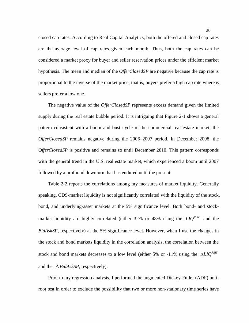
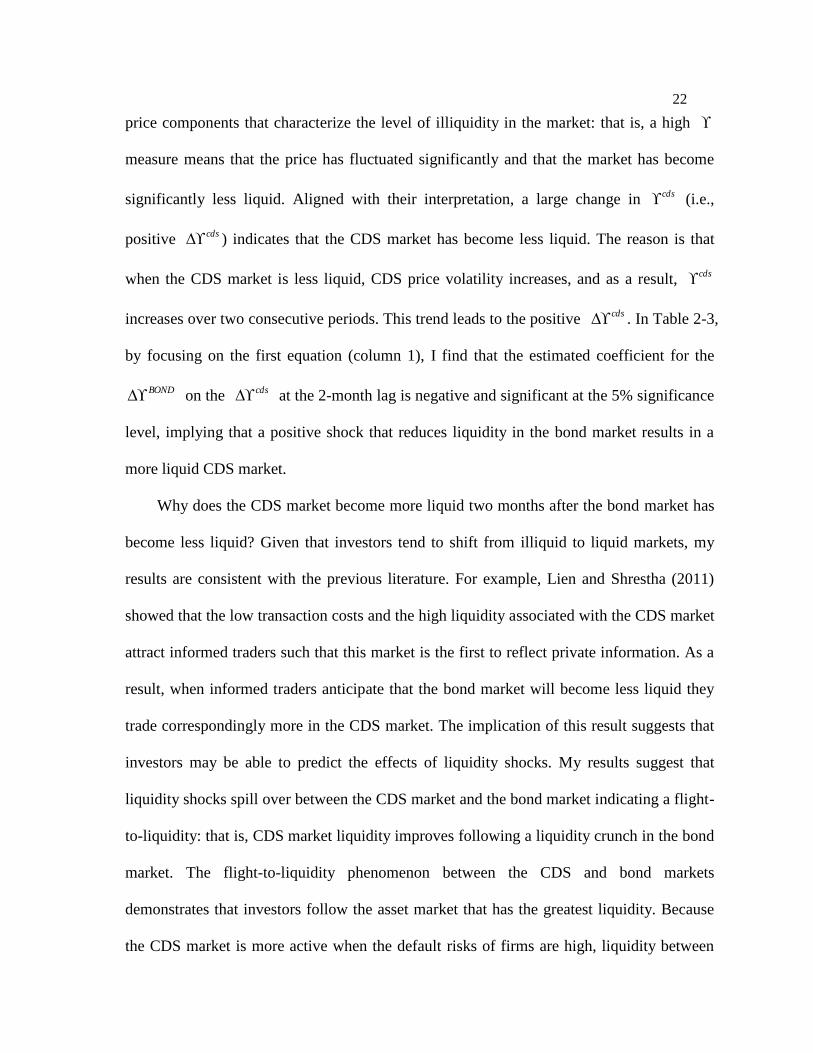
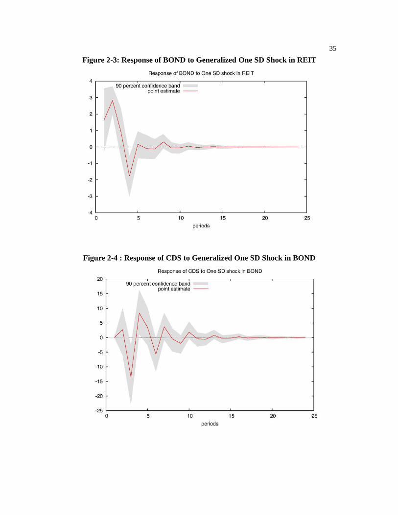
Figure 2-2 and Figure 2-3, respectively, depict the response of monthly changes in
bond-market liquidity to unit shocks in stock-market liquidity and vice versa. As I predicted
based on the VAR and Granger Causality analysis, the stock and bond markets show
evidence of a mutual feedback effect. One standard deviation change in bond-market
liquidity increases stock-market liquidity after one month and induces a decrease in stock-
market liquidity one month later. Subsequently, stock-market liquidity increases for the
next two months followed by a decrease in the third month. This pattern repeats until the
response of stock-market liquidity tapers to zero. Furthermore, one standard deviation
change in stock-market liquidity increases bond-market liquidity after one month and
induces a decrease in stock-market liquidity in each of the next two months. Subsequently,

27
bond-market liquidity repeats the trend whereby an increase in one month is followed by a
decrease in the next month. In the long run, this trend tapers to zero.
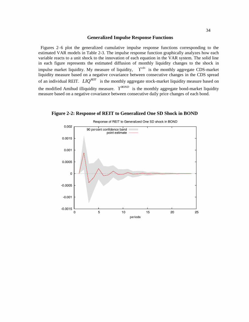
In Figure 2-4, it is evident that one month after one standard deviation change in bond-
market liquidity has taken place, CDS-market liquidity increases; however, after this initial
increase, CDS-market liquidity decreases in the following month. After this, CDS-market
liquidity increases in each of the next two months. Subsequently, CDS-market liquidity
repeats the trend whereby an increase in one month is followed by a decrease in the next
month, with this trend tapering to zero in the long run.
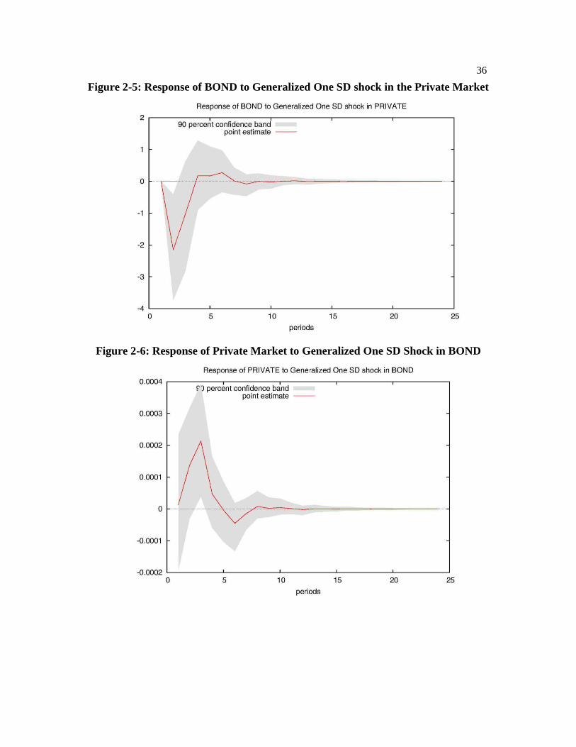
In Figure 2-5, one standard deviation change in the dSPOfferClose results in a
decrease in BOND after the first period, followed by a large spike in the response of the
BOND for the next period. After the third period, the response of bond-market liquidity is
insignificant, and in the long term the response of bond-market liquidity to the shock to
underlying-asset market liquidity diminishes to zero.
In Figure 2-6, one standard deviation change in theBOND leads to an increase in the
dSPOfferClose for the first two periods and then a decrease in each of the next two
periods. After these initial movements, the response of the underlying-asset liquidity tapers
to zero. Consistent with Bao, Pan, and Wang (2011), both BOND and
cds capture the
transitory impact of a liquidity shock on the market rather than its fundamental impact.
Variance Decomposition
Variance decomposition analysis helps me to see which portion of each variable’s
forecast error can be explained by the shocks from the rest of the variables. Overall, the
variance decomposition results show that liquidity fluctuation in each market originates

28
from its own shocks. However, liquidity shocks in one market have a significant
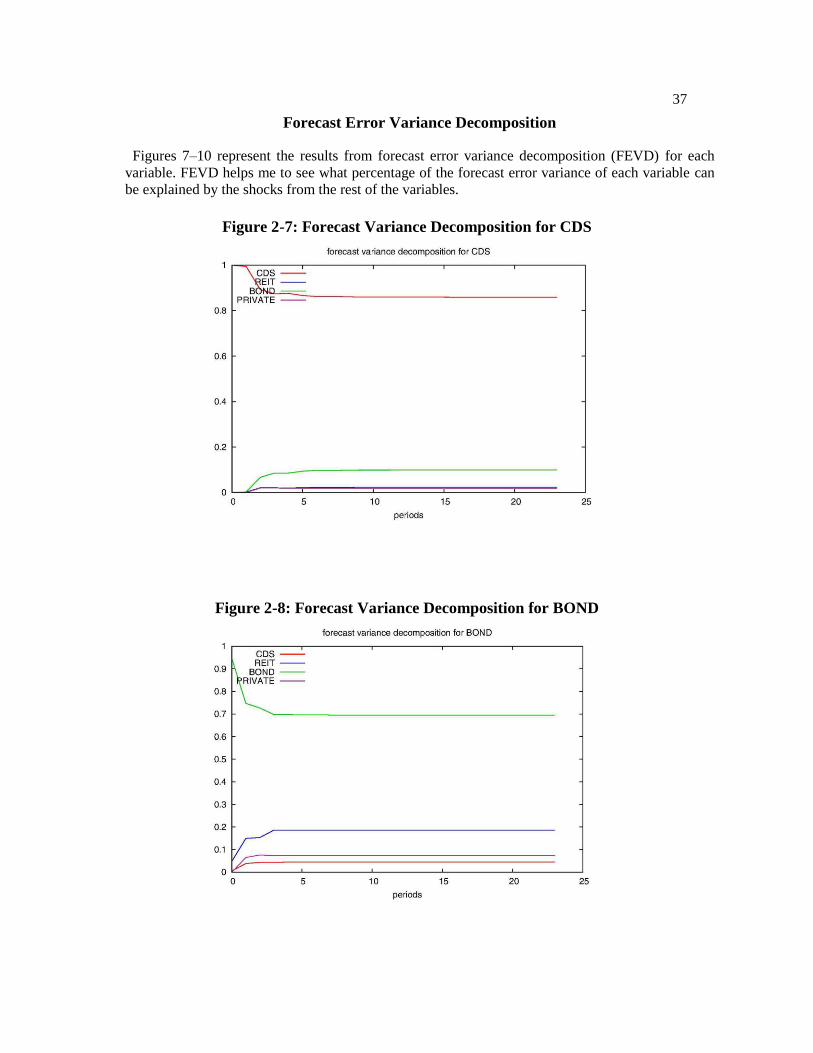
interdependent effect on other markets in the long run. Table 2-5 and Figure 2-7 present
data suggesting that a shock to bond-market liquidity is a significant source of liquidity
fluctuation in the CDS market, accounting for 9.9% of the shocks in the CDS market after
24 months, whereas its own shocks accounted for 85.9%, and the effects from liquidity
shocks in both the stock market and the underlying-asset market are relatively minor, such
as 2.37% and 1.82%, respectively.
The data presented in Table 2-6 and Figure 2-8 suggest that liquidity shocks to the
stock market are a very important source of fluctuations in bond-market liquidity as are the
bond market’s own shocks. Specifically, 18.64% of the bond-market liquidity shocks after
four months are due to stock-market liquidity shocks. Another explanatory source of
fluctuation in bond-market liquidity originates from underlying-asset liquidity, which
accounts for 7.3% of the bond-market liquidity shocks after four months. Liquidity shocks
to the CDS market play a minor role (4.34%) in bond-market liquidity fluctuations. The
impact of its own shocks on bond-market liquidity accounts for 69.71% and remain a major
source of its own fluctuations.
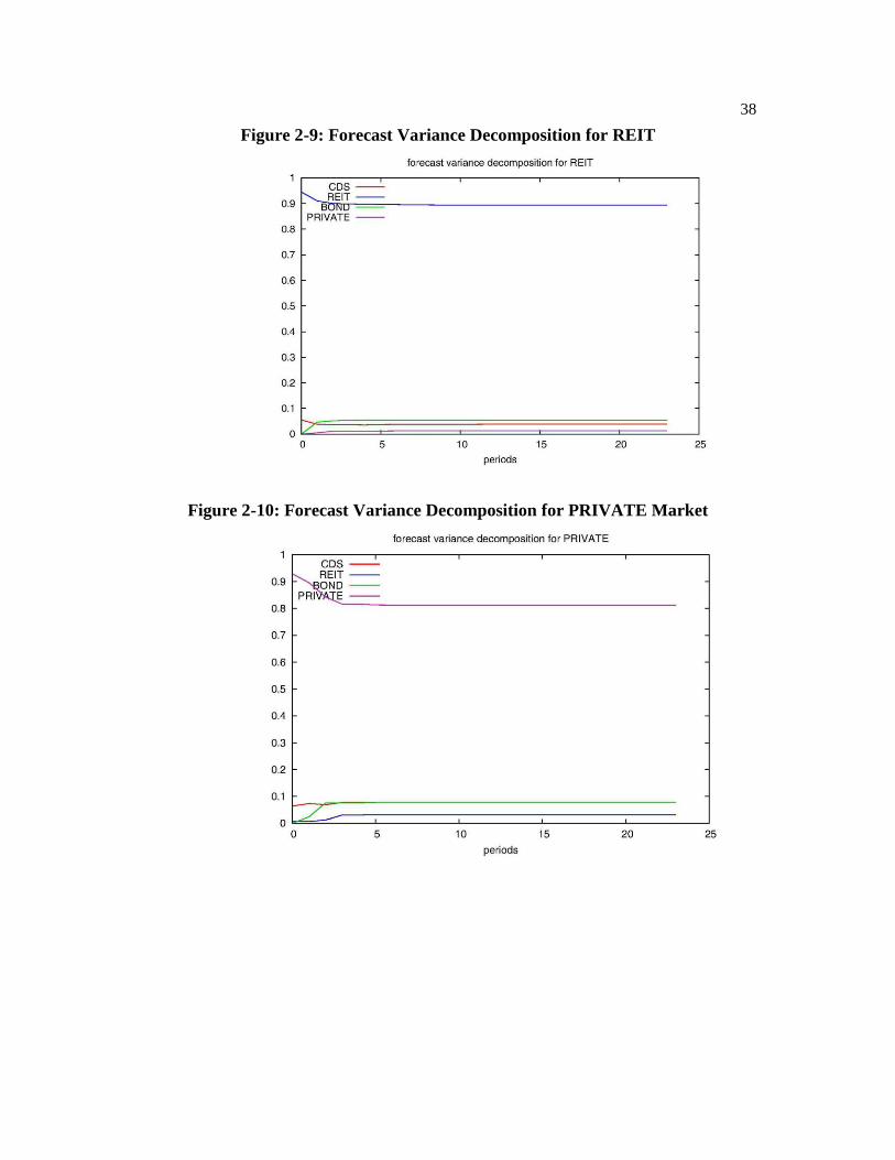
Table 2-7 and Figure 2-9 show that stock-market liquidity fluctuates mainly due to its
own shocks. A shock to stock market liquidity accounts for 89% of its own variance in the
forecast errors after 24 months, whereas bond-, stock-, and underlying-asset-market
liquidity accounts for 5.49%, 3.84%, and 1.24% of stock market liquidity fluctuation,
respectively. This result implies that the significance of underlying-asset liquidity for stock-
market liquidity may be limited. Table 2-8 and Figure 2-10 suggest that underlying-asset
liquidity fluctuates through both CDS- and bond-market liquidity channels. After four

29
months, CDS market liquidity accounts for 7.78% of forecast error variance in underlying-
asset liquidity, whereas bond-market liquidity accounts for 7.56%. The shocks to stock-
market liquidity have only a minor impact (3%).
In conclusion, other than its own shocks, after four months approximately 19% of the
fluctuation in bond-market liquidity can be explained by liquidity shocks originating in the
stock market. This result suggests that bond-market liquidity fluctuates mainly due to
liquidity shocks in the stock market. Shocks to underlying-asset liquidity also have a
moderate impact on fluctuations in bond-market liquidity such that 7% of the fluctuation in
bond-market liquidity can be explained by liquidity shocks from the underlying-asset
market. CDS-market liquidity fluctuates along with the shocks from bond-market liquidity
in the long run. Underlying-asset liquidity fluctuates due to shocks from both CDS- and
bond-market liquidity.
Robustness Check
I conduct a number of robustness exercises by employing different liquidity measures
and adding exogenous variables. As I expected, the main results are consistent with the
previous findings. In Table 2-9, instead of the OfferClosedSP, theCapRateSP is shown
as a proxy for underlying-asset liquidity. The CapRateSP is constructed as the difference
between the average cap rate and a 10-year Treasury bill rate. In the fourth equation
(column 4) in Table 2-9, bond-market liquidity negatively affects CDS-market liquidity. In
the second and third equations (columns 2 and 3) in Table 2-9, stock-market liquidity
positively affects bond-market liquidity with a 2-month lag whereas the bond-market effect
on the stock market is no longer substantial.

30
I find that the reason for this weaker relation between the bond and stock markets
arises from the effect of underlying asset market. In the fourth equation (column 4) in Table
2-9, the estimated coefficient for the BOND on the CapRateSP at a 1-month lag is
positive at the 1% significance level. Accordingly, I posit that the strong connection
between bond-market and underlying-asset liquidity dilutes the impact of bond-market
liquidity on stock-market liquidity.
In Table 2-10, the BidAskSP is used as a proxy for stock-market liquidity instead of
the REITLIQ . The BidAskSP is constructed as the aggregated average of the monthly
quoted spread for each stock based on the close–ask price and the bid price from the CRSP
daily database. In the third equation (column 3) in Table 2-10, stock-market liquidity is
shown to positively affect bond-market liquidity as the previous analysis suggested.
However, the relation does not hold vice versa. The liquidity spill-over between the bond
market and the CDS market still holds, as shown previously.
Finally, I test the robustness of my results by extending the previous VAR regression
through the addition of exogenous variables. The interest rate affects the general economic
condition of the market. Thus, I added a 5-year Treasury bill yield as an exogenous variable
to the existing VAR model in order to control general economic conditions. Overall, despite
the addition of exogenous variables, the main results hold as before. In the second and third
equations (column 2 and 3) of Table 2-11, stock-market liquidity positively affects bond-
market liquidity at the 1-month and 2-month lag.

31
Summary of Findings
Considerable anecdotal evidence suggests that the effects of liquidity shocks spread
quickly throughout the financial sector. This paper examines the liquidity spill-over impact
across real estate capital markets: the stock (REIT) market, the derivative (CDS) market,
and the corporate-bond market, and the private (property sale–based) market. Given the
fundamental link between the underlying assets of the public and private real estate markets,
liquidity shocks are more likely to spill over across these particular markets.
My study contributes to the existing literature by concentrating on the dynamics of
liquidity between the private and public real estate markets. The analysis of liquidity-shock
patterns across the different real estate markets has important implications for investor asset
allocation and portfolio management models. Specifically, I show that liquidity shocks have
interdependent effects on the private and public markets. Investors in possession of such
knowledge could refine their risk-management strategies accordingly and manage their
portfolios based on correspondingly better predictions of the liquidity patterns across real
estate markets.
Using VAR, I investigated liquidity-shock spill-over across the four markets. The
VAR results show that bond-market liquidity shocks negatively impact CDS market
liquidity with a 2-month lag. Furthermore, a stock-market liquidity shock Granger Causes
bond-market liquidity with a 2-month lag. Underlying asset liquidity (private-market
liquidity) Granger Causes bond-market liquidity and the relation holds vice versa. However,
the spill-over impact of underlying asset liquidity on the public real-estate market varies in
accordance with different measures.
Variance decomposition analysis implies that bond-market liquidity fluctuates mainly

32
due to the liquidity shocks in the stock market. Shocks to underlying-asset liquidity also
have a moderate impact on fluctuations in bond-market liquidity. CDS-market liquidity
fluctuates along with the shocks from bond-market liquidity in the long run. Underlying-
asset liquidity fluctuates due to shocks from CDS-market liquidity and from bond-market
liquidity.
In future research, I will focus on determining the factors that cause the feedback
impact between stock- and bond-market liquidity. Furthermore, I will test the factors that
cause the negative impact of bond-market liquidity on CDS-market liquidity. Consistent
with the previous literature, I conjecture that the private information available to investors
in each market plays a role in creating different spill-over liquidity-shock patterns across
real estate markets. Further research is required to test this information hypothesis in order
to investigate the dynamics of liquidity shocks across real estate markets.

33
Figure 2-1: Monthly Time-Series of the dSPOfferClose
The dSPOfferClose is the aggregate average difference between the offered and closed cap rates
across four property types (apartment, industry, office, and retail).
34
Generalized Impulse Response Functions
Figures 2–6 plot the generalized cumulative impulse response functions corresponding to the
estimated VAR models in Table 2-3. The impulse response function graphically analyzes how each
variable reacts to a unit shock to the innovation of each equation in the VAR system. The solid line
in each figure represents the estimated diffusion of monthly liquidity changes to the shock in
impulse market liquidity. My measure of liquidity, cds is the monthly aggregate CDS-market
liquidity measure based on a negative covariance between consecutive changes in the CDS spread
of an individual REIT. REITLIQ is the monthly aggregate stock-market liquidity measure based on
the modified Amihud illiquidity measure. BOND is the monthly aggregate bond-market liquidity
measure based on a negative covariance between consecutive daily price changes of each bond.
Figure 2-2: Response of REIT to Generalized One SD Shock in BOND
35
Figure 2-3: Response of BOND to Generalized One SD Shock in REIT
Figure 2-4 : Response of CDS to Generalized One SD Shock in BOND
36
Figure 2-5: Response of BOND to Generalized One SD shock in the Private Market
Figure 2-6: Response of Private Market to Generalized One SD Shock in BOND
37
Forecast Error Variance Decomposition
Figures 7–10 represent the results from forecast error variance decomposition (FEVD) for each
variable. FEVD helps me to see what percentage of the forecast error variance of each variable can
be explained by the shocks from the rest of the variables.
Figure 2-7: Forecast Variance Decomposition for CDS
Figure 2-8: Forecast Variance Decomposition for BOND
38
Figure 2-9: Forecast Variance Decomposition for REIT
Figure 2-10: Forecast Variance Decomposition for PRIVATE Market
39
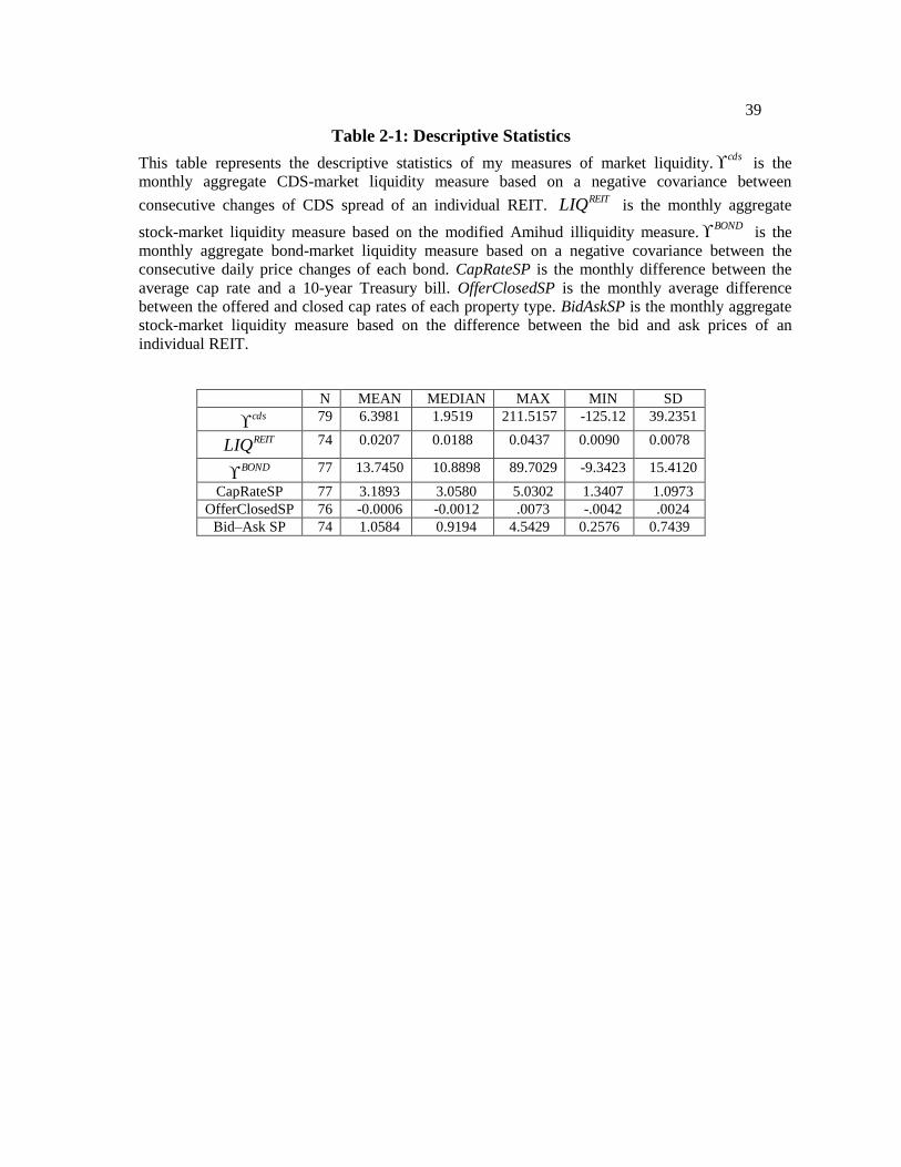
Table 2-1: Descriptive Statistics
This table represents the descriptive statistics of my measures of market liquidity.cds is the
monthly aggregate CDS-market liquidity measure based on a negative covariance between
consecutive changes of CDS spread of an individual REIT. REITLIQ is the monthly aggregate
stock-market liquidity measure based on the modified Amihud illiquidity measure.BOND is the
monthly aggregate bond-market liquidity measure based on a negative covariance between the
consecutive daily price changes of each bond. CapRateSP is the monthly difference between the
average cap rate and a 10-year Treasury bill. OfferClosedSP is the monthly average difference
between the offered and closed cap rates of each property type. BidAskSP is the monthly aggregate
stock-market liquidity measure based on the difference between the bid and ask prices of an
individual REIT.
N MEAN MEDIAN MAX MIN SD
cds
79 6.3981 1.9519 211.5157 -125.12 39.2351
REITLIQ 74 0.0207 0.0188 0.0437 0.0090 0.0078
BOND 77 13.7450 10.8898 89.7029 -9.3423 15.4120
CapRateSP 77 3.1893 3.0580 5.0302 1.3407 1.0973
OfferClosedSP 76 -0.0006 -0.0012 .0073 -.0042 .0024
Bid–Ask SP 74 1.0584 0.9194 4.5429 0.2576 0.7439

40
Table 2-2: Correlations
This table reports the contemporaneous correlations of my measures of market liquidity.cds is the
monthly aggregate CDS-market liquidity measure based on a negative covariance between
consecutive changes of the CDS spread of an individual REIT.REITLIQ is the monthly aggregate
stock-market liquidity measure based on the modified Amihud illiquidity measure.BOND is the
monthly aggregate bond-market liquidity measure based on a negative covariance between
consecutive daily price changes of each bond. CapRateSP is the monthly difference between the
average cap rate and a 10-year Treasury bill. OfferClosedSP is the monthly average difference
between the offered and closed cap rates of each property type. BidAskSP is the monthly aggregate
stock-market liquidity measure based on the difference between the bid and ask prices of an
individual REIT.
cds BOND
REITLIQ Bid–AskSP OfferClosedSP CapRateSP
cds
1
BOND 0.0504 1
REITLIQ 0.0864 0.3234** 1
Bid–AskSP 0.1863 0.4832** 0.3130** 1
OfferClosedSP -0.1308 -0.0407 -0.0179 -0.4075** 1
CapRateSP -0.0791 0.0677 -0.3910** -0.3283** 0.5796** 1
* p < 0.1, ** p < 0.05, *** p < 0.01

41
Table 2-3: VAR using the OfferClosedSP with 2-month lag
This table represents the results from estimating four unrestricted VAR models for the underlying-
asset, CDS, bond, and stock markets. An unrestricted thp -order Gaussian VAR model can be
represented as
tptpttt eYYYY 2211=
The lag-length of the VAR is chosen by looking at the FPE, AIC, HQIC, SBIC, and the likelihood
ratio for various choices of p. My measure of liquidity,cds , is the monthly aggregate CDS-market
liquidity measure based on a negative covariance between consecutive changes of the CDS spread
of an individual REIT. REITLIQ is the monthly aggregate stock-market liquidity measure based on
the modified Amihud illiquidity measure. BOND is the monthly aggregate bond-market liquidity
measure based on a negative covariance between the consecutive daily price changes of each bond.
OfferClosedSP is the monthly average difference between the offered and closed cap rates of each
property type. MonthlyDummy constitutes a system of dummy variables defined by the months of
the year. CrisisDum is a dummy variable with the value 1 for a sub-period before 2008 and
otherwise, 0. (t statistics in parentheses, * p < 0.1, ** p < 0.05, *** p < 0.01)
cds
t REIT
tLIQ BOND
t tdSPOfferClose
cds
t 1 -0.814***
(-6.82)
0.00000979
(0.97)
0.00849
(0.38)
-0.00000195
(-0.74)
cds
t 2 -0.511***
(-4.28)
0.00000573
(0.57)
0.00104
(0.05)
-0.00000175
(-0.67)
REIT
tLIQ 1 568.1
(0.36) -0.744
***
(-5.54) 767.2
**
(2.55)
-0.0120
(-0.34)
REIT
tLIQ 2 -522.2
(-0.33) -0.350
**
(-2.61) 791.6
**
(2.64)
-0.0128
(-0.37)
BOND
t 1 0.375
(0.54) 0.000122
**
(2.08)
0.0921
(0.70)
0.0000186
(1.22)
BOND
t 2 -1.648**
(-2.45)
0.0000173
(0.30)
-0.200
(-1.57) 0.0000277
*
(1.87)
1 tdSPOfferClose -1350.7
(-0.21)
0.344
(0.63) -2576.4
**
(-2.12)
0.106
(0.75)
2 tdSPOfferClose 8665.4
(1.28)
0.119
(0.21)
-963.2
(-0.75)
0.0829
(0.56)
CRISISDUM 3.187
(0.28)
0.0000210
(0.02)
-0.605
(-0.28)
-0.000180
(-0.71)
Constant 6.117
(0.28)
-0.00213
(-1.15)
-0.272
(-0.07)
0.0000898
(0.19)
MonthlyDummy Yes Yes Yes Yes
Observations 69
2R 0.62 0.53 0.44 0.26
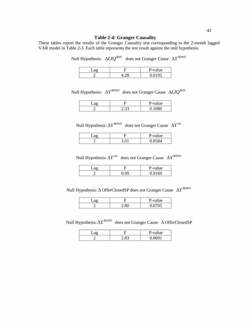
42
Table 2-4: Granger Causality These tables report the results of the Granger Causality test corresponding to the 2-month lagged
VAR model in Table 2-3. Each table represents the test result against the null hypothesis.
Null Hypothesis: REITLIQ does not Granger Cause
BOND
Lag F P-value
2 4.28 0.0195
Null Hypothesis: BOND does not Granger Cause
REITLIQ
Lag F P-value
2 2.33 0.1080
Null Hypothesis:BOND does not Granger Cause
cds
Lag F P-value
2 3.01 0.0584
Null Hypothesis:cds does not Granger Cause
BOND
Lag F P-value
2 0.09 0.9160
Null Hypothesis:OfferClosedSP does not Granger Cause BOND
Lag F P-value
2 2.80 0.0705
Null Hypothesis:BOND does not Granger Cause OfferClosedSP
Lag F P-value
2 2.83 0.0691

43
Forecast Error Variance Decomposition
Tables 5–8 represent the results from the forecast error variance decomposition (FEVD) for each
variable. FEVD helps us to see the percentage of each variable’s forecast error variance that can be
explained by the shocks from the rest of the variables.
Table 2-5: Decomposition of Variance for CDS
t
period std.error CDS
t REIT
tLIQ BOND
t tdSPOfferClose
1 39.459 100.0000 0.0000 0.0000 0.0000
2 50.4271 99.4052 0.2560 0.2885 0.0503
3 53.2905 89.2363 2.0975 6.6875 1.9786
4 55.0763 87.3847 2.0664 8.5759 1.9730
5 56.3726 87.5728 1.9738 8.5689 1.8844
6 56.9558 86.6251 2.1302 9.3986 1.8461
7 57.1415 86.1922 2.2118 9.7498 1.8461
8 57.2996 86.2575 2.2025 9.7032 1.8367
9 57.3995 86.1159 2.2598 9.7935 1.8309
10 57.4517 85.9608 2.3296 9.8820 1.8276
11 57.4725 85.9556 2.3377 9.8803 1.8264
12 57.486 85.9444 2.3438 9.8861 1.8257
13 57.4959 85.9147 2.3610 9.8992 1.8250
14 57.5005 85.9086 2.3662 9.9003 1.8248
15 57.5023 85.9084 2.3662 9.9006 1.8248
16 57.5038 85.9039 2.3686 9.9028 1.8247
17 57.5047 85.9022 2.3700 9.9031 1.8247
18 57.505 85.9022 2.3700 9.9030 1.8247
19 57.5053 85.9017 2.3703 9.9034 1.8247
20 57.5054 85.9013 2.3705 9.9035 1.8247
21 57.5055 85.9013 2.3705 9.9035 1.8247
22 57.5055 85.9012 2.3706 9.9035 1.8247
23 57.5056 85.9012 2.3706 9.9035 1.8247
24 57.5056 85.9012 2.3706 9.9035 1.8247
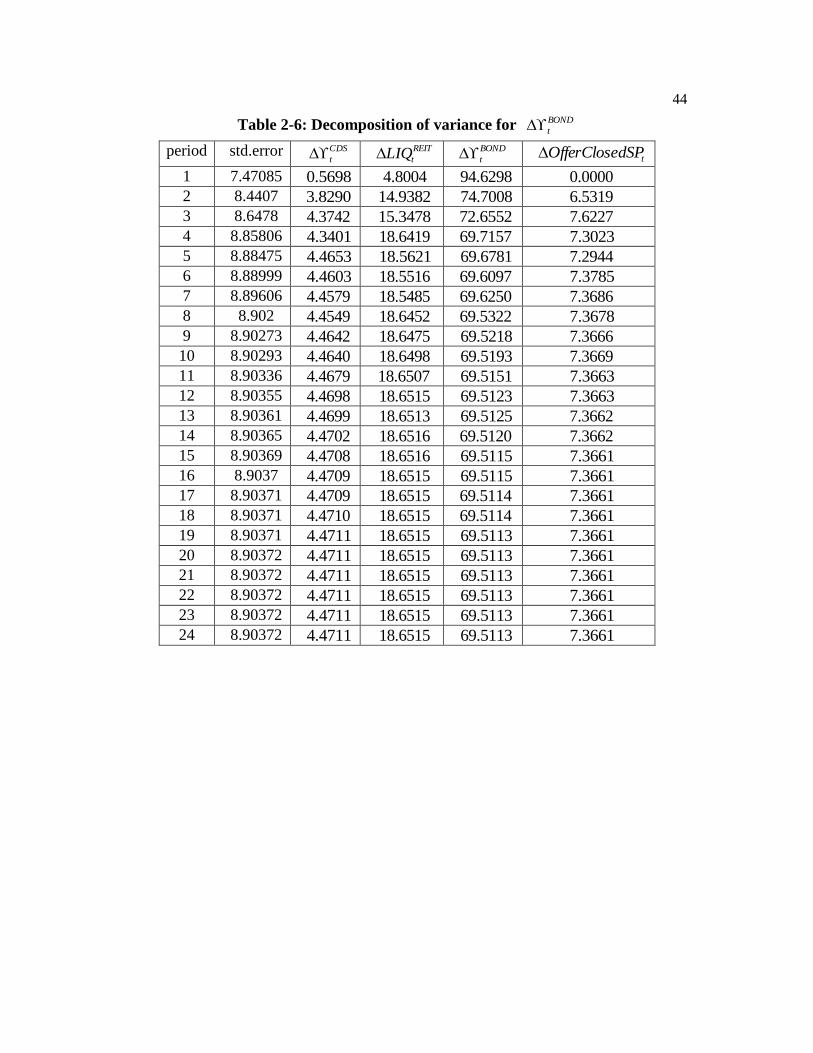
44
Table 2-6: Decomposition of variance for BOND
t
period std.error CDS
t REIT
tLIQ BOND
t tdSPOfferClose
1 7.47085 0.5698 4.8004 94.6298 0.0000
2 8.4407 3.8290 14.9382 74.7008 6.5319
3 8.6478 4.3742 15.3478 72.6552 7.6227
4 8.85806 4.3401 18.6419 69.7157 7.3023
5 8.88475 4.4653 18.5621 69.6781 7.2944
6 8.88999 4.4603 18.5516 69.6097 7.3785
7 8.89606 4.4579 18.5485 69.6250 7.3686
8 8.902 4.4549 18.6452 69.5322 7.3678
9 8.90273 4.4642 18.6475 69.5218 7.3666
10 8.90293 4.4640 18.6498 69.5193 7.3669
11 8.90336 4.4679 18.6507 69.5151 7.3663
12 8.90355 4.4698 18.6515 69.5123 7.3663
13 8.90361 4.4699 18.6513 69.5125 7.3662
14 8.90365 4.4702 18.6516 69.5120 7.3662
15 8.90369 4.4708 18.6516 69.5115 7.3661
16 8.9037 4.4709 18.6515 69.5115 7.3661
17 8.90371 4.4709 18.6515 69.5114 7.3661
18 8.90371 4.4710 18.6515 69.5114 7.3661
19 8.90371 4.4711 18.6515 69.5113 7.3661
20 8.90372 4.4711 18.6515 69.5113 7.3661
21 8.90372 4.4711 18.6515 69.5113 7.3661
22 8.90372 4.4711 18.6515 69.5113 7.3661
23 8.90372 4.4711 18.6515 69.5113 7.3661
24 8.90372 4.4711 18.6515 69.5113 7.3661
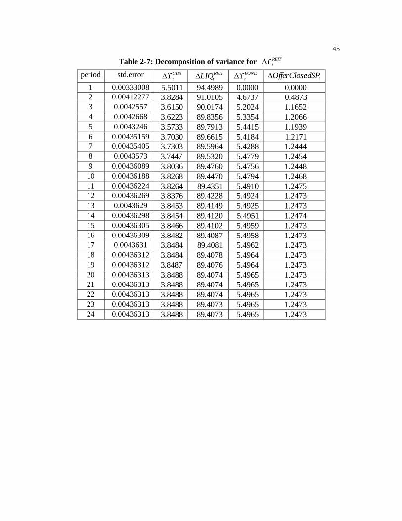
45
Table 2-7: Decomposition of variance for REIT
t
period std.error CDS
t REIT
tLIQ BOND
t tdSPOfferClose
1 0.00333008 5.5011 94.4989 0.0000 0.0000
2 0.00412277 3.8284 91.0105 4.6737 0.4873
3 0.0042557 3.6150 90.0174 5.2024 1.1652
4 0.0042668 3.6223 89.8356 5.3354 1.2066
5 0.0043246 3.5733 89.7913 5.4415 1.1939
6 0.00435159 3.7030 89.6615 5.4184 1.2171
7 0.00435405 3.7303 89.5964 5.4288 1.2444
8 0.0043573 3.7447 89.5320 5.4779 1.2454
9 0.00436089 3.8036 89.4760 5.4756 1.2448
10 0.00436188 3.8268 89.4470 5.4794 1.2468
11 0.00436224 3.8264 89.4351 5.4910 1.2475
12 0.00436269 3.8376 89.4228 5.4924 1.2473
13 0.0043629 3.8453 89.4149 5.4925 1.2473
14 0.00436298 3.8454 89.4120 5.4951 1.2474
15 0.00436305 3.8466 89.4102 5.4959 1.2473
16 0.00436309 3.8482 89.4087 5.4958 1.2473
17 0.0043631 3.8484 89.4081 5.4962 1.2473
18 0.00436312 3.8484 89.4078 5.4964 1.2473
19 0.00436312 3.8487 89.4076 5.4964 1.2473
20 0.00436313 3.8488 89.4074 5.4965 1.2473
21 0.00436313 3.8488 89.4074 5.4965 1.2473
22 0.00436313 3.8488 89.4074 5.4965 1.2473
23 0.00436313 3.8488 89.4073 5.4965 1.2473
24 0.00436313 3.8488 89.4073 5.4965 1.2473
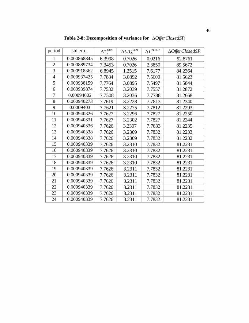
46
Table 2-8: Decomposition of variance for tdSPOfferClose
period std.error CDS
t REIT
tLIQ BOND
t tdSPOfferClose
1 0.000868845 6.3998 0.7026 0.0216 92.8761
2 0.000889734 7.3453 0.7026 2.3850 89.5672
3 0.000918362 6.8945 1.2515 7.6177 84.2364
4 0.000937425 7.7884 3.0892 7.5600 81.5623
5 0.000938159 7.7764 3.0895 7.5497 81.5844
6 0.000939874 7.7532 3.2039 7.7557 81.2872
7 0.00094002 7.7508 3.2036 7.7788 81.2668
8 0.000940273 7.7619 3.2228 7.7813 81.2340
9 0.0009403 7.7621 3.2275 7.7812 81.2293
10 0.000940326 7.7627 3.2296 7.7827 81.2250
11 0.000940331 7.7627 3.2302 7.7827 81.2244
12 0.000940336 7.7626 3.2307 7.7833 81.2235
13 0.000940338 7.7626 3.2309 7.7832 81.2233
14 0.000940338 7.7626 3.2309 7.7832 81.2232
15 0.000940339 7.7626 3.2310 7.7832 81.2231
16 0.000940339 7.7626 3.2310 7.7832 81.2231
17 0.000940339 7.7626 3.2310 7.7832 81.2231
18 0.000940339 7.7626 3.2310 7.7832 81.2231
19 0.000940339 7.7626 3.2311 7.7832 81.2231
20 0.000940339 7.7626 3.2311 7.7832 81.2231
21 0.000940339 7.7626 3.2311 7.7832 81.2231
22 0.000940339 7.7626 3.2311 7.7832 81.2231
23 0.000940339 7.7626 3.2311 7.7832 81.2231
24 0.000940339 7.7626 3.2311 7.7832 81.2231

47
Table 2-9: VAR using the CapRateSP with a 2-month lag
This table represents the results from estimating four unrestricted VAR models for the underlying-asset, CDS,
bond, and stock markets. An unrestricted thp -order Gaussian VAR model can be represented as
tptpttt eYYYY 2211=
The lag length of the VAR is chosen by looking at the FPE, AIC, HQIC, and SBIC, as well as the likelihood
ratio for various choices of p. My measure of liquidity, cds , is the monthly aggregate CDS-market liquidity
measure based on a negative covariance between consecutive changes of the CDS spread of an individual
REIT. REITLIQ is the monthly aggregate stock-market liquidity measure based on the modified Amihud
illiquidity measure. BOND is the monthly aggregate bond-market liquidity measure based on a negative
covariance between the consecutive daily price changes of each bond. CapRateSP is the monthly difference
between the average cap rate and a 10-year Treasury bill. MonthlyDummy constitutes a system of dummy
variables defined by the months of the year. CrisisDum is a dummy variable with the value 1 for a sub-period
before 2008 and otherwise, 0. (t statistics in parentheses * p < 0.1, ** p < 0.05, *** p < 0.01)
cds
t REIT
tLIQ BOND
t tCapRateSP
cds
t 1 -0.827***
(-6.92)
0.00000458
(0.44)
0.0143
(0.60)
-0.000218
(-0.36)
cds
t 2 -0.536***
(-4.57)
0.00000154
(0.15)
0.0122
(0.53)
-0.000897
(-1.49)
REIT
tLIQ 1 1137.1
(0.71) -0.702
***
(-5.10) 620.7
*
(1.97)
8.382
(1.03)
REIT
tLIQ 2 -118.9
(-0.08) -0.331
**
(-2.54) 682.9
**
(2.29)
3.917
(0.51)
BOND
t 1 -0.0584
(-0.09)
0.0000944
(1.63)
0.106
(0.80) 0.0127
***
(3.70)
BOND
t 2 -1.739**
(-2.24)
0.0000185
(0.28)
-0.125
(-0.81)
0.00513
(1.29)
1 tCapRateSP 0.353
(0.01)
0.000734
(0.29)
-7.147
(-1.25)
0.207
(1.39)
2 tCapRateSP -17.78
(-0.69)
-0.00207
(-0.93)
-3.086
(-0.60)
0.0161
(0.12)
cons 11.07
(0.54)
-0.00214
(-1.20)
-0.968
(-0.24)
-0.00637
(-0.06)
MonthlyDummy Yes Yes Yes Yes
N 71 2R
0.61 0.52 0.37 0.44

48
Table 2-10: VAR using the BidAskSP with a 2-month lag This table shows the results from estimating four unrestricted VAR models for the underlying-asset, CDS,
bond, and stock markets. An unrestricted thp -order Gaussian VAR model can be represented as
tptpttt eYYYY 2211=
The lag-length of the VAR is chosen by looking at the FPE, AIC, HQIC, and SBIC, as well as the likelihood
ratio for various choices of p. My measure of liquidity, cds is the monthly aggregate CDS-market liquidity
measure based on a negative covariance between consecutive changes of the CDS spread of an individual
REIT. BOND is the monthly aggregate bond-market liquidity measure based on a negative covariance
between the consecutive daily price changes of each bond. CapRateSP is the monthly difference between the
average cap rate and a 10-year Treasury bill. The BidAskSP is the monthly aggregate stock-market liquidity
measure based on the difference between the bid and ask prices of an individual REIT. MonthlyDummy
constitutes a system of dummy variables defined by the months of the year. CrisisDum is a dummy variable
with the value 1 for a sub-period before 2008 and the value of 0 otherwise. (t statistics in parentheses, * p <0.1, ** p < 0.05, *** p < 0.01)
cds
t tBidAskSP BOND
t tCapRateSP
cds
t 1 -0.820***
(-6.98)
0.00151
(1.10)
0.0108
(0.55)
0.000104
(0.18)
cds
t 2 -0.544***
(-4.63)
0.000618
(0.45)
0.00242
(0.12)
-0.000526
(-0.92)
1 tBidAskSP 8.623
(0.78) -0.269
**
(-2.09) 7.985
***
(4.36) -0.133
**
(-2.48)
2 tBidAskSP 5.975
(0.47) -0.480
***
(-3.23) 8.430
***
(4.00)
-0.00806
(-0.13)
BOND
t 1 -0.142
(-0.19)
0.00726
(0.83)
0.00265
(0.02) 0.0121
***
(3.33)
BOND
t 2 -1.538**
(-2.11)
0.00233
(0.27)
-0.0527
(-0.43) 0.00659
*
(1.84)
1 tCapRateSP -2.832
(-0.10) -0.755
**
(-2.22)
-1.496
(-0.31)
0.146
(1.03)
2 tCapRateSP -11.83
(-0.46)
0.0709
(0.23)
-2.232
(-0.52)
-0.000797
(-0.01)
Constant 12.23
(0.59)
-0.200
(-0.81)
2.597
(0.75)
-0.0650
(-0.64)
MonthlyDummy Yes Yes Yes Yes
N 71 2R
0.60 0.32 0.56 0.49

49
Table 2-11: VAR using the 5YR Treasury-Bill with a 2-month lag This table represents results from estimating four unrestricted VAR models for the underlying-asset, CDS,
bond, and stock markets. An unrestricted thp order Gaussian VAR model can be represented as:
tptpttt eYYYY 2211=
The lag length of the VAR is chosen by looking at the FPE, AIC, HQIC, and SBIC, as well as the likelihood
ratio for various choices of p. My measure of liquidity, cds , is the monthly aggregate CDS-market liquidity
measure based on a negative covariance between consecutive changes of the CDS spread of an individual
REIT. REITLIQ is the monthly aggregate stock-market liquidity measure based on the modified Amihud
illiquidity measure. BOND is the monthly aggregate bond-market liquidity measure based on a negative
covariance between the consecutive daily price changes of each bond. OfferClosedSP is the monthly average
difference between the offered and closed cap rates of each property type. MonthlyDummy constitutes a
system of dummy variables defined by the months of the year. CrisisDum is a dummy variable with the value
1 for a sub-period before 2008 and otherwise, 0. 5YRTBILL is the 5-year Treasury bill yield. (t statistics in
parentheses, * p < 0.1, ** p < 0.05, *** p < 0.01)
cds
t REIT
tLIQ BOND
t tdSPOfferClose
cds
t 1 -0.814***
(-6.75)
0.00000990
(0.98)
0.00934
(0.43)
-0.00000191
(-0.73)
cds
t 2 -0.511***
(-4.24)
0.00000552
(0.54)
-0.000487
(-0.02)
-0.00000183
(-0.69)
REIT
tLIQ 1 558.8
(0.35) -0.755
***
(-5.55) 686.9
**
(2.37)
-0.0160
(-0.45)
REIT
tLIQ 2 -530.1
(-0.33) -0.359
**
(-2.65) 722.3
**
(2.50)
-0.0162
(-0.46)
BOND
t 1 0.371
(0.52) 0.000117
*
(1.97)
0.0569
(0.45)
0.0000169
(1.10)
BOND
t 2 -1.644**
(-2.39)
0.0000222
(0.38)
-0.164
(-1.33) 0.0000295
*
(1.97)
1 tdSPOfferClose -1383.6
(-0.21)
0.305
(0.56) -2862.6
**
(-2.44)
0.0922
(0.65)
2 tdSPOfferClose 8640.6
(1.26)
0.0902
(0.16)
-1179.3
(-0.96)
0.0723
(0.48)
CRISISDUM 1.854
(0.06)
-0.00154
(-0.61) -12.20
**
(-2.26)
-0.000752
(-1.14)
5YRTBILL 0.612
(0.05)
0.000715
(0.67) 5.324
**
(2.33)
0.000262
(0.94)
Constant 4.919
(0.15)
-0.00353
(-1.26) -10.69
*
(-1.79)
-0.000424
(-0.58)
MonthlyDummy Yes Yes Yes Yes
Observations 69 2R
0.62 0.54 0.50 0.27
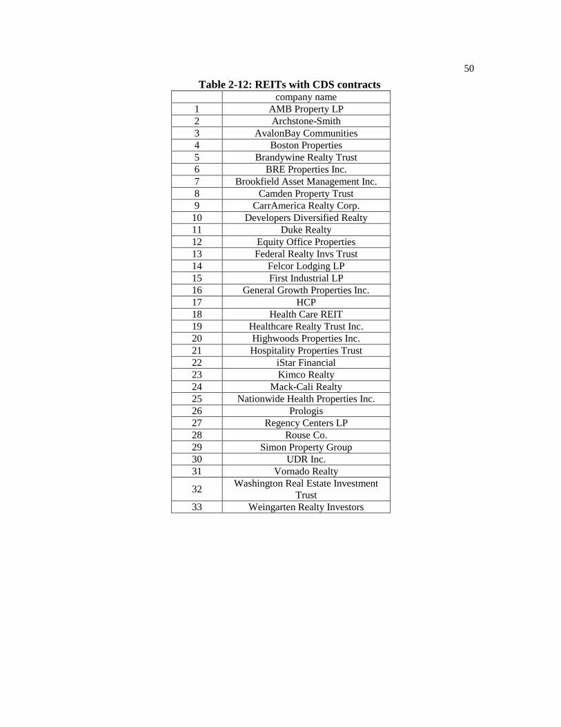
50
Table 2-12: REITs with CDS contracts company name
1 AMB Property LP
2 Archstone-Smith
3 AvalonBay Communities
4 Boston Properties
5 Brandywine Realty Trust
6 BRE Properties Inc.
7 Brookfield Asset Management Inc.
8 Camden Property Trust
9 CarrAmerica Realty Corp.
10 Developers Diversified Realty
11 Duke Realty
12 Equity Office Properties
13 Federal Realty Invs Trust
14 Felcor Lodging LP
15 First Industrial LP
16 General Growth Properties Inc.
17 HCP
18 Health Care REIT
19 Healthcare Realty Trust Inc.
20 Highwoods Properties Inc.
21 Hospitality Properties Trust
22 iStar Financial
23 Kimco Realty
24 Mack-Cali Realty
25 Nationwide Health Properties Inc.
26 Prologis
27 Regency Centers LP
28 Rouse Co.
29 Simon Property Group
30 UDR Inc.
31 Vornado Realty
32 Washington Real Estate Investment
Trust
33 Weingarten Realty Investors

51
Table 2-13: REITs with traded bonds company name
1 Camden Property Trust
2 Developers Diversified Realty
3 Duke Realty
4 Federal Realty Invs Trust
5 Healthcare Realty Trust Inc.
6 Nationwide Health Properties Inc.
7 Prologis
8 Simon Property Group
9 Vornado Realty
10 Washington Real Estate Investment
Trust
11 Archstone-Smith
12 BRE Properties Inc.
13 CarrAmerica Realty Corp.
14 HCP
15 Health Care REIT
16 Hospitality Properties Trust
17 iStar Financial
18 Kimco Realty
19 Rouse Co.
20 Weingarten Realty Investors

52
Chapter 3
Does the Law of One Price Hold in Heterogeneous Asset Markets?
A Test Using the U.S. Commercial Real Estate Market16
The law of one price (hereafter, LOOP) is one of the most fundamental assumptions in
finance theory. It is slightly more general than the absence of arbitrage.17
The law naturally
applies to relatively homogeneous goods such as wheat. It also extends to heterogeneous
goods when a unique implicit price function exists for each characteristic of a particular
good or asset. Rosen (1986) formalize the hedonic model describing the equilibrium in
heterogeneous goods markets by assuming market transactions between heterogeneous
buyers and sellers.
In the absence of market frictions, if arbitrageurs bring an asset’s price back to the
fundamental value, LOOP prevails. However, in practice, we observe a price discrepancy
when arbitrage is limited. Well-known examples are the price divergences that characterize
equity shares with multiple listings, such as Royal Dutch/Shell and Palm/3Com.18
In
response to the existence of mispricing in practice, researchers developed a theory
pertaining to the limits of arbitrage.19
The limits of arbitrage give rise to a central question: Why aren’t arbitrageurs able to
eliminate mispricing? Gromb and Vayanos (2010) survey a variety of potential answers to
this question. They argue that arbitrageurs face a variety of costs that prevent them from
16
This chapter is based on a paper co-authored with Jiro Yoshida. 17
See Pliska (1997) on the relation between the law of one price and the absence of arbitrage. 18
See Rosenthal and Young (1990) on Royal Dutch/Shell; see Lamont and Thaler (2003) on Palm/3Com. 19
See Gromb and Vayanos (2010) for a review.

53
eliminating mispricing: non-fundamental risk, holding costs, leverage constraints, and
equity constraints.
The commercial real estate market is also constrained by those costs, such that
arbitrage is limited. Agency friction between investment managers and clients can generate
a barrier to arbitrage. Additionally, it is not possible to short-sell properties in real estate
markets; therefore, we can assume that the holding costs of real estate assets are usually
larger than those of other financial assets. Buyers using mortgages to purchase houses are
constrained by leverage. If the equity size of a fund is not enough to purchase a building,
arbitrageurs in the commercial real estate market are constrained. Hence, my motivation for
this study starts with two closely related empirical questions: If the commercial real estate
market is not free from the limits of arbitrage, does market segmentation exist? If so, how is
the market segmented and what are the implications of this?
The objective of this study is to empirically test whether the law of one price holds in
an important class of heterogeneous assets: commercial real estate. More specifically, does
average pricing differ by investor type? If average pricing does not differ, does a given
asset have more than one factor price? If each investor transacts for the same asset but each
does so in a different domain, is the factor price of the heterogeneous assets discontinuous?
In considering answers to these research questions, I specify three types of market
segmentation (see Figure 3-3). With Type I market segmentation, investors, on average,
trade the same asset at different prices. In this case, we should observe systematic price
differences by investor type for comparable assets. I test average price differences by using
both the propensity score-matching estimation and pairwise hedonic regressions. With Type
II market segmentation, if average prices do not differ by investor type, then the marginal

54
factor prices for the average asset differ. I test for heterogeneous factor prices when
matching estimation results do not show a significant price difference. With Type III
market segmentation, matching is not feasible because investors transact in different
domains. For example, REITs typically invest in larger office buildings than individual
investors do. If so, REITs and individuals make transactions in different domains, such that
we should see a discontinuity of factor price functions.
The previous literature addresses the issue of pricing differences in the commercial
real estate market to some extent by investigating the buyer price premium of REITs. In this
line of study, researchers use a dummy variable to identify each buyer as an REIT or non-
REIT and find that REITs, on average, pay a premium relative to other investors.20
However, given a single market condition, adding a dummy variable for investor type is
against the basic assumption of the hedonic pricing model. Furthermore, the pricing
difference captured by a dummy variable for investor type does not explain the possibility
of market segmentation.
I depart from the previous literature in several ways. First, using six investor types, I
specify three types of market segmentation, which are Type I: systemically different price
levels; Type II: differences in the marginal factor price function; and Type III
discontinuities in price function. Second, I propose a sequential-testing procedure for
investigating market segmentation. In my investigation, when the balancing property is
satisfied regarding propensity-score estimation, either significant matching estimation or a
pairwise hedonic regression result shows the existence of Type I segmentation. When both
methodologies do not show significant results, I further investigate the factor price in order
20 See Ling, D. C. and M. Petrova (2010).

55
to determine whether Type II segmentation exists. When the balancing property is not
satisfied such that observable characteristics of properties are not similar by investor type, I
find the level gap at the mean value of each attribute associated with Type III segmentation.
In particular, my methodology using propensity scores allows me to make a precise
comparison between the treated group and the control group given the same propensity
score in terms of property and location characteristics. Thus, propensity-score matching
enables me to address the issue of market segmentation by investor type in a more rigorous
way than in the previous literature.
I use CoStar transaction price data for commercial real estate in ten major markets in
the United States: Los Angeles, Chicago, Phoenix, San Diego, Atlanta, Seattle, Dallas,
Tucson, Boston, and Washington, D.C. The property types are office, retail, industry, and
multi-family. The sample covers the 1998–2011 period. The investor types are REITs,
investment managers, individual investors, corporate users, developers, and other
institutional investors.
I obtain empirical evidence against the law of one price; i.e., evidence for market
segmentation. Figure 3-1 summarizes estimation results. Out of the 15 combinations of
investor types in each property market, I find market segmentation as follows: 9 pairs for
office, 10 for retail, 8 for industry, and 8 for multi-family.
This chapter is organized as follows: The first section presents a review of the
literature relevant to market segmentation and hedonic pricing. Next, I summarize the
research methodology and offer a description of the data collected. This account is followed
by a description of the market segmentation types that I consider in the empirical test. In the
subsequent sections, the main results obtained using propensity-score matching and

56
regression analyses are described. The concluding section offers a summary of the research
and its implications.
Literature Review
The law of one price holds that assets with identical payoffs must trade at the same
price. However, in practice, the law of one price is violated and the limits of arbitrage
generate a variety of anomalies. These anomalies occur when arbitrageurs fail to correct
discrepancies between fundamental value and market prices.21
Based on the limits of arbitrage, a central question arises: Why aren’t arbitrageurs able
to eliminate mispricing? Based on their survey of numerous possible answers to this
question, Gromb and Vayanos (2010) argue that arbitrageurs face a variety of costs—non-
fundamental risk, holding costs, leverage constraints, and equity constraints—which
prevent them from eliminating mispricing.
First, non-fundamental risk by creating demand shocks—investor irrationality,
financial institution and agency frictions—increases price volatility. Hence, when price
volatility increases, arbitrageurs with a short investment horizon must close their positions.
Therefore, arbitrageurs fail to absorb demand shocks.
Second, holding costs prevent arbitrageurs from exploiting mispricing. Arbitrageurs
trade against mispricing only when these are large enough to compensate them for the
holding costs they incur. Short-selling costs (holding costs of the short position) apply to
the Palm/3Com example. The cost of shorting Palm and the demand from investors eager to
21
The definition of arbitrage is that investors are able to purchase and sell the same security in two different
markets at the different prices (Sharpe and Alexander, 1990). In the world of arbitrage, we assume two-tiered
financial markets: sophisticated arbitrageurs trade against mispricing and provide liquidity to less sophisticated
investors.

57
hold Palm over 3Com generate discrepancies between the respective stock prices of Palm
and 3Com.
Third, leverage and margin constraints prohibit arbitrageurs from providing liquidity to
outside investors. We would expect arbitrageurs to provide perfect liquidity when their
wealth is large so that the leverage constraint is not binding. When, however, arbitrageur
wealth is small, the leverage constraint forces them to liquidate their positions, amplifying
the price drop. Thus, arbitrageurs’ efforts to correct mispricing are limited by leverage
constraints.
Finally, constraints on equity also limit arbitrage. Shleifer and Vishny (1997) introduce
performance-based arbitrage and argue that poor performance by a fund could trigger
outflows by investors, making the fund more constrained. In efficient markets, arbitrageurs
have access to all the capital they want. In this case, arbitrageurs immediately counteract
negative demand shocks and thus bring the prices to fundamental values. Unlike an
efficient market, if arbitrageurs’ resources are limited, and accordingly funds under
management decline in response to poor performance, arbitrageurs might be forced to
liquidate their positions. Therefore, such performance-based arbitrage may not be fully
effective in bringing security prices to fundamental values associated with equity
constraints.
Another topic related to this article is hedonic pricing, which is the most widely used
for capturing the fundamental value of properties in the real estate market. Rosen (1974)
introduce a product differentiation model based on hedonic prices under the assumption that
consumers’ and producers’ decisions are located in characteristic spaces. In the market
equilibrium, consumers with similar value functions purchase products with similar

58
specifications. The implicit hedonic price function represents a joint envelope of a family of
consumers’ value functions and a family of producers’ offer functions. Rosen also
introduces the two-step estimation procedure as an empirical methodology capable of
estimating the implicit price function.
Considering the problem of such two-step hedonic pricing estimation, Epple (1987)
argues that Ordinary Least Square (OLS) will be consistent only if the error term in the
price equation is uncorrelated with the error vector in the demand equation. Thus, key
resolution of the identification and estimation problem in the two-step hedonic estimation is
the instrument variable that satisfies the orthogonal conditions between the measured
variable and the random components of such models.
Ekeland et al. (2002) address a more fundamental issue relating to the hedonic model:
the linearization of a fundamentally nonlinear model. The authors argue that in order to
make Rosen’s two-step estimation complete, three conditions must be met: (1) the linear-
quadratic-normal form assumption must be satisfied; (2) the covariates and error terms of
the demand function must be uncorrelated in order to avoid the endogeneity problem; and
(3) multi-market data must be used.
In addition to methodological progress, the growing body of literature considers the
issue of the price premium (or discount) paid by different types of buyers and sellers.
Hardin and Wolverton (1999) demonstrate that equity REITs pay price premiums of 26.1–
27.5% in the Atlanta and Phoenix apartment markets. Holmes and Slade (2001) find that in
656 apartment transactions in the Phoenix market, tax-deferred exchange participants pay a
premium for replacement assets consistent with the price pressure hypothesis and tax
capitalization hypothesis. According to Harding et al. (2003), the relative bargaining power

59
of buyers and sellers influences the hedonic price. Extending the findings of earlier studies
showing that this bargaining effect causes a parallel shift in the hedonic function, they find
that bargaining power also affects the shadow prices of attributes. Specifically, they
empirically demonstrate that a dummy variable for a vacant home, i.e., a proxy for a weak
bargaining position, lowers the sale price because the seller of a vacant home is relatively
impatient to make a sale.
More recently, Ling and Petrova (2010) investigate how the heterogeneous
characteristics of buyers affect the sale prices of properties in the commercial real estate
market. They predict that buyers seeking to complete delayed Section 1031 exchanges or
distressed sales together with out-of-state buyers are considered to have weak bargaining
power because they bear high search costs. Consistent with bargaining power prediction,
the authors find that weak buyers pay an average price premium of 8–12% when all else is
equal. They also find that REITs pay premiums of 14–16% for office, industrial, and retail
properties.
Akin et al. (2011) argue that when unobservable property-related bias is not controlled
for, REIT buyer premiums found in standard empirical hedonic pricing models might be
overestimated. Using repeated-transaction data, they find that REIT buyers pay 5% more
than do non-REIT buyers. This result is a moderate REIT buyer premium relative to the
previous literature.
Unlike the previous literature, my aim is to determine whether the law of one price
holds in the commercial real estate market. I focus on the possibility of market
segmentation by different investor types. Methodologically, I advance the field by using a
sequential-testing procedure to investigate market segmentation. In particular, by using

60
propensity scores, I am able to make a precise comparison between the treated group and
the control group given the same propensity score in terms of property and location
characteristics. Thus, propensity-score matching enables me to address the issue of market
segmentation by investor type in a more rigorous way as compared to the previous literature.
Segmentation Type
I obtain empirical evidence against the law of one price; i.e., evidence for market
segmentation. Figure 3-1 summarizes my estimation results. Out of the 15 combinations of
investor types in each property market, I find market segmentation as follows: 9 pairs for
office, 10 for retail, 8 for industry, and 8 for multi-family (see Figure 3-1).
Theoretically, hedonic pricing models build on the market equilibrium resulting from a
match between heterogeneous buyers and sellers. Let us assume that we estimate a linear
hedonic pricing model using a dummy variable for an investor type A associated with a
concave true price function (see Figure 3-2). The previous literature demonstrates that a
dummy variable for an investor type A captures the pricing difference between an investor
type A and B. However, adding a dummy variable for an investor type without considering
the possibility of market segmentation is an ad-hoc approach. The premium (discount)
captured by a dummy variable provides no evidence of market segmentation. Therefore, we
need to set out a more precise definition and conduct an empirical examination in order to
explore market segmentation.
I explore three types of market segmentation (see Figure 3-3). First, with Type I
segmentation, the average prices of comparable assets differ by investor type. In this case, it
is necessary to observe systematic price differences by investor type. I test the average price

61
difference using both the propensity-score matching estimation and pairwise hedonic
regressions. Second, when either of methodologies does not show a significant price
difference, I test for heterogeneous marginal factor prices. Thus, Type II segmentation
describes the cases in which average prices do not differ by investor type, but marginal
factor price functions differ by investor type. When the investors transact in the different
domains, matching is not feasible. Therefore, I further investigate Type III segmentation:
discontinuity of factor price functions for a pair of investor types at the mean value of each
attribute.
Hypotheses
H0 (No segmentation) No market segmentation exists.
H1 (Type I segmentation) Average transaction prices for comparable assets differ by
investor type.
H2 (Type II segmentation) When average prices of comparable assets do not differ,
marginal factor prices differ by investor type.
H3 (Type III segmentation) When each investor group focuses on the different domains,
factor price functions are discontinuous at the mean value of each attribute.
Consistent with three types of market segmentation, I establish the above hypotheses.
If I fail to reject the null hypothesis, I conclude that the market is not segmented by investor
type. Accordingly, arbitrageurs bring asset prices back to the fundamental values and the
law of one price holds in real estate markets.
However, if the null hypothesis is rejected, then I investigate three hypotheses
regarding possible market segmentation. H1 is relevant to Type I segmentation: average
transaction prices for comparable assets differ by investor type. If H1 is rejected, I still have

62
alternative H2 relevant to Type II segmentation: when average prices do not differ for
comparable assets, marginal factor prices differ for some investor types. If H2 is rejected,
H3 offers an alternative hypothesis relevant to Type III segmentation: when each investor
group focuses on a different domain, factor price functions are discontinuous at the mean
value of each attribute. If I fail to reject one of the alternative hypotheses, the result
indicates that the real estate market is segmented by investor type. Overall, the existence of
market segmentation tells us that the law of one price is violated in the commercial real
estate market.
Data
I collected property sale transaction data from the CoStar Group. The sample covers
ten major metropolitan areas in the US: Los Angeles, Chicago, Phoenix, San Diego, Atlanta,
Seattle, Dallas, Tucson, Boston, and Washington, D.C. The advantage of this dataset is that
the CoStar Group records almost every for-sale listing of commercial real estate in the US,
including detailed information regarding buyers and sellers, property characteristics, and
locations. I collected data for the period 1998 to 2011. Originally, I collected 12,359
observations. Out of total samples, I dropped real estate owned (REO) transactions sold by
banks. Furthermore, I deleted observations that showed a negative building age, a unit price
(sale price per square foot) of less than $1, and/or a building size of less than 2 square feet,
as well as any buildings in states outside the ten major metropolitan areas (MSAs). Thus,
the final sample size is 9,966 observations.
With respect to investor type, I mainly followed the Costar Group’s manual
descriptions of investor types (see Table 3-3) and confirmed each investor type using a

63
random selection process. Investment managers are defined as the group who provides real
estate investment strategies and operating knowledge to various groups of equity
institutional investors. The members of this group operate separate accounts, sponsor funds,
and other real estate investment programs, and develop and manage the assets in which they
invest. They serve the investment goals of public and corporate pension funds, foundations,
endowments, insurance companies, and individuals.
The public real estate investment trusts (REITs) are companies that own and operate
income-producing real estate. They are traded on major stock exchanges. For a company to
qualify as an REIT, most of its assets and income must be tied to real estate investment and
the company must distribute at least 90% of its taxable income to shareholders annually in
the form of dividends. Developers are non-traded privately held development and property
managers and include both national and regional developers. The corporations are
companies that purchase real estate to operate a business. They can be small private
manufacturers or large publically traded companies. Other groups include private REITs,
insurance companies, equity funds, and pension funds. Table 3-3 summarizes the
definitions, descriptions, and examples of each investor type.
Methodology
I propose a sequential testing procedure to examine market segmentation. Figure 3-4
summarizes the testing procedure used to determine market segmentation.
I employ two empirical methodologies: propensity-score matching estimation and
pairwise hedonic regressions. The credible matching is based on the balancing property,
whereby describes that each attribute’s mean value is the same for the treated and control

64
groups. Thus, the treated group is matched to the control group based on the similarity in
terms of respective propensity scores. In this way, the bias generated by unobservable
confounding factors is reduced. The propensity score is similar to a single-index variable,
which summarizes the pretreatment characteristics of each subject, and as a result makes
the matching feasible.
If the balancing property is satisfied, I proceed with both the kernel matching and
pairwise hedonic regressions to calculate average price differences by investor type. If
either the matching estimation or pairwise hedonic regressions shows a significant result, I
consider the result to be evidence for Type I segmentation. When both methodologies do
not show significant results, I further investigate differences between the investor types in
regard to marginal factor price. When a marginal factor price function differs by investor
type with no difference in the average price, I consider the result to be evidence of Type II
segmentation. If the balancing property is not satisfied, I investigate the level gap of the
implicit pricing function between the investor types given the mean value of each attribute.
If an implicit price function for a pair of investor types is discontinuous at the mean value
of each attribute, I consider this result to be evidence of Type III segmentation.
The details of the matching estimation are described next. For the feasibility of
matching, I restrict the number of covariates in the propensity-score estimation. I pair up six
investor types and end up with 15 pairs for each property market. For every pair, I employ a
pairwise matching estimation using propensity scores.
In the first stage, I estimate the propensity scores using a pairwise logit model for the
office, retail, industry, and multi-family markets as follows:

65
where
=
W (“treatment”) = a dummy for one of two buyer types for a pair
Then, given similar propensity scores, I estimate the response differences for a pair
matched on the basis of the estimated propensity scores, i.e., the average treatment effect on
the treated.
Under the assumption that 0<p(x) <1 for all x ,
and y (outcome) =
, the average treatment effect on the treated (hereafter,
ATT) is as follows:
=E[E{ }–E{ ]
Once I find the first ATT for a pair, I switch between treatment units and control units
and estimate the second ATT for the same pair. If the balancing property is satisfied for
either ATT of two buyer types for a pair, I take an average of two ATTs and finally
calculate the mean price difference of the matched samples for a pair.
I report the results without the restriction of common support in the propensity-score
estimation.22
However, I determine whether this result is robust by checking the “common
support ratio,” calculated as the ratio between the number of treated groups with the
restriction of common support and the number of treated groups without the restriction of
22 The restriction of common support implies that the test of the balancing property is performed only on the
observations whose propensity score belongs to the intersection of the supports of the propensity score of treated
and controls.

66
common support. When the common support ratio is larger than 0.5, I interpret this to mean
that the treated and the control groups share enough common support for propensity-score
estimation and that the propensity-score estimation result without the restriction of common
support is valid. I, therefore, dropped the matching result for cases in which the common
support ratio is less than 0.5. For the majority of cases, the common support ratio satisfied
these criteria.
The propensity-score estimation is based on several assumptions. First, treatment is
randomized across observations, and thus treatment status and the potential outcomes are
independent. In other words, if enough information determines the treatment, it was
possible for the outcome to be mean independent of treatment conditional on covariates.
Accordingly, I assume the assignment of investor type to be exogenous. Under this
assumption, the difference in outcome is an unbiased estimator of the ATT.
Second, the balancing property should be satisfied in order to estimate the propensity
score. The concept of the balancing property means that given the same propensity score
the treatment groups must have the same distribution of observable (and unobservable)
characteristics as that of control groups independent of treatment status. Thus, for a given
propensity score, exposure to treatment is random and, therefore, the treated and control
units are observationally identical on average. Within each interval, the means of each
characteristic do not differ between the treated and the control units. This is a necessary
condition for the balancing property.
Under those assumptions, the ATT values are calculated as the difference between the
respective counterfactual outcomes of the treatment and control groups given similar
propensity scores. Because getting identical propensity scores is not likely to happen very

67
often, I used grouping into intervals instead. Thus, observations with similar propensity
scores are considered a match.
In this chapter, the ATT is interpreted such that on average for the treated group, the
sale price per square foot is lower (higher) by the amount of the treatment effect. And, three
approaches to forming the control groups are considered: Nearest-Neighbor (based on the
single control observation closest to the treatment observation), Kernel (based on a
distance-weighted average of all the observations that are close to the treatment
observation), and Stratification (based on dividing the range of variations in the propensity
score in intervals such that within each interval, the treated and control units have the same
propensity score on average). I only report the result of kernel matching. With kernel
matching, all the treated units are matched with a weighted average of all controls with
weights that are inversely proportional to the distance between the propensity scores of the
treated units and the controls.
The kernel-matching estimator is given by
Here, τ stands for the ATT, the number of units in the treated group is denoted by , G (·)
is a kernel function, and is a bandwidth parameter.
For pairwise hedonic regressions, I demeaned all the interaction terms between the
investor dummy variables and the property characteristics by subtracting the mean value of
each attribute. In this way, I am able to interpret each intercept change by investor type as
representing the average premium (or discount) at the mean value of each attribute and a

68
basis for a potential discontinuity of price functions. The following pairwise hedonic
regression is applied to all the combinations of investor type in each property-type market:
office, retail, industry, and multi-family:
E(y|w,x)= +
Where
Subtracting the mean from x ensures that ATT is , the coefficient for w.23
Where
α = average effect of W given the assumption that
W =a dummy for one of two buyer types for a pair, and all seller dummies
X =lnSize,BldgAge, Stories, lnland
Z =yeardummy, MSA, DistCBD, DistCBD*MSA, DirectN, DirectE, MSA*DirectN, MSA*DirectE
For the sale price (dollar), building size (square foot), and land size (acre) variables, I
took a log such that the coefficient of building and land size, respectively, could be
interpreted as a ratio of the sale price and building-size (land) growth rate:
,
lnsize, and lnland. Instead of the total sale price, I used the sale price per square foot
(
to examine the linearity of the sale price in terms of building size (square foot).
I predict that the negative coefficient for building size on the price per square foot (unit
price) will mean that the hedonic price function is non-linear and concave for building size.
I use the statistically insignificant coefficient of building size as evidence for a linear price
23
See Wooldridge, J.M. (2002).

69
function; however, I interpret the positive coefficient for building size on unit price as a
convex price function. BldgAge is the age of the building calculated as the difference
between the year it was built and the year sold. lnSize is the size of the building, which I
calculate by taking a log of the total square footage of the building. lnland is the size of the
plot of land, calculated by taking a log of the total acres. Stories refer to the number of
stories a building has.
Summary Statistics
I investigate six different investor types: public REITs, corporations, investment
managers, developers, individuals, and others for both buyers and sellers across the office,
industry, retail, and multi-family markets. The group designated as others comprises
pension, insurance, equity fund, and private REIT investors.
First, using all the samples, the descriptive statistics in Table 3-1 show that the average
unit price, i.e., log (price/square feet), is the largest in the retail market and that the industry
market shows the smallest average unit price. log(size_sqft) is the largest in the industry
market, whereas it is the smallest in the retail market. The average building age (bdage) is
between 26 and 41 years and the average number of stories is between 1 and 5. The average
distance to the central business district (CBD) of a metropolitan statistical area (MSA), i.e.,
log (Distance), is on average between 2 to 3.
Next, I divided the sample into six investor types at each property market in order to
determine the median difference among them. In regard to building size, Table 3-2 and
Figure 3-5 shows that investment managers, REITs, and others invest in the biggest
buildings across the office, retail, and industrial markets. For example, in the office market,

70
the median value of building size is as follows: REITs (11.86, log (size_sqft)), investment
managers (11.98), and others (12.04). As I expected, because they are at a disadvantage in
terms of capital capacity and information access, individuals (8.66) tend to invest in the
smallest buildings.
In respect to building age, Figure 3-6 shows that REITs and others invest in the newest
buildings in both the office and retail markets whereas corporations and individuals take the
oldest ones in both the office and retail markets. For example, in the retail market, the
median value of the building age in each category is as follows: others (15.27, years),
REITs (14.93), corporations (35.49), and individuals (36.49).
Empirical Results
Type I Segmentation
In the previous section, I define three types of market segmentation in sequence. Both
the propensity-score-matching estimation and pairwise hedonic regressions are used to
identify Type I segmentation (systematic price differences). Using matching estimation, I
compare the subject investor type (treatment group) with the control group to determine
exactly how much the subject investor type is on average willing to pay more or less than
the control group.
The ATT values are summarized in Table 3-4 and calculated as the difference in the
sale price per square foot between the treatment and control group given similar propensity
scores. I interpret the ATT such that on average for the treated group, the sale price per
square foot is lower (higher) by the amount of the treatment effect, and I report the result of
kernel matching.

71
I also employ the pairwise hedonic regression to make a comparison between the
results of two methodologies. The pairwise hedonic regression is used for each property
market: office, retail, industry, and multi-family. The reason for doing this is that if
investors are more willing to trade in a certain type of property market, the correlation
between property and investor type may cause a selection bias. However, by running a
separate regression for each property type, I avoided this problem.
In the pairwise hedonic regression, I pair up six investor types and end up with 15
combinations of investor type in each property market. Unlike the previous literature, I
allow a slope change by introducing the interacted variable of investor-type dummies with
each attribute. Given the possibility of market segmentation, allowing the slope change
leads me to find the difference in the marginal factor price functions associated with Type II
segmentation. Furthermore, by subtracting the mean of each attribute I am able to interpret
the coefficient of investor type dummy as an average effect of investor type.
Table 3-4 summarizes the matching results conditional on the treatment and control
groups. Table 3-5 shows both the average of conditional matching results and the pairwise
hedonic regression results. In the office market, when others groups and developers have
the same propensity score, others groups pay 25% more per square foot than developers do
at the 1% significance level. By substituting the control group for the treatment group,
however, developers pay 30% less per square foot than others groups do at the 1%
significance level. In Table 3-5, by taking an average of two values, I find that others
groups on average pay 29% more than do developers and that this result is significant at the
5% significance level. As Table 3-5 shows, the pairwise hedonic regression result also
supports the hypothesis that a pair of others groups and developers shows Type I

72
segmentation. Others groups pay 18% more per square foot than do developers. Thus, in the
office market, I discover Type I segmentation for one pair of investor type between others
group and developers.
In the retail market, I find three pairs of Type I segmentation. As Table 3-4 shows, at
the 10% significance level, of the REITs and developers with the same propensity score,
developers pay 19% less than do REITs. Inversely, of the REITs and developers with the
same propensity score, REITs pay 10% more than do developers, although this result is not
significant. In Table 3-5, by taking an average of two ATTs, I find that at the 10%
significance level developers on average pay 16% less than do REITs. The pairwise
hedonic regression result also supports that developers pay 21% less per square foot than
REITs do at the 5% significance level.
The tendency of developers to buy at a discount may be related to their business model.
Developers tend to purchase under-developed properties at a discount price and then
redevelop them, earning a profit by making improvements. Thus, developers may be less
willing to pay a higher risk premium than REITs do when purchasing properties. In accord
with this analysis, the different investment strategies between developers and REITs may
generate an average price difference for comparable properties.
Similarly, at the 1% significance level, of the individuals and investment managers
with the same propensity score, the individuals pay 42% less than do investment managers.
Inversely, at the 1% significance level, of the investment managers and developers with the
same propensity score, the investment managers pay 59% more than do individuals. Taken
together, individuals on average pay 43% less per square foot than do investment managers.
The pairwise hedonic regression result also supports that individuals pay 36% less per

73
square foot than do investment managers. Additionally, although the matching estimation
result is not significant, the pairwise hedonic regression result supports that developers pay
28% less per square foot than do investment managers.
Overall, in the retail market, I find three pairs of Type I segmentation: (1) developers
vs. REITs, (2) developers vs. investment managers, and (3) investment managers vs.
individuals.
My potential answer as to why institutional investors and investment managers are
more likely to pay a premium relates to their ability to access capital. Usually, as compared
to small investors such as corporations and individuals, large investors can more easily
access significant capital. In particular, investment managers running a separate account on
behalf of institutional investors are sensitive to the performance of investments in the short
term. Thus, large investors are willing to pay a higher risk premium for a target property
that in their opinion will bring them a high return in the future.
In the industry market, matching estimation does not show any significant average
pricing difference by investor type whereas the pairwise hedonic regressions show two
pairs of Type I segmentation. As shown in Table 3-4, of the others group and investment
managers with the same propensity score, the others group pay 22% more per square foot
than investment managers do at the 10% significance level. However, inversely, of the
others group and investment managers with the same propensity score, investment
managers pay 3% less per square foot than the others group do, but this result is not
statistically significant. As presented in Table 3-5, an average of the two ATTs shows that
others groups on average pay 8% more than investment managers do, but this result is not
statistically significant.
74
Similarly, of the REITs and developers with the same propensity score, REITs pay 25%
more per square foot than developers do at the 5% significance level. Inversely, developers
pay 7% more than REITs do, but this result is not significant at the 10% level. Taken
together, in Table 3-5, developers on average pay 11% more than REITs do, but this result
is not significant at the 10% significance level.
Unlike the insignificant matching estimation, the pairwise hedonic regression results
show two pairs of Type I segmentation in the industry market. Developers on average pay
14% less per square foot than do REITs whereas others pay 20% more per square foot than
do corporations.
Likewise, matching estimation does not show any significant average pricing
difference in the multi-family market. However, the pairwise hedonic regression results
demonstrate three pairs of Type I segmentation. Table 3-4 shows that of the corporations
and REITs with the same propensity score, corporations on average pay 48% less per
square foot than REITs do at the 10% significance level. However, the relation does not
hold vice versa. REITs pay 36% more per square foot than corporations do, but this result is
not significant at the 10% significance level. Taken together, corporations on average pay
42% less per square foot than REITs do, but this result is not significant at the 10%
significance level. Corporations pay 86% more per square foot than investment managers
do, but this relation does not hold vice versa. Likewise, REITs pay 19% more per square
foot than developers do, but this relation does not hold vice versa.
However, in Table 3-5, the pairwise hedonic regression results support that at the 10%
significance level developers pay 11% less per square foot than do REITs; individuals pay
11% less per square foot than do corporations; others groups pay 16% less per square foot

75
than do developers.
Overall, of 15 combinations of investor types in each property market, for Type I
segmentation, I find 1 pair for the office market, 3 pairs for the retail market, 2 pairs for the
industry market, and 3 pairs for the multi-family market.
Type II and Type III segmentation
As shown in Table 3-6, I examine differences in marginal factor price functions to
investigate Type II segmentation. For Type II segmentation, I take several steps. First, when
the balancing property is satisfied, but both the matching estimation and pairwise hedonic
regression do not show a significant result, I investigate the possibility that the marginal
factor prices for the average asset would differ. I focus on the interaction term between each
property attribute (i.e., log(size), building age, stories, and log(land)) and the investor-type
dummy variable in the regression model. Then, I run the Wald test for each interaction term
in order to determine whether each coefficient of the interaction term would differ for a pair
of investor types. My purpose here is to determine whether the marginal factor prices for
comparable assets would differ by investor type. I interpret the statistically different factor
price functions for a pair of investor types as indicated in Type II segmentation. If at least
one of the four interaction variables (i.e., log(size), building age, stories, and log(land)) is
significantly different from that of the other investor type, I conclude that this combination
represents Type II segmentation (see Appendix A and B). Overall, I find Type II
segmentation as follows: 2 pairs for office, 2 pairs for retail, 1 pair for industry, and 2 pairs
for multi-family.
Next, I investigate Type III segmentation. I use regression analysis for this purpose

76
because the matching is not feasible given the violation of balancing property. More
specifically, I examine discontinuity of price functions at the mean value of each attribute
by investor type. In the demeaned regression model, a change in a constant term by investor
type represents the average premium (or discount) at the mean value of each attribute. Thus,
the pricing difference at the mean value of each attribute allows me to discover the
discontinuity of price functions consistent with Type III segmentation.
In Table 3-7, a statistically significant change in a constant term of a pairwise hedonic
regression represents Type III segmentation between two buyer groups. Overall, in the
office market, I find that Type III segmentation exists between corporations and REITs as
well as between individuals and REITs. Whereas individuals receive the largest discount,
corporations receive the second largest discount of 44% relative to the price paid by REITs.
Developers pay 26% less per square foot than do REITs. I also find Type III segmentation
between individuals and developers as well as between developers and investment
managers. Developers on average pay 21% less per square foot than investment managers
do, and this pricing discontinuity occurs given the mean value of size, building age, stories,
and land.
In the retail market, I find that corporations on average pay 28% less per square foot
than do REITs. Compared with corporations, investment managers pay 35% more per
square foot and developers pay 13% more per square foot. Individuals pay 10% less per
square foot than corporations do whereas individuals pay 18% less than do developers.
In the industry market, developers pay 19% more per square foot than corporations do
whereas others groups pay 35% more per square foot than do individuals. Individuals show
Type III segmentation across all the combinations with the rest of investor type. These

77
results suggest that in the retail market, individuals tend to make transactions in different
domains relative to the rest of investors.
In the multi-family market, individuals pay 31% more per square foot than REITs do
whereas individuals pay 17% more per square foot than do investment managers.
Additionally, individuals pay 8% less per square foot than do developers.
In general, given the mean value of all the property attributes, the pairwise hedonic
regression results demonstrate that investors groups differ in terms of the domains in which
they make transactions, thus providing evidence that Type III segmentation occurs based on
investor type.
Summary of Findings
The objective of this chapter is to empirically test whether the law of one price holds
in an important class of heterogeneous assets: commercial real estate. I investigate three
types of market segmentation by investor type: Type I segmentation (systematic price
differences), Type II segmentation (the difference in marginal factor price functions) and
Type III segmentation (discontinuity of price functions at the mean value of each attribute).
Then, I provide evidence against the law of one price; i.e., evidence for market
segmentation. Out of 15 combinations of investor types in each property market, I find
market segmentation pairs as follows: 9 for office, 10 for retail, 8 for industry, and 8 for
multi-family.
The contribution of this chapter is two-fold: first, using six investor types, I specify
three types of market segmentation and provide empirical evidence for market segmentation.
Second, I propose a sequential testing procedure for investigating market segmentation.

78
When the balancing property is satisfied, either the matching estimation or pairwise hedonic
regression result shows Type I segmentation. When both results are not significant, I further
investigate the difference in marginal factor price functions consistent with Type II
segmentation. When the balancing property is violated, I find a discontinuity of price
functions at the mean value of each attribute consistent with Type III segmentation.
Overall, I find 9 pairs of Type I segmentation across all property markets. Employing
the matching estimation, I show that in the office market other groups on average pay 29%
less per square foot than do developers. In the retail market, I find that developers on
average pay 16% less per square foot than do REITs, whereas individuals on average pay
43% less per square foot than do investment managers. Employing the pairwise hedonic
regression, in the industry market, I find that developers on average pay 14% less per
square foot than REITs do whereas others groups pay 20% more per square foot than do
corporations. In the multi-family market, developers on average pay 11% less per square
foot than do REITs; individuals pay 11% less per square foot than do corporations; others
groups pay 16% less per square foot than do developers. I also find seven pairs of Type II
segmentation: 2 for the office, 2 for the retail, 1 for the industry, and 2 for the multi-family
market.
The pairwise hedonic regression results indicate that given the mean value of all the
property attributes corporations, developers, and individuals on average pay less per square
foot than do REITs in the office market. Individuals tend to pay less than corporation,
investment managers, and developers do in the industry market. These results suggest that
those investors tend to make transactions in different domains, and thus Type III
segmentation widely exists across all property markets.

79
In conclusion, the empirical results provide evidence that the law of one price is
violated by market segmentation in the commercial real estate market. However, the present
study does not explain what causes this market segmentation. According to the limits of
arbitrage, I conjecture that different holding costs and leverage constraints by investor type
may play a role in generating market segmentation. In a future study, I will expand on my
work herein and further examine market segmentation in heterogeneous asset markets.
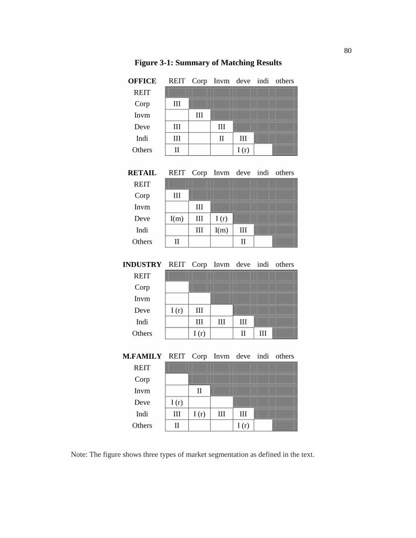
80
Figure 3-1: Summary of Matching Results
OFFICE REIT Corp Invm deve indi others
REIT
Corp III
Invm III
Deve III III
Indi III II III
Others II I (r)
RETAIL REIT Corp Invm deve indi others
REIT
Corp III
Invm III
Deve I(m) III I (r)
Indi III I(m) III
Others II II
INDUSTRY REIT Corp Invm deve indi others
REIT
Corp
Invm
Deve I (r) III
Indi III III III
Others I (r)
II III
M.FAMILY REIT Corp Invm deve indi others
REIT
Corp
Invm II
Deve I (r)
Indi III I (r) III III
Others II I (r)
Note: The figure shows three types of market segmentation as defined in the text.
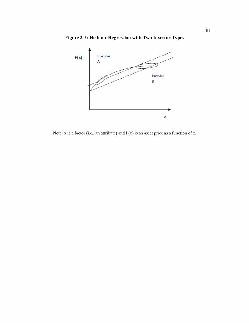
81
Figure 3-2: Hedonic Regression with Two Investor Types
Note: x is a factor (i.e., an attribute) and P(x) is an asset price as a function of x.
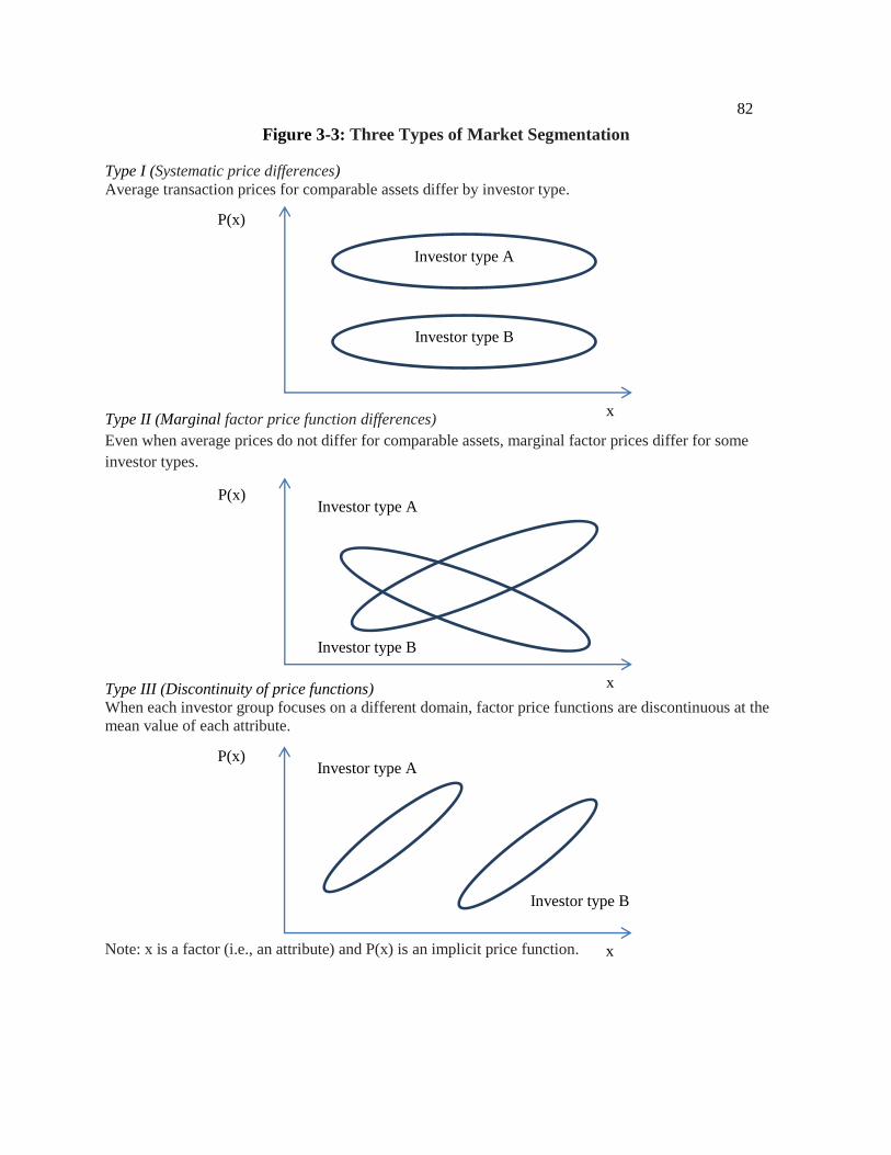
82
Figure 3-3: Three Types of Market Segmentation
Type I (Systematic price differences)
Average transaction prices for comparable assets differ by investor type.
Type II (Marginal factor price function differences)
Even when average prices do not differ for comparable assets, marginal factor prices differ for some
investor types.
Type III (Discontinuity of price functions)
When each investor group focuses on a different domain, factor price functions are discontinuous at the
mean value of each attribute.
Note: x is a factor (i.e., an attribute) and P(x) is an implicit price function.
x
P(x)
Investor type A
Investor type B
P(x)
Investor type A
Investor type B
x
P(x) Investor type A
x
Investor type B
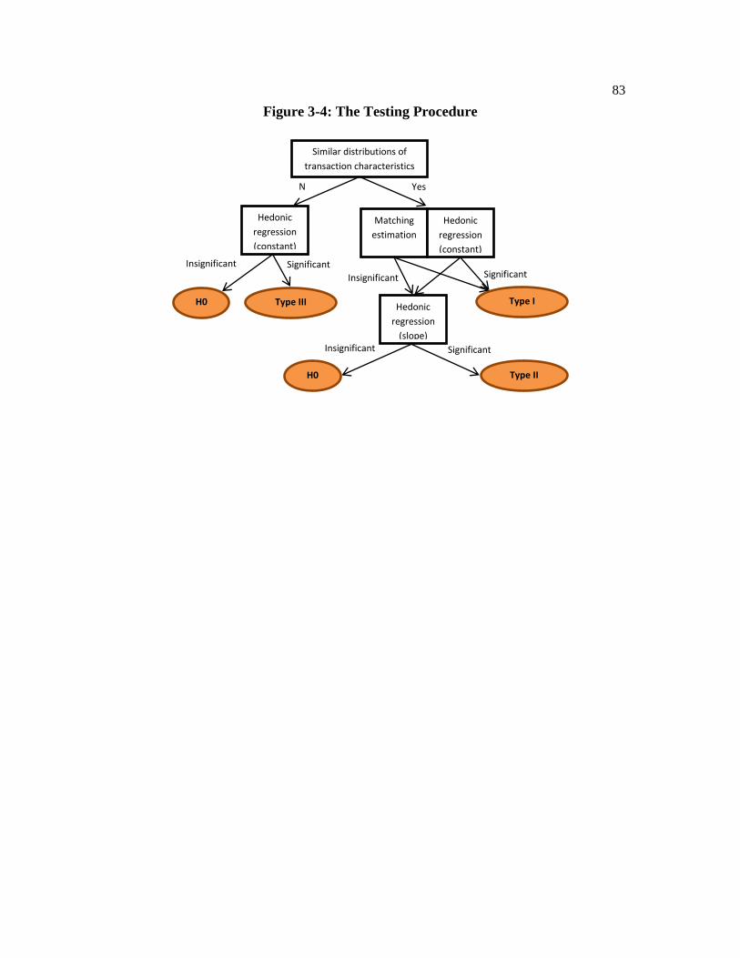
83
Figure 3-4: The Testing Procedure
Similar distributions of
transaction characteristics
Yes N
o
Matching
estimation
Insignificant
Type I
Hedonic
regression
(constant)
Significant
Hedonic
regression
(slope) Insignificant Significant
Type II
Hedonic
regression
(constant)
Insignificant Significant
Type III H0
H0
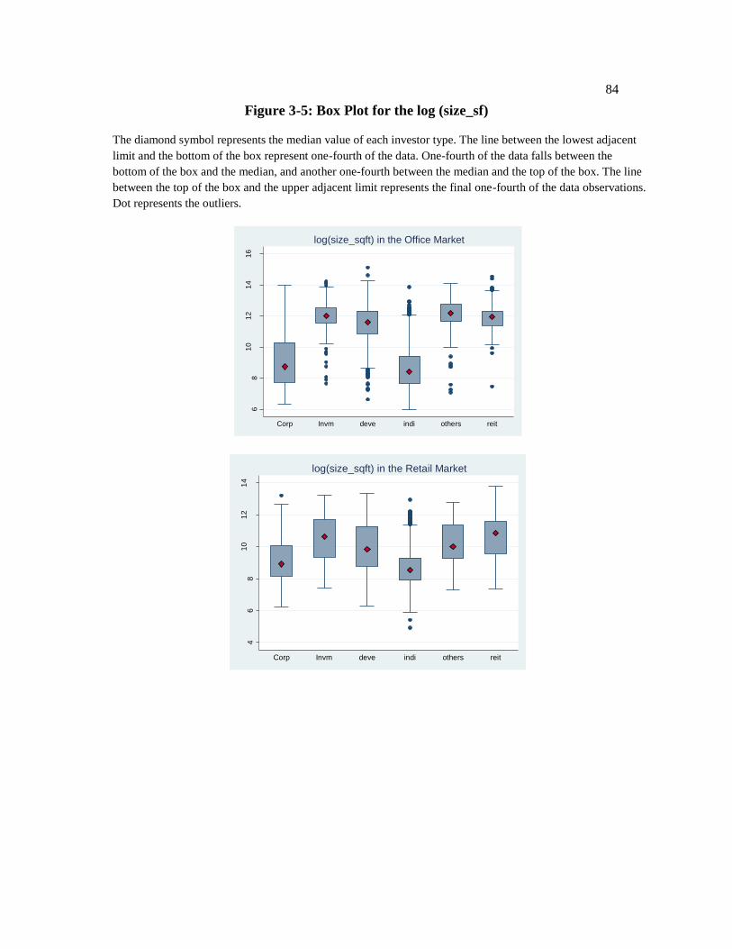
84
Figure 3-5: Box Plot for the log (size_sf)
The diamond symbol represents the median value of each investor type. The line between the lowest adjacent
limit and the bottom of the box represent one-fourth of the data. One-fourth of the data falls between the
bottom of the box and the median, and another one-fourth between the median and the top of the box. The line
between the top of the box and the upper adjacent limit represents the final one-fourth of the data observations.
Dot represents the outliers.
68
10
12
14
16
lnsiz
e
Corp Invm deve indi others reit
log(size_sqft) in the Office Market4
68
10
12
14
lnsiz
e
Corp Invm deve indi others reit
log(size_sqft) in the Retail Market
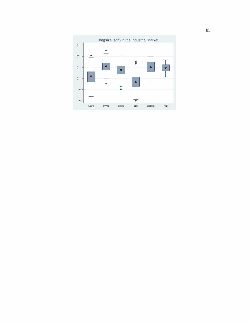
85
68
10
12
14
16
lnsiz
e
Corp Invm deve indi others reit
log(size_sqft) in the Industrial Market
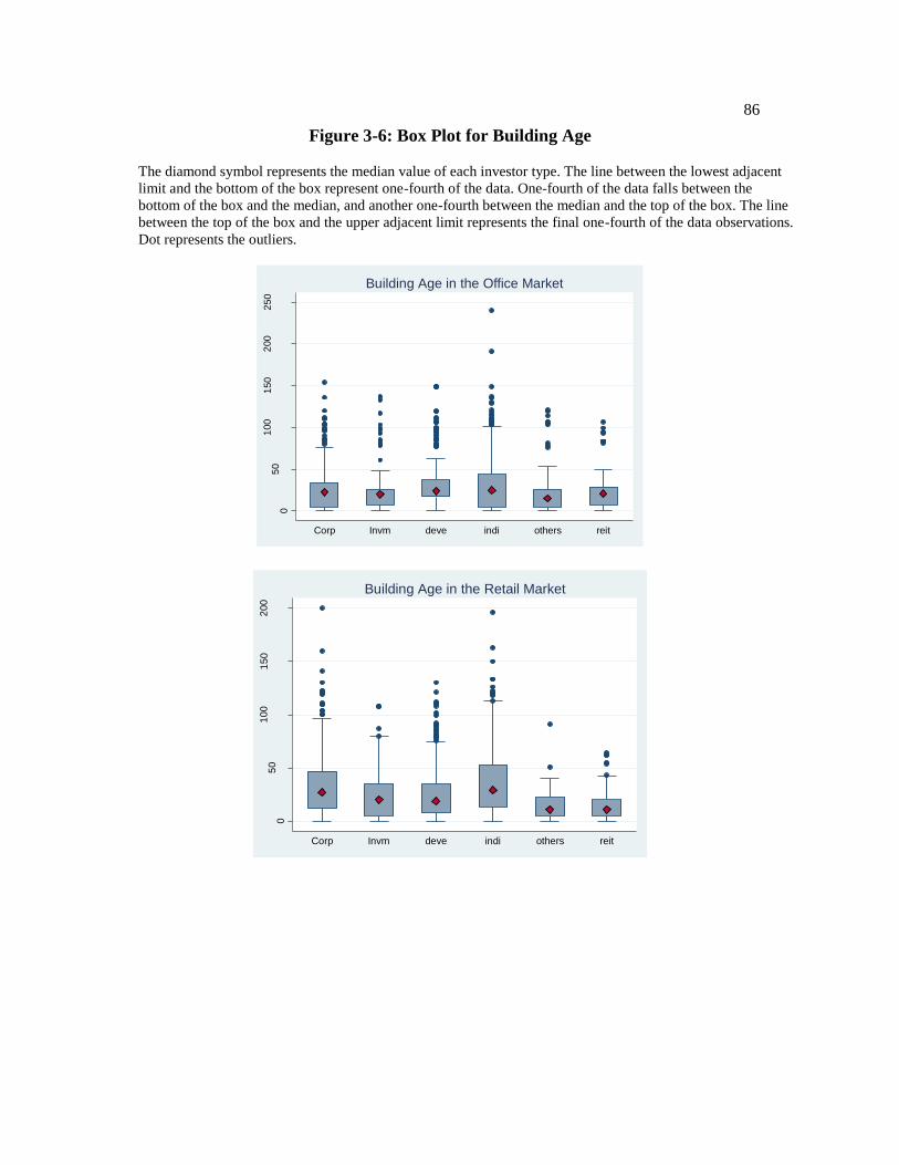
86
Figure 3-6: Box Plot for Building Age
The diamond symbol represents the median value of each investor type. The line between the lowest adjacent
limit and the bottom of the box represent one-fourth of the data. One-fourth of the data falls between the
bottom of the box and the median, and another one-fourth between the median and the top of the box. The line
between the top of the box and the upper adjacent limit represents the final one-fourth of the data observations.
Dot represents the outliers.
05
01
00
150
200
250
bda
ge
Corp Invm deve indi others reit
Building Age in the Office Market0
50
100
150
200
bda
ge
Corp Invm deve indi others reit
Building Age in the Retail Market
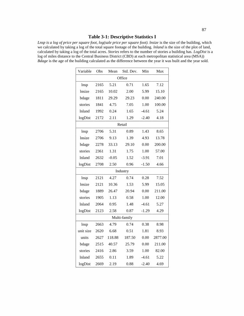
87
Table 3-1: Descriptive Statistics I
Lnsp is a log of price per square foot, log(sale price per square foot). lnsize is the size of the building, which
we calculated by taking a log of the total square footage of the building. lnland is the size of the plot of land,
calculated by taking a log of the total acres. Stories refers to the number of stories a building has. LogDist is a
log of miles distance to the Central Business District (CBD) at each metropolitan statistical area (MSA))
Bdage is the age of the building calculated as the difference between the year it was built and the year sold.
Variable Obs Mean Std. Dev. Min Max
Office
lnsp 2165 5.21 0.71 1.65 7.12
lnsize 2165 10.02 2.00 5.99 15.10
bdage 1811 29.29 29.23 0.00 240.00
stories 1841 4.75 7.05 1.00 100.00
lnland 1992 0.24 1.65 -4.61 5.24
logDist 2172 2.11 1.29 -2.40 4.18
Retail
lnsp 2706 5.31 0.89 1.43 8.65
lnsize 2706 9.13 1.39 4.93 13.78
bdage 2278 33.13 29.10 0.00 200.00
stories 2361 1.31 1.75 1.00 57.00
lnland 2632 -0.05 1.52 -3.91 7.01
logDist 2708 2.50 0.96 -1.50 4.66
Industry
lnsp 2121 4.27 0.74 0.28 7.52
lnsize 2121 10.36 1.53 5.99 15.05
bdage 1889 26.47 20.94 0.00 211.00
stories 1905 1.13 0.58 1.00 12.00
lnland 2064 0.95 1.48 -4.61 5.27
logDist 2123 2.58 0.87 -1.29 4.29
Multi-family
lnsp 2663 4.79 0.74 0.38 8.98
unit size 2620 6.68 0.51 1.81 8.93
units 2627 118.88 187.50 0.00 2877.00
bdage 2515 40.57 25.79 0.00 211.00
stories 2416 2.86 3.59 1.00 82.00
lnland 2655 0.11 1.89 -4.61 5.22
logDist 2669 2.19 0.88 -2.40 4.69
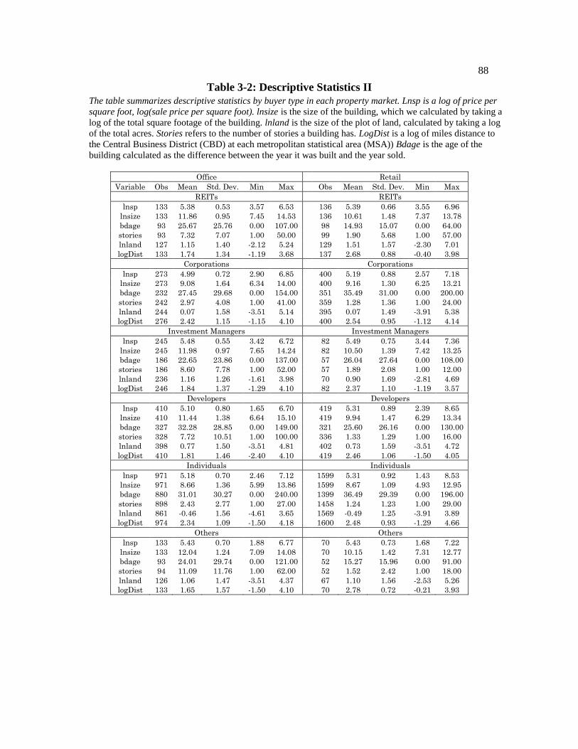
88
Table 3-2: Descriptive Statistics II
The table summarizes descriptive statistics by buyer type in each property market. Lnsp is a log of price per
square foot, log(sale price per square foot). lnsize is the size of the building, which we calculated by taking a
log of the total square footage of the building. lnland is the size of the plot of land, calculated by taking a log
of the total acres. Stories refers to the number of stories a building has. LogDist is a log of miles distance to
the Central Business District (CBD) at each metropolitan statistical area (MSA)) Bdage is the age of the
building calculated as the difference between the year it was built and the year sold.
Office Retail
Variable Obs Mean Std. Dev. Min Max Obs Mean Std. Dev. Min Max
REITs REITs
lnsp 133 5.38 0.53 3.57 6.53 136 5.39 0.66 3.55 6.96
lnsize 133 11.86 0.95 7.45 14.53 136 10.61 1.48 7.37 13.78
bdage 93 25.67 25.76 0.00 107.00 98 14.93 15.07 0.00 64.00
stories 93 7.32 7.07 1.00 50.00 99 1.90 5.68 1.00 57.00
lnland 127 1.15 1.40 -2.12 5.24 129 1.51 1.57 -2.30 7.01
logDist 133 1.74 1.34 -1.19 3.68 137 2.68 0.88 -0.40 3.98
Corporations Corporations
lnsp 273 4.99 0.72 2.90 6.85 400 5.19 0.88 2.57 7.18
lnsize 273 9.08 1.64 6.34 14.00 400 9.16 1.30 6.25 13.21
bdage 232 27.45 29.68 0.00 154.00 351 35.49 31.00 0.00 200.00
stories 242 2.97 4.08 1.00 41.00 359 1.28 1.36 1.00 24.00
lnland 244 0.07 1.58 -3.51 5.14 395 0.07 1.49 -3.91 5.38
logDist 276 2.42 1.15 -1.15 4.10 400 2.54 0.95 -1.12 4.14
Investment Managers Investment Managers
lnsp 245 5.48 0.55 3.42 6.72 82 5.49 0.75 3.44 7.36
lnsize 245 11.98 0.97 7.65 14.24 82 10.50 1.39 7.42 13.25
bdage 186 22.65 23.86 0.00 137.00 57 26.04 27.64 0.00 108.00
stories 186 8.60 7.78 1.00 52.00 57 1.89 2.08 1.00 12.00
lnland 236 1.16 1.26 -1.61 3.98 70 0.90 1.69 -2.81 4.69
logDist 246 1.84 1.37 -1.29 4.10 82 2.37 1.10 -1.19 3.57
Developers Developers
lnsp 410 5.10 0.80 1.65 6.70 419 5.31 0.89 2.39 8.65
lnsize 410 11.44 1.38 6.64 15.10 419 9.94 1.47 6.29 13.34
bdage 327 32.28 28.85 0.00 149.00 321 25.60 26.16 0.00 130.00
stories 328 7.72 10.51 1.00 100.00 336 1.33 1.29 1.00 16.00
lnland 398 0.77 1.50 -3.51 4.81 402 0.73 1.59 -3.51 4.72
logDist 410 1.81 1.46 -2.40 4.10 419 2.46 1.06 -1.50 4.05
Individuals Individuals
lnsp 971 5.18 0.70 2.46 7.12 1599 5.31 0.92 1.43 8.53
lnsize 971 8.66 1.36 5.99 13.86 1599 8.67 1.09 4.93 12.95
bdage 880 31.01 30.27 0.00 240.00 1399 36.49 29.39 0.00 196.00
stories 898 2.43 2.77 1.00 27.00 1458 1.24 1.23 1.00 29.00
lnland 861 -0.46 1.56 -4.61 3.65 1569 -0.49 1.25 -3.91 3.89
logDist 974 2.34 1.09 -1.50 4.18 1600 2.48 0.93 -1.29 4.66
Others Others
lnsp 133 5.43 0.70 1.88 6.77 70 5.43 0.73 1.68 7.22
lnsize 133 12.04 1.24 7.09 14.08 70 10.15 1.42 7.31 12.77
bdage 93 24.01 29.74 0.00 121.00 52 15.27 15.96 0.00 91.00
stories 94 11.09 11.76 1.00 62.00 52 1.52 2.42 1.00 18.00
lnland 126 1.06 1.47 -3.51 4.37 67 1.10 1.56 -2.53 5.26
logDist 133 1.65 1.57 -1.50 4.10 70 2.78 0.72 -0.21 3.93
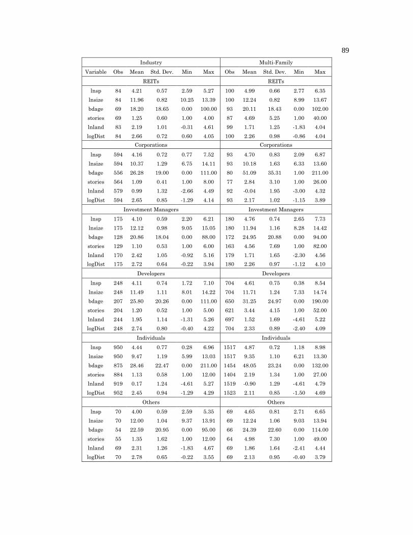
89
Industry Multi-Family
Variable Obs Mean Std. Dev. Min Max Obs Mean Std. Dev. Min Max
REITs REITs
lnsp 84 4.21 0.57 2.59 5.27 100 4.99 0.66 2.77 6.35
lnsize 84 11.96 0.82 10.25 13.39 100 12.24 0.82 8.99 13.67
bdage 69 18.20 18.65 0.00 100.00 93 20.11 18.43 0.00 102.00
stories 69 1.25 0.60 1.00 4.00 87 4.69 5.25 1.00 40.00
lnland 83 2.19 1.01 -0.31 4.61 99 1.71 1.25 -1.83 4.04
logDist 84 2.66 0.72 0.60 4.05 100 2.26 0.98 -0.86 4.04
Corporations Corporations
lnsp 594 4.16 0.72 0.77 7.52 93 4.70 0.83 2.09 6.87
lnsize 594 10.37 1.29 6.75 14.11 93 10.18 1.63 6.33 13.60
bdage 556 26.28 19.00 0.00 111.00 80 51.09 35.31 1.00 211.00
stories 564 1.09 0.41 1.00 8.00 77 2.84 3.10 1.00 26.00
lnland 579 0.99 1.32 -2.66 4.49 92 -0.04 1.95 -3.00 4.32
logDist 594 2.65 0.85 -1.29 4.14 93 2.17 1.02 -1.15 3.89
Investment Managers Investment Managers
lnsp 175 4.10 0.59 2.20 6.21 180 4.76 0.74 2.65 7.73
lnsize 175 12.12 0.98 9.05 15.05 180 11.94 1.16 8.28 14.42
bdage 128 20.86 18.04 0.00 88.00 172 24.95 20.88 0.00 94.00
stories 129 1.10 0.53 1.00 6.00 163 4.56 7.69 1.00 82.00
lnland 170 2.42 1.05 -0.92 5.16 179 1.71 1.65 -2.30 4.56
logDist 175 2.72 0.64 -0.22 3.94 180 2.26 0.97 -1.12 4.10
Developers Developers
lnsp 248 4.11 0.74 1.72 7.10 704 4.61 0.75 0.38 8.54
lnsize 248 11.49 1.11 8.01 14.22 704 11.71 1.24 7.33 14.74
bdage 207 25.80 20.26 0.00 111.00 650 31.25 24.97 0.00 190.00
stories 204 1.20 0.52 1.00 5.00 621 3.44 4.15 1.00 52.00
lnland 244 1.95 1.14 -1.31 5.26 697 1.52 1.69 -4.61 5.22
logDist 248 2.74 0.80 -0.40 4.22 704 2.33 0.89 -2.40 4.09
Individuals Individuals
lnsp 950 4.44 0.77 0.28 6.96 1517 4.87 0.72 1.18 8.98
lnsize 950 9.47 1.19 5.99 13.03 1517 9.35 1.10 6.21 13.30
bdage 875 28.46 22.47 0.00 211.00 1454 48.05 23.24 0.00 132.00
stories 884 1.13 0.58 1.00 12.00 1404 2.19 1.34 1.00 27.00
lnland 919 0.17 1.24 -4.61 5.27 1519 -0.90 1.29 -4.61 4.79
logDist 952 2.45 0.94 -1.29 4.29 1523 2.11 0.85 -1.50 4.69
Others Others
lnsp 70 4.00 0.59 2.59 5.35 69 4.65 0.81 2.71 6.65
lnsize 70 12.00 1.04 9.37 13.91 69 12.24 1.06 9.03 13.94
bdage 54 22.59 20.95 0.00 95.00 66 24.39 22.60 0.00 114.00
stories 55 1.35 1.62 1.00 12.00 64 4.98 7.30 1.00 49.00
lnland 69 2.31 1.26 -1.83 4.67 69 1.86 1.64 -2.41 4.44
logDist 70 2.78 0.65 -0.22 3.55 69 2.13 0.95 -0.40 3.79

90
Table 3-3: Description and Definition of Investor Type Investor type Costar’s description Examples Definition
REIT Traded on a public market,
must have REIT type tax
status
Prologis
Liberty Property
Trust,
SimonProperty
Group, Inc.
A real estate investment trust, or REIT, is a
company that owns, and in most cases, operates
income-producing real estate. Some REITs also
engage in financing real estate. The shares of
many REITs are traded on major stock
exchanges.
Corporate Corporate user or retailer or
business or company user
Adobe Systems
Inc
A company that purchases real estate to operate
a business. The corporation can be a small
private manufacturer or a large publically traded
company.
Investment
managers
Investment manager or
advisor
RREFF
AEW Capital
Management
This group provides real estate investment
strategy and operating knowledge to various
groups of equity institutional investors.
Investment managers operate separate accounts,
sponsor funds and other real estate investment
programs as well as develop and manage the
assets in which they invest. They serve the
investment goals of public and corporate
pension funds, foundations, endowments,
insurance companies and individuals.
developers Non-traded privately held
development/property
manager/owner/operator that
owns properties
Adler Realty
Investments Inc
A private real estate company owner that can
also develop, manage and operate its assets. The
company buys and sells properties.
individuals Individual or a small group of
individual investor
Chawla
Properties, LLC
Individual or small group of individuals that
invest directly and own real estate property.
others Pension Fund
Insurance
Equity fund
Private REIT
Prudential
Insurance Group
Federal Capital
Partners
Equity fund established by an employer to
facilitate and organize the investment of
employees' retirement funds contributed by the
employer and employees. The pension fund is a
common asset pool meant to generate stable
growth over the long term, and provide pensions
for employees when they reach the end of their
working years and commence retirement.
A public or private insurance company
purchases real estate for income or increase
return of capital upon sale. The purchases are
not user intended as a location to operate a
business.
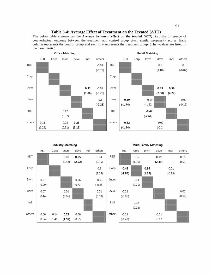
91
Table 3-4: Average Effect of Treatment on the Treated (ATT) The below table summarizes the Average treatment effect on the treated (ATT), i.e., the difference of
counterfactual outcome between the treatment and control group given similar propensity scores. Each
column represents the control group and each row represents the treatment group. (The t-values are listed in
the parenthesis.)
Office Matching Retail Matching
REIT Corp Invm deve indi others
REIT Corp Invm deve indi others
REIT -0.08
(-0.78)
REIT 0.1
(1.18)
0
(-0.02)
Corp Corp
Invm 0.31
(1.86)
-0.02
(-0.28)
Invm 0.33
(2.58)
0.59
(4.27)
deve -0.3
(-2.28)
deve -0.19
(-1.74)
-0.19
(-1.22)
-0.02
(-0.15)
indi 0.17
(0.37)
indi -0.42
(-2.64)
others 0.11
(1.22)
0.03
(0.31)
0.25
(3.13)
others -0.32
(-1.94)
-0.02
(-0.1)
Industry Matching Multi-Family Matching
REIT Corp Invm deve indi others
REIT Corp Invm deve indi others
REIT 0.08
(0.48)
0.25
(2.52)
0.04
(0.35)
REIT 0.36
(1.36)
0.19
(2.39)
0.16
(0.51)
Corp 0.2
(1.08)
Corp -0.48
(-1.89)
0.86
(1.69)
-0.01
(-0.13)
Invm 0.01
(0.09)
0.06
(0.73)
-0.03
(-0.25)
Invm 0.13
(0.75)
deve 0.07
(0.44)
0.01
(0.06)
0.01
(0.09)
deve -0.11
(-0.86)
0.07
(0.59)
indi indi 0.02
(0.18)
others 0.06
(0.54)
0.14
(1.41)
0.22
(1.92)
0.06
(0.55)
others -0.21
(-1.49)
-0.01
-0.12
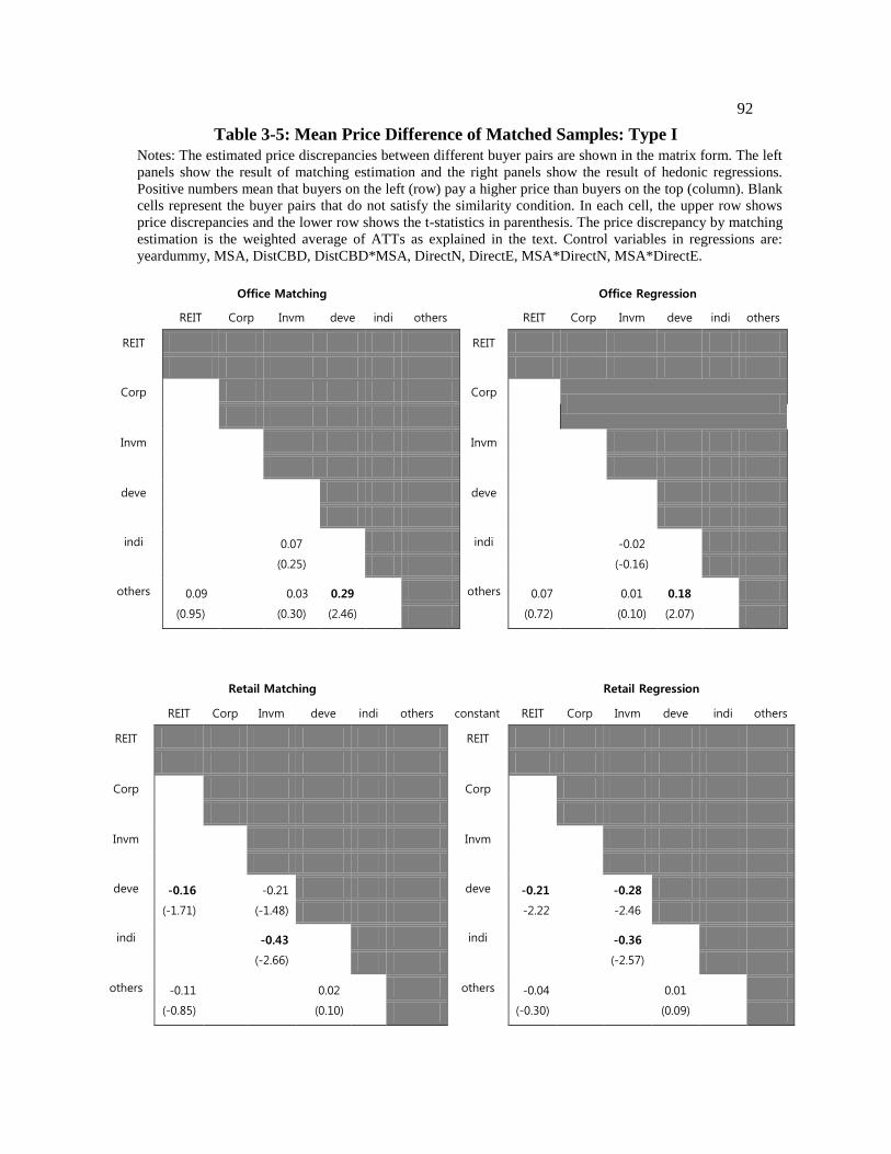
92
Table 3-5: Mean Price Difference of Matched Samples: Type I
Notes: The estimated price discrepancies between different buyer pairs are shown in the matrix form. The left
panels show the result of matching estimation and the right panels show the result of hedonic regressions.
Positive numbers mean that buyers on the left (row) pay a higher price than buyers on the top (column). Blank
cells represent the buyer pairs that do not satisfy the similarity condition. In each cell, the upper row shows
price discrepancies and the lower row shows the t-statistics in parenthesis. The price discrepancy by matching
estimation is the weighted average of ATTs as explained in the text. Control variables in regressions are:
yeardummy, MSA, DistCBD, DistCBD*MSA, DirectN, DirectE, MSA*DirectN, MSA*DirectE.
Office Matching
Office Regression
REIT Corp Invm deve indi others
REIT Corp Invm deve indi others
REIT REIT
Corp
Corp
Invm
Invm
deve deve
indi
0.07
(0.25)
indi
-0.02
(-0.16)
others 0.09
(0.95)
0.03
(0.30)
0.29
(2.46)
others 0.07
(0.72)
0.01
(0.10)
0.18
(2.07)
Retail Matching
Retail Regression
REIT Corp Invm deve indi others constant REIT Corp Invm deve indi others
REIT REIT
Corp Corp
Invm Invm
deve -0.16
(-1.71)
-0.21
(-1.48)
deve -0.21
-2.22
-0.28
-2.46
indi -0.43
(-2.66)
indi
-0.36
(-2.57)
others -0.11
(-0.85)
0.02
(0.10)
others -0.04
(-0.30)
0.01
(0.09)
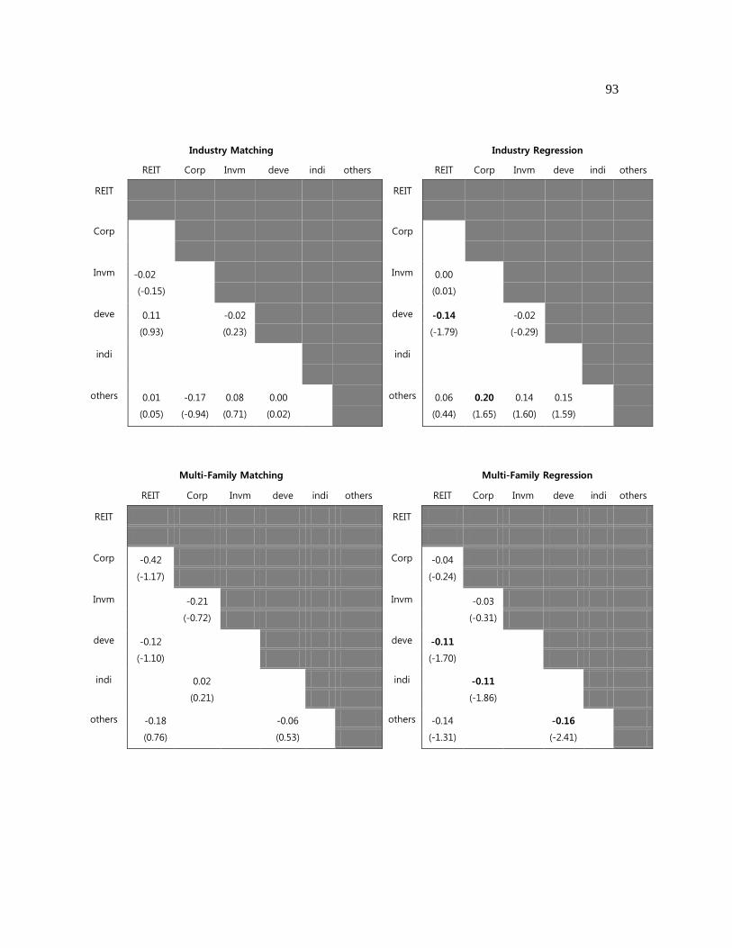
93
Industry Matching
Industry Regression
REIT Corp Invm deve indi others
REIT Corp Invm deve indi others
REIT
REIT
Corp
Corp
Invm -0.02
(-0.15)
Invm 0.00
(0.01)
deve 0.11
(0.93)
-0.02
(0.23)
deve -0.14
(-1.79)
-0.02
(-0.29)
indi
indi
others 0.01
(0.05)
-0.17
(-0.94)
0.08
(0.71)
0.00
(0.02)
others 0.06
(0.44)
0.20
(1.65)
0.14
(1.60)
0.15
(1.59)
Multi-Family Matching Multi-Family Regression
REIT Corp Invm deve indi others
REIT Corp Invm deve indi others
REIT REIT
Corp -0.42
(-1.17)
Corp -0.04
(-0.24)
Invm -0.21
(-0.72)
Invm -0.03
(-0.31)
deve -0.12
(-1.10)
deve -0.11
(-1.70)
indi 0.02
(0.21)
indi
-0.11
(-1.86)
others -0.18
(0.76)
-0.06
(0.53)
others -0.14
(-1.31)
-0.16
(-2.41)
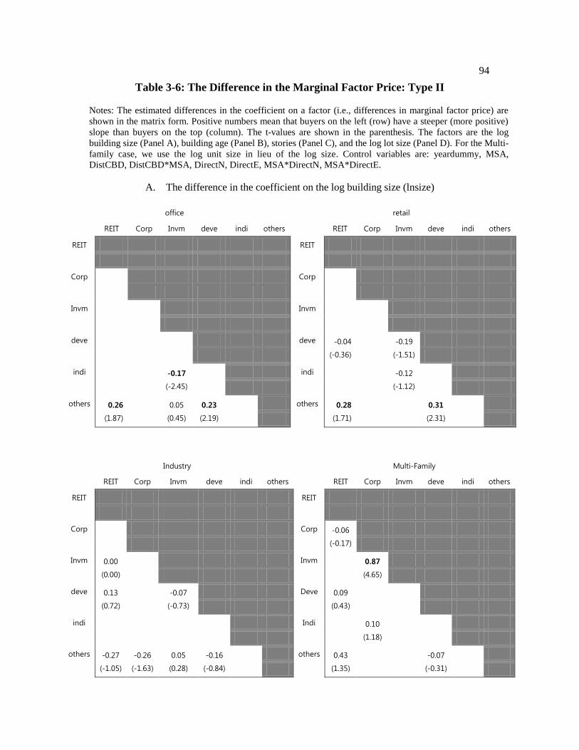
94
Table 3-6: The Difference in the Marginal Factor Price: Type II
Notes: The estimated differences in the coefficient on a factor (i.e., differences in marginal factor price) are
shown in the matrix form. Positive numbers mean that buyers on the left (row) have a steeper (more positive)
slope than buyers on the top (column). The t-values are shown in the parenthesis. The factors are the log
building size (Panel A), building age (Panel B), stories (Panel C), and the log lot size (Panel D). For the Multi-
family case, we use the log unit size in lieu of the log size. Control variables are: yeardummy, MSA,
DistCBD, DistCBD*MSA, DirectN, DirectE, MSA*DirectN, MSA*DirectE.
A. The difference in the coefficient on the log building size (lnsize)
office
retail
REIT Corp Invm deve indi others
REIT Corp Invm deve indi others
REIT REIT
Corp
Corp
Invm
Invm
deve
deve -0.04
(-0.36)
-0.19
(-1.51)
indi
-0.17
(-2.45)
indi
-0.12
(-1.12)
others 0.26
(1.87)
0.05
(0.45)
0.23
(2.19)
others 0.28
(1.71)
0.31
(2.31)
Industry
Multi-Family
REIT Corp Invm deve indi others
REIT Corp Invm deve indi others
REIT REIT
Corp
Corp -0.06
(-0.17)
Invm 0.00
(0.00)
Invm
0.87
(4.65)
deve 0.13
(0.72)
-0.07
(-0.73)
Deve 0.09
(0.43)
indi
Indi
0.10
(1.18)
others -0.27
(-1.05)
-0.26
(-1.63)
0.05
(0.28)
-0.16
(-0.84)
others 0.43
(1.35)
-0.07
(-0.31)
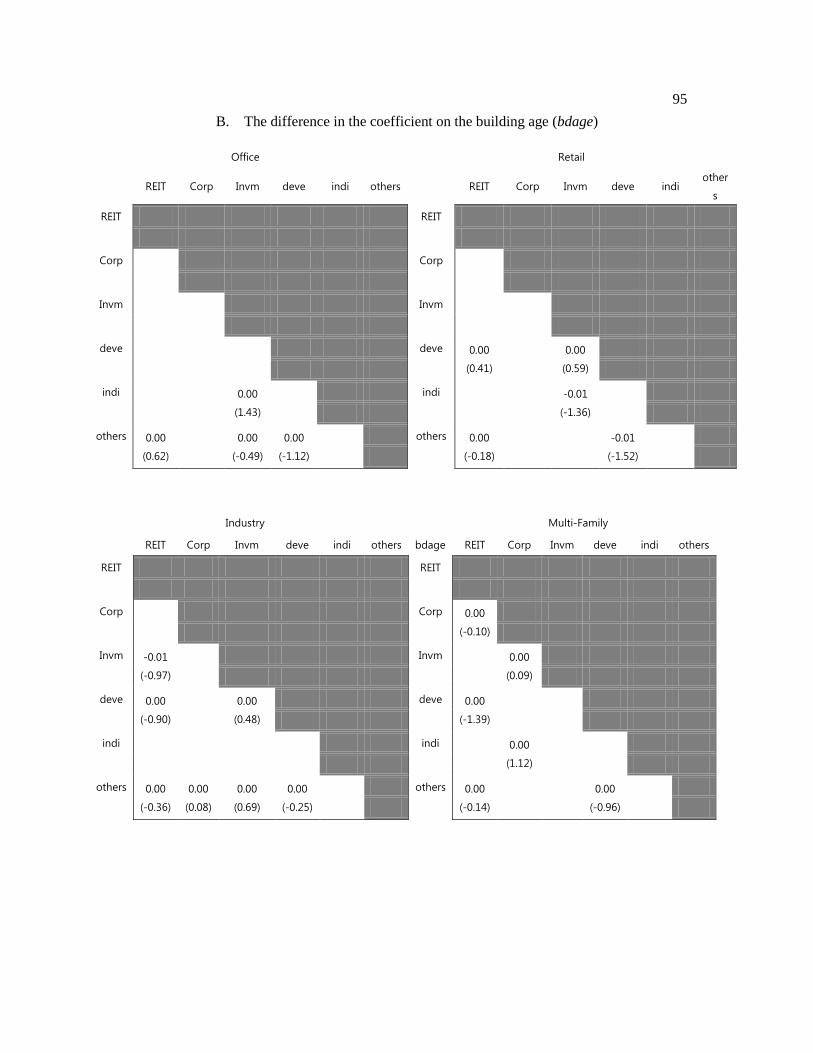
95
B. The difference in the coefficient on the building age (bdage)
Office
Retail
REIT Corp Invm deve indi others
REIT Corp Invm deve indi
other
s
REIT REIT
Corp
Corp
Invm
Invm
deve
deve 0.00
(0.41)
0.00
(0.59)
indi
0.00
(1.43)
indi
-0.01
(-1.36)
others 0.00
(0.62)
0.00
(-0.49)
0.00
(-1.12)
others 0.00
(-0.18)
-0.01
(-1.52)
Industry
Multi-Family
REIT Corp Invm deve indi others bdage REIT Corp Invm deve indi others
REIT REIT
Corp
Corp 0.00
(-0.10)
Invm -0.01
(-0.97)
Invm
0.00
(0.09)
deve 0.00
(-0.90)
0.00
(0.48)
deve 0.00
(-1.39)
indi
indi
0.00
(1.12)
others 0.00
(-0.36)
0.00
(0.08)
0.00
(0.69)
0.00
(-0.25)
others 0.00
(-0.14)
0.00
(-0.96)
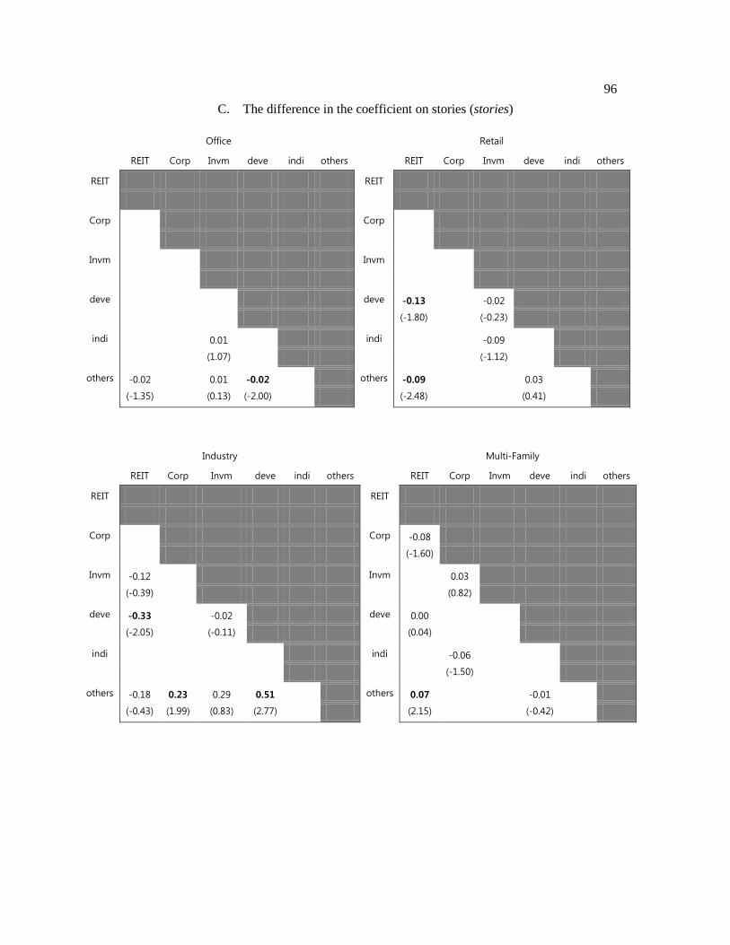
96
C. The difference in the coefficient on stories (stories)
Office
Retail
REIT Corp Invm deve indi others
REIT Corp Invm deve indi others
REIT REIT
Corp
Corp
Invm
Invm
deve
deve -0.13
(-1.80)
-0.02
(-0.23)
indi
0.01
(1.07)
indi
-0.09
(-1.12)
others -0.02
(-1.35)
0.01
(0.13)
-0.02
(-2.00)
others -0.09
(-2.48)
0.03
(0.41)
Industry
Multi-Family
REIT Corp Invm deve indi others
REIT Corp Invm deve indi others
REIT REIT
Corp
Corp -0.08
(-1.60)
Invm -0.12
(-0.39)
Invm
0.03
(0.82)
deve -0.33
(-2.05)
-0.02
(-0.11)
deve 0.00
(0.04)
indi
indi
-0.06
(-1.50)
others -0.18
(-0.43)
0.23
(1.99)
0.29
(0.83)
0.51
(2.77)
others 0.07
(2.15)
-0.01
(-0.42)

97
D. The difference in the coefficient on the log lot size (lnland)
Office
Retail
REIT Corp Invm deve indi
other
s REIT Corp Invm deve indi others
REIT REIT
Corp
Corp
Invm
Invm
deve
deve -0.08
(-0.62)
0.15
(1.17)
indi
-0.01
(-0.13)
indi
0.00
(-0.03)
others -0.07
(-0.81)
0.03
(0.40)
0.02
(0.28)
others -0.33
(-1.79)
-0.18
(-1.20)
Industry
Multi-Family
REIT Corp Invm deve indi others
REIT Corp Invm deve indi others
REIT REIT
Corp
Corp -0.11
(-0.85)
Invm -0.03
(-0.19)
Invm
0.08
(1.14)
deve -0.29
(-1.72)
-0.12
(-1.36)
deve -0.10
(-1.58)
indi
indi
-0.05
(-0.80)
others 0.15
(0.59)
0.29
(1.93)
-0.08
(-0.46)
0.26
(1.37)
others 0.09
(0.77)
0.07
(1.18)
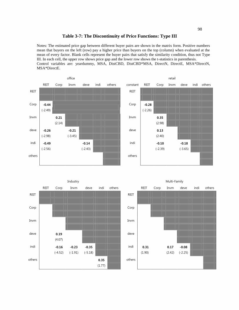
98
Table 3-7: The Discontinuity of Price Functions: Type III
Notes: The estimated price gap between different buyer pairs are shown in the matrix form. Positive numbers
mean that buyers on the left (row) pay a higher price than buyers on the top (column) when evaluated at the
mean of every factor. Blank cells represent the buyer pairs that satisfy the similarity condition, thus not Type
III. In each cell, the upper row shows price gap and the lower row shows the t-statistics in parenthesis.
Control variables are: yeardummy, MSA, DistCBD, DistCBD*MSA, DirectN, DirectE, MSA*DirectN,
MSA*DirectE.
office
retail
REIT Corp Invm deve indi others
constant REIT Corp Invm deve indi others
REIT
REIT
Corp -0.44
(-2.49)
Corp -0.28
(-2.26)
Invm
0.21
(2.14)
Invm
0.35
(2.98)
deve -0.26
(-2.98)
-0.21
(-3.45)
deve
0.13
(2.40)
indi -0.49
(-2.56)
-0.14
(-2.43)
indi
-0.10
(-2.39)
-0.18
(-3.65)
others
others
Industry
Multi-Family
REIT Corp Invm deve indi others
REIT Corp Invm deve indi others
REIT
REIT
Corp
Corp
Invm
Invm
deve
0.19
(4.07)
deve
indi
-0.16
(-4.52)
-0.23
(-1.91)
-0.35
(-5.18)
indi 0.31
(1.90)
0.17
(2.42)
-0.08
(-2.25)
others
0.35
(1.77)
others
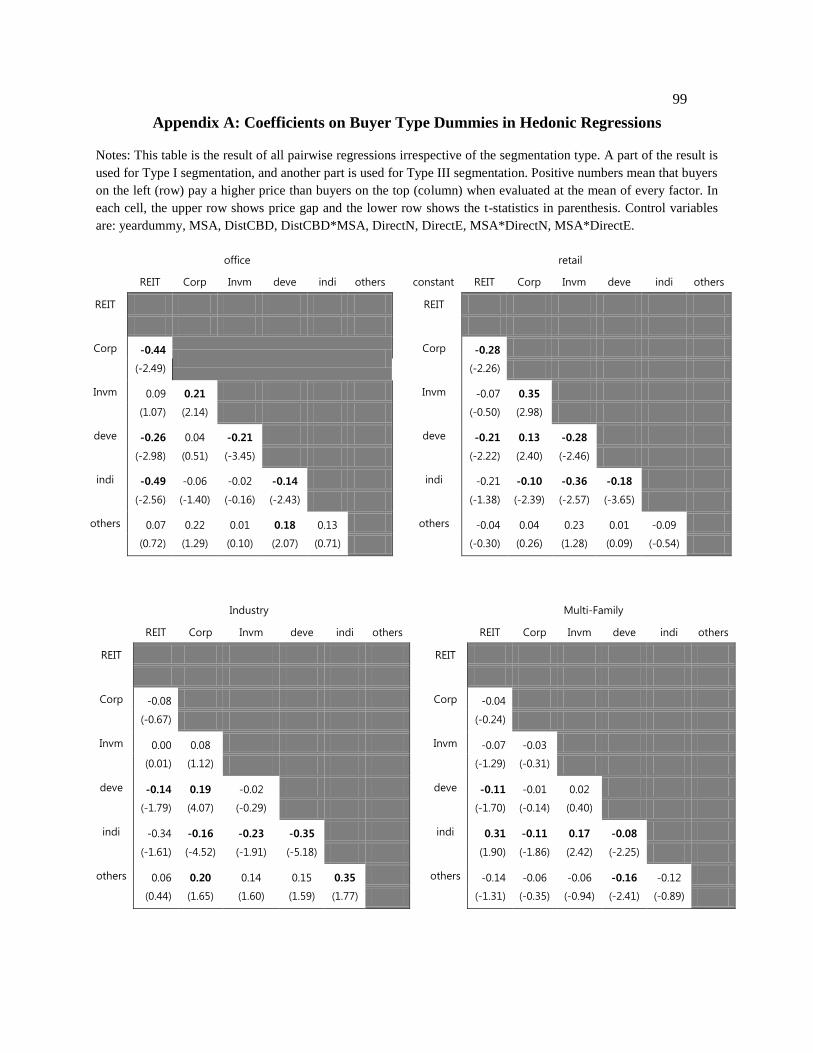
99
Appendix A: Coefficients on Buyer Type Dummies in Hedonic Regressions
Notes: This table is the result of all pairwise regressions irrespective of the segmentation type. A part of the result is
used for Type I segmentation, and another part is used for Type III segmentation. Positive numbers mean that buyers
on the left (row) pay a higher price than buyers on the top (column) when evaluated at the mean of every factor. In
each cell, the upper row shows price gap and the lower row shows the t-statistics in parenthesis. Control variables
are: yeardummy, MSA, DistCBD, DistCBD*MSA, DirectN, DirectE, MSA*DirectN, MSA*DirectE.
office
retail
REIT Corp Invm deve indi others
constant REIT Corp Invm deve indi others
REIT
REIT
Corp -0.44
(-2.49)
Corp -0.28
(-2.26)
Invm 0.09
(1.07)
0.21
(2.14)
Invm -0.07
(-0.50)
0.35
(2.98)
deve -0.26
(-2.98)
0.04
(0.51)
-0.21
(-3.45)
deve -0.21
(-2.22)
0.13
(2.40)
-0.28
(-2.46)
indi -0.49
(-2.56)
-0.06
(-1.40)
-0.02
(-0.16)
-0.14
(-2.43)
indi -0.21
(-1.38)
-0.10
(-2.39)
-0.36
(-2.57)
-0.18
(-3.65)
others 0.07
(0.72)
0.22
(1.29)
0.01
(0.10)
0.18
(2.07)
0.13
(0.71)
others -0.04
(-0.30)
0.04
(0.26)
0.23
(1.28)
0.01
(0.09)
-0.09
(-0.54)
Industry
Multi-Family
REIT Corp Invm deve indi others
REIT Corp Invm deve indi others
REIT
REIT
Corp -0.08
(-0.67)
Corp -0.04
(-0.24)
Invm 0.00
(0.01)
0.08
(1.12)
Invm -0.07
(-1.29)
-0.03
(-0.31)
deve -0.14
(-1.79)
0.19
(4.07)
-0.02
(-0.29)
deve -0.11
(-1.70)
-0.01
(-0.14)
0.02
(0.40)
indi -0.34
(-1.61)
-0.16
(-4.52)
-0.23
(-1.91)
-0.35
(-5.18)
indi 0.31
(1.90)
-0.11
(-1.86)
0.17
(2.42)
-0.08
(-2.25)
others 0.06
(0.44)
0.20
(1.65)
0.14
(1.60)
0.15
(1.59)
0.35
(1.77)
others -0.14
(-1.31)
-0.06
(-0.35)
-0.06
(-0.94)
-0.16
(-2.41)
-0.12
(-0.89)
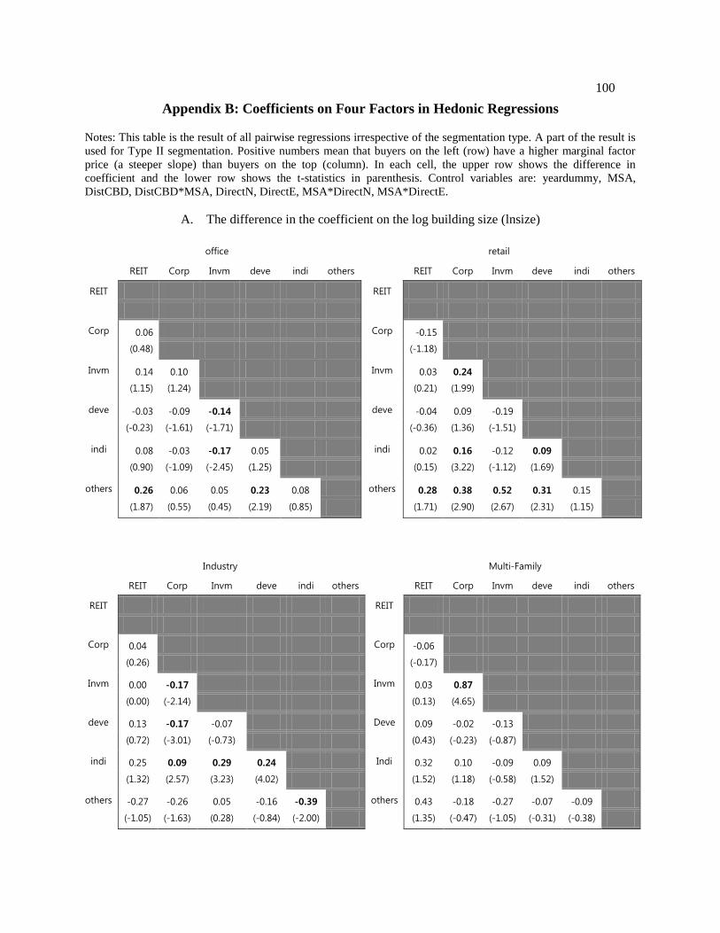
100
Appendix B: Coefficients on Four Factors in Hedonic Regressions
Notes: This table is the result of all pairwise regressions irrespective of the segmentation type. A part of the result is
used for Type II segmentation. Positive numbers mean that buyers on the left (row) have a higher marginal factor
price (a steeper slope) than buyers on the top (column). In each cell, the upper row shows the difference in
coefficient and the lower row shows the t-statistics in parenthesis. Control variables are: yeardummy, MSA,
DistCBD, DistCBD*MSA, DirectN, DirectE, MSA*DirectN, MSA*DirectE.
A. The difference in the coefficient on the log building size (lnsize)
office
retail
REIT Corp Invm deve indi others
REIT Corp Invm deve indi others
REIT REIT
Corp 0.06
(0.48)
Corp -0.15
(-1.18)
Invm 0.14
(1.15)
0.10
(1.24)
Invm 0.03
(0.21)
0.24
(1.99)
deve -0.03
(-0.23)
-0.09
(-1.61)
-0.14
(-1.71)
deve -0.04
(-0.36)
0.09
(1.36)
-0.19
(-1.51)
indi 0.08
(0.90)
-0.03
(-1.09)
-0.17
(-2.45)
0.05
(1.25)
indi 0.02
(0.15)
0.16
(3.22)
-0.12
(-1.12)
0.09
(1.69)
others 0.26
(1.87)
0.06
(0.55)
0.05
(0.45)
0.23
(2.19)
0.08
(0.85)
others 0.28
(1.71)
0.38
(2.90)
0.52
(2.67)
0.31
(2.31)
0.15
(1.15)
Industry
Multi-Family
REIT Corp Invm deve indi others
REIT Corp Invm deve indi others
REIT REIT
Corp 0.04
(0.26)
Corp -0.06
(-0.17)
Invm 0.00
(0.00)
-0.17
(-2.14)
Invm 0.03
(0.13)
0.87
(4.65)
deve 0.13
(0.72)
-0.17
(-3.01)
-0.07
(-0.73)
Deve 0.09
(0.43)
-0.02
(-0.23)
-0.13
(-0.87)
indi 0.25
(1.32)
0.09
(2.57)
0.29
(3.23)
0.24
(4.02)
Indi 0.32
(1.52)
0.10
(1.18)
-0.09
(-0.58)
0.09
(1.52)
others -0.27
(-1.05)
-0.26
(-1.63)
0.05
(0.28)
-0.16
(-0.84)
-0.39
(-2.00)
others 0.43
(1.35)
-0.18
(-0.47)
-0.27
(-1.05)
-0.07
(-0.31)
-0.09
(-0.38)
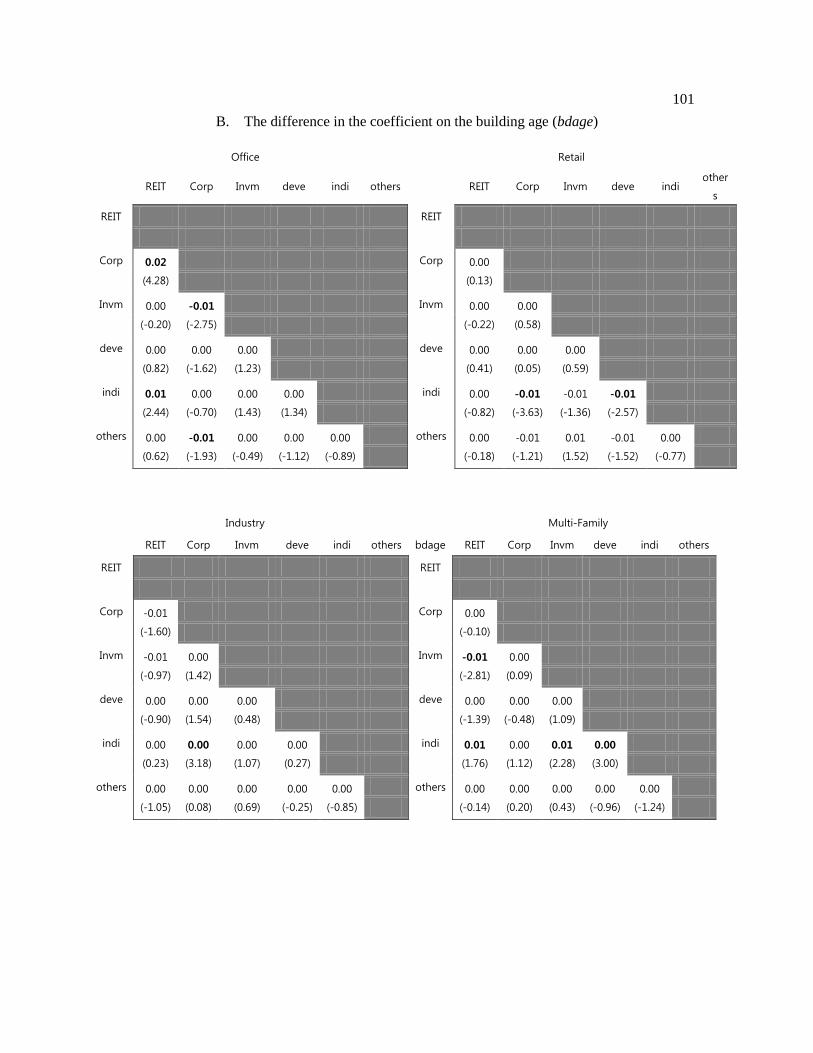
101
B. The difference in the coefficient on the building age (bdage)
Office
Retail
REIT Corp Invm deve indi others
REIT Corp Invm deve indi
other
s
REIT REIT
Corp 0.02
(4.28)
Corp 0.00
(0.13)
Invm 0.00
(-0.20)
-0.01
(-2.75)
Invm 0.00
(-0.22)
0.00
(0.58)
deve 0.00
(0.82)
0.00
(-1.62)
0.00
(1.23)
deve 0.00
(0.41)
0.00
(0.05)
0.00
(0.59)
indi 0.01
(2.44)
0.00
(-0.70)
0.00
(1.43)
0.00
(1.34)
indi 0.00
(-0.82)
-0.01
(-3.63)
-0.01
(-1.36)
-0.01
(-2.57)
others 0.00
(0.62)
-0.01
(-1.93)
0.00
(-0.49)
0.00
(-1.12)
0.00
(-0.89)
others 0.00
(-0.18)
-0.01
(-1.21)
0.01
(1.52)
-0.01
(-1.52)
0.00
(-0.77)
Industry
Multi-Family
REIT Corp Invm deve indi others bdage REIT Corp Invm deve indi others
REIT REIT
Corp -0.01
(-1.60)
Corp 0.00
(-0.10)
Invm -0.01
(-0.97)
0.00
(1.42)
Invm -0.01
(-2.81)
0.00
(0.09)
deve 0.00
(-0.90)
0.00
(1.54)
0.00
(0.48)
deve 0.00
(-1.39)
0.00
(-0.48)
0.00
(1.09)
indi 0.00
(0.23)
0.00
(3.18)
0.00
(1.07)
0.00
(0.27)
indi 0.01
(1.76)
0.00
(1.12)
0.01
(2.28)
0.00
(3.00)
others 0.00
(-1.05)
0.00
(0.08)
0.00
(0.69)
0.00
(-0.25)
0.00
(-0.85)
others 0.00
(-0.14)
0.00
(0.20)
0.00
(0.43)
0.00
(-0.96)
0.00
(-1.24)

102
C. The difference in the coefficient on stories (stories)
Office
Retail
REIT Corp Invm deve indi others
REIT Corp Invm deve indi others
REIT REIT
Corp -0.02
(-0.81)
Corp 0.00
(-0.08)
Invm -0.01
(-0.82)
-0.01
(-0.64)
Invm 0.04
(0.56)
-0.07
(-1.03)
deve 0.00
(0.29)
0.00
(0.31)
0.02
(2.08)
deve -0.13
(-1.80)
-0.05
(-0.81)
-0.02
(-0.23)
indi -0.02
(-1.54)
-0.02
(-1.37)
0.01
(1.07)
-0.02
(-1.61)
indi -0.15
(-2.35)
-0.15
(-2.56)
-0.09
(-1.12)
-0.08
(-1.22)
others -0.02
(-1.35)
0.01
(0.74)
0.00
(0.13)
-0.02
(-2.00)
0.01
(0.70)
others -0.09
(-2.48)
-0.09
(-1.69)
-0.15
(-2.56)
0.03
(0.41)
0.11
(1.39)
Industry
Multi-Family
REIT Corp Invm deve indi others
REIT Corp Invm deve indi others
REIT REIT
Corp -0.42
(-2.62)
Corp -0.08
(-1.60)
Invm -0.12
(-0.39)
0.38
(3.72)
Invm 0.00
(0.16)
0.03
(0.82)
deve -0.33
(-2.05)
0.08
(0.66)
-0.02
(-0.11)
deve 0.00
(0.04)
0.01
(0.34)
0.01
(0.69)
indi -0.29
(-1.76)
0.09
(1.34)
-0.39
(-3.60)
0.08
(0.81)
indi -0.08
(-3.82)
-0.06
(-1.50)
-0.05
(-2.80)
-0.07
(-4.62)
others -0.18
(-0.43)
0.23
(1.99)
0.29
(0.83)
0.51
(2.77)
0.38
(3.72)
others 0.07
(2.15)
0.07
(1.54)
0.03
(2.80)
-0.01
(-0.42)
0.07
(3.38)

103
D. The difference in the coefficient on the log lot size (lnland)
Office
Retail
REIT Corp Invm deve indi
other
s REIT Corp Invm deve indi others
REIT REIT
Corp 0.03
(0.30)
Corp -0.02
(-0.11)
Invm -0.13
(-1.81)
0.03
(0.40)
Invm -0.13
(-0.85)
-0.18
(-1.37)
deve -0.03
(-0.39)
0.04
(0.68)
0.03
(0.56)
deve -0.08
(-0.62)
-0.03
(-0.45)
0.15
(1.17)
indi -0.01
(-0.19)
0.03
(1.03)
-0.01
(-0.13)
0.02
(0.52)
indi -0.20
(-1.46)
-0.21
(-4.21)
0.00
(-0.03)
-0.17
(-2.81)
others -0.07
(-0.81)
0.11
(1.31)
0.03
(0.40)
0.02
(0.28)
0.06
(0.98)
others -0.33
(-1.79)
-0.19
(-1.24)
-0.41
(-2.01)
-0.18
(-1.20)
0.06
(0.41)
Industry
Multi-Family
REIT Corp Invm deve indi others
REIT Corp Invm deve indi others
REIT REIT
Corp -0.19
(-1.27)
Corp -0.11
(-0.85)
Invm -0.03
(-0.19)
0.29
(3.54)
Invm -0.06
(-0.96)
0.08
(1.14)
deve -0.29
(-1.72)
0.13
(2.45)
-0.12
(-1.36)
deve -0.10
(-1.58)
0.06
(1.01)
0.00
(-0.07)
indi -0.33
(-1.97)
-0.11
(-3.29)
-0.40
(-4.55)
-0.23
(-3.88)
indi -0.26
(-3.74)
-0.05
(-0.80)
-0.09
(-2.01)
-0.09
(-3.21)
others 0.15
(0.59)
0.29
(1.93)
-0.08
(-0.46)
0.26
(1.37)
0.45
(2.46)
others 0.09
(0.77)
0.23
(1.92)
0.01
(0.14)
0.07
(1.18)
0.11
(1.59)

104
Chapter 4
Loss Aversion and Market Liquidity in the Commercial
Real Estate Market24
Liquidity refers to the speed at which asset sales occur at prices reflecting fundamental
values. According to conventional wisdom in the financial literature, a high level of risk-
aversion among investors leads to low market liquidity and the most commonly observed
risk-averse behavior in the commercial real estate market relates to loss aversion. Loss
aversion means that investors are more sensitive to prospective losses than to prospective
gains. The fact that commercial real estate investors appear to be loss averse suggests the
following questions: Does market liquidity amplify investor loss aversion? Does a financial
crisis have an impact on loss-aversion patterns? The answers to these questions have
strategically important implications for real estate investors, as an interaction between
market liquidity and loss aversion may increase actual investment risk.
Making direct observations in regard to the extent of investor risk aversion is difficult.
However, seller loss-aversion is a commonly observed risk-averse behavior in the real
estate market in respect to property transactions. I decide to focus, therefore, on seller loss-
aversion tendencies in the commercial real estate market as a window onto investor risk
aversion. In particular, I consider the link between liquidity (the relative ease with which
24 This chapter is based on a paper co-authored with Brent Ambrose.

105
transactions are completed) and seller loss-aversion behavior.
I hypothesize that loss-aversion behavior plays an important role in the development of
liquidity spirals in asset markets. According to prospect theory,25
when sellers anticipate a
loss, they place a high reserve price on their properties. As a result, their properties tend to
remain on the market longer, which leads to a less liquid market. Thus, private market
liquidity, i.e., the ease with which properties are sold, is associated with seller loss-aversion
behavior. In other words, by engaging in behavior designed to avoid suffering a loss, sellers
actually contribute to a less liquid market.
Understanding the link between market liquidity and loss-aversion behavior is
important to at least beginning to comprehend a few puzzling facts in the real estate market:
Why does the real estate market show a positive correlation between prices and liquidity
throughout the housing cycle? Why are sellers reluctant to reduce asking prices in a market
downturn? If market liquidity amplifies the loss aversion of sellers, the interaction between
liquidity and loss aversion can partially explain the co-movement of prices and liquidity in
the real estate market. The current study implies that loss-aversion behavior in a less liquid
market may provide an explanation as to why real estate markets are accompanied by a
sudden dry-up of liquidity in a market downturn.
Furthermore, the link between market liquidity and loss aversion provides insights into
investment and risk management strategies: Given the interaction between market liquidity
and loss aversion, actual investment risk may be more significant than expected by the
previous literature. Thus, if we could better understand the link between market liquidity
25
Kahneman and Tversky (1979) proposed prospect theory based on the concept of loss aversion; that is, for gains
and losses of equal size around a reference point, individuals give up more utilities for a loss than they would have
received from a gain.

106
and loss-aversion behavior, we could help investors to become aware of the dynamics of
liquidity in the real estate market.
I predict that both private and public market liquidity heighten seller loss aversion such
that declines in market liquidity reduce the sale probability of properties given the impact of
potential gains (or losses). Therefore, I hypothesize that if the sellers are public firms
suffering from financial constraints in the stock market (as measured by stock market
liquidity), then they are vulnerable to suffering additional losses and are, therefore, more
likely to list at high reserve prices. As a result, the properties of such sellers stay on the
market longer and the sale probability declines. Thus, in conjunction with financial
constraints and loss aversion, sellers’ stock market liquidity can affect loss-aversion
behavior. My empirical results suggest that a financial crisis matters to the relation between
liquidity and loss aversion. When financial crises are not controlled for, low liquidity in the
stock market and the private market reduce the sale probability of property given the impact
of prospective gains (or losses) in a market downturn, thereby heightening sellers’ loss-
aversion behavior. However, when financial crises are controlled for, the impact of
prospective gains (or losses) does not hold whereas the impact of stock market and private
market liquidity still holds. I interpret that sellers’ concerns in a less liquid market
undermine their ability to realize a gain during crisis periods. Thus, I conclude that loss-
aversion patterns during crisis periods may differ from loss-aversion patterns during non-
crisis periods.
This chapter is organized as follows: The next section presents a review of the
literature relevant to loss aversion and prospect theory. Next, I summarize the research
methodology and offer a description of the data collected. This account is followed by a

107
description of the prospective gains (or losses) and liquidity measures used in the empirical
test. In the subsequent sections, the main results obtained using the Cox hazard rate model
are described. The concluding section offers a summary of the research and its implications.
Literature Review
This chapter builds on two major topics: loss aversion and liquidity. Loss aversion is
explained by the prospect theory pioneered by Kahneman and Tversky (1979). According
to prospect theory, sellers who are facing losses set higher list prices than sellers who
expect to realize gains. By extending the prospective theory, Shefrin and Statman (1985)
suggest that a disposition effect exists among investors, whereby they tend to sell winners
and hold losers in the stock market.
The impact of sellers’ equity constraints and loss aversion on selling prices is well
documented in the literature. For example, Genesove and Mayer (2001) use data pertaining
to property transactions in Boston and show that as compared to condominium owners
expecting gains, those facing nominal losses set asking prices at 23% to 35% higher by the
difference between the property’s expected selling price and their original purchase price.
They also show that this loss-aversion behavior leads to a lower sale hazard than that for
sellers not facing nominal losses. This result suggests that sellers are averse to taking
(nominal) losses and explains the impact of loss aversion on the listing price and sale
probability of property.
Focusing on the effect of loss aversion and equity constraints on household mobility,
Engelhardt (2003) demonstrates that household mobility is significantly influenced by
nominal loss aversion though low equity driven by a drop in housing prices does not affect

108
mobility. Loss aversion means that households are reluctant to realize the nominal loss in a
housing market downturn and hence reduces the sale price. Thus, loss aversion may
heighten the risk of market failure in the housing market.
Ong, Neo, and Tu (2008) investigate the effects of price expectations, volatility, and
equity losses in the context of foreclosure sales in the Singapore housing market. This paper
attempts to distinguish between disposition effects and loss aversion by using two sub-
samples: non-foreclosure sales and foreclosure sales. According to Ong et al. (2008), loss-
averse investors have already incurred or are willing to incur a loss whereas investors
showing the disposition effect hold onto assets if they consider the expected loss to be too
great.
They predict that foreclosure sales conducted by financial institutions (lenders) are less
sensitive to losses, as their purpose is to recover the outstanding principal as soon as
possible. Thus, they show that the effect of losses on the probability of foreclosure sales
differs from that of non-foreclosure sales in the following way: lenders attempting to sell
foreclosed properties tend to sell even though there are losses whereas in the analysis of
non-foreclosure sales, losses tend to decrease the probability of sale. Thus, unlike non-
foreclosure sales, lending institutions conducting foreclosure sales are less loss averse and
do not necessarily hold out for high prices. They also investigate the effect of house
volatility on the probability of foreclosure sales and demonstrate that the increases in
housing price volatility increase the relative probability that the seller will hold onto the
property.
By extending their work on housing turnover and volatility, Tu, Ong, and Han (2009)
find that high volatility reduces housing turnover—an effect that is stronger in the domain

109
of losses. According to the researchers’ analysis, this result suggests that sellers refrain
from selling in a market downturn in anticipation of a market turnaround.
More recently, Anenberg (2011) theoretically and empirically investigate the dynamics
of loss aversion and equity constraints. By focusing on the residential real estate market,
Anenberg suggests that owners facing nominal losses on their housing investments and
owners with high loan-to-value (LTV) ratios sell their properties for higher prices, on
average, than do sellers who are not facing such losses. Loss aversion and equity constraints
increase listing prices, and so sellers hold their properties longer. Anenberg (2011) also
shows that compared with sellers with high equity, as measured by LTV ratios, sellers with
low equity tend to wait longer for higher prices. Accounting at least in part for this
difference is the fact that the mortgage default option is more attractive for sellers with low
equity than for those with high equity.
Based on this idea in regard to the commercial real estate market, I hypothesize that in
conjunction with financial constraints and loss aversion, the stock market liquidity of public
firms affects the sale probability of their properties. I expect to find that sellers with tight
financial constraints in the stock market are reluctant to take losses that involve additional
financial constraints and that this pronounced loss aversion reduces the sale probability of
properties.
Methodologically, this chapter builds on Crane and Hartzell (2008), who investigate
the disposition effect in the context of real estate investment trusts (REITs). The researchers
find that REITs sell winners and hold losers corresponding with the price appreciation of
property. However, they do not find any support for any of the three explanations for the
presence of the disposition effect proposed and tested in their paper: optimal tax timing,

110
mean reverting property-level returns, and asymmetric information. It is also important to
note that their research does not cover the crisis period of 2007-2008.
This chapter advances the referenced research by focusing on the dynamics between
liquidity and the loss-aversion behavior of sellers. In addition to considering the existence
of loss aversion in the context of the commercial real estate market, I address the following
questions: Does market liquidity heighten seller loss aversion? Does a financial crisis
change loss-aversion patterns? The answers to these questions have strategically important
implications for real estate investors, as an interaction between market liquidity and loss
aversion may increase actual investment risk.
I predict that sellers’ loss aversion will be more pronounced through tight liquidity in a
market downturn and that low market liquidity will reduce the sale probability of property
further given the impact of prospective gains. My empirical results contribute to the
literature by providing an explanation for the patterns whereby sellers are more reluctant to
sell property during a crisis period.
Methodology
First, I explore the hypothesis that tight market liquidity amplifies an element of loss
aversion by examining the probability of commercial real estate transactions. If sellers are
sensitive to prospective losses and to market illiquidity in a market downturn, market
illiquidity will reduce the sale probability of properties given the disposition effects.
I expect to find statistically significant coefficients for both market liquidity and
prospective loss (or gain) variables. Accordingly, the current study’s findings should
provide real estate portfolio managers, investors, and developers with new insights into the

111
effects of liquidity spirals on commercial real estate markets.
I estimate the probability of individual property sales by employing the Cox-
proportional hazard rate model. The model assumes that the time to sale (T) for an
individual property is a random variable with a continuous probability distribution f(t),
where t is a realization of T. The cumulative probability of a sale is defined as
(1)
and the corresponding survival function is given as
(2)
The probability that the property will be sold in the next short time interval , given
that the property has not been sold is
(3)
The hazard rate is the function that characterizes this distribution, and it is defined as
(4)
Following Cox (1972), I specify the hazard rate as
(5)
where is the baseline hazard rate and is the hazard rate for property i. I
estimate Equation (5) via maximum likelihood.
The matrix (X) is a set of control variables that affect the probability that a property
will be sold. I use the holding period of each property as the duration on which to base my
calculation of the hazard rate.
The key variables in the regression are both expected gain (loss) on the sale and
market liquidity. And based on these, I construct a measure of private market liquidity

112
using the offered and closed capitalization rates from Real Capital Analytics (RCA).
Additionally, I include property characteristics and individual REIT characteristics
relevant to financial constraints as the control variables. Furthermore, recent literature26
demonstrates that investors follow the most liquid market: that is, as the private real estate
market becomes less liquid, the public real estate market becomes more liquid. Hence, to
test the link between public and private market liquidity, I include a measure for individual
REITs’ stock market liquidity.
Loss Aversion and Liquidity Measure
I test the relation between loss aversion and market liquidity through the sale
probability of each property. According to prospect theory, loss aversion leads to
disposition effects such that sellers are more likely to sell winners and hold losers. My
proxy for loss aversion is the percentage gain or loss in value for each property at the time t
relative to its original purchase price. I estimate the current property value by multiplying
the current time t cumulative average from the National Council of Real Estate Investment
Fiduciaries (NCREIF) property return index by the original purchase price. I interpolated
the average NCREIF property return index to create a monthly cumulative property index.
Using the cumulative return of the NCREIF index, I calculate the cumulative percentage
price appreciation (depreciation) relative to the acquired price for each property. Thus, the
percentage gain of each property is a time-varying continuous price appreciation.
For positive percentage gains, I assign the value of 1 for the gain dummy variable;
26
Ling, Naranjo, and Scheick (2011) suggest that a decrease in private-market liquidity results in an increase in the
share turnover of publicly traded REITs because investors may prefer to shift their holdings to the public market
when the private real estate market becomes illiquid.

113
otherwise, I assign the value of 0. A significant gain indicator variable suggests that a gain
relative to the reference point is associated with a higher propensity to sell the property.
I also consider questions pertaining to determining the additional impact of market
liquidity on the probability of sale. The dynamics between market liquidity and loss-
aversion are not straightforward. According to prospect theory, sellers may be unwilling to
accept market prices for property in a market downturn. As a result, a less liquid market
may intensify the loss-aversion behavior of sellers. My empirical results support the
position that market liquidity has an additional impact on the probability of sale when
financial crises are not controlled for. However, a financial crisis intensifies sellers’
concerns about market illiquidity, and a dummy variable for prospective gains does not
show a significant result when financial crises are controlled for. Accordingly, it is
reasonable to expect that sellers’ concerns regarding market illiquidity override any
anticipation of gains such that sellers are likely to hold on to properties despite a potential
gain (or loss).
I introduce three liquidity measures to test the hypothesis that market liquidity
amplifies seller loss aversion. First, I use the monthly commercial real estate capitalization
rates (cap rates) available from Real Capital Analytics as the proxy for the valuation of the
underlying real assets held by REITs. Based on this data, I employ one liquidity measure
for the underlying private asset market: the offered–closed cap rate spread (i.e., the
difference between the offered and closed cap rates). The offered–closed cap rate spread
and the bid–ask spread in the stock market are both often used to capture the reservation
price difference between sellers and buyers. The cap rate is proportional to the inverse of
the market price, and buyers prefer a high cap rate whereas sellers prefer a low one.

114
I calculate the offered–closed cap rate for each month as
where i represents each property type (apartment, industry, office, and retail) for
month m. I then match the individual property with the same property type of market
liquidity.
Furthermore, to test the effects of individual firms’ stock market liquidity on the sale
probability, I employ two liquidity measures for stock market liquidity. First, I modify
Amihud’s (2002) illiquidity measure AIL as a proxy for stock market liquidity. AIL is the
monthly average ratio of each REIT’s daily absolute return to its daily dollar trading
volume:
where is the daily return for REIT i, is the daily REIT i dollar volume,
and is the number of days for which data are available for REIT i in month m. I
collected daily stock returns for the REITs from the Center for Research in Security Prices
(CRSP).
The second stock market liquidity measure is based on the common share price bid–
ask spread. I calculate the average of the monthly quoted spread, for each REIT
i based on the daily ask price and bid price from the CRSP daily database:
All the liquidity measures referenced show that a small number represents a liquid

115
market, whereas a large number represents an illiquid market.
Descriptive Statistics
I use the SNL financial database to identify individual REIT property transactions. The
benefit of using this dataset is that it provides information about acquisition prices, sales
prices, and transaction dates, which allow me to calculate the prospective loss and gain after
acquisition for each property. The sample period covers January 2005 to April 2011. This
period encompasses the 2007–2008 real estate market crises and thus, I am able to consider
how housing market crises affect seller loss aversion in the commercial real estate market.
For all properties, I use the National Council of Real Estate Investment Fiduciaries
(NCREIF) index to estimate an expected loss or gain every month. From 2005 to 2011, the
total sample on average experiences a 46% prospective loss relative to the benchmark
NCREIF capital cumulative return. In the current study, an event refers to any property sale
that took place up to and including April 2011. I categorized any properties not sold by this
point into the censored group. Out of 3,702 total samples, the event group shows a 19%
monthly average loss relative to the benchmark NCREIF capital cumulative return. Thus,
on average, an event group experiences a smaller loss than a censored group does.
As shown in Table 4-1, the duration variable (Duration) is measured by the months
between the acquired date and the sold date of each property. REITs on average hold their
own property for 38 months. The size variable (Size) is the total square footage of the
building. The average building size is 191,137 square feet. The distance variable (DistCBD)
is constructed as a mile difference between each property and the city center of the
metropolitan statistical area (MSA) in which each property is located. I collected the list of
116
the principal cities at each MSA from the U.S. Census Bureau website and then identified
both the latitude and longitude information of each principal city using Google Maps. Then,
I calculate a mile difference between the principal city and each property based on latitude
and longitude information. On average, the properties are located 12 miles from the
principal city of each MSA.
I measure the OfferClosedSP variable using the spread between the offered cap rate
and the closed cap rate for each month for the office, retail, industrial, and multi-family
markets. Then I match each property transaction with the same property-type market
liquidity: the office, retail, industry, and multi-family OfferClosedSP. From 2005 to 2011,
private market liquidity (OfferClosedSP) on average exhibits -17 basis points every month.
Event groups experience higher average monthly OfferClosedSP (-9 bp) than censored
groups (-20 bp).
Of all the samples, 1,995 properties are sold by public REITs. Public firms exhibit a
monthly average loss of 43% relative to the benchmark NCREIF capital cumulative return.
The event groups show a smaller average monthly loss relative to the benchmark NCREIF
capital cumulative return (-24%) than total public firms (-0.17%). Thus, on average, event
groups experience a smaller loss than censored groups.
Regarding stock market liquidity, Public REITs show an average monthly bid–ask
spread (BidAsk) of $0.50, and the Amihud measure (AIL) shows that on average monthly
stock returns change by 0.86% per one dollar volume. For all the public firms, an event
group shows a larger average monthly bid–ask spread ($0.89) than does the censored group
($0.41). The event group also has a larger Amihud measure (1.29) than does the censored
group (0.76). Thus, the event group has a less liquid stock than does the censored group.

117
Overall, on average, the entire sample shows average monthly prospective losses
relative to the benchmark NCREIF capital cumulative return. The event group shows
smaller average monthly prospective losses than does the censored group and the former
also experiences less liquid private and stock markets than does the censored group.
Empirical Results
Loss Aversion and Private Market Liquidity
Loss aversion suggests that a seller facing a loss is reluctant to take a loss and so holds
a property longer in expectation of a future price recovery. This behavior leads to the
disposition effect—the tendency to sell winners and hold losers.
The empirical results show that the financial crisis matters to the relation between
private market liquidity and loss aversion. In more detail, when financial crises are not
controlled for, firms are more likely to sell winners. However, when financial crises are
controlled for, sellers’ preoccupation with market illiquidity overrides disposition effects
during a crisis period and a dummy variable for prospective gains is no longer significant.
In Table 4-2, Model 1 shows that the sale probability of property with a prospective
gain is twice as high as that of an otherwise similar property with a prospective loss. The
more prospective gains you have, the more your property is likely to be sold. This result is
consistent with loss aversion and prospect theory.
Based on different signs, I divided the private market liquidity measure (i.e., the spread
between the offered and closed cap rates) into two variables: PositiveOfferClosedSP and
NegativeOfferClosedSP. By doing so, I am able to see whether private market liquidity
declines in accord with either a supply or demand surplus. The cap rate increases in inverse

118
proportion to market price. Thus, PositiveOfferClosedSP, i.e., the closed cap rate minus the
offered cap rate, shows that the closed price is lower than the offered price. Accordingly, I
interpret that the positive cap rate spread may be driven by oversupply.
NegativeOfferClosedSP shows that the offered price is higher than the closed price. Thus, I
interpret that the negative cap rate spread may be driven by demand surplus.
Accordingly, the estimated coefficient for the PositiveOfferClosedSP indicates that
with oversupply, one hundred basis point increases in the OfferClosedSP in the prior
quarter reduce the sale probability by 67%. This result is consistent with my prediction that
private market liquidity reduces the sale probability by amplifying the loss aversion of
sellers. However, the NegativeOfferClosedSP indicates that with demand surplus, one
hundred basis point increases in the OfferClosedSP in the prior quarter exhibit one and half
times higher hazard rate. I interpret these results as indicating that sellers respond
differently to supply-driven liquidity changes in the private market than they do to demand-
driven liquidity changes. Empirical results show that with oversupply, a less liquid private
market reduces the sale probability given the effect of a prospective gain (or loss).
In Table 4-2, Model 2 shows that a financial crisis significantly affects the sale
probability of property. The dummy variable for the financial crisis, i.e., CrisisAfter2007,
indicates that the hazard rate is 69% lower during crisis periods. When financial crises are
controlled for, the impact of private market liquidity has a robust impact on sale probability.
One hundred basis point increases in the PostitiveOfferClosedSP in the prior quarter reduce
the sale probability by 66%. However, when financial crises are controlled for, the
GainDummy is no longer significant. Thus, I interpret that after a financial crisis, a
prospective gain does not play a major role in selling winners and that overall market

119
illiquidity contributes to reducing sale probability. This result is important, as the previous
literature does not cover the crisis period. Thus, if sellers are not willing to sell their
properties for a potential gain in a market downturn, loss aversion and the disposition effect
should be understood in a different way associated with market liquidity.
In order to further investigate the impact of a financial crisis on loss aversion, I
introduce an interaction term for a prospective gain dummy variable with the financial crisis
dummy. In Table 4-2, Model 3 shows that the financial crisis variable interacting with a
dummy variable for a prospective gain has an additional impact on sale probability. During
crisis periods, a property with a prospective gain has a hazard rate that is twice as high as
that of an otherwise similar property with a prospective loss.
Other control variables are also significant and have the expected sign. The distance
variable is statistically significant inasmuch as the further away a property is located from
the central business district (CBD) in a metropolitan statistical area (MSA) the less likely it
is to be sold. Every additional mile that the property is away from the CBD reduces the
property’s hazard rate by 1%. However, the size variable does not show any evidence of
having a significant effect on sale probability.
Overall, when financial crises are not controlled for, in comparison with a prospective
loss a prospective gain increases the sale probability of a property. This result is consistent
with loss aversion and prospect theory. However, the impact of a prospective gain on sale
probability weakens when financial crises are controlled for. The impact of market liquidity
on sale probability is robust even when financial crises are controlled for. As the
PositiveOfferClosedSP widens, i.e., when the private market becomes less liquid in a
supply-driven market downturn, the sale probability declines with consideration of private

120
market liquidity. This result implies that private market liquidity has an additional impact
on the loss-aversion behavior of sellers by reducing sale probability given the impact of
prospective gains (or losses).
Loss Aversion and Stock Market Liquidity
By expanding my analysis from private market liquidity to public market liquidity, I
note that a central question arises: When sellers are public firms facing financial constraints
in the stock market due to low stock market liquidity, is the sale probability of property
affected?
I expect to see a spiral effect between liquidity and loss aversion such that both private
and public market liquidity will have a significant impact on the sale probability of property
given the impact of loss aversion. I predict that tight stock market liquidity will render
public firms’ loss aversion even more pronounced given their concerns in regard to
financial constraints. According to my prediction, given financial constraints in the stock
market, public firms will be less willing to suffer a loss in property sales and so will try to
hold onto the property longer than sellers without financial constraints in the stock market
in anticipation of a market turnaround. Thus, stock market liquidity will matter to the loss-
aversion behavior of sellers.
Considering previous literature showing the impact of equity constraints on the loss-
aversion behavior of sellers, I expect to see an association between the stock market
liquidity of public firms and the sale probability of their property. For example, in the
context of the residential market, Anenberg (2011) shows that the loss aversion and equity
constraints of sellers increase the listing prices at the properties’ sale. The higher the listing

121
price, the lower the sale probability. To expand this logic from the residential market to the
commercial real estate market, I predict that the greater the financial constraints sellers face,
the more reluctant they will take an additional loss perceived as harming their overall
financial condition and thus the less likely they will sell the losers. Thus, sellers’ financial
constraints may reduce the sale probability of property to the extent that financial
constraints are related to pronounced loss-aversion behavior on the part of sellers. Based on
this hypothesis, I predict that the less liquid the stock market, the lower the hazard rate of
the property sale.
Aligned with this prediction, I find that the stock market liquidity of public firms has a
strong impact on the sale probability given the impact of private market liquidity. In this
section, I explore public firms’ stock market liquidity using both the bid–ask spread and
Amihud’s liquidity measure and find mixed empirical results. Using the bid–ask spread, I
find empirical support for the notion that stock market liquidity has a strong impact on the
sale probability of property. However, this result does not hold with respect to the
Amihud’s liquidity measure.
In Table 4-3, Model 1 shows that a dummy variable for a prospective gain supports the
loss-aversion and disposition effects. A property with a prospective gain shows hazard rates
that are two and a half times higher than the hazard rates for a property with a prospective
loss. An increase of one dollar in the bid–ask spread (BidAsk) reduces the hazard rate by 43%
―an impact that is strongly significant. This result implies that public firms’ stock liquidity
also matters to the property sale such that the less liquid the stock of public firms, the lower
the sale probability of property. Extending the previous literature in regard to the impact of
equity constraints and the loss aversion of sellers in the residential market, I conjecture that

122
the financial constraints of public firms will affect the sale probability of property in the
commercial real estate market.
Overall, in Table 4-3, Model 1 shows that when public firms face a less liquid stock
market, which serves as a potential financial constraint, they are reluctant to take a loss and
so they hold out for a better deal such that the property stays on the market longer or is even
withdrawn from the market.
Even when I introduce a dummy for the financial crisis, it is still evident that stock
market liquidity has a significant effect on the sale probability of properties. In Table 4-3,
Model 2 demonstrates that one dollar increase in the bid–ask spread (BidAsk) reduces the
sale probability by 45% whereas the dummy variable for the financial crisis indicates that
the hazard rate is 68% lower during crisis periods. Private market liquidity still significantly
reduces the sale probability of property. One hundred basis point increases in the
PositiveOfferClosedSP in the prior quarter reduce the sale probability by 82%. However, a
prospective gain has no impact on sale probability, as the effects from both private and
public market liquidity override the impact of a prospective gain (or loss) on the sale
probability. This result implies that when financial crises are controlled for, public firms are
no longer willing to sell winners. I conjecture that a major concern for overall market
liquidity dominates any anticipation of prospective gains.
In Table 4-3, Model 3 supports the liquidity spiral hypothesis whereby the stock
market liquidity of public firms has an additional impact on the sale probability of property.
An increase of one dollar in the bid–ask spread (BidAsk) reduces the hazard rate by 46%.
The crisis dummy variable still holds. These results imply that when financial crises are
controlled for, stock market liquidity reduces the sale probability of properties by

123
overriding any anticipation of a prospective gain.
Additionally, when I employ the prospective gain variable instead of a dummy
variable for a prospective gain, as Model 1 shows in Table 4-4, the result is consistent with
loss aversion and disposition effects. Public firms are more likely to sell winners and hold
losers. A prospective gain has no significant effect on the hazard rate. However, when I
introduce the control variable for financial crises (CrisisAfter2007) in Model 2, prospective
gain (ProspectiveGain) is no longer significant. CrisisAfter2007 shows a significantly
negative sign: a financial crisis reduces the probability of sale by 70%. Taken together, the
empirical results imply that financial crises affect loss aversion so that public firms do not
sell property with a prospective gain in a market downturn.
Even after financial crises are controlled for, stock market liquidity still has a
significant impact on the sale probability of property as shown in Table 4-4 Model 2. One
dollar increase in the bid–ask spread (BidAsk) reduces the hazard rate by 44%. This result
suggests that low stock market liquidity reduces the hazard rate given the impact of a
prospective gain on the sale probability of properties. Thus, loss aversion can be
pronounced in a market downturn because sellers’ reluctance to realize a loss contributes to
a spiral effect between loss aversion and market liquidity. Additionally, private market
liquidity measures—PositiveOfferClosedSP and NegativeOfferClosedSP—are significant
across the models used herein.
Overall, the property of a seller with less liquid stock shows a lower hazard rate than
does the property of a seller with more liquid stock. This result implies that the impact of
liquidity on sale probability amplifies loss aversion by lowering a seller’s likelihood to sell
a winner.
124
However, when I substitute Amihud’s stock market liquidity measure (AIL) for the
bid–ask spread, this result no longer holds. In Table 4-5, Model 1 shows that a property
with a prospective gain is twice as likely to be sold than a property with a prospective loss.
The one-month-lagged Amihud measure shows a negative sign, which is consistent with my
prediction, but the result is not significant. The impact of the one-month-lagged private
market liquidity on sale probability still holds with a predicted sign. In Table 4-5, Model 2
demonstrates that one hundred basis point increases in the PositiveOfferClosedSP in the
prior quarter reduce the sale probability by 76%. CrisisAfter2007 shows that the hazard rate
is 68% lower during crisis periods. Distance to CBD does not show a significant impact on
the sale probability.
In conclusion, the empirical results support the notion that the stock market liquidity of
public firms has an additional impact on the sale probability of property. The bid–ask
spread reduces the sale probability even when financial crises are controlled for. Thus,
when public firms are experiencing low stock liquidity, their behavior becomes more loss
averse. However, the impact of stock market liquidity on the sale probability of property
does not hold for the Amihud’s liquidity measure (AIL). Thus, the empirical results partially
support the position that tight stock market liquidity of public firms, measured by the bid–
ask spread, reduces the sale probability of property due to overriding concerns driven by
loss aversion and liquidity concerns.
Loss Aversion and Financial Constraints
I also include the financial characteristics of public firms in order to further investigate
the impact of financial constraints on sale probability beyond the scope of liquidity. The

125
most general proposition in the asset market is that when buyers finance the purchase of
assets by borrowing, this can render the prices of the assets more sensitive to exogenous
changes in fundamentals.27
Krainer (2001) also notes that financial constraints play an
important role in sellers’ calculations, and Stein (1995) shows how leverage can amplify a
market downturn. Thus, the effect of financial constraints on the sale probability cannot be
ignored.
I predict that more financial constraints reduce the sale probability of properties. My
loss-aversion hypothesis regarding financial constraints is as follows. Firms restricted by
financial constraints are willing to make up for a lack of capital by achieving gains though
property sales and are more likely to increase listing price. Thus, their properties stay on the
market for a longer time, and as a result the sale probability is reduced by the financial
constraints. My data do not include listing prices, but I am still able to indirectly test the
relationship between sale probability and financial constraints.
Consistent with my loss-aversion hypothesis, I predict that total debt will reduce sale
probability whereas cash flow and fund flow from operations will increase sale probability.
My loss-aversion hypothesis is supported by funds flow operations, but not by debts. Table
4-6 shows that a 1% growth in FFO increases the hazard rate by 1%. This result implies
that firms that can obtain enough internal funds are not restricted by financial constraints
and that they, therefore, do not hold onto properties in order to realize a higher price at a
later point. As a result, the sale probability of property increases significantly. Unlike FFO,
the ratio of cash flows to total assets (CF) does not appear to have a significant impact on
the hazard rate. However, against my loss-aversion hypothesis, a 1% growth in the ratio of
27
See Lamont and Stein (1999).

126
total debt to total assets (Debt) increases the sale probability of property by 5%. Thus, I
conjecture that alternative explanations to the loss-aversion hypothesis—bargaining power
or urgency of sales—matter to the positive relationship between total debts and the sale
probability of property. However, I could not directly test the other alternative hypotheses
due to a lack of relevant data. GainDum shows a positive sign implying that a property with
a prospective gain has a 3% higher hazard rate than a property with a prospective loss does.
However, this result is not significant. CrisisAfter2007 also demonstrates a predicted
negative sign, but again it is not significant.
Summary of Findings
I consider whether private and public market liquidity each amplifies the loss aversion
of sellers. I test the relation between loss aversion and market liquidity through the sale
probability of each property. According to prospect theory, loss aversion leads to
disposition effects whereby sellers are more likely to sell winners and hold losers.
I predict that a less liquid market will amplify the loss aversion of sellers, and as a
result that low market liquidity will reduce the sale probability given the effect of a
prospective gain (or loss) on the sale probability. In the context of REITs’ property
transactions, I find partial evidence for the liquidity spiral hypothesis: private market
liquidity and stock market liquidity each has an additional impact on the sale probability of
property.
Departing from the previous literature, my empirical results show that a financial crisis
matters to the relation between market liquidity and loss aversion. When financial crises are
not controlled for, market liquidity has an additional impact on the probability of sale given

127
the impact of prospective gains (or losses). However, when financial crises are controlled
for, the impact of prospective gains on sale probability disappears whereas the impact of
stock and private market liquidity still holds. I interpret this to mean that sellers’ concerns
about a market downturn during crisis periods override any anticipation of prospective
gains. Thus, sellers are more likely to hold onto a property in spite of prospective gains (or
losses).
Overall, I find that a less liquid stock market, measured by BidAskSP, serves as a
potential financial constraint such that public firms reluctant to realize a loss hold the sale
of a property longer in order to wait for a better deal. This pronounced loss-aversion
behavior is associated with public firms’ concerns about financial constraints in the stock
market. Thus, the stock market liquidity of public firms reduces the sale probability of
property through the dynamics between loss aversion and financial constraints. In a supply-
driven market downturn, private market liquidity, measured by the PositiveOfferClosedSP,
significantly reduces the hazard rate when financial crises are controlled for.
In conclusion, my empirical results suggest that when financial crises are controlled
for, strong concerns for a less liquid market overrides any anticipations of a prospective
gain. This result implies that the pattern of loss aversion might be different in a market
downturn and needs to be understood in reference to market liquidity considerations. In a
future study, I will expand this analysis by considering the impact of financial constraints
and bargaining power on the loss-aversion behavior of sellers.
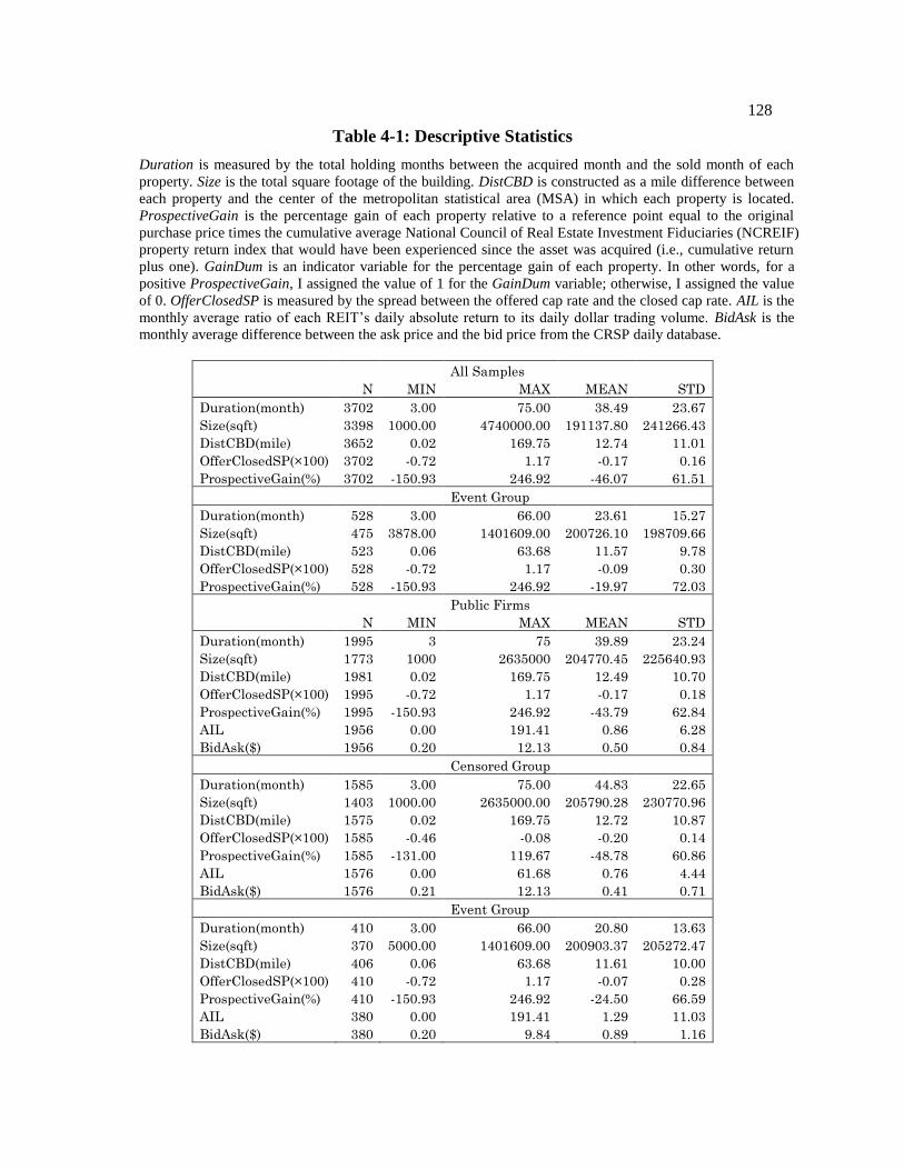
128
Table 4-1: Descriptive Statistics
Duration is measured by the total holding months between the acquired month and the sold month of each
property. Size is the total square footage of the building. DistCBD is constructed as a mile difference between
each property and the center of the metropolitan statistical area (MSA) in which each property is located.
ProspectiveGain is the percentage gain of each property relative to a reference point equal to the original
purchase price times the cumulative average National Council of Real Estate Investment Fiduciaries (NCREIF)
property return index that would have been experienced since the asset was acquired (i.e., cumulative return
plus one). GainDum is an indicator variable for the percentage gain of each property. In other words, for a
positive ProspectiveGain, I assigned the value of 1 for the GainDum variable; otherwise, I assigned the value
of 0. OfferClosedSP is measured by the spread between the offered cap rate and the closed cap rate. AIL is the
monthly average ratio of each REIT’s daily absolute return to its daily dollar trading volume. BidAsk is the
monthly average difference between the ask price and the bid price from the CRSP daily database.
All Samples
N MIN MAX MEAN STD
Duration(month) 3702 3.00 75.00 38.49 23.67
Size(sqft) 3398 1000.00 4740000.00 191137.80 241266.43
DistCBD(mile) 3652 0.02 169.75 12.74 11.01
OfferClosedSP(×100) 3702 -0.72 1.17 -0.17 0.16
ProspectiveGain(%) 3702 -150.93 246.92 -46.07 61.51
Event Group
Duration(month) 528 3.00 66.00 23.61 15.27
Size(sqft) 475 3878.00 1401609.00 200726.10 198709.66
DistCBD(mile) 523 0.06 63.68 11.57 9.78
OfferClosedSP(×100) 528 -0.72 1.17 -0.09 0.30
ProspectiveGain(%) 528 -150.93 246.92 -19.97 72.03
Public Firms
N MIN MAX MEAN STD
Duration(month) 1995 3 75 39.89 23.24
Size(sqft) 1773 1000 2635000 204770.45 225640.93
DistCBD(mile) 1981 0.02 169.75 12.49 10.70
OfferClosedSP(×100) 1995 -0.72 1.17 -0.17 0.18
ProspectiveGain(%) 1995 -150.93 246.92 -43.79 62.84
AIL 1956 0.00 191.41 0.86 6.28
BidAsk($) 1956 0.20 12.13 0.50 0.84
Censored Group
Duration(month) 1585 3.00 75.00 44.83 22.65
Size(sqft) 1403 1000.00 2635000.00 205790.28 230770.96
DistCBD(mile) 1575 0.02 169.75 12.72 10.87
OfferClosedSP(×100) 1585 -0.46 -0.08 -0.20 0.14
ProspectiveGain(%) 1585 -131.00 119.67 -48.78 60.86
AIL 1576 0.00 61.68 0.76 4.44
BidAsk($) 1576 0.21 12.13 0.41 0.71
Event Group
Duration(month) 410 3.00 66.00 20.80 13.63
Size(sqft) 370 5000.00 1401609.00 200903.37 205272.47
DistCBD(mile) 406 0.06 63.68 11.61 10.00
OfferClosedSP(×100) 410 -0.72 1.17 -0.07 0.28
ProspectiveGain(%) 410 -150.93 246.92 -24.50 66.59
AIL 380 0.00 191.41 1.29 11.03
BidAsk($) 380 0.20 9.84 0.89 1.16
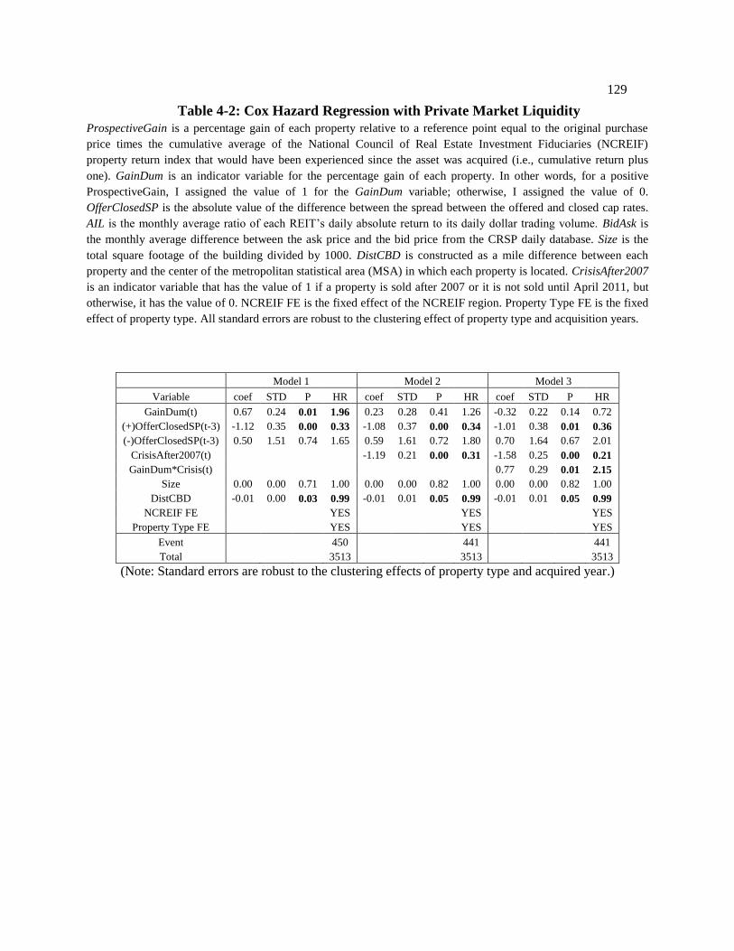
129
Table 4-2: Cox Hazard Regression with Private Market Liquidity
ProspectiveGain is a percentage gain of each property relative to a reference point equal to the original purchase
price times the cumulative average of the National Council of Real Estate Investment Fiduciaries (NCREIF)
property return index that would have been experienced since the asset was acquired (i.e., cumulative return plus
one). GainDum is an indicator variable for the percentage gain of each property. In other words, for a positive
ProspectiveGain, I assigned the value of 1 for the GainDum variable; otherwise, I assigned the value of 0.
OfferClosedSP is the absolute value of the difference between the spread between the offered and closed cap rates.
AIL is the monthly average ratio of each REIT’s daily absolute return to its daily dollar trading volume. BidAsk is
the monthly average difference between the ask price and the bid price from the CRSP daily database. Size is the
total square footage of the building divided by 1000. DistCBD is constructed as a mile difference between each
property and the center of the metropolitan statistical area (MSA) in which each property is located. CrisisAfter2007
is an indicator variable that has the value of 1 if a property is sold after 2007 or it is not sold until April 2011, but
otherwise, it has the value of 0. NCREIF FE is the fixed effect of the NCREIF region. Property Type FE is the fixed
effect of property type. All standard errors are robust to the clustering effect of property type and acquisition years.
(Note: Standard errors are robust to the clustering effects of property type and acquired year.)
Model 1 Model 2 Model 3
Variable coef STD P HR coef STD P HR coef STD P HR
GainDum(t) 0.67 0.24 0.01 1.96 0.23 0.28 0.41 1.26 -0.32 0.22 0.14 0.72
(+)OfferClosedSP(t-3) -1.12 0.35 0.00 0.33 -1.08 0.37 0.00 0.34 -1.01 0.38 0.01 0.36
(-)OfferClosedSP(t-3) 0.50 1.51 0.74 1.65 0.59 1.61 0.72 1.80 0.70 1.64 0.67 2.01
CrisisAfter2007(t)
-1.19 0.21 0.00 0.31 -1.58 0.25 0.00 0.21
GainDum*Crisis(t)
0.77 0.29 0.01 2.15
Size 0.00 0.00 0.71 1.00 0.00 0.00 0.82 1.00 0.00 0.00 0.82 1.00
DistCBD -0.01 0.00 0.03 0.99 -0.01 0.01 0.05 0.99 -0.01 0.01 0.05 0.99
NCREIF FE
YES
YES
YES
Property Type FE
YES
YES
YES
Event
450
441
441
Total
3513
3513
3513
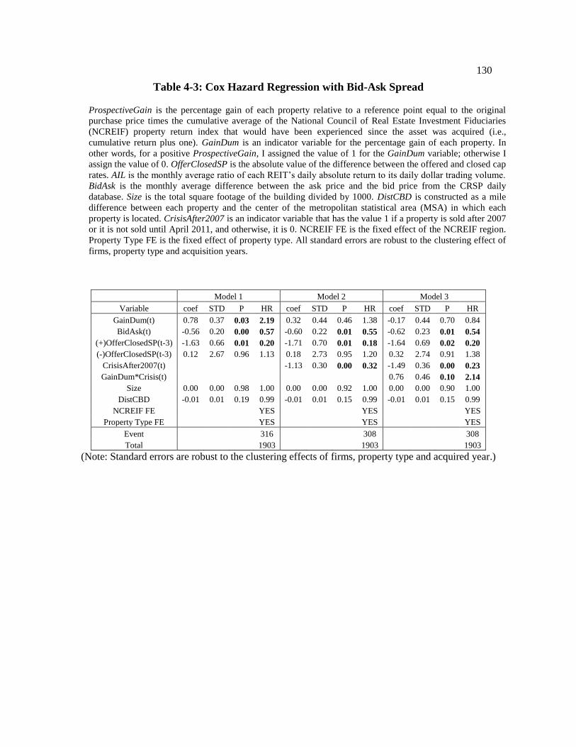
130
Table 4-3: Cox Hazard Regression with Bid-Ask Spread
ProspectiveGain is the percentage gain of each property relative to a reference point equal to the original
purchase price times the cumulative average of the National Council of Real Estate Investment Fiduciaries
(NCREIF) property return index that would have been experienced since the asset was acquired (i.e.,
cumulative return plus one). GainDum is an indicator variable for the percentage gain of each property. In
other words, for a positive ProspectiveGain, I assigned the value of 1 for the GainDum variable; otherwise I
assign the value of 0. OfferClosedSP is the absolute value of the difference between the offered and closed cap
rates. AIL is the monthly average ratio of each REIT’s daily absolute return to its daily dollar trading volume.
BidAsk is the monthly average difference between the ask price and the bid price from the CRSP daily
database. Size is the total square footage of the building divided by 1000. DistCBD is constructed as a mile
difference between each property and the center of the metropolitan statistical area (MSA) in which each
property is located. CrisisAfter2007 is an indicator variable that has the value 1 if a property is sold after 2007
or it is not sold until April 2011, and otherwise, it is 0. NCREIF FE is the fixed effect of the NCREIF region.
Property Type FE is the fixed effect of property type. All standard errors are robust to the clustering effect of
firms, property type and acquisition years.
Model 1 Model 2 Model 3
Variable coef STD P HR coef STD P HR coef STD P HR
GainDum(t) 0.78 0.37 0.03 2.19 0.32 0.44 0.46 1.38 -0.17 0.44 0.70 0.84
BidAsk(t) -0.56 0.20 0.00 0.57 -0.60 0.22 0.01 0.55 -0.62 0.23 0.01 0.54
(+)OfferClosedSP(t-3) -1.63 0.66 0.01 0.20 -1.71 0.70 0.01 0.18 -1.64 0.69 0.02 0.20
(-)OfferClosedSP(t-3) 0.12 2.67 0.96 1.13 0.18 2.73 0.95 1.20 0.32 2.74 0.91 1.38
CrisisAfter2007(t)
-1.13 0.30 0.00 0.32 -1.49 0.36 0.00 0.23
GainDum*Crisis(t)
0.76 0.46 0.10 2.14
Size 0.00 0.00 0.98 1.00 0.00 0.00 0.92 1.00 0.00 0.00 0.90 1.00
DistCBD -0.01 0.01 0.19 0.99 -0.01 0.01 0.15 0.99 -0.01 0.01 0.15 0.99
NCREIF FE
YES
YES
YES
Property Type FE
YES
YES
YES
Event
316
308
308
Total
1903
1903
1903
(Note: Standard errors are robust to the clustering effects of firms, property type and acquired year.)

131
Table 4-4: Cox Hazard Regression with Prospective Gain and Bid-Ask Spread
ProspectiveGain is a percentage gain of each property relative to a reference point equal to the original
purchase price times the cumulative average of the National Council of Real Estate Investment Fiduciaries
(NCREIF) property return index that would have been experienced since the asset was acquired (i.e.,
cumulative return plus one). GainDum is an indicator variable for the percentage gain of each property. In
other words, for a positive ProspectiveGain, I assigned the value of 1 for the GainDum variable; otherwise I
assign the value of 0. OfferClosedSP is the absolute value of the difference between the offered and closed cap
rates. AIL is the monthly average ratio of each REIT’s daily absolute return to its daily dollar trading volume.
BidAsk is the monthly average difference between the ask price and the bid price from the CRSP daily
database. Size is the total square footage of the building divided by 1000. DistCBD is constructed as a mile
difference between each property and the center of the metropolitan statistical area (MSA) in which each
property is located. CrisisAfter2007 is an indicator variable that has the value of 1 if a property is sold after
2007 or it is not sold until April 2011, but otherwise, it has the value of 0. NCREIF FE is the fixed effect of
the NCREIF region. Property Type FE is the fixed effect of property type. All standard errors are robust to the
clustering effect of firms, property type and acquisition years.
Model 1 Model 2 Model 3
Variable coef STD P HR coef STD P HR coef STD P HR
ProspectiveGain(t) 0.00 0.00 0.02 1.00 0.00 0.00 0.73 1.00 0.00 0.00 0.22 1.00
BidAsk(t) -0.57 0.21 0.01 0.57 -0.59 0.22 0.01 0.56 -0.60 0.23 0.01 0.55
(+)OfferClosedSP(t-3) -1.47 0.64 0.02 0.23 -1.78 0.69 0.01 0.17 -1.79 0.69 0.01 0.17
(-)OfferClosedSP(t-3) 0.21 2.68 0.94 1.24 0.10 2.74 0.97 1.10 0.23 2.76 0.93 1.26
CrisisAfter2007(t)
-1.19 0.32 0.00 0.30 -1.70 0.49 0.00 0.18
GainDum*Crisis(t)
0.96 0.56 0.09 2.61
Size 0.00 0.00 0.94 1.00 0.00 0.00 0.91 1.00 0.00 0.00 0.87 1.00
DistCBD -0.01 0.01 0.18 0.99 -0.01 0.01 0.16 0.99 -0.01 0.01 0.16 0.99
NCREIF FE
YES
YES
YES
Property Type FE
YES
YES
YES
Event
316
308
308
Total
1903
1903
1903
(Note: Standard errors are robust to the clustering effects of firms, property type and acquired year.)
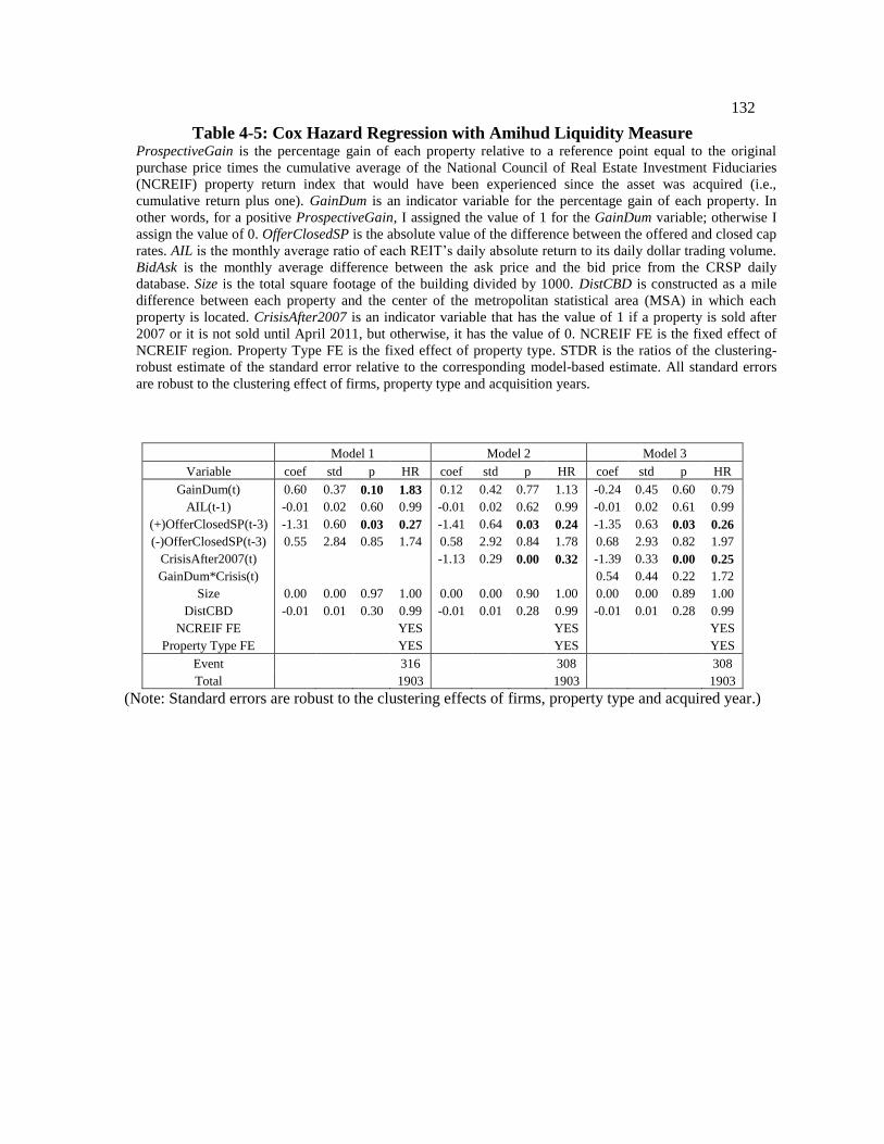
132
Table 4-5: Cox Hazard Regression with Amihud Liquidity Measure ProspectiveGain is the percentage gain of each property relative to a reference point equal to the original
purchase price times the cumulative average of the National Council of Real Estate Investment Fiduciaries
(NCREIF) property return index that would have been experienced since the asset was acquired (i.e.,
cumulative return plus one). GainDum is an indicator variable for the percentage gain of each property. In
other words, for a positive ProspectiveGain, I assigned the value of 1 for the GainDum variable; otherwise I
assign the value of 0. OfferClosedSP is the absolute value of the difference between the offered and closed cap
rates. AIL is the monthly average ratio of each REIT’s daily absolute return to its daily dollar trading volume.
BidAsk is the monthly average difference between the ask price and the bid price from the CRSP daily
database. Size is the total square footage of the building divided by 1000. DistCBD is constructed as a mile
difference between each property and the center of the metropolitan statistical area (MSA) in which each
property is located. CrisisAfter2007 is an indicator variable that has the value of 1 if a property is sold after
2007 or it is not sold until April 2011, but otherwise, it has the value of 0. NCREIF FE is the fixed effect of
NCREIF region. Property Type FE is the fixed effect of property type. STDR is the ratios of the clustering-
robust estimate of the standard error relative to the corresponding model-based estimate. All standard errors
are robust to the clustering effect of firms, property type and acquisition years.
Model 1 Model 2 Model 3
Variable coef std p HR coef std p HR coef std p HR
GainDum(t) 0.60 0.37 0.10 1.83 0.12 0.42 0.77 1.13 -0.24 0.45 0.60 0.79
AIL(t-1) -0.01 0.02 0.60 0.99 -0.01 0.02 0.62 0.99 -0.01 0.02 0.61 0.99
(+)OfferClosedSP(t-3) -1.31 0.60 0.03 0.27 -1.41 0.64 0.03 0.24 -1.35 0.63 0.03 0.26
(-)OfferClosedSP(t-3) 0.55 2.84 0.85 1.74 0.58 2.92 0.84 1.78 0.68 2.93 0.82 1.97
CrisisAfter2007(t)
-1.13 0.29 0.00 0.32 -1.39 0.33 0.00 0.25
GainDum*Crisis(t)
0.54 0.44 0.22 1.72
Size 0.00 0.00 0.97 1.00 0.00 0.00 0.90 1.00 0.00 0.00 0.89 1.00
DistCBD -0.01 0.01 0.30 0.99 -0.01 0.01 0.28 0.99 -0.01 0.01 0.28 0.99
NCREIF FE
YES
YES
YES
Property Type FE
YES
YES
YES
Event
316
308
308
Total
1903
1903
1903
(Note: Standard errors are robust to the clustering effects of firms, property type and acquired year.)
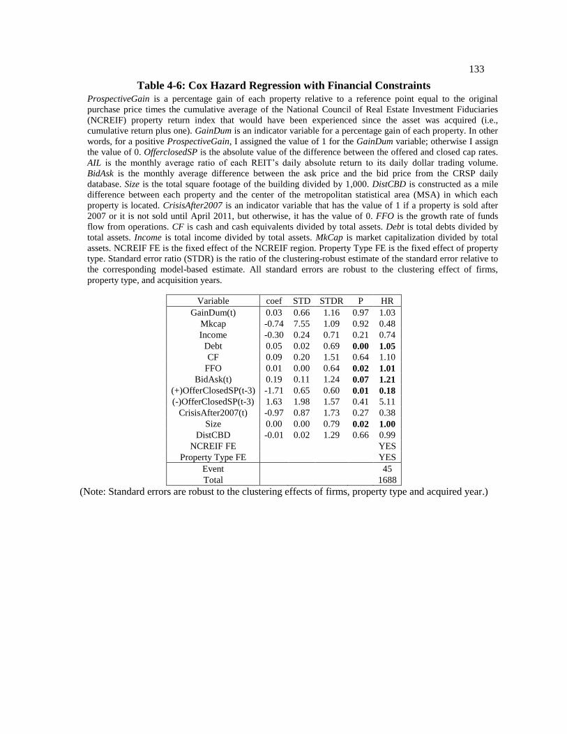
133
Table 4-6: Cox Hazard Regression with Financial Constraints
ProspectiveGain is a percentage gain of each property relative to a reference point equal to the original
purchase price times the cumulative average of the National Council of Real Estate Investment Fiduciaries
(NCREIF) property return index that would have been experienced since the asset was acquired (i.e.,
cumulative return plus one). GainDum is an indicator variable for a percentage gain of each property. In other
words, for a positive ProspectiveGain, I assigned the value of 1 for the GainDum variable; otherwise I assign
the value of 0. OfferclosedSP is the absolute value of the difference between the offered and closed cap rates.
AIL is the monthly average ratio of each REIT’s daily absolute return to its daily dollar trading volume.
BidAsk is the monthly average difference between the ask price and the bid price from the CRSP daily
database. Size is the total square footage of the building divided by 1,000. DistCBD is constructed as a mile
difference between each property and the center of the metropolitan statistical area (MSA) in which each
property is located. CrisisAfter2007 is an indicator variable that has the value of 1 if a property is sold after
2007 or it is not sold until April 2011, but otherwise, it has the value of 0. FFO is the growth rate of funds
flow from operations. CF is cash and cash equivalents divided by total assets. Debt is total debts divided by
total assets. Income is total income divided by total assets. MkCap is market capitalization divided by total
assets. NCREIF FE is the fixed effect of the NCREIF region. Property Type FE is the fixed effect of property
type. Standard error ratio (STDR) is the ratio of the clustering-robust estimate of the standard error relative to
the corresponding model-based estimate. All standard errors are robust to the clustering effect of firms,
property type, and acquisition years.
Variable coef STD STDR P HR
GainDum(t) 0.03 0.66 1.16 0.97 1.03
Mkcap -0.74 7.55 1.09 0.92 0.48
Income -0.30 0.24 0.71 0.21 0.74
Debt 0.05 0.02 0.69 0.00 1.05
CF 0.09 0.20 1.51 0.64 1.10
FFO 0.01 0.00 0.64 0.02 1.01
BidAsk(t) 0.19 0.11 1.24 0.07 1.21
(+)OfferClosedSP(t-3) -1.71 0.65 0.60 0.01 0.18
(-)OfferClosedSP(t-3) 1.63 1.98 1.57 0.41 5.11
CrisisAfter2007(t) -0.97 0.87 1.73 0.27 0.38
Size 0.00 0.00 0.79 0.02 1.00
DistCBD -0.01 0.02 1.29 0.66 0.99
NCREIF FE
YES
Property Type FE
YES
Event
45
Total
1688
(Note: Standard errors are robust to the clustering effects of firms, property type and acquired year.)

134
Chapter 5
Concluding Remarks
In this dissertation, I investigate market frictions in the real estate market by focusing
on two topics: liquidity and segmentation.
Chapter 2 contributes to the existing literature by concentrating on the dynamics of
liquidity between the private and public real estate markets. First, by focusing on real estate
markets, I am able to incorporate the liquidity of underlying assets into the private market.
The commercial real estate market is considered relatively illiquid because market
segmentation reflects heterogeneous locations and property types. Accordingly, liquidity
shocks and their patterns in the real estate market require a specific analysis—one that
focuses only on real estate markets.
Second, by identifying the liquidity impact of the private market, I obtain additional
insights into the relationship between the private and public real estate markets. Though the
risk and adjusted-return relationship between the private and public real estate markets is
well documented, few studies have concentrated on the dynamics of liquidity between the
two markets. Thus, my study has important implications for portfolio management and
investment allocations as any given liquidity shock may have an interdependent effect on
the private and public markets. If investors were to be made aware that a liquidity shock has
an interdependent effect on private and public markets, they would be able to refine their
risk-management strategies accordingly and manage their portfolios based on

135
correspondingly better predictions of the liquidity patterns across real estate markets.
Chapter 3 empirically tests whether the law of one price holds for an important class of
heterogeneous assets: commercial real estate. More specifically, I consider these questions:
Does average pricing differ by investor type? If average pricing does not differ, does the
same asset have more than one factor price? If each investor transacts for the same asset but
each does so in a different domain, is the factor price of the heterogeneous assets
discontinuous? In proposing answers to these research questions, I provide empirical
evidence regarding the existence of market segmentation in the commercial real estate
market. I depart from the literature in several ways. First, using six investor types, I
specified three types of market segmentation in the commercial real estate market. Second,
I proposed a sequential testing process for market segmentation. My testing procedure
allows me to make a precise comparison between the treated group and the control group
given the same propensity score in terms of property and location characteristics. Thus, I
address the issue of market segmentation by investor type in a more rigorous way than in
the previous literature. To my knowledge, few studies have directly examined pricing
differences across investor types using a sequential testing procedure.
Chapter 4 addresses the issue of loss aversion and market liquidity. The link between
market liquidity and loss-aversion behavior is important to at least beginning to
comprehend a few puzzling patterns in the real estate market: Why does the real estate
market show a positive correlation between prices and liquidity throughout the housing
cycle? Why are sellers reluctant to reduce their asking price in a market downturn? If
market liquidity amplifies the loss aversion of sellers, the interaction between liquidity and
loss aversion can partially explain the co-movement of prices and liquidity in the real estate

136
market. My empirical results suggest that loss-aversion behavior becomes more pronounced
in a less-liquid market and that this may provide an explanation as to why the real estate
market shows a sudden loss of liquidity in a market downturn.
Furthermore, the link between market liquidity and loss aversion provides insights into
investment and risk-management strategies: Given the interaction between market liquidity
and loss aversion, the actual investment risk may be more significant than expected. Thus,
understanding the link between market liquidity and loss-aversion behavior can help
investors become aware of the dynamics of liquidity in the real estate market.
Additionally, my empirical results are important in that the previous literature on loss
aversion does not cover the crisis period of 2007–2008. I demonstrate that if sellers are not
willing to sell their property for a potential gain in a market downturn, loss aversion and
disposition effect do not hold in a market downturn. And, therefore, the impact of loss
aversion on the sale probability should be understood in a different way―a way that takes
relative market liquidity into account.
In summary, this dissertation demonstrates that the real estate market is constrained by
market frictions, and it provides empirical evidence regarding the dynamics of liquidity and
market segmentation in the commercial real estate market. This research provides key
insights into understanding the impact of market frictions and the ways in which they call
into question the principles of classical economics.

137
Bibliography
Acharya, V.V., and L.H. Pedersen. (2005). Asset Pricing with Liquidity Risk. Journal of
Financial Economics 77(2): 375–410.
Akin, S. N., V. E. Lambson, G. R. McQueen, B. Platt, B.A. Slade and J. Wood. (2011). Rushing
to Overpay: The REIT Premium Revisited. Unpublished manuscript.
Amihud, Y.I. (2002). Liquidity and Stock Returns: Cross-Section and Time-Series Effects.
Journal of Financial Markets 5(1): 31–56.
Anenberg, E. (2011). Loss Aversion, Equity Constraints and Seller Behavior in the Real Estate
Market. Regional Science and Urban Economics 41(2011): 67–76
Bao, J., J. Pan and J. Wang. (2011). The Illiquidity of Corporate Bonds. Journal of Finance
66(3): 911–946.
Benartzi, S. and R. Thaler. (1995). Myopic Loss Aversion and the Equity Premium Puzzle.
Quarterly Journal of Economics 110: 73–92.
Benveniste, L., D.R. Capozza, and P.J. Seguin. (2001). The Value of Liquidity. Real Estate
Economics 29(4): 633–660.
Bokhari, S. and D. Geltner.(2011). Loss Aversion and Anchoring in Commercial Real Estate
Pricing. Real Estate Economics 39(4): 635–670.
Bond, S.A. and Q. Chang. (2011). Liquidity Dynamics Across Public and Private
Markets.Unpublished manuscript.
Brounen, D., P. Eichholtz, and D.T. Ling. (2009). The Liquidity of Property Shares: An
International Comparison. Real Estate Economics 37(3): 413–445.
Brown, D.T. (2000). Liquidity and Liquidation: Evidence from Real Estate Investment Trusts.
Journal of Finance 55(1): 469–485.
Brunnermeier, M., and L. Pedersen. (2009). Market Liquidity and Funding Liquidity. Review of
Financial Studies 26(6): 2201–2238.
Calvo, G.A. and E.G. Mendoza. (2000). Rational Contagion and the Globalization of Securities
Markets. Journal of International Economics 51: 79–113.
Chorida, T., A. Sarkar and A. Subrahmanyam. (2005). An Empirical Analysis of Stock and
Bond Market Liquidity. Review of Financial Studies 18: 85–129.
Clayton, J., G. MacKinnon and L. Peng. (2008). Time Variation of Liquidity in the Private Real

138
Estate Market: An Empirical Investigation. Journal of Real Estate Research 30(2): 125–
160.
Cochrane, J.H. (2011). Presidential Address: Discount Rates. Journal of Finance 66(4): 1047–
1108.
Collin-Dufresne, P., R.S. Goldstein and J.S. Martin. (2001). The Determinants of Credit Spread
Changes. Journal of Finance 56(6): 2177–2207.
Cox, D. R. (1972). Regression Models and Life-Tables (with discussion), Journal of the Royal
Statistical Society 34: 187–220.
Crane, A. and J. Hartzell. (2009). Is There a Disposition Effect in Corporate Investment
Decisions? Evidence from Real Estate Investment Trusts. The University of Texas at
Austin. Unpublished manuscript.
Dickey, D. A. and W.A. Fuller. (1981). Likelihood Ratio Statistics for Autoregressive Time
Series with A Unit Root. Econometrica 49(4): 1057–1072.
Ekeland, I., J.J. Heckman and L. Nesheim. (2002). Identifying Hedonic Models. America
Economic Review 92(2): 304–309.
Engelhardt., G.V. (2003). Nominal Loss Aversion, Housing Equity Constraints, and Household
Mobility: Evidence from the United States. Journal of Urban Economics 53: 171–195.
Epple, D. (1987). Hedonic Prices and Implicit Markets: Estimating Demand and Supply
Functions for Differentiated Products. Journal of Political Economy 95 (1): 59–80.
Genesove. D. and C. Myer. (2001). Loss Aversion and Seller Behavior: Evidence from the
Housing Market. Quarterly Journal of Economics 166: 1233–1260.
Fisher, J., D. Gatzlaff, D. Geltner and D. Haurin. (2003). Controlling for the Impact of Variable
Liquidity in Commercial Real Estate Price Indices. Real Estate Economics 31(2): 269–303.
Goldstein,I., and A. Pauzner. (2004). Contagion of Self-Fulfilling Financial Crises due to
Diversification of Investment Portfolios. Journal of Economic Theory 119: 151–183.
Gromb, D. and D. Vayanos. (2010). Limits of Arbitrage. Annual Review of Financial Economics
2: 251–275.
Hardin, W., and M. Wolverston. (1999). Equity REIT Property Acquisitions: Do Apartment
REITs Pay a Premium? Journal of Real Estate Research 17(1/2): 113–126.
Harding, J. P., J.R. Knight, and C.F. Sirmans. (2003). Estimating Bargaining Effects in Hedonic
Models: Evidence from the Housing Market. Real Estate Economics 31(4): 601–622.
Hartmann, P., S. Straetmans and C.G. de Vries. (2004). Asset Market Linkages in Crisis Periods.

139
The Review of Economics and Statistics 86(1): 313–326.
Holmes, A., and B. Slade. (2001). Do Tax-Deferred Exchanges Impact Purchase Price?
Evidence for the Phoenix Apartment Market. Real Estate Economics 29(4): 567–588.
Huang, X., H. Zhou and H. Zhu. (2009). A Framework for Assessing the Systemic Risk of
Major Financial Institutions. Journal of Banking & Finance 33(11): 2036–2049.
Jacoby, G., G.J. Jiang and G. Theocharides. (2010). Cross-Market Liquidity Shocks: Evidence
from the CDS, Corporate Bond and Equity Market. Unpublished manuscript.
Kahneman, D. and A. Tversky. (1979). Prospect Theory: An Analysis of Decision under Risk.
Econometrica 47: 263–291.
King, M., and S. Wadhwani. (1990). Transmission of Volatility Between Stock Markets. Review
of Financial Studies 3: 5–33.
Kodres, L., and M. Pritsker. (2002). A Rational Expectations Model of Financial Contagion.
Journal of Finance 57: 769–799.
Krainer. J. (2001). A Theory of Liquidity in Residential Real Estate Markets. Journal of Urban
Economics 49: 32–53.
Kumar, P., and D. Seppi. (1994). Information and Index Arbitrage. Journal of Business 67(4):
481–509.
Kyle, A.S. (1985). Continuous Auctions and Insider Trading. Econometrica 53(6): 1315–1335.
Lamont, O. and R. Thaler. (2003). Can the Market Add and Subtract? Mispricing in Tech Stock
Carve-Outs. Journal of Political Economy 111: 227–268.
Lamont. O. and J.C. Stein. (1999). Leverage and House-Price Dynamics in U.S. Cities. The
RAND Journal of Economics 30(3): 498–514.
Lien, D. and K.Shrestha. (2011). Price Discovery in Interrelated Markets. Unpublished
manuscript.
Lin, Z., and K.D. Vandell. (2007). Illiquidity and Pricing Biases in the Real Estate Market. Real
Estate Economics 35(3): 291–330.
Ling, D. C., and M. Petrova. (2010). Heterogeneous Investors, Negotiation Strength and Asset
Prices in Private Markets: Evidence from Commercial Real Estate. Unpublished
manuscript.
Ling, D.C., A. Naranjo and B. Scheick. (2011). Funding Constraints and Commercial Real
Estate Pricing Spirals. Unpublished manuscript.

140
O'Hara, M. (1995). Market microstructure theory, Malden, MA: Blackwell.
Ong. S.E., Neo. P. H. and Y. Tu. (2008). Foreclosure Sales: The Effects of Price Expectations,
Volatility and Equity Losses. Journal of Real Estate Finance and Economics 36: 265–287.
Pagliari, J.L., K.A.Scherer and R.T. Monopoli. (2005). Public versus Private Real Estate
Equities: A More Refined, Long-Term Comparison. Real Estate Economics 33(1): 147–
187.
Pan, J., and K. Singleton. (2008). Default and Recovery Implicit in the Term Structure of
Sovereign CDS Spreads. Journal of Finance 63(5): 2345–2384.
Pliska, S. R. (1997). Introduction to mathematical finance: Discrete time models. Wiley.
Rosenthal, L. and C. Young. (1990). The Seemingly Anomalous Price Behavior of Royal
Dutch/Shell and Unilever N.V./PLC. Journal of Financial Economics 26: 123–141.
Rosen, S. (1974). Hedonic Prices and Implicit Markets: Product Differentiation in Pure
Competition. Journal of Political Economy 82(1): 34–55.
Sharpe, W., and G.J. Alexander. (1990). Investments. 4th
edition. Prentice Hall.
Shefrin. H. and M. Statman. (1985). The Disposition to Sell Winners Too Early and Ride Losers
Too Long: Theory and Evidence. Journal of Finance 40(3): 777–790.
Shleifer, A., and R.W. Vishny. (1997). The Limits of Arbitrage. Journal of Finance 52(1):
35−55.
Subrahmanyam, A. (1991). Risk Aversion, Market Liquidity, and Price Efficiency. The Review
of Financial Studies 4(3): 417–441.
Tu. Y., Ong. S.E. and Y.H. Han. (2009). Turnovers and Housing Price Dynamics: Evidence
from Singapore Condominium Market. Journal of Real Estate Finance and Economics 38:
254–274.
Vayanos, D. (2004). Flight to Quality, Flight to Liquidity, and the Pricing of Risk. Working
Paper. MIT.
Wooldridge, J.M. (2002) Econometric Analysis of Cross Section and Panel Data. The MIT
Press.
Yuan, K.(2002). Asymmetric Price Movements and Borrowing Constraints: A Rational
Expectations Equilibrium Model of Crises, Contagion and Confusion. Unpublished
manuscript.
Zhang, B.Y., H. Zhou and H. Zhu. (2009). Explaining Credit Default Swap Spreads with the
Equity Volatility and Jump Risks of Individual Firms. Review of Financial Studies 22(12):
5099–5131.

VITA
Sun Young Park
Smeal College of Business Administration Email: [email protected]
Department of Risk Management, 360A Business Building Tel: (814) 863-5454 (office)
The Pennsylvania State University, University Park, PA 16802 (716) 908-4346 (mobile)
EDUCATION
Pennsylvania State Universi ty University Park, PA
Ph.D. i n Business 2008–2012
– Dissertation: Essays on Market Frictions in the Real Estate Market
State Univers ity of New York at Buffalo Buffalo, NY
M.A. in Economics 2005–2008
Seoul National University Seoul, Korea
B.A. in Education 1995–1999
RESEARCH INTERESTS
Investments, Real Estate Finance, International Finance and Capital Markets
COMPETITIVE RESEARCH GRANTS
2011 Real Estate Research Institute (RERI) Research Grant (with Dr. Brent W. Ambrose)
2009-2011 Smeal College of Business Research Grant, Pennsylvania State University
HONORS AND AWARDS
2011 The Peter E. Liberti and Judy D. Olian Scholarship, Pennsylvania State University
2008–present Tuition Scholarship and Teaching Assistantship, Pennsylvania State University
2005–2008 Tuition Scholarship and Fellowship, State University of New York at Buffalo
CONFERENCE PRESENTATIONS
2012 American Real Estate and Urban Economics Association (AREUEA) Doctoral Session
PROFESSIONAL EXPERIENCE
Instructor
Pennsylvania State University 2010–2012
– Analysis of Real Estate Markets (REST 420)
– Real Estate Fundamentals (REST 301)
Teaching Assistant
Pennsylvania State University 2008–2009
Academic Advisor
State University of New York at Buffalo 2005–2008