Embed Size (px)
Citation preview
University of Massachusetts Amherst University of Massachusetts Amherst
ScholarWorks@UMass Amherst ScholarWorks@UMass Amherst
Doctoral Dissertations Dissertations and Theses
July 2020
ESSAYS ON COMPETITIVE PERISHABLE FOOD SUPPLY CHAIN ESSAYS ON COMPETITIVE PERISHABLE FOOD SUPPLY CHAIN
NETWORKS: FROM THE IMPACTS OF TARIFFS AND QUOTAS TO NETWORKS: FROM THE IMPACTS OF TARIFFS AND QUOTAS TO
INTEGRATION OF QUALITY INTEGRATION OF QUALITY
Deniz Besik University of Massachusetts Amherst
Follow this and additional works at: https://scholarworks.umass.edu/dissertations_2
Part of the Business Administration, Management, and Operations Commons, Management Sciences
and Quantitative Methods Commons, and the Operations and Supply Chain Management Commons
Recommended Citation Recommended Citation Besik, Deniz, "ESSAYS ON COMPETITIVE PERISHABLE FOOD SUPPLY CHAIN NETWORKS: FROM THE IMPACTS OF TARIFFS AND QUOTAS TO INTEGRATION OF QUALITY" (2020). Doctoral Dissertations. 1920. https://doi.org/10.7275/x88v-7073 https://scholarworks.umass.edu/dissertations_2/1920
This Open Access Dissertation is brought to you for free and open access by the Dissertations and Theses at ScholarWorks@UMass Amherst. It has been accepted for inclusion in Doctoral Dissertations by an authorized administrator of ScholarWorks@UMass Amherst. For more information, please contact [email protected].
ESSAYS ON COMPETITIVE PERISHABLEFOOD SUPPLY CHAIN NETWORKS:
FROM THE IMPACTS OF TARIFFS AND QUOTASTO INTEGRATION OF QUALITY
A Dissertation Presented
by
DENIZ BESIK
Submitted to the Graduate School of the
University of Massachusetts Amherst in partial fulfillment
of the requirements for the degree of
DOCTOR OF PHILOSOPHY
May 2020
Isenberg School of Management

c© Copyright by Deniz Besik 2020
All Rights Reserved
ESSAYS ON COMPETITIVE PERISHABLEFOOD SUPPLY CHAIN NETWORKS:
FROM THE IMPACTS OF TARIFFS AND QUOTASTO INTEGRATION OF QUALITY
A Dissertation Presented
by
DENIZ BESIK
Approved as to style and content by:
Anna Nagurney, Chair
Hari Jagannathan Balasubramanian, Member
Priyank Arora, Member
Ana Muriel, Member
George R. Milne, Program DirectorIsenberg School of Management
DEDICATION
To Afife Buyukyilmaz Besik, Orhan Besik, and Elif Zeynep Besik.

ACKNOWLEDGMENTS
I will always be thankful and grateful to my academic advisor and dissertation chair, John F.
Smith Memorial Professor Anna Nagurney, for her support, guidance, and patience during the five
years of my doctoral studies. I would like to thank her especially for accepting me as her doctoral
student which was one of the most rewarding experiences of my life. Under her guidance, I was able
to achieve many milestones and grew intellectually and personally. I will especially remember her
guidance and support for my first publication and my first conference attendance. Her dedication to
her profession, her enthusiasm, energy, and attention to details have always motivated me to work
hard and be better. As a future female academic, I see her as a great role model and a true leader.
I feel extremely lucky to have Professor Nagurney as my advisor.
I would like to thank Professor Hari Balasubramian, Professor Ana Muriel, and Professor Priyank
Arora for their time and providing very helpful comments on my dissertation. I am also very
grateful for their advice and support during the job search process. I would like to thank Professor
Senay Solak, Professor Ahmed Ghoniem, and Professor Christian Rojas for their support during
my coursework, and their advice about academia or life in general. I am also grateful to Professor
Agha Iqbal Ali, Professor Robert Nakosteen and Professor George Milne for helping me through the
program. I also would like to thank Professor Ladimer Nagurney for his support and guidance. In
addition, I want to thank Audrey Kieras, Michael Korza, Priscilla Mayoussier, and Lynda Vassallo
for their administrative assistance. I am also very thankful to Robert Colnes, who passed away in
May 2016. His insights helped me immensely on my first publication.
I was very fortunate to meet many great friends and lab mates throughout my doctoral studies
who eventually became my new family. I am very thankful and grateful to Rodrigo Mercado Fer-
nandez, and Dr. Pritha Dutta for their support, encouragement, and friendship. I am especially
thankful to both of them for their help and patience during my academic job search process. I am
also very grateful for my lab mates, Mojtaba Salarpur, Jianmei Wu, and Meiyu Huang, at the the
Virtual Center for Supernetworks. I really appreciate the support of other Center Associates includ-
ing Dr. Sara Saberi, Dr. Dong ”Michelle” Li, Dr. Min Yu, Dr. June Dong, Dr. Shivani Shukla, Dr.
v

Jose Cruz, and Dr. Dmytro Matsypura who have helped me in many ways at different stages of my
doctoral journey. I am very grateful to my friends in different parts of the US, Dr. Aybike Ulusan,
Dr. Gokce Kahvecioglu, and Can Kucukgul, for their support especially at the conferences. I am
also very thankful to my other friends in Amherst and in Turkey.
Finally, I would like to thank my family. I’d like to thank my mom and my dad for their constant
support, guidance, and being always there for me. I would also like to thank my dad for suggesting
that I study Industrial Engineering in my Bachelor’s which eventually led to a PhD in Management
Science. I am very thankful to my little sister for always listening to me and making jokes to cheer
me up. I am very grateful to the rest of my family including my grandparents, aunts, and uncles
who have been pillars of support and given me strength and encouragement since t = 0.
vi
ABSTRACT
ESSAYS ON COMPETITIVE PERISHABLEFOOD SUPPLY CHAIN NETWORKS:
FROM THE IMPACTS OF TARIFFS AND QUOTASTO INTEGRATION OF QUALITY
MAY 2020
DENIZ BESIK
BACHELOR OF SCIENCE, SABANCI UNIVERSITY
MASTER OF SCIENCE, SABANCI UNIVERSITY
Ph.D., UNIVERSITY OF MASSACHUSETTS AMHERST
Directed by: Professor Anna Nagurney
Food, in the form of fresh produce, meat, fish, and/or dairy, is necessary for maintaining
life. In this dissertation, I focus on the modeling and analysis of some of the inherent issues in
competitive perishable food supply chain networks. I investigate the impacts of trade policies such
as tariffs, quotas, and their combination – tariff-rate quotas, as well as the integration of food quality
deterioration into food supply chains. The research is especially timely given the prevalence of trade
wars and tariffs in todays global political environment. The work is multidisciplinary with constructs
from food science integrated into the economics of supply chain networks.
The first part of the dissertation overviews the methodological foundations including game theory,
network and optimization theory, and variational inequality theory used for the construction and
solution of the supply chain network models. In the second part of the dissertation, I first focus on
perfectly competitive problems and develop a unified variational inequality framework for spatial
vii
price network equilibrium problems with tariff-rate quotas. The accompanying case study on the
dairy industry is based on trade between the United States and France. The computational results
reveal that tariff-rate quotas may protect domestic producers from foreign competition, but at the
expense of higher demand prices for consumers. This work is based on the paper by Nagurney,
Besik, and Dong (2019). I then develop an oligopolistic supply chain network equilibrium model
with differentiated products consisting of multiple firms, production sites, and demand markets, in
which firms compete on product quantities and also quality. I provide a case study on soybeans, an
important agricultural product, and investigate different scenarios. Insights as to firm profits and
trade volumes, the average product quality, and consumer welfare, are also delineated. Specifically,
I find that, although firms may benefit from the imposition of a quota or tariff, the welfare of
consumers in the country imposing the quota or tariff declines. This work is based on the paper by
Nagurney, Besik, and Li (2019).
In the third part of my dissertation, I demonstrate how to incorporate quality deterioration of
fresh produce into perishable supply chain network models. I construct an explicit equation for fresh
produce quality deterioration based on time and temperature of different pathways in supply chain
networks. I first incorporate this feature into local markets in the form of farmers’ markets, which
serve as examples of direct to consumer channels and shorter supply chain networks. I also provide
a case study of apples in western Massachusetts, under various scenarios, including production
disruptions, due to negative weather conditions, resulting in an increase in apple prices at farmers’
markets, a decrease in quality, and a decrease in profits for the apple orchards. These results can
be used to inform food firms, policy makers, and regulators. This work is based on the paper by
Besik and Nagurney (2017). Subsequently, I develop a competitive food supply chain network model
in which the profit-maximizing producers decide not only as to the volume of fresh produce, but
they also decide on the initial quality of fresh produce, with associated costs. I incorporate quality
deterioration of the fresh produce explicitly with chemical functions depending on time, temperature,
and the initial quality of the food product. I then present a case study on peaches, with supply
chain disruptions to reveal valuable insights. I find that the disruptions in production result in
higher demand prices, and lower initial quality. This is the first such general supply chain network
model constructed to include the initial quality of fresh produce. This part of the dissertation is
based on the paper by Nagurney, Besik, and Yu (2018).
viii
TABLE OF CONTENTS
Page
ACKNOWLEDGMENTS . . . . . . . . . . . . . . . . . . . . . . . . . . . . . . . . . . . . . . . . . . . . . . . . . . . . . . . . . . . v
ABSTRACT . . . . . . . . . . . . . . . . . . . . . . . . . . . . . . . . . . . . . . . . . . . . . . . . . . . . . . . . . . . . . . . . . . . . . . . vii
LIST OF TABLES . . . . . . . . . . . . . . . . . . . . . . . . . . . . . . . . . . . . . . . . . . . . . . . . . . . . . . . . . . . . . . . . xiv
LIST OF FIGURES . . . . . . . . . . . . . . . . . . . . . . . . . . . . . . . . . . . . . . . . . . . . . . . . . . . . . . . . . . . . . xviii
CHAPTER
1. INTRODUCTION AND RESEARCH MOTIVATION . . . . . . . . . . . . . . . . . . . . . . . . . . . 1
1.1 Trade and Policy Instruments . . . . . . . . . . . . . . . . . . . . . . . . . . . . . . . . . . . . . . . . . . . . . . . . . . 3
1.2 Perishable Food Supply Chains . . . . . . . . . . . . . . . . . . . . . . . . . . . . . . . . . . . . . . . . . . . . . . . . . 6
1.2.1 Quality of Food Products . . . . . . . . . . . . . . . . . . . . . . . . . . . . . . . . . . . . . . . . . . . . . . . 6
1.3 Literature Review . . . . . . . . . . . . . . . . . . . . . . . . . . . . . . . . . . . . . . . . . . . . . . . . . . . . . . . . . . . . . 7
1.3.1 Perfectly and Imperfectly Competitive Models for Agricultural TradeProblems . . . . . . . . . . . . . . . . . . . . . . . . . . . . . . . . . . . . . . . . . . . . . . . . . . . . . . . . . . . 8
1.3.1.1 Spatial Price Equilibrium Models . . . . . . . . . . . . . . . . . . . . . . . . . . . . . . . . . 8
1.3.1.2 Oligopolistic Models . . . . . . . . . . . . . . . . . . . . . . . . . . . . . . . . . . . . . . . . . . . . 9
1.3.2 Product Quality in Perishable Food Supply Chains . . . . . . . . . . . . . . . . . . . . . . . . . 10
1.3.3 Modeling of Quality in the Presence of Tariffs and Quotas . . . . . . . . . . . . . . . . . . . 12
1.4 Dissertation Overview. . . . . . . . . . . . . . . . . . . . . . . . . . . . . . . . . . . . . . . . . . . . . . . . . . . . . . . . . 12
ix
1.4.1 Contributions in Chapter 3 . . . . . . . . . . . . . . . . . . . . . . . . . . . . . . . . . . . . . . . . . . . . . . 12
1.4.2 Contributions in Chapter 4 . . . . . . . . . . . . . . . . . . . . . . . . . . . . . . . . . . . . . . . . . . . . . . 14
1.4.3 Contributions in Chapter 5 . . . . . . . . . . . . . . . . . . . . . . . . . . . . . . . . . . . . . . . . . . . . . . 15
1.4.4 Contributions in Chapter 6 . . . . . . . . . . . . . . . . . . . . . . . . . . . . . . . . . . . . . . . . . . . . . . 16
1.4.5 Concluding Comments . . . . . . . . . . . . . . . . . . . . . . . . . . . . . . . . . . . . . . . . . . . . . . . . . . 17
2. METHODOLOGIES . . . . . . . . . . . . . . . . . . . . . . . . . . . . . . . . . . . . . . . . . . . . . . . . . . . . . . . . . . . . 19
2.1 Variational Inequality Theory . . . . . . . . . . . . . . . . . . . . . . . . . . . . . . . . . . . . . . . . . . . . . . . . . . 19
2.2 The Relationships between Variational Inequalities and Game Theory . . . . . . . . . . . . . . . 24
2.3 Generalized Nash Equilibrium (GNE) . . . . . . . . . . . . . . . . . . . . . . . . . . . . . . . . . . . . . . . . . . . 26
2.4 Algorithms . . . . . . . . . . . . . . . . . . . . . . . . . . . . . . . . . . . . . . . . . . . . . . . . . . . . . . . . . . . . . . . . . . 27
2.4.1 The Euler Method . . . . . . . . . . . . . . . . . . . . . . . . . . . . . . . . . . . . . . . . . . . . . . . . . . . . . 27
2.4.2 The Modified Projection Method . . . . . . . . . . . . . . . . . . . . . . . . . . . . . . . . . . . . . . . . . 29
3. TARIFFS AND QUOTAS IN WORLD TRADE: A UNIFIEDVARIATIONAL INEQUALITY FRAMEWORK . . . . . . . . . . . . . . . . . . . . . . . . . . . . 31
3.1 The Spatial Price Network Equilibrium Model with Tariff Rate Quotas . . . . . . . . . . . . . . 31
3.2 Variants of the Spatial Price Network Equilibrium Model . . . . . . . . . . . . . . . . . . . . . . . . . . 39
3.2.1 Illustrative Examples . . . . . . . . . . . . . . . . . . . . . . . . . . . . . . . . . . . . . . . . . . . . . . . . . . . 42
3.2.1.1 Illustrative Example 1 . . . . . . . . . . . . . . . . . . . . . . . . . . . . . . . . . . . . . . . . . . 42
3.2.1.2 Illustrative Example 2 . . . . . . . . . . . . . . . . . . . . . . . . . . . . . . . . . . . . . . . . . . 44
3.3 Qualitative Properties . . . . . . . . . . . . . . . . . . . . . . . . . . . . . . . . . . . . . . . . . . . . . . . . . . . . . . . . 45
3.4 The Algorithm . . . . . . . . . . . . . . . . . . . . . . . . . . . . . . . . . . . . . . . . . . . . . . . . . . . . . . . . . . . . . . 48
3.4.1 Closed Form Expressions . . . . . . . . . . . . . . . . . . . . . . . . . . . . . . . . . . . . . . . . . . . . . . . . 49
3.5 A Case Study on the Dairy Industry . . . . . . . . . . . . . . . . . . . . . . . . . . . . . . . . . . . . . . . . . . . 50
3.5.1 Baseline Example . . . . . . . . . . . . . . . . . . . . . . . . . . . . . . . . . . . . . . . . . . . . . . . . . . . . . . 51
3.5.2 Change in Quotas Example . . . . . . . . . . . . . . . . . . . . . . . . . . . . . . . . . . . . . . . . . . . . . 56
x
3.5.3 Increase in the Number of Paths Example . . . . . . . . . . . . . . . . . . . . . . . . . . . . . . . . . 59
3.6 Summary and Conclusions . . . . . . . . . . . . . . . . . . . . . . . . . . . . . . . . . . . . . . . . . . . . . . . . . . . . . 63
4. STRICT QUOTAS OR TARIFFS? IMPLICATIONS FOR PRODUCTQUALITY AND CONSUMER WELFARE IN DIFFERENTIATEDPRODUCT SUPPLY CHAINS . . . . . . . . . . . . . . . . . . . . . . . . . . . . . . . . . . . . . . . . . . . . . . 65
4.1 The Differentiated Product Supply Chain Network Equilibrium Models withQuality . . . . . . . . . . . . . . . . . . . . . . . . . . . . . . . . . . . . . . . . . . . . . . . . . . . . . . . . . . . . . . . . . . 66
4.1.1 The Differentiated Product Supply Chain Network Equilibrium Modelwithout Trade Interventions . . . . . . . . . . . . . . . . . . . . . . . . . . . . . . . . . . . . . . . . . . 66
4.1.2 The Differentiated Product Supply Chain Network Equilibrium Model with aStrict Quota . . . . . . . . . . . . . . . . . . . . . . . . . . . . . . . . . . . . . . . . . . . . . . . . . . . . . . . 72
4.1.3 The Differentiated Product Supply Chain Network Equilibrium Model with aTariff . . . . . . . . . . . . . . . . . . . . . . . . . . . . . . . . . . . . . . . . . . . . . . . . . . . . . . . . . . . . . . 75
4.1.4 Relationships Between the Model with a Strict Quota and the Model with aTariff . . . . . . . . . . . . . . . . . . . . . . . . . . . . . . . . . . . . . . . . . . . . . . . . . . . . . . . . . . . . . . 76
4.1.5 Consumer Welfare with or without Tariffs or Quotas . . . . . . . . . . . . . . . . . . . . . . . 77
4.1.6 Illustrative Examples . . . . . . . . . . . . . . . . . . . . . . . . . . . . . . . . . . . . . . . . . . . . . . . . . . . 77
4.1.6.1 Illustrative Example without Trade Interventions . . . . . . . . . . . . . . . . . . 79
4.1.6.2 An Illustrative Example with a Strict Quota and TariffEquivalence . . . . . . . . . . . . . . . . . . . . . . . . . . . . . . . . . . . . . . . . . . . . . . . . 80
4.2 The Algorithm . . . . . . . . . . . . . . . . . . . . . . . . . . . . . . . . . . . . . . . . . . . . . . . . . . . . . . . . . . . . . . . 82
4.2.1 Explicit Formulae for the Differentiated Product Supply Chain NetworkEquilibrium Model Variables without Trade Interventions in Step 1 of theModified Projection Method . . . . . . . . . . . . . . . . . . . . . . . . . . . . . . . . . . . . . . . . . . 82
4.2.2 Explicit Formulae for the Differentiated Product Supply Chain NetworkEquilibrium Model Variables with a Strict Quota in Step 1 of theModified Projection Method . . . . . . . . . . . . . . . . . . . . . . . . . . . . . . . . . . . . . . . . . . 82
4.2.3 Explicit Formulae for the Differentiated Product Supply Chain NetworkEquilibrium Model Variables with a Tariff in Step 1 of the ModifiedProjection Method . . . . . . . . . . . . . . . . . . . . . . . . . . . . . . . . . . . . . . . . . . . . . . . . . . 83
4.3 Numerical Examples . . . . . . . . . . . . . . . . . . . . . . . . . . . . . . . . . . . . . . . . . . . . . . . . . . . . . . . . . . 83
xi
4.3.1 Example 4.1: 2 Firms, with 3 Production Sites for the First Firm, TwoProduction Sites for the Second, and a Single Demand Market . . . . . . . . . . . . 84
4.3.2 Example 4.2: Example 4.1 with a Strict Quota and Sensitivity Analysis . . . . . . . 87
4.3.3 Sensitivity Analysis: Impacts of a Quality Coefficient Change in a CostFunctions . . . . . . . . . . . . . . . . . . . . . . . . . . . . . . . . . . . . . . . . . . . . . . . . . . . . . . . . . . 89
4.3.4 Sensitivity Analysis: Impacts of Changes in the Strict Quota . . . . . . . . . . . . . . . . 89
4.3.5 Example 4.3: Example 4.1 with Tariffs on Soybeans from the United Statesand Sensitivity Analysis . . . . . . . . . . . . . . . . . . . . . . . . . . . . . . . . . . . . . . . . . . . . . 95
4.3.6 Sensitivity Analysis: Impact of Changes in Tariffs . . . . . . . . . . . . . . . . . . . . . . . . . . 96
4.3.7 Example 4.4: Example 4.2 with Cargill’s Production Site in the UnitedStates Shut Down . . . . . . . . . . . . . . . . . . . . . . . . . . . . . . . . . . . . . . . . . . . . . . . . . . . 97
4.3.8 Example 4.5: Example 4.1 with a New Demand Market in the United Statesand Additional Data . . . . . . . . . . . . . . . . . . . . . . . . . . . . . . . . . . . . . . . . . . . . . . . . 99
4.3.9 Example 4.6: Example 4.5 with a Strict Quota . . . . . . . . . . . . . . . . . . . . . . . . . . . 102
4.4 Managerial Insights . . . . . . . . . . . . . . . . . . . . . . . . . . . . . . . . . . . . . . . . . . . . . . . . . . . . . . . . . . 103
4.5 Conclusions . . . . . . . . . . . . . . . . . . . . . . . . . . . . . . . . . . . . . . . . . . . . . . . . . . . . . . . . . . . . . . . . . 104
5. QUALITY IN COMPETITIVE FRESH PRODUCE SUPPLY CHAINSWITH APPLICATION TO FARMERS’ MARKETS . . . . . . . . . . . . . . . . . . . . . . . 107
5.1 Preliminaries on Food Quality Deterioration . . . . . . . . . . . . . . . . . . . . . . . . . . . . . . . . . . . . 108
5.2 The Fresh Produce Farmers’ Market Supply Chain Network Models . . . . . . . . . . . . . . . 112
5.2.1 The Uncapacitated Model . . . . . . . . . . . . . . . . . . . . . . . . . . . . . . . . . . . . . . . . . . . . . . 114
5.2.2 The Capacitated Model . . . . . . . . . . . . . . . . . . . . . . . . . . . . . . . . . . . . . . . . . . . . . . . . 119
5.3 The Algorithm . . . . . . . . . . . . . . . . . . . . . . . . . . . . . . . . . . . . . . . . . . . . . . . . . . . . . . . . . . . . . . 121
5.3.1 Explicit Formulae for the Euler Method Applied to the UncapacitatedModel . . . . . . . . . . . . . . . . . . . . . . . . . . . . . . . . . . . . . . . . . . . . . . . . . . . . . . . . . . . . 121
5.3.2 Explicit Formulae for the Euler Method Applied to the CapacitatedModel . . . . . . . . . . . . . . . . . . . . . . . . . . . . . . . . . . . . . . . . . . . . . . . . . . . . . . . . . . . . 122
5.4 Case Study . . . . . . . . . . . . . . . . . . . . . . . . . . . . . . . . . . . . . . . . . . . . . . . . . . . . . . . . . . . . . . . . . 122
5.4.1 Scenario 1 . . . . . . . . . . . . . . . . . . . . . . . . . . . . . . . . . . . . . . . . . . . . . . . . . . . . . . . . . . . 124
5.4.2 Scenario 2 . . . . . . . . . . . . . . . . . . . . . . . . . . . . . . . . . . . . . . . . . . . . . . . . . . . . . . . . . . . 129
xii
5.4.3 Scenario 3 . . . . . . . . . . . . . . . . . . . . . . . . . . . . . . . . . . . . . . . . . . . . . . . . . . . . . . . . . . . 134
5.5 Summary and Conclusions . . . . . . . . . . . . . . . . . . . . . . . . . . . . . . . . . . . . . . . . . . . . . . . . . . . . 137
6. DYNAMICS OF QUALITY AS A STRATEGIC VARIABLE IN COMPLEXFOOD SUPPLY CHAIN NETWORK COMPETITION: THE CASE OFFRESH PRODUCE . . . . . . . . . . . . . . . . . . . . . . . . . . . . . . . . . . . . . . . . . . . . . . . . . . . . . . . . 139
6.1 The Competitive Fresh Produce Supply Chain Network Model with Quality andAssociated Dynamics . . . . . . . . . . . . . . . . . . . . . . . . . . . . . . . . . . . . . . . . . . . . . . . . . . . . . 140
6.1.1 Simple Illustrative Examples . . . . . . . . . . . . . . . . . . . . . . . . . . . . . . . . . . . . . . . . . . . 148
6.1.2 Example 6.1a: Linear Quality Decay (Zero Order Kinetics) . . . . . . . . . . . . . . . . . 150
6.1.3 Example 6.1b: Exponential Quality Decay (First Order Kinetics) . . . . . . . . . . . 152
6.2 The Algorithm . . . . . . . . . . . . . . . . . . . . . . . . . . . . . . . . . . . . . . . . . . . . . . . . . . . . . . . . . . . . . . 153
6.2.1 Explicit Formulae for the Euler Method Applied to the Model . . . . . . . . . . . . . . 154
6.3 A Case Study of Peaches . . . . . . . . . . . . . . . . . . . . . . . . . . . . . . . . . . . . . . . . . . . . . . . . . . . . . 155
6.3.1 Example 6.1 - Baseline . . . . . . . . . . . . . . . . . . . . . . . . . . . . . . . . . . . . . . . . . . . . . . . . 158
6.3.2 Example 6.3 - Disruption Scenario 2 . . . . . . . . . . . . . . . . . . . . . . . . . . . . . . . . . . . . . 163
6.4 Summary and Conclusions . . . . . . . . . . . . . . . . . . . . . . . . . . . . . . . . . . . . . . . . . . . . . . . . . . . . 165
7. CONCLUSIONS AND FUTURE RESEARCH . . . . . . . . . . . . . . . . . . . . . . . . . . . . . . . . 166
7.1 Conclusions . . . . . . . . . . . . . . . . . . . . . . . . . . . . . . . . . . . . . . . . . . . . . . . . . . . . . . . . . . . . . . . . . 166
7.2 Future Research . . . . . . . . . . . . . . . . . . . . . . . . . . . . . . . . . . . . . . . . . . . . . . . . . . . . . . . . . . . . . 166
BIBLIOGRAPHY 168
xiii
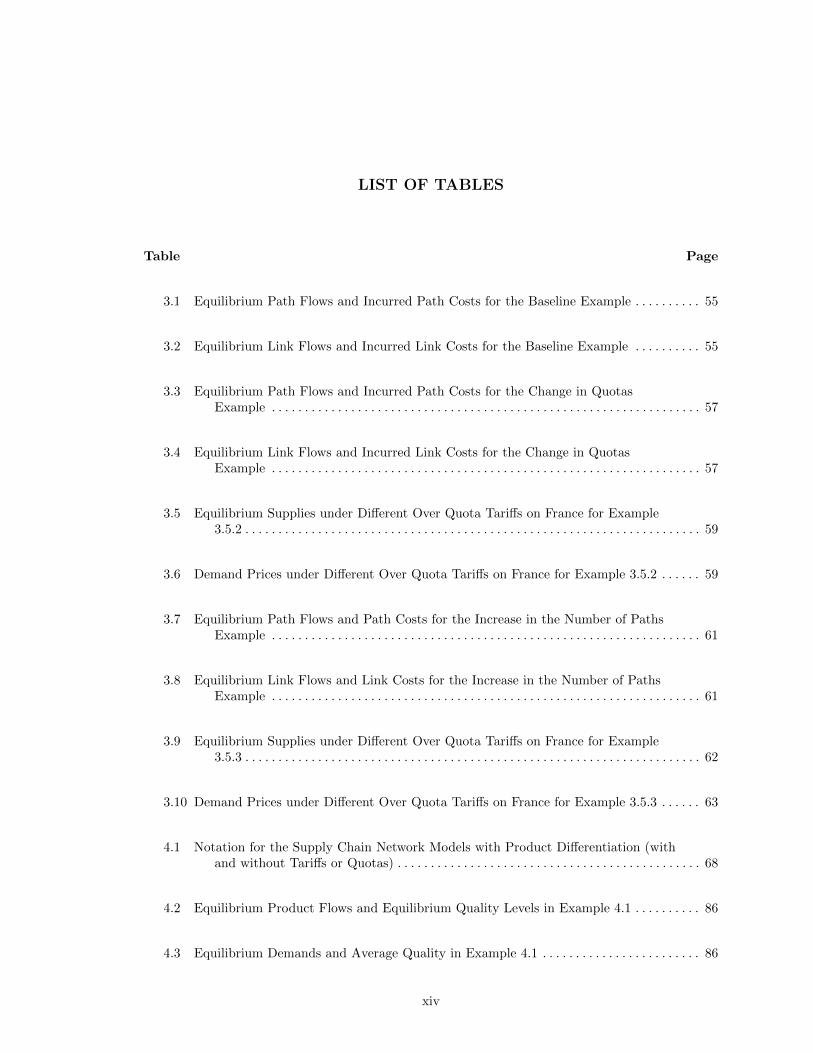
LIST OF TABLES
Table Page
3.1 Equilibrium Path Flows and Incurred Path Costs for the Baseline Example . . . . . . . . . . 55
3.2 Equilibrium Link Flows and Incurred Link Costs for the Baseline Example . . . . . . . . . . 55
3.3 Equilibrium Path Flows and Incurred Path Costs for the Change in QuotasExample . . . . . . . . . . . . . . . . . . . . . . . . . . . . . . . . . . . . . . . . . . . . . . . . . . . . . . . . . . . . . . . . . 57
3.4 Equilibrium Link Flows and Incurred Link Costs for the Change in QuotasExample . . . . . . . . . . . . . . . . . . . . . . . . . . . . . . . . . . . . . . . . . . . . . . . . . . . . . . . . . . . . . . . . . 57
3.5 Equilibrium Supplies under Different Over Quota Tariffs on France for Example3.5.2 . . . . . . . . . . . . . . . . . . . . . . . . . . . . . . . . . . . . . . . . . . . . . . . . . . . . . . . . . . . . . . . . . . . . . 59
3.6 Demand Prices under Different Over Quota Tariffs on France for Example 3.5.2 . . . . . . 59
3.7 Equilibrium Path Flows and Path Costs for the Increase in the Number of PathsExample . . . . . . . . . . . . . . . . . . . . . . . . . . . . . . . . . . . . . . . . . . . . . . . . . . . . . . . . . . . . . . . . . 61
3.8 Equilibrium Link Flows and Link Costs for the Increase in the Number of PathsExample . . . . . . . . . . . . . . . . . . . . . . . . . . . . . . . . . . . . . . . . . . . . . . . . . . . . . . . . . . . . . . . . . 61
3.9 Equilibrium Supplies under Different Over Quota Tariffs on France for Example3.5.3 . . . . . . . . . . . . . . . . . . . . . . . . . . . . . . . . . . . . . . . . . . . . . . . . . . . . . . . . . . . . . . . . . . . . . 62
3.10 Demand Prices under Different Over Quota Tariffs on France for Example 3.5.3 . . . . . . 63
4.1 Notation for the Supply Chain Network Models with Product Differentiation (withand without Tariffs or Quotas) . . . . . . . . . . . . . . . . . . . . . . . . . . . . . . . . . . . . . . . . . . . . . . 68
4.2 Equilibrium Product Flows and Equilibrium Quality Levels in Example 4.1 . . . . . . . . . . 86
4.3 Equilibrium Demands and Average Quality in Example 4.1 . . . . . . . . . . . . . . . . . . . . . . . . 86
xiv
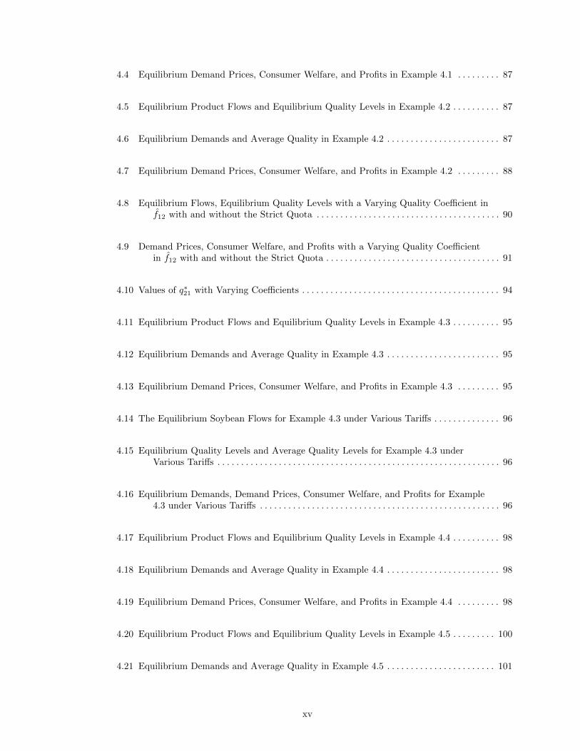
4.4 Equilibrium Demand Prices, Consumer Welfare, and Profits in Example 4.1 . . . . . . . . . 87
4.5 Equilibrium Product Flows and Equilibrium Quality Levels in Example 4.2 . . . . . . . . . . 87
4.6 Equilibrium Demands and Average Quality in Example 4.2 . . . . . . . . . . . . . . . . . . . . . . . . 87
4.7 Equilibrium Demand Prices, Consumer Welfare, and Profits in Example 4.2 . . . . . . . . . 88
4.8 Equilibrium Flows, Equilibrium Quality Levels with a Varying Quality Coefficient inf12 with and without the Strict Quota . . . . . . . . . . . . . . . . . . . . . . . . . . . . . . . . . . . . . . . 90
4.9 Demand Prices, Consumer Welfare, and Profits with a Varying Quality Coefficientin f12 with and without the Strict Quota . . . . . . . . . . . . . . . . . . . . . . . . . . . . . . . . . . . . . 91
4.10 Values of q∗21 with Varying Coefficients . . . . . . . . . . . . . . . . . . . . . . . . . . . . . . . . . . . . . . . . . . 94
4.11 Equilibrium Product Flows and Equilibrium Quality Levels in Example 4.3 . . . . . . . . . . 95
4.12 Equilibrium Demands and Average Quality in Example 4.3 . . . . . . . . . . . . . . . . . . . . . . . . 95
4.13 Equilibrium Demand Prices, Consumer Welfare, and Profits in Example 4.3 . . . . . . . . . 95
4.14 The Equilibrium Soybean Flows for Example 4.3 under Various Tariffs . . . . . . . . . . . . . . 96
4.15 Equilibrium Quality Levels and Average Quality Levels for Example 4.3 underVarious Tariffs . . . . . . . . . . . . . . . . . . . . . . . . . . . . . . . . . . . . . . . . . . . . . . . . . . . . . . . . . . . . 96
4.16 Equilibrium Demands, Demand Prices, Consumer Welfare, and Profits for Example4.3 under Various Tariffs . . . . . . . . . . . . . . . . . . . . . . . . . . . . . . . . . . . . . . . . . . . . . . . . . . . 96
4.17 Equilibrium Product Flows and Equilibrium Quality Levels in Example 4.4 . . . . . . . . . . 98
4.18 Equilibrium Demands and Average Quality in Example 4.4 . . . . . . . . . . . . . . . . . . . . . . . . 98
4.19 Equilibrium Demand Prices, Consumer Welfare, and Profits in Example 4.4 . . . . . . . . . 98
4.20 Equilibrium Product Flows and Equilibrium Quality Levels in Example 4.5 . . . . . . . . . 100
4.21 Equilibrium Demands and Average Quality in Example 4.5 . . . . . . . . . . . . . . . . . . . . . . . 101
xv
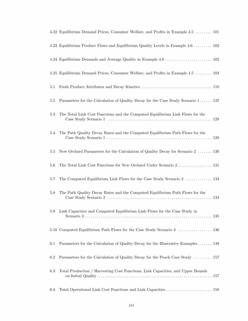
4.22 Equilibrium Demand Prices, Consumer Welfare, and Profits in Example 4.5 . . . . . . . . 101
4.23 Equilibrium Product Flows and Equilibrium Quality Levels in Example 4.6 . . . . . . . . . 102
4.24 Equilibrium Demands and Average Quality in Example 4.6 . . . . . . . . . . . . . . . . . . . . . . . 102
4.25 Equilibrium Demand Prices, Consumer Welfare, and Profits in Example 4.5 . . . . . . . . 103
5.1 Fresh Produce Attributes and Decay Kinetics . . . . . . . . . . . . . . . . . . . . . . . . . . . . . . . . . . . 110
5.2 Parameters for the Calculation of Quality Decay for the Case Study Scenario 1 . . . . . . 125
5.3 The Total Link Cost Functions and the Computed Equilibrium Link Flows for theCase Study Scenario 1 . . . . . . . . . . . . . . . . . . . . . . . . . . . . . . . . . . . . . . . . . . . . . . . . . . . . 128
5.4 The Path Quality Decay Rates and the Computed Equilibrium Path Flows for theCase Study Scenario 1 . . . . . . . . . . . . . . . . . . . . . . . . . . . . . . . . . . . . . . . . . . . . . . . . . . . . 128
5.5 New Orchard Parameters for the Calculation of Quality Decay for Scenario 2 . . . . . . . 130
5.6 The Total Link Cost Functions for New Orchard Under Scenario 2 . . . . . . . . . . . . . . . . . 131
5.7 The Computed Equilibrium Link Flows for the Case Study Scenario 2 . . . . . . . . . . . . . 133
5.8 The Path Quality Decay Rates and the Computed Equilibrium Path Flows for theCase Study Scenario 2 . . . . . . . . . . . . . . . . . . . . . . . . . . . . . . . . . . . . . . . . . . . . . . . . . . . . 134
5.9 Link Capacities and Computed Equilibrium Link Flows for the Case Study inScenario 3 . . . . . . . . . . . . . . . . . . . . . . . . . . . . . . . . . . . . . . . . . . . . . . . . . . . . . . . . . . . . . . . 135
5.10 Computed Equilibrium Path Flows for the Case Study Scenario 3 . . . . . . . . . . . . . . . . . 136
6.1 Parameters for the Calculation of Quality Decay for the Illustrative Examples . . . . . . . 149
6.2 Parameters for the Calculation of Quality Decay for the Peach Case Study . . . . . . . . . 157
6.3 Total Production / Harvesting Cost Functions, Link Capacities, and Upper Boundson Initial Quality . . . . . . . . . . . . . . . . . . . . . . . . . . . . . . . . . . . . . . . . . . . . . . . . . . . . . . . . . 157
6.4 Total Operational Link Cost Functions and Link Capacities . . . . . . . . . . . . . . . . . . . . . . . 158
xvi
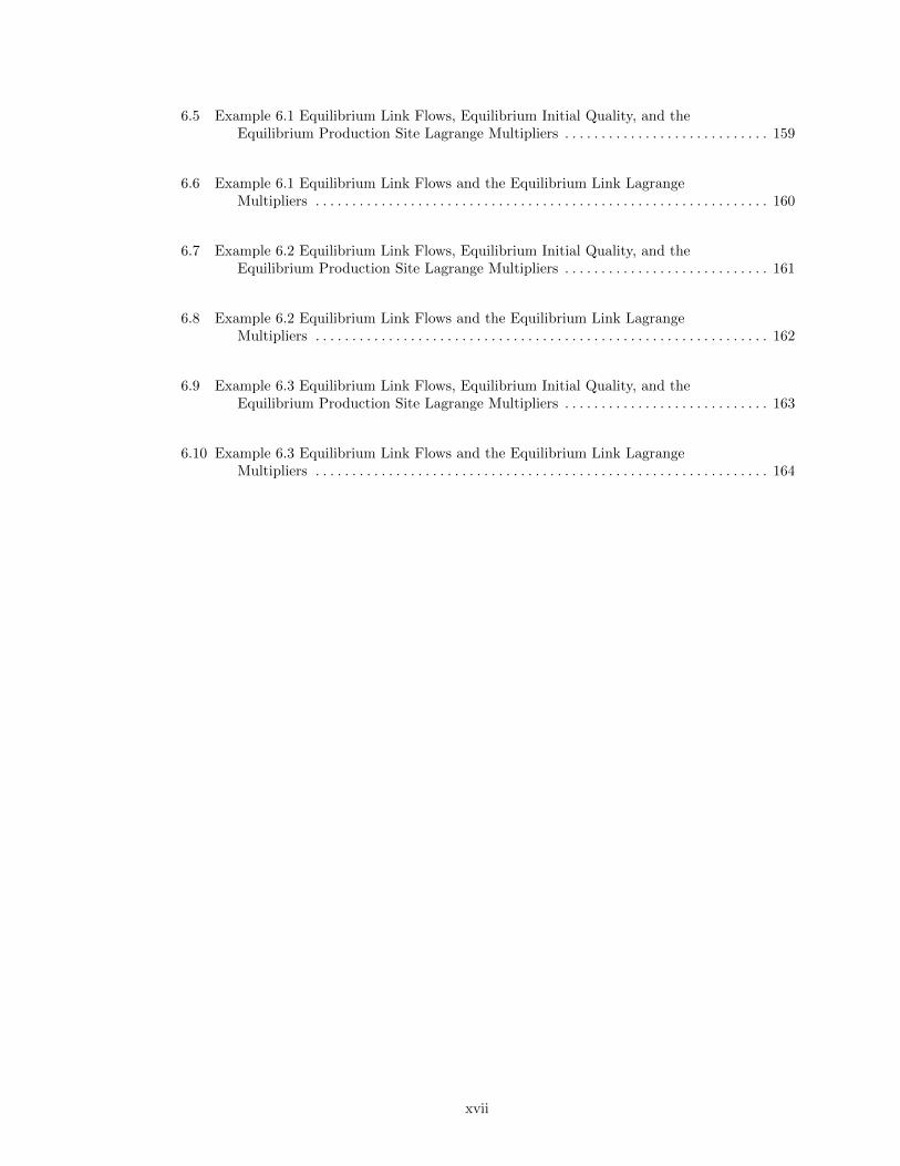
6.5 Example 6.1 Equilibrium Link Flows, Equilibrium Initial Quality, and theEquilibrium Production Site Lagrange Multipliers . . . . . . . . . . . . . . . . . . . . . . . . . . . . 159
6.6 Example 6.1 Equilibrium Link Flows and the Equilibrium Link LagrangeMultipliers . . . . . . . . . . . . . . . . . . . . . . . . . . . . . . . . . . . . . . . . . . . . . . . . . . . . . . . . . . . . . . 160
6.7 Example 6.2 Equilibrium Link Flows, Equilibrium Initial Quality, and theEquilibrium Production Site Lagrange Multipliers . . . . . . . . . . . . . . . . . . . . . . . . . . . . 161
6.8 Example 6.2 Equilibrium Link Flows and the Equilibrium Link LagrangeMultipliers . . . . . . . . . . . . . . . . . . . . . . . . . . . . . . . . . . . . . . . . . . . . . . . . . . . . . . . . . . . . . . 162
6.9 Example 6.3 Equilibrium Link Flows, Equilibrium Initial Quality, and theEquilibrium Production Site Lagrange Multipliers . . . . . . . . . . . . . . . . . . . . . . . . . . . . 163
6.10 Example 6.3 Equilibrium Link Flows and the Equilibrium Link LagrangeMultipliers . . . . . . . . . . . . . . . . . . . . . . . . . . . . . . . . . . . . . . . . . . . . . . . . . . . . . . . . . . . . . . 164
xvii
LIST OF FIGURES
Figure Page
3.1 An Example of a Multicountry, Multiple Supply Market and Multiple DemandMarket Spatial Price Network . . . . . . . . . . . . . . . . . . . . . . . . . . . . . . . . . . . . . . . . . . . . . . . 33
3.2 Network Topology for the Illustrative Example . . . . . . . . . . . . . . . . . . . . . . . . . . . . . . . . . . . 42
3.3 Spatial Network Structure of the Baseline Example . . . . . . . . . . . . . . . . . . . . . . . . . . . . . . . 52
3.4 Supply Chain Network Structure of the Increase in the Number of Paths Example . . . . . 60
4.1 The Differentiated Product Supply Chain Network Topology . . . . . . . . . . . . . . . . . . . . . . . 66
4.2 The Supply Chain Network Topology for the Illustrative Examples . . . . . . . . . . . . . . . . . 78
4.3 The Supply Chain Network Topology for Example 4.1 . . . . . . . . . . . . . . . . . . . . . . . . . . . . . 85
4.4 Equilibrium Product Shipments, Equilibrium Quality Levels, and Average QualityLevels as Quota Decreases for Example 4.2 . . . . . . . . . . . . . . . . . . . . . . . . . . . . . . . . . . . 92
4.5 Demands, Demand Prices, Profits, Consumer Welfare, and Lagrange Multipliers atEquilibrium as Quota Decreases for Example 4.2 . . . . . . . . . . . . . . . . . . . . . . . . . . . . . . 93
4.6 The Supply Chain Network Topology for Example 4.4 . . . . . . . . . . . . . . . . . . . . . . . . . . . . . 97
4.7 The Supply Chain Network Topology for Example 4.5 . . . . . . . . . . . . . . . . . . . . . . . . . . . . 100
5.1 The Supply Chain Network Topology of the Farmer’s Market Competitive FreshProduce Problem . . . . . . . . . . . . . . . . . . . . . . . . . . . . . . . . . . . . . . . . . . . . . . . . . . . . . . . . . 113
5.2 The Supply Chain Network Topology for the Apple Farmers’ Markets Case Study –Scenario 1 . . . . . . . . . . . . . . . . . . . . . . . . . . . . . . . . . . . . . . . . . . . . . . . . . . . . . . . . . . . . . . . 124
xviii
5.3 The Supply Chain Network Topology for the Apple Farmers’ Markets Case Study -Scenario 2 . . . . . . . . . . . . . . . . . . . . . . . . . . . . . . . . . . . . . . . . . . . . . . . . . . . . . . . . . . . . . . . 130
6.1 The Fresh Produce Supply Chain Network Topology with Quality Deterioration . . . . . 141
6.2 Supply Chain Network Topology for the Illustrative Examples . . . . . . . . . . . . . . . . . . . . . . . . . 148
6.3 Supply Chain Network Topology of the Case Study Focusing on Peaches . . . . . . . . . . . 156
xix
CHAPTER 1
INTRODUCTION AND RESEARCH MOTIVATION
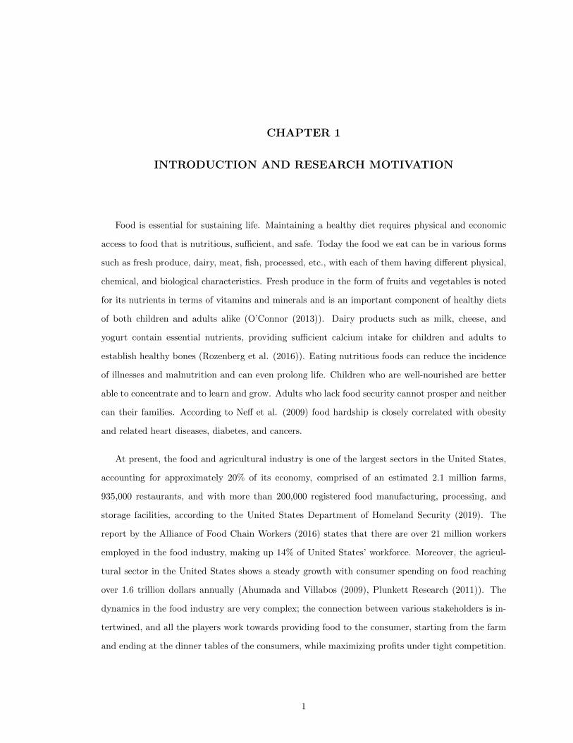
Food is essential for sustaining life. Maintaining a healthy diet requires physical and economic
access to food that is nutritious, sufficient, and safe. Today the food we eat can be in various forms
such as fresh produce, dairy, meat, fish, processed, etc., with each of them having different physical,
chemical, and biological characteristics. Fresh produce in the form of fruits and vegetables is noted
for its nutrients in terms of vitamins and minerals and is an important component of healthy diets
of both children and adults alike (O’Connor (2013)). Dairy products such as milk, cheese, and
yogurt contain essential nutrients, providing sufficient calcium intake for children and adults to
establish healthy bones (Rozenberg et al. (2016)). Eating nutritious foods can reduce the incidence
of illnesses and malnutrition and can even prolong life. Children who are well-nourished are better
able to concentrate and to learn and grow. Adults who lack food security cannot prosper and neither
can their families. According to Neff et al. (2009) food hardship is closely correlated with obesity
and related heart diseases, diabetes, and cancers.
At present, the food and agricultural industry is one of the largest sectors in the United States,
accounting for approximately 20% of its economy, comprised of an estimated 2.1 million farms,
935,000 restaurants, and with more than 200,000 registered food manufacturing, processing, and
storage facilities, according to the United States Department of Homeland Security (2019). The
report by the Alliance of Food Chain Workers (2016) states that there are over 21 million workers
employed in the food industry, making up 14% of United States’ workforce. Moreover, the agricul-
tural sector in the United States shows a steady growth with consumer spending on food reaching
over 1.6 trillion dollars annually (Ahumada and Villabos (2009), Plunkett Research (2011)). The
dynamics in the food industry are very complex; the connection between various stakeholders is in-
tertwined, and all the players work towards providing food to the consumer, starting from the farm
and ending at the dinner tables of the consumers, while maximizing profits under tight competition.
1
The system for creating and sustaining the connection between the farm and the consumer is called
a food supply chain network.
Food supply chains are very intricate local, regional or global networks, creating pathways from
farms to consumers, encompassing production, processing, storage, and distribution (Yu and Nagur-
ney (2012)). In general, food or agricultural supply chains are divided into two main types: per-
ishable food supply chains and non-perishable food supply chains. Perishable foods include fresh
produce, in the form of fruits and vegetables, dairy, meat, and fish. Fresh produce is seen as one
of the most dynamic branches in the food sector with an annual consumption value of 100 billion
products (Ahumada and Villabos (2009)). Population growth, coupled with the emphasis on the
benefits of healthier diets, has lead to an increase in the demand for fresh produce. The Department
of Agriculture (USDA) (2011) claims that the increase in the fresh produce consumption is higher
than it is for traditional crops such as wheat and other grains.
In the United States, the growth in demand, and the increased expectations of the consumers for
year-around availability of fresh produce, has spurred food supply chains to evolve into more sophis-
ticated systems involving overseas production in different countries including Mexico, Argentina,
Chile, and even Canada. Due to seasonality, most of the fresh produce that is sold in the grocery
stores in the northeast of the United States is imported from other countries, or grown domestically
in a state such as California or Florida (Cook (2002)). It is reported that two thirds of United States’
vegetable imports come from Mexico, and most of the remainder arrives from Canada (Cook (2002)).
Hence, the interactions between the demand and supply of food are no longer limited to a nation or
a region, but have grown into a larger cross-border operation, including complex relationships and
long distances (Van der Vorst (2000)).
There are multiple challenges related to food supply chain management, and it is not very
straight-forward to conceive a general rule of thumb for managing food supply chains, since each
and every food supply chain incorporates unique challenges pertinent to the specific product and
process characteristics (Rong, Akkerman, and Grunow (2011)). One of the complexities of managing
food supply chains ensues from the perishable nature of the product, making them distinct from
other product supply chains (Yu and Nagurney (2012)).
Another feature associated with food supply chains is the issue of providing good quality fresh
produce. Quality of perishable food products changes continuously throughout the supply chain
from the farm to the fork. The quality change of food products depends on the environmental
2
conditions of the supply chain activities. Labuza (1982) states that keeping the quality of the per-
ishable food products at the acceptable limits is vital for measuring the performance of food supply
chains. Understanding the chemistry of quality decay, especially for fresh produce, is imperative for
maintaining a better quality of the food product. In order to address this real-world supply chain
issue, more explicit quality decay models, capturing time and temperature, in food supply chains
are essential.
One of the other issues that is worth investigating in supply chain networks, including food supply
chains, is the impact of trade policies. The increased amount of commodity flow between countries
through supply chains has intensified the role of trade policies on nations’ economies. The surge
of globalization and the surge of global trade have induced governments to impose trade barriers
in the form of tariffs, quotas, and their combination, tariff-rate quotas (TRQs), to protect their
domestic markets from foreign competition. Historically, economists and policy makers believed
that an increased trade volume can make a nation prosper, whereas trade restrictions may hurt its
economy. Today, this belief is frequently questioned by government leaders, economists, and public
officials. Hence, I attempt to provide a rigorous mathematical framework that incorporates the trade
instruments used in practice today, especially in the agricultural industry, to illustrate and quantify
the impacts, which, in turn, can provide valuable managerial insights for policy makers.
Additionally, considering the importance of trade instruments, and the effects of quality on supply
chain network modeling, it is essential to explore the relationship between the two phenomena. This
area of research, coupled with discussions on minimum quality standards, has also been garnering
attention and has been the subject of debates (cf. Lutz (2005) and Nagurney and Li (2016)). In
this dissertation, I also investigate quality, along with trade issues in perishable food supply chain
networks.
In subsequent sections of this chapter of the dissertation I provide my motivation for studying
trade and policy instruments, and product quality in perishable supply chain networks. I also provide
a literature review, an outline of the dissertation, and contributions.
1.1. Trade and Policy Instruments
Trade allows countries to advance in their economic activities through the exchange of goods
and services that they have an advantage of in terms of production cost (Smith (1887)). With this
simple and very fundamental idea, nations engage in trade to increase their productivity levels,
3
employment rates, and general economic welfare. Today, products as diverse as fresh produce
and other agricultural and food products such as meat, fish and seafood, cereals, including rice
and wheat, and dairy products, to steel and aluminum, and a variety of other commodities, are
transported across national boundaries to points of demand to satisfy the needs of the consumers.
The competition among nations, however, has become more relentless with the increase in global
trade volumes, and opportunities in emerging markets. The advancements in technology and com-
munication in the developed world created better and more efficient global supply chains, encouraged
investments in the emerging markets, which, in turn, constructed a more complex and intertwined
state of global trade. The spread of international trade has increased over time, fueled by globaliza-
tion, reduced trade barriers, liberalized trade policies, overseas production, improved communication,
and investments on technology.
A more transparent and open world economy, created by advancements in globalization, grants
more opportunities for developing nations. It is reported by the World Trade Organization (WTO)
that the share of developing nations in global trade has risen from a third to a half, since 1980
(WTO Report (2014)). Furthermore, China, being the top exporter today, was ranked 32nd thirty
years ago (WTO Report (2014)). However, there is still an ongoing discussion about whether a
more open and lenient trade environment contributes to the growth of the economy. According to
a White House report in the United States in 2009, engagements on trade created more production,
and also contributed to an increase in the standard of living in the United States.
Given the importance of global trade for producers and consumers alike, governments, often turn
to trade policies ranging from tariffs and quotas, and their combination, in the form of tariff-rate
quotas (TRQs), in order to reduce the impact of competitive foreign firms on their demand markets
and to protect their less competitive domestic firms. Trade instruments can be seen as a type of tax
that is imposed on goods at the time of import. For example, a tariff-rate quota (TRQ) is a two-
tiered tariff, in which a lower in-quota tariff is applied to the units of imports until a quota is attained
and then a higher over-quota tariff is applied to all subsequent imports (World Trade Organization
(2004)). In general, tougher trade policies on imports may bolster the domestic industries of the
expense of generating higher prices for domestic consumers. Skully (2001) states that the Uruguay
Round in 1996 created more than 1,300 new TRQs. Furthermore, the World Trade Organization
members currently have a combined total of 1,425 TRQ commitments.
4
In the present economic and political climate, tariffs, as well as tariff-rate quotas, are garnering
prominent attention in the news on world trade with even washing machines in the United States
being subject to tariff-rate quotas (cf. Office of the United States Trade Representative (2018)).
The imposition of tariffs by certain countries, including the United States, is, in turn, leading to
retaliation by other nations, such as China, European Union, Mexico, and Canada, with ramifications
across multiple supply chains (cf. Watson (2018)). For example, in March 2018, the United States
government imposed a 25 percent tariff on imported steel and a 10 percent tariff on imported
aluminum (cf. Hodge (2018)). These exchanges between the world’s two largest economies were seen
as the beginning of the largest trade war in the economic history of trade. In fact, economists argue
that the on-going trade war with China and the latest round of proposed tariffs on Chinese goods
would eventually hurt the American consumers (cf. Tankersley (2018)). It was reported in 2020 that
the American manufacturing activity was facing a decline, damaged by the trade war between US
and China, while the dollar was steadily strong against other currencies, making American goods
more expensive (cf. Swanson and Smialek (2020)). Moreover, the recent developments in the global
political environment could result in the separation of world’s famous conjoined twins, the United
States and China, induced by the decoupling of global supply chains between the world’s two largest
economies (cf. Mistreanu (2019)).
While the major financial impacts on nations’ economies are generated by the trade wars between
the United States and China, there are other players in the most popular trade game of 2000s. It was
announced in 2020 that the United States could impose 100 percent tariffs on European wine, Irish
whiskey, and waffles due to European Union’s financial support for the European aerospace company
Airbus, a competitor of American aerospace company Boeing (cf. Lefcourt (2020), Tankersley
(2019)).
As international trade continues to be a very crucial part of the global social, political, and
financial environments, there are very few mathematical models for the evaluation of the impacts
of tariffs, quotas, and TRQs. The development of rigorous mathematical models that can capture
trade policies used in practice today and that are computable, providing both equilibrium supply
market prices and demand market prices, as well as product flows, is critical. Such models should be
sufficiently general to be able to handle multiple supply and demand markets in different countries,
trade flows on general networks, as well as nonlinear cost and price functions that are also asymmetric
and flow-dependent. With this motivation, I model TRQs, tariffs, and quotas in a supply chain
equilibrium network framework, and provide a case study on dairy products in Chapter 3.
5
Trade and policy instruments may also generate implications on a micro level, that is, the quality
of export products can change by imposition of stricter trade policies. Therefore, studying the
relevance of quality of the products with trade instruments in the context of global supply chains,
including food supply chains, is essential for having an understanding on the impacts of global trade.
This motivation creates a foundation for the mathematical model that I present in Chapter 4, while
providing a case study on soybeans.
1.2. Perishable Food Supply Chains
The transformation of global food supply chains since the early 1900s has been nothing short
of remarkable. As reported in Martinez et al. (2010), in the early 1900s, much of the food bought
and consumed in the United States was grown locally and about 40% of Americans resided on
farms, whereas in 2000 only 1% did (cf. Pirog (2009)). Consumers over a century ago obtained
information as to the quality of the foods through direct contact with farmers. Except for various
food preservation activities, few foods were processed or packaged, and fresh produce, fish, and
dairy products usually traveled less than 24 hours to market (see Giovannucci, Barham, and Pirog
(2010)). According to a report by DeWeerdt (2016), in 1993, a Swedish researcher determined that
the ingredients of a typical Swedish breakfast consisting of an apple, bread, butter, cheese, coffee,
cream, orange juice, and sugar, had traveled a distance equal to the circumference of our planet
before reaching the consumer.
The basic difference between food supply chains and other supply chains, and this is espe-
cially characteristic of fresh produce, is the continuous and significant change in the quality of food
products throughout the entire supply chain from the points of production/harvesting to points
of demand/consumption (see Sloof, Tijskens, and Wilkinson (1996), Van der Vorst (2000), Lowe
and Preckel (2004), Ahumada and Villalobos (2009), Blackburn and Scudder (2009), Akkerman,
Farahani, Grunow (2010), Aiello, La Scalia, and Micale (2012)).
In the next subsection, I extend the discussion on perishable food supply chains by providing
more information on the ways of capturing quality of food products.
1.2.1 Quality of Food Products
The quality of food products is decreasing with time, even with the use of advanced facilities
and under the best processing, handling, storage, and shipment conditions (Sloof, Tijskens, and
Wilkinson (1996) and Zhang, Habenicht, and Spieß (2003)). The network topology of a fresh produce
6
supply chain and, in particular, the length of a path in terms of time from an origin node to a
destination node can significantly influence the quality of the fresh produce that consumers purchase
and consume.
Knowledgeable modern consumers are increasingly demanding high quality in their food prod-
ucts, including fresh produce, and, yet, they may be unaware of the great distances the food has
traveled through intricate supply chains and the length of time from the initial production or “pick-
ing” of the fruits and vegetables to the ultimate delivery. Moreover, consumers, faced with informa-
tion asymmetry, may not know how long the food may have been lying on the grocers’ and retailers’
shelves, even once delivered and unpacked. The great distances traveled create issues in terms of
quality since fresh produce is perishable (see Nahmias (2011) and Nagurney et al. (2013)).
In order to capture quality degradation associated with fresh produce in a supply chain one
must be aware of the various supply chain network economic activities such as production, storage,
transportation, etc., as well as the duration and temperature associated with these activities. It has
been discovered that the quality of fresh produce can be determined scientifically using chemical
formulae, which include both time and temperature (cf. Labuza (1982), Taoukis and Labuza (1989),
Tijskens and Polderdijk (1996), Rong, Akkerman, and Grunow (2011)). For example, in terms of
kinetics (cf. Labuza (1982)), the quality degradation of food such as meat and fish follows first
order reactions whereas that of many fresh fruits and vegetables follows zero-order reactions with
the order of the reaction corresponding to the power of the differential equation for quality. Hence,
studying and integrating quality decay into food supply chain networks can be seen as the pillars
for my work in Chapters 5 and 6 of this dissertation.
I now review the relevant literature on: tariffs and quotas from a network equilibrium point of
view, the relevance of product quality on the network equilibrium models with tariffs and quotas,
and the modeling of fresh produce supply chain networks with the incorporation of fresh produce
quality.
1.3. Literature Review
Through this dissertation, I contribute to the modeling and analysis of supply chain network
equilibrium modeling, especially to that of perishable food supply chain networks. I contribute
significantly to the literature on variational inequalities, game theory, and supply chain network
equilibrium modeling by being methodologically relevant to the application and solution of such
7
problems. The results obtained from analyzing the mathematical models based on simulated case
studies provide valuable insights and can inform policy makers.
Thus, this section discusses the relevant literature on several topics covered in this dissertation.
1.3.1 Perfectly and Imperfectly Competitive Models for Agricultural Trade Problems
To-date, the modeling of trade problems that include multiple producers in different countries as
well as multiple demand markets while using supply chain network equilibrium modeling framework
is limited. The studies in this area mostly consider perfect competition, in which all firms are
price takers, and produce a homogeneous product. As an example of perfectly competitive models,
spatial price equilibrium (SPE) models have attained prominence in the modeling, analysis, and
solution of a wide spectrum of commodity trade problems. However, in many industrial sectors,
the more appropriate framework for modeling is that of imperfect competition, such as oligopolistic
competition, in which the market is dominated by few firms, and the decisions of one firm influencing
the decisions of other firms, vice versa. In this subsection, I present a review on perfectly competitive
models with a focus on SPE models, and also oligopolistic models for commodity trade problems.
1.3.1.1 Spatial Price Equilibrium Models
SPE problems are perfectly competitive models, in that therein it is assumed that there are
numerous producers, and such models date to Samuelson (1952) and Takayama and Judge (1964,
1971). The need to develop extensions, over and above the original SPE models that were reformu-
lated and solved using optimization approaches, especially quadratic programming ones, has also
spearheaded advances through the use of methodologies such as complementarity theory as well as
variational inequality theory.
Harker (1985) points out that SPE problems are appealing for scholars; firstly, for their appli-
cation to energy markets, steel markets etc., leading researchers to reexamine the structure of the
model, and, secondly, the availability of new mathematical methods and algorithms for achieving
solutions of the problem. Asmuth, Eaves, and Peterson (1979) reformulate the SPE problem as
a complementarity problem, and solve for an equilibrium on affine networks with Lemke’s algo-
rithm. Florian and Los (1982) propose a newer and more general formulation of SPE, providing
more efficient and simpler algorithms. The authors present formulations that can be applied to
general transportation networks, allowing multiple commodities on the condition of an equivalent
optimization problem reformulation.
8
SPE models, due to their practical applications in agricultural and energy and mineral markets,
have incorporated trade policies and have been constructed using variational inequality. Nagurney,
Nicholson, and Bishop (1996a,b) develop an SPE model with discriminatory ad valorem tariffs. The
authors provide a solution method that includes parallel programming, in which the main problem
is broken down into simple subproblems, each of which is solved simultaneously. Nagurney and
Zhao (1993) introduce competitive spatial market models with direct demand functions. The policy
interventions in the form of price controls is permitted in their modeling framework. Nagurney,
Thore, and Pan (1996) illustrate a spatial market policy modeling with goal targets, in which they
use variational inequality theory for the formulation, qualitive analysis, and computation.
Complementarity theory is also widely used for the modeling of quotas and tariff schemes.
Rutherford (1995) introduces new features using GAMS modeling, and solves nonlinear complemen-
tarity problems applied to various economic models. Moreover, Nolte (2008) constructs a spatial
price equilibrium model of the world sugar market with various trade instruments. The authors use
the mixed complementarity problem to program the SPE model, and use GAMS for the computa-
tional study. On the other hand, Grant, Hertel, and Rutherford (2009) propose a partial equilibrium
model of the United States’ dairy market to analyze the options of liberalization on various trade
instruments including tariff quotas, and quota expansions. They conduct simulation analysis to eval-
uate different scenarios with various trade instruments. Recently, Johnston and van Kooten (2017)
develop a spatial price equilibrium model to analyze the impacts of softwood lumber trade sanc-
tions between Canada and the United States. The authors use a mixed complementarity problem
formulated to solve a 21-region, global trade model.
1.3.1.2 Oligopolistic Models
Another framework for modeling agricultural trade is that of oligopolistic competition. The
connection between spatial price equilibrium models and oligopolies are shown in the paper by
Dafermos and Nagurney (1987), in which the authors present a general spatial price equilibrium
model, and solve for the corresponding Cournot (1838) oligopoly equilibrium using variational in-
equality theory. In addition, the authors conduct a sensitivity analysis for the general spatial price
equilibrium problem in their earlier work (Dafermos and Nagurney (1984)). Oligopolistic models
can be very appropriate for the modeling of agricultural trade problems, since the number of firms,
that is, “players” in the game may not be very large. As noted by Guyomard et al. (2005), the
world banana market is dominated by a small number of firms and, hence, this raises the impor-
9
tance of also addressing imperfect competition. Nagurney, Besik, and Nagurney (2019) develop an
global supply chain network model where firms engage in oligopolistic competition to maximize their
profits in the presence of trade policy instruments in the form of tariff-rate quotas. The authors
allow firms to have production sites in different countries, determining how much of the product to
manufacture/produce at these production sites, along with the distribution of the product flows to
the demand markets, also located in multiple countries. In Chapters 4,5, and 6 of this dissertation,
I present supply chain network models with firms competing in an oligopolistic manner.
The literature is very limited in terms of oligopoly models on trade problems. For example, Shono
(2001) relaxes the assumption of perfect competition, and incorporates TRQs. The author assumes
that all countries behave in the same oligopolistic manner. Moreover, Maeda, Suzuki, and Kaiser
(2001, 2005) consider oligopolistic competition and TRQs with a single producer in each country and
that it is faced with a separable cost function. The authors also assume that the demand function
in each country is also separable, that is, the demand for a product in a country only depends on
the price in that country.
For additional supply chain network equilibrium models with oligopolies the interested reader
is encouraged to see Nagurney and Matsypura (2005), Zhang (2006), Daniele (2010), Qiang et al.
(2013), Yu and Nagurney (2013), Li and Nagurney (2017), Nagurney, Yu, and Besik (2017), and
Saberi (2018).
In the next subsection, I provide a literature review on product quality in perishable food supply
chains.
1.3.2 Product Quality in Perishable Food Supply Chains
The literature on food supply chains is growing, given the great interest in this topic. The
early contributions focused on perishability and, in particular, on inventory management (see Ghare
and Schrader (1963), Nahmias (1982, 2011) and Silver, Pyke, and Peterson (1998) for detailed
reviews). More recently, some studies have proposed integrating more than a single supply chain
network activity (see, e.g., Zhang, Habenicht, and Spieß (2003), Widodo et al. (2006), Ahumada and
Villalobos (2011), and Kopanos, Puigjaner, and Georgiadis (2012)) and also have emphasized the
need to bring greater realism to the underlying economics and competition (cf. Yu and Nagurney
(2013)). Van der Vorst (2006) noted that it is essential to analyze food supply chains within the
context of the full complexity of their network structure. Monteiro (2007), further, postulated that
10
network economics (cf. Nagurney (1999)) provides a powerful framework in which the structure of the
supply chain can be graphically captured and analyzed, and studied the traceability in food supply
chains theoretically. Additional modeling and methodological contributions in the food supply chain
and quality domain have been made by Blackburn and Scudder (2009) and by Rong, Akkerman,
and Grunow (2011). For approaches to the quantification of quality in supply chain networks of
manufactured products, including durable goods, we refer the interested reader to the book by
Nagurney and Li (2016) and the references therein. For a recent book on perishable product supply
chains with a variety of applications, see Nagurney et al. (2013).
Quality can be defined in multiple dimensions such as physical, emotional, and even philosophical.
Therefore, it is not easy to find a proper global definition of quality which is valid for every type
of industry and consumer. Reeves and Beednar (1994) present a good discussion on the evolution
of quality definitions. Nagurney and Li (2014) investigate minimum quality standards in a spatial
price equilibrium model and also consider information asymmetry. Nagurney and Li (2016) present
a plethora of competitive supply chain network models with a focus on quality, where quality is
defined as conformance to specifications as in manufactured products. Nagurney et al. (2013), in
turn, focus on perishable product supply chains. Murdoch, Marsden, and Banks (2000) also present
a valuable discussion on the connection between quality and nature, especially in the food sector,
from the perspective of social sciences. However, there are more specific definitions of quality in the
literature that are construed specifically for the food sector.
Various authors have emphasized the change in quality of food products in the supply chain until
the final points of demand (see Sloof, Tijskens, and Wilkinson (1996), Van der Vorst (2000), Lowe and
Preckel (2004), Ahumada and Villalobos (2009, 2011), Blackburn and Scudder (2009), Akkerman,
Farahani, and Grunow (2010), and Aiello, La Scalia, and Micale (2012), Yu and Nagurney (2013)).
Amorim, Costa, and Almada-Lobo (2014) utilize demand functions that depend on product quality
and also price and then construct demands for different products based on age. They propose
deterministic and stochastic production planning models that capture consumers’ desire for fresher
products. Liu, Zhang, and Tang (2015) also utilize demand functions that depend on price and
quality but they depend continuously on time. The authors determine the dynamic pricing and
investment strategies to reduce the deterioration rate of the quality for perishable foods.
11
1.3.3 Modeling of Quality in the Presence of Tariffs and Quotas
The state-of-the-art literature pertinent to the supply chain network equilibrium modeling of
tariffs and quotas with the incorporation of product quality is not advanced. Much of the modeling
research in this domain that includes the quality of products produced and traded has appeared in
the economics literature and has focused, in terms of theoretical results, on either a monopoly or
perfect competition (Falvey (1979), Krishna (1987)) or on a duopoly (Das and Donnenfeld (1989),
Herguera, Kujal, and Petrakis (2000)). As for oligopolistic competition, researchers have, typically,
assumed exogenously fixed product qualities or homogeneous goods (Leland (1979), Shapiro (1983),
Deneckere, Kovenock, and Sohn (2000)), whereas it is clear that quality can be a strategic variable
in firms’ decision-making and also in terms of consumers differentiating among the firms. There
have also been empirical studies conducted to assess the interrelationships between a spectrum of
trade policies and product quality as in cheese (cf. Macieira and Grant (2014)), the steel industry
(Boorstein and Feenstra (1991)), the footwear industry (Aw and Roberts (1986)), and the automo-
bile industry (cf. Feenstra (1988), Goldberg (1993)). Nevertheless, the construction of a general
differentiated supply chain network model with product quality and trade policies in the form of
tariffs, quotas, and also minimum quality standards merits attention, especially since the theoretical
literature has been limited in terms of the number of firms considered, as well as the number of
demand markets, and has not included general transportation cost functions that include quality.
1.4. Dissertation Overview
The dissertation consists of seven chapters with the first chapter dealing with the research mo-
tivation and literature review. In Chapter 2, I recall the methodologies that are utilized in this
dissertation, mainly variational inequality theory (Nagurney (1999)) and its relation to game theory
(Nash (1950,1951)). In the next subsections, I present the contributions in Chapters 3 through 6.
1.4.1 Contributions in Chapter 3
In Chapter 3 of this dissertation, I provide a unified variational inequality framework for the
modeling, analysis, and computation of solutions to a general spatial network equilibrium problem
with multiple countries and regions in each country on both the production and on the consumption
sides, as well as multiple routes joining the supply markets with the demand markets, in the presence
of two-tiered tariffs in the form of tariff-rate quotas.
12
I extend the literature on spatial price equilibrium models by incorporating various policy inter-
ventions such as tariff-rate quotas. Since different supply and demand markets may have, respec-
tively, distinct supply and demand price functions, and trade policies such as tariff-rate quotas can
impose quotas over multiple countries, I believe that having a greater level of detail is meaningful.
Furthermore, rather than assuming only a single path (essentially a link) between a pair of supply
and demand market nodes, I allow for multiple paths, each of which is not limited to the same num-
ber of links. Different supply markets in a given country may have distinct transport mode options
to demand markets in the same or other countries, and, therefore, such options can be represented
as paths on the general network, with associated costs. I focus on tariff-rate quotas (TRQs) since
they have been deemed challenging to formulate and only stylized examples have been reported in
an SPE framework (cf. Bishop et al. (2001)). I believe that the modeling of TRQs just by itself
adds a great contribution to the literature.
In addition, I construct variants of the general spatial price network equilibrium model with tariff-
rate quotas, to demonstrate how the latter can be easily adapted to handle unit tariffs, ad valorem
tariffs, and/or strict quotas. I also note that, through the use of multiple paths, the evaluation of
avenues for transshipment, as a means to avoid tariffs, a topic that has garnered a lot of attention
in the popular press recently (cf. Bradshear (2018)), is made possible. Moreover, my framework
allows for the investigation of the impacts of TRQs on domestic markets, on both producers and
consumers alike, that are imposed on non-domestic markets.
Another contribution of this chapter emerges from the results analyzed in the computational
study section. I provide illustrative examples as well as a case study consisting of larger numerical
examples for which the equilibrium path flows, and link flows, as well as the equilibrium quota rents,
and the supply and demand markets prices, and path costs, are reported. The case study focuses
on the dairy industry and a tariff-rate quota imposed on the US on cheese from France. Sensitivity
analysis demonstrates the impacts on production outputs (both US domestic and imports from
France) of a tightening of the imposed quota as well as increases in the over tariff-rate. The case
study includes adding routes between producing and consuming regions in different countries. The
results show that tariff-rate quotas may protect domestic producers, but at the expense of the
consumers. On the other hand, adding competitive alternative transportation routes may help both
domestic producers and exporters as well as consumers. These results bring great value to the supply
chain network and game theory literature as well as to the literature on trade policy, since I provide
13
insights to policy makers for their decision making on international trade policies. Chapter 3 of this
dissertation is based on the paper by Nagurney, Besik, and Dong (2019).
1.4.2 Contributions in Chapter 4
In Chapter 4, I extend the mathematical model constructed in Chapter 3 by incorporating
quality. I add to the supply chain network, game theory and trade policy literature by developing
an oligopolistic supply chain network equilibrium model with differentiated products in which firms
have multiple production sites and multiple possible demand markets, and compete in product
quantities and product quality, subject to minimum quality standards, along with upper bounds
on quality. The model is then extended to include trade policy instruments in the form of a strict
quota or a tariff. I identify the governing equilibrium conditions, noting that the strict quota model
is characterized by a Generalized Nash Equilibrium (GNE), rather than a Nash Equilibrium. Under
a strict quota, both the utility functions of the competing firms, as well as their feasible sets, will
depend on the strategic variables of not only the particular firm, but also on the strategies of the
others. Hence, I define a Generalized Nash Equilibrium. The GNE problem dates to Debreu (1952)
and Arrow and Debreu (1954), and for background on the GNE problem, I refer the interested reader
to von Heusinger (2009) and the recent review by Fischer, Herrich, and Schonefeld (2014). Moreover,
I utilize the concept of a Variational Equilibrium (cf. Facchinei and Kanzow (2010), Kulkarni and
Shanbhag (2012)) which is a specific kind of GNE to construct the variational inequality formulation.
It is worthwhile to add that this is the first time that such concepts have been utilized in competitive
supply chain network models with quality with or without trade policy instruments.
Subsequently, I introduce a differentiated product supply chain network equilibrium model with
a tariff and prove that this model coincides with the model with a strict quota where the Lagrange
multiplier associated with the latter, if the strict quota constraint is tight, is precisely the imposed
tariff. In the economics literature, Bhagwati (1965) considered perfect competition (whereas we
consider imperfect competition) and demonstrated that the tariff-quota equivalence occurs when
such competition prevails in all markets. Fung (1989), in turn, considered a stylized oligopoly
consisting of two countries with a single firm in each country and Cournot-Nash competition and
also found an equivalence.
Moreover, I demonstrate that, the underlying equilibrium conditions for all three models can be
formulated and analyzed as an appropriate variational inequality problem, for which an effective
14
computational scheme is also provided, which yields closed form expressions for the variables in each
of the two steps of the procedure.
I also provide constructs for quantifying consumer welfare in the presence or absence of tariffs
or quotas in differentiated product supply chain networks with quality. Through simple illustrative
examples, I show that the imposition of a tariff or quota may adversely affect both the quality of
products as well as the consumer welfare. I contribute significantly to the existing literature on the
supply chain networks, and game theory. This chapter is based on the paper by Nagurney, Besik,
and Li (2019).
1.4.3 Contributions in Chapter 5
In Chapter 5, I analyze fresh produce quality in a more detailed fashion in which I present
a modeling and algorithmic framework for competitive farmers’ markets. This work makes sev-
eral contributions to the existing literature on competitive perishable supply chains. The model is
network-based and the farmers engage in Cournot competition over space and time. The govern-
ing Nash equilibrium conditions are formulated as a variational inequality problem. The novelty
of the framework lies in that the quality of the fresh produce product is captured as the produce
propagates in the supply chain over space and time with the consumers at the markets responding
both to the price and the quality of the fresh produce. Both uncapacitated and capacitated versions
of the model are presented. The latter can capture limitations in supply due to harvest problems
or damage during the growing season, limitations in transport and storage capabilities, and/or la-
bor for harvesting and processing. The game theory model can address questions of farmers as to
which farmers’ markets they should serve; what the impact of a new competitor may be at one or
more markets in terms of profits, as well as the effects of capacity disruptions (or enhancements) in
their individual and others’ short supply chains. In addition, the model can ascertain the impacts
of changes in link parameters that capture quality. Policy makers, in turn, can also obtain useful
information as to the impacts of a greater number or fewer farms represented at various markets
and how reducing quality decay can affect farmers’ profits.
One of my other contributions to the literature arises from handling the quality deterioration
of fresh produce along supply chains. With the intent of modeling the quality of fresh produce
products, I provide some preliminaries, focusing on the quality differential equations, which I then
generalize to a path concept since the fresh produce will proceed on multiple supply chain links
from the harvesting point to ultimate purchase at the farmers’ markets. Each link has associated
15
with it both a time element as well as a factor such as temperature, which also affects the fresh
produce quality. Moreover, I present explicit formulae for a variety of fresh produce to capture
quality deterioration.
In addition, my framework considers both uncapacitated links in the supply chain network as well
as capacitated ones, which may occur due to crop failures, harvesting problems, labor shortages, etc.
Consequently, this is the first game theory model for farmers’ markets and also the first competitive
fresh produce supply chain network model in which quality deterioration of fresh produce is explicitly
captured. This chapter is based on the paper Besik and Nagurney (2017).
1.4.4 Contributions in Chapter 6
In Chapter 6, I construct a competitive supply chain network model for fresh produce under
oligopolistic competition among the food firms, who are profit-maximizers. The mathematical model
of Chapter 5 is extended by adding a new strategic variable. Now the firms have, as their strategic
variables, not only the product flows on the pathways of their supply chain networks from the
production/harvesting locations to the ultimate points of demand, but also the initial quality of the
produce that they grow at their production locations. The consumers at the retail outlets (demand
points) differentiate the fresh produce from the distinct firms and reflect their preferences through
the prices that they are willing to pay which depend on quantities of the produce as well as the
average quality of the produce associated with the firm and retail outlet pair(s). Quality of the
produce reaching a destination node depends on its initial quality and on the path that it took with
each particular path consisting of specific links, with particular characteristics of physical features
of time, temperature, etc., which are used to construct link multipliers, ultimately, yielding a path
multiplier.
The governing Nash Equilibrium conditions are stated and alternative variational inequality
formulations provided, along with existence results. An algorithmic scheme is outlined, which can
be interpreted as a discrete-time adjustment process, and which yields closed form expressions at each
iteration for the product path flows, the initial quality levels, as well as the Lagrange multipliers
associated with the link capacities and the initial quality upper bounds. Stylistic examples are
provided to illustrate the framework and a case study on peaches, consisting of numerical examples
under status quo and disruption scenarios, is then presented, along with the computed equilibrium
patterns. I also provide a few preliminaries, focusing on a review of fresh food quality deterioration
and associated formulae as in Chapter 5. Moreover, I present the additional notation associated
16
with quality and its deterioration for the general supply chain network model. This chapter is based
on the paper by Nagurney, Besik, and Yu (2018).
1.4.5 Concluding Comments
The main contributions of the methodologies and the results in this dissertation to the existing
literature are summarized below.
1. The mathematical models constructed in Chapters 3, 4, 5 and 6 are the first competitive
network models that capture the economics of trade and policy instruments and the food
quality deterioration. The research presented in Chapters 3 and 4 of this dissertation are
very timely considering the prevalence of trade wars and tariffs in todays global political
environment especially in the second decade of 2000. In Chapters 5 and 6 of this dissertation, I
present multidisciplinary works with constructs from food science integrated into the economics
of supply chain networks.
2. The methodologies used in this dissertation are game theory and variational inequality the-
ory. In Chapter 3, I use a spatial price network equilibrium concept, whereas, in Chapter 4,
the problem is formulated as a Generalized Nash Equilibrium. In Chapters 5 and 6, governing
equilibrium concept is that of Nash equilibrium. Qualitative results are provided in this disser-
tation along with discussion of computational procedures and results obtained from numerical
cases.
3. The mathematical models constructed in Chapters 3 and 4 are general and can incorporate
multiple firms, supply and demand markets in multiple countries and regions in each country.
They include incorporation of various trade and policy instruments such as tariffs, quotas, and
tariff-rate quotas. The modeling framework of the trade and policy instruments including the
equilibrium conditions are quite unique. While a perfectly competitive model in the form of
a spatial price network equilibrium problem is presented in Chapter 3, Chapter 4 provides
global supply chain network model through studying a imperfectly competitive model, that is,
an oligopoly.
4. In Chapter 3, a tariff-rate quota policy, consisting of an under quota tariff (applied when the
imposed quota is not exceeded) and an over quota tariff (applied when the quota is exceeded),
is constructed through a network equilibrium framework. The mathematical formulation of
17
tariff-rate quotas has been deemed challenging, making the contributions of the dissertation
more significant.
5. It is shown in Chapter 4 that product supply chain network equilibrium model with a tariff
coincides with the model with a strict quota.
6. In Chapters 5 and 6, I establish competitive perishable food supply chain network equilibrium
models, in which the quality deterioration of the fresh produce product is captured explicitly
by taking into account of the time and temperature information of fresh produce associated
with supply chain network activities such as harvesting/production, processing, storage, and
distribution. The quality deterioration functions related to various fresh produce are gathered
from food science literature.
7. In Chapter 5 I study short food supply chains, in the form of local food supply chains, where
the demand points represent the direct-to-consumer local farmers’ markets, in different regions
of a county or a state.
8. The mathematical model in Chapter 5 is extended to include initial quality of the fresh produce
as a strategic variable in Chapter 6.
9. In the final chapter, I present my conclusions and provide further directions for research in
this area.
18
CHAPTER 2
METHODOLOGIES
In this chapter, I provide an overview of the fundamental theories and methodologies that are
utilized in this dissertation and subsequent dissertation. First, I review variational inequality theory
which has been utilized throughout this dissertation as the essential methodology to analyze the
equilibria of supply chain networks, especially food supply chain networks, with tariffs and quotas,
and quality. Variational inequality theory is a powerful methodology with widespread use in solving
supply chain network equilibrium models. Some of the relationships between variational inequality
and game theory are also presented in this chapter.
In addition, I recall the theory of Generalized Nash Equilibrium which is utilized in Chapter
4 of this dissertation. Other theorems and proofs associated with finite-dimensional variational
inequality theory can be found in Nagurney (1999).
Qualitative properties associated with the models in Chapters 3, 4, 5, and 6 are discussed at
length in the following chapters. The quantitative results pertaining to the existence and uniqueness
of solutions are also obtained using variational inequality theory.
Finally, I recall the algorithms: the Euler method and the modified projection method. The
Euler method is employed to solve the variational inequality problems in Chapters 5 and 6. The
modified projection method is applied to solve the variational inequality problems in Chapters 3 and
4.
2.1. Variational Inequality Theory
In this section, I provide a brief overview of the theory of variational inequalities followed by
qualitative results, specifically concerning the existence and uniqueness of solutions. All definitions
and theorems are taken from Nagurney (1999). All vectors are assumed to be column vectors.
19
• Definition 2.1 (Finite-Dimensional Variational Inequality Problem)
The finite-dimensional variational inequality problem, VI(F,K), is to determine a vector X∗ ∈
K ⊂ Rn, such that
〈F (X∗), X −X∗〉 ≥ 0, ∀X ∈ K, (2.1a)
where F is a given continuous function from K to Rn, K is a given closed convex set,
and 〈·, ·〉 denotes the inner product in n-dimensional Euclidean space. In (2.1a), F (X) ≡
(F1(X), F2(X), . . . , Fn(X))T , and X ≡ (X1, X2, . . . , Xn)T . Recall that for two vectors u, v ∈
Rn, the inner product 〈u, v〉 = ‖u‖‖v‖cosθ, where θ is the angle between the vectors u and v,
and (2.1a) is equivalent to
n∑i=1
Fi(X∗) · (Xi −X∗i ) ≥ 0, ∀X ∈ K. (2.1b)
The variational inequality problem is a general problem that encompasses a wide spectrum of
mathematical problems, including; optimization problems, complementarity problems, and fixed
point problems (see Nagurney (1999)). It has been shown that optimization problems, both con-
strained and unconstrained, can be reformulated as variational inequality problems. The relationship
between variational inequalities and optimization problems is now briefly reviewed.
• Proposition 2.1 (Formulation of a Constrained Optimization Problem as a Varia-
tional Inequality)
Let X∗ be a solution to the optimization problem:
Minimize f(X) (2.2)
subject to:
X ∈ K,
where f is continuously differentiable and K is closed and convex. Then X∗ is a solution of
the variational inequality problem:
〈∇f(X∗), X −X∗〉 ≥ 0, ∀X ∈ K, (2.3)
where ∇f(X) is the gradient vector of f with respect to X, where ∇f(X) ≡ (∂f(X)∂X1
, . . . ,
∂f(X)∂Xn
)T .
20
• Proposition 2.2 (Formulation of an Unconstrained Optimization Problem as a
Variational Inequality)
If f(X) is a convex function and X∗ is a solution to VI(∇f,K), then X∗ is a solution to the
optimization problem (2.2). In the case that the feasible set K = Rn, then the unconstrained
optimization problem is also a variational inequality problem.
The variational inequality problem can be reformulated as an optimization problem under certain
symmetry conditions. The definitions of positive-semidefiniteness, positive-definiteness, and strong
positive-definiteness are recalled next, followed by a theorem presenting the above relationship.
• Definition 2.2 (Positive Semi-Definiteness and Definiteness)
An n × n matrix M(X), whose elements mij(X); i, j = 1, ..., n, are functions defined on the
set S ⊂ Rn, is said to be positive-semidefinite on S if
vTM(X)v ≥ 0, ∀v ∈ Rn, X ∈ S. (2.4)
It is said to be positive-definite on S if
vTM(X)v > 0, ∀v 6= 0, v ∈ Rn, X ∈ S. (2.5)
It is said to be strongly positive-definite on S if
vTM(X)v ≥ α‖v‖2, for some α > 0, ∀v ∈ Rn, X ∈ S. (2.6)
• Theorem 2.1 (Formulation of an Optimization Problem from a Variational Inequal-
ity Problem Under Symmetry Assumption)
Assume that F (X) is continuously differentiable on K and that the Jacobian matrix
∇F (X) =
∂F1
∂X1. . . ∂F1
∂Xn
... . . ....
∂Fn
∂X1. . . ∂Fn
∂Xn
(2.7)
21
is symmetric and positive-semidefinite. Then there is a real-valued convex function f : K 7−→
R1 satisfying
∇f(X) = F (X) (2.8)
with X∗ the solution of VI(F,K) also being the solution of the mathematical programming
problem:
Minimize f(X)
subject to:
X ∈ K,
where f(X) =∫F (X)Tdx, and
∫is a line integral.
Thus, variational inequality is a more general problem formulation than an optimization problem
formulation, since it can also handle a function F (X) with an asymmetric Jacobian (see Nagurney
(1999)). Next, I recall the qualitative properties of variational inequality problems, especially, the
conditions for existence and uniqueness of a solution.
Existence of a solution to a variational inequality problem follows from continuity of the function
F (X) entering the variational inequality, provided the feasible set K is compact as stated in Theorem
2.2.
• Theorem 2.2 (Existence of a Solution)
If K is a compact convex set and F (X) is continuous on K, then the variational inequality
problem admits at least one solution X∗.
• Theorem 2.3 (Condition for Existence if Feasible Set is Unbounded)
If the feasible set K is unbounded, then VI(F,K) admits a solution if and only if there exists
an R > 0 and a solution of VI(F,S), X∗R, such that ‖X∗R‖ < R, where S = {X : ‖X‖ ≤ R}.
22
• Theorem 2.4 (Existence Following a Coercivity Condition)
Suppose that F (X) satisfies the coercivity condition
〈F (X)− F (X0), X −X0〉‖X −X0‖
→ ∞ (2.9)
as ‖X‖ → ∞ for X ∈ K and for some X0 ∈ K. Then VI(F,K) always has a solution.
According to Theorem 2.4, the existence condition of a solution to a variational inequality prob-
lem is guaranteed if the coercivity condition holds. Next, certain monotonicity conditions are utilized
to discuss the qualitative properties of existence and uniqueness. Some basic definitions of mono-
tonicity are provided first.
• Definition 2.3 (Monotonicity)
F (X) is monotone on K if
〈F (X1)− F (X2), X1 −X2〉 ≥ 0, ∀X1, X2 ∈ K. (2.10)
Next, a definition for strict monotonicity is given.
• Definition 2.4 (Strict Monotonicity)
F (X) is strictly monotone on K if
〈F (X1)− F (X2), X1 −X2〉 > 0, ∀X1, X2 ∈ K, X1 6= X2. (2.11)
• Definition 2.5 (Strong Monotonicity)
F (X) is strongly monotone on K if
〈F (X1)− F (X2), X1 −X2〉 ≥ α‖X1 −X2‖2, ∀X1, X2 ∈ K, (2.12)
where α > 0.
23
• Definition 2.6 (Lipschitz Continuity)
F (X) is Lipschitz continuous on K if there exists an L > 0, such that
〈F (X1)− F (X2), X1 −X2〉 ≤ L‖X1 −X2‖2, ∀X1, X2 ∈ K. (2.13)
L is called the Lipschitz constant.
• Theorem 2.5 (Uniqueness Under Strict Monotonicity)
Suppose that F (X) is strictly monotone on K. Then the solution to the VI(F,K) problem is
unique, if one exists.
• Theorem 2.6 (Uniqueness Under Strong Monotonicity)
Suppose that F (X) is strongly monotone on K. Then there exists precisely one solution X∗ to
VI(F,K).
In summary of Theorems 2.2, 2.5, and 2.6, strong monotonicity of the function F guarantees
both existence and uniqueness, in the case of an unbounded feasible set K. If the feasible set K is
compact, that is, closed and bounded, the continuity of F guarantees the existence of a solution.
The strict monotonicity of F is then sufficient to guarantee its uniqueness provided its existence.
2.2. The Relationships between Variational Inequalities and Game The-
ory
In this section, some of the relationships between variational inequalities and game theory are
briefly discussed.
Nash (1950, 1951) developed noncooperative game theory, involving multiple players, each of
whom acts in his/her own interest. In particular, consider a game with m players, each player i
having a strategy vector Xi = {Xi1, ..., Xin} selected from a closed, convex set Ki ⊂ Rn. Each player
i seeks to maximize his/her own utility function, Ui: K → R, where K = K1×K2× . . .×Km ⊂ Rmn.
The utility of player i, Ui, depends not only on his/her own strategy vector, Xi, but also on the
strategy vectors of all the other players, (X1, . . . , Xi−1, Xi+1, . . . , Xm). An equilibrium is achieved
if no one can increase his/her utility by unilaterally altering the value of its strategy vector. The
formal definition of the Nash equilibrium is recalled as follows.
24
• Definition 2.7 (Nash Equilibrium)
A Nash equilibrium is a strategy vector
X∗ = (X∗1 , . . . , X∗m) ∈ K, (2.14)
such that
Ui(X∗i , X
∗i ) ≥ Ui(Xi, X
∗i ), ∀Xi ∈ Ki,∀i, (2.15)
where X∗i = (X∗1 , . . . , X∗i−1, X
∗i+1, . . . , X
∗m).
It has been shown by Hartman and Stampacchia (1966) and Gabay and Moulin (1980) that given
continuously differentiable and concave utility functions, Ui, ∀i, the Nash equilibrium problem can
be formulated as a variational inequality problem defined on K.
• Theorem 2.7 (Variational Inequality Formulation of Nash Equilibrium)
Under the assumption that each utility function Ui is continuously differentiable and concave,
X∗ is a Nash equilibrium if and only if X∗ ∈ K is a solution of the variational inequality
〈F (X∗), X −X∗〉 ≥ 0, X ∈ K, (2.16)
where F (X) ≡ (−∇X1U1(X), . . . ,−∇XmUm(X))T, and ∇XiUi(X) = (∂Ui(X)∂Xi1
, . . . ,
∂Ui(X)∂Xin
).
The conditions for existence and uniqueness of a Nash equilibrium are now introduced. As stated
in the following theorem, Rosen (1965) presented existence under the assumptions that K is compact
and each Ui is continuously differentiable.
• Theorem 2.8 (Existence Under Compactness and Continuous Differentiability)
Suppose that the feasible set K is compact and each Ui, is continuously differentiable ∀i. Then
existence of a Nash equilibrium is guaranteed.
On the other hand, Gabay and Moulin (1980) relaxed the assumption of the compactness of K
and proved existence of a Nash equilibrium after imposing a coercivity condition on F (X).
25
• Theorem 2.9 (Existence Under Coercivity)
Suppose that F (X), as given in Theorem 2.7, satisfies the coercivity condition (2.9). Then
there always exists a Nash equilibrium.
Furthermore, Karamardian (1969) demonstrated existence and uniqueness of a Nash equilibrium
under the strong monotonicity assumption.
• Theorem 2.10 (Existence and Uniqueness Under Strong Monotonicity)
Assume that F (X), as given in Theorem 2.7, is strongly monotone on K. Then there exists
precisely one Nash equilibrium X∗.
Additionally, based on Theorem 2.5, uniqueness of a Nash equilibrium can be guaranteed under
the assumptions that F (X) is strictly monotone and an equilibrium exists.
• Theorem 2.11 (Uniqueness Under Strict Monotonicity)
Suppose that F (X), as given in Theorem 2.7, is strictly monotone on K. Then the Nash
equilibrium, X∗, is unique, if it exists.
2.3. Generalized Nash Equilibrium (GNE)
In this section, I present a brief discussion on Generalized Nash Equilibrium (GNE) in which the
strategies of the players, defined by the underlying constraints, depend also on the strategies of their
rivals. A frequently encountered class of Generalized Nash games deals with a common coupling
constraint that the players’ strategies are required to satisfy (Kulkarni and Shanbhag (2012)). These
games are also known as Generalized Nash games with shared constraints (Facchinei and Kanow
(2007), Rosen (1965)).
• Definition 2.10 (Generalized Nash Equilibrium)
A strategy vector X∗ ∈ K ≡∏Ii=1K
i, X∗ ∈ S, constitutes a Generalized Nash Equilibrium if
for each player i; i = 1, ..., I :
Ui(X∗i , X
∗i ) ≥ Ui(Xi, X∗i ), ∀Xi ∈ Ki,∀X ∈ S, (2.17)
where
X∗i ≡ (X∗1 , . . . , X∗i−1, X
∗i+1, . . . , X
∗I ),
26
Ki is the feasible set of individual player and S is the feasible set consisting of the shared
constraints.
Bensoussan (1974) formulated the GNE problem as a quasivariational inequality. However, GNE
problems are challenging to solve when formulated as quasivariational inequality problems for which
the state-of-the-art in terms of algorithmic procedures is not as advanced as that for variational
inequality problems. In Kulkarni and Shanbhag (2012), the authors provide sufficient conditions
to establish the theory of Variational Equilibrium as a refinement of the GNE which is utilized in
Chapter 4 of this dissertation.
• Definition 2.11 (Variational Equilibrium)
A strategy vector X∗ is said to be a variational equilibrium of the above Generalized Nash
Equilibrium game if X∗ ∈ K,X∗ ∈ S is a solution of the variational inequality:
−I∑i=1
〈∇XiUi(X
∗), Xi −X∗i 〉 ≥ 0, ∀X ∈ K,∀X ∈ S. (2.18)
Next, I present the algorithms that are used in this dissertation.
2.4. Algorithms
In this section, I review the algorithms that are used in this dissertation. The Euler method,
which is based on the general iterative scheme of Dupuis and Nagurney (1993), and the modified
projection method of Korpelevich (1977) are presented.
2.4.1 The Euler Method
The Euler-type method algorithm and it’s convergence conditions are given below. At an iteration
τ of the Euler method (see also Nagurney and Zhang (1996)), where τ denotes an iteration counter,
one computes:
Xτ+1 = PK(Xτ − ατF (Xτ )), (2.19)
where F is the function in (2.1a), and PK is the projection on the feasible set K, defined by
PK(X) = argminX′∈K‖X′−X‖. (2.20)
I now provide the complete statement of the Euler method.
27
Step 0: Initialization
Set X0 ∈ K.
Let τ = 1 and set the sequence {ατ} so that∑∞τ=1 ατ =∞, ατ > 0 for all τ , and ατ → 0 as τ →∞.
Step 1: Computation
Compute Xτ ∈ K by solving the variational inequality subproblem:
〈Xτ + ατF (Xτ−1)−Xτ−1, X −Xτ 〉 ≥ 0, ∀X ∈ K. (2.21)
Step 2: Convergence Verification
If max |Xτl − X
τ−1l | ≤ ε, for all l, with ε > 0, a pre-specified tolerance, then stop; otherwise, set
τ := τ + 1, and go to Step 1.
An assumption is recalled, followed by the convergence conditions of the Euler method in Theo-
rem 2.12 and Corollary 2.1.
Assumption 2.1
Suppose we fix an initial condition X0 ∈ K and define the sequence {Xτ , τ ∈ N} by (2.19). I assume
the following conditions:
1.∑∞i=0 ai =∞, ai > 0, ai → 0 as i→∞.
2. d(Fτ (x), F (x))→ 0 uniformly on compact subsets of K as τ →∞.
3. The sequence {Xτ , τ ∈ N} is bounded.
• Theorem 2.12 (Convergence of the General Iterative Scheme)
Let S denote the set of stationary point of the projected dynamical system (2.19), equivalently,
the set of solutions to the variational inequality problem (2.1a). Assume Assuption 2.1. Sup-
pose {Xτ , τ ∈ N} is the scheme generated by (2.19). Then d(Xτ , S) → 0 as τ → ∞, where
d(Xτ , S)→ 0 = infX∈S‖Xτ −X‖.
• Corollary 2.1 (Existence of a Solution Under the General Iterative Scheme)
Assume the conditions of Theorem 2.12, and also that S consists of a finite set of points. Then
limτ→∞Xτ exists and equals to a solution to the variational inequality.
28
In the subsequent chapters, for each model, I derive the explicit formulae for all the strategy
vectors in the respective variational inequalities formulated.
2.4.2 The Modified Projection Method
The modified projection method of Korpelevich (1977) can be utilized to solve a variational
inequality problem in standard form (cf. (2.1a)). This method is guaranteed to converge if the
monotonicity (cf. (2.10)) and Lipschitz continuity (cf. (2.13)) of the function F that enters the
variational inequality (cf. (2.1a)) hold, and a solution to the variational inequality exists.
I now recall the modified projection method, and let τ denote an iteration counter.
Step 0: Initialization
Set X0 ∈ K. Let τ = 1 and let α be a scalar such that 0 < α ≤ 1L , where L is the Lipschitz
continuity constant (cf. (2.13)).
Step 1: Computation
Compute Xτ by solving the variational inequality subproblem:
〈Xτ + αF (Xτ−1)−Xτ−1, X − Xτ 〉 ≥ 0, ∀X ∈ K. (2.22)
Step 2: Adaptation
Compute Xτ by solving the variational inequality subproblem:
〈Xτ + αF (Xτ )−Xτ−1, X −Xτ 〉 ≥ 0, ∀X ∈ K. (2.23)
Step 3: Convergence Verification
If max |Xτl −X
τ−1l | ≤ ε, for all l, with ε > 0, a prespecified tolerance, then stop; else, set τ := τ + 1,
and go to Step 1.
• Theorem 2.13 (Convergence of the Modified Projection Method)
If F (X) is monotone and Lipschitz continuous (and a solution exists), the modified projection
algorithm converges to a solution of variational inequality (2.1a).
In the following chapters, I derive the variational inequality formulations of the competitive food
supply chain network models. The computational algorithms reviewed in this chapter, which are the
29
Euler method and the modified projection method, are also adapted accordingly to solve a number
of simulated case studies.
30
CHAPTER 3
TARIFFS AND QUOTAS IN WORLD TRADE: A UNIFIEDVARIATIONAL INEQUALITY FRAMEWORK
This chapter is based on the paper by Nagurney, Besik, and Dong (2019). Here, I construct a
general spatial price network equilibrium model consisting of countries and multiple supply markets
and demand markets in each country under a tariff-rate quota regime. Chapter 3 is organized as
follows. In Section 3.1, I first present the general spatial price network equilibrium model with tariff-
rate quotas, and derive a variational inequality formulation of the governing equilibrium conditions.
I then demonstrate in Section 3.2 how the model can be easily adapted to also handle unit tariffs,
ad valorem tariffs, and/or quotas, using a variational inequality framework. In addition, I present
several numerical examples for illustrative purposes. In Section 3.3, I provide qualitative properties
and propose the computational scheme in Section 3.4, which yields closed form expressions at each
iteration. A case study in Section 3.5 on the dairy industry, with a focus on cheese, is then con-
structed to illustrate the effectiveness of the modeling and computational approach and the type of
insights that can be gained. A summary of results, along with conclusions, are provided in Section
3.6.
3.1. The Spatial Price Network Equilibrium Model with Tariff Rate Quo-
tas
I consider a spatial price equilibrium problem on a general network consisting of the set of
nodes N and the set of links L for providing a mathematical framework of the model. In classical
spatial price equilibrium problems, the commodity supply prices, trade flows, and demand prices
are achieved when the equilibrium conditions stating that: if there is a positive volume of trade
of the commodity between a supply market and a demand market, then the commodity price at
the demand market is equal to the commodity price at the supply market plus the unit cost of
transportation between the two (Nagurney (1999)). One crucial feature of spatial price equilibrium
31
problems is the acknowledgment of space, in that the supply and demand markets are spatially
separated.
In this chapter, I extend this idea further by considering multiple countries, each of which can
have multiple supply markets and demand markets associated with a homogeneous commodity. Here,
I assume that there are m countries with supply markets and n countries with demand markets. A
typical country with supply markets is denoted by i and its set of supply markets by k ∈ Oi, whereas
a typical country with demand markets is denoted by j with its demand markets denoted by l ∈ Dj .
There are total of ki supply markets in country i; i = 1, . . . ,m, and a total of lj demand markets in
country j; j = 1, . . . , n. As an illustration, and in order to fix ideas, I present an example of a spatial
price network in Figure 3.1. A top-tiered node in the spatial network, denoted by (i, k), corresponds
to supply market k in country i, whereas a bottom-tiered node (j, l) corresponds to demand market
l in country j. I consider both domestic and/or international trade of a commodity, meaning that
the country and supply market node, i.e., (i, ki), can be the same or distinct from the country and
demand market node, say, (j, lj).
In addition, I define groups Gg; g = 1, . . . , h, with group Gg consisting of all the countries i and j
comprising the group and their supply and demand markets. For typical groups, denoted by Gs and
Gr, I have that Gs ∩ Gr = ∅,∀s 6= r, ∀s, r. Furthermore, for each group Gg there is an associated
quota QGg on the homogeneous product.
Let P(i,k)(j,l) denote the set of paths connecting supply market k of country i with demand market
l of country j. A path is denoted by p and the flow of the product on path p by xp. Also, let P (i,k)
denote the set of paths from top-tiered node (i, k) to all the demand markets in all countries (the
bottom-tiered nodes); similarly, let P(j,l) denote the set of paths from all the supply markets in all
the countries (the top-tiered nodes) to demand market l of country j, that is, the bottom-tiered
node (j, l). Paths can correspond to different transport routes as well as mode options. The network
topology can take on any form, as mandated by the specific application.
Let fa denote the flow on link a in the network, ∀a ∈ L. All the link flows grouped into the
vector f ∈ RnL+ , where nL is the number of links in the network. All vectors are column vectors.
The path flows must be nonnegative, that is,
xp ≥ 0, ∀p ∈ P. (3.1)
32
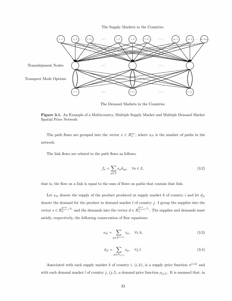
����1, 1 ����1, 2 · · ·����1, k1
The Supply Markets in the Countries
· · · ����i, 1 ����i, 2 · · ·����i, ki · · · ����m, 1 ����m, 2 · · ·����m, km
Transshipment Nodes
Transport Mode Options
���� ����· · · · · · ����
����1, 1 ����· · · j, lj · · · ����n, ln
The Demand Markets in the Countries
SSSSSSw?
������/
SSSSSSw?
������/
SSSSSSw?
������/
Figure 3.1. An Example of a Multicountry, Multiple Supply Market and Multiple Demand MarketSpatial Price Network
The path flows are grouped into the vector x ∈ RnP+ , where nP is the number of paths in the
network.
The link flows are related to the path flows as follows:
fa =∑p∈P
xpδap, ∀a ∈ L, (3.2)
that is, the flow on a link is equal to the sum of flows on paths that contain that link.
Let sik denote the supply of the product produced at supply market k of country i and let djl
denote the demand for the product in demand market l of country j. I group the supplies into the
vector s ∈ R∑m
i=1 ki+ and the demands into the vector d ∈ R
∑nj=1 lj
+ . The supplies and demands must
satisfy, respectively, the following conservation of flow equations:
sik =∑
p∈P (i,k)
xp, ∀i, k, (3.3)
djl =∑
p∈P(j,l)
xp, ∀j, l. (3.4)
Associated with each supply market k of country i, (i, k), is a supply price function π(i,k) and
with each demand market l of country j, (j, l), a demand price function ρ(j,l). It is assumed that, in
33
general, the supply price at a supply market in a country can depend on the vector of supplies and
that the demand price at a demand market in a country can depend on the vector of demands so
that:
π(i,k) = π(i,k)(s), ∀i, k, (3.5)
ρ(j,l) = ρ(j,l)(d), ∀j, l. (3.6)
These functions are assumed to be continuous with the supply price functions being monotonically
increasing and the demand functions, on the other hand, monotonically decreasing.
Furthermore, a unit cost ca associated with each link a in the network, which includes the unit
transportation cost, and, in general, can depend on the vector of link flows f , so that:
ca = ca(f), ∀a ∈ L. (3.7)
The link cost functions are also assumed to be continuous and monotonically increasing in order
to capture congestion.
The unit cost on a path p, Cp, joining a supply market in a country with a demand market in a
country is then given by:
Cp =∑a∈L
ca(f)δap, ∀p ∈ P. (3.8)
Hence, the cost on a path is equal to the sum of the costs on the links that make up the path.
I now introduce the additional notation for the tariff-rate quotas. Recall that a tariff quota is a
two-tiered tariff. Let τuGgdenote the tariff, which is fixed and preassigned to group Gg, when the sum
of the path flows of the product in the group is less than (under) the quota QGg, for g. Also, let τoGg
denote the fixed and preassigned tariff, which is assigned to group Gg if the sum of the path flows
of the product in the group is greater than QGg , for all g, and τoGg> τuGg
. In addition, it is worth
mentioning that the under tariffs can be set to zero, depending on the application. Let λGg, for all
Gg, denote the quota rent equivalent (see, e.g., Skully (2001)), which can have an interpretation of
a Lagrange multiplier. Additionally, the quota rent equivalents are grouped into the vector λ ∈ Rh.
The costs, prices, and tariffs are all in a common currency.
34
• Definition 3.1: Spatial Price Network Equilibrium Conditions Under Tariff Rate
Quotas
A product flow pattern x∗ ∈ RnP+ and quota rent equivalent λ∗ ∈ Rh is a spatial price network
equilibrium under a tariff-rate quota regime if the following conditions hold: For all groups Gg,
for all g, and for all pairs of supply and demand markets in the countries: (i, j), (k, l) ∈ Gg,
and all paths p ∈ P (i,k)(j,l) :
π(i,k) + Cp + τuGg+ λ∗Gg
= ρ(j,l), if x∗p > 0,
≥ ρ(j,l), if x∗p = 0,
(3.9)
and for all g:
λ∗Gg
= τoGg
− τuGg, if
∑p∈PGg
x∗p > QGg,
≤ τoGg− τuGg
, if∑p∈PGg
x∗p = QGg,
= 0, if∑p∈PGg
x∗p < QGg .
(3.10)
Equilibrium conditions (3.9) are an expansion of the Samuelson (1952) and Takayama and Judge
(1971) spatial price equilibrium conditions to include, in a novel manner, the incorporation of two-
tiered tariffs, depending on the volumes of product flows and quotas in country groups, as stated in
(3.10). See also path formulations of classical spatial price equilibrium problems using path flows
by Florian and Los (1982) and Dafermos and Nagurney (1983). Note that, according to the above
definition, if the sum of the product path flows is less than the imposed quota for the particular
group of countries, then the assigned tariff on those paths is just equal to the “under” quota tariff
τuGgsince in this case λ∗Gg
= 0. On the other hand, if the sum of the path flows exceeds the quota
(which is allowed in the case of tariff quotas), then the incurred tariff on the associated paths is
equal to the “over” quota tariff τoGg. If the sum of the path flows is precisely equal to the quota for
the group then the incurred additional payment on the corresponding paths is less than τuGg.
• Remark 3.1
In the case of a domestic group Gg, the above conditions (3.9) and (3.10) are also applicable (and
this feature is illustrated in simple numerical examples in Section 3.2.1), where I set τuGg= 0, and
τoGg> τuGg
, with QGgvery large, so that it is never achievable.
35
In view of (3.3) and (3.5), the supply price functions can be redefined as:
π(i,k)(x) ≡ π(i,k)(s), ∀i, k, (3.11)
the demand price functions, in view of (3.4) and (3.6), as:
ρ(j,l)(x) ≡ ρ(j,l)(d), ∀j, l, (3.12)
and, in view of (3.2), (3.7), and (3.8), the path and link cost functions:
Cp(x) ≡∑a∈L
ca(x)δap, ∀p ∈ P, (3.13)
where
ca(x) ≡ ca(f), ∀a ∈ L. (3.14)
The above definitions allow us to construct a variational inequality formulation of the governing
spatial price network equilibrium conditions under a tariff-rate quota regime in path flows and quota
rents in the Theorem below. The feasible set is defined as K ≡ {(x, λ)|x ∈ RnP+ , λ ∈ Rh+|0 ≤ λGg ≤
τoGg− τuGg
,∀g}.
• Theorem 3.1: Variational Inequality Formulation of Spatial Price Network Equi-
librium Conditions Under Tariff Rate Quotas
A path flow and quota rent equivalent pattern (x∗, λ∗) ∈ K is a spatial price network equilibrium
under a tariff quota regime according to Definition 3.1 if and only if it satisfies the variational
inequality:
∑g
∑(i,j)∈Gg
∑k∈Oi
∑l∈Dj
∑p∈P (i,k)
(j,l)
[π(i,k)(x∗) + Cp(x
∗) + τuGg+ λ∗Gg
− ρ(j,l)(x∗)]×[xp − x∗p
]
+∑g
QGg−∑p∈PGg
x∗p
× [λGg− λ∗Gg
]≥ 0, ∀(x, λ) ∈ K. (3.15)
Proof: First necessity conditions are established, that is, I prove that if a path flow and quota
rent equivalent pattern (x∗, λ∗) ∈ K satisfies Definition 3.1 then it also satisfies the variational
inequality (3.15). Note that equilibrium conditions (3.9), in view of (3.11) – (3.14), can be
36
rewritten as: For all groups Gg, for all g, and for all pairs of supply and demand markets:
(i, j), (k, l) ∈ Gg, and all paths p ∈ P (i,k)(j,l) :
π(i,k)(x∗) + Cp(x∗) + τuGg
+ λ∗Gg
= ρ(j,l)(x
∗), if x∗p > 0,
≥ ρ(j,l)(x∗), if x∗p = 0.
(3.16)
Clearly, for a fixed path p ∈ P (i,k)(j,l) with (i, k), (j, l) ∈ Gg, and group Gg, (3.16) implies that
[π(i,k)(x∗) + Cp(x
∗) + τuGg+ λ∗Gg
− ρ(j,l)(x∗)]×[xp − x∗p
]≥ 0, ∀xp ≥ 0, (3.17)
since, according to Definition 3.1, if x∗p > 0, then [π(i,k)(x∗) + Cp(x∗) + τuGg
+Gg∗ −ρ(j,l)(x∗)] = 0,
and (3.17) holds; on the other hand, if x∗p = 0, then [π(i,k)(x∗) + Cp(x∗)+ τuGg
+ λ∗Gg− ρ(j,l)(x∗)]≥0,
and since, due to the nonnegativity assumption on the path flows:[xp − x∗p
]≥ 0; hence, the product
of these two terms is also ≥ 0, so (3.17) also holds in this case. Inequality (3.17) is independent of
path p and, therefore, I can sum (3.17) over all paths, obtaining:
∑g
∑(i,j)∈Gg
∑k∈Oi
∑l∈Dj
∑p∈P (i,k)
(j,l)
[π(i,k)(x∗) + Cp(x
∗) + τuGg+ λ∗Gg
− ρ(j,l)(x∗)]×[xp − x∗p
]≥ 0,
∀x ∈ K. (3.18)
Also, for a fixed g, (3.10) in Definition 3. 1 implies that:
QGg−∑p∈PGg
x∗p
× [λGg− λ∗Gg
]≥ 0, 0 ≤ λGg
≤ τoGg− τuGg
. (3.19)
Indeed, according to (3.10), if λ∗Gg= τoGg
− τuGg, then the expression before the multiplication
sign in (3.19) is negative, whereas that after the multiplication sign is less than equal to zero and,
thus, (3.19) holds. If λ∗Gg= 0, then according to (3.10) the first term in (3.19) is nonnegative
and, due to feasibility, so is the second term; therefore, their product is nonnegative and (3.19) also
holds. Finally, if∑p∈PGg
x∗p = Qg, then, according to (3.10), the term to the right-hand-side of the
multiplication sign in (3.19) can be positive or negative, but the multiplication of both terms is still
equal to zero and (3.19) holds.
37
The inequality (3.19) holds for any g, and, therefore, I can conclude that summation over all g
yields: ∑g
QGg−∑p∈PGg
x∗p
× [λGg− λ∗Gg
]≥ 0, ∀λ ∈ K. (3.20)
Summation of (3.18) and (3.20) gives us variational inequality (3.15) and necessity is established.
I now prove sufficiency, that is, a solution (x∗, λ∗) ∈ K of variational inequality (3.15) also
satisfies the supply chain network equilibrium conditions (3.9) and (3.10) of Definition 3.1.
Assume that a pattern (x∗, λ∗) ∈ K satisfies variational inequality (3.15). Let λGg= λ∗Gg
for all
g and let xq = x∗q for all paths q except for path p ∈ P (i,k)(j,l) . Substitution of these into (3.15) then
yields: [π(i,k)(x∗) + Cp(x
∗) + τuGg+ λ∗Gg
− ρ(j,l)(x∗)]×[xp − x∗p
]≥ 0, ∀xp ≥ 0. (3.21)
But (3.21) implies that equilibrium conditions (3.9) must hold for path p and, hence, for any
path.
Similarly, setting xp = x∗p, ∀p ∈ P , and λGg = λ∗Ggfor all g 6= r, and substituting the resultants
into variational inequality (3.15) gives us:
QGr −∑p∈PGr
x∗p
× [λGr − λ∗Gr
]≥ 0, ∀λGr such that 0 ≤ λGr ≤ τoGr
− τuGr. (3.22)
And (3.22) implies that equilibrium conditions (3.10) must hold for any r. The proof is complete.
2
I now put variational inequality (3.15) into standard form as shown in Chapter 2 equation 2.1a:
determine X∗ ∈ K ⊂ RN , such that
〈F (X∗), X −X∗〉 ≥ 0, ∀X ∈ K. (3.23)
where X and F (X) are N -dimensional vectors, K is a closed, convex set, and F is a given continuous
function from K to RN . Indeed, I can define X ≡ (x, λ) and F (X) ≡ (F1(X), F2(X)), where F1(X)
consists of nP elements: π(i,k)(x) + Cp(x) + τuGg+ λGg
− ρ(j,l)(x), for all paths p ∈ P , and F2(X)
consists of h elements, with the g-th element given by: QGg −∑p∈PGg
xp. Also, here N = nP + h
and K ≡ K.
38
3.2. Variants of the Spatial Price Network Equilibrium Model
In this section, I present several variants of the model constructed in Section 3.1. This is being
done in order to demonstrate the flexibility of the variational inequality formalism for policy modeling
in the context of world trade.
First, an extension of the classical spatial price network equilibrium model is given, and from
this model policies in the form of ad valorem tariffs and then quotas incorporated.
Without loss of generality, let the set of paths P correspond to all the paths joining the country
supply market nodes with the country demand market nodes with the number of paths being nP .
In the absence of a tariff-rate quota regime, the following definition is obtained, with reference to
(3.16):
• Definition 3.2: (Classical) Spatial Price Network Equilibrium Conditions
A product flow pattern x∗ ∈ RnP+ is a spatial price network equilibrium if the following condi-
tions hold: For all pairs of supply and demand markets (i, k), (j, l) and all paths p ∈ P (i,k)(j,l) :
π(i,k)(x∗) + Cp(x∗)
= ρ(j,l)(x
∗), if x∗p > 0,
≥ ρ(j,l)(x∗), if x∗p = 0.
(3.24)
The following variational inequality is immediate using similar arguments as in the proof of
Theorem 3.1.
• Corollary 3.1: Variational Inequality Formulation of a Spatial Price Network Equi-
librium
A product flow pattern x∗ ∈ RnP+ is a spatial price network equilibrium according to Definition
3.2 if and only if it satisfies the variational inequality:
∑(i,k)
∑(j,l)
∑p∈P (i,k)
(j,l)
[π(i,k)(x∗) + Cp(x
∗)− ρ(j,l)(x∗)]×[xp − x∗p
]≥ 0, ∀x∗ ∈ RnP
+ . (3.25)
• Remark 3.2
There are alternative variational inequalities to (3.25). The first alternative would utilize the
conservation of flow equations and vectors s and d and retain the path flows; the second alternative
39
formulation would then further utilize the link/path conservation of flow equations and have the
supplies, demands, and link flows be the variables. For an example of a model with the latter, but
not including explicit countries and regions, see Nagurney (1999).
Also, unit tariffs can be easily incorporated into the variational inequality (3.25) by simply adding
the tariff on the appropriate link(s) of the appropriate paths.
Ad valorem tariffs are now considered, with 1 + τij ; i = 1, . . . ,m; j = 1, . . . , n, denoting the ad
valorem tariff associated with product flows from country i to j as in the modification of Definition
3.2 to yield Definition 3.3 below. Typically, the τijs are in the range 0 < τij ≤ 1.
• Definition 3.3: Spatial Price Network Equilibrium Conditions with Ad Valorem
Tariffs
A product flow pattern x∗ ∈ RnP+ is a spatial price network equilibrium under an ad valorem
tariff regime if the following conditions hold: For all pairs of supply and demand markets
(i, k), (j, l) and all paths p ∈ P (i,k)(j,l) :
(π(i,k)(x∗) + Cp(x∗))(1 + τij)
= ρ(j,l)(x
∗), if x∗p > 0,
≥ ρ(j,l)(x∗), if x∗p = 0.
(3.26)
The following corollary generalizes results of Nagurney, Nicholson, and Bishop (1996a,b) to
multiple countries and multiple paths connecting each pair of supply and demand markets as well
as non-fixed transportation costs.
• Corollary 3.2: Variational Inequality Formulation of a Spatial Price Network Equi-
librium with Ad Valorem Tariffs
A product flow pattern x∗ ∈ RnP+ is a spatial price network equilibrium under an ad valorem
tariff regime according to Definition 3.3 if and only if it satisfies the variational inequality:
∑(i,k)
∑(j,l)
∑p∈P (i,k)
(j,l)
[(π(i,k)(x∗) + Cp(x
∗))(1 + τij)− ρ(j,l)(x∗)]×[xp − x∗p
]≥ 0, ∀x∗ ∈ RnP
+ .
(3.27)
40
I now consider strict quotas. Note that, in contrast, under a tariff-rate quota regime, the tariffs
are two-tiered, and the quota can be exceeded, but then there is a higher associated tariff. In
practice, these can be set very high.
Specifically, let ˆQg denote the strict quota for g; g = 1, . . . , h and let λGgdenote the tariff/tax,
which is, in effect, a Lagrange multiplier, and I refer to it as such, if the quota is reached for group
Gg. Then I have the following spatial price network equilibrium conditions:
• Definition 3.4: Spatial Price Network Equilibrium Conditions Under Strict Quotas
A product flow pattern x∗ ∈ RnP+ and Lagrange multiplier pattern λ∗ ∈ Rh+ is a spatial price
network equilibrium under strict quotas if the following conditions hold: For all pairs of supply
and demand markets (i, k), (j, l) and all paths p ∈ P (i,k)(j,l) :
π(i,k)(x∗) + Cp(x∗) + λ∗
Gg
= ρ(j,l)(x
∗), if x∗p > 0,
≥ ρ(j,l)(x∗), if x∗p = 0,
(3.28)
and for all g:
λ∗Gg
≥ 0, if
∑p∈PGg
x∗p = ˆQGg,
= 0, if∑p∈PGg
x∗p <ˆQGg
.
(3.29)
The following corollary follows using similar arguments as in the proof of Theorem 3.1.
• Corollary 3.3: Variational Inequality Formulation of a Spatial Price Network Equi-
librium with Strict Quotas
A product flow pattern x∗ ∈ RnP+ and Lagrange multiplier pattern λ∗ ∈ Rh+ is a spatial price
network equilibrium under strict quotas according to Definition 3.4 if and only if it satisfies
the variational inequality:
∑(i,k)
∑(j,l)
∑p∈P (i,k)
(j,l)
[π(i,k)(x∗) + Cp(x
∗) + λ∗Gg− ρ(j,l)(x∗)
]×[xp − x∗p
]
+∑g
ˆQGg−∑p∈PGg
x∗p
× [λGg − λ∗Gg
]≥ 0, ∀x∗ ∈ RnP
+ ,∀λ∗ ∈ Rh+. (3.30)
41
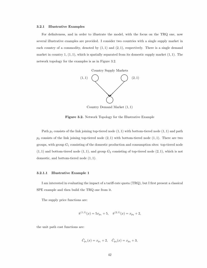
3.2.1 Illustrative Examples
For definiteness, and in order to illustrate the model, with the focus on the TRQ one, now
several illustrative examples are provided. I consider two countries with a single supply market in
each country of a commodity, denoted by (1, 1) and (2, 1), respectively. There is a single demand
market in country 1, (1, 1), which is spatially separated from its domestic supply market (1, 1). The
network topology for the examples is as in Figure 3.2.
����Country Demand Market (1, 1)
@@@@@
���
��R
(1, 1) ���� ����(2, 1)
Country Supply Markets
Figure 3.2. Network Topology for the Illustrative Example
Path p1 consists of the link joining top-tiered node (1, 1) with bottom-tiered node (1, 1) and path
p2 consists of the link joining top-tiered node (2, 1) with bottom-tiered node (1, 1). There are two
groups, with group G1 consisting of the domestic production and consumption sites: top-tiered node
(1, 1) and bottom-tiered node (1, 1), and group G2 consisting of top-tiered node (2, 1), which is not
domestic, and bottom-tiered node (1, 1).
3.2.1.1 Illustrative Example 1
I am interested in evaluating the impact of a tariff-rate quota (TRQ), but I first present a classical
SPE example and then build the TRQ one from it.
The supply price functions are:
π(1,1)(x) = 5xp1 + 5, π(2,1)(x) = xp2 + 2,
the unit path cost functions are:
Cp1(x) = xp1 + 2, Cp2(x) = xp2 + 3,
42
and the demand price function is:
ρ(1,1)(x) = −(xp1 + xp2) + 18.
Observe that the non-domestic supply market has a lower supply market price function but a
higher unit transportation cost function than the domestic supply and demand markets.
In the classical model, without any imposed TRQs, the spatial price equilibrium conditions,
according to (3.24), are, with the realization that x∗p1 > 0 and x∗p2 > 0:
π(1,1)(x∗) + Cp1(x∗) = ρ(1,1)(x∗),
π(2,1)(x∗) + Cp2(x∗) = ρ(1,1)(x∗),
and, hence, the following is obtained, at equilibrium:
5x∗p1 + 5 + x∗p1 + 2 = −(x∗p1 + x∗p2) + 18,
x∗p2 + 2 + x∗p2 + 3 = −(x∗p1 + x∗p2) + 18,
which, after algebraic simplification, results in the following system of equations:
7x∗p1 + x∗p2 = 11,
x∗p1 + 3x∗p2 = 13,
with solution: x∗p1 = 1 and x∗p2 = 4, with π(1,1) = 10, Cp1 = 3, and ρ(1,1) = 13, and π(2,1) = 6,
Cp2 = 7, so, indeed, the classical spatial price equilibrium conditions are satisfied (cf. (3.24)).
The following tariff-rate quota is now imposed, which allows, once the problem is solved, to
investigate the impacts on trade flows and incurred prices.
For the domestic pair, there is no under tariff, and the over tariff, which will never be applied,
since I impose a very high quota, is as follows:
τuG1= 0, τoG1
= 1, QG1= 100,
43
and for the non-domestic, domestic pair of nodes, the tariffs and associated quota are:
τuG2= 2, τoG2
= 4, QG2= 3.
Returning to the governing equilibrium conditions for the SPE model with TRQs, given by (3.9)
and (3.10), and knowing that λ∗G1= 0, now, the following equations must be satisfied:
5x∗p1 + 5 + x∗p1 + 2 = −(x∗p1 + x∗p2) + 18,
x∗p2 + 2 + x∗p2 + 3 + τuG2+ λ∗G2
= −(x∗p1 + x∗p2) + 18.
Moreover, if x∗p2 = 3, then λ∗G2= τoG2
− τuG2≤ 2. Substituting x∗p2 = 3 into the above system of
equations, the following is obtained:
7x∗p1 + 3 = 11,
x∗p1 + 9 + λ∗G2= 11.
Solving now the above simplified system:
x∗p1 = 11
7, λ∗G2
=6
7,
since x∗p2 = 3.
Observe that, by imposing the TRQ, as above, the domestic supply market now produces more
than in the classical SPE numerical example above, whereas the non-domestic supply market exports
less. The consumers, nevertheless, now pay a higher unit price of ρ(1,1) = 13 67 as opposed to 13.
Also, now have: π(1,1) = 10 57 , Cp1 = 3 1
7 , and π(2,1) = 5, Cp2 = 6.
3.2.1.2 Illustrative Example 2
I construct another TRQ example and the network topology is as in Figure 3.2. The same
markets are domestic as in Illustrative Example 3.1.
44
The supply price functions are now:
π(1,1)(x) = 3xp1 + 1, π(2,1)(x) = xp2 + 1,
the unit path cost functions are:
Cp1(x) = 2xp1 + 1, Cp2(x) = xp2 + 1,
and the demand price function is:
ρ(1,1)(x) = −2(xp1 + xp2) + 26.
Proceeding as in Example 3.1, and realizing that x∗p1 > 0 and x∗p2 > 0, the classical SPE
conditions (3.24) yield a system of equations, which, when solved algebraically, yield the following
solution: x∗p1 = 2 and x∗p2 = 5, with the following incurred supply prices, unit path transportation
costs, and demand price: π(1,1) = 7, Cp1 = 5, and ρ(1,1) = 12, and π(2,1) = 6, Cp2 = 6. Clearly, the
classical spatial price equilibrium conditions are satisfied (cf. (3.24)).
Now the following tariff-rate quota is imposed, with: τuG2= 3, τoG2
= 6, and QG2= 2.
Utilizing TRQ equilibrium conditions (3.9) and (3.10), the solution is: x∗p1 = 2 12 , x∗p2 = 3 1
4 > 2,
and λ∗G2= 3. Observe that, in this example, the imports from the second supply market, which is
not domestic, exceeds the imposed quota and, therefore, the higher tariff is in effect. The incurred
prices and costs are: π(1,1) = 8 12 , Cp1 = 6, and ρ(1,1) = 14 1
2 , and π(2,1) = 4 14 , Cp2 = 4 1
4 . The
supply price at the domestic supply market has increased, whereas that of the non-domestic one has
decreased. More of the domestic product is consumed than previously without the TRQ and less of
the non-domestic one. Again, the consumers experience a higher demand market price.
3.3. Qualitative Properties
In this section, I provide qualitative properties of the function F (cf. (3.23)) corresponding to
the SPE model with TRQs, which are needed for convergence of the algorithmic scheme in Section
3.4. In addition, existence results for a solution X∗ of the variational inequality (3.23) are provided.
In the following proposition I establish that if the supply price functions, the link cost functions,
and minus the demand price functions are monotone in their respective vectors of variables, then
45
the function F as in (3.23) is monotone in (X,λ). Conditions that guarantee monotonicity of these
functions is that their respective Jacobian matrices are positive semidefinite over the feasible set.
In the proof of Proposition 3.1 I also derive an alternative variational inequality to (3.15), which
includes link flows. Hence, the feasible set i defined as K1 ≡ {(s, f, d, x, λ)|x ∈ RnP+ , λ ∈ Rh+, 0 ≤
λGg ≤ τoGg− τuGg
,∀g, and (3.2), (3.3), (3.4) hold}.
• Proposition 3.1: Monotonicity of F (X) in (3.23)
Assume that the vector of supply price functions, π(s), the vector of link transportation cost
functions, c(f), and the vector of minus the demand price functions −ρ(d), are all monotone
(cf. Definition 2.3) as follows:
〈π(s1)− π(s2), s1 − s2〉 ≥ 0, ∀(s1, s2) ∈ K1, (3.31a)
〈c(f1)− c(f2), f1 − f2〉 ≥ 0, ∀(f1, f2) ∈ K1, (3.31b)
−〈ρ(d1)− ρ(d2), d1 − d2〉 ≥ 0, ∀(d1, d2) ∈ K1. (3.31c)
Then the function that enters the VI (3.15), as in standard form F (X) in (3.23), is monotone,
with respect to the path flows x and the Lagrange multipliers λ, X = (x, λ).
Proof: Using (3.2), (3.3), (3.4), (3.7), and (3.8), and recalling that Gg ∩Gh = ∅,∀g 6= h, ∀g, h, and
the following equations:
sik =∑
p∈P(i,k)
xp =
n∑j=1
lj∑l=1
∑p∈P (i,k)
(j,l)
xp =∑g
∑(i,j)∈Gg
∑l∈Dj
∑p∈P (i,k)
(j,l)
xp, (3.32)
djl =∑
p∈P(j,l)
xp =
m∑i=1
ki∑k=1
∑p∈P (i,k)
(j,l)
xp =∑g
∑(i,j)∈Gg
∑k∈Oi
∑p∈P (i,k)
(j,l)
xp, (3.33)
and ∑g
∑(i,j)∈Gg
∑k∈Oi
∑l∈Dj
∑p∈P (i,k)
(j,l)
Cp(x∗)×
[xp − x∗p
]=∑p∈P
Cp(x)×[xp − x∗p
]
=∑p∈P
[∑a∈L
ca(f)δap
]×[xp − x∗p
]=∑a∈L
ca(f)×
∑p∈P
δapxp −∑p∈P
δapx∗p
=∑a∈L
ca(f)× [fa − f∗a ] .
(3.34)
46
Using now (3.32), (3.33), and (3.34), and also (3.11) and (3.12), VI (3.15) is rewritten as follows:
∑g
∑(i,j)∈Gg
∑k∈Oi
∑l∈Dj
∑p∈P (i,k)
(j,l)
π(i,k)(x∗)×[xp − x∗p
]
+∑g
∑(i,j)∈Gg
∑k∈Oi
∑l∈Dj
∑p∈P (i,k)
(j,l)
Cp(x∗)×
[xp − x∗p
]+∑g
∑(i,j)∈Gg
∑k∈Oi
∑l∈Dj
∑p∈P (i,k)
(j,l)
[τuGg
+ λ∗Gg
]×[xp − x∗p
]−∑g
∑(i,j)∈Gg
∑k∈Oi
∑l∈Dj
∑p∈P (i,k)
(j,l)
ρ(j,l)(x∗)×
[xp − x∗p
]
+∑g
QGg−∑p∈PGg
x∗p
× [λGg− λ∗Gg
]=∑i,k
π(i,k)(s∗)× [sik − s∗ik] +∑a∈L
ca(f∗)× [fa − f∗a ]
+∑g
∑p∈Gg
[τuGg
+ λ∗Gg
]×[xp − x∗p
]−∑j,l
ρ(j,l)(d∗)×
[djl − d∗jl
]
+∑g
QGg−∑p∈PGg
x∗p
× [λGg− λ∗Gg
]≥ 0, ∀(s, f, d, x, λ) ∈ K1. (3.35)
Now I can prove that F (X) is monotone. For any X1 = (x1, λ1), X2 = (x2, λ2) ∈ K,
〈F (X)1 − F (X2), X1 −X2〉 = 〈(F (x1, λ1)− F (x2, λ2)),
x1 − x2
λ1 − λ2
〉
=∑i,k
([π(i,k)(s1)− π(i,k)(s2)
]×[s1ik − s2ik
]+∑a∈L
[ca(f1)− ca(f2)
]×[f1a − f2a
]
+∑g
[λ1Gg− λ2Gg
]×
∑p∈PGg
x1p −∑p∈PGg
x2p
−∑j,l
[ρ(j,l)(d
1)− ρ(j,l)(d2)]×[d1jl − d2jl
]
+∑g
− ∑p∈PGg
x1p +∑p∈PGg
x2p
× [λ1Gg− λ2Gg
]=∑i,k
[π(i,k)(s1)− π(i,k)(s2)
]×[s1ik − s2ik
]+∑a∈L
[ca(f1)− ca(f2)
]×[f1a − f2a
]−∑j,l
[ρ(j,l)(d
1)− ρ(j,l)(d2)]×[d1jl − d2jl
]. (3.36)
With the assumptions (3.31a, b, c) on the functions in the statement of Proposition 3.1, I can
conclude that expression (3.36) is greater or equal to zero. Thus, F (X) is monotone. 2
47
In addition, I can expect that F (X) for the model is Lipschitz continuous under assumptions
that the underlying supply price, demand price, and link cost functions are continuous and have
bounded second order derivatives (cf. Definition 2.6). The definition of Lipschitz continuity is given
below for easy reference.
• Definition 3.5: Lipschitz Continuity
A function F (X) is Lipschitz continuous if the following condition holds:
‖F (X ′)− F (X ′′)‖ ≤ L‖X ′ −X ′′‖, ∀X ′, X ′′ ∈ K, (3.37)
where L > 0 is known as the Lipschitz constant.
For convergence of the algorithmic scheme described in the next Section, which I utilize for
computational purposes in the case study, only monotonicity and Lipschitz continuity of F (X) are
required, provided that a solution exists.
I now turn to establishing the existence of a solution X∗ to VI (3.15); equivalently, (3.23). Note
that the feasible set K is not compact and, hence, existence of a solution would not immediately
follow from the classical theory of variational inequalities (see Kinderlehrer and Stampacchia (1980))
although the supply price, demand price, and link cost functions are assumed to be continuous.
• Theorem 3.5: Existence of a Solution
Existence of a solution X∗ to the VI for the model given by (3.15); equivalently, (3.23), is
guaranteed.
Proof: I know that the quota rent equivalents comprising the vector λ are bounded because of
the definition of the feasible set K. The demands, in turn, are bounded since the demand prices
are monotonically decreasing and negative prices are not relevant. Furthermore, although demands
may be large they will not be infinite since the population and, hence, demand, is bounded at each
demand market. Therefore, the product path flows are also bounded and, consequently, existence
of a solution X∗ is guaranteed.
3.4. The Algorithm
In this section, the realization of the modified projected method (cf. Section 2.4.2) for the
computation of the variational inequality (3.23), equivalently (3.15), governing the spatial equilib-
48
rium model with tariff-rate quotas and its variants, is described. Below, I present each step of the
computation with respect to this model and provide the explicit formulae.
Step 0: Initialization
Set (x0, λ0) ∈ K. Let t = 1 and set ϕ so that 0 < ϕ ≤ 1L .
Step 1: Construction and Computation
Compute (xt, λt) ∈ K by solving the variational inequality subproblem:
∑g
∑(i,j)∈Gg
∑k∈Oi
∑l∈Dj
∑p∈P (i,k)
(j,l)
[ xtp+ϕ(π(i,k)(xt−1)+Cp(xt−1)+τuGg
+λt−1Gg−ρ(j,l)(xt−1))−xt−1p ]×[ xp−xtp]
+∑g
λtGg+ ϕ(QGg
−∑p∈PGg
xt−1p )− λt−1Gg
× [λGg− λtGg
]≥ 0, ∀(x, λ) ∈ K. (3.38)
Step 2: Adaptation
Compute (xt, λt) ∈ K by solving the variational inequality subproblem:
∑g
∑(i,j)∈Gg
∑k∈Oi
∑l∈Dj
∑p∈P (i,k)
(j,l)
[ xtp +ϕ(π(i,k)(xt) + Cp(xt) + τuGg
+ λtGg− ρ(j,l)(xt))−xt−1p ] × [ xp−xtp]
+∑g
λtGg+ ϕ(QGg
−∑p∈PGg
xtp)− λt−1Gg
× [λGg− λtGg
]≥ 0, ∀(x, λ) ∈ K. (3.39)
Step 3: Convergence Verification
If |xtp − xpt−1| ≤ ε, for all p ∈ P (i,k)(j,l) , ∀i, k, j, l, and |λtGg
− λGg
t−1| ≤ ε, for all g = 1, . . . , h, with
ε > 0, a specified tolerance, then, stop; otherwise, set t := t+ 1 and go to Step 1.
3.4.1 Closed Form Expressions
I present the closed form expressions for the solution of problems (3.38). Analogous ones for
(3.39) can be determined accordingly.
The closed form expressions for the path flows at iteration t are as follows.
49
For each path p ∈ P (i,k)(j,l) , ∀i, k, j, l, compute:
xtp = max{0, ϕ(ρ(j,l)(xt−1p )− π(i,k)(xt−1)− Cp(xt−1)− τuGg
− λt−1Gg) + xt−1p }, (3.40)
and the following is the closed form expression for all the quota rent equivalents for group Gg;
g = 1, . . . , h:
λtGg= max{0,min{ϕ(
∑p∈PGg
xt−1p − QGg+ λt−1Gg
), τoGg− τuGg
}}. (3.41)
I now provide the convergence result for the modified projection method.
• Theorem 3.6: Convergence
Assume that the function F (X) that enters the variational inequality (3.23) (or (3.15)) satisfies
the conditions in Proposition 3.1 and following, that is, monotonicity and Lipschitz continuity.
Then, the modified projection method described above converges to a solution of the variational
inequality (3.23), or equivalently (3.15).
Proof: As stated in Korpelevich (1977), the modified projection method converges to the solution
of the variational inequality problem (3.23) (or (3.15)), provided that the function F that enters the
variational inequality is monotone and Lipschitz continuous and that a solution exists. 2
3.5. A Case Study on the Dairy Industry
In this section, I focus on a case study based on the dairy industry in the United States. In 2002,
the dairy industry in the United States generated 20 billion dollars in sales value (Hadjigeorgalis
(2005)). In recent years, the dairy industry in the United States has experienced a shift towards
larger operations with more than 500 cows, in which the dairy farmers can hold more inventory and
increase their production of milk. The large size operations accounted for nearly 60% of all milk
produced in 2009, a substantial increase from 39% in 2001 (USDA (2018)). The dairy production
in the US occurs primarily in the states of: California, Wisconsin, New York, Pennsylvania, Idaho,
Minnesota, New Mexico, Michigan, Texas, and Washington (NASS (2004), USDA (2018)). Since
2002, the US is a net importer of dairy products, especially of cheese, according to Hadjigeorgalis
(2005). The international trade in the dairy industry is governed by the 1994 Uruguay Round of
Multilateral Trade Negotiations (cf. United States. Office of the U.S. Trade Representative (1994)).
Furthermore, in the United States tariff-rate quotas are imposed on most of the dairy products. The
50
US is an exporter of some dairy products such as dry nonfat milk products, with the major export
market for the United States of nonfat dry milk being Mexico.
For the case study, I focus on the dairy industry, specifically, on cheese in the United States.
Cheese is usually contained in a preserved form in which the main protein and milk fat are not
exposed to rapid deterioration from microorganisms. According to Hadjigeorgalis (2005), the Euro-
pean Union dominates the cheese market in the United States by having an import value of 69%,
where the closest export country is New Zealand with only 10%. Therefore, it is clear that the
European Union and the United States engage in a crucial amount of agricultural trade and it is
worthwhile to analyze this relationship in this case study. Especially, in 2018, with the ongoing
trade wars (see Tankersley (2018)) and disputes between many countries all over the world, I believe
that a case study on the dairy industry and the evaluation of the impact of tariff-rate quotas are
worth investigating (cf. Paquette, Lynch, and Rauhala (2018)). Furthermore, according to Chatel-
lier (2016), the Netherlands, Germany, and France are the top exporters of dairy products in the
European Union, and cheese is counted as the top dairy product exported from France. Therefore,
for this case study, I focus on France as a producing country from the European Union.
I implemented the modified projection method in MATLAB on an OS X 10.12.6 system. The
code in Matlab is executed on a Macbook Pro laptop with a 2.8 GHz Intel Core i5 processor and
8GB 1600 MHz DDR3 memory. The parameter ϕ is set to 0.3 with the convergence tolerance being
10−6, that is, the modified projection method is deemed to have converged if the absolute value of
the difference of each successive variable iterate differs by no more than this value. The algorithm
was initialized with each path flow set equal to 1, and with each quota rent equivalent (the Lagrange
multiplier) for the variational inequality (3.15) set equal to 0. In the following examples I modify
the spatial price network and also the associated tariff values to generate insights.
3.5.1 Baseline Example
The first example serves as a baseline example. The computations are made utilizing the closed
form expressions provided for the modified projection method in Section 3.4. The spatial price
network structure for the Baseline Example is given in Figure 3.3. For this example, the producing
countries are the United States and France, which belongs to the European Union, with each having
two supply markets. Furthermore, The United States has supply markets: Southwest and Midwest,
represented in Figure 3 by the top-tiered nodes (1, 1) and (1, 2), respectively, whereas France has
51

supply markets: South and North, represented, respectively, by the top-tiered nodes (2, 1) and (2, 2)
in Figure 3.3.
The transshipment node is assumed to be located in the East region of the United States, with
the cheese from the South and the North regions of France arriving in the East region of the United
States, and then being transported to the demand markets. Furthermore, I assume that cheese
produced at a dairy farm in the Southwest and the Midwest of the United States is sent to the
East region of the United States to be distributed to the demand markets. The United States has
three demand markets, depicted by the bottom-tiered nodes in Figure 3.3: (1, 2), (1, 3), and (1, 4),
corresponding, without loss of generality to: the Midwest, the Northeast, and the Southeast of the
United States, respectively.
There are two groups, G1 and G2. The first group, G1, contains the domestic supply markets
and demand markets in the United States, and includes the nodes (1, 1), (1, 2) (both supply and
demand ones), (1, 3), and (1, 4). The group G2 represents the supply markets in France, specifically,
the South and the North, and the demand markets in the US, represented by the bottom-tiered
nodes in Figure 3.3: (1, 2), (1, 3), and (1, 4). The examples are constructed from the data collected
from the website of the European Commission (2018). I also retrieved information from the United
Nations (M49) area tool (cf. United Nations (1999)), in which they define countries and regions for
regional and preferential trade agreements.
����1, 1 ����1, 2
1 2 3 4
56 7
8
United States
Southwest Midwest
France
South North
����2, 1 ����2, 2
����
����1, 2 ����1, 3 ����1, 4
@@@@@@R?
��
����
��
��
���=
@@@@@@R
ZZZZZZZ~
Midwest Northeast Southeast
United States
Figure 3.3. Spatial Network Structure of the Baseline Example
52
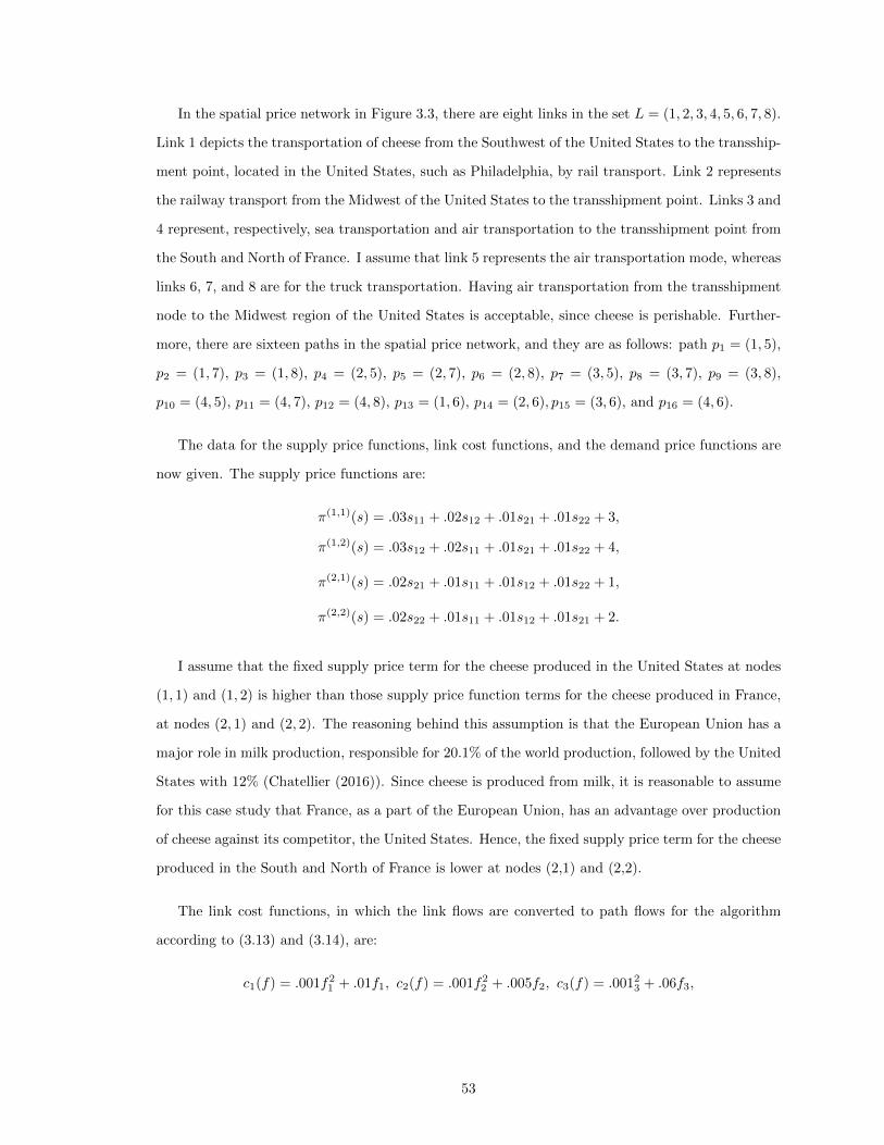
In the spatial price network in Figure 3.3, there are eight links in the set L = (1, 2, 3, 4, 5, 6, 7, 8).
Link 1 depicts the transportation of cheese from the Southwest of the United States to the transship-
ment point, located in the United States, such as Philadelphia, by rail transport. Link 2 represents
the railway transport from the Midwest of the United States to the transshipment point. Links 3 and
4 represent, respectively, sea transportation and air transportation to the transshipment point from
the South and North of France. I assume that link 5 represents the air transportation mode, whereas
links 6, 7, and 8 are for the truck transportation. Having air transportation from the transshipment
node to the Midwest region of the United States is acceptable, since cheese is perishable. Further-
more, there are sixteen paths in the spatial price network, and they are as follows: path p1 = (1, 5),
p2 = (1, 7), p3 = (1, 8), p4 = (2, 5), p5 = (2, 7), p6 = (2, 8), p7 = (3, 5), p8 = (3, 7), p9 = (3, 8),
p10 = (4, 5), p11 = (4, 7), p12 = (4, 8), p13 = (1, 6), p14 = (2, 6), p15 = (3, 6), and p16 = (4, 6).
The data for the supply price functions, link cost functions, and the demand price functions are
now given. The supply price functions are:
π(1,1)(s) = .03s11 + .02s12 + .01s21 + .01s22 + 3,
π(1,2)(s) = .03s12 + .02s11 + .01s21 + .01s22 + 4,
π(2,1)(s) = .02s21 + .01s11 + .01s12 + .01s22 + 1,
π(2,2)(s) = .02s22 + .01s11 + .01s12 + .01s21 + 2.
I assume that the fixed supply price term for the cheese produced in the United States at nodes
(1, 1) and (1, 2) is higher than those supply price function terms for the cheese produced in France,
at nodes (2, 1) and (2, 2). The reasoning behind this assumption is that the European Union has a
major role in milk production, responsible for 20.1% of the world production, followed by the United
States with 12% (Chatellier (2016)). Since cheese is produced from milk, it is reasonable to assume
for this case study that France, as a part of the European Union, has an advantage over production
of cheese against its competitor, the United States. Hence, the fixed supply price term for the cheese
produced in the South and North of France is lower at nodes (2,1) and (2,2).
The link cost functions, in which the link flows are converted to path flows for the algorithm
according to (3.13) and (3.14), are:
c1(f) = .001f21 + .01f1, c2(f) = .001f22 + .005f2, c3(f) = .00123 + .06f3,
53
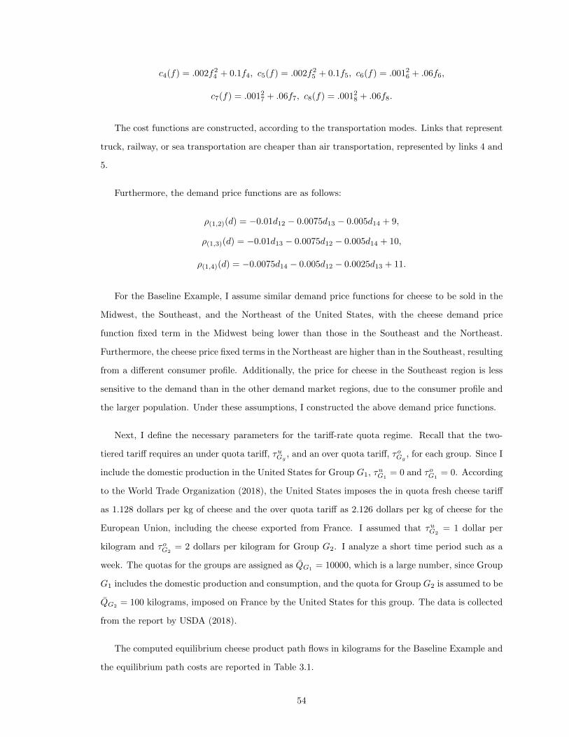
c4(f) = .002f24 + 0.1f4, c5(f) = .002f25 + 0.1f5, c6(f) = .00126 + .06f6,
c7(f) = .00127 + .06f7, c8(f) = .00128 + .06f8.
The cost functions are constructed, according to the transportation modes. Links that represent
truck, railway, or sea transportation are cheaper than air transportation, represented by links 4 and
5.
Furthermore, the demand price functions are as follows:
ρ(1,2)(d) = −0.01d12 − 0.0075d13 − 0.005d14 + 9,
ρ(1,3)(d) = −0.01d13 − 0.0075d12 − 0.005d14 + 10,
ρ(1,4)(d) = −0.0075d14 − 0.005d12 − 0.0025d13 + 11.
For the Baseline Example, I assume similar demand price functions for cheese to be sold in the
Midwest, the Southeast, and the Northeast of the United States, with the cheese demand price
function fixed term in the Midwest being lower than those in the Southeast and the Northeast.
Furthermore, the cheese price fixed terms in the Northeast are higher than in the Southeast, resulting
from a different consumer profile. Additionally, the price for cheese in the Southeast region is less
sensitive to the demand than in the other demand market regions, due to the consumer profile and
the larger population. Under these assumptions, I constructed the above demand price functions.
Next, I define the necessary parameters for the tariff-rate quota regime. Recall that the two-
tiered tariff requires an under quota tariff, τuGg, and an over quota tariff, τoGg
, for each group. Since I
include the domestic production in the United States for Group G1, τuG1= 0 and τoG1
= 0. According
to the World Trade Organization (2018), the United States imposes the in quota fresh cheese tariff
as 1.128 dollars per kg of cheese and the over quota tariff as 2.126 dollars per kg of cheese for the
European Union, including the cheese exported from France. I assumed that τuG2= 1 dollar per
kilogram and τoG2= 2 dollars per kilogram for Group G2. I analyze a short time period such as a
week. The quotas for the groups are assigned as QG1= 10000, which is a large number, since Group
G1 includes the domestic production and consumption, and the quota for Group G2 is assumed to be
QG2 = 100 kilograms, imposed on France by the United States for this group. The data is collected
from the report by USDA (2018).
The computed equilibrium cheese product path flows in kilograms for the Baseline Example and
the equilibrium path costs are reported in Table 3.1.
54
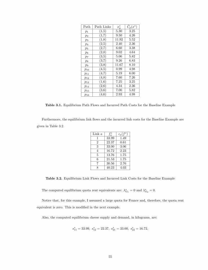
Path Path Links x∗p Cp(x∗)
p1 (1,5) 5.30 3.25p2 (1,7) 9.50 4.26p3 (1,8) 11.92 5.52p4 (2,5) 2.40 2.36p5 (2,7) 6.60 3.38p6 (2,8) 9.02 4.64p7 (3,5) 5.06 5.82p8 (3,7) 9.26 6.83p9 (3,8) 11.67 8.10p10 (4,5) 0.99 4.98p11 (4,7) 5.19 6.00p12 (4,8) 7.60 7.26p13 (1,6) 7.25 3.25p14 (2,6) 4.34 2.36p15 (3,6) 7.00 5.82p16 (4,6) 2.93 4.98
Table 3.1. Equilibrium Path Flows and Incurred Path Costs for the Baseline Example
Furthermore, the equilibrium link flows and the incurred link costs for the Baseline Example are
given in Table 3.2.
Link a f∗a ca(f∗)1 33.99 1.492 22.37 0.613 33.00 3.064 16.72 2.235 13.76 1.756 21.53 1.757 30.56 2.768 40.23 4.03
Table 3.2. Equilibrium Link Flows and Incurred Link Costs for the Baseline Example
The computed equilibrium quota rent equivalents are: λ∗G1= 0 and λ∗G2
= 0.
Notice that, for this example, I assumed a large quota for France and, therefore, the quota rent
equivalent is zero. This is modified in the next example.
Also, the computed equilibrium cheese supply and demand, in kilograms, are:
s∗11 = 33.99, s∗12 = 22.37, s∗21 = 33.00, s∗22 = 16.72,
55
d∗12 = 35.30, d∗13 = 30.56, d∗14 = 40.23.
The total amount of cheese shipment from the Southwest and Midwest regions of the United
States is larger than the cheese shipments from the South and North of France.
Furthermore, the incurred supply prices per kilogram of cheese in dollars are:
π(1,1) = 4.96, π(1,2) = 5.84, π(2,1) = 2.39, π(2,2) = 3.22.
Observe that the supply prices of cheese are higher in the Southwest and the Midwest regions
of the United States than in the South and North regions of France. This should have given an
advantage to France to export their cheese in a larger amount to the United States; however, since
the transportation costs are larger for France, and their cheese is also subject to an under tariff of
τuG2= 1 (cf. (3.9) and (3.10)) large export amounts are not achieved.
Next, I report the incurred demand prices, per kilogram of cheese, at the equilibrium, in dollars:
ρ(1,2) = 8.21, ρ(1,3) = 9.22, ρ(1,4) = 10.49.
The demand price for cheese in the Southeast of the US is higher than it is in the Northeast.
This is reasonable due to the demographic differences in these demand regions.
The equilibrium conditions (3.9) and (3.10) are satisfied with excellent accuracy.
3.5.2 Change in Quotas Example
This example is constructed from the Baseline Example and has the spatial price network topol-
ogy in Figure 3.3 as well as the same data, except for the following. In this example, I decrease
the quota of Group G2. In 2018, the turmoil in world trade generated an environment in which
the import countries started to modify their tariffs and tariff-rate quotas to maintain their political
agendas (cf. Paquette, Lynch, and Rauhala (2018)). In a broader sense, import countries can impose
stricter quotas and higher under quota and over quota tariffs on their trade partners to support their
domestic production. I, hence, modify the tariffs and quotas to investigate the associated impacts
on the economy.
For the Change in Quotas Example, I consider the situation in which the United States imposes
a stricter quota on cheese that is exported from France’s supply regions. Therefore, the quota on
56
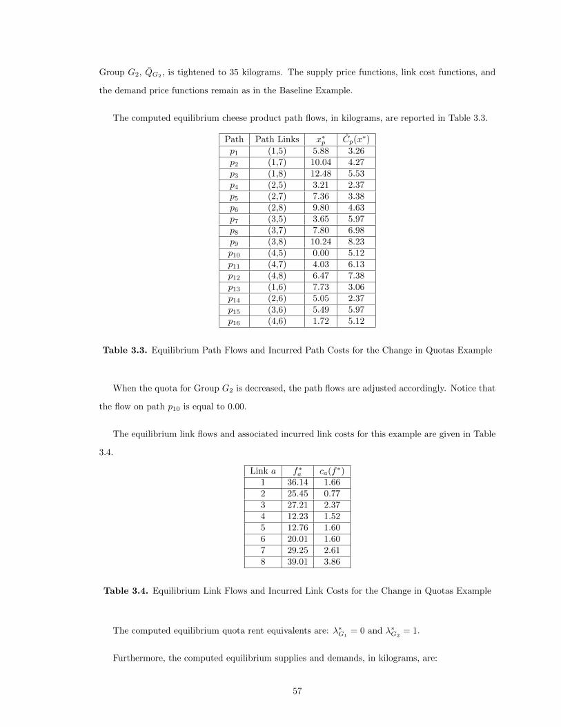
Group G2, QG2 , is tightened to 35 kilograms. The supply price functions, link cost functions, and
the demand price functions remain as in the Baseline Example.
The computed equilibrium cheese product path flows, in kilograms, are reported in Table 3.3.
Path Path Links x∗p Cp(x∗)
p1 (1,5) 5.88 3.26p2 (1,7) 10.04 4.27p3 (1,8) 12.48 5.53p4 (2,5) 3.21 2.37p5 (2,7) 7.36 3.38p6 (2,8) 9.80 4.63p7 (3,5) 3.65 5.97p8 (3,7) 7.80 6.98p9 (3,8) 10.24 8.23p10 (4,5) 0.00 5.12p11 (4,7) 4.03 6.13p12 (4,8) 6.47 7.38p13 (1,6) 7.73 3.06p14 (2,6) 5.05 2.37p15 (3,6) 5.49 5.97p16 (4,6) 1.72 5.12
Table 3.3. Equilibrium Path Flows and Incurred Path Costs for the Change in Quotas Example
When the quota for Group G2 is decreased, the path flows are adjusted accordingly. Notice that
the flow on path p10 is equal to 0.00.
The equilibrium link flows and associated incurred link costs for this example are given in Table
3.4.
Link a f∗a ca(f∗)1 36.14 1.662 25.45 0.773 27.21 2.374 12.23 1.525 12.76 1.606 20.01 1.607 29.25 2.618 39.01 3.86
Table 3.4. Equilibrium Link Flows and Incurred Link Costs for the Change in Quotas Example
The computed equilibrium quota rent equivalents are: λ∗G1= 0 and λ∗G2
= 1.
Furthermore, the computed equilibrium supplies and demands, in kilograms, are:
57
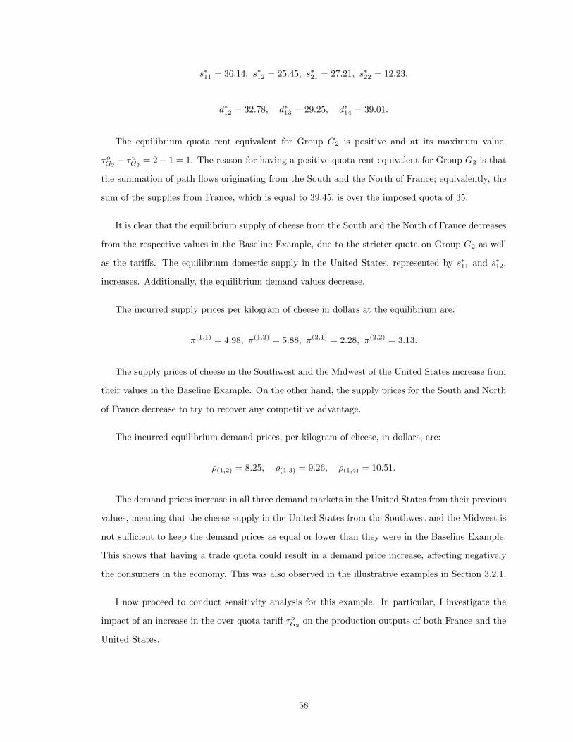
s∗11 = 36.14, s∗12 = 25.45, s∗21 = 27.21, s∗22 = 12.23,
d∗12 = 32.78, d∗13 = 29.25, d∗14 = 39.01.
The equilibrium quota rent equivalent for Group G2 is positive and at its maximum value,
τoG2− τuG2
= 2− 1 = 1. The reason for having a positive quota rent equivalent for Group G2 is that
the summation of path flows originating from the South and the North of France; equivalently, the
sum of the supplies from France, which is equal to 39.45, is over the imposed quota of 35.
It is clear that the equilibrium supply of cheese from the South and the North of France decreases
from the respective values in the Baseline Example, due to the stricter quota on Group G2 as well
as the tariffs. The equilibrium domestic supply in the United States, represented by s∗11 and s∗12,
increases. Additionally, the equilibrium demand values decrease.
The incurred supply prices per kilogram of cheese in dollars at the equilibrium are:
π(1,1) = 4.98, π(1,2) = 5.88, π(2,1) = 2.28, π(2,2) = 3.13.
The supply prices of cheese in the Southwest and the Midwest of the United States increase from
their values in the Baseline Example. On the other hand, the supply prices for the South and North
of France decrease to try to recover any competitive advantage.
The incurred equilibrium demand prices, per kilogram of cheese, in dollars, are:
ρ(1,2) = 8.25, ρ(1,3) = 9.26, ρ(1,4) = 10.51.
The demand prices increase in all three demand markets in the United States from their previous
values, meaning that the cheese supply in the United States from the Southwest and the Midwest is
not sufficient to keep the demand prices as equal or lower than they were in the Baseline Example.
This shows that having a trade quota could result in a demand price increase, affecting negatively
the consumers in the economy. This was also observed in the illustrative examples in Section 3.2.1.
I now proceed to conduct sensitivity analysis for this example. In particular, I investigate the
impact of an increase in the over quota tariff τoG2on the production outputs of both France and the
United States.
58
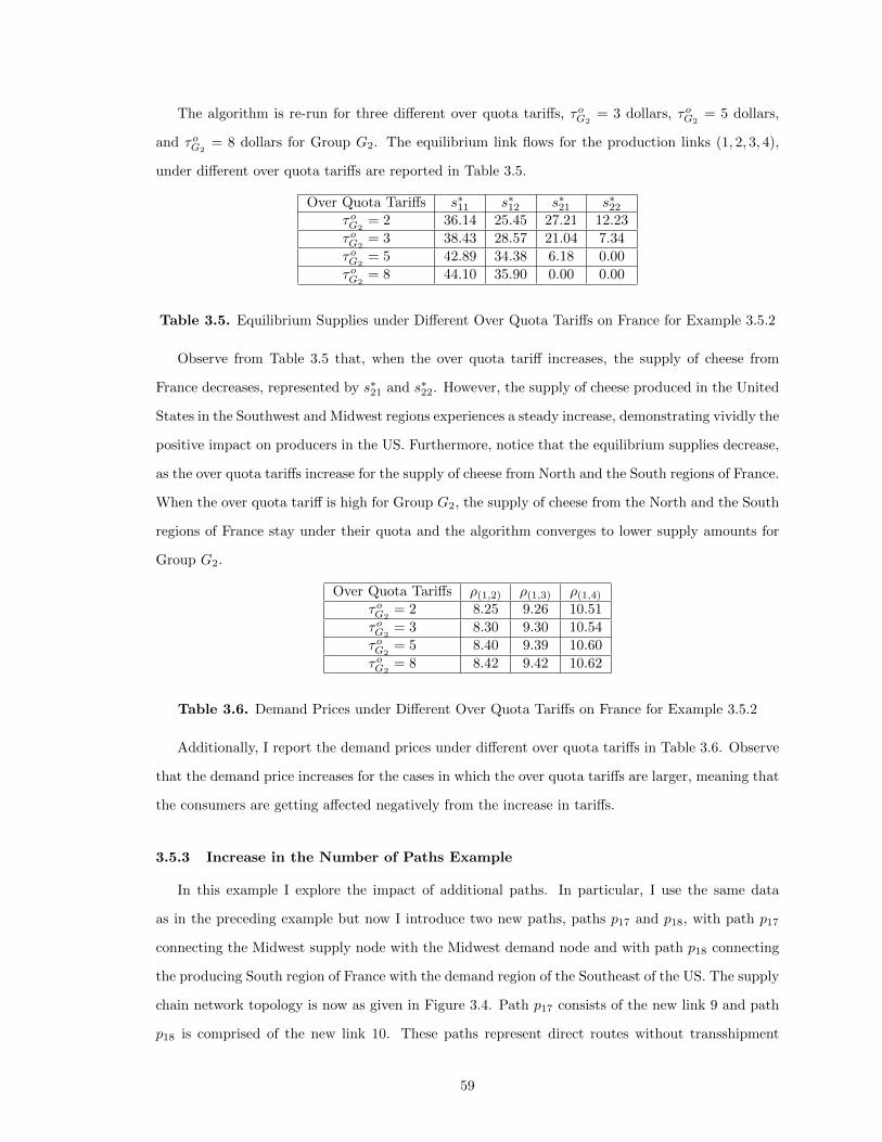
The algorithm is re-run for three different over quota tariffs, τoG2= 3 dollars, τoG2
= 5 dollars,
and τoG2= 8 dollars for Group G2. The equilibrium link flows for the production links (1, 2, 3, 4),
under different over quota tariffs are reported in Table 3.5.
Over Quota Tariffs s∗11 s∗12 s∗21 s∗22τoG2
= 2 36.14 25.45 27.21 12.23
τoG2= 3 38.43 28.57 21.04 7.34
τoG2= 5 42.89 34.38 6.18 0.00
τoG2= 8 44.10 35.90 0.00 0.00
Table 3.5. Equilibrium Supplies under Different Over Quota Tariffs on France for Example 3.5.2
Observe from Table 3.5 that, when the over quota tariff increases, the supply of cheese from
France decreases, represented by s∗21 and s∗22. However, the supply of cheese produced in the United
States in the Southwest and Midwest regions experiences a steady increase, demonstrating vividly the
positive impact on producers in the US. Furthermore, notice that the equilibrium supplies decrease,
as the over quota tariffs increase for the supply of cheese from North and the South regions of France.
When the over quota tariff is high for Group G2, the supply of cheese from the North and the South
regions of France stay under their quota and the algorithm converges to lower supply amounts for
Group G2.
Over Quota Tariffs ρ(1,2) ρ(1,3) ρ(1,4)τoG2
= 2 8.25 9.26 10.51
τoG2= 3 8.30 9.30 10.54
τoG2= 5 8.40 9.39 10.60
τoG2= 8 8.42 9.42 10.62
Table 3.6. Demand Prices under Different Over Quota Tariffs on France for Example 3.5.2
Additionally, I report the demand prices under different over quota tariffs in Table 3.6. Observe
that the demand price increases for the cases in which the over quota tariffs are larger, meaning that
the consumers are getting affected negatively from the increase in tariffs.
3.5.3 Increase in the Number of Paths Example
In this example I explore the impact of additional paths. In particular, I use the same data
as in the preceding example but now I introduce two new paths, paths p17 and p18, with path p17
connecting the Midwest supply node with the Midwest demand node and with path p18 connecting
the producing South region of France with the demand region of the Southeast of the US. The supply
chain network topology is now as given in Figure 3.4. Path p17 consists of the new link 9 and path
p18 is comprised of the new link 10. These paths represent direct routes without transshipment
59
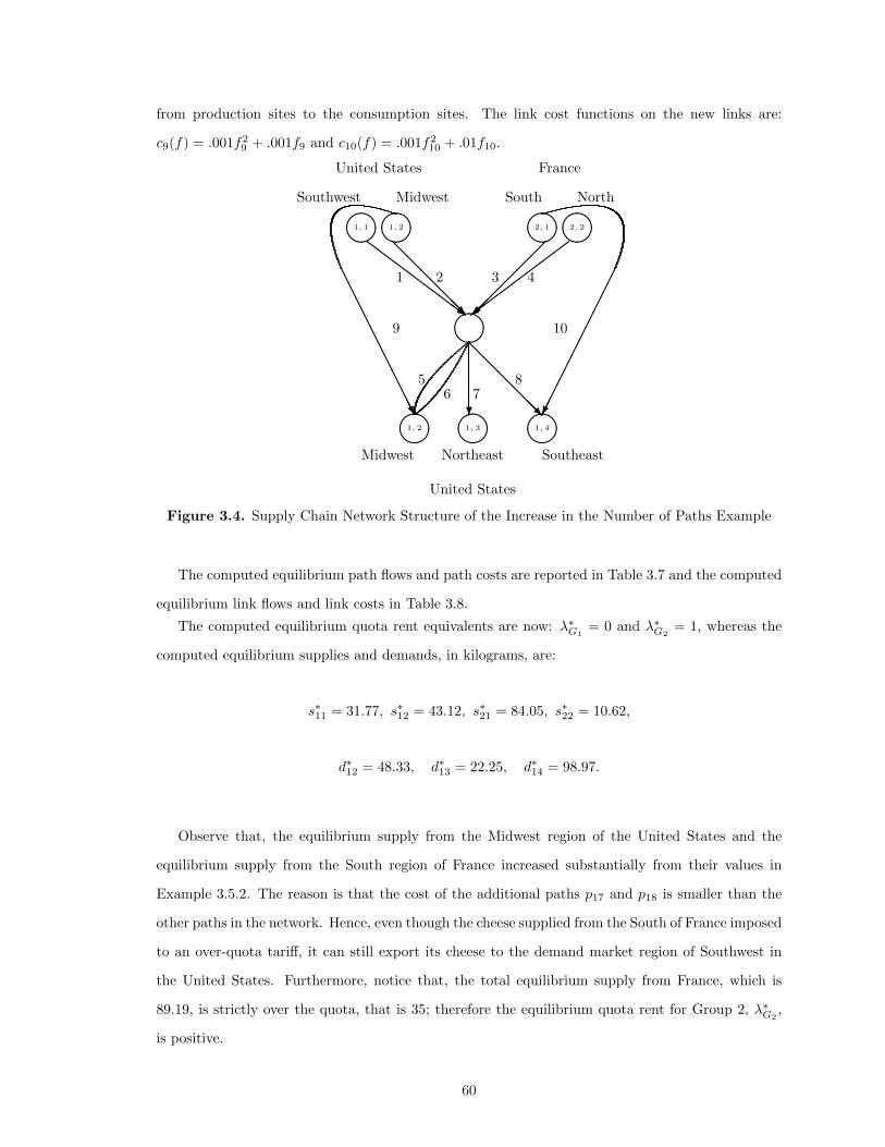
from production sites to the consumption sites. The link cost functions on the new links are:
c9(f) = .001f29 + .001f9 and c10(f) = .001f210 + .01f10.
����1, 1 ����1, 2
1 2 3 4
56 7
8
9 10
United States
Southwest Midwest
France
South North
����2, 1 ����2, 2
����
����1, 2 ����1, 3 ����1, 4
@@@@@@R?
��
����
��
��
���=
@@@@@@R
ZZZZZZZ~
Midwest Northeast Southeast
United States
AAAAAAAAAAAU
������������
Figure 3.4. Supply Chain Network Structure of the Increase in the Number of Paths Example
The computed equilibrium path flows and path costs are reported in Table 3.7 and the computed
equilibrium link flows and link costs in Table 3.8.
The computed equilibrium quota rent equivalents are now: λ∗G1= 0 and λ∗G2
= 1, whereas the
computed equilibrium supplies and demands, in kilograms, are:
s∗11 = 31.77, s∗12 = 43.12, s∗21 = 84.05, s∗22 = 10.62,
d∗12 = 48.33, d∗13 = 22.25, d∗14 = 98.97.
Observe that, the equilibrium supply from the Midwest region of the United States and the
equilibrium supply from the South region of France increased substantially from their values in
Example 3.5.2. The reason is that the cost of the additional paths p17 and p18 is smaller than the
other paths in the network. Hence, even though the cheese supplied from the South of France imposed
to an over-quota tariff, it can still export its cheese to the demand market region of Southwest in
the United States. Furthermore, notice that, the total equilibrium supply from France, which is
89.19, is strictly over the quota, that is 35; therefore the equilibrium quota rent for Group 2, λ∗G2,
is positive.
60
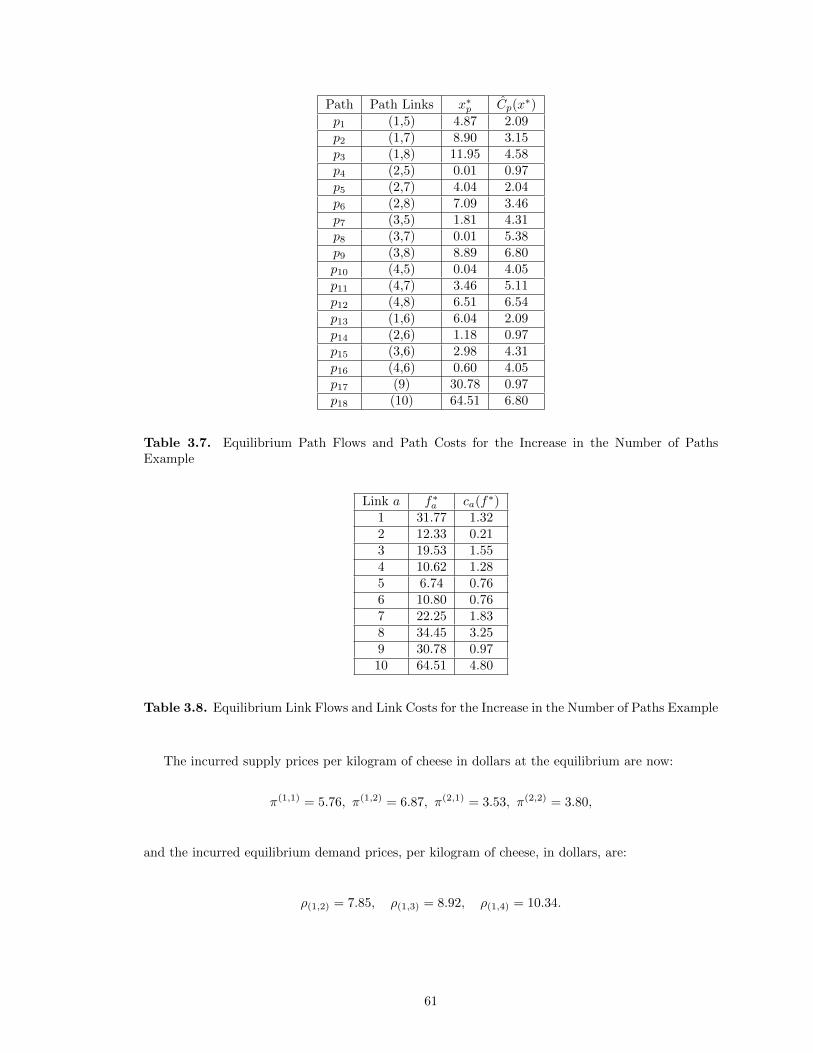
Path Path Links x∗p Cp(x∗)
p1 (1,5) 4.87 2.09p2 (1,7) 8.90 3.15p3 (1,8) 11.95 4.58p4 (2,5) 0.01 0.97p5 (2,7) 4.04 2.04p6 (2,8) 7.09 3.46p7 (3,5) 1.81 4.31p8 (3,7) 0.01 5.38p9 (3,8) 8.89 6.80p10 (4,5) 0.04 4.05p11 (4,7) 3.46 5.11p12 (4,8) 6.51 6.54p13 (1,6) 6.04 2.09p14 (2,6) 1.18 0.97p15 (3,6) 2.98 4.31p16 (4,6) 0.60 4.05p17 (9) 30.78 0.97p18 (10) 64.51 6.80
Table 3.7. Equilibrium Path Flows and Path Costs for the Increase in the Number of PathsExample
Link a f∗a ca(f∗)1 31.77 1.322 12.33 0.213 19.53 1.554 10.62 1.285 6.74 0.766 10.80 0.767 22.25 1.838 34.45 3.259 30.78 0.9710 64.51 4.80
Table 3.8. Equilibrium Link Flows and Link Costs for the Increase in the Number of Paths Example
The incurred supply prices per kilogram of cheese in dollars at the equilibrium are now:
π(1,1) = 5.76, π(1,2) = 6.87, π(2,1) = 3.53, π(2,2) = 3.80,
and the incurred equilibrium demand prices, per kilogram of cheese, in dollars, are:
ρ(1,2) = 7.85, ρ(1,3) = 8.92, ρ(1,4) = 10.34.
61
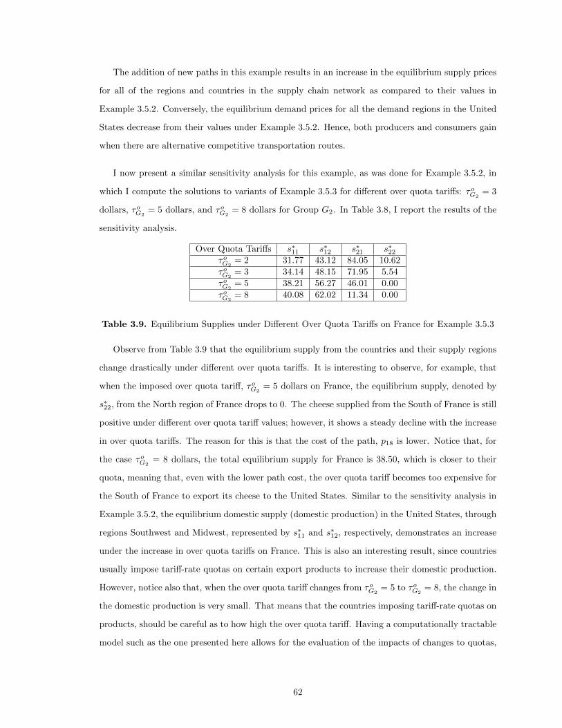
The addition of new paths in this example results in an increase in the equilibrium supply prices
for all of the regions and countries in the supply chain network as compared to their values in
Example 3.5.2. Conversely, the equilibrium demand prices for all the demand regions in the United
States decrease from their values under Example 3.5.2. Hence, both producers and consumers gain
when there are alternative competitive transportation routes.
I now present a similar sensitivity analysis for this example, as was done for Example 3.5.2, in
which I compute the solutions to variants of Example 3.5.3 for different over quota tariffs: τoG2= 3
dollars, τoG2= 5 dollars, and τoG2
= 8 dollars for Group G2. In Table 3.8, I report the results of the
sensitivity analysis.
Over Quota Tariffs s∗11 s∗12 s∗21 s∗22τoG2
= 2 31.77 43.12 84.05 10.62
τoG2= 3 34.14 48.15 71.95 5.54
τoG2= 5 38.21 56.27 46.01 0.00
τoG2= 8 40.08 62.02 11.34 0.00
Table 3.9. Equilibrium Supplies under Different Over Quota Tariffs on France for Example 3.5.3
Observe from Table 3.9 that the equilibrium supply from the countries and their supply regions
change drastically under different over quota tariffs. It is interesting to observe, for example, that
when the imposed over quota tariff, τoG2= 5 dollars on France, the equilibrium supply, denoted by
s∗22, from the North region of France drops to 0. The cheese supplied from the South of France is still
positive under different over quota tariff values; however, it shows a steady decline with the increase
in over quota tariffs. The reason for this is that the cost of the path, p18 is lower. Notice that, for
the case τoG2= 8 dollars, the total equilibrium supply for France is 38.50, which is closer to their
quota, meaning that, even with the lower path cost, the over quota tariff becomes too expensive for
the South of France to export its cheese to the United States. Similar to the sensitivity analysis in
Example 3.5.2, the equilibrium domestic supply (domestic production) in the United States, through
regions Southwest and Midwest, represented by s∗11 and s∗12, respectively, demonstrates an increase
under the increase in over quota tariffs on France. This is also an interesting result, since countries
usually impose tariff-rate quotas on certain export products to increase their domestic production.
However, notice also that, when the over quota tariff changes from τoG2= 5 to τoG2
= 8, the change in
the domestic production is very small. That means that the countries imposing tariff-rate quotas on
products, should be careful as to how high the over quota tariff. Having a computationally tractable
model such as the one presented here allows for the evaluation of the impacts of changes to quotas,
62
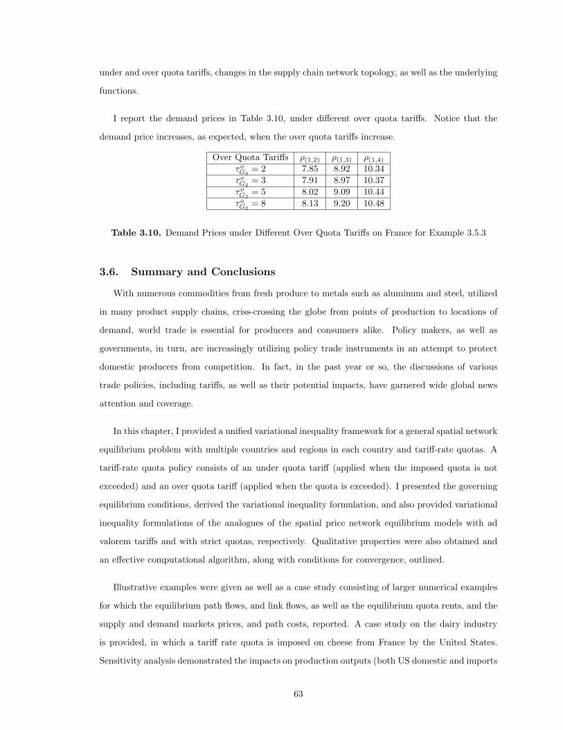
under and over quota tariffs, changes in the supply chain network topology, as well as the underlying
functions.
I report the demand prices in Table 3.10, under different over quota tariffs. Notice that the
demand price increases, as expected, when the over quota tariffs increase.
Over Quota Tariffs ρ(1,2) ρ(1,3) ρ(1,4)τoG2
= 2 7.85 8.92 10.34
τoG2= 3 7.91 8.97 10.37
τoG2= 5 8.02 9.09 10.44
τoG2= 8 8.13 9.20 10.48
Table 3.10. Demand Prices under Different Over Quota Tariffs on France for Example 3.5.3
3.6. Summary and Conclusions
With numerous commodities from fresh produce to metals such as aluminum and steel, utilized
in many product supply chains, criss-crossing the globe from points of production to locations of
demand, world trade is essential for producers and consumers alike. Policy makers, as well as
governments, in turn, are increasingly utilizing policy trade instruments in an attempt to protect
domestic producers from competition. In fact, in the past year or so, the discussions of various
trade policies, including tariffs, as well as their potential impacts, have garnered wide global news
attention and coverage.
In this chapter, I provided a unified variational inequality framework for a general spatial network
equilibrium problem with multiple countries and regions in each country and tariff-rate quotas. A
tariff-rate quota policy consists of an under quota tariff (applied when the imposed quota is not
exceeded) and an over quota tariff (applied when the quota is exceeded). I presented the governing
equilibrium conditions, derived the variational inequality formulation, and also provided variational
inequality formulations of the analogues of the spatial price network equilibrium models with ad
valorem tariffs and with strict quotas, respectively. Qualitative properties were also obtained and
an effective computational algorithm, along with conditions for convergence, outlined.
Illustrative examples were given as well as a case study consisting of larger numerical examples
for which the equilibrium path flows, and link flows, as well as the equilibrium quota rents, and the
supply and demand markets prices, and path costs, reported. A case study on the dairy industry
is provided, in which a tariff rate quota is imposed on cheese from France by the United States.
Sensitivity analysis demonstrated the impacts on production outputs (both US domestic and imports
63
from France) of a tightening of the imposed quota as well as increases in the over tariff rate. The
results showed that while domestic producers are protected by tariff rate quotas, the consumers
suffer.
64
CHAPTER 4
STRICT QUOTAS OR TARIFFS? IMPLICATIONS FOR PRODUCTQUALITY AND CONSUMER WELFARE IN DIFFERENTIATED
PRODUCT SUPPLY CHAINS
In this chapter, I present a differentiated product supply chain network equilibrium model with
quality and trade instruments, which is based on the paper by Nagurney, Besik, and Li (2019).
Chapter 4 is organized as follows. In Section 4.1, I first present the differentiated product supply
chain network equilibrium model with quality, but without trade policy instruments in the form of a
tariff or quota. The model generalizes the model introduced in Nagurney and Li (2014) in that the
demand price functions are differentiated by producing firm. I state the governing Nash equilibrium
conditions and provide the variational inequality formulation.
I also provide constructs for quantifying consumer welfare in the presence or absence of tariffs
or quotas in differentiated product supply chain networks with quality. Through simple illustrative
examples in Section 4.1, I show that the imposition of a tariff or quota may adversely affect both
the quality of products as well as the consumer welfare.
In Section 4.2, I propose the algorithm, which is then applied in Section 4.3 to a series of
numerical examples, accompanied by sensitivity analysis, comprising a case study focused on the
agricultural product of soybeans. The case study explores the impacts of the imposition of a strict
quota or a tariff by China on soybeans that are produced in the United States on equilibrium soybean
flows, product quality, prices, firm profits, and consumer welfare. Multiple scenarios are generated,
including a disruption at a production side, as well as the addition of a demand market. The case
study yields interesting results for decision-makers and policy makers.
In Sections 4.4 and 4.5, I summarize the results, and present conclusions.
65
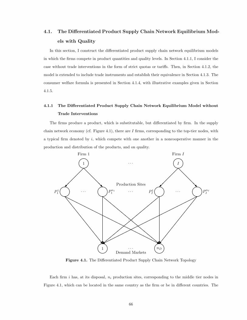
4.1. The Differentiated Product Supply Chain Network Equilibrium Mod-
els with Quality
In this section, I construct the differentiated product supply chain network equilibrium models
in which the firms compete in product quantities and quality levels. In Section 4.1.1, I consider the
case without trade interventions in the form of strict quotas or tariffs. Then, in Section 4.1.2, the
model is extended to include trade instruments and establish their equivalence in Section 4.1.3. The
consumer welfare formula is presented in Section 4.1.4, with illustrative examples given in Section
4.1.5.
4.1.1 The Differentiated Product Supply Chain Network Equilibrium Model without
Trade Interventions
The firms produce a product, which is substitutable, but differentiated by firm. In the supply
chain network economy (cf. Figure 4.1), there are I firms, corresponding to the top-tier nodes, with
a typical firm denoted by i, which compete with one another in a noncooperative manner in the
production and distribution of the products, and on quality.
����
1 · · · nD����
Demand Markets
P 11����
· · · ����
Pn11 · · ·
Production Sites
P 1I����
· · · ����
PnI
I
��
���
@@@@@R
��
���
@@@@@R
����
1 ����I· · ·
Firm 1 Firm I
\\\\\\\\\\\\
HHHHHHHHHHHHHHHHHHHHHHHH
lllllllllllllll
· · ·
������������
,,,,,,,,,,,,,,,
������������������������ ??� RjR
Figure 4.1. The Differentiated Product Supply Chain Network Topology
Each firm i has, at its disposal, ni production sites, corresponding to the middle tier nodes in
Figure 4.1, which can be located in the same country as the firm or be in different countries. The
66
production sites of firm i at the middle tier are denoted by P 1i , . . . , P
nii , respectively, with a typical
such site denoted by P ji . The firms determine the quantities to produce at each of their sites which
are then transported to the nD demand markets, corresponding to the bottom nodes in Figure 4.1.
A typical demand market is denoted, without loss of generality, by k; k = 1, . . . , nD. In addition,
the firms must determine the quality level of the product at each of their production sites, which can
differ from site to site. Consumers, located at the demand markets, signal their preferences through
the prices that they are willing to pay for the products, which are differentiated by firm (although
they are substitutes), and, since a firm’s product may be produced at one or more sites, a firm’s
product at a demand market is characterized by its average quality. It is assumed that the quality
is preserved (with an associated cost) in the distribution process.
A link in Figure 4.1 joining a firm node with one of its production site nodes corresponds to the
production/manufacturing activity, whereas a link joining a production site node with a demand
market node corresponds to the activity of distribution. Note that, in the case of agricultural
production, production sites would correspond to farms.
The notation for the model is given in Table 4.1.
The production output at firm i’s production site P ji and the demand for the product at each
demand market k must satisfy, respectively, the conservation of flow equations (4.1) and (4.2):
sij =
nD∑k=1
Qijk, i = 1, . . . , I; j = 1, . . . , ni, (4.1)
dik =
ni∑j=1
Qijk, k = 1, . . . , nD. (4.2)
According to (4.1), the output produced at a firm’s production site is equal to the sum of the
product amounts distributed to the demand markets from that site, and, according to (4.2), the
quantity of a product produced by a firm and consumed at a demand market is equal to the sum of
the amounts shipped by the firm from its production sites to that demand market.
In addition, the product shipments must be nonnegative, that is:
Qijk ≥ 0, i = 1, . . . , I; j = 1, . . . , ni; k = 1, . . . , nD. (4.3)
The quality levels, in turn, must meet or exceed the nonnegative minimum quality standards
(MQSs) at the production sites, but they cannot exceed their respective upper bounds of quality:
67
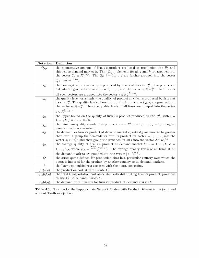
Notation Definition
Qijk the nonnegative amount of firm i’s product produced at production site P ji andshipped to demand market k. The {Qijk} elements for all j and k are grouped intothe vector Qi ∈ RninD
+ . The Qi; i = 1, . . . , I are further grouped into the vector
Q ∈ R∑I
i=1 ninD
+ .
sij the nonnegative product output produced by firm i at its site P ji . The productionoutputs are grouped for each i; i = 1, . . . , I, into the vector si ∈ Rni
+ . Then further
all such vectors are grouped into the vector s ∈ R∑I
i=1 ni
+ .qij the quality level, or, simply, the quality, of product i, which is produced by firm i at
its site P ji . The quality levels of each firm i; i = 1, . . . , I, the {qij}, are grouped intothe vector qi ∈ Rni
+ . Then the quality levels of all firms are grouped into the vector
q ∈ R∑I
i=1 ni
+ .
qij the upper bound on the quality of firm i’s product produced at site P ji , with i =1, . . . , I; j = 1, . . . , ni,∀i.
qij
the minimum quality standard at production site P ji ; i = 1, . . . , I; j = 1, . . . , ni,∀i,assumed to be nonnegative.
dik the demand for firm i’s product at demand market k, with dik assumed to be greaterthan zero. I group the demands for firm i’s product for each i = 1, . . . , I, into thevector di ∈ RnD
+ and then group the demands for all i into the vector d ∈ RInD+ .
qik the average quality of firm i’s product at demand market k; i = 1, . . . , I; k =
1, . . . , nD, where qik =∑ni
j=1 qijQijk
dik. The average quality levels of all firms at all
the demand markets are grouped into the vector q ∈ RInD+ .
Q the strict quota defined for production sites in a particular country over which thequota is imposed for the product by another country to its demand markets.
λ the Lagrange multiplier associated with the quota constraint.
fij(s, q) the production cost at firm i’s site P ji .cijk(Q, q) the total transportation cost associated with distributing firm i’s product, produced
at site P ji , to demand market k.ρik(d, q) the demand price function for firm i’s product at demand market k.
Table 4.1. Notation for the Supply Chain Network Models with Product Differentiation (with andwithout Tariffs or Quotas)
68
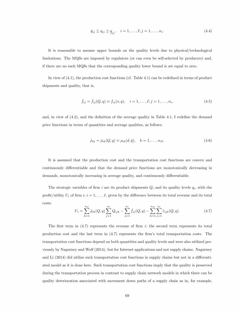
qij ≥ qij ≥ qij , i = 1, . . . , I; j = 1, . . . , ni. (4.4)
It is reasonable to assume upper bounds on the quality levels due to physical/technological
limitations. The MQSs are imposed by regulators (or can even be self-selected by producers) and,
if there are no such MQSs that the corresponding quality lower bound is set equal to zero.
In view of (4.1), the production cost functions (cf. Table 4.1) can be redefined in terms of product
shipments and quality, that is,
fij = fij(Q, q) ≡ fij(s, q), i = 1, . . . , I; j = 1, . . . , ni, (4.5)
and, in view of (4.2), and the definition of the average quality in Table 4.1, I redefine the demand
price functions in terms of quantities and average qualities, as follows:
ρik = ρik(Q, q) ≡ ρik(d, q), k = 1, . . . , nD. (4.6)
It is assumed that the production cost and the transportation cost functions are convex and
continuously differentiable and that the demand price functions are monotonically decreasing in
demands, monotonically increasing in average quality, and continuously differentiable.
The strategic variables of firm i are its product shipments Qi and its quality levels qi, with the
profit/utility Ui of firm i; i = 1, . . . , I, given by the difference between its total revenue and its total
costs:
Ui =
nD∑k=1
ρik(Q, q)
ni∑j=1
Qijk −ni∑j=1
fij(Q, q)−nD∑k=1
ni∑j=1
cijk(Q, q). (4.7)
The first term in (4.7) represents the revenue of firm i; the second term represents its total
production cost and the last term in (4.7) represents the firm’s total transportation costs. The
transportation cost functions depend on both quantities and quality levels and were also utilized pre-
viously by Nagurney and Wolf (2014), but for Internet applications and not supply chains. Nagurney
and Li (2014) did utilize such transportation cost functions in supply chains but not in a differenti-
ated model as it is done here. Such transportation cost functions imply that the quality is preserved
during the transportation process in contrast to supply chain network models in which there can be
quality deterioration associated with movement down paths of a supply chain as in, for example,
69
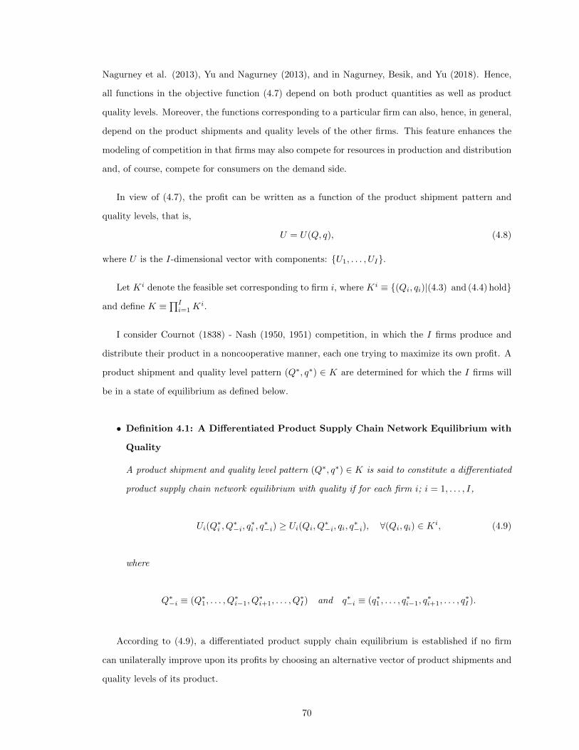
Nagurney et al. (2013), Yu and Nagurney (2013), and in Nagurney, Besik, and Yu (2018). Hence,
all functions in the objective function (4.7) depend on both product quantities as well as product
quality levels. Moreover, the functions corresponding to a particular firm can also, hence, in general,
depend on the product shipments and quality levels of the other firms. This feature enhances the
modeling of competition in that firms may also compete for resources in production and distribution
and, of course, compete for consumers on the demand side.
In view of (4.7), the profit can be written as a function of the product shipment pattern and
quality levels, that is,
U = U(Q, q), (4.8)
where U is the I-dimensional vector with components: {U1, . . . , UI}.
Let Ki denote the feasible set corresponding to firm i, where Ki ≡ {(Qi, qi)|(4.3) and (4.4) hold}
and define K ≡∏Ii=1K
i.
I consider Cournot (1838) - Nash (1950, 1951) competition, in which the I firms produce and
distribute their product in a noncooperative manner, each one trying to maximize its own profit. A
product shipment and quality level pattern (Q∗, q∗) ∈ K are determined for which the I firms will
be in a state of equilibrium as defined below.
• Definition 4.1: A Differentiated Product Supply Chain Network Equilibrium with
Quality
A product shipment and quality level pattern (Q∗, q∗) ∈ K is said to constitute a differentiated
product supply chain network equilibrium with quality if for each firm i; i = 1, . . . , I,
Ui(Q∗i , Q
∗−i, q
∗i , q∗−i) ≥ Ui(Qi, Q∗−i, qi, q∗−i), ∀(Qi, qi) ∈ Ki, (4.9)
where
Q∗−i ≡ (Q∗1, . . . , Q∗i−1, Q
∗i+1, . . . , Q
∗I) and q∗−i ≡ (q∗1 , . . . , q
∗i−1, q
∗i+1, . . . , q
∗I ).
According to (4.9), a differentiated product supply chain equilibrium is established if no firm
can unilaterally improve upon its profits by choosing an alternative vector of product shipments and
quality levels of its product.
70
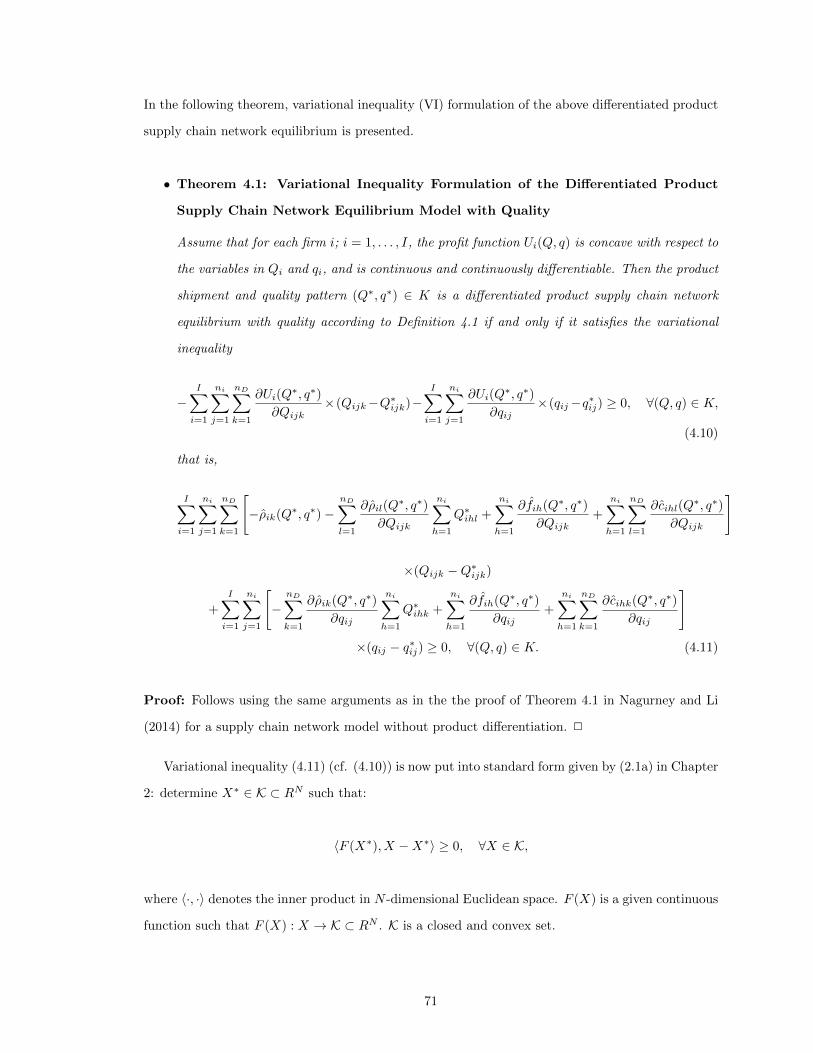
In the following theorem, variational inequality (VI) formulation of the above differentiated product
supply chain network equilibrium is presented.
• Theorem 4.1: Variational Inequality Formulation of the Differentiated Product
Supply Chain Network Equilibrium Model with Quality
Assume that for each firm i; i = 1, . . . , I, the profit function Ui(Q, q) is concave with respect to
the variables in Qi and qi, and is continuous and continuously differentiable. Then the product
shipment and quality pattern (Q∗, q∗) ∈ K is a differentiated product supply chain network
equilibrium with quality according to Definition 4.1 if and only if it satisfies the variational
inequality
−I∑i=1
ni∑j=1
nD∑k=1
∂Ui(Q∗, q∗)
∂Qijk×(Qijk−Q∗ijk)−
I∑i=1
ni∑j=1
∂Ui(Q∗, q∗)
∂qij×(qij−q∗ij) ≥ 0, ∀(Q, q) ∈ K,
(4.10)
that is,
I∑i=1
ni∑j=1
nD∑k=1
[−ρik(Q∗, q∗)−
nD∑l=1
∂ρil(Q∗, q∗)
∂Qijk
ni∑h=1
Q∗ihl +
ni∑h=1
∂fih(Q∗, q∗)
∂Qijk+
ni∑h=1
nD∑l=1
∂cihl(Q∗, q∗)
∂Qijk
]
×(Qijk −Q∗ijk)
+
I∑i=1
ni∑j=1
[−
nD∑k=1
∂ρik(Q∗, q∗)
∂qij
ni∑h=1
Q∗ihk +
ni∑h=1
∂fih(Q∗, q∗)
∂qij+
ni∑h=1
nD∑k=1
∂cihk(Q∗, q∗)
∂qij
]×(qij − q∗ij) ≥ 0, ∀(Q, q) ∈ K. (4.11)
Proof: Follows using the same arguments as in the the proof of Theorem 4.1 in Nagurney and Li
(2014) for a supply chain network model without product differentiation. 2
Variational inequality (4.11) (cf. (4.10)) is now put into standard form given by (2.1a) in Chapter
2: determine X∗ ∈ K ⊂ RN such that:
〈F (X∗), X −X∗〉 ≥ 0, ∀X ∈ K,
where 〈·, ·〉 denotes the inner product in N -dimensional Euclidean space. F (X) is a given continuous
function such that F (X) : X → K ⊂ RN . K is a closed and convex set.
71

For the differentiated product supply chain network equilibrium model without trade interven-
tions, I define X ≡ (Q, q) and F (X) ≡ (F 1(X), F 2(X)) with F 1ijk(X) ≡ −∂Ui(Q,q)
∂Qijk; i = 1, . . . , I; j =
1, . . . , ni; k = 1, . . . , nD, and F 2ij(X) ≡ −∂Ui(Q,q)
∂qij; i = 1, . . . , I; j = 1, . . . , ni. Also, I define the
feasible set K ≡ K, and let N = IninD + Ini. Then, variational inequality (4.11) (cf. (4.10)) can
be put into the above standard form.
For further background on the variational inequality problem and supply chain network problems,
I refer the reader to the books by Nagurney (2006) and Nagurney and Li (2016). I emphasize the
above model (even without the inclusion of any trade policies) generalizes the model of Nagurney
and Li (2014) in that the demand price functions are differentiated by producing firm; that is, the
consumers at a demand market display their preferences accordingly.
Using the supply chain network model in Section 4.1.1 as a basis, I now construct extensions
that incorporate trade instruments such as a strict quota or tariff.
4.1.2 The Differentiated Product Supply Chain Network Equilibrium Model with a
Strict Quota
I first consider the inclusion of a strict quota. Specifically, I consider a country imposing a strict
quota on the product flows from another country. The quota is denoted by Q and the production
sites {j} are grouped in the country on which the quota is imposed on into the set O and the demand
markets {k} in the country imposing the quota into the set D. I then define the group G consisting
of all these production site and demand market pairs (j, k).
Under a strict quota regime, the following additional constraint must be satisfied:
I∑i=1
∑(j,k)∈G
Qijk ≤ Q. (4.12)
Observe that constraint (4.12) is a common or shared constraint associated with firms having
production sites in the country on which the quota is imposed. Hence, the original feasible set K
applied in the model in Section 4.1.1 should be expanded. Hence, the set S is defined as:
S ≡ {Q|(4.12) holds}. (4.13)
72
Note that the utility function (4.7) of a firm i depends on not only its own strategies, but
also on those of the other firms, and now their feasible sets do as well since the new feasible set
will correspond to K ∩ S. Therefore, the governing equilibrium concept is no longer that of Nash
Equilibrium, as was the case for the model in Section 4.1.1, but, rather, is that of a Generalized
Nash Equilibrium (GNE).
• Definition 4.2: A Differentiated Product Supply Chain Generalized Nash Network
Equilibrium with Quality
A product shipment and quality level pattern (Q∗, q∗) ∈ K∩S is a differentiated product supply
chain Generalized Nash Network Equilibrium with quality if for each firm i; i = 1, . . . , I,
Ui(Q∗i , Q
∗−i, q
∗i , q∗−i) ≥ Ui(Qi, Q∗−i, qi, q∗−i), ∀(Qi, qi) ∈ Ki ∩ S. (4.14)
As noted in Nagurney et al. (2017), for a supply chain network problem but without quality
and in the absence of any trade instruments, a refinement of the Generalized Nash Equilibrium is
a variational equilibrium and it is a specific type of GNE (see Facchinei and Kanzow (2010) and
Kulkarni and Shanbhag (2012)). In particular, in a GNE defined by a variational equilibrium, the
Lagrange multipliers associated with the shared/coupling constraints are all the same. This implies
that the firms whose production sites are affected by the quota share a common perception of the
strict quota in order to respect it.
Specifically, the following definition is necessary:
• Definition 4.3: Variational Equilibrium
A vector (Q∗, q∗) ∈ K ∩S is said to be a variational equilibrium of the above Generalized Nash
Network Equilibrium if it is a solution of the variational inequality
−I∑i=1
ni∑j=1
nD∑k=1
∂Ui(Q∗, q∗)
∂Qijk× (Qijk −Q∗ijk)−
I∑i=1
ni∑j=1
∂Ui(Q∗, q∗)
∂qij× (qij − q∗ij) ≥ 0,
∀(Q, q) ∈ K ∩ S. (4.15)
A solution to variational inequality (4.15) is guaranteed to exist, under the assumption that the
demand for products would be finite, since then the feasible set K ∩S is compact, and the function
that enters the variational inequality (4.15) is continuous (cf. Chapter 2).
73
Moreover, with a variational inequality formulation of the supply chain network model with strict
quotas, one can avail themselves of algorithmic schemes which are more highly developed than those
for quasivariational inequalities (cf. Bensoussan and Lions (1978) and Baiocchi and Capelo (1984)),
which have been used as a formalism for GNEs (Facchinei and Kanzow (2010)).
I define a new feasible set K which consists of (Q, q) ∈ K and λ ∈ R1+. Now, a variational
inequality which utilizes a Lagrange multiplier λ associated with the strict quota constraint (4.12)
are provided. Utilizing the results in Nagurney (2018) and Gossler et al. (2019), the following
corollary is immediate.
• Corollary 4.1: Alternative Variational Inequality Formulation of the Differentiated
Product Supply Chain Network Equilibrium Model with Quality and a Strict
Quota
An equivalent variational inequality to (4.15) is: determine (Q∗, q∗, λ∗) ∈ K such that
−I∑i=1
∑(j,k) 6∈G
∂Ui(Q∗, q∗)
∂Qijk× (Qijk −Q∗ijk) +
I∑i=1
∑(j,k)∈G
(−∂Ui(Q∗, q∗)
∂Qijk+ λ∗)× (Qijk −Q∗ijk)
−I∑i=1
ni∑j=1
∂Ui(Q∗, q∗)
∂qij× (qij − q∗ij)
+(Q−I∑i=1
∑(j,k)∈G
Q∗ijk)× (λ− λ∗) ≥ 0, ∀(Q, q, λ) ∈ K. (4.16)
Observe that the variational inequality (4.16) is defined on a feasible set with special structure,
including box-type constraints, a feature that will yield closed form expressions for the product
flows, the quality levels, and the Lagrange multiplier, at each iteration of the algorithmic scheme
that I propose in the next section.
Now, variational inequality (4.16) is put into standard form (cf. Equation (2.1a)). For the
differentiated product supply chain network equilibrium model with a strict quota, define X ≡
(Q, q, λ) and F (X) ≡ (F 3(X), F 4(X), F 5(X), F 6(X)) with F 3ijk ≡ −
∂Ui(Q,q)∂Qijk
; i = 1, . . . , I; (j, k) 6∈ G,
F 4ijk(X) ≡ −∂Ui(Q,q)
∂Qijk+ λ; i = 1, . . . , I; (j, k) ∈ G, F 5
ij(X) ≡ −∂Ui(Q,q)∂qij
; i = 1, . . . , I; j = 1, . . . , ni, and
F 6(X) ≡ Q−∑Ii=1
∑(j,k)∈G Qijk. Also, I define the feasible set K ≡ K, and let N = IninD+Ini+1.
Then, variational inequality (4.16) can be put into the standard form (cf. Equation (2.1a))).
74
4.1.3 The Differentiated Product Supply Chain Network Equilibrium Model with a
Tariff
I now introduce the tariff model based on the model in Section 4.1.1. A group G is considered
as in the strict quota model in Section 4.1.2, but, rather than imposing a strict quota, a tariff τ∗ is
imposed on the production sites in the country subject to the trade policy instrument.
The utility functions Ui; i = 1, . . . , I, then take the form
Ui = Ui −I∑i=1
∑(j,k)∈G
τ∗Qijk, (4.17)
with Ui; i = 1, . . . , I, as in (4.7).
The definition of an equilibrium then follows according to (4.9) but with Ui substituted for the
Ui; i = 1, . . . , I. The following Theorem is immediate from Theorem 4.1:
• Theorem 4.2: Variational Inequality Formulation of the Differentiated Product
Model Supply Chain Network Equilibrium Model with Quality and a Tariff
Under the same assumptions as in Theorem 4.1, a product shipment and quality pattern
(Q∗, q∗) ∈ K is a differentiated product supply chain network equilibrium according to Def-
inition 4.1 with Ui replacing Ui for i = 1, . . . , I, if and only if it satisfies the variational
inequality:
−I∑i=1
∑(j,k)6∈G
∂Ui(Q∗, q∗)
∂Qijk× (Qijk −Q∗ijk) +
I∑i=1
∑(j,k)∈G
(−∂Ui(Q∗, q∗)
∂Qijk+ τ∗)× (Qijk −Q∗ijk)
−I∑i=1
ni∑j=1
∂Ui(Q∗, q∗)
∂qij× (qij − q∗ij) ≥ 0, ∀(Q, q) ∈ K. (4.18)
I now put variational inequality (4.18) into standard form (cf. Equation (2.1a)). For the dif-
ferentiated product supply chain network equilibrium model with a tariff, define X ≡ (Q, q) and
F (X) ≡ (F 7(X), F 8(X), F 9(X)) with F 7ijk(X) ≡ −∂Ui(Q,q)
∂Qijk; i = 1, . . . , I; (j, k) 6∈ G, F 8
ijk(X) ≡
−∂Ui(Q,q)∂Qijk
+ τ∗; i = 1, . . . , I; (j, k) ∈ G, and F 9ij(X) ≡ −∂Ui(Q,q)
∂qij; i = 1, . . . , I; j = 1, . . . , ni. I also
define the feasible set K ≡ K, and let N = IninD + Ini. Then, variational inequality (4.18) can be
put into the standard form (cf. Equation (2.1a)).
75
4.1.4 Relationships Between the Model with a Strict Quota and the Model with a
Tariff
In this section, I explore the relationships between the above two models with trade policy
instruments.
Below, I first establish that a solution to the variational inequality (4.16) governing the strict
quota model also satisfies the variational inequality (4.18) governing the model with a tariff where
the tariff τ∗ = λ∗.
From variational inequality (4.16) its is known that for (Q∗, q∗, λ∗) ∈ K:
−I∑i=1
∑(j,k)6∈G
∂Ui(Q∗, q∗)
∂Qijk× (Qijk −Q∗ijk) +
I∑i=1
∑(j,k)∈G
(−∂Ui(Q∗, q∗)
∂Qijk+ λ∗)× (Qijk −Q∗ijk)
−I∑i=1
ni∑j=1
∂Ui(Q∗, q∗)
∂qij× (qij − q∗ij) ≥
(Q−I∑i=1
∑(j,k)∈G
Q∗ijk)× (λ∗ − λ). (4.19)
Setting λ = λ∗ in (4.19) and then τ∗ = λ∗ yields:
−I∑i=1
∑(j,k)6∈G
∂Ui(Q∗, q∗)
∂Qijk× (Qijk −Q∗ijk) +
I∑i=1
∑(j,k)∈G
(−∂Ui(Q∗, q∗)
∂Qijk+ τ∗)× (Qijk −Q∗ijk)
−I∑i=1
ni∑j=1
∂Ui(Q∗, q∗)
∂qij× (qij − q∗ij) ≥ 0, ∀(Q, q) ∈ K, (4.20)
which is precisely variational inequality (4.18) governing the tariff model with product differentiation
and quality.
Hence, it is established that, upon the imposition of a strict quota regime, if the strict quota
constraint is tight, the equilibrium product flow and equilibrium pattern that satisfies the VI with
the strict quota also satisfies the variational inequality governing a tariff on the same group if the
tariff is set to the equilibrium Lagrange multiplier associated with the strict quota constraint.
The above relationship also provides a nice interpretation for the Lagrange multiplier associated
with the strict quota in that it is a price or, in effect, a tariff.
I now investigate whether a solution to VI (4.18) governing the model with a tariff will also solve
VI (4.16) governing the strict quota model.
76
Set
Q ≡∑
(j,k)∈K
Q∗ijk (4.21)
with the Q∗ijk in (4.21) as in (4.18), and to each side of (18) then add the term:
(Q−∑
(j,k)∈G
Q∗ijk)× (τ − τ∗). (4.22)
This can be done since the expression in (4.22) is equal to 0.00.
The above results in:
−I∑i=1
∑(j,k)6∈G
∂Ui(Q∗, q∗)
∂Qijk× (Qijk −Q∗ijk) +
I∑i=1
∑(j,k)∈G
(−∂Ui(Q∗, q∗)
∂Qijk+ τ∗)× (Qijk −Q∗ijk)
−I∑i=1
ni∑j=1
∂Ui(Q∗, q∗)
∂qij× (qij − q∗ij) + (Q−
∑(j,k)∈G
Q∗ijk)× (τ − τ∗)
≥ (Q−∑
(j,k)∈G
Q∗ijk)× (τ − τ∗) = 0, ∀(Q, q) ∈ K and τ ≥ 0. (4.23)
But (4.23) is precisely VI (4.16) if the notation λ = τ is used.
4.1.5 Consumer Welfare with or without Tariffs or Quotas
A measure of the consumer welfare with or without tariffs or quotas is now provided. The consumer
welfare associated with product i at demand market k at equilibrium with or without a strict quota,
CWik, is
CWik =
∫ d∗ik
0
ρik(d∗−ik, dik, q∗) d(dik)− ρik(d∗, q∗)d∗ik, i = 1, . . . , I; k = 1, . . . , nD, (4.24)
where d∗−ij ≡ (d∗11, . . . , d∗i,j−1, d
∗i,j+1, . . . , d
∗mn) (cf. Spence (1975) and Wildman (1984)).
4.1.6 Illustrative Examples
In this section, illustrative examples are presented to demonstrate the relevance of the models.
In Section 4.2, I provide a more detailed numerical analysis through a case study on an agricultural
product - that of soybeans.
The supply chain network topology of the illustrative examples is depicted in Figure 4.2. There
are two firms, Firm 1 and Firm 2, competing to sell their products at a single demand market,
77
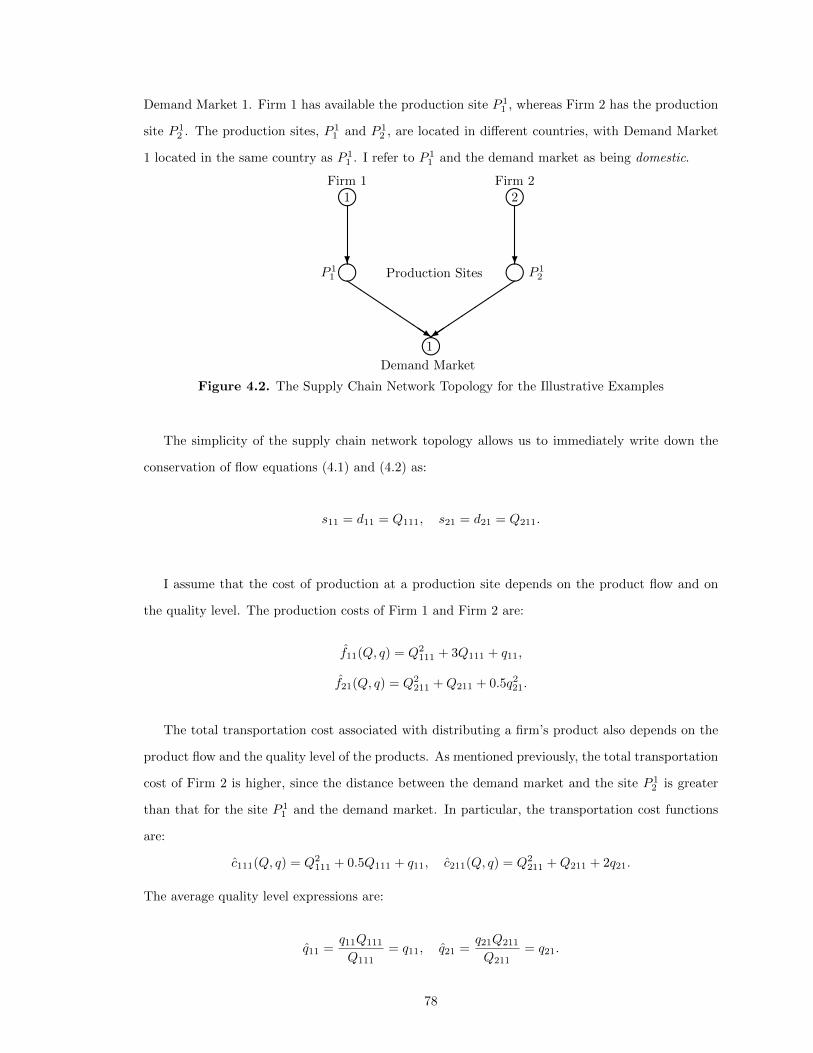
Demand Market 1. Firm 1 has available the production site P 11 , whereas Firm 2 has the production
site P 12 . The production sites, P 1
1 and P 12 , are located in different countries, with Demand Market
1 located in the same country as P 11 . I refer to P 1
1 and the demand market as being domestic.
l1Demand Market
P 11l P 1
2Production Sites l? ?
l1 l2Firm 1 Firm 2
QQQQQQQs
��
���
��+
Figure 4.2. The Supply Chain Network Topology for the Illustrative Examples
The simplicity of the supply chain network topology allows us to immediately write down the
conservation of flow equations (4.1) and (4.2) as:
s11 = d11 = Q111, s21 = d21 = Q211.
I assume that the cost of production at a production site depends on the product flow and on
the quality level. The production costs of Firm 1 and Firm 2 are:
f11(Q, q) = Q2111 + 3Q111 + q11,
f21(Q, q) = Q2211 +Q211 + 0.5q221.
The total transportation cost associated with distributing a firm’s product also depends on the
product flow and the quality level of the products. As mentioned previously, the total transportation
cost of Firm 2 is higher, since the distance between the demand market and the site P 12 is greater
than that for the site P 11 and the demand market. In particular, the transportation cost functions
are:
c111(Q, q) = Q2111 + 0.5Q111 + q11, c211(Q, q) = Q2
211 +Q211 + 2q21.
The average quality level expressions are:
q11 =q11Q111
Q111= q11, q21 =
q21Q211
Q211= q21.
78
The quality upper bounds are: q11 = q21 = 100. The minimum quality standards are: q11
=
q21
= 0.8.
The demand price functions for the products of Firm 1 and Firm 2 at the demand market, are,
in turn, functions of the average quality levels, q11, q22, and the product flows, as follows:
ρ11(Q, q) = −(Q111 +Q211) + 0.5q11 + 20,
ρ21(Q, q) = −(Q211 +Q111) + q21 + 25.
In the following subsections, I first solve variational inequality (4.11) governing the differentiated
supply chain network equilibrium model with quality but without any trade policy instruments.
Then, I incorporate a strict quota, and further demonstrate the equivalence to the model with
a tariff, with the tariff corresponding to the equilibrium Lagrange multiplier associated with the
solution of the former model.
The parameters in the cost and demand functions are reasonable for the size and the location of
the hypothetical firms.
4.1.6.1 Illustrative Example without Trade Interventions
In this example, a strict quota or tariff is not considered, and I solve variational inequality
(4.11). According to (4.11), it is reasonable to make the assumption that Q∗111 > 0, Q∗211 > 0,
q11 > q∗11 > q11
, and q21 > q∗21 > q21
. Therefore, the following expressions are written, all of which
are equal to 0:
∂f11(Q∗, q∗)
∂Q111+∂c111(Q∗, q∗)
∂Q111− ρ11(Q∗, q∗)− ∂ρ11(Q∗, q∗)
∂Q111Q∗111 = 0, (4.25)
∂f11(Q∗, q∗)
∂q11+∂c111(Q∗, q∗)
∂q11− ∂ρ11(Q∗, q)
∂q11Q∗111 = 0, (4.26)
∂f21(Q∗, q∗)
∂Q211+∂c211(Q∗, q∗)
∂Q211− ρ21(Q∗, q∗)− ∂ρ21(Q∗, q∗)
∂Q211Q∗211 = 0, (4.27)
∂f21(Q∗, q∗)
∂q21+∂c211(Q∗, q∗)
∂q21− ∂ρ21(Q∗, q∗)
∂q21Q∗211 = 0. (4.28)
Inserting the corresponding functions into the above equations (4.25) – (4.28), the following
system of equations are obtained:
6Q∗111 +Q∗211 − 0.5q∗11 = 16.5,
79
0.5Q∗111 = 2,
6Q∗211 +Q∗111 − q∗21 = 23,
Q∗211 − q∗21 = 2,
with solution:
Q∗111 = 4.00, Q∗211 = 3.40, q∗11 = q11 = 21.80, q∗21 = q21 = 1.40.
Furthermore, the demand prices at equilibrium, in dollars, are: ρ11 = 23.50 and ρ21 = 19.00.
The profits of the firms, in dollars, are: U1 = 4.40 and U2 = 30.90. It is evident that, even though
the quality of Firm 2 is lower and it sells less at the demand market, it enjoys a higher profit than
Firm 1. This is caused by the fact that the price of Firm 2’s product is lower. The consumer welfare
associated with the two firms’ products is, respectively, CW11 = 8.00 and CW21 = 5.78.
4.1.6.2 An Illustrative Example with a Strict Quota and Tariff Equivalence
I now use, as a baseline, the illustrative example in Subsection 4.1.6.1, and impose a strict
quota on the product flow from the nondomestic production site. Subsequently, I demonstrate the
theoretical result of Section 4.1.4 of the equivalence of the equilibrium solutions to the model with a
strict quota and the model with a tariff, over the same group, through this example, with the tariff
for the latter being set to the equilibrium Lagrange multiplier of the former. The group consists of
the production site P 12 of Firm 2 and Demand Market 1, since the country that the demand market
is located in imposes a quota on the products from the country that the production site P 12 of Firm
2 is located in. Hence, the strict quota Q is imposed only on the product flow in this group. The
strict quota Q = 3 is set and, consequently, the strict quota constraint in (4.12) becomes:
Q211 ≤ 3, (4.29)
Similar to the expressions in (4.25) – (4.28), the variational inequality formulation in (4.16) yields
the following expressions, which are all equal 0, since it is reasonable that the equilibrium product
flows will be positive and the quality levels will not be at the boundaries:
∂f11(Q∗, q∗)
∂Q111+∂c111(Q∗, q∗)
∂Q111− ρ11(Q∗, q∗)− ∂ρ11(Q∗, q∗)
∂Q111Q∗111 = 0, (4.30)
80
∂f11(Q∗, q∗)
∂q11+∂c111(Q∗, q∗)
∂q11− ∂ρ11(Q∗, q∗)
∂q11Q∗111 = 0, (4.31)
∂f21(Q∗, q∗)
∂Q211+∂c211(Q∗, q∗)
∂Q211− ρ21(Q∗, q∗)− ∂ρ21(Q∗, q∗)
∂Q211Q∗211 + λ∗ = 0, (4.32)
∂f21(Q∗, q∗)
∂q21+∂c211(Q∗, q∗)
∂q21− ∂ρ21(Q∗, q∗)
∂q21Q∗211 = 0, (4.33)
Q−Q∗211 = 0. (4.34)
Notice that the expressions are very similar to (4.25) - (4.28). However, now, in (4.32), the
Lagrange multiplier associated with the strict quota constraint (4.29) is added and (4.34) is a new
linear equation.
By inserting the appropriate functions into (4.30) – (4.33), with the strict quota Q = 3, the
following system of equations are obtained:
6Q∗111 +Q∗211 − 0.5q∗11 = 16.5,
0.5Q∗111 = 2,
6Q∗211 +Q∗111 − q∗21 + λ∗ = 23,
Q∗211 − q∗21 = 2,
Q∗211 = 3.
The equilibrium product flows, quality levels, and the Lagrange multiplier are, hence:
Q∗111 = 4.00, Q∗211 = 3.00, q∗11 = q11 = 21.00, q∗21 = q21 = 1.00,
λ∗ = 2.00.
The demand prices at equilibrium of Firm 1 and Firm 2 are: ρ11 = 23.50 and ρ21 = 19.00 and are
the same as in the example without the strict quota. The profits of the firms are now: U1 = 6.00 and
U2 = 24.50. With the strict quota imposed, the quality levels of the products, as well as the average
quality at the demand market, decrease from their respective values when there is no imposed quota.
In addition, the consumer welfare associated with the firms’ products are now: CW11 = 8.00 and
CW21 = 4.50. The value of CW21 is lower than the corresponding one for the example without a
strict quota.
Further, by using the result obtained in Section 4.1.4 on the equivalence of the equilibrium
solution to the model with a strict quota and that of the model with a tariff (over the same group),
81
provided that the equilibrium Lagrange multiplier obtained in the solution of the model with a strict
quota is the assigned tariff for the group in the tariff model, the equilibrium tariff τ∗ = λ∗ = 2.00
satisfies the variational inequality formulation (4.18). Clearly, the above equilibrium product flows
and equilibrium quality levels then solve VI (4.18).
Hence, the above numerical example demonstrates that a strict quota or tariff may adversely
affect both the quality of the products and the consumer welfare, which is clearly not good for
consumers. However, the profit of the domestic firm increases, whereas that of the firm with the
nondomestic production site decreases.
4.2. The Algorithm
The explicit formulae of the modified projection method (cf. Section 2.4.2) for the solution of
variational inequality variational inequality (4.23), equivalently (4.15), are provided below, where t
is the iteration counter.
4.2.1 Explicit Formulae for the Differentiated Product Supply Chain Network Equi-
librium Model Variables without Trade Interventions in Step 1 of the Modified
Projection Method
Qt+1ijk = max{0, Qtijk + β(ρik(Qt, qt) +
nD∑l=1
∂ρil(Qt, qt)
∂Qijk
ni∑h=1
Qtihl −ni∑h=1
∂fih(Qt, qt)
∂Qijk
−ni∑h=1
nD∑l=1
∂cihl(Qt, qt)
∂Qijk)}, i = 1, . . . , I; j = 1, . . . , ni; k = 1, . . . , nD, (4.35)
qt+1ij = max{ qij ,min{qij , qtij + β(
nD∑k=1
∂ρik(Qt, qt)
∂qij
ni∑h=1
Qtihk −ni∑h=1
∂fih(Qt, qt)
∂qij
−ni∑h=1
nD∑k=1
∂cihk(Qt, qt)
∂qij)}}, i = 1, . . . , I; j = 1, . . . , ni. (4.36)
4.2.2 Explicit Formulae for the Differentiated Product Supply Chain Network Equi-
librium Model Variables with a Strict Quota in Step 1 of the Modified Projection
Method
Qt+1ijk = max{0, Qtijk + β(ρik(Qt, qt) +
nD∑l=1
∂ρil(Qt, qt)
∂Qijk
ni∑h=1
Qtihl −ni∑h=1
∂fih(Qt, qt)
∂Qijk
82
−ni∑h=1
nD∑l=1
∂cihl(Qt, qt)
∂Qijk− λt)}, i = 1, . . . , I; j = 1, . . . , ni; k = 1, . . . , nD; (j, k) ∈ G, (4.37)
λt+1 = max{0, λt + β(
I∑i=1
∑(j,k)∈G
Qtijk − Q)}. (4.38)
The explicit formulae for the product shipments, Qt+1ijk ; i = 1, . . . , I; j = 1, . . . , ni; k = 1, . . . , nD;
(j, k) 6∈ G, are the same as in (4.37), with the explicit formulae for product quality, qt+1ij ; i =
1, . . . , I; j = 1, . . . , ni, the same as in (4.38).
4.2.3 Explicit Formulae for the Differentiated Product Supply Chain Network Equi-
librium Model Variables with a Tariff in Step 1 of the Modified Projection
Method
Qt+1ijk = max{0, Qtijk + β(ρik(Qt, qt) +
nD∑l=1
∂ρil(Qt, qt)
∂Qijk
ni∑h=1
Qtihl −ni∑h=1
∂fih(Qt, qt)
∂Qijk
−ni∑h=1
nD∑l=1
∂cihl(Qt, qt)
∂Qijk− τ∗)}, i = 1, . . . , I; j = 1, . . . , ni; k = 1, . . . , nD; (j, k) ∈ G. (4.39)
The explicit formulae for the product shipments, Qt+1ijk ; i = 1, . . . , I; j = 1, . . . , ni; k = 1, . . . , nD;
(j, k) 6∈ G, and for product quality, qt+1ij ; i = 1, . . . , I; j = 1, . . . , ni, are the same as in (4.35) and
(4.36), respectively.
4.3. Numerical Examples
In this section, I focus on the supply chain network of soybeans, an agricultural product that has
a great impact on today’s agricultural trade. Soybeans were discovered and domesticated in China
over 3000 years ago, with the United States being a leader in producing, consuming, and exporting
soybeans globally (Song, Xu, and Marchant (2004)). In the United States, soybean production and
export have become essential parts of the agricultural economy, with soybeans ranked second among
crops in farm value in 2005 (Ash, Livesey, and Dohlman (2006)). Lundgren (2018) reports that, in
2018, soybean production in the United States reached 5.11 billion bushels with an export of 2.13
billion bushels.
China, in turn, is the largest importer of soybeans due to its rapidly increasing population size
(Brown (2012)). The consumption of soybeans in China, in 2017, was reported to be 112.18 million
tons, but the domestic production volume was only 13 million tons (Wood (2018)). Due to this
83
huge gap, China has to rely heavily on soybeans imported from foreign countries, such as the United
States, Brazil, and Argentina.
In 2018, the trade war between China and the United States escalated, with the Chinese gov-
ernment imposing quotas and tariffs on the soybeans exported from the United States in retaliation
(Wong and Koty (2019)). According to Appelbaum (2018), this created an opportunity for other
large soybean exporters, such as Brazil and Argentina. In 2017, Brazil exported 53.8 million tons
of soybeans to China, corresponding to 75% of its production volume (Zhou et al. (2018)). Shane
(2018) claims that, the Chinese importer, Hebei Power Sea Feed Technology, bought thousands of
tons of soybeans for animal feed from Brazil instead of the United States in 2018.
In this section, I present a series of numerical examples comprising a case study for the differ-
entiated product supply chain network equilibrium models for soybeans, and examine the effects
of quotas and tariffs on soybean trade and quality. The models in the case study were solved via
the the modified projection method, which was implemented in Matlab on an OS X 10.14.1 system.
The convergence tolerance was: 10−6, so that the algorithm was deemed to have converged when
the absolute value of the difference between each successive product shipment, quality level, and the
Lagrange multiplier was less than or equal to 10−6. I set β in the algorithm to .15 and initialized
the algorithm with the product shipments equal to 100 and with the quality levels and the Lagrange
multiplier equal to 0.
The baseline example, Example 4.1, has no quotas or tariffs imposed. In subsequent examples,
I add strict quotas, tariffs, and then also consider the addition of a demand market.
4.3.1 Example 4.1: 2 Firms, with 3 Production Sites for the First Firm, Two Produc-
tion Sites for the Second, and a Single Demand Market
The supply chain network for soybeans for Example 4.1 is depicted in Figure 4.3. There are two
producing firms, Firm 1 and Firm 2, which are located in the United States. The firms are assumed to
be Cargill and Archer Daniels Midland Company (ADM), two of the largest agricultural companies
in the United States with production sites in the United States and overseas (Zhou et al. (2018)).
Recall that the middle nodes represent production sites. Cargill owns three production sites, P 11 ,
P 12 , and P 1
3 , which are located in the United States, Brazil, and Argentina, respectively. ADM’s
production sites are denoted by P 21 and P 2
2 , and they are located, respectively, in the United States
84
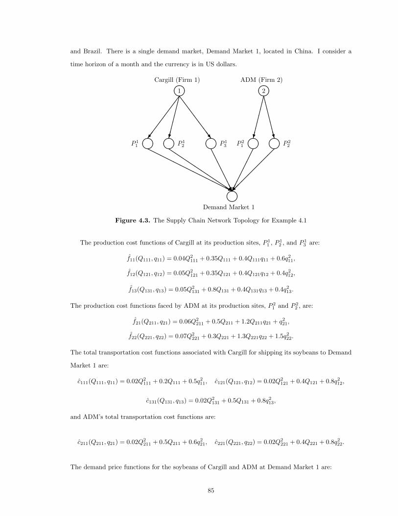
and Brazil. There is a single demand market, Demand Market 1, located in China. I consider a
time horizon of a month and the currency is in US dollars.
� ��1��������
�������/
SSSSSSSw
Cargill (Firm 1) ADM (Firm 2)
� ��2��������
CCCCCCCW� ��� �� � �� � ��� ��P 1
1 P 12 P 1
3 P 21 P 2
2
� ��
HHHHHH
HHHHHH
HHj
QQQQQQQQQQs
AAAAAAAU
��������
��
��
���
Demand Market 1
Figure 4.3. The Supply Chain Network Topology for Example 4.1
The production cost functions of Cargill at its production sites, P 11 , P 1
2 , and P 13 are:
f11(Q111, q11) = 0.04Q2111 + 0.35Q111 + 0.4Q111q11 + 0.6q211,
f12(Q121, q12) = 0.05Q2121 + 0.35Q121 + 0.4Q121q12 + 0.4q212,
f13(Q131, q13) = 0.05Q2131 + 0.8Q131 + 0.4Q131q13 + 0.4q213.
The production cost functions faced by ADM at its production sites, P 21 and P 2
2 , are:
f21(Q211, q21) = 0.06Q2211 + 0.5Q211 + 1.2Q211q21 + q221,
f22(Q221, q22) = 0.07Q2221 + 0.3Q221 + 1.3Q221q22 + 1.5q222.
The total transportation cost functions associated with Cargill for shipping its soybeans to Demand
Market 1 are:
c111(Q111, q11) = 0.02Q2111 + 0.2Q111 + 0.5q211, c121(Q121, q12) = 0.02Q2
121 + 0.4Q121 + 0.8q212,
c131(Q131, q13) = 0.02Q2131 + 0.5Q131 + 0.8q213,
and ADM’s total transportation cost functions are:
c211(Q211, q21) = 0.02Q2211 + 0.5Q211 + 0.6q221, c221(Q221, q22) = 0.02Q2
221 + 0.4Q221 + 0.8q222.
The demand price functions for the soybeans of Cargill and ADM at Demand Market 1 are:
85
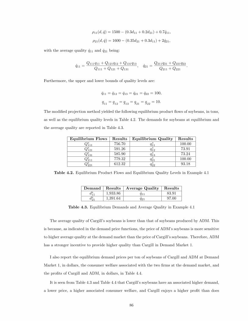
ρ11(d, q) = 1500− (0.3d11 + 0.2d21) + 0.7q11,
ρ21(d, q) = 1600− (0.35d21 + 0.3d11) + 2q21,
with the average quality q11 and q21 being:
q11 =Q111q11 +Q121q12 +Q131q13
Q111 +Q121 +Q131, q21 =
Q211q21 +Q221q22Q211 +Q221
.
Furthermore, the upper and lower bounds of quality levels are:
q11 = q12 = q13 = q21 = q22 = 100,
q11
= q12
= q13
= q21
= q22
= 10.
The modified projection method yielded the following equilibrium product flows of soybeans, in tons,
as well as the equilibrium quality levels in Table 4.2. The demands for soybeans at equilibrium and
the average quality are reported in Table 4.3.
Equilibrium Flows Results Equilibrium Quality ResultsQ∗111 756.70 q∗11 100.00Q∗121 591.26 q∗12 73.91Q∗131 585.90 q∗13 73.24Q∗211 779.32 q∗21 100.00Q∗221 612.32 q∗22 93.18
Table 4.2. Equilibrium Product Flows and Equilibrium Quality Levels in Example 4.1
Demand Results Average Quality Resultsd∗11 1,933.86 q11 83.91d∗21 1,391.64 q21 97.00
Table 4.3. Equilibrium Demands and Average Quality in Example 4.1
The average quality of Cargill’s soybeans is lower than that of soybeans produced by ADM. This
is because, as indicated in the demand price functions, the price of ADM’s soybeans is more sensitive
to higher average quality at the demand market than the price of Cargill’s soybeans. Therefore, ADM
has a stronger incentive to provide higher quality than Cargill in Demand Market 1.
I also report the equilibrium demand prices per ton of soybeans of Cargill and ADM at Demand
Market 1, in dollars, the consumer welfare associated with the two firms at the demand market, and
the profits of Cargill and ADM, in dollars, in Table 4.4.
It is seen from Table 4.3 and Table 4.4 that Cargill’s soybeans have an associated higher demand,
a lower price, a higher associated consumer welfare, and Cargill enjoys a higher profit than does
86
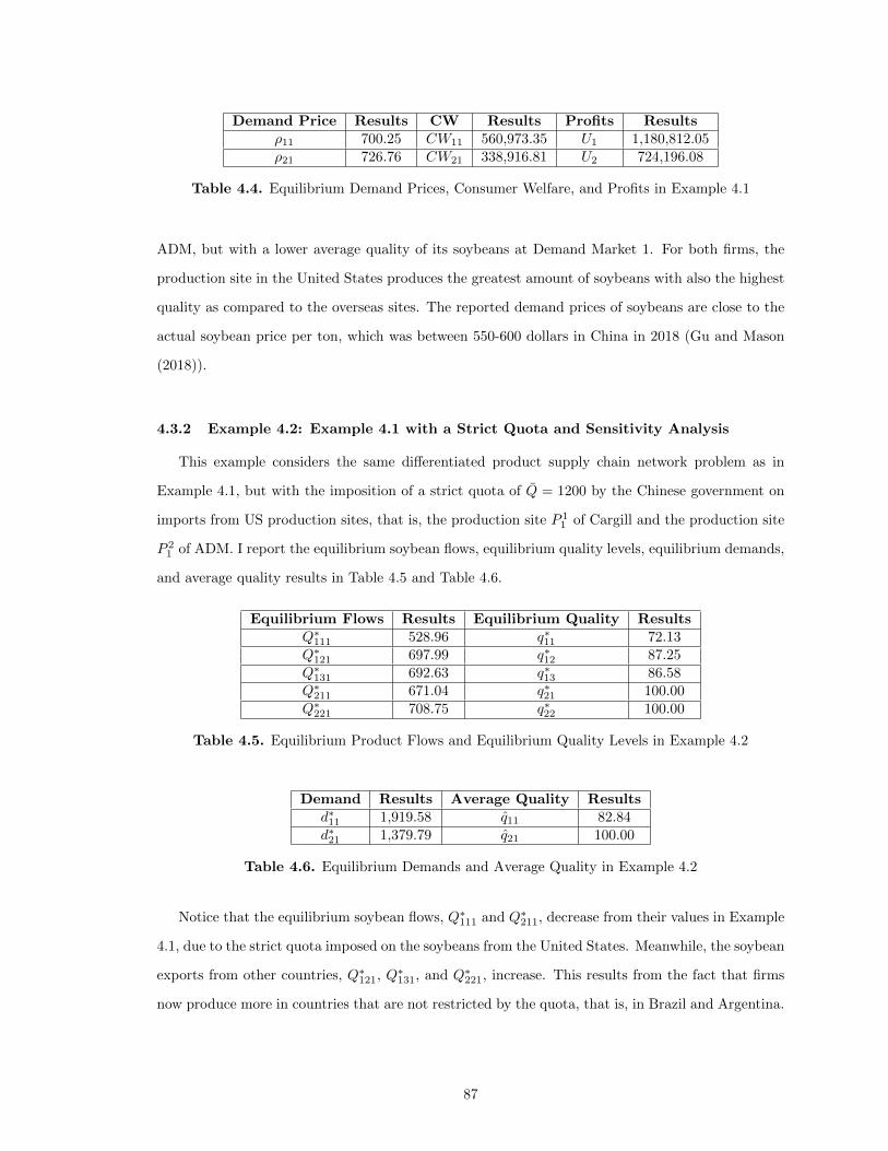
Demand Price Results CW Results Profits Resultsρ11 700.25 CW11 560,973.35 U1 1,180,812.05ρ21 726.76 CW21 338,916.81 U2 724,196.08
Table 4.4. Equilibrium Demand Prices, Consumer Welfare, and Profits in Example 4.1
ADM, but with a lower average quality of its soybeans at Demand Market 1. For both firms, the
production site in the United States produces the greatest amount of soybeans with also the highest
quality as compared to the overseas sites. The reported demand prices of soybeans are close to the
actual soybean price per ton, which was between 550-600 dollars in China in 2018 (Gu and Mason
(2018)).
4.3.2 Example 4.2: Example 4.1 with a Strict Quota and Sensitivity Analysis
This example considers the same differentiated product supply chain network problem as in
Example 4.1, but with the imposition of a strict quota of Q = 1200 by the Chinese government on
imports from US production sites, that is, the production site P 11 of Cargill and the production site
P 21 of ADM. I report the equilibrium soybean flows, equilibrium quality levels, equilibrium demands,
and average quality results in Table 4.5 and Table 4.6.
Equilibrium Flows Results Equilibrium Quality ResultsQ∗111 528.96 q∗11 72.13Q∗121 697.99 q∗12 87.25Q∗131 692.63 q∗13 86.58Q∗211 671.04 q∗21 100.00Q∗221 708.75 q∗22 100.00
Table 4.5. Equilibrium Product Flows and Equilibrium Quality Levels in Example 4.2
Demand Results Average Quality Resultsd∗11 1,919.58 q11 82.84d∗21 1,379.79 q21 100.00
Table 4.6. Equilibrium Demands and Average Quality in Example 4.2
Notice that the equilibrium soybean flows, Q∗111 and Q∗211, decrease from their values in Example
4.1, due to the strict quota imposed on the soybeans from the United States. Meanwhile, the soybean
exports from other countries, Q∗121, Q∗131, and Q∗221, increase. This results from the fact that firms
now produce more in countries that are not restricted by the quota, that is, in Brazil and Argentina.
87
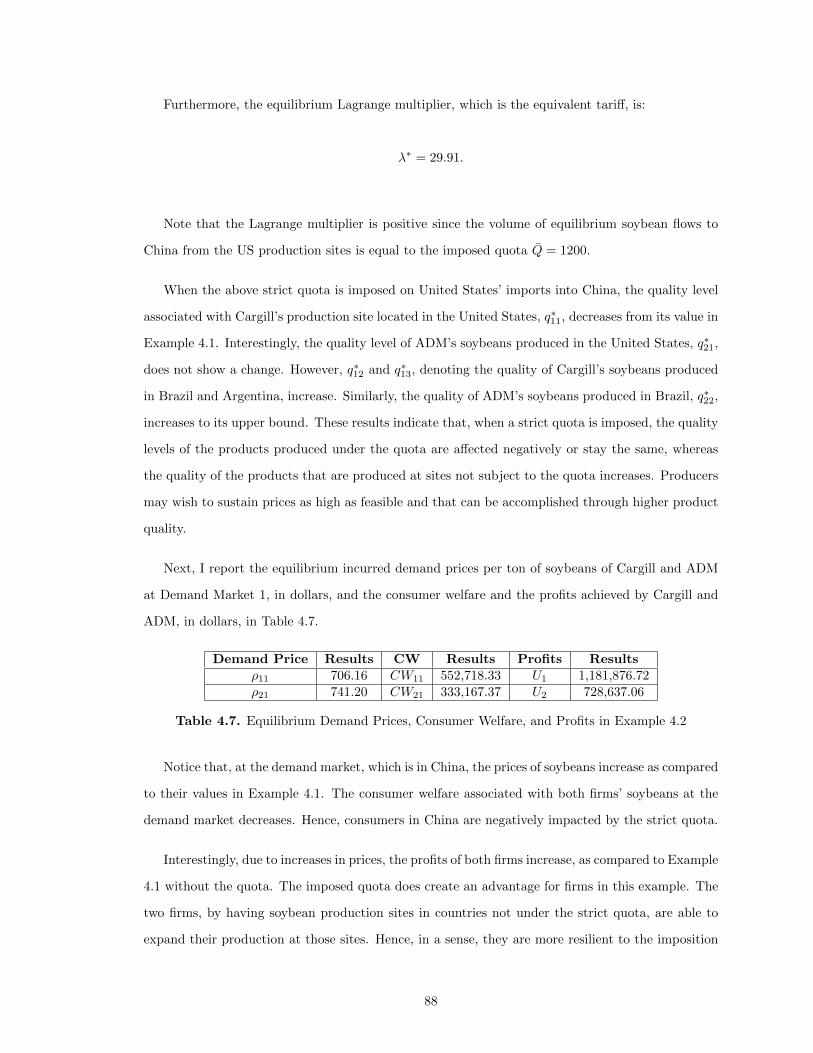
Furthermore, the equilibrium Lagrange multiplier, which is the equivalent tariff, is:
λ∗ = 29.91.
Note that the Lagrange multiplier is positive since the volume of equilibrium soybean flows to
China from the US production sites is equal to the imposed quota Q = 1200.
When the above strict quota is imposed on United States’ imports into China, the quality level
associated with Cargill’s production site located in the United States, q∗11, decreases from its value in
Example 4.1. Interestingly, the quality level of ADM’s soybeans produced in the United States, q∗21,
does not show a change. However, q∗12 and q∗13, denoting the quality of Cargill’s soybeans produced
in Brazil and Argentina, increase. Similarly, the quality of ADM’s soybeans produced in Brazil, q∗22,
increases to its upper bound. These results indicate that, when a strict quota is imposed, the quality
levels of the products produced under the quota are affected negatively or stay the same, whereas
the quality of the products that are produced at sites not subject to the quota increases. Producers
may wish to sustain prices as high as feasible and that can be accomplished through higher product
quality.
Next, I report the equilibrium incurred demand prices per ton of soybeans of Cargill and ADM
at Demand Market 1, in dollars, and the consumer welfare and the profits achieved by Cargill and
ADM, in dollars, in Table 4.7.
Demand Price Results CW Results Profits Resultsρ11 706.16 CW11 552,718.33 U1 1,181,876.72ρ21 741.20 CW21 333,167.37 U2 728,637.06
Table 4.7. Equilibrium Demand Prices, Consumer Welfare, and Profits in Example 4.2
Notice that, at the demand market, which is in China, the prices of soybeans increase as compared
to their values in Example 4.1. The consumer welfare associated with both firms’ soybeans at the
demand market decreases. Hence, consumers in China are negatively impacted by the strict quota.
Interestingly, due to increases in prices, the profits of both firms increase, as compared to Example
4.1 without the quota. The imposed quota does create an advantage for firms in this example. The
two firms, by having soybean production sites in countries not under the strict quota, are able to
expand their production at those sites. Hence, in a sense, they are more resilient to the imposition
88
of a quota than they might be otherwise. In a later example, Example 4.4, I consider the same
problem as in Example 4.2 but with Cargill’s production site in the United States shut down.
4.3.3 Sensitivity Analysis: Impacts of a Quality Coefficient Change in a Cost Functions
I now test the robustness of the managerial insights achieved in Example 4.2. Specifically, I
test whether the following four insights obtained from the solution of Example 4.2 also hold when
varying the quality coefficient in a production cost function, f12, not under a strict quota.
Recall that, in Example 4.2, with the imposition of a strict quota, Q = 1200, by China on imports
from the United States, the following results were observed:
1. The soybean flows from the United States production sites, Q∗111 and Q∗211, decreased. Meanwhile,
the soybean exports from other countries, Q∗121, Q∗131, and Q∗221, increased.
2. The quality levels of the soybeans produced in the United States, q∗11 and q∗21, decreased or stayed
the same. However, q∗12, q∗13, and q∗22, denoting the quality of the soybeans produced elsewhere,
increased.
3. At the demand market, the prices of soybeans increased.
4. The consumer welfare associated with both firms’ soybeans decreased, but both firms made higher
profits.
In Tables 4.8 and 4.9 I provide sensitivity analysis results for Example 4.2 by varying the coeffi-
cient of q212 in f12, with and without the strict quota. The values of the coefficient are: 0.2, 0.4, 0.6,
0.8, and 1, respectively. “Coeff.” in Tables 4.8 and 4.9 denotes “Coefficient.”
As can be observed from Tables 4.8 and 4.9, points 1, 2, 3, and 4 above hold even with a varying
quality coefficient in f12. The generality of the model and computational procedure allows for such
flexibility. Of course, sensitivity analyses can be conducted by varying other coefficients in the other
production cost functions, as well as in the transportation cost functions, both individually and
jointly.
4.3.4 Sensitivity Analysis: Impacts of Changes in the Strict Quota
I now provide a sensitivity analysis examining the effects of the value of the strict quota on the
equilibrium product flows, the quality levels, and the average quality levels, demands, demand prices,
89
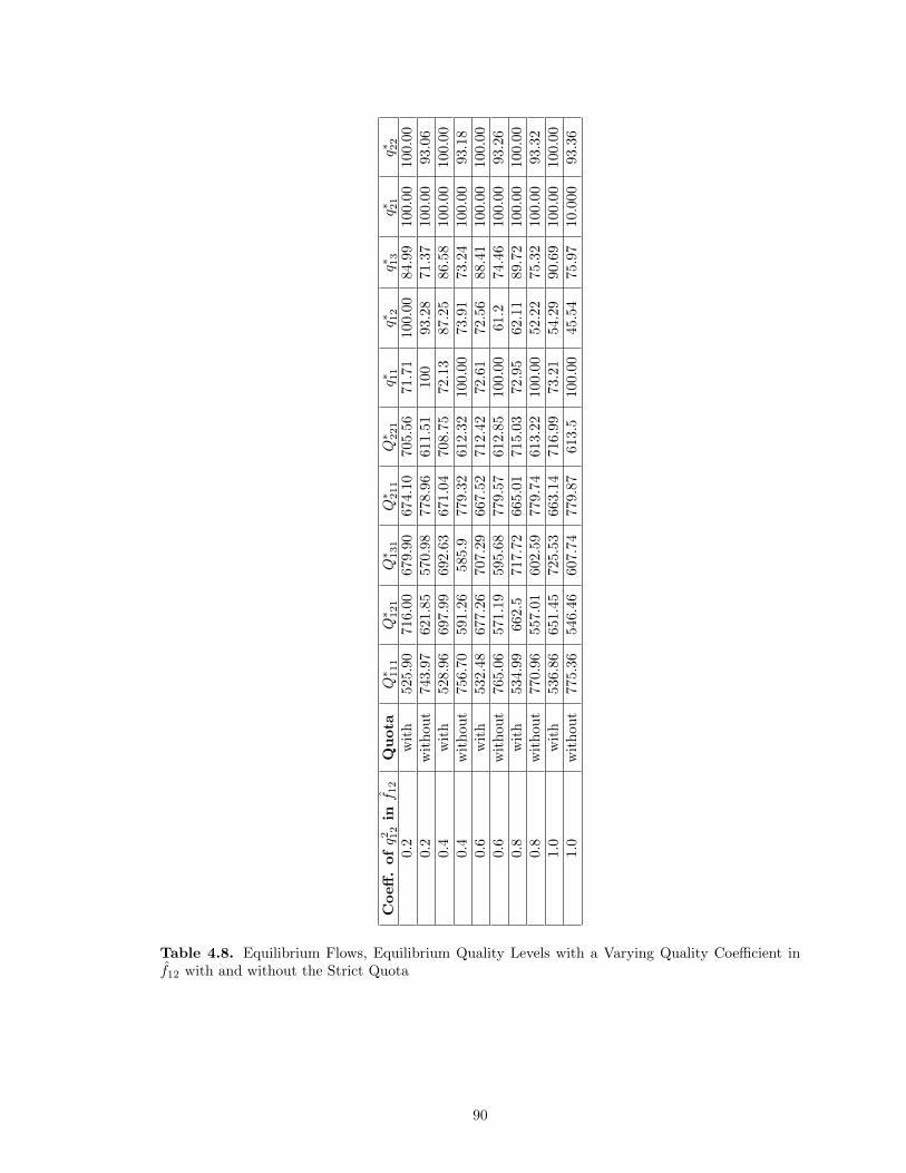
Coeff
.ofq2 1
2in
f 12
Qu
ota
Q∗ 11
1Q∗ 12
1Q∗ 13
1Q∗ 21
1Q∗ 22
1q∗ 1
1q∗ 1
2q∗ 1
3q∗ 2
1q∗ 2
2
0.2
wit
h52
5.90
716.0
0679.9
0674.1
0705.5
671.7
1100.0
084.9
9100.0
0100.0
00.
2w
ith
out
743.
97621.8
5570.9
8778.9
6611.5
1100
93.2
871.3
7100.0
093.0
60.
4w
ith
528.
96697.9
9692.6
3671.0
4708.7
572.1
387.2
586.5
8100.0
0100.0
00.
4w
ith
out
756.
70591.2
6585.9
779.3
2612.3
2100.0
073.9
173.2
4100.0
093.1
80.
6w
ith
532.
48677.2
6707.2
9667.5
2712.4
272.6
172.5
688.4
1100.0
0100.0
00.
6w
ith
out
765.
06571.1
9595.6
8779.5
7612.8
5100.0
061.2
74.4
6100.0
093.2
60.
8w
ith
534.
99662.5
717.7
2665.0
1715.0
372.9
562.1
189.7
2100.0
0100.0
00.
8w
ith
out
770.
96557.0
1602.5
9779.7
4613.2
2100.0
052.2
275.3
2100.0
093.3
21.
0w
ith
536.
86651.4
5725.5
3663.1
4716.9
973.2
154.2
990.6
9100.0
0100.0
01.
0w
ith
out
775.
36546.4
6607.7
4779.8
7613.5
100.0
045.5
475.9
710.0
00
93.3
6
Table 4.8. Equilibrium Flows, Equilibrium Quality Levels with a Varying Quality Coefficient inf12 with and without the Strict Quota
90
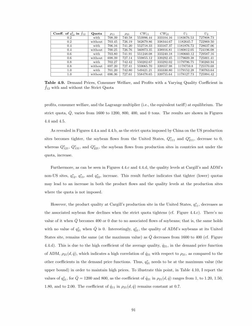
Coeff. of q212 in f12 Quota ρ11 ρ21 CW11 CW21 U1 U2
0.2 with 708.39 740.58 553996.44 333104.16 1183676.53 727808.730.2 without 703.45 726.19 562679.86 338344.67 1182645.7 722969.500.4 with 706.16 741.20 552718.33 333167.37 1181876.72 728637.060.4 without 700.25 726.76 560973.35 338916.81 1180812.05 724196.080.6 with 703.80 741.91 551248.08 333240.18 1180660.12 729587.160.6 without 698.39 727.14 559855.12 339292.45 1179609.38 725001.410.8 with 702.27 742.42 550202.67 333292.02 1179796.75 730260.940.8 without 697.20 727.41 559065.70 339557.98 1178759.8 725570.681.0 with 701.20 742.80 549421.21 333330.80 1179152.28 730763.641.0 without 696.36 727.61 558478.65 339755.64 1178127.73 725994.42
Table 4.9. Demand Prices, Consumer Welfare, and Profits with a Varying Quality Coefficient inf12 with and without the Strict Quota
profits, consumer welfare, and the Lagrange multiplier (i.e., the equivalent tariff) at equilibrium. The
strict quota, Q, varies from 1600 to 1200, 800, 400, and 0 tons. The results are shown in Figures
4.4 and 4.5.
As revealed in Figures 4.4.a and 4.4.b, as the strict quota imposed by China on the US production
sites becomes tighter, the soybean flows from the United States, Q∗111 and Q∗211, decrease to 0,
whereas Q∗121, Q∗131, and Q∗221, the soybean flows from production sites in countries not under the
quota, increase.
Furthermore, as can be seen in Figures 4.4.c and 4.4.d, the quality levels at Cargill’s and ADM’s
non-US sites, q∗12, q∗13, and q∗22, increase. This result further indicates that tighter (lower) quotas
may lead to an increase in both the product flows and the quality levels at the production sites
where the quota is not imposed.
However, the product quality at Cargill’s production site in the United States, q∗11, decreases as
the associated soybean flow declines when the strict quota tightens (cf. Figure 4.4.c). There’s no
value of it when Q becomes 400 or 0 due to no associated flows of soybeans; that is, the same holds
with no value of q∗21 when Q is 0. Interestingly, q∗21, the quality of ADM’s soybeans at its United
States site, remains the same (at the maximum value) as Q decreases from 1600 to 400 (cf. Figure
4.4.d). This is due to the high coefficient of the average quality, q21, in the demand price function
of ADM, ρ21(d, q), which indicates a high correlation of q21 with respect to ρ21, as compared to the
other coefficients in the demand price functions. Thus, q∗21 needs to be at the maximum value (the
upper bound) in order to maintain high prices. To illustrate this point, in Table 4.10, I report the
values of q∗21, for Q = 1200 and 800, as the coefficient of q21 in ρ21(d, q) ranges from 1, to 1.20, 1.50,
1.80, and to 2.00. The coefficient of q11 in ρ21(d, q) remains constant at 0.7.
91
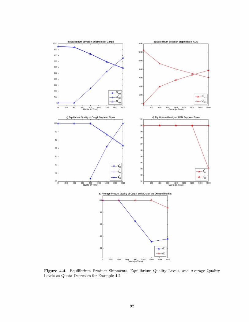
Figure 4.4. Equilibrium Product Shipments, Equilibrium Quality Levels, and Average QualityLevels as Quota Decreases for Example 4.2
92
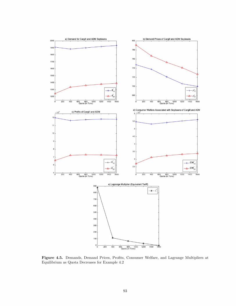
Figure 4.5. Demands, Demand Prices, Profits, Consumer Welfare, and Lagrange Multipliers atEquilibrium as Quota Decreases for Example 4.2
93
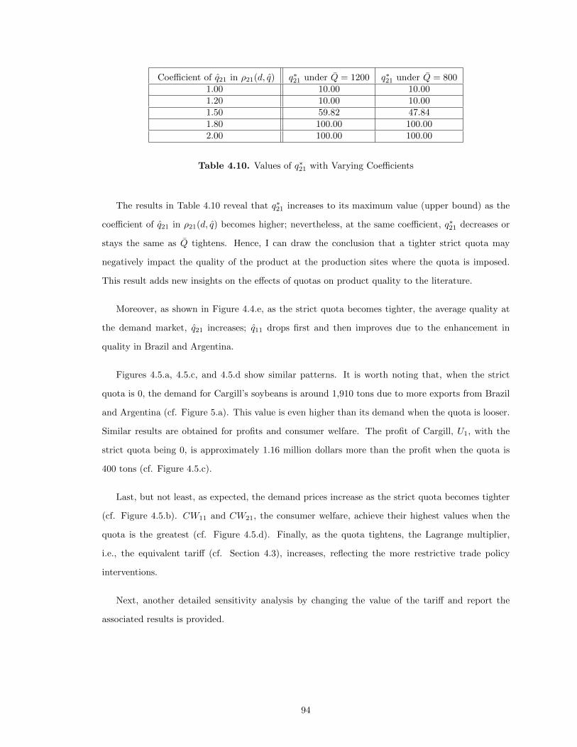
Coefficient of q21 in ρ21(d, q) q∗21 under Q = 1200 q∗21 under Q = 8001.00 10.00 10.001.20 10.00 10.001.50 59.82 47.841.80 100.00 100.002.00 100.00 100.00
Table 4.10. Values of q∗21 with Varying Coefficients
The results in Table 4.10 reveal that q∗21 increases to its maximum value (upper bound) as the
coefficient of q21 in ρ21(d, q) becomes higher; nevertheless, at the same coefficient, q∗21 decreases or
stays the same as Q tightens. Hence, I can draw the conclusion that a tighter strict quota may
negatively impact the quality of the product at the production sites where the quota is imposed.
This result adds new insights on the effects of quotas on product quality to the literature.
Moreover, as shown in Figure 4.4.e, as the strict quota becomes tighter, the average quality at
the demand market, q21 increases; q11 drops first and then improves due to the enhancement in
quality in Brazil and Argentina.
Figures 4.5.a, 4.5.c, and 4.5.d show similar patterns. It is worth noting that, when the strict
quota is 0, the demand for Cargill’s soybeans is around 1,910 tons due to more exports from Brazil
and Argentina (cf. Figure 5.a). This value is even higher than its demand when the quota is looser.
Similar results are obtained for profits and consumer welfare. The profit of Cargill, U1, with the
strict quota being 0, is approximately 1.16 million dollars more than the profit when the quota is
400 tons (cf. Figure 4.5.c).
Last, but not least, as expected, the demand prices increase as the strict quota becomes tighter
(cf. Figure 4.5.b). CW11 and CW21, the consumer welfare, achieve their highest values when the
quota is the greatest (cf. Figure 4.5.d). Finally, as the quota tightens, the Lagrange multiplier,
i.e., the equivalent tariff (cf. Section 4.3), increases, reflecting the more restrictive trade policy
interventions.
Next, another detailed sensitivity analysis by changing the value of the tariff and report the
associated results is provided.
94
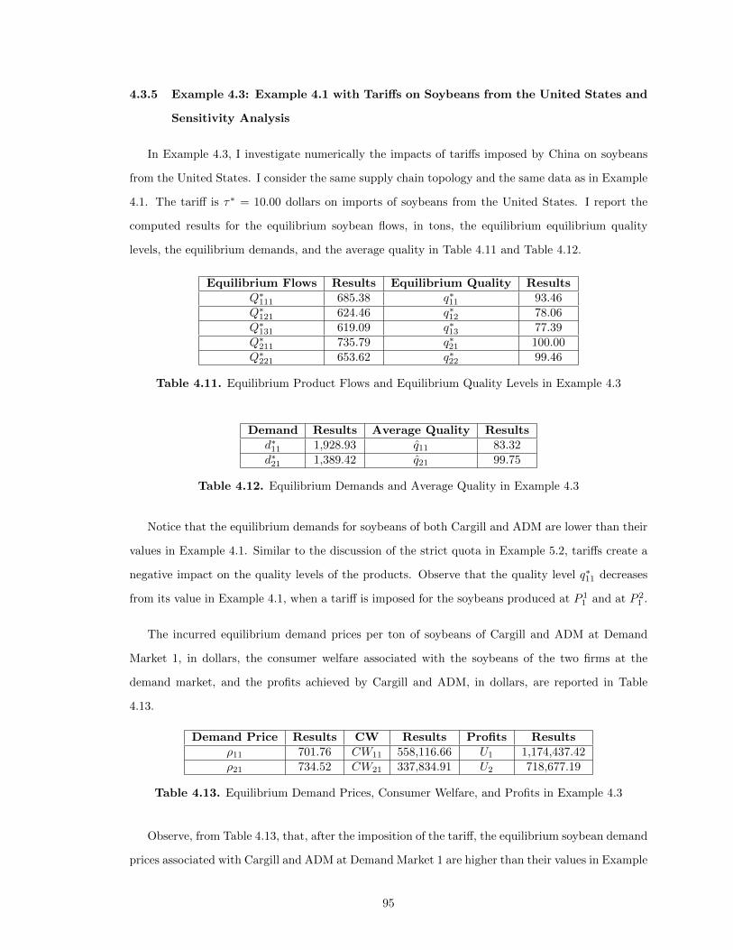
4.3.5 Example 4.3: Example 4.1 with Tariffs on Soybeans from the United States and
Sensitivity Analysis
In Example 4.3, I investigate numerically the impacts of tariffs imposed by China on soybeans
from the United States. I consider the same supply chain topology and the same data as in Example
4.1. The tariff is τ∗ = 10.00 dollars on imports of soybeans from the United States. I report the
computed results for the equilibrium soybean flows, in tons, the equilibrium equilibrium quality
levels, the equilibrium demands, and the average quality in Table 4.11 and Table 4.12.
Equilibrium Flows Results Equilibrium Quality ResultsQ∗111 685.38 q∗11 93.46Q∗121 624.46 q∗12 78.06Q∗131 619.09 q∗13 77.39Q∗211 735.79 q∗21 100.00Q∗221 653.62 q∗22 99.46
Table 4.11. Equilibrium Product Flows and Equilibrium Quality Levels in Example 4.3
Demand Results Average Quality Resultsd∗11 1,928.93 q11 83.32d∗21 1,389.42 q21 99.75
Table 4.12. Equilibrium Demands and Average Quality in Example 4.3
Notice that the equilibrium demands for soybeans of both Cargill and ADM are lower than their
values in Example 4.1. Similar to the discussion of the strict quota in Example 5.2, tariffs create a
negative impact on the quality levels of the products. Observe that the quality level q∗11 decreases
from its value in Example 4.1, when a tariff is imposed for the soybeans produced at P 11 and at P 2
1 .
The incurred equilibrium demand prices per ton of soybeans of Cargill and ADM at Demand
Market 1, in dollars, the consumer welfare associated with the soybeans of the two firms at the
demand market, and the profits achieved by Cargill and ADM, in dollars, are reported in Table
4.13.
Demand Price Results CW Results Profits Resultsρ11 701.76 CW11 558,116.66 U1 1,174,437.42ρ21 734.52 CW21 337,834.91 U2 718,677.19
Table 4.13. Equilibrium Demand Prices, Consumer Welfare, and Profits in Example 4.3
Observe, from Table 4.13, that, after the imposition of the tariff, the equilibrium soybean demand
prices associated with Cargill and ADM at Demand Market 1 are higher than their values in Example
95
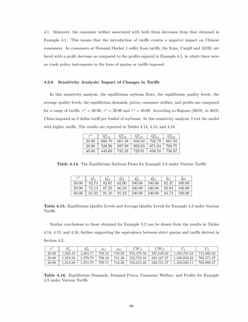
4.1. Moreover, the consumer welfare associated with both firms decreases from that obtained in
Example 4.1. This means that the introduction of tariffs creates a negative impact on Chinese
consumers. As consumers at Demand Market 1 suffer from tariffs, the firms, Cargill and ADM, are
faced with a profit decrease as compared to the profits enjoyed in Example 4.1, in which there were
no trade policy instruments in the form of quotas or tariffs imposed.
4.3.6 Sensitivity Analysis: Impact of Changes in Tariffs
In this sensitivity analysis, the equilibrium soybean flows, the equilibrium quality levels, the
average quality levels, the equilibrium demands, prices, consumer welfare, and profits are computed
for a range of tariffs: τ∗ = 20.00, τ∗ = 29.90 and τ∗ = 40.00. According to Rapoza (2019), in 2019,
China imposed an 8 dollar tariff per bushel of soybeans. In this sensitivity analysis, I test the model
with higher tariffs. The results are reported in Tables 4.14, 4.15, and 4.16.
τ∗ Q∗111 Q∗121 Q∗131 Q∗211 Q∗22120.00 606.79 661.38 656.02 702.79 681.9229.90 528.96 697.99 692.63 671.04 708.7540.00 449.69 735.28 729.91 638.70 736.07
Table 4.14. The Equilibrium Soybean Flows for Example 4.3 under Various Tariffs
τ∗ q∗11 q∗12 q∗13 q∗21 q∗22 q11 q2120.00 82.74 82.67 82.00 100.00 100.00 82.47 100.0029.90 72.13 87.25 86.58 100.00 100.00 82.84 100.0040.00 61.32 91.10 91.24 100.00 100.00 84.74 100.00
Table 4.15. Equilibrium Quality Levels and Average Quality Levels for Example 4.3 under VariousTariffs
Similar conclusions to those obtained for Example 5.2 can be drawn from the results in Tables
4.14, 4.15, and 4.16, further supporting the equivalence between strict quotas and tariffs derived in
Section 4.3.
τ∗ d∗11 d∗21 ρ11 ρ21 CW11 CW21 U1 U2
20.00 1,924.19 1,384.71 703.53 738.09 555,378.50 335,548.02 1,169,791.64 713,460.32
29.90 1,919.58 1,379.79 706.16 741.20 552,718.33 333,167.37 1,166,059.22 708,571.37
40.00 1,914.88 1,374.78 709.71 744.36 550,015.49 330,751.37 1,163,040.11 703,900.27
Table 4.16. Equilibrium Demands, Demand Prices, Consumer Welfare, and Profits for Example4.3 under Various Tariffs
96
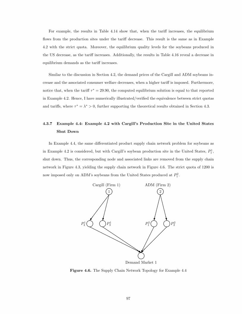
For example, the results in Table 4.14 show that, when the tariff increases, the equilibrium
flows from the production sites under the tariff decrease. This result is the same as in Example
4.2 with the strict quota. Moreover, the equilibrium quality levels for the soybeans produced in
the US decrease, as the tariff increases. Additionally, the results in Table 4.16 reveal a decrease in
equilibrium demands as the tariff increases.
Similar to the discussion in Section 4.2, the demand prices of the Cargill and ADM soybeans in-
crease and the associated consumer welfare decreases, when a higher tariff is imposed. Furthermore,
notice that, when the tariff τ∗ = 29.90, the computed equilibrium solution is equal to that reported
in Example 4.2. Hence, I have numerically illustrated/verified the equivalence between strict quotas
and tariffs, where τ∗ = λ∗ > 0, further supporting the theoretical results obtained in Section 4.3.
4.3.7 Example 4.4: Example 4.2 with Cargill’s Production Site in the United States
Shut Down
In Example 4.4, the same differentiated product supply chain network problem for soybeans as
in Example 4.2 is considered, but with Cargill’s soybean production site in the United States, P 11 ,
shut down. Thus, the corresponding node and associated links are removed from the supply chain
network in Figure 4.3, yielding the supply chain network in Figure 4.6. The strict quota of 1200 is
now imposed only on ADM’s soybeans from the United States produced at P 21 .
� ��1��������
�������/
Cargill (Firm 1) ADM (Firm 2)
� ��2��������
CCCCCCCW� ��P 1
2 � ��P 13 � ��P 2
1 � ��P 22
� ��
HHHHH
HHHHHH
HHHj
QQQQQQQQQQs
��������
��
��
���
Demand Market 1
Figure 4.6. The Supply Chain Network Topology for Example 4.4
97

I report the equilibrium soybean flows, in tons, the equilibrium quality levels, the equilibrium
demands for soybeans at Demand Market 1, and the average quality levels in Table 4.17 and Table
4.18.
Equilibrium Flows Results Equilibrium Quality ResultsQ∗111 - q∗11 -Q∗121 930.73 q∗12 100.00Q∗131 926.80 q∗13 100.00Q∗211 788.93 q∗21 100.00Q∗221 633.23 q∗22 99.36
Table 4.17. Equilibrium Product Flows and Equilibrium Quality Levels in Example 4.4
Demand Results Average Quality Resultsd∗11 1,857.53 q11 100.00d∗21 1,422.16 q21 98.38
Table 4.18. Equilibrium Demands and Average Quality in Example 4.4
Furthermore, the equilibrium Lagrange multiplier, which is the equivalent tariff, becomes:
λ∗ = 0.00.
Due to the shutdown of Cargill’s production site in the United States, its soybean flows from the
other sites, that are located in Brazil and Argentina, increase. Meanwhile, with less competition
from Cargill, ADM delivers more soybeans to China from the cheaper site, P 21 , in the United States,
and fewer soybeans from the more expensive site, P 22 , in Brazil. Since the strict quota is only
imposed on ADM in this example, there is more opportunity for ADM to increase its production
in the US. Furthermore, ADM’s soybean production in the US site does not meet the strict quota,
resulting in a zero equilibrium Lagrange multiplier.
The results for the computed equilibrium incurred demand prices per ton of soybeans of Cargill
and ADM at Demand Market 1, in dollars, the consumer welfare at the demand market, and the
profits achieved by Cargill and ADM, in dollars, are provided in Table 4.19.
Demand Price Results CW Results Profits Resultsρ11 728.31 CW11 517,560.59 U1 1,131,885.86ρ21 741.75 CW21 353,945.28 U2 756,415.15
Table 4.19. Equilibrium Demand Prices, Consumer Welfare, and Profits in Example 4.4
As compared to the results in Example 4.2, the quality levels of soybeans produced by Cargill,
including the average quality, increase to the maximum level, after its production site in the United
98
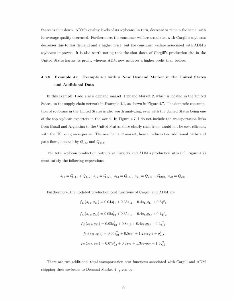
States is shut down. ADM’s quality levels of its soybeans, in turn, decrease or remain the same, with
its average quality decreased. Furthermore, the consumer welfare associated with Cargill’s soybeans
decreases due to less demand and a higher price, but the consumer welfare associated with ADM’s
soybeans improves. It is also worth noting that the shut down of Cargill’s production site in the
United States harms its profit, whereas ADM now achieves a higher profit than before.
4.3.8 Example 4.5: Example 4.1 with a New Demand Market in the United States
and Additional Data
In this example, I add a new demand market, Demand Market 2, which is located in the United
States, to the supply chain network in Example 4.1, as shown in Figure 4.7. The domestic consump-
tion of soybeans in the United States is also worth analyzing, even with the United States being one
of the top soybean exporters in the world. In Figure 4.7, I do not include the transportation links
from Brazil and Argentina to the United States, since clearly such trade would not be cost-efficient,
with the US being an exporter. The new demand market, hence, induces two additional paths and
path flows, denoted by Q112 and Q212.
The total soybean production outputs at Cargill’s and ADM’s production sites (cf. Figure 4.7)
must satisfy the following expressions:
s11 = Q111 +Q112, s12 = Q121, s13 = Q131, s21 = Q211 +Q212, s22 = Q221.
Furthermore, the updated production cost functions of Cargill and ADM are:
f11(s11, q11) = 0.04s211 + 0.35s11 + 0.4s11q11 + 0.6q211,
f12(s12, q12) = 0.05s212 + 0.35s12 + 0.4s12q12 + 0.4q212,
f13(s13, q13) = 0.05s213 + 0.8s13 + 0.4s13q13 + 0.4q213,
f21(s21, q21) = 0.06s221 + 0.5s21 + 1.2s21q21 + q221,
f22(s22, q22) = 0.07s222 + 0.3s22 + 1.3s22q22 + 1.5q222.
There are two additional total transportation cost functions associated with Cargill and ADM
shipping their soybeans to Demand Market 2, given by:
99
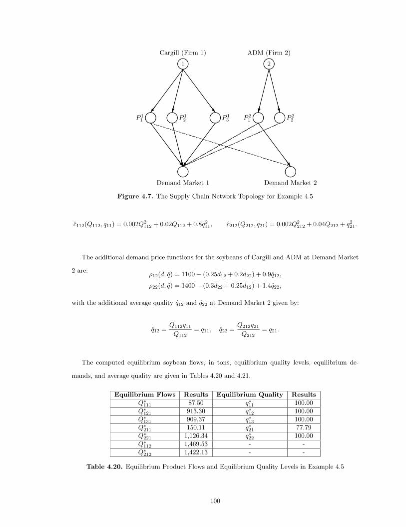
� ��1��������
�������/
SSSSSSSw
Cargill (Firm 1) ADM (Firm 2)
� ��2��������
CCCCCCCW� ��P 1
1 � ��P 12 � ��P 1
3 � ��P 21 � ��P 2
2
� ��
SSSSSSSw
CCCCCCCW
�������/ � ��
SSSSSSSw
Demand Market 1 Demand Market 2
Figure 4.7. The Supply Chain Network Topology for Example 4.5
c112(Q112, q11) = 0.002Q2112 + 0.02Q112 + 0.8q211, c212(Q212, q21) = 0.002Q2
212 + 0.04Q212 + q221.
The additional demand price functions for the soybeans of Cargill and ADM at Demand Market
2 are:ρ12(d, q) = 1100− (0.25d12 + 0.2d22) + 0.9q12,
ρ22(d, q) = 1400− (0.3d22 + 0.25d12) + 1.4q22,
with the additional average quality q12 and q22 at Demand Market 2 given by:
q12 =Q112q11Q112
= q11, q22 =Q212q21Q212
= q21.
The computed equilibrium soybean flows, in tons, equilibrium quality levels, equilibrium de-
mands, and average quality are given in Tables 4.20 and 4.21.
Equilibrium Flows Results Equilibrium Quality ResultsQ∗111 87.50 q∗11 100.00Q∗121 913.30 q∗12 100.00Q∗131 909.37 q∗13 100.00Q∗211 150.11 q∗21 77.79Q∗221 1,126.34 q∗22 100.00Q∗112 1,469.53 - -Q∗212 1,422.13 - -
Table 4.20. Equilibrium Product Flows and Equilibrium Quality Levels in Example 4.5
100
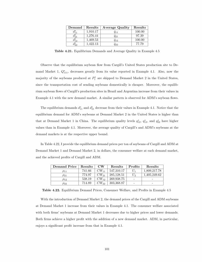
Demand Results Average Quality Resultsd∗11 1,910.17 q11 100.00d∗21 1,276.44 q21 97.39d∗12 1,469.53 q12 100.00d∗22 1,422.13 q22 77.79
Table 4.21. Equilibrium Demands and Average Quality in Example 4.5
Observe that the equilibrium soybean flow from Cargill’s United States production site to De-
mand Market 1, Q∗111, decreases greatly from its value reported in Example 4.1. Also, now the
majority of the soybeans produced at P 11 are shipped to Demand Market 2 in the United States,
since the transportation cost of sending soybeans domestically is cheaper. Moreover, the equilib-
rium soybean flows of Cargill’s production sites in Brazil and Argentina increase from their values in
Example 4.1 with the new demand market. A similar pattern is observed for ADM’s soybean flows.
The equilibrium demands d∗11 and d∗21 decrease from their values in Example 4.1. Notice that the
equilibrium demand for ADM’s soybeans at Demand Market 2 in the United States is higher than
that at Demand Market 1 in China. The equilibrium quality levels q∗12, q∗13, and q∗22 have higher
values than in Example 4.1. Moreover, the average quality of Cargill’s and ADM’s soybeans at the
demand markets is at the respective upper bound.
In Table 4.22, I provide the equilibrium demand prices per ton of soybeans of Cargill and ADM at
Demand Market 1 and Demand Market 2, in dollars, the consumer welfare at each demand market,
and the achieved profits of Cargill and ADM.
Demand Price Results CW Results Profits Resultsρ11 741.66 CW11 547,310.17 U1 1,809,217.78ρ21 774.97 CW21 285,128.51 U2 1,405,249.62ρ12 538.19 CW12 269,938.75 - -ρ22 714.89 CW22 303,368.87 - -
Table 4.22. Equilibrium Demand Prices, Consumer Welfare, and Profits in Example 4.5
With the introduction of Demand Market 2, the demand prices of the Cargill and ADM soybeans
at Demand Market 1 increase from their values in Example 4.1. The consumer welfare associated
with both firms’ soybeans at Demand Market 1 decreases due to higher prices and lower demands.
Both firms achieve a higher profit with the addition of a new demand market. ADM, in particular,
enjoys a significant profit increase from that in Example 4.1.
101
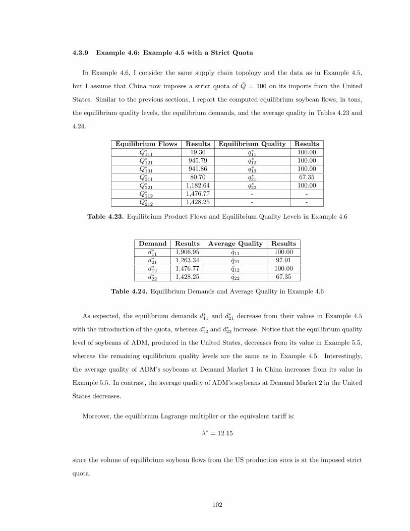
4.3.9 Example 4.6: Example 4.5 with a Strict Quota
In Example 4.6, I consider the same supply chain topology and the data as in Example 4.5,
but I assume that China now imposes a strict quota of Q = 100 on its imports from the United
States. Similar to the previous sections, I report the computed equilibrium soybean flows, in tons,
the equilibrium quality levels, the equilibrium demands, and the average quality in Tables 4.23 and
4.24.
Equilibrium Flows Results Equilibrium Quality ResultsQ∗111 19.30 q∗11 100.00Q∗121 945.79 q∗12 100.00Q∗131 941.86 q∗13 100.00Q∗211 80.70 q∗21 67.35Q∗221 1,182.64 q∗22 100.00Q∗112 1,476.77 - -Q∗212 1,428.25 - -
Table 4.23. Equilibrium Product Flows and Equilibrium Quality Levels in Example 4.6
Demand Results Average Quality Resultsd∗11 1,906.95 q11 100.00d∗21 1,263.34 q21 97.91d∗12 1,476.77 q12 100.00d∗22 1,428.25 q22 67.35
Table 4.24. Equilibrium Demands and Average Quality in Example 4.6
As expected, the equilibrium demands d∗11 and d∗21 decrease from their values in Example 4.5
with the introduction of the quota, whereas d∗12 and d∗22 increase. Notice that the equilibrium quality
level of soybeans of ADM, produced in the United States, decreases from its value in Example 5.5,
whereas the remaining equilibrium quality levels are the same as in Example 4.5. Interestingly,
the average quality of ADM’s soybeans at Demand Market 1 in China increases from its value in
Example 5.5. In contrast, the average quality of ADM’s soybeans at Demand Market 2 in the United
States decreases.
Moreover, the equilibrium Lagrange multiplier or the equivalent tariff is:
λ∗ = 12.15
since the volume of equilibrium soybean flows from the US production sites is at the imposed strict
quota.
102
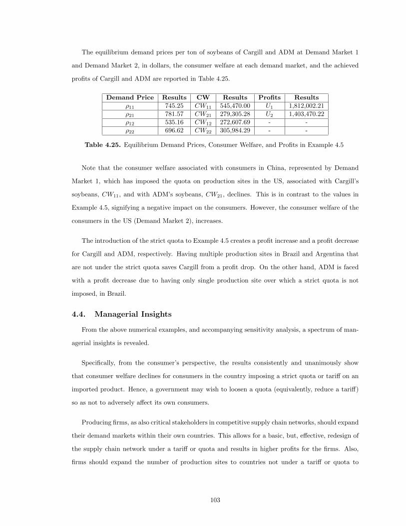
The equilibrium demand prices per ton of soybeans of Cargill and ADM at Demand Market 1
and Demand Market 2, in dollars, the consumer welfare at each demand market, and the achieved
profits of Cargill and ADM are reported in Table 4.25.
Demand Price Results CW Results Profits Resultsρ11 745.25 CW11 545,470.00 U1 1,812,002.21ρ21 781.57 CW21 279,305.28 U2 1,403,470.22ρ12 535.16 CW12 272,607.69 - -ρ22 696.62 CW22 305,984.29 - -
Table 4.25. Equilibrium Demand Prices, Consumer Welfare, and Profits in Example 4.5
Note that the consumer welfare associated with consumers in China, represented by Demand
Market 1, which has imposed the quota on production sites in the US, associated with Cargill’s
soybeans, CW11, and with ADM’s soybeans, CW21, declines. This is in contrast to the values in
Example 4.5, signifying a negative impact on the consumers. However, the consumer welfare of the
consumers in the US (Demand Market 2), increases.
The introduction of the strict quota to Example 4.5 creates a profit increase and a profit decrease
for Cargill and ADM, respectively. Having multiple production sites in Brazil and Argentina that
are not under the strict quota saves Cargill from a profit drop. On the other hand, ADM is faced
with a profit decrease due to having only single production site over which a strict quota is not
imposed, in Brazil.
4.4. Managerial Insights
From the above numerical examples, and accompanying sensitivity analysis, a spectrum of man-
agerial insights is revealed.
Specifically, from the consumer’s perspective, the results consistently and unanimously show
that consumer welfare declines for consumers in the country imposing a strict quota or tariff on an
imported product. Hence, a government may wish to loosen a quota (equivalently, reduce a tariff)
so as not to adversely affect its own consumers.
Producing firms, as also critical stakeholders in competitive supply chain networks, should expand
their demand markets within their own countries. This allows for a basic, but, effective, redesign of
the supply chain network under a tariff or quota and results in higher profits for the firms. Also,
firms should expand the number of production sites to countries not under a tariff or quota to
103
maintain or improve upon their profits if some of their production sites are in countries subject to
such trade policy instruments.
Finally, the examples numerically support the theoretical finding that a tariff has the equivalent
impact on product flows and product quality as a strict quota, provided that the tariff is set to the
Lagrange multiplier associated with the strict quota constraint and the constraint is tight. Hence,
governments have the flexibility of imposing either a tariff or a quota to obtain equivalent trade
flows and product quality levels. The imposition of a tariff may be more advisable/favored by a
government, since it requires less “policing” and also yields financial rewards.
4.5. Conclusions
Supply chain networks provide the pathways for the production and distribution of products to
consumers across the globe and serve as the critical infrastructure for world trade. Governments, in
their desire to influence world trade, utilize trade policies, in the form of quotas or tariffs. The recent
dynamism associated with the imposition of such policies worldwide merits closer attention from
modeling and computational perspectives. Although such topics have a long history in the economics
literature, they have been less explored in operations research / operations management, especially
from a supply chain perspective. Furthermore, the identification of the impacts on product quality
and how consumers are affected by such trade policy instruments, within the context of realistic
supply chain networks, is relevant for producers, consumers, and policy makers alike.
In this chapter, I add to the supply chain network, game theory, and trade policy literature by
constructing an oligopolistic supply chain network equilibrium model with differentiated products in
which firms have multiple production sites and multiple possible demand markets. The firms compete
in product quantities and product quality, subject to minimum quality standards, along with upper
bounds on quality. The model is then extended to include trade policy instruments in the form of a
strict quota or a tariff. I identify the governing equilibrium conditions, noting that the strict quota
model is characterized by a Generalized Nash Equilibrium, rather than a Nash Equilibrium, as is the
case of the other two models. I demonstrate that, nevertheless, the underlying equilibrium conditions
for all three models can be formulated and analyzed as an appropriate variational inequality problem,
for which an effective computational scheme is also provided, which yields closed form expressions
for the variables in each of the two steps of the procedure.
104
I establish theoretically, and also support the results numerically, that the equilibrium Lagrange
multiplier associated with the strict quota constraint in the strict quota model, if assigned as a tariff,
when the strict quota is tight, yields the same equilibrium product flows and product quality levels
for the tariff model as obtained for the quota model. This equivalence in a competitive supply chain
network allows decision-makers the option of using either a strict quota or a tariff to obtain identical
results. I also construct consumer welfare measures for the models.
In summary, the theoretical contributions in this chapter are the following:
1. The construction of the first general (not limited to a specific number of firms or demand markets
or functional forms) oligopolistic supply chain network equilibrium models with strategic variables
of quantities and product quality that incorporate multiple trade policy instruments;
2. The establishment of the equivalence of a tariff with that of a strict quota, provided that the
strict quota constraint is tight, and the Lagrange multiplier associated with it is the set tariff. This
provides decision-makers and policy makers, including governments, with the flexibility of imposing
either a tariff or a strict quota in practice.
3. The construction of a formula for the determination of the consumer welfare, under a tariff or
quota, in competitive supply chain networks.
4. The rigorous formulation of all the models as variational inequality problems, either with a tariff
or a strict quota, and with minimum and maximum quality bounds. In the case of the model with
a strict quota, the governing equilibrium conditions are those of a Generalized Nash Equilibrium,
because of the shared/common constraint. There are very few GNE supply chain models in the
literature to-date.
5. A proposed algorithm, with nice features for computations, for the new models, accompanied by
convergence conditions.
Illustrative examples are provided, along with numerical examples inspired by an important agri-
cultural product - that of soybeans. The numerical examples, accompanied by sensitivity analysis,
reveal that a government, in imposing trade policy instruments in the form of strict quotas or tar-
iffs, may decrease the welfare of its own consumers. The computational framework includes the
quantitative measurement of the impacts of a production site disruption as well as the addition of a
demand market.
105
In summary, the practical insights from this framework, are the following:
1. Governments should be cautious in imposing trade policy instruments in the form of tariffs or
quotas on products in competitive, that is, oligopolistic, supply chain networks, since the consumer
welfare of consumers in their own country can decrease as a result.
2. Governments, by imposing a tariff or quota, may help firms in their country garner enhanced
profits but at the expense of consumers.
3. Producers should expand the geographic dispersion of their production sites to reduce the impact
of imposed tariffs or quotas.
4. Producers should actively expand their demand markets in countries not under trade policy
instrument regimes, since doing so can lead to higher profits.
106
CHAPTER 5
QUALITY IN COMPETITIVE FRESH PRODUCE SUPPLY CHAINSWITH APPLICATION TO FARMERS’ MARKETS
According to a national survey conducted by Bond, Thilmany, and Bond (2009), four out of five
people living in the United States buy local food. Thus, the demand for locally grown fresh produce
is also increasing and demand and supply management becomes more crucial for farmers. A U.S.
Congressionally mandated report by the U.S. Department of Agriculture (cf. Low et al. (2015))
noted that the sale of food through direct-to-consumer channels, such as through farmers’ markets,
and intermediated marketing channels, that is, sales to institutions, including hospitals and schools,
or regional distributors, appears to be increasing. As reported therein, there were 8,268 farmers’
markets in the United States in 2014, with the number having increased by 180% since 2006. This
growth implies increasing consumer interest in locally sourced fresh produce due to quality and
health perspectives.
The majority of research on local food markets, especially farmers’ markets, pertains mostly
to consumer behavior and there are not many mathematical models that consider demand or the
supply side in local food supply chains. The literature on consumer behavior in farmers’ markets
provides valuable insights from the consumers’ and farms’ perspectives.
In this chapter, I develop a modeling and algorithmic framework for competitive farmers’ mar-
kets. The model is network-based and the farmers engage in Cournot competition over space and
time. The governing Nash equilibrium conditions are formulated as a variational inequality problem.
The novelty of the framework lies in that the quality of the fresh produce product is captured as
the produce propagates in the supply chain over space and time with the consumers at the mar-
kets responding both to the price and the quality of the fresh produce. Both uncapacitated and
capacitated versions of the model are presented. The latter can capture limitations in supply due to
harvest problems or damage during the growing season, limitations in transport and storage capa-
bilities, and/or labor for harvesting and processing. The game theory model can address questions
107
of farmers as to which farmers’ markets they should serve; what the impact of a new competitor
may be at one or more markets in terms of profits, as well as the effects of capacity disruptions
(or enhancements) in their individual and others’ short supply chains. In addition, the model can
ascertain the impacts of changes in link parameters that capture quality. Policy makers, in turn,
can also obtain useful information as to the impacts of a greater number or fewer farms represented
at various markets and how reducing quality decay can affect farmers’ profits.
The chapter is organized as follows. In Section 5.1, I provide some preliminaries, focusing on
the quality differential equations, which I then generalize to a path concept since the fresh produce
will proceed on multiple supply chain links from the harvesting point to ultimate purchase at the
farmers’ markets. Each link has associated with it both a time element as well as a factor such as
temperature, which also affects the fresh produce quality.
In Section 5.2, I first present the uncapacitated competitive supply chain network model for farm-
ers’ markets, give the governing Nash equilibrium conditions, and derive the variational inequality
formulations in path flows and links flows. In addition, I construct the capacitated path analogue
and provide its variational inequality formulation under Nash equilibrium. In Section 5.3, I present
the algorithm, which resolves the variational inequality problems into subproblems in the path flows
(and in the case of the capacitated model, also in terms of Lagrange multipliers) that can be solved
explicitly using formulae. In Section 5.4 a case study on apples in farmers’ markets is presented. I
summarize and present the conclusions in Section 5.5.
This chapter is based on the paper by Besik and Nagurney (2017).
5.1. Preliminaries on Food Quality Deterioration
Before I present the fresh food supply chain network model for farmers’ markets, it is important
to provide some preliminaries on the definition of quality, and the kinetics behind the quality decay,
since quality has major relevance for the fresh food industry. Afterwards, I provide the generalization
of the quality differential equations for fresh produce supply chain networks by capturing them
through the path concept.
Fresh foods are biological products, they deteriorate and, consequently, lose quality over time
(Schouten et al. (2004), Singh and Anderson (2004)). Thus, an understanding of the biochem-
ical/physicochemical reactions, which cause the deterioration, is necessary in order to be able to
present an explanation of the quality loss (Singh and Cadwallader (2004)). According to Taoukis
108
and Labuza (1989), the rate of quality deterioration can be given as a function of its microenviron-
ment, gas composition, relative humidity, and temperature.
In this regard, Labuza (1984) captures the quality decay of a food attribute, Q, over time t,
through the differential equation:
∂Q
∂t= kQn = Ae(−E/RT )Qn. (5.1)
Here, k is the reaction rate and is defined by the Arrhenius formula, Ae(−E/RT ), where A is a
pre-exponential constant, T is the temperature, E is the activation energy, and R is the universal
gas constant (Arrhenius (1889)). Moreover, n is the reaction order, which is a non-negative integer
and belongs to the set Z∗ = {0} ∪ Z+. In general, the quality decay function of the food attribute
can be shown in terms of its reaction order. When the reaction order n is zero, that is, ∂Q∂t = k, the
quality decay rate of the food attribute Q can be expressed as the function:
f0(Q) = −kt. (5.2)
Furthermore, assuming that the initial quality is known and given as Q0, the remaining quality
Qt at time t, can be defined by using the zero order quality decay function as in Tijskens and
Polderdijk (1996):
Qt = Q0 + f0(Q) = Q0 − kt. (5.3)
Recall that the reaction constant k can be written by the Arrhenius formula to show the rela-
tionship between temperature and quality decay explicitly. Furthermore, having the reaction order
be 1 – also referred to as a first order reaction – leads to an exponential function, which is observed
commonly in food quality decay (Tijskens and Polderdijk (1996)). This type of quality decay is
given by the expression:
f1(Q) = e−kt. (5.4)
Notice that, since this quality decay function has an exponential component, the quality Qt at
time t should be written as a multiplication of the initial quality Q0 and the quality decay function,
as shown in the following expression:
Qt = Q0f1(Q) = Q0e−kt. (5.5)
109
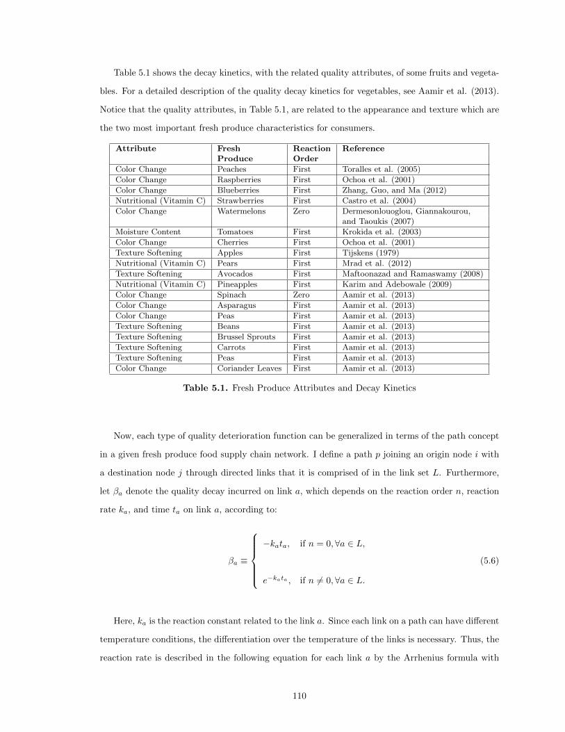
Table 5.1 shows the decay kinetics, with the related quality attributes, of some fruits and vegeta-
bles. For a detailed description of the quality decay kinetics for vegetables, see Aamir et al. (2013).
Notice that the quality attributes, in Table 5.1, are related to the appearance and texture which are
the two most important fresh produce characteristics for consumers.
Attribute Fresh Reaction ReferenceProduce Order
Color Change Peaches First Toralles et al. (2005)
Color Change Raspberries First Ochoa et al. (2001)
Color Change Blueberries First Zhang, Guo, and Ma (2012)
Nutritional (Vitamin C) Strawberries First Castro et al. (2004)
Color Change Watermelons Zero Dermesonlouoglou, Giannakourou,and Taoukis (2007)
Moisture Content Tomatoes First Krokida et al. (2003)
Color Change Cherries First Ochoa et al. (2001)
Texture Softening Apples First Tijskens (1979)
Nutritional (Vitamin C) Pears First Mrad et al. (2012)
Texture Softening Avocados First Maftoonazad and Ramaswamy (2008)
Nutritional (Vitamin C) Pineapples First Karim and Adebowale (2009)
Color Change Spinach Zero Aamir et al. (2013)
Color Change Asparagus First Aamir et al. (2013)
Color Change Peas First Aamir et al. (2013)
Texture Softening Beans First Aamir et al. (2013)
Texture Softening Brussel Sprouts First Aamir et al. (2013)
Texture Softening Carrots First Aamir et al. (2013)
Texture Softening Peas First Aamir et al. (2013)
Color Change Coriander Leaves First Aamir et al. (2013)
Table 5.1. Fresh Produce Attributes and Decay Kinetics
Now, each type of quality deterioration function can be generalized in terms of the path concept
in a given fresh produce food supply chain network. I define a path p joining an origin node i with
a destination node j through directed links that it is comprised of in the link set L. Furthermore,
let βa denote the quality decay incurred on link a, which depends on the reaction order n, reaction
rate ka, and time ta on link a, according to:
βa ≡
−kata, if n = 0,∀a ∈ L,
e−kata , if n 6= 0,∀a ∈ L.
(5.6)
Here, ka is the reaction constant related to the link a. Since each link on a path can have different
temperature conditions, the differentiation over the temperature of the links is necessary. Thus, the
reaction rate is described in the following equation for each link a by the Arrhenius formula with
110
the same parameters as in (5.1), except that the temperature is now denoted for each link a as Ta,
where:
ka = Ae(−EA/RTa). (5.7)
In addition, since (5.7) contains the exponential decay as a function and the other terms are
parameters, βa is defined generally for the reaction orders greater than zero. Before I show the
quality decay over a given path p, it is worthwhile to introduce the quality parameter q0i, which
represents the initial quality of the fresh produce, produced at the origin node i. Also, P ij represents
the set of all paths that have origin i and destination j. I now can define the quality qp, over a path
p, joining the origin farm node, i, with a destination node farmer market, j, while incorporating the
quality deterioration of the fresh produce as:
qp ≡
q0i +∑a∈p
βa, if n = 0,∀a ∈ L, p ∈ P ij ,∀i, j,
q0i∏a∈p
βa, if n = 1,∀a ∈ L, p ∈ P ij ,∀i, j.
(5.8)
By the above generalization, the model is differentiated from the existing works in the literature.
Although I utilize Tijskens and Polderdijk (1996)’s quality decay formulations, the authors have
not provided a quality deterioration formulation for a path in a food supply chain network. Rong,
Akkerman, and Grunow (2011) build the food supply chain through a mixed-integer programming
model and incorporate the food quality decay into this model. However, in this chapter, I present
a competitive supply chain game theory model where the demand markets and the quality decay
are product specific. Furthermore, Ketzenberg, Bloemhof, and Gaukler (2015) present a model
to assess the value of time and temperature information of a perishable product. The authors
provide a simulation study to evaluate the remaining shelf life of fresh fish with randomly realized
temperature and time information. In their work, they provide a different food quality metric than
the one presented in this chapter which is not based on quality kinetics and is not applied on a
supply chain network.
Next, the competitive fresh produce supply chain network model for farmers’ markets is pre-
sented.
111
5.2. The Fresh Produce Farmers’ Market Supply Chain Network Models
In this section, I capture the economic behavior of farmers selling at farmers’ markets and
competing on quality and quantity of their fresh produce a la Cournot (1838) through both an
uncapacitated and a capacitated oligopoly model and the variational inequality formulations of the
governing Nash (1950, 1951) equilibrium conditions are derived. The models consist of a finite
number of I farms, that are run by farmers, typically, denoted by i, and a finite number of demand
points, M , which correspond to farmers’ markets, and with a typical one denoted by j. Each farmers’
market takes place in a region and on a given day of the week. It is assumed that the demand points
correspond to farmers’ markets on different days of the week since farmers may not have sufficient
staff to be at multiple markets on the same day. Farmers’ markets, on any given day, usually last
no more than 6 hours and are repeated in the same location and day over a season, which, in the
Northeast of the United States, for example, can last from May through October.
The uncapacitated model is presented in Section 5.2.1 and its capacitated analogue then outlined
in Section 5.2.2.
Before introducing the variables and the notation for the models, I provide a summary of the
assumptions that are made:
1. The supply chain network topology illustrates a fixed time horizon in a given season of the
fresh fruit or vegetable, typically, a week.
2. The demand points represent the direct-to-consumer local farmers’ markets, in different regions
of a county or a state.
3. Farmers pick the harvest right before the beginning of the time horizon; therefore, a farmers’
market that is available at the beginning of this time horizon sells the fresh produce without
storage. Farmers’ markets taking place on subsequent days store the fresh produce before
transporting it to the markets.
4. Consumers can buy products that are substitutes of one other within or across the demand
points. That means that the farmers’ markets provide multiple options of fresh produce to
consumers over space and time.
Since the local supply chains are short, the intermediate activities can be defined as: harvesting,
processing and packaging, storage, and transportation. Farmers compete at the local farmers’ mar-
112
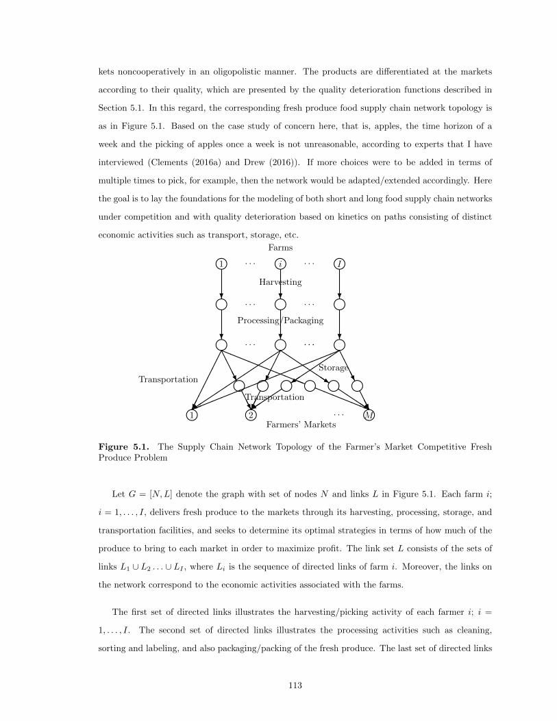
kets noncooperatively in an oligopolistic manner. The products are differentiated at the markets
according to their quality, which are presented by the quality deterioration functions described in
Section 5.1. In this regard, the corresponding fresh produce food supply chain network topology is
as in Figure 5.1. Based on the case study of concern here, that is, apples, the time horizon of a
week and the picking of apples once a week is not unreasonable, according to experts that I have
interviewed (Clements (2016a) and Drew (2016)). If more choices were to be added in terms of
multiple times to pick, for example, then the network would be adapted/extended accordingly. Here
the goal is to lay the foundations for the modeling of both short and long food supply chain networks
under competition and with quality deterioration based on kinetics on paths consisting of distinct
economic activities such as transport, storage, etc.
k k kk k k k k kk · · · k · · · k
1 2Farmers’ Markets
· · · M
· · ·
Storage
Transportation
Transportation
��������
AAAAU
AAAU
aaaaaaaaaaaaaaaa
��
��
���
���+
�����
����
QQQQQQs
QQQQs
AAAAU
AAAU
���
���+
��
��+
!!!!!!!!!!!!!!!!!
k k k? ? ?
Farmsk1 ki kIHarvesting
Processing/Packaging
? ? ?
· · · · · ·
· · · · · ·
Figure 5.1. The Supply Chain Network Topology of the Farmer’s Market Competitive FreshProduce Problem
Let G = [N,L] denote the graph with set of nodes N and links L in Figure 5.1. Each farm i;
i = 1, . . . , I, delivers fresh produce to the markets through its harvesting, processing, storage, and
transportation facilities, and seeks to determine its optimal strategies in terms of how much of the
produce to bring to each market in order to maximize profit. The link set L consists of the sets of
links L1 ∪ L2 . . . ∪ LI , where Li is the sequence of directed links of farm i. Moreover, the links on
the network correspond to the economic activities associated with the farms.
The first set of directed links illustrates the harvesting/picking activity of each farmer i; i =
1, . . . , I. The second set of directed links illustrates the processing activities such as cleaning,
sorting and labeling, and also packaging/packing of the fresh produce. The last set of directed links
113
corresponds to the storage and transport of the fresh produce. If the demand point is a farmers’
market that is open on the first day of the week, the links only capture the transportation cost.
Otherwise, there is a storage link followed by a transport link each subsequent demand point, that
is, farmers’ market, as illustrated in Figure 5.1.
Recall that P ij denotes the set of paths joining farm node i with farmer market node j. In
addition, P i denotes the set of paths emanating from farm node i to all farmer market nodes j;
j = 1, . . . ,M . P then denotes the set of all paths in the supply chain network in Figure 5.1. There
are nP paths in the network and nL links.
5.2.1 The Uncapacitated Model
The flow on each path, joining the farmer node i to the farmers’ market node j, is denoted by
xp, and all path flows must be nonnegative, that is,
xp ≥ 0, ∀p ∈ P ij ; i = 1, . . . , I; j = 1, . . . ,M. (5.9)
Furthermore, the flow on a link a is equal to the sum of the path flows xp, on paths that include
the link a. This conservation of flow equation is expressed as:
fa =∑p∈P
xpδap, ∀a ∈ L, (5.10)
where δap is equal to 1 if the link a is included in the path p, and 0, otherwise. In the local food
supply chain network, there is usually a single path between farm i and the market j; however, the
path set P ij is introduced to present a more general definition.
Furthermore, the demand at the farmers’ market j for the fresh produce product of farmer i is
given by: ∑p∈P i
j
xp = dij , p ∈ P ij ; i = 1, . . . , I; j = 1, . . . ,M. (5.11)
The demands between all farms and farmer market pairs (i, j) are grouped into the vector d and
also the quality of their fresh produce on paths p ∈ P ij , ∀i, j, {qp}, into the vector q. All vectors are
assumed to be column vectors.
The price of the product of farm i, in turn, at farmers’ market j, is denoted by ρij , and depends
not only on the demand for the farm’s fresh produce, but also on the quality of that product, which
114
is captured by the quality decay kinetics in (5.11). Also, the price depends, in general, on the
quantities of the competitors’ fresh produce at the markets as well as the quality of their products.
Hence, the demand price function ρij for farm i’s product at the farmers’ market j, is:
ρij = ρij(d, q), i = 1, . . . , I; j = 1, . . . ,M. (5.12)
In view of (5.11) and (5.12), the demand price functions can be rewritten as:
ρij = ρij(x, q) ≡ ρij(d, q), i = 1, . . . , I; j = 1, . . . ,M. (5.13)
The demand price functions are assumed to be continuous, continuously differentiable, and mono-
tone decreasing. Recall that the quality parameter vector q is defined with respect to the decay
function of the fresh produce which farms sell at the farmers’ markets and is time-dependent. Thus,
the demand price for a farm’s product is higher when the quality of its fresh produce product is
high and, if the demand is high, the price is lower. Note that each farm is aware of the temperature
conditions and the time associated with the links in its supply chain network.
The competition among the farms for resources is reflected in the total operational costs incurred
in harvesting, processing, storage, and transportation. The quality-keeping cost is related to the
food deterioration and is also considered through the transportation and the storage link costs. In
general, the total operational cost of each link a, denoted by ca, depends on the flows on all the
links in the fresh produce supply chain network, that is,
ca = ca(f), ∀a ∈ L, (5.14)
where f is the vector of all the link flows. The total cost on each link is assumed to be convex and
continuously differentiable.
Let Xi denote the vector of path flows associated with farm i; i = 1, . . . , I, where Xi ≡ {{xp}|p ∈
P i}} ∈ RnPi
+ , P i ≡ ∪j=1,...,MPij , and nP i denotes the number of paths from farm i to the farmers’
markets. Thus, X is the vector of all the farmers’ strategies, that is, X ≡ {{Xi}|i = 1, . . . , I}.
115
The profit function of farm i is defined as the difference between its revenue and its total costs,
where the total costs are the total operational costs over Li. The profit function is novel in terms of
capturing the quality of the fresh produce in the demand price functions, which is time-dependent.
The profit/utility function of farm i, denoted by Ui, is given by:
Ui =
M∑j=1
ρij(d, q)dij −∑a∈Li
ca(f). (5.15)
In lieu of the conservation of flow expressions (5.10) and (5.11), and the functional expressions
(5.13) and (5.14), Ui(X) ≡ Ui is defined for each farm i; i = 1, . . . , I, with the I-dimensional vector
U being the vector of the profits of all the farms with respect to their earnings at the farmers’
markets over a typical week:
U = U(X). (5.16)
Next, the fresh produce supply chain network Cournot-Nash Equilibrium conditions for farmers’
markets in a region are given.
• Definition 5.1: Fresh Produce Supply Chain Network Cournot-Nash Equilibrium
for Farmers’ Markets in the Uncapacitated Case
A path flow pattern X∗ ∈ K =∏Ii=1Ki constitutes a fresh produce supply chain network
Cournot-Nash equilibrium if for each farm i; i = 1, . . . , I:
Ui(X∗i , X
∗i ) ≥ Ui(Xi, X
∗i ), ∀Xi ∈ Ki, (5.17)
where X∗i ≡ (X∗1 , . . . , X∗i−1, X
∗i+1, . . . , X
∗I ) and Ki ≡ {Xi|Xi ∈ R
nPi
+ }. A Cournot-Nash
Equilibrium is established if no farm can unilaterally improve its profit by changing its product
flows throughout its supply chain network, given the product flow decisions of the other farms.
Next, the variational inequality formulations of the Cournot-Nash equilibrium for the fresh
produce supply chain network under oligopolistic competition satisfying Definition 5.1, in
terms of both path flows and link flows (see, e.g., Cournot (1838), Nash (1950, 1951), Gabay
and Moulin (1980), Nagurney (2006), and Nagurney et al. (2013)) are derived.
116
• Theorem 5.1: Variational Inequality Formulations of the Uncapacitated Model
Assume that for each fresh produce farm i; i = 1, . . . , I, the profit function Ui(X) is concave
with respect to the variables in Xi and is continuously differentiable. Then X∗ ∈ K is a
fresh produce supply chain network Cournot-Nash equilibrium for farmers’ markets according
to Definition 5.1 if and only if it satisfies the variational inequality:
−I∑i=1
〈∇XiUi(X∗), Xi −X∗i 〉 ≥ 0, ∀X ∈ K, (5.18)
where 〈·, ·〉 denotes the inner product in the corresponding Euclidean space and ∇XiUi(X)
denotes the gradient of Ui(X) with respect to Xi. Variational inequality (5.18), in turn, for
the uncapacitated model, is equivalent to the variational inequality that determines the vector
of equilibrium path flows x∗ ∈ K1 such that:
I∑i=1
M∑j=1
∑p∈P i
j
∂Cp(x∗)∂xp
− ρij(x∗, q)−M∑l=1
∂ρil(x∗, q)
∂xp
∑r∈P i
l
x∗r
× [xp − x∗p] ≥ 0, ∀x ∈ K1,
(5.19)
where K1 ≡ {x|x ∈ RnP+ }, and for each path p; p ∈ P ij ; i = 1, . . . , I; j = 1, . . . ,M ,
∂Cp(x)
∂xp≡∑a∈Li
∑b∈Li
∂cb(f)
∂faδap and
∂ρil(x, q)
∂xp≡ ∂ρil(d, q)
∂dij. (5.20)
Variational inequality (5.19) can also be rewritten in terms of link flows as: determine the
vector of equilibrium link flows and the vector of equilibrium demands (f∗, d∗) ∈ K2, such
that:I∑i=1
∑a∈Li
[∑b∈Li
∂cb(f∗)
∂fa
]× [fa − f∗a ]
+
I∑i=1
M∑j=1
[−ρij(d∗, q)−
M∑l=1
∂ρil(d∗, q)
∂dikd∗il
]× [dij − d∗ij ] ≥ 0, ∀(f, d) ∈ K2, (5.21)
where K2 ≡ {(f, d)|x ≥ 0, and (5.10) and (5.11) hold}.
Proof: (5.18) follows the discussion in Chapter 2. 2
117
Variational inequalities (5.19) and (5.21) can be put into standard form (see 2.1a): determine
X∗ ∈ K such that:
〈F (X∗), X −X∗〉 ≥ 0, ∀X ∈ K, (5.22)
where 〈·, ·〉 denotes the inner product in N -dimensional Euclidean space. Let X ≡ x and
F (X) ≡[∂Cp(x)
∂xp− ρij(x, q)−
M∑l=1
∂ρil(x, q)
∂xp
∑r∈P i
l
xr;
p ∈ P ij ; i = 1, . . . , I; j = 1, . . . ,M
], (5.23)
K ≡ K1, and N = nP , then (5.19) can be re-expressed as (5.22). Similarly, for the variational
inequality in terms of link flows, if the column vectors are defined: X ≡ (f, d) and F (X) ≡
(F1(X), F2(X)), where
F1(X) =
[∑b∈Li
∂cb(f)
∂fa; a ∈ Li; i = 1, . . . , I
],
F2(X) =
−ρij(x, q)− M∑l=1
∂ρil(x, q)
∂xp
∑r∈P i
l
xr; p ∈ P ij ; i = 1, . . . , I; j = 1, . . . ,M
, (5.24)
K ≡ K2, and N = nL +M , then (5.21) can be re-written as (5.22).
Since the feasible set K1 is not compact, and the same holds for K2, the existence of a solution
cannot be obtained simply based on the assumption of the continuity of F . However, the demand
dij for each farm i’s product; i = 1, . . . , I, at every farmers’ market j; j = 1, . . . ,M , may be assumed
to be bounded, since the population requiring these products is finite (although it may be large).
Consequently, in light of (5.12), the following is valid:
Kc ≡ {x| 0 ≤ x ≤ c, }, (5.25)
where c > 0 and x ≤ c means that xp ≤ c for all p ∈ P ij ; i = 1, . . . , I, and j = 1, . . . ,M . Then Kc is
a bounded, closed, and convex subset of K1. Thus, the following variational inequality
〈F (Xc), X −Xc〉 ≥ 0, ∀X ∈ Kc, (5.26)
admits at least one solution Xc ∈ Kc, since Kc is compact and F is continuous. Therefore, the
following theorem for existence in Chapter 2 is immediate:
118
• Theorem 5.2: Existence
There exists at least one solution to variational inequality (5.19) (equivalently, to (5.21)), since
there exists a c > 0, such that variational inequality (5.29) admits a solution in Kc with
xc ≤ c. (5.27)
In addition, I now provide a uniqueness result.
• Theorem 5.3: Uniqueness
With Theorem 5.2, variational inequality (5.26) and, hence, variational inequalities (5.19) and
(5.21) admit at least one solution. Moreover, if the function F (X) of variational inequality
(5.21), as defined in (5.22), is strictly monotone on K ≡ K2, that is,
〈(F (X1)− F (X2)), X1 −X2〉 > 0, ∀X1, X2 ∈ K, X1 6= X2, (5.28)
then the solution to variational inequality (5.21) is unique, that is, the equilibrium link flow
pattern and the equilibrium demand pattern are unique.
5.2.2 The Capacitated Model
In this subsection, I provide the capacitated version of the model in Section 5.2.1.
Specifically, I retain the objective function (5.15), for each farm i; i = 1, . . . , I, the nonnegativity
constraints (5.9), with conservation of flow equations (5.11), as well as the previous notation, but
now it becomes
fa ≤ ua, ∀a ∈ L, (5.29a)
or, in view of (5.10): ∑p∈P
xpδap ≤ ua, ∀a ∈ L, (5.29b)
where ua is the positive upper bound on the flow on link a.
The feasible set K3i faced by farm i in the capacitated case is defined as: K3
i ≡ {Xi|Xi ∈
RnPi
+ and (5.29b) holds for a ∈ Li}. Also, K3 ≡∏Ii=1K
3i is given.
Hence, the following definition is immediate.
119
• Definition 5.2: Fresh Produce Supply Chain Network Cournot-Nash Equilibrium
for Farmers’ Markets in the Capacitated Case
A path flow pattern X∗ ∈ K3 constitutes a fresh produce supply chain network Cournot-Nash
equilibrium in the capacitated case if for each farm i; i = 1, . . . , I:
Ui(X∗i , X
∗i ) ≥ Ui(Xi, X
∗i ), ∀Xi ∈ K3
i , (5.30)
where, as before, X∗i ≡ (X∗1 , . . . , X∗i−1, X
∗i+1, . . . , X
∗I )
• Theorem 5.4: Variational Inequality Formulations of the Capacitated Model
Assume that for each fresh produce farm i; i = 1, . . . , I, the profit function Ui(X) is concave
with respect to the variables in Xi, and is continuously differentiable. Then X∗ ∈ K3 is a fresh
produce supply chain network Cournot-Nash equilibrium for farmers’ markets in the capacitated
case according to Definition 2 if and only if it satisfies the variational inequality:
−I∑i=1
〈∇XiUi(X∗), Xi −X∗i 〉 ≥ 0, ∀X ∈ K3. (5.31)
Variational inequality (5.31), in turn, for the capacitated model, is equivalent to the variational
inequality that determines the vector of equilibrium path flows x∗ ∈ K3 such that:
I∑i=1
M∑j=1
∑p∈P i
j
∂Cp(x∗)∂xp
− ρij(x∗, q)−M∑l=1
∂ρil(x∗, q)
∂xp
∑r∈P i
l
x∗r
× [xp − x∗p] ≥ 0, ∀x ∈ K3.
(5.32)
Moreover, variational inequality (5.32) is equivalent to the variational inequality problem: de-
termine (x∗, λ∗) ∈ K4, where K4 ≡ {x ∈ RnP+ , λ ∈ RnL
+ }, such that:
I∑i=1
M∑j=1
∑p∈P i
j
∂Cp(x∗)∂xp
− ρij(x∗, q)−M∑l=1
∂ρil(x∗, q)
∂xp
∑r∈P i
l
x∗r +∑a∈L
λ∗aδap
× [xp − x∗p]
+∑a∈L
ua −∑p∈P
x∗pδap
× [λa − λ∗a] ≥ 0, ∀(x, λ) ∈ K4, (5.33)
where∂Cp(x)∂xp
and ∂ρil(x,q)∂xp
are as defined in (5.20).
120
Proof: Variational inequality (5.31) again follows directly from Gabay and Moulin (1980). Vari-
ational inequality (5.33) follows, in turn, from Bertsekas and Tsitsiklis (1989) (see also Nagurney
(2010)) with notice that λ∗ corresponds to the vector of optimal Lagrange multipliers associated
with constraints (5.29b) and λ is the vector of Lagrange multipliers associated with the upper
bound constraints on all links a ∈ L.
Variational inequality (5.33) will be used for solution of the capacitated model and note that
variational inequality (5.33) can be put into the standard form (5.22) (see Nagurney (1999) and
Chapter 2), if the vectors: X ≡ (x, λ) and F (X) ≡ (F3(X), F4(X)), where
F3(X) =
∂Cp(x)
∂xp− ρij(x, q)−
M∑l=1
∂ρil(x, q)
∂xp
∑r∈P i
l
xr +∑a∈L
λaδap, p ∈ P ij ; i = 1, . . . , I; j = 1, . . . ,M
,(5.34)
F4(X) =
ua −∑p∈P
xpδap, a ∈ L
. (5.35)
With K ≡ K4, (5.33) can be rewritten as (5.22).
The existence result below follows from the classical theory of variational inequalities (see Chapter
2).
• Theorem 5.5: Existence of a Solution to the Capacitated Model
Existence of a solution X∗ to variational inequality (5.31) is guaranteed since the feasible set
K3 is compact.
5.3. The Algorithm
I now present the explicit formulae for recall the Euler method to compute the solution of the
capacitated and uncapacitated models in Section 5.2. The details on the Euler method are provided
in Chapter 2.
5.3.1 Explicit Formulae for the Euler Method Applied to the Uncapacitated Model
The elegance of this procedure for the computation of solutions to the uncapacitated fresh produce
farmers’ market supply chain network problem in Section 5.2.1 can be seen in the following explicit
121
formulae. In particular, the following closed form expressions for the fresh produce path flows are
written, for each path p ∈ P ij , ∀i, j:
xτ+1p = max{0, xτp + aτ (ρij(x
τ , q) +
M∑l=1
∂ρil(xτ , q)
∂xp
∑r∈P i
l
xτr −∂Cp(x
τ )
∂xp)},
∀p ∈ P ij ; i = 1, . . . , I; j = 1, . . . ,M. (5.36)
Next, the closed form expression to compute the solution of the capacitated problem in Section
5.2.2 is given.
5.3.2 Explicit Formulae for the Euler Method Applied to the Capacitated Model
The explicit formulae are now given to compute the solutions to the capacitated fresh produce
farmers’ market supply chain problem in Section 5.2.2. The closed form expressions for the fresh
produce path flows at iteration τ + 1 are as follows. For each path p ∈ P ij , ∀i, j, compute:
xτ+1p = max{0, xτp + aτ (ρij(x
τ , q) +
M∑l=1
∂ρil(xτ , q)
∂xp
∑r∈P i
l
xτr −∂Cp(x
τ )
∂xp−∑a∈L
λτaδap)},
∀p ∈ P ij ; i = 1, . . . , I; j = 1, . . . ,M. (5.37)
The Lagrange multipliers for each link a ∈ Li; i = 1, . . . , I, can be computed as:
λτ+1a = max{0, λτa + aτ (
∑p∈P
xτpδap − ua)}, ∀a ∈ L. (5.38)
The number of strategic variables xp, as well as the number of the paths, in the supply chain network,
for both of the uncapacitated and capacitated supply chain networks, grow linearly in terms of the
number of nodes in the supply chain network, be it a farm, or a farmers’ market, etc. Therefore,
even a fresh produce supply chain network with hundreds of demand markets is still tractable within
the proposed modeling and computational framework.
5.4. Case Study
I focus on apples for the case study. The United States holds second place in the world’s apple
production with 4 million metric tons of apples produced, with the leader being China, which
produced 33 million metric tons of apples in 2010 (USDA (2012)). Specifically, in the case study
122
I consider Golden Delicious apples. This type of apple is ranked in third place among the other
apple varieties in the United States with 25,000 metric tons of production value. The case study
is based on farmers’ markets in western Massachusetts in the United States. According to the
USDA (2016) and the website of Community Involved in Sustaining Agriculture (CISA), there are
8,558 farmers markets in the United States, 312 in Massachusetts, and 40 in western Massachusetts
(CISA (2016)). Also, in Massachusetts, 369 in-state apple orchards produced 34 million pounds of
apples in 2010. There are approximately 27 apple orchards in western Massachusetts. For this case
study, I selected three of the apple orchards located in western Massachusetts: Apex Orchards, the
Park Hill Orchard, and Sentinel Farm. The locations of these orchards/farms in Massachusetts are,
respectively, Shelburne, Easthampton, and Belchertown. These orchards/farms have the possibility
of selling their apples at the Amherst, Northampton, South Hadley, and/or Belchertown farmers’
markets, which are open on different days in a given week during the season, as shown in Figure
5.2. The Northampton Farmers’ Market is open on Tuesdays, the South Hadley Farmers’ Market
operates on Thursdays. On Saturdays the Amherst Farmers’ Market is open, and the Belchertown
Farmers’ Market is open on Sundays. Each orchard/farm has its own harvesting, processing, storage,
and transportation units. Notice that the demand points in Figure 5.2 are sequenced depending on
the day of the week. For example, since the Northampton Farmers’ Market is open on Tuesdays,
which is the first farmers’ market of the week in this case study, it is numbered as the first demand
point. The South Hadley Farmers’ Market corresponds to demand point 2, and so on. Additionally,
apples are picked on Tuesdays at all the orchards/farms, so that there is no storage for the Golden
Delicious apples sold at the Northampton Farmers’ Market. However, each farm should store its
Golden Delicious apples for 2, 4, and 5 days for the South Hadley, Amherst, and the Belchertown
Farmers’ Markets, respectively.
The Euler method for the uncapacitated (cf. (5.36)) and the capacitated problems (cf. (5.38) and
(5.39)) is implemented in MATLAB and the sequence aτ = {1, 12 ,12 ,
13 , . . .}, with the convergence
tolerance being 10−6, that is, the Euler method is deemed to have converged if the absolute value
of the difference of each successive variable iterate differs by no more than this value. The code in
Matlab is executed on a Macbook Pro laptop with a 2.8 GHz Intel Core i5 processor and 8GB 1600
MHz DDR3 memory.
123
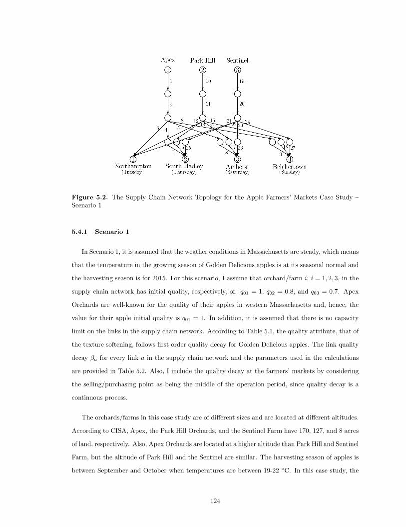
Figure 5.2. The Supply Chain Network Topology for the Apple Farmers’ Markets Case Study –Scenario 1
5.4.1 Scenario 1
In Scenario 1, it is assumed that the weather conditions in Massachusetts are steady, which means
that the temperature in the growing season of Golden Delicious apples is at its seasonal normal and
the harvesting season is for 2015. For this scenario, I assume that orchard/farm i; i = 1, 2, 3, in the
supply chain network has initial quality, respectively, of: q01 = 1, q02 = 0.8, and q03 = 0.7. Apex
Orchards are well-known for the quality of their apples in western Massachusetts and, hence, the
value for their apple initial quality is q01 = 1. In addition, it is assumed that there is no capacity
limit on the links in the supply chain network. According to Table 5.1, the quality attribute, that of
the texture softening, follows first order quality decay for Golden Delicious apples. The link quality
decay βa for every link a in the supply chain network and the parameters used in the calculations
are provided in Table 5.2. Also, I include the quality decay at the farmers’ markets by considering
the selling/purchasing point as being the middle of the operation period, since quality decay is a
continuous process.
The orchards/farms in this case study are of different sizes and are located at different altitudes.
According to CISA, Apex, the Park Hill Orchards, and the Sentinel Farm have 170, 127, and 8 acres
of land, respectively. Also, Apex Orchards are located at a higher altitude than Park Hill and Sentinel
Farm, but the altitude of Park Hill and the Sentinel are similar. The harvesting season of apples is
between September and October when temperatures are between 19-22 ◦C. In this case study, the
124
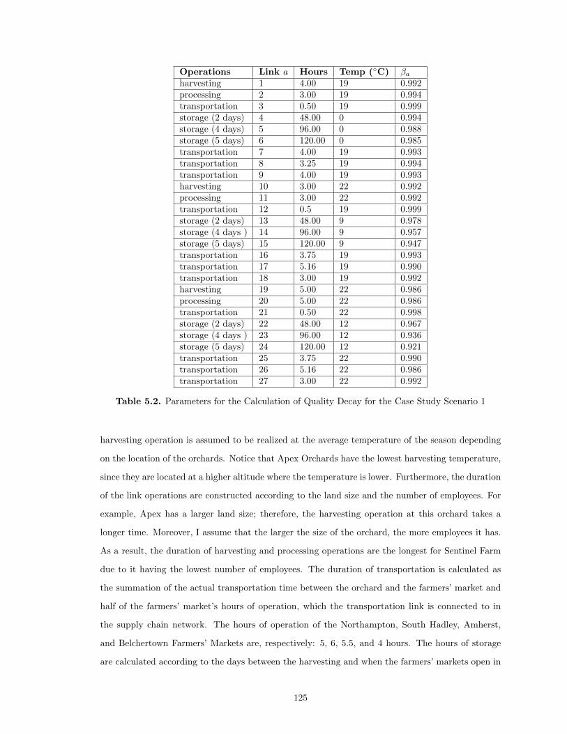
Operations Link a Hours Temp (◦C) βaharvesting 1 4.00 19 0.992processing 2 3.00 19 0.994transportation 3 0.50 19 0.999storage (2 days) 4 48.00 0 0.994storage (4 days) 5 96.00 0 0.988storage (5 days) 6 120.00 0 0.985transportation 7 4.00 19 0.993transportation 8 3.25 19 0.994transportation 9 4.00 19 0.993harvesting 10 3.00 22 0.992processing 11 3.00 22 0.992transportation 12 0.5 19 0.999storage (2 days) 13 48.00 9 0.978storage (4 days ) 14 96.00 9 0.957storage (5 days) 15 120.00 9 0.947transportation 16 3.75 19 0.993transportation 17 5.16 19 0.990transportation 18 3.00 19 0.992harvesting 19 5.00 22 0.986processing 20 5.00 22 0.986transportation 21 0.50 22 0.998storage (2 days) 22 48.00 12 0.967storage (4 days ) 23 96.00 12 0.936storage (5 days) 24 120.00 12 0.921transportation 25 3.75 22 0.990transportation 26 5.16 22 0.986transportation 27 3.00 22 0.992
Table 5.2. Parameters for the Calculation of Quality Decay for the Case Study Scenario 1
harvesting operation is assumed to be realized at the average temperature of the season depending
on the location of the orchards. Notice that Apex Orchards have the lowest harvesting temperature,
since they are located at a higher altitude where the temperature is lower. Furthermore, the duration
of the link operations are constructed according to the land size and the number of employees. For
example, Apex has a larger land size; therefore, the harvesting operation at this orchard takes a
longer time. Moreover, I assume that the larger the size of the orchard, the more employees it has.
As a result, the duration of harvesting and processing operations are the longest for Sentinel Farm
due to it having the lowest number of employees. The duration of transportation is calculated as
the summation of the actual transportation time between the orchard and the farmers’ market and
half of the farmers’ market’s hours of operation, which the transportation link is connected to in
the supply chain network. The hours of operation of the Northampton, South Hadley, Amherst,
and Belchertown Farmers’ Markets are, respectively: 5, 6, 5.5, and 4 hours. The hours of storage
are calculated according to the days between the harvesting and when the farmers’ markets open in
125
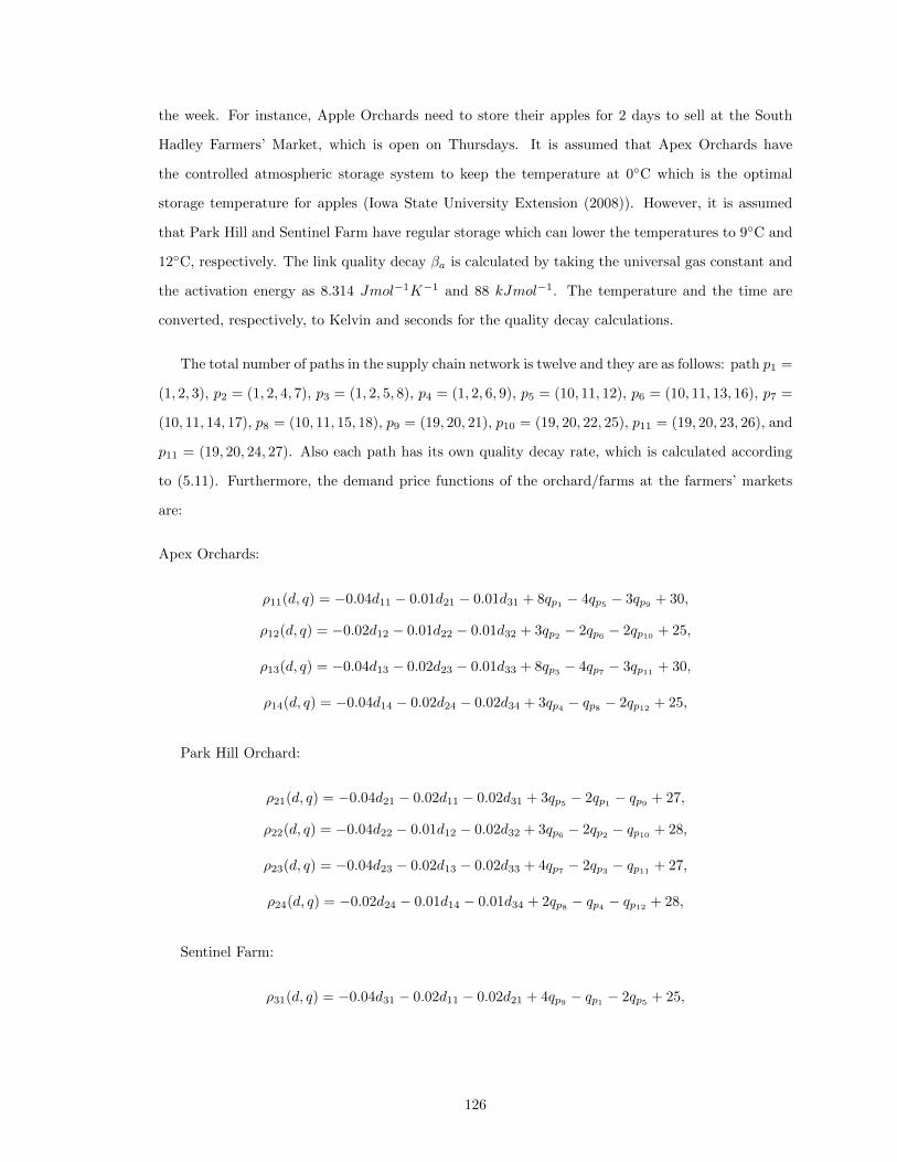
the week. For instance, Apple Orchards need to store their apples for 2 days to sell at the South
Hadley Farmers’ Market, which is open on Thursdays. It is assumed that Apex Orchards have
the controlled atmospheric storage system to keep the temperature at 0◦C which is the optimal
storage temperature for apples (Iowa State University Extension (2008)). However, it is assumed
that Park Hill and Sentinel Farm have regular storage which can lower the temperatures to 9◦C and
12◦C, respectively. The link quality decay βa is calculated by taking the universal gas constant and
the activation energy as 8.314 Jmol−1K−1 and 88 kJmol−1. The temperature and the time are
converted, respectively, to Kelvin and seconds for the quality decay calculations.
The total number of paths in the supply chain network is twelve and they are as follows: path p1 =
(1, 2, 3), p2 = (1, 2, 4, 7), p3 = (1, 2, 5, 8), p4 = (1, 2, 6, 9), p5 = (10, 11, 12), p6 = (10, 11, 13, 16), p7 =
(10, 11, 14, 17), p8 = (10, 11, 15, 18), p9 = (19, 20, 21), p10 = (19, 20, 22, 25), p11 = (19, 20, 23, 26), and
p11 = (19, 20, 24, 27). Also each path has its own quality decay rate, which is calculated according
to (5.11). Furthermore, the demand price functions of the orchard/farms at the farmers’ markets
are:
Apex Orchards:
ρ11(d, q) = −0.04d11 − 0.01d21 − 0.01d31 + 8qp1 − 4qp5 − 3qp9 + 30,
ρ12(d, q) = −0.02d12 − 0.01d22 − 0.01d32 + 3qp2 − 2qp6 − 2qp10 + 25,
ρ13(d, q) = −0.04d13 − 0.02d23 − 0.01d33 + 8qp3 − 4qp7 − 3qp11 + 30,
ρ14(d, q) = −0.04d14 − 0.02d24 − 0.02d34 + 3qp4 − qp8 − 2qp12 + 25,
Park Hill Orchard:
ρ21(d, q) = −0.04d21 − 0.02d11 − 0.02d31 + 3qp5 − 2qp1 − qp9 + 27,
ρ22(d, q) = −0.04d22 − 0.01d12 − 0.02d32 + 3qp6 − 2qp2 − qp10 + 28,
ρ23(d, q) = −0.04d23 − 0.02d13 − 0.02d33 + 4qp7 − 2qp3 − qp11 + 27,
ρ24(d, q) = −0.02d24 − 0.01d14 − 0.01d34 + 2qp8 − qp4 − qp12 + 28,
Sentinel Farm:
ρ31(d, q) = −0.04d31 − 0.02d11 − 0.02d21 + 4qp9 − qp1 − 2qp5 + 25,
126
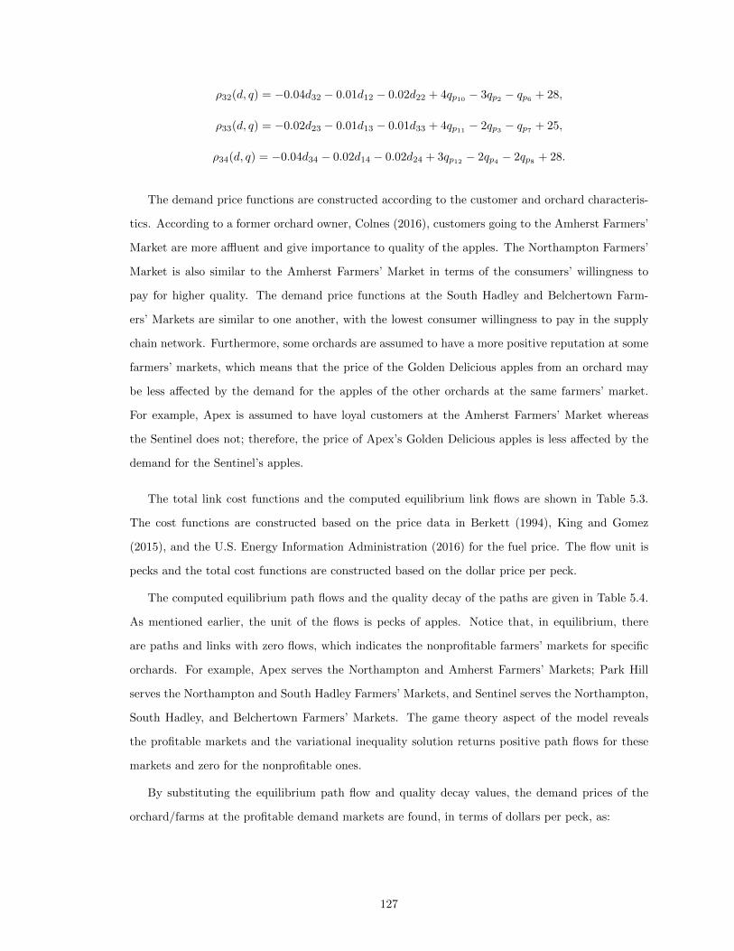
ρ32(d, q) = −0.04d32 − 0.01d12 − 0.02d22 + 4qp10 − 3qp2 − qp6 + 28,
ρ33(d, q) = −0.02d23 − 0.01d13 − 0.01d33 + 4qp11 − 2qp3 − qp7 + 25,
ρ34(d, q) = −0.04d34 − 0.02d14 − 0.02d24 + 3qp12 − 2qp4 − 2qp8 + 28.
The demand price functions are constructed according to the customer and orchard characteris-
tics. According to a former orchard owner, Colnes (2016), customers going to the Amherst Farmers’
Market are more affluent and give importance to quality of the apples. The Northampton Farmers’
Market is also similar to the Amherst Farmers’ Market in terms of the consumers’ willingness to
pay for higher quality. The demand price functions at the South Hadley and Belchertown Farm-
ers’ Markets are similar to one another, with the lowest consumer willingness to pay in the supply
chain network. Furthermore, some orchards are assumed to have a more positive reputation at some
farmers’ markets, which means that the price of the Golden Delicious apples from an orchard may
be less affected by the demand for the apples of the other orchards at the same farmers’ market.
For example, Apex is assumed to have loyal customers at the Amherst Farmers’ Market whereas
the Sentinel does not; therefore, the price of Apex’s Golden Delicious apples is less affected by the
demand for the Sentinel’s apples.
The total link cost functions and the computed equilibrium link flows are shown in Table 5.3.
The cost functions are constructed based on the price data in Berkett (1994), King and Gomez
(2015), and the U.S. Energy Information Administration (2016) for the fuel price. The flow unit is
pecks and the total cost functions are constructed based on the dollar price per peck.
The computed equilibrium path flows and the quality decay of the paths are given in Table 5.4.
As mentioned earlier, the unit of the flows is pecks of apples. Notice that, in equilibrium, there
are paths and links with zero flows, which indicates the nonprofitable farmers’ markets for specific
orchards. For example, Apex serves the Northampton and Amherst Farmers’ Markets; Park Hill
serves the Northampton and South Hadley Farmers’ Markets, and Sentinel serves the Northampton,
South Hadley, and Belchertown Farmers’ Markets. The game theory aspect of the model reveals
the profitable markets and the variational inequality solution returns positive path flows for these
markets and zero for the nonprofitable ones.
By substituting the equilibrium path flow and quality decay values, the demand prices of the
orchard/farms at the profitable demand markets are found, in terms of dollars per peck, as:
127
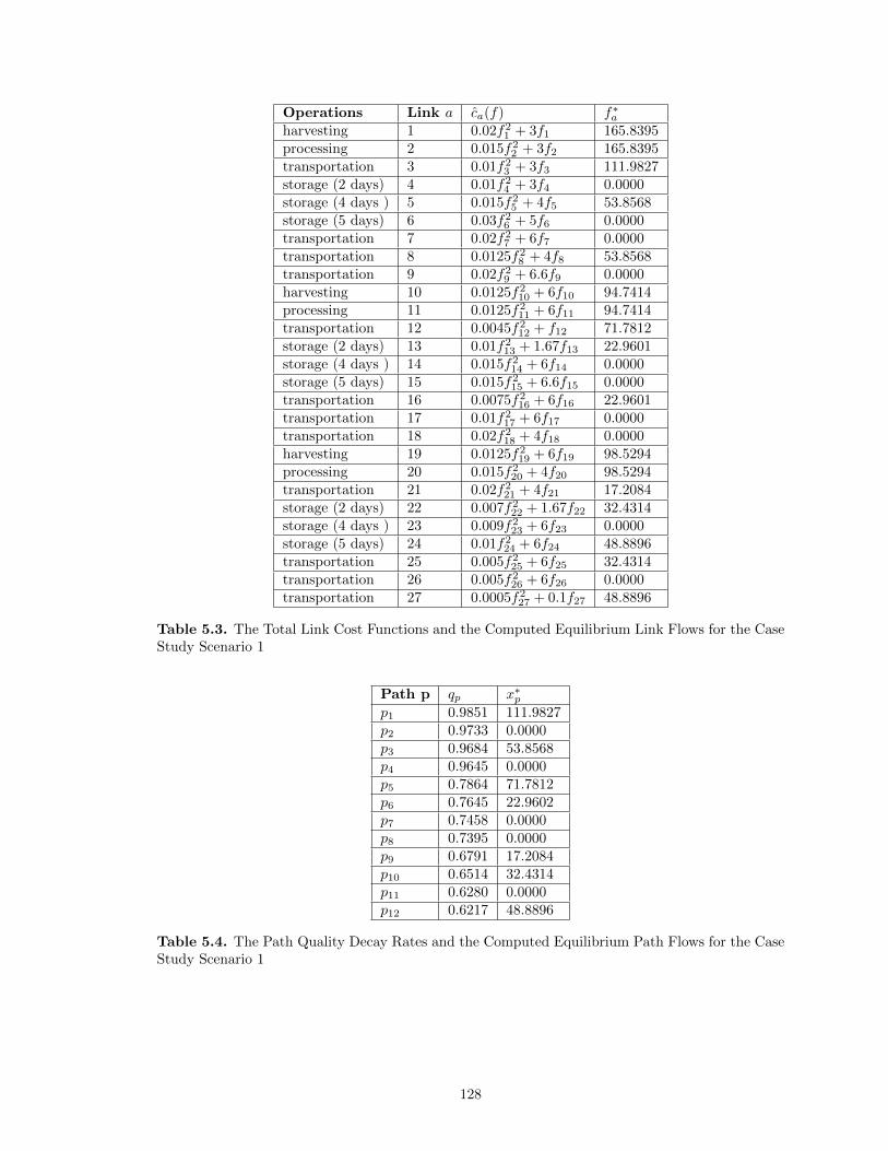
Operations Link a ca(f) f∗aharvesting 1 0.02f21 + 3f1 165.8395processing 2 0.015f22 + 3f2 165.8395transportation 3 0.01f23 + 3f3 111.9827storage (2 days) 4 0.01f24 + 3f4 0.0000storage (4 days ) 5 0.015f25 + 4f5 53.8568storage (5 days) 6 0.03f26 + 5f6 0.0000transportation 7 0.02f27 + 6f7 0.0000transportation 8 0.0125f28 + 4f8 53.8568transportation 9 0.02f29 + 6.6f9 0.0000harvesting 10 0.0125f210 + 6f10 94.7414processing 11 0.0125f211 + 6f11 94.7414transportation 12 0.0045f212 + f12 71.7812storage (2 days) 13 0.01f213 + 1.67f13 22.9601storage (4 days ) 14 0.015f214 + 6f14 0.0000storage (5 days) 15 0.015f215 + 6.6f15 0.0000transportation 16 0.0075f216 + 6f16 22.9601transportation 17 0.01f217 + 6f17 0.0000transportation 18 0.02f218 + 4f18 0.0000harvesting 19 0.0125f219 + 6f19 98.5294processing 20 0.015f220 + 4f20 98.5294transportation 21 0.02f221 + 4f21 17.2084storage (2 days) 22 0.007f222 + 1.67f22 32.4314storage (4 days ) 23 0.009f223 + 6f23 0.0000storage (5 days) 24 0.01f224 + 6f24 48.8896transportation 25 0.005f225 + 6f25 32.4314transportation 26 0.005f226 + 6f26 0.0000transportation 27 0.0005f227 + 0.1f27 48.8896
Table 5.3. The Total Link Cost Functions and the Computed Equilibrium Link Flows for the CaseStudy Scenario 1
Path p qp x∗pp1 0.9851 111.9827p2 0.9733 0.0000p3 0.9684 53.8568p4 0.9645 0.0000p5 0.7864 71.7812p6 0.7645 22.9602p7 0.7458 0.0000p8 0.7395 0.0000p9 0.6791 17.2084p10 0.6514 32.4314p11 0.6280 0.0000p12 0.6217 48.8896
Table 5.4. The Path Quality Decay Rates and the Computed Equilibrium Path Flows for the CaseStudy Scenario 1
128
Apex Orchards:
ρ11 = 27.33, ρ12 = 24.53, ρ13 = 30.72, ρ14 = 25.42,
Park Hill Orchard:
ρ21 = 21.25, ρ22 = 26.13, ρ23 = 26.34, ρ24 = 27.40,
Sentinel Farm:
ρ31 = 20.79, ρ32 = 25.16, ρ33 = 24.29, ρ34 = 24.50.
According to Clements (2016), who is an educator at the University of Massachusetts Amherst
Extension Fruit Program, the retail price of Golden Delicious apples is usually $2 per pound. A
peck of apples is equal to 10-12 pounds which means the price of a peck can be between $20-$24.
The results for the demand prices are close to this range and, hence, are consistent with reality.
Furthermore, the profits of the orchard/farms, in dollars, at the equilibrium solution, are:
U1(X∗) = 1785.40, U2(X∗) = 484.03, U3(X∗) = 460.15.
Apex Orchards have the largest profit in Scenario 1, followed by Park Hill Orchard and then the
Sentinel Farm.
5.4.2 Scenario 2
In this scenario, it is assumed that a new orchard, which was solely selling to retailers and whole-
salers previously, is attracted by the demand for apples at the farmers’ markets. This hypothetical
new orchard is called New Orchard, and is located in western Massachusetts and enters the local food
supply chain as depicted in Figure 5.3. As in Scenario 1, the uncapacitated variational inequality
problem (5.22) is solved with the Euler method, using the explicit formulae shown in (5.37).
The quality decay parameters and the link quality decay rates of New Orchard are shown in
Table 5.5 and the total link cost functions are depicted in Table 5.6. The initial quality for this
orchard is, q04 = 1, and the other orchard/farms have the same initial quality values as in Scenario
1. New Orchard is very similar to Apex Orchards in terms of its land size, the number of employees,
and the storage technology. Therefore, the New Orchards’ total link cost functions for harvesting,
processing, and storage are very similar to those of Apex. It is assumed that New Orchard is located
129
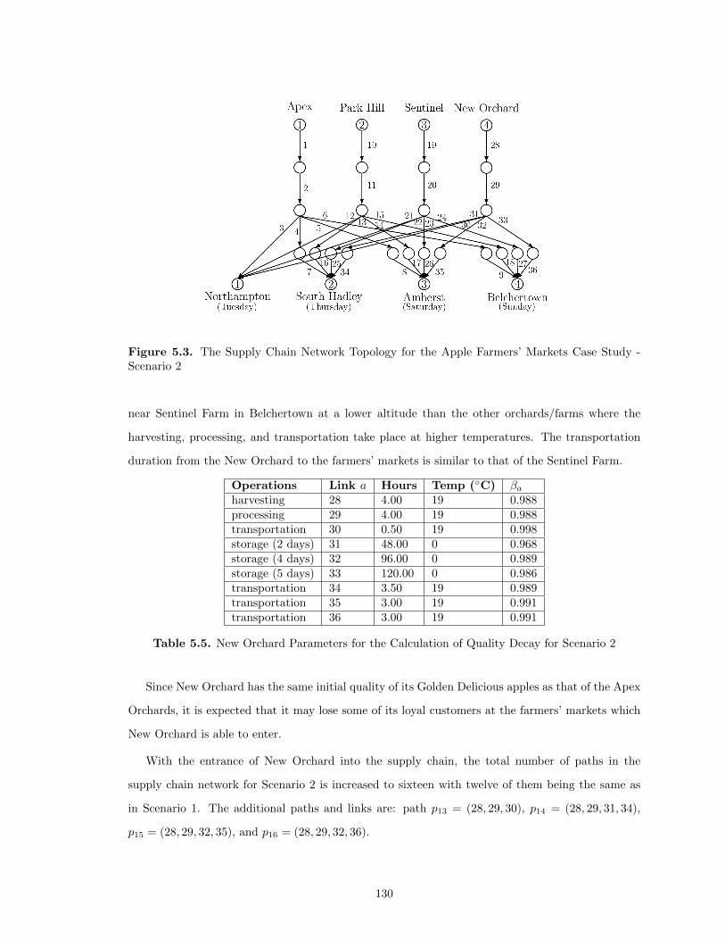
Figure 5.3. The Supply Chain Network Topology for the Apple Farmers’ Markets Case Study -Scenario 2
near Sentinel Farm in Belchertown at a lower altitude than the other orchards/farms where the
harvesting, processing, and transportation take place at higher temperatures. The transportation
duration from the New Orchard to the farmers’ markets is similar to that of the Sentinel Farm.
Operations Link a Hours Temp (◦C) βaharvesting 28 4.00 19 0.988processing 29 4.00 19 0.988transportation 30 0.50 19 0.998storage (2 days) 31 48.00 0 0.968storage (4 days) 32 96.00 0 0.989storage (5 days) 33 120.00 0 0.986transportation 34 3.50 19 0.989transportation 35 3.00 19 0.991transportation 36 3.00 19 0.991
Table 5.5. New Orchard Parameters for the Calculation of Quality Decay for Scenario 2
Since New Orchard has the same initial quality of its Golden Delicious apples as that of the Apex
Orchards, it is expected that it may lose some of its loyal customers at the farmers’ markets which
New Orchard is able to enter.
With the entrance of New Orchard into the supply chain, the total number of paths in the
supply chain network for Scenario 2 is increased to sixteen with twelve of them being the same as
in Scenario 1. The additional paths and links are: path p13 = (28, 29, 30), p14 = (28, 29, 31, 34),
p15 = (28, 29, 32, 35), and p16 = (28, 29, 32, 36).
130
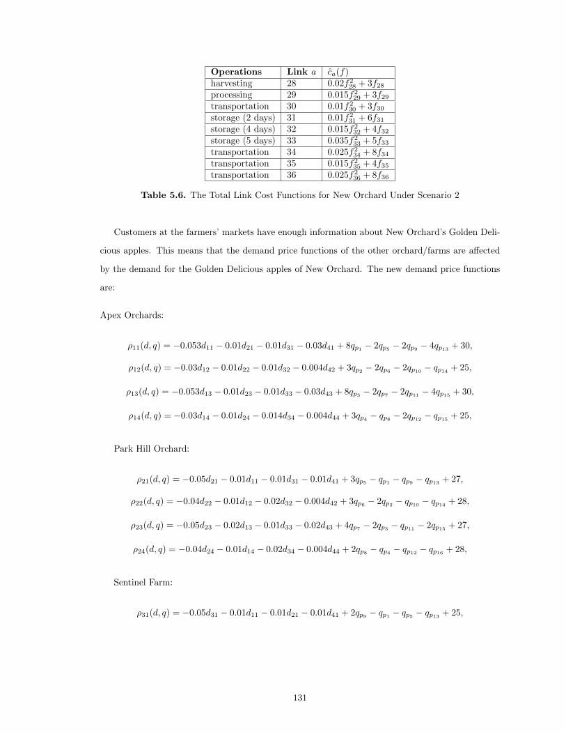
Operations Link a ca(f)harvesting 28 0.02f228 + 3f28processing 29 0.015f229 + 3f29transportation 30 0.01f230 + 3f30storage (2 days) 31 0.01f231 + 6f31storage (4 days) 32 0.015f232 + 4f32storage (5 days) 33 0.035f233 + 5f33transportation 34 0.025f234 + 8f34transportation 35 0.015f235 + 4f35transportation 36 0.025f236 + 8f36
Table 5.6. The Total Link Cost Functions for New Orchard Under Scenario 2
Customers at the farmers’ markets have enough information about New Orchard’s Golden Deli-
cious apples. This means that the demand price functions of the other orchard/farms are affected
by the demand for the Golden Delicious apples of New Orchard. The new demand price functions
are:
Apex Orchards:
ρ11(d, q) = −0.053d11 − 0.01d21 − 0.01d31 − 0.03d41 + 8qp1 − 2qp5 − 2qp9 − 4qp13 + 30,
ρ12(d, q) = −0.03d12 − 0.01d22 − 0.01d32 − 0.004d42 + 3qp2 − 2qp6 − 2qp10 − qp14 + 25,
ρ13(d, q) = −0.053d13 − 0.01d23 − 0.01d33 − 0.03d43 + 8qp3 − 2qp7 − 2qp11 − 4qp15 + 30,
ρ14(d, q) = −0.03d14 − 0.01d24 − 0.014d34 − 0.004d44 + 3qp4 − qp8 − 2qp12 − qp15 + 25,
Park Hill Orchard:
ρ21(d, q) = −0.05d21 − 0.01d11 − 0.01d31 − 0.01d41 + 3qp5 − qp1 − qp9 − qp13 + 27,
ρ22(d, q) = −0.04d22 − 0.01d12 − 0.02d32 − 0.004d42 + 3qp6 − 2qp2 − qp10 − qp14 + 28,
ρ23(d, q) = −0.05d23 − 0.02d13 − 0.01d33 − 0.02d43 + 4qp7 − 2qp3 − qp11 − 2qp15 + 27,
ρ24(d, q) = −0.04d24 − 0.01d14 − 0.02d34 − 0.004d44 + 2qp8 − qp4 − qp12 − qp16 + 28,
Sentinel Farm:
ρ31(d, q) = −0.05d31 − 0.01d11 − 0.01d21 − 0.01d41 + 2qp9 − qp1 − qp5 − qp13 + 25,
131
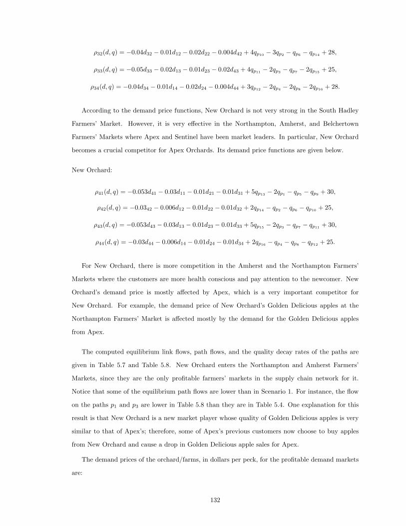
ρ32(d, q) = −0.04d32 − 0.01d12 − 0.02d22 − 0.004d42 + 4qp10 − 3qp2 − qp6 − qp14 + 28,
ρ33(d, q) = −0.05d33 − 0.02d13 − 0.01d23 − 0.02d43 + 4qp11 − 2qp3 − qp7 − 2qp15 + 25,
ρ34(d, q) = −0.04d34 − 0.01d14 − 0.02d24 − 0.004d44 + 3qp12 − 2qp4 − 2qp8 − 2qp16 + 28.
According to the demand price functions, New Orchard is not very strong in the South Hadley
Farmers’ Market. However, it is very effective in the Northampton, Amherst, and Belchertown
Farmers’ Markets where Apex and Sentinel have been market leaders. In particular, New Orchard
becomes a crucial competitor for Apex Orchards. Its demand price functions are given below.
New Orchard:
ρ41(d, q) = −0.053d41 − 0.03d11 − 0.01d21 − 0.01d31 + 5qp13 − 2qp1 − qp5 − qp9 + 30,
ρ42(d, q) = −0.0342 − 0.006d12 − 0.01d22 − 0.01d32 + 2qp14 − qp2 − qp6 − qp10 + 25,
ρ43(d, q) = −0.053d43 − 0.03d13 − 0.01d23 − 0.01d33 + 5qp15 − 2qp3 − qp7 − qp11 + 30,
ρ44(d, q) = −0.03d44 − 0.006d14 − 0.01d24 − 0.01d34 + 2qp16 − qp4 − qp8 − qp12 + 25.
For New Orchard, there is more competition in the Amherst and the Northampton Farmers’
Markets where the customers are more health conscious and pay attention to the newcomer. New
Orchard’s demand price is mostly affected by Apex, which is a very important competitor for
New Orchard. For example, the demand price of New Orchard’s Golden Delicious apples at the
Northampton Farmers’ Market is affected mostly by the demand for the Golden Delicious apples
from Apex.
The computed equilibrium link flows, path flows, and the quality decay rates of the paths are
given in Table 5.7 and Table 5.8. New Orchard enters the Northampton and Amherst Farmers’
Markets, since they are the only profitable farmers’ markets in the supply chain network for it.
Notice that some of the equilibrium path flows are lower than in Scenario 1. For instance, the flow
on the paths p1 and p3 are lower in Table 5.8 than they are in Table 5.4. One explanation for this
result is that New Orchard is a new market player whose quality of Golden Delicious apples is very
similar to that of Apex’s; therefore, some of Apex’s previous customers now choose to buy apples
from New Orchard and cause a drop in Golden Delicious apple sales for Apex.
The demand prices of the orchard/farms, in dollars per peck, for the profitable demand markets
are:
132
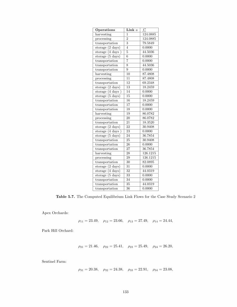
Operations Link a f∗aharvesting 1 124.0885
processing 2 124.0885
transportation 3 79.5849
storage (2 days) 4 0.0000
storage (4 days ) 5 44.5036
storage (5 days) 6 0.0000
transportation 7 0.0000
transportation 8 44.5036
transportation 9 0.0000
harvesting 10 87.4808
processing 11 87.4808
transportation 12 69.2348
storage (2 days) 13 18.2459
storage (4 days ) 14 0.0000
storage (5 days) 15 0.0000
transportation 16 18.2459
transportation 17 0.0000
transportation 18 0.0000
harvesting 19 86.0782
processing 20 86.0782
transportation 21 18.3520
storage (2 days) 22 30.9408
storage (4 days ) 23 0.0000
storage (5 days) 24 36.7854
transportation 25 30.9408
transportation 26 0.0000
transportation 27 36.7854
harvesting 28 126.1215
processing 29 126.1215
transportation 30 82.0895
storage (2 days) 31 0.0000
storage (4 days) 32 44.0319
storage (5 days) 33 0.0000
transportation 34 0.0000
transportation 35 44.0319
transportation 36 0.0000
Table 5.7. The Computed Equilibrium Link Flows for the Case Study Scenario 2
Apex Orchards:
ρ11 = 23.49, ρ12 = 23.66, ρ13 = 27.49, ρ14 = 24.44,
Park Hill Orchard:
ρ21 = 21.46, ρ22 = 25.41, ρ23 = 25.49, ρ24 = 26.20,
Sentinel Farm:
ρ31 = 20.38, ρ32 = 24.38, ρ33 = 22.91, ρ34 = 23.08,
133
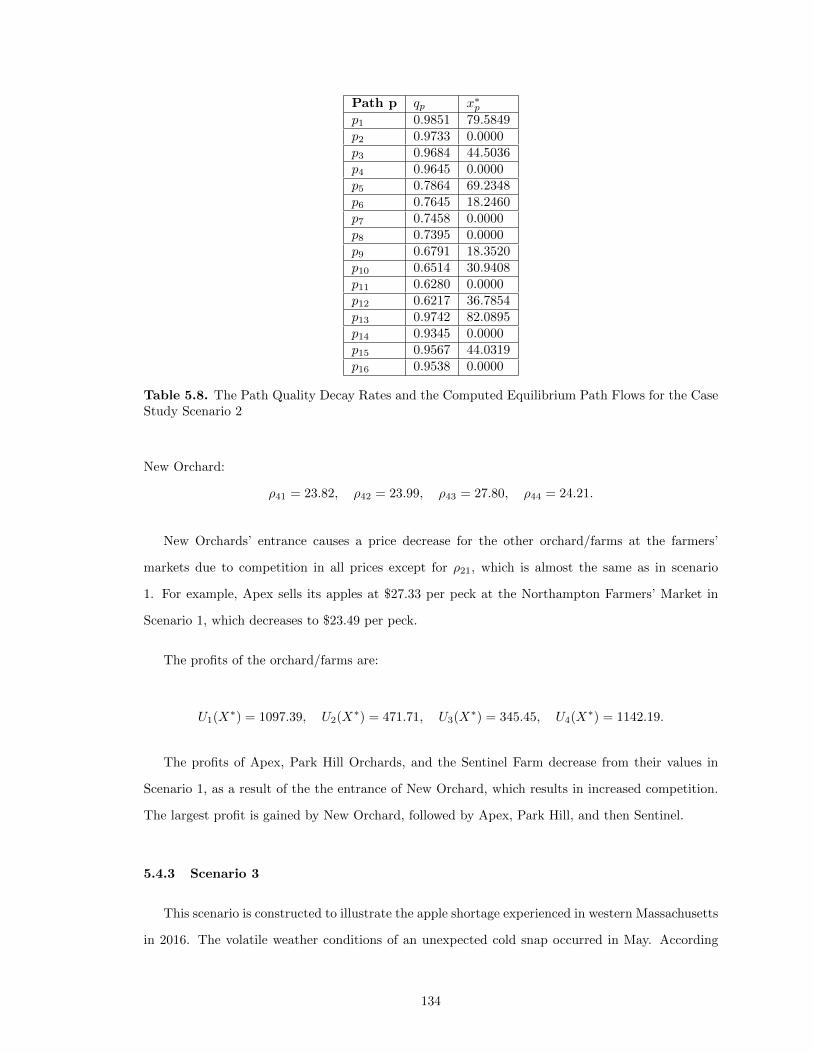
Path p qp x∗pp1 0.9851 79.5849p2 0.9733 0.0000p3 0.9684 44.5036p4 0.9645 0.0000p5 0.7864 69.2348p6 0.7645 18.2460p7 0.7458 0.0000p8 0.7395 0.0000p9 0.6791 18.3520p10 0.6514 30.9408p11 0.6280 0.0000p12 0.6217 36.7854p13 0.9742 82.0895p14 0.9345 0.0000p15 0.9567 44.0319p16 0.9538 0.0000
Table 5.8. The Path Quality Decay Rates and the Computed Equilibrium Path Flows for the CaseStudy Scenario 2
New Orchard:
ρ41 = 23.82, ρ42 = 23.99, ρ43 = 27.80, ρ44 = 24.21.
New Orchards’ entrance causes a price decrease for the other orchard/farms at the farmers’
markets due to competition in all prices except for ρ21, which is almost the same as in scenario
1. For example, Apex sells its apples at $27.33 per peck at the Northampton Farmers’ Market in
Scenario 1, which decreases to $23.49 per peck.
The profits of the orchard/farms are:
U1(X∗) = 1097.39, U2(X∗) = 471.71, U3(X∗) = 345.45, U4(X∗) = 1142.19.
The profits of Apex, Park Hill Orchards, and the Sentinel Farm decrease from their values in
Scenario 1, as a result of the the entrance of New Orchard, which results in increased competition.
The largest profit is gained by New Orchard, followed by Apex, Park Hill, and then Sentinel.
5.4.3 Scenario 3
This scenario is constructed to illustrate the apple shortage experienced in western Massachusetts
in 2016. The volatile weather conditions of an unexpected cold snap occurred in May. According
134
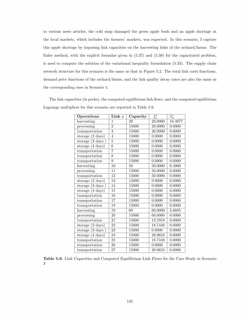
to various news articles, the cold snap damaged the green apple buds and an apple shortage at
the local markets, which includes the farmers’ markets, was expected. In this scenario, I capture
this apple shortage by imposing link capacities on the harvesting links of the orchard/farms. The
Euler method, with the explicit formulae given in (5.37) and (5.38) for the capacitated problem,
is used to compute the solution of the variational inequality formulation (5.33). The supply chain
network structure for this scenario is the same as that in Figure 5.2. The total link costs functions,
demand price functions of the orchard/farms, and the link quality decay rates are also the same as
the corresponding ones in Scenario 1.
The link capacities (in pecks), the computed equilibrium link flows, and the computed equilibrium
Lagrange multipliers for this scenario are reported in Table 5.9.
Operations Link a Capacity f∗a λ∗aharvesting 1 20 20.0000 16.4077processing 2 15000 20.0000 0.0000transportation 3 15000 20.0000 0.0000storage (2 days) 4 15000 0.0000 0.0000storage (3 days ) 5 15000 0.0000 0.0000storage (4 days) 6 15000 0.0000 0.0000transportation 7 15000 0.0000 0.0000transportation 8 15000 0.0000 0.0000transportation 9 15000 0.0000 0.0000harvesting 10 50 50.0000 6.4906processing 11 15000 50.0000 0.0000transportation 12 15000 50.0000 0.0000storage (2 days) 13 15000 0.0000 0.0000storage (3 days ) 14 15000 0.0000 0.0000storage (4 days) 15 15000 0.0000 0.0000transportation 16 15000 0.0000 0.0000transportation 17 15000 0.0000 0.0000transportation 18 15000 0.0000 0.0000harvesting 19 60 60.0000 5.6685processing 20 15000 60.0000 0.0000transportation 21 15000 13.1918 0.0000storage (2 days) 22 15000 18.7448 0.0000storage (3 days ) 23 15000 0.0000 0.0000storage (4 days) 24 15000 28.0624 0.0000transportation 25 15000 18.7448 0.0000transportation 26 15000 0.0000 0.0000transportation 27 15000 28.0624 0.0000
Table 5.9. Link Capacities and Computed Equilibrium Link Flows for the Case Study in Scenario3
135
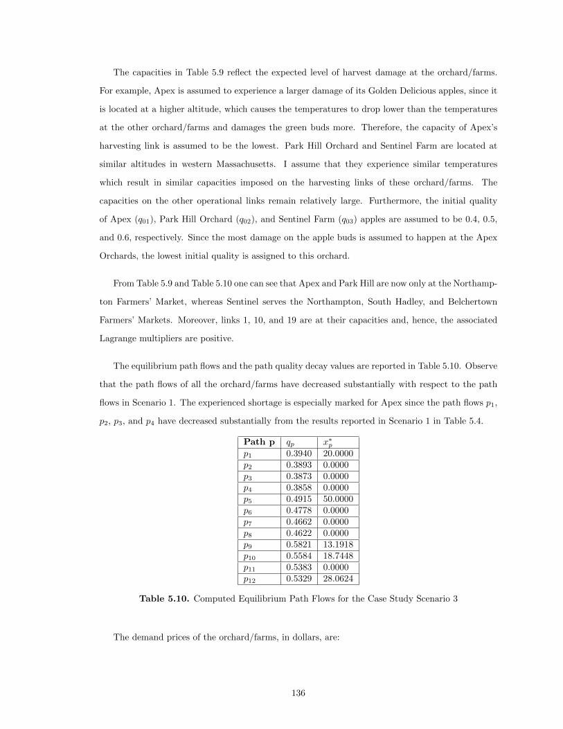
The capacities in Table 5.9 reflect the expected level of harvest damage at the orchard/farms.
For example, Apex is assumed to experience a larger damage of its Golden Delicious apples, since it
is located at a higher altitude, which causes the temperatures to drop lower than the temperatures
at the other orchard/farms and damages the green buds more. Therefore, the capacity of Apex’s
harvesting link is assumed to be the lowest. Park Hill Orchard and Sentinel Farm are located at
similar altitudes in western Massachusetts. I assume that they experience similar temperatures
which result in similar capacities imposed on the harvesting links of these orchard/farms. The
capacities on the other operational links remain relatively large. Furthermore, the initial quality
of Apex (q01), Park Hill Orchard (q02), and Sentinel Farm (q03) apples are assumed to be 0.4, 0.5,
and 0.6, respectively. Since the most damage on the apple buds is assumed to happen at the Apex
Orchards, the lowest initial quality is assigned to this orchard.
From Table 5.9 and Table 5.10 one can see that Apex and Park Hill are now only at the Northamp-
ton Farmers’ Market, whereas Sentinel serves the Northampton, South Hadley, and Belchertown
Farmers’ Markets. Moreover, links 1, 10, and 19 are at their capacities and, hence, the associated
Lagrange multipliers are positive.
The equilibrium path flows and the path quality decay values are reported in Table 5.10. Observe
that the path flows of all the orchard/farms have decreased substantially with respect to the path
flows in Scenario 1. The experienced shortage is especially marked for Apex since the path flows p1,
p2, p3, and p4 have decreased substantially from the results reported in Scenario 1 in Table 5.4.
Path p qp x∗pp1 0.3940 20.0000p2 0.3893 0.0000p3 0.3873 0.0000p4 0.3858 0.0000p5 0.4915 50.0000p6 0.4778 0.0000p7 0.4662 0.0000p8 0.4622 0.0000p9 0.5821 13.1918p10 0.5584 18.7448p11 0.5383 0.0000p12 0.5329 28.0624
Table 5.10. Computed Equilibrium Path Flows for the Case Study Scenario 3
The demand prices of the orchard/farms, in dollars, are:
136
Apex Orchards:
ρ11 = 28.01, ρ12 = 23.91, ρ13 = 29.62, ρ14 = 24.35.
Park Hill Orchard:
ρ21 = 24.44, ρ22 = 27.72, ρ23 = 27.55, ρ24 = 27.72,
Sentinel Farm:
ρ31 = 24.02, ρ32 = 27.84, ρ33 = 25.91, ρ34 = 26.78.
Since the supply is decreased, the prices of Golden Delicious apples increase in most of the
farmers’ markets. For example, Apex’s Golden Delicious apples are now $28.01 at the Northampton
Farmers’ Market in this scenario whereas the price was $27.33 in Scenario 1. Additionally, since the
quality of Apex’s apples is worse than in Scenario 1, this causes the demand price to decrease at the
Amherst Farmers’ Market. In Scenario 1, the price of its apples at the Amherst Farmers’ Market
was $30.72; however, now it is $29.62.
The profits of the orchard/farms in this scenario, in dollars, are:
U1(X∗) = 362.15, U2(X∗) = 498.28, U3(X∗) = 507.58.
The largest profit is achieved by Sentinel, followed by Park Hill, and Apex. In Scenario 1, Apex
has the largest profit, which decreases substantially in this scenario due to it having the lowest
harvesting capacity and quality.
5.5. Summary and Conclusions
Fresh produce consists of both fruits and vegetables and such supply chains are especially chal-
lenging since the quality of the product deteriorates continuously upon harvesting. At the same time,
consumers are demanding fresh products and are increasingly health conscious. Farmers’ markets
have increased in popularity internationally and, yet, the mathematical modeling associated with
such supply chains has been limited.
In this chapter, I provide explicit formulae for a variety of fresh produce to capture quality
deterioration. I then identify the quality associated with different pathways in supply chain networks.
Subsequently, I focus on farmers’ markets, which are examples of direct to consumer supply chains
and are shorter supply chains since farmers bring the product to markets at which consumers select
137
their purchases. Specifically, I introduce a game theory model for supply chain competition in a
network framework for farmers’ markets occurring within a period of time, such as a week. The farms
are interested in maximizing their profits and the consumers respond to the quality of the product.
I provide both qualitative properties of the equilibrium link flow pattern, propose a computational
scheme, and also illustrate my framework through numerical examples focused on peaches and then
in a case study for Golden Delicious apples and farmers’ markets in western Massachusetts. The
mathematical framework considers both uncapacitated links in the supply chain network as well as
capacitated ones, which may occur due to crop failures, harvesting problems, labor shortages, etc.
This is the first game theory model for farmers’ markets and also the first competitive fresh produce
supply chain network model in which quality deterioration of fresh produce is explicitly captured.
138
CHAPTER 6
DYNAMICS OF QUALITY AS A STRATEGIC VARIABLE INCOMPLEX FOOD SUPPLY CHAIN NETWORK COMPETITION:
THE CASE OF FRESH PRODUCE
Fresh produce, in the form of fruits and vegetables, is essential to human health and well-being.
Given the consumer demand for fresh produce, year round, global supply chains have evolved in or-
der to satisfy customers. With fresh produce criss-crossing the globe from producers to consumers,
attention to quality is essential with time and distance playing critical roles, as well as environ-
mental factors associated with the various supply chain network activities, including processing,
transportation, storage, and distribution.
In this chapter, I construct a competitive supply chain network model for fresh produce under
oligopolistic competition among the food firms, who are profit-maximizers. It is an extension of
the model developed in Chapter 5, where I use the same notation and definitions related to quality
deterioration presented in Section 5.1. This chapter is based on the paper by Nagurney, Besik, and
Yu (2018).
The chapter is organized as follows. In Section 6.1, I construct the model and derive alternative
variational inequality formulations of the governing Nash (1950, 1951) equilibrium conditions. I also
provide an existence result. In addition, I present several simple numerical examples for illustrative
purposes.
In Section 6.2, an algorithmic scheme is outlined and its interpretation as a discrete-time taton-
nement process given. It is then applied in Section 6.3 to compute solutions to numerical examples
comprising a case study focusing on peaches from which managerial insights are drawn. A summary
of the contributions are provided in the concluding Section 6.4.
139
6.1. The Competitive Fresh Produce Supply Chain Network Model with
Quality and Associated Dynamics
In this section, the competitive fresh produce supply chain network model, under oligopolistic
competition, and with both path flows and initial quality as strategic variables is presented. The
fresh produce products are substitutable and are differentiated by food firm. Each multitiered supply
chain network of firm i consists of niM production/harvesting facilities: M i1, . . . ,M
iniM
; niC processors:
Ci1,1, . . . , CiniC ,1
, and niD distribution centers, Di1,1, . . . , D
iniD,1
, and can serve the nR retail outlets,
denoted, respectively, by: R1, . . . , RnR. Different links connecting a pair of nodes correspond to
distinct options. It is assumed that the time durations and temperatures of the links are fixed and
known. Let G = [N,L] denote the graph consisting of the set of nodes N and the set of links L in
Figure 6.1. The supply chain network topology in Figure 6.1 can be adapted/modified according
to the particular fresh produce product under investigation. The supply chain network topology is
inspired by the one constructed in Yu and Nagurney (2013) but, here, the model is distinctly different
with a focus on quality deterioration using explicit physical formulae associated with the various
network economic links and associated activities of shipment, processing, storage, and distribution,
as illustrated in Figure 6.1. Moreover, explicit capacities on the supply chain network links as well
as an upper bound on the initial quality associated with the various production/harvesting sites are
included.
I first present the variables and then the various functions associated with the supply chain
network. The flow of the fresh produce product on path p joining an origin node i with a destination
node k is denoted by xp. For each path the following nonnegativity condition must hold:
xp ≥ 0, ∀p ∈ P ik; i = 1, . . . , I; k = R1, . . . , RnR. (6.1)
Furthermore, qi0a, the initial quality of the fresh produce on the top-most links a of an origin
node i, must be nonnegative, that is,
qi0a ≥ 0, ∀a ∈ Li1; i = 1, . . . , I. (6.2)
In addition, it is reasonable to assume that the quality is bounded from above by a maximum value;
hence, the following can be obtained:
140
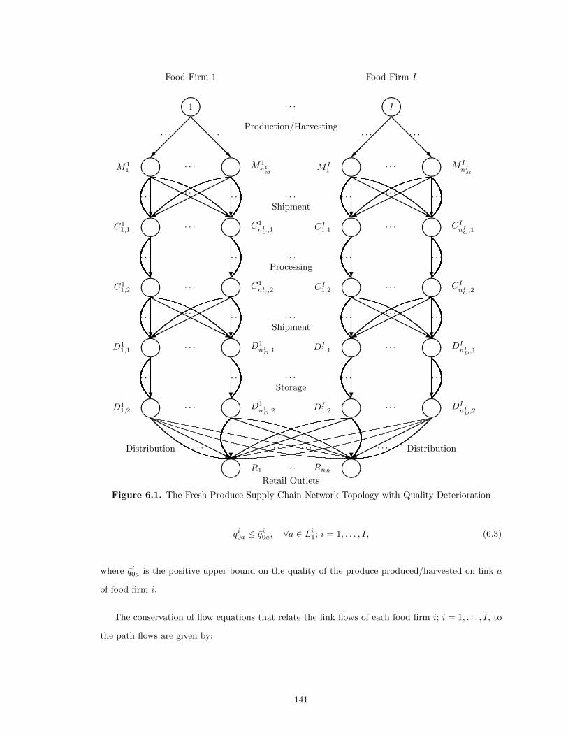
����R1 · · · RnR
Retail Outlets����
HHHHH
HHHHj
PPPPPPPPPPPPPPq?
��������������) ?
�����
�����· · · · · ·
· · · · · ·· · · · · ·· · · · · ·
D11,2 ���� · · · ����D1
n1D,2
DI1,2 ���� · · · ����DI
nID,2
DistributionDistribution
?
. . .
?
. . .
?
. . .
?
. . .· · ·
D11,1 ���� · · · ����D1
n1D,1
DI1,1 ���� · · · ����DI
nID,1
?
HHHHHH
HHHj?
������
���� ?
HHHHHH
HHHj?
������
����
· · · · · · · · · · · · · · · · · ·· · ·
C11,2 ���� · · · ����C1
n1C ,2
CI1,2 ���� · · · ����CInIC ,2
?
. . .
?
. . .
?
. . .
?
. . .· · ·
C11,1 ���� · · · ����C1
n1C ,1
Storage
Shipment
Processing
Shipment
CI1,1 ���� · · · ����CInIC ,1
?
HHHH
HHHHHj?
����
������ ?
HHHH
HHHHHj?
����
������
· · · · · · · · · · · · · · · · · ·· · ·
M11 ���� · · · ����M1
n1M
Production/Harvesting
M I1 ���� · · · ����M I
nIM
���
��
@@@@@R
��
���
@@@@@R
· · · · · · · · · · · ·
����1 ����I· · ·
Food Firm 1 Food Firm I
Figure 6.1. The Fresh Produce Supply Chain Network Topology with Quality Deterioration
qi0a ≤ qi0a, ∀a ∈ Li1; i = 1, . . . , I, (6.3)
where qi0a is the positive upper bound on the quality of the produce produced/harvested on link a
of food firm i.
The conservation of flow equations that relate the link flows of each food firm i; i = 1, . . . , I, to
the path flows are given by:
141
fl =∑p∈P
xpδlp, ∀l ∈ Li; i = 1, . . . , I, (6.4)
where fl denotes the flow on link l, δlp = 1, if link l is contained in path p, and 0, otherwise, and
P denotes the set of all paths. Therefore, since the supply chain networks of the firms do not share
any common links, the flow of a firm’s fresh produce product on a link is equal to the sum of that
product’s flows on paths that contain that link. We group the link flows into the vector f ∈ RnL+ ,
where nL denotes the number of links in L. All vectors in this chapter are column vectors.
In addition, since the link flows must satisfy capacity constraints, we have that:
fl ≤ ul, ∀l ∈ L, (6.5)
where ul denotes the positive upper bound on link l.
Also, observe that, in view of the conservation of flow equations (6.4), (6.5) can be rewritten in
terms of path flows as: ∑p∈P
xpδlp ≤ ul, ∀l ∈ L. (6.6)
In general, consumers, at the retail outlets, respond not only to the quantities available of the
product but also to their average quality, where the average quality of the product at retail outlet k,
associated with the fresh produce product of firm i, and denoted by qik, is given by the expression:
qik =
∑p∈P i
kqpxp∑
p∈P ikxp
, i = 1, . . . , I; k = R1, . . . , RnR, (6.7)
where recall that qp is fresh produce product specific with its value computed according to (5.8).
We group the average product quality of all firms into the vector q ∈ RI×nR+ . We exclude all food
firm / retail outlet pairs that do not conduct business with one another so that the denominator in
(6.7) is never equal to zero.
The demand for food firm i’s fresh food product at retail outlet k is denoted by dik and is equal
to the sum of all the fresh produce flows on paths joining (i, k), so that:
∑p∈P i
k
xp = dik, i = 1, . . . , I; k = R1, . . . , RnR. (6.8)
The demands for the fresh food products of all firms at all retail outlets are grouped into the vector
d ∈ RI×nR+ .
142
I now present the underlying functions in the competitive supply chain network model with
quality.
The demand price of food firm i’s product at retail outlet k is denoted by ρik and assume that
ρik = ρik(d, q), i = 1, . . . , I; k = R1, . . . , RnR. (6.9)
Note that the price of food firm i’s product at a particular retail outlet may depend not only
on the demands for and the average quality of its product, but also on the demands for and the
average quality of the other substitutable food products at all the retail outlets. These demand price
functions are assumed to be continuous, continuously differentiable, and monotone decreasing.
The cost of production/harvesting at firm i’s production site a depends, in general, on the initial
quality qi0a, and the product flow on the production/harvesting link, that is,
za = za(fa, qi0a), ∀a ∈ Li1; i = 1, . . . , I. (6.10)
Furthermore, the operational cost functions associated with the remaining links in the supply
chain network are defined as:
cb = cb(f), ∀b ∈ Li2; i = 1, . . . , I. (6.11)
The total operational cost on each such link is assumed to be convex and continuously differentiable
and the same holds for each production/harvesting cost function.
Let Xi denote the vector of path flows associated with firm i; i = 1, . . . , I, where Xi ≡ {{xp}|p ∈
P i}} ∈ RnPi
+ , P i ≡ ∪k=R1,...,RnRP ik, and nP i denotes the number of paths from firm origin node
i to the retail outlets. Then, X is the vector of all the food firms’ path flow strategies, that is,
X ≡ {{Xi}|i = 1, . . . , I}. Similarly, the vector of initial quality levels, associated with firm i;
i = 1, . . . , I, is denoted by qi0, where qi0 ≡ {{qi0a}|a ∈ Li1}} ∈ RnLi1
+ , where nLi1
is the number of
top-most links in firm i’s supply chain network. Finally, q0 is the vector of all initial quality levels
of the food firms; that is, q0 ≡ {{qi0}|i = 1, . . . , I}.
The utility of food firm i is its profit, which is the difference between its revenue and its total
costs, where the total costs are composed of the total costs on the production/harvesting links and
143
the total operational costs on the post-harvest links in its supply chain network. Hence, the utility
of firm i; i = 1, . . . , I, denoted by Ui, is expressed as:
Ui =
RnR∑k=R1
ρik(d, q)dik − (∑a∈Li
1
za(fa, qi0a) +
∑b∈Li
2
cb(f)). (6.12)
In view of (5.8), (6.5), and (6.8), (6.9) can be rewritten as:
ρik(x, q0) ≡ ρik(d, q), i = 1, . . . , I; k = R1, . . . , RnR. (6.13)
In lieu of the constraints (6.4) and (6.6), and the functional expressions (6.10), (6.11), and (6.13),
Ui(X, q0) ≡ Ui can be defined for all firms i; i = 1, . . . , I, with the I-dimensional vector U being the
vector of the profits of all the firms:
U = U(X, q0). (6.14)
In the competitive oligopolistic market framework, each firm selects its product path flows as well
as its initial quality levels at its production sites in a noncooperative manner, seeking to maximize
its own profit, until an equilibrium is achieved, according to the definition below:
• Definition 6.1: Supply Chain Network Nash Equilibrium with Fresh Produce Qual-
ity
A fresh produce path flow pattern and initial quality level (X∗, q∗0) ∈ K =∏Ii=1Ki constitutes
a supply chain network Nash Equilibrium with fresh produce quality if for each food firm i;
i = 1, . . . , I:
Ui(X∗i , X
∗−i, q
i∗0 , q
−i∗0 ) ≥ Ui(Xi, X
∗−i, q
i0, q−i∗0 ), ∀(Xi, q
i0) ∈ Ki, (6.15)
where X∗−i ≡ (X∗1 , . . . , X∗i−1, X
∗i+1, . . . , X
∗I ), q−i∗0 ≡ (q1∗0 , . . . , q
i−1∗0 , qi+1∗
0 , . . . , qI∗0 ) and
Ki ≡ {(Xi, qi0)|Xi ∈ R
nPi
+ , qi0 ∈ RnLi1
+ , (6.3) and (6.6) hold for l ∈ Li}.
In other words, an equilibrium is established if no food firm can unilaterally improve upon its
profit by altering its product flows and initial quality at production sites in its supply chain network,
given the product flows and initial quality decisions of the other firms.
144
Next, alternative variational inequality formulations of the Nash Equilibrium for the fresh pro-
duce supply chain network under oligopolistic competition satisfying Definition 6.1, in terms of path
flows and initial quality levels are derived (see Nash (1950, 1951)).
The λa; a ∈ L1 and γl; l ∈ L are the Lagrange multipliers associated with constraints (6.3) and
(6.6) (or (6.5)), respectively. We group these Lagrange multipliers into the nL1-dimensional vector
λ and the nL-dimensional vector γ, respectively.
• Theorem 6.1: Variational Inequality Formulation of the Governing Equilibrium
Conditions
Assume that, for each food firm i; i = 1, . . . , I, the profit function Ui(X, q0) is concave with
respect to the variables Xi and qi0, and is continuously differentiable. Then (X∗, q∗0) ∈ K is a
supply chain network Nash Equilibrium with fresh produce quality according to Definition 6.1
if and only if it satisfies the variational inequality:
−I∑i=1
〈∇XiUi(X∗, q∗0), Xi −X∗i 〉 −
I∑i=1
〈∇qi0Ui(X∗, q∗0), qi0 − qi∗0 〉 ≥ 0, ∀(X, q0) ∈ K, (6.16)
where 〈·, ·〉 denotes the inner product in the corresponding Euclidean space. Furthermore,
∇XiUi(X, q0) denotes the gradient of Ui(X, q0) with respect to Xi and ∇qi0Ui(X, q0) denotes
the gradient of Ui(X, q0) with respect to qi0. The solution of variational inequality (6.16), in
turn, is equivalent to the solution of the variational inequality: determine (x∗, q∗0 , λ∗, γ∗) ∈ K1
satisfying:
I∑i=1
RnR∑k=R1
∑p∈P i
k
∂Zi(x∗, qi∗0 )
∂xp+∂Ci(x∗)
∂xp+∑l∈Li
γ∗l δlp − ρik(x∗, q∗0)−RnR∑j=R1
∂ρij(x∗, q∗0)
∂xp
∑r∈P i
j
x∗r
×[xp − x∗p] +
I∑i=1
∑a∈Li
1
∂Zi(x∗, qi∗0 )
∂qi0a+ λ∗a −
RnR∑j=R1
∂ρij(x∗, q∗0)
∂qi0a
∑r∈P i
j
x∗r
× [qi0a − qi∗0a]
+
I∑i=1
∑a∈Li
1
[qi0a − qi∗0a
]×[λa−λ∗a]+
I∑i=1
∑l∈Li
[ul −
∑r∈P
x∗rδlr
]×[γl−γ∗l ] ≥ 0, ∀(x, q0, λ, γ) ∈ K1,
(6.17)
where K1 ≡ {(x, q0, λ, γ)|x ∈ RnP+ , q0 ∈ R
nL1+ , λ ∈ R
nL1+ , γ ∈ RnL
+ } and for each path p;
p ∈ P ik; i = 1, . . . , I; k = R1, . . . , RnR:
145
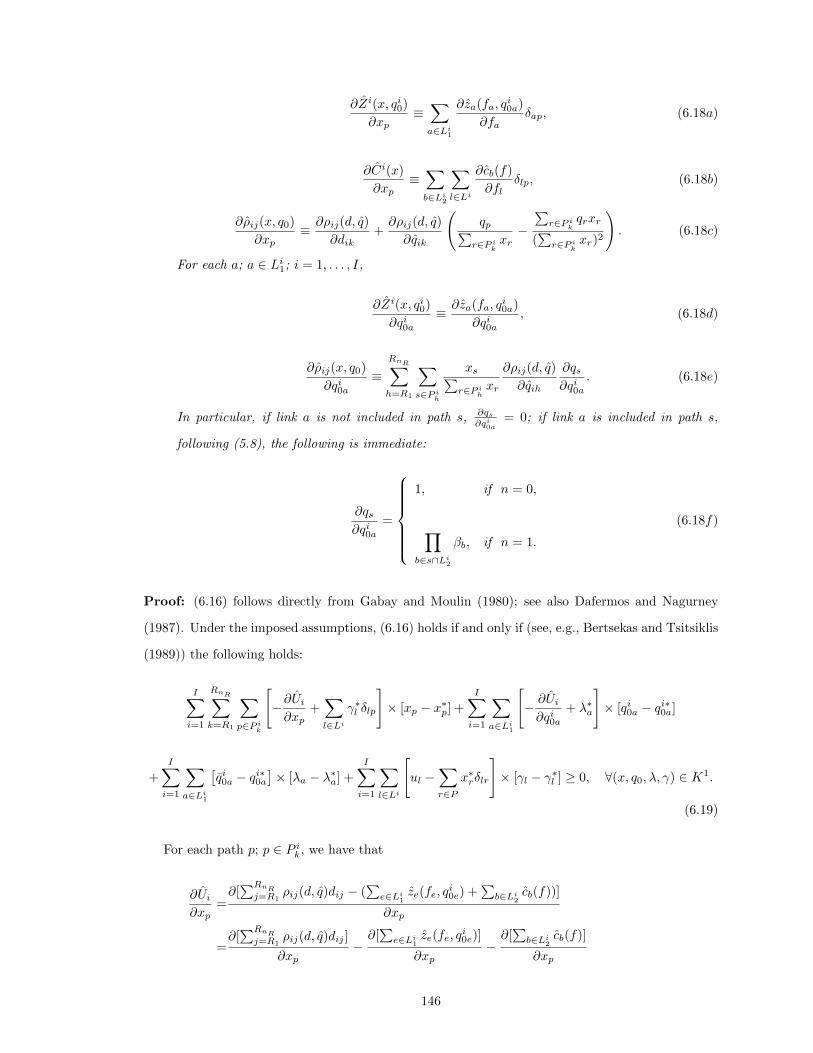
∂Zi(x, qi0)
∂xp≡∑a∈Li
1
∂za(fa, qi0a)
∂faδap, (6.18a)
∂Ci(x)
∂xp≡∑b∈Li
2
∑l∈Li
∂cb(f)
∂flδlp, (6.18b)
∂ρij(x, q0)
∂xp≡ ∂ρij(d, q)
∂dik+∂ρij(d, q)
∂qik
(qp∑
r∈P ikxr−∑r∈P i
kqrxr
(∑r∈P i
kxr)2
). (6.18c)
For each a; a ∈ Li1; i = 1, . . . , I,
∂Zi(x, qi0)
∂qi0a≡ ∂za(fa, q
i0a)
∂qi0a, (6.18d)
∂ρij(x, q0)
∂qi0a≡
RnR∑h=R1
∑s∈P i
h
xs∑r∈P i
hxr
∂ρij(d, q)
∂qih
∂qs∂qi0a
. (6.18e)
In particular, if link a is not included in path s, ∂qs∂qi0a
= 0; if link a is included in path s,
following (5.8), the following is immediate:
∂qs∂qi0a
=
1, if n = 0,
∏b∈s∩Li
2
βb, if n = 1.
(6.18f)
Proof: (6.16) follows directly from Gabay and Moulin (1980); see also Dafermos and Nagurney
(1987). Under the imposed assumptions, (6.16) holds if and only if (see, e.g., Bertsekas and Tsitsiklis
(1989)) the following holds:
I∑i=1
RnR∑k=R1
∑p∈P i
k
[−∂Ui∂xp
+∑l∈Li
γ∗l δlp
]× [xp − x∗p] +
I∑i=1
∑a∈Li
1
[− ∂Ui∂qi0a
+ λ∗a
]× [qi0a − qi∗0a]
+
I∑i=1
∑a∈Li
1
[qi0a − qi∗0a
]× [λa − λ∗a] +
I∑i=1
∑l∈Li
[ul −
∑r∈P
x∗rδlr
]× [γl − γ∗l ] ≥ 0, ∀(x, q0, λ, γ) ∈ K1.
(6.19)
For each path p; p ∈ P ik, we have that
∂Ui∂xp
=∂[∑RnR
j=R1ρij(d, q)dij − (
∑e∈Li
1ze(fe, q
i0e) +
∑b∈Li
2cb(f))]
∂xp
=∂[∑RnR
j=R1ρij(d, q)dij ]
∂xp−∂[∑e∈Li
1ze(fe, q
i0e)]
∂xp−∂[∑b∈Li
2cb(f)]
∂xp
146
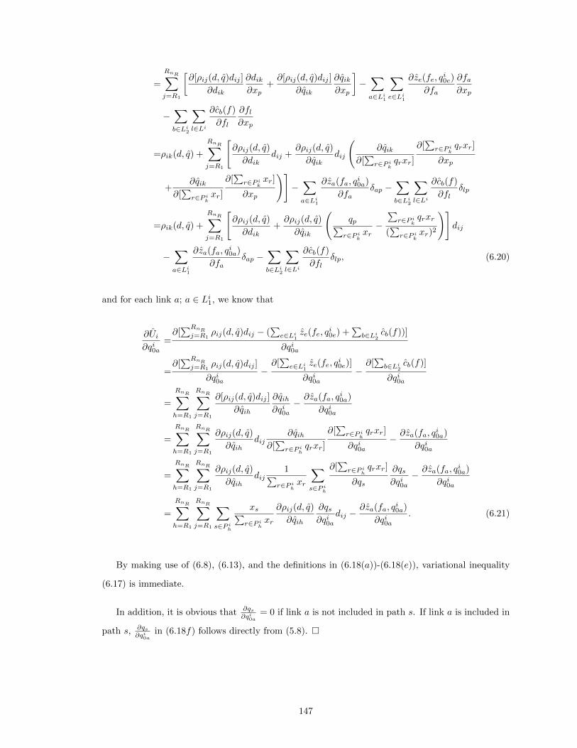
=
RnR∑j=R1
[∂[ρij(d, q)dij ]
∂dik
∂dik∂xp
+∂[ρij(d, q)dij ]
∂qik
∂qik∂xp
]−∑a∈Li
1
∑e∈Li
1
∂ze(fe, qi0e)
∂fa
∂fa∂xp
−∑b∈Li
2
∑l∈Li
∂cb(f)
∂fl
∂fl∂xp
=ρik(d, q) +
RnR∑j=R1
[∂ρij(d, q)
∂dikdij +
∂ρij(d, q)
∂qikdij
(∂qik
∂[∑r∈P i
kqrxr]
∂[∑r∈P i
kqrxr]
∂xp
+∂qik
∂[∑r∈P i
kxr]
∂[∑r∈P i
kxr]
∂xp
)]−∑a∈Li
1
∂za(fa, qi0a)
∂faδap −
∑b∈Li
2
∑l∈Li
∂cb(f)
∂flδlp
=ρik(d, q) +
RnR∑j=R1
[∂ρij(d, q)
∂dik+∂ρij(d, q)
∂qik
(qp∑
r∈P ikxr−∑r∈P i
kqrxr
(∑r∈P i
kxr)2
)]dij
−∑a∈Li
1
∂za(fa, qi0a)
∂faδap −
∑b∈Li
2
∑l∈Li
∂cb(f)
∂flδlp, (6.20)
and for each link a; a ∈ Li1, we know that
∂Ui∂qi0a
=∂[∑RnR
j=R1ρij(d, q)dij − (
∑e∈Li
1ze(fe, q
i0e) +
∑b∈Li
2cb(f))]
∂qi0a
=∂[∑RnR
j=R1ρij(d, q)dij ]
∂qi0a−∂[∑e∈Li
1ze(fe, q
i0e)]
∂qi0a−∂[∑b∈Li
2cb(f)]
∂qi0a
=
RnR∑h=R1
RnR∑j=R1
∂[ρij(d, q)dij ]
∂qih
∂qih∂qi0a
− ∂za(fa, qi0a)
∂qi0a
=
RnR∑h=R1
RnR∑j=R1
∂ρij(d, q)
∂qihdij
∂qih∂[∑r∈P i
hqrxr]
∂[∑r∈P i
hqrxr]
∂qi0a− ∂za(fa, q
i0a)
∂qi0a
=
RnR∑h=R1
RnR∑j=R1
∂ρij(d, q)
∂qihdij
1∑r∈P i
hxr
∑s∈P i
h
∂[∑r∈P i
hqrxr]
∂qs
∂qs∂qi0a
− ∂za(fa, qi0a)
∂qi0a
=
RnR∑h=R1
RnR∑j=R1
∑s∈P i
h
xs∑r∈P i
hxr
∂ρij(d, q)
∂qih
∂qs∂qi0a
dij −∂za(fa, q
i0a)
∂qi0a. (6.21)
By making use of (6.8), (6.13), and the definitions in (6.18(a))-(6.18(e)), variational inequality
(6.17) is immediate.
In addition, it is obvious that ∂qs∂qi0a
= 0 if link a is not included in path s. If link a is included in
path s, ∂qs∂qi0a
in (6.18f) follows directly from (5.8). �
147
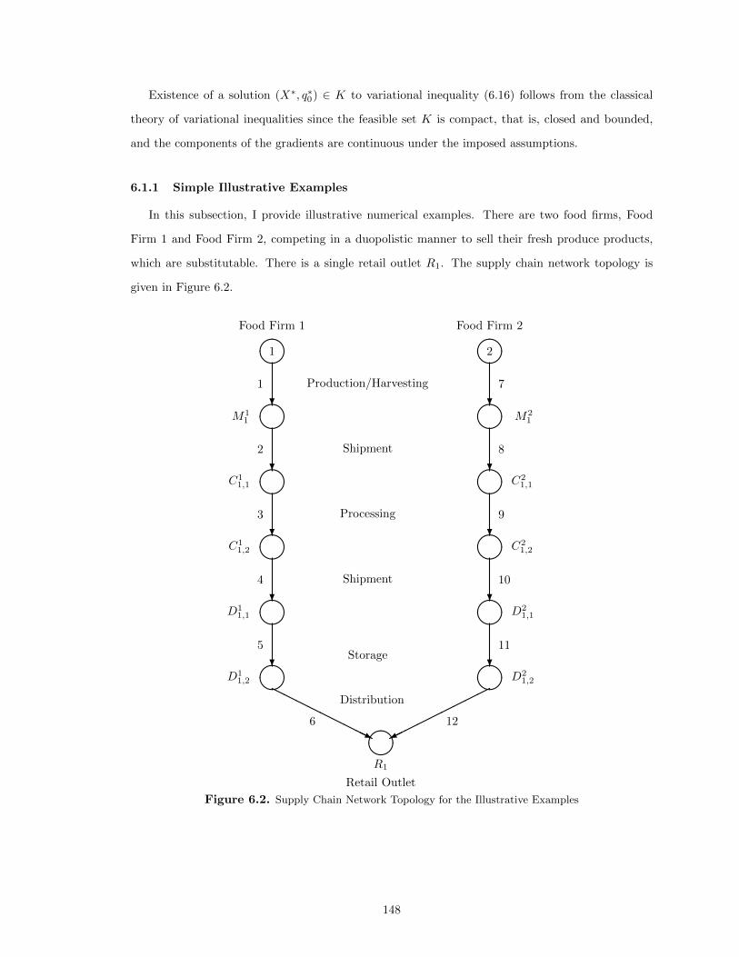
Existence of a solution (X∗, q∗0) ∈ K to variational inequality (6.16) follows from the classical
theory of variational inequalities since the feasible set K is compact, that is, closed and bounded,
and the components of the gradients are continuous under the imposed assumptions.
6.1.1 Simple Illustrative Examples
In this subsection, I provide illustrative numerical examples. There are two food firms, Food
Firm 1 and Food Firm 2, competing in a duopolistic manner to sell their fresh produce products,
which are substitutable. There is a single retail outlet R1. The supply chain network topology is
given in Figure 6.2.
����R1
Retail Outlet
HHHHHH
HHHj
������
����6 12
D11,2 ���� ����D2
1,2
? ?
5 11
D11,1 ���� D2
1,1����? ?
4 10
M11 M2
1
C11,1
C11,2 ����
C21,1
C21,2����? ?
3 9
���� ����? ?
2 8
���� ����? ?
1 7Production/Harvesting
Shipment
Processing
Shipment
Storage
Distribution
����1 ����2Food Firm 1 Food Firm 2
Figure 6.2. Supply Chain Network Topology for the Illustrative Examples
148
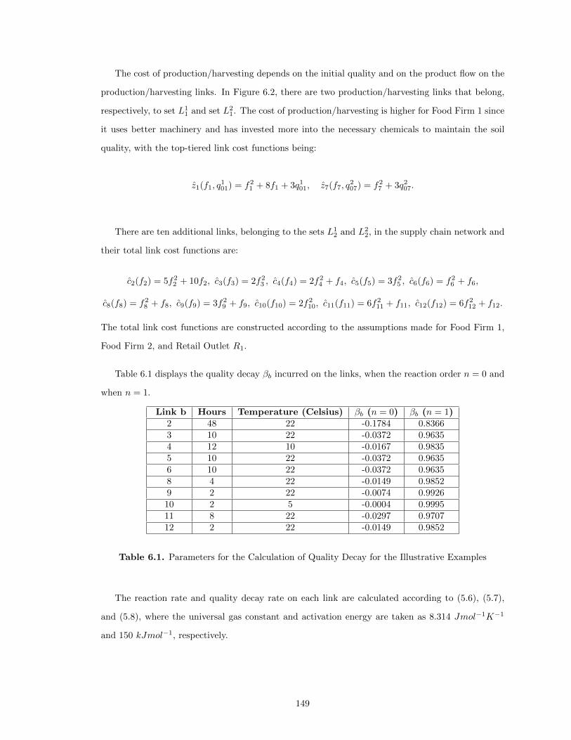
The cost of production/harvesting depends on the initial quality and on the product flow on the
production/harvesting links. In Figure 6.2, there are two production/harvesting links that belong,
respectively, to set L11 and set L2
1. The cost of production/harvesting is higher for Food Firm 1 since
it uses better machinery and has invested more into the necessary chemicals to maintain the soil
quality, with the top-tiered link cost functions being:
z1(f1, q101) = f21 + 8f1 + 3q101, z7(f7, q
207) = f27 + 3q207.
There are ten additional links, belonging to the sets L12 and L2
2, in the supply chain network and
their total link cost functions are:
c2(f2) = 5f22 + 10f2, c3(f3) = 2f23 , c4(f4) = 2f24 + f4, c5(f5) = 3f25 , c6(f6) = f26 + f6,
c8(f8) = f28 + f8, c9(f9) = 3f29 + f9, c10(f10) = 2f210, c11(f11) = 6f211 + f11, c12(f12) = 6f212 + f12.
The total link cost functions are constructed according to the assumptions made for Food Firm 1,
Food Firm 2, and Retail Outlet R1.
Table 6.1 displays the quality decay βb incurred on the links, when the reaction order n = 0 and
when n = 1.
Link b Hours Temperature (Celsius) βb (n = 0) βb (n = 1)2 48 22 -0.1784 0.83663 10 22 -0.0372 0.96354 12 10 -0.0167 0.98355 10 22 -0.0372 0.96356 10 22 -0.0372 0.96358 4 22 -0.0149 0.98529 2 22 -0.0074 0.992610 2 5 -0.0004 0.999511 8 22 -0.0297 0.970712 2 22 -0.0149 0.9852
Table 6.1. Parameters for the Calculation of Quality Decay for the Illustrative Examples
The reaction rate and quality decay rate on each link are calculated according to (5.6), (5.7),
and (5.8), where the universal gas constant and activation energy are taken as 8.314 Jmol−1K−1
and 150 kJmol−1, respectively.
149
The shipment time is longer for Food Firm 1 than for Food Firm 2 because of their respective
distances to their processing facilities, which can be seen from the time difference between link 2
and link 8.
There are two paths, p1 and p2, in this supply chain network, defined as: p1 = (1, 2, 3, 4, 5, 6)
and p2 = (7, 8, 9, 10, 11, 12). Since there exists one path for each food firm, it is known, because of
conservation of flow, that: d∗11 = x∗p1 and d∗21 = x∗p2 .
I now consider different quality decay functions and provide specific details in the examples
below.
6.1.2 Example 6.1a: Linear Quality Decay (Zero Order Kinetics)
As mentioned in Section 5.1, in a zero order quality decay function, the reaction order n = 0,
and the quality qp over a path p can be determined by the appropriate formula in (5.8), for n = 0.
The initial quality variables are q101 and q207.
The demand price functions are:
ρ11(x, q0) ≡ ρ11(d, q) = −2xp1 − xp2 +qp1xp1xp1
+ 100
and
ρ21(x, q0) ≡ ρ21(d, q) = −3xp2 − xp1 +qp2xp2xp2
+ 90,
with the path quality qp for the two paths constructed according to (5.8), for n = 0 for i = 1, 2,
given by:
qp1 = q101 + β2 + β3 + β4 + β5 + β6 = q101 − 0.3066,
qp2 = q207 + β8 + β9 + β10 + β11 + β12 = q207 − 0.0674.
The upper bounds (capacities) on the links are set to 200. Since the capacities on the links are
high, it is known that (cf. variational inequality (6.17)) the equilibrium Lagrange multipliers γ∗
associated with the links will be equal to 0. Similarly, for simplicity, and exposition purposes, the
initial quality bounds are set to 100, so that the corresponding equilibrium Lagrange multipliers λ∗,
based on the data, will also be 0.
150
Given the data, it is also reasonable to expect that x∗p1 > 0, x∗p2 > 0, q1∗01 > 0, and q2∗07 > 0.
Hence, in order to obtain the equilibrium path flows and the equilibrium initial quality levels that
satisfy variational inequality (6.17), the following expressions must be equal to 0:
∂Z1(x∗, q1∗01)
∂xp1+∂C1(x∗)
∂xp1− ρ11(x∗, q∗0)− ∂ρ11(x∗, q∗0)
∂xp1x∗p1 = 0, (6.22)
∂Z1(x∗, q1∗01)
∂q101− ∂ρ11(x∗, q∗0)
∂q101x∗p1 = 0, (6.23)
∂Z2(x∗, q2∗07)
∂xp2+∂C2(x∗)
∂xp2− ρ21(x∗, q∗0)− ∂ρ21(x∗, q∗0)
∂xp2x∗p2 = 0, (6.24)
∂Z2(x∗, q2∗07)
∂q207− ∂ρ21(x∗, q∗0)
∂q207x∗p2 = 0. (6.25)
Utilizing the functions for this example and (6.18a)− (6.18f), the following can be constructed:
∂C1(x∗)
∂xp1= 10x∗p1 + 10 + 4x∗p1 + 4x∗p1 + 1 + 6x∗p1 + 2x∗p1 + 1 = 26x∗p1 + 12,
∂Z1(x∗, q1∗01)
∂xp1= 2x∗p1 + 8,
−ρ11(x∗, q∗0) = 2x∗p1 + x∗p2 −(q1∗01 − 0.3066)x∗p1
x∗p1− 100 = 2x∗p1 + x∗p2 − q
1∗01 − 99.6934,
−∂ρ11(x∗, q∗0)
∂xp1x∗p1 = 2x∗p1 ,
∂Z1(x∗, q1∗01)
∂q101= 3,
−∂ρ11(x∗, q∗0)
∂q101x∗p1 = −x∗p1 .
Analogous expressions for path p2 are:
∂C2(x∗)
∂xp2= 2x∗p2 + 1 + 6x∗p2 + 1 + 4x∗p2 + 12x∗p2 + 1 + 12x∗p2 + 1 = 36x∗p2 + 4,
∂Z2(x∗, q2∗07)
∂xp2= 2x∗p2 ,
−ρ21(x∗, q∗0) = 3x∗p2 + x∗p1 −(q2∗07 − 0.0674)x∗p2
x∗p2− 90 = 3x∗p2 + x∗p1 − q
2∗07 − 89.9326,
−∂ρ21(x∗, q∗0)
∂xp2x∗p2 = 3x∗p2 ,
∂Z2(x∗, q2∗07)
∂q207= 3,
−∂ρ21(x∗, q∗0)
∂q207xp2 = −x∗p2 .
Grouping the terms above corresponding to each equation (6.22) – (6.25) obtain the following
system of equations are obtained:
151
32x∗p1 + x∗p2 − q1∗01 = 79.6934,
3− x∗p1 = 0,
x∗p1 + 44x∗p2 − q2∗07 = 85.9326,
3− x∗p2 = 0,
with solution:
x∗p1 = 3, x∗p2 = 3, q1∗01 = 19.3066, q2∗07 = 49.0674.
Hence, the path quality levels are: qp1 = 19 and qp2 = 49, the demand prices are: ρ11 = 110 and
ρ21 = 127, with Food Firm 1 enjoying a profit (in dollars) of U1(X∗, q∗0) = 87.0000 and Food Firm
2 a profit of U2(X∗, q∗0) = 51.0000.
Observe that Food Firm 1 has a higher profit than Food Firm 2, although its fresh produce is of
lower quality, both at its production site and at the retail outlet.
Next, I present an example with exponential quality decay.
6.1.3 Example 6.1b: Exponential Quality Decay (First Order Kinetics)
Example 6.1b is constructed from Example 6.1a and has the same data except that the product
now has an exponential quality decay with a reaction order n = 1. The quality levels of the paths
are constructed using the appropriate expression in (5.8) and the βb values in Table 6.1, for n = 1
for i = 1, 2, yielding:
qp1 = q101 × β2 × β3 × β4 × β5 × β6 = (q101)(0.7359),
qp2 = q207 × β8 × β9 × β10 × β11 × β12 = (q207)(0.9418).
I now proceed to solve the equations (6.22) – (6.25) for this example, with the following terms
for paths p1 and p2 presented for completeness and convenience:
−ρ11(x∗, q∗0) = 2x∗p1 + x∗p2 −(q1∗01)(0.7359)(x∗p1)
x∗p1− 100 = 2x∗p1 + x∗p2 − (q1∗01)(0.7359)− 100,
152
−∂ρ11(x∗, q∗0)
∂q101xp1 = −0.7359x∗p1 ,
−ρ21(x∗, q∗0) = 3x∗p2 + x∗p1 −(q2∗07)(0.9418)(x∗p2)
x∗p2− 90 = 3x∗p2 + x∗p1 − (q2∗07)(0.9418)− 90,
−∂ρ21(x∗, q∗0)
∂q207xp2 = −0.9418x∗p2 .
Grouping the terms above corresponding to each equation, I obtain the following system of
equations:
32x∗p1 + x∗p2 − 0.7359q1∗01 = 80,3− 0.7359x∗p1 = 0,
x∗p1 + 44x∗p2 − 0.9418q2∗07 = 86,
3− 0.9418x∗p2 = 0.
Straightforward calculations yield the following equilibrium path flows and equilibrium initial
quality levels:
x∗p1 = 4.0766, x∗p2 = 3.1854, q1∗01 = 72.8857, q2∗07 = 61.8329.
The path quality levels are, hence, qp1 = 53.6366 and qp2 = 58.2342.
Notice that, even though the initial quality of Food Firm 1’s fresh produce is higher, Food Firm
2 sells its fresh produce with a higher quality at the retail outlet.
By substituting the equilibrium path flows and the equilibrium initial qualities into the demand
price functions, I obtain the following equilibrium demand prices at the retail outlet for Food Firm
1 and Food Firm 2, respectively: ρ11 = 142.30 and ρ21 = 134.60. The price of Food Firm 2’s
fresh produce is higher than that of Food Firm 1’s. Furthermore, the profits of the food firms are
calculated, in dollars, as U1(X∗, q∗0) = 47.2497 and U2(X∗, q∗0) = 37.7258. Notice that, when the
quality decay becomes exponential, the profits of the food firms decrease significantly. It would
be reasonable to expect that food firms invest more to keep the initial quality high, hence, the end
quality would not get too low with a faster quality degradation. This causes the total cost to become
higher, therefore the the profits to decrease.
6.2. The Algorithm
Here I outline the computational procedure used to solve the examples in Section 3.3. Specifi-
cally, the variational inequality (6.26) is amenable to solution via the Euler method of Dupuis and
153
Nagurney (1993) which is described in Section 2.4. Below I present the closed form expression for
the path flows and initial quality levels.
6.2.1 Explicit Formulae for the Euler Method Applied to the Model
The closed form expressions for the fresh produce path flows at iteration τ + 1 are as follows.
For each path p ∈ P ik, ∀i, k, compute:
xτ+1p = max{0, xτp+ατ (ρik(xτ , qτ0 )+
RnR∑j=R1
∂ρij(xτ , qτ0 )
∂xp
∑r∈P i
j
xτr−∂Zi(xτ , qiτ0 )
∂xp−∂C
i(xτ )
∂xp−∑l∈Li
γτl δlp)}.
(6.27)
For each initial quality level a ∈ Li1, ∀i, in turn, compute:
qiτ+10a = max{0, qiτ0a + ατ (
RnR∑j=R1
∂ρij(xτ , qτ0 )
∂qi0a
∑r∈P i
j
xτr −∂Zi(xτ , qiτ0 )
∂qi0a− λτa)}. (6.28)
The Lagrange multiplier for each top-most link a ∈ Li1; i = 1, . . . , I, associated with the initial
quality bounds is computed as:
λτ+1a = max{0, λτa + ατ (qiτ0a − qi0a)}. (6.29)
Finally, the Lagrange multiplier for each link l ∈ Li; i = 1, . . . , I, associated with the link
capacities is computed according to:
γτ+1l = max{0, γτl + ατ (
∑r∈P
xτrδlr − ul)}. (6.30)
The expressions (6.27) through (6.30) may be interpreted as a discrete-time adjustment or taton-
nement process with the food firms updating at each discrete point in time their fresh produce path
flows, their initial quality levels as well as the Lagrange multipliers associated with the initial quality
levels at the production sites, and the Lagrange multipliers associated with the link capacities, until
an equilibrium is achieved. Observe that these computations can all be done simultaneously and,
hence, in parallel. Moreover, at each iteration, only the iterates from the preceding iteration (point
in time) are needed for these computations.
Next, I present larger numerical examples comprising a case study focusing on peaches.
154
6.3. A Case Study of Peaches
In this section, I focus on the peach market in the United States, specifically in Western Mas-
sachusetts. Peaches [Prunus persica (L.) Batsch] are very vital for fresh produce markets in the
United States and also all over the world. It is noted that, in 2015, the United States peach produc-
tion was 825,415 tons in volume, and 606 million dollars in worth (USDA NASS (2016), Zhao et al.
(2017)). For the case study, I selected two orchards from Western Massachusetts: Apex Orchards
and Cold Spring Orchard, located, respectively, in Shelburne, MA and Belchertown, MA. The supply
chain network topology for the peach case study is illustrated in Figure 6.3. It is assumed that the
Apex Orchards farm has two production sites, two processors, and two distribution centers. After
production/harvesting, Apex Orchards can ship its peaches to processors C11,1 or C1
2,1, with shipment
depicted via links 4, 5, 6, and 7 in Figure 3. Similarly, after processing, Apex Orchards can transfer
its peaches to D11,1 or D1
2,1, as shown in Figure 6.3 via links 12, 13, 14, and 15. Cold Spring Orchard
is smaller in size and, therefore, it only has only a single production site, one processor, and a single
distribution center. Both of the orchards sell their peaches to two retailers, Whole Foods, located in
Hadley, MA, and Formaggio Kitchen, located in Cambridge, MA. The mode of transportation for
both of the orchards is trucks.
According to Toralles et. al (2015), the color change attribute of peaches, in the form of brown-
ing, follows a first-order, that is, an exponential decay function. In Table 6.2, following (5.6), I
calculate the link quality degradation, βb, when the reaction order is n = 1, for the supply chain
network topology in Figure 6.3. The universal gas constant and activation energy are taken as 8.314
Jmol−1K−1 and 147.9 kJmol−1, respectively (Toralles et al. (2005)). The harvesting season for
peaches is usually mid-July to mid -September in Massachusetts, and the temperature reported in
Table 6.3, for the processing, shipment, and distribution links, is the average temperature of these
months. It is assumed that, since the Apex Orchards farm is located at a higher altitude, that the
average temperature of Apex’s operations is lower.
It is assumed that the shipment and distribution operations are made at an average temperature,
since the orchards do not have the necessary technology in their trucks to keep the temperature at
sufficient levels to deter quality degradation. Furthermore, according to Crisosto and Valero (2008)
the ideal storage temperature of peaches is between −1 C◦ and 1 C◦. In this case study, the Apex
Orchards owner is assumed to have the technology to keep the storage temperature at 1 C◦ and
Cold Spring Orchard is assumed to decrease the storage temperature only to 18 C◦. The product
155
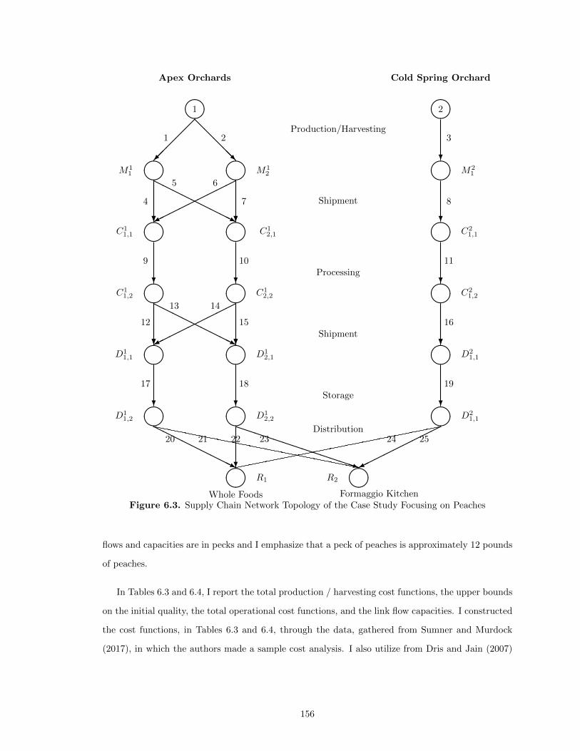
����R1 R2 ����Whole Foods Formaggio Kitchen
HHHHH
HHHHj
PPPPPPPPPPPPPPq?
�����
�����
20 21 22 23 24 25
D11,2 ���� ����D1
2,2 ����D21,1
? ? ?
17 18 19
D11,1 ���� ����D1
2,1 ����D21,1
C11,2 ���� ����C1
2,2 ����C21,2
? ? ?
9 10 11
C11,1 ���� ����C1
2,1 ����
? ? ?
C21,1
12
13 14
15 16
M11 ���� ����M1
2
Production/Harvesting
Shipment
Processing
Shipment
Storage
Distribution
����M21
? ? ?
4
5 6
7 8
��
���
@@@@@R
?
?
1 2 3
?
HHHHHH
HHHj?
������
����
?
HHHH
HHHHHj?
����
������
����1 ����2Apex Orchards Cold Spring Orchard
Figure 6.3. Supply Chain Network Topology of the Case Study Focusing on Peaches
flows and capacities are in pecks and I emphasize that a peck of peaches is approximately 12 pounds
of peaches.
In Tables 6.3 and 6.4, I report the total production / harvesting cost functions, the upper bounds
on the initial quality, the total operational cost functions, and the link flow capacities. I constructed
the cost functions, in Tables 6.3 and 6.4, through the data, gathered from Sumner and Murdock
(2017), in which the authors made a sample cost analysis. I also utilize from Dris and Jain (2007)
156
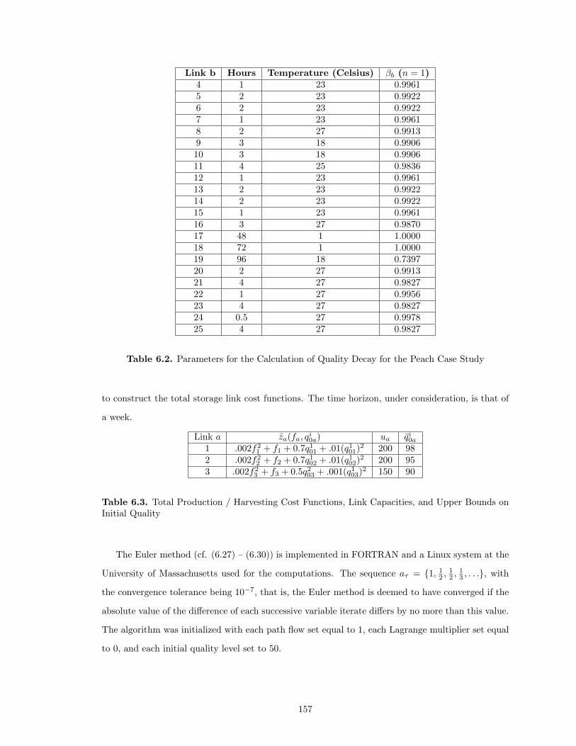
Link b Hours Temperature (Celsius) βb (n = 1)4 1 23 0.99615 2 23 0.99226 2 23 0.99227 1 23 0.99618 2 27 0.99139 3 18 0.990610 3 18 0.990611 4 25 0.983612 1 23 0.996113 2 23 0.992214 2 23 0.992215 1 23 0.996116 3 27 0.987017 48 1 1.000018 72 1 1.000019 96 18 0.739720 2 27 0.991321 4 27 0.982722 1 27 0.995623 4 27 0.982724 0.5 27 0.997825 4 27 0.9827
Table 6.2. Parameters for the Calculation of Quality Decay for the Peach Case Study
to construct the total storage link cost functions. The time horizon, under consideration, is that of
a week.
Link a za(fa, qi0a) ua qi0a
1 .002f21 + f1 + 0.7q101 + .01(q101)2 200 982 .002f22 + f2 + 0.7q102 + .01(q102)2 200 953 .002f23 + f3 + 0.5q203 + .001(q103)2 150 90
Table 6.3. Total Production / Harvesting Cost Functions, Link Capacities, and Upper Bounds onInitial Quality
The Euler method (cf. (6.27) – (6.30)) is implemented in FORTRAN and a Linux system at the
University of Massachusetts used for the computations. The sequence aτ = {1, 12 ,12 ,
13 , . . .}, with
the convergence tolerance being 10−7, that is, the Euler method is deemed to have converged if the
absolute value of the difference of each successive variable iterate differs by no more than this value.
The algorithm was initialized with each path flow set equal to 1, each Lagrange multiplier set equal
to 0, and each initial quality level set to 50.
157
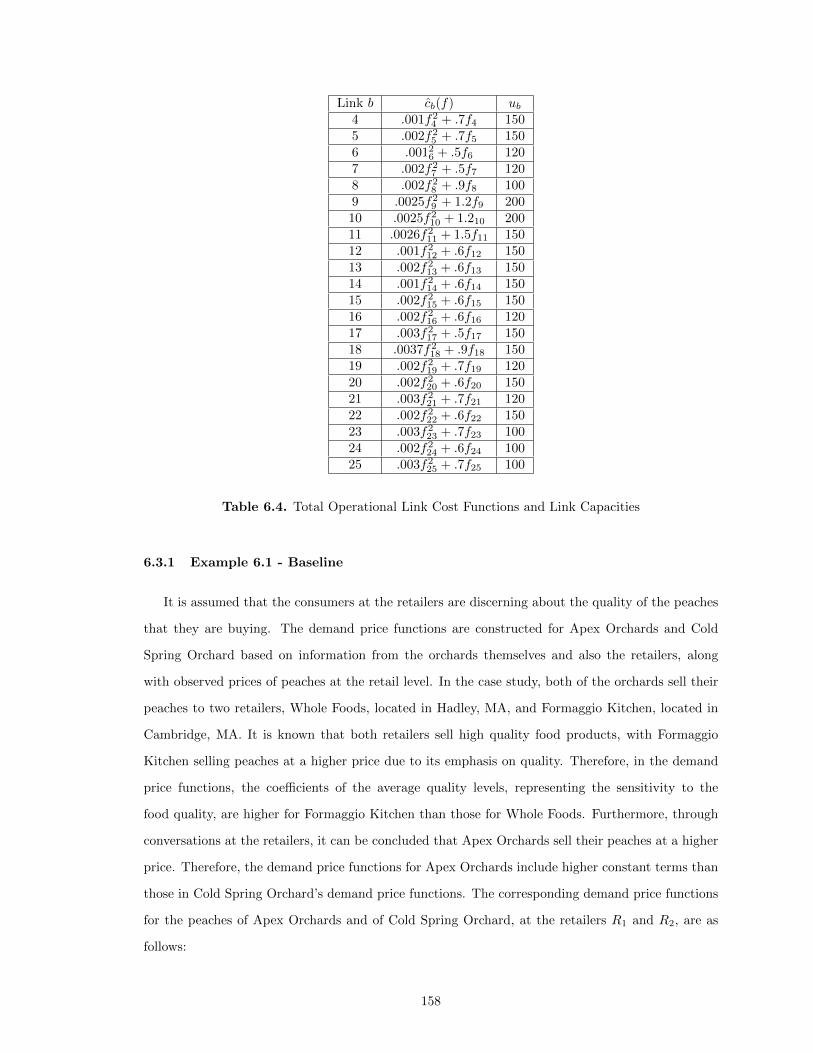
Link b cb(f) ub4 .001f24 + .7f4 1505 .002f25 + .7f5 1506 .00126 + .5f6 1207 .002f27 + .5f7 1208 .002f28 + .9f8 1009 .0025f29 + 1.2f9 20010 .0025f210 + 1.210 20011 .0026f211 + 1.5f11 15012 .001f212 + .6f12 15013 .002f213 + .6f13 15014 .001f214 + .6f14 15015 .002f215 + .6f15 15016 .002f216 + .6f16 12017 .003f217 + .5f17 15018 .0037f218 + .9f18 15019 .002f219 + .7f19 12020 .002f220 + .6f20 15021 .003f221 + .7f21 12022 .002f222 + .6f22 15023 .003f223 + .7f23 10024 .002f224 + .6f24 10025 .003f225 + .7f25 100
Table 6.4. Total Operational Link Cost Functions and Link Capacities
6.3.1 Example 6.1 - Baseline
It is assumed that the consumers at the retailers are discerning about the quality of the peaches
that they are buying. The demand price functions are constructed for Apex Orchards and Cold
Spring Orchard based on information from the orchards themselves and also the retailers, along
with observed prices of peaches at the retail level. In the case study, both of the orchards sell their
peaches to two retailers, Whole Foods, located in Hadley, MA, and Formaggio Kitchen, located in
Cambridge, MA. It is known that both retailers sell high quality food products, with Formaggio
Kitchen selling peaches at a higher price due to its emphasis on quality. Therefore, in the demand
price functions, the coefficients of the average quality levels, representing the sensitivity to the
food quality, are higher for Formaggio Kitchen than those for Whole Foods. Furthermore, through
conversations at the retailers, it can be concluded that Apex Orchards sell their peaches at a higher
price. Therefore, the demand price functions for Apex Orchards include higher constant terms than
those in Cold Spring Orchard’s demand price functions. The corresponding demand price functions
for the peaches of Apex Orchards and of Cold Spring Orchard, at the retailers R1 and R2, are as
follows:
158
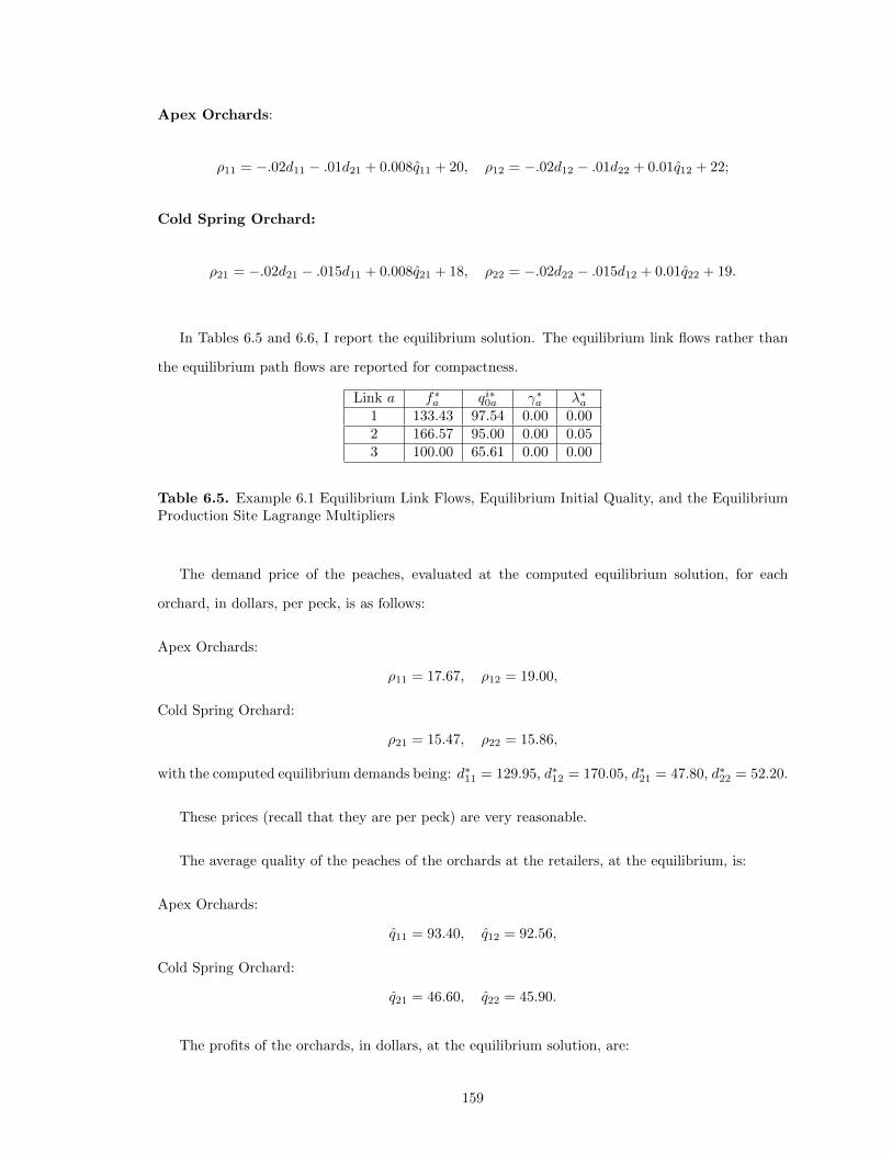
Apex Orchards:
ρ11 = −.02d11 − .01d21 + 0.008q11 + 20, ρ12 = −.02d12 − .01d22 + 0.01q12 + 22;
Cold Spring Orchard:
ρ21 = −.02d21 − .015d11 + 0.008q21 + 18, ρ22 = −.02d22 − .015d12 + 0.01q22 + 19.
In Tables 6.5 and 6.6, I report the equilibrium solution. The equilibrium link flows rather than
the equilibrium path flows are reported for compactness.
Link a f∗a qi∗0a γ∗a λ∗a1 133.43 97.54 0.00 0.002 166.57 95.00 0.00 0.053 100.00 65.61 0.00 0.00
Table 6.5. Example 6.1 Equilibrium Link Flows, Equilibrium Initial Quality, and the EquilibriumProduction Site Lagrange Multipliers
The demand price of the peaches, evaluated at the computed equilibrium solution, for each
orchard, in dollars, per peck, is as follows:
Apex Orchards:
ρ11 = 17.67, ρ12 = 19.00,
Cold Spring Orchard:
ρ21 = 15.47, ρ22 = 15.86,
with the computed equilibrium demands being: d∗11 = 129.95, d∗12 = 170.05, d∗21 = 47.80, d∗22 = 52.20.
These prices (recall that they are per peck) are very reasonable.
The average quality of the peaches of the orchards at the retailers, at the equilibrium, is:
Apex Orchards:
q11 = 93.40, q12 = 92.56,
Cold Spring Orchard:
q21 = 46.60, q22 = 45.90.
The profits of the orchards, in dollars, at the equilibrium solution, are:
159
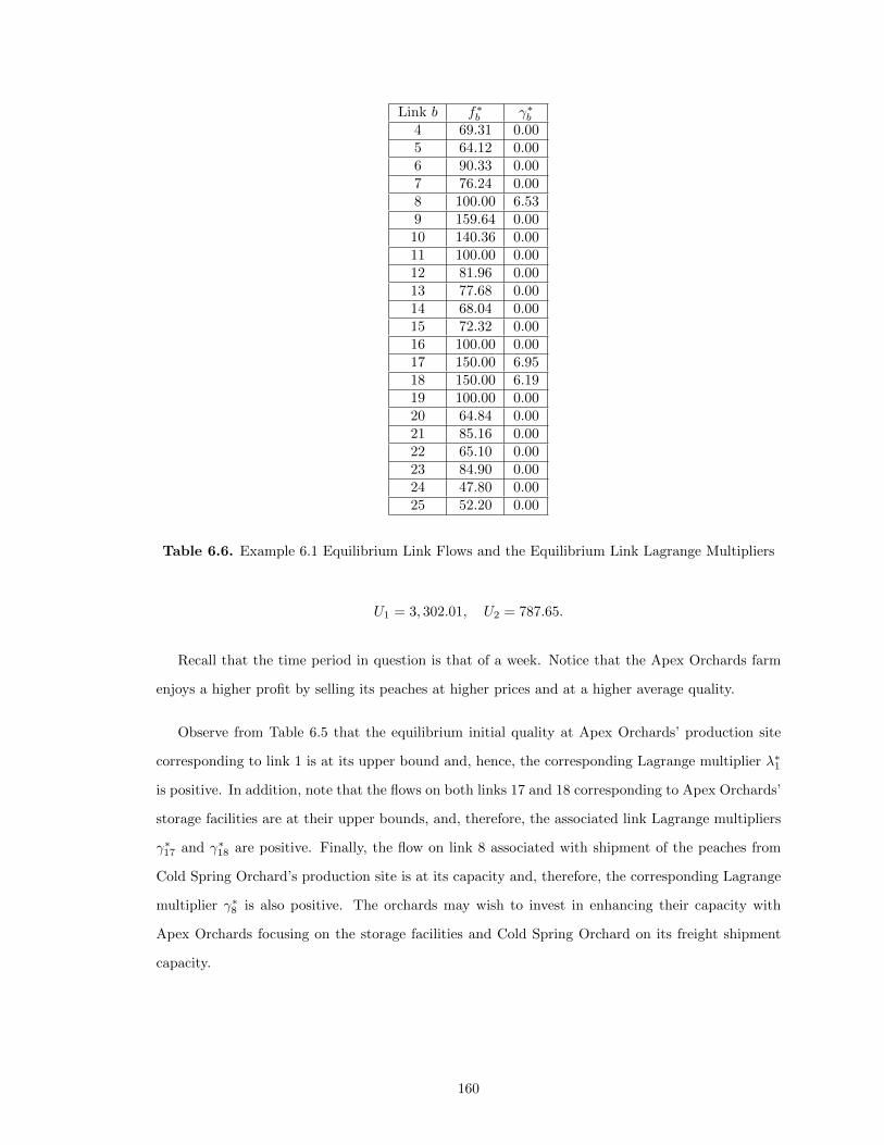
Link b f∗b γ∗b4 69.31 0.005 64.12 0.006 90.33 0.007 76.24 0.008 100.00 6.539 159.64 0.0010 140.36 0.0011 100.00 0.0012 81.96 0.0013 77.68 0.0014 68.04 0.0015 72.32 0.0016 100.00 0.0017 150.00 6.9518 150.00 6.1919 100.00 0.0020 64.84 0.0021 85.16 0.0022 65.10 0.0023 84.90 0.0024 47.80 0.0025 52.20 0.00
Table 6.6. Example 6.1 Equilibrium Link Flows and the Equilibrium Link Lagrange Multipliers
U1 = 3, 302.01, U2 = 787.65.
Recall that the time period in question is that of a week. Notice that the Apex Orchards farm
enjoys a higher profit by selling its peaches at higher prices and at a higher average quality.
Observe from Table 6.5 that the equilibrium initial quality at Apex Orchards’ production site
corresponding to link 1 is at its upper bound and, hence, the corresponding Lagrange multiplier λ∗1
is positive. In addition, note that the flows on both links 17 and 18 corresponding to Apex Orchards’
storage facilities are at their upper bounds, and, therefore, the associated link Lagrange multipliers
γ∗17 and γ∗18 are positive. Finally, the flow on link 8 associated with shipment of the peaches from
Cold Spring Orchard’s production site is at its capacity and, therefore, the corresponding Lagrange
multiplier γ∗8 is also positive. The orchards may wish to invest in enhancing their capacity with
Apex Orchards focusing on the storage facilities and Cold Spring Orchard on its freight shipment
capacity.
160
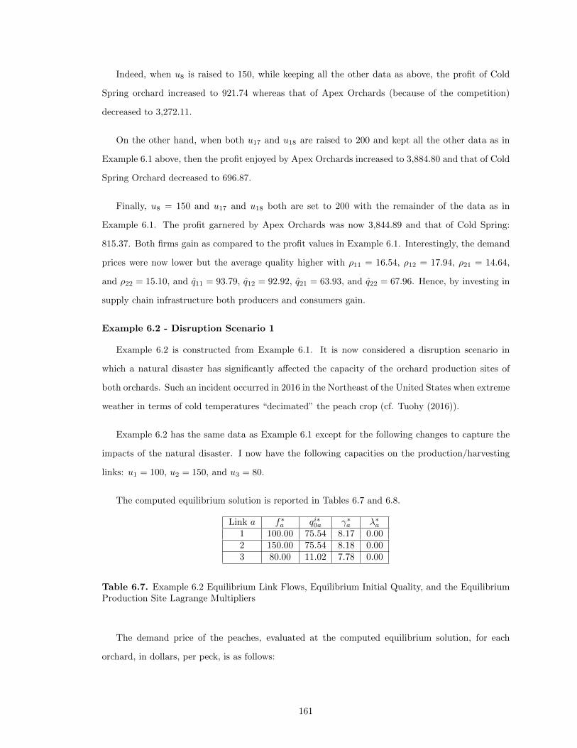
Indeed, when u8 is raised to 150, while keeping all the other data as above, the profit of Cold
Spring orchard increased to 921.74 whereas that of Apex Orchards (because of the competition)
decreased to 3,272.11.
On the other hand, when both u17 and u18 are raised to 200 and kept all the other data as in
Example 6.1 above, then the profit enjoyed by Apex Orchards increased to 3,884.80 and that of Cold
Spring Orchard decreased to 696.87.
Finally, u8 = 150 and u17 and u18 both are set to 200 with the remainder of the data as in
Example 6.1. The profit garnered by Apex Orchards was now 3,844.89 and that of Cold Spring:
815.37. Both firms gain as compared to the profit values in Example 6.1. Interestingly, the demand
prices were now lower but the average quality higher with ρ11 = 16.54, ρ12 = 17.94, ρ21 = 14.64,
and ρ22 = 15.10, and q11 = 93.79, q12 = 92.92, q21 = 63.93, and q22 = 67.96. Hence, by investing in
supply chain infrastructure both producers and consumers gain.
Example 6.2 - Disruption Scenario 1
Example 6.2 is constructed from Example 6.1. It is now considered a disruption scenario in
which a natural disaster has significantly affected the capacity of the orchard production sites of
both orchards. Such an incident occurred in 2016 in the Northeast of the United States when extreme
weather in terms of cold temperatures “decimated” the peach crop (cf. Tuohy (2016)).
Example 6.2 has the same data as Example 6.1 except for the following changes to capture the
impacts of the natural disaster. I now have the following capacities on the production/harvesting
links: u1 = 100, u2 = 150, and u3 = 80.
The computed equilibrium solution is reported in Tables 6.7 and 6.8.
Link a f∗a qi∗0a γ∗a λ∗a1 100.00 75.54 8.17 0.002 150.00 75.54 8.18 0.003 80.00 11.02 7.78 0.00
Table 6.7. Example 6.2 Equilibrium Link Flows, Equilibrium Initial Quality, and the EquilibriumProduction Site Lagrange Multipliers
The demand price of the peaches, evaluated at the computed equilibrium solution, for each
orchard, in dollars, per peck, is as follows:
161
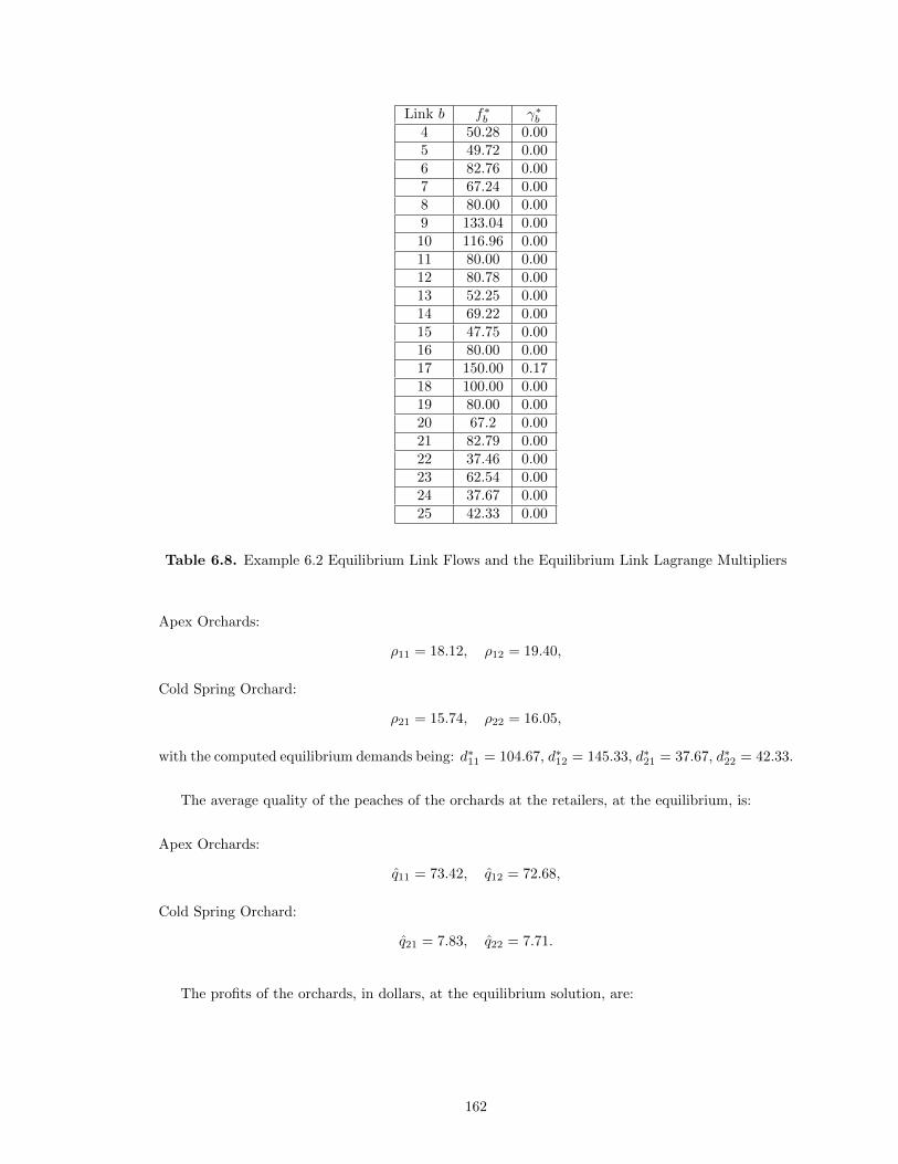
Link b f∗b γ∗b4 50.28 0.005 49.72 0.006 82.76 0.007 67.24 0.008 80.00 0.009 133.04 0.0010 116.96 0.0011 80.00 0.0012 80.78 0.0013 52.25 0.0014 69.22 0.0015 47.75 0.0016 80.00 0.0017 150.00 0.1718 100.00 0.0019 80.00 0.0020 67.2 0.0021 82.79 0.0022 37.46 0.0023 62.54 0.0024 37.67 0.0025 42.33 0.00
Table 6.8. Example 6.2 Equilibrium Link Flows and the Equilibrium Link Lagrange Multipliers
Apex Orchards:
ρ11 = 18.12, ρ12 = 19.40,
Cold Spring Orchard:
ρ21 = 15.74, ρ22 = 16.05,
with the computed equilibrium demands being: d∗11 = 104.67, d∗12 = 145.33, d∗21 = 37.67, d∗22 = 42.33.
The average quality of the peaches of the orchards at the retailers, at the equilibrium, is:
Apex Orchards:
q11 = 73.42, q12 = 72.68,
Cold Spring Orchard:
q21 = 7.83, q22 = 7.71.
The profits of the orchards, in dollars, at the equilibrium solution, are:
162
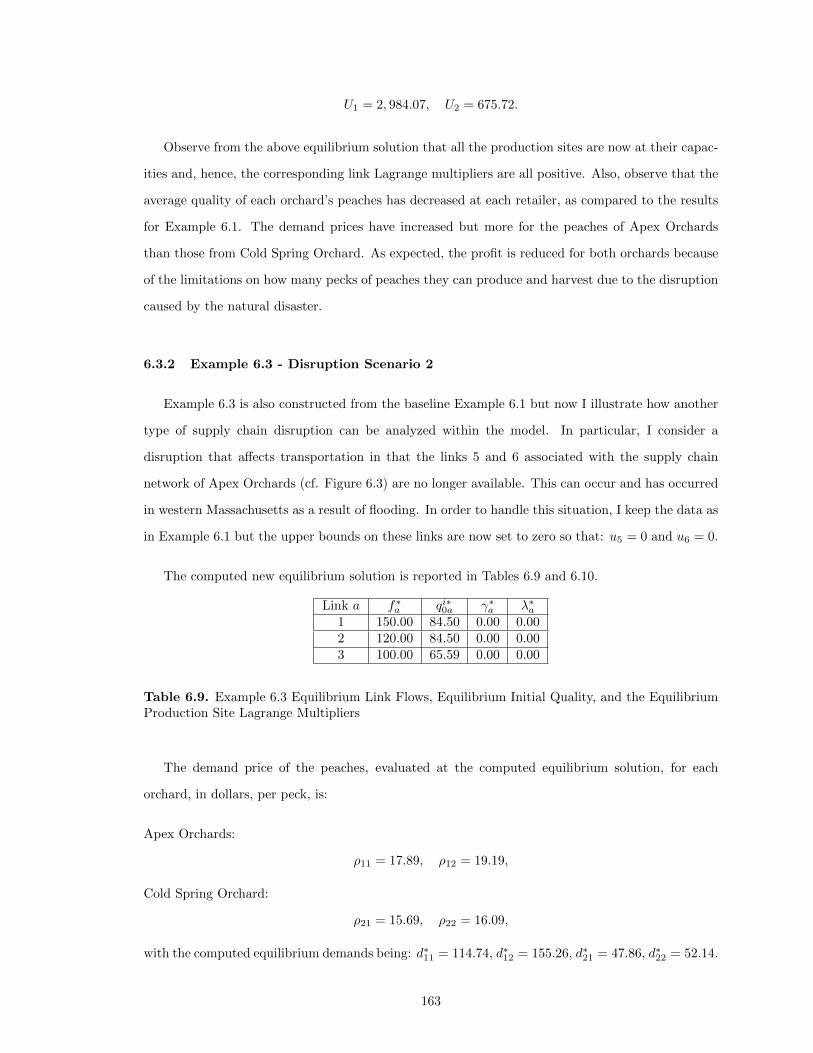
U1 = 2, 984.07, U2 = 675.72.
Observe from the above equilibrium solution that all the production sites are now at their capac-
ities and, hence, the corresponding link Lagrange multipliers are all positive. Also, observe that the
average quality of each orchard’s peaches has decreased at each retailer, as compared to the results
for Example 6.1. The demand prices have increased but more for the peaches of Apex Orchards
than those from Cold Spring Orchard. As expected, the profit is reduced for both orchards because
of the limitations on how many pecks of peaches they can produce and harvest due to the disruption
caused by the natural disaster.
6.3.2 Example 6.3 - Disruption Scenario 2
Example 6.3 is also constructed from the baseline Example 6.1 but now I illustrate how another
type of supply chain disruption can be analyzed within the model. In particular, I consider a
disruption that affects transportation in that the links 5 and 6 associated with the supply chain
network of Apex Orchards (cf. Figure 6.3) are no longer available. This can occur and has occurred
in western Massachusetts as a result of flooding. In order to handle this situation, I keep the data as
in Example 6.1 but the upper bounds on these links are now set to zero so that: u5 = 0 and u6 = 0.
The computed new equilibrium solution is reported in Tables 6.9 and 6.10.
Link a f∗a qi∗0a γ∗a λ∗a1 150.00 84.50 0.00 0.002 120.00 84.50 0.00 0.003 100.00 65.59 0.00 0.00
Table 6.9. Example 6.3 Equilibrium Link Flows, Equilibrium Initial Quality, and the EquilibriumProduction Site Lagrange Multipliers
The demand price of the peaches, evaluated at the computed equilibrium solution, for each
orchard, in dollars, per peck, is:
Apex Orchards:
ρ11 = 17.89, ρ12 = 19.19,
Cold Spring Orchard:
ρ21 = 15.69, ρ22 = 16.09,
with the computed equilibrium demands being: d∗11 = 114.74, d∗12 = 155.26, d∗21 = 47.86, d∗22 = 52.14.
163
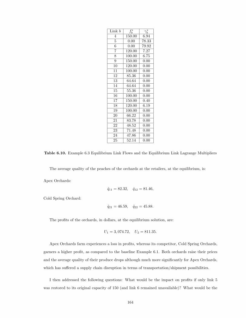
Link b f∗b γ∗b4 150.00 6.945 0.00 78.336 0.00 79.927 120.00 7.278 100.00 6.759 150.00 0.0010 120.00 0.0011 100.00 0.0012 85.36 0.0013 64.64 0.0014 64.64 0.0015 55.36 0.0016 100.00 0.0017 150.00 0.4018 120.00 6.1919 100.00 0.0020 66.22 0.0021 83.78 0.0022 48.52 0.0023 71.48 0.0024 47.86 0.0025 52.14 0.00
Table 6.10. Example 6.3 Equilibrium Link Flows and the Equilibrium Link Lagrange Multipliers
The average quality of the peaches of the orchards at the retailers, at the equilibrium, is:
Apex Orchards:
q11 = 82.32, q12 = 81.46,
Cold Spring Orchard:
q21 = 46.59, q22 = 45.88.
The profits of the orchards, in dollars, at the equilibrium solution, are:
U1 = 3, 074.72, U2 = 811.35.
Apex Orchards farm experiences a loss in profits, whereas its competitor, Cold Spring Orchards,
garners a higher profit, as compared to the baseline Example 6.1. Both orchards raise their prices
and the average quality of their produce drops although much more significantly for Apex Orchards,
which has suffered a supply chain disruption in terms of transportation/shipment possibilities.
I then addressed the following questions: What would be the impact on profits if only link 5
was restored to its original capacity of 150 (and link 6 remained unavailable)? What would be the
164
impact on profits if only link 6 was restored to its original capacity of 120 (and link 5 remained
unavailable)? I found the following: The profit of Apex Orchards was 3,272.78 with link 5 restored
only and that of Cold Spring Orchard was: 787.64. On the other hand, if link 6 was restored only,
then Apex Orchards garnered 3,283.32 in profit and Cold Spring Orchard 787.67 in profit. Hence,
given the choice, Apex Orchards should advocate for restoration of link 6 versus link 5 if only one
link restoration is feasible.
6.4. Summary and Conclusions
In this chapter, I constructed a general framework for the modeling, analysis, and computation
of solutions to competitive fresh produce supply chain networks in which food firm owners seek to
maximize their profits while determining both the initial quality of the fresh produce with associated
costs as well as the fresh produce flows along pathways of their supply chain network through the
various activities of harvesting, processing, storage, and distribution. In this framework, I utilize
explicit formulae associated with quality deterioration on the supply chain network links which are
a function of physical characteristics, including temperature and time. The prices at the retailers
are a function not only of the demand for the produce but also of the average quality level of the
produce at the retailers.
I provide the governing Nash Equilibrium conditions and the alternative variational inequality
formulations. The algorithm is presented, which shows a discrete-time adjustment process, and
which yields closed form expressions at each iteration for the product path flows, the initial quality
levels, as well as the Lagrange multipliers associated with the link capacities and the initial quality
upper bounds. I present examples to illustrate the mathematical framework and provide a case
study on peaches, consisting of numerical examples under status quo and disruption scenarios.
165
CHAPTER 7
CONCLUSIONS AND FUTURE RESEARCH
7.1. Conclusions
In this dissertation, my goal was to study the challenging issues on supply chains in the food
industry. I focused on two main issues: impacts of trade and policy instruments, and the fresh
produce quality deterioration. The mathematical models in this dissertation were based on the
economics of competitive supply chain networks. The results that I observed through simulated case
studies with various scenarios can inform policy makers.
In this dissertation, I contributed to the literature on variational inequalities, game theory, and
supply chain network equilibrium modeling. In Chapter 3 of this dissertation, I provided a unified
variational inequality framework for the modeling, analysis, and computation of solutions to a general
spatial network equilibrium problem in the presence of tariff-rate quotas. The supply chain network
equilibrium model considers multiple countries and regions in each country. In Chapter 4, I extended
the mathematical model constructed in Chapter 3 by incorporating quality as a strategic variable.
In this chapter, I also studied an imperfectly competitive model in the form of an oligopoly. In
Chapter 5, I presented a modeling and algorithmic framework for competitive farmers’ markets by
integrating fresh produce quality deterioration explicitly by chemical formulae depending on time
and temperature. I extended this model in Chapter 6 by including initial quality of the food product
as a strategic variable.
7.2. Future Research
I intend to construct a global food supply chain equilibrium model through the integration of
trade instruments and exchange rates while capturing the quality deterioration of perishable food
products. I will specifically focus on banana supply chain networks as an example of global food
chain networks. My goal in the future is to connect the previous chapters of this dissertation,
focusing both on the modeling of trade instruments and fresh produce quality deterioration, in a
single unifying mathematical modeling framework.
166
Bananas, the most consumed fruit in the United States, greater than the amount of apples
and oranges combined (Koeppel (2008)), are excellent sources for gaining necessary vitamins, and
minerals such as potassium, magnesium, sodium, and iron (UN (2016)). Bananas are also relatively
cheap and are available in many parts of the world. These advantages make bananas one of most
frequently bought fruit, accounting for about 14.1 million metric tons export volume in 2006 (Liu
(2009)).
As mentioned in Chapter 1, global food supply chain networks are very unique, since the products
have a perishable nature. Banana supply chain networks are very similar to other fresh produce
supply chain networks, in terms of their perishable nature, but they are also very distinctive with
their high consumption levels. This creates a highly competitive environment, coupled with high
quality expectations, and the logistical challenges emerging from the long distances.
The two biggest banana importers in the world are the US and the European Union, whereas the
biggest exporter of bananas is Ecuador. The other major export countries of bananas are: Costa
Rica, the Dominican Republic, Colombia, and Peru (Liu (2009)). Hence, in the banana supply chain
network that I plan on formulating, the first tier will consist of farms located in countries such as:
the Dominican Republic, Ecuador, Peru, Colombia, Costa Rica, and Honduras. Furthermore, the
demand points will be the supermarkets in the countries such as: the United States, the United
Kingdom, Canada, Germany, or France.
Trade instruments in the form of tariff rate quotas are being used frequently in the global banana
trade. In the 2000s, the European Union and Latin American banana exporters were engaged in a
dispute over banana trade, in which they reached an agreement resulting in the decrease of tariffs
gradually, beginning in 2011. However, according to Vega (2011), Ecuador still faces high import
duties while entering the European markets. As I also mention in Section 1.4.5, exchange rates are
also affecting the fresh produce trade negatively, resulting from the currency fluctuations in Latin
America.
It would be of great value to study the effects of trade instruments, and quality deterioration in
global banana trade. I will also attempt to integrate exchange rates into the modeling of a banana
supply chain network model. I also wish to include another tier of decision makers, in the form of
wholesalers, and to investigate the impacts on quality deterioration. The results obtained from this
research can inform food firms, policy makers, and regulators.
167
BIBLIOGRAPHY
Aamir, M., Ovissipour, M., Sablani, S.S., Rasco, B., 2013. Predicting the quality of pasteurizedvegetables using kinetic models: a review. International Journal of Food Science, Article ID 271271.
Abbott, J.A., 1999. Quality measurement of fruits and vegetables. Postharvest Biology and Tech-nology, 15(3), 207-225.
Ahumada, O., Villalobos, J.R., 2007. Application of planning models in the agri-food supply chain:A review. European Journal of Operational Research, 196(1), 1-20.
Ahumada, O., Villalobos, J.R., 2011. A tactical model for planning the production and distributionof fresh produce. Annals of Operations Research, 190(1), 339-358.
Aiello, G., La, Scalia G., Micale, R., 2012. Simulation analysis of cold chain performance based ontime-temperature data. Production Planning & Control, 23(6), 468-476.
Akkerman, R., Farahani, P., Grunow, M., 2010. Quality, safety and sustainability in food distribu-tion: A review of quantitative operations management approaches and challenges. OR Spectrum,32(4), 863-904.
Alliance, F.C.W., 2016. No Piece of the Pie: US Food Workers. Solidarity Research Cooperative.
Amorum, P., Costa A.M., Almada-Lobo, B., 2014. Influence of consumer purchasing behaviour onthe production planning of perishable food. OR Spectrum, 36(3), 669-692.
Appelbaum, B., 2018. Their soybeans piling up, farmers’ hope trade war ends before beans rot. TheNew York Times, November 5.
Aregu, R., 2014. Market and Price Decision Enhancement Services for Farmers in Uganda. DoctoralDissertation, University of Groningen, Groningen, The Netherlands.
Arrhenius, S., 1889. Uber die reaktionsgeschwindigkeit bei der inversion von rohrzucker durch suren.Zeitschrift Fur Physikalische Chemie, 4, 226-248.
Arrow, K.J., Debreu, G., 1954. Existence of an equilibrium for a competitive economy. Economet-rica, 22, 265-290.
Asebo, K., Moxnes J. A., Lieblein, G., Svennerud, M., Francis, C., 2007. Farmer and consumerattitudes at farmers’ markets in Norway. Journal of Sustainable Agriculture, 30(4), 67-93.
Ash, M.S., Livezey, J., Dohlman, E.N., 2006. Soybean backgrounder. US Department of Agriculture,Economic Research Service, Washington DC.
Asmuth, R., Eaves, C.B., Peterson, E.L., 1979. Computing economic equilibria on affine networkswith Lemke’s algorithm. Mathematics of Operations Research, 4(3), 209-214.
168
Aw, B.Y., Roberts, M.J., 1986. Measuring quality in quota-constrained import markets: The caseof U.S. footwear. Journal of International Economics, 21(1/2), 45-60.
Babiak, L., 2013. Exploring Local Food System Practices and Perceptions: Insights from Florida’sSNAP Authorized Farmers’ Markets. Master of Science Thesis. Department of Geography, Envi-ronment, and Planning, College of Arts and Sciences, University of South Florida, Tampa, Florida.
Baiocchi, C., Capelo, A., 1984. Variational and Quasi-variational Inequalities J. Wiley and Sons,New York.
Barrett, D.M., Beaulieu, J.C., Shewfelt, R., 2010. Color, flavor, texture, and nutritional qualityof fresh-cut fruits and vegetables: desirable levels, instrumental and sensory measurement, and theeffects of processing. Critical Reviews in Food Science and Nutrition, 50(5), 369-389.
Bensoussan, A., Lions, J.L., 1978. Applications des Inequations Variationelles en Control et enStochastiques. Dunod, Paris, France.
Berkett, L.P., 1994. Management Guide for Low-Input Sustainable Apple Production. DIANEPublishing, May 1.
Bertsekas, D.P., Tsitsiklis, J.N., 1989. Parallel and Distributed Computation. Prentice-Hall, Engle-wood Cliffs, New Jersey.
Besik, D., Nagurney, A., 2017. Quality in fresh produce supply chains with application to farmers’markets. Socio-Economic Planning Sciences, 60, 62-76.
Bhagwati, J., 1965. On the equivalence of tariffs and quotas. In: Trade, Growth and the Balanceof Payments: Essays in Honor of G. Haberler, Baldwin, R.E., Bhagwati, J., Caves, R.E., Johnson,H.G. (Editors). Rand McNally, Chicago, Illinois.
Bishop, P.M., Nicholson, C.F., Pratt, J.E., Novakovic, A.M., 2001. Tariff-rate quotas: Difficult tomodel or plan simple? Contributed paper presented at the 2001 Annual Conference of the NewZealand Agricultural and Resource Economics Society, Blenheim, New Zealand, 6-7 July.
Blackburn, J., Scudder, G., 2009. Supply chain strategies for perishable products: The case of freshproduce. Production and Operations Management, 18(2), 129-137.
Bond, J.K., Thilmany, D., Bond, C., 2009. What influences consumer choice of fresh producepurchase location? Journal of Agricultural and Applied Economics, 41(1), 61-74.
Boorstein, R., Feenstra, R.C., 1991. Quality upgrading and its welfare cost in U.S. steel imports. In:International Trade and Trade Policy, Helpman, E., Razin, A. (Editors). MIT Press, Cambridge,Massachusetts.
Bosona, T., Gebresenbet, G., Nordmark, I., Ljungberg, D., 2011. Integrated logistics network forthe supply chain of locally produced food, Part I: Location and route optimization analyses. Journalof Service Science and Management, 4(2), 174-183.
Bradshear, K., 2018. Tariff dodgers stand to profit off U.S.-China trade dispute. The New YorkTimes, April 22.
Brown, L.R., 2012. Full Planet, Empty Plates: The New Geopolitics of Food Scarcity. WW Norton& Company, New York.
169
Castro, I., Teixeira, J.A., Salengke, S., Sastry, S.K., Vicente, A.A., 2004. Ohmic heating of straw-berry products: electrical conductivity measurements and ascorbic acid degradation kinetics. Inno-vative Food Science & Emerging Technologies, 5(1), 27-36.
Chen, C.R., Ramaswamy, H.S., 2002. Color and texture change kinetics in ripening bananas. LWT-Food Science and Technology, 35(5), 415-419.
Chatellier, V., 2016. International, European and French Trade in Dairy Products: Trends andCompetitive Dynamics. Working Papers 258070, Institut National de la recherche Agronomique(INRA), 29 (3), 143-62.
Clements, J., 2016a. Private communication, University of Massachusetts Amherst. December 27.
Clements, J., 2016b. Private communication, University of Massachusetts Amherst. June 25.
Colnes, R., 2016. Private communication, Salem, Massachusetts. February 6.
Community Involved in Sustaining Agriculture (CISA), 2016. Farmers’ markets in western Mas-sachusetts.http://www.farmfresh.org/food/farmersmarkets.php?zip=01002
Cook, R. L., 2002. The U.S. fresh produce industry: An industry in transition. In: PostharvestTechnology of Horticultural Crops, third edition, Kader, A. A. (Editor). University of CaliforniaAgriculture & Natural Resources, Publication 3311, Oakland, CA, USA, 5-30.
Cournot, A.A., 1838. Researches into the Mathematical Principles of the Theory of Wealth, Englishtranslation. MacMillan, London, England.
Crisosto, C.H., Valero, D., 2008. Harvesting and postharvest handling of peaches for the freshmarket. In: The Peach: Botany, Production and Uses, Layne, D.R., Bassin, D. (Editors). CABInternational, Oxford, UK, 575-596.
Dafermos, S., Nagurney, A., 1984. Sensitivity analysis for the general spatial economic equilibriumproblem. Operations Research, 32, 1069-1086.
Dafermos, S., Nagurney, A., 1987. Oligopolistic and competitive behavior of spatially separatedmarkets. Regional Science and Urban Economics, 17(2), 245-254.
Daniele, P., 2004. Time-dependent spatial price equilibrium problem: Existence and stability resultsfor the quantity formulation model. Journal of Global Optimization, 28(3-4), 283-295.
Daniele, P., 2010. Evolutionary variational inequalities and applications to complex dynamic multi-level models. Transportation Research E, 46(6), 855-880.
Das, S.P., Donnenfeld, S., 1989. Oligopolistic competition and international trade: Quantity andquality restrictions. Journal of International Economics, 27, 299-318.
Debreu, G., 1952. A social equilibrium existence theorem. Proceedings of the National Academy ofSciences, 38(10), 886-893.
Deneckere, R., Kovenock, D., Sohn, Y.Y., 2000. Quotas and tariffs with endogenous conduct.Industrial Organization, 9, 37-68.
170
Dermesonlouoglou, E., Giannakourou, M., Taoukis, P., 2007. Kinetic modelling of the qualitydegradation of frozen watermelon tissue: effect of the osmotic dehydration as a pre-treatment.International Journal of Food Science & Technology, 42(7), 790-798.
DeWeerdt, S., 2016. Is local food better? World Watch Magazine, 22(3). May/June.
Drew, B., 2016. Private communication, Apex Orchards, Shelburne, Massachusetts. June 25.
Dris, R., Jains, S. M., 2007. Quality Handling and Evaluation. Springer Science & Business Media,New York.
Dupuis, P., Nagurney, A., 1993. Dynamical systems and variational inequalities. Annals of Opera-tions Research, 44(1), 9-42.
Enke, S., 1951. Equilibrium among spatially separated markets: solution by electric analogue.Econometrica, 19, 40-47.
European Commission, 2018. United States: Trade picture. Available at:http://ec.europa.eu/trade/policy/countries-and-regions/countries/united-states/
Fabbrizzi, S., Menghini, S., Marinelli, N., 2014. The short food supply chain: A concrete exampleof sustainability. A literature review. Rivista di Studi Sulla Sostenibilit, 2, 189-206.
Facchinei, F., Kanzow, C., 2010. Generalized Nash equilibrium problems. Annals of OperationsResearch, 175(1), 177-211.
Falvey, R.E., 1979. The composition of trade within import-restricted categories. Journal of PoliticalEconomy, 87, 1105-1114.
Feenstra, R.C., 1988. Quality change under trade restraints in Japanese autos. Quarterly Journalof Economics, 103(1), 131-146.
Fischer, A., Herrich, M. and Schnefeld, K., 2014. Generalized Nash equilibrium problems-recentadvances and challenges. Pesquisa Operacional, 34(3), 521-558.
Florian, M., Los, M., 1982. A new look at static spatial price equilibrium models. Regional Scienceand Urban Economics, 12, 579-597.
Friesz, T.L., Harker, P.T., Tobin, R.L., 1984. Alternative algorithms for the general network spatialprice equilibrium problem. Journal of Regional Science, 24, 475-507.
Fu, B., Labuza, T.P., 1993. Shelf-life prediction: Theory and application. Food Control, 4(3),125-133.
Fung, K.C., 1989. Tariffs, quotas, and international oligopoly. Oxford Economic papers, 41(4),749-757.
Gabay, D., Moulin, H., 1980. On the uniqueness and stability of Nash equilibria in noncooperativegames. In: Applied Stochastic Control of Econometrics and Management Science, Bensoussan, A.,Kleindorfer, P., Tapiero, C.S. (Editors). North-Holland, Amsterdam, The Netherlands, 271-294.
Ghare, P., Schrader, G., 1963. A model for an exponentially decaying inventory. Journal of IndustrialEngineering, 14, 238-243.
171
Giovannucci, D., Barham, E., Pirog, R., 2010. Defining and marketing “local” foods: Geographicalindications for US products. Journal of World Intellectual Property, 15(2), 94-120.
Glen, J.J., 1987. Mathematical models in farm planning: A survey. Operations Research, 35(5),641-666.
Goldberg, P.K., 1993. Trade policies in the U.S. automobile industry. Japan and the World Economy,6(2), 175-208.
Gossler, T., Wakolbinger, T., Nagurney, A., Daniele, P., 2019. How to increase the impact of disasterrelief: A study of transportation rates, framework agreements and product distribution. EuropeanJournal of Operational Research, 274(1), 126-141.
Grant, J.H., Hertel, T.W., Rutherford, T.F., 2009. Dairy tariff quota liberalization: Contrastingbilateral and most favored nation reform options. American Journal of Agricultural Economics,91(3), 673-684.
Greene, D.W., Clements, J.M., 2007. Consumer evaluation of new, antique, and little known applevarieties. Fruit Notes, 72, 1-13.
Gu H., Mason J., 2018. China soybean prices spike as trade war worries feed supply fears. August8.
Guin, R.P., Barroca, M.J., 2014. Quantification of browning kinetics and colour change for quince(Cydonia oblonga Mill.) exposed to atmospheric conditions. Agricultural Engineering International:CIGR Journal, 16(4), 285-298.
Guyomard, H. Le Mouel, C., Lever F., Lombana, J., 2005. The tariff-only import regime for bananasin the European Union: Is setting the tariff at right level an impossible mission? Paper preparedfor presentation at the XIth EAAE Congress (European Association of Agricultural Economists),Copenhagen, Denmark, August 24-27.
Hadjigeorgalis, E., 2005. The US dairy industry and international trade in dairy products. De-partment of Agricultural Economics and Agricultural Business, New Mexico State University, LasCruces, NM.
Harker, P.T., Editor, 1985. Spatial Price Equilibrium: Advances in Theory, Computation andApplication. Springer, Heidelberg, Germany.
Hendrickson, J., 2004. Energy use in the US food system: A summary of existing research andanalysis. Center for Integrated Agricultural Systems, University of Wisconsin, Madison, Wisconsin.
Herguera, I., Kujal, P., Petrakis, E., 2000. Quantity restrictions and endogenous quality choice.International Journal of Industrial Organization, 18(8), 1259-1277.
Hodge, S., 2018. New Tariff Plan Could Cost States $9 Billion. Tax Foundation. March 6. Availableat:https://taxfoundation.org/new-tariffs-could-cost-states-9-billion/.
Holloway, L., Kneafsey, M., 2000. Reading the space of the farmers’ market: A preliminary investi-gation from the UK. Sociologia Ruralis, 40(3), 285-299.
Iowa State University Extension, 2008. Harvesting and storing apples, Ames, Iowa.
172
Johnston, C., van Kooten, G.C., 2017. Impact of inefficient quota allocation under the Canada-U.S. softwood lumber dispute: A calibrated mixed complementarity approach. Forest Policy andEconomics, 74, 71-80.
Kader, A.A., 1997. Fruit maturity, ripening, and quality relationships. In International SymposiumEffect of Pre-& Postharvest Factors in Fruit Storage, 485, 203-208.
Karim, O.R., Adebowale, A.A., 2009. A dynamic method for kinetic model of ascorbic acid degra-dation during air dehydration of pretreated pineapple slices. International Food Research Journal,16, 555-560.
Ketzenberg, M., Bloemhof, J. and Gaukler, G., 2015. Managing perishables with time and temper-ature history. Production and Operations Management, 24(1), 54-70.
Kinderlehrer, D., Stampacchia, G., 1980. An Introduction to Variational Inequalities and TheirApplications. Academic Press, New York.
King, R.P., Hand, M.S., Gomez, M.I., 2015. Growing Local: Case Studies on Local Food SupplyChains. University of Nebraska Press, Lincoln, Nebraska, Feb 1.
Korpelevich. G.M., 1977. The extragradient method for finding saddle points and other problems.Matekon 13, 35-49.
Krishna, K. 1987. Tariffs vs. quotas with endogenous quality. Journal of International Economics,23, 97-122.
Krokida, M.K., Karathanos, V.T., Maroulis, Z.B., Marinos-Kouris, D., 2003. Drying kinetics ofsome vegetables. Journal of Food Engineering, 59(4), 391-403.
Kopanos, G.M., Puigjaner, L., Georgiadis, M.C., 2012. Simultaneous production and logistics oper-ations planning in semicontinuous food industries. Omega, 40, 634-650.
Kuhn, A., 2018. China sets tariffs on $60 billion in U.S. goods, retaliating against U.S. duties. NPR,September 18.
Kulkarni, A.A., Shanbhag, U.V., 2012. On the variational equilibrium as a refinement of the gener-alized Nash equilibrium. Automatica, 48, 45-55.
Labuza, T.P., 1982. Shelf-life Dating of Foods. Food & Nutrition Press, Westport, CT.
Labuza, T.P., 1984. Application of chemical kinetics to deterioration of foods. Journal of ChemicalEducation, 61(4), 348-358.
Lefcourt, J., 2020. The Insanity of Trumps Wine Tariffs. The New York Times. January 5.
Leland, H.E., 1979. Quacks, lemons, and licensing: A theory of minimum quality standards. Journalof Political Economy, 87, 1328-1346.
Li, D., Nagurney, A., Yu, M., 2018. Consumer learning of product quality with time delay: Insightsfrom spatial price equilibrium models with differentiated products. Omega, 18, 150-168.
Liu, G., Zhang J., Tang W., 2015. Strategic transfer pricing in a marketingoperations interface withquality level and advertising dependent goodwill. Omega, 56, 1-15.
173
Liu, Z., Nagurney, A., 2012. Multiperiod competitive supply chain networks with inventorying anda transportation network equilibrium reformulation. Optimization and Engineering, 13(2), 471-503.
Low, S.A., Adalja, A., Beaulieu, E., Key, N., Martinez, S., Melton, A., Perez, A., Ralston, K.,Stewart, H., Suttles, S., Vogel, S., Jablonski, B.B.R., 2015. Trends in U.S. local and regional foodsystems, AP-068, U.S. Department of Agriculture, Economic Research Service, Washington DC,January.
Lowe, T.J., Preckel, P.V., 2004. Decision technologies for agribusiness problems: A brief review ofselected literature and a call for research. Manufacturing & Service Operations Management, 6(3),201-208.
Lundgren, L., 2018. US soybean production estimated at record high: USDA. S & P Global Platts,September 12.
Lutz, S., 2005. The effect of quotas on domestic price and quality. International Advances inEconomic Research, 11, 163-173.
Macieira, J., Grant. J., 2014. Hedonic approach to meausring product quality effects of ad valoremtariffs: The specialty cheese case. Virginia Tech, Blacksburg, Virginia.
Maeda, K., Suzuki, N., Kaiser, H.M., 2001. An economic evaluation of the new, agricultural tradenegotiations: A nonlinear imperfectly competitive spatial equilibrium approach. Working paper,Department of Applied Economics and Management, Cornell University, Ithaca, New York, August.
Maftoonazad, N., Ramaswamy, H.S., 2008. Effect of pectin-based coating on the kinetics of qualitychange associated with stored avocados. Journal of Food Processing and Preservation, 32(4), 621-643.
Martinez, S., Hand, M., Da, P.M., Pollack, S., Ralston, K., Smith, T., Vogel, S., Clark, S., Lohr,
L., Low, S., Newman, C., 2010. Local food systems concepts, impacts, and issues. EconomicResearch Report Number 97. Economic Research Service, United States Department of Agriculture,Washington DC.
Masoumi, A.H., Yu, M., Nagurney, A., 2012. A supply chain generalized network oligopoly modelfor pharmaceuticals under brand differentiation and perishability. Transportation Research E, 48(4),762-780.
Meixell, M.J., Gargeya, V.B., 2005. Global supply chain design: A literature review and critique.Transportation Research E, 41(6), 531-550.
Meyer, D., 2019. Trump’s steel tariffs have forced the EU to launch quotas on steel imports. Fortune,February 1.
Mistreanu, S., 2019. Beyond Decoupling: How China Will Reshape Global Trade In 2020. Forbes.December 3.
Monteiro, D. M. S., 2007. Theoretical and empirical analysis of the economics of traceability adoptionin food supply chains. Ph.D. thesis. University of Massachusetts Amherst, Amherst, MA.
Mrad, N.D., Boudhrioua, N., Kechaou, N., Courtois, F., Bonazzi, C., 2012. Influence of air dryingtemperature on kinetics, physicochemical properties, total phenolic content and ascorbic acid ofpears. Food and Bioproducts Processing, 90(3), 433-441.
174
Murdoch, J., Marsden, T., Banks, J., 2000. Quality, nature, and embeddedness: Some theoreticalconsiderations in the context of the food sector. Economic Geography, 76(2), 107-125.
Nagurney, A., 1999. Network Economics: A Variational Inequality Approach, second and revisededition. Kluwer Academic Publishers, Dordrecht, The Netherlands.
Nagurney, A., 2006. Supply Chain Network Economics: Dynamics of Prices, Flows, and Profits.Edward Elgar Publishing, Cheltenham, England.
Nagurney A. 2010. Supply chain network design under profit maximization and oligopolistic com-petition. Transportation Research E, 46(3), 281-294.
Nagurney, A., 2018. A multitiered supply chain network equilibrium model for disaster relief withcapacitated freight service provision. In: Dynamics of Disasters: Algorithmic Approaches and Ap-plications, Kotsireas, I.S., Nagurney, A., Pardalos, P.M. (Editors), Springer International PublishingSwitzerland, 85-108.
Nagurney, A., Aronson, J., 1988. A general dynamic spatial price equilibrium model: formulation,solution, and computational results. Journal of Computational and Applied Mathematics, 22(2-3),339-357.
Nagurney, A., Besik, D., Dong, J., 2019. Tariffs and quotas in world trade: A unified variationalinequality framework. European Journal of Operational Research, 275(1), 347-360.
Nagurney, A., Besik, D., Li, D., 2019. Strict quotas or tariffs? Implications for product quality andconsumer welfare in differentiated product supply chains. Transportation Research Part E: Logisticsand Transportation Review, 129, 136-161.
Nagurney, A., Besik, D., Nagurney L.S., 2019. Global Supply Chain Networks and Tariff RateQuotas: Equilibrium Analysis with Application to Agricultural Products. Journal of Global Opti-mization, 75, 439-460.
Nagurney, A., Besik, D., Yu, M., 2018. Dynamics of quality as a strategic variable in complex foodsupply chain network competition: The case of fresh produce. Chaos, 28, 043124.
Nagurney, A., Dupuis, P., Zhang, D., 1994. A dynamical systems approach for network oligopoliesand variational inequalities. Annals of Regional Science, 28, 263-283.
Nagurney, A., Li, D., 2014. Equilibria and dynamics of supply chain network competition withinformation asymmetry in quality and minimum quality standards. Computational ManagementScience, 11(3), 285-315.
Nagurney, A., Li, D., 2016. Competing on Supply Chain Quality: A Network Economics Perspective.Springer International Publishing, Switzerland.
Nagurney, A., Li D, Nagurney, L.S., 2014. Spatial price equilibrium with information asymmetryand minimum quality standards. International Journal of Production Economics, 158, 300-313.
Nagurney, A., Matsypura, D., 2005. Global supply chain network dynamics with multicriteriadecision-making under risk and uncertainty. Transportation Research E, 41, 585-612.
Nagurney, A., Nicholson, C.F., Bishop, P.M., 1996a. Massively parallel computation of large-scalespatial price equilibrium models with discriminatory ad valorem tariffs. Annals of Operations Re-search, 68, 281-300.
175
Nagurney, A., Nicholson, C.F., Bishop, P.M., 1996b. Spatial price equilibrium models with discrim-inatory ad valorem tariffs: Formulation and comparative computation using variational inequalities.In Recent Advances in Spatial Equilibrium Modeling: Methodology and Applications, van den Bergh,J.C.J.M., Nijkamp, P., Rietveld, P. (Editors), New York, Springer, Heidelberg, Germany, 179-200.
Nagurney, A., Takayama, T., Zhang, D., 1995. Massively parallel computation of spatial priceequilibrium problems as dynamical systems. Journal of Economic Dynamics and Control, 18, 3-37.
Nagurney, A., Thore, S., Pan, J., 1996. Spatial market models with goal targets. OperationsResearch, 44, 393-406.
Nagurney, A., Wolf, T., 2014. A Cournot-Nash-Bertrand game theory model of a service-orientedInternet with price and quality competition among network transport providers. ComputationalManagement Science, 11(4), 475-502.
Nagurney, A., Zhang, D., 1996. Projected Dynamical Systems and Variational Inequalities withApplications. Kluwer Academic Publishers, Norwell, Massachusetts.
Nagurney, A., Yu, M., 2012. Sustainable fashion supply chain management under oligopolisticcompetition and brand differentiation. International Journal of Production Economics, 135, 532-540.
Nagurney, A., Yu, M., Besik, D., 2017. Supply chain network capacity competition with outsourcing:A variational equilibrium framework. Journal of Global Optimization, 69(1), 231-254.
Nagurney, A., Yu, M., Masoumi, A.H., Nagurney, L.S., 2013. Networks Against Time: Supply ChainAnalytics for Perishable Products. Springer Science + Business Media, New York.
Nagurney, A., Zhao, L., 1993. Networks and variational inequalities in the formulation and com-putation of market disequilibria: the case of direct demand functions. Transportation Science, 27,4-15.
Nahmias, S., 1982. Perishable inventory theory: A review. Operations Research, 30(4), 680-708.
Nahmias, S., 2011. Perishable Inventory Systems. Springer Science & Business Media, New York.
Nash, J.F., 1950. Equilibrium points in n-person games. Proceedings of the National Academy ofSciences, USA, 36, 48-49.
Nash, J.F., 1951. Noncooperative games. Annals of Mathematics, 54, 286-298.
National Agricultural Statistics Service (NASS), 2004. Dairy products annual survey. United StatesDepartment of Agriculture, Washington, DC.
Neff, R.A., Palmer, A.M., McKenzie, S.E., Lawrence, R.S., 2009. Food systems and public healthdisparities. Journal of Hunger and Environmental Nutrition, 4, 282-314.
Nolte, S., 2008. The future of the world sugar market - A spatial price equilibrium analysis.Dissertation,Humboldt-University of Berlin. Available at:http://edoc.hu-berlin.de/docviews/ abstract.php?id=29001.
Ochoa, M.R., Kesseler, A.G., De Michelis, A., Mugridge, A., Chaves, A.R., 2001. Kinetics of colourchange of raspberry, sweet (Prunus avium) and sour (Prunus cerasus) cherries preserves packed inglass containers: light and room temperature effects. Journal of Food Engineering, 49(1), 55-62.
176
O’Connor, A., 2013. Really? The claim: Fresh produce has more nutrients than canned. The NewYork Times, May 27.
Office of the United States Trade Representative, 2018. President Trump approves relief for U.S.washing machine and solar cell manufacturers. Washington DC. Available at:https://ustr.gov/about-us/policy-offices/press-office/press-releases/2018/january/president-trump-approves-relief-us
Paquette, P., Lynch, D.J., Rauhala, E., 2018. As Trump’s trade war starts, China vows retaliation.Washington Post, July 6.
Pirog, R., 2009. Local foods: farm fresh and environmentally friendly. Leopold Center for Sustain-able Agriculture, Ames, Iowa.
Plunkett Research, 2011. U.S. food industry overview.http://www.plunkettresearch.com/food%20beverage%20grocery%20market%20research/industry%20statistics.
Qiang, Q., Ke, K., Anderson, T., Dong, J., 2013. The closed-loop supply chain network withcompetition, distribution channel investment, and uncertainties. Omega, 41(2), 186-194.
Reeves, C.A., Bednar, D.A., 1994. Defining quality: alternatives and implications. Academy ofManagement Review, 19(3), 419-445.
Rong, A., Akkerman, R., Grunow, M., 2011. An optimization approach for managing fresh foodquality throughout the supply chain. International Journal of Production Economics, 131(1), 421-429.
Rozenberg, S., Body, J.J., Bruyere, O., Bergmann, P., Brandi, M.L., Cooper, C., Devogelaer, J.P.,Gielen, E., Goemaere, S., Kaufman, J.M. and Rizzoli, R., 2016. Effects of dairy products consump-tion on health: benefits and beliefs – a commentary from the Belgian Bone Club and the EuropeanSociety for Clinical and Economic Aspects of Osteoporosis, Osteoarthritis and Musculoskeletal Dis-eases. Calcified Tissue International, 98(1), 1-17.
Rutherford, T.F. 1995. Extensions of GAMS for complementarity problems arising in applied eco-nomics. Journal of Economic Dynamics and Control, 19, 1299-1324.
Saberi, S., 2018. Sustainable, multiperiod supply chain network model with freight carrier throughreduction in pollution stock. Transportation Research E, 118, 421-444.
Samora, R., 2018. Brazil to pass U.S. as world’s largest soy producer in 2018. Reuters. May, 11.
Samuelson, P.A., 1952. Spatial price equilibrium and linear programming. American EconomicReview, 42, 283-303.
Schouten, R.E., Kooten, O.V., Jalink, H., Kappers, I.F., Snel, J.F.H., Jordi, W., Steele, R., 2004.Genetic and physiological factors affecting colour and firmness. In: Understanding and Measur-ing the Shelf-life of Food, Steele, R. (Editor), Elsevier, Woodhead Publishing, Cambridge, UnitedKingdom, 69-90.
Schouten, R.E., Otma, E.C., van Kooten, O., Tijskens, L.M.M., 1997. Keeping quality of cucumberfruits predicted by biological age. Postharvest Biology and Technology, 12(2), 175-181.
Shane, D., 2018. China may soon regret slapping tariffs on US soybeans. CNN, August 30.
177
Shapiro, C., 1983. Premiums for high quality products as returns to reputations. Quarterly Journalof Economics, 98, 659-679.
Sheshinski, E., 1976. Price, quality, and quantity regulation in monopoly situations. Economica,43(170), 127-137.
Shively, H., 2018. Consumers are about to feel the effect of tariffs on Chinese goods. Here’s how.Dayton Daily News, October 16.
Shono, C., 2001. WTO to Kokusai-Nuseihin-Boeki (The World Dairy Trade and WTO) Norin-lbkci-Kyokai, Tokyo, Japan (in Japanese).
Silver, E.A., Pyke, D.F., Peterson, R., 1998. Inventory Management and Production Planning andScheduling, third edition. John Wiley & Sons, New York.
Singh, R.P., Anderson, B.A., 2004. The major types of food spoilage: an overview. Understandingand Measuring the Shelf-life of Food, 3-23.
Singh, T.K., Cadwallader, K.R., 2004. Ways of measuring shelf-life and spoilage. Understandingand Measuring the Shelf-life of Food, 165-183.
Smith, A., 1887. An Inquiry Into the Nature and Causes of the Wealth of Nations. T. Nelson andSons.
Skully, D.W., 2001. Economics of tariff-rate quota administration. USDA Economic ResearchService, Technical Bulletin No 1893, April, Washington DC.
Sloof, M., Tijskens, L.M.M., Wilkinson, E.C., 1996. Concepts for modelling the quality of perishableproducts. Trends in Food Science & Technology, 7(5), 165-171.
Song, B., Xu, S., Marchant, M.A., 2004. Who dominates the US soybean industry: Producers,consumers, or agribusinesses? 2004 American Agricultural Economics Association Annual meeting,Denver, CO, August 1-4.
Spence, M., 1975. Monopoly, quality, and regulation. The Bell Journal of Economics, 6(2), 417-429.
Sumner, D. A., Murdock, J., 2017. University of California agriculture and natural resources samplecosts for processing peaches cling and freestone extra-early harvested varieties.
Swanson, A., Smialek, J., 2020. U.S. Manufacturing Slumps as Trade War Damage Lingers. TheNew York Times, January 3.
Takayama, T., Judge, G.G., 1964. Spatial equilibrium and quadratic programming. Journal of FarmEconomics, 46(1), 67-93.
Takayama, T., Judge, G.G., 1971. Spatial and Temporal Price and Allocation Models. North-Holland Publishing Company, Amsterdam, The Netherlands.
Tankersley, J., 2018. Trade wars with China in aisle 12. The New York Times, July 12.
Tankersley, J., 2019. Irish Whiskey, Olive Oil and Waffles Could Face Tariffs Up to 100 Percent.The New York Times, December 13.
Taoukis, P.S., Labuza, T.P., 1989. Applicability of time-temperature indicators as shelf life monitorsof food products. Journal of Food Science, 54(4), 783-787.
178
Tellioglu, I., Bailey, K.W., Blandford, D., 2006. Tariffs on US Imports of Dairy Products: A ProductComponent Analysis. Doctoral Dissertation, Pennsylvania State University, University Park, PA.
The White House Report to Congress, 2009. Available at:https://obamawhitehouse.archives.gov/briefing-room/disclosures/annual-records/2009
Thompson, J.F., 2002. Waste management and cull utilization. In: Postharvest Technology ofHorticultural Crops, third edition, Kader, A.A. (Editor). University of California Agriculture &Natural Resource, Oakland, California, Publication 3311, 81-84.
Tijskens, L.M.M., Polderdijk, J.J., 1996. A generic model for keeping quality of vegetable produceduring storage and distribution. Agricultural Systems, 51(4), 431-452.
Tijskens, L.M.M., 1979. Texture of Golden Delicious apples during storage. Lebensmittel-Wissenschaftund Technologie, 12, 138-142.
Toralles, R.P., Vendruscolo, J.L., Vendruscolo, C.T., del Pino. F.A.B., Antunes, PL., 2005. Prop-erties of polyphenoloxidase and peroxidase from Granada clingstone peaches. Brazilian Journal ofFood Technology, 8(3), 233-242.
Trobe, H.L., 2001. Farmers’ markets: consuming local rural produce. International Journal ofConsumer Studies, 25(3), 181-192.
Tuohy, L., 2016. The Northeast’s peach crop was decimated by the mid-February freeze. boston.comavailable at:https://www.boston.com/news/business/2016/05/07/northeasts-peach-crop-decimated-mid-february-freeze
United Nations (UN), 1999. Standard Country or Area Codes for Statistical Use (M49). Availableat:https://unstats.un.org/unsd/methodology/m49/
United States Department of Agriculture (USDA), 2018. Dairy products. May. Available at:https://www.nass.usda.gov/Publications/Todays Reports/reports/dary0718.pdf
United States Department of Agriculture (USDA), 2011. Fruits and vegetables (farm weight): Percapita availability, 1970-2009. Available at:http://www.ers.usda.gov/Data/FoodConsumption/spreadsheets/fruitveg.xls.
United States Department of Agriculture (USDA), 2012. US apple statistics. Economic ResearchService, Washington DC. Available at:http://usda.mannlib.cornell.edu/MannUsda/viewDocumentInfo.do?documentID=1825
United States Department of Agriculture (USDA), 2016. Local food directories: National farmers’market directories. Agricultural Marketing Service, Washington DC.http://www.ams.usda.gov/local-food-directories/farmersmarkets
United States Department of Agriculture (USDA), 2016. Noncitrus fruits and nuts 2015 preliminarysummary. July 13. Available at:http:// usda.mannlib.cornell.edu/usda/current/NoncFruiNu/ NoncFruiNu-07-06-2016.pdf.
United States Department of Homeland Security, 2019. A report on Food and Agriculture Sector.Available at:https://www.dhs.gov/cisa/food-and-agriculture-sector
179
U.S. Energy Information Administration, June 2016. Gasoline and fuel update. Available at:http://www.eia.gov/petroleum/gasdiesel/
United States. Office of the U.S. Trade Representative, 1994. Final Act Embodying the Results ofthe Uruguay Round of Multilateral Trade Negotiations. Executive Office of the President, Wash-ington, D.C.
van den Bergh, J.C., Nijkamp, P., Rietveld, P., 1996. Recent Advances in Spatial EquilibriumModelling: Methodology and Applications. Springer, Heidelberg, Germany.
Van der Vorst, J.G.A.J, 2000. Effective food supply chains: Generating, modelling and evaluatingsupply chain scenarios. Doctoral Dissertation, Wageningen University, The Netherlands.
von Heusinger, A., 2009. Numerical methods for the solution of the generalized Nash equilibriumproblem (Doctoral dissertation, PhD Dissertation, University of Wurtburg, Germany).
Watson, P.W., 2018. Even if Trump’s tariffs are effective, there’s one reason they won’t work.Forbes, October 10.
Widodo, K.H., Nagasawa, H., Morizawa, K., Ota, M., 2006. A periodical flowering-harvesting modelfor delivering agricultural fresh products. European Journal of Operational Research, 170, 24-43.
Wildman, S.S., 1984. A note on measuring surplus attributable to differentiated products. Journalof Industrial Economics, 33(1), 123-32.
Wong, D., Koty, A.C., 2019. The US-China trade war: A timeline. China-Briefing, January 10.
Wood, L., 2018. Soybean import in China (2018-2022): The oil yields of domestic soybeans rangefrom 16% to 17%, while those of imported transgenic ones range from 19% to 20%. Cision PRNewswire, November 19.
World Trade Organization, 2004. Market access: tariffs and tariff quotas, December 1. Availableat:https://www.wto.org/english/tratop e/agric e/negs bkgrnd10 access e.htm
World Trade Organization, 2014. World Trade Report 2014, Trade and Development: Recent Trendsand the Role of the WTO. Available at:https://www.wto.org/english/res e/publications e/wtr14 e.htm
World Trade Organization, 2018. Get tariff data. Available at:https://www.wto.org/English/tratop e/tariffs e/tariff data e.htm
Yu, M., Nagurney, A., 2013. Competitive food supply chain networks with application to freshproduce. European Journal of Operational Research, 224(2), 273-282.
Zhang, D., 2006. A network economic model for supply chain versus supply chain competition.Omega 34(3), 283-295.
Zhang, N., Guo, Q., Ma, Y., 2012. Stability of anthocyanin in wild blueberry fruit and its degrada-tion kinetics. In: Information Technology and Agricultural Engineering, Springer, Berlin, Germany,539-546.
Zhang, G., Habenicht, W., Spieß, W.E.L., 2003. Improving the structure of deep frozen and chilledfood chain with tabu search procedure. Journal of Food Engineering, 60, 67-79.
180
Zhao, S., Yue, C., Luby, J., Gallardo, K., McCracken, V., McFerson, J., Layne, D., 2017. U.S. peachproducer preference and willingness to pay for fruit attributes. HortScience, 52(1), 116-121.
Zhou, Y., Baylis, K., Coppess, J., Xie, Q., 2018. Evaluating potential long-run impacts of Chinesetariff on US soybeans. Farmdoc Daily, 8, 179.
181