Embed Size (px)
Citation preview
Washington University in St. LouisWashington University Open Scholarship
All Theses and Dissertations (ETDs)
January 2010
Essays on Accounting ConservatismBong Hwan KimWashington University in St. Louis
Follow this and additional works at: https://openscholarship.wustl.edu/etd
This Dissertation is brought to you for free and open access by Washington University Open Scholarship. It has been accepted for inclusion in AllTheses and Dissertations (ETDs) by an authorized administrator of Washington University Open Scholarship. For more information, please [email protected].
Recommended CitationKim, Bong Hwan, "Essays on Accounting Conservatism" (2010). All Theses and Dissertations (ETDs). 181.https://openscholarship.wustl.edu/etd/181
WASHINGTON UNIVERSITY IN ST. LOUIS
Olin Business School
Dissertation Examination Committee: Richard Frankel, Chair Radhakrishnan Gopalan
Ronald R. King Xiumin Martin
James C. Morley Werner Ploberger
ESSAYS ON ACCOUNTING CONSERVATISM
by
Bong Hwan Kim
A dissertation presented to the Graduate School of Arts and Sciences
of Washington University in partial fulfillment of the requirements for the degree
of Doctor of Philosophy
August 2010
Saint Louis, Missouri

Copyright by
Bong Hwan Kim
2010
ii
ABSTRACT
I examine the role of accounting conservatism in the debt market and equity market.
In the first essay I examine whether post-borrowing accounting conservatism is related to
initial debt-covenant slack. I find firms with low debt-covenant slack display a smaller
increase in conservatism after borrowing compared to firms with high debt-covenant slack. I
further find that this relation is more pronounced when the cost of debt-covenant breach is
greater and is less pronounced when lenders have stronger monitoring incentives. This study
supports the debt covenant hypothesis. The second essay investigates the impact of financial
market competition on a firm’s choice regarding accounting quality (co-authored). The
estimates indicate that foreign bank entry is associated with improved accounting quality
among firms, and this improvement is positively related to a firm’s subsequent debt level.
The increase in accounting quality is also greatest among private firms, smaller firms, less
profitable firms, and firms more dependent on external financing. The third essay
investigates whether conditional accounting conservatism has informational benefits to
shareholders (co-authored). We find some evidence that higher current conditional
conservatism is associated with lower probability of future bad news. We also find weak
evidence that the stock market reacts stronger (weaker) to good (bad) earnings news of more
conditionally conservative firms. Thus, we provide additional evidence that conditional
conservatism affects stock prices.

iii
To my father, wife, kids, and Dr. Frankel
ACKNOWLEDGEMENT
Foremost, I would like to express my sincere gratitude to my advisor Professor
Richard Frankel for the continuous support of my Ph.D. study and research, for his
patience, motivation, enthusiasm, and immense knowledge. He introduced me to the
realm of accounting research and helped me in all the time of research.
Besides my advisor, I would like to thank the rest of my thesis committee:
Professors Radhakrishnan Gopalan, Ronald R. King, Xiumin Martin, James C. Morley,
and Werner Ploberger, for their encouragement and insightful comments.
I thank my co-authors, Todd Gormley, Xiumin Martin, and Mikhail Pevzner, for
the stimulating discussions and collaboration. I also thank Washington University in St.
Louis for the financial support and colleagues in the Ph.D. program for being friends.
My wife, Hyung Kyung Kim and my lovely two kids, Adeline and Jayhyun made
it possible for me to go through this long journey. Without my wife’s sacrifice and
support, this thesis would not have been possible. I am also grateful to my parents-in-law,
sisters, brothers-in-law, and sisters-in-law for always being supportive.
Lastly and most importantly, I would like to thank my parents Young Ho Kim and
Sung Sul Chang for all the love and support over the years. Especially, I dedicate the
thesis to my father, who had been anxiously anticipating my commencement ceremony
but passed away one week after my oral defense.

iv
Table of Contents
I. Introduction ......................................................................................................1
II. Post-Borrowing Conservatism and Debt-Covenant Slack
1. Introduction ...........................................................................................................3 2. Hypothesis Development .........................................................................................7 3. Data and Research Design .....................................................................................12 3.1 Sample Selection .................................................................................................12 3.2 Research Design .................................................................................................13 3.2.1 Conservatism Measures ....................................................................................13 3.2.2 Covenant Slack Measure ...................................................................................14 3.2.3 Test of H1 .........................................................................................................14 3.2.3.1 Asymmetric Timeliness Measure ..................................................................14 3.2.3.2 Accruals Measure ..........................................................................................16 3.2.4 Test of H2 .........................................................................................................17 3.2.5 Test of H3 .........................................................................................................19 4. Empirical Results ...................................................................................................20 4.1 Descriptive Statistics and Simple Correlations ...................................................20 4.2 Multivariate Test Results .....................................................................................22 4.2.1 Change of Conservatism after Borrowing ........................................................22 4.2.2 Results of the Test of H1 ..................................................................................23 4.2.3 Results of the Test of H2 ..................................................................................27 4.2.4 Results of the Test of H3 ..................................................................................28 4.2.5 Special Items after Borrowing ..........................................................................30 5. Robustness Checks and Endogeneity of Covenant Slack .......................................31 5.1 Relation between Conservatism and Covenant Slack in Borrowing Year ..........31 5.2 Endogeneity of Covenant Slack .........................................................................32 5.3 Other Robustness Checks ....................................................................................34 5.3.1 Selection Bias ....................................................................................................34 5.3.2 Repeated Borrowers .........................................................................................35 5.3.3 Extraordinary Items and Gains or Losses from Discontinued Operations .......36 5.3.4 Alternative measure of credit risk .....................................................................36 6. Conclusion .............................................................................................................36
III. Can Firms Adjust Their Opaqueness to Lenders? Evidence from Foreign
Bank Entry into India
1. Description of Policy Change in India ..................................................................69 2. Hypotheses Development ......................................................................................71
v
3. Data and Research Design .....................................................................................75 3.1. Data .....................................................................................................................75 3.2. Measuring timely loss recognition .....................................................................77 3.2.1. Accruals-cash flows model ..............................................................................77 3.2.2 Basu’s (1997) earnings time-series model........................................................79 3.3 Research design ...................................................................................................80 3.3.1. Regression using accruals and cash flows model ............................................80 3.3.2. Regression using earnings time-series model ..................................................82 4. Empirical Results ...................................................................................................83 4.1. Descriptive statistics ...........................................................................................83 4.2. Regression results ...............................................................................................84 4.2.1. Timely loss recognition prior to foreign bank entry ........................................84 4.2.2. Timely loss recognition following foreign bank entry ....................................84 4.2.3 Cross-sectional changes in timely loss recognition ..........................................85 4.2.4. Timely loss recognition and access to credit ..................................................88 4.3. Robustness tests ..................................................................................................90 4.3.1 Selection bias ....................................................................................................90 4.3.2 Earnings time-series model ..............................................................................91 5. Conclusion .............................................................................................................92
IV. Conditional Accounting Conservatism and Future Negative Surprises:
An Empirical Investigation 1. Introduction .......................................................................................................111 2. Motivation ..........................................................................................................113 2.1 Literature Review .............................................................................................113 2.2. Hypotheses development ..................................................................................118 3. Research design and sample ................................................................................120 3.1 Research design .................................................................................................120 3.1.1. Tests of Hypothesis 1 ....................................................................................120 3.1.2. Tests of Hypothesis 2 ...................................................................................127 3.2. Sample Selection ..............................................................................................128 3.3. Sample descriptive statistics .............................................................................129 4. Empirical analyses ...............................................................................................130 4.1 Empirical results of Tests of Hypothesis 1 ......................................................130 4.2 Empirical results of Tests of Hypothesis 2 .....................................................135 5. Conclusion ...........................................................................................................136
V. Conclusions ...................................................................................................156

vi
List of Tables & Figures
Post-Borrowing Conservatism and Debt-Covenant Slack Table 1. Sample Selection Process ...................................................................................41
Table 2. Descriptive Statistics...........................................................................................42
Table 3: Changes in Conservatism after Borrowing (Asymmetric Timeliness Measure) ....
............................................................................................................................................45
Table 4: Debt Covenant Slack and Conservatism Change after Borrowing (Asymmetric Timeliness Measure) .........................................................................................................46
Table 5: Debt Covenant Slack and Conservatism Change after Borrowing (Accruals Measure) ...........................................................................................................................49 Table 6: Conservatism Change after Borrowing and Changes in Credit Rating (Asymmetric Timeliness Measure) ...................................................................................51
Table 7: Conservatism Change after Borrowing and Changes in Credit Rating (Accruals Measure) ...........................................................................................................................54
Table 8: Conservatism Change after Borrowing and Bank Monitoring (Asymmetric Timeliness Measure) .........................................................................................................55
Table 9: Conservatism Change after Borrowing and Bank Monitoring (Accruals Measure) ............................................................................................................................................58
Table 10: Debt Covenant Slack and Special Items ............................................................59
Table 11: Conservatism and Debt Covenant Slack in Borrowing Year (Asymmetric Timeliness Measure) .........................................................................................................60
Table 12: Endogeneity of Debt Covenant Slack ................................................................61
Can Firms Adjust Their Opaqueness to Lenders? Evidence from Foreign Bank Entry into India Figure 1 – Indian Districts with First Foreign Bank Entry between 1991-2001 ...............98
Table 1 Number of Foreign Bank Branches in India by District and Year .......................99
Table 2 Summary statistics ..............................................................................................100
Table 3 Timely recognition of economics losses prior to foreign bank entry .................101 Table 4 Foreign bank entry and timely recognition of losses ..........................................102 Table 5 firm profitability, foreign bank entry, and timely recognition of losses .............103 Table 6 Firm size, foreign bank entry, and timely recognition of losses .........................104 Table 7 Ownership, foreign bank entry, and timely recognition of losses ......................105
vii
Table 8 External financing dependence, foreign bank entry, and timely recognition of losses ................................................................................................................................106 Table 9 Credit access and timely loss recognition after foreign bank entry ....................107 Table 10 Robustness test using earnings time-series approach .......................................108
Conditional Accounting Conservatism and Future Negative Surprises: An Empirical Investigation Table 1 Sample Descriptive Statistics..............................................................................147 Table 2 Conditional conservatism and future negative performance ..............................149 Table 3 Conservatism and market reaction to bad news at quarterly earnings announcements .................................................................................................................155
1
Chapter I
Introduction
I examine the role of accounting conservatism in the debt market and equity market.
Accounting conservatism is one of the most fundamental principles in accounting and has
influenced accounting rules for a long time. Understanding the role of accounting
conservatism would be particularly important in light of recent strong moves to adopt IFRS
in the United States, such as the recent decision to accept IFRS-based foreign financial
statements in the U.S. without reconciliation to GAAP and the proposed SEC Roadmap to
adoption of IFRS in the US.
The first essay examines whether post-borrowing accounting conservatism is
related to initial debt-covenant slack. Following the debt-covenant hypothesis, I posit
firms with tighter debt-covenant slack will have less incentive to increase conservatism
after borrowing. Using Dealscan data, I find firms with low debt-covenant slack display
a smaller increase in conservatism after borrowing compared to firms with high debt-
covenant slack. I further find that this relation is more pronounced when the cost of debt-
covenant breach is greater and is less pronounced when lenders have stronger monitoring
incentives. I also provide evidence that firms with tighter slack tend to report fewer
negative special items after borrowing. Several robustness checks including a model to
address endogeneity of covenant slack confirm the results. My study provides evidence
that the level of post-contracting conservatism is associated with the cost of covenant
breach and bank monitoring.
The second essay investigates the impact of financial market competition on a
firm’s choice regarding accounting quality (co-authored). In particular, this paper uses

2
the entry of foreign banks into India during the 1990s—analyzing variation in both the
timing of the new foreign banks’ entries and in their location—to estimate the effect of
increased banking competition on firms’ timely recognition of economic losses, an
important aspect of accounting quality to lenders. The estimates indicate that foreign
bank entry is associated with improved accounting quality among firms, and this
improvement is positively related to a firm’s subsequent debt level. The change in
accounting quality appears driven by a shift in firms’ incentives to supply higher quality
information to lenders and lenders seem to value this information. The increase in
accounting quality is also greatest among private firms, smaller firms, less profitable
firms, and firms more dependent on external financing. Overall, the evidence suggests
that a firm’s opaqueness is not static, and that a firm’s choice regarding accounting
quality is a function of credit market competition.
The third essay investigates whether conditional accounting conservatism has
informational benefits to shareholders (co-authored). We find some evidence that higher
current conditional conservatism is associated with lower probability of future bad news,
proxied by missing analyst forecasts, earnings decreases, and dividend decreases. We also
find weak evidence that the stock market reacts stronger (weaker) to good (bad) earnings
news of more conditionally conservative firms. Thus, we provide additional evidence that
conditional conservatism affects stock prices.

3
Chapter II
Post-Borrowing Conservatism and Debt-Covenant Slack
1. Introduction
I examine the relation between firms’ debt-covenant slack and their post-
borrowing change in conservatism. I find firms become more conservative after
contracting to borrow but this increase in conservatism is less pronounced for firms with
tighter initial debt-covenant slack. I measure conservatism via asymmetric timeliness and
nonoperating accruals. I also find that the positive relation between firms’ debt-covenant
slack and post-borrowing changes in conservatism is more pronounced when the cost of
breaching covenants is high and is less pronounced when lenders have stronger
monitoring incentives. Finally, I find firms with tighter initial covenant slack recognize
fewer negative special items after borrowing.
The debt-covenant hypothesis predicts that firms will choose accounting policies
to avoid covenant violations (Watts and Zimmerman, 1986; DeFond and Jiambalvo, 1994;
Sweeney, 1994; Dichev and Skinner, 2002), because breaching covenants is costly
(Beneish and Press, 1993; Chava and Roberts, 2008). Managers will have stronger
incentives to make income increasing accounting choices as the cost of covenant
violation increases (Dichev and Skinner, 2002). Research provides evidence supporting
the debt-covenant hypothesis by examining accounting choices such as depreciation
method, inventory valuation method (FIFO/LIFO), amortization period for prior period
pension costs, and abnormal accruals (Holthausen, 1981; DeFond and Jiambalvo, 1994;
Sweeney, 1994; Beneish, Press, and Vargus, 2001).
4
Changes in accounting conservatism are relevant to the examination of the debt-
covenant hypothesis, because of the relation between conservatism and debt contracting
efficiency (Watts, 2003a). Accounting conservatism accelerates covenant violations
upon the occurrence of bad news, allowing lenders to reduce their downside risk by
taking protective actions (Zhang, 2008). Several studies provide evidence that lenders
reward conservative borrowers with lower interest rates (Ahmed, Billings, Morton, and
Harris, 2002; Zhang, 2008; Moerman, 2008). However, by reducing the timeliness of
loss recognition after borrowing, managers can avoid the breach of debt covenants and
vitiate lender protections. Thus, examining relation between covenant slack and loss-
recognition timeliness provides a way to test for efficiency implications of the debt-
covenant hypothesis.
Using the Dealscan database from Loan Pricing Corporation (LPC), I identify
private lending agreements containing net-worth covenants. I then calculate covenant
slack in the initial year of the lending agreement and examine the relation between this
covenant slack and the firm’s subsequent conservatism. Conservatism is measured by
asymmetric timeliness (Basu, 1997) and nonoperating accruals (Givoly and Hayn, 2000).
I predict and find that firms with low debt-covenant slack become less conservative after
borrowing compared to firms with high debt-covenant slack because firms with low debt-
covenant slack have incentives to avoid breaching covenants.
I also conjecture that this positive relation between debt-covenant slack and
conservatism change will be stronger when borrowers exhibit increased bankruptcy risk
after borrowing, because covenant breach will be more costly for these firms. Given
covenant violation lenders are more likely to charge higher interest rates or recall the

5
loans when borrowers become riskier than at inception of the loan. I use credit rating
change after borrowing as proxy for change in bankruptcy risk of borrowers and find the
positive association between conservatism change and covenant slack only exists when
borrowers are downgraded after borrowing.
Further, I posit that the positive relation between debt-covenant slack and
conservatism will be weakened when banks have stronger monitoring incentives. Banks
have a competitive advantage in monitoring borrowers because they have access to
borrowers’ private information via the process of lending and the ongoing relationship
with borrowers (Sharpe, 1990). Monitoring by banks prevents self-interested actions of
borrowers and reduces earnings management of borrowers (Fama, 1985; Diamond, 1991;
Bae, Hamao, and Kang, 2009). Thus, monitoring can mitigate borrowers’ incentives to
reduce conservatism after borrowing, and thereby weaken the positive relation between
covenant slack and conservatism change after borrowing. I find supporting evidence.
I perform several robustness checks of my empirical results. In particular, I
examine endogeneity of covenant slack. I model selection of covenant-slack as a
function of volatility of net worth and agency costs of borrowers (Dichev and Skinner,
2002; Smith and Warner, 1979; El-Gazzar and Pastena, 1991; Flannery, 1986; Beatty,
Weber, and Yu, 2008). I replace the actual slack with the residual from this model. All
the results are robust to this alternative measure of slack. In addition, I further examine
whether my results are affected by selection bias in determination of the initial covenant
slack, cross-sectional variation in borrowing frequencies among firms, and different
measures of nonoperating accruals and credit risk. These additional tests confirm my
initial results.
6
This study provides evidence that the cost of covenant breach diminishes
borrowers’ incentives to be conservative after contracting. The empirical evidence in my
study provides support for the debt-covenant hypothesis. Literature shows that various
accounting choices are shaped by the potential for debt-covenant breach (Dhaliwal, 1980;
Holthausen, 1981; Christie, 1990; DeFond and Jiambalvo, 1994; Sweeny, 1994; Dichev
and Skinner, 2002). I contribute to this literature by providing evidence that
asymmetrically timely recognition of losses is one of those accounting choices. In
consideration of the role of accounting conservatism in debt contracts and benefits to
borrowers from higher accounting conservatism, it is important to document that
conservatism is one of accounting choices to avoid breaching covenants.
My study also makes a contribution to the extant literature by identifying the
determining factors of accounting conservatism after borrowing. Although researchers
identify a variety of individual firm characteristics associated with the level of accounting
conservatism (Ball and Shivakumar, 2005; Givoly, Hayn, and Natarajan, 2007; Khan and
Watts, 2009), they have not examined the effects of loan-specific factors on the level of
conservatism. Post-borrowing conservatism differs from pre-borrowing conservatism in
the sense that the specifics of the debt contracts are in place, giving rise to moral hazard
problems that are shaped by the particular contract. My study identifies the distance to
covenant violation along with the changes in borrowers’ credit risk and lenders’
monitoring incentives as a factor in determining the level of post-borrowing conservatism.
It also shows dynamics of conservative policy in financial reporting.
The remainder of the paper is organized as follows. In section 2 I develop
testable hypotheses. Section 3 describes the data and research design, and section 4
7
contains the findings regarding debt covenant slack and conservatism change. In section
5 I perform robustness checks, and in section 6 I summarize and conclude.
2. Hypothesis Development
Financial reporting flexibility inherent in GAAP and the lack of independently
verifiable evidence allow managers latitude in the timing of loss recognition. Thus,
accounting conservatism is subject to management discretion and reducing the timeliness
of loss recognition can be a means used to forestall debt-covenant violations. However,
Zhang (2008) argues that borrowers will not reduce a level of conservatism after
contracting, because of negative consequences. In particular, the potential for future
renegotiation and additional borrowing can provide the impetus for borrowers to increase
conservatism after contracting. Furthermore, if banks’ monitoring on borrowers reduces
managers’ discretion in the timing of loss recognition, the level of conservatism after
borrowing will be higher than pre-borrowing1. Consistent with this conjecture, evidence
shows that borrowers increase conservatism after borrowing (Beatty, Weber, and Yu,
2008).
The debt-covenant hypothesis suggests that managers’ incentives to maintain or
increase accounting conservatism will be weighed against the cost they incur for
breaching covenants. Chava and Roberts (2008) show that capital expenditures decline
by one percent of assets per quarter in response to a covenant violation. Beneish and
Press (1993) argue that covenant violations lead to higher borrowing costs and require
managers to spend time renegotiating loans. They document the cost of covenant breach
1 Lenders may take legal actions for failure to recognize negative news timely in an extreme case (Ball, Robin, and Sadka, 2008).

8
ranges between 1.2 percent and 2 percent of the market value of equity; this includes
higher costs of borrowings and restrictions on the borrowers’ investment opportunities
arising from amended contracts. These results suggest that managers of firms that are
close to breaching covenants will incur greater costs for maintaining and increasing the
timeliness of loss recognition relative to gain recognition. Proximity to covenant
violation or “covenant slack” can be measured as the difference between the current level
of a reported accounting measure and its required level as specified by the debt covenant.
Low debt-covenant slack implies that a firm is close to breaching a covenant. The above
discussion suggests that firms with low debt-covenant slack become less conservative
after borrowing compared to firms with high debt-covenant slack2. However, the relation
between covenant slack and the post-borrowing level of conservatism can be confounded
by the relation between covenant slack and the pre-borrowing level of conservatism3.
Hence, examining the relation between covenant slack and the change in conservatism
after borrowing provides a more powerful setup to test the effect of borrowers’ incentives
to avoid covenant violations on the demand for higher conservatism after debt contracts.
Hence my first hypothesis is
HYPOTHESIS 1 (H1): Conservatism change after borrowing is positively related to debt-covenant slack.
2 I assume the strength of monitoring by banks is the same for borrowers with different levels of covenant slack. This assumption is justified by the argument that lenders set the slack optimally so that the probability to breach covenants are equal for low slack and high slack group (Dichev and Skinner, 2002). Stronger bank monitoring on low-slack firms will work against finding supporting evidence for the hypothesis because it can restrain incentives of low-slack firms to reduce conservatism after contracts. 3 A negative relation between pre-borrowing conservatism and covenant slack is possible if lenders believe conservative borrowers have more flexibility to reduce conservatism after contract to avoid covenant breach and set up slack tightly for borrowers with higher level of pre-borrowing conservatism. A positive relation between pre-borrowing conservatism and covenant slack is possible if lenders believe conservative borrowers are less risky and set up high slack for borrower with higher level of pre-borrowing conservatism. My sample shows that there is no relation between covenant slack and pre-borrowing conservatism level, suggesting both of affects cancel out each other (see table 11).

9
The debt-covenant hypothesis suggests that the cost of covenant breach motivates
managers to make income increasing accounting choices. This cost may vary across
firms. A covenant breach provides the lender with an option. Lenders have three choices:
waiving the covenant breach, demanding certain conditions such as higher interest rates
or recalling the loans (Chen and Wei, 1993; Smith, 1993). The choice among three
alternatives depends on the lender’s assessment of the default risk of the borrowers.
Obviously, the lender can reassess the profitability of an outstanding loan at any
time, but a covenant breach gives the lender the right to renegotiate the loan when market
conditions suggest that such a renegotiation will be unfavorable to the borrower. For
example, lenders are more likely to charge higher interest rates or recall the loans if they
believe borrowers have become riskier than at inception of the loan. Therefore, if a
borrower’s financial condition has deteriorated significantly after contracting,
renegotiating terms with the lender will lead to a significant increase in borrowing costs,
and covenant breach will be costly.
On the other hand, breaching covenants will not be so costly for the firms whose
financial condition has improved since borrowing. The borrower is in a more favorable
position to shop the credit market and lenders are more likely to waive the covenant
breach. Therefore, the change in the borrowers’ default risk after borrowing is a key
factor in the determination of covenant-breach cost. I use credit rating changes after
borrowing, as a proxy for changes of borrowers’ default risk. I expect that the positive
relation between conservatism change after borrowing and covenant slack is stronger for
the firms whose credit ratings are downgraded. In contrast, I expect that the positive

10
relation between post-contracting change in conservatism and covenant slack is weaker
or nonexistent for firms whose credit ratings are upgraded. Thus, my second hypothesis
is
HYPOTHESIS 2 (H2): The positive relation between conservatism change after borrowing and debt-covenant slack is more pronounced when borrowers’ credit ratings have been downgraded after borrowing.
Banks monitor borrowers to prevent self-interested actions and to ensure that
borrowers’ net worth is greater than the contracted amount (Campbell and Kracaw, 1980;
Fama, 1985; Diamond, 1984, 1991). Banks can alleviate moral hazard through
monitoring because the process of lending and their ongoing relationship with borrowers
give them access to borrowers’ private information (Sharpe, 1990). However, after
lending, banks must rely on covenants to provide them with the decision rights that
protect their interests. This suggests that timely violation of covenants, given changes in
borrowers’ riskiness, is critical to the interests of lenders.
Hence, lenders have incentives to ensure timely recognition of bad news, and as a
result, timely violation of covenants by comparing financial reports with the inside
information that they have obtained. Superior information allows lenders to demonstrate
borrowers’ failure of timely recognition of bad news in the court (Ball, Robin, and Sadka,
2008). The scrutiny by banks and high litigation costs can pressure borrowers and
auditors to recognize bad news on a timely basis. In this way, monitoring by banks can
restrain self-serving actions of borrowers. Thus, borrowers with tighter slack will be less
likely to reduce conservatism if they borrow from lenders that have stronger monitoring
incentives. This suggests that the positive association between covenant slack and

11
conservatism change after borrowing will be less pronounced when lenders have stronger
monitoring incentives. Hence my third hypothesis is
HYPOTHESIS 3 (H3): The positive relation between conservatism change after borrowing and debt-covenant slack is less pronounced when lenders have stronger monitoring incentives.
To measure the intensity of monitoring by banks, I use two proxies for monitoring
incentives of lenders. The first proxy for monitoring incentive is the loan portion of a
lead arranger. In most syndicated loans, lead arrangers are responsible for monitoring
borrowers4. If, however, the loan portion of lead arrangers is smaller, incentives for lead
arrangers to monitor borrowers will be reduced because the cost from weak monitoring is
lower (Sufi, 2007). Therefore, the positive association between conservatism change
after borrowing and covenant slack will be less pronounced for the firms that have loans
of which lead arrangers’ portion is larger. Second, lenders have stronger monitoring
incentives when the number of lenders in a syndicated loan is smaller. A large number of
lenders in syndicated loans create a free-rider problem among lenders, which reduces
lenders’ incentives to monitor borrowers (Ramakrishnan and Thakor, 1984). Therefore,
the positive association between conservatism change after borrowing and debt-covenant
slack will be less pronounced for the firms that have loans with a smaller number of
lenders.
4 Lead arranger’s main responsibilities include monitoring the borrower, distributing interests and principal repayments, and enforcing financial covenants (Cai, 2009).

12
3. Data and Research Design
3.1 Sample Selection
This study uses a sample drawn from the Dealscan database and includes all firms
with private loans and net-worth covenants that have loan active dates between 1990 and
2005. I restrict sample to the loans with net-worth covenants for two reasons. First, net-
worth covenants are the most frequently used and most frequently violated financial
covenants (Chava and Roberts, 2008; Dichev and Skinner, 2002; Sweeney, 1994).
Second, the computation of net worth covenant is less ambiguous compared to other
measures in financial covenants.5 The total number of loans with net-worth covenants is
5,385.
I merge this loan data with COMPUSTAT/CRISP. The total number of
observations matched with COMPUSTAT/CRISP comprises 3,252 loans from 1,287
different firms. I delete firms that lack earnings or returns data for the deal year (year t)
or for the years before and after (years t–1 and t+1, respectively) to ensure available data
to compute the change in conservatism. I also exclude outliers, specifically the top and
bottom 0.5% in market return and earnings distributions at year t. I require the loan term
to be 24 months or greater so that a covenant breach in the year after borrowing has the
potential to shorten the life of the loan. I eliminate observations with non-positive
covenant slack at deal year, a phenomenon also encountered by Dichev and Skinner
(2002) and Chava and Roberts (2008). Finally, if a firm has several loans in the same
year with different levels of net-worth covenant slack, I select the loan with the lowest
net-worth covenant for the sample, because cross-default provisions can lead to technical
5 In the case of debt-to-cash-flow covenants, debt can mean total debt, funded debt, or funded debt less cash, while cash flow can be cash from operations, EBIT, EBITDA, etc. (Dichev and Skinner, 2002).

13
default of the covenants of the other loans. The final sample for asymmetric-timeliness
measure of conservatism comprises 1,150 loans from 778 different firms. I use a similar
process for accruals measure and obtain 1,207 loans from 824 different firms. Table 1
summarizes the sample selection process.
3.2 Research Design
3.2.1 Conservatism Measures
I measure conservatism using two methods. One is the Basu’s (1997) cross-
sectional asymmetric-timeliness measure6, and the other is signed nonoperating accruals
before depreciation and amortization, deflated by total assets. Givoly and Hayn (2000),
and Watts (2003b) suggest that “the rate of accumulation of negative accruals is an
indication of the shift in the degree of conservatism over time.” Rather than providing a
measure of conservatism based on the timeliness of recognition, this accruals measure
proxies for a firm’s willingness to record negative accruals regardless of news. I measure
conservatism before the deal, year t, using financial data available at the time of contract.
Therefore, conservatism at t is pre-borrowing level of conservatism and conservatism at
t+1 is post-borrowing level of conservatism. The deal year is determined via the loan
active date. I assume annual financial statements are available three months after the
fiscal-year end.
6 I do not use time-series Basu asymmetric timeliness measure because time series measure will be not be effective to capture conservatism change from year t to t+1 due to common use of prior year observations in estimation of conservatism for year t and year t+1.

14
3.2.2 Covenant Slack Measure
I define slack as the difference between firms’ reported accounting measure and
the corresponding covenant threshold (Dichev and Skinner, 2002). In this study, I
calculate net-worth slack as the difference between the net-worth covenant threshold and
actual net worth [COMPUSTAT data #216] using financial data available at the time of
contract, proxied by the deal date. I assume annual financial statements are available
after three months of fiscal year end. I standardize slack by dividing it by total assets.
Some of net-worth covenants have an adjustment clause, known as build-up or income-
escalator, which makes net-worth covenant threshold in the contract to vary over the life
of the loan depending on earnings after contracts. Since my study investigates
conservatism change right after loan contracts, I do not adjust covenant slack for the
adjustment clause.
3.2.3 Test of H1
3.2.3.1 Asymmetric Timeliness Measure
To test whether firms’ change in asymmetric-timeliness after borrowing is related
to covenant slack, I divide the sample into three groups based on initial debt-covenant
slack. The low-slack group is closer to breaching covenants than is the high-slack group.
Using pooled data from the low and high-slack groups at t and t +1, I run the following
regression.
E/P i,t = α0 + α1DR i,t + α2 R i,t + α 3DP i + β1DR i,t*R i,t + β2DP i*R i,t +
β3DP i*DR i,t*R i,t +δ Controls (1)
15
where E/P is the earnings per share of a firm in the fiscal year, divided by the price per
share at the beginning of the fiscal year [COMPUSTAT data #18/(lag (COMPUSTAT
data #199)*COMPUSTAT data #25)]; R is stock return over the 12 months beginning
nine months prior to the end of the fiscal year; DR is an indicator variable set equal to 1
if R is negative and 0 otherwise; DP is an indicator variable set equal to 1 if observations
belong to t + 1 and 0 otherwise. I also include variables to control cross-sectional
difference in asymmetric timeliness following literature. Previous research shows that
asymmetric timeliness is negatively associated with the beginning market-to-book-value
ratio (MTB) (Roychowdhury and Watts, 2007) because the high proportion of unrecorded
rents in the equity values of high MTB firms limits future asymmetric timeliness. MTB is
defined as the market value of equity divided by book value of equity [COMPUSTAT
data#199*data#25 / data#216]. SIZE is included because larger firms are likely to exhibit
less asymmetric timeliness. Kahn and Watts (2009) argue larger firms have lower
demand of asymmetric timeliness because of richer information environments7. The
natural log of the market value of equity measures size. Leverage (LEV) is used as an
indication of agency conflicts between lenders and shareholders. As conservatism is
demanded to ameliorate this problem, it should be positively related to leverage (Watts,
2003a; Roychowdhury and Watts, 2007; Khan and Watts, 2009). LEV is defined as the
sum of long-term debt and debt in current liabilities divided by market value of equity
[(COMPUSTAT data#9 + data#34) / (data#199*data#25)].
β3 shows conservatism change from pre-borrowing level to post-borrowing level.
H1 predicts β3 will be smaller in the low slack group than in the high slack group because
7 Givoly, Hayn, and Natarajan (2007) argue that larger firms have lower asymmetric timeliness because of the information environment where news arrive more frequently reducing dominance of the news.

16
stronger incentives to avoid breaching covenants will mitigate incentives to meet demand
for higher conservatism after borrowing. I also interact DP*DR*R with SL to test the
statistical significance of positive association between debt-covenant slack and
asymmetric timeliness change after borrowing. SL is defined as actual net worth at t less
net worth covenant threshold divided by total assets [(COMPUSTAT data #216 – net
worth covenant threshold) / COMPUSTAT data #6].
Another way to test the relation between asymmetric timeliness after borrowing
and debt covenant slack is to simply examine the association between initial debt-
covenant slack and asymmetric timeliness at t+1, assuming there is no association
between initial covenant slack and asymmetric timeliness at t8. If managers in low-slack
firms have incentives to reduce post-borrowing conservatism to avoid breaching
covenants, I should find a positive association between initial covenant slack (in year t)
and asymmetric timeliness in year t+1. Specifically, I estimate following regression and
predict β4 will be positive.
E/Pi,t+1 = α0 + α1SL i,t + α2DR i,t+1 + α3R i,t+1 + β1DR i,t+1*R i,t+1 + β2SL i,t,*DR i,t+1
+ β3SL i,t,*R i,t+1 +β4SL i,t*DR i,t+1*R i,t+1 +δ Controls (2)
3.2.3.2 Accruals Measure
H1 predicts that change in nonoperating accruals of low-slack firms from t to t+1
will be more positive than that of high-slack firms. I examine this by testing for the
difference between low-slack and high-slack groups in changes of nonoperating accruals
from t to t+1 using the following equation.
8 This assumption is tested in section 4.3. and supported by evidence.
17
∆Accruali,t,t+1 = α0 + α1SL i,t + α2∆CFO i,t,t+1 + α3∆Sale i,t,t+1+ α4MTBi,t+ α5SIZEi,t
+ α6LEVi,t, (3)
where ∆Accruali,t,t+1 is the change in nonoperating accruals from t to t+1 for a firm i.
Nonoperating accruals are defined as total accruals minus operating accruals where total
accruals are defined as net income, plus depreciation, minus cash flow from operations,
deflated by lagged assets [(COMPUSTAT data #172 + data #14 – data #308)/lag (data
#6)] and operating accruals are measured as change in non-cash current assets
[COMPUSTAT data #4 – data # 1] minus change in current liabilities excluding short
term debt [COMPUSTAT data #5 – data # 34], deflated by lagged assets (Givoly and
Hayn, 2000); ∆CFO i,t,t+1 is the change in cash flow from operations from t to t+1,
deflated by lagged assets [COMPUSTAT data #308/ lag (data #6)]; ∆Sale i,t,t+1 is the
change in sales from t to t+1, deflated by lagged assets [COMPUSTAT data #12/ lag
(data #6)]. MTB, SIZE, and LEV are defined the same way as in the prior test. H1
predicts that α1 will be negative suggesting low-slack firms report a more positive change
in accruals than high-slack firms.
3.2.4 Test of H2
To test whether the positive relation between conservatism change after
borrowing and covenant slack is more pronounced when borrowers’ credit ratings have
been downgraded after borrowing, I divide sample into two sub-groups, a group of firms
whose ratings are downgraded after borrowing and a group of firms whose ratings are

18
upgraded after borrowing. Then, I compare the magnitude of coefficients of association
between change in conservatism after borrowing and debt covenant slack.
To further test H2, I add change in crediting ratings into eq. (2) and estimate the
following regression.
E/Pi,t+1 = α0 + α1SL i,t + α2DR i,t+1 + α3R i,t+1 + α4∆Ratingt,t+1 + β1DR i,t+1*R i,t+1
+ β2SL i,t,*DR i,t+1 + β3SL i,t*R i,t+1 + β4∆Ratingt,t+1 *DR i,t+1+ β5∆Ratingt,t+1*R i,t+1
+ β6SLi,t* ∆Ratingt,t+1 + β7SL i,t+1*DR i,t+1*R i,t+1 + β8∆Ratingt,t+1*DR i,t+1*R i,t+1
+ γ∆Ratingt,t+1 1*R i,t+1 *DR i,t+1*SL i,t + δ Controls (4)
where ∆Rating t, t+1 is defined as change in the S&P long-term domestic issuer credit
rating from t to t+1 [COMPUSTAT data #280 at t+1 - data #280 at t]. Data #280 in
COMPUSTAT assigns a number to each S&P long-term domestic issuer credit rating,
with lower numbers representing better ratings (e.g., 2 for AAA and 12 for BBB–).
Therefore, a positive ∆Rating t, t+1 means the firm has been downgraded from t to t+1. H2
predicts that γ will be positive because it predicts that the positive association between
conservatism change after borrowing and debt-covenant slack will be stronger when the
credit rating of a firm is downgraded.
To test H2 with accruals measure of conservatism, I estimate the following
regression:
∆Accruali,t,t+1 = α0 + α1SL i,t + α2∆Rating t, t+1 + α3∆CFO i,t,t+1 + α4∆Sale i,t,t+1 + α5MTBi,t
+ α6SIZEi,t + α7LEVi,t + β∆Rating t, t+1 *SL i,t (5)

19
In this regression, H2 predicts that positive rating change, i.e. rating downgrade,
will strengthen the negative association between accruals change from t to t+1 and debt
covenant slack because higher costs of breaching a covenant will strengthen managers’
incentives to reduce conservatism to avoid breaching covenants. Because β indicates
additional effect of rating downgrade on the negative relation between accruals change
from t to t+1 and debt covenant slack, I predict β will be negative.
3.2.5 Test of H3
I use two proxies for the monitoring incentives of lenders, the loan portion of lead
arrangers and the number of lenders. Because covenant information is available for the
deal level, I use weighted average loan portion of lead arrangers and number of lenders
among facilities using the facility amount as weight9.
To compare the difference of the positive association between conservatism
change after borrowing and covenant slack across lenders’ monitoring incentives using
the asymmetric timeliness measure, I divide the sample into two sub-groups based on the
proxies for monitoring incentives. H3 predicts the coefficient of the association between
change in conservatism and the debt covenant slack will be lower for the group of
borrowers with the smaller number of lenders and greater loan portion of lead arranger
because lenders’ stronger monitoring incentives will reduce the positive association
between the slack and conservatism change after borrowing.
To test H3 using accruals measure of conservatism measure, I estimate the
following regression.
∆Accruali,t,t+1 = α0 + α1SL i,t + α2Monitort + α3∆CFO i,t,t+1 + α4∆Sale i,t,t+1 + α5MTBi,t
9 I use average loan portion among lead arrangers when there are more than one lead arranger in a facility.

20
+ α6SIZEi,t + α7LEVi,t + β Monitort *SL i,t (6)
where Monitort is either the loan portion of lead arrangers or the number of lenders.
I conjecture β will be negative when Monitort is number of lenders because
smaller number of lenders will increase the monitoring incentives among lenders. H3
predicts that lenders with stronger monitoring incentives will reduce the positive
association between conservatism change and the covenant slack. Hence, the negative β
suggests that the negative association between accrual change and slack will be greater
when the number of lenders increases, or monitoring incentives decrease. I conjecture β
will be positive when Monitort is the portion of lead arrangers because the high portion of
lead arrangers will increase the monitoring incentives, which will decrease the negative
association between the slack and accruals change.
4. Empirical Results
4.1 Descriptive Statistics and Simple Correlations
Panel A of table 2 reports descriptive statistics for the three subsample groups
based on covenant slack at time t, borrowing year. Low slack group firms tend to have
shorter tenure, higher spread, higher leverage, and a lower credit rating than high-slack
group firms. This suggests that debt covenant slack be set up to monitor risky firms
more closely because tight slack increases the likelihood that borrowers breach debt
covenants. However, there is no distinct trend in loan amount, sales, market-to-book
ratio and nonoperating accruals among three subsamples. I also compare the frequencies
of negative stock returns in the borrower year and one year after borrowing year because
21
they may affect asymmetric timeliness measure (Givoly, Hayn, and Natarajan, 2007).
However, I do not find any difference among three groups.
The Spearman correlations for the variables (table 2, panel B) again indicate that
net-worth slack exhibits a negative correlation with leverage and credit rating, implying
that lenders set up a tight debt covenant slack for risky firms. One may argue that lenders
may set up a tight covenant slack for an ex-ante conservative borrower because this
borrower has more accounting slack that can be used to increase earnings after borrowing
and hence reduces level of conservatism ex-post10. This argument suggests that the
negative relation between the debt covenant slack and ex-ante conservatism may drive a
positive association between debt covenant slack and conservatism change after
borrowing. However, the result here shows that covenant slack has no association with
nonoperating accruals at the time of borrowing. On the contrary, net worth covenant
slack has a positive association with market-to-book ratio, which is sometimes used as
measure of conservatism although magnitude is small. Hence, I do not find evidence that
the relation between debt covenant slack and ex-ante conservatism level drives the main
result that is discussed in the next section.
Tenure of loans tends to be longer when firms are larger and becomes shorter
when leverage is higher or credit rating is lower. This suggests that lenders are likely to
adjust tenure of the loan to reduce exposure to risky borrowers.
10 I use ex-ante to mean before borrowing and ex-post to mean after borrowing.

22
4.2 Multivariate Test Results
4.2.1 Change of Conservatism after Borrowing
Before I test the hypotheses, I test whether firms on average change conservatism
after borrowing. The debt-covenant hypothesis predicts that firms that are close to
breaching covenants will reduce conservatism to increase earnings and hence to avoid
breaching covenants. Zhang (2008), however, argues that firms will not reduce ex-ante
level of conservatism because borrowing is a repeated game. Firms also have incentives
to increase conservatism given benefits of higher conservatism such as lower interest
rates. Roberts and Sufi (2008) show that 90% of loans that are longer than 1 year tenure
are renegotiated before less than half of the original stated maturity has elapsed. This
implies that firms will have incentives to increase conservatism even after borrowing for
better terms in future renegotiation because borrowing is not a one time contract but a
continuous process. Therefore, whether on average firms increase or decrease
conservatism after borrowing is an empirical question. To my knowledge, the only
evidence on this question is one by Beatty, Weber, and Yu (2008) who find on average
firms increase conservatism after borrowing.
I test this empirical question to better anticipate direction of cross sectional
difference of conservatism change after borrowing across debt-covenant-slack subgroups.
If firms on average increase conservatism after borrowing, H1 should predict the
magnitude of increase will be smaller in low-slack group compared to high-slack group.
If, however, firms on average decrease conservatism after borrowing, H1 should predict
magnitude of decrease will be larger in low-slack group. I estimate equation (1) to test
conservatism change after borrowing using the full sample.
23
The result provides evidence that the level of conservatism increases from t to t+1
in asymmetric timeliness measure (see table 3). In model (1), firms are on average
conservative, which is consistent with contract demand of conservatism (R*DR: 0.15).
The main coefficient of interest is DP*R*DR, which shows conservatism change after
borrowing. The coefficient is positive and significant at 1% level. In model (2) and (3), I
include control variables of MTB, SIZE, and LEV and firm and year fixed effects.
DP*R*DR is still positive and significant. This result is consistent with Beatty, Weber,
and Yu (2008), suggesting on average firms increase conservatism after borrowing.
I have a similar result using nonoperating accruals measure. In year t, mean of
Accrual, defined as total accruals minus operating accruals, is -0.025. It grows to -0.033
in year t+1. Therefore, on average, nonoperating accruals become more negative after
borrowing and this change is significant at 5% level (p-value: 0.015). This evidence
shows that on average firms tend to increase conservatism level after borrowing.
Therefore, I test whether closeness to covenant breach diminishes incentives to increase
conservatism after borrowing in the next section.
4.2.2 Results of the Test of H1
To test H1, I divide the full sample into three groups based on debt-covenant
slack at time t and estimate eq. (1) with all control variables and interactions. Panel A of
table 4 shows that conservatism change after borrowing increases with covenant slack
suggesting incentives to avoid violation of covenants mitigate demand for higher
conservatism from lenders. Conservatism change in high slack group after borrowing is
more than double of that in low slack group (0.23 vs. 0.10) and the difference is

24
statistically significant at 1% level (t-stat: 4.37) supporting H1. This also shows that in
all subgroups, firms increase conservatism after borrowing suggesting conservatism is an
effective tool in enhancing contracting efficiency because it does not decrease after
contracts. For a decrease of net worth slack of 0.18 moving from high-slack group to
low-slack group, asymmetric timeliness decreases by 0.13. This implies that a one-
standard-deviation decrease in slack is associated with a decrease of 0.07 in the
asymmetric timeliness change after borrowing. This effect is economically significant as
it represents a 43.8% decrease below the mean asymmetric timeliness change of 0.16.
This evidence suggests that the cost of breaching a covenant affects conservatism level
after borrowing11.
Because debt-covenant slack is a continuous variable, I further test whether
conservatism change after borrowing has a positive association with covenant slack. I
interact SL with variables of conservatism change after borrowing (DP*R*DR). If firms
with low slack increase conservatism after borrowing less than firms with high slack, the
interaction term should be positive. Panel B shows that the interaction term
(DP*R*DR*SL) is positive and significant in all specifications. This provides evidence
that there is a positive association between covenant slack and conservatism change after
borrowing.
I further examine the relation between conservatism change after borrowing and
debt-covenant slack by testing association between conservatism level at t+1 and debt
covenant slack at t (eq. (2)). Panel C shows that SL*R*DR is positive, at a significance
level of one percent as H1 predicts. This lends support to evidence that the conservatism
11 Excluding firm and year fixed effects do not change the results. I only report results with and without firm and year fixed effects when necessary and space permits.
25
of lower-slack firms in the year after the loan issuance is lower than that of higher-slack
firms thanks to the cost of covenant breach. In model (2), I include market-to-book ratio,
size, and leverage ratio as control variables. SL*R*DR continues to be positive and
significant at one percent level. As expected, SIZE has a negative relation to
conservatism, and LEV is positively related with conservatism, supporting debt-contract
demand of conservatism. MTB is positively related to conservatism, contrary to my
expectation, but the coefficient is not statistically significant, possibly because a one-year
horizon is too short to allow for a statistically significant negative result.12 The results
are robust even after taking year and firm fixed effects into account (see model (3)).
Overall these results suggest that although managers tend to increase conservatism after
borrowing, they seem to consider level of conservatism as one of income-increasing
accounting choice when facing debt covenant breach. Those managers trade off the
benefits from conservatism with the cost of covenant breach.
H1 is supported by the results of the tests with accruals measure. In this test, I
again split sample into three sub-groups based on debt-covenant slack at year t as I do
with asymmetric timeliness measure. The change in accruals from t to t+1 in the low-
slack group is larger (less negative) than in the high-slack group (see table 5, difference
of 0.020 with statistical significance of 5% level): while at year t low-slack group is
more conservative than high-slack group (t-stat: -2.29), conservatism level of the low-
slack group is slightly lower than the high-slack group at year t+1. While conservatism
change after contracts is not statistically significant for low and medium slack subgroups,
12 Over a long time horizon, beginning market-to-book ratio (M/B) is expected to be negatively correlated with conservatism, while ending M/B is expected to be positively correlated with M/B. Empirically, these predictions may not be borne out over short horizons such as one year, since M/B is highly persistent (Kahn and Watts, 2009).

26
an increase in conservatism after loan initiation is observed in high slack subgroup:
accruals become more negative in high slack subgroup, and the change is statistically
significant at one percent level. Post-borrowing conservatism change of high slack
subgroup is greater than that of low slack subgroup (t-stat: 2.25). The result supports H1,
as high-slack firms increase conservatism more compared to low-slack firms. In addition,
this shows that conservatism does not decrease in any of subgroups after borrowing,
suggesting conservatism is an effective mechanism for contracting efficiency as pre-
borrowing conservatism is maintained after borrowing.
Panel A, however, is univariate analysis without any control variables that may
affect conservatism change after borrowing. In panel B, I further test H1 using accrual
measure with control variables and provide evidence that debt-covenant slack is
positively related to ex-post conservatism change in the full sample. In model (1), SL is
negative and significant at one percent level. This suggests that the change of
nonoperating accruals in low-slack firms is larger than that in high-slack firms,
suggesting managers have incentives to book fewer negative nonoperating accruals
facing the risk of covenant breach. In model (2), I further include MTB, SIZE, and LEV
to control for cross-sectional difference in conservatism level. These control variables as
well as firm and year fixed effects (model 3) do not affect the result. These results
support a positive association between debt-covenant slack and conservatism change after
borrowing. The coefficient on SL implies that a one-standard-deviation decrease in SL is
associated with 19.7% (40%) of increase above the mean (median) nonoperating accruals
change from year t to year t+1.
27
4.2.3 Results of the Test of H2
In table 6, I provide evidence that the positive relation between conservatism
change after borrowing and closeness to debt-covenant breach becomes more pronounced
when the cost of covenant breach is high. Column 1 of panel A shows that a positive
association between debt covenant slack and ex-post conservatism change exists for a
group of firms whose credit ratings are downgraded (coefficient of DP*R*DR*SL: 5.45
with t-stat of 1.91). For these firms, breaching covenants will be costly in the form of
either higher refinancing costs or renegotiation costs. Column 2 of panel A, however,
shows that this positive association disappears in the group of firms whose credit ratings
are upgraded since the origination of borrowing. For these firms, breaching covenants is
not as costly as for firms with downgraded credit ratings and even provides opportunities
to refinance at lower interest rates without paying early repayment fee13. Hence, for
those firms, debt covenant slack should not have any association with ex-post change in
conservatism. The difference of the coefficient between two groups is significant at 1%
level (t-stat: 8.0).
In panel B, I estimate equation (4) to provide further evidence on H2 using the
full sample. In equation (4), γ (∆Rating*SL*R*DR) shows an incremental effect on the
relationship between post-borrowing conservatism and the closeness to debt-covenant
breach when a firm’s credit rating changes from t to t+1. In model (1) of panel B,
∆Rating*SL*R*DR is positive and significant at one percent level (coeff: 2.98 with t-stat
of 3.36). This suggests that there is an additional positive effect on the positive relation
between debt-covenant slack and conservatism at t+1 when the credit rating of a firm is
13 Early repayment incurs a penalty normally in debt contracts. However, lender’s recall of loan due to covenant breach does not enforce any fee on borrowers. Prepayment penalty is normally set on a sliding scale; for example, 2% in year one, 1% in year 2 (Standard and Poor’s, 2006).
28
downgraded after borrowing, i.e. when ∆Rating t, t+1 is positive. This suggests that when
a firm’s credit rating is downgraded after borrowing, a low-slack firm has stronger
incentives to decrease conservatism because of the higher cost of covenant breach. The
result is continuously significant with control variables of MTB, SIZE, and LEV, and with
firm and year fixed effects (model 2; model 3). Overall, these results support H2, which
predicts positive relation between ex-post change in conservatism and debt covenant
slack is more pronounced when breaching covenant is costly.
H2 is supported by the accrual measure (eq. 5; see table 7). ∆Ratingt,t+1*SLi,t
shows that an additional negative relationship exists between level of slack and change in
nonoperating accruals when a firm’s credit rating is downgraded after borrowing. In
model (1), ∆Ratingt,t+1*SLi,t is negative and significant implying that a positive
association between conservatism change after borrowing and debt-covenant slack is
stronger when credit rating of a firm is downgraded after borrowing. In model (2) and
(3), ∆Ratingt,t+1*SLi,t is negative and significant at 5% or lower level with control
variables of MTB, SIZE, and LEV, and with firm and year fixed effects. The coefficient
on ∆Ratingt,t+1*SLi,t suggests that one-notch downgrade after borrowing increases the
effect of covenant slack on the changes of nonoperating accruals by 1.9 times.
4.2.4 Results of the Test of H3
Table 8 provides evidence that the positive association between conservatism
change and the covenant slack is less pronounced when lenders have stronger monitoring
incentives. In column 1 of panel A, the coefficient of interest (DP*R*DR*SL) is negative
and not significant for the firms that have loans of which lead arranger’s portion is larger

29
(coeff: -0.09 with t-stat of -0.16). For these groups, strong monitoring by lenders is
expected to restrain the incentives to reduce conservatism for the tighter slack firms,
which reduces the positive association between conservatism change after borrowing and
covenant slack. However, the positive association is significant for the group of low lead
arranger’s portion (coeff: 0.34 with t-stat of 1.77). This suggests that monitoring by
banks mitigates firms’ incentives to reduce conservatism after borrowing.
In panel B, the positive association between conservatism change and covenant
slack is not existent for the group of firms whose loans have smaller number of lenders
(coeff: 0.09 with t-stat of 0.20). For the group of firms whose loans have large number of
lenders, where I predict the monitoring by banks will be weaker, the positive association
is much stronger compared to the group of small number of lenders but is only significant
at 10% level in a one-tailed test (coeff: 0.49 with t-stat of 1.31). This provides weak
evidence for H3.
Evidence for H3 is much stronger when the accruals measure is used (see table 9).
When the number of lenders is used as proxy for monitoring incentives, Monitor*SL is
negative and significant at 5 % level, suggesting the positive association between
conservatism change and the slack is more pronounced when lenders have weaker
monitoring incentives, or the number of lenders is greater. The coefficient implies that
one more lender in syndicated loans increases the effect of covenant slack on the changes
of nonoperating accruals by 27%.
When the lead arranger’s portion is used as proxy for monitoring incentives,
Monitor*SL is positive and significant at 10 % level. H3 predicts that higher portion of
lead arranger’s loan portion will decrease the negative association between the accruals

30
change after borrowing and the covenant slack because of higher monitoring incentives
of lenders. The coefficient suggests that 10% increase in lead arrangers’ loan portion
reduces the effect of covenant slack on the changes of nonoperating accruals by 7.2%.
Overall, the results provide evidence that a positive association between conservatism
change after borrowing and covenant slack is more pronounced when monitoring
incentives of lenders are weak.
4.2.5 Special Items after Borrowing
One way to lower conservatism level and, in consequence, to avoid breaching
covenants is to delay or reduce negative special items. I test whether firms with tighter
slack have fewer negative special items after borrowing. I estimate the following
regression to test the relation between covenant slack and special items.
SPt+1 = α0 + α1SLt+ α2SPt+ α3MTBt + α4SIZEt+ + α5LEVt + α6Rt+1 (7)
where SP is special items at either t or t+1, deflated by lagged assets [(COMPUSTAT
data #17) / lag (data #6)]. Other control variables are defined as before. MTB is included
because higher MTB may increase future negative special items such as asset write off or
restructuring charges in pursuing high growth. I also include stock return (R) to control
for a relation between news over the period and special items. SIZE and LEV are
included to control for cross sectional difference in recognizing special items. Table 10
provides evidence that lower-slack firms have fewer negative special items. SL is
significantly negative in all three models. MTB has a negative association with special
items, suggesting high growth firms have more unusual or non recurring expenses in

31
pursuit of high growth. As expected, news proxied by stock return is positively
associated with special items, suggesting firms on average recognize the news timely.
These results imply that firms with tighter slacks have fewer negative special items to
reduce the likelihood of breaching covenants.
5. Robustness Checks and Endogeneity of Covenant Slack
5.1 Relation between Conservatism and Covenant Slack in Borrowing Year
An alternative explanation for the result of eq. 2 that shows a positive relation
between covenant slack at year t and conservatism level at year t+1 (panel D of table 4)
is that the result is inherited from a positive relation between covenant slack at t and
conservatism level at t. This explanation is based on the argument that lenders allow
higher debt-covenant slack for more conservative firms because lenders believe that
conservative firms are less risky. This implies a positive relationship between slack and
conservatism level at t.
I test this explanation by estimating a regression over covenant slack at t and
conservatism level at t (eq. 2, with asymmetric timeliness level at t). Results (table 11)
show that there is a negative relation (SL*R*DR) between slack and conservatism at year
t, contrary to the prior argument. Despite sizable samples, this negative relationship is
not statistically significant when firm and year fixed effects are included. In equation (2)
and table 4, I assume that there is no association between conservatism level and debt-
covenant slack at year t. The result here supports that the assumption is warranted.

32
5.2 Endogeneity of Covenant Slack
In this study, I use the tightness of the covenant slack as proxy for the probability
to breach covenants. However, there is still the concern that the tightness of covenant
can be a consequence of other factors in debt contracts. If the tightness of covenant slack
is affected by other factors, the validity of covenant slack as proxy for the probability to
breach covenants can be confounded by those factors. To address this concern, I first set
up a following model for the determination of the covenant slack following extant
literature.
SL = β1Volatility + β2N_Cov + β3Maturity + β4Spread + β5Perf + β6Profitability (8)
where SL is net worth slack as defined earlier; Volatility is standard deviation of the net
worth of borrowers for prior three years before the contracts; N_Cov is the log of the
number of covenants in the contract; Maturity is the log of the tenure of the loan in
months; Spread is the log of the amount the borrower pays in basis points over LIBOR
for each dollar drawn down; Perf is 1 if the deal has a performance pricing scheme in the
contract and 0 otherwise; Profitabilty is income before extraordinary items (data #18)
scaled by asset (data #6) before the contract.
Dichev and Skinner (2002) argue that lenders build in more slack for firms with
more variable net worth to set up the slack optimally. Hence I expect the volatility of net
worth has a positive relation with the slack. Literature also shows that the tight slack
reflects the agency costs of borrowers. Lenders may set up tighter slacks for the
borrowers that have higher agency costs to better protect themselves because the tighter
slacks increase the likelihood that borrowers breach covenants. I include couple of
33
proxies for the agency costs of debt contracts; number of covenants, maturity of loans,
the spread of loan, and performance pricing scheme. Smith and Warner (1979) argue that
covenants are included in the contract to reduce agency costs. This suggests that firms
with greater number of covenants will have higher agency costs. In fact, El-Gazzar and
Pastena (1991) find a positive relation between covenant tightness and the number of
covenants. Flannery (1986) argues that the debt with longer maturity will have higher
agency costs. Beatty, Weber and Yu (2008) argue that firms with greater agency problem
may obtain higher slack by paying higher interest rates. Alternately, if high interest rates
are an indication of agency problem, I should observe a positive relation between Spread
and SL. They also show that the existence of performance pricing scheme in the debt
contract is an indication of high agency costs. Finally, due to the direct link between
profitability and net worth, profitability may be considered in setting up the initial slack.
In panel A of table 12, the signs of coefficients are consistent with my predictions
in general. Volatility has a positive association with the slack, suggesting borrowers with
higher volatile net worth have more slacks. N_COV, Maturity, and Perf have a negative
association with slack suggesting lenders tend to set up a tighter slack when borrowers
have higher agency costs.
In the next step, I use a residual from this regression to replace the slack in the
main tests. I note the residual as ε. The residual from this regression can be seen as the
probability of covenant violation orthogonal to other determinants of the debt covenant
slack. For brevity, I only report the results using asymmetric timeliness measure14.
Panel B shows that asymmetric timeliness change for high residual (ε) group is much
greater than low residual group. In an untabulated test, the positive association between 14 The results using accruals measure also support all the hypotheses.
34
asymmetric timeliness change and the residual (ε) (DP*R*DR*SL) is 1.00 with t-stat of
3.34. In Panel C, the positive association between asymmetric timeliness change and the
residual is much greater for rating-downgrade group compared to rating-upgrade group.
Panel D shows that the positive association between asymmetric timeliness change and
the residual (ε) exists only when monitoring incentives of lenders are weak15.
5.3 Other Robustness Checks
5.3.1 Selection Bias
While there is no evidence on the association between initial debt-covenant and
conservatism before borrowing (see table 11), one may argue that lenders somehow
forecast future change of conservatism based on pre-borrowing conservatism and set
debt-covenant slack accordingly. For example, if lenders set a tighter slack for a
borrower that is expected to increase conservatism in a smaller magnitude after
borrowing16, the positive association between post-borrowing conservatism change and
initial debt-covenant slack can result from this self-selection. Following Dichev and
Skinner (2002) I calculate covenant slack at t+1 and see whether conservatism change
from t+1 to t+2 is positively associated with covenant slack at t+1 to address this
concern. Debt-covenant slack at t+1 is less likely affected by the lender’s selection and
correlation between slack at t and t+1 is 0.14 in my sample. I estimate eq. (1) for high
slack and low slack group based on slack at t+1. Conservatism change from t+1 and t+2
(DP*R*DR) is significantly positive for high slack group (coeff: 0.09, t-stat: 2.01) but not
15 The coefficient (DP*R*DR*ε) for the group of large number of lenders is significant at 10% level in a one-tailed test. 16 For example, lenders may believe future conservatism increase will be limited if pre-borrowing conservatism is high.

35
significant for low slack group (coeff: 0.11, t-stat: 0.96). This suggests that a positive
association between debt-covenant slack and conservatism change is less likely to be
driven by selection bias. DP*R*DR*SL is also positive and significant (coeff: 0.07, t-stat:
3.90) suggesting a positive association between debt-covenant slack and conservatism
change continues to hold from t+1 to t+2.
I also include debt-covenant slack (SL) as a control variable to alleviate concerns
that lenders may set initial covenant slack based on expectations of future change in
borrowers’ conservatism. All my results are not affected by this additional control
variable.
5.3.2 Repeated Borrowers
One may argue that the inclusion of repeated borrowers in my sample can
compound the result. If a borrower has multiple loans in my sample, the borrower's
incentives to reduce conservatism to avoid breaching covenants will be different from a
borrower with one loan because a borrower with multiple loans repeatedly taps debt
market for funding needs. I thus limit the observations to 510 firms that have only one
loan in my sample. The difference between the low-slack and the high-slack covenant
group in post-borrowing conservatism increase (DP*R*DR) is more distinct. The
coefficient is 0.18 (t-stat: 1.82) for low-slack group and 0.60 (t-stat: 3.70) for high-slack
group. DP*R*DR*SL is 0.18 (t-stat: 12.86).

36
5.3.3 Extraordinary Items and Gains or Losses from Discontinued Operations
I test whether the results using an accrual measure are purely driven by
extraordinary items and gains or losses from discontinued operations. I recalculate
nonoperating accruals using income before extraordinary items (COMPUSTAT data # 18)
instead of net income and re-do the tests. The results are qualitatively the same as ones
with nonoperating accruals including extraordinary items and gains or losses from
discontinued operations (untabulated). This suggests that extraordinary items and gains
or losses from discontinued operations are not the only accounts for managers to utilize to
adjust level of conservatism facing the risk of breaching covenants.
5.3.4 Alternative measure of credit risk
Instead of credit rating change, I use the change of Merton (1974)’s distance to
default to proxy change of credit risk. This alternative measure of risk change has
advantage of increasing sample size. I have 1,066 observations with Merton’s distance to
default compared to 442 observations with credit rating change. All the results are robust
to this measure. For example, the group of high credit risk change has a higher
coefficient of DP*R*DR*SL (1.09 with t-stat of 1.85) than the group of low credit risk
change (0.48 with t-stat of 1.03).
6. Conclusion
I find that firms increase a level of conservatism after undertaking loans with net
worth covenants; however, firms with tighter slack increase this level to a lesser degree
than do firms with higher slack. This positive relation between covenant slack and

37
conservatism change after borrowing becomes more pronounced when the cost of
breaching covenants is high or banks’ monitoring is weak. This suggests while firms
have incentives to increase conservatism after borrowing, the cost of covenant breach
diminishes them. This is consistent with the debt covenant hypothesis predicting
managers make income increasing accounting choices when facing breaching covenants.
Although conservatism has been widely viewed as a mechanism to enhance debt
contract efficiency, we know little about whether a firm commit to its pre-contracting
level of conservatism and the factors that affect this commitment. My paper provides
evidence that firms are, on average, committed to their pre-borrowing conservatism level
and, therefore, that conservatism is indeed an effective tool to enhance debt-contract
efficiency. This research also provides debt holders with implication that firms with a
high expected cost of breaching covenants will have incentives to deviate from the pre-
contracting level of conservatism after borrowing.
Like other studies, this study has a couple of limitations. First, my sample is
limited to bank loans with net worth covenants, and the results may not be generalized to
bank loans with other types of financial covenants. However, I believe that the results
should be fairly representative, as net worth is one of the most common covenants in debt
contracts. Second, the measurement of conservatism is limited to the asymmetric
timeliness and accruals measure17. A potential avenue for future research would be to
examine whether other measures of conservatism support the debt-covenant hypothesis.
17 There are critics about asymmetric timeliness measure (Dietrich, Muller, and Riedl, 2007; Givoly, Hayn, and Natarajan, 2007)

38
References
Ahmed, A., Billings, B., Morton, R., Harris, M., 2002. The role of accounting conservatism in mitigating bondholder-shareholder conflict over dividend policy and in reducing debt cost. The Accounting Review 77, 867–890. Bae, G., Hamao, Y., Kang., J., 2009. Bank monitoring incentives and borrower earnings management: Evidence from the Japanese banking crisis of 1993-2002. Working Paper. Center on Japanese Economy and Business. Ball, R., Robin, A., Sadka, G., 2008. Is financial reporting shared by equity markets or by debt markets? An international study of timeliness and conservatism. Review of Accounting Studies, 13(2-3), 168-205. Ball, R., Shivakumar, L., 2005. Earnings quality in UK private firms: comparative loss recognition timeliness. Journal of Accounting and Economics 39 (1), 83–128. Basu, S., 1997. The conservatism principle and the asymmetric timeliness of earnings. Journal of Accounting and Economics 24, 3–37. Beatty, A., Weber, J., Yu, J., 2008, Conservatism and Debt, Journal of Accounting and Economics 45, 154-174. Beneish, M., Press, E., 1993. Costs of technical violation of accounting-based debt covenants. The Accounting Review 68(2), 233–257. Beneish, M., Press, E., Vargus, M., 2001. The relation between incentives to avoid debt-covenant default and insider trading. Working paper, Indiana University, Temple University, and University of Texas at Dallas. Cai, J., 2009. Competition or collaboration? The reciprocity effect in loan syndication. Working paper, Washington University in St. Louis. Campbell, T.S. and Kracaw, T. A., 1980, Information production, market signalling, and the theory of financial intermediation, The Journal of Finance 35, 863-882. Chava, S., Roberts, M., 2008. How does financing impact investment? The role of debt covenants. The Journal of Finance, volume LXIII, No. 5. Chen, K., and K. Wei. 1993. Creditors' decisions to waive violations of accounting-based debt covenants. The Accounting Review 68, 218-32. Christie, A. 1990. Aggregation of test statistics: An evaluation of the evidence on contracting and size hypotheses. Journal of Accounting Economics 12, 15-36.
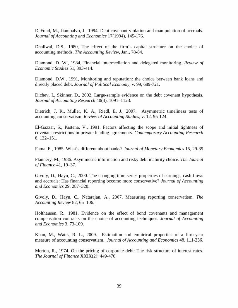
39
DeFond, M., Jiambalvo, J., 1994. Debt covenant violation and manipulation of accruals. Journal of Accounting and Economics 17(1994), 145-176. Dhaliwal, D.S., 1980, The effect of the firm’s capital structure on the choice of accounting methods. The Accounting Review, Jan., 78-84. Diamond, D. W., 1984, Financial intermediation and delegated monitoring. Review of Economic Studies 51, 393-414. Diamond, D.W., 1991, Monitoring and reputation: the choice between bank loans and directly placed debt. Journal of Political Economy, v. 99, 689-721. Dichev, I., Skinner, D., 2002. Large-sample evidence on the debt covenant hypothesis. Journal of Accounting Research 40(4), 1091–1123. Dietrich, J. R., Muller, K. A., Riedl, E. J., 2007. Asymmetric timeliness tests of accounting conservatism. Review of Accounting Studies, v. 12. 95-124. El-Gazzar, S., Pastena, V., 1991. Factors affecting the scope and initial tightness of covenant restrictions in private lending agreements. Contemporary Accounting Research 8, 132–151. Fama, E., 1985. What’s different about banks? Journal of Monetary Economics 15, 29-39. Flannery, M., 1986. Asymmetric information and risky debt maturity choice. The Journal of Finance 41, 19–37. Givoly, D., Hayn, C., 2000. The changing time-series properties of earnings, cash flows and accruals: Has financial reporting become more conservative? Journal of Accounting and Economics 29, 287–320. Givoly, D., Hayn, C., Natarajan, A., 2007. Measuring reporting conservatism. The Accounting Review 82, 65–106. Holthausen, R., 1981. Evidence on the effect of bond covenants and management compensation contracts on the choice of accounting techniques. Journal of Accounting and Economics 3, 73-109. Khan, M., Watts, R. L., 2009. Estimation and empirical properties of a firm-year measure of accounting conservatism. Journal of Accounting and Economics 48, 111-236. Merton, R., 1974. On the pricing of corporate debt: The risk structure of interest rates. The Journal of Finance XXIX(2): 449-470.

40
Moerman, R. W., 2008. The role of information asymmetry and financial reporting quality in debt trading: Evidence from the secondary loan market. Journal of Accounting and Economics 46, 240-260. Ramakrishnan, R. T. S., Thakor, A. V., 1984. Information Reliability and a Theory of Financial Intermediation. Review of Economic Studies, 51, 415-432. Roychowdhury, S., Watts, R. L., 2007. Asymmetric timeliness of earnings, market-to-book and conservatism in financial reporting. Journal of Accounting and Economics, 44(1–2), 2–31. Roberts, M., Sufi, A., 2008. Renegotiation of financial contracts: Evidence from private credit agreements. Working paper. University of Pennsylvania and University of Chicago. Sharpe, Steven, 1990, Asymmetric information, bank lending, and implicit contracts: A stylized model of customer relationship, The Journal of Finance 45, 1069-1087. Smith, Clifford W., 1993. A perspective on accounting-based debt covenant violations, The Accounting Review 68, 289-303. Smith, C., Warner, J., 1979. On financial contracting: an analysis of bond covenants, Journal of Financial Economics 7, 117–161. Standard & Poor’s, September 2006. A Guide To The Loan Market. Sufi, A., 2007, Information asymmetry and financing arrangements: Evidence from syndicated loans, The Journal of Finance, Vol. LXII, No. 2, 629-668. Sweeney, A., 1994. Debt-covenant violations and managers’ accounting responses. Journal of Accounting and Economics 17, 281–308. Watts, R., 2003a. Conservatism in accounting, Part I: Explanations and implications. Accounting Horizons 17, 207–221. Watts, R., 2003b. Conservatism in accounting, Part II: Evidence and research opportunities. Accounting Horizons 17, 287–301. Watts, R., Zimmerman, J., 1986. Positive Accounting Theory. Prentice-Hall, Englewood Cliffs, NJ. Zhang, J., 2008. The contracting benefits of accounting conservatism to lenders and borrowers. Journal of Accounting and Economics 45, 27-54.

Table 1. Sample Selection Process
The sample is drawn from Dealscan, provided by LPC. I extracted all private loans with net worth covenants and loan active dates between 1990 and 2005. Financial statement information was obtained from COMPUSTAT, and stock return information was obtained from CRSP. Panel A. Sample for Asymmetric Timeliness Measure
Number of firms
Number of firm-years
Loans with net worth covenants 5,385
After matching with COMPUSTAT/CRSP 1,287 3,252
After excluding firms with no earnings or returns data at t 1,183 3,003
After excluding firms with no earnings or return data at t − 1 or t + 1 1,061 2,716
After excluding outliers (top and bottom 0.5% of firms) 1,042 2,666
After excluding firms with tenure of less than 24 months 945 2,092
After excluding firms with slack less than or equal to 0 778 1,582 After including only the loan with the lowest net worth covenant in the same year for the same firm
778 1,150
Final sample 778 1,150
Panel B. Sample for Accruals Measure
Number of firms
Number of firm-years
Loans with net worth covenants 5,385
After matching with COMPUSTAT/CRSP 1,387 3,586
After excluding firms with no nonoperating accruals data at t 1,182 3,068
After excluding firms with no nonoperating accruals data at t + 1 1,153 3,004
After excluding outliers (top and bottom 0.5% of firms) 1,143 2,975
After excluding firms with tenure of less than 24 months 1,040 2,412
After excluding firms with slack less than or equal to 0 824 1,731 After including only the loan with the lowest net worth covenant in the same year for the same firm
824 1,207
Final sample 824 1,207
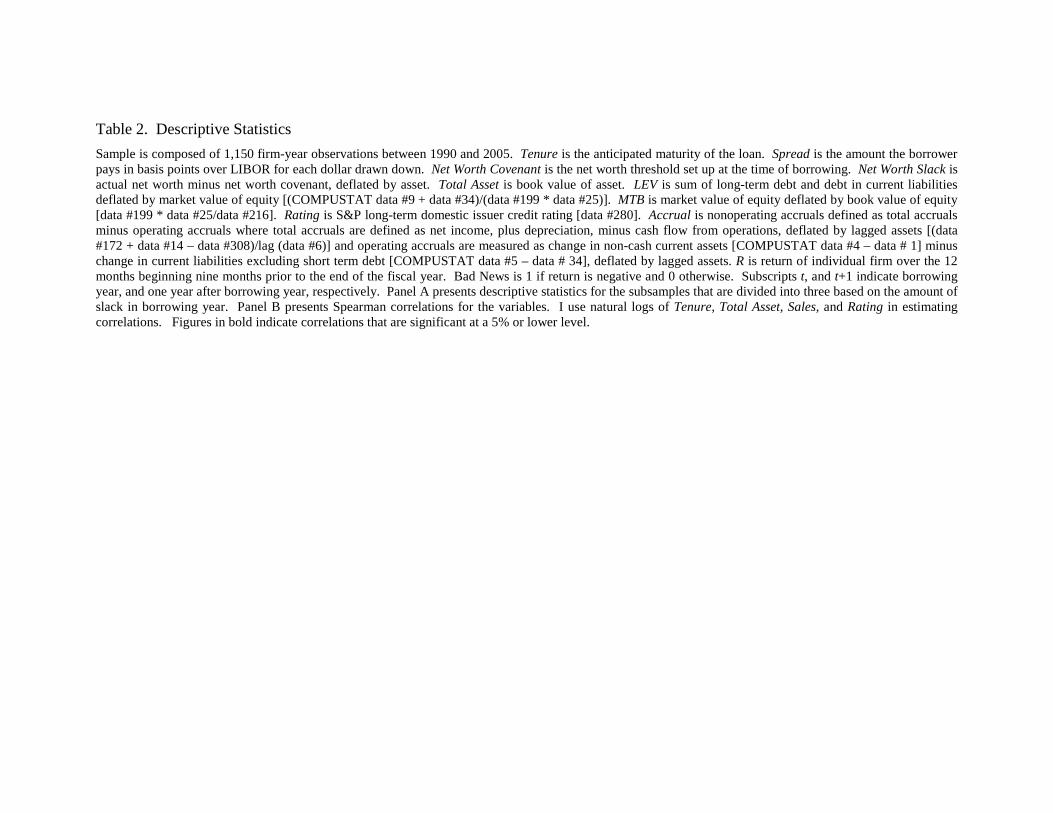
Table 2. Descriptive Statistics
Sample is composed of 1,150 firm-year observations between 1990 and 2005. Tenure is the anticipated maturity of the loan. Spread is the amount the borrower pays in basis points over LIBOR for each dollar drawn down. Net Worth Covenant is the net worth threshold set up at the time of borrowing. Net Worth Slack is actual net worth minus net worth covenant, deflated by asset. Total Asset is book value of asset. LEV is sum of long-term debt and debt in current liabilities deflated by market value of equity [(COMPUSTAT data #9 + data #34)/(data #199 * data #25)]. MTB is market value of equity deflated by book value of equity [data #199 * data #25/data #216]. Rating is S&P long-term domestic issuer credit rating [data #280]. Accrual is nonoperating accruals defined as total accruals minus operating accruals where total accruals are defined as net income, plus depreciation, minus cash flow from operations, deflated by lagged assets [(data #172 + data #14 – data #308)/lag (data #6)] and operating accruals are measured as change in non-cash current assets [COMPUSTAT data #4 – data # 1] minus change in current liabilities excluding short term debt [COMPUSTAT data #5 – data # 34], deflated by lagged assets. R is return of individual firm over the 12 months beginning nine months prior to the end of the fiscal year. Bad News is 1 if return is negative and 0 otherwise. Subscripts t, and t+1 indicate borrowing year, and one year after borrowing year, respectively. Panel A presents descriptive statistics for the subsamples that are divided into three based on the amount of slack in borrowing year. Panel B presents Spearman correlations for the variables. I use natural logs of Tenure, Total Asset, Sales, and Rating in estimating correlations. Figures in bold indicate correlations that are significant at a 5% or lower level.
Panel A. Descriptive Statistics
Mean Median Std. Mean Median Std. Mean Median Std.
Tenure (Month) 48.8 48.0 16.1 50.1 50.0 17.4 52.0 58.0 21.1
Spread 176.8 175.0 94.2 146.7 125.0 95.6 147.4 112.2 124.2
Net Worth Covenant (MM$) 576.3 174.0 1769.4 540.6 220.0 1416.0 469.3 175.0 1249.1
Net Worth Slack 0.027 0.026 0.015 0.077 0.076 0.015 0.205 0.168 0.105
Loan amount (MM$) 298.4 150.0 531.8 340.8 177.5 675.1 308.9 150.0 507.3
Total Assett (MM$) 5,150.9 552.0 29,223.5 2,382.0 608.1 7,499.3 2,124.0 574.7 5,128.1
Salest (MM$) 1,633.2 487.4 4,438.4 1,539.3 587.4 3,155.3 1,952.3 536.3 5,407.1
LEVt 0.83 0.45 1.16 0.55 0.30 1.05 0.34 0.18 0.54
MTBt 2.35 1.69 3.70 2.21 1.81 1.53 2.42 2.03 1.80
Ratingt 12.82 13.00 2.66 11.97 12.00 2.37 10.91 11.00 3.18
Accrualt -0.027 -0.012 0.083 -0.031 -0.016 0.079 -0.015 -0.011 0.070
Rt 0.21 0.11 0.63 0.20 0.13 0.52 0.12 0.08 0.42
Bad Newst 0.40 0.00 0.49 0.36 0.00 0.48 0.42 0.00 0.05
Bad Newst+1 0.35 0.00 0.48 0.41 0.00 0.49 0.38 0.00 0.49
Low Slack Medium Slack High Slack
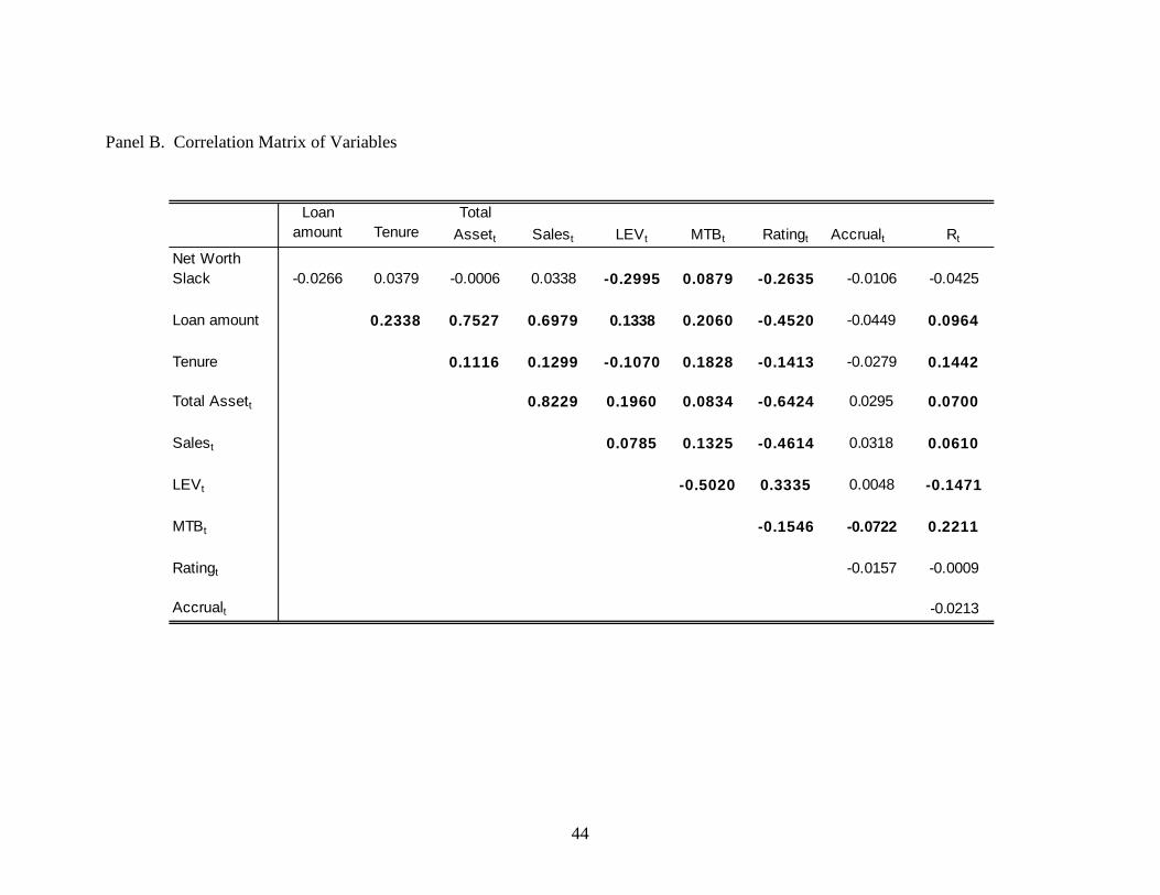
44
Panel B. Correlation Matrix of Variables
Loan amount Tenure
Total
Assett Salest LEVt MTBt Ratingt Accrualt Rt
Net Worth Slack -0.0266 0.0379 -0.0006 0.0338 -0.2995 0.0879 -0.2635 -0.0106 -0.0425
Loan amount 0.2338 0.7527 0.6979 0.1338 0.2060 -0.4520 -0.0449 0.0964
Tenure 0.1116 0.1299 -0.1070 0.1828 -0.1413 -0.0279 0.1442
Total Assett 0.8229 0.1960 0.0834 -0.6424 0.0295 0.0700
Salest 0.0785 0.1325 -0.4614 0.0318 0.0610
LEVt -0.5020 0.3335 0.0048 -0.1471
MTBt -0.1546 -0.0722 0.2211
Ratingt -0.0157 -0.0009
Accrualt -0.0213
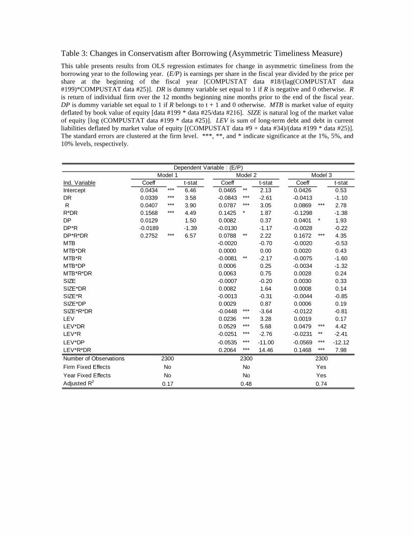
Table 3: Changes in Conservatism after Borrowing (Asymmetric Timeliness Measure)
This table presents results from OLS regression estimates for change in asymmetric timeliness from the borrowing year to the following year. (E/P) is earnings per share in the fiscal year divided by the price per share at the beginning of the fiscal year [COMPUSTAT data #18/(lag(COMPUSTAT data #199)*COMPUSTAT data #25)]. DR is dummy variable set equal to 1 if R is negative and 0 otherwise. R is return of individual firm over the 12 months beginning nine months prior to the end of the fiscal year. DP is dummy variable set equal to 1 if R belongs to t + 1 and 0 otherwise. MTB is market value of equity deflated by book value of equity [data #199 * data #25/data #216]. SIZE is natural log of the market value of equity [log (COMPUSTAT data #199 * data #25)]. LEV is sum of long-term debt and debt in current liabilities deflated by market value of equity [(COMPUSTAT data #9 + data #34)/(data #199 * data #25)]. The standard errors are clustered at the firm level. ***, **, and * indicate significance at the 1%, 5%, and 10% levels, respectively.
Ind. Variable Coeff t-stat Coeff t-stat Coeff t-statIntercept 0.0434 *** 6.46 0.0465 ** 2.13 0.0426 0.53DR 0.0339 *** 3.58 -0.0843 *** -2.61 -0.0413 -1.10 R 0.0407 *** 3.90 0.0787 *** 3.05 0.0869 *** 2.78R*DR 0.1568 *** 4.49 0.1425 * 1.87 -0.1298 -1.38DP 0.0129 1.50 0.0082 0.37 0.0401 * 1.93DP*R -0.0189 -1.39 -0.0130 -1.17 -0.0028 -0.22DP*R*DR 0.2752 *** 6.57 0.0788 ** 2.22 0.1672 *** 4.35MTB -0.0020 -0.70 -0.0020 -0.53MTB*DR 0.0000 0.00 0.0020 0.43MTB*R -0.0081 ** -2.17 -0.0075 -1.60MTB*DP 0.0006 0.25 -0.0034 -1.32MTB*R*DR 0.0063 0.75 0.0028 0.24SIZE -0.0007 -0.20 0.0030 0.33SIZE*DR 0.0082 1.64 0.0008 0.14SIZE*R -0.0013 -0.31 -0.0044 -0.85SIZE*DP 0.0029 0.87 0.0006 0.19SIZE*R*DR -0.0448 *** -3.64 -0.0122 -0.81LEV 0.0236 *** 3.28 0.0019 0.17LEV*DR 0.0529 *** 5.68 0.0479 *** 4.42LEV*R -0.0251 *** -2.76 -0.0231 ** -2.41
LEV*DP -0.0535 *** -11.00 -0.0569 *** -12.12LEV*R*DR 0.2064 *** 14.46 0.1468 *** 7.98
Number of Observations
Firm Fixed Effects
Year Fixed EffectsAdjusted R2
Yes
Yes
0.74
Model 3
2300
Dependent Variable : (E/P)
0.17 0.48
No No
No No
Model 1 Model 2
2300 2300
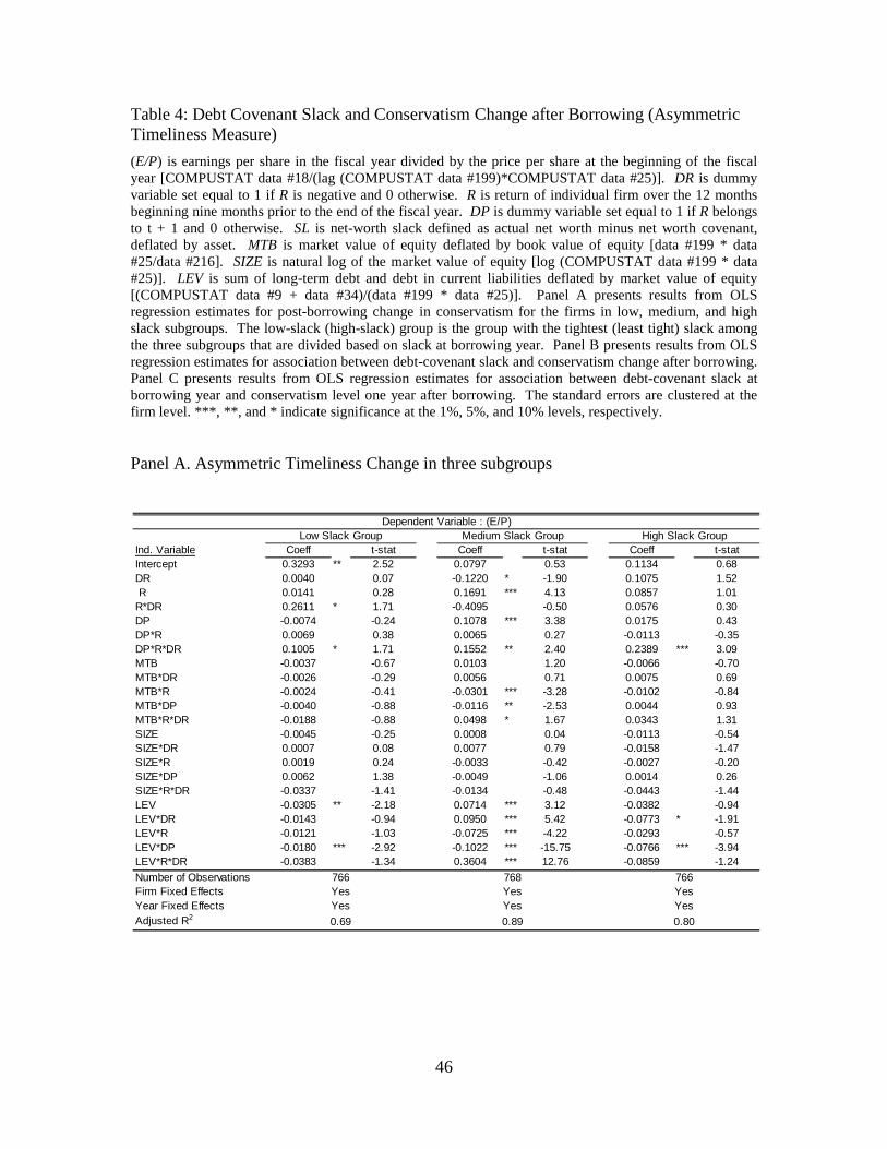
46
Table 4: Debt Covenant Slack and Conservatism Change after Borrowing (Asymmetric Timeliness Measure)
(E/P) is earnings per share in the fiscal year divided by the price per share at the beginning of the fiscal year [COMPUSTAT data #18/(lag (COMPUSTAT data #199)*COMPUSTAT data #25)]. DR is dummy variable set equal to 1 if R is negative and 0 otherwise. R is return of individual firm over the 12 months beginning nine months prior to the end of the fiscal year. DP is dummy variable set equal to 1 if R belongs to t + 1 and 0 otherwise. SL is net-worth slack defined as actual net worth minus net worth covenant, deflated by asset. MTB is market value of equity deflated by book value of equity [data #199 * data #25/data #216]. SIZE is natural log of the market value of equity [log (COMPUSTAT data #199 * data #25)]. LEV is sum of long-term debt and debt in current liabilities deflated by market value of equity [(COMPUSTAT data #9 + data #34)/(data #199 * data #25)]. Panel A presents results from OLS regression estimates for post-borrowing change in conservatism for the firms in low, medium, and high slack subgroups. The low-slack (high-slack) group is the group with the tightest (least tight) slack among the three subgroups that are divided based on slack at borrowing year. Panel B presents results from OLS regression estimates for association between debt-covenant slack and conservatism change after borrowing. Panel C presents results from OLS regression estimates for association between debt-covenant slack at borrowing year and conservatism level one year after borrowing. The standard errors are clustered at the firm level. ***, **, and * indicate significance at the 1%, 5%, and 10% levels, respectively. Panel A. Asymmetric Timeliness Change in three subgroups
Ind. Variable Coeff t-stat Coeff t-stat Coeff t-statIntercept 0.3293 ** 2.52 0.0797 0.53 0.1134 0.68DR 0.0040 0.07 -0.1220 * -1.90 0.1075 1.52 R 0.0141 0.28 0.1691 *** 4.13 0.0857 1.01R*DR 0.2611 * 1.71 -0.4095 -0.50 0.0576 0.30DP -0.0074 -0.24 0.1078 *** 3.38 0.0175 0.43DP*R 0.0069 0.38 0.0065 0.27 -0.0113 -0.35DP*R*DR 0.1005 * 1.71 0.1552 ** 2.40 0.2389 *** 3.09MTB -0.0037 -0.67 0.0103 1.20 -0.0066 -0.70MTB*DR -0.0026 -0.29 0.0056 0.71 0.0075 0.69MTB*R -0.0024 -0.41 -0.0301 *** -3.28 -0.0102 -0.84MTB*DP -0.0040 -0.88 -0.0116 ** -2.53 0.0044 0.93MTB*R*DR -0.0188 -0.88 0.0498 * 1.67 0.0343 1.31SIZE -0.0045 -0.25 0.0008 0.04 -0.0113 -0.54SIZE*DR 0.0007 0.08 0.0077 0.79 -0.0158 -1.47SIZE*R 0.0019 0.24 -0.0033 -0.42 -0.0027 -0.20SIZE*DP 0.0062 1.38 -0.0049 -1.06 0.0014 0.26SIZE*R*DR -0.0337 -1.41 -0.0134 -0.48 -0.0443 -1.44LEV -0.0305 ** -2.18 0.0714 *** 3.12 -0.0382 -0.94LEV*DR -0.0143 -0.94 0.0950 *** 5.42 -0.0773 * -1.91LEV*R -0.0121 -1.03 -0.0725 *** -4.22 -0.0293 -0.57LEV*DP -0.0180 *** -2.92 -0.1022 *** -15.75 -0.0766 *** -3.94LEV*R*DR -0.0383 -1.34 0.3604 *** 12.76 -0.0859 -1.24
Number of ObservationsFirm Fixed EffectsYear Fixed EffectsAdjusted R2
Yes Yes
0.69 0.89
Low Slack Group Medium Slack Group
766 768Yes Yes
High Slack Group
766YesYes
0.80
Dependent Variable : (E/P)
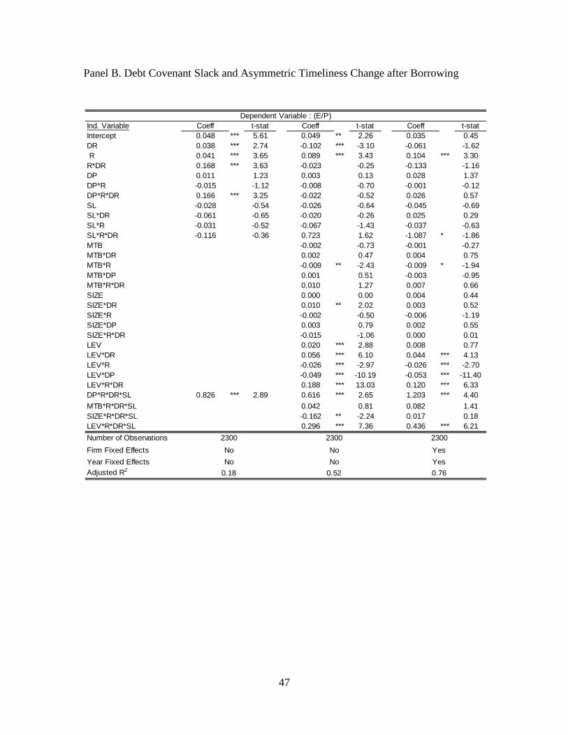
47
Panel B. Debt Covenant Slack and Asymmetric Timeliness Change after Borrowing
Ind. Variable Coeff t-stat Coeff t-stat Coeff t-statIntercept 0.048 *** 5.61 0.049 ** 2.26 0.035 0.45DR 0.038 *** 2.74 -0.102 *** -3.10 -0.061 -1.62 R 0.041 *** 3.65 0.089 *** 3.43 0.104 *** 3.30R*DR 0.168 *** 3.63 -0.023 -0.25 -0.133 -1.16DP 0.011 1.23 0.003 0.13 0.028 1.37DP*R -0.015 -1.12 -0.008 -0.70 -0.001 -0.12DP*R*DR 0.166 *** 3.25 -0.022 -0.52 0.026 0.57SL -0.028 -0.54 -0.026 -0.64 -0.045 -0.69SL*DR -0.061 -0.65 -0.020 -0.26 0.025 0.29SL*R -0.031 -0.52 -0.067 -1.43 -0.037 -0.63SL*R*DR -0.116 -0.36 0.723 1.62 -1.087 * -1.86MTB -0.002 -0.73 -0.001 -0.27MTB*DR 0.002 0.47 0.004 0.75MTB*R -0.009 ** -2.43 -0.009 * -1.94MTB*DP 0.001 0.51 -0.003 -0.95MTB*R*DR 0.010 1.27 0.007 0.66SIZE 0.000 0.00 0.004 0.44SIZE*DR 0.010 ** 2.02 0.003 0.52SIZE*R -0.002 -0.50 -0.006 -1.19SIZE*DP 0.003 0.79 0.002 0.55SIZE*R*DR -0.015 -1.06 0.000 0.01LEV 0.020 *** 2.88 0.008 0.77LEV*DR 0.056 *** 6.10 0.044 *** 4.13LEV*R -0.026 *** -2.97 -0.026 *** -2.70LEV*DP -0.049 *** -10.19 -0.053 *** -11.40LEV*R*DR 0.188 *** 13.03 0.120 *** 6.33DP*R*DR*SL 0.826 *** 2.89 0.616 *** 2.65 1.203 *** 4.40
MTB*R*DR*SL 0.042 0.81 0.082 1.41SIZE*R*DR*SL -0.162 ** -2.24 0.017 0.18LEV*R*DR*SL 0.296 *** 7.36 0.436 *** 6.21
Number of Observations
Firm Fixed Effects
Year Fixed EffectsAdjusted R2
2300
No
No
0.520.18
Dependent Variable : (E/P)
2300
Yes
Yes
0.76
2300
No
No
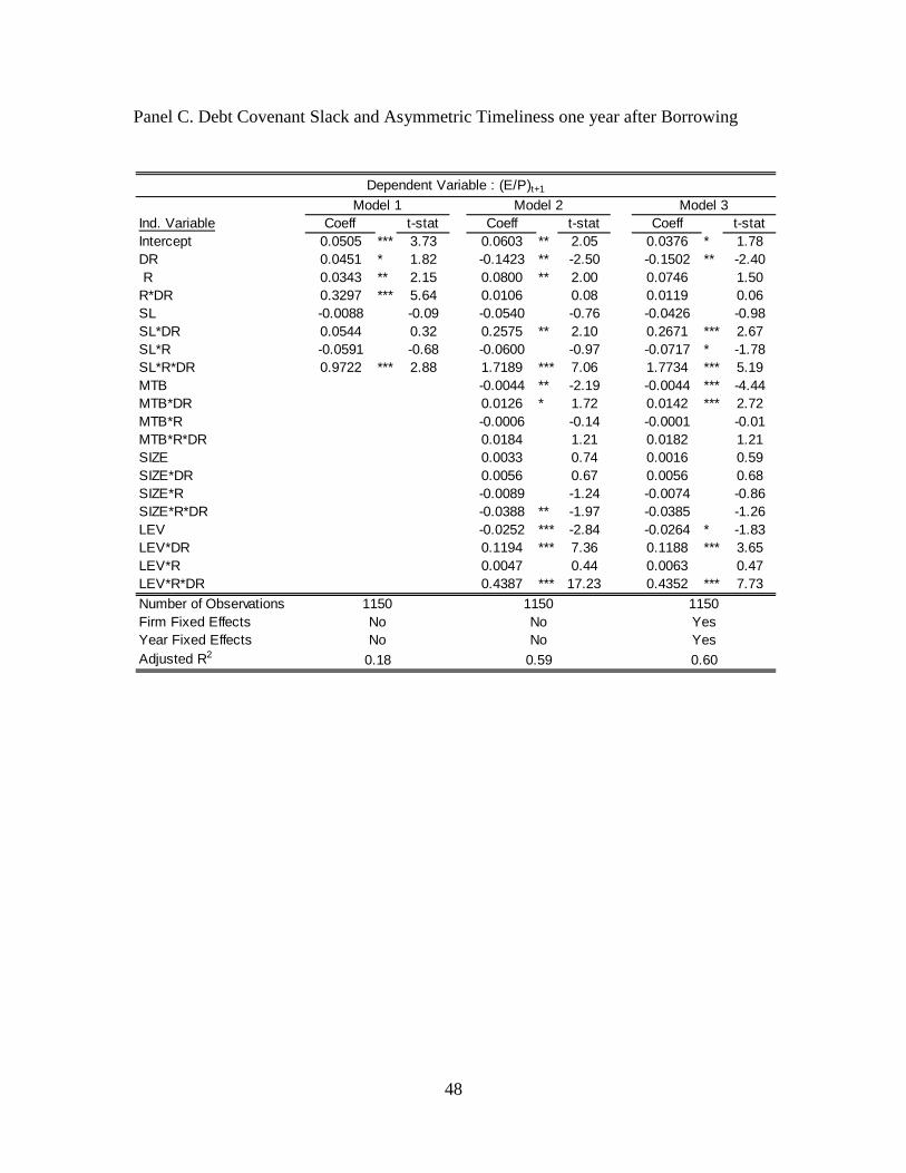
48
Panel C. Debt Covenant Slack and Asymmetric Timeliness one year after Borrowing
Ind. Variable Coeff t-stat Coeff t-stat Coeff t-statIntercept 0.0505 *** 3.73 0.0603 ** 2.05 0.0376 * 1.78DR 0.0451 * 1.82 -0.1423 ** -2.50 -0.1502 ** -2.40 R 0.0343 ** 2.15 0.0800 ** 2.00 0.0746 1.50R*DR 0.3297 *** 5.64 0.0106 0.08 0.0119 0.06SL -0.0088 -0.09 -0.0540 -0.76 -0.0426 -0.98SL*DR 0.0544 0.32 0.2575 ** 2.10 0.2671 *** 2.67SL*R -0.0591 -0.68 -0.0600 -0.97 -0.0717 * -1.78SL*R*DR 0.9722 *** 2.88 1.7189 *** 7.06 1.7734 *** 5.19MTB -0.0044 ** -2.19 -0.0044 *** -4.44MTB*DR 0.0126 * 1.72 0.0142 *** 2.72MTB*R -0.0006 -0.14 -0.0001 -0.01MTB*R*DR 0.0184 1.21 0.0182 1.21SIZE 0.0033 0.74 0.0016 0.59SIZE*DR 0.0056 0.67 0.0056 0.68SIZE*R -0.0089 -1.24 -0.0074 -0.86SIZE*R*DR -0.0388 ** -1.97 -0.0385 -1.26LEV -0.0252 *** -2.84 -0.0264 * -1.83LEV*DR 0.1194 *** 7.36 0.1188 *** 3.65LEV*R 0.0047 0.44 0.0063 0.47LEV*R*DR 0.4387 *** 17.23 0.4352 *** 7.73
Number of ObservationsFirm Fixed EffectsYear Fixed EffectsAdjusted R2 0.18 0.59 0.60
No No YesNo No Yes
1150 1150 1150
Dependent Variable : (E/P)t+1
Model 1 Model 2 Model 3
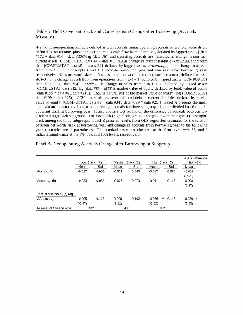
49
Table 5: Debt Covenant Slack and Conservatism Change after Borrowing (Accruals Measure) Accrual is nonoperating accruals defined as total accruals minus operating accruals where total accruals are defined as net income, plus depreciation, minus cash flow from operations, deflated by lagged assets [(data #172 + data #14 – data #308)/lag (data #6)] and operating accruals are measured as change in non-cash current assets [COMPUSTAT data #4 – data # 1] minus change in current liabilities excluding short term debt [COMPUSTAT data #5 – data # 34], deflated by lagged assets. ∆Accrualt,t+1 is the change in accrual from t to t + 1. Subscripts t and t+1 indicate borrowing year and one year after borrowing year, respectively. SL is net-worth slack defined as actual net worth minus net worth covenant, deflated by asset. ∆CFO t, t+1 is change in cash flow from operations from t to t + 1, deflated by lagged assets [COMPUSTAT data #308/ lag (data #6)]. ∆Salet,t+1 is change in sales from t to t + 1, deflated by lagged assets [COMPUSTAT data #12/ lag (data #6)]. MTB is market value of equity deflated by book value of equity [data #199 * data #25/data #216]. SIZE is natural log of the market value of equity [log (COMPUSTAT data #199 * data #25)]. LEV is sum of long-term debt and debt in current liabilities deflated by market value of equity [(COMPUSTAT data #9 + data #34)/(data #199 * data #25)]. Panel A presents the mean and standard deviation values of nonoperating accruals for three subgroups that are divided based on debt covenant slack at borrowing year. It also shows t-test results on the difference of accruals between low slack and high slack subgroups. The low-slack (high-slack) group is the group with the tightest (least tight) slack among the three subgroups. Panel B presents results from OLS regression estimates for the relation between net worth slack at borrowing year and change in accruals from borrowing year to the following year. t-statistics are in parentheses. The standard errors are clustered at the firm level. ***, **, and * indicate significance at the 1%, 5%, and 10% levels, respectively. Panel A. Nonoperating Accruals Change after Borrowing in Subgroup
Mean Std Mean Std Mean Std Mean
Accrualt (a) -0.027 0.083 -0.031 0.080 -0.015 0.070 -0.012 **
(-2.29)
Accrualt+1 (b) -0.033 0.082 -0.026 0.073 -0.041 0.143 0.008
(0.97)
Test of difference [(b)-(a)]
∆Accrual t, t+1 -0.005 0.112 0.006 0.102 -0.026 *** 0.143 0.020 **
(-0.97) (1.12) (-3.62) (2.25)
Number of Observations
Low Slack (A) High Slack (C)Test of difference
[(A)-(C)]
402 402
Medium Slack (B)
403
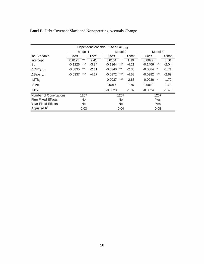
50
Panel B. Debt Covenant Slack and Nonoperating Accruals Change
Ind. Variable Coeff t-stat Coeff t-stat Coeff t-statIntercept 0.0125 ** 2.41 0.0164 1.19 0.0079 0.50SL -0.1226 *** -3.84 -0.1364 *** -4.21 -0.1406 ** -2.04
∆CFOt, t+1 -0.0835 ** -2.11 -0.0940 ** -2.35 -0.0864 * -1.71
∆Salet, t+1 -0.0337 *** -4.27 -0.0372 *** -4.58 -0.0382 *** -2.69
MTBt -0.0037 *** -2.88 -0.0036 * -1.72
Sizet 0.0017 0.76 0.0010 0.41
LEVt -0.0023 -1.37 -0.0024 -1.46
Number of ObservationsFirm Fixed EffectsYear Fixed EffectsAdjusted R2
Dependent Variable : ∆Accrual t, t+1
Model 1 Model 2 Model 3
1207 1207 1207No No YesNo No Yes
0.03 0.04 0.05
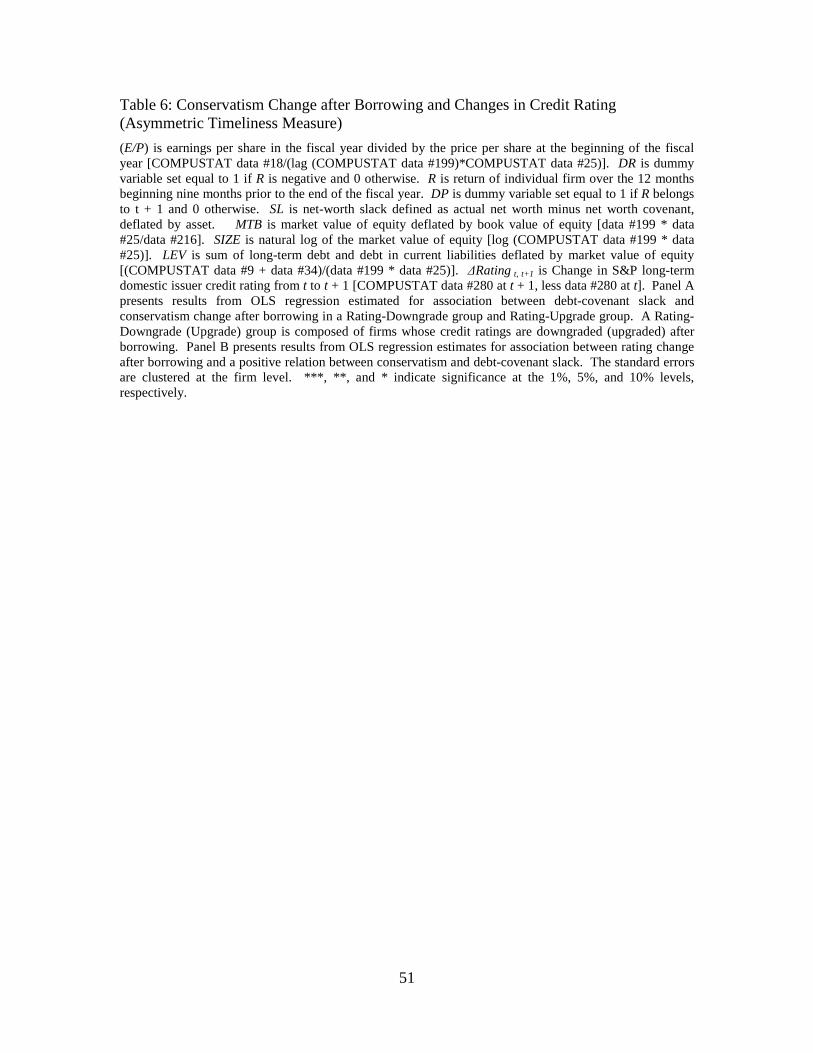
51
Table 6: Conservatism Change after Borrowing and Changes in Credit Rating (Asymmetric Timeliness Measure)
(E/P) is earnings per share in the fiscal year divided by the price per share at the beginning of the fiscal year [COMPUSTAT data #18/(lag (COMPUSTAT data #199)*COMPUSTAT data #25)]. DR is dummy variable set equal to 1 if R is negative and 0 otherwise. R is return of individual firm over the 12 months beginning nine months prior to the end of the fiscal year. DP is dummy variable set equal to 1 if R belongs to t + 1 and 0 otherwise. SL is net-worth slack defined as actual net worth minus net worth covenant, deflated by asset. MTB is market value of equity deflated by book value of equity [data #199 * data #25/data #216]. SIZE is natural log of the market value of equity [log (COMPUSTAT data #199 * data #25)]. LEV is sum of long-term debt and debt in current liabilities deflated by market value of equity [(COMPUSTAT data #9 + data #34)/(data #199 * data #25)]. ∆Rating t, t+1 is Change in S&P long-term domestic issuer credit rating from t to t + 1 [COMPUSTAT data #280 at t + 1, less data #280 at t]. Panel A presents results from OLS regression estimated for association between debt-covenant slack and conservatism change after borrowing in a Rating-Downgrade group and Rating-Upgrade group. A Rating-Downgrade (Upgrade) group is composed of firms whose credit ratings are downgraded (upgraded) after borrowing. Panel B presents results from OLS regression estimates for association between rating change after borrowing and a positive relation between conservatism and debt-covenant slack. The standard errors are clustered at the firm level. ***, **, and * indicate significance at the 1%, 5%, and 10% levels, respectively.
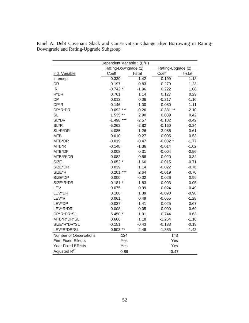
52
Panel A. Debt Covenant Slack and Conservatism Change after Borrowing in Rating-Downgrade and Rating-Upgrade Subgroup
Ind. Variable Coeff t-stat Coeff t-statIntercept 0.330 1.42 0.199 1.18DR -0.197 -0.83 0.279 1.23 R -0.742 * -1.96 0.222 1.08R*DR 0.761 1.14 0.127 0.29DP 0.012 0.06 -0.217 -1.16DP*R -0.146 -1.00 0.080 1.11DP*R*DR -0.092 *** -0.26 -0.331 ** -2.10SL 1.535 ** 2.90 0.089 0.42SL*DR -1.498 *** -2.57 -0.102 -0.42SL*R -5.262 -2.82 -0.160 -0.34SL*R*DR 4.085 1.26 3.986 0.61MTB 0.010 0.27 0.005 0.53MTB*DR -0.019 -0.47 -0.032 * -1.77MTB*R -0.148 -1.36 -0.014 -1.02MTB*DP 0.008 0.31 -0.004 -0.56MTB*R*DR 0.082 0.58 0.020 0.34SIZE -0.052 * -1.66 -0.015 -0.71SIZE*DR 0.039 1.14 -0.022 -0.76SIZE*R 0.201 *** 2.64 -0.019 -0.70SIZE*DP 0.000 -0.02 0.026 0.99SIZE*R*DR -0.181 * -1.83 0.003 0.05LEV -0.075 -0.99 -0.024 -0.49LEV*DR 0.106 1.39 -0.090 -0.98LEV*R 0.061 0.49 -0.055 -1.28LEV*DP -0.037 -1.41 0.025 0.67LEV*R*DR 0.008 0.05 0.090 0.69DP*R*DR*SL 5.450 * 1.91 0.744 0.63MTB*R*DR*SL 0.666 1.18 -1.264 -1.16SIZE*R*DR*SL -0.151 -0.43 -0.183 -0.19LEV*R*DR*SL 0.503 ** 2.48 -1.385 -1.42
Number of ObservationsFirm Fixed EffectsYear Fixed EffectsAdjusted R2
Yes
0.86 0.47
Dependent Variable : (E/P)Rating-Downgrade (1) Rating-Upgrade (2)
124 143Yes YesYes
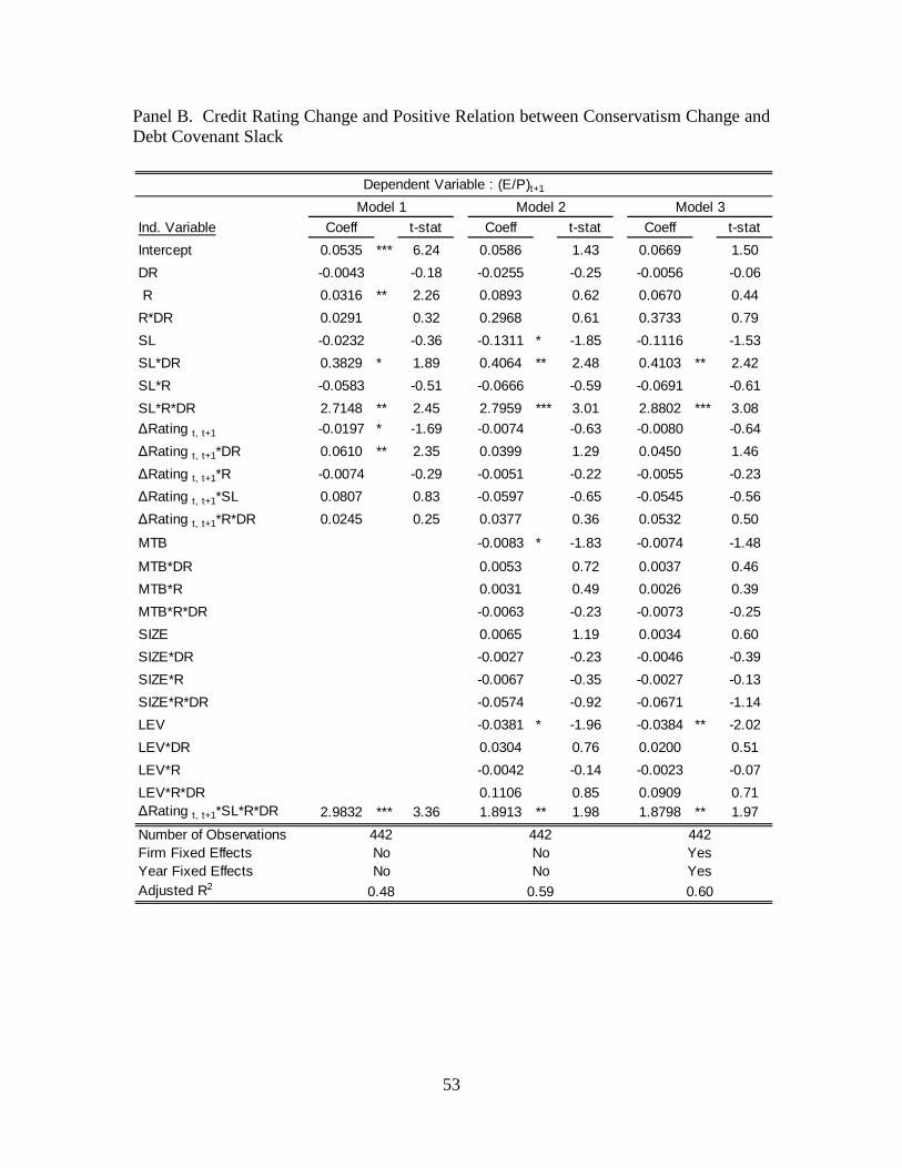
53
Panel B. Credit Rating Change and Positive Relation between Conservatism Change and Debt Covenant Slack
Ind. Variable Coeff t-stat Coeff t-stat Coeff t-stat
Intercept 0.0535 *** 6.24 0.0586 1.43 0.0669 1.50
DR -0.0043 -0.18 -0.0255 -0.25 -0.0056 -0.06
R 0.0316 ** 2.26 0.0893 0.62 0.0670 0.44
R*DR 0.0291 0.32 0.2968 0.61 0.3733 0.79
SL -0.0232 -0.36 -0.1311 * -1.85 -0.1116 -1.53
SL*DR 0.3829 * 1.89 0.4064 ** 2.48 0.4103 ** 2.42
SL*R -0.0583 -0.51 -0.0666 -0.59 -0.0691 -0.61
SL*R*DR 2.7148 ** 2.45 2.7959 *** 3.01 2.8802 *** 3.08
∆Rating t, t+1 -0.0197 * -1.69 -0.0074 -0.63 -0.0080 -0.64
∆Rating t, t+1*DR 0.0610 ** 2.35 0.0399 1.29 0.0450 1.46
∆Rating t, t+1*R -0.0074 -0.29 -0.0051 -0.22 -0.0055 -0.23
∆Rating t, t+1*SL 0.0807 0.83 -0.0597 -0.65 -0.0545 -0.56
∆Rating t, t+1*R*DR 0.0245 0.25 0.0377 0.36 0.0532 0.50
MTB -0.0083 * -1.83 -0.0074 -1.48
MTB*DR 0.0053 0.72 0.0037 0.46
MTB*R 0.0031 0.49 0.0026 0.39
MTB*R*DR -0.0063 -0.23 -0.0073 -0.25
SIZE 0.0065 1.19 0.0034 0.60
SIZE*DR -0.0027 -0.23 -0.0046 -0.39
SIZE*R -0.0067 -0.35 -0.0027 -0.13
SIZE*R*DR -0.0574 -0.92 -0.0671 -1.14
LEV -0.0381 * -1.96 -0.0384 ** -2.02
LEV*DR 0.0304 0.76 0.0200 0.51
LEV*R -0.0042 -0.14 -0.0023 -0.07
LEV*R*DR 0.1106 0.85 0.0909 0.71∆Rating t, t+1*SL*R*DR 2.9832 *** 3.36 1.8913 ** 1.98 1.8798 ** 1.97
Number of ObservationsFirm Fixed EffectsYear Fixed EffectsAdjusted R2 0.48 0.59 0.60
No No YesNo No Yes442 442 442
Dependent Variable : (E/P)t+1
Model 1 Model 2 Model 3
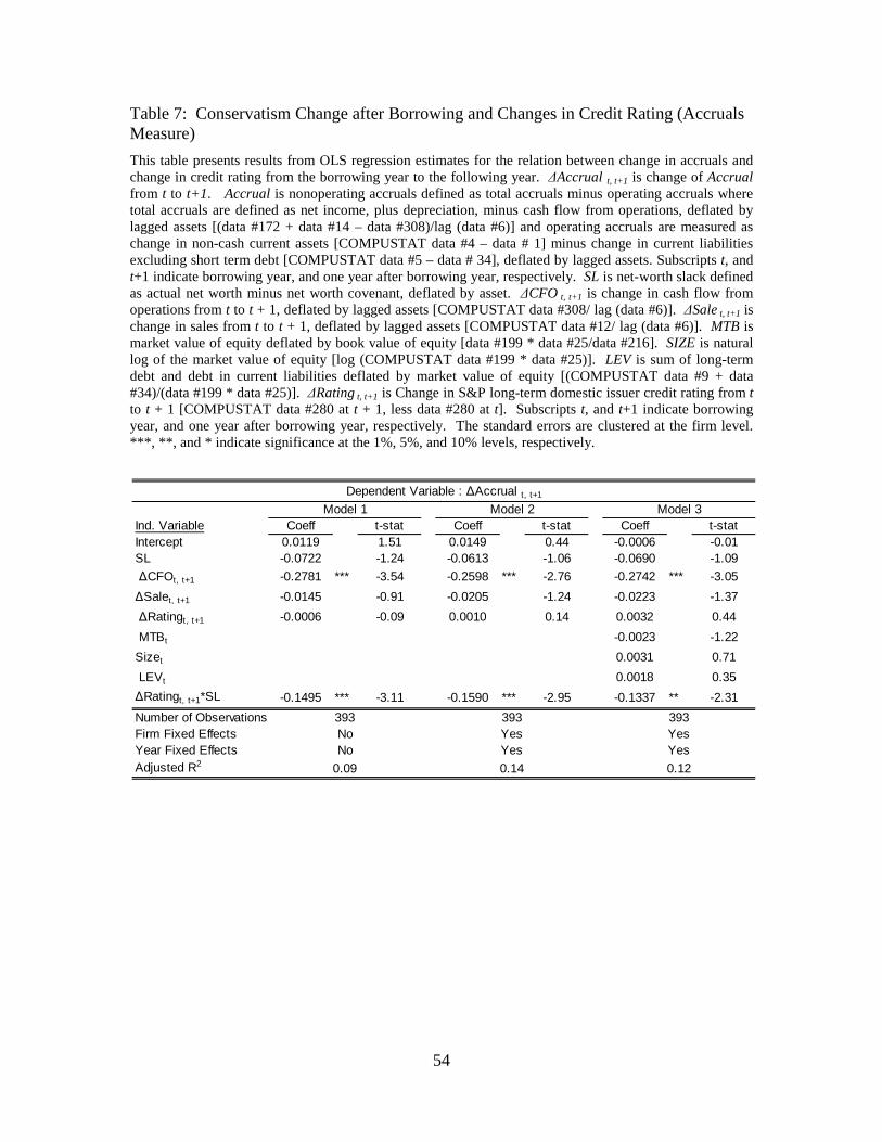
54
Table 7: Conservatism Change after Borrowing and Changes in Credit Rating (Accruals Measure)
This table presents results from OLS regression estimates for the relation between change in accruals and change in credit rating from the borrowing year to the following year. ∆Accrual t, t+1 is change of Accrual from t to t+1. Accrual is nonoperating accruals defined as total accruals minus operating accruals where total accruals are defined as net income, plus depreciation, minus cash flow from operations, deflated by lagged assets [(data #172 + data #14 – data #308)/lag (data #6)] and operating accruals are measured as change in non-cash current assets [COMPUSTAT data #4 – data # 1] minus change in current liabilities excluding short term debt [COMPUSTAT data #5 – data # 34], deflated by lagged assets. Subscripts t, and t+1 indicate borrowing year, and one year after borrowing year, respectively. SL is net-worth slack defined as actual net worth minus net worth covenant, deflated by asset. ∆CFO t, t+1 is change in cash flow from operations from t to t + 1, deflated by lagged assets [COMPUSTAT data #308/ lag (data #6)]. ∆Sale t, t+1 is change in sales from t to t + 1, deflated by lagged assets [COMPUSTAT data #12/ lag (data #6)]. MTB is market value of equity deflated by book value of equity [data #199 * data #25/data #216]. SIZE is natural log of the market value of equity [log (COMPUSTAT data #199 * data #25)]. LEV is sum of long-term debt and debt in current liabilities deflated by market value of equity [(COMPUSTAT data #9 + data #34)/(data #199 * data #25)]. ∆Rating t, t+1 is Change in S&P long-term domestic issuer credit rating from t to t + 1 [COMPUSTAT data #280 at t + 1, less data #280 at t]. Subscripts t, and t+1 indicate borrowing year, and one year after borrowing year, respectively. The standard errors are clustered at the firm level. ***, **, and * indicate significance at the 1%, 5%, and 10% levels, respectively.
Ind. Variable Coeff t-stat Coeff t-stat Coeff t-statIntercept 0.0119 1.51 0.0149 0.44 -0.0006 -0.01SL -0.0722 -1.24 -0.0613 -1.06 -0.0690 -1.09
∆CFOt, t+1 -0.2781 *** -3.54 -0.2598 *** -2.76 -0.2742 *** -3.05
∆Salet, t+1 -0.0145 -0.91 -0.0205 -1.24 -0.0223 -1.37
∆Ratingt, t+1 -0.0006 -0.09 0.0010 0.14 0.0032 0.44
MTBt -0.0023 -1.22
Sizet 0.0031 0.71
LEVt 0.0018 0.35
∆Ratingt, t+1*SL -0.1495 *** -3.11 -0.1590 *** -2.95 -0.1337 ** -2.31
Number of ObservationsFirm Fixed EffectsYear Fixed EffectsAdjusted R2
Dependent Variable : ∆Accrual t, t+1
Model 1 Model 2 Model 3
393 393 393No Yes YesNo Yes Yes
0.09 0.14 0.12
55
Table 8: Conservatism Change after Borrowing and Bank Monitoring (Asymmetric Timeliness Measure)
(E/P) is earnings per share in the fiscal year divided by the price per share at the beginning of the fiscal year [COMPUSTAT data #18/(lag (COMPUSTAT data #199)*COMPUSTAT data #25)]. DR is dummy variable set equal to 1 if R is negative and 0 otherwise. R is return of individual firm over the 12 months beginning nine months prior to the end of the fiscal year. DP is dummy variable set equal to 1 if R belongs to t + 1 and 0 otherwise. SL is net-worth slack defined as actual net worth minus net worth covenant, deflated by asset. MTB is market value of equity deflated by book value of equity [data #199 * data #25/data #216]. SIZE is natural log of the market value of equity [log (COMPUSTAT data #199 * data #25)]. LEV is sum of long-term debt and debt in current liabilities deflated by market value of equity [(COMPUSTAT data #9 + data #34)/(data #199 * data #25)]. Panel A presents results from OLS regression estimated for association between debt-covenant slack and conservatism change after borrowing in High/Low lead arranger portion. The High (Low) lead arranger portion group consists of firms whose loans have above (below) median lead arranger portion. Panel B presents results from OLS regression estimated for association between debt-covenant slack and conservatism change after borrowing in Small/Large number of lenders group. The Small (Large) number of lenders group consists of firms whose loans have above (below) median number of lenders. The standard errors are clustered at the firm level. ***, **, and * indicate significance at the 1%, 5%, and 10% levels, respectively.
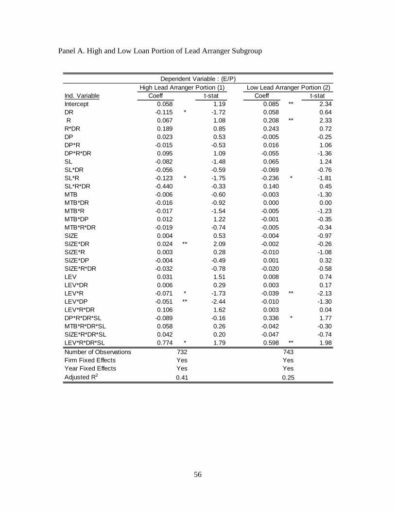
56
Panel A. High and Low Loan Portion of Lead Arranger Subgroup
Ind. Variable Coeff t-stat Coeff t-statIntercept 0.058 1.19 0.085 ** 2.34DR -0.115 * -1.72 0.058 0.64 R 0.067 1.08 0.208 ** 2.33R*DR 0.189 0.85 0.243 0.72DP 0.023 0.53 -0.005 -0.25DP*R -0.015 -0.53 0.016 1.06DP*R*DR 0.095 1.09 -0.055 -1.36SL -0.082 -1.48 0.065 1.24SL*DR -0.056 -0.59 -0.069 -0.76SL*R -0.123 * -1.75 -0.236 * -1.81SL*R*DR -0.440 -0.33 0.140 0.45MTB -0.006 -0.60 -0.003 -1.30MTB*DR -0.016 -0.92 0.000 0.00MTB*R -0.017 -1.54 -0.005 -1.23MTB*DP 0.012 1.22 -0.001 -0.35MTB*R*DR -0.019 -0.74 -0.005 -0.34SIZE 0.004 0.53 -0.004 -0.97SIZE*DR 0.024 ** 2.09 -0.002 -0.26SIZE*R 0.003 0.28 -0.010 -1.08SIZE*DP -0.004 -0.49 0.001 0.32SIZE*R*DR -0.032 -0.78 -0.020 -0.58LEV 0.031 1.51 0.008 0.74LEV*DR 0.006 0.29 0.003 0.17LEV*R -0.071 * -1.73 -0.039 ** -2.13LEV*DP -0.051 ** -2.44 -0.010 -1.30LEV*R*DR 0.106 1.62 0.003 0.04DP*R*DR*SL -0.089 -0.16 0.336 * 1.77MTB*R*DR*SL 0.058 0.26 -0.042 -0.30SIZE*R*DR*SL 0.042 0.20 -0.047 -0.74LEV*R*DR*SL 0.774 * 1.79 0.598 ** 1.98
Number of ObservationsFirm Fixed EffectsYear Fixed EffectsAdjusted R2
YesYes Yes
Dependent Variable : (E/P)High Lead Arranger Portion (1) Low Lead Arranger Portion (2)
0.41 0.25
732 743Yes
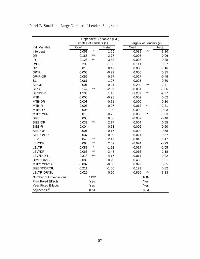
57
Panel B. Small and Large Number of Lenders Subgroup
Ind. Variable Coeff t-stat Coeff t-statIntercept 0.051 * 1.65 0.089 *** 3.20DR -0.183 *** -2.77 0.003 0.06 R 0.126 *** 3.83 -0.026 -0.38R*DR -0.299 -1.32 0.111 0.67DP 0.018 0.47 0.030 1.16DP*R -0.006 -0.29 0.006 0.35DP*R*DR 0.059 0.77 -0.027 -0.49SL -0.061 -1.27 0.025 0.80SL*DR -0.001 -0.01 -0.280 *** -2.71SL*R -0.142 ** -2.07 -0.051 -1.06SL*R*DR 1.535 1.46 -1.289 ** -2.37MTB -0.006 -0.98 0.002 0.52MTB*DR -0.008 -0.61 0.000 0.10MTB*R -0.006 -0.97 -0.012 ** -2.31MTB*DP 0.006 1.09 -0.002 -0.93MTB*R*DR -0.016 -0.75 0.036 * 1.83SIZE 0.000 0.06 -0.002 -0.46SIZE*DR 0.032 *** 2.77 0.004 0.55SIZE*R -0.004 -0.63 -0.006 -0.60SIZE*DP -0.001 -0.17 -0.002 -0.68SIZE*R*DR 0.037 0.89 -0.021 -0.57LEV 0.040 ** 2.17 0.016 1.47LEV*DR 0.063 ** 2.09 -0.024 -0.93LEV*R -0.081 * -1.92 -0.014 -1.05LEV*DP -0.065 *** -3.43 -0.016 -1.18LEV*R*DR 0.313 *** 4.17 -0.014 -0.22DP*R*DR*SL 0.089 0.20 0.486 1.31MTB*R*DR*SL -0.007 -0.03 0.092 0.65SIZE*R*DR*SL -0.211 -1.06 0.171 0.82LEV*R*DR*SL 0.026 0.20 0.856 *** 3.33
Number of ObservationsFirm Fixed EffectsYear Fixed EffectsAdjusted R2
Dependent Variable : (E/P)Small # of Lenders (1) Large # of Lenders (2)
1132 1087Yes YesYes Yes
0.61 0.54
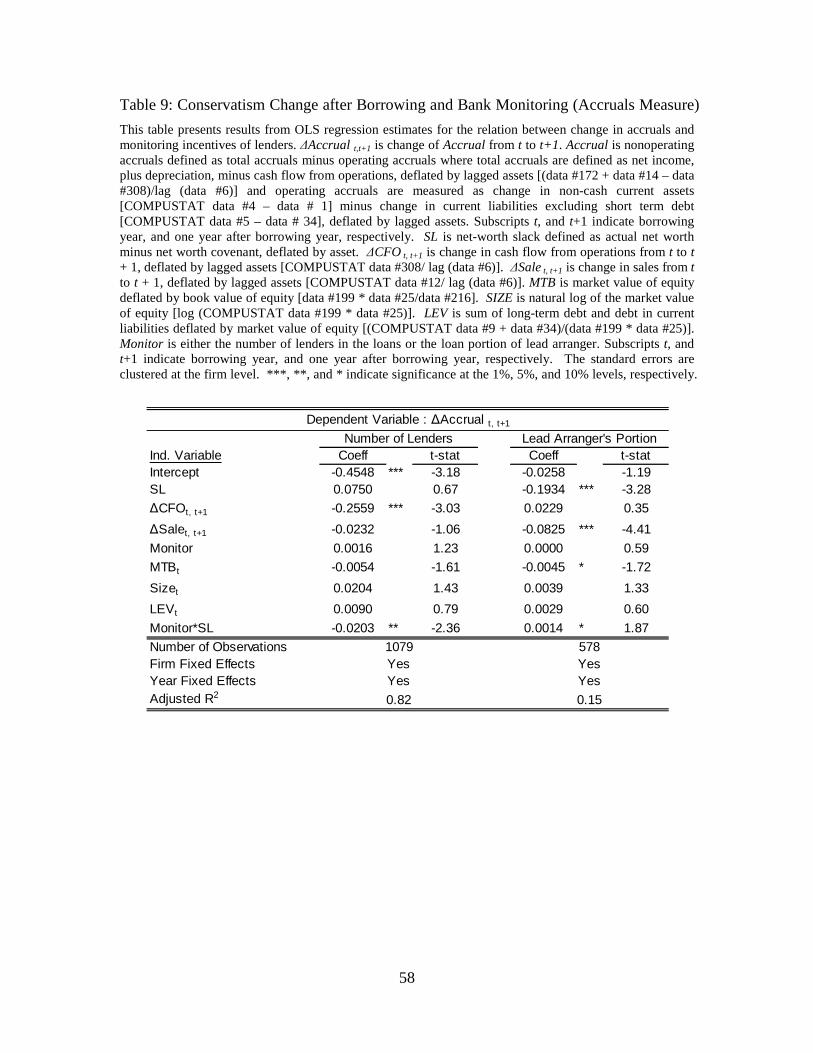
58
Table 9: Conservatism Change after Borrowing and Bank Monitoring (Accruals Measure)
This table presents results from OLS regression estimates for the relation between change in accruals and monitoring incentives of lenders. ∆Accrual t,t+1 is change of Accrual from t to t+1. Accrual is nonoperating accruals defined as total accruals minus operating accruals where total accruals are defined as net income, plus depreciation, minus cash flow from operations, deflated by lagged assets [(data #172 + data #14 – data #308)/lag (data #6)] and operating accruals are measured as change in non-cash current assets [COMPUSTAT data #4 – data # 1] minus change in current liabilities excluding short term debt [COMPUSTAT data #5 – data # 34], deflated by lagged assets. Subscripts t, and t+1 indicate borrowing year, and one year after borrowing year, respectively. SL is net-worth slack defined as actual net worth minus net worth covenant, deflated by asset. ∆CFO t, t+1 is change in cash flow from operations from t to t + 1, deflated by lagged assets [COMPUSTAT data #308/ lag (data #6)]. ∆Sale t, t+1 is change in sales from t to t + 1, deflated by lagged assets [COMPUSTAT data #12/ lag (data #6)]. MTB is market value of equity deflated by book value of equity [data #199 * data #25/data #216]. SIZE is natural log of the market value of equity [log (COMPUSTAT data #199 * data #25)]. LEV is sum of long-term debt and debt in current liabilities deflated by market value of equity [(COMPUSTAT data #9 + data #34)/(data #199 * data #25)]. Monitor is either the number of lenders in the loans or the loan portion of lead arranger. Subscripts t, and t+1 indicate borrowing year, and one year after borrowing year, respectively. The standard errors are clustered at the firm level. ***, **, and * indicate significance at the 1%, 5%, and 10% levels, respectively.
Ind. Variable Coeff t-stat Coeff t-statIntercept -0.4548 *** -3.18 -0.0258 -1.19SL 0.0750 0.67 -0.1934 *** -3.28
∆CFOt, t+1 -0.2559 *** -3.03 0.0229 0.35
∆Salet, t+1 -0.0232 -1.06 -0.0825 *** -4.41
Monitor 0.0016 1.23 0.0000 0.59
MTBt -0.0054 -1.61 -0.0045 * -1.72
Sizet 0.0204 1.43 0.0039 1.33
LEVt 0.0090 0.79 0.0029 0.60
Monitor*SL -0.0203 ** -2.36 0.0014 * 1.87
Number of ObservationsFirm Fixed EffectsYear Fixed EffectsAdjusted R2 0.82 0.15
1079 578Yes Yes
Dependent Variable : ∆Accrual t, t+1
Number of Lenders Lead Arranger's Portion
Yes Yes
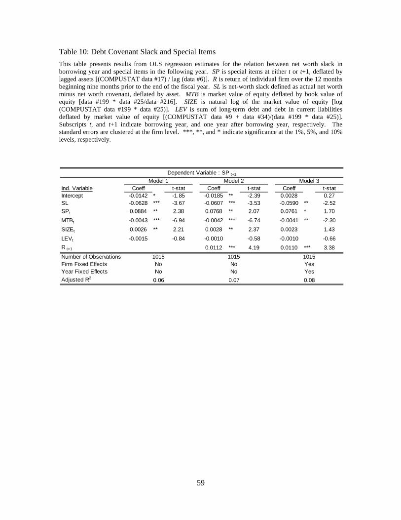
59
Table 10: Debt Covenant Slack and Special Items
This table presents results from OLS regression estimates for the relation between net worth slack in borrowing year and special items in the following year. SP is special items at either t or t+1, deflated by lagged assets [(COMPUSTAT data #17) / lag (data #6)]. R is return of individual firm over the 12 months beginning nine months prior to the end of the fiscal year. SL is net-worth slack defined as actual net worth minus net worth covenant, deflated by asset. MTB is market value of equity deflated by book value of equity [data #199 * data #25/data #216]. SIZE is natural log of the market value of equity [log (COMPUSTAT data #199 * data #25)]. LEV is sum of long-term debt and debt in current liabilities deflated by market value of equity [(COMPUSTAT data #9 + data #34)/(data #199 * data #25)]. Subscripts t, and t+1 indicate borrowing year, and one year after borrowing year, respectively. The standard errors are clustered at the firm level. ***, **, and * indicate significance at the 1%, 5%, and 10% levels, respectively.
Ind. Variable Coeff t-stat Coeff t-stat Coeff t-statIntercept -0.0142 * -1.85 -0.0185 ** -2.39 0.0028 0.27SL -0.0628 *** -3.67 -0.0607 *** -3.53 -0.0590 ** -2.52
SPt 0.0884 ** 2.38 0.0768 ** 2.07 0.0761 * 1.70
MTBt -0.0043 *** -6.94 -0.0042 *** -6.74 -0.0041 ** -2.30
SIZEt 0.0026 ** 2.21 0.0028 ** 2.37 0.0023 1.43
LEVt -0.0015 -0.84 -0.0010 -0.58 -0.0010 -0.66
R t+1 0.0112 *** 4.19 0.0110 *** 3.38
Number of ObservationsFirm Fixed EffectsYear Fixed Effects
Adjusted R2
Dependent Variable : SP t+1
Model 1 Model 2 Model 3
1015 1015 1015
0.06 0.07 0.08
No No YesNo No Yes
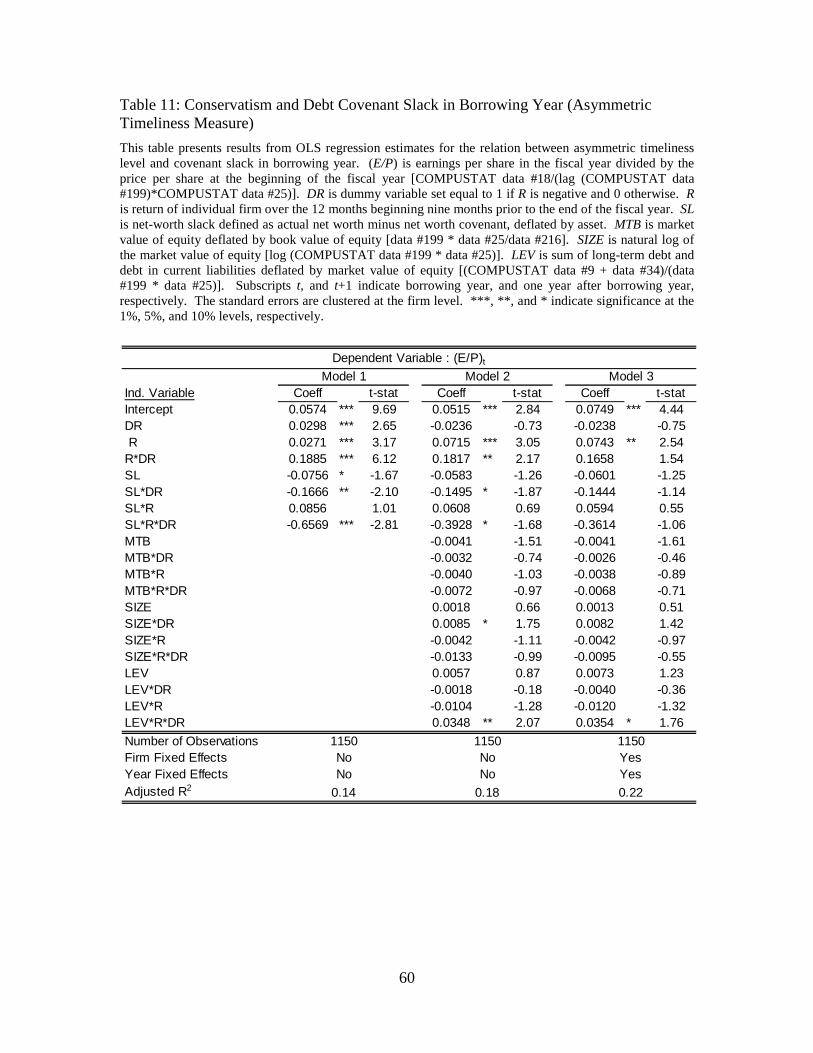
60
Table 11: Conservatism and Debt Covenant Slack in Borrowing Year (Asymmetric Timeliness Measure)
This table presents results from OLS regression estimates for the relation between asymmetric timeliness level and covenant slack in borrowing year. (E/P) is earnings per share in the fiscal year divided by the price per share at the beginning of the fiscal year [COMPUSTAT data #18/(lag (COMPUSTAT data #199)*COMPUSTAT data #25)]. DR is dummy variable set equal to 1 if R is negative and 0 otherwise. R is return of individual firm over the 12 months beginning nine months prior to the end of the fiscal year. SL is net-worth slack defined as actual net worth minus net worth covenant, deflated by asset. MTB is market value of equity deflated by book value of equity [data #199 * data #25/data #216]. SIZE is natural log of the market value of equity [log (COMPUSTAT data #199 * data #25)]. LEV is sum of long-term debt and debt in current liabilities deflated by market value of equity [(COMPUSTAT data #9 + data #34)/(data #199 * data #25)]. Subscripts t, and t+1 indicate borrowing year, and one year after borrowing year, respectively. The standard errors are clustered at the firm level. ***, **, and * indicate significance at the 1%, 5%, and 10% levels, respectively.
Ind. Variable Coeff t-stat Coeff t-stat Coeff t-statIntercept 0.0574 *** 9.69 0.0515 *** 2.84 0.0749 *** 4.44DR 0.0298 *** 2.65 -0.0236 -0.73 -0.0238 -0.75 R 0.0271 *** 3.17 0.0715 *** 3.05 0.0743 ** 2.54R*DR 0.1885 *** 6.12 0.1817 ** 2.17 0.1658 1.54SL -0.0756 * -1.67 -0.0583 -1.26 -0.0601 -1.25SL*DR -0.1666 ** -2.10 -0.1495 * -1.87 -0.1444 -1.14SL*R 0.0856 1.01 0.0608 0.69 0.0594 0.55SL*R*DR -0.6569 *** -2.81 -0.3928 * -1.68 -0.3614 -1.06MTB -0.0041 -1.51 -0.0041 -1.61MTB*DR -0.0032 -0.74 -0.0026 -0.46MTB*R -0.0040 -1.03 -0.0038 -0.89MTB*R*DR -0.0072 -0.97 -0.0068 -0.71SIZE 0.0018 0.66 0.0013 0.51SIZE*DR 0.0085 * 1.75 0.0082 1.42SIZE*R -0.0042 -1.11 -0.0042 -0.97SIZE*R*DR -0.0133 -0.99 -0.0095 -0.55LEV 0.0057 0.87 0.0073 1.23LEV*DR -0.0018 -0.18 -0.0040 -0.36LEV*R -0.0104 -1.28 -0.0120 -1.32LEV*R*DR 0.0348 ** 2.07 0.0354 * 1.76
Number of ObservationsFirm Fixed EffectsYear Fixed EffectsAdjusted R2 0.14 0.18 0.22
No No YesNo No Yes
1150 1150 1150
Dependent Variable : (E/P)t
Model 1 Model 2 Model 3
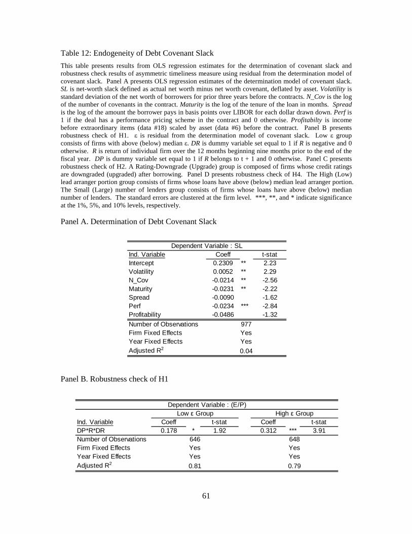
61
Table 12: Endogeneity of Debt Covenant Slack
This table presents results from OLS regression estimates for the determination of covenant slack and robustness check results of asymmetric timeliness measure using residual from the determination model of covenant slack. Panel A presents OLS regression estimates of the determination model of covenant slack. SL is net-worth slack defined as actual net worth minus net worth covenant, deflated by asset. Volatility is standard deviation of the net worth of borrowers for prior three years before the contracts. N_Cov is the log of the number of covenants in the contract. Maturity is the log of the tenure of the loan in months. Spread is the log of the amount the borrower pays in basis points over LIBOR for each dollar drawn down. Perf is 1 if the deal has a performance pricing scheme in the contract and 0 otherwise. Profitabilty is income before extraordinary items (data #18) scaled by asset (data #6) before the contract. Panel B presents robustness check of H1. ε is residual from the determination model of covenant slack. Low ε group consists of firms with above (below) median ε. DR is dummy variable set equal to 1 if R is negative and 0 otherwise. R is return of individual firm over the 12 months beginning nine months prior to the end of the fiscal year. DP is dummy variable set equal to 1 if R belongs to t + 1 and 0 otherwise. Panel C presents robustness check of H2. A Rating-Downgrade (Upgrade) group is composed of firms whose credit ratings are downgraded (upgraded) after borrowing. Panel D presents robustness check of H4. The High (Low) lead arranger portion group consists of firms whose loans have above (below) median lead arranger portion. The Small (Large) number of lenders group consists of firms whose loans have above (below) median number of lenders. The standard errors are clustered at the firm level. ***, **, and * indicate significance at the 1%, 5%, and 10% levels, respectively. Panel A. Determination of Debt Covenant Slack
Panel B. Robustness check of H1
Ind. Variable Coeff t-statIntercept 0.2309 ** 2.23Volatility 0.0052 ** 2.29N_Cov -0.0214 ** -2.56Maturity -0.0231 ** -2.22Spread -0.0090 -1.62Perf -0.0234 *** -2.84Profitability -0.0486 -1.32
Number of ObservationsFirm Fixed EffectsYear Fixed EffectsAdjusted R2
Yes
0.04
Dependent Variable : SL
977Yes
Ind. Variable Coeff t-stat Coeff t-statDP*R*DR 0.178 * 1.92 0.312 *** 3.91Number of ObservationsFirm Fixed EffectsYear Fixed EffectsAdjusted R2
YesYes
YesYes
Dependent Variable : (E/P)Low ε Group High ε Group
646 648
0.81 0.79
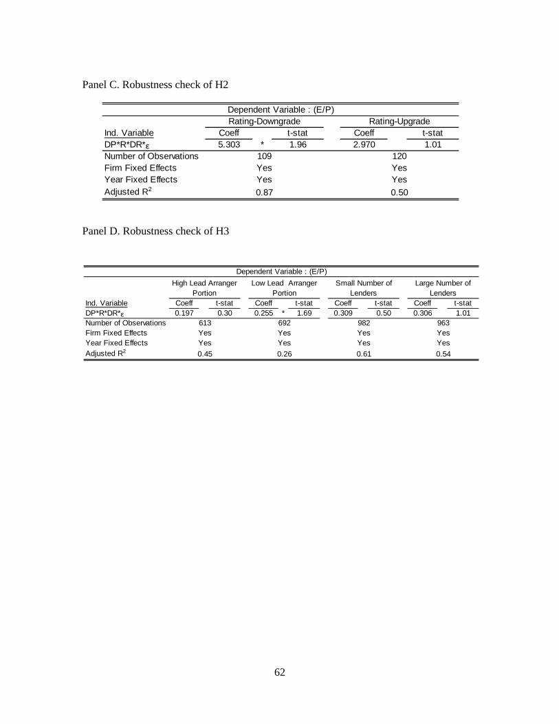
62
Panel C. Robustness check of H2
Panel D. Robustness check of H3
Ind. Variable Coeff t-stat Coeff t-statDP*R*DR*ε 5.303 * 1.96 2.970 1.01Number of ObservationsFirm Fixed EffectsYear Fixed EffectsAdjusted R2
Yes Yes
Dependent Variable : (E/P)Rating-Downgrade
0.87 0.50
Rating-Upgrade
109 120
Yes Yes
Ind. Variable Coeff t-stat Coeff t-stat Coeff t-stat Coeff t-statDP*R*DR*ε 0.197 0.30 0.255 * 1.69 0.309 0.50 0.306 1.01Number of ObservationsFirm Fixed EffectsYear Fixed EffectsAdjusted R2
Yes YesYes Yes
Yes YesYes Yes
Small Number of Lenders
Large Number of Lenders
982 963
Dependent Variable : (E/P)
0.61 0.54
High Lead Arranger Portion
Low Lead Arranger Portion
613 692
0.45 0.26
63
Chapter III
Can Firms Adjust Their Opaqueness to Lenders? Evidence from Foreign Bank Entry into India*
Todd A. Gormley1, Bong Hwan Kim2, and Xiumin Martin3
Abstract
This paper investigates the impact of financial market competition on a firm’s choice regarding accounting quality. In particular, this paper uses the entry of foreign banks into India during the 1990s—analyzing variation in both the timing of the new foreign banks’ entries and in their location—to estimate the effect of increased banking competition on firms’ timely recognition of economic losses, an important aspect of accounting quality to lenders. The estimates indicate that foreign bank entry is associated with improved accounting quality among firms, and this improvement is positively related to a firm’s subsequent debt level. The change in accounting quality appears driven by a shift in firms’ incentives to supply higher quality information to lenders and lenders seem to value this information. The increase in accounting quality is also greatest among private firms, smaller firms, less profitable firms, and firms more dependent on external financing. Overall, our evidence suggests that a firm’s opaqueness is not static, and that a firm’s choice regarding accounting quality is a function of credit market competition. Keywords: Banking Competition, Opaqueness, Accounting Quality, India JEL Classification: D82, G21, O16, M41
* Bong Hwan Kim acknowledges financial support from the Center for Research in Economics and Strategy (CRES), in the Olin Business School, Washington University in St. Louis. We also thank Rich Frankel, Radha Gopalan, Tara Rice, and seminar participants at the Financial Intermediation Research Society 2009 Annual Meeting and Washington University in St. Louis (Olin). This paper is also accepted for presentation at American Finance Association 2010 annual meeting. The Prowess data used in this paper was provided by the IMF through their visiting scholars program. The analysis and conclusions in this paper, however, are our own and do not necessarily represent those of the IMF or IMF Policy. All remaining errors and omissions are our own. 1 The Wharton School, University of Pennsylvania, 3620 Locust Walk, Suite 2400, Philadelphia, PA, 19104. Phone: (215) 746-0496. Fax: (215) 898-6200. E-mail: [email protected] 2 Olin Business School, Washington University in St. Louis, E-mail: [email protected] 3 Olin Business School, Washington University in St. Louis, Campus Box 1133, One Brookings Drive, St. Louis, MO 63130. Phone: (314) 935-6331. Fax: (314) 935-6359. E-mail: [email protected]
64
Whether increased financial market competition improves credit access for all
firms has been an open question in finance for many years. Theories that incorporate
information asymmetries demonstrate that greater competition among lenders has the
potential to reduce credit access for informationally-opaque firms (Petersen and Rajan,
1995), and evidence from the deregulation of U.S. banking markets seems to support this
possibility (Zarutskie, 2006). The welfare of such opaque firms in competitive lending
environments, however, may depend on a number of factors. The source of competition
(Boot and Thakor, 2000) and the response of existing lenders to increased competition
(Dell’Ariccia and Marquez, 2004; Sengupta, 2007) may each affect whether opaque firms
are adversely affected by an increase in financial competition.
Another, less explored, factor that might affect the impact of increased financial
competition on opaque firms is the extent to which firms’ opaqueness is fixed. By
providing lenders with higher quality financial reports, firms can reduce their opaqueness
when the cost of being opaque increases. One way firms could accomplish this is
through a more timely accounting recognition of economic losses. While timely loss
recognition can be costly for firms by lowering stated earnings, which may then reduce
outsiders’ valuation of the company and constrain dividend payments, it can benefit firms
by enhancing the efficiency of debt contracting and improving a firm’s ability to obtain
debt-financing (Ahmed, Billings, Morton, and Harris, 2002; Ball and Shivakumar, 2005;
Leuz, Nanda and Wysocki, 2003).4 This enhanced efficiency occurs because timely loss
recognition, which is easily verified by a lender using a firm’s historic accounting
statements, reduces the likelihood of a borrower’s current financial position being
4 The costs and benefits of timely loss recognition have been extensively studied in the accounting literature. For more details, see Watts and Zimmerman (1990) and Watts (2003a).

65
overstated. This enables lenders to better screen borrowers’ creditworthiness, to
construct financial covenants more effectively, and to mitigate agency conflicts
pertaining to dividend policy.
The possibility that a firm’s opaqueness may not be static is the focus of our paper.
In particular, we ask the following questions: Does a firm’s accounting quality change
when credit market competition and the cost of being opaque increases? And if so, for
which firms are these changes most prominent, and do lenders appear to value these
changes? To answer these questions, we study firms’ accounting choices during the entry
of foreign banks into India in the 1990s.
The entry of foreign banks into India provides two key advantages in analyzing
whether firms adjust their accounting quality to reflect changes in lending environments.
First, theory suggests that the costs of being opaque may be particularly high following
an increase in financial competition. Foreign bank’s entry into India leads to an increase
in financial competition, which may directly increase the cost of being opaque (Petersen
and Rajan, 1995). Additionally, foreign banks may also be less able to acquire soft
information about local firms (Stein, 2002). This limited information may lead foreign
banks to only finance firms that are less informationally opaque, larger, or extremely
profitable (Dell’Arricia and Marquez, 2004; Segupta, 2007), and this ‘cream-skimming’
by foreign banks can reduce opaque firms’ access to domestic lenders (Detragiache,
Gupta, and Tressal, 2008; Gormley, 2007).
Second, geographical variation in foreign bank locations over time facilitates the
use of novel identification techniques. We make use of the staggered entry of foreign
banks into India following the country’s 1994 commitment to the World Trade

66
Organization (WTO). Some districts of India received a foreign bank branch as early as
1994, while others did not receive such a branch until 2001, and as of today, many
districts have yet to receive a foreign bank. Matching this information to a large panel
dataset of firms’ audited financial statements, we compare changes in accounting quality
between domestic firms located geographically near the new foreign banks and domestic
firms located further from the new foreign banks. The variation both in the timing of the
new foreign banks’ entries and in their location within the country reduces potential
confounding effects that might arise from other country-wide changes in financial market
competitiveness or accounting standards. Such country-wide changes would affect all
firms in India and therefore unlikely explain differential changes in accounting quality for
firms located geographically near foreign banks versus those that are not. By using firm-
level data, we can also test for heterogeneous effect across firms as well as control for
any differences in the types of firms located in areas with a new foreign bank.
To measure a firms’ timely recognition of economic losses, we rely on established
methodologies in the accounting literature. In particular, we follow the research design
by Ball and Shivakumar (2005) and apply an accrual-cash flow non-linear regression
technique. Since this measure of accounting timeliness only relies on the information in
firms’ historical financial statements, we are able to calculate it for both public and
private firms in India. This is particularly important since the cost of being opaque is
likely more acute for private firms after foreign bank entry. Following Basu (1997), we
also adopt another measure of timely loss recognition using earnings time-series
regression, and our main results are robust to this alternative measure.
Using the aforementioned framework, we find evidence that firms’ accounting

67
choices are associated with changes in the lending environment. The overall level of
accounting quality, as measured by the timely loss recognition, increases for firms
located in the vicinity of new foreign banks following their entry. Firms located in
districts without any foreign bank entry do not change their financial reporting policies,
and there is no evidence of timely loss recognition prior to foreign bank entry. The
increases in accounting quality are concentrated among firms with the strongest
incentives to adjust their accounting procedures so as to reduce information asymmetries
and alleviate financing constraints. We find that smaller, less profitable, and private firms,
particularly private firms with greater dependence on external financing, increase their
timely loss recognition the most. The findings are robust to the use of different samples,
control variables, and model specifications.
The evidence also indicates that lenders value this change in accounting quality.
Within districts that experience a foreign bank entry, we find the largest accounting
quality improvements occur, on average, among firms that maintain or increase their
level of borrowings following foreign bank entry, whereas firms that experience declines
in their debt levels exhibit a smaller average increase in accounting quality.
The evidence in this study provides a new perspective to the potential effects of
greater financial market competition on lending relationships and the supply of credit to
informationally-opaque firms (Berger, Saunders, Scalise, and Udell, 1998; Degryse and
Ongena, 2007; Sapienza, 2002; Rice and Strahan, 2009; and Zarutskie, 2006). Contrary
to analyzing whether the credit access or performance of opaque firms decline, our paper
looks at whether these firms reduce their opaqueness to lenders following an increase in
financial competition. Our evidence suggests that firms’ opaqueness may not be
68
completely fixed and that firms attempt to furnish additional and easily verifiable
information to lenders to mitigate the potential adverse outcomes of greater financial
market competition. This possible adjustment by firms has been overlooked in the
existing literature that studies the potential effects of greater bank competition.
This paper is also related to the empirical literature that studies the relationships
between foreign bank entry, domestic bank performance, interest rates, and firms’ debt
usage.5 This paper compliments this literature by analyzing the changes in firms’
accounting practices following foreign bank entry and showing that these changes may be
related to a firm’s demand for credit. In the extant literature, there is a void in
investigating how firms adapt their behavior in response to foreign lenders’ entry, with
the exception of Berger, Klapper, Peria, and Zaidi (2008). They document that firms may
choose to have multiple bank relationships as an insurance against the ‘fragility’ of
foreign bank relationships. Our study provides evidence that domestic firms may also
resort to improving accounting quality to alleviate information asymmetries and the
potential adverse effects of foreign bank entry. The observed increase is consistent with
theories suggesting that competition from foreign lenders may affect the importance of
firms’ opaqueness (Dell’Arricia and Marquez, 2004; Gormley, 2007; Sengupta, 2007).
Finally, our paper is related to the accounting literature that analyzes the
importance of timely loss recognition and its impact on debt contracts (Ahmed, Billings,
Morton, and Harris, 2002; Zhang, 2008; Moerman, 2008; Beatty, Weber, and Yu, 2008;
5 Claessens, Demirguc-Kunt, and Huizinga (2001) uncover evidence that foreign bank entry is associated with lower profit margins among domestic banks, while Berger, Klapper, and Udell (2001), Haber and Musacchio (2004), and Mian (2006) provide evidence that foreign banks tend to finance only larger, more established firms. Clarke, Cull, and Martinez Peria (2006) find that entrepreneurs in countries with high levels of foreign bank ownership perceive interest rates and access to loans as smaller constraints to their operations. Detragiache, Gupta, and Tressal (2008) and Gormley (2008) find that foreign ownership is negatively related to aggregate and firm-level measures of debt-usage, while within Eastern European countries, Giannetti and Ongena (2009a) find the share of foreign lending to be positively related to firm-level sales and overall debt usage, particularly for larger firms. Giannetti and Ongena (2009b) also find that foreign bank entry may make bank relationships more stable and enhance financial access.

69
Guay 2008). Rather than analyze the importance of timely reporting of losses in a static
credit market, however, our paper tests whether changes in lending market competition
are correlated to changes in firms’ accounting choices.6 Our paper provides supporting
evidence to the arguments of Ball (2001) and Kothari (2001) that institutional
mechanisms are important in shaping a country’s accounting quality. Our paper also
corroborates Ball, Robin, and Sadka (2008), who show that the debt market rather than
the equity market drives timely loss recognition among firms.
The remainder of the paper proceeds as follows. Section 1 provides a review of
India’s policy change. Section 2 develops testable hypotheses. Section 3 describes the
data and research design. Section 4 presents empirical results, and Section 5 concludes.
1. Description of Policy Change in India
Prior to 1991, India’s economy and financial system was heavily regulated and
dominated by the public sector. Following a balance of payments crisis in 1991, however,
a number of structural reforms were implemented that greatly deregulated many
economic activities. In November 1991, a broad financial reform agenda was established
in India by the Committee on the Financial System (CFS). One of the committee’s
recommendations to meet this goal was to introduce greater competition into the banking
system by allowing more foreign banks to enter India.
However, no significant action was taken by the Government of India regarding
the CFS recommendation on foreign banks until April 1994 when the government agreed
to allow for an expansion of foreign banks under the General Agreement on Trades in
Services (GATS). In the initial GATS agreement, India committed to issue five additional
branch licenses to both new and existing foreign banks each year. In a subsequent
6 One exception to the completely static analysis is Ball, Kothari, and Ashok (2000), which examines differences in firms’ timely loss recognition using cross-country variation in debt market development.

70
supplemental agreement in July 1995, India increased the limit to eight licenses per year,
and in February 1998, the limit was increased to 12. While there were no restrictions on
where foreign banks could choose to establish new branches, the expansion of foreign
banks in India was allowed by de novo branches only.7
In the years preceding the signing of the GATS agreement, very few licenses for
new foreign bank branches were granted, and the presence of foreign banks in India was
limited. On March 31, 1994 there were 24 foreign banks with 156 branches in India.
Most of these banks, however, had begun operations before India’s first nationalization of
private banks in April 1969, and only seven new branches had opened since 1990.
Moreover, most of India’s 575 districts did not have a foreign bank, as roughly 75
percent of these foreign bank branches were concentrated in districts encompassing
India’s three largest cities: Delhi, Mumbai, and Kolkata.
In the eight years following the acceptance of GATS, however, 17 new foreign
banks and 89 new foreign bank branches were opened in India bringing the total number
foreign banks to 41 with 212 branches as of March 2002.8 The expansion of foreign
banks also increased their representation outside of India’s most populous cities, as the
number of districts with a foreign bank increased from 18 to 26, and foreign banks’ share
of total long-term loans increased as well. In March 1994, foreign banks accounted for 5
percent of all outstanding long-term loans, but with their expansion of branches, their
share of long-term loans increased and averaged roughly 8 percent from 1996 to 1998,
7 Foreign banks were not allowed to own controlling stakes in domestic banks, and foreign banks wishing to establish new branches needed to seek Reserve Bank of India approval, as do all banks under Section 23 of the Banking Regulation Act, 1949. Requests for new branches are evaluated on the “merits of each case and taking into consideration overall financial position of the bank, quality of its management, efficacy of the internal control system, profitability, and other relevant factors”. See “Master Circular on Branch Licensing,” DBOD.No. BL.BC. 5/22.01.001/2004, Reserve Bank of India, Mumbai, pp. 4. 8 33 foreign bank branches closed during this time period, so the net change was only 56. 17 of these closures were from ANZ Grindlays Bank Ltd. and five from Standard Chartered Bank in 1998 and 1999.

71
and 10 percent from 1999 to 2001. Moreover, some back of the envelope calculations
suggest foreign bank entry was sizeable in the eight districts receiving their first foreign
bank. By 2003, foreign banks accounted for roughly 5.5 percent of long-term loans in
these districts, and their share of loans is about 10 percent in districts that experienced
entry between 1994 and 1996, suggesting foreign banks’ share of loans grows with time.
The entry of foreign banks into India appears to have reduced credit access for
opaque firms. Gormley (2008) finds that while average bank borrowings increased for
large, profitable firms following foreign bank entry into India, the average domestic firm
located in the vicinity of a new foreign bank experienced a drop in bank borrowings.
These declines were larger on average among firms generally considered more opaque,
such as smaller firms and firms with fewer tangible assets. The drop in credit also
appears to adversely affect the performance of smaller firms with greater dependence on
external financing. The experience of India is consistent with the cross-country evidence
of Detragiache, Gupta, and Tressal (2008), which also finds evidence that foreign bank
entry is associated with reduced bank credit among opaque firms.
The reduced use of debt for many opaque firms in India would seem to suggest
that the cost of being opaque increased following foreign bank entry. We now turn to
exploring why this might occur and how firms might be expected to respond.
2. Hypotheses Development
In making lending decisions, banks face ex-ante information asymmetry and ex-
post moral hazard problems. To overcome these frictions, banks can adopt stringent
screening standards (Ramakrishnan and Thakor, 1984) and/or monitor borrowers
(Diamond, 1984). Each requires information about the creditworthiness of borrowers.
While some information on credit quality can be obtained from credit agencies, suppliers,
72
and customers of a firm, a large share of the information used by lenders will be
contained in the firms’ financial statements. The quality of these financial statements
will hence affect lending decisions.
One particular accounting quality that may affect lending decisions is the timely
accounting recognition of economic losses (Watts and Zimmerman, 1986; Ahmed,
Billings, Morton, and Harris, 2002; Watts, 2003a, 2003b; Beatty, Weber, and Yu, 2008).9
Because of lenders’ asymmetric payoff from firms’ net assets (lenders incur loss when
the net assets of borrower are below the principal but are not compensated when net
assets exceed the principal), lenders are concerned with the lower bound of a borrower’s
net asset value. Timely loss recognition ensures, however, that expected losses are
reflected in the financial statements earlier and that the borrowers’ true net asset value is
not overstated (Watts, 2003a). This lower bound is informative to the lenders in making
lending decisions and in specifying financial covenants.10 Timely loss recognition also
increases the effectiveness of ex-post monitoring because it better informs lenders about a
borrower’s ability to repay, and the decreased reported earnings help constrain dividends,
thus alleviating the ex-post moral hazard problems (Watts and Zimmerman, 1986).
Several studies find evidence consistent with timely loss recognition having a
positive effect on lending decisions. Ahmed, Billings, Morton, and Harris (2002) find
evidence that timely loss recognition plays an important role in mitigating bondholder
and shareholder conflicts over dividend policy and in reducing firms’ borrowing costs.
9 More specifically, timely accounting recognition of economic losses is also termed as asymmetric timeliness or conditional conservatism. Ball and Shivakumar (2005, pp. 88-92) explain the role of conditional conservatism in efficient contracting, and contrast it with unconditional conservatism which is argued to have no positive effect on efficient contracting. 10 There is evidence that banks in India use covenants to monitor borrowers. For example, on February 11, 2001, the Financial Times reported that Indian banks “have been asked by the Reserve Bank of India to make bill finance one of the covenants for sanction of working capital credit limits”.
73
Zhang (2008) shows that timely loss recognition benefits lenders through a timely
signaling of default risk, and in return, benefits borrowers through a lower cost of debt.
Beatty, Weber and Yu (2008) find evidence that debt covenants and conservative
financial reports are complementary in meeting lenders’ demand.
On the other hand, timely loss recognition can be costly for firms. Earlier
recognition of losses lowers stated earnings, which may reduce outsiders’ valuation of the
company and constrain dividend payment to shareholders (Ahmed, Billings, Morton, and
Harris, 2002). Firms also violate debt covenants earlier when they are timely in
recognition of losses (Zhang, 2008), and such violations can be costly for firms (Roberts
and Sufi, 2009). Timely loss recognition may also reduce a manager’s private benefits,
particularly in countries with weak investor protections (Leuz, Nanda and Wysocki,
2003).
Given these costs, firms face a trade-off when choosing how timely to recognize
economic losses. Holding all else equal, loss recognition is expected to be more timely
when the potential benefits of doing so increase, and vice versa, loss recognition should
be less timely when the potential costs increase.
By increasing both the cost of being opaque and the reliance on ‘hard’
information in making lending decisions, the entry of foreign banks is likely to affect this
tradeoff in increasing the benefits of timely loss recognition. First, foreign bank entry
will increase banking competition, which has the potential to reduce credit access for
opaque firms (Petersen and Rajan, 1995). Second, foreign banks’ higher cost of
acquiring information about local firms (Berger, Klapper, and Udell, 2001; Stein, 2002;
Mian, 2006) may limit their willingness to finance opaque, smaller, or less profitable

74
firms (Dell’Arricia and Marquez, 2004; Segupta, 2007; Gormley, 2007). Third, foreign
banks’ use of largely arm-length transactions that rely more heavily on hard information
will increase the importance of a firm’s accounting quality in making lending decisions.
Domestic lenders may also adopt these ‘best practices’ of foreign banks, further
increasing the importance of a firm’s accounting quality in the lending process (Lensink
and Hermes, 2004).
The increased cost of being opaque and potential change in lenders’ demand for
accounting quality following foreign bank entry provides firms with an incentive to
reduce their opaqueness to lenders. Since timely loss recognition may help accomplish
this, we conjecture it will increase after foreign bank entry. Therefore, our first
hypothesis is stated as follows:
HYPOTHESIS 1 (H1): The level of timely loss recognition will increase in districts
where foreign bank entry occurs.
A rejection of this hypothesis would indicate that foreign bank entry has no
impact on timely loss recognition. This might occur if lending competition, as captured
by foreign bank entry, does not increase the cost of being opaque, or if lenders do not
value this particular change in accounting quality.
The increased cost of being opaque following foreign bank entry is also likely to
vary across firms. More opaque firms will be at a larger disadvantage if lenders place
greater emphasis on hard information when making lending decisions. Additionally,
firms that are more dependent on external financing may find it more beneficial to
increase accounting quality if doing so can increase the odds of maintaining credit access.
As a result, small and private firms, which are typically more informationally-opaque and

75
dependent on external financing, may have the greatest incentive to adjust accounting
quality `following foreign bank entry. Less profitable firms may also have a greater
incentive to improve their accounting quality. Bernanke and Gertler (1989) argue that
less profitable firms may have greater agency costs of debt arising from information
asymmetries between lenders and borrowers. Our second hypothesis is stated as follows:
HYPOTHESIS 2 (H2): The change in timely loss recognition will be more
pronounced among less profitable, small and private firms, and firms with
greater external financing dependence.
Finally, if increased timely loss recognition reduces firms’ opaqueness and the
risk born by lenders in assessing firms’ creditworthiness, we expect lenders to reward
firms who increase the supply of accounting quality by granting more credit to these
firms. Therefore, our third hypothesis is stated as follows:
HYPOTHESIS 3 (H3): The change in timely loss recognition after foreign bank
entry will be positively associated with firms’ access to credit.
3. Data and Research Design
3.1. Data
The data used to identify the location and opening date for each foreign bank in
India is the Directory of Bank Offices published by the Reserve Bank of India. Providing
the location, name, opening date, and closing date for every bank office in India, the data
is used to construct a complete annual directory of all banks in India from 1988 to 2004.
With this data, it is possible to map out the timing and location of arrival for the
new foreign banks. Table 1 shows the number of foreign banks by district and year from
1990 to 2002. In the top half of the table are the 18 districts that already had a foreign
bank before 1991. These include the three districts with very large metropolitan centers:

76
Delhi, Greater Mumbai, and Kolkata. In the bottom half are the eight districts that
received their first foreign bank during the 1990s. As can be quickly seen, the overall
increase in foreign bank branches largely coincides with the signing of the GATS in 1994,
but the actual timing of entry across these eight districts is staggered across years. The
district location of new foreign banks is mapped in Figure 1 which highlights the eight
districts that receive their first foreign bank between 1991 and 2002. The eight districts
are relatively dispersed across India, spanning seven of India’s 35 states.11
[Insert Table 1 here]
[Insert Figure 1 here]
The bank location data are matched up to the Prowess data set compiled by the
Centre for Monitoring Indian Economy (CMIE). Prowess is a panel data set of firms
from 1988 to 2002 where both listed and unlisted publicly limited Indian and foreign
firms with assets plus sales greater than 40 million Rupees (approx. $900,000) are
included in the data set.12 The data set provides the annual financial and accounting data
of each firm along with descriptive variables including the ownership, year of
incorporation, and registered address. Using each firm’s address, it is possible to track
their financial status at the district level and to merge this data to the district location of
the new foreign banks in India. We exclude firm-year observations for firms located in
the districts that already have foreign banks prior to 1991 because these banks are usually
located in the big metropolitan areas and firms in these areas are different in many ways,
11 Citibank and Hong Kong & Shanghai Banking (HSBC) were responsible for half of the new foreign bank branches in the eight districts. Other banks opening branches in these districts were ABN AMRO, American Express Bank Ltd., ANZ Grindlays, BNP Paribas, Crédit Lyonnais, Deutsche Bank (Asia), Société Générale, and Standard Chartered. Each had pre-existing branches elsewhere in India at the time of entry in the eight districts. 12 CMIE compiles the financial data using the audited annual accounts that all registered companies in India must submit to the Registrar of Companies. The cutoff level of firm size in the Prowess dataset seems to be an arbitrary point chosen to limit the size of the database.

77
which can be seen in Appendix Table 1.13 Because of fewer data points and the heavy
regulation of the Indian banking system and economy prior to 1992, we also exclude
observations prior to 1992 from our main analysis. Our final sample consists of 20,438
firm-year observations for 2,547 unique firms over the period 1992-2002.
While foreign banks only entered eight new Indian districts after 1992, the
financial data provided by Prowess indicates that a large number of Indian firms were
likely affected by this entry. Within our sample, these eight districts account for 25
percent of the observed firms and 24 percent of total sales in 1992. These high numbers
reflect foreign banks’ tendency to locate in heavily populated districts.
3.2. Measuring timely loss recognition
3.2.1. Accruals-cash flows model
Following Ball and Shivakumar (2005), we measure timely loss recognition using
a non-linear relation between operating cash flows and accruals. The model is as follows:
1 2 3it it it it it itACC DCFO CFO DCFO CFOβ β β ε= + + × + (1)
The dependent variable ACCit is accruals computed as [(∆CAit – ∆Cashit ) –
(∆CLit - ∆STDit ) – DEPit ] scaled by total assets for firm i in year t, where ∆CA is the
change in current assets, ∆Cash is the change in cash and bank balances, ∆CL is the
change in current liabilities, ∆STD is the change in short term debt, and DEP is
depreciation expense. CFO represents the operating cash flows (scaled by total assets),
measured as the difference between ROA and ACC , where ROA is the profit after tax
13 Comparing the summary statistics in the appendix with those in Table 2 suggests that firms located in the areas with foreign banks entry prior to 1991 are much larger in size than firms in our sample. They are also more profitable as measured by their return on assets (ROA), and have higher cash flow from operations.
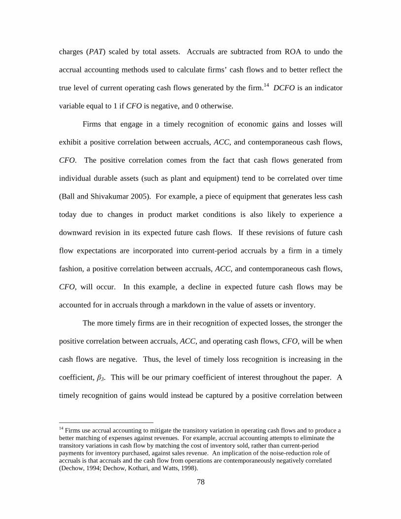
78
charges (PAT) scaled by total assets. Accruals are subtracted from ROA to undo the
accrual accounting methods used to calculate firms’ cash flows and to better reflect the
true level of current operating cash flows generated by the firm.14 DCFO is an indicator
variable equal to 1 if CFO is negative, and 0 otherwise.
Firms that engage in a timely recognition of economic gains and losses will
exhibit a positive correlation between accruals, ACC, and contemporaneous cash flows,
CFO. The positive correlation comes from the fact that cash flows generated from
individual durable assets (such as plant and equipment) tend to be correlated over time
(Ball and Shivakumar 2005). For example, a piece of equipment that generates less cash
today due to changes in product market conditions is also likely to experience a
downward revision in its expected future cash flows. If these revisions of future cash
flow expectations are incorporated into current-period accruals by a firm in a timely
fashion, a positive correlation between accruals, ACC, and contemporaneous cash flows,
CFO, will occur. In this example, a decline in expected future cash flows may be
accounted for in accruals through a markdown in the value of assets or inventory.
The more timely firms are in their recognition of expected losses, the stronger the
positive correlation between accruals, ACC, and operating cash flows, CFO, will be when
cash flows are negative. Thus, the level of timely loss recognition is increasing in the
coefficient, β3. This will be our primary coefficient of interest throughout the paper. A
timely recognition of gains would instead be captured by a positive correlation between
14 Firms use accrual accounting to mitigate the transitory variation in operating cash flows and to produce a better matching of expenses against revenues. For example, accrual accounting attempts to eliminate the transitory variations in cash flow by matching the cost of inventory sold, rather than current-period payments for inventory purchased, against sales revenue. An implication of the noise-reduction role of accruals is that accruals and the cash flow from operations are contemporaneously negatively correlated (Dechow, 1994; Dechow, Kothari, and Watts, 1998).

79
cash flows and accruals when current cash flows are positive (i.e. β2>0). However,
because standard accounting practices generally do not allow firms to account for
expected future gains in cash flows until those gains are actually realized, there is little
positive correlation between positive cash flows and accruals on average. This
asymmetry in the correlation between accruals and cash flows is why ‘timely loss
recognition' is often referred to as ‘asymmetric timeliness’.
3.2.2 Basu’s (1997) earnings time-series model
To corroborate results based on accruals-cash flow measure of timely loss
recognition, we also use the Basu’s (1997) earnings time-series model as another measure.
The model specification is as follows:
1 1 2 1 3 1 1β β β ε− − − −∆ = + ∆ + ∆ × +it it it it it itNI D NI NI D (2)
In model (2), the dependent variable ∆NIt is the change in ROA from fiscal year t-
1 to t. The explanatory variable Dit-1 is a dummy equal to 1 if ∆NIt-1 is negative, and 0
otherwise. To the extent that the recognition of expected economic gains is subject to
realization requirements, a positive shock to earnings will only be gradually incorporated
into a firm’s earnings over time. This will imply that an increase in earnings this period
will have persistence and a positive ∆NIt-1 will be associated with a positive ∆NIt (i.e.,
2 0β > ). If firms recognize economic losses on a timelier basis than economic gains,
then a negative shock to expected earnings is recognized immediately and fully rather
than waiting for actual realization. Therefore, timely loss recognition implies a decrease
in earnings this period is likely to be transitory. This asymmetry in the persistence of
earning changes predicts3β (which captures the incremental timeliness in the recognition

80
of economic losses) to be negative, (i.e.,3 0β < ).
3.3 Research design
3.3.1. Regression using accruals and cash flows model
To test whether foreign bank entry is correlated with timely loss recognition, we
expand model (1) by introducing a dummy variable, Bank, to capture foreign bank entry,
and interact it with other explanatory variables in model (1). In particular, the model we
estimate is specified as follows:
1 2 3
4 5 6
7
idt idt idt idt idt
dt dt idt dt idt
dt idt idt i t it
ACC DCFO CFO DCFO CFO
Bank Bank DCFO Bank CFO
Bank DCFO CFO
β β β
β β β
β α δ ε
= + + ×
+ + × + ×
× × + + +
(3)
where Bankdt is equal to 1 if a foreign bank is present in district d in year t , and 0
otherwise. The regression also includes firm fixed effects, αi , to control for time-
invariant differences across firms, and year fixed effect, δ t , to control for non-secular
time trends in average accounting quality across India. Since foreign entry occurs at the
district level, standard errors are clustered at the district-level.
By interacting Bankdt with the main specification of Ball and Shivakumar (2005)
and including year and firm fixed effects, this new specification will make use of
variation both in the location and timing of foreign bank entry to identify the impact of
foreign bank entry on timely loss recognition. The main coefficient of interest, β7, will
test the changes in timely loss recognition for firms located in a district with a new
foreign bank after its entry relative to changes for firms located elsewhere in India. A
positive β7 would support Hypothesis 1 (H1) and indicate that timely loss recognition
increased for firms located near a new foreign bank after entry relative to other firms

81
located elsewhere in India.
The use of variation in both the location and timing of foreign bank entry reduces
potential confounding effects that might arise from country-wide changes in accounting
quality or fixed differences in accounting quality across firms. Changes in average
accounting quality over time, which might arise from other country-level reforms or
changes in financial competitiveness, would be absorbed by the year dummies. Likewise,
fixed differences in average accounting quality or the opaqueness of firms located in
districts experiencing entry will be captured by the firm-level fixed effects.
This difference-in-difference estimation relies on two identification assumptions.
First, it implicitly assumes that the effect of foreign bank entry is localized and realized
predominately by firms headquartered in the district with a foreign bank. In general, we
expect this to hold as empirical work in other countries has demonstrated the average
distance between firms and their bank is usually quite small.15 However, even if this
assumption is not fully true, this would only bias the results against finding an effect of
foreign bank entry on accounting quality because some firms affected by foreign bank
entry would be wrongly classified as control firms in the estimation.16
The second identification assumption is that foreign banks did not select into
districts that were already trending differently or going to trend differently in the future,
15 Analyzing small firms in the U.S., Petersen and Rajan (2002) finds that the average distance between a firm and its main bank was 67.8 miles in 1993, and the median distance was five miles. The Indian districts included in this sample had an average size of 2,457 square miles. While the U.S. firms sampled were on average six times smaller than the firms found in the Prowess data, it is likely the Indian firms also borrow locally as the positive relation between distance and borrowing costs are likely greater in a developing country such as India. Recent work on lending relationships and loan prices in Belgium and the U.S. also suggest that greater lending distances are associated with increased transportation and informational costs (Agarwal and Hauswald, 2007; Degryse and Ongena, 2005). 16 As a robustness check, we also examine the relation between foreign bank entry and timely loss recognition for firms located in the neighborhood of the districts with foreign bank entry. Results suggest that timely loss recognition does not change for these firms after foreign bank entry, which lends empirical support to our identification assumption.
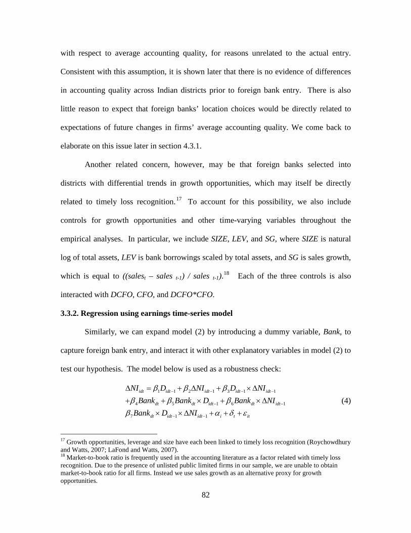
82
with respect to average accounting quality, for reasons unrelated to the actual entry.
Consistent with this assumption, it is shown later that there is no evidence of differences
in accounting quality across Indian districts prior to foreign bank entry. There is also
little reason to expect that foreign banks’ location choices would be directly related to
expectations of future changes in firms’ average accounting quality. We come back to
elaborate on this issue later in section 4.3.1.
Another related concern, however, may be that foreign banks selected into
districts with differential trends in growth opportunities, which may itself be directly
related to timely loss recognition.17 To account for this possibility, we also include
controls for growth opportunities and other time-varying variables throughout the
empirical analyses. In particular, we include SIZE, LEV, and SG, where SIZE is natural
log of total assets, LEV is bank borrowings scaled by total assets, and SG is sales growth,
which is equal to ((salest – sales t-1) / sales t-1).18 Each of the three controls is also
interacted with DCFO, CFO, and DCFO*CFO.
3.3.2. Regression using earnings time-series model
Similarly, we can expand model (2) by introducing a dummy variable, Bank, to
capture foreign bank entry, and interact it with other explanatory variables in model (2) to
test our hypothesis. The model below is used as a robustness check:
1 1 2 1 3 1 1
4 5 1 6 1
7 1 1
idt idt idt idt idt
dt dt idt dt idt
dt idt idt i t it
NI D NI D NI
Bank Bank D Bank NI
Bank D NI
β β β
β β β
β α δ ε
− − − −
− −
− −
∆ = + ∆ + ×∆
+ + × + ×∆
× ×∆ + + +
(4)
17 Growth opportunities, leverage and size have each been linked to timely loss recognition (Roychowdhury and Watts, 2007; LaFond and Watts, 2007). 18 Market-to-book ratio is frequently used in the accounting literature as a factor related with timely loss recognition. Due to the presence of unlisted public limited firms in our sample, we are unable to obtain market-to-book ratio for all firms. Instead we use sales growth as an alternative proxy for growth opportunities.

83
All variables are as defined previously. The regression also includes firm fixed effects,
αi , to control for time-invariant differences across firms, and year fixed effect, δ t , to
control for non-secular time trends in accounting practice across India. Since foreign
entry occurs at the district level, standard errors are clustered at the district-level. Based
on H1, we expect the coefficient, β7 , to be negative. This would indicate that timely loss
recognition increases for firms located near a new foreign bank after its entry relative to
other firms located elsewhere in India.
4. Empirical Results
4.1. Descriptive statistics
Table 2 reports descriptive statistics for our sample of firms. The average total
assets of firms in our sample is 2.5 billion Rupee (approximately $60 million) and the
median is 320 million Rp (approximately $7.4 million). ROA (net income/assets) has a
mean of -0.4 percent and a median of 1.2 percent, suggesting that on average, Indian
firms incur losses. Accruals has a mean of -0.005, indicating that accruals decrease
income on average in India, and cash flows has a mean of 0.
Profitability and cash flows of firms in districts where foreign bank entry occurs
are similar to the profitability and cash flows of firms in districts with no foreign bank
entry. Panel B presents separately the summary statistics for firms located in the districts
with foreign bank entry (N=3,450), and Panel C presents summary statistics for firms
located in districts with no foreign bank entry (N=16,988). On average, firms located in
districts with foreign bank entry are slightly less profitable, and have lower accruals and
cash flows compared to firms located in districts where foreign bank entry does not occur,
but the differences are small and not statistically different.
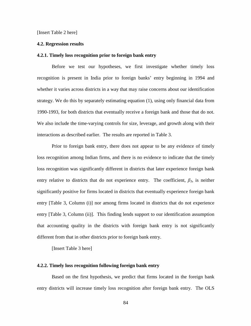
84
[Insert Table 2 here]
4.2. Regression results
4.2.1. Timely loss recognition prior to foreign bank entry
Before we test our hypotheses, we first investigate whether timely loss
recognition is present in India prior to foreign banks’ entry beginning in 1994 and
whether it varies across districts in a way that may raise concerns about our identification
strategy. We do this by separately estimating equation (1), using only financial data from
1990-1993, for both districts that eventually receive a foreign bank and those that do not.
We also include the time-varying controls for size, leverage, and growth along with their
interactions as described earlier. The results are reported in Table 3.
Prior to foreign bank entry, there does not appear to be any evidence of timely
loss recognition among Indian firms, and there is no evidence to indicate that the timely
loss recognition was significantly different in districts that later experience foreign bank
entry relative to districts that do not experience entry. The coefficient, β3, is neither
significantly positive for firms located in districts that eventually experience foreign bank
entry [Table 3, Column (i)] nor among firms located in districts that do not experience
entry [Table 3, Column (ii)]. This finding lends support to our identification assumption
that accounting quality in the districts with foreign bank entry is not significantly
different from that in other districts prior to foreign bank entry.
[Insert Table 3 here]
4.2.2. Timely loss recognition following foreign bank entry
Based on the first hypothesis, we predict that firms located in the foreign bank
entry districts will increase timely loss recognition after foreign bank entry. The OLS
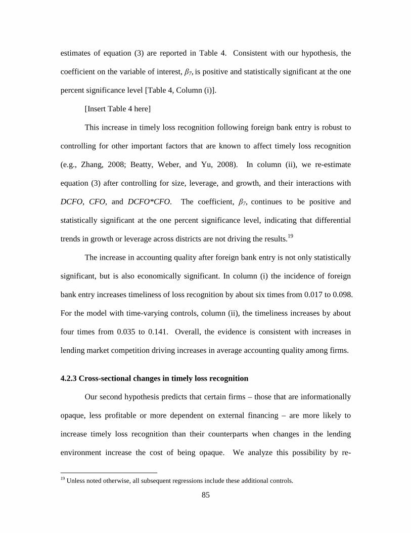
85
estimates of equation (3) are reported in Table 4. Consistent with our hypothesis, the
coefficient on the variable of interest, β7, is positive and statistically significant at the one
percent significance level [Table 4, Column (i)].
[Insert Table 4 here]
This increase in timely loss recognition following foreign bank entry is robust to
controlling for other important factors that are known to affect timely loss recognition
(e.g., Zhang, 2008; Beatty, Weber, and Yu, 2008). In column (ii), we re-estimate
equation (3) after controlling for size, leverage, and growth, and their interactions with
DCFO, CFO, and DCFO*CFO. The coefficient, β7, continues to be positive and
statistically significant at the one percent significance level, indicating that differential
trends in growth or leverage across districts are not driving the results.19
The increase in accounting quality after foreign bank entry is not only statistically
significant, but is also economically significant. In column (i) the incidence of foreign
bank entry increases timeliness of loss recognition by about six times from 0.017 to 0.098.
For the model with time-varying controls, column (ii), the timeliness increases by about
four times from 0.035 to 0.141. Overall, the evidence is consistent with increases in
lending market competition driving increases in average accounting quality among firms.
4.2.3 Cross-sectional changes in timely loss recognition
Our second hypothesis predicts that certain firms – those that are informationally
opaque, less profitable or more dependent on external financing – are more likely to
increase timely loss recognition than their counterparts when changes in the lending
environment increase the cost of being opaque. We analyze this possibility by re-
19 Unless noted otherwise, all subsequent regressions include these additional controls.

86
estimating equation (3) on subsamples of firms broken down by size, ownership,
profitability, and need for external financing. These estimates are reported in Tables 5-8.
Splitting the full sample into two groups based on the median of ROA, we find
that the increase in the timely loss recognition is greater, on average, among less
profitable firms. This is seen in Table 5, where the coefficient on the variable of interest,
β7, is positive and statistically significant at the one percent level for less profitable firms
but not for more profitable firms. This result suggests that less profitable firms
disproportionally increased accounting quality after foreign bank entry. This may reflect
an attempt by less profitable firms to mitigate the increased importance of agency costs
arising from information asymmetries between lenders and borrowers. We also find the
coefficient on DCFO*CFO is positive and significant for low profit firms but negative
and significant for high profit firms. A possible explanation could be that the agency cost
of debt for profitable firms is low, and banks do not demand high quality financial reports
for the ex-ante screening or ex-post monitoring of these firms.
[Insert Table 5 here]
Consistent with the argument that smaller firms are more informationally-opaque
and that foreign bank entry increases the cost of being opaque, we find the increase in
accounting quality is more pronounced among smaller firms. This is shown in Table 6
where the results are reported separately based on firms’ size. Timely loss recognition
increases among firms with assets below the median sample value [Table 6, Column (ii)],
but for firms with assets above the median value, we do not observe any average increase
in accounting quality [Table 6, Column (i)].
[Insert Table 6 here]
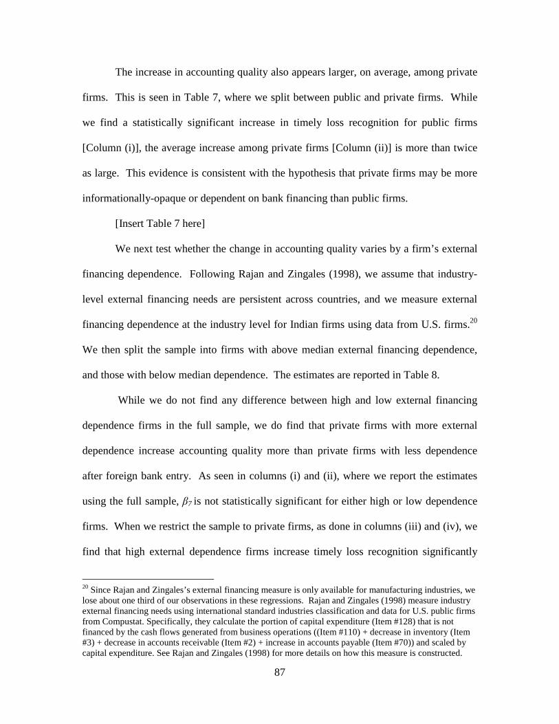
87
The increase in accounting quality also appears larger, on average, among private
firms. This is seen in Table 7, where we split between public and private firms. While
we find a statistically significant increase in timely loss recognition for public firms
[Column (i)], the average increase among private firms [Column (ii)] is more than twice
as large. This evidence is consistent with the hypothesis that private firms may be more
informationally-opaque or dependent on bank financing than public firms.
[Insert Table 7 here]
We next test whether the change in accounting quality varies by a firm’s external
financing dependence. Following Rajan and Zingales (1998), we assume that industry-
level external financing needs are persistent across countries, and we measure external
financing dependence at the industry level for Indian firms using data from U.S. firms.20
We then split the sample into firms with above median external financing dependence,
and those with below median dependence. The estimates are reported in Table 8.
While we do not find any difference between high and low external financing
dependence firms in the full sample, we do find that private firms with more external
dependence increase accounting quality more than private firms with less dependence
after foreign bank entry. As seen in columns (i) and (ii), where we report the estimates
using the full sample, β7 is not statistically significant for either high or low dependence
firms. When we restrict the sample to private firms, as done in columns (iii) and (iv), we
find that high external dependence firms increase timely loss recognition significantly
20 Since Rajan and Zingales’s external financing measure is only available for manufacturing industries, we lose about one third of our observations in these regressions. Rajan and Zingales (1998) measure industry external financing needs using international standard industries classification and data for U.S. public firms from Compustat. Specifically, they calculate the portion of capital expenditure (Item #128) that is not financed by the cash flows generated from business operations ((Item #110) + decrease in inventory (Item #3) + decrease in accounts receivable (Item #2) + increase in accounts payable (Item #70)) and scaled by capital expenditure. See Rajan and Zingales (1998) for more details on how this measure is constructed.
88
after foreign bank entry but low external financing dependence firms do not. The result
is consistent with the hypothesis that increased cost of being opaque is greater among
private firms with more dependence on external financing.
[Insert Table 8 here]
Taken together, the results in Tables 5-8 suggest that certain firms -- those that are
informationally opaque, less profitable, or more dependent on external funding -- are
more likely to increase their accounting quality when lending competition increases.
This evidence provides a new perspective to the potential effects of greater
financial market competition on lending relationships and the supply of credit to
informationally-opaque firms (Berger, Saunders, Scalise, and Udell, 1998; Degryse and
Ongena, 2007; Sapienza, 2002; and Zarutskie, 2006). The evidence suggests that firms’
opaqueness may not be completely fixed and that firms may actually be able to furnish
additional and easily verifiable information to lenders when lending market conditions
change. This possible adjustment by firms has been overlooked in the existing theoretical
literature that studies the potential effects of greater competition on the lending
relationships that firms may rely on (Boot and Thakor, 2000; Petersen and Rajan, 1995).
4.2.4. Timely loss recognition and access to credit
In this section, we test our third hypothesis of whether the increase in timely loss
recognition is correlated with firms’ access to credit markets. An underlying assumption
of the previous analyses is that lenders value timely loss recognition when making
lending decisions. Absent this, it would be difficult to understand why firms’ timely loss
recognition increases after foreign bank entry.
To test this underlying assumption, we analyze whether the increase in timely loss

89
recognition is accompanied by an increase in credit access among firms in districts that
experience foreign bank entry. To do this, we first re-estimate equation (3) using only
the firm-year observations of firms located in the eight districts that experience foreign
bank entry over the sample period. The estimates from using this more restrictive sample,
which are reported in column (i) of Table 9, confirm our earlier findings. The increase of
timely loss recognition after foreign entry is still positive and statistically significant at
the one percent level.
[Insert Table 9 here]
To test whether the increase in accounting quality is associated with better access
to credit for firms, we then divide the sample into firms that experience an increase in
debt levels after foreign entry and those that do not. This is done based on whether a
firms’ overall amount of bank borrowings increases or declines following foreign bank
entry. If a firm experiences a decline in bank borrowings after foreign bank entry, we
include it in the ‘debt-reduction’ group, otherwise we include it in the ‘no debt-reduction’
group. In total there are 1,672 firm-year observations that do not experience credit
declines, and 7,250 firm-year observations that do. If the increase in accounting quality
brings economic benefits to firms by alleviating credit constraints, then we expect that the
increase in timely loss recognition to be more pronounced for firms in the ‘no debt-
reduction’ group than firms in the ‘debt-reduction’ group.
In fact, this is exactly what the evidence appears to indicate. While firms in both
subsamples increased their timely loss recognition after foreign bank entry, the increase
is more pronounced among firms not experiencing a drop in overall credit. This is seen
in Table 9, columns (ii) and (iii), where the coefficient, β7, is almost twice the magnitude

90
(0.319 vs. 0.165) for the non-debt reduction subsample as for the debt reduction
subsample. The difference in β7 between the two groups of firms is statistically
significant at the one percent level (t=2.88). The result suggests more timely loss
recognition was associated with better access to credit markets following foreign bank
entry and that lenders value timely loss recognition when making lending decisions. The
improved accounting quality, however, may not be sufficient for opaque firms to
completely avoid the potential adverse outcomes of increased financial competition. As
seen in column (ii), many firms still exhibited a decline in overall bank borrowings
following foreign entry despite an average improvement in accounting quality.
4.3. Robustness tests
4.3.1 Selection bias
While there is no evidence in Table 3 that the levels of timely loss recognition
looked different across districts in India prior to foreign bank entry, one concern with the
above identification strategy is that foreign banks selectively entered districts where
levels of timely loss recognition were already trending upward or going to trend upward
in the future for reasons unrelated to foreign bank entry. For example, a selection bias
might occur if foreign banks choose to locate in regions of India in anticipation of future
improvements in accounting quality. If this occurred, the observed correlation between
accounting quality and foreign bank entry could be driven by foreign banks’ location
choice rather than an increase in financial competition.
The observed increases in accounting quality, however, do not appear to be driven
by foreign banks’ expectations of future accounting changes or some other selection bias.
First, accounting standards are set at the national level in India, which makes a foreign
91
bank’s choice of location based on expectations about regional changes in accounting
quality unlikely. It is also unclear why any changes in accounting regulation would
affect firms heterogeneously. Second, our earlier analysis in Table 9 suggests that
selection bias is not driving our results. In those estimates, the sample is restricted to
only firms located in the eight districts that experience foreign bank entry during the
sample time period. In doing this, we exclude the possibility that differential trends
between firms located in the districts with foreign bank entry and those that never
experience such entry are driving our earlier findings. As note earlier, foreign bank entry
is still positively associated with an increase in timely loss recognition in this restricted
sample [Table 9, column (i)]. Third, as shown in Dell’Arricia and Marquez (2004) and
Sengupta (2007), foreign banks are more likely to finance profitable domestic borrowers
due to their informational disadvantage. If foreign banks’ expectations of future
accounting changes drive our results, we would expect the increase in timely loss
recognition to be more pronounced for profitable firms than for less profitable firms.
However, this is in the opposite direction to what we find in Table 5.
4.3.2 Earnings time-series model
In this section, we conduct a sensitivity test by using equation (4) to test our first
hypothesis instead. Table 10 reports results of this exercise. Consistent with the results
reported in Table 4, the coefficient on the main variable of interest,7β , is negative and
statistically significant at the 5 percent level [column (i), Table 10] , suggesting that firms
increase timely loss recognition after foreign bank entry. The results are also robust to
including time-varying controls for firm size, leverage, and growth opportunities, and
their interactions with 1tD NI−
∆ , 1tNI−
∆ , and 1 1t tD NI NI− −
∆ ×∆ as shown in Column (ii).
92
[Insert Table 10 here]
5. Conclusion
Overall, we find evidence that firms attempt to reduce their opaqueness following
changes in the lending environment that may make such opaqueness more costly to the
firm. In particular, we find that the average level of accounting quality, as measured by
timely loss recognition, increases for firms located in the vicinity of new foreign banks
following their entry into India. The increases in accounting quality are also concentrated
among firms that may have a stronger incentive to alleviate financing constraints by
reducing information asymmetries and agency costs of debt. Specifically, we find that
smaller, less profitable, and private firms appear to respond to changes in the lending
environment the most. Private firms with greater dependence on external financing also
appear to respond more than the average firm, and lenders seem to value these changes.
Specifically, firms that improve the accounting quality the most were, on average, more
likely to experience an increase in their debt level after foreign bank entry.
This evidence provides a new perspective to the potential effects of greater credit
market competition on lending relationships and the supply of credit to informationally-
opaque firms. Our evidence suggests that firms’ inherent opaqueness may not be
completely fixed. Instead, firms potentially disadvantaged by the greater lending
competition seem to furnish additional, easily verifiable information to lenders to
mitigate the adverse impact on their credit access. To the authors’ knowledge, this
possible adjustment by firms has been overlooked in the existing literature and provides
an interesting avenue for future empirical work. The evidence also supports the argument
that greater financial competition can increase the cost of being opaque, particularly
among small, private, and less profitable firms.

93
Finally, our evidence suggests the financial market reforms may be another
channel through which countries may influence firms’ financial reporting. Contrary to
changes in regulations regarding disclosure and auditing rules, which directly affect firms’
accounting quality, our evidence suggests that an increase in lending market competition
may indirectly affect financial reporting by improving firms’ incentive to produce higher
quality statements.

References
Ahmed, A., B. Billings, R. Morton, and M. Harris, 2002, The Role of Accounting Conservatism in Mitigating Bondholder-Shareholder Conflicts over Dividend Policy and in Reducing Debt Costs, The Accounting Review 77(4): 867-890. Agarwal, S., Hauswald, R., 2007, Distance and information asymmetries in lending, Unpublished manuscript. Federal Reserve Bank of Chicago. Ball, R., S. P. Kothari, and R. Ashok, 2000, The effect of international institutional factors on properties of accounting earnings, Journal of Accounting and Economics 29(1): 1-51. Ball, R., 2001, Infrastructure Requirements for an Economically Efficient System of Public Financial Reporting and Disclosure, Brookings-Wharton Papers on Financial Services 2(1): 127-169. Ball, R. and L. Shivakumar, 2005, Earnings quality in UK private firms: comparative loss recognition timeliness, Journal of Accounting and Economics 39(1): 83-128. Ball, R., G. Sadka, and R. Ashok, 2008, Is Financial Reporting Shaped by Equity Markets or by Debt Markets? An International Study of Timeliness and Conservatism, Review of Accounting Studies 13 (2-3), 168-205. Basu, S., 1997, The conservatism principle and the asymmetric timeliness of earnings, Journal of Accounting and Economics 24(1): 3-37. Beatty, A., J. Weber, and J. Yu, 2008, Conservatism and Debt, Journal of Accounting and Economics 45(2-3): 154-174. Berger, A.N., Klapper, L.F., Peria, M.S.M., Zaidi, R., 2008. Bank ownership type and banking relationships, Journal of Financial Intermediation 1, 37-62. Berger, A. N., L. F. Klapper, and G.F. Udell, 2001, The ability of banks to lend to informationally opaque small businesses, Journal of Banking & Finance 25: 2127-2167. Berger, A. N., A. Saunders, J.M. Scalise, and G.F. Udell, 1998, The effects of bank mergers and acquisitions on small business lending, Journal of Financial Economics 50(2): 187-229. Bernanke, B. and M. Gertler, 1989, Agency Costs, Net Worth, and Business Fluctuations, American Economic Review 79(1): 14-31. Boot, A. W. A. and A. V. Thakor, 2000, Can Relationship Banking Survive Competition? The Journal of Finance 55(2): 679-713. Clarke, G. R. G., R. Cull, and M.S. Martinez Peria, 2006, Foreign bank participation and access to credit across firms in developing countries, Journal of Comparative Economics 34(4): 774-

95
795. Claessens, S., A. Demirguc-Kunt, and H. Huizinga, 2001, How does foreign bank entry affect the domestic banking market, Journal of Banking and Finance 25(5): 891-911. Dechow, P., 1994, Accounting earnings and cash flows as measures of firm performance: The role of accounting accruals, Journal of Accounting and Economics 18(1): 3-42. Dechow, P. M., S. P. Kothari, and R.L. Watts, 1998, The relation between earnings and cash flows, Journal of Accounting and Economics 25(2): 133-168. Degryse, H., Ongena, S., 2005, Distance, lending relationships, and competition, Journal of Finance 60, 231-266. Degryse, H. and S. Ongena, 2007, The impact of competition on bank orientation, Journal of Financial Intermediation 16(3): 399-424. Dell’Ariccia and G.R. Marquez, 2004, Information and bank credit allocation, Journal of Financial Economics 72: 185-214. Detragiache, E., Gupta, P. and Tressel, T., 2008, Foreign Banks in Poor Countries: Theory and Evidence, Journal of Finance, 63(5). Diamond, D., 1984, Financial Intermediation and Delegated Monitoring, Review of Economic Studies 51(3): 393-414. Giannetti, M. and S. Ongena, 2009a, "Financial Integration and Firm Performance: Evidence from Foreign Bank Entry in Emerging Markets, Review of Finance 13(2): 181-223. Giannetti, M. and S. Ongena, 2009b, "Lending by Example": Direct and Indirect Effects of Foreign Banks in Emerging Markets, Working paper, Stockholm School of Economics and Tilburg University. Gormley, Todd A., 2007, Costly Information, Foreign Entry, and Credit Access, working paper. Gormley, Todd A., 2008, The Impact of Foreign Bank Entry in Emerging Markets: Evidence from India, forthcoming, Journal of Financial Intermediation. Guay, W. R., 2008, Conservative financial reporting, debt covenants, and the agency costs of debt, Journal of Accounting and Economics 45(2-3): 175-180. Haber, S. H., and A. Musacchio, 2004, Foreign Banks and the Mexican Economy, 1997-2004, Division of Research, Harvard Business School. Kothari, S. P., 2001, Capital markets research in accounting, Journal of Accounting and Economics 31(1-3): 105-231.

96
LaFond, R. and R. L. Watts, 2007, The information role of conservative financial statements, The Accounting Review. Lensink, R. and N. Hermes, 2004, The short-term effects of foreign bank entry on domestic bank behaviour: does economic development matter? Journal of Banking and Finance 28, 553-568. Leuz, C., Nanda, D., and P., Wysocki, 2003, Earnings management and investor protection: an international comparison, Journal of Financial Economics 69, 505-527. Mian, A., 2006, Distance Constraints: The Limits of Foreign Lending in Poor Economies, The Journal of Finance 61(3): 1465-1505. Moerman, R., 2008, The role of information asymmetry and financial reporting quality in debt contracting: Evidence from the secondary loan market, Journal of Accounting and Economics. Petersen, M. A. and R. G. Rajan, 1995, The Effect of Credit Market Competition on Lending Relationships, Quarterly Journal of Economics 110(2): 407-443. Petersen, M.A., Rajan, R.G., 2002, Does distance still matter? The information revolution in small business lending, Journal of Finance 57, 2533-2570. Rajan, R.G. and L. Zingales, 1998, Financial Dependence and Growth, American Economic Review 88(3): 559-586. Ramakrishnan, R. and A. V. Thakor, 1984, Information Reliability and a Theory of Financial Intermediation, Review of Economic Studies 51(3): 415-32. Rice, T. and P. E. Strahan, 2009, Does Credit Competition Affect Small-Firm Finance? Journal of Finance, forthcoming. Roberts, M. and A. Sufi, 2009, Control Rights and Capital Structure: An Empirical Investigation, Journal of Finance, 64(4), 1657-1695. Roychowdhury, S. and R. L. Watts, 2007, Asymmetric timeliness of earnings, market-to-book and conservatism in financial reporting, Journal of Accounting and Economics 44(1-2): 2-31. Sapienza, P., 2002, The Effects of Banking Mergers on Loan Contracts, The Journal of Finance 57(1): 329-367. Sengupta, R., 2007, Foreign entry and bank competition, Journal of Financial Economics 84(2): 502-528. Stein, J. C., 2002, Information Production and Capital Allocation: Decentralized versus Hierarchical Firms, Journal of Finance, 57(5): 1891-1921. Watts, R. L., 2003a, Conservatism in Accounting Part I: Explanations and Implications,

97
Accounting Horizons 17(3): 207-222. Watts, R. L., 2003b, Conservatism in Accounting Part II: Evidence and Research Opportunities, Accounting Horizons 17(4): 287-302. Watts, R. and J. Zimmerman, 1986, Positive Accounting Research, Englewood Cliffs, NJ: Prentice Hall. Watts, R. L. and J. L. Zimmerman, 1990, Positive Accounting Theory: A Ten Year Perspective, The Accounting Review 65(1): 131-156. Zarutskie, R., 2006, Evidence on the effects of bank competition on firm borrowing and investment, Journal of Financial Economics 81(3): 503-537. Zhang, J., 2008, The contracting benefits of accounting conservatism to lenders and borrowers, Journal of Accounting and Economics 45(1): 27-54.
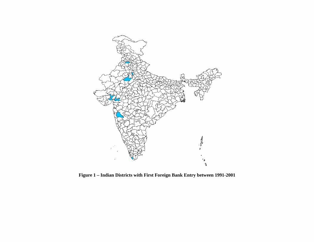
Figure 1 – Indian Districts with First Foreign Bank Entry between 1991-2001
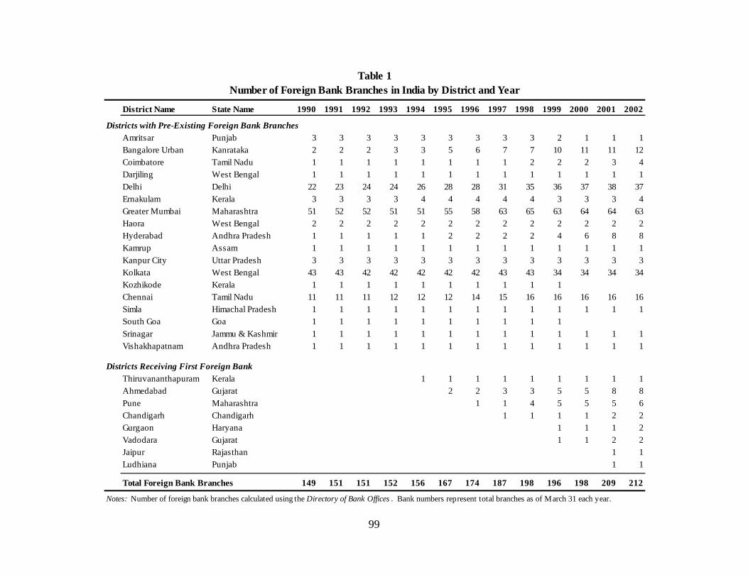
99
District Name State Name 1990 1991 1992 1993 1994 1995 19961997 1998 1999 2000 2001 2002
Districts with Pre-Existing Foreign Bank BranchesAmritsar Punjab 3 3 3 3 3 3 3 3 3 2 1 1 1Bangalore Urban Kanrataka 2 2 2 3 3 5 6 7 7 10 11 11 12Coimbatore Tamil Nadu 1 1 1 1 1 1 1 1 2 2 2 3 4Darjiling West Bengal 1 1 1 1 1 1 1 1 1 1 1 1 1
Delhi Delhi 22 23 24 24 26 28 28 31 35 36 37 38 37Ernakulam Kerala 3 3 3 3 4 4 4 4 4 3 3 3 4Greater Mumbai Maharashtra 51 52 52 51 51 55 58 63 65 63 64 64 63Haora West Bengal 2 2 2 2 2 2 2 2 2 2 2 2 2Hyderabad Andhra Pradesh 1 1 1 1 1 2 2 2 2 4 6 8 8Kamrup Assam 1 1 1 1 1 1 1 1 1 1 1 1 1
Kanpur City Uttar Pradesh 3 3 3 3 3 3 3 3 3 3 3 3 3Kolkata West Bengal 43 43 42 42 42 42 42 43 43 34 34 34 34Kozhikode Kerala 1 1 1 1 1 1 1 1 1 1Chennai Tamil Nadu 11 11 11 12 12 12 14 15 16 16 16 16 16Simla Himachal Pradesh 1 1 1 1 1 1 1 1 1 1 1 1 1South Goa Goa 1 1 1 1 1 1 1 1 1 1
Srinagar Jammu & Kashmir 1 1 1 1 1 1 1 1 1 1 1 1 1Vishakhapatnam Andhra Pradesh 1 1 1 1 1 1 1 1 1 1 1 1 1
Districts Receiving First Foreign BankThiruvananthapuram Kerala 1 1 1 1 1 1 1 1 1Ahmedabad Gujarat 2 2 3 3 5 5 8 8
Pune Maharashtra 1 1 4 5 5 5 6Chandigarh Chandigarh 1 1 1 1 2 2Gurgaon Haryana 1 1 1 2Vadodara Gujarat 1 1 2 2Jaipur Rajasthan 1 1Ludhiana Punjab 1 1
Total Foreign Bank Branches 149 151 151 152 156 167 174 187198 196 198 209 212
Notes: Number of foreign bank branches calculated using the Directory of Bank Offices. Bank numbers represent total branches as of March 31 each year.
Number of Foreign Bank Branches in India by District and YearTable 1
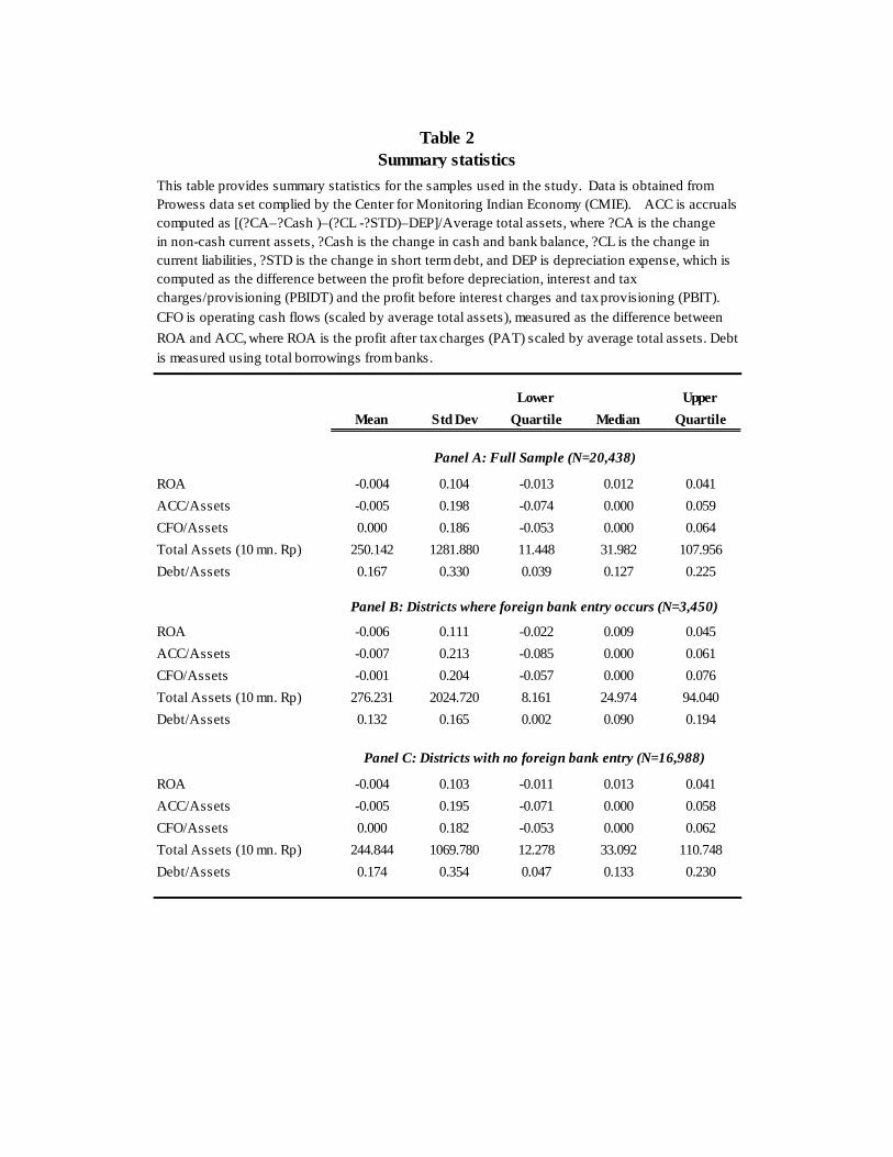
Lower Upper
Mean Std Dev Quartile Median Quartile
ROA -0.004 0.104 -0.013 0.012 0.041
ACC/Assets -0.005 0.198 -0.074 0.000 0.059
CFO/Assets 0.000 0.186 -0.053 0.000 0.064
Total Assets (10 mn. Rp) 250.142 1281.880 11.448 31.982 107.956
Debt/Assets 0.167 0.330 0.039 0.127 0.225
ROA -0.006 0.111 -0.022 0.009 0.045
ACC/Assets -0.007 0.213 -0.085 0.000 0.061
CFO/Assets -0.001 0.204 -0.057 0.000 0.076
Total Assets (10 mn. Rp) 276.231 2024.720 8.161 24.974 94.040
Debt/Assets 0.132 0.165 0.002 0.090 0.194
ROA -0.004 0.103 -0.011 0.013 0.041
ACC/Assets -0.005 0.195 -0.071 0.000 0.058
CFO/Assets 0.000 0.182 -0.053 0.000 0.062
Total Assets (10 mn. Rp) 244.844 1069.780 12.278 33.092 110.748
Debt/Assets 0.174 0.354 0.047 0.133 0.230
Panel B: Districts where foreign bank entry occurs (N=3,450)
Panel C: Districts with no foreign bank entry (N=16,988)
This table provides summary statistics for the samples used in the study. Data is obtained from Prowess data set complied by the Center for Monitoring Indian Economy (CMIE). ACC is accruals computed as [(?CA–?Cash )–(?CL -?STD)–DEP]/Average total assets, where ?CA is the change in non-cash current assets, ?Cash is the change in cash and bank balance, ?CL is the change in current liabilities, ?STD is the change in short term debt, and DEP is depreciation expense, which is computed as the difference between the profit before depreciation, interest and tax charges/provisioning (PBIDT) and the profit before interest charges and tax provisioning (PBIT). CFO is operating cash flows (scaled by average total assets), measured as the difference between
ROA and ACC, where ROA is the profit after tax charges (PAT) scaled by average total assets. Debt is measured using total borrowings from banks.
Table 2Summary statistics
Panel A: Full Sample (N=20,438)
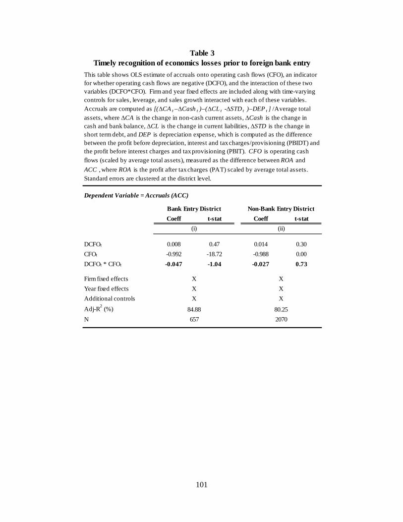
101
Coeff t-stat Coeff t-stat
DCFOt 0.008 0.47 0.014 0.30
CFOt -0.992 -18.72 -0.988 0.00
DCFOt * CFOt -0.047 -1.04 -0.027 0.73
Firm fixed effects
Year fixed effects
Additional controls
Adj-R2 (%)
N
X X
Bank Entry District Non-Bank Entry District
X X
657 2070
84.88 80.25
X X
(i) (ii)
Timely recognition of economics losses prior to foreign bank entryThis table shows OLS estimate of accruals onto operating cash flows (CFO), an indicator for whether operating cash flows are negative (DCFO), and the interaction of these two variables (DCFO*CFO). Firm and year fixed effects are included along with time-varying controls for sales, leverage, and sales growth interacted with each of these variables. Accruals are computed as [(∆CAt –∆Casht )–(∆CL t -∆STDt )–DEPt ] /Average total assets, where ∆CA is the change in non-cash current assets, ∆Cash is the change in cash and bank balance, ∆CL is the change in current liabilities, ∆STD is the change in short term debt, and DEP is depreciation expense, which is computed as the difference between the profit before depreciation, interest and tax charges/provisioning (PBIDT) and the profit before interest charges and tax provisioning (PBIT). CFO is operating cash flows (scaled by average total assets), measured as the difference between ROA and
ACC , where ROA is the profit after tax charges (PAT) scaled by average total assets. Standard errors are clustered at the district level.
Table 3
Dependent Variable = Accruals (ACC)
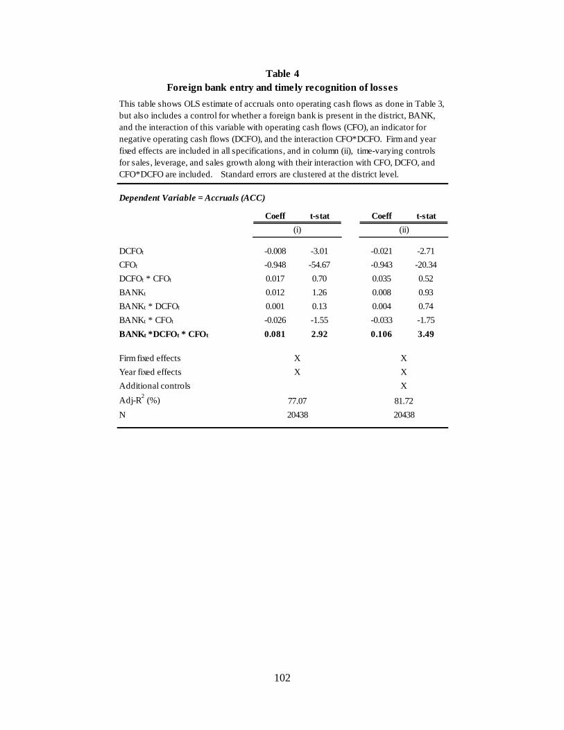
102
Dependent Variable = Accruals (ACC)
Coeff t-stat Coeff t-stat
DCFOt -0.008 -3.01 -0.021 -2.71
CFOt -0.948 -54.67 -0.943 -20.34
DCFOt * CFOt 0.017 0.70 0.035 0.52
BANK t 0.012 1.26 0.008 0.93
BANK t * DCFOt 0.001 0.13 0.004 0.74
BANK t * CFOt -0.026 -1.55 -0.033 -1.75
BANK t *DCFO t * CFOt 0.081 2.92 0.106 3.49
Firm fixed effects
Year fixed effects
Additional controls
Adj-R2 (%)
N
X
This table shows OLS estimate of accruals onto operating cash flows as done in Table 3, but also includes a control for whether a foreign bank is present in the district, BANK, and the interaction of this variable with operating cash flows (CFO), an indicator for negative operating cash flows (DCFO), and the interaction CFO*DCFO. Firm and year fixed effects are included in all specifications, and in column (ii), time-varying controls for sales, leverage, and sales growth along with their interaction with CFO, DCFO, and CFO*DCFO are included. Standard errors are clustered at the district level.
Table 4Foreign bank entry and timely recognition of losses
(i) (ii)
X X
X X
77.07 81.72
20438 20438
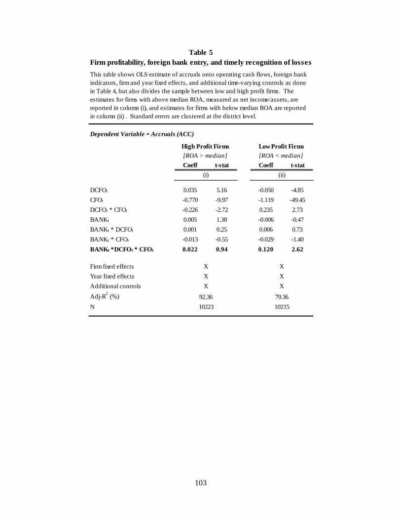
103
Dependent Variable = Accruals (ACC)
Coeff t-stat Coeff t-stat
DCFOt 0.035 5.16 -0.050 -4.85
CFOt -0.770 -9.97 -1.119 -49.45
DCFOt * CFOt -0.226 -2.72 0.235 2.73
BANK t 0.005 1.38 -0.006 -0.47
BANK t * DCFOt 0.001 0.25 0.006 0.73
BANK t * CFOt -0.013 -0.55 -0.029 -1.40
BANK t *DCFO t * CFOt 0.022 0.94 0.120 2.62
Firm fixed effects
Year fixed effects
Additional controls
Adj-R2 (%)
N 10223 10215
Low Profit Firms[ROA > median] [ROA < median]
X X
92.36 79.36
(ii)
X
X
X
X
(i)
High Profit Firms
Table 5Firm profitability, foreign bank entry, and timely recognition of losses
This table shows OLS estimate of accruals onto operating cash flows, foreign bank indicators, firm and year fixed effects, and additional time-varying controls as done in Table 4, but also divides the sample between low and high profit firms. The estimates for firms with above median ROA, measured as net income/assets, are reported in column (i), and estimates for firms with below median ROA are reported in column (ii) . Standard errors are clustered at the district level.
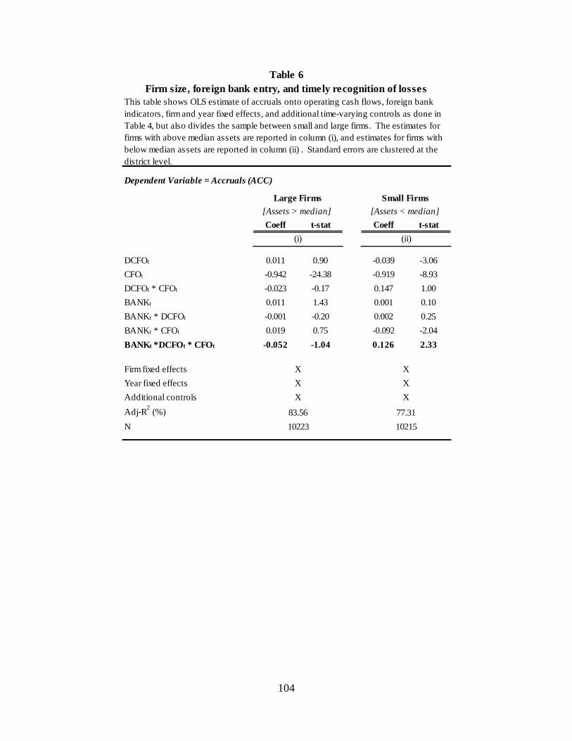
104
Dependent Variable = Accruals (ACC)
Coeff t-stat Coeff t-stat
DCFOt 0.011 0.90 -0.039 -3.06
CFOt -0.942 -24.38 -0.919 -8.93
DCFOt * CFOt -0.023 -0.17 0.147 1.00
BANK t 0.011 1.43 0.001 0.10
BANK t * DCFOt -0.001 -0.20 0.002 0.25
BANK t * CFOt 0.019 0.75 -0.092 -2.04
BANK t *DCFO t * CFOt -0.052 -1.04 0.126 2.33
Firm fixed effects
Year fixed effects
Additional controls
Adj-R2 (%)
N
83.56 77.31
10223 10215
X X
X X
(i) (ii)
X X
[Assets > median] [Assets < median]
Table 6Firm size, foreign bank entry, and timely recognition of losses
This table shows OLS estimate of accruals onto operating cash flows, foreign bank indicators, firm and year fixed effects, and additional time-varying controls as done in Table 4, but also divides the sample between small and large firms. The estimates for firms with above median assets are reported in column (i), and estimates for firms with below median assets are reported in column (ii) . Standard errors are clustered at the district level.
Large Firms Small Firms
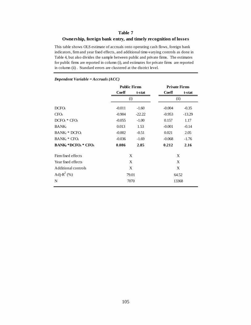
105
Dependent Variable = Accruals (ACC)
Coeff t-stat Coeff t-stat
DCFOt -0.011 -1.60 -0.004 -0.35
CFOt -0.904 -22.22 -0.953 -13.29
DCFOt * CFOt -0.055 -1.00 0.157 1.17
BANK t 0.013 1.53 -0.001 -0.14
BANK t * DCFOt -0.002 -0.51 0.021 2.05
BANK t * CFOt -0.036 -1.69 -0.068 -1.76
BANK t *DCFO t * CFOt 0.086 2.85 0.212 2.16
Firm fixed effects
Year fixed effects
Additional controls
Adj-R2 (%)
N
79.01 64.52
7070 13368
X X
X X
(i) (ii)
X X
Table 7Ownership, foreign bank entry, and timely recognition of losses
This table shows OLS estimate of accruals onto operating cash flows, foreign bank indicators, firm and year fixed effects, and additional time-varying controls as done in Table 4, but also divides the sample between public and private firms. The estimates for public firms are reported in column (i), and estimates for private firms are reported in column (ii) . Standard errors are clustered at the district level.
Public Firms Private Firms
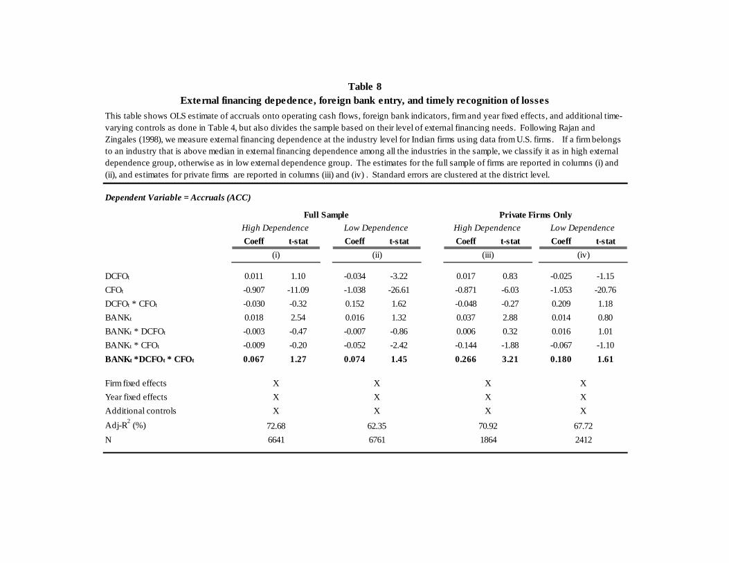
Dependent Variable = Accruals (ACC)
Coeff t-stat Coeff t-stat Coeff t-stat Coeff t-stat
DCFOt 0.011 1.10 -0.034 -3.22 0.017 0.83 -0.025 -1.15
CFOt -0.907 -11.09 -1.038 -26.61 -0.871 -6.03 -1.053 -20.76
DCFOt * CFOt -0.030 -0.32 0.152 1.62 -0.048 -0.27 0.209 1.18
BANK t 0.018 2.54 0.016 1.32 0.037 2.88 0.014 0.80
BANK t * DCFOt -0.003 -0.47 -0.007 -0.86 0.006 0.32 0.016 1.01
BANK t * CFOt -0.009 -0.20 -0.052 -2.42 -0.144 -1.88 -0.067 -1.10
BANK t *DCFO t * CFOt 0.067 1.27 0.074 1.45 0.266 3.21 0.180 1.61
Firm fixed effects
Year fixed effects
Additional controls
Adj-R2 (%)
N 1864 2412
This table shows OLS estimate of accruals onto operating cash flows, foreign bank indicators, firm and year fixed effects, and additional time-varying controls as done in Table 4, but also divides the sample based on their level of external financing needs. Following Rajan and Zingales (1998), we measure external financing dependence at the industry level for Indian firms using data from U.S. firms. If a firm belongs to an industry that is above median in external financing dependence among all the industries in the sample, we classify it as in high external dependence group, otherwise as in low external dependence group. The estimates for the full sample of firms are reported in columns (i) and (ii), and estimates for private firms are reported in columns (iii) and (iv) . Standard errors are clustered at the district level.
70.92 67.72
(iii) (iv)
72.68 62.35
6641
Table 8External financing depedence, foreign bank entry, and timely recognition of losses
Full Sample Private Firms Only
X X
X X
X X
High Dependence Low Dependence
6761
X X
X X
High Dependence Low Dependence
(i) (ii)
X X
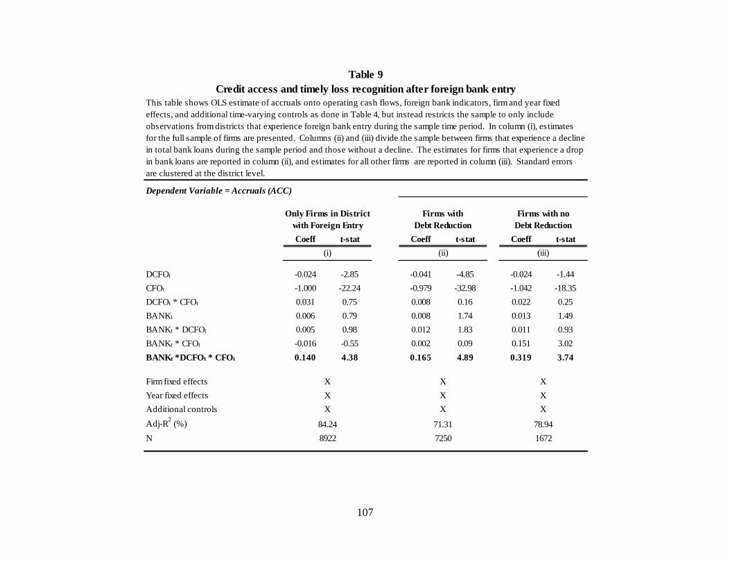
107
Dependent Variable = Accruals (ACC)
Coeff t-stat Coeff t-stat Coeff t-stat
DCFOt -0.024 -2.85 -0.041 -4.85 -0.024 -1.44
CFOt -1.000 -22.24 -0.979 -32.98 -1.042 -18.35
DCFOt * CFOt 0.031 0.75 0.008 0.16 0.022 0.25
BANK t 0.006 0.79 0.008 1.74 0.013 1.49
BANK t * DCFOt 0.005 0.98 0.012 1.83 0.011 0.93
BANK t * CFOt -0.016 -0.55 0.002 0.09 0.151 3.02
BANK t *DCFO t * CFOt 0.140 4.38 0.165 4.89 0.319 3.74
Firm fixed effects
Year fixed effects
Additional controls
Adj-R2 (%)
N
X X
8922
X
84.24
7250
Table 9Credit access and timely loss recognition after foreign bank entry
This table shows OLS estimate of accruals onto operating cash flows, foreign bank indicators, firm and year fixed effects, and additional time-varying controls as done in Table 4, but instead restricts the sample to only include observations from districts that experience foreign bank entry during the sample time period. In column (i), estimates for the full sample of firms are presented. Columns (ii) and (iii) divide the sample between firms that experience a decline in total bank loans during the sample period and those without a decline. The estimates for firms that experience a drop in bank loans are reported in column (ii), and estimates for all other firms are reported in column (iii). Standard errors are clustered at the district level.
Firms with Debt Reduction
Firms with no Debt Reduction
Only Firms in District with Foreign Entry
X
71.31 78.94
(iii)
X
X
(i) (ii)
1672
X X
X
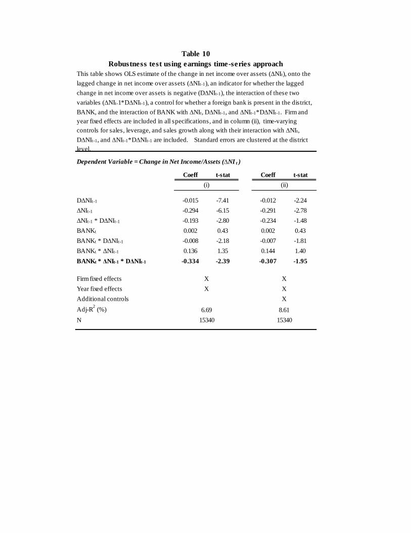
Dependent Variable = Change in Net Income/Assets (∆NI t )
Coeff t-stat Coeff t-stat
D∆NIt-1 -0.015 -7.41 -0.012 -2.24
∆NIt-1 -0.294 -6.15 -0.291 -2.78
∆NIt-1 * D∆NIt-1 -0.193 -2.80 -0.234 -1.48
BANK t 0.002 0.43 0.002 0.43
BANK t * D∆NIt-1 -0.008 -2.18 -0.007 -1.81
BANK t * ∆NIt-1 0.136 1.35 0.144 1.40
BANK t * ∆NIt-1 * D∆NIt-1 -0.334 -2.39 -0.307 -1.95
Firm fixed effects
Year fixed effects
Additional controls
Adj-R2 (%)
N
6.69 8.61
15340 15340
X X
X
X X
Table 10Robustness test using earnings time-series approach
This table shows OLS estimate of the change in net income over assets (∆NIt), onto the
lagged change in net income over assets (∆NIt-1), an indicator for whether the lagged
change in net income over assets is negative (D∆NIt-1), the interaction of these two
variables (∆NIt-1*D∆NIt-1), a control for whether a foreign bank is present in the district,
BANK, and the interaction of BANK with ∆NIt, D∆NIt-1, and ∆NIt-1*D∆NIt-1. Firm and year fixed effects are included in all specifications, and in column (ii), time-varying controls for sales, leverage, and sales growth along with their interaction with ∆NIt,
D∆NIt-1, and ∆NIt-1*D∆NIt-1 are included. Standard errors are clustered at the district level.
(i) (ii)
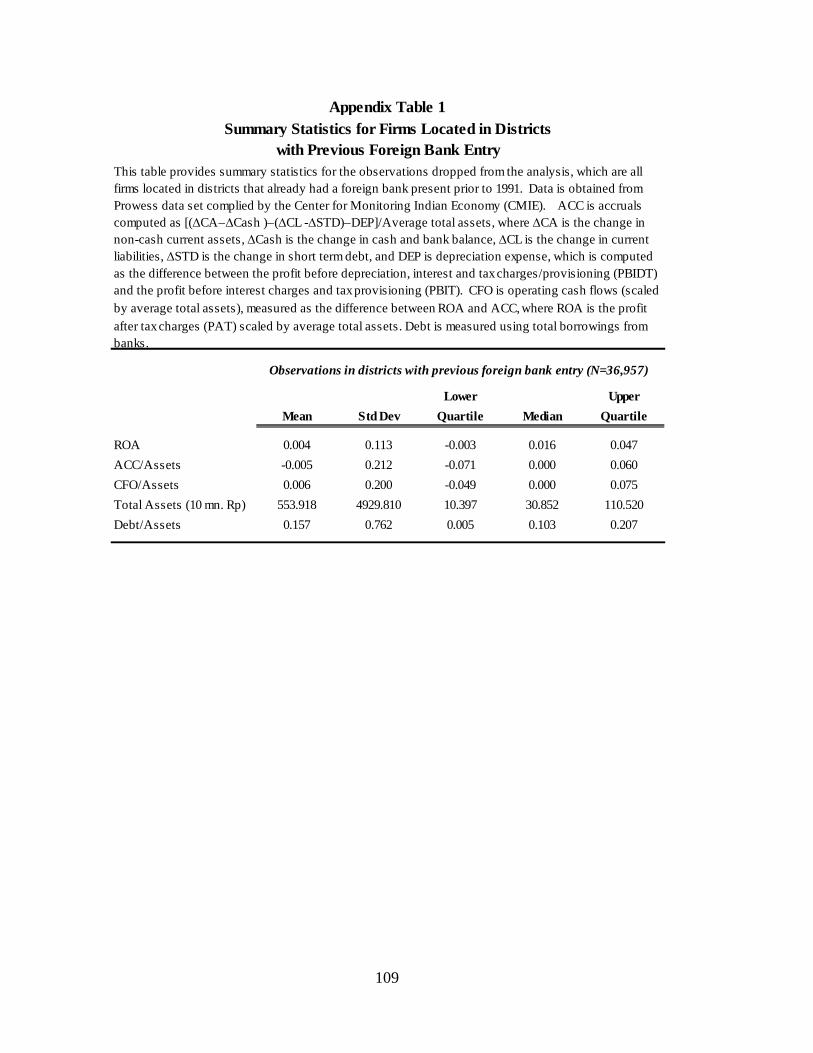
109
Lower Upper
Mean Std Dev Quartile Median Quartile
ROA 0.004 0.113 -0.003 0.016 0.047
ACC/Assets -0.005 0.212 -0.071 0.000 0.060
CFO/Assets 0.006 0.200 -0.049 0.000 0.075
Total Assets (10 mn. Rp) 553.918 4929.810 10.397 30.852 110.520
Debt/Assets 0.157 0.762 0.005 0.103 0.207
Appendix Table 1Summary Statistics for Firms Located in Districts
with Previous Foreign Bank EntryThis table provides summary statistics for the observations dropped from the analysis, which are all firms located in districts that already had a foreign bank present prior to 1991. Data is obtained from Prowess data set complied by the Center for Monitoring Indian Economy (CMIE). ACC is accruals computed as [(∆CA–∆Cash )–(∆CL -∆STD)–DEP]/Average total assets, where ∆CA is the change in non-cash current assets, ∆Cash is the change in cash and bank balance, ∆CL is the change in current liabilities, ∆STD is the change in short term debt, and DEP is depreciation expense, which is computed as the difference between the profit before depreciation, interest and tax charges/provisioning (PBIDT) and the profit before interest charges and tax provisioning (PBIT). CFO is operating cash flows (scaled by average total assets), measured as the difference between ROA and ACC, where ROA is the profit after tax charges (PAT) scaled by average total assets. Debt is measured using total borrowings from banks.
Observations in districts with previous foreign bank entry (N=36,957)
110
Chapter IV
Conditional Accounting Conservatism and Future Negative Surprises: An Empirical Investigation
Bong Hwan Kim
Olin School of Business Washington University in St. Louis
Mikhail Pevzner School of Management
George Mason University
Abstract: We investigate whether conditional accounting conservatism has informational benefits to shareholders. We find some evidence that higher current conditional conservatism is associated with lower probability of future bad news, proxied by missing analyst forecasts, earnings decreases, and dividend decreases. Second, we find weak evidence that the stock market reacts stronger (weaker) to good (bad) earnings news of more conditionally conservative firms. Thus, we provide additional evidence that conditional conservatism affects stock prices.
This paper is forthcoming at Journal of Accounting and Public Policy.
1. Introduction
We examine whether conditional accounting conservatism (hereafter conditional
conservatism) has benefits to stockholders, an issue with important public policy
implications. Conditional conservatism is reflected in the firms’ policies of timely
recognition of bad news and delayed recognition of good news, i.e., conditional
conservatism places higher verifiability standard on good earnings news recognition, as
opposed to bad earnings news recognition.
Conditional conservatism has influenced accounting rules for a very long time and is
arguably one of the most fundamental principles in accounting (Watts, 2003). However,
recently both the U.S. GAAP and International Financial Reporting Standards (IFRS) have
been making a strong push for “fair value” accounting. The fair value principle essentially
demands symmetric timeliness: both good news and bad news are recognized, and
recognition of good news is not deferred. In other words, the fair value principle is an
opposite of the conditional conservatism in accounting, which requires deferred recognition
of good news.
Fair value principle introduces earlier recognition of unrealized gains, and, if fair
values subsequently decrease, recognition of unrealized losses. One reason for adopting the
fair value principle is an assumption that it improves transparency of the accounting
information. However, it could be argued that earlier recognition of unrealized gains distorts
the true economic picture of a firm because application of fair value could lead to
contracting inefficiencies, stronger earnings volatility, and, when fair values decrease,
firms’ having to record future losses of greater magnitude. In contrast, the application of
conditional conservatism potentially results in lower volatility of earnings, contracting
112
benefits, which protect lenders (Watts, 2003), reductions in firms’ litigation risk (Khan and
Watts, 2007), and limiting of wealth transfers to larger shareholders (LaFond and
Roychowdhury, 2008).
The examination of merits of accounting conservatism is especially important
because fair value application also has some potential drawbacks. First, because the
application of fair value also requires discretion, especially in the situations when no quoted
market prices are available, it could be opportunistic (Ramanna and Watts, 2007). In
addition, some critics blame the severity of the recent sub-prime mortgage crisis on fair
value (Katz, 2008) because fair value application resulted in massive write-downs of
mortgage-backed securities to “fire sale” prices. The application of conditional
conservatism could have prevented such massive write-downs because it would not have
allowed earlier recognition of unrealized gains. In light of these claims, it is important to
examine whether conditional conservatism has benefits for stockholders.
Thus, we examine whether 1) higher levels of conditional conservatism are
associated with lower levels of future bad news, and 2) whether cross-sectional variation in
levels of conditional conservatism affects the stock market’s reactions to firms’ good news
and bad news earnings announcements. Our goal is to provide evidence of whether greater
levels of conditional conservatism worsen or improve firms’ information asymmetry by
forcing the earlier recognition of the bad earnings news in accounting earnings. Such early
bad news recognition implies that conditional conservatism is associated with less future
bad news. In addition, if conditional conservatism is associated with lower levels of future
bad news and the market perceives such association to be economically significant, we

113
could also expect that the market rewards more conservative firms with more positive (less
negative) reaction to good (bad) news earnings announcements.
To address whether conservatism leads to lower likelihood of future bad news, we
examine the association of several proxies of conservatism with a) likelihood of firms’
missing analyst forecasts, 2) likelihood of future earnings decreases, and 3) likelihood of
future dividend decreases. We find evidence that several proxies of conservatism are
associated with lower likelihoods of future bad news.
To address whether the stock market values conservatism, we run short-window
stock market response to earnings news (ERC) regressions, with added interactions of
conservatism and earnings surprises. We find weak evidence that the market rewards more
conservative firms with more positive (less negative) reaction to good (bad) news earnings
announcements.
Our study proceeds as follows. Section 2 develops our hypotheses. Section 3
describes our sample and research design. Section 4 describes our results, and Section 5
concludes.
2. Motivation 2.1 Literature Review
The empirical accounting literature provides evidence that debt-holders demand
higher levels of conditional conservatism in order to reduce potentially negative impact of
agency conflicts arising between borrowers and lenders.38 However, whether greater levels
38 Zhang (2008) shows that more conservative firms experience faster debt covenant violations, thus faster “triggering lenders’ alarm”. Kim (2007) shows that borrowers’ conservatism level does not decrease after borrowing. Ahmed et al. (2002) show that debt-holders view conservatism as means of minimizing wealth transfers from debt-holders to shareholders and thus reward more conservative
114
of conditional conservatism have impact on equity market is an open empirical question.
Two opposing explanations of the role of conservatism (conditional or unconditional) in the
equity markets exist: 1) conservatism is beneficial to shareholders, and 2) conservatism is
potentially harmful to shareholders because it decreases firms’ information quality.
Positive role of conservatism: conservatism increases the amount of information
in the market. Theory suggests several informational benefits of conservatism, such as
reducing benefits of earnings management (Chen et al., 2007), improving information
quality (Fan and Zhang, 2007), and signaling of managerial private information (Bagnoli
and Watts, 2005). The unifying underlying theme of these studies is that conservatism
improves information quality and thus should reduce information asymmetry between
informed and uninformed investors. Several empirical studies test this theoretical prediction.
LaFond and Watts (2008) and Khan and Watts (2007) examine the associations between
conditional conservatism and firm liquidity levels. These studies provide evidence showing
that decreases in firm liquidity are followed by increases in firm conservatism. However,
these papers cannot unambiguously conclude that conditional conservatism is beneficial to
stockholders because liquidity proxies used in these studies, namely Probability of Informed
Trade (PIN) and bid-ask spread, have been criticized as having no stock price impact.39
Absent such significant price impact, the value of conservatism to stockholders is
questionable.
borrowers with lower cost of debt. Moerman (2009) shows that more conditionally conservative firms are rewarded with lower bid-ask spreads on the secondary loan markets. Ball et al. (2008) show that conservatism leads under-writers to hold lower stake in issued loans. Altogether, these studies provide strong evidence that conservatism is an effective tool in reducing information asymmetry between borrowers and lenders. 39 In particular, Mohanram and Rajgopal (2009) show that the negative association of PIN and realized return only exists in small firms. More importantly, Duarte and Yong (2009) show that the negative association of PIN and expected returns is not driven by information risk, but by stocks’ illiquidity. Easley et al (2003) show that PIN subsumes bid-ask spread as the determinant of expected returns.

115
Balachandran and Mohanram (2008) find no negative impact of unconditional
conservatism on value-relevance of earnings. For firms with decreasing unconditional
conservatism levels, they find that value relevance of book values declines, suggesting that
the market views book values of such firms as weak predictors of firms’ values.
Balachandran and Mohanram’s results are still important from the policy-setting perspective
because they show that greater conservatism results in a stronger market response to the
accounting numbers. Specifically, to the extent that conservatism reduces perceived
variance of future expected cash flows (because conservatism makes estimates of such cash
flows more reliable), the market should reward more conservative firms with higher
valuation multiples. Thus, following the logic of Barth et al. (2001) and extant value
relevance literature, standard setters should adopt more conservative accounting policies,
which will result in better valuations. However, Balachandran and Mohanram’s paper relies
on long window association study research design approach, making it more difficult to
identify the exact channel by which unconditional conservatism makes information more
transparent. In addition, Holthausen and Watts (2001) question standard setting implications
of more value relevant accounting numbers, suggesting that the objectives of standard
setters need not be based on whether something is more or less value relevant, but rather on
the contracting, regulatory, and other implications of the accounting policies. Hence, more
research in this area is needed.
Following Balachandran and Mohanram (2008), Li (2007) shows that unconditional
conservatism reduces uncertainty in analyst forecasts. Li shows that unconditional
conservatism, measured by the Beaver and Ryan (2000) model, is negatively associated
with analyst forecast errors for good news and mild bad news cases, but is positively
116
associated with extreme bad news forecast errors. These results suggest that unconditional
conservatism results in greater analyst forecast accuracy with respect to mild bad news and
may reduce analyst forecast optimism with respect to good news. Li also finds that the level
of overall analyst uncertainty is negatively associated with ex-ante levels of unconditional
conservatism. However, because this study is focused only on un-conditional conservatism,
it is unclear whether similar results hold for conditional conservatism measures.
Negative view of conservatism: conservatism reduces information quality and
hurts investors. Several papers document the association of higher conservatism levels with
lower earnings persistence. Paek et al. (2007) show that firms with more conditionally
conservative reported earnings have lower earnings multiples because conditional
conservatism reduces earnings persistence. Their result suggests that conditional
conservatism introduces noise in the earnings process, making earnings less value-relevant.
Such a result is also consistent with Financial Accounting Standards Boards (FASB)’s
statements, suggesting that conservatism increases information asymmetry (LaFond and
Watts, 2008). However, the implications of this result for usefulness of conservatism are not
necessarily clear. More persistent earnings numbers are associated with lower uncertainty
about firms’ future performance, and make it easier for investors to correctly estimate
earnings multiples and forecast stock prices. At the same time, given well documented
results that bad news in general is less persistent, lower earnings multiples are expected for
bad news firms in general, and for conservative firms in particular.40 The latter implication
suggests that conservatism does not necessarily hurt users of financial information.
In addition, conservatism (whether conditional or unconditional) could also be used
to shield excessive profits from regulation (Mensah et al., 1994). As such, conservatism has 40 Basu (1997)
117
both desirable and un-desirable properties for shareholders. On the one hand, it garbles true
profits of firms and results in increased information asymmetry with respect to good news
because uninformed investors lose money by selling potentially more profitable stocks. On
the other hand, such an application of conservatism reduces firms’ regulatory costs. Hence,
depending on whether costs of additional information asymmetry exceed benefits of lower
taxes and regulatory oversight, conservatism could either hurt or benefit shareholders.
Another potentially negative effect of conservatism on firms’ information
environment has to do with firms’ propensity to disclose information early. Gigler and
Hemmer (2001) show that more conservative firms are less likely to provide early voluntary
disclosures because greater levels of conservatism impose additional risk on managers.
Consistent with this prediction, Hui et al. (2009) show that more conservative firms issue
less management earnings forecasts. Hui et al. (2009) interpret their result to suggest that
conservatism and voluntary disclosure are substitute tools of resolving adverse selection
problems. However, a possible consequence of this result is that the overall level of firm
disclosure of more conservative firms is lower, thus possibly hurting uninformed
shareholders. However, this prediction need not hold true. Recent studies in disclosure
literature point out that greater levels of firms’ voluntary disclosure have a limited positive
effect on firms’ cost of capital (Francis et al., 2008), and liquidity (Pevzner, 2007). This
argument is supported by LaFond and Watts (2008), who do not find evidence that higher
conservatism is associated with future stock liquidity declines.
Consequently, the net effect of conditional conservatism on shareholders is unclear.
On the one hand, conservatism is beneficial to debt-holders, is a product of auditor-client
relationships (Jenkins and Velury, 2008), and has a potentially positive effect on liquidity
118
(LaFond and Watts, 2008; Khan and Watts, 2007; Balachandran and Mohanram, 2008). On
the other hand, conservatism is associated with reduced earnings persistence (Paek et al.,
2007) and potentially reduces regulatory oversight (Mensah et al., 1994). The net benefit or
cost of conservatism to shareholders should be reflected in security prices. In our proposed
set of tests that follow, we evaluate whether conservatism is viewed by shareholders as
beneficial.
2.2. Hypotheses development
Conditional conservatism is characterized by lower verification requirements for
accounting recognition of economic losses as opposed to economic gains. Thus, conditional
conservatism forces firm managers to reveal their private information about negative
economic shocks in a more timely fashion. Because managers have incentives to delay
disclosure and recognition of bad news due to their career and compensation concerns
(Kothari et al., 2009), conditional conservatism could be beneficial to shareholders who are
concerned with losses and are less informed about impending bad news. The undisclosed
bad news, however, must eventually be revealed as soon as further withholding bad news
becomes too expensive or difficult (Kothari et al., 2009).41 Therefore, we expect that
conditional conservatism is associated with lower likelihood of future bad news. Thus, our
first hypothesis is as follows:
41 This reasoning implies that high conservative firms are less likely to surprise investors with negative news in the future because all the current and past bad news has already been revealed. We note that this effect of conservatism on future bad news is not mechanical. Such a mechanical relation might exist, for instance, in applying more conservative depreciation rules. Assuming that the total amount of depreciation to be recorded over the life-time of an asset is limited by the depreciable cost of an asset, recording more depreciation today results in recording less depreciation tomorrow. However, such mechanical effects are more likely to be associated with unconditional conservatism. On the other hand, conditional conservatism is “news-driven,” i.e., more conditionally conservative accounting policies are based on arrival of new information, not on accounting policies set ex-ante.

119
H1: Greater levels of conditional conservatism are associated with lower likelihood of
future negative news.
Because conservatism forces earlier recognition of economic bad news, in the
presence of such economic bad news, the stock price of a more conservative firm is likely to
be closer to its fundamental value than a stock price of non-conservative firm, ceteris
paribus.42 The information from less conservative firms’ financial statements is more likely
to be in the upper end of the distribution of fundamental values of the firms. Therefore, the
market will perceive the information delivered by conservative financial statements as less
biased and more accurate, while information delivered to the market by less conservative
firms could be perceived as more optimistically biased.
We thus expect that market response to earnings surprises varies with levels of
conditional conservatism. Investors perceive earnings announcements from more
conservative firms as more informative and correct, while for less conservative firms
investors have to discount possible optimistic bias in the form of undisclosed bad news in
earnings announcements. In other words, for more (less) conservative firms, the market will
be faced with lower (higher) level uncertainty about the arrival of future bad news (Guay
and Verrecchia, 2007). Guay and Verrecchia (2007) show that ex-ante commitment to the
policy of timely recognition of bad news and deferral of good news is rewarded by the
42 In the one hand, it could be argued that conservatism should not affect value of a firm because all news is eventually revealed, and timing of news recognition is irrelevant. However, this argument assumes that investors are able to predict future bad news, and thus correctly value the non-conservative firm’s stock. It could be true in cases of highly sophisticated investors, but is unlikely to be true for non-sophisticated investors. Moreover, given the large body of evidence that investors tend to over-value firms with high accruals (e.g. Bradshaw et al., 2002) or otherwise earnings management, it is unlikely that investors on average could correctly discount anti-conservative behavior. As a result, it is possible that investors could over-estimate future earnings of non-conservative firms and over-value them.

120
market. As a result, when bad news is announced, for less conservative firms, the market is
concerned that the revelation of bad news is not complete, and it might react stronger.
Conversely, the market’s reaction to good earnings news of less conservative firms will be
more subdued than the market reaction to good earnings news of more conservative firms.
For more conservative firms, such concern is lower, as the market is aware of conservative
firms’ reputation for being more forthcoming.43 This reasoning leads us to our next
hypothesis:
H2: For more conservative firms, stock market reaction to good (bad) news earnings
surprises is stronger (weaker).
3. Research design and sample
3.1 Research design
3.1.1. Tests of Hypothesis 1
To test Hypothesis 1, we examine the association of conditional conservatism and
the likelihood of three types of future bad earnings news: 1) missing analysts’ earnings
forecasts, 2) earnings decreases, and 3) dividend decreases.
We examine the association of conditional conservatism with missing earnings
benchmarks because we believe that this setting is particularly powerful in capturing bad
43 One could make an argument that on an indefinitely long horizon when the “truth eventually comes out”, timing of bad news disclosure is irrelevant for firm valuation and hence should not be rewarded. However, empirical evidence suggests that investor horizon matters in valuation decisions. For example, transient institutional ownership do not like negative surprises. Bushee (1998) shows that the higher is the transient institutional ownership of a firm, the higher is the likelihood that managers will take value-decreasing myopic actions to avoid earnings decreases, suggesting that if investor base is composed of predominantly transient institutional holders, managers will take value decreasing long-term actions, i.e., short horizon does influence managers’ behavior. Evidence in the other studies shows that transient institutional holders are more likely to sell their stock if they expect the arrival of short term bad news, such as quarterly earnings decreases or restatements (see for example, Ke and Petroni, 2004)).

121
news within the firm. Firms have historically striven to meet analysts’ earnings forecasts in
order to avoid strong market punishment for missing this benchmark (Bartov et al., 2002;
Graham et al., 2005). Firm managers have some discretion to manage earnings; therefore,
they can use this ability to avoid missing analysts’ forecasts (Matsumoto, 2000).
Matsunaga and Park (2001) show that managerial compensation is very sensitive to missing
analysts’ forecasts. Thus, managers have particularly strong incentives to conceal bad news
when they are close to missing this benchmark. As such, the very event of missing a
forecast represents a particularly bad news event for a firm. In addition, this setting reduces
the possibility that the observed lower probability of future bad news is driven by
mechanical relation of conservatism and future bad news because any such mechanical
relation should be captured in analysts’ earnings forecasts.
We also examine the association of conditional conservatism and probabilities of
future earnings decreases because avoiding earnings declines is an earnings benchmark,
second in importance after meeting analysts’ forecasts (DeGeorge et al., 1999). The stock
market also views earnings changes as an additional benchmark of credibility of earnings
news (Dopuch et al., 2008). Thus, managers have incentives to avoid earnings decreases as
well, and conditional conservatism could serve as an additional device constraining
managerial efforts in upward manipulation of earnings changes.
Our third dependent variable is the likelihood of future dividend decreases because
literature shows that the market generally reacts very negatively to dividend decreases
(Denis et al., 1994). Moreover, due to negative effects of dividend decreases on firms’ stock
prices, Daniel et al. (2007) show that firms manage earnings upward to avoid dividend
decreases. Kothari, Wysocki and Shu (2009) show that the market reacts particularly

122
negatively to the news of dividend decreases. They interpret this result as indicating that
managers are more likely to withhold bad news releases relating to dividend cuts. Thus, it is
interesting to see whether greater conservatism constrains managers’ earnings management
behavior and forces bad dividend news “out” earlier.
With respect to missing analysts’ earnings forecasts, our dependent variable is a
dummy variable equal 1 if a firm misses a consensus analyst forecast in any of the four
quarters subsequent to the year end in which the firm’s conservatism level is measured. For
this type of bad news, we run the regression model based on Matsumoto (2000) and modify
it by adding the conservatism level variable.44 Thus, all variables originally identified by
Matsumoto as determinants of negative earnings surprises have to be controlled for in our
model. Thus our model is as follows:
Prob(Misst+1=1)= β0+ β1* CONSt+∑ β iControlsi +et (1)
where CONSt is one of the following conservatism measures previously employed in the
literature. We run a LOGIT model with time-fixed effects and cluster-adjusted standard
errors. H1 predicts that β1<0, implying more conservative firms are less likely to miss
analysts’ earnings forecasts.
Our conservatism measures are as follows:
1) BASU_TS- time-series Basu(1997) measure estimated over 12 year moving window,
requiring at least 9 years with available data for each firm;
Two measures suggested by Ball and Shivakumar (2008):
2) CONS_OI- Operating Income Change measure:
CONS_OI is a negative coefficient β3 from the following regression, 44 Matsumoto (2000) examines the firm incentives to avoid missing analysts’ earnings forecasts.

123
∆OIt = αt + β1 D+ β2 ∆OIt-1 + β3 D*∆OIt-1 +et
In this regression, ∆OIt is change in operating income in year t deflated by beginning
market value of equity, ∆OIt-1 is change in operating income in year t-1 deflated by
beginning market value of equity, and D is 1 if ∆OIt-1 is negative and 0 otherwise.
3) CONS_BS- Accurals Cash Flow measure:
Coefficient β3 from the following regression:
Accrt= αt + β1 D+ β2 CFt + β3 D*CFt+et
where Accrt is operating accruals in year t, deflated by beginning-of-the-year market value
of equity, CFt is cash flow from operation in year t deflated by beginning-of-the-year market
value of equity, and D is 1 if CFt is negative and 0 otherwise.
We estimate both of these regressions, using Compustat quarterly data over moving window
of 6 years, and requiring at least 5 years of available data.
Two measures proposed in Givoly and Hayn (2000):
3) NOPAC-Negative cumulative non-operating accruals cumulated over last five years,
4) REL_SKEW (Relative Skewness of Earnings and Cash Flows)-Negative Difference
between skewness of distribution of firm earnings and skewness of distribution of firm cash
flows. Relative skewness measure is calculated over time-series of 28 quarters requiring at
least 20 quarterly observations;
Control variables (∑βiControlsi): Our control variables are based primarily on the model in
Matsumoto (2000) who studies the incentives of firms to avoid missing analysts’ forecasts.
ABSFERR is the average absolute analysts’ forecast error for a firm in year t, and the model
includes it to control for uncertainty in the forecasting environment. On the one hand, the
higher the level of overall forecasting environment uncertainty, the greater the chance that a

124
firm might miss analysts’ forecasts. This relation could lead to the higher likelihood of
missed forecasts in the future. On the other hand, higher levels of ex-ante forecasting
uncertainty generate additional incentives for firms to reduce such uncertainty because it is
costly (King et al., 1990), leading to the lower likelihood of missed future forecasts. Hence,
the regression coefficient on this variable could be positive or negative.
MED ROAt is the median industry ROA for a firm’s 4 digit SIC code and is included to
control for industry profitability effects. This variable is included to control for any negative
macro-shocks which could result in missing analyst expectations. We expect the sign on this
variable’s regression coefficient to be negative.
Instt is the average percentage institutional ownership in year t and is predicted to have a
negative coefficient because managers of firms with higher institutional ownership likely
perceive greater costs to missing analysts’ forecasts.
RDt is a firm’s research and development expenditures (data#46) deflated by prior year
assets. More R&D intensive firms have stronger incentives to avoid missing earnings
benchmarks because it is likely to increase their cost of capital. Hence, we expect that the
sign on this variable’s regression coefficient is negative.
Labort is 1 minus the ratio of firms’ gross PP&E to total assets in year t. More labor-
intensive firms also avoid missing analysts’ forecasts because it might adversely affect their
labor costs. Hence, the sign on this variable’s regression coefficient is also predicted to be
negative.
Durt is a dummy variable equal 1 if a firm is in the durable goods industry. Firms in
durable goods industries are potentially more dependent on their suppliers, and thus avoid
125
missing analysts’ benchmarks. RDt, Labort, and Durt are included as proxies for implicit
claims of various stakeholders.
Losst is a dummy variable equal 1 if a firm had negative earnings in year t. Analysts have
greater difficulties forecasting earnings of loss firms; therefore, such firms are more likely
to miss analyst forecasts in the future. Hence, we expect a positive regression coefficient on
this variable.
Lit t is a dummy variable equal 1 if a firm falls into a high litigation industry (Francis et al.,
1993). Higher litigation risk firms seek to avoid negative earnings surprises, so we expect a
negative coefficient on this variable.
∆EARNt is a firm’s change in earnings during year t, deflated by assets in year t-1. This
variable is included to control for earnings performance, as firms experiencing earnings
declines are more likely to experience future analysts’ forecast misses. For this reason, we
expect a negative coefficient on this variable. MVEt, MTBt, LEVt are firm market value of
equity (size), market-to-book ratio (growth), and leverage (total liabilities/total assets) in
year t, respectively. We control for size in order to capture additional differences in firms’
information environments not already captured by the other variables, and we expect a
negative sign on this variable’s regression coefficient because larger firms have better
information environments. Higher growth and more levered firms also have incentives to
avoid missing analysts’ forecasts; we expect negative regression coefficients here. In
addition, these variables are related to conservatism, so we seek to separately control for
their effects (Lafond and Watts, 2008).
∆TAt+1 is change in next year’s total accruals. We define accruals as the difference between
earnings and cash flows, for firm years after 1988, and follow Sloan (1996) definition for
126
years prior. This variable is deflated by prior total assets. We add this variable to control for
any mechanical relation that conservatism might have with future news.
To model the likelihood of future earnings or dividend decreases, we run the following
regression model:
Prob(Earn Decrt+1/Div Decrt+1=1)= γ0+ γ1*CONSt+ +∑γiControlsi +et (2)
where Earn Decrt+1/Div Decrt+1 is a dummy variable equal 1 if a firm experienced a
reduction in earnings before extraordinary items (Compustat data#18, deflated by prior year
assets))/dividends per share adjusted for stock splits (data #26/data#27) in year t+1 as
compared to year t. CONSt is a set of conservatism measures used in equation (1).
H1 predicts that γ 1<0.
Control variables (∑γiControlsi):
EDFt is implied probability of bankruptcy based on KMV (Merton) bankruptcy model
(Bharath and Shumway, 2008). We use it to control for financial distress. The coefficient on
this variable could be either positive or negative, depending on whether, on average, firms
tend to reverse their distress positions in the future.
ROAt is year t return on assets, and ∆EARNt is year t change in earnings before
extraordinary items, deflated by prior assets. These variables are included in order to
control for contemporaneous earnings performance. On the one hand, good performance
tends to persist. On the other hand, firms experiencing unusually high earnings
performance are more likely to have “mean reversion” in earnings in the future. Hence, the
coefficients on these variables could be positive or negative.

127
Betat is a firm’s beta estimated using Four Factor Model using moving window over 72
months with minimum of 60 available months. StdRett is a standard deviation of stock
returns on the same window as beta. We include these two variables to control for general
level of firm risk, as riskier firms could be more likely to have negative earnings changes.
We expect regression coefficients on these variables to be positive.
MED ROAt is median industry ROA for a firm’s 4 digit SIC code. MED BHARt is a
median industry buy-and-hold abnormal return cumulated over 12 months period from end
of fiscal year t-1 to the end of fiscal year t. These variables are included to control for
macro-shocks to earnings. We expect the regression coefficients on these variables to be
negative.
MVEt, MTBt, LEVt are size, market-to-book and leverage ratios of a firm. ∆TAt+1 is change
in next year’s total accruals. The rationale for inclusion of these variables in the model,
and expected signs on their regression coefficients are the same as in equation (1).
3.1.2. Tests of Hypothesis 2
We adopt an event study methodology to test Hypothesis 2. We run the following
regression model:
AR(-3,3)= β0+ β1*SURPt+ β2*CONSt-1+ β3*CONSt-1*SURPt+
β4*BAD_NEWSt +β5*CONSt-1*SURPt*BAD_NEWSt +
β6* CONSt-1* BAD_NEWSt + et (3)
where AR(-3,3) is a three day size-adjusted abnormal return around a firm’s quarterly
earnings announcement; CONSt-1 is one of the firm specific conservatism measures
128
described in equation (1), except Basu time-series measure.45 SURPt is ex-post analyst
forecast error measured as follows 1−
−=
t
ttt PRC
FORECASTACTUALSURP . ACTUALt is the
actual reported earnings reported by IBES. FORECASTt is median of forecasted earnings
during thirty days preceding quarter end. PRCt-1 is the firm’s Compustat stock price in the
end of the preceding fiscal quarter. BAD_NEWS is a dummy variable equal 1 if SURP<0.
Hypothesis 2 predicts that β3>0 and β5<0.46
3.2 Sample Selection
Our sample consists of all firms47 in the intersection of 2006 Compustat, IBES,
CRSP, and CDA Spectrum databases with sufficient data to compute our conditional
conservatism measures, earnings surprises, and control variables. Our sample selection
procedures vary, depending on the tests we run and conservatism measures we employ. For
each set of hypotheses tests, we report our results both for unrestricted sample, and for
common sample, i.e., sample of equal size for all conservatism measures employed in a
particular test.
The sample period in our tests is 1973-2005 for future earnings decreases and
dividend decreases tests, and 1983-2005 for future analyst forecast misses and stock returns
(Hypothesis 2) tests. In un-tabulated tests, we also check for industry clustering and find
45 We do not include Basu time-series measure due to potential econometric issue when Basu measure is used in stock return regression. 46 An alternative approach would be to use a long-window association study, as opposed to short-window earnings announcement tests. We believe that long-window association study would reduce the power of our tests because we focus on how conditional conservatism affects the market’s perception of earnings news. As such it is important to isolate the event when the news is revealed; hence, we decide to focus on short-window tests. The downside of our approach is that we may be missing any pre-announced bad news. 47 In robustness tests, we exclude financial firms with SIC codes between 6000 and 6999.Our results are not significantly affected.
129
that no industries are significantly over-represented, suggesting that industry clustering is
not a concern.
For our future negative earnings surprises tests, sample size varies between 65,104
observations and 29,301 observations. The common sample size in this test is 14,170
observations. For our future earnings decreases tests, the sample size varies between 50,303
observations and 28,064 observations. The common sample size in this test is 11,756
observations. For our future dividend reduction tests, our sample size varies between 50,225
and 28,023 observations. The common sample size in this test is 11,744 observations. For
our market reaction tests, our sample size varies between 64,904 firm quarters to 28,344
firm-quarters. The common sample size in this test is 15,715 firm quarters. The smaller
sample size in some of our analyses is due to longer time series data availability
requirements in estimating accrual-based conservatism measures (see Appendix for further
details). To minimize any time series dependence concerns, we include time fixed effects in
all our multivariate analyses. To control for any firm-level clustering, we use cluster-
adjusted standard errors for our statistical significance tests (Petersen, 2009). To minimize
influence of the outliers, we winsorize all of our continuous variables at 1st and 99th
percentile.
3.3. Sample descriptive statistics
Panel A of Table 1 summarizes the descriptive statistics for all variables used in our
analyses. Abnormal returns around earnings announcement dates are close to zero and
earnings surprises are zero on average. All conservatism measures we used show firms are
130
on average conservative, which is consistent with prior literature (Basu, 1997; Givoly and
Hayn, 2000).
Panel B of Table 1 summarizes Pearson correlations among variables in our sample.
Correlations between conservatism measures are positive, but low. Low magnitude of these
correlations suggests the potential noisy nature of conservatism variables. Excluding the
CONS_OI, all conservatism measures have statistically significant and positive correlation
with LEV, supporting the prior arguments in the literature that debt contracts demand
conservatism to enhance contract efficiency.
Insert Table 1 here
4. Empirical analyses
4.1 Empirical results of Tests of Hypothesis 1
Missing Analysts’ Forecasts. Panel A of Table 2 summarizes the results of the
estimation of LOGIT equation (1) for each of the measures of conservatism used in our
study. Only BASU_TS is weakly significantly associated with lower probability of future
negative earnings surprises. In addition, the magnitude of the coefficient on this variable is
quite small, and the un-tabulated odds ratio is slightly less than 1, suggesting that the odds
of missing analysts’ forecasts are slightly less than the odds of not missing analysts’
forecasts for more conservative firms. However, because this odds ratio is so close to 1, this
suggests that the economic significance of the reduction of probability in bad news is very
small. Other conservatism measures’ coefficients are not significant. Thus, with respect to
future negative earnings surprises, the benefits of conditional conservatism appear to be
weak. The lack of a significant relation here could be explained by both our control for
131
reversal of accruals (to control for any mechanical effects), and, more importantly, the
requirement that all firms used in this test have analyst following. The latter requirement
significantly reduces the power of our tests. In addition, it is possible that missing an
analysts’ forecast captures extreme bad news about earnings levels48, which normally is not
reflected in more conservative accounting policies. In other words, it is possible that more
conservative firms tend to be timelier in reflecting low or moderate bad news, but an
extreme shock is more difficult to reflect, especially if such a shock is unexpected. If such
an unexpected shock is captured by the higher likelihood of missing analysts’ expectations,
it is a possible reason why we do not find an effect of conservatism on bad earnings news as
reflected by missing analyst forecasts.49
In these regressions, signs of control variables are generally in line with expectations.
Coefficient on ∆TAt+1 is negative and significant in all specifications, suggesting that firms
with future accruals increases are less likely to miss forecasts. The significance of the
coefficient on this variable also underscores the importance of controlling for mechanical
effects of accrual reversal. The sign on regression coefficient of ABSFERR is negative and
significant, suggesting that firms in more uncertain analyst operating environments have
incentives to reduce their future analyst forecast errors. The sign on regression coefficient
on INST is negative and significant, suggesting that firms with higher institutional
ownership have incentives to avoid negative earnings surprises. The sign on LABOR is
negative and significant, suggesting that firms with more implicit claims from employees
seek to avoid negative earnings surprises. The sign on LOSS is positive and significant,
48 When we speak about bad news, we imply a negative shock to earnings, not the fact that a firm missed analyst forecasts. Missing analyst forecasts is an outcome or a consequence of such bad earnings news. 49 We further note that our un-tabulated tests show that multi-collinearity is not a concern in these tests. In all specifications multi-collinearity condition indexes are always well below 30 (maximum is 21).
132
suggesting that firms that experience losses tend to have earnings which are difficult to
forecast; thus, these firms are more likely to experience negative future earnings surprises.
The sign on ∆Earn is negative and significant, suggesting that firms that experience
earnings increases are less likely to miss analysts’ forecasts. Other significant control
variables in some specifications are LIT, suggesting that firms in more litigious industries
have incentives to avoid negative earnings surprises, and MVE, showing that larger firms
avoid negative earnings surprises.
Earnings Decreases. Panel B of Table 2 summarizes our results of estimation of
equation (2) for the earnings decrease dependent variable. Consistent with our predictions,
BASU_TS, NOPAC, REL_SKEW, and CONS_OI conservatism measures are all negatively
associated with the probability of future earnings declines. In this model, only the prior
year’s earnings serve as an earnings expectation. Hence, no mechanism of incorporating bad
news through other channels, such as analysts’ forecasts, is present. Therefore, it is not
surprising that we find significant results in these specifications. In addition, the un-
tabulated results show that the odds ratio on NOPAC is 0.75 (un-tabulated). The odds ratios
on REL_SKEW and CONS_OI are slightly higher 0.96. All of these odds ratios are less
than 1, suggesting that the odds of experiencing future bad news for more conservative
firms are exceeded by the odds of not experiencing future bad news. However, since the
magnitudes of these odds ratios are not very far away from 1, these results suggest that the
economic reduction of the odds of future bad news for more conservative firms is not very
high.50
50 The closer odds ratio is to zero, the lower are the odds that more conservative firms will experience future bad news. The odds ratio of 1 suggests that the odds of reporting and not reporting future bad news are equal.
133
With respect to control variables, ∆TAt+1 is negative and significant in all
specifications, suggesting that future accrual increases are negatively correlated with future
earnings declines. Interestingly, in some specifications, the probability of bankruptcy, EDF,
is negatively associated with future earnings declines. This result is likely due to the fact
that firms with higher EDFs have already experienced significant earnings declines and are
probably in loss reversal mode. Higher levels of ROA are associated with higher chances of
future earnings declines, reflecting the general mean reverting nature of earnings stochastic
process. Similarly, firms that experience earnings increases, and firms in industries with
higher positive stock returns (MED BHAR) are more likely to experience future negative
earnings declines. Larger firms (MVE) and growth firms (MTB) are less likely to
experience earnings declines. As predicted, higher stock volatility firms (STDRET)
experience higher probabilities of earnings declines.
Dividend Decreases. Panel C of Table 2 shows Hypothesis 1 is generally supported
when a dummy variable for future dividend decreases is used as dependent variable.
NOPAC, CONS_OI, and CONS_BS measures of conservatism show negative coefficient at
a statistically significant level. However, contrary to our expectations, REL_SKEW shows
significant and positive association with likelihoods of future dividend decreases. Signs of
control variables are in line with expectations and are similar to those reported in Panel B of
Table 2. The sign on the coefficient of EDF is now positive and significant, suggesting that
dividend declines are more pronounced for firms in financial distress. The sign on ∆Earn is
negative and significant, suggesting that firms that experience earnings increases are less
likely to reduce dividends in the future. This result could be explained by prior evidence in
Koch and Sun (2004) which shows that dividend changes are correlated with prior earnings
134
changes. Firms with higher levels of leverage (LEV) and higher risky firms (BETA) are
more likely to experience dividend decreases, suggesting that riskier firms are more likely
to experience dividend declines. Interestingly, controlling for BETA, higher stock volatility
firms experience lower probabilities of dividend decreases. This opposite to our
expectations result could perhaps be explained by the fact that we are already controlling for
BETA, EDF, and LEV. Hence, it is possible that STDRET picks up the effects of earnings
volatility as a result of good news, and not downside risk.
Thus, Table 2 provides support for Hypothesis 1 for majority of conservatism
measures used in case of earnings and dividend decreases as proxies of future bad news, but
only provides weak support for Hypothesis 1 when missing future analysts’ forecasts is
used as a proxy for future bad news. One possible explanation for such results (or non-
results) is that informational benefits of conservatism are not very important when a firm is
followed by analysts since analysts had already incorporated any impending future bad
news into their forecasts.
Insert Table 2 here.
Additional analysis: Controlling for Unconditional Conservatism. Because our
primary interest is in the effect of conditional conservatism on the likelihood of future bad
news, it is important to properly control for the effects of unconditional conservatism in our
analyses. Unconditional conservatism is characterized by unconditional (news-independent)
downward bias in earnings and book values. For example, choosing an accelerated
depreciation method over straight line method results in unconditionally conservative
earnings. In our preceding analyses, we include market-to-book ratio, which is a common
135
unconditional conservatism proxy. However, to ensure the robustness of our results, we also
run separate sets of tests on our full sample incorporating Penman and Zhang (2002) C-
Score unconditional conservatism measure. Our results are essentially un-changed with the
following important exceptions: In model 1, the coefficient on BASU_TS is no longer
statistically significant, while coefficient on NOPAC is significant and negative, and
coefficient on REL_SKEW becomes significant and negative at one-tail test. The other
results remain similar. Thus, some evidence exists that higher conditional conservatism
results in lower likelihood of missing analysts’ forecasts in the future year.
4.2 Empirical results of Tests of Hypothesis 2
Table 3 summarizes the results of the estimation of OLS equation (3). Our results
only weakly support the prediction of Hypothesis 2 across four conservatism measures used
in this table. The average coefficient on variable CONSt-1*SURPt is significant and positive
for REL_SKEW and CONS_OI measures, suggesting that, on average, the stock market
reacts more strongly to the good earnings news of more conservative firms than to the good
earnings news of less conservative firms. However, the sign on coefficient CONS_BS is
negative, contrary to our expectations. With respect to the second prediction of our
Hypothesis 2, coefficient on the interaction term CONSt-1*SURPt*BAD_NEWSt is negative
and significant only for REL_SKEW measure. Taken together with positive coefficient on
CONSt-1*SURPt,, this result provides some evidence that the stock market reacts less
negatively to bad earnings news of more conservative firms. These results are broadly
consistent with also controlling for variations in earnings surprises by size, market-to-book-
ratio, and leverage. We omit these results for brevity. We also run tests while controlling for

136
Penman and Zhang (2003) C-Score, and our results remain un-affected. Hence, we cannot
report significant informational benefits of conditional conservatism.
Insert Table 3 here.
5. Conclusion
Our study contributes to the growing literature investigating the role of conditional
conservatism in equity markets. We test 1) whether greater conditional conservatism levels
are associated with lower the likelihood of future bad earnings and dividend news, and 2)
whether conditional conservatism levels affect the general stock market response to firms’
good and bad earnings news. We find supporting evidence for the prediction that
conditional conservatism reduces the likelihood of future bad earnings news and dividend
decreases, and consistently with that result, we find some weak evidence that the stock
market reacts stronger to good news of more conditionally conservative firms, and weaker
to bad news of these firms. However, we also find no evidence that reductions in likelihood
of future bad news are very significant in size. As such, we demonstrate some evidence that
conditional conservatism somewhat improves information flow to the uninformed investors;
however, the magnitude of these benefits to the users of financial information appears to be
small. Because the average informational benefits of conditional conservatism appear to be
small, future research could focus on identifying situations when such benefits might be
larger.
Our findings have important implications for accounting regulators and policy-
makers. First, we explicitly establish that conditional conservatism has some, albeit small,
informational benefits in the form of reduced probability of future bad accounting news.
137
Our finding of some positive valuation effects for conservatism suggests that the market
rewards these properties of conservatism somewhat, albeit not in great degree. Thus,
considering these effects is also important in the process of convergence of the U.S. GAAP
to IFRS. IFRS is also influenced by the fair value principle (Leone, 2007), and some have
argued that abolishing conservatism will result in the loss of important benefits of
conservatism (Watts, 2003).
Future research could focus on how adoption of IFRS in the European Union,
Canada and other countries affects informational benefits of conditional conservatism.
Understanding this relation would be particularly important in light of recent strong moves
to adopt IFRS in the United States, such as the recent decision to accept IFRS-based foreign
financial statements in the U.S. without reconciliation to GAAP51 and the proposed SEC
Roadmap to adoption of IFRS in the US.52
Acknowledgements
We thank Martin Loeb (editor), anonymous referees, Tom Fields, Richard Frankel,
Ron King, Xuimin Martin, Chandra Seethamraju, Partha Sengupta, Kumar Visvanathan,
and Mathew Weiland for their suggestions in writing and improving this paper. We thank
participants at brownbag seminars at Washington University, George Mason University,
George Washington University, and 2008 AAA annual meeting presentation participants for
their valuable comments.
51 See Final Rule: Acceptance From Foreign Private Issuers of Financial Statements Prepared in Accordance With International Financial Reporting Standards Without Reconciliation to U.S. GAAP. Available at http://sec.gov/rules/final/2008/33-8879fr.pdf 52 See Proposed rule: Roadmap for the potential use of financial statements prepared in accordance with International Financial Reporting Standards by U.S. Issuers available at http://www.sec.gov/rules/proposed/2008/33-8982.pdf

References:
Ahmed, S., Billings, Morton R., Stanford-Harris M., 2002. The Role of accounting conservatism in mitigating bondholder-shareholder conflicts over dividend policy and in reducing debt costs. The Accounting Review 77(4), 867-890.
Bagnoli, M., Watts S.G., 2005. Conservative accounting choices. Management Science 51,
786-801. Balachandran, S., Mohanram P., 2008. Is the decline in the value relevance of accounting driven by increased conservatism? Working Paper, Columbia University.
Ball, R., Shivakumar L., 2008. Earnings quality at initial public offerings. Journal of
Accounting and Economics, 45, Issues 2-3, 324-349. Ball, R., Bushman R., Vasvari F., 2008. The debt-contracting value of accounting
information and loan syndicate structure. Journal of Accounting Research, 46(2), 247-295.
Barth, M., Beaver W., Landsman W. , 2001. The relevance of value-relevance literature
for financial accounting standard setting: another view. Journal of Accounting and Economics, 31, 77-104.
Bartov, E., Givoly D., Hayn C., 2002. The rewards to meeting or beating earnings expectations. Journal of Accounting and Economics, 33(2), 173-204.
Basu, S. , 1997. The conservatism principle and the asymmetric timeliness of earnings.
Journal of Accounting and Economics, 24(1), 3-37. Beaver, W., Ryan S., 2005. Conditional and unconditional conservatism:
concepts and modeling. Review of Accounting Studies, 10, 269-209. Bharath, S., Shumway T., 2008. Forecasting default with Merton distance-to-default model.
Review of Financial Studies, 21(3), 1339-1361. Bradshaw, M., Richardson, S., Sloan, R., 2001. Do analysts and auditors use information in
accruals? Journal of Accounting Research, 39(1), 45-74. Chen, Q., Hemmer T., and Zhang Y., 2007. On the relation between conservatism in
accounting standards and incentives for earnings management. Journal of Accounting Research, 45(3), 541-565.
Daniel, N., Denis D., and Naveen L. , 2007. Do firms manage earnings to meet dividend thresholds? Journal of Accounting and Economics, 45(1), 2-26.
DeGeorge, F., Patel J., Zeckhauser, R., 1999. Earnings management to exceed thresholds.
The Journal of Business, 72(1), 1-33.

139
Denis, D., Denis D., Sarine A., 1994. The information content of dividend changes:
cash flow signaling, over-investment, and dividend clienteles. Journal of Financial and Quantitative Analysis, 29(4), 567-588.
Dietrich, R., Mueller K., Riedl E., 2007. Asymmetric timeliness tests of accounting conservatism. Review of Accounting Studies, 12(1), 95-124.
Dopuch, N., Seethamraju C., Xu, W. , 2008. An empirical assessment of the premium
associated with meeting or beating both time-series earnings expectations and analysts’ forecasts. Review of Quantitative Finance and Accounting, 31(2), 137-166.
Duarte, J., Young L., 2009. Why is PIN priced? Journal of Financial Economics, 91 (2), 119-138. Easley D., Hvidkjaer S., O’Hara M., 2003. Is information risk a determinant of asset prices?
Journal of Finance, 57(5), 2185–2221. Fan, Q. ,Zhang Z., 2007. Accounting conservatism, information aggregation, and the
quality of financial reporting. Working Paper, UC-Berkeley. Financial Accounting Standards Board (FASB), 2005. Board meeting handout, Conceptual
framework, July 27, 2005. FASB, Norwalk, CT. Francis, J, Nanda D., Olsson P., 2008. Voluntary disclosure, information quality,
and costs of capital. Journal of Accounting Research, 46(1), 53-99.
Gigler, F. , Hemmer T., 2001. Conservatism, optimal disclosure policy, and the timeliness of financial reports. The Accounting Review, 76(4), 471-493.
Givoly, D., Hayn C., 2000. The changing time-series properties of earnings, cash flows
and accruals: Has financial reporting become more conservative? Journal of Accounting and Economics, 29, 287-320.
Givoly, D., Hayn C., Natarajan A., 2007. Measuring reporting conservatism. The
Accounting Review, 82(1), 65-106. Graham, J., Harvey C., Rajgopal S., 2005. The economic implications of corporate
financial reporting. Journal of Accounting and Economics, 40, Issues 1-3, 3-73. Guay, W., Verrecchia R., 2007. Conservative disclosure, Working Paper, University of
Pennsylvania. Guttman, I., Kandel E., Kadan, O., 2007. The theory of dividend smoothing. Working
Paper, Stanford University.
140
Hayn, C. ,1995. The information content of losses. Journal of Accounting and Economics, 20(2), 125-153.
Holthausen, R., Watts R., 2001. The relevance of value-relevance literature for financial
accounting standard setting. Journal of Accounting and Economics, 31, 3-75. Hui, K., Matsunaga S., Morse D., 2009. The impact of conservatism on management
earnings forecasts. Journal of Accounting and Economics, 47, (3), 192-207. Jenkins, D., Velury U., 2008. Does auditor tenure influence the reporting of conservative
earnings? Journal of Accounting and Public Policy, 27, 115-132. Jensen, M., Meckling W., 1976. Theory of the firm: managerial behavior,
agency costs and ownership structure. Journal of Financial Economics, 3(4). Katz, D., 2008. Former FDIC chief: fair value caused the crisis. Available at
www.cfo.com Ke, B., Petroni K., 2004. How informed are institutional investors? Evidence from their
trading behavior before a break in a string of consecutive earnings increases. Journal of Accounting Research Vol. 42 No. 5, 895-927.
Khan, M., Watts R., 2007. Estimation and empirical properties of a firm-year measure of
conservatism. Working Paper, MIT. Kim, B., 2007. Ex-Post change in conservatism and debt-covenant Slack, Working Paper,
Washington University in St. Louis King, R., Pownall G., Waymire G., 1990. Expectations adjustment via timely
management forecasts: review, synthesis, and suggestions for future research. Journal of accounting literature 9 (1).
Koch, A., Sun. A., 2004. Dividend changes and the persistence of past earnings
changes. Journal of Finance, 59(5), 2093-2116. Kothari, S.P., Shu, S. and Wysocki, P., 2009. Do managers withhold bad news? Journal of
Accounting Research, 47(1), 241-276. LaFond, R. Roychowdhury, S., 2008. Managerial ownership and accounting
conservatism. Journal of Accounting Research, 46 (1), 101-136. LaFond, R. Watts, R., 2008. The information role of conservatism. The Accounting
Review, 83(2), 447–478. Leone, M., 2008. Tweedie: Don't blame fair value for the crisis. Available at
141
http://www.cfo.com/article.cfm/12244530?f=search.
Li, J., 2007. Accounting conservatism, information uncertainty and analysts’ forecasts. Working Paper, Columbia University.
Matsumoto, D., 2002. Management’s incentives to avoid negative earnings surprises. The
Accounting Review, 77(3), 483-514. Matsunaga, S., Park S., 2001. The effect of missing quarterly earnings benchmark on
CEO’s annual bonus. The Accounting Review 76(3), 313-332. Mensah, Y., Considine J., Oakes L., 1994. Adverse public policy implications of the
accounting conservatism doctrine: The case of premium rate regulation in the HMO industry. Journal of Accounting and Public Policy, 13, 305-331.
Moerman, R., 2009. The role of information asymmetry and financial reporting quality in
debt contracting: evidence from the secondary loan market. Journal of Accounting and Economics, 46, Issues 2-3, 240-260.
Mohanram, P., Rajgopal S., 2009. Is information risk (PIN) priced? Journal of
Accounting and Economics, 47, Issue 3, 226-243. Paek, W., Chen, L., Sami, L., 2007. Accounting conservatism, earnings persistence
and pricing multiples on earnings. Working Paper, Sungkyunkwan University, Arizona State University, and Lehigh University.
Pevzner, M., 2007. Management earnings forecasts, information asymmetry and liquidity:
an empirical investigation. Working paper, George Mason University. Petersen, 2009. Estimating standard errors in finance panel data sets: comparing
approaches. Review of Financial Studies 22(1):435-480. Penman, S., Zhang X., 2002. Accounting conservatism, the quality of earnings, and
stock returns. The Accounting Review, 77(2), 237-264. Ramanna, K., Watts R., 2007. Evidence on the effects of unverifiable fair-value
accounting. Working Paper, MIT. Roychowdhury, S., Watts R., 2007. Asymmetric timeliness of earnings, market-to-book
and conservatism in financial reporting. Journal of Accounting and Economics, 44(1), 2-32.
Sloan, R.,1996. Do stock prices fully reflect information in accruals and cash flows
about future earnings? The Accounting Review, 71(3). Watts, R.,2003. Conservatism in accounting, Part II: evidence and research opportunities.

142
The Accounting Horizons, 17(4).
Zhang, J., 2008. The contracting benefits of accounting conservatism to lenders and borrowers. Journal of Accounting and Economics, 45(1), 27-54.

Appendix: Variables Definitions
Variable Name Description Conservatism measures: BASU_TS Measure of asymmetric timeliness of earnings from Basu (1997)
regression (coefficient a3 ) Rett=a0+a1*Earnt+a2*D t+a3*D t*Earnt+et . The regression is estimated annually over twelve years moving window, and requiring at least 9 available observations.
NOPAC Non-operating accruals cumulated over four years, multiplied by negative 1.
CONS_BS Measure of asymmetric timeliness of accruals and cash flows. Coefficient β3 from the following regression Accrt= αt + β1 Dt+ β2 CFt + β3 D*CFt+et used in Ball and Shivakumar (2008). Regression is estimated using quarterly data over the period of 6 years, and requiring at least 20 available quarterly observations.
CONS_OI Negative earnings persistence measure (coefficient β3
multiplied by -1) from the following regression: ∆OIt = αt + β1 Dt+ β2 ∆OIt-1 + β3 D*∆OIt-1 +et .
Regression is estimated using quarterly data over the period of 6 years, and requiring at least 20 available quarterly observations.
REL_SKEW Difference between skewness of earnings and cash flows multiplied by -1. To compute these skewness measures, at least five years of data is required. Cash flows are computed the same way as in variance of earnings and cash flows metric.
144
Other variables: AR(-3,3) Three-day cumulative size-adjusted abnormal
return around a firm’s quarterly earnings announcement date (Compustat).
SURP Firms’ earnings forecast error, defined as the difference between actual IBES earnings and median analyst earnings forecast for all forecasts issued within 30 days of the quarter end. The difference is deflated by the Compustat stock price in the end of the preceding fiscal quarter.
BAD_ NEWS A dummy variable equal 1 if SURP<0
Miss A dummy variable equal 1 if a firm misses a consensus analyst forecast in any quarter. Consensus forecast is defined as an average of all forecasts reported in IBES for a particular firm within 30 days of the firm earnings announcement date. If more than one forecast is issued by the same analyst, the latest forecast is taken.
Earn Decr A dummy variable equal 1 if a firm experiences an annual decline in earnings before extraordinary items (data #18).
Div Decr A dummy variable equal 1 if a firm experiences an annual decline in dividends per share, adjusted by the split adjustment factor (data #26/data #27)
ROA Firms’ earnings before extraordinary items (data #18) deflated by prior period assets (data #6)
ABSFERR Average analyst forecast error for all forecasts issued during the period.
145
MED ROA Median industry ROA in a particular year for a 4
digit SIC code
MED BHAR Median industry buy-and-hold size-adjusted abnormal return in a particular year for a 4 digit SIC code.
INST Average percentage institutional ownership from CDA spectrum database.
RD Firm’s research development expenditures (data #46) deflated by prior period assets (set to zero if no RD is reported).
Labor 1-Fixed Assets (data # 7)/Total Assets (data #6)
Loss A dummy equal 1 if ROA<0
Lit A dummy equal 1 if a firm falls into highly litigious industry ( Matsumoto, 2002).
Dur A dummy equal 1 if a firm is in durable goods industry (Matsumoto, 2002)
∆Earn Change in firm’s earnings before extraordinary items (data #18)
EDF Estimated default frequency based on KMV model of bankruptcy (Bharath and Shumway, 2008)
Beta Firm beta from four factor model estimated
using over moving window of 6 years, requiring at least 60 months of data
Stdret Standard deviation of firm stock returns over 6 years, requiring at least 60 months of data
MB Market-to-book ratio (data #25*data #199/data #60)

146
MVE Natural log of market value of equity
(log(data #25*data #199+1)) LEV Ratio of firms’ total liabilities to total assets
(data #181/data #6)
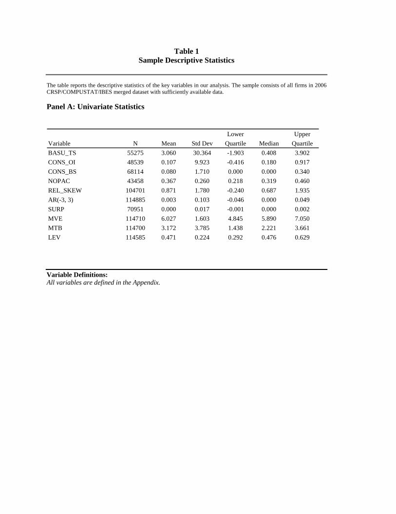
Table 1 Sample Descriptive Statistics
The table reports the descriptive statistics of the key variables in our analysis. The sample consists of all firms in 2006 CRSP/COMPUSTAT/IBES merged dataset with sufficiently available data.
Panel A: Univariate Statistics
Lower Upper
Variable N Mean Std Dev Quartile Median Quartile
BASU_TS 55275 3.060 30.364 -1.903 0.408 3.902
CONS_OI 48539 0.107 9.923 -0.416 0.180 0.917
CONS_BS 68114 0.080 1.710 0.000 0.000 0.340
NOPAC 43458 0.367 0.260 0.218 0.319 0.460
REL_SKEW 104701 0.871 1.780 -0.240 0.687 1.935
AR(-3, 3) 114885 0.003 0.103 -0.046 0.000 0.049
SURP 70951 0.000 0.017 -0.001 0.000 0.002
MVE 114710 6.027 1.603 4.845 5.890 7.050
MTB 114700 3.172 3.785 1.438 2.221 3.661
LEV 114585 0.471 0.224 0.292 0.476 0.629
Variable Definitions: All variables are defined in the Appendix.
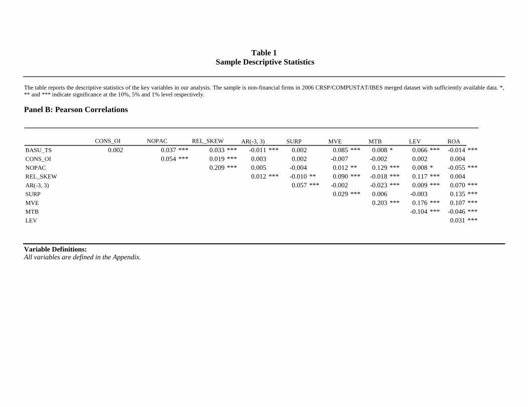
Table 1 Sample Descriptive Statistics
The table reports the descriptive statistics of the key variables in our analysis. The sample is non-financial firms in 2006 CRSP/COMPUSTAT/IBES merged dataset with sufficiently available data. *, ** and *** indicate significance at the 10%, 5% and 1% level respectively.
Panel B: Pearson Correlations
CONS_OI NOPAC REL_SKEW AR(-3, 3) SURP MVE MTB LEV ROA
BASU_TS 0.002 0.037 *** 0.033 *** -0.011 *** 0.002 0.085 *** 0.008 * 0.066 *** -0.014 ***CONS_OI 0.054 *** 0.019 *** 0.003 0.002 -0.007 -0.002 0.002 0.004NOPAC 0.209 *** 0.005 -0.004 0.012 ** 0.129 *** 0.008 * -0.055 ***REL_SKEW 0.012 *** -0.010 ** 0.090 *** -0.018 *** 0.117 *** 0.004AR(-3, 3) 0.057 *** -0.002 -0.023 *** 0.009 *** 0.070 ***SURP 0.029 *** 0.006 -0.003 0.135 ***MVE 0.203 *** 0.176 *** 0.107 ***MTB -0.104 *** -0.046 ***LEV 0.031 *** Variable Definitions: All variables are defined in the Appendix.
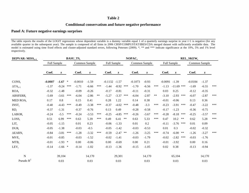
Table 2
Conditional conservatism and future negative performance
Panel A: Future negative earnings surprises
The table reports the results of the LOGIT regressions whose dependent variable is a dummy variable equal 1 of a quarterly earnings surprise in year t+1 is negative (for any available quarter in the subsequent year). The sample is composed of all firms in 2006 CRSP/COMPUSTAT/IBES/CDA merged dataset with sufficiently available data. The model is estimated using time fixed effects and cluster-adjusted standard errors, following Petersen (2009). *, ** and *** indicate significance at the 10%, 5% and 1% level respectively.
DEPVAR: MISS t+1
Coef. z Coef. z Coef. z Coef. z Coef. z Coef. z
CONSt -0.0007 -1.67 * -0.0010 -1.59 -0.1132 -1.57 -0.1073 -0.93 -0.0091 -1.39 -0.0184 -1.37
∆TAt+1 -1.37 -9.24 *** -1.71 -6.66 *** -1.44 -8.92 *** -1.70 -6.56 *** -1.13 -11.69 *** -1.69 -6.55 ***
ROAt -0.32 -1.48 -0.09 -0.26 -0.17 -0.81 -0.11 -0.31 0.03 0.25 -0.12 -0.35
ABSFERRt -5.69 -3.61 *** -6.04 -2.86 ** -5.27 -3.37 *** -6.04 -2.87 ** -3.10 -2.93 *** -6.07 -2.87 ***
MED ROAt 0.17 0.8 0.15 0.41 0.28 1.22 0.14 0.38 -0.01 -0.06 0.13 0.36
INSTt -0.40 -4.43 *** -0.49 -3.38 *** -0.37 -4.02 *** -0.48 -3.3 *** -0.23 -3.91 *** -0.47 -3.22 ***
RDt -0.37 -1.31 -0.37 -0.76 0.13 0.49 -0.28 -0.58 -0.17 -1.23 -0.36 -0.75
LABORt -0.24 -5.5 *** -0.24 -3.53 *** -0.25 -4.85 *** -0.26 -3.67 *** -0.28 -8.18 *** -0.25 -3.57 ***
LOSSt 0.51 6.99 *** 0.63 5.39 *** 0.49 6.41 ** 0.63 5.33 *** 0.47 10.2** 0.62 5.28 ***
LIT t -0.05 -1.15 0.01 0.23 -0.06 -1.33 0.01 0.2 -0.11 -3.76 *** 0.01 0.09
DURt -0.05 -1.38 -0.03 -0.5 -0.05 -1.42 -0.03 -0.53 0.01 0.3 -0.02-0.32
∆EARNt -0.84 -3.81 *** -1.28 -3.32 *** -0.59 -2.47 ** -1.26 -3.25 *** -0.74 -6.00 ** -1.26 -3.27 ***
MVE t -0.01 -0.85 -0.03 -1.52 -0.02 -1.41 -0.03 -1.79 -0.02 -2.82 *** -0.03 -1.76
MTB t -0.01 -1.93 * 0.00 -0.06 0.00 -0.69 0.00 0.21 -0.01 -3.92 0.00 0.16
LEVt -0.14 -1.66 * -0.14 -1.02 -0.13 -1.36 -0.15 -1.05 0.02 0.38 -0.13 -0.94
N 39,104 14,170 29,301 14,170 65,104 14,170
Pseudo R2 0.03 0.03 0.03 0.03 0.03 0.03
REL_SKEW t
Full Sample Common SampleFull Sample Common Sample Full Sample Common Sample
BASU_TSt NOPACt
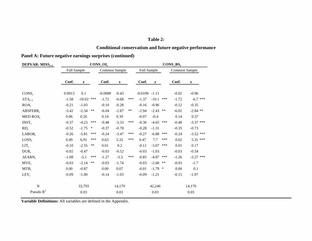
Table 2:
Conditional conservatism and future negative performance
Panel A: Future negative earnings surprises (continued)
DEPVAR: MISS t+1
Coef. z Coef. z Coef. z Coef. z
CONSt 0.0013 0.1 -0.0088 -0.43 -0.0109 -1.11 -0.02 -0.96
∆TAt+1 -1.58 -10.02 *** -1.72 -6.68 *** -1.37 -10.1 *** -1.72 -6.7 ***
ROAt -0.21 -1.03 -0.10 -0.28 -0.16 -0.96 -0.12 -0.35
ABSFERRt -3.42 -2.34 ** -6.04 -2.87 ** -2.94 -2.43 ** -6.02 -2.84 **
MED ROAt 0.06 0.26 0.14 0.39 -0.07 -0.4 0.14 0.37
INSTt -0.37 -4.23 *** -0.48 -3.33 *** -0.36 -4.65 *** -0.48 -3.37 ***
RDt -0.52 -1.75 * -0.37 -0.78 -0.28 -1.31 -0.35 -0.73
LABORt -0.26 -5.81 *** -0.24 -3.47 *** -0.27 -6.88 *** -0.24 -3.52 ***
LOSSt 0.49 6.91 *** 0.63 5.32 *** 0.47 7.7 *** 0.62 5.31 ***
LIT t -0.10 -2.55 ** 0.01 0.2 -0.11 -3.07 *** 0.01 0.17
DURt -0.02 -0.47 -0.03 -0.52 -0.03 -1.03 -0.03 -0.54
∆EARNt -1.08 -5.1 *** -1.27 -3.3 *** -0.85 -4.87 *** -1.26 -3.27 ***
MVE t -0.03 -2.14 ** -0.03 -1.74 -0.03 -2.68 ** -0.03 -1.7
MTB t 0.00 -0.87 0.00 0.07 -0.01 -1.79 * 0.00 0.1
LEV t -0.09 -1.00 -0.14 -1.03 -0.09 -1.21 -0.15 -1.07
N 33,793 14,170 42,246 14,170
Pseudo R2 0.03 0.03 0.03 0.03
CONS_OItFull Sample Common Sample
CONS_BSt
Full Sample Common Sample
Variable Definitions: All variables are defined in the Appendix.
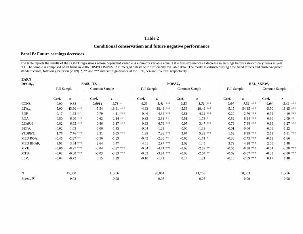
Table 2
Conditional conservatism and future negative performance
Panel B: Future earnings decreases
The table reports the results of the LOGIT regressions whose dependent variable is a dummy variable equal 1 if a firm experiences a decrease in earnings before extraordinary items in year t+1. The sample is composed of all firms in 2006 CRSP/COMPUSTAT merged dataset with sufficiently available data. The model is estimated using time fixed effects and cluster-adjusted standard errors, following Petersen (2009). *, ** and *** indicate significance at the 10%, 5% and 1% level respectively. EARN DECRt+1
Coef. z Coef. z Coef. z Coef. z Coef. z Coef. z
CONSt 0.00 -0.38 -0.0014 -1.76* -0.29 -5.41 *** -0.33 -3.71 *** -0.04 -7.32 *** -0.04 -3.49 ***
∆TAt+1 -5.00 -45.80 *** -5.54 -18.61 *** -4.83 -38.48 *** -5.53 -18.49 *** -5.15 -54.35 *** -5.50 -18.45 ***
EDF -0.17 -1.93 ** -0.79 -4.11 *** -0.46 -4.34 *** -0.81 -4.22*** -0.20 -2.70 *** -0.79 -4.10 ***
ROAt 0.80 6.90 *** 0.62 2.14 ** 0.32 2.61 ** 0.51 1.73 * 0.52 6.24 *** 0.60 2.09 **
∆EARNt 0.82 6.65 *** 0.86 3.17 *** 0.93 6.79 *** 0.97 3.47 *** 0.73 7.88 *** 0.89 3.27 ***
BETAt -0.02 -1.03 -0.06 -1.35 -0.04 -1.29 -0.06 -1.33 -0.01 -0.66 -0.06 -1.22
STDRETt 1.76 7.76 *** 2.51 5.05 *** 1.98 7.36 *** 2.67 5.32 *** 1.52 8.28 *** 2.52 5.11 ***
MED ROAt -0.45 -2.67 ** -0.56 -1.63 -0.45 -2.26 ** -0.60 -1.71 * -0.38 -2.75 *** -0.58 -1.66
MED BHARt 3.91 3.84 *** 2.64 1.47 4.01 2.97 *** 2.62 1.45 3.79 4.28 *** 2.66 1.48
MVEt -0.06 -8.27 *** -0.04 -2.87 *** -0.04 -4.74 *** -0.03 -2.59 ** -0.05 -8.58 *** -0.04 -2.98 ***
MTB t -0.02 -6.00 *** -0.03 -2.83 *** -0.02 -3.94 *** -0.03 -2.64 ** -0.02 -5.07 *** -0.03 -2.80 ***
LEV t -0.04 -0.72 0.15 1.29 -0.10 -1.41 0.14 1.21 -0.13 -2.69 *** 0.17 1.48
N 45,350 11,756 28,064 11,756 50,303 11,756
Pseudo R2 0.03 0.08 0.08 0.08 0.09 0.08
Full Sample Common Sample Full Sample Common Sample Full Sample Common Sample
BASU_TSt NOPACt REL_SKEW t
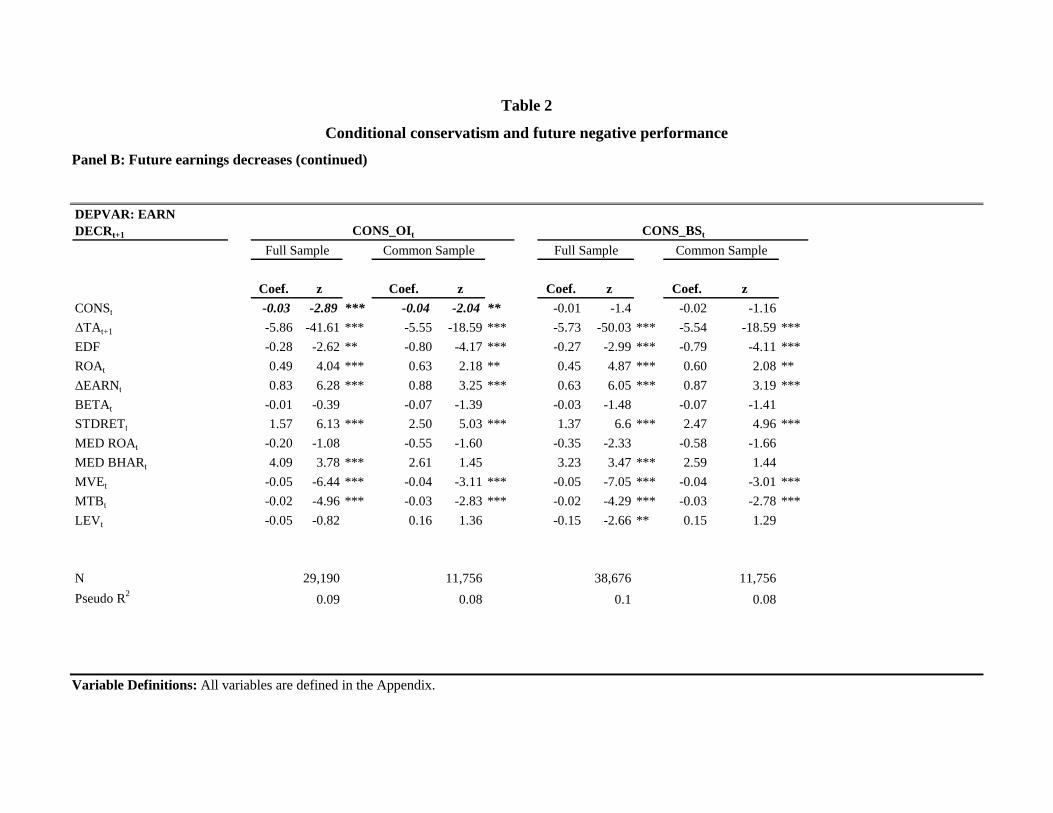
Table 2
Conditional conservatism and future negative performance
Panel B: Future earnings decreases (continued) DEPVAR: EARN DECRt+1
Coef. z Coef. z Coef. z Coef. z
CONSt -0.03 -2.89 *** -0.04 -2.04 ** -0.01 -1.4 -0.02 -1.16
∆TAt+1 -5.86 -41.61 *** -5.55 -18.59 *** -5.73 -50.03 *** -5.54 -18.59 ***
EDF -0.28 -2.62 ** -0.80 -4.17 *** -0.27 -2.99 *** -0.79 -4.11***
ROAt 0.49 4.04 *** 0.63 2.18 ** 0.45 4.87 *** 0.60 2.08 **
∆EARNt 0.83 6.28 *** 0.88 3.25 *** 0.63 6.05 *** 0.87 3.19 ***
BETAt -0.01 -0.39 -0.07 -1.39 -0.03 -1.48 -0.07 -1.41
STDRETt 1.57 6.13 *** 2.50 5.03 *** 1.37 6.6 *** 2.47 4.96 ***
MED ROAt -0.20 -1.08 -0.55 -1.60 -0.35 -2.33 -0.58 -1.66
MED BHARt 4.09 3.78 *** 2.61 1.45 3.23 3.47 *** 2.59 1.44
MVE t -0.05 -6.44 *** -0.04 -3.11 *** -0.05 -7.05 *** -0.04 -3.01 ***
MTB t -0.02 -4.96 *** -0.03 -2.83 *** -0.02 -4.29 *** -0.03 -2.78 ***
LEVt -0.05 -0.82 0.16 1.36 -0.15 -2.66 ** 0.15 1.29
N 29,190 11,756 38,676 11,756
Pseudo R2 0.09 0.08 0.1 0.08
Full Sample Common Sample Full Sample
CONS_OItCommon Sample
CONS_BSt
Variable Definitions: All variables are defined in the Appendix.
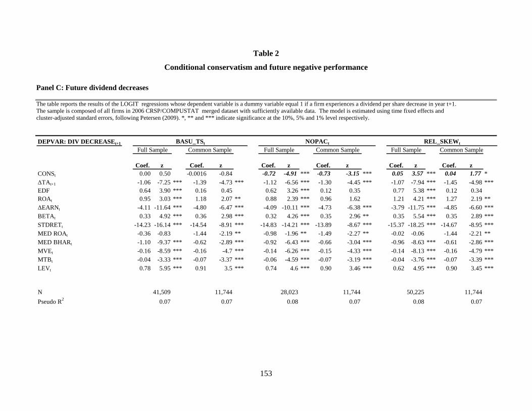
153
Table 2
Conditional conservatism and future negative performance Panel C: Future dividend decreases
The table reports the results of the LOGIT regressions whose dependent variable is a dummy variable equal 1 if a firm experiences a dividend per share decrease in year t+1. The sample is composed of all firms in 2006 CRSP/COMPUSTAT merged dataset with sufficiently available data. The model is estimated using time fixed effects and cluster-adjusted standard errors, following Petersen (2009). *, ** and *** indicate significance at the 10%, 5% and 1% level respectively.
DEPVAR: DIV DECREASE t+1
Coef. z Coef. z Coef. z Coef. z Coef. z Coef. zCONSt 0.00 0.50 -0.0016 -0.84 -0.72 -4.91 *** -0.73 -3.15 *** 0.05 3.57 *** 0.04 1.77 *∆TAt+1 -1.06 -7.25 *** -1.39 -4.73 *** -1.12 -6.56 *** -1.30 -4.45 *** -1.07 -7.94 *** -1.45 -4.98 ***EDF 0.64 3.90 *** 0.16 0.45 0.62 3.26 *** 0.12 0.35 0.77 5.38 *** 0.12 0.34ROAt 0.95 3.03 *** 1.18 2.07 ** 0.88 2.39 *** 0.96 1.62 1.21 4.21 *** 1.27 2.19 **∆EARNt -4.11 -11.64 *** -4.80 -6.47 *** -4.09 -10.11 *** -4.73 -6.38*** -3.79 -11.75 *** -4.85 -6.60 ***BETAt 0.33 4.92 *** 0.36 2.98 *** 0.32 4.26 *** 0.35 2.96 ** 0.35 5.54*** 0.35 2.89 ***STDRETt -14.23 -16.14 *** -14.54 -8.91 *** -14.83 -14.21 *** -13.89 -8.67 *** -15.37 -18.25 *** -14.67 -8.95 ***MED ROAt -0.36 -0.83 -1.44 -2.19 ** -0.98 -1.96 ** -1.49 -2.27 ** -0.02-0.06 -1.44 -2.21 **MED BHARt -1.10 -9.37 *** -0.62 -2.89 *** -0.92 -6.43 *** -0.66 -3.04 *** -0.96 -8.63 *** -0.61 -2.86 ***MVE t -0.16 -8.59 *** -0.16 -4.7 *** -0.14 -6.26 *** -0.15 -4.33 *** -0.14 -8.13 *** -0.16 -4.79 ***MTB t -0.04 -3.33 *** -0.07 -3.37 *** -0.06 -4.59 *** -0.07 -3.19 *** -0.04 -3.76 *** -0.07 -3.39 ***LEVt 0.78 5.95 *** 0.91 3.5 *** 0.74 4.6 *** 0.90 3.46 *** 0.62 4.95 *** 0.90 3.45 ***
N 41,509 11,744 28,023 11,744 50,225 11,744
Pseudo R2 0.07 0.07 0.08 0.07 0.08 0.07
Full Sample Common SampleBASU_TSt NOPACt REL_SKEW t
Full Sample Common Sample Full Sample Common Sample
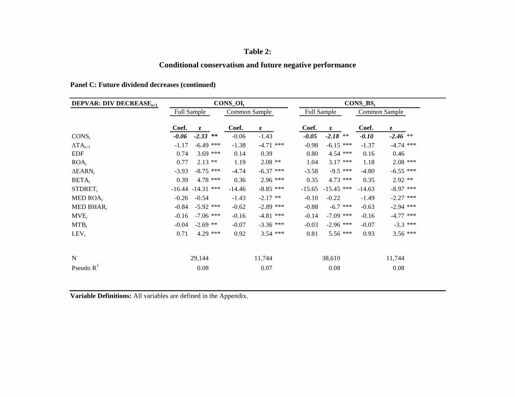
Table 2:
Conditional conservatism and future negative performance Panel C: Future dividend decreases (continued) DEPVAR: DIV DECREASE t+1
Coef. z Coef. z Coef. z Coef. zCONSt -0.06 -2.33 ** -0.06 -1.43 -0.05 -2.18 ** -0.10 -2.46 **∆TAt+1 -1.17 -6.49 *** -1.38 -4.71 *** -0.98 -6.15 *** -1.37 -4.74 ***EDF 0.74 3.69 *** 0.14 0.39 0.80 4.54 *** 0.16 0.46ROAt 0.77 2.13 ** 1.19 2.08 ** 1.04 3.17 *** 1.18 2.08 ***∆EARNt -3.93 -8.75 *** -4.74 -6.37 *** -3.58 -9.5 *** -4.80 -6.55 ***BETAt 0.39 4.78 *** 0.36 2.96 *** 0.35 4.73 *** 0.35 2.92 **STDRETt -16.44 -14.31 *** -14.46 -8.85 *** -15.65 -15.45 *** -14.63 -8.97 ***MED ROAt -0.26 -0.54 -1.43 -2.17 ** -0.10 -0.22 -1.49 -2.27 ***MED BHARt -0.84 -5.92 *** -0.62 -2.89 *** -0.88 -6.7 *** -0.63 -2.94 ***MVE t -0.16 -7.06 *** -0.16 -4.81 *** -0.14 -7.09 *** -0.16 -4.77 ***MTB t -0.04 -2.69 ** -0.07 -3.36 *** -0.03 -2.96 *** -0.07 -3.3 ***LEV t 0.71 4.29 *** 0.92 3.54 *** 0.81 5.56 *** 0.93 3.56 ***
N 29,144 11,744 38,610 11,744
Pseudo R2 0.08 0.07 0.08 0.08
Full Sample Common Sample Full SampleCONS_OIt
Common SampleCONS_BSt
Variable Definitions: All variables are defined in the Appendix.
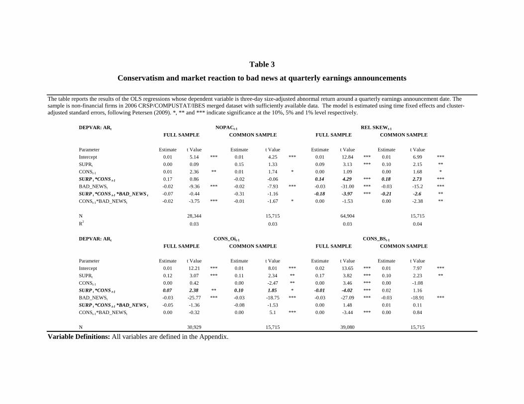
Table 3
Conservatism and market reaction to bad news at quarterly earnings announcements
The table reports the results of the OLS regressions whose dependent variable is three-day size-adjusted abnormal return around a quarterly earnings announcement date. The sample is non-financial firms in 2006 CRSP/COMPUSTAT/IBES merged dataset with sufficiently available data. The model is estimated using time fixed effects and cluster-adjusted standard errors, following Petersen (2009). *, ** and *** indicate significance at the 10%, 5% and 1% level respectively.
DEPVAR: AR t
Parameter Estimate t Value Estimate t Value Estimate t Value Estimate t Value
Intercept 0.01 5.14 *** 0.01 4.25 *** 0.01 12.84 *** 0.01 6.99 ***
SUPRt 0.00 0.09 0.15 1.33 0.09 3.13 *** 0.10 2.15 **
CONSt-1 0.01 2.36 ** 0.01 1.74 * 0.00 1.09 0.00 1.68 *
SURPt *CONS t-1 0.17 0.86 -0.02 -0.06 0.14 4.29 *** 0.18 2.73 ***
BAD_NEWSt -0.02 -9.36 *** -0.02 -7.93 *** -0.03 -31.00 *** -0.03 -15.2 ***
SURPt *CONS t-1 *BAD_NEWS t -0.07 -0.44 -0.31 -1.16 -0.18 -3.97 *** -0.21 -2.6 **
CONSt-1*BAD_NEWSt -0.02 -3.75 *** -0.01 -1.67 * 0.00 -1.53 0.00 -2.38 **
N 28,344 15,715 64,904 15,715
R20.03 0.03 0.03 0.04
DEPVAR: AR t
Parameter Estimate t Value Estimate t Value Estimate t Value Estimate t Value
Intercept 0.01 12.21 *** 0.01 8.01 *** 0.02 13.65 *** 0.01 7.97 ***
SUPRt 0.12 3.07 *** 0.11 2.34 ** 0.17 3.82 *** 0.10 2.23 **
CONSt-1 0.00 0.42 0.00 -2.47 ** 0.00 3.46 *** 0.00 -1.08
SURPt *CONS t-1 0.07 2.38 ** 0.10 1.85 * -0.01 -4.02 *** 0.02 1.16
BAD_NEWSt -0.03 -25.77 *** -0.03 -18.75 *** -0.03 -27.09 *** -0.03 -18.91 ***
SURPt *CONS t-1 *BAD_NEWS t -0.05 -1.36 -0.08 -1.53 0.00 1.48 0.01 0.11
CONSt-1*BAD_NEWSt 0.00 -0.32 0.00 5.1 *** 0.00 -3.44 *** 0.00 0.84
N 30,929 15,715 39,080 15,715
FULL SAMPLE COMMON SAMPLE FULL SAMPLE COMMON SAMPLE
NOPACt-1 REL SKEW t-1
CONS_Oit-1FULL SAMPLE COMMON SAMPLE
CONS_BSt-1
FULL SAMPLE COMMON SAMPLE
Variable Definitions: All variables are defined in the Appendix.

Chapter V
Conclusions
Although conservatism has been widely viewed as a mechanism to enhance debt
contract efficiency, we know little about whether a firm commit to its pre-contracting
level of conservatism and the factors that affect this commitment. My first essay
provides evidence that firms are, on average, committed to their pre-borrowing
conservatism level and, therefore, that conservatism is indeed an effective tool to enhance
debt-contract efficiency. This research also provides debt holders with implication that
firms with a high expected cost of breaching covenants will have incentives to deviate
from the pre-contracting level of conservatism after borrowing.
The evidence in the second essay suggests the financial market reforms may be
another channel through which countries may influence firms’ financial reporting.
Contrary to changes in regulations regarding disclosure and auditing rules, which directly
affect firms’ accounting quality, our evidence suggests that an increase in lending market
competition may indirectly affect financial reporting by improving firms’ incentive to
produce higher quality statements. The evidence also provides a new perspective to the
potential effects of greater credit market competition on lending relationships and the
supply of credit to informationally-opaque firms. Our evidence suggests that firms’
inherent opaqueness may not be completely fixed.
Our findings from the third essay have important implications for accounting
regulators and policy-makers. First, we explicitly establish that conditional conservatism has
some, albeit small, informational benefits in the form of reduced probability of future bad
accounting news. Our finding of some positive valuation effects for conservatism suggests
157
that the market rewards these properties of conservatism somewhat, albeit not in great degree.
Thus, considering these effects is also important in the process of convergence of the U.S.
GAAP to IFRS. IFRS is also influenced by the fair value principle (Leone, 2007), and some
have argued that abolishing conservatism will result in the loss of important benefits of
conservatism (Watts, 2003).