Embed Size (px)
Citation preview
ESSAYS OF CAPITAL STRUCTURE, RISK MANAGEMENT, AND OPTIONS
ON INDEX FUTURES
by
TZU TAI
A dissertation submitted to the
Graduate School-Newark
Rutgers, The State University of New Jersey
in partial fulfillment of requirements
for the degree of
Doctor of Philosophy
Graduate Program in Management
written under the direction of
Professor Cheng-Few Lee
and approved by
________________________________
________________________________
________________________________
________________________________
Newark, New Jersey
May, 2014

© 2014
TZU TAI
ALL RIGHTS RESERVED
ii
ABSTRACT OF THE DISSERTATION
Essays of Capital Structure, Risk Management, and Options on Index Futures
By Tzu Tai
Thesis director: Professor Cheng-Few Lee
This dissertation includes the following three essays involved in the joint
determination of capital structure and stock rate of return, fair deposit insurance premium
estimation, and the prediction of implied volatility of options on index futures.
The first essay identifies the joint determinants of capital structure and stock returns
by using three alternative approaches to deal with the measurement error-in-variable
problem. The main contribution of this essay is the comprehensive confirmation on
theories in corporate finance. The empirical results from the structural equation modeling
(SEM) with confirmatory factor analysis (CFA) show that stock returns, asset structure,
growth, industry classification, uniqueness, volatility and financial rating, profitability,
government financial policy, and managerial entrenchment are main factors of capital
structure in either market- or book- value basis. Finally, the results in robustness test by
using the Multiple Indicators and Multiple Causes (MIMIC) model and the two-stage,
least square (2SLS) method show the necessity and importance of latent attributes to
iii
describe the trade-off between the financial distress and agency costs in capital structure
choice.
In the second essay, we use the structural model in terms of the Stair Tree model and
barrier option to evaluate the fair deposit insurance premium in accordance with the
constraints of the deposit insurance contracts and the consideration of bankruptcy costs.
The simulation results suggest that insurers should adopt a forbearance policy instead of a
strict policy for closure regulation to avoid losses from bankruptcy costs. An appropriate
deposit insurance premium can alleviate potential moral hazard problems caused by a
forbearance policy.
In the third essay, we use two alternative approaches, time-series and cross-sectional
analysis and constant elasticity of variance (CEV) model, to give different perspective of
forecasting implied volatility. We use call options on the S&P 500 index futures expired
within 2010 to 2013 to do the empirical work. The abnormal returns in our trading
strategy indicate the market of options on index futures may be inefficient. The CEV
model performs better than Black model because it can generalize implied volatility
surface as a function of asset price.

iv
DEDICATION
This dissertation is dedicated to my family, Chun-Ping Hilton Tai, Li-Chin Susan
Peng, Jui-Hung Ray Tai, and Jui-Chuan Lewis Tai.

v
ACKNOWLEDGEMENT
I would like to express my deepest gratitude and appreciation to my dissertation
advisor, Professor Cheng-Few Lee, who has provided me valuable guidance, full support
and strong encouragement all along my Ph.D. studies. I would also like to express my
very great appreciation to the committee members, Professor Ren-Raw Chen, Professor
Ben Sopranzetti, and Professor Zhaodong (Ken) Zhong, for insightful advice and warm
encouragement.
I owe thanks to my dearest friends, especially to Victoria Chiu, Yuna Heo, Hua-Yao
Wu, Wei-Hao Huang, Hong-Yi Chen, Chin-Hsun Wang and Marcus Hong; your warm
friendship and academic support will always be cherished.
Finally, I would like to express my gratitude to my family for their continuous
support and encourage throughout my studies. From the bottom of my heart, thank you
all for making my achievement possible.

vi
Table of Contents
2.1 Introduction .......................................................................................................... 7
2.2 Determinants of Capital Structure and Data ...................................................... 12
2.2.1 Determinants of Capital Structure .............................................................. 12
2.2.1.1 Firm characteristics ......................................................................... 12
2.2.1.2 Macroeconomic factors ................................................................... 20
2.2.1.3 Manager character ........................................................................... 22
2.2.2 Joint Determinants of Capital Structure and Stock Rate of Return ............ 24
2.2.3 Data ............................................................................................................. 29
2.3 Methodologies and LISREL System .................................................................. 31
2.3.1 SEM Approach ........................................................................................... 31
2.3.2 Illustration of SEM Approach in LISREL System ..................................... 33
2.3.3 Multiple Indicators Multiple Causes (MIMIC) Model ............................... 38
2.3.4 Confirmatory Factor Analysis (CFA) ......................................................... 41
2.4 Empirical Analysis ............................................................................................. 43
2.4.1 Determinants of Capital Structure by SEM with CFA ............................... 44
2.4.2 Determinants of Capital Structure by MIMIC Model ................................ 51
ESSAYS OF CAPITAL STRUCTURE, RISK MANAGEMENT, AND OPTIONS ON
INDEX FUTURES ........................................................................................................ ii
ABSTRACT OF THE DISSERTATION ....................................................................... ii
DEDICATION .............................................................................................................. iv
ACKNOWLEDGEMENT ............................................................................................. v
Table of Contents .......................................................................................................... vi
Lists of Tables ............................................................................................................... ix
Lists of Figures ............................................................................................................. xi
CHAPTER 1 .................................................................................................................. 1
Introduction .................................................................................................................... 1
CHAPTER 2 .................................................................................................................. 7
The Joint Determinants of Capital Structure and Stock Rate of Return: A LISREL
Model Approach............................................................................................................. 7
vii
2.4.3 Joint Determinants of Capital Structure and Stock Returns by SEM with
CFA ..................................................................................................................... 55
2.4.4 Robustness for Joint Determinants of Capital Structure and Stock Returns65
2.5 Conclusion .......................................................................................................... 70
Appendix 2.A: Codes of Structure Equation Modeling (SEM) in LISREL System 73
Appendix 2.B: Codes of MIMIC Model in LISREL System ................................... 75
3.1 Introduction ........................................................................................................ 76
3.2 The Methodology ............................................................................................... 82
3.3 Simulation Results.............................................................................................. 91
3.3.1 Parameters analysis ..................................................................................... 91
3.3.2 Moral Hazard Problem ............................................................................... 95
3.4 Conclusion .......................................................................................................... 96
4.1 Introduction ........................................................................................................ 98
4.2 Literature Review ............................................................................................. 102
4.2.1 Black-Scholes-Merton Option Pricing Model (BSM) and CEV Model... 102
4.2.2 Time-Varying Volatility and Time Series Analysis ................................. 112
4.3 Data and Methodology ..................................................................................... 114
4.3.1 Data ........................................................................................................... 114
4.3.2 Methodology ............................................................................................. 117
4.3.2.1 Estimating BSM IV ...................................................................... 117
4.3.2.2 Forecasting IV by Cross-Sectional and Time-Series Analysis ..... 122
4.3.2.2.1 Time-Series Analysis ............................................................ 122
4.3.2.2.1 Cross-sectional Predictive Regression Model ...................... 125
4.3.2.3 Forecasting IV by CEV Model ..................................................... 129
CHAPTER 3 ................................................................................................................ 76
Pricing Fair Deposit Insurance: Structural Model Approach ....................................... 76
CHAPTER 4 ................................................................................................................ 98
Forecasting Implied Volatilities for Options on Index Futures: Time Series and
Cross-Sectional Analysis versus Constant Elasticity of Variance (CEV) Model ........ 98
viii
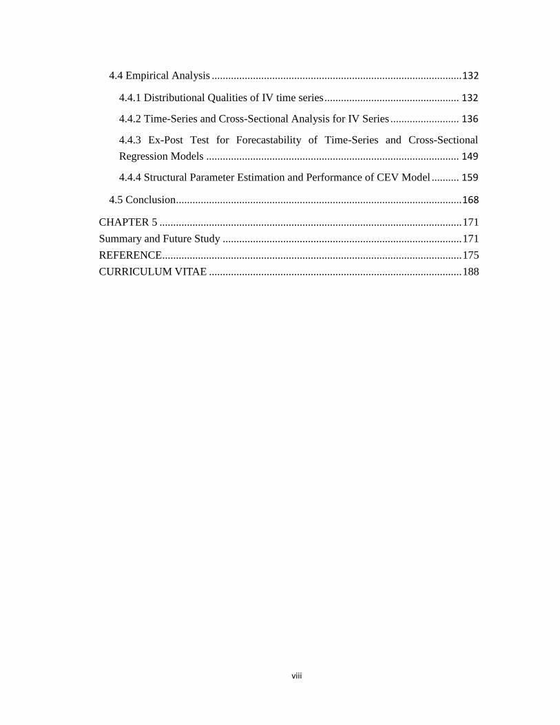
4.4 Empirical Analysis ........................................................................................... 132
4.4.1 Distributional Qualities of IV time series ................................................. 132
4.4.2 Time-Series and Cross-Sectional Analysis for IV Series ......................... 136
4.4.3 Ex-Post Test for Forecastability of Time-Series and Cross-Sectional
Regression Models ............................................................................................ 149
4.4.4 Structural Parameter Estimation and Performance of CEV Model .......... 159
4.5 Conclusion ........................................................................................................ 168
CHAPTER 5 .............................................................................................................. 171
Summary and Future Study ....................................................................................... 171
REFERENCE ............................................................................................................. 175
CURRICULUM VITAE ............................................................................................ 188
ix
Lists of Tables
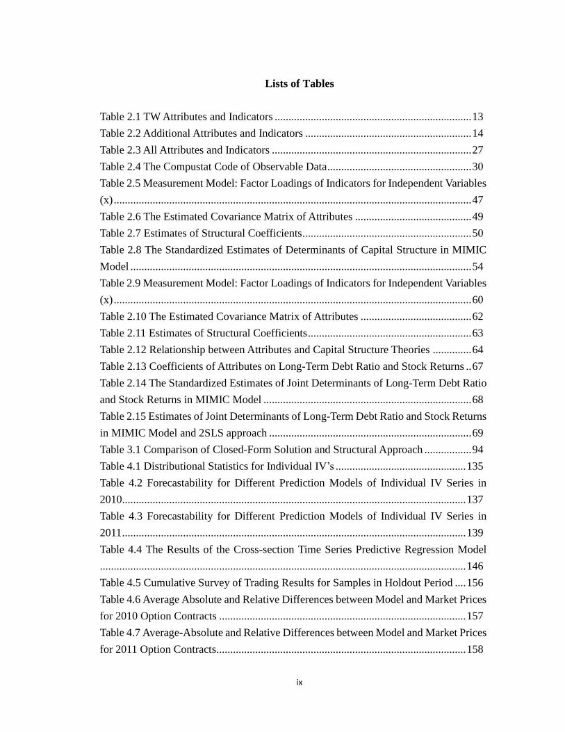
Table 2.1 TW Attributes and Indicators ....................................................................... 13
Table 2.2 Additional Attributes and Indicators ............................................................ 14
Table 2.3 All Attributes and Indicators ........................................................................ 27
Table 2.4 The Compustat Code of Observable Data .................................................... 30
Table 2.5 Measurement Model: Factor Loadings of Indicators for Independent Variables
(x) ................................................................................................................................. 47
Table 2.6 The Estimated Covariance Matrix of Attributes .......................................... 49
Table 2.7 Estimates of Structural Coefficients ............................................................. 50
Table 2.8 The Standardized Estimates of Determinants of Capital Structure in MIMIC
Model ........................................................................................................................... 54
Table 2.9 Measurement Model: Factor Loadings of Indicators for Independent Variables
(x) ................................................................................................................................. 60
Table 2.10 The Estimated Covariance Matrix of Attributes ........................................ 62
Table 2.11 Estimates of Structural Coefficients ........................................................... 63
Table 2.12 Relationship between Attributes and Capital Structure Theories .............. 64
Table 2.13 Coefficients of Attributes on Long-Term Debt Ratio and Stock Returns .. 67
Table 2.14 The Standardized Estimates of Joint Determinants of Long-Term Debt Ratio
and Stock Returns in MIMIC Model ........................................................................... 68
Table 2.15 Estimates of Joint Determinants of Long-Term Debt Ratio and Stock Returns
in MIMIC Model and 2SLS approach ......................................................................... 69
Table 3.1 Comparison of Closed-Form Solution and Structural Approach ................. 94
Table 4.1 Distributional Statistics for Individual IV’s ............................................... 135
Table 4.2 Forecastability for Different Prediction Models of Individual IV Series in
2010............................................................................................................................ 137
Table 4.3 Forecastability for Different Prediction Models of Individual IV Series in
2011 ............................................................................................................................ 139
Table 4.4 The Results of the Cross-section Time Series Predictive Regression Model
.................................................................................................................................... 146
Table 4.5 Cumulative Survey of Trading Results for Samples in Holdout Period .... 156
Table 4.6 Average Absolute and Relative Differences between Model and Market Prices
for 2010 Option Contracts ......................................................................................... 157
Table 4.7 Average-Absolute and Relative Differences between Model and Market Prices
for 2011 Option Contracts .......................................................................................... 158

x
Table 4.8 Average Daily and Total Number of Observations in Each Group ............ 160
Table 4.9 Initial Parameters of CEV Model for Estimation Procedure ..................... 161
Table 4.10 Total Number of Observations and Trading Days in Each Group ........... 163
Table 4.11 Average Daily Parameters of In-Sample .................................................. 165
Table 4.12 AveAPE Performance for In-Sample-Fitness ........................................... 165
Table 4.13 AveAPE Performance for Out-of-Sample ................................................ 167
xi
Lists of Figures
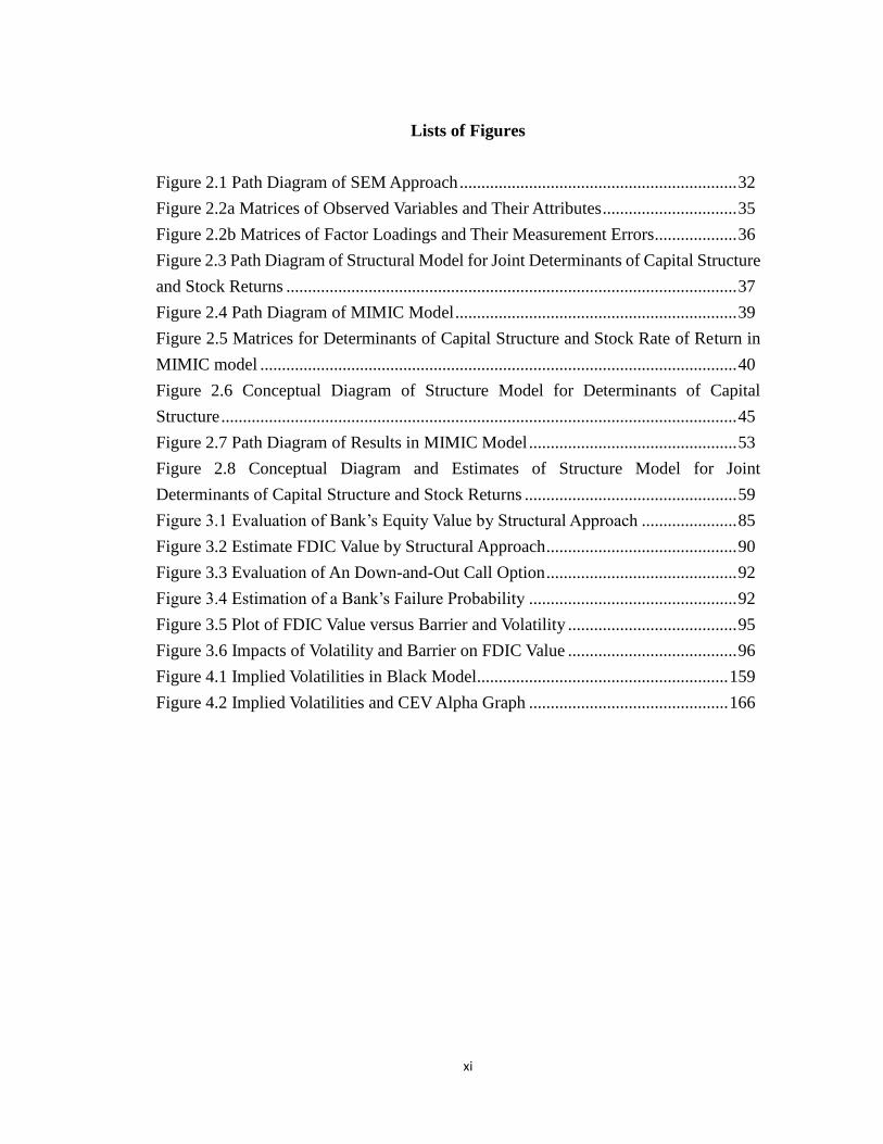
Figure 2.1 Path Diagram of SEM Approach ................................................................ 32
Figure 2.2a Matrices of Observed Variables and Their Attributes ............................... 35
Figure 2.2b Matrices of Factor Loadings and Their Measurement Errors................... 36
Figure 2.3 Path Diagram of Structural Model for Joint Determinants of Capital Structure
and Stock Returns ........................................................................................................ 37
Figure 2.4 Path Diagram of MIMIC Model ................................................................. 39
Figure 2.5 Matrices for Determinants of Capital Structure and Stock Rate of Return in
MIMIC model .............................................................................................................. 40
Figure 2.6 Conceptual Diagram of Structure Model for Determinants of Capital
Structure ....................................................................................................................... 45
Figure 2.7 Path Diagram of Results in MIMIC Model ................................................ 53
Figure 2.8 Conceptual Diagram and Estimates of Structure Model for Joint
Determinants of Capital Structure and Stock Returns ................................................. 59
Figure 3.1 Evaluation of Bank’s Equity Value by Structural Approach ...................... 85
Figure 3.2 Estimate FDIC Value by Structural Approach ............................................ 90
Figure 3.3 Evaluation of An Down-and-Out Call Option ............................................ 92
Figure 3.4 Estimation of a Bank’s Failure Probability ................................................ 92
Figure 3.5 Plot of FDIC Value versus Barrier and Volatility ....................................... 95
Figure 3.6 Impacts of Volatility and Barrier on FDIC Value ....................................... 96
Figure 4.1 Implied Volatilities in Black Model .......................................................... 159
Figure 4.2 Implied Volatilities and CEV Alpha Graph .............................................. 166
1
CHAPTER 1
Introduction
This thesis investigates three important issues in finance: capital structure, deposit
insurance, and options on index future. The first essay investigates the joint determination
of capital structure and stock rate of return by using LISREL model to reduce
measurement error-in-variable problem. The second essay examines fair deposit
insurance premium in accordance with the restrictions of insurance contracts by the
structural model approach in terms of the Stair Tree model and the barrier option model.
In the third essay, we forecast the implied volatility of options on index futures by using
either time-series and cross-sectional analysis or constant elasticity of variance (CEV)
model.
Most previous studies in capital structure investigate unobservable theoretical
variables which affect the capital structure of a firm. However, the use of observed
accounting variables as theoretical explanatory latent variables will cause measurement
error-in-variable problems during the analysis of the factors of capital structure.
Therefore, in the first essay, we employ LISREL approach to solve the measurement
errors problems in the analysis of the determinants of capital structure. This is the
2
comprehensive study to confirm the trade-off theory between the financial distress and
agency costs, pecking order theory, and signaling theory with asymmetric information in
corporate finance literature. The purpose of this essay is to investigate whether the factors
of capital structure that are related to the firm, manager, and macroeconomic
characteristics are consistent with theories in previous literature. This essay also aims at
the interrelation between capital structure and stock rate of returns. First, we employ
structural equation modeling (SEM) with confirmatory factor analysis (CFA) approach to
classify the observed variables into several groups (attributes) to verify these theories.
Then, we can test endogenous supply relationship between short-term public debt and
private debt through macroeconomic factor analysis. Finally, Dittmar’s and Thakor’s
(2007) “managerial investment autonomy” also can be verified via simultaneous
equations of capital structure and stock returns. Our empirical results show that there are
two significant theoretical attributes on the decision of capital structure. However, all
attributes become significant determinants of capital structure and stock returns. The
evidence shows that the interaction of a firm’s leverage and its stock price should be
necessarily considered in capital structure research. In addition, the results in robustness
test by using the Multiple Indicators and Multiple Causes (MIMIC) model and the
two-stage, least square (2SLS) method show the necessity and importance of latent

3
attributes to describe the trade-off between the financial distress and agency costs in
capital structure choice. Therefore, we claim that SEM with CFA approach is preceded by
adding latent attributes of capital structure and solving measurement error-in-variable
problem.
Since subprime mortgage crises broke out in August, 2007, pricing fair deposit
insurance premium became an important issue again because the panic of depositors
arose from many financial institutions with financial and liquidity distress. The Federal
Deposit Insurance Corporation (FDIC) should adjust the proper deposit insurance
premium as the trade-off that offsets the costs of bailout plans and the costs of taking
over the deposit account business and partial debt once the financial institutions are
announced bankruptcies. Based on the critical role that insurance deposit risk plays in
financial institutions, the purpose of the second essay is to investigate the pricing fair
value of deposit insurance. The most studies estimate fair-market FDIC insurance
premium by a structural approach, which typically bases the firm’s asset and the volatility
of its asset on its equity price. However, the structural models used in previous studies
neglects the restrictions of the deposit insurance contacts. In hence, the second essay
proposes the structural model approach in terms of the barrier option model and the Stair
Tree model to deal with bankruptcy costs, the limited indemnification for depositors,
4
discretely monitoring banks’ situations and the adjustment of the insurance premium in
different financial institution based on a risk-based assessment system. We are then able
to build a fair insurance premium system and calculate the reasonable implied barrier
critical points to determine whether FDIC’s supervisory policy is strict or forbearing. The
simulation results suggest that insurers should adopt a forbearance policy instead of a
strict policy for closure regulation to avoid losses from bankruptcy costs. In addition, an
appropriate deposit insurance premium can alleviate potential moral hazard problems
caused by a forbearance policy.
Forecasting volatility is crucial to risk management and financial decision for future
uncertainty. The third essay aims to improve the ability to forecast the implied volatility
(IV) for options on index futures. We use option prices instead of relying on the past
behavior of asset prices to infer volatility expectations of underlying assets. The two
alternative approaches used in this paper give different perspective of estimating IV. The
cross-sectional time series analysis focuses on the dynamic behavior of volatility in each
option contracts. The predicted IV obtained from the time series model is the estimated
conditional volatility based on the information of IV extracted from Black model.
Although the estimated IVs in a time series model vary across option contracts, this kind
of model can seize the specification of time-vary characteristic that links ex post
5
volatility to ex ante volatility for each option contract. In addition, cross-sectional
analysis can capture other trading behaviors such as week effect and in- /out- of the
money effect. On the other hand, CEV model generalizes implied volatility surface as a
function of asset price. It can reduce more computational and implementation costs rather
than the complex models such as jump-diffusion stochastic volatility models because
there is only one more variable compared with Black model. Although the constant
estimated IV for each trading day may cause low forecast power of whole option contacts,
it is more reasonable that the IVs of underlying assets are independent of different strike
prices and times to expiration. The empirical results show that volatility changes are
predictable by using cross-sectional time series analysis and CEV model. The prediction
power of these two methods can draw specific implications as to how Black model might
be misspecified. In addition, the abnormal returns based on our trading strategy with the
consideration of transaction costs imply the inefficiency of options on index future
market.
The structure of this thesis is as follows. Chapter 2 is the first essay entitled “The
Joint Determinants of Capital Structure and Stock Rate of Return: A LISREL Model
Approach”. The second essay entitled “Pricing Fair Deposit Insurance: Structural Model
Approach” is described in Chapter 3. Chapter 4 is the third essay entitled “Forecasting

6
Implied Volatilities for Options on Index Futures: Time Series and Cross-Sectional
Analysis versus Constant Elasticity of Variance (CEV) Model”. Finally, Chapter 5
represents the conclusions and future study of these three essays.
7
CHAPTER 2
The Joint Determinants of Capital Structure and Stock Rate of Return: A LISREL
Model Approach
2.1 Introduction
The abundant studies in capital structure indicate that the optimal capital structure is
determined by a trade-off related to the marginal costs from financial distress and agency
problem, the benefits from tax shields, and reduction of free cash flow problems
(Grossman and Hart, 1982; Stulz and Johnson, 1985; Rajan and Zingales, 1995; Parrino
and Weisbach, 1999; Frank and Goyal, 2009). Fischer, Heinkel, and Zechner (1989)
develop a dynamic capital structural model without the setting of static leverage measures.
The empirical results in Fisher et al. (1989) support their theoretical framework that the
debt-to-equity ratio changed over time and therefore the firm’s financing decisions should
be analyzed under a dynamic setting framework. However, Leary and Roberts (2005)
claim that the adjustment costs of rebalancing capital structure are of importance in the
determinants of capital structure. Although the debt-to-equity ratio should follow a
dynamic capital structural framework, firms may not change their leverage ratios
frequently because of the adjustment costs. Therefore, a firm’s capital structure is not

8
changed over time if its leverage ratio stays within an optimal range. To capture the
determinants of capital structure within an optimal range of leverage ratio, the traditional
linear regression analysis may be not a suitable methodology to investigate capital
structure because the estimates of independent variables (determinants of capital structure)
directly affect the dependent variables (leverage ratio) in regression. In addition,
regression analysis has difficulty in usage of dummy variables to control the size of the
effects of independent factor variables on leverage ratio within optimal range since the
optimal leverage ranges of firms are various and have difficulty in designing the critical
value of dummy variables.
Moreover, in previous research in capital structure, many models are derived based
on theoretical variables; however, these variables are often unobservable in the real world.
Therefore, many studies use the accounting items from the financial statements as proxies
to substitute for the theoretically derived variables. In the regression analysis, the
estimated parameters from accounting items as proxies for unobservable theoretical
attributes would cause some problems. First, there are measurement errors between the
observable proxies and latent variables1. According to the previous theoretical literature
1 In statistics, latent variables (as opposed to observable variables), are variables that are not directly
observed but are rather inferred (through a mathematical model) from other variables that are observed
(directly measured).

9
in corporate finance, a theoretical variable can be formed with either one or several
observed variables as a proxy. But there is no clear rule to allocate the unique weights of
observable variables as the perfect proxy of a latent variable. Second, because of
unobservable attributes to capital structure choice, researchers can choose different
accounting items to measure the same attribute in accordance with the various capital
structure theory and the their bias economic interpretation. The use of these observed
variables as theoretical explanatory latent variables in both cases will cause
error-in-variable problems. Joreskog (1977), Joreskog and Sorbom (1981, 1989) and
Jorekog and Goldberger (1975) first develop the structure equation modeling (hereafter
called SEM) to analyze the relationship between the observed variables as the indicators
and the latent variables as the attributes of the capital structure choice.
Since Titman and Wessels (1988) (hereafter called TW) first utilize LISREL system
to analyze the determinants of capital structure choice based on a structural equation
modeling (SEM) framework, Chang, Lee and Lee (2009) and Yang, Lee, Gu and Lee
(2010) extend the empirical work on capital structure choice and obtain more convincing
results. These papers employ structural equation modeling (SEM) in LISREL system to
solve the measurement errors problems in the analysis of the determinants of capital
structure and to find the important factors consistent with capital structure theories.

10
Although TW initially apply SEM to analyze the factors of capital structure choice, their
results are insignificant and poor to explain capital structure theories. Maddala and
Nimalendran (1996) point out the problematic model specification as the reason for TW’s
poor finding and propose a Multiple Indicators and Multiple Causes (hereafter called
MIMIC) model to improve the results. Chang et al. (2009) reproduce TW’s research on
determinants of capital structure choice but use MIMIC model to compare the results
with TW’s. They state that the results show the significant effects on capital structure in a
simultaneous cause-effect framework rather than in SEM framework. Later, Yang et al.
(2010) incorporate the stock returns with the research on capital structure choice and
utilize structural equation modeling (SEM) with confirmatory factor analysis (CFA)
approach to solve the simultaneous equations with latent determinants of capital structure.
They assert that a firm’s capital structure and its stock return are correlated and should be
decided simultaneously. Their results are mainly same as TW’s finding; moreover, they
also find that the stock returns as a main factors of capital structure choice.
The purpose of this paper is to investigate whether the factors of capital structure
that are related to the firm, manager, and macroeconomic characteristics are consistent
with theories in previous literature. This essay also aims at the interrelation between
capital structure and stock rate of returns. This is the comprehensive study to confirm the
11
trade-off theory between the financial distress and agency costs, pecking order theory,
and signaling theory with asymmetric information in corporate finance literature. We
employ SEM with CFA approach to classify the observed variables into several groups
(attributes) to verify these theories. Then, we can test McDonald’s (1983) endogenous
supply relationship between short-term public debt and private debt through
macroeconomic factors. Finally, Dittmar’s and Thakor’s (2007) “managerial investment
autonomy” also can be verified via simultaneous equations of capital structure and stock
returns. The MIMIC model and 2SLS method are used in this paper for robust test. The
results of robust test show the necessity and importance of the classifications of variables.
Therefore, we claim that SEM with CFA approach is preceded by adding latent attributes
of capital structure and solving measurement error-in-variable problem.
This paper is organized as follows. In section 2.2, we discuss the accounting items,
macroeconomic factors, and manager characteristics used as proxies of the factors of
capital structure. The additional factors of stock prices are also considered in the
investigation of joint determinants of capital structure and stock rate of return. Then, the
description of sample period and data sources is included in this section. Section 2.3
introduces three alternative methods: SEM approach, MIMIC model, and SEM with CFA
and illustrate how these models investigate the joint determinants of capital structure and

12
stock rate of returns in LISREL system. Section 2.4 shows the empirical results, the
comparison with previous literature, and analysis of robust test. Finally, section 2.5
represents the conclusions of this essay.
2.2 Determinants of Capital Structure and Data
Before we use SEM approach to analyze the determinants of capital structure and
joint determinants of capital structure and stock rate of return, the observable indicators
are first briefly described in this section, and then the data used in this paper is
subsequently introduced.
2.2.1 Determinants of Capital Structure
There are several factors discussed in previous literature and categorized into three
groups in this essay: firm characteristics, macroeconomic factors, and manager
characteristics.
2.2.1.1 Firm characteristics
TW provide eight characteristics to determine the capital structure: asset structure,
non-debt tax shields, growth, uniqueness, industry classification, size, volatility, and
profitability. These attributes are unobservable; therefore, some useful and observable
accounting items are classified into these eight characteristics in accordance with the
13
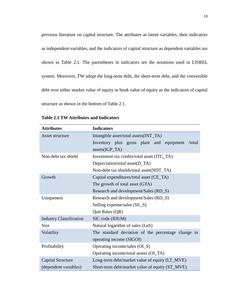
previous literature on capital structure. The attributes as latent variables, their indicators
as independent variables, and the indicators of capital structure as dependent variables are
shown in Table 2.1. The parentheses in indicators are the notations used in LISREL
system. Moreover, TW adopt the long-term debt, the short-term debt, and the convertible
debt over either market value of equity or book value of equity as the indicators of capital
structure as shown in the bottom of Table 2.1.
Table 2.1 TW Attributes and Indicators
Attributes Indicators
Asset structure Intangible asset/total assets(INT_TA)
Inventory plus gross plant and equipment /total
assets(IGP_TA)
Non-debt tax shield
Investment tax credits/total asset (ITC_TA)
Depreciation/total asset(D_TA)
Non-debt tax shields/total asset(NDT_TA)
Growth Capital expenditures/total asset (CE_TA)
The growth of total asset (GTA)
Research and development/Sales (RD_S)
Uniqueness Research and development/Sales (RD_S)
Selling expense/sales (SE_S)
Quit Rates (QR)
Industry Classification SIC code (IDUM)
Size Natural logarithm of sales (LnS)
Volatility The standard deviation of the percentage change in
operating income (SIGOI)
Profitability Operating income/sales (OI_S)
Operating income/total assets (OI_TA)
Capital Structure
(dependent variables)
Long-term debt/market value of equity (LT_MVE)
Short-term debt/market value of equity (ST_MVE)

14
Convertible debt/market value of equity (C_MVE)
Long-term debt/book value of equity (LT_BVE)
Short-term debt/ book value of equity (ST_BVE)
Convertible debt/ book value of equity (C_BVE)
Since we will use confirmatory factor analysis (CFA) approach to test whether
observed variables are good proxies to measure attributes effectively, we add additional
indicators and a financial rating attribute as shown in Table 2.2. These indicators can be
alternative suitable proxies of attributes to replace TW indicators.
Table 2.2 Additional Attributes and Indicators
Attributes Indicators
Growth Research and development/ total assets (RD_TA)
Industry Classification Quit Rates (QR)
Volatility2 Coefficient of Variation of ROA (CV_ROA)
Coefficient of Variation of ROE (CV_ROE)
Coefficient of Variation of Operating Income (CV_OI)
Financial Rating Altman’s Z-score (Z_Score)
S&P Domestic Long Term Issuer Credit Rating
(SP_Rate)
S&P Investment Credit Rating (SP_INV)
Capital Structure
(dependent variables)
Long-term debt/market value of total assets (LT_MVA)
Short-term debt/market value of total assets (ST_MVA)
Convertible debt/market value of total assets (C_MVA)
Long-term debt/book value of total assets (LT_BVA)
Short-term debt/ book value of total assets (ST_BVA)
Convertible debt/ book value of total assets (C_BVA)
2 The additional indicators of volatility are referred to Chang et al. (2008).

15
Asset structure
Based on the trade-off theory and agency theory, firms with larger tangible and
collateral assets may have less bankruptcy, asymmetry information and agency costs.
Myers and Majluf (1984) indicate that companies with larger collateral assets attempt to
issue more secured debt to reduce the cost arising from information asymmetry between
managers and outside investors. Moreover, Jensen and Meckling (1976) and Myers (1977)
state that there are agency costs related to underinvestment problem in the leveraged firm.
High leveraged firm prefer to invest suboptimal investment which only benefits
shareholders and expropriates profits from bondholders. Therefore, the collateral assets
are positive correlated to debt ratios. Rampini and Viswanathan (2013) build a dynamic
agency-based model and claim the importance of collateral asset as a determinant of the
capital structure of a firm.
According to TW paper, the ratio of intangible assets to total assets (INT_TA) and
the ratio of inventory plus gross plant and equipment to total assets (IGP_TA) are viewed
as the indicators to evaluate the asset structure attribute.
Non-debt tax shield
DeAngelo and Masulis (1980) extend Miller’s (1977) model to analyze the effect of
non-debt tax shields increasing the costs of debt for firms. Bowen, Daley, and Huber
16
(1982) find their empirical work on the influence of non-debt tax shields on capital
structure consistent with DeAngelo and Masulis’s (1980) optimal debt model. Graham
(2000) tests how large the effect of tax shield benefits by issuing debts on firms would be
and finds the significant magnitude of tax-reducing value of the interest payments.
However, the firms with large size, more profitability, and high liquidity use less debt as
financing sources even though the reducible tax from interests of debt can profit the
earnings of firms with less bankruptcy possibility. Lin and Flannery (2013) investigate
whether personal taxes affect the cost of debt and equity financing and find that personal
tax is an important determinant of capital structure. Their empirical study shows that tax
cut policy in 2003 has negative influence on firms’ leverage ratio.
Following Fama and French (2000) and TW paper, the indicators of non-debt tax
shields are investment tax credits over total asset (ITC_TA), depreciation over total asset
(D_TA), and non-debt tax shields over total asset (NDT_TA) which NDT is defined as in
TW paper with the corporate tax rate 34%. Since the tax cut policy is a special event, it is
hard to find the indicator of personal tax for all shareholders every year. Therefore, we
left the influence of personal taxes on capital structure for future research.
Growth
According to TW paper, we use capital expenditures over total asset (CE_TA), the
17
growth of total asset (GTA), and research and development over sales (RD_S) as the
indicators of growth attribute. The research and development over total asset (RD_TA)
are added in this attributes to test construct reliability in confirmatory factor analysis3.
TW argue the negative relationship between growth opportunities and debt because
growth opportunities only add firm’s value but cannot collateralize or generate taxable
income.
Uniqueness and Industry Classification
Furthermore, the indicators of uniqueness include development over sales (RD_S)
and selling expense over sales (SE_S). Titman (1984) indicate that uniqueness negatively
correlate to debt because the firms with high level uniqueness will cause customers,
suppliers, and workers to suffer relatively high costs of finding alternative products,
buyers, and jobs when firms liquidate.
SIC code (IDUM) as proxy of industry classification attribute is followed Titman’s
(1984) and TW’s suggestions that firms manufacturing machines and equipment have
high liquidation cost and thus more likely to issue less debt. Graham (2000) uses sales-
and assets- Herfindahl indices to measure industry concentration (Phillips, 1995;
3 Since the denominator of CE_TA and GTA are total asset, RD_TA may reduce the scale problem in
SEM. Therefore, we add RD_TA in growth to test whether the convergent validity of RD_TA is better than
RD_S.

18
Chevalier, 1995) and utilize the dummy of SIC codes to measure product uniqueness.
Graham concluded that more unique of product of a firm, less debt would be used. Here
we assign one to firms in manufacturing industry (SIC codes 3400 to 4000) and zero to
other firms.
Quit Rates (QR) are used in both uniqueness and industry classification to represent
the cost of human capital. Low quit rates implicitly symbolize high level of job-specific
costs that workers encounter costly find alternative jobs in same industry. Therefore, we
expect quit rates negatively related to debt ratio.
Size
The indicator of size attribute is measured by natural logarithm of sales (LnS). The
financing cost of firms may relate to firm size since small firms have higher cost of
non-bank debt financing (see Bevan and Danbolt (2002)). Therefore size is supposed to
be positive associated with debt level.
Volatility and Financial Rating
The previous literature on dynamic capital structural model focused on the trade-off
between the benefits of debt tax shields and the costs of financial distress (Fisher, Heinkel,
and Zechner (1989), Leland and Toft (1996), Leland (1994)).
19
The tax benefits by issuing debts can be offset by the costs of financial distress. Therefore,
Graham (2000) uses Altman’s (1968) Z-score as modified by MacKie-Mason (1990) to
measure bankruptcy and shows that the policy of debt conservatism is positively related
to Z-score. It implies that firms using less of debt can avoid financial distress. Here we
use Altman’s (1986) Z-score4 (Z_Score) as an indicator of financial rating.
Besides, volatility attribute is estimated by the standard deviation of the percentage
change in operating income (SIGOI), Coefficient of Variation of ROA (CV_ROA),
Coefficient of Variation of ROE (CV_ROE), and Coefficient of Variation of Operating
Income (CV_OI). The large variance in earnings means higher possibility of financial
distress; therefore, to avoid bankruptcy happen, firms with larger volatility of earnings
will have less debt.
In addition, we also consider the cost of issuing debt measured by Standard & Poor's
(S&P) Long Term Credit Rating (SP_Rate) and S&P Investment Credit Rating
(SP_INV)5 . High level of financial ratings can decrease the cost of issuing debt.
4 Altman (1968) Z-score formula is:
Z-score = 3.3 ×EBIT
Total Asset+ 0.99 ×
SALE
Total Asset+ 0.6 ×
Market value of Equity
Total Debt+ 1.2 ×
Working Capital
Total Asset+ 1.4 ×
Retained Earnings
Total Asset
5 Standard & Poor's (S&P) Long Term Credit Ratings can be classified into 22 categories on the scale from
AAA to D. Here we give value of these ratings from 1(AAA rating) to 22 (D rating) in order to measure the
attribute of financial ratings. For S&P Investment Credit Rating (SP_INV), we give weights 1 to long-term
investment rating class (AAA to BBB), 2 to non-investment rating class (BB to C), and 3 to default rating
class (SD and D). Thus, firms with higher value (lower level) of S&P long term credit rating will use lower

20
Therefore, according to pecking order theory, the level of financial ratings should be
positively related to the leverage ratio.
Profitability
Finally, the pecking order theory developed in Myers (1977) paper indicates that
firms prefer to use internal finance rather than external finance when raising capital. The
profitable firms are likely to have less debt and profitability in hence is negatively related
to debt level. The pervious empirical studies find the negative relation between debt
usage and profitability which is consistent with the statement of free cash flow problem
by Jensen (1986). However, Stulz (1990) states that a firm would not lose on free cash
flow problem if it has profitable investment opportunities. Graham (2000) uses ROA
(cash flow from operations divided by total assets) as the measure of profitability.
Following TW paper, the indicators of profitability are operating income over sales (OI_S)
and operating income over total assets (OI_TA).
2.2.1.2 Macroeconomic factors
McDonald (1983) extends Miller (1977) theory and investigates the impact of
government financial decisions on capital structure. The equilibrium of McDonald’s
(1983) model shows that the corporate debt-to-wealth ratio is negatively related to the
leverage ratio.

21
government debt-to-wealth ratio. It implies that the decrease in federal borrowing would
lead to the increase in firm’s debt-equity ratio.
The previous studies (Greenwood, Hanson, and Stein, 2010; Bansal, Coleman, and
Lundblad, 2011; Krishnamurthy and Vissing-Jorgensen, 2012; Graham, Leary, and
Roberts, 2012; Greenwood and Vayanos, 2008, 2010) have shown the negative
relationship between government leverage and private sector debt. Bansal, Coleman,
and Lundblad (2011) provide an equilibrium model to illustrate the endogenous supply
relationship between short-term public debt and private debt. They employ Vector
Auto-regression (VAR) to do empirical work and confirm the prediction of their model
that an increase in government leverage leads to the decrease in private debt.
Krishnamurthy and Vissing-Jorgensen (2012) show the negative correlation between the
government leverage and the corporate bond spread which is the difference of yields on
Aaa corporate bonds and long maturity Treasury bonds. When the supply of public debt
decreases, the wide corporate bond spread implies the increase in supply of corporate
debt. This evidence consists with the finding in Greenwood, Hanson, and Stein (2010)
that the issues of private debts seem shifts in supply of government debt. Graham, Leary,
and Roberts (2012) use both macroeconomic factors and firm characteristics to
investigate the determinants of capital structure and find government leverage

22
(debt-to-GDP ratio), which is defined as the ratio of federal debt held by public to GDP,
is an important determinant of variation in aggregate leverage which is defined as the
ratio of aggregate total debt to aggregate book value.
Based on previous literature, we use debt-to-GDP ratio (D_GDP), corporate bond
spread (Spread), and total public debt (TPD) as indicators of macroeconomic attribute to
capital structure. We expect that D_GDP and TPD are negatively related to leverage ratio
and the correlation between leverage ratio and Spread is negative.
2.2.1.3 Manager character
Berger et al. (1997) build a measure of managerial entrenchment to investigate the
agency problem between managers and shareholders, that is, managers would prefer to
issue less debt to benefit their own private profits rather than pursue the optimal capital
structure to benefit shareholders. Berger et al. (1997) find that the usage of debt decrease
with the options and stocks held by CEO, log of number of directors and percentage of
outside directors, but increase with the length of tenure of CEO. Graham (2000) utilize
the same variables from Berger et al. (1997) to measure the managerial entrenchment and
the results are similar to Berger et al. (1997) finding that strong managerial entrenchment
would lead to decrease the debt usage of a firm. The variables used to measure the
managerial entrenchment are the stocks and options held by CEO, the length of working

23
years and tenure of CEO, log of number of directors, percentage of outside directors.
Bhagat, Bolton, and Subramanian (2011) develop a dynamic capital structural model
incorporated with taxes effect, bankruptcy costs and manager characteristics and
investigate the effects of manager characteristics on the firm’s capital structure. Their
model, which incorporates with the concept of agency problems between manager and
shareholders, can be viewed as the application of trade-off theory and agency conflict
problem which utilizes tax effects and bankruptcy costs as external factors and manager
characteristics as internal factors to analysis financing decisions of a firm. Their model
can be viewed as the application of trade-off theory and agency conflict problem which
utilizes tax effects and bankruptcy costs as external factors and manager characteristics as
internal factors to analysis financing decisions of a firm. They find manager
characteristics are important determinants of capital structure decisions and the
manager’s ability is negative correlated to total debt ratio (total debt / total asset) and the
results of their empirical work are consistent with the inference of their model. The
variables, CEO cash compensation, CEO cash compensation to asset ratio, CEO tenure,
CEO tenure divided by CEO age and CEO ownership (numbers of shares of common
stock plus the number of options held by CEO), will be used as the proxies of CEO
ability to test the influence of manager-shareholder agency conflicts on a firm’s financing

24
decisions.
Here we use CEO Tenure over CEO age (Tenu_age), log of CEO tenure (log_Tenu),
log of CEO total compensation (log_TC), CEO bonus (in millions) (Bonus), log of
number of directors (log_Dir) and percentage of outside directors (Out_Dir) as indicators
of manager character. Since both manager’s ability and strong managerial entrenchment
would lead to the decrease of debt usage, the manager character of a firm is expected to
be negatively related to this firm’s leverage.
2.2.2 Joint Determinants of Capital Structure and Stock Rate of Return
Marsh (1982) analyze the empirical study in financing decisions of UK companies
and find their capital structures are heavily influenced by their stock prices. Baker and
Wurgler (2002) provide the empirical evidence that the capital structure of a firm is
significantly related to its historical stock price. The firms prefer to issue equity when
their stock prices are relative high (market-to-book ratio high) and repurchase equity
when the stock prices are relative low. However, the regression equations used in Baker
and Wurgler (2002) seem not very suitable for description of relationship between capital
structure and stock price. The stock price and capital structure change simultaneously
since the stock price will response the investors’ perspective on financing and investment
decisions and managers would take account of both reaction of stock prices and the firm’s
25
long-term equity value when making financing decisions, vice versa. Therefore, we can
use simultaneous structural equation to investigate the relationship between capital
structure and stock price.
Welch (2004) investigates whether companies change their capital structure in
accordance with the changes in stock prices or not. Welch (2004) finds that the stock
price is primary factor of dynamic capital structure. However, the firms don’t readjust
their capital structure to response the changes in stock prices. Jenter (2005) and Jenter et
al. (2011) provide the different aspect of a firm’s financing activity affected by its stock
price. Jenter et al. (2011) state that managers attempt to take advantage of the mispricing
their firms’ equity through corporate financing activities. This behavior is called “time to
market” under the agency problem between the manager and outside investors. The
different beliefs between the manager and investors will cause market timing behavior
(Jung and Subramanian, 2010). Yang (2013) estimate the influence of the difference in
beliefs on firms’ leverage ratio and claim that market timing behavior has the significant
effect on capital structure. The strong investor beliefs (higher stock price) lead to
decreases in firms’ leverage.
Dittmar and Thakor (2007) state a new theory called “managerial investment
autonomy” to explain that a firm’s stock price and its capital structure are simultaneously

26
decided. The “autonomy” means that the firm’s stock price is higher when the likelihood
of investors’ disagreement with investment and financing decisions made from managers
is lower, and vice versa. Since managers consider about the response of shareholders to
the investment decisions and capital financing decisions, managers can use stock prices
as signal whether investors agree or disagree the capital budgeting decisions. Their
empirical findings support the argument that a firm will issue equity rather than debt as
external financing sources when its stock price is high.
For the stock rate of return, we use the annual close prices of a firm in accordance
with its annual reports released date to calculate annual stock returns. Here we add two
attributes, liquidity and value as attributes of stock returns. The indicators of liquidity are
referred from Pastor and Stambaugh’s (2003) innovations in aggregate liquidity
(PS_Innov), level of aggregate liquidity (PS_Level), and traded liquidity factors
(PS_Vwf). The indicators of value are referred to Fama-French five factors6 model:
small minus big (smb), high minus low (hml), excess return on the market (mktrf),
risk-free interest rate used by 1-month T-bill rate (rf), and momentum (umd). In addition,
the attributes of firm characteristics, growth and profitability, are expected to affect stock
6 Fama and French (1992) found three factors related to firm size, excess return on the market, and
book-to-market equity ratio have strong explanation of stock returns.

27
price directly. Therefore, we will set these two attributes as joint determinants of stock
return and capital structure. The list of all indicators and attributes can be found in Table
2.3.
Table 2.3 All Attributes and Indicators
Attributes Indicators
Asset structure
(AtStruct)*
Intangible asset/total assets(INT_TA)
Inventory plus gross plant and equipment /total
assets(IGP_TA)
Non-debt tax shield
(Nd_tax)
Investment tax credits/total asset (ITC_TA)
Depreciation/total asset(D_TA)
Non-debt tax shields/total asset(NDT_TA)
Growth
(Growth)
Capital expenditures/total asset (CE_TA)
The growth of total asset (GTA)
Research and development/Sales (RD_S)
Research and development/ total assets (RD_TA)
Uniqueness
(Unique)
Research and development/Sales (RD_S)
Selling expense/sales (SE_S)
Quit Rates (QR)
Industry classification
(Industry)
SIC code (IDUM)
Quit Rates (QR)
Size (Size) Natural logarithm of sales (LnS)
Volatility
(Vol)
The standard deviation of the percentage change in
operating income (SIGOI)
Coefficient of Variation of ROA (CV_ROA)
Coefficient of Variation of ROE (CV_ROE)
Coefficient of Variation of Operating Income (CV_OI)
Profitability
(Profit)
Operating income/sales (OI_S)
Operating income/total assets (OI_TA)
Financial rating
(Rate)
Altman’s Z-score (Z_Score)
S&P Domestic Long Term Issuer Credit Rating
(SP_Rate)
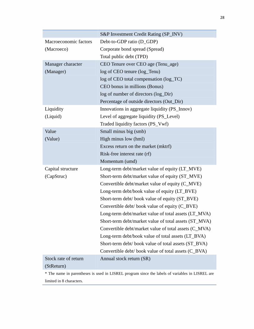
28
S&P Investment Credit Rating (SP_INV)
Macroeconomic factors
(Macroeco)
Debt-to-GDP ratio (D_GDP)
Corporate bond spread (Spread)
Total public debt (TPD)
Manager character
(Manager)
CEO Tenure over CEO age (Tenu_age)
log of CEO tenure (log_Tenu)
log of CEO total compensation (log_TC)
CEO bonus in millions (Bonus)
log of number of directors (log_Dir)
Percentage of outside directors (Out_Dir)
Liquidity
(Liquid)
Innovations in aggregate liquidity (PS_Innov)
Level of aggregate liquidity (PS_Level)
Traded liquidity factors (PS_Vwf)
Value
(Value)
Small minus big (smb)
High minus low (hml)
Excess return on the market (mktrf)
Risk-free interest rate (rf)
Momentum (umd)
Capital structure
(CapStruc)
Long-term debt/market value of equity (LT_MVE)
Short-term debt/market value of equity (ST_MVE)
Convertible debt/market value of equity (C_MVE)
Long-term debt/book value of equity (LT_BVE)
Short-term debt/ book value of equity (ST_BVE)
Convertible debt/ book value of equity (C_BVE)
Long-term debt/market value of total assets (LT_MVA)
Short-term debt/market value of total assets (ST_MVA)
Convertible debt/market value of total assets (C_MVA)
Long-term debt/book value of total assets (LT_BVA)
Short-term debt/ book value of total assets (ST_BVA)
Convertible debt/ book value of total assets (C_BVA)
Stock rate of return
(StReturn)
Annual stock return (SR)
* The name in parentheses is used in LISREL program since the labels of variables in LISREL are
limited in 8 characters.
29
2.2.3 Data
Since the data for indicators of firm characteristics, macroeconomic factors,
manager character, and the determinants of stock returns are collected from different
datasets, the sample period is constrained by the common period of these datasets. The
sample period is 2001 to 2012. The annual stock price and data of firm characteristics
except quit rates are collected from Compustat. S&P Credit Rating information can be
obtained in rating category of Compustat. The time length to measure the indicators of
volatility attribute is 5 years (past four years to current year).The codes of the accounting
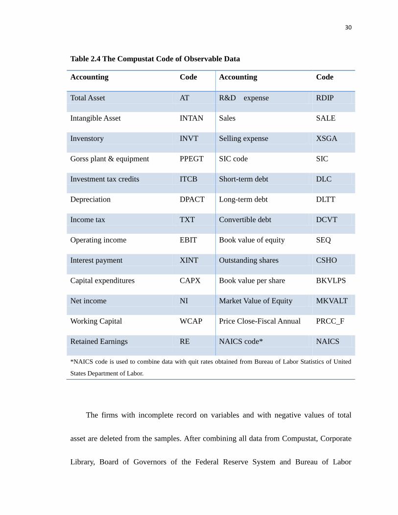
items used to calculate the observed variables in Compustat are shown in Table 2.4.
The data used for manager character, macroeconomic factors, and quit rates are
collected from Corporate Library, Board of Governors of the Federal Reserve System and
Bureau of Labor Statistics of United States Department of Labor, respectively. The Pastor
and Stambaugh’s (2003) three liquidity7 factors and Fama-French five factors are
collected from Fama-French Portfolios and Factors dataset in WRDS. Since the data from
Fama-French Portfolios and Factors dataset is monthly data, we combine them with other
data by calendar date. Because these factors are used to forecast stock returns, the
measuring year of these factors is one month before annual report released date.
7 The details of liquidity factors are described in Pastor and Stambaugh (2003).
30
Table 2.4 The Compustat Code of Observable Data
Accounting Code Accounting Code
Total Asset AT R&D expense RDIP
Intangible Asset INTAN Sales SALE
Invenstory INVT Selling expense XSGA
Gorss plant & equipment PPEGT SIC code SIC
Investment tax credits ITCB Short-term debt DLC
Depreciation DPACT Long-term debt DLTT
Income tax TXT Convertible debt DCVT
Operating income EBIT Book value of equity SEQ
Interest payment XINT Outstanding shares CSHO
Capital expenditures CAPX Book value per share BKVLPS
Net income NI Market Value of Equity MKVALT
Working Capital WCAP Price Close-Fiscal Annual PRCC_F
Retained Earnings RE NAICS code* NAICS
*NAICS code is used to combine data with quit rates obtained from Bureau of Labor Statistics of United
States Department of Labor.
The firms with incomplete record on variables and with negative values of total
asset are deleted from the samples. After combining all data from Compustat, Corporate
Library, Board of Governors of the Federal Reserve System and Bureau of Labor

31
Statistics of United States Department of Labor, total sample size during 2001 to 2012 is
3118.
2.3 Methodologies and LISREL System
In this section, we first introduce the SEM approach and present an example of path
diagram to show the structure of structural model and measurement model in SEM
framework. Subsequently, Multiple Indicators Multiple Causes (MIMIC) model and its
path diagram show alternative way to investigate the determinants of capital structure.
Finally, Confirmatory Factor Analysis (CFA) is provided to improve the explanation of
relations between indicators and latent variables in measurement model of SEM
framework.
2.3.1 SEM Approach
The SEM incorporates three equations as follows:
𝑆𝑡𝑟𝑢𝑐𝑡𝑢𝑟𝑎𝑙 𝑚𝑜𝑑𝑒𝑙: 𝜂 = 𝛽𝜂 + Φ𝜉 + 𝜍 (2.1)
𝑀𝑒𝑎𝑠𝑢𝑟𝑒𝑚𝑒𝑛𝑡 𝑚𝑜𝑑𝑒𝑙 𝑓𝑜𝑟 𝑦: 𝑦 = Λy𝜂 + 𝜐 (2.2)
𝑀𝑒𝑎𝑠𝑢𝑟𝑒𝑚𝑒𝑛𝑡 𝑚𝑜𝑑𝑒𝑙 𝑓𝑜𝑟 𝑥: 𝑥 = Λ𝜉 + 𝛿 (2.3)
x is the matrix of observed independent variables as the indicators of attributes, y is the
matrix of observed dependent variables as the indicators of capital structure, 𝜉 is the
32
matrix of latent variables as attributes, 𝜂 is the latent variables that link determinants of
capital structure (a linear function of attributes) to capital structure(y).
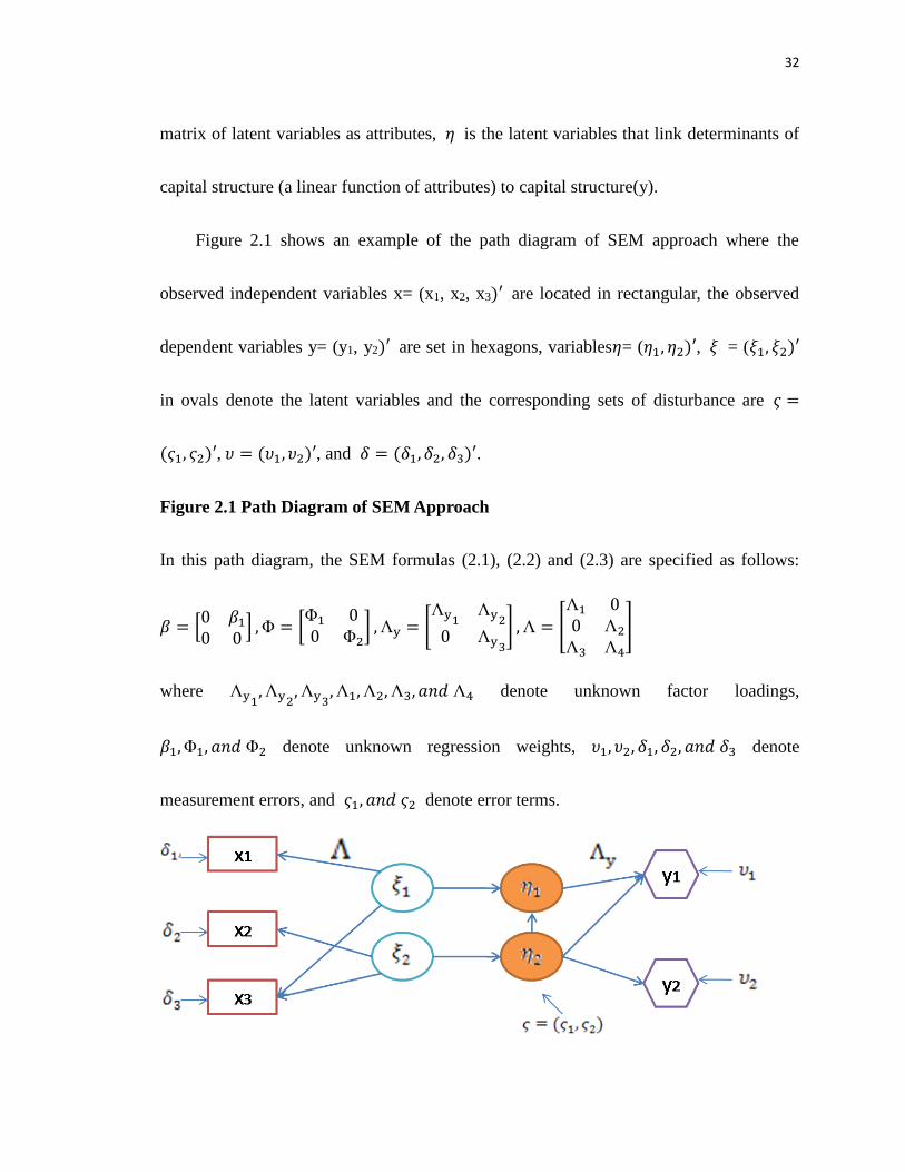
Figure 2.1 shows an example of the path diagram of SEM approach where the
observed independent variables x= (x1, x2, x3)′ are located in rectangular, the observed
dependent variables y= (y1, y2)′ are set in hexagons, variables𝜂= (𝜂1, 𝜂2)′, 𝜉 = (𝜉1, 𝜉2)′
in ovals denote the latent variables and the corresponding sets of disturbance are 𝜍 =
(𝜍1, 𝜍2)′, 𝜐 = (𝜐1, 𝜐2)′, and 𝛿 = (𝛿1, 𝛿2, 𝛿3)′.
Figure 2.1 Path Diagram of SEM Approach
In this path diagram, the SEM formulas (2.1), (2.2) and (2.3) are specified as follows:
𝛽 = [0 𝛽10 0
] ,Φ = [Φ1 00 Φ2
] ,Λy = [Λy1
Λy2
0 Λy3
] ,Λ = [
Λ1 00 Λ2
Λ3 Λ4
]
where Λy1,Λy2
,Λy3,Λ1,Λ2,Λ3, 𝑎𝑛𝑑 Λ4 denote unknown factor loadings,
𝛽1,Φ1, 𝑎𝑛𝑑 Φ2 denote unknown regression weights, 𝜐1, 𝜐2, 𝛿1, 𝛿2, 𝑎𝑛𝑑 𝛿3 denote
measurement errors, and 𝜍1, 𝑎𝑛𝑑 𝜍2 denote error terms.

33
The structural model can be specified as the system of equations which combines
equations (2.1) and (2.2), and then we can obtain the structural model in TW paper as
follows:
𝑦 = Γ𝜉 + 휀 (2.4)
In this paper, the accounting items can be viewed as the observable independent
variables (x) which are the causes of attributes as the latent variables (𝜉) ,and the
debt-equity ratios represented the indicators of capital structure are the observable
dependent variables (y).
The fitting function for maximum likelihood estimation method for SEM approach
is:
𝐹 = 𝑙𝑜𝑔|Σ| + 𝑡𝑟(𝑆Σ−1) − 𝑙𝑜𝑔|𝑆| − (𝑝 + 𝑞) (2.5)
where S is the observed covariance matrix, Σ is the model-implied covariance matrix, p
is the number of independent variables (x), and q is the number of dependent variables
(y).
2.3.2 Illustration of SEM Approach in LISREL System
In general, SEM consists of two parts, the measurement model and structural model. The
measurement model analysis the presumed relations between the latent variables viewed

34
as the attributes and observable variables viewed as the indicators. For example, capital
expenditures over total assets (CE_TA) and research and development over sales (RD_S)
are the indicators of the growth attributes (Growth). In the measurement model, each
indicator is assumed to have measurement error associated with it. On the other hand, the
structure model presents the relationship between unobserved variables and outcome. For
instance, the relationship between attributes and the capital structure is represented by the
structure model. The relationship between the capital structure and its indicators
estimated by debt-equity ratios and debt-asset ratios is modeled by the measurement
model.
35
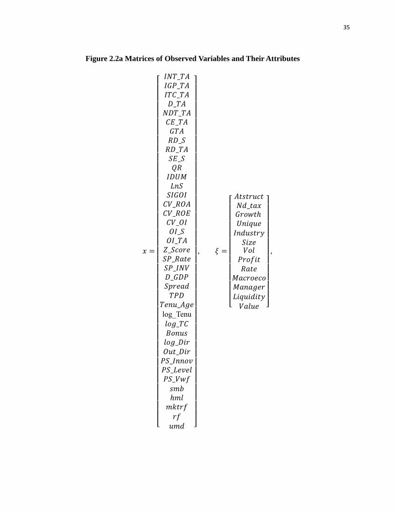
Figure 2.2a Matrices of Observed Variables and Their Attributes
𝑥 =
[ 𝐼𝑁𝑇_𝑇𝐴𝐼𝐺𝑃_𝑇𝐴𝐼𝑇𝐶_𝑇𝐴𝐷_𝑇𝐴𝑁𝐷𝑇_𝑇𝐴𝐶𝐸_𝑇𝐴𝐺𝑇𝐴𝑅𝐷_𝑆𝑅𝐷_𝑇𝐴𝑆𝐸_𝑆𝑄𝑅𝐼𝐷𝑈𝑀𝐿𝑛𝑆𝑆𝐼𝐺𝑂𝐼𝐶𝑉_𝑅𝑂𝐴𝐶𝑉_𝑅𝑂𝐸𝐶𝑉_𝑂𝐼𝑂𝐼_𝑆𝑂𝐼_𝑇𝐴𝑍_𝑆𝑐𝑜𝑟𝑒𝑆𝑃_𝑅𝑎𝑡𝑒𝑆𝑃_𝐼𝑁𝑉𝐷_𝐺𝐷𝑃𝑆𝑝𝑟𝑒𝑎𝑑𝑇𝑃𝐷
𝑇𝑒𝑛𝑢_𝐴𝑔𝑒log_Tenu
𝑙𝑜𝑔_𝑇𝐶 𝐵𝑜𝑛𝑢𝑠𝑙𝑜𝑔_𝐷𝑖𝑟 𝑂𝑢𝑡_𝐷𝑖𝑟𝑃𝑆_𝐼𝑛𝑛𝑜𝑣𝑃𝑆_𝐿𝑒𝑣𝑒𝑙𝑃𝑆_𝑉𝑤𝑓𝑠𝑚𝑏ℎ𝑚𝑙𝑚𝑘𝑡𝑟𝑓𝑟𝑓𝑢𝑚𝑑 ]
, 𝜉 =
[ 𝐴𝑡𝑠𝑡𝑟𝑢𝑐𝑡𝑁𝑑_𝑡𝑎𝑥𝐺𝑟𝑜𝑤𝑡ℎ 𝑈𝑛𝑖𝑞𝑢𝑒𝐼𝑛𝑑𝑢𝑠𝑡𝑟𝑦𝑆𝑖𝑧𝑒𝑉𝑜𝑙
𝑃𝑟𝑜𝑓𝑖𝑡𝑅𝑎𝑡𝑒
𝑀𝑎𝑐𝑟𝑜𝑒𝑐𝑜𝑀𝑎𝑛𝑎𝑔𝑒𝑟𝐿𝑖𝑞𝑢𝑖𝑑𝑖𝑡𝑦𝑉𝑎𝑙𝑢𝑒 ]
,
36
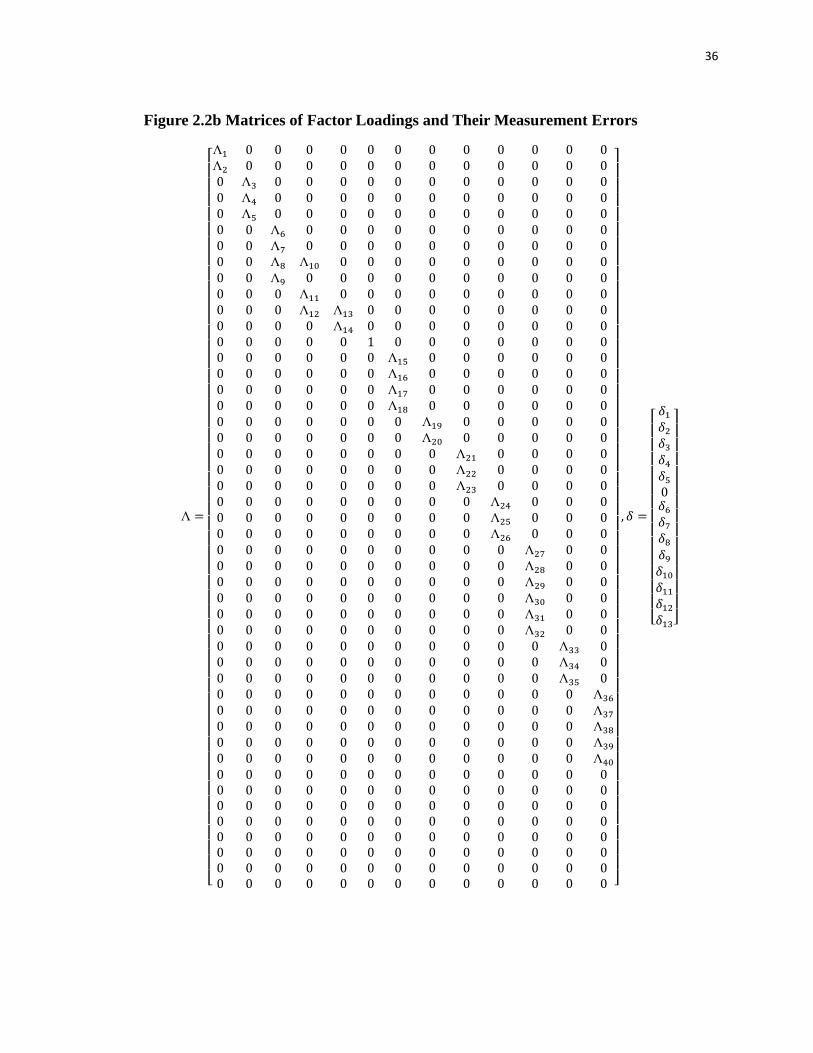
Figure 2.2b Matrices of Factor Loadings and Their Measurement Errors
Λ =
[ Λ1 0 0 0 0 0 0 0 0 0 0 0 0Λ2 0 0 0 0 0 0 0 0 0 0 0 00 Λ3 0 0 0 0 0 0 0 0 0 0 00 Λ4 0 0 0 0 0 0 0 0 0 0 00 Λ5 0 0 0 0 0 0 0 0 0 0 00 0 Λ6 0 0 0 0 0 0 0 0 0 00 0 Λ7 0 0 0 0 0 0 0 0 0 00 0 Λ8 Λ10 0 0 0 0 0 0 0 0 00 0 Λ9 0 0 0 0 0 0 0 0 0 00 0 0 Λ11 0 0 0 0 0 0 0 0 00 0 0 Λ12 Λ13 0 0 0 0 0 0 0 00 0 0 0 Λ14 0 0 0 0 0 0 0 00 0 0 0 0 1 0 0 0 0 0 0 00 0 0 0 0 0 Λ15 0 0 0 0 0 00 0 0 0 0 0 Λ16 0 0 0 0 0 00 0 0 0 0 0 Λ17 0 0 0 0 0 00 0 0 0 0 0 Λ18 0 0 0 0 0 00 0 0 0 0 0 0 Λ19 0 0 0 0 00 0 0 0 0 0 0 Λ20 0 0 0 0 00 0 0 0 0 0 0 0 Λ21 0 0 0 00 0 0 0 0 0 0 0 Λ22 0 0 0 00 0 0 0 0 0 0 0 Λ23 0 0 0 00 0 0 0 0 0 0 0 0 Λ24 0 0 00 0 0 0 0 0 0 0 0 Λ25 0 0 00 0 0 0 0 0 0 0 0 Λ26 0 0 00 0 0 0 0 0 0 0 0 0 Λ27 0 00 0 0 0 0 0 0 0 0 0 Λ28 0 00 0 0 0 0 0 0 0 0 0 Λ29 0 00 0 0 0 0 0 0 0 0 0 Λ30 0 00 0 0 0 0 0 0 0 0 0 Λ31 0 00 0 0 0 0 0 0 0 0 0 Λ32 0 00 0 0 0 0 0 0 0 0 0 0 Λ33 00 0 0 0 0 0 0 0 0 0 0 Λ34 00 0 0 0 0 0 0 0 0 0 0 Λ35 00 0 0 0 0 0 0 0 0 0 0 0 Λ36
0 0 0 0 0 0 0 0 0 0 0 0 Λ37
0 0 0 0 0 0 0 0 0 0 0 0 Λ38
0 0 0 0 0 0 0 0 0 0 0 0 Λ39
0 0 0 0 0 0 0 0 0 0 0 0 Λ40
0 0 0 0 0 0 0 0 0 0 0 0 00 0 0 0 0 0 0 0 0 0 0 0 00 0 0 0 0 0 0 0 0 0 0 0 00 0 0 0 0 0 0 0 0 0 0 0 00 0 0 0 0 0 0 0 0 0 0 0 00 0 0 0 0 0 0 0 0 0 0 0 00 0 0 0 0 0 0 0 0 0 0 0 00 0 0 0 0 0 0 0 0 0 0 0 0 ]
, 𝛿 =
[ 𝛿1𝛿2𝛿3𝛿4𝛿50𝛿6𝛿7𝛿8𝛿9𝛿10𝛿11𝛿12𝛿13]
37
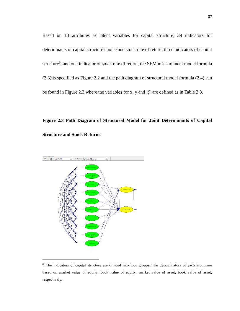
Based on 13 attributes as latent variables for capital structure, 39 indicators for
determinants of capital structure choice and stock rate of return, three indicators of capital
structure8, and one indicator of stock rate of return, the SEM measurement model formula
(2.3) is specified as Figure 2.2 and the path diagram of structural model formula (2.4) can
be found in Figure 2.3 where the variables for x, y and 𝜉 are defined as in Table 2.3.
Figure 2.3 Path Diagram of Structural Model for Joint Determinants of Capital
Structure and Stock Returns
8 The indicators of capital structure are divided into four groups. The denominators of each group are
based on market value of equity, book value of equity, market value of asset, book value of asset,
respectively.

38
2.3.3 Multiple Indicators Multiple Causes (MIMIC) Model
MIMIC model is the specified SEM that uses latent variables to investigate the
relationship between the indicators and causes of these latent variables. The MIMIC
model incorporates two equations as follows:
𝜂 = 𝛾𝑥 + 𝜍 (2.5)
𝑦 = λ𝜂 + 𝜐 (2.6)
𝜂 is the matrix of latent variables that link determinants of capital structure(x) to capital
structure(y); x is the matrix of observed independent variables as the causes of 𝜂; y is the
matrix of observed dependent variables as the indicators of 𝜂; 𝜍 and 𝜐 are error terms.
In this essay, there is only one latent variable in 𝜂, which is called leverage.
Figure 2.4 shows an example of the path diagram of MIMIC model where the
observed independent variables x= (x1, x2, x3)′ are located in rectangular, the observed
dependent variables y= (y1, y2)′ are set in hexagons, variables 𝜂= (𝜂1, 𝜂2)′, in ovals
denote the latent variables and the corresponding sets of disturbance are 𝜍 = (𝜍1, 𝜍2)′,
and 𝜐 = (𝜐1, 𝜐2)′.
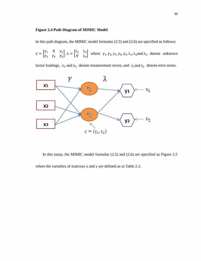
39
Figure 2.4 Path Diagram of MIMIC Model
In this path diagram, the MIMIC model formulas (2.5) and (2.6) are specified as follows:
𝛾 = [𝛾1 0 𝛾2𝛾3 𝛾4 𝛾5
] , λ = [λ1 λ20 λ3
] where 𝛾1, 𝛾2, 𝛾3, 𝛾4, 𝛾5, λ1, λ2and λ3 denote unknown
factor loadings, 𝜐1 and 𝜐2 denote measurement errors, and 𝜍1and 𝜍2 denote error terms.
In this essay, the MIMIC model formulas (2.5) and (2.6) are specified as Figure 2.5
where the variables of matrixes x and y are defined as in Table 2.3.

40
Figure 2.5 Matrices for Determinants of Capital Structure and Stock Rate of Return
in MIMIC model
𝑥 =
[ 𝐼𝑁𝑇_𝑇𝐴𝐼𝐺𝑃_𝑇𝐴𝐼𝑇𝐶_𝑇𝐴𝐷_𝑇𝐴𝑁𝐷𝑇_𝑇𝐴𝐶𝐸_𝑇𝐴𝐺𝑇𝐴𝑅𝐷_𝑆𝑅𝐷_𝑇𝐴𝑆𝐸_𝑆𝑄𝑅𝐼𝐷𝑈𝑀𝐿𝑛𝑆𝑆𝐼𝐺𝑂𝐼𝐶𝑉_𝑅𝑂𝐴𝐶𝑉_𝑅𝑂𝐸𝐶𝑉_𝑂𝐼𝑂𝐼_𝑆𝑂𝐼_𝑇𝐴𝑍_𝑆𝑐𝑜𝑟𝑒𝑆𝑃_𝑅𝑎𝑡𝑒𝑆𝑃_𝐼𝑁𝑉𝐷_𝐺𝐷𝑃𝑆𝑝𝑟𝑒𝑎𝑑𝑇𝑃𝐷
𝑇𝑒𝑛𝑢_𝐴𝑔𝑒log_Tenu
log_TC𝐵𝑜𝑛𝑢𝑠 log_Dir𝑂𝑢𝑡_𝐷𝑖𝑟𝑃𝑆_𝐼𝑛𝑛𝑜𝑣𝑃𝑆_𝐿𝑒𝑣𝑒𝑙𝑃𝑆_𝑉𝑤𝑓𝑠𝑚𝑏ℎ𝑚𝑙𝑚𝑘𝑡𝑟𝑓𝑟𝑓𝑢𝑚𝑑 ]
, 𝜂 = [𝐶𝑎𝑝𝑆𝑡𝑟𝑢𝑐𝑆𝑡𝑅𝑒𝑡𝑢𝑟𝑛
] , 𝑦 = [
𝐿𝑇_𝑀𝑉𝐴𝑆𝑇_𝑀𝑉𝐴𝐶_𝑀𝑉𝐴𝑆𝑅
] , λ = [
λ1 0λ2 0λ3 00 1
] , 𝜐 = [
𝜐1 0𝜐2 0𝜐3 00 0
]
𝛾 = [𝛾1 ⋯⋯⋯⋯⋯⋯⋯⋯⋯⋯⋯⋯⋯⋯⋯⋯⋯⋯⋯⋯⋯⋯ 𝛾390⋯0 𝛾6𝛾7𝛾8𝛾9 0⋯0 𝛾18𝛾19 0⋯ 0 𝛾32 𝛾33𝛾34𝛾35 𝛾36𝛾37𝛾38 𝛾39
] , 𝜍 = [𝜍1, 𝜍2]
41
2.3.4 Confirmatory Factor Analysis (CFA)
In SEM framework, the usage of confirmatory factor analysis (CFA) in
measurement model is to test whether the data fit a hypothesized measurement model
which is based on theories in previous literature. CFA is usually utilized as the first step
to assess a designed measurement model in SEM since it is a theory-driven analysis that
evaluates the consistency between a priori hypotheses and the parameter estimates in the
relations between observed variables and latent variables. If CFA shows the poor
confirmation of a measurement model, and then the results of SEM will indicate a poor
fit, the model will be rejected, and the parameter estimates will be unexplainable.
Therefore, we should first utilize CFA to adjust the relations between observed and latent
variables in SEM, and subsequently conclude the results in accordance with assessment
of model fit statistics9.
CFA can evaluate the confirmation of a designed model via the construct validity of
a proposed measurement theory. Two major validities, convergent validity and
discriminant validity, are the important components of construct validity which is the
extent to test whether a set of measured items actually reflects the theoretical latent
9 With regard to selecting model-fit evaluation, CFI (Comparative-Fit Index), RMSEA (Root Mean Square
Error of Approximation), the ratio of Chi-Square value to degree of freedom, and SRMR (Standardized
Root Mean Square Residual) are common goodness-of-fit measures.

42
construct in measurement model. There are three approaches to evaluate convergent
validity: factor loadings, average variance extracted (AVE), and composite reliability
(CR). In general, the factor loadings (the parameter estimates) larger than the critical
value 0.5 imply that the latent variables can appropriately explain the observed variables
and the measurement model has good convergent validity. The formulas of average
variance extracted (AVE) and composite reliability (CR) for a latent variable are as
follows:
𝐴𝑉𝐸 =∑𝜆2
∑𝜆2 + ∑𝜃
𝐶𝑅 =(∑𝜆)2
(∑ 𝜆)2 + ∑𝜃
Where 𝜆 denotes the standardized factor loadings (the standardized parameter
estimates) of a latent variable and 𝜃 denotes the indicator error variances of observed
variables related to this latent variable. In LISREL system, we can obtain Squared
Multiple Correlations (SMC) of observed variables. SMC value can be viewed as the
coefficient of determination, R2 in linear regression analysis, and the value 𝜃 of an
observed variable equals to the value of one minus SMC of that observed variable. If
AVE and CR of a latent variable are larger than 0.5, then this latent variable is reasonably
set in measurement model and the model has good convergent validity of this latent
variable.

43
In addition, there are three ways to measure discriminant validity of a measurement
model. The first method is to compare the original measurement model with the restricted
measurement model which fixes the coefficient of correlation between two latent
variables equal to 1.00. Secondly, the alternative method of setting the restricted
measurement model is to combine two latent variables into one latent variable in the
model. If the difference of Chi-Square value of the original and the restricted models is
significant10, then the set of measurement model performs good discriminant validity and
the latent variables are of significant difference that can represent different characteristics
in SEM. The third method is the comparison of AVE value of a latent variable and the
square of the coefficient of correlation between two latent variables; if the square of the
coefficient of correlation between two latent variables is larger than both AVE of these
latent variables, then these latent variables can perform discriminative characters well.
2.4 Empirical Analysis
In this section, we first do empirical work on determinants of capital structure and
then investigate the joint determinants of capital structure and stock rate of return. We use
both SEM with CFA and MIMIC model to illustrate the structural equal modeling
10 The 5% and 1% significant value of the difference of Chi-Square value between original measurement
model and the restricted model are 3.841 and 6.64 respectively.

44
approach and compare their results. Finally, we will compare our results to the empirical
results of TW, Chang et al. (2008) and Yang et al. (2010).
2.4.1 Determinants of Capital Structure by SEM with CFA
During CFA test, we delete some indicators to solve singularity problem in
covariance matrix and combines some attributes to satisfy discriminant and convergent
validity measures11. The conceptual diagram of structure model for determinants of
capital structure is illustrated in Figure 2.6. Here we combine attributes, uniqueness and
industry classification, into one attribute called “Uni_Ind” to solve the collinearity
problem since the indicators of these attributes are similar. Another combined attribute is
called “Vol_Rate” from volatility and financial rating attributes because both attributes
are used to measure financial distress costs.
The estimates of the parameters of measurement model without CFA are presented in
Table2.5 and Table 2.7. There are 23 indicators and 9 attributes in SEM with CFA model
for determinants of capital structure12.
11 The Chi-Square value = 6905.61, Degree of Freedom = 252, Normed Fit Index (NFI) = 0.79,
Comparative Fit Index (CFI) = 0.79, Root Mean Square Error of Approximation (RMSEA) = 0.092, Root
Mean Square Residual (RMR) = 0.15, Standardized RMR = 0.076 and Goodness of Fit Index (GFI) = 0.85.
Since the sample size is too big, the insignificant value of Chi-Square cannot be good indicator of model
fitness. Based on CFA criteria, CFI, GFI, RMSEA and RMR show our model is acceptable.
12 We have collected 31 indicators to analyze the determinants of capital structure. However, the
covariance matrix is not positive definite and results in singularity problem. Therefore, we delete some
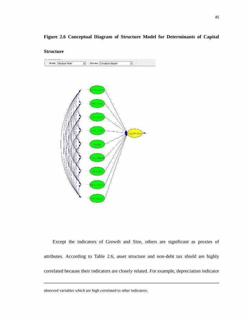
45
Figure 2.6 Conceptual Diagram of Structure Model for Determinants of Capital
Structure
Except the indicators of Growth and Size, others are significant as proxies of
attributes. According to Table 2.6, asset structure and non-debt tax shield are highly
correlated because their indicators are closely related. For example, depreciation indicator
observed variables which are high correlated to other indicators.

46
(D_TA) of non-debt tax shield is positively related to gross plant and equipment indicator
(IGP_TA) of asset structure. The high correlation of attributes will cause problems in
estimating the model. In addition, too many latent variables and the lack of using
indicators with unique weights corresponding to their attributes may also cause the week
results (Maddala and Nimalendran, 1996). Therefore, we can expect more significant
results if we delete either asset structure or non-debt tax shield attribute. We will also
remove some insignificant attributes, e.g. growth or size, to test whether the results are
more significant under confirmatory factor analysis.
Based on the results in Table 2.7, we find profitability having significant effect on
capital structure in either short-term or long-term aspect. The positive relationship
between profitability and capital structure is inconsistent with pecking order theory
(Myers, 1977) and free cash flow theory (Jensen, 1986). However, we can infer that
profitable firms may utilize both internal sources and debts to invest profitable
opportunities and to avoid agency costs (Stulz, 1990). Volatility and financial rating only
influence on market-based short-term leverage ratio. This evidence implies that even
though the credit risk affects the fluctuation of stock price, bankruptcy cost may not
change long-term target leverage ratios. It also consists with Welch’s (2004) inference
that firms don’t readjust target leverage ratios responding to their fluctuated stock prices.
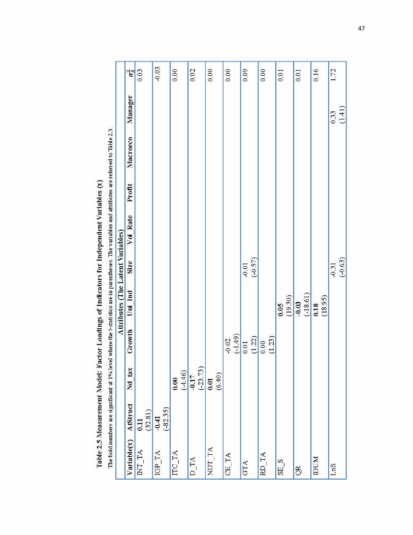
47
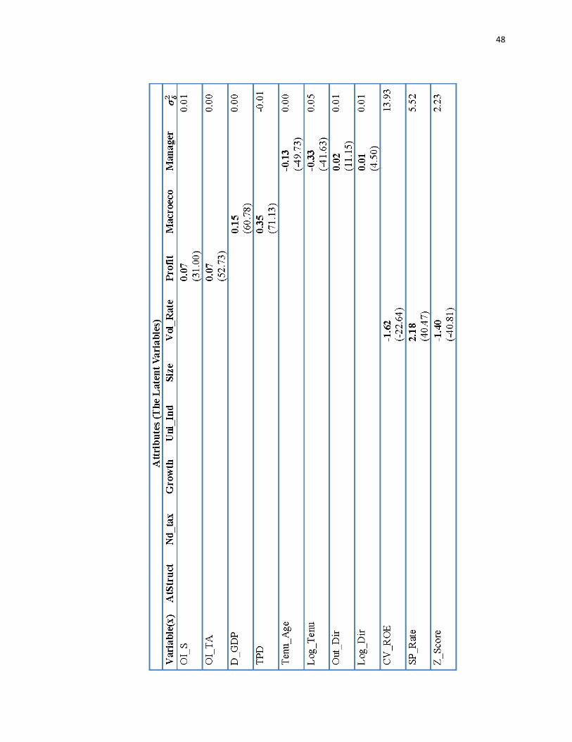
48
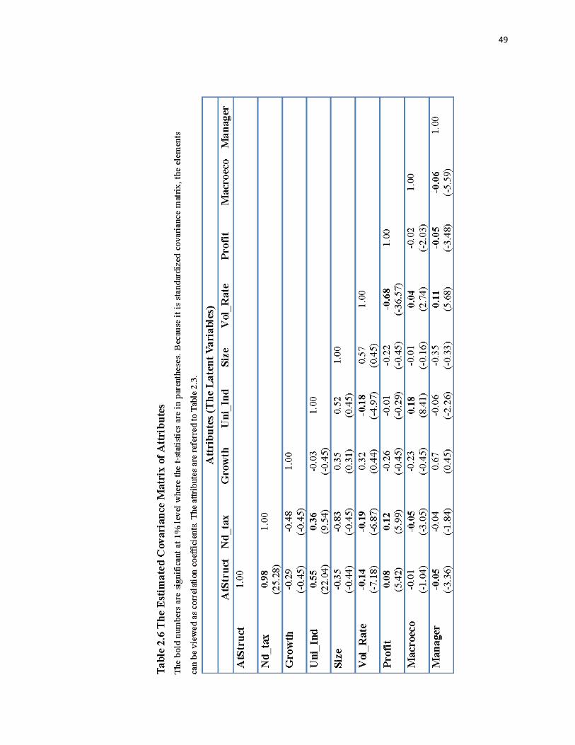
49
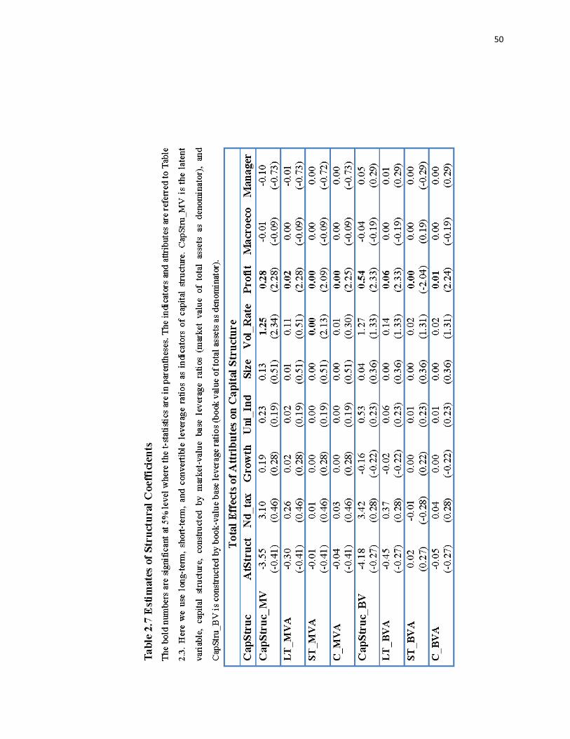
50

51
2.4.2 Determinants of Capital Structure by MIMIC Model
To enhance the explanation of the factors of capital structure, I use MIMIC model to
reduce the latent variable and improve the results shown in Figure 2.7 and Table 2.8. The
standardized estimates of determinants of capital structure in market value basis are
illustrated by path diagram in Figure 2.7 where there is only one latent variable (attribute),
Capital Structure (CapStruc), and all observed variables are the indicators of this attribute.
The selection of indicators for determinants of capital structure in MIMIC model is same
as it in SEM with CFA to compare the performance between two models. The
goodness-of-fit measures show that MIMIC model performed better than SEM with
CFA13 because of the decrease in latent variables.
The parameter estimates of determinants of capital structure in both market value
basis and book value basis are shown in Table 2.8. Compared to SEM with CFA method,
at least one indicator of attributes, AtStruct, Nd_tax, Growth, Uni_Ind, Vol_Rate and
Macroeco, has explanation power of capital structure in both market and book value
13 The Chi-Square value = 678.80, Degree of Freedom = 46, Normed Fit Index (NFI) = 0.98, Comparative
Fit Index (CFI) = 0.98, Root Mean Square Error of Approximation (RMSEA) = 0.066, Root Mean Square
Residual (RMR) = 0.0013, Standardized RMR = 0.029 and Goodness of Fit Index (GFI) = 0.98. Since the
sample size is too big, the insignificant value of Chi-Square cannot be good indicator of model fitness.
Based on CFA criteria, CFI, GFI, RMSEA and RMR show our model is acceptable. The goodness-of-fit
measure, RMR and RMSEA in MIMIC model smaller the values in SEM with CFA shows MIMIC model
performed better than SEM with CFA.

52
bases. Size and Profit attributes only have significant effects on leverage ratios in book
value basis. In addition, manager only influences on capital structure in market value
basis.
Although there are many significant indicators to determine capital structure, some
of them are incompatible with each others. For example, INT_TA and IGP_TA should
have inversely influences on capital structure while they both are positively related to
capital structure in MIMIC model. All indicators of Nd_tax should be negatively relation
to capital structure while NDT_TA has significantly positive relation to it. Therefore, we
would claim that SEM with CFA would be more proper to investigate the determinants of
capital structure rather than MIMIC model if we can establish SEM with CFA under
better goodness-of-fit measures.
According to the results in both SEM with CFA and MIMIC model, the long-term
debt ratio in both market and book value bases has heavy factor loading in capital
structure. Therefore, we claim that the factors of capital structure focus on long-term
rather than short-term leverage ratios.
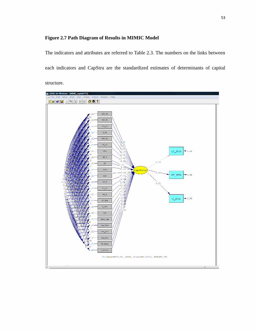
53
Figure 2.7 Path Diagram of Results in MIMIC Model
The indicators and attributes are referred to Table 2.3. The numbers on the links between
each indicators and CapStru are the standardized estimates of determinants of capital
structure.
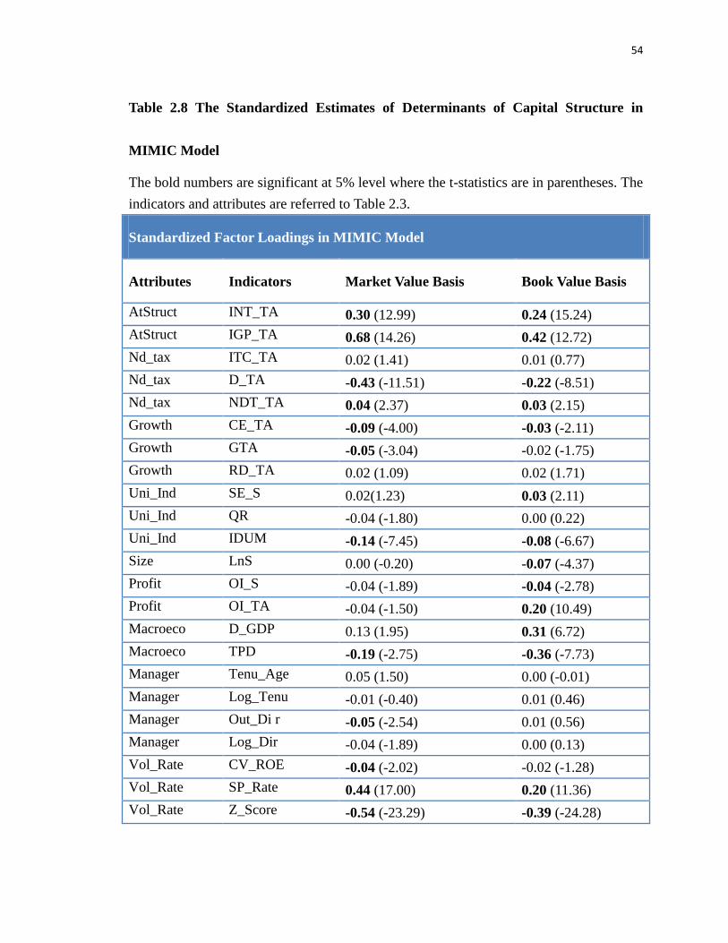
54
Table 2.8 The Standardized Estimates of Determinants of Capital Structure in
MIMIC Model
The bold numbers are significant at 5% level where the t-statistics are in parentheses. The
indicators and attributes are referred to Table 2.3.
Standardized Factor Loadings in MIMIC Model
Attributes Indicators Market Value Basis Book Value Basis
AtStruct INT_TA 0.30 (12.99) 0.24 (15.24)
AtStruct IGP_TA 0.68 (14.26) 0.42 (12.72)
Nd_tax ITC_TA 0.02 (1.41) 0.01 (0.77)
Nd_tax D_TA -0.43 (-11.51) -0.22 (-8.51)
Nd_tax NDT_TA 0.04 (2.37) 0.03 (2.15)
Growth CE_TA -0.09 (-4.00) -0.03 (-2.11)
Growth GTA -0.05 (-3.04) -0.02 (-1.75)
Growth RD_TA 0.02 (1.09) 0.02 (1.71)
Uni_Ind SE_S 0.02(1.23) 0.03 (2.11)
Uni_Ind QR -0.04 (-1.80) 0.00 (0.22)
Uni_Ind IDUM -0.14 (-7.45) -0.08 (-6.67)
Size LnS 0.00 (-0.20) -0.07 (-4.37)
Profit OI_S -0.04 (-1.89) -0.04 (-2.78)
Profit OI_TA -0.04 (-1.50) 0.20 (10.49)
Macroeco D_GDP 0.13 (1.95) 0.31 (6.72)
Macroeco TPD -0.19 (-2.75) -0.36 (-7.73)
Manager Tenu_Age 0.05 (1.50) 0.00 (-0.01)
Manager Log_Tenu -0.01 (-0.40) 0.01 (0.46)
Manager Out_Di r -0.05 (-2.54) 0.01 (0.56)
Manager Log_Dir -0.04 (-1.89) 0.00 (0.13)
Vol_Rate CV_ROE -0.04 (-2.02) -0.02 (-1.28)
Vol_Rate SP_Rate 0.44 (17.00) 0.20 (11.36)
Vol_Rate Z_Score -0.54 (-23.29) -0.39 (-24.28)

55
2.4.3 Joint Determinants of Capital Structure and Stock Returns by SEM with CFA
Since there are too many indicators and attributes in the investigation of joint
determinants of capital structure and stock returns, we delete some the attributes and
indicators in this section. The conceptual diagram and the estimates of structure model
for joint determinants of capital structure and stock returns is illustrated in Figure 2.8.
The attributes are removed in accordance with the results of determinants of capital
structure. Based on the results in Table 2.6, we delete non-debt tax shield (Nd_tax)
attribute because of high correlation between it and asset structure (AtStruct). In addition,
we delete size attribute in accordance with insignificant results in Table 2.5 and Table 2.6.
The indicator, LnS in hence is removed in our structural equation modeling. However, the
size effect still exists in our framework because it is one of elements (Sales/Total Asset)
in Altman’s Z-score which is the indicator of financial rating attribute (Rate).
The estimates of the parameters in SEM with CFA are presented in Table2.9 and
Table 2.11. There are 27 indicators and 10 attributes in SEM with CFA model for joint
determinants of capital structure and stock returns14. To confirm the theories in corporate
finance, we analyze the simultaneous results of Table 2.11 in accordance with capital
14 We have collected 39 indicators to analyze the joint determinants of capital structure and stock returns.
However, the covariance matrix is not positive definite and results in singularity problem. Therefore, we
delete some observed variables which are high correlated to other indicators.
56
structure theories in Table 2.12. First, negative values in asset structure and growth
attributes are consistent with trade-off theory and agency cost theory, that is, higher
collateral assets, less bankruptcy and agency costs. This evidence is consistent with the
finding in Rampini and Viswanathan (2013). Industry attribute shows that firms with high
liquidation cost prefer to issue less debt, while positive uniqueness attribute contradicts
the statements in Titman and Wessels (1988). Our explanation of quit rates positively
related to leverage ratios is based on Burdett’s (1978) theory of job quits and quit rates.
Burdett claims that workers quit only because a better wage offer is found. In this theory,
quit rates can be viewed as wage quit rates. Workers do not accumulate firm-specific
human capital because they know a job before starting employment. Therefore, quit rates
is negatively related to growth firms with high salary offers. The growth firms usually use
less debt. It implies that the lower quit rates, lower debts used in firms. Thus, the
relationship between uniqueness and firms’ leverage would be positive. The negative
value of volatility and financial rating attribute shows that firms with higher financial
distress costs prefer to issue less debt.
In contrast to the negative relationship between profitability and capital structure in
previous literature, our results show significantly positive influence of profitability on
leverage ratios. However, the evidence doesn’t violate pecking order theory because

57
profitable firms still prefer debt to equity as external sources of funds. Our explanation
for this positive relation is that firms may raise debts to profitable investment
opportunities if the retained earnings are not enough to invest. In addition, the profitable
firms have lower transaction and issuing costs on debts. Therefore, the profitable firms
would utilize more leverage to invest profitable opportunities in accordance with the
decrease of agency costs and the inexpensive issuing costs of debts.
Except the attributes from firm characteristics, macroeconomic factors have
significant effects on capital structure in either market-value or book-value bases. The
negative relationship between macroeconomic attribute and capital structure confirm
McDonald’s (1983) theory and previous empirical studies. That is, the increase in
government leverage would lead the decrease in private debt. Since we use individual
instead of aggregate debt ratios in our model, the scale of the relationship between the
government financial policy and firms’ capital structure is very small. Manager attribute
negatively correlated to firms’ leverage consists with agency costs in previous literature.
The strong managerial entrenchment and a manager’s ability would lead the decrease in
debt because managers prefer private benefits to the shareholder’s profits.
For the simultaneous relationship between capital structure and stock rate of returns,
the usage of debt can be viewed as positive signal to shareholder because of asymmetric
58
information. Therefore, increasing leverages increases stock returns (Ross, 1977).
However, high stock price would lead the decrease of debt usage in accordance with
“managerial investment autonomy” theory in Dittmar and Thakor (2007) and “market
timing behavior” phenomenon in Yang (2013). In Table 2.11, the stock returns have
negative influence on capital structure in market-value basis, not in book-value basis. So
we question about high stock price as an agreement signal that firm would prefer equity
to debt as external financing sources. The evidence of negative effect of stock returns on
market-value based leverages is more likely to consist with Welch’s (2004) statement.
That is, firms don’t readjust their capital structure to response the changes in stock prices
though stock price is significant factor of dynamic capital structure. When the stock price
increases, market value of total assets increases and leverage ratios in market-value basis
in hence decrease.
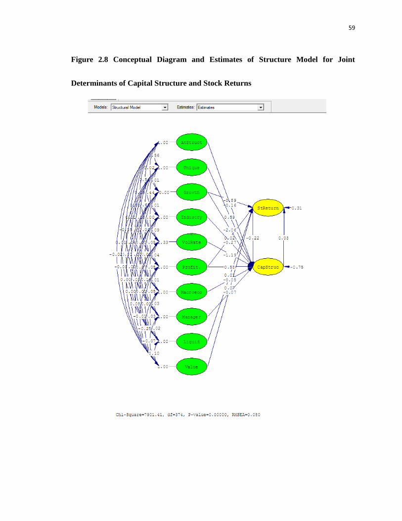
59
Figure 2.8 Conceptual Diagram and Estimates of Structure Model for Joint
Determinants of Capital Structure and Stock Returns
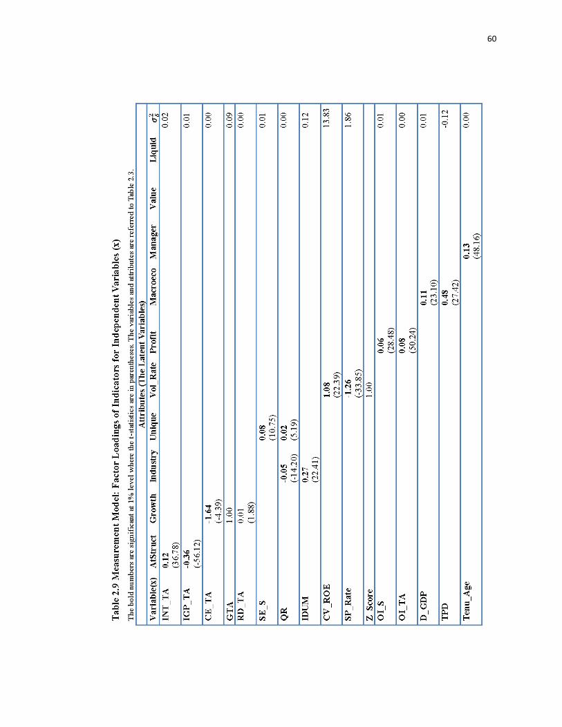
60
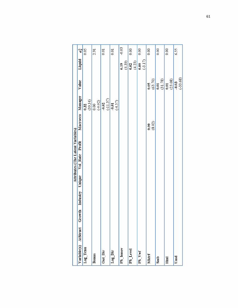
61
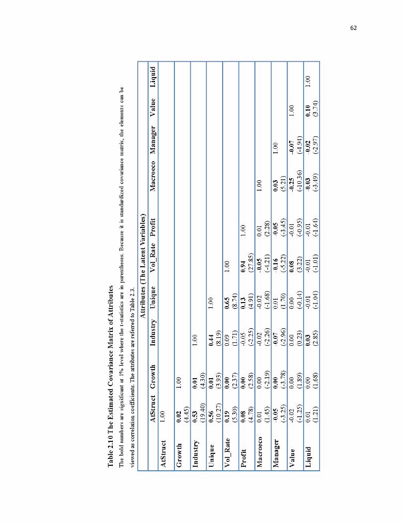
62
63
64
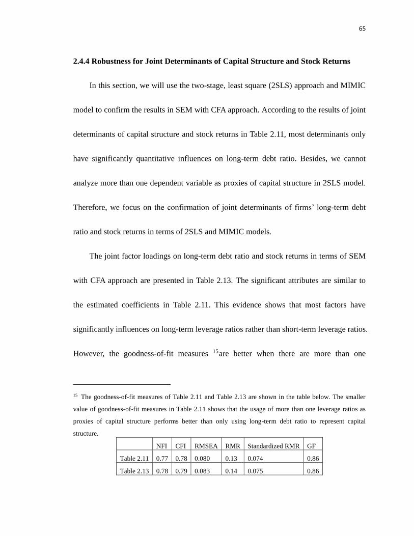
65
2.4.4 Robustness for Joint Determinants of Capital Structure and Stock Returns
In this section, we will use the two-stage, least square (2SLS) approach and MIMIC
model to confirm the results in SEM with CFA approach. According to the results of joint
determinants of capital structure and stock returns in Table 2.11, most determinants only
have significantly quantitative influences on long-term debt ratio. Besides, we cannot
analyze more than one dependent variable as proxies of capital structure in 2SLS model.
Therefore, we focus on the confirmation of joint determinants of firms’ long-term debt
ratio and stock returns in terms of 2SLS and MIMIC models.
The joint factor loadings on long-term debt ratio and stock returns in terms of SEM
with CFA approach are presented in Table 2.13. The significant attributes are similar to
the estimated coefficients in Table 2.11. This evidence shows that most factors have
significantly influences on long-term leverage ratios rather than short-term leverage ratios.
However, the goodness-of-fit measures 15are better when there are more than one
15 The goodness-of-fit measures of Table 2.11 and Table 2.13 are shown in the table below. The smaller
value of goodness-of-fit measures in Table 2.11 shows that the usage of more than one leverage ratios as
proxies of capital structure performs better than only using long-term debt ratio to represent capital
structure.
NFI CFI RMSEA RMR Standardized RMR GF
Table 2.11 0.77 0.78 0.080 0.13 0.074 0.86
Table 2.13 0.78 0.79 0.083 0.14 0.075 0.86

66
leverage ratios to represent capital structure attribute in SEM framework.
In Table 2.14 and 2.15, we can find that the significant factors in 2SLS and MIMIC
models are the same. However, the estimated weights are quite different. We conjecture
that the estimated factor loadings are biased in 2SLS method. That is, the coefficients in
2SLS model are under-estimated because of error-in-variable problem. Therefore, the
estimated coefficients in MIMIC model are larger than it in 2SLS model while the
significant factors in both models are consistent.
The results of robust test show the use of MIMIC model instead of 2SLS model
should be preceded by the elimination of measurement error-in-variable problem in
MIMIC model. However, MIMIC model cannot well identify the influences of factors on
long-term leverage decisions in accordance with capital structure theories. Therefore, I
suggest that the setting of latent attributes to capital structure is necessary when we
investigate the joint determinants of capital structure and stock returns.
67
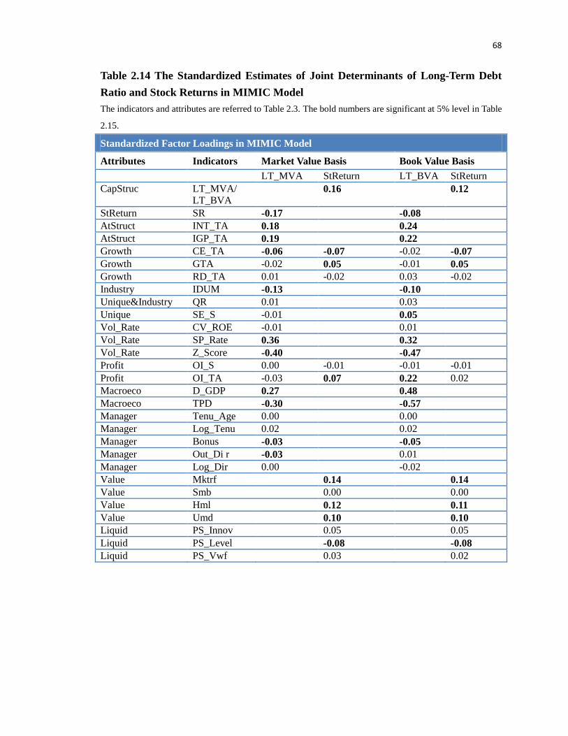
68
Table 2.14 The Standardized Estimates of Joint Determinants of Long-Term Debt
Ratio and Stock Returns in MIMIC Model
The indicators and attributes are referred to Table 2.3. The bold numbers are significant at 5% level in Table
2.15.
Standardized Factor Loadings in MIMIC Model
Attributes Indicators Market Value Basis Book Value Basis
LT_MVA StReturn LT_BVA StReturn
CapStruc LT_MVA/
LT_BVA
0.16 0.12
StReturn SR -0.17 -0.08
AtStruct INT_TA 0.18 0.24
AtStruct IGP_TA 0.19 0.22
Growth CE_TA -0.06 -0.07 -0.02 -0.07
Growth GTA -0.02 0.05 -0.01 0.05
Growth RD_TA 0.01 -0.02 0.03 -0.02
Industry IDUM -0.13 -0.10
Unique&Industry QR 0.01 0.03
Unique SE_S -0.01 0.05
Vol_Rate CV_ROE -0.01 0.01
Vol_Rate SP_Rate 0.36 0.32
Vol_Rate Z_Score -0.40 -0.47
Profit OI_S 0.00 -0.01 -0.01 -0.01
Profit OI_TA -0.03 0.07 0.22 0.02
Macroeco D_GDP 0.27 0.48
Macroeco TPD -0.30 -0.57
Manager Tenu_Age 0.00 0.00
Manager Log_Tenu 0.02 0.02
Manager Bonus -0.03 -0.05
Manager Out_Di r -0.03 0.01
Manager Log_Dir 0.00 -0.02
Value Mktrf 0.14 0.14
Value Smb 0.00 0.00
Value Hml 0.12 0.11
Value Umd 0.10 0.10
Liquid PS_Innov 0.05 0.05
Liquid PS_Level -0.08 -0.08
Liquid PS_Vwf 0.03 0.02
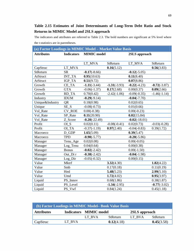
69
Table 2.15 Estimates of Joint Determinants of Long-Term Debt Ratio and Stock
Returns in MIMIC Model and 2SLS approach
The indicators and attributes are referred to Table 2.3. The bold numbers are significant at 5% level where
the t-statistics are in parentheses.
(a) Factor Loadings in MIMIC Model – Market Value Basis
Attributes Indicators MIMIC model 2SLS approach
LT_MVA StReturn LT_MVA StReturn
CapStruc LT_MVA 0.16(5.12) 0.56(3.83)
StReturn SR -0.17(-8.66) -0.12(-5.05)
AtStruct INT_TA 0.95(10.63) 0.11(8.40)
AtStruct IGP_TA 0.51(9.72) 0.07(8.86)
Growth CE_TA -1.11(-3.44) -1.31(-3.93) -0.22(-4.23) -0.72(-3.87)
Growth GTA -0.06(-1.37) 0.17(2.68) 0.00(0.37) 0.09(2.66)
Growth RD_TA 0.70(0.42) -2.42(-1.06) -0.09(-0.35) -1.46(-1.14)
Industry IDUM -0.29(-9.14) -0.04(-7.70)
Unique&Industry QR 0.18(0.98) 0.02(0.65)
Unique SE_S -0.08(-0.73) 0.01(0.66)
Vol_Rate CV_ROE 0.00(-0.38) 0.00(-0.23)
Vol_Rate SP_Rate 0.11(20.90) 0.02(15.84)
Vol_Rate Z_Score -0.20(-22.49) -0.02(-18.01)
Profit OI_S 0.02(0.11) -0.08(-0.41) 0.02(0.73) -0.03(-0.28)
Profit OI_TA -0.37(-1.19) 0.97(2.40) -0.04(-0.83) 0.39(1.72)
Macroeco D_GDP 1.65(5.09) 0.39(5.47)
Macroeco TPD -0.90(-5.77) -0.20(-5.86)
Manager Tenu_Age 0.02(0.08) 0.00(-0.05)
Manager Log_Tenu 0.04(0.64) 0.00(0.38)
Manager Bonus -0.02(-2.42) 0.00(-1.50)
Manager Out_Di r -0.38(-2.42) -0.04(-1.98)
Manager Log_Dir -0.05(-0.32) 0.00(0.15)
Value Mktrf 3.32(4.30) 1.82(4.22)
Value Smb 0.17(0.18) 0.11(0.19)
Value Hml 5.48(5.23) 2.99(5.10)
Value Umd 1.72(4.02) 0.95(3.97)
Liquid PS_Innov 0.68(1.86) 0.38(1.87)
Liquid PS_Level -1.34(-2.95) -0.77(-3.02)
Liquid PS_Vwf 0.84(1.24) 0.45(1.18)
(b) Factor Loadings in MIMIC Model– Book Value Basis
Attributes Indicators MIMIC model 2SLS approach
LT_BVA StReturn LT_BVA StReturn
CapStruc LT_BVA 0.12(4.18) 0.45(3.58)
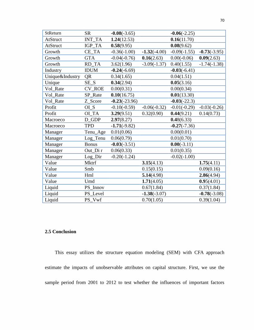
70
StReturn SR -0.08(-3.65) -0.06(-2.25)
AtStruct INT_TA 1.24(12.53) 0.16(11.70)
AtStruct IGP_TA 0.58(9.95) 0.08(9.62)
Growth CE_TA -0.36(-1.00) -1.32(-4.00) -0.09(-1.55) -0.73(-3.95)
Growth GTA -0.04(-0.76) 0.16(2.63) 0.00(-0.06) 0.09(2.63)
Growth RD_TA 3.62(1.96) -3.09(-1.37) 0.40(1.55) -1.74(-1.38)
Industry IDUM -0.24(-6.69) -0.03(-6.41)
Unique&Industry QR 0.34(1.65) 0.04(1.51)
Unique SE_S 0.34(2.94) 0.05(3.16)
Vol_Rate CV_ROE 0.00(0.31) 0.00(0.34)
Vol_Rate SP_Rate 0.10(16.75) 0.01(13.30)
Vol_Rate Z_Score -0.23(-23.96) -0.03(-22.3)
Profit OI_S -0.10(-0.59) -0.06(-0.32) -0.01(-0.29) -0.03(-0.26)
Profit OI_TA 3.29(9.51) 0.32(0.90) 0.44(9.21) 0.14(0.73)
Macroeco D_GDP 2.97(8.27) 0.48(6.33)
Macroeco TPD -1.71(-9.82) -0.27(-7.36)
Manager Tenu_Age 0.01(0.06) 0.00(0.01)
Manager Log_Tenu 0.06(0.79) 0.01(0.70)
Manager Bonus -0.03(-3.51) 0.00(-3.11)
Manager Out_Di r 0.06(0.33) 0.01(0.35)
Manager Log_Dir -0.20(-1.24) -0.02(-1.00)
Value Mktrf 3.15(4.13) 1.75(4.11)
Value Smb 0.15(0.15) 0.09(0.16)
Value Hml 5.14(4.98) 2.86(4.94)
Value Umd 1.71(4.05) 0.95(4.01)
Liquid PS_Innov 0.67(1.84) 0.37(1.84)
Liquid PS_Level -1.38(-3.07) -0.78(-3.08)
Liquid PS_Vwf 0.70(1.05) 0.39(1.04)
2.5 Conclusion
This essay utilizes the structure equation modeling (SEM) with CFA approach
estimate the impacts of unobservable attributes on capital structure. First, we use the
sample period from 2001 to 2012 to test whether the influences of important factors
71
related to accounting information, macroeconomic and manager characters on capital
structure consistent with the literature theories. Then, we investigate the joint
determinants of capital structure and stock rates of returns where we add two attributes,
value and liquidity, to stock returns.
Our empirical work only shows “Profitability” and “Volatility & Financial Rating”
are significant attributes on the decision of capital structure. However, all attributes
become significant determinants of capital structure and stock returns in either market- or
book- value basis. The evidence shows that the interaction of a firm’s leverage and its
stock price should be necessarily considered in capital structure research. Besides the
proof of trade-off between financial distress and agency costs in previous theories, our
results confirm the endogenous supply relationship between public and private debts.
Moreover, the interrelation between leverage ratios and stock returns verifies the signal
theory under the assumption of asymmetric information between managers and investors.
Only significantly negative influence of stock returns on market-value based leverage
ratios supports Welch’s (2004) statement. That is, although stock price is of importance in
dynamic capital structure, a firm would not readjust its capital structure to response the
changes in stock prices.
Finally, we do robustness check by using MIMIC model and the two-stage, least

72
square (2SLS) estimating method. The results show that the factor loadings are
under-estimated in 2SLS approach. Thus, we claim that MIMIC model performs better
because it can solve measurement error-in-variable problem. However, MIMIC model
cannot well identify the influences of factors on long-term leverage decisions in
accordance with capital structure theories. According to comparison of the results in
MIMIC and SEM with CFA models, the setting of latent attributes is necessary to clarify
and confirm theories in capital structure. Therefore, I would suggest using structural
equation modeling (SEM) with confirmatory factor analysis (CFA) to capture the
appropriate factors of firms’ leverage decisions.
In future research, the personal taxes and the differences in beliefs between the
manager and outside investors can be taken account into investigation of joint
determinants of capital structure and stock return (Lin and Flannery, 2013; Yang, 2013).

73
Appendix 2.A: Codes of Structure Equation Modeling (SEM) in LISREL System
(a) Determinants of Capital Structure by SEM with CFA
TI SEM Joint Determinants of Capital Structure and Stock Rate of Return -Only Capital
Structure (Book value)
Observed Variables: V1 V2 V3 V4 V5 V6 V7 V8 V8_1 V9 V10 V11_3 V12
V14 V15 V16_1 V17_1 V18_1 V19_1 V20_1 V21_1 V23 V24 V25 V26 V27
V30 V31 V32 V33 V35_2 V36 V37 V48 V49 V50
Raw data from file Only_capital.psf
sample size = 3118
Latent Variables: AtStruct Nd_tax Growth Uni_Ind Unique Industry Size Vol_Rate Profit
Macroeco Manager CapStruc
Relationships:
V1 V2 =AtStruct
V3 V4 V5=Nd_tax
V6 V7 V23 =Growth
V9 V10 V11_3 = Uni_Ind
V12 V7 =Size
V50 V25 V48 = Vol_Rate
V15 V14 = Profit
V32 V33 V36 V37 V12 = Manager
V27 V31 =Macroeco
V16_1 V17_1 V18_1 =CapStruc
Paths:
AtStruct Nd_tax Growth Uni_Ind Vol_Rate Profit Macroeco Manager Size->
CapStruc
Path Diagram
LISREL Output:ND=4 SC SE SS ME=ML TV AL EF RS AD=off
End of Problem

74
(b) Joint Determinants of Capital Structure and Stock Returns by SEM with CFA
TI SEM Joint Determinants of Capital Structure and Stock Rate of Return -Capital
Structure and Stock return
Observed Variables: NV1-NV45
Raw data from File new_variable_LISREL.psf
sample size = 3118
Latent Variables: AtStruct Unique Growth Industry Vol&Rate Profit Macroeco
Manager Liquid Value StReturn CapStruc
! labal variable only can be read the first 8 character
Relationships:
NV2 NV1 = AtStruct
!NV21 =1.0*Unique
NV10 NV9 =Unique
NV11 NV10 = Industry
NV21 NV6 =Growth
NV7 =1.0*Growth
NV37 NV38 NV39 NV40 =Value
NV34 NV35 NV36 =Liquid
NV14 NV13 =Profit
NV28 NV29 NV32 NV33 NV31 = Manager
NV45 = 1.0*Vol&Rate
NV43 NV23 =Vol&Rate
NV25 NV27 NV37=Macroeco
NV41 = 1.0*StReturn
NV18 - NV20 = CapStruc
set error of NV41 to 0
Paths:
CapStruc Value Liquid Growth Profit -> StReturn
Vol&Rate StReturn Growth Profit Macroeco Manager AtStruct Industry
Unique-> apStruc
Path Diagram
LISREL Output:ND=4 SC SE SS ME=ML TV AL EF RS AD=off
End of Problem

75
Appendix 2.B: Codes of MIMIC Model in LISREL System
(a) Determinants of Capital Structure by MIMIC Model
Raw Data from file MIMICOnly_capital.psf
Sample Size = 3118
Latent Variables CapStruc
Relationships
LT_BVA = CapStruc
ST_BVA = CapStruc
C_BVA= CapStruc
CapStruc = INT_TA SE_S IGP_TA ITC_TA D_TA NDT_TA CE_TA GTA QR
IDUM LnS OI_S OI_TA
CapStruc = RD_A CV_ROE D_GDP TPD Tenu_age log_Tenu Out_Dir log_Dir
SP_Rate
CapStruc = Z_Score INT_TA IGP_TA ITC_TA SE_S
Path Diagram
LISREL Output:ND=4 SC SE SS ME=ML TV AL EF RS AD=off
End of Problem
(b) Joint Determinants of Capital Structure and Stock Returns by MIMIC Model
Raw Data from file new_variable_LISREL.psf
Sample Size = 3118
Latent Variables CapStruc StReturn
Relationships
NV41 = StReturn
NV15 = CapStruc
CapStruc = StReturn
StReturn = CapStruc
CapStruc = NV1 NV2 NV6 NV7 NV21 NV9 NV10 NV11 NV13
CapStruc = NV14 NV23 NV43 NV45 NV25 NV27 NV28 NV29 NV31
CapStruc = NV32 NV33
StReturn = NV6 NV7 NV21 NV13 NV14 NV34 NV35 NV36 NV37
StReturn = NV38 NV39 NV40
Set Error Variance of NV41 To 0.0
Set Error Variance of NV15 To 0.0
Path Diagram
LISREL Output:ND=4 SC SE SS ME=ML TV AL EF RS AD=off
End of Problem
76
CHAPTER 3
Pricing Fair Deposit Insurance: Structural Model Approach
3.1 Introduction
The primary function of a bank is to grant loans to borrowers and receive deposits
from the public. The banks in hence are not only subject to both default and market risks
on the funds they lends, but also to withdrawal risk on the funds they borrowers (O’Hara,
1983). Diamond and Dybig (1983) shows that banks as financial intermediations offer the
demand deposit contracts to increase liquidity by the transformation of illiquid assets into
liquid liabilities. But the deposit contracts may cause real economic damages. During a
bank run, depositors panic and withdraw their deposits immediately because they expect
the bank to fail. Therefore, even a healthy bank can be bankrupt because of the panics of
depositors. In this situation, the bank recalls loans, terminates its investment projects and
then cause real economic damages. Due to maintain the confidence of depositors in banks’
operations, Diamond and Dybig (1983) indicate that the deposit insurance offered from
the government can eliminate the problem of bank runs. Gorton and Pennacchi (1990)
also show that the insured deposit contracts attract uninformed investors who suffer from
trading losses associated with information asymmetries. However, the deposit insurance
77
may bring moral hazard problems. Laeven(2002) argues that depositors have less
incentives to exert and monitor the behavior of banks, and thus banks can tacitly take
excessive risks. VanHoose (2007) asserts that the fair pricing of deposit insurance can
alleviate the moral hazard problems. LeRoy and Singhania (2013), however, conclude
that there is no way to eliminate the moral hazard distortion implied by deposit insurance.
Gan and Wang (2013) state that the necessity and significance of deposit insurance varies
across countries and find that low income countries provide more insurance protection.
Since subprime mortgage crises broke out in August, 2007, pricing fair deposit
insurance premium became an important issue again because the panic of depositors
arose from many financial institutions with financial and liquidity distress. The Federal
Deposit Insurance Corporation (FDIC) should adjust the proper deposit insurance
premium as the trade-off that offsets the costs of bailout plans and the costs of taking
over the deposit account business and partial debt once the financial institutions are
announced bankruptcies. Based on the critical role that insurance deposit risk plays in
financial institutions, the purpose of this project is to investigate the pricing fair value of
deposit insurance.
Regard to the deposit insurance, the insurer must be the government or one of its
agencies such as the FDIC to make the insured deposits as the risk free assets. Deposit
78
insurance guarantees that the promised return will be paid to all who withdraw deposits,
thus it imposes costs on the insurer. Hence an insurer such as the FDIC will receive the
deposit insurance premium as the compensation of the loss of deposit insurance. Blocher,
Seale and Vilim (2003) discuss that the different level of insurance premium received
from banks is based on a risk-based assessment system established by the Federal deposit
insurance corporation (the FDIC). Begin Federal Deposit Insurance Corporation
Improvement Act (FDICIA) of 1991, the first risk-related premium system is categorized
into nine situations which depend on capital levels and supervisory ratings1 (FDIC,
2006). Blocher et al. (2003) shows that the assessment rates of deposit insurance
fluctuated over time in accordance with economic situations. Due to large amounts of
financial institutions’ bankruptcies in subprime mortgage crisis, the FDIC lost enormous
deposit insurance fund to take over bankrupt banks and protect the wealth of depositors.
Therefore, FDIC increased the deposit insurance premium to response the financial
tsunami. This evidence shows that pricing deposit insurance is of importance especially
in financial crisis and should be adjusted in accordance with risk-based scheme (Horvitz,
1 The supervisory ratings are generally based on CAMELS rating. The CAMELS rating is an acronym for
component ratings assigned in a bank examination: Capital, Asset, Management, Earnings, Liquidity and
Sensitivity to market risk. Each component elements has a rating from 1(the best) to 5(the worst), and the
overall composite rating, CAMELS rating, based on these component ratings is then assigned to the bank.
79
1983; Kane 1986). Karas et al. (2013) use Russia banks data to do empirical study and
shows deposit insurance in the presence of a financial crisis can mute depositors’ panic.
Policymaker thereby should be cautioned with respect to the effect of deposit insurance in
financial crisis.
Several models for assessing deposit insurance premium can be grouped into three
main categories: bank failure prediction approach, reduced-form approach, and a
structural approach. The advantage of the bank failure prediction approach is to
determine what variables should be used in a risk-based deposit insurance system (Sinkey,
1975; Avery, Hanweck, and Kwast, 1985). Under this framework, the probability of bank
failure is estimated by the logit model. Hwang, Lee and Liaw (1997) utilize logistic
regressions to identify the financial ratios significantly contributed to bank failures. They
find the financial ratios related to equity capital, profitability and liquidity have
significantly influences on the probability of bank failure. The fair deposit insurance
premium then can be calculated by the probability of failure times the liquidation costs.
Thomson (1991) indicates that the ratio of non-deposit liability to cash and investment
securities significantly affect the bank failure. However, Thomson (1991) states that the
logit estimation is not sensitive to uneven sampling frequencies problem. Thomson (1992)
applies two-step logit regressions to modeling the bank regulator’s closure decision. The
80
first step is the regression of bank’s market value on accounting data, and the second step
is logistic regression to predict bank failure based on the estimated market value of bank
in first step and the constraints on the FDIC’s ability to close insolvent banks.
With regard to reduced-form methodology, Duffie Jarrow, Purnanandam and Yang
(2003) proposed the approach based on reduced-form to price deposit insurance and
claimed this approach need not treat the exact form of the insurance contract because it
does not depend on the liability structure or auditing process of the bank. It is difficult to
capture regulations of an insurance contract within the bank’s capital structure, especially
for banks that are not publicly traded (Falkenheim and Pennacchi, 2003). Duffie et al.
(2003) points out that the fair-market deposit insurance rates can be the product of bank’s
short-term credit spread and the ratio of the insurer’s expected loss at failure per dollar of
assessed deposit to the bond investors’ expected loss at failure per dollar of principal.
Although the reduced-form model can solve the influence of the deposit insurance
contract on evaluation of the deposit insurance premium, there are too many parameters
to be estimated that probably influence the currency of results.
The most studies estimate fair-market FDIC insurance premium by a structural
approach, which typically bases the firm’s asset and the volatility of its asset on its equity
price (Black and Scholes, 1973; Black and Cox, 1976; Merton, 1977, 1978; Leland, 1994;
81
Anderson and Sundaresan, 2000; Bloecher et al. 2003; Brockman and Turle, 2003;
Episcopos, 2008). Merton (1977, 1978) first gives the insight into the relationship
between the deposit insurance and put option. If bank assets cannot meet the amount of
deposits, the bank is insolvent and receives nothing. All remainders of assets belong to
debt holders, that is, depositors. When insolvency of bank occurs, the insurer of deposit
insurance should pay the difference of the bank assets and the deposits to depositors.
Therefore, the contract of deposit insurance can be viewed as a put option written on
bank assets with the strike price equal to deposits. Marcus and Shaked (1984) first
implement Merton’s model to price insurance premium with constant proportional
dividends allowed. Their empirical results show the overpriced deposit insurance
premiums charged by the FDIC.
In the most recent literature, the deposit insurance premium is evaluated by barrier
option models (Brockman and Turle, 2003; Episcopos, 2008). However, the barrier
option model used in previous studies neglects the restrictions of the deposit insurance
contacts. In hence, the structural model approach in terms of the barrier option model and
the Stair Tree model is proposed to deal with bankruptcy costs, the limited
indemnification for depositors, discretely monitoring banks’ situations and the adjustment
of the insurance premium in different financial institution based on a risk-based

82
assessment system. We are then able to build a fair insurance premium system and
calculate the reasonable implied barrier critical points to determine whether FDIC’s
supervisory policy is strict or forbearing.
This paper is organized as follows. In section 3.2, a structural model in terms of
barrier option model and Stair Tree model is illustrated to in accordance with the
restrictions of deposit insurance contracts and bankruptcy costs. The results from the
simulation analysis are discussed in the subsequent section. Finally, section 3.4 includes
the conclusion and the future research.
3.2 The Methodology
At the beginning, the BT model shows the classical structural model, barrier option
closed form, which views the value of equity a down-and-out call (DOC):
DOC(H, X) = VN(a) − Xe−rTN(a − σ√T)
−V(H
V)2N(b) + Xe−rT(
H
V)2−2N(b − σ√T) (3.1)
V is the current market value of bank asset, X is the promised payment to depositors in T
years, H is closure barrier, N is the standard normal cumulative distribution function, and
r is the risk free rate of interest.
Where

83
a =
{
ln(V/X) + (r + σ
2/2)T
σ√T X ≥ H
ln(V/H) + (r + σ2/2)T
σ√T X < 𝐻
b =
{
ln(H
2/VX) + (r + σ2/2)T
σ√T X ≥ H
ln(H/V) + (r + σ2/2)T
σ√T X < 𝐻
= r/σ2 + 1/2
According to capture bank’s equity by DOC, the residual bank’s asset would be
equal to
V − DOC(H, X) = V − C(X) + DIC(H, X)
= Xe−rT − P(X) + DIC(H, X) (3.2)
Where C(X) is a European call option and P(X) is a European put with exercise price X;
DIC (H, X) is a down-and-in call (DIC) with barrier H. The first term is the present value
for the insurants (the depositors) under the full insurance; the last two term is the total
value of FDIC which profits DIC(H,X) by taking over the failure bank but loses P(X) due
to responsibility of insurance payment for depositors at maturity date.
However, BT model is difficult to catch up all real extent of bank regulation, thus
simplifying assumptions, for example, no dividends, no tax, no bankruptcy cost, no
insurance premium, constant volatility and continuous monitor. For example, the contract
of the FDIC deposit insurance is determined quarterly. According to the quarterly
84
financial statement of the financial institutions, the FDIC will receive their insurance
premium by assessing the level of risk-based assessment system. Therefore, the
continuous assumption of the structural model doesn’t seem suitable for the evaluation of
deposit insurances. Another example of the contract’s limitation elaborated in a practical
provision is that the FDIC protects the depositors to a certain extent that the deposit
insurances don’t cover other financial products when a bankruptcy occurs.
Taking the aforementioned into consideration, we provide a novel discretely
structural model based on the Stair Tree model and the concept of BT model to price the
Federal deposit insurance in a barrier option framework. In other words, our extended
structural approach can modify BT model by adding the regulation limitations. This
model not only allows the adjustment of the insurance premium in different financial
institution based on a risk-based assessment system, but also takes account of the loss
from bankruptcy cost and the limited indemnification for depositors. We are then able to
build a fair insurance premium system and calculate the reasonable implied barrier
critical points to determine whether FDIC’s supervisory policy is strict or forbearing.
First of all, the bank asset is only actually monitored discretely at the regular
declaration of financial report and significant announcements. Therefore, we introduce
the concept of the Stair Tree (Dai, 2009) to monitor the bank asset at the auditing time
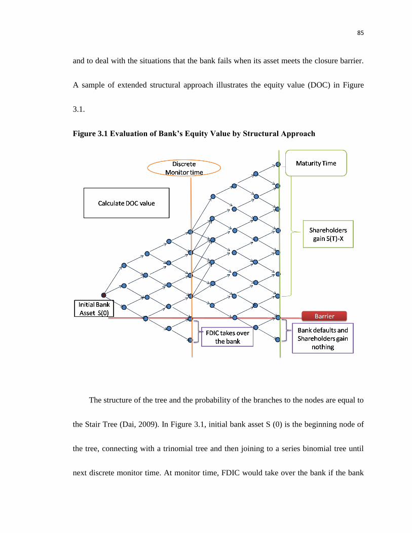
85
and to deal with the situations that the bank fails when its asset meets the closure barrier.
A sample of extended structural approach illustrates the equity value (DOC) in Figure
3.1.
Figure 3.1 Evaluation of Bank’s Equity Value by Structural Approach
The structure of the tree and the probability of the branches to the nodes are equal to
the Stair Tree (Dai, 2009). In Figure 3.1, initial bank asset S (0) is the beginning node of
the tree, connecting with a trinomial tree and then joining to a series binomial tree until
next discrete monitor time. At monitor time, FDIC would take over the bank if the bank
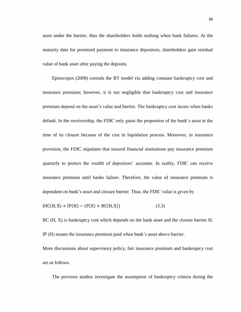
86
asset under the barrier, thus the shareholders holds nothing when bank failures. At the
maturity date for promised payment to insurance depositors, shareholders gain residual
value of bank asset after paying the deposits.
Episocopos (2008) extends the BT model via adding constant bankruptcy cost and
insurance premium; however, it is not negligible that bankruptcy cost and insurance
premium depend on the asset’s value and barrier. The bankruptcy cost incurs when banks
default. In the receivership, the FDIC only gains the proportion of the bank’s asset at the
time of its closure because of the cost in liquidation process. Moreover, in insurance
provision, the FDIC stipulates that insured financial institutions pay insurance premium
quarterly to protect the wealth of depositors’ accounts. In reality, FDIC can receive
insurance premium until banks failure. Therefore, the value of insurance premium is
dependent on bank’s asset and closure barrier. Thus, the FDIC value is given by
DIC(H, X) + IP(H) − (P(X) + BC(H, X)) (3.3)
BC (H, X) is bankruptcy cost which depends on the bank asset and the closure barrier H;
IP (H) means the insurance premium paid when bank’s asset above barrier.
More discussions about supervisory policy, fair insurance premium and bankruptcy cost
are as follows.
The previous studies investigate the assumption of bankruptcy criteria during the

87
period of banks’ auditing time. Under the prompt corrective action (PCA) and closure
rules, that is, bankruptcy occurring when banks fail to meet minimum levels of capital
adequacy, the Federal Deposit Insurance Corporation (FDIC) can take charge of the
banks and be responsible for its liabilities. However, according to the forbearance policy,
the defaulted bank can be allowed to operate under the supervision. With regard to
closure policy, forbearance is granting the bank time to return to solvency before it is
closed. Ronn and Verma (1986) consider that the insurer would infuse funds to the bank
whose asset is below the deposit liability under the forbearing range and then the bank
would not be liquidated immediately. Take account of the forbearing policy into the
framework of option pricing model, Ronn and Verma (1986) state that the deposit
insurance premiums are underestimated. Allen and Saunders (1993) indicate that the
value of the deposit insurance can be viewed as the value of a callable perpetual
American put option under the consideration of forbearance policy. They show that the
deposit insurance premium increases with loose closure policy. Lee, Lee and Yu (2005)
propose the formula for fair deposit insurance and state the fair value of deposit insurance
decreases with the strict policy, which is consistent with the results of Allen and Saunders
(1993).
Since FDIC has the power to set closure policy which makes the deposit insurance
88
contract expire when the bank asset knock the regulatory closure point, the deposit
insurance could be evaluated as a down and out barrier option that the barrier can be
viewed as the regulatory closure rule. Brockman and Turtle (2003) state that the valuation
of the corporate security can be viewed as a path-dependent, barrier option model (BT
model). Episcopos (2008) utilize the BT model to price the deposit insurance premium.
In bank regulation, the value of equity is given by a down-and-out call option with the
barrier as a critical point of failure. In contrast with equity, the FDICs contingent asset
value can be viewed as a down-and-in call option and the FDIC obligation to pay
liabilities, generally deposits, can be viewed as an European put option on written on the
asset of bank. Hwang, Shie, Wang and Lin (2009) modify the barrier option model to
price the deposit insurance by adding the bankruptcy cost as a function of the bank asset
return volatility. They consider the bankruptcy cost explicitly incorporated into the
pricing framework of deposit insurance and make barrier option approach close to
realistic closure policies and regulatory forbearance.
In the basic FDIC deposit insurance contract, the FDIC collects a deposit insurance
premium from each surviving insured financial institution at the beginning of each
quarter. Therefore, it is possible for the FDIC to receive the premium at this quarter but to
take over the failure banks at next quarter with no the deposit insurance premium paid

89
anymore. On the other hand, the assumption is not realistic if structural models assume
continuous monitoring because the accounting information of financial institution only
can be observed quarterly. Besides, in a practical provision, though the FDIC would
cover insurance funds in many kinds of the deposit accounts, including checking and
savings accounts, money market deposit accounts and certificates of deposit (CDs), the
FDIC does not cover other financial products such as stocks, bonds or securities and only
protects each depositor with limitation2.
The purpose of this paper is to combine all above real provisions of the FDIC
contract and to take account of cover limitation of insurance for depositors. Here we
illustrate a simple sample of extended structural approach in Figure 3.2 to implement
FDIC value in reality, concluding insurance premium and bankruptcy cost.
The assumption of insurance premium is paid quarterly as the star sign at the
monitor time and the initial node in Figure 3.2. When bank asset fails to closure barrier,
the FDIC would take over the bank; therefore the value of bank’s shareholders transfers
to FDIC. At this moment, the indirect bankruptcy cost occurs and the bank asset drops
suddenly. At the maturity time, FDIC would gain the profit if the bank asset is enough to
2 Current deposit insurance coverage limit increases from $100,000 to $250,000 per depositor through
December 31, 2009 but unlimited coverage for non-interest bearing transaction accounts. The insurance
coverage limit will return to standard coverage $100,000 for all deposit categories on January 1, 2010.
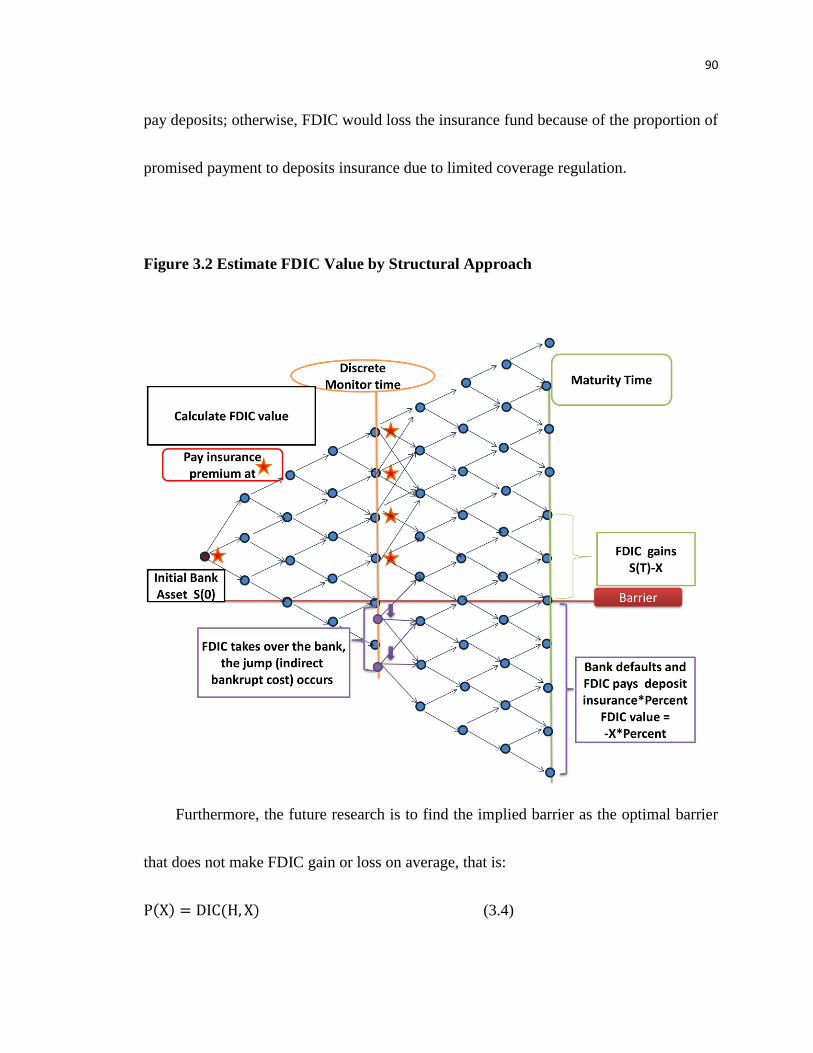
90
pay deposits; otherwise, FDIC would loss the insurance fund because of the proportion of
promised payment to deposits insurance due to limited coverage regulation.
Figure 3.2 Estimate FDIC Value by Structural Approach
Furthermore, the future research is to find the implied barrier as the optimal barrier
that does not make FDIC gain or loss on average, that is:
P(X) = DIC(H, X) (3.4)

91
If we take account of bankruptcy and insurance premium, the determination of implied
barrier follows the equation:
P(X) + BC(H, X) = DIC(H, X) + IP(H) (3.5)
More discussions about supervisory policy, fair insurance premium and bankruptcy
cost are in the future.
3.3 Simulation Results
In this section, we first present the accuracy of our model by the parameters analysis
consistent with the results in BT model. Secondly, moral hazard problem must be
considered due to the relationship between the FDIC value and the level of barrier.
3.3.1 Parameters analysis
Figure 3.3 and Figure 3.4 show the property of convergence in our extended
structural model can accurately generate the value of barrier option in bank capital
regulation (Episcopos, 2008).
Compared with the same parameters in Table 3.1, the value of down-and-out call
options in our numerical approach converges on 15.885 (computed by linear regression)
which close to the value of its closed-form formula (15.8853); the convergent value
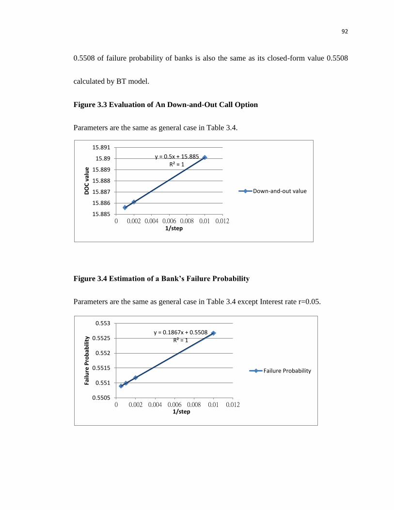
92
0.5508 of failure probability of banks is also the same as its closed-form value 0.5508
calculated by BT model.
Figure 3.3 Evaluation of An Down-and-Out Call Option
Parameters are the same as general case in Table 3.4.
Figure 3.4 Estimation of a Bank’s Failure Probability
Parameters are the same as general case in Table 3.4 except Interest rate r=0.05.
y = 0.5x + 15.885R² = 1
15.885
15.886
15.887
15.888
15.889
15.89
15.891
0 0.002 0.004 0.006 0.008 0.01 0.012
DO
C v
alu
e
1/step
Down-and-out value
y = 0.1867x + 0.5508R² = 1
0.5505
0.551
0.5515
0.552
0.5525
0.553
0 0.002 0.004 0.006 0.008 0.01 0.012
Failu
re P
rob
abili
ty
1/step
Failure Probability
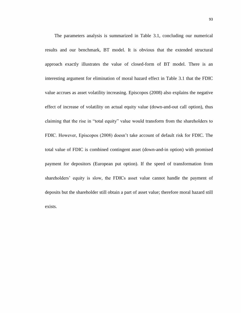
93
The parameters analysis is summarized in Table 3.1, concluding our numerical
results and our benchmark, BT model. It is obvious that the extended structural
approach exactly illustrates the value of closed-form of BT model. There is an
interesting argument for elimination of moral hazard effect in Table 3.1 that the FDIC
value accrues as asset volatility increasing. Episcopos (2008) also explains the negative
effect of increase of volatility on actual equity value (down-and-out call option), thus
claiming that the rise in “total equity” value would transform from the shareholders to
FDIC. However, Episcopos (2008) doesn’t take account of default risk for FDIC. The
total value of FDIC is combined contingent asset (down-and-in option) with promised
payment for depositors (European put option). If the speed of transformation from
shareholders’ equity is slow, the FDICs asset value cannot handle the payment of
deposits but the shareholder still obtain a part of asset value; therefore moral hazard still
exists.
94

95
3.3.2 Moral Hazard Problem
Figure 3.5 and Figure 3.6 show the existence of moral hazard when the supervisory
policy is of forbearance. Figure 3.6, as a part of the cross-section of Figure 3.5,
describes that the FDIC value declines and moral hazard happen under lower barrier
when asset risk increases. In contrast, under higher barrier, the increase of FDIC value
follows the raise of asset risk, that is, the strict supervision policy would diminish moral
hazard.
Figure 3.5 Plot of FDIC Value versus Barrier and Volatility
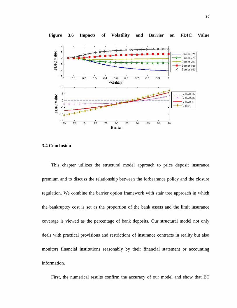
96
Figure 3.6 Impacts of Volatility and Barrier on FDIC Value
3.4 Conclusion
This chapter utilizes the structural model approach to price deposit insurance
premium and to discuss the relationship between the forbearance policy and the closure
regulation. We combine the barrier option framework with stair tree approach in which
the bankruptcy cost is set as the proportion of the bank assets and the limit insurance
coverage is viewed as the percentage of bank deposits. Our structural model not only
deals with practical provisions and restrictions of insurance contracts in reality but also
monitors financial institutions reasonably by their financial statement or accounting
information.
First, the numerical results confirm the accuracy of our model and show that BT

97
model is the special case of our structural model approach. Secondly, the interaction
between closure policy and bankruptcy is incorporated in our model and the results
manifest the important role of bankrupt costs in FDIC supervision. Even though the
increase in regulatory barrier will lead to transfer the wealth from stockholders to the
insurer, the indirectly bankrupt costs will offset this benefit. Therefore, FDIC would
prefer to take forbearance closure policy to protect insurance fund from loss of bankrupt
costs. Finally, the contribution of this chapter is expected to provide the suggestion for
supervisory agencies how to exactly determine a barrier as a policy of taking over
financial institutions. The closure policy for capital regulation can be adjusted by the
setting of insurance premium and the impacts of bankruptcy cost. An appropriate deposit
insurance premium can alleviate potential moral hazard problems caused by a
forbearance policy.
In this essay, we cannot get the information of deposit premium for financial
institutions. Therefore, we cannot test whether the current deposit insurance premium is
overpriced or underpriced. For the future research, if we can obtain real data to find the
fair deposit insurance premium and proper closure barrier, then we can confirm our
presumption. The results are anticipated to consist with our supposition that the
forbearance policy is better than restrict policy for FDIC.

98
CHAPTER 4
Forecasting Implied Volatilities for Options on Index Futures: Time Series and
Cross-Sectional Analysis versus Constant Elasticity of Variance (CEV) Model
4.1 Introduction
Forecasting volatility is crucial to risk management and financial decision for future
uncertainty. Previous studies have found that the volatility changes are predictable (Engle,
1982; Pagan and Schwert, 1990; Harvey and Whaley, 1991, 1992a, 1992b; Day and
Lewis, 1992; Fleming, 1998). In perfectly frictionless and rational markets, options and
their underlying assets should simultaneously and properly change prices to reflect new
information. Otherwise, costless arbitrage profits would happen in portfolios combined
by options and their underlying assets. However, prices in security and option markets
may differently and inconsistently change to respond to news because transaction costs
vary cross financial markets (Phillips and Smith, 1980). Based on trading cost hypothesis,
the market with the lowest trading costs would quickly respond to new information. The
price changes of options on index and options on index futures lead price changes in the
index stocks because trading costs of index option markets are lower than the cost of
trading an equivalent stock portfolio. (Fleming, Ostdiek, and Whaley, 1996). Therefore,

99
the dynamic behavior of market volatility can be captured by forecasting implied
volatilities in index option markets (Dumas, Fleming, and Whaley, 1998; Harvey and
Whaley, 1992a).
In this paper, we use option prices instead of relying on the past behavior of asset
prices to infer volatility expectations of underlying assets. The derivation and use of the
implied volatility (called IV hereafter) for an option as originated by Latane and
Rendleman (1976) has become a widely used methodology for variance estimation. The
IV derived from option prices depends on the assumptions of option valuation formula.
For example, IV in Black-Scholes-Merton option pricing model (called BSM hereafter)
tends to differ across exercise price and times to maturity, which violates the assumption
of the constant volatility of underlying asset in model. The fact that there are as many
BSM IV estimates for an underlying asset as there are options on it, as well as the
observable non-constant nature, has attracted considerable attention from practitioner and
theoretician alike.
For the academician, previous studies have been proposed to capture the
characteristics of implied volatility by either using statistical models or stochastic
diffusion process approaches. Statistical models such as autoregressive conditional
heteroskedasticity (ARCH) models (Engle, 1982) and GARCH model (Day and Lewis,
100
1992) have been used to capture time series nature of IV dynamic behavior. On the other
hand, stochastic process models such as constant-elasticity-of-variance (CEV) model
(Cox, 1975; Cox and Ross, 1976; Beckers, 1980; Chen and Lee, 1993; DelBaen and
Sirakawa, 2002; Emanuel and MacBeth, 1982; MacBeth and Merville, 1980; Hsu, Lin
and Lee, 2008; Schroder, 1989; Singh and Ahmad, 2011; Pun and Wong, 2013; Larguinho
et al., 2013) and stochastic volatility models (Hull and White, 1987; Heston, 1993; Scott,
1997; Lewis, 2000; Lee, 2001; Jones, 2003; Medvedev and Scaillet, 2007) incorporate
the interactive behaviors of an asset and its volatilities in option pricing model. From the
practitioner’s point of view, the implementation and computational costs are the principal
criteria of selecting option pricing models to estimate IV. Therefore, we use
cross-sectional time series regression and CEV model to forecast IV with less
computational costs.
The two alternative approaches used in this paper give different perspective of
estimating IV. The cross-sectional time series analysis focuses on the dynamic behavior
of volatility in each option contracts. The predicted IV obtained from the time series
model is the estimated conditional volatility based on the information of IV extracted
from BSM. Although the estimated IVs in a time series model vary across option
contracts, this kind of model can seize the specification of time-vary characteristic that

101
links ex post volatility to ex ante volatility for each option contract. In addition,
cross-sectional analysis can capture other trading behaviors such as week effect and
in/out of the money effect. On the other hand, CEV model generalizes implied volatility
surface as a function of asset price. It can reduce more computational and implementation
costs rather than the complex models such as jump-diffusion stochastic volatility models
because there is only one more variable compared with BSM. Although the constant
estimated IV for each trading day may cause low forecast power of whole option contacts,
it is more reasonable that the IVs of underlying assets are independent of different strike
prices and times to expiration.
The focuses of this paper are (1) to improve the ability to forecast the IV by
cross-sectional time series analysis and CEV model, (2) to explain the significance of
variables in each approaches, (3) compare prediction power of these two alternative
methods, and (4) test market efficiency by building an arbitrage trading strategy. If
volatility changes are predictable by using cross-sectional time series analysis and CEV
model, the prediction power of these two methods can draw specific implications as to
how BSM might be misspecified. If the abnormal returns are impossible in a trading
strategy which takes transaction costs into account, we would claim that option markets
are efficient.

102
The structure of this paper is as follows. Section 4.2 reviews previous option pricing
models and related empirical works concerning the viability and use of these models. The
data and methodology are described in Section 4.3. Section 4.4 shows the empirical
analysis and devise the trading and hedging strategies to determine if arbitrage profit can
be obtained. Finally, in section 4.5, the implications of the results are summarized from
both an academic and practitioner view.
4.2 Literature Review
The amount of option pricing research is substantial. This section briefly surveys the
major studies which form the impetus for this research effect. Then we introduce
previous literature using time series analysis as an alternative approach to forecast
implied volatilities.
4.2.1 Black-Scholes-Merton Option Pricing Model (BSM) and CEV Model
Option pricing is a central issue in the derivatives literature. After the seminal papers
by Black and Scholes (1973) and Merton (1973), there has been an explosion in option
pricing models developed over the last few decades (Black, 1975; Brenner et al. 1985;
Chance, 1986; Rampini and Viswanathan, 1985; Wolf, 1982, Hull, 2011). BSM formula
for a European call option on a stock with dividend yield rate, q, is:

103
Ct = Ste−qτN(d1) − Ke
−rτN(d2) (4.1)
where d1 =ln(
StK)+(r−q+
σ2
2)τ
σ√τ, d2 = d1 − σ√τ , N(∙) is the cumulative probability
distribution function for a standardized normal distribution, τ is time to maturity, r is
risk free rate, S0 is current underlying stock price, K is exercise price, σ2 is the
variance of stock returns, Ct is the theoretical BSM option price at time t.
Black's (1976) model for pricing futures call options is used in this study. His model is:
1 2
2
1
2 1
[ ( ) ( )]
[ln( / ) ( / 2) ] /
F r
t t
t f f
f
C e F N d KN d
d F K
d d
(4.2)
where CtF is the model price for a call option on future at time t, Ft is the underlying
futures price at time t, K is the exercise price of the call option, τ is the option's remaining
time to maturity in terms of a year, r is the continuous annualized risk-free rate, σf2 is
the instantaneous variance of returns of the underlying futures contract over the
remaining life of the option, and N(∙) is the cumulative normal density function.
The differences in valuing an option on a futures contract versus an option on a
stock can be seen by contrasting Black's model with the BSM. Both models' strengths
rely on the initial establishment of the riskless hedge portfolio between the option, its
underlying asset and some riskless security. However, Black assumes that there are no

104
up-front costs for entering into a futures contract as would occur if one was buying a
stock. Thus in the derivation of the Black models, the interest rate term in the d1 and d2
components of BSM drops out. Additionally, Black implicitly assumes that the futures
price series follows a submartingale; hence the futures price is an unbiased estimation of
the contract's maturity price. It then follows through the derivation that the left hand
portion of equation (4.2) ends up being discounted back to the present at the same rate as
the exercise price (with the additional assumption that the option and futures contracts
mature on the same date). Numerous studies have considered the biasing effects of
dividend payments on the underlying stock which can invoke an early exercise value.
Geske and Roll (1984) found that the American option variant of the BSM formula can
only partially explain the bias associated with the BSM model in the theoretical value of
an option.
While the two pricing models are by no means identical, the general uniformity of
their assumptions and derivations will allow us to concurrently draw direct implications
for the Black model and related but indirect consequences for the BSM option pricing
model. While this paper is concerned primarily with the assumptions that the
instantaneous variance rate is proportionally constant over time, this study also indirectly
examines the model assumptions of a frictionless, liquid market that allows the costless

105
formation and continuous adjustment of riskless hedge portfolios. The costs associated
with low levels of volume are significant in option trading pits, particularly for deep-in
and out-of-the money options and those with a long time to maturity. Evidence of such
costs is exhibited in the wider range of bid-ask prices for these options.
While such a market reality might have some correlation with BSM poorer pricing
performance for such options, a growing array of evidence is emerging which points to
the observed non-constancy of the volatility parameter as a probable source of
misspecification bias. Moreover, the proportionally constant variance and frictionless
markets together imply that an adequately liquid level of trading volume exists for each
option on a particular security. Generally, this implicit condition does not hold in the
market place. As a result of these constraining assumptions, the individual risk-return
characteristics between options differing by exercise price and (or) maturity date, along
with the particular market climate at hand may not be sufficiently expressed in the Black
or BSM model framework.
Empirical tests of the "accuracy" of Black's model are not well founded in the literature,
thus we turn to the abundance of research that has been generated off of the BSM model.
Although it is well known that the BSM model exhibits biases in its pricing of
deep-in and out-of-the-money options and those with a very short or very long term to

106
maturity, the direction of the bias has not been consistent across studies. Black (1975)
found that the BSM model systematically over-priced options which were
deep-in-the-money and underpriced those being deep-out-of-the-money. However,
MacBeth and Merville (1979) reported an exactly opposite type of systematic bias. To
make matters even more imprecise, Merton (1976) notes that practitioners often claim
that the BSM underprices both deep-in and out-of-the-money options. In regards to time
to maturity, it is generally maintained that the BSM underprices short-maturity and
overprices long-maturity options. But again, the evidence contains discrepancies,
particularly when the bias relative to both exercise price and maturity are considered. All
these authors conclude that, to some degree, the pricing bias is related to the volatility
parameter which is typically observed not to be proportionally constant over time.
Jarrow and Rudd (1982) focus on the potential effects from distributional
misspecification of the underlying return-generating process. Thus, their model takes into
account pricing biases which might arise due to differences between the second, third and
fourth moments of the assumed and "true" distributions. Although tests of these models
are far from conclusive, the general impression from the literature is that these models
explain the BSM pricing biases better intuitively than they do empirically. However,
extensive testing and use of these models is somewhat restricted due to the difficulty of
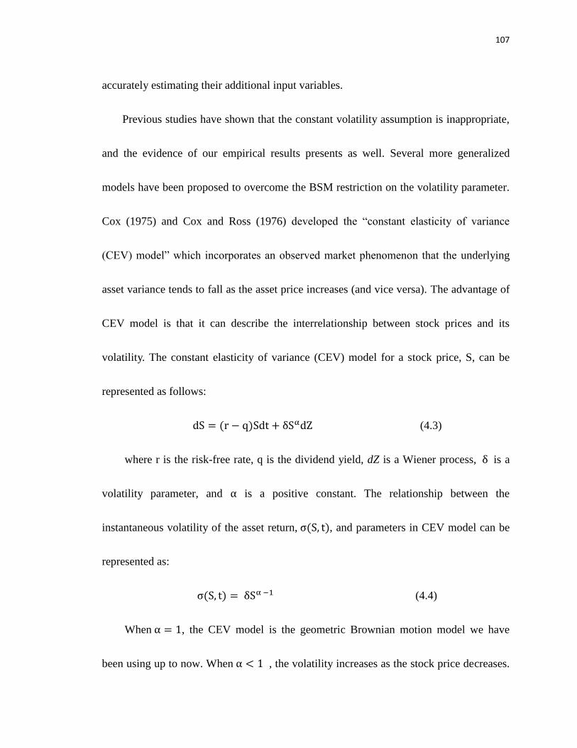
107
accurately estimating their additional input variables.
Previous studies have shown that the constant volatility assumption is inappropriate,
and the evidence of our empirical results presents as well. Several more generalized
models have been proposed to overcome the BSM restriction on the volatility parameter.
Cox (1975) and Cox and Ross (1976) developed the “constant elasticity of variance
(CEV) model” which incorporates an observed market phenomenon that the underlying
asset variance tends to fall as the asset price increases (and vice versa). The advantage of
CEV model is that it can describe the interrelationship between stock prices and its
volatility. The constant elasticity of variance (CEV) model for a stock price, S, can be
represented as follows:
dS = (r − q)Sdt + δSαdZ (4.3)
where r is the risk-free rate, q is the dividend yield, dZ is a Wiener process, δ is a
volatility parameter, and α is a positive constant. The relationship between the
instantaneous volatility of the asset return, σ(S, t), and parameters in CEV model can be
represented as:
σ(S, t) = δSα −1 (4.4)
When α = 1, the CEV model is the geometric Brownian motion model we have
been using up to now. When α < 1 , the volatility increases as the stock price decreases.

108
This creates a probability distribution similar to that observed for equities with a heavy
left tail and a less heavy right tail. When α > 1 , the volatility increases as the stock
price increases, giving a probability distribution with a heavy right tail and a less left tail.
This corresponds to a volatility smile where the implied volatility is an increasing
function of the strike price. This type of volatility smile is sometimes observed for
options on futures.
The formula for pricing a European call option in CEV model is:
Ct = {Ste
−qτ[1 − χ2(a, b + 2, c)] − Ke−rτχ2(c, b, a) when 𝛼 < 1
Ste−qτ[1 − χ2(c,−b, a)] − Ke−rτχ2(a, 2 − b, c) when α > 1
(4.5)
where a =[Ke−(r−q)τ]
2(1−α)
(1−α)2υ, b =
1
1−α, c =
St2(1−α)
(1−α)2υ, υ =
δ2
2(r−q)(α−1)[e2(r−q)(α−1)τ − 1] ,
and χ2(z, k, v) is the cumulative probability that a variable with a non-central
χ2 distribution1 with non-centrality parameter v and k degrees of freedom is less than z.
Hsu, Lin and Lee (2008) provided the detailed derivation of approximative formula for
CEV model. Based on the approximated formula, CEV model can reduce computational
and implementation costs rather than the complex models such as jump-diffusion
stochastic volatility model. Therefore, CVE model with one more parameter than BSM
can be a better choice to improve the performance of predicting implied volatilities of
1 The calculation process of χ2(z, k, v) value can be referred to Ding (1992). The complementary
non-central chi-square distribution function can be expressed as an infinite double sum of gamma function,
which can be referred to Benton and Krishnamoorthy (2003).

109
index options (Singh and Ahmad, 2011).
Beckers (1980) investigate the relationship between the stock price and its variance
of returns by using an approximative closed-form formulas for CEV model based on two
special cases of the constant elasticity class (𝛼 = 1 𝑜𝑟 0). Based on the significant
relationship between the stock price and its volatility in the empirical results, Beckers
(1980) claimed that CEV model in terms of non-central Chi-square distribution performs
better than BC model in terms of log-normal distribution in description of stock price
behavior. MacBeth and Merville (1980) is the first paper to empirically test the
performance of CEV model. Their empirical results show the negative relationship
between stock prices and its volatility of returns; that is, the elasticity class is less than 2
(i.e. 𝛼 < 2). Jackwerth and Rubinstein (2001) and Lee, Wu, and Chen (2004) used S&P
500 index options to do empirical work and found that CEV model performed well
because it took account the negative correlation between the index level and volatility
into model assumption. Pun and Wong (2013) combine asymptotics approach with CEV
model to price American options. Larguinho et al. (2013) compute Greek letters under
CEV model to measure different dimension to the risk in option positions and investigate
leverage effects in option markets.
Merton (1976) derived a model based on a jump-diffusion process for the

110
underlying security that allows for discontinuous jumps in price due to unexpected
information flows. Geske (1979) derived a compound-option formula which considers
the firm's equity to be an option underlying the exchange traded option. An interesting
feature of Geske's model is that by incorporating the effects of a firm's leverage on its
option the model allows for a non-constant variance. Alternative option pricing models to
describe non-constant volatility is stochastic volatility models which consider the
volatility of the stock as a separate stochastic factor (Scott, 1987; Wiggins, 1987; Stein
and Stein, 1991; Heston, 1993; Lewis, 2000; Lee, 2001; Jones, 2003; Medvedev and
Scaillet, 2007). Heston (1993) assumes the dynamics of instantaneous variance, V, as a
stochastic process:
dS = μSdt + √VSdZ1 (4.6a)
dV = (α + βV)dt + σ√VdZ2 (4.6b)
where dZ1 and dZ2 are Wiener processes with correlation ρ. For the complex
implied volatility model without closed-form solutions, advanced techniques such as
partial differential equations (PDEs) or Monte Carlo simulation are used to estimate the
approximation of implied volatility under non-tractable models. Lewis (2000) and Lee
(2001) estimate implied volatility under stochastic volatility model without jumps. Jones
(2003) extends the Heston model and proposes a more general stochastic volatility

111
models in the CEV class as follows:
dS = μSdt + √VSdZ1 (4.7a)
dV = (α + βV)dt + σ1Vγ1dZ1 + σ2V
γ2dZ2 (4.7b)
where dZ1 and dZ2 are independent Wiener processes under the risk-neutral
probability measure. The model setting in Jones (2003) allows the correlation of the price
and variance processes to depend on the level of instantaneous variance. Recently,
Medvedev and Scaillet (2007) deal with a two-factor jump-diffusion stochastic volatility
model where there is a jump term in stock price and volatility follows another stochastic
process related to stock price’s Brownian motion term with constant correlation 𝜌.
Medvedev and Scaillet (2007) empirical results advocate the necessary of introducing
jumps in stock price process. They found that jumps are significant in returns. The
evidence also supports the specification of the stochastic volatility in CEV model (Jones,
2003; Heston, 1993).
The optimal selection of an option pricing model should be based on a trade-off
between its flexibility and its analytical tractability. The more complicated model it is,
the less applicable implementation the model has. Although jump-diffusion stochastic
volatility models can general volatility surface as a deterministic function of exercise
price and time, the computational costs such as parameter calibration or model

112
implementation are high. Chen, Lee and Lee (2009) indicated that CEV model should be
better candidate rather than other complex jump-diffusion stochastic volatility models
because of fast computational speed and less implementation costs. Therefore, we decide
to use CEV model for forecasting implied volatilities in our empirical study.
4.2.2 Time-Varying Volatility and Time Series Analysis
Several studies have attempted to improve the estimation of the volatility term
required by the BSM and Black models. Harvey and Whaley (1992) stated that market
volatility changes are predictable by forecasting the volatility implied in index options.
Their findings are consistent with the trading cost hypothesis that the index futures and
option price changes lead price changes in the stock market (Stephan and Whaley, 1990;
Fleming, Ostdiek, and Whaley, 1996). Therefore, we can employ the predicted IV to do
hedge strategy and risk management.
All the studies involving IV estimation point out to one degree or another that for
any day, the individual IV's for all the options on a particular asset (stock or futures
contract) will all be different, and will change over time. Yet as MacBeth and Merville
(1979) aptly note, different exercise prices should not imply differing IV's since the IV
pertains to the underlying asset itself and not the exercise price. In what might be
considered a preliminary basis for this study, MacBeth and Merville (1979) relate

113
systematic pricing differences between market and BSM option prices to the systematic
differences that occur among individual IV's relative to exercise price and time to
maturity.
Since Latana and Rendleman's (1976) development of the IV concept, numerous
researchers have studied different weighting schemes in calculating the IV. The majority
of studies, including Schmalensee and Trippi (1978) and Chiras and Manaster (1978),
devise weighting schemes which aim at deriving a single weighted IV from among all
individual IV's for input into the BSM model. Whaley (1981; 1982) and Park and Sears
(1985) utilized an OLS regression procedure to weight and segregate IV's by maturity
date. The major finding of the Park and Sears (1985) study, which used option on stock
index futures data, was a "time-to-maturity" effect in the pattern of the weighted IV's
over time. The authors interpreted their findings as being consistent with Merton's (1973)
option pricing model with stochastic interest rate. This is, a portion of the IV's instability
is due to the diminishing instantaneous variance of the riskless security.
Another rather foreshadowing study conducted by Brenner and Galai (1981) not
only found significant divergence between the daily individual IV's and some time series
average IV, but that the distributions of the average IV's were not invariant over time.
Finally, Rubenstein (1985) used individual IV's to test five alternative option pricing

114
models versus the BSM formulation, and attempted to explain observed pricing biases.
Rubenstein (1985) reported that the direction of pricing bias changed over time. This
instability could be a function not only of a time-varying volatility term, but also
stochastic interest rates and a changing stock market climate. Harvey and Whaley (1992)
utilized OLS regression of the change in IV on S&P 100 index option on lagged IV, week
effect dummy variables, and interest rate measures to test if IV is predictable. The
significant abnormal returns obtained in Harvey and Whaley (1992) indicated that the
market volatility is predictable time-varying variable and can be estimated by time-series
analysis.
4.3 Data and Methodology
4.3.1 Data
The data for this study of individual option IV's included the use of call options on
the S&P 500 index futures which are traded at the Chicago Mercantile Exchange (CME)2.
The Data is the options on S&P 500 index futures expired within January 1, 2010 to
December 31, 2013. The reason for using options on S&P 500 index futures instead of
2 Nowadays Chicago Mercantile Exchange (CME), Chicago Board of Trade (CBOT), New York
Mercantile Exchange (NYMEX), and Commodity Exchange (COMEX) are merged and operate as
designated contract markets (DCM) of the CME Group which is the world's leading and most diverse
derivatives marketplace. Website of CME group: http://www.cmegroup.com/

115
S&P 500 index is to eliminate from non-simultaneous price effects between options and
its underlying assets (Harvey and Whaley, 1991). The option and future markets are
closed at 3:15pm Central Time (CT), while stock market is closed at 3pm CT. Therefore,
using closing option prices to estimate the volatility of underlying stock return is
problematic even though the correct option pricing model is used. In addition to no
non-synchronous price issue, the underlying assets, S&P 500 index futures, do not need
to be adjusted for discrete dividends. Therefore, we can reduce the pricing error in
accordance with the needless dividend adjustment. According to the suggestions in
Harvey and Whaley (1991, 1992), we select simultaneous index option prices and index
future prices to do empirical analysis.
The risk free rate used in Black model and CEV model is based on 1-year Treasury
Bill from Federal Reserve Bank of ST. LOUIS3. Daily closing price and trading volumes
of options on S&P 500 index futures and its underlying asset can be obtained from
Datastream.
There are two ways to select data in respect to two alternative methodologies used in
this chapter. For time-series and cross-section analysis, we ignore transaction information
and choose the futures options according to the length of trading period. The futures
3 Website of Federal Reserve Bank of ST. LOUIS: http://research.stlouisfed.org/
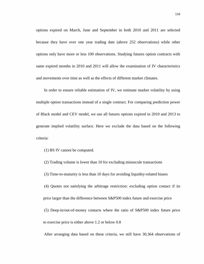
116
options expired on March, June and September in both 2010 and 2011 are selected
because they have over one year trading date (above 252 observations) while other
options only have more or less 100 observations. Studying futures option contracts with
same expired months in 2010 and 2011 will allow the examination of IV characteristics
and movements over time as well as the effects of different market climates.
In order to ensure reliable estimation of IV, we estimate market volatility by using
multiple option transactions instead of a single contract. For comparing prediction power
of Black model and CEV model, we use all futures options expired in 2010 and 2013 to
generate implied volatility surface. Here we exclude the data based on the following
criteria:
(1) BS IV cannot be computed.
(2) Trading volume is lower than 10 for excluding minuscule transactions
(3) Time-to-maturity is less than 10 days for avoiding liquidity-related biases
(4) Quotes not satisfying the arbitrage restriction: excluding option contact if its
price larger than the difference between S&P500 index future and exercise price
(5) Deep-in/out-of-money contacts where the ratio of S&P500 index future price
to exercise price is either above 1.2 or below 0.8
After arranging data based on these criteria, we still have 30,364 observations of

117
future options which are expired within the period of 2010 to 2013. The period of option
prices is from March 19, 2009 to November 5, 2013.
4.3.2 Methodology
In this section, two alternative approaches to estimate IVs are introduced. We first
discuss the algorithm to estimate BSM IVs and illustrate how to obtain BSM IV for each
option contract in MATLAB. Then, based on BSM IVs, we forecast future BSM IVs for
each option contract by time-series analysis and cross-sectional regression. Finally, the
second method to estimate future IV is based on CEV model. To deal with moneyness-
and maturity-related biases, we use the “implied-volatility matrix” to find proper
parameters in CEV model. Then, the IV surface can be represented for predicting future
IV in different moneyness and time-to-maturity categories.
4.3.2.1 Estimating BSM IV
The algorithm to calculate the daily BSM IV for options on S&P 500 index futures
is an important preliminary for IV prediction by cross-sectional time-series analysis. The
examination of IV for each individual option contract, broken down by maturity and
exercise price, is that the estimated IV can be obtained by first choosing an initial
estimate, σ0, and then we use equation (4.8) to iterate towards the correct value as follows:

118
,
, , 0 1 0 0( ) ( )
F
t jF F
t j t j
CC C
(4.8)
where
CFt,j = market price of call option j at time t;
CFt,j (σ0) = theoretical price of call option j at time t given σ = σ0
σ0 = initialized estimate of the IV
σ1 = estimate of the IV from iteration
,
0
F
t jC
= partial derivative of the market price with respect to the standard deviation
evaluated at a σ0
In the context of the Black option pricing model, the partial with respect to the
standard deviation can be expressed explicitly as:
21
, /2( 1)2
F
t j dr r
t t
CFe N d Fe e
(4.9)
where d1 is defined as in equation (4.1). The partial derivative formula in equation (4.9)
is also called Vega of a futures option which is represented the rate of change of the value
of a futures option with respect to the volatility of the underlying futures.
The iteration proceeds by reinitializing σ0 to equal σ1 at each successive stage until an
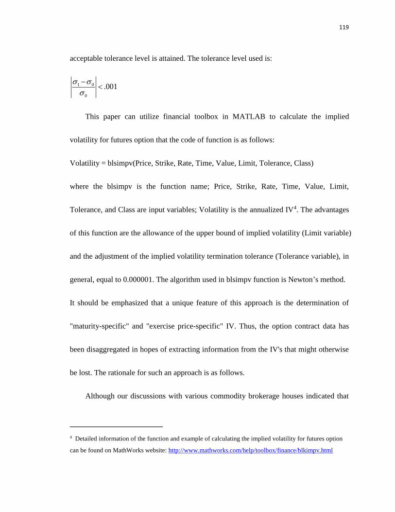
119
acceptable tolerance level is attained. The tolerance level used is:
1 0
0
.001
This paper can utilize financial toolbox in MATLAB to calculate the implied
volatility for futures option that the code of function is as follows:
Volatility = blsimpv(Price, Strike, Rate, Time, Value, Limit, Tolerance, Class)
where the blsimpv is the function name; Price, Strike, Rate, Time, Value, Limit,
Tolerance, and Class are input variables; Volatility is the annualized IV4. The advantages
of this function are the allowance of the upper bound of implied volatility (Limit variable)
and the adjustment of the implied volatility termination tolerance (Tolerance variable), in
general, equal to 0.000001. The algorithm used in blsimpv function is Newton’s method.
It should be emphasized that a unique feature of this approach is the determination of
"maturity-specific" and "exercise price-specific" IV. Thus, the option contract data has
been disaggregated in hopes of extracting information from the IV's that might otherwise
be lost. The rationale for such an approach is as follows.
Although our discussions with various commodity brokerage houses indicated that
4 Detailed information of the function and example of calculating the implied volatility for futures option
can be found on MathWorks website: http://www.mathworks.com/help/toolbox/finance/blkimpv.html

120
most used some type of weighting scheme for IV's, other talks with traders indicated a
preference to consider each option as an individual (derivative) asset. So by utilizing a
conglomerate or maturity-specific IV, those options which are not near-the-money or
moderately close to maturity, will appear to be mispriced. Yet, as other studies have
shown, the BSM and Black models do not price far-in or far-out-of-the-money, or longer
term to maturity options nearly as well as they do the nearer term, near-the-money call
options. As indicated earlier, the assumptions underlying these models do not allow for
market imperfections such as low liquidity and other various market idiosyncrasies. Thus,
the use of weighted IV's would seem to impute a certain degree of "homogenization" into
such options. More specifically, the pricing model used in conjunction with some
weighted IV would not account for such influences as differences in the level or
consistency of volume on the option's actual trading price. Accordingly, all analysis and
interpretation is focused on the IV's of maturity- and exercise price-specific S&P500
index futures options.
When we do the comparison of performance between CEV model and Black model,
the implied volatility of Black model for each group at time t can be obtained by
following steps:
(1) Let Ci,n,tF is market price of the nth option contract in category i, Ci,n,t
F̂ (σ) is the

121
model option price determined by Black model in equation (4.2) with the volatility
parameters, σ. For nth option contract in category i at date t, the difference between
market price and model option price can be described as:
εi,n,tF = Ci,n,t
F − Ci,n,tF̂ (σ) (4.10)
(2) For each date t, we can obtain the optimal parameters in each group by solving
the minimum value of absolute pricing errors (minAPE) as:
minAPEi,t = minσ∑ |εi,n,t
F |Nn=1 (4.11)
Where N is total number of option contracts in group i at time t.
(3) Using MTALAB optimization function to find optimal σ0 in a fixed interval.
The function code is as follows:
[σ0, fvalBls]=fminbnd(fun, x1,x2) (4.12)
Where σ0 is an optimal implied volatility in Black model that locally minimize
function of minAPE, fvalBls is the minimum value of minAPE, fun is MATLAB
function describing equation (4.11). The implied volatility,σ0, is constrained in the
interval between x1 and x2, that is, x1 ≤ σ0 ≤ x2. The algorithm of fminbnd function is
based on golden section search and parabolic interpolation.

122
4.3.2.2 Forecasting IV by Cross-Sectional and Time-Series Analysis
4.3.2.2.1 Time-Series Analysis
Box and Jenkins (1970) time series model building techniques are used to identify,
estimate, and check models describing particular generating processes. These models are
of the form
1 1 1 1t t p t p t t q t qx x x (4.13)
where xt is an observation from a covariance stationary series meaning that
cov( , )t tx x (4.14)
is independent of t for all τ. If stationarity conditions are not satisfied, they can typically
be induced by redefining the xt's to be the first differences between successive
observations. The Φ and θ terms represent the autoregressive (AR) and moving average
(MA) coefficients and εt is white noise. A large body of evidence is accumulating which
supports the Box-Jenkins methodology, especially in cases of single series with moderate
to large numbers of sample observations.
If any stage of the iterative process falls short of being incontrovertibly clear, it is the
initial one. The theoretical relationships between autoregressive moving average
structures and concomitant autocorrelations and partial autocorrelations are often useful
in selecting a model that adequately describes a sample data set. However, detecting

123
these theoretical patterns in practice may be considered more of an art than a science.
A developed technique motivated by Hannan and Rissanen (1982) seems to provide
a good practical basis for model selection. The process involves two stages of
computation. The purpose of the first stage is to obtain estimates of the innovation errors
of model. This is accomplished by running successively higher order auto-regressive
models and using the AIC of Akaike (1969) to determine the optimal order from among
them. The innovation errors are estimated by
1 1ˆ ˆ
t̂ t t k t kx x x (4.15)
where k is the optimal autoregressive order suggested by the AIC. The second stage
involves fitting all different combinations of ARMA (p, q) models where, instead of
using full maximum likelihood estimation, the innovation errors estimated in stage one
are used as the regressors upon which the moving average parameter estimates are based.
This allows use of least squares. The different ARMA (p, q) models are then compared
using the AIC of Akaike (1977) and SBC of Schwarz (1978) and the appropriate model is
chosen on that basis. This procedure comes with no guarantees of consistently being able
to determine "correct" model structures, yet it has been very valuable, when used in
conjunction with sample autocorrelations and partial autocorrelations, in providing good
first guesses.

124
Once the values of p and q are chosen in the initial stage, the parameters are
estimated. A simulation study conducted by Ansley and Newbold (1980) has found that
exact maximum likelihood estimation outperforms least squares when the series are of
moderate size and moving average terms are involved. An approximation to the full
maximum likelihood function has been derived by Hillmer and Tiao (1979).
The fitted models are then subjected to a series of diagnostic checks to ensure that the
initially specified structures are indeed adequate. These checks may be viewed as either
tests against alternative specifications involving additional AR or MA terms or tests
based on the residual autocorrelations from the fitted models.
The sample autocorrelations of each of the IV series were explained they tended to
die out quickly enough over successive lags that the stationarity assumption appears to be
satisfied without first differencing. The series were then modeled in the manner described
above. After satisfactory models were obtained, it remained to find the best use for the
information afforded by the parameter estimates. Certainly the more predictable future
IV's are, the more profitable hedged trading strategies become. In order to test the
accuracy of the ARMA forecasts, the indicators of root mean square error (RMSE), mean
absolute error (MAE) and mean absolute percentage error (MAPE) of recursive updating
forecasts were calculated for holdout periods.

125
In addition, alternative simple time series methods are taken into account to compare
with the forecastability indicators from optimal ARMA models. They are five alternative
models to generate IV indicators which are used in cross-sectional regression model in
next section. These time series models are as follows:
(1) ARMA model (ARMA): IVt = a0 + ∑ aiIVt−ipi=1 + εt + ∑ biεt−i
qi=1
(2) Lag IV method (LIV): IVt = IVt−1
(3) 5-day moving average method (MAV5): IVt =∑ IVt−i5i=1
5
(4) 5-day exponential moving average method (EMA5): IVt =∑ 2i−1IVt−i5i=1
∑ 2i−15i=1
(5) Regression on lag IV (RGN): IVt = a0 + a1IVt−1 + εt
The optimal ARMA model is autoregressive-moving-average model with order of the
autoregressive part, p, and the order of the moving average part, q where the suitable p
and q are based on the goodness-of-fit indicators, AIC and SBC, and the forecastability
indicators, RMSE, MAE and MAPE. The 5-day moving average and the 5-day
exponential moving average methods can be expressed as the special cases of the general
AR(5) model. Lag IV and the regression on lag IV methods belong to AR(1) process.
4.3.2.2.1 Cross-sectional Predictive Regression Model
A significant amount of information has been shown to exist in a time series of IV.
The five alternative time series models used to describe the generating processes of the

126
IV series examined are all clearly preferred to random walk or "white noise" alternatives.
These models do not give the final word on the subject of IV forecasting, however. There
are several cross-contract effects that may exist which, if isolated properly, will provide
further predictive power. To learn more about these different influences, a large
cross-section time series predictive regression model was formulated. The cross-section
time series predictive regression model is
yit = β0 + β1x1it−1 + β2x2it−1 + ••• + β14x14it−1 + εit (4.16)
where
yit = IV of the ith option contract at time t
x1it−1 = the time series predictor of ith contract for time t based on information known
at time t-1 and one of forecasting time-series methods
x2it−1 = time to maturity of the ith option contract at time t-1 which is the unit of year
x3it−1 = proportional in-the-money that is equal to the value of (future price at time t-1 -
strike price)/ (strike price) if the value is positive, otherwise is zero
x4it−1 = proportion out-of-the-money that is equal to the value of (strike price - futures
price at time t-1)/ (strike price) if the value is positive, otherwise is zero
x5it−1 = standard deviation of the IV based on previous 5 observations
x6it−1 = standard deviation of the IV based on previous 20 observations

127
x7it−1 = skewness of IV distribution over the previous 20 observations
x8it−1 = kurtosis of IV distribution over the previous 20 observations
x9it−1 = the standard deviations of the rate of returns of the underlying future price on
previous 5 observations
x10it−1 = the standard deviations of the rate of returns of the underlying future price on
previous 20 observations
x11it−1 = dummy variable that equals 1 if the trading date at time t-1 is Tuesday,
otherwise equal to zero
x12it−1 = dummy variable that equals 1 if the trading date at time t-1 is Wednesday,
otherwise equal to zero
x13it−1 = dummy variable that equals 1 if the trading date at time t-1 is Thursday,
otherwise equal to zero
x14it−1 = dummy, variable that equals 1 if the trading date at time t-1 is Friday,
otherwise equal to zero
The optimal time series predictors are included in an attempt to deduce information
contained in the past. This variable is likely to capture large portions of the expected
cross-contract effects since the market influences pertaining to a particular contract today
are not likely to have changed considerably since the prior trading day. The resulting IV's

128
tend to evolve over time with a strong sense of heritage.
The time-to-maturity variable was included because, as was indicated by Park and
Sears (1985), there tends to be a certain point close to maturity where the IV's begin to
decrease. Of course, any general downward trend in IV's would be partially accounted for
by the ARMA predictors, but it may still be the case that there is a partial influence that
time-to-maturity exhibits. The third and fourth independent variables have been included
to see if deep-in-the-money options and far-out-of-the-money options tend toward higher
or lower than expected IV's. Previous studies have had conflicting answers to this
important question (see Jarrow and Rudd, 1983). The next two independent variables are
included to determine whether or not the standard deviations of the IVs have any positive
or negative effect on the IVs themselves. The third and fourth moments of the
distribution of 20 previous IV observations were also included in the regression equation
to see what, if any, influence they have in determining current IV.
The two measures of the standard deviations of the rate of returns of the underlying
future price are of great interest as regressors since these have traditionally been
approximations of the variable used in the BSM model to determine the theoretical option
price. One would hope to find a strong relationship between the two volatility measures;
the one based on historical deviations and the one implied by the observed option price. It

129
may be the case, however, that the implied standard deviation encompasses more than
just the expected future standard deviation of the underlying asset's return. All BSM
model misspecifications are represented in the IV term, which may amount to quite a
large distortion. A low correlation between these historical and implied variables would
indicate either that the model misspecifications manifesting themselves in the IV terms
are significant or that the historical standard deviation measure is a poor proxy for the
expected future standard deviation, or both.
The final four explanatory variables are weekday effect dummies which are intended
to see if certain days give rise to higher IV than others. For example, certain economic
announcements are regularly made on particular days of the week and this may have a
weekday effect on IV. Note that only four dummy variables are needed to describe the
five days of the week in order to avoid perfect multi-collinearity with the constant term.
4.3.2.3 Forecasting IV by CEV Model
To deal with moneyness- and expiration- related biases in estimating BSM IV, we
use the “implied-volatility matrix” to separate option contracts and estimate parameters
of CEV model in each category. The option contracts are divided into nine categories by
moneyness and time-to-maturity. Option contracts are classified by moneyness level as
at-the-money (ATM), out-of-the-money (OTM), or in-the-money (ITM) based on the

130
ratio of underlying asset price, S, to exercise price, K. If an option contract with S/K ratio
is between 0.95 and 1.01, it belongs to ATM category. If its S/K ratio is higher (lower)
than 1.01 (0.95), the option contract belongs to ITM (OTM) category. According to the
large observations in ATM and OTM, we divide moneyness-level group into five levels:
ratio above 1.01, ratio between 0.98 and 1.01, ratio between 0.95 and 0.98, ratio between
0.90 and 0.95, and ratio below 0.90. By expiration day, we classified option contracts into
short-term (less than 30 trading days), medium-term (between 30 and 60 trading days),
and long-term (more than 60 trading days).
Since for all assets the future price equals the expected future spot price in a
risk-neutral measurement, the S&P 500 index futures prices have same distribution
property of S&P 500 index prices. Therefore, for a call option on index futures can be
given by equation (4.5) with St replaced by Ft and q = r as equation (4.17)5:
CtF = {
e−rτ(Ft[1 − χ2(a, b + 2, c)] − Kχ2(c, b, a) ) when 𝛼 < 1
e−rτ(Ft[1 − χ2(c,−b, a)] − Kχ2(a, 2 − b, c)) when α > 1
(4.17)
where a =K2(1−α)
(1−α)2υ, b =
1
1−α, c =
Ft2(1−α)
(1−α)2υ, υ = δ2τ
5 When substituting q = r into υ =δ2
2(r−q)(α−1)[e2(r−q)(α−1)τ − 1] , we can use L'Hospital's Rule to
obtain υ. Let x = r − q, then
limx→0
δ2[e2x(α−1)τ−1]
2x(α−1)= lim
x→0
∂δ2[e2x(α−1)τ−1]
∂x∂2x(α−1)
∂x
= limx→0
(2(α−1)τ)δ2[e2x(α−1)τ]
2(α−1)= lim
x→0
τδ2[e2x(α−1)τ]
1= τδ2
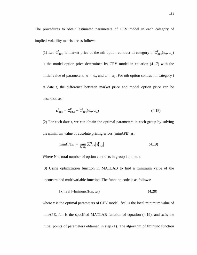
131
The procedures to obtain estimated parameters of CEV model in each category of
implied-volatility matrix are as follows:
(1) Let Ci,n,tF is market price of the nth option contract in category i, Ci,n,t
F̂ (δ0, α0)
is the model option price determined by CEV model in equation (4.17) with the
initial value of parameters, δ = δ0 and α = α0. For nth option contract in category i
at date t, the difference between market price and model option price can be
described as:
εi,n,tF = Ci,n,t
F − Ci,n,tF̂ (δ0, α0) (4.18)
(2) For each date t, we can obtain the optimal parameters in each group by solving
the minimum value of absolute pricing errors (minAPE) as:
minAPEi,t = minδ0,α0
∑ |εi,n,tF |N
n=1 (4.19)
Where N is total number of option contracts in group i at time t.
(3) Using optimization function in MATLAB to find a minimum value of the
unconstrained multivariable function. The function code is as follows:
[x, fval]=fminunc(fun, x0) (4.20)
where x is the optimal parameters of CEV model, fval is the local minimum value of
minAPE, fun is the specified MATLAB function of equation (4.19), and x0 is the
initial points of parameters obtained in step (1). The algorithm of fminunc function

132
is based on quasi-Newton method.
4.4 Empirical Analysis
In the empirical study section, we present the forecastability of S&P 500 index
option price for two alternative models: time-series and cross-sectional analysis and CEV
model. First, the statistical analysis for time-series futures option prices of the contracts
expired on March, June and September in both 2010 and 2011 is summarized. Then we
use time-series and cross-sectional models to analyze each individual contract and
compare their forecastability of IV. Finally, we estimated IV by using CEV model and
compare its pricing accuracy with Black model.
4.4.1 Distributional Qualities of IV time series
One difficulty in discerning the correct value for the volatility parameter in the
option pricing model is due to its fluctuation over time. Therefore, since an accurate
estimate of this variable is essential for correctly pricing an option, it would seem that
time-series and cross-sectional analysis of this variable would be as important as the
conventional study of security price movements. Moreover, by examining individual IV's
over time as well as within different time sets, the unique relationships between the
underlying stochastic process and the pricing influences of differing exercise prices,

133
maturity dates and market sentiment (and indirectly, volume), might be revealed in a way
that could be modeled more efficiently. This section will examine the distributional
qualities of IV's as a prelude to the more quantitatively powerful ARMA and
cross-sectional time series regression models presented in later sections.
A summary of individual IV distributional statistics for S&P 500 index futures call
options in 2010 and 2011 appears in Table 4.1. The most noteworthy feature from this
table is the significantly different mean values of IV's that occur for different exercise
prices. The means and variability of the IV in 2010 and 2011 appear to be inversely
related to the exercise price. More precisely conclusive evidence of the relationship of
IV's to exercise price will arise from the results of the cross-sectional time series
regression in the next section. Comparing the mean IV's across time periods, it is quite
evident that the 2011 IV's are significantly smaller. Also, the time-to-maturity effect
observed by Park and Sears (1985) can be identified. The September options in 2011
possess higher mean IV's than those maturing in June and March with the same strike
price. Once again, stronger support for this effect on the IV's will be displayed in the
regression results.
The other statistical measures listed in Table 4.1 are the relative skewness and
relative kurtosis of the IV series, along with the studentized range. Skewness measures

134
lopsidedness in the distribution and might be considered indicative of a series of large
outliers at some point in the time series of the IV's. Kurtosis measures the peakedness of
the distribution relative to the normal and has been found to affect the stability of
variance (Lee and Wu, 1985). The studentized range gives an overall indication as to
whether the measured degrees of skewness and kurtosis have significantly deviated from
the levels implied by a normality assumption for the IV series.
Although an interpretation of the effects of skewness and kurtosis on the IV series is
postponed until the regression results, a few general observations are warranted at this
point. Both 2010 and 2011 IV’s statistics present a very different view of normal
distribution, certainly challenging any assumptions concerning normality. Using
significance tests on the results of Table 4.1 in accordance with Jarque-Bera test, the
2010 and 2011 skewness and kurtosis measures indicate a higher proportion of statistical
significance. We also utilize simple back-of-the-envelope test based on the studentized
range to identify whether the individual IV series approximate a normal distribution. The
studentized range larger than 4 in both 2010 and 2011 indicates that a normal distribution
significantly understates the maximum magnitude of deviation in individual IV series.
As a final point to this brief examination of the IV skewness and kurtosis, note the
statistics for MAR10 1075, MAR11 1200, and MAR11 1250 contracts. The relative size

135
of this contract's skewness and kurtosis measures reflect the high degree of instability that
its IV exhibited during the last ten days of the contract's life. Such instability is consistent
across contracts.
Table 4.1 Distributional Statistics for Individual IV’s
*Option series contain the name and code of futures options with information of the strike price and the
expired month, for example, SEP11 1350 (B9370V) represents that the futures call option is expired on
September, 2011 with the strike price $1350 and the parentheses is the code of this futures option in
Datastream. **CV represents the coefficient of variation that is standard deviation of option series divided
by their mean value. ***Studentized range is the difference of the maximum and minimum of the
observations divided by the standard deviation of the sample.
Option Series* Mean Std.
Dev.
CV** Skewness Kurtosis Studentized
Range***
Observation
s
Call Futures Options in 2010
MAR10 1075
(C070WC)
0.230 0.032 0.141 2.908 14.898 10.336 251
JUN10 1050
(B243UE)
0.263 0.050 0.191 0.987 0.943 6.729 434
JUN10 1100
(B243UF)
0.247 0.047 0.189 0.718 -0.569 4.299 434
SEP10 1100
(C9210T)
0.216 0.024 0.111 0.928 1.539 6.092 259
SEP10 1200
(C9210U)
0.191 0.022 0.117 0.982 2.194 6.178 257
Call Futures Options in 2011
MAR11 1200
(D039NR)
0.206 0.040 0.195 5.108 36.483 10.190 384
MAR11 1250
(D1843V)
0.188 0.027 0.145 3.739 25.527 10.636 324
MAR11 1300
(D039NT)
0.176 0.021 0.118 1.104 4.787 8.588 384
JUN11 1325
(B513XF)
0.165 0.016 0.095 -1.831 12.656 10.103 200
JUN11 1350
(A850CJ)
0.161 0.018 0.113 -0.228 1.856 8.653 234
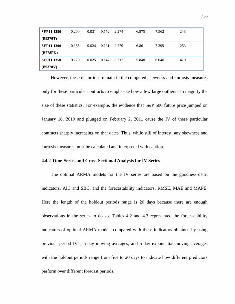
136
SEP11 1250
(B9370T)
0.200 0.031 0.152 2.274 6.875 7.562 248
SEP11 1300
(B778PK)
0.185 0.024 0.131 2.279 6.861 7.399 253
SEP11 1350
(B9370V)
0.170 0.025 0.147 2.212 5.848 6.040 470
However, these distortions remain in the computed skewness and kurtosis measures
only for these particular contracts to emphasize how a few large outliers can magnify the
size of these statistics. For example, the evidence that S&P 500 future price jumped on
January 18, 2010 and plunged on February 2, 2011 cause the IV of these particular
contracts sharply increasing on that dates. Thus, while still of interest, any skewness and
kurtosis measures must be calculated and interpreted with caution.
4.4.2 Time-Series and Cross-Sectional Analysis for IV Series
The optimal ARMA models for the IV series are based on the goodness-of-fit
indicators, AIC and SBC, and the forecastability indicators, RMSE, MAE and MAPE.
Here the length of the holdout periods range is 20 days because there are enough
observations in the series to do so. Tables 4.2 and 4.3 represented the forecastability
indicators of optimal ARMA models compared with these indicators obtained by using
previous period IV's, 5-day moving averages, and 5-day exponential moving averages
with the holdout periods range from five to 20 days to indicate how different predictors
perform over different forecast periods.
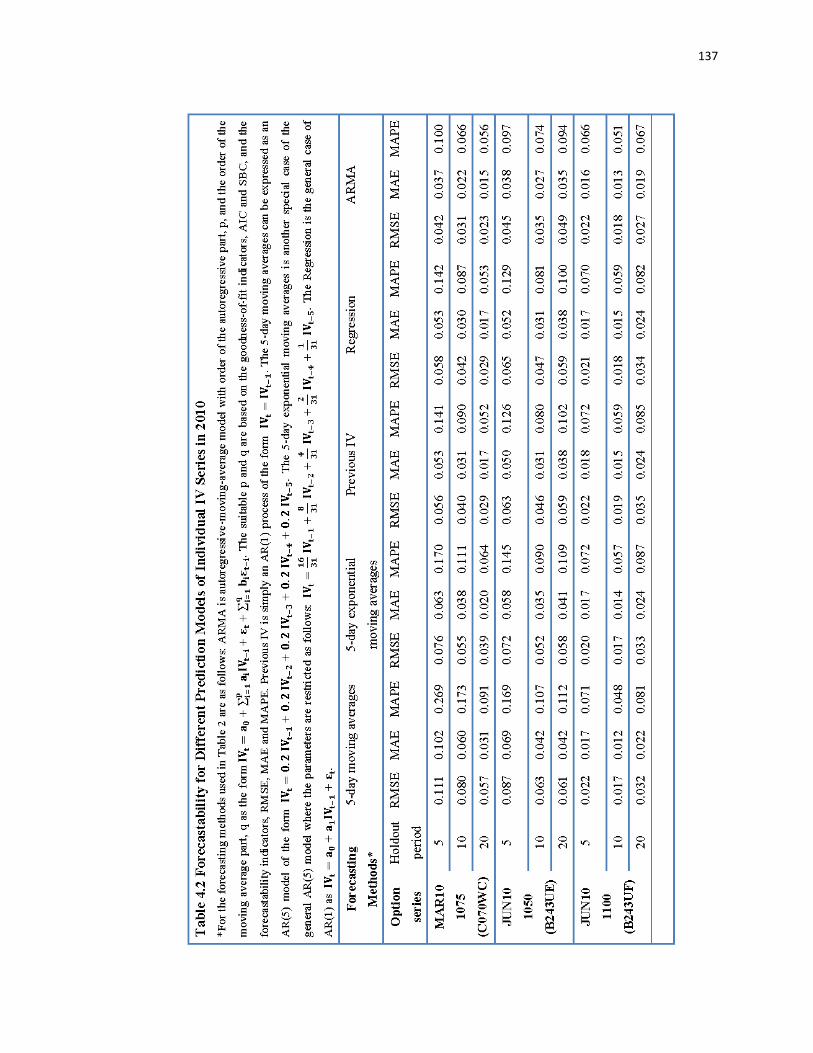
137
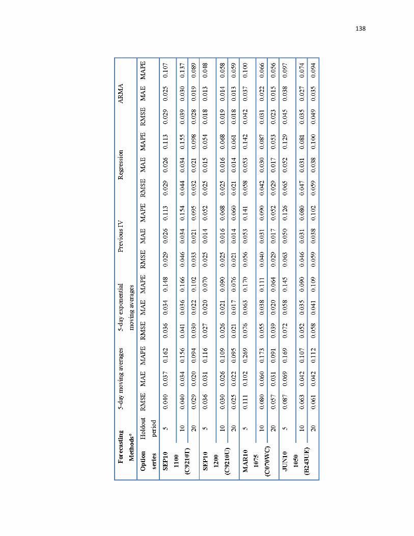
138

139
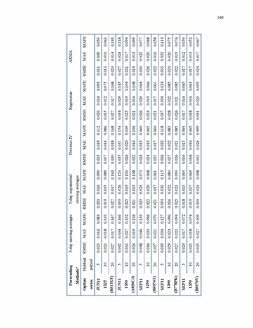
140

141
As Tables 4.2 and 4.3 indicate, the superior forecasting method is ARMA model
based on the smallest value of RMSE, MAE, MAPE except that the previous IV method
predict better than ARMA for SEP11 1250 contract. The better prediction ability of
ARMA method is attributed to the same characteristic of other alternatives forecasting
methods that are considered are actually specific cases of ARMA models themselves
where the structural and quantitative relationships of the time series with their forecasts
are predetermined. The efficiently specified and estimated ARMA models are chosen on
the basis of the data and would therefore be expected to better project particular data
generating processes into the future. The best explanation for the poorer prediction
performance of ARMA model for SEP11 1250 contract is that the forecast periods, at
times, exhibit structural change or even a sudden trend in IV's. Non-stationarity (trend
behavior) was not observed in the estimation period and hence the ARMA coefficients
that were derived for that time could not predict any stationarity in the holdout period.
Some of the other, "naive" fore-castors are more responsive to these sudden movements.
They do not have as much of a tendency to pull their forecasts toward middle ground as
ARMA models do. For example, the most naive forecast in the previous IV method
(i.e., IVt = IVt−1 ) will be better than some ordinarily superior ARMA forecast in
regression method (i.e., IVt = a0̂ + a1̂IVt−1) in times of unanticipated non-stationarity.

142
The forecasts were also compared with those derived from the regression model
developed in the following section.
To tie together some of the results identified thus far, observe the interesting
relationship that arises from an examination of RMSE, MAE, MAPE from the ARMA
forecasts as shown in Tables 4.2 and 4.3, and the standard deviations of the IV series as
shown in Table 4.1. While not precise, it is apparent that the accuracy of the ARMA
forecasts correlates with the variability of the IV series. Hence, the more volatile the IV,
the more difficult it is to forecast. While this observation might be obvious, a further
implication is suggested. For instance, one could find such information valuable in
deciding which particular options might be mispriced based on the use of the BSM (or
Black’s) option pricing model and some forecast of the IV. For example, if the
forecasting models show that both SEP11 1300 and SEP11 1350 options are underpriced
and SEP11 1350 option has a significantly lower standard deviation than the other one,
we might confidently state that SEP11 1350 option is mispriced rather than SEP11 1300
option.
Determining the correct form of a model using pooled cross-section and time series
data is an important, though often troublesome task. The difficulty arises because the
error term may consist of time-series-related disturbances, cross-section disturbances, or

143
both. The regression equation is defined with the time series predictor calculated by one
of five forecasting methods in the design matrix. This insures that any possibility of
autocorrelation in the time series disturbances has been mitigated. There remains the
chance that contemporaneous correlation of disturbances across contracts exists.
However, a majority of this cross-contract relationship will be accounted for by the
in-the-money and out-of-the-money variables. These are akin to the cross-section dummy
variables of the so-called covariance model. The only real difference between the two
sets of variables is that the estimated dummy coefficients can take on any values whereas
the in-the-money and out-of-the-money variables implicitly assume that a linear
relationship exists between a contract's strike price above the underlying asset price and
its IV and between a contract's strike price below the underlying asset price and its IV. If
this posited linear relationship does exist, then cross-contract disturbances should not be
highly correlated. The proper estimation procedure is ordinary least squares. Of course,
the residuals must be checked for possible violations of the assumptions before placing
confidence in the sample results.
Table 4.4 shows the results of the regression model in equation (4.16). The time
series predictor variables calculated by different forecasting models are all significant,
which should come as no surprise—IV depends on past IV value. However, the fact that

144
other regressors were found to be significant indicates that not all of the variation in IV
series is explained by the past. Time-to-maturity has the predicted positive effect. The
closer an option is to expiration, the lower the IV. The in-the-money effect is
significantly positive; however, the out-of-the-money give mixed insignificant influence
on IV series. Merton (1976) shows that large deviations from the strike price tend to bias
the BSM theoretical price downward. Therefore it is logical to expect the IV of the
deep-in-the-money and far-out-of-the-money contracts to be higher because the writer of
these calls runs a greater risk of being stuck in his position. However, in this study, the
selected IV time series calculated by BSM model cannot show the downward
characteristic obviously because the longest trading data is the option contract with the
strike price close to the underlying asset.
The coefficients on the standard deviation of the IV variables give the significantly
positive signals based on previous 20 observations, but show the negative effect based on
previous 5 observations when the short term effect is of significance. The skewness and
kurtosis terms have consistently slight effects over two sample periods even though
sometimes the effects have statistical significance. Perhaps what can be said about the
lower relationship between these two statistic measures and predicted IV is that the
influence of the outliers bringing about the skewness and kurtosis is already captured by

145
other independent variables such as the time series predictor estimated by forecasting
model or the standard deviation of IV series.
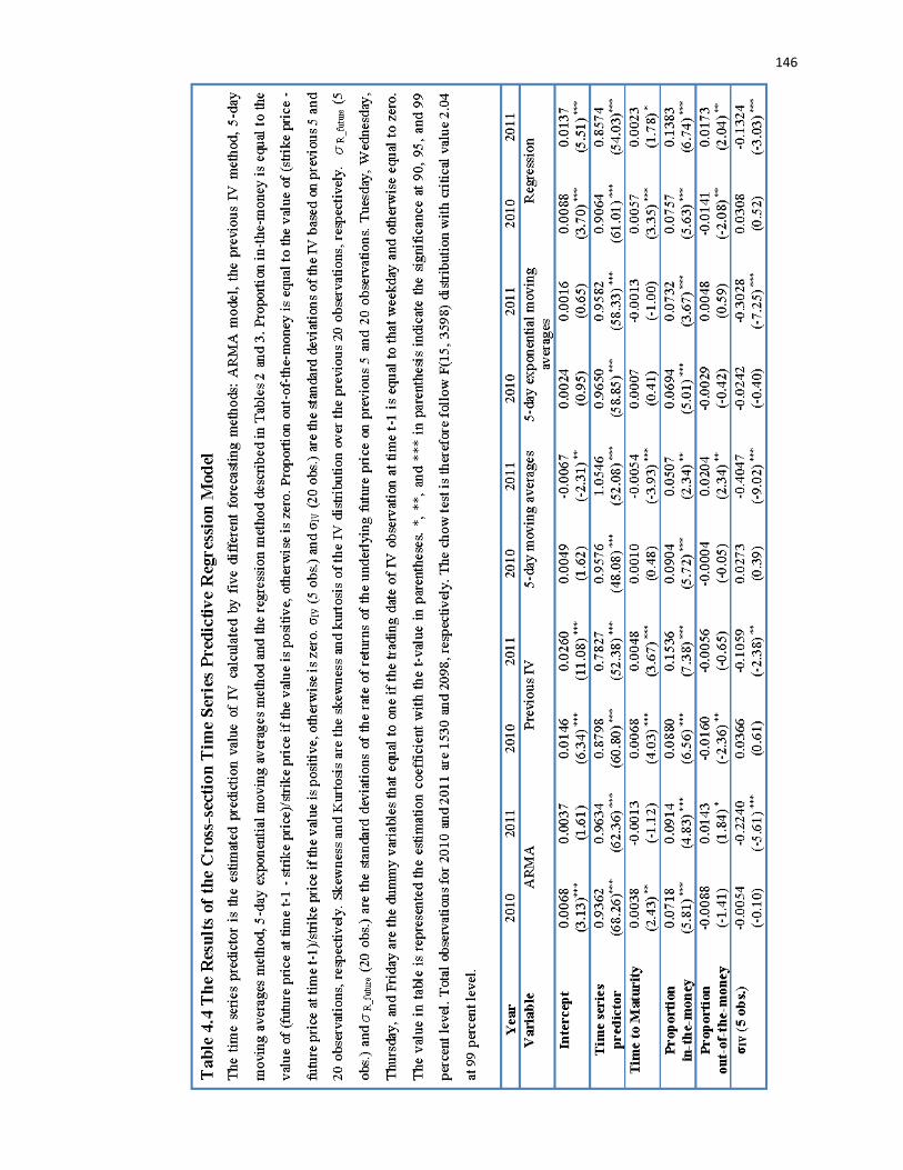
146
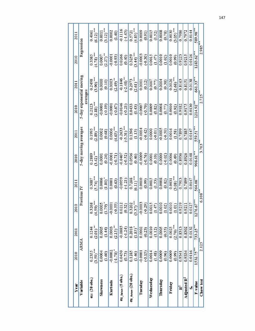
147

148
The coefficient on the standard deviation of the rate of returns of the underlying
future price only has significantly large positive effect on IV for the 20-day measure. The
strong relationship to historical standard deviations of underlying assets seems that the IV
series not only response to market deviation from the functional specification of the BSM
model but also reflect the market assessment of the standard deviation of underlying
assets.
The weekday effect dummies indicate a significantly small Friday effect where the
IV are slightly higher. This may be related to the fact that certain economic
announcements are made on Friday such as employment situation or lag response to the
announcements made on Thursday such as money supply and jobless claims. These
economic announcements will alter the market perception of asset price volatility,
especially currently the situation of economics that just came through the financial crisis
and is suffering from European sovereign-debt crisis. The Friday effect might also be
related to option market inactivity the day before the weekend. Further study may
investigate this apparent weekday effect to explain why Friday's market may be out of
line with that of other days.
Whether the estimated models change significantly over time is an important
149
question. The parameter estimates obtained for this cross-section time series model seems
not consistent in 2010 and 2011 sample periods. A Chow test6 statistic indicating
structural change based on five forecasting methods are obtained in Table 4.4 for the
2010 and 2011 regressions and are calculated to be 2.125, 6.108, 3.763, 2.725 and
2.985,respectively .These values exceed the table value of 2.04 for an F random variable
at the 99 percent level. The chow test indicated the significant change of structure in the
cross-section time series predictive regression model on 2010 and 2011. It would
therefore be wise for the practitioner to update parameter estimates periodically even
though both 2010 and 2011 sample periods are suffering from global financial crisis.
4.4.3 Ex-Post Test for Forecastability of Time-Series and Cross-Sectional Regression
Models
In the previous section, the various estimated methods such as ARMA and
regression models for the "true-future" underlying IV are compared to a number of naive
methods and evaluated through the conventional measure of forecast accuracy such as
RMSE, MAE and MAPE. Now the practical monetary value of the IV estimates versus
more naive methods is tested, to determine which might be superior from a trader's point
6 Chow test 𝐹𝑞,𝑛−𝑘 =𝑒∗′ 𝑒∗/𝛼
𝑒 ′𝑒/(𝑛−𝑘) where 𝑒∗
′𝑒∗ is restricted SSE, 𝑒 ′𝑒 is unrestricted SSE, 𝛼 represents the
number of restrictions, and k is number of regression coefficients estimated in unrestricted regression.

150
of view. In addition, we hope that these results will further support the theoretical and
practical superiority of using individual IV estimates versus some weighted-IV measure.
Discussions with traders of options on S&P 500 index futures along with various
segments of the brokerage industry yielded a general view of how IV's are utilized in
practice. The common methods are to look at yesterday's weighted-IV (though some
sources indicated that they looked at individual IV's), or some type of moving average
scheme of past IVs as being the true-future underlying volatility to use in the Black
option pricing model. Changes in the option price due to the deviation in the current IV
from the estimates of the true-future IV is thus deemed as mispricing by the market.
Trading rule tests in this paper utilizes seven different estimates for IV as follows:
(1) a 5-day equally-weighted moving average of the IV (MAV5)
(2) a 5-day exponentially-weighted average of the IV (EMA5)
(3) a 1-day lag of the actual IV for the option (LIV)
(4) 1-day ahead simple regression forecasts of the IV (RGN)
(5) 1-day ahead ARMA forecasts of the IV (ARMA)
(6) 1-day ahead cross-section time series predictive regression forecasts of the IV
based on equation (4.16) (CSTS)
(7) a simple-constant mean of an individual IV time series for the estimated IV of

151
that option (MEAN)
The trading rule used is simply to buy underpriced and sell overpriced options, while
taking an opposite position in the underlying futures contract according to the hedge ratio
computed by the estimated IV. The holdout periods for each option are twenty trading
days. Here the day count convention in Black option pricing model is used actual/actual
basis. Mispricing will be identified by comparing the market price for an option with the
price calculated by Black option pricing model using one of the seven IV estimates. The
overpriced (underpriced) options are defined as the situation that the theoretical price
calculated by Black option pricing model is smaller (larger) than the market price. The
trading behavior is buying (selling) the underpriced (overpriced) future option and selling
(buying) S&P 500 index future for hedge. In order to magnify the mispricing as might be
seen from the eyes of a trader, ten options and ten times the hedge ratio of futures are
sold or bought in opposite position respectively in each transaction. Positions are closed
out once the absolute value of mispricing diminishes to a predetermined minimum level
equal to 0.1. If the mispricing has reversed and is of a great enough significance larger
than 0.1, the trading rule is utilized again.
In order to ascribe as much realism as possible to these tests, the following market trading
costs are considered. Transaction fee per transaction of $2.3 is determined by CME group

152
which provides CME Globex trading platform for 24-hour global access to electronic
markets. These costs were calculated as follows:
Total transaction fees
= transaction costs of option position + transaction costs of future position
= 1 1
($2.3 10) ($2.3 10 hedge ratio )i
n n
T
i i
where n is the total number of times a position is opened at time Ti .
Although a portion of the margin required of a trader enter into a futures position
can be put up in the form of interest earning T-bills, a substantial portion required for
maintaining the margin account by the clearinghouse must be strictly in cash even for a
hedge or spread position. Consequently, there is a real interest cost involved, for which
we will further reduce gross trading income:
1
Margin Interest Costs ( )i i
n
T T i
i
RMM NF R
where RMM is required maintenance margin from CME group7, NFTi indicate the
number of futures contracts entered into trading which is equal to ten times hedge ratio at
7 The minimum required maintenance for S&P 500 index futures is various in different period. For
example, from Jan 28, 2008 to Oct 1st, 2008, the maintenance cost is $18,000 per future contract. However,
the period during Oct 1st, 2008 to Oct 17, 2008, the required maintenance is changed to $20,250. The
maintenance costs are $22,500, $24,750, $22,500, and $20,000 for other periods Oct 17, 2008-Oct 30,
2008; Oct 30, 2008-Mar 20, 2009; Mar 20, 2009-Jun 2nd, 2011; and Jun 2nd, 2011 until now.

153
time Ti, RTi is the risk free rate defined as the 3-month T-bill rate used in Black option
pricing model, τi is the length of futures position holding until maturity in annual terms,
and n is the total number of times a futures position is entered.
Other very real and significant market costs are those associated with liquidity and
timing. Options which are deep-in-the-money for instance, are not heavily traded and
therefore present additional costs for actually getting into or out of a position. Since the
last reported price for the option may not have occurred at the same time as that for the
underlying future, there always arises a problem with using closing prices. Furthermore,
there is little assurance that one could buy or sell these contracts and expect to receive the
closing prices reported in the paper when the market reopens the next morning. To
approximate such market costs the position is penalized each time a futures position is
entered and existed by "one tick" equal to 0.1 index points = $25 per contract8:
1
Futures Liquidity Costs ($50 )i
n
T
i
NF
where $50 = 2 × $25 represented the entered and existed cost by one tick, the market
value of two price ticks; NFTi is defined as the number of futures contracts entered into
trading which is equal to ten times hedge ratio at time Ti,, and n is the number of times a
8 The detailed contract specifications for S&P 500 futures and options on futures can be found in CME
group website: http://www.cmegroup.com/trading/equity-index/files/SxP500_FC.pdf
154
futures position is entered.
More severe liquidity and timing costs are calculated and deducted for each option
transaction:
1
Option Liquidity costs [$250 (NEPA NMMO )]i
n
T T i
i
where $250 = 10, (number of options bought or sold) × $250 (the market value multiplier
for the option premium) × 0.1 (one tick price as the correspondingly liquidity), NEPA
represented the number of exercise prices in out-of-the-money options are $5 away from
underlying future prices at time Ti, and NMMO represented the percentage of maturity
months out. For example, a option assumed to be expired on September 2010 and this
option start to be traded on February 2010, then the NMMO on June 2010 is equal to the
number of month of the period between February and June divided by the number of
month of the period between February and September, that is, (6-2)/(9-2)=4/7.
The test results are summarized in Tables 4.5 through 4.7. We use seven alternative
methods, a cross-sectional time-series regression and six time series models, to compute
tomorrow’s IV for each contract. The cross-section time series (CSTS) model utilized
some of the insights of time series analysis as would be impounded in the optimal time
series predictors, ARMA model. Also, it takes into account the historical 5-days and
20-days standard deviation of the continuous return for the underlying futures contract,
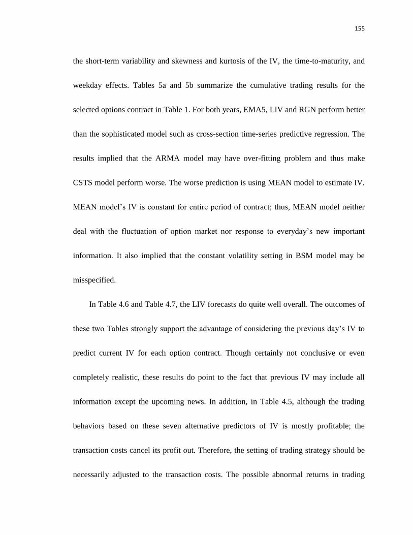
155
the short-term variability and skewness and kurtosis of the IV, the time-to-maturity, and
weekday effects. Tables 5a and 5b summarize the cumulative trading results for the
selected options contract in Table 1. For both years, EMA5, LIV and RGN perform better
than the sophisticated model such as cross-section time-series predictive regression. The
results implied that the ARMA model may have over-fitting problem and thus make
CSTS model perform worse. The worse prediction is using MEAN model to estimate IV.
MEAN model’s IV is constant for entire period of contract; thus, MEAN model neither
deal with the fluctuation of option market nor response to everyday’s new important
information. It also implied that the constant volatility setting in BSM model may be
misspecified.
In Table 4.6 and Table 4.7, the LIV forecasts do quite well overall. The outcomes of
these two Tables strongly support the advantage of considering the previous day’s IV to
predict current IV for each option contract. Though certainly not conclusive or even
completely realistic, these results do point to the fact that previous IV may include all
information except the upcoming news. In addition, in Table 4.5, although the trading
behaviors based on these seven alternative predictors of IV is mostly profitable; the
transaction costs cancel its profit out. Therefore, the setting of trading strategy should be
necessarily adjusted to the transaction costs. The possible abnormal returns in trading
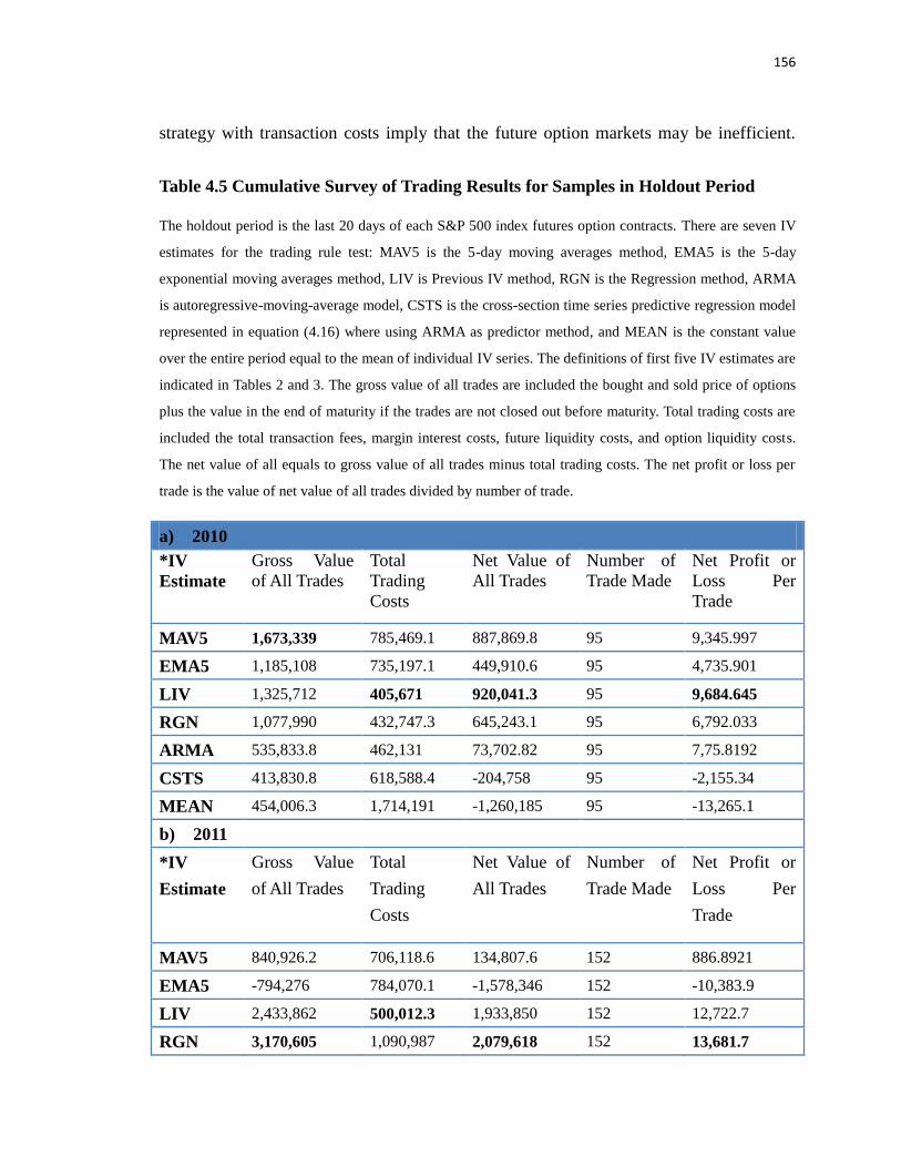
156
strategy with transaction costs imply that the future option markets may be inefficient.
Table 4.5 Cumulative Survey of Trading Results for Samples in Holdout Period
The holdout period is the last 20 days of each S&P 500 index futures option contracts. There are seven IV
estimates for the trading rule test: MAV5 is the 5-day moving averages method, EMA5 is the 5-day
exponential moving averages method, LIV is Previous IV method, RGN is the Regression method, ARMA
is autoregressive-moving-average model, CSTS is the cross-section time series predictive regression model
represented in equation (4.16) where using ARMA as predictor method, and MEAN is the constant value
over the entire period equal to the mean of individual IV series. The definitions of first five IV estimates are
indicated in Tables 2 and 3. The gross value of all trades are included the bought and sold price of options
plus the value in the end of maturity if the trades are not closed out before maturity. Total trading costs are
included the total transaction fees, margin interest costs, future liquidity costs, and option liquidity costs.
The net value of all equals to gross value of all trades minus total trading costs. The net profit or loss per
trade is the value of net value of all trades divided by number of trade.
a) 2010
*IV
Estimate
Gross Value
of All Trades
Total
Trading
Costs
Net Value of
All Trades
Number of
Trade Made
Net Profit or
Loss Per
Trade
MAV5 1,673,339 785,469.1 887,869.8 95 9,345.997
EMA5 1,185,108 735,197.1 449,910.6 95 4,735.901
LIV 1,325,712 405,671 920,041.3 95 9,684.645
RGN 1,077,990 432,747.3 645,243.1 95 6,792.033
ARMA 535,833.8 462,131 73,702.82 95 7,75.8192
CSTS 413,830.8 618,588.4 -204,758 95 -2,155.34
MEAN 454,006.3 1,714,191 -1,260,185 95 -13,265.1
b) 2011
*IV
Estimate
Gross Value
of All Trades
Total
Trading
Costs
Net Value of
All Trades
Number of
Trade Made
Net Profit or
Loss Per
Trade
MAV5 840,926.2 706,118.6 134,807.6 152 886.8921
EMA5 -794,276 784,070.1 -1,578,346 152 -10,383.9
LIV 2,433,862 500,012.3 1,933,850 152 12,722.7
RGN 3,170,605 1,090,987 2,079,618 152 13,681.7
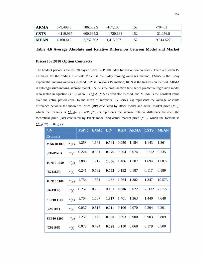
157
ARMA 679,499.3 786,602.5 -107,103 152 -704.63
CSTS -4,119,967 600,665.3 -4,720,633 152 -31,056.8
MEAN 4,168,410 2,752,602 1,415,807 152 9,314.522
Table 4.6 Average Absolute and Relative Differences between Model and Market
Prices for 2010 Option Contracts
The holdout period is the last 20 days of each S&P 500 index futures option contracts. There are seven IV
estimates for the trading rule test: MAV5 is the 5-day moving averages method, EMA5 is the 5-day
exponential moving averages method, LIV is Previous IV method, RGN is the Regression method, ARMA
is autoregressive-moving-average model, CSTS is the cross-section time series predictive regression model
represented in equation (4.16) where using ARMA as predictor method, and MEAN is the constant value
over the entire period equal to the mean of individual IV series. (a) represents the average absolute
difference between the theoretical price (BP) calculated by Black model and actual market price (MP),
which the formula is ∑ |𝐵𝑃𝑖 −𝑀𝑃𝑖|𝑘𝑖=1 /𝑘. (r) represents the average relative difference between the
theoretical price (BP) calculated by Black model and actual market price (MP), which the formula is
∑ (𝐵𝑃𝑖 −𝑀𝑃𝑖)𝑘𝑖=1 /𝑘.
*IV
Estimate
MAV5 EMA5 LIV RGN ARMA CSTS MEAN
MAR10 1075
(C070WC)
*(a) 1.253 1.161 0.944 0.950 1.154 1.143 1.861
*(r) 0.224 0.561 0.076 0.204 0.074 -0.212 0.235
JUN10 1050
(B243UE)
*(a) 1.880 1.717 1.356 1.406 1.707 1.694 11.077
*(r) 0.241 0.782 0.092 0.192 0.187 0.117 0.189
JUN10 1100
(B243UF)
*(a) 1.754 1.581 1.237 1.264 1.382 1.347 10.573
*(r) 0.257 0.752 0.101 0.006 0.022 -0.132 -0.355
SEP10 1100
(C9210T)
*(a) 1.704 1.587 1.317 1.401 1.363 1.440 4.648
*(r) 0.037 0.515 0.011 0.106 0.070 0.294 0.301
SEP10 1200
(C9210U)
*(a) 1.250 1.126 0.880 0.893 0.900 0.903 3.809
*(r) 0.078 0.424 0.028 0.130 0.068 0.179 0.500
158
Table 4.7 Average-Absolute and Relative Differences between Model and Market
Prices for 2011 Option Contracts
The holdout period is the last 20 days of each S&P 500 index futures option contracts. There are seven IV
estimates for the trading rule test: MAV5 is the 5-day moving averages method, EMA5 is the 5-day
exponential moving averages method, LIV is Previous IV method, RGN is the Regression method, ARMA
is autoregressive-moving-average model, CSTS is the cross-section time series predictive regression model
represented in equation (4.16) where using ARMA as predictor method, and MEAN is the constant value
over the entire period equal to the mean of individual IV series. (a) represents the average absolute
difference between the theoretical price (BP) calculated by Black model and actual market price (MP),
which the formula is ∑ |𝐵𝑃𝑖 −𝑀𝑃𝑖|𝑘𝑖=1 /𝑘. (r) represents the average relative difference between the
theoretical price (BP) calculated by Black model and actual market price (MP), which the formula is
∑ (𝐵𝑃𝑖 −𝑀𝑃𝑖)𝑘𝑖=1 /𝑘.
*IV
Estimate
MAV5 EMA5 LIV RGN ARMA CSTS MEAN
MAR11 1200
(D039NR)
*(a) 1.800 2.023 1.276 1.478 2.018 1.994 5.234
*(r) -0.041 1.353 -0.006 0.510 0.263 -0.166 2.735
MAR11 1250
(D1843V)
*(a) 1.619 1.670 1.136 1.496 1.461 1.438 4.445
*(r) 0.075 1.056 0.037 0.138 0.122 0.002 0.892
MAR11 1300
(D039NT)
*(a) 1.332 1.492 0.929 1.125 1.090 1.119 4.087
*(r) 0.041 1.005 0.017 0.025 0.065 0.049 0.068
JUN11 1325
(B513XF)
*(a) 1.274 1.448 0.927 1.089 1.096 1.100 2.515
*(r) 0.193 1.009 0.070 -0.075 0.027 -0.007 -0.363
JUN11 1350
(A850CJ)
*(a) 1.052 1.184 0.753 0.773 0.846 0.881 2.705
*(r) 0.188 0.893 0.064 0.075 0.091 0.149 0.060
SEP11 1250
(B9370T)
*(a) 1.595 1.769 1.192 1.235 1.274 1.536 4.160
*(r) -0.081 1.135 0.000 0.258 0.239 0.547 2.726
SEP11 1300
(B778PK)
*(a) 1.435 1.656 1.016 1.061 1.218 1.166 2.959
*(r) 0.056 1.205 0.038 0.318 0.228 0.087 2.086
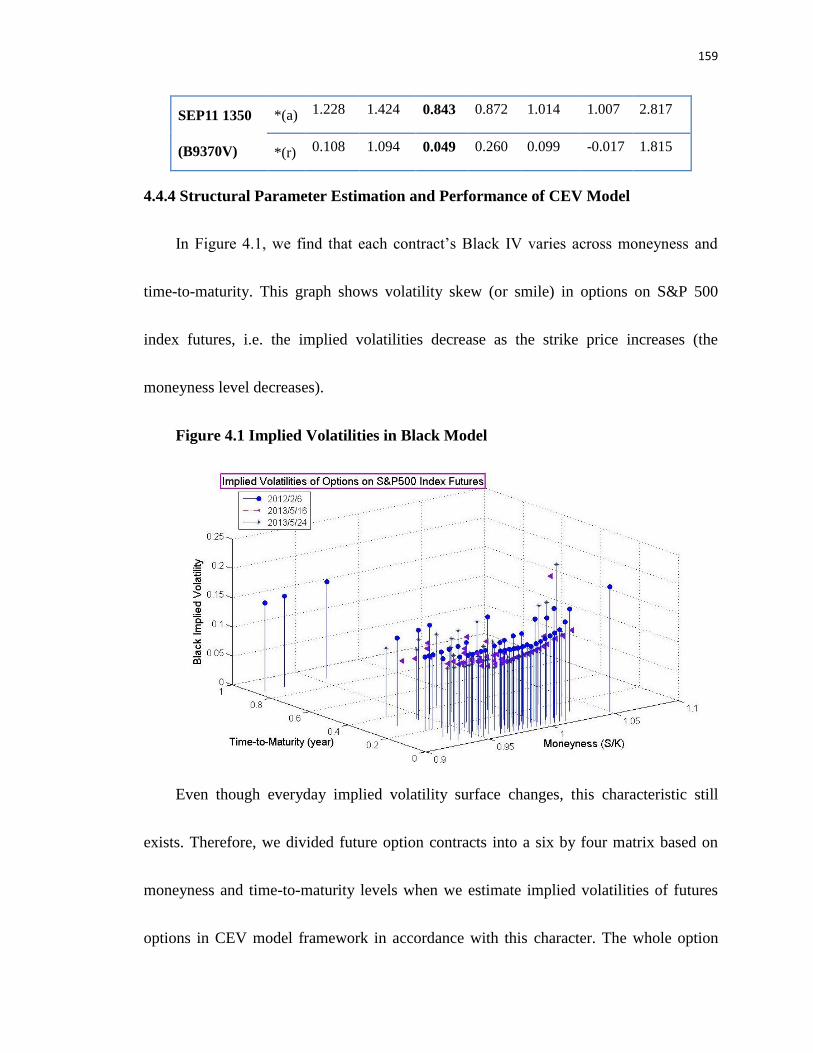
159
SEP11 1350
(B9370V)
*(a) 1.228 1.424 0.843 0.872 1.014 1.007 2.817
*(r) 0.108 1.094 0.049 0.260 0.099 -0.017 1.815
4.4.4 Structural Parameter Estimation and Performance of CEV Model
In Figure 4.1, we find that each contract’s Black IV varies across moneyness and
time-to-maturity. This graph shows volatility skew (or smile) in options on S&P 500
index futures, i.e. the implied volatilities decrease as the strike price increases (the
moneyness level decreases).
Figure 4.1 Implied Volatilities in Black Model
Even though everyday implied volatility surface changes, this characteristic still
exists. Therefore, we divided future option contracts into a six by four matrix based on
moneyness and time-to-maturity levels when we estimate implied volatilities of futures
options in CEV model framework in accordance with this character. The whole option
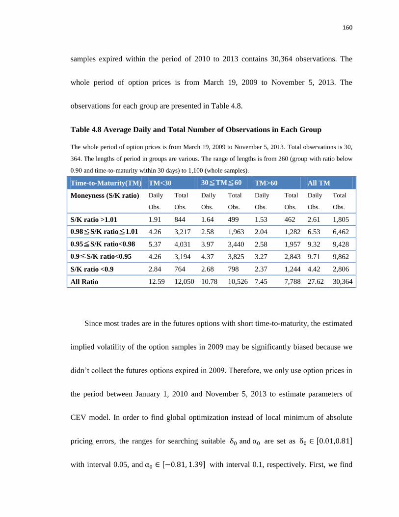
160
samples expired within the period of 2010 to 2013 contains 30,364 observations. The
whole period of option prices is from March 19, 2009 to November 5, 2013. The
observations for each group are presented in Table 4.8.
Table 4.8 Average Daily and Total Number of Observations in Each Group
The whole period of option prices is from March 19, 2009 to November 5, 2013. Total observations is 30,
364. The lengths of period in groups are various. The range of lengths is from 260 (group with ratio below
0.90 and time-to-maturity within 30 days) to 1,100 (whole samples).
Time-to-Maturity(TM) TM<30 30≦TM≦60 TM>60 All TM
Moneyness (S/K ratio) Daily
Obs.
Total
Obs.
Daily
Obs.
Total
Obs.
Daily
Obs.
Total
Obs.
Daily
Obs.
Total
Obs.
S/K ratio >1.01 1.91 844 1.64 499 1.53 462 2.61 1,805
0.98≦S/K ratio≦1.01 4.26 3,217 2.58 1,963 2.04 1,282 6.53 6,462
0.95≦S/K ratio<0.98 5.37 4,031 3.97 3,440 2.58 1,957 9.32 9,428
0.9≦S/K ratio<0.95 4.26 3,194 4.37 3,825 3.27 2,843 9.71 9,862
S/K ratio <0.9 2.84 764 2.68 798 2.37 1,244 4.42 2,806
All Ratio 12.59 12,050 10.78 10,526 7.45 7,788 27.62 30,364
Since most trades are in the futures options with short time-to-maturity, the estimated
implied volatility of the option samples in 2009 may be significantly biased because we
didn’t collect the futures options expired in 2009. Therefore, we only use option prices in
the period between January 1, 2010 and November 5, 2013 to estimate parameters of
CEV model. In order to find global optimization instead of local minimum of absolute
pricing errors, the ranges for searching suitable δ0 and α0 are set as δ0 ∈ [0.01,0.81]
with interval 0.05, and α0 ∈ [−0.81, 1.39] with interval 0.1, respectively. First, we find
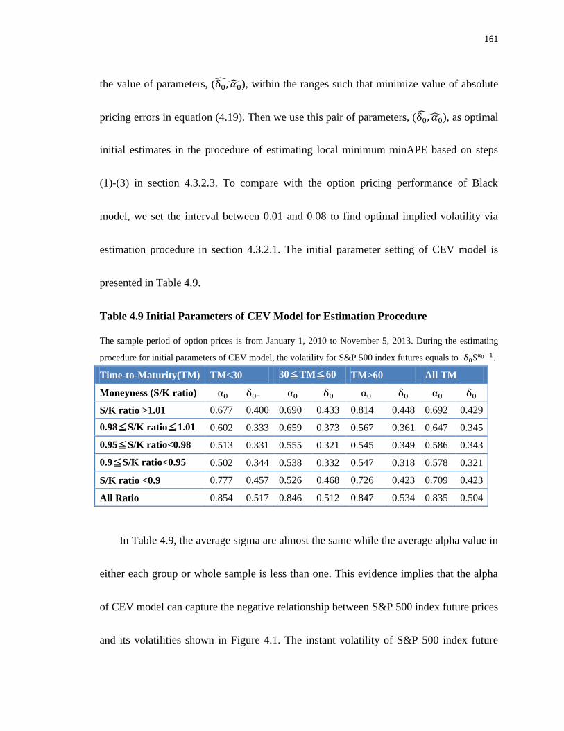
161
the value of parameters, (δ0̂, 𝛼0̂), within the ranges such that minimize value of absolute
pricing errors in equation (4.19). Then we use this pair of parameters, (δ0̂, 𝛼0̂), as optimal
initial estimates in the procedure of estimating local minimum minAPE based on steps
(1)-(3) in section 4.3.2.3. To compare with the option pricing performance of Black
model, we set the interval between 0.01 and 0.08 to find optimal implied volatility via
estimation procedure in section 4.3.2.1. The initial parameter setting of CEV model is
presented in Table 4.9.
Table 4.9 Initial Parameters of CEV Model for Estimation Procedure
The sample period of option prices is from January 1, 2010 to November 5, 2013. During the estimating
procedure for initial parameters of CEV model, the volatility for S&P 500 index futures equals to δ0Sα0−1.
Time-to-Maturity(TM) TM<30 30≦TM≦60 TM>60 All TM
Moneyness (S/K ratio) α0 δ0. α0 δ0 α0 δ0 α0 δ0
S/K ratio >1.01 0.677 0.400 0.690 0.433 0.814 0.448 0.692 0.429
0.98≦S/K ratio≦1.01 0.602 0.333 0.659 0.373 0.567 0.361 0.647 0.345
0.95≦S/K ratio<0.98 0.513 0.331 0.555 0.321 0.545 0.349 0.586 0.343
0.9≦S/K ratio<0.95 0.502 0.344 0.538 0.332 0.547 0.318 0.578 0.321
S/K ratio <0.9 0.777 0.457 0.526 0.468 0.726 0.423 0.709 0.423
All Ratio 0.854 0.517 0.846 0.512 0.847 0.534 0.835 0.504
In Table 4.9, the average sigma are almost the same while the average alpha value in
either each group or whole sample is less than one. This evidence implies that the alpha
of CEV model can capture the negative relationship between S&P 500 index future prices
and its volatilities shown in Figure 4.1. The instant volatility of S&P 500 index future

162
prices equals to δ0Sα0−1 where S is S&P 500 index future prices, δ0 and α0 are the
parameters in CEV model. The estimated parameters in Table 4.9 are similar across
time-to-maturity level but volatile across moneyness.
Because of the implementation and computational costs, we select the sub-period
from January 2012 to November 2013 to analyze the performance of CEV model. The
total number of observations and the length of trading days in each group are presented in
Table 4.10. The estimated parameters in Table 4.9 are similar across time-to-maturity
level but volatile across moneyness. Therefore, we investigate the performance of all
groups except the groups on the bottom row of Table 4.10. The performance of models
can be measured by either the implied volatility graph or the average absolute pricing
errors (AveAPE). The implied volatility graph should be flat across different moneyness
level and time-to-maturity. We use subsample like Bakshi et al. (1997) and Chen et al.
(2009) did to test implied volatility consistency among moneyness-maturity categories.
Using the subsample data from January 2012 to May 2013 to test in-the-sample fitness,
the average daily implied volatility of both CEV and Black models, and average alpha of
CEV model are computed in Table 4.11. The fitness performance is shown in Table 4.12.
The implied volatility graphs for both models are shown in Figure 4.2. In Table 4.11, we
estimate the optimal parameters of CEV model by using a more efficient program. In this
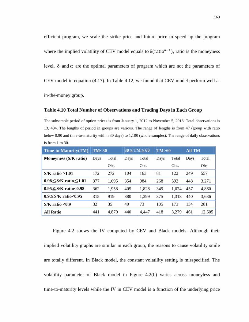
163
efficient program, we scale the strike price and future price to speed up the program
where the implied volatility of CEV model equals to δ(ratioα−1), ratio is the moneyness
level, δ and α are the optimal parameters of program which are not the parameters of
CEV model in equation (4.17). In Table 4.12, we found that CEV model perform well at
in-the-money group.
Table 4.10 Total Number of Observations and Trading Days in Each Group
The subsample period of option prices is from January 1, 2012 to November 5, 2013. Total observations is
13, 434. The lengths of period in groups are various. The range of lengths is from 47 (group with ratio
below 0.90 and time-to-maturity within 30 days) to 1,100 (whole samples). The range of daily observations
is from 1 to 30.
Time-to-Maturity(TM) TM<30 30≦TM≦60 TM>60 All TM
Moneyness (S/K ratio) Days Total
Obs.
Days Total
Obs.
Days Total
Obs.
Days Total
Obs.
S/K ratio >1.01 172 272 104 163 81 122 249 557
0.98≦S/K ratio≦1.01 377 1,695 354 984 268 592 448 3,271
0.95≦S/K ratio<0.98 362 1,958 405 1,828 349 1,074 457 4,860
0.9≦S/K ratio<0.95 315 919 380 1,399 375 1,318 440 3,636
S/K ratio <0.9 32 35 40 73 105 173 134 281
All Ratio 441 4,879 440 4,447 418 3,279 461 12,605
Figure 4.2 shows the IV computed by CEV and Black models. Although their
implied volatility graphs are similar in each group, the reasons to cause volatility smile
are totally different. In Black model, the constant volatility setting is misspecified. The
volatility parameter of Black model in Figure 4.2(b) varies across moneyless and
time-to-maturity levels while the IV in CEV model is a function of the underlying price

164
and the elasticity of variance (alpha parameter). Therefore, we can image that the
prediction power of CEV model will be better than Black model because of the explicit
function of IV in CEV model. We can use alpha to measure the sensitivity of relationship
between option price and its underlying asset. For example, in Figure 4.2(c), the
in-the-money future options near expired date have significantly negative relationship
between future price and its volatility.
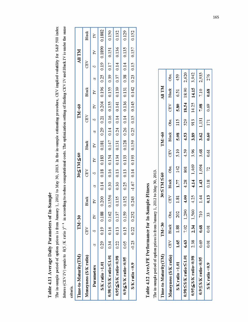
165
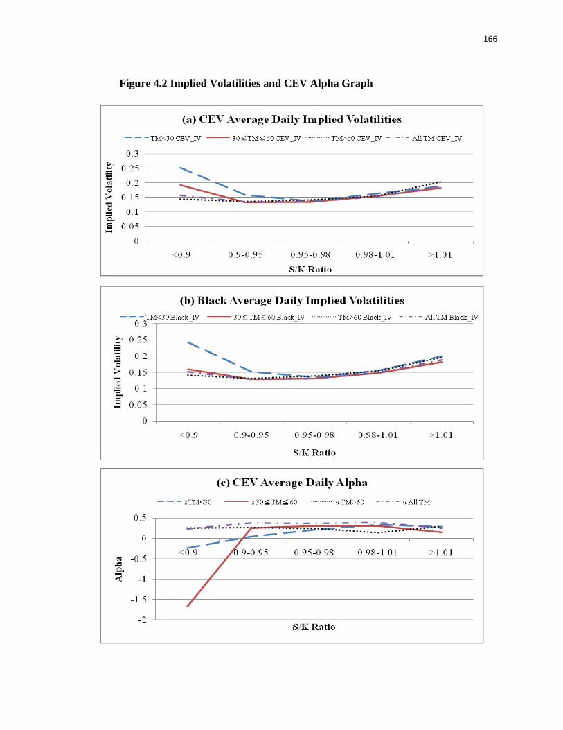
166
Figure 4.2 Implied Volatilities and CEV Alpha Graph
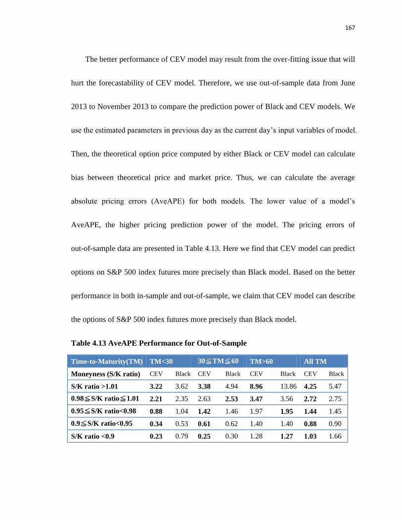
167
The better performance of CEV model may result from the over-fitting issue that will
hurt the forecastability of CEV model. Therefore, we use out-of-sample data from June
2013 to November 2013 to compare the prediction power of Black and CEV models. We
use the estimated parameters in previous day as the current day’s input variables of model.
Then, the theoretical option price computed by either Black or CEV model can calculate
bias between theoretical price and market price. Thus, we can calculate the average
absolute pricing errors (AveAPE) for both models. The lower value of a model’s
AveAPE, the higher pricing prediction power of the model. The pricing errors of
out-of-sample data are presented in Table 4.13. Here we find that CEV model can predict
options on S&P 500 index futures more precisely than Black model. Based on the better
performance in both in-sample and out-of-sample, we claim that CEV model can describe
the options of S&P 500 index futures more precisely than Black model.
Table 4.13 AveAPE Performance for Out-of-Sample
Time-to-Maturity(TM) TM<30 30≦TM≦60 TM>60 All TM
Moneyness (S/K ratio) CEV Black CEV Black CEV Black CEV Black
S/K ratio >1.01 3.22 3.62 3.38 4.94 8.96 13.86 4.25 5.47
0.98≦S/K ratio≦1.01 2.21 2.35 2.63 2.53 3.47 3.56 2.72 2.75
0.95≦S/K ratio<0.98 0.88 1.04 1.42 1.46 1.97 1.95 1.44 1.45
0.9≦S/K ratio<0.95 0.34 0.53 0.61 0.62 1.40 1.40 0.88 0.90
S/K ratio <0.9 0.23 0.79 0.25 0.30 1.28 1.27 1.03 1.66

168
4.5 Conclusion
For the academician, the inconsistent cross-sectional and time series nature of the IV
implies a certain and perhaps significant degree of misspecification within BSM /Black
option pricing model.
The purpose of this essay has been to improve the interpretation and forecasting of
individual implied volatility (IV) for call options on S&P500 index futures in 2010 to
2013. The two alternative methods used in this essay are cross-sectional time-series
analysis and CEV model. These two alternative approaches give different perspective of
estimating IV. The cross-sectional time series analysis focuses on the dynamic behavior
of volatility in each option contracts and captures other trading behaviors such as week
effect and in/out of the money effect. On the other hand, CEV model generalizes implied
volatility surface as a function of asset price.
By empirically explaining the composition through time series analysis and
cross-sectional time series regression models, the disadvantages to evaluating an option
IV by Black model have been demonstrated. More importantly, the results based on our
trading strategy provide some evidence as to how the Black option pricing model might
be misspecified, or jointly, how the market might be inefficient. Though the original
169
model implicitly assumes a frictionless market and a constant volatility term, market
realities along with past studies would not be able to substantiate these types of
assumptions. The forecasting performances of seven time-series regression models based
on our trading strategy show that the simple regression models perform better than
sophisticated cross-sectional time-series models because of over-fitting problem in the
advanced models. In addition, although our trading rules based on the prediction of these
models can make profit, the net profit depends on the transaction costs. Therefore, the
setting of trading strategy should be necessarily adjusted to the transaction costs.
We also show that CEV model performs better than Black model in aspects of either
in-sample fitness or out-of-sample prediction. The setting of CEV model is more
reasonable to depict the negative relationship between S&P 500 index future price and its
volatilities. The elasticity of variance parameter in CEV model captures the level of this
characteristic. The stable volatility parameter in CEV model in our empirical results
implies that the instantaneous volatility of index future is mainly determined by current
future price and the level of elasticity of variance parameter.
In sum, we suggest predict individual option contract by using simple regression
analysis instead of advanced cross-sectional time-series model. Even though the
moneyness and week effect have significant influence on index future option prices, the

170
over-fitting problem in an advanced cross-sectional time-series model will decrease its
pricing forecastability. With regard to generate implied volatility surface to capture whole
prediction of the future option market, the CEV model is the better choice than Black
model because it not only captures the skewness and kurtosis effects of options on index
futures but also has less computational costs than other jump-diffusion stochastic
volatility models.
171
CHAPTER 5
Summary and Future Study
This thesis includes three essays in chapters 2 to 4 respectively related to capital
structure, risk management in banking, and options on index futures. The first essay in
chapter 2 investigates the determinants of capital structure and the joint determination of
capital structure and stock rate of return by using structure equation modeling (SEM)
approach. The second essay in chapter 3 proposes the structural model approach in terms
of the Stair Tree model and the barrier option model to price fair deposit insurance
premium in accordance with closure policy, bankrupt costs, and practical provisions and
restrictions of insurance contracts. Finally, the purpose of the third essay is to improve the
interpretation and forecasting of individual implied volatility for call options on S&P500
index futures by using cross-sectional time series regression and CEV models. The
results of these three essays are as following.
In chapter 2, we utilize the structure equation modeling (SEM) with CFA approach
estimate the impacts of unobservable attributes on capital structure. The main
contribution of this essay is the comprehensive confirmation on theories in corporate
finance. Based on the sample during 2001 to 2012, our empirical work only shows

172
“Profitability” and “Volatility & Financial Rating” are significant attributes on the
decision of capital structure. However, all attributes become significant determinants of
capital structure and stock returns in either market- or book- value basis. The evidence
shows that the interaction of a firm’s leverage and its stock price should be necessarily
considered in capital structure research. Besides the proof of trade-off between financial
distress and agency costs in previous theories, our results confirm the endogenous supply
relationship between public and private debts. Moreover, the interrelation between
leverage ratios and stock returns verifies the signal theory under the assumption of
asymmetric information between managers and investors. Only significantly negative
influence of stock returns on market-value based leverage ratios supports Welch’s (2004)
statement. We also do robustness check by using MIMIC model and the two-stage, least
square (2SLS) estimating method. However, MIMIC model and 2SLS method cannot
well identify the influences of factors on long-term leverage decisions in accordance with
capital structure theories. According to comparison of these methods’ results, the setting
of latent attributes is necessary to clarify and confirm theories in capital structure.
Therefore, I would suggest using structural equation modeling (SEM) with confirmatory
factor analysis (CFA) to capture the appropriate factors of firms’ leverage decisions.
The simulation results in chapter 3 first indicate that our structural model approach

173
is the general model to evaluate deposit insurance and the model in Brockman and Turle
(2003) (hereafter called BT) is a special case of mine. Moreover, the interaction between
closure policy and bankruptcy is incorporated in our model and the results manifest the
important role of bankrupt costs in FDIC supervision. Even though the increase in
regulatory barrier will lead to transfer the wealth from stockholders to the insurer, the
indirectly bankrupt costs will offset this benefit. Therefore, FDIC would prefer to take the
forbearance closure policy rather than the strict policy to protect insurance fund from loss
of bankrupt costs. The closure policy can be properly adjusted by the setting of insurance
premium and the impacts of bankruptcy cost. Finally, an appropriate deposit insurance
premium can alleviate potential moral hazard problems caused by a forbearance policy.
The empirical results of chapter 4 by using options on S&P 500 index futures
expired in 2010 to 2013 shows that implied volatility is predictable. The two alternative
approaches, cross-sectional time-series analysis and CEV model, give different
perspective of estimating IV in the third essay. The cross-sectional time series analysis
focuses on the dynamic behavior of volatility in each option contracts and captures other
trading behaviors such as week effect and in/out of the money effect. On the other hand,
CEV model generalizes implied volatility surface as a function of asset price. The
abnormal returns in our trading strategy with transaction costs provide some evidence as
174
to how the Black option pricing model might be misspecified, or jointly, how the market
might be inefficient. According to the performance in terms of in-sample fitness and
out-of-sample prediction, CEV model is a better option pricing model than Black model.
It not only captures the skewness and kurtosis effects of options on index futures but also
has less computational costs than other jump-diffusion stochastic volatility models. In
addition, the setting of CEV model is more reasonable to depict the negative relationship
between S&P 500 index future price and its volatilities. The stable volatility parameter in
CEV model in our empirical results implies that the instantaneous volatility of index
future is mainly determined by current future price and the level of elasticity of variance
parameter. In sum, we suggest predict individual option contract by using time-series
analysis and generate implied volatility surface by using CEV model.
In future research, personal taxes and heterogeneous beliefs between manager and
outside investors can be taken into joint determinants of capital structure and stock return
if the related information is available. In second essay, if we can obtain real data to find
the fair deposit insurance premium and proper closure barrier, then we can confirm our
supposition that the forbearance policy is better than restrict policy for FDIC. Finally, we
can apply CEV model and its Greek measures to other liquid option markets to test
market efficiency based on our trading rules.
175
REFERENCE
Akaike, H. 1969. “Fitting autoregressive models for prediction.” Annals of the Institute of
Statistical Mathematics 21, 243-247.
Akaike, H. 1977. “On entropy maximization principle.” in Applications of Statistics, Ed.
P. R. Krishnaiah, Amsterdam, North Holland, 27-41.
Allen, L. and A. Saunders. 1993. “Forbearance and valuation of deposit insurance as a
callable put.” Journal of Banking and Finance 17, 629–643.
Altman, E. I. 1984. “A further empirical investigation of the bankruptcy cost question.”
Journal of Finance 39, 1067-1089.
Anderson, R., and S. Sundaresan. 2000. “A comparative study of structural models of
corporate bond yields: An exploratory investigation.” Journal of Banking and
Finance 24, 255-269.
Ansley, C. F. and P. Newbold. 1980. “Finite sample properties of estimators for
autoregressive moving average models.” Journal of Econometrics 13, 159-183.
Avery, R. B., G. A. Hanweck and M. L. Kwast. 1985. “An analysis of risk-based deposit
insurance for commercial banks.” Bank Structure and Competition, 217-250.
Bakshi, G, C Cao and Z Chen. 1997. “Empirical performance of alternative option
pricing models.” Journal of Finance, 52, 2003–2049.
Bakshi, G, C Cao and Z Chen. 2000. “Pricing and hedging long-term options.” Journal of
Econometrics, 94, 277–318.
Bakshi, G, C Cao, and Z Chen. 2009. “Option pricing and hedging performance under
stochastic volatility and stochastic interest rates.” In Handbook of Quantitative
Finance and Risk Management, C-F Lee, AC Lee, J Lee (eds.), 2010. New York:
Springer Science and Business.
Baker, M. P. and J. Wurgler. 2002. “Market timing and capital structure.” Journal of
Finance 57, 1–32.
176
Bansal, R., W.J. Coleman and C.T. Lundblad. 2011. “Endogenous liquidity supply.”
Working paper.
Beckers, S. 1980. “The constant elasticity of variance model and its implications for
option pricing.” Journal of Finance, 35, 661–673.
Benton, D. and K. Krishnamoorthy. 2003. “Compute discrete mixtures of continuous
distributions: Noncentral chisquare, noncentral t and the distribution of the square of
the sample multiple correlation coefficient.” Computational Statistics and Data
Analysis, 43, 249-267.
Berger, P. G., E. Ofek, and D. L. Yermack. 1997. “Managerial entrenchment and capital
structure decisions.” Journal of Finance 52, 1411-1438.
Bevan, A. A. and J. Danbolt. 2002. “Capital structure and its determinants in the UK—a
decompositional analysis.” Applied Financial Economics 12, 159-170.
Bhagat, S., B. Bolton, and A. Subramanian. 2011. “Manager characteristics and capital
structure: theory and evidence.” Journal of Financial and Quantitative Analysis 46,
1581-1627.
Black, F. and J. Cox. 1976. “Valuing corporate securities: some effects of bond indenture
provisions.” Journal of Finance 31,351-367.
Black, F. and M. Scholes. 1973. “The pricing of options and corporate liabilities.”
Journal of Political Economy 81, 637-659.
Black, F. 1975. “Fact and fantasy in the use of options.” Financial Analysts Journal 31,
36-41& 61-72.
Black, F. 1976. “The pricing of commodity contracts.” Journal of Financial Economics 3,
167-179.
Bloecher, E. P., G. A. Seals, and R. D. Vilim. 2003. “Options for pricing Federal deposit
insurance.” FDIC Banking Review 15, no. 4.
Bowen, R. M., L. A. Daley, and C. C. Huber, Jr. 1982. “Evidence on the existence and
determinants of inter-industry differences in leverage.” Financial Management 4,
177
10-20.
Box, G. E. P. and G. M. Jenkins. 1970. Time Series Analysis Forecasting and Control.
San Francisco: Holden-Day.
Brenner M. and D. Galai. 1981. “The properties of the estimated risk of common stocks
implied by option prices.” Working paper, University of California at Berkeley.
Brenner, M., G. Courtadon, and M. Subrahmanyam. 1985. “Options on the spot and
options on futures.” Journal of Finance 40, 1303-1317.
Brockman, P. and H.J. Turtle. 2003. “A barrier option framework for corporate security
valuation.” Journal of Financial Economics 67, 511-529.
Burdett, K. 1978. “A theory of employee job search and quit rates.” American Economic
Review 68, 212-220.
Chance, D. M. 1986. “Empirical tests of the pricing of index call options.” Advances in
Futures and Options Research 1, 141-166.
Chang, C., A. Lee, and C. F. Lee. 2009. “Determinants of capital structure choice: a
structural equation modeling approach.” The Quarterly Review of Economic and
Finance 49, 197-213.
Chen, R and C.F. Lee. 1993. “A constant elasticity of variance family of stock prices in
option pricing: Review and integration.” Journal of Financial Studies, 1, 29–51.
Chen, R., C.F. Lee. and H. Lee. 2009. “Empirical performance of the constant elasticity
variance option pricing model.” Review of Pacific Basin Financial Markets and
Policies, 12(2), 177–217.
Chevalier, J. 1995. “Do LBO supermarkets charge more? An empirical analysis of the
effects of LBOs on supermarket pricing.” Journal of Finance 50, 1095–1112.
Chiras, D. and S. Manaster. 1978. “The information content of option prices and a test of
market efficiency.” Journal of Financial Economics 6, 213-234.
Cox, J. C. 1975. “Notes on option pricing I: constant elasticity of variance diffusions.”
178
Working paper, Stanford University.
Cox, J. C. and S. A. Ross. 1976. “The valuation of options for alternative stochastic
processes.” Journal of Financial Economics 3, 145-166.
Dai, T.-S. 2009. “Efficient option pricing on stocks paying discrete or path-dependent
dividends with the stair tree.” Quantitative Finance 9, 827-838.
Day, T.E. and C. M. Lewis. 1992. “Stock market volatility and the information content of
stock index options.” Journal of Econometrics, 52, 267-287.
DeAngelo, H. and R. Masulis. 1980. “Optimal capital structure under corporate and
personal taxation.” Journal of Financial Economics 8, 3-27.
DelBaen, F and H Sirakawa. 2002. A note on option pricing for the constant elasticity of
variance model. Asia-Pacific Financial Markets, 9, 85–99.
Diamond, D., and P. Dybvig. 1983. “Bank runs, deposit insurance, and liquidity.” Journal
of Political Economy 91,401-419.
Ding, C.G. 1992. “Algorithm AS275: Computing the non-central χ2 distribution
function.” Applied Statistics, 41, 478-482.
Dittmar, A., and A. Thakor. 2007. “Why do firms issue equity?” Journal of Finance 62,
1-54.
Duffie, D., R. Jarrow, A. Purnanandam, and W. Yang. 2003. “Market pricing of deposit
insurance.” Journal of Financial Services Research 24, 93-119.
Dumas, B., J. Fleming and R. E. Whaley. 1998. Implied volatility functions: empirical
tests. Journal of Finance, 53, 2059-2106.
Emanuel, DC and JD MacBeth. 1982. “Further results on the constant elasticity of
variance call option pricing model.” Journal of Financial and Quantitative Analysis,
17, 533–554.
Engle, R. F. 1982.” Autoregressive conditional heteroskedasticity with estimates of the
variance of U.K. inflation.” Econometrica, 50, 987-1008.
179
Episcopos, A. 2008. “Bank capital regulation in a barrier option framework.” Journal of
Banking and Finance 32, 1677-1686.
Falkenheim, M., and G. Pennacchi. 2003. “The cost of deposit insurance for privately
held banks: A market comparable approach.” Journal of Financial Services Research
24, 121-148.
Fama, E. F. and K. R. French. 2002. “Testing tradeoff and pecking order predictions
about dividends and debt.” Review of Financial Studies 15, 1-33.
FDIC. 2006. “Rules and regulations.” Federal Register 71, no. 230.
Fischer, E., R. Heinkel, and J. Zechner. 1989. “Dynamic capital structure choice: theory
and tests.” Journal of Finance 44, 19-40.
Fleming, J. 1998. “The quality of market volatility forecasts implied by S&P 100 index
option prices.” Journal of Empirical Finance, 5, 317-345.
Fleming, J., B. Ostdiek, and R. E. Whaley. 1996. “Trading costs and the relative rates of
price discovery in stock, futures, and option markets.” Journal of Futures Markets,
16, 353-387.
Frank, M. and V. Goyal. 2009. “Capital structure decisions: Which factors are reliably
important?” Financial Management 38, 1-37.
Gan, L. and G. W. Y. Wang. 2013. “Partial deposit insurance and moral hazard in
banking.” International Journal of Commerce and Management, 23, 8-23.
Geske, R. 1979. “The valuation of compound options.” Journal of Financial Economics 7,
63-81.
Geske, R. and R. Roll. 1984. “On valuing American call options with Black-Scholes
European formula.” Journal of Finance 39, 443-455.
Graham, J. 2000. “How big are the tax benefits of debt?” Journal of Finance 55,
1901-1941.
Graham, J. R., M. T. Leary, and M. R. Roberts. 2012. A century of capital structure: The
180
leveraging of corporate America. Working paper.
Greenwood, R., S. Hanson, and J. C. Stein. 2010. “A Gap-Filling Theory of Corporate
Debt Maturity Choice." Journal of Finance 65, 993-1028.
Greenwood, R., and D. Vayanos. 2010. “Price pressure in the government bond market.”
American Economic Review 100, 585‐590.
Greenwood, R., and D. Vayanos. 2008. “Bond Supply and Excess Bond Returns.”
Working paper.
Gorton, G., and G. Pennacchi. 1990. “Financial intermediaries and liquidity creation.”
Journal of Finance 45, 49-71.
Grossman, S. and O. Hart. 1982. “Corporate financial structure and managerial
incentives.” The Economics of Information and Uncertainty, Chicago: University of
Chicago Press.
Hannan, E. J. and J. Rissanen. 1982. “Recursive estimation of mixed
autoregressive-moving average order.” Biometrika 69, 81-94.
Harvey, C. R. and R. E. Whaley. 1991. “S&P 100 index option volatility.” Journal of
Finance, 46, 1551-1561.
Harvey, C. R. and R. E. Whaley. 1992a. “Market volatility prediction and the efficiency
of the S&P 100 index option market.” Journal of Financial Economics, 31, 43-73.
Harvey, C. R. and R. E. Whaley. 1992b. “Dividends and S&P 100 index option valuation.”
Journal of Futures Market, 12, 123-137.
Heston, SL. 1993. “A closed-form solution for options with stochastic volatility with
applications to bond and currency options.” Review of Financial Studies, 6, 327–343.
Hillmer, S. C. and G. C. Tiao. 1979. “Likelihood function of stationary multiple
autoregressive moving average models.” Journal of the American Statistical
Association 74, 652-660.
Hsu, Y.L., T.I. Lin, and C.F. Lee. 2008. “Constant elasticity of variance (CEV) option
181
pricing model: Integration and detailed derivation.” Mathematics and Computers in
Simulation, 79, 60-71.
Hull, J. C. 2011. Options, Futures, and Other Derivatives, 8th edition. Englewood Cliffs,
NJ: Prentice-Hall.
Hull, JC and A White. 1987. “The pricing of options on assets with stochastic volatility.”
Journal of Finance, 42, 281–300.
Horvitz, P. 1983. “The case against risk-adjusted deposit insurance premiums.”
Housing Finance Review 2, 253-264.
Hwang, D.-Y., C. F. Lee and T. K. Liaw. 1997. “Forecasting bank failures and deposit
insurance premium.” International Review of Economics and Finance 6, 317-334.
Hwang, D.-Y., F.-S. Shie, K. Wang and J.-C. Lin. 2009. “The pricing of deposit insurance
considering bankruptcy costs and closure policies.” Journal of Banking and Finance
33, 1909-1919.
Jackwerth, JC and M Rubinstein. 2001. “Recovering stochastic processes from option
prices.” Working paper, London Business School.
Jarrow R. and A. Rudd. 1982. “Approximate option valuation for arbitrary stochastic
processes.” Journal of Financial Economics 10, 347-369.
Jarrow, R. and A. Rudd. 1983. “Tests of an approximate option valuation formula.” in
Option Pricing: Theory and Applications, Ed. M. Brenner, Lexington, MA:
Lexington Books, 81-100.
Jensen, M. 1986. “Agency costs of free cash flow, corporate financing, and takeovers.”
American Economic Review 76, 323–329.
Jensen, M. C. and W. H. Meckling. 1976. “Theory of the firm: managerial behavior,
agency costs and ownership structure.” Journal of Financial Economics 3, 305-360.
Jenter, D. 2005. “Market timing and managerial portfolio decisions.” Journal of Finance,
60, 1903-1949.
182
Jenter, D., K. Lewellen, and J.B. Warner. 2011. “Security issue timing: what do managers
know, and when do they know it?” Journal of Finance, 66, 413-443.
Jones, CS. 2003. “The dynamics of stochastic volatility: Evidence from underlying and
option markets.” Journal of Econometrics, 116, 181–224.
Joreskog, K. G. 1977. "Structural equation models in the social sciences: specification
estimation and testing." In P. R. Krishnaiah (ed.).
Joreskog, K. G. and D. Sorbom. 1981. "LISREL V, analysis of linear structural
relationships by the method of maximum likelihood." Chicago: National
Educational Resources.
Joreskog, K. G. and A. S. Goldberger. 1975. “Estimation of a model with multiple
indicators and multiple causes of a single latent variable.” Journal of American
Statistical Association 70, 631-639.
Joreskog, K. G. and D. Sorbom. 1989. “LISREL 7: A guide to the program and
applications, 2nd ed.” SPSS.
Jung, H. W. and A. Subramanian. 2010. “Capital structure under heterogeneous beliefs.”
Working paper.
Karas, A., W. Pyle, and K. Schoors. 2013. “Deposit insurance, banking crises, and market
discipline: evidence from a natural experiment on deposit flows and rates. “ Journal
of Money, Credit and Banking, 45(1), 179-200.
Kane, E. 1986. “Appearance and reality in deposit insurance: The case for reform.”
Journal of Banking and Finance 10, 175-188.
Krishnamurthy, A. and A. Vissing-Jorgensen. 2010. “The aggregate demand for Treasury
debt.” Working paper.
Laeven, L. 2002. “International evidence on the value of deposit insurance.” Quarterly
Review of Economics and Finance 42, 721-732.
Larguinho M., J.C. Dias, and C.A. Braumann. 2013. “On the computation of option
prices and Greeks under the CEV model.” Quantitative Finance, 13(6), 907-917.
183
Latane, H. A. and R. J. Rendleman. 1976. “Standard deviations of stock price ratios
implied in option prices.” Journal of Finance 31, 369-381.
Leary, M. and M. Roberts. 2005. “Do firms rebalance their capital structures?” Journal of
Finance 60, 2575–2620.
Lee, R. W. 2001. “Implied and local volatilities under stochastic volatility.” International
Journal of Theoretical and Applied Finance, 4, 45-89.
Lee, C. F. and C. Wu. 1985. “The impacts of kurtosis on risk stationarity: some empirical
evidence.” Financial Review 20, 263-269.
Lee, C.F., T. Wu and R. Chen. 2004. “The constant elasticity of variance models: New
evidence from S&P 500 index options.” Review of Pacific Basin Financial Markets
and Policies, 7(2), 173–190.
Lee, S. C., J. P. Lee, and M. T. Yu. 2005. “Bank capital forbearance and valuation of
deposit insurance.” Canadian Journal of Administrative Sciences 22, 220-229.
Leland, H. 1994. “Corporate debt value, bond covenants, and optimal capital structure.”
Journal of Finance 49, 1213-1252.
LeRoy, S. F. and R.Singhania. 2013. “Bank deposit insurance: implications for portfolios
and equilibrium valuation of risky assets.” Working paper.
Lewis, A. S. 2000. Option Valuation under stochastic volatility with Mathematica code,
NewportBeach, CA: Finance Press.
Lin, L. and M. J. Flannery. 2013. “Do personal taxes affect capital structure? Evidence
from the 2003 tax cut.” Journal of Financial Economics, 109(2), 549-565.
Maddala, G. S. and M. Nimalendran. 1996. “Error-in-variables problems in financial
models.” Handbook of Statistics 14, Elsevier Science Publishers B. V., 507-528.
Macbeth, J. D. and L. J. Merville. 1979. “An empirical examination of the Black-Scholes
call option pricing model.” Journal of Finance 34, 1173-1186.
MacBeth, JD and LJ Merville. 1980. “Tests of the Black-Scholes and Cox Call option
184
valuation models.” Journal of Finance, 35, 285–301.
MacKie-Mason, J. 1990. “Do taxes affect corporate financing decisions?” Journal of
Finance 45, 1471–1493.
Marcus, A. J. and I. Shaked. 1984. “The valuation of FDIC deposit insurance using
option-pricing estimates.” Journal of Money, Credit and Banking 16, 446-460.
Marsh, P. 1982. “The choice between equity and debt: An empirical study.” Journal of
Finance 37, 121–144.
Medvedev A. and O. Scaillet. 2007. “Approximation and calibration of short-term
implied volatilities under jump-diffusion stochastic volatility.” Review of Financial
Studies, 20, 427-459.
McDonald, R. 1983. “Government debt and private leverage: An extension of the Miller
theorem.” Journal of Public Economics 22, 303-325.
Merton, R. C. 1973. “Theory of rational option pricing.” Bell Journal of Economics and
Management science 4, 141-183.
Merton, R. C. 1976. “Option pricing when underlying stock returns are discontinuous.”
Journal of Financial Economics 3, 125-144.
Merton, R. C. 1977. “An analytic derivation of the cost of deposit insurance and loan
guarantees.” Journal of Banking and Finance 1, 3-11.
Merton, R. C. 1978. “On the cost of deposit insurance when there are surveillance costs.”
Journal of Business 51, 439–452.
Miller, M. 1977. “Debt and taxes” Journal of Finance 32, 261-275.
Myers, S. C. 1977. “Determinants of corporate borrowing.” Journal of Financial
Economics 5, 146-175.
Myers, S. C. and N. Majluf. 1984. “Corporate financing and investment decision when
firms have information investors do not have.” Journal of Financial Economics 13,
187-221.
185
O’Hara, M. 1983. “A dynamic theory of the banking firm.” Journal of Finance 38,
127-140.
Ramaswamy, K. and S. M. Sundaresan. 1985. “The valuation of options on futures
contracts.” Journal of Finance 40, 1319-1340.
Rampini, A. A. and S. Viswanathan. 2013. “Collateral and capital structure.” Journal of
Financial Economics, 109(2), 466-492.
Pagan, A.R. and G.W. Schwert. 1990. “Alternative models for conditional stock volatility.”
Journal of Econometrics, 45, 267-290.
Park, H. Y. and R. S. Sears. 1985. “Estimating stock index futures volatility through the
prices of their options.” Journal of Futures Markets 5, 223-237.
Parrino, R. and M. Weisbach. 1999. “Measuring investment distortions arising from
stockholder-bondholder conflicts.” Journal of Financial Economics 52, 3–42.
Pastor, L., Stambaugh R. 2003. “Liquidity risk and expected stock returns.” Journal of
Political Economy 111, 642-685.
Phillips, S.M. and C.W. Smith. 1980. Trading costs for listed options: The implications
for market efficiency. Journal of Financial Economics, 8, 179-201.
Phillips, G. 1995. “Increased debt and industry product markets: An empirical analysis.”
Journal of Financial Economics 37, 189–238.
Pun C. S. and H.Y. Wong. 2013. “CEV asymptotics of American options.” Journal of
Mathematical Analysis and Applications, 403(2), 451-463.
Rajan, R. G., and L. Zingales. 1995. “What do we know about capital structure? Some
evidence from international data.” Journal of Finance 50, 1421–1460.
Ronn, E. I. and A. K. Verma. 1986. “Pricing risk-adjusted deposit insurance: An
option-based model.” Journal of Finance 41, 871-895.
Rubenstein, M. 1985. “Nonparametric Tests of Alternative Option Pricing Models Using
All Reported Trades and Quotes on the 30 Most Active CBOE Option Classes from
186
August 23, 1976 through August 31, 1978.” Journal of Finance 40, 455-480.
Schroder, M. 1989. “Computing the constant elasticity of variance option pricing
formula.” Journal of Finance, 44(1), 211–219.
Schmalensee, R. and R. Trippi. 1978 . “Common stock volatility estimates implied by
option premia.” Journal of Finance 33, 129-147.
Schwarz, G. 1978. “Estimating the dimension of a model.” Annals of Statistics 6,
461-464.
Scott, LO. 1987. “Option pricing when the variance changes randomly: Theory,
estimation, and an application.” Journal of Financial and Quantitative Analysis, 22,
419–438.
Scott, LO. 1997. “Pricing stock options in a jump-diffusion model with stochastic
volatility and interest rate: Application of Fourier inversion methods.” Mathematical
Finance, 7(4), 413–424.
Singh, V.K. and N. Ahmad. 2011. “Forecasting performance of constant elasticity of
variance model: empirical evidence from India.” International Journal of Applied
Economics and Finance, 5, 87-96.
Sinkey, J. F. 1975. “A multivariate statistical analysis of the characteristics of problem
banks.” Journal of Finance 30, 21-36.
Stein, EM and JC Stein. 1991. “Stock price distribution with stochastic volatility: An
analytical approach.” Review of Financial Studies, 4, 727–752.
Stephan, J.A. and R.E. Whaley. 1990. “Intraday price change and trading volume
relations in the stock and stock option markets.” Journal of Finance, 45, 191-220.
Stulz, R. 1990. “Managerial discretion and optimal financing policies.” Journal of
Financial Economics 26, 3–27.
Stulz, R. and H. Johnson. 1985. “An analysis of secured debt.” Journal of Financial
Economics 14, 501-521.
187
Thomson, J. B. 1991. “Predicting bank failures in the 1980s.” Economic Review, Federal
Reserve Bank of Cleveland 27, 9-20.
Thomson, J. B. 1992. “Modeling the bank regulator’s closure option: A two-step logit
regression approach.” Journal of Financial Services Research 6, 5-23.
Titman, S. 1984. “The effect of capital structure on a firm’s liquidation decision.” Journal
of Financial Economics 13, 137-151.
Titman, S. and R. Wessels. 1988. “The determinants of capital structure choice.” Journal
of Finance 43, 1-19.
VanHoose, D. 2007. “Theories of bank behavior under capital regulation.” Journal of
Banking and Finance 31, 3680-3697.
Welch, I. 2004. “Capital structure and stock returns.” Journal of Political Economy 112,
106-131.
Whaley, R. E. 1981. “On the valuation of American call options on stocks with known
dividends.” Journal of Financial Economics 9, 207-211.
Whaley, R. E. 1982. “Valuation of American call options on dividend-paying stocks:
Empirical tests.” Journal of Financial Economics 10, 29-58.
Wiggins, JB. 1987. “Option values under stochastic volatilities.” Journal of Financial
Economics, 19, 351–372.
Wolf, A. 1982. “Fundamentals of commodity options on futures.” Journal of Futures
Markets 2, 391-408.
Yang, C. C., C. F. Lee, Y. X. Gu, and Y. W. Lee. 2010. “Co-determination of capital
structure and stock returns—a LISREL approach: an empirical test of Taiwan stock
markets.” The Quarterly Review of Economics and Finance 50, 222-233.
Yang, B. 2013. “Dynamic capital structure with heterogeneous beliefs and market timing.”
Journal of Corporate Finance, 22, 254-277.
188
CURRICULUM VITAE
Tzu Tai
1982 Born September 30 in Hsinchu City, Taiwan, R.O.C.
1998-2001 National Hsinchu Girls' Senior High school, Hsinchu, Taiwan, R.O.C.
2001-2005 Attended National Chiao Tung University, Taiwan, R.O.C.; B.S. in
Applied Mathematics, minored in Management Science, certificated in
Financial Engineering.
2005-2007 Graduate work in National Chiao Tung University, Taiwan, R.O.C.; M.S.
in Finance.
2005-2007 Research Assistant, National Chiao Tung University, Taiwan, R.O.C.
2007-2008 Research Assistant in Graduate Institute of Finance, National Chiao Tung
University, Taiwan, R.O.C.
2009 Jointed PhD. program at Rutgers Business School, Rutgers University,
Newark, NJ.
2009-2014 Research and Teaching Assistant, Rutgers University, NJ.
2011 Ph.D. Candidate in Finance, Rutgers Business School, Rutgers
University, NJ.
2012 Course Instructor, Rutgers University, NJ.
2014 Ph.D. in Finance, Rutgers University, Newark, NJ.
Dissertation: Essays of Capital Structure, Risk Management, and Options
on Index Futures
Dissertation Chair: Professor Cheng-Few Lee