MS

& E

44

4 :

In

ve

stm

en

t P

ract

ice

“Capital Structure Arbitrage”

Using a non-Gaussian approach

MS&E 444 Investment Practice Project Report

by

Ramakrishnan Chirayathumadom Ronnie Zachariah George

Venkateshwarlu Balla Dhiraj Bhagchandka

Neeraj Shah Kunal Shah

ii

ABSTRACT

In 1974, Robert Merton proposed a model for assessing the credit risk of a company by

characterizing the company’s equity as a call option on its assets. This gave rise to

Capital Structure theory based on a Gaussian setting. In this paper, we use a non-

Gaussian setting to come up with a fair valuation of company’s credit risk. The non-

Gaussian framework has been set up by L. Borland (Quantitative Finance, 2, 415-431,

2002) using a closed form option pricing solution to predict European call prices which

fit well to empirical market data over several maturities. Using the above mentioned

model and the credit default swap data, we test our implementation of the adapted Merton

model and further the Capital Structure Arbitrage theory in a non-Gaussian setting.

iii

ACKNOWLEDGEMENTS

We are very grateful to our sponsors Evnine Vaughan Associates (EVA) for their time

and cooperation. In particular, our sincere thanks to Lisa Borland, Jeremy Evnine and

Venkat for their advice and encouragement with the provided software during various

stages of our project. We would like to thank Lombard Data Systems for providing us

with the Credit Default Swap data.

Finally, we thank Sachin Jain and Prof. Rob Luenberger for providing us with the

opportunity to work on this interesting and increasingly important area of finance that has

received so much attention in recent times. We are extremely grateful for their timely

suggestions, overall guidance and feedback through the course of our project.

iv

CONTENTS

Page

ABSTRACT ii

ACKNOWLEDGEMENTS iii

1. Capital Structure Arbitrage 1

1.1 Debt 1

1.2 Equity 1

1.3 Capital Structure Arbitrage 1

2. Debt Evaluation and Merton’s Model 3

2.1 Importance of Debt Valuation 3

2.2 Merton’s Model (1974) 5

2.2.1 Equity value and the probability of default 7

2.2.2 Debt evaluation 9

2.3 Shortcomings of Merton’s Model 9

3. The Non-Gaussian approach 10

3.1 Background 10

3.2 Application of Tsallis distribution to Merton model 12

4. Algorithm 13

4.1 Input data parameters 14

4.2 Algorithm 14

4.3 System specifications 15

v

5. Data Collection and Analysis 16

5.1 Observables 16

5.2 Values to be calculated 16

5.3 Credit Default Swaps data 17

5.4 Equity data 19

5.5 Balance Sheet data 19

5.6 Interest rate and “T” 20

5.7 Merging the data 21

6. Hedging and Capital Structure Arbitrage 23

6.1 Credit Risk Hedging Strategies 23

6.2 Note on Market Correction 24

7. Results and Conclusions 25

7.1 Results 25

7.2 Sector Analysis 27

7.3 Reliability 28

7.4 Sensitivity Analyses 29

8. Conclusions and Directions for Future Work 32

REFERENCES 33

1

1. Capital Structure Arbitrage

The Capital structure of a company consists of its Assets which are the sum of its Debt

and Equity. In 1958, Modigliani & Miller came up with a theory stating that under certain

basic assumptions, it doesn’t matter how a company finances its projects – be it debt,

equity or a combination of the two, i.e. altering its leverage ratio (D/E)

1.1 Debt

Bond holders of a company have priority over equity holders if a company were to

default. Debt has different levels of seniority and this determines the order in which debt

holders get paid. Eg. Straight debt, Convertible debt, etc. When calculating the value of a

company’s debt, certain problems arise because there are no observable markets for debt,

and the book value may not be a close reflection of a debt’s market value.

1.2 Equity

Equity holders get paid only after debt has been repaid. Unlike debt, observable markets

exist for equity. Equity holders too have different priority levels like preferred stock

holders, common stock holders, warrant holders, etc.

1.3 Capital Structure Arbitrage

Why does Capital Structure Arbitrage exist? Debt should be priced “fairly” to reflect the

true state of the company. There is no fair market valuation of most debt instruments.

Furthermore, there is no “correct” market valuation of a company’s assets.

Potential arbitrage opportunities exist if market price of debt cannot be “justified” by its

capital structure.

2

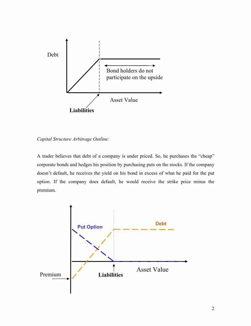
Capital Structure Arbitrage Outline:

A trader believes that debt of a company is under priced. So, he purchases the “cheap”

corporate bonds and hedges his position by purchasing puts on the stocks. If the company

doesn’t default, he receives the yield on his bond in excess of what he paid for the put

option. If the company does default, he would receive the strike price minus the

premium.

Asset Value

Debt

Liabilities

Bond holders do not participate on the upside

Asset Value

Debt

Premium Liabilities

Put Option

3

2. Debt Evaluation and Merton Model

2.1 Importance of Debt Valuation

The assessment of credit risk has always been important to banks and other financial

institutions. Recently banks have devoted even more resources to this task. This is

because regulatory credit-risk capital may be determined using a bank’s internal

assessments of the probabilities that its counter parties will default.

Since the capital structure of any firm is the sum of debt and equity, a fair valuation for

debt is essential to make financial markets more transparent and competitive. As long as

the debt market is not as developed as the equity market, arbitrage opportunities

stemming from the relative mispricing may exist. This can then be used to take advantage

of the imperfect debt pricing in the market. If operations are developed to link credit

market with equity and options markets, then the markets can become stronger and

appropriate debt risk hedging can be resorted to.

Now, the value of corporate debt depends on three items, namely,

1) The riskless rate of return, as observed from government bonds and very high-

grade corporate bonds.

2) The terms of reference contained in the indenture to the bond issue.

3) The probability that the firm may default on commitment to pay back the debt.

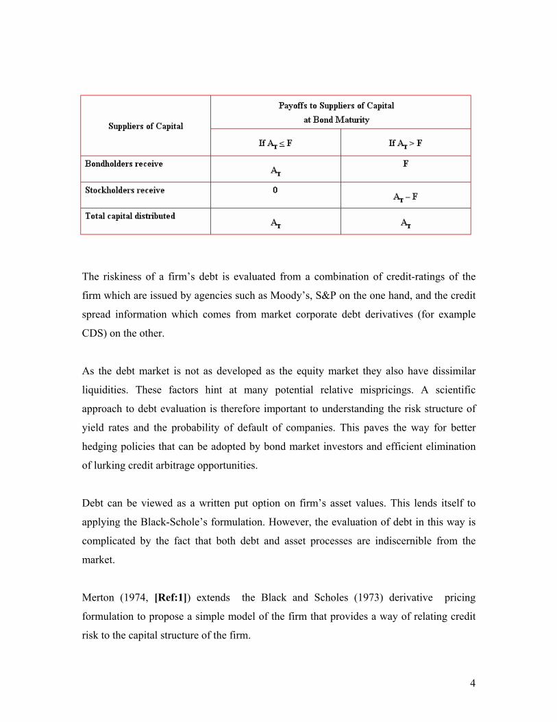
The corporate debt is thus risky, in that it is not as risk-free as government bonds and

there is the chance for default by the firm as it can go bankrupt. The debt holders have

first priority in the payment whenever the company becomes bankrupt as detailed below:

4

The riskiness of a firm’s debt is evaluated from a combination of credit-ratings of the

firm which are issued by agencies such as Moody’s, S&P on the one hand, and the credit

spread information which comes from market corporate debt derivatives (for example

CDS) on the other.

As the debt market is not as developed as the equity market they also have dissimilar

liquidities. These factors hint at many potential relative mispricings. A scientific

approach to debt evaluation is therefore important to understanding the risk structure of

yield rates and the probability of default of companies. This paves the way for better

hedging policies that can be adopted by bond market investors and efficient elimination

of lurking credit arbitrage opportunities.

Debt can be viewed as a written put option on firm’s asset values. This lends itself to

applying the Black-Schole’s formulation. However, the evaluation of debt in this way is

complicated by the fact that both debt and asset processes are indiscernible from the

market.

Merton (1974, [Ref:1]) extends the Black and Scholes (1973) derivative pricing

formulation to propose a simple model of the firm that provides a way of relating credit

risk to the capital structure of the firm.

5

2.2 Merton’s Model (1974)

Robert C. Merton developed a theory of risk structure of interest rates, which accounts

for price differentials between bonds to reflect the probability of default [Ref:1]. Merton

dealt with the theoretical basing of corporate debt pricing as an extension of Black-

Scholes’ general equilibrium theory of derivative pricing. The ability to formulate debt

price as a function of observable variables is the main attraction of this approach. This

essentially utilizes the directly observable equity process, by viewing equity as a call

option on firm’s assets to arrive at the underlying asset process.

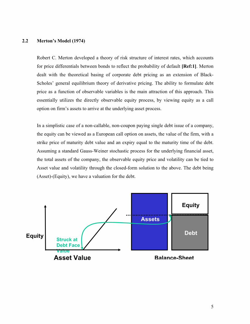
In a simplistic case of a non-callable, non-coupon paying single debt issue of a company,

the equity can be viewed as a European call option on assets, the value of the firm, with a

strike price of maturity debt value and an expiry equal to the maturity time of the debt.

Assuming a standard Gauss-Weiner stochastic process for the underlying financial asset,

the total assets of the company, the observable equity price and volatility can be tied to

Asset value and volatility through the closed-form solution to the above. The debt being

(Asset)-(Equity), we have a valuation for the debt.

Equity Debt

Assets

Equity

Struck at Debt Face Value

Asset Value Balance-Sheet

6

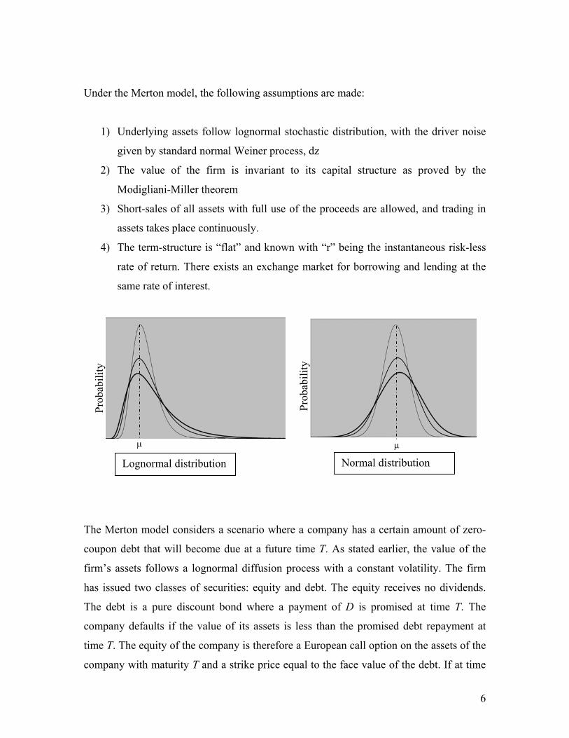
Under the Merton model, the following assumptions are made:

1) Underlying assets follow lognormal stochastic distribution, with the driver noise

given by standard normal Weiner process, dz

2) The value of the firm is invariant to its capital structure as proved by the

Modigliani-Miller theorem

3) Short-sales of all assets with full use of the proceeds are allowed, and trading in

assets takes place continuously.

4) The term-structure is “flat” and known with “r” being the instantaneous risk-less

rate of return. There exists an exchange market for borrowing and lending at the

same rate of interest.

The Merton model considers a scenario where a company has a certain amount of zero-

coupon debt that will become due at a future time T. As stated earlier, the value of the

firm’s assets follows a lognormal diffusion process with a constant volatility. The firm

has issued two classes of securities: equity and debt. The equity receives no dividends.

The debt is a pure discount bond where a payment of D is promised at time T. The

company defaults if the value of its assets is less than the promised debt repayment at

time T. The equity of the company is therefore a European call option on the assets of the

company with maturity T and a strike price equal to the face value of the debt. If at time

Prob

abili

ty

Prob

abili

ty

µ µ

Lognormal distribution Normal distribution

7

T, the firm’s asset value exceeds the promised payment, D, the lenders are paid the

promised amount and the shareholders receive all residual claims to the assets. If the

asset value is less than the promised payment the firm defaults, the lenders receive a

payment equal to the asset value, and the shareholders get nothing.

The model can be used to estimate either the risk-neutral probability that the company

will default or the credit spread on the debt. As inputs, Merton's model requires the

current value of the company's assets, the volatility of the company’s assets, the

outstanding debt, and the debt maturity. But as only the equity process can be observed in

the market, we can derive the underlying asset process from equity and then evaluate debt

and the credit-spread.

2.2.1 Equity Value and the Probability of Default

Let E represent the value of the firm’s equity and A the value of its assets. Let E0 & A0 be

the values of E and A today and let ET & AT be their values at time T. In the Merton

framework the payment to the shareholders at time T, is given by (a call option):

ET = max [AT – D, 0]

The underlying asset follows the following stochastic process, the driver noise being

given by standard normal Weiner process dz :

dA = µA dt + σAdz

The current equity price, therefore, can be immediately evaluated as a closed form

solution of the Black-Scholes’ PDE:

E0 = A0N(d1) − De –rT N(d2) ….. the closed form solution of Black-Scholes’ equation for

a European call option .

where

8

d1 = (ln (A0 e –rT/D) / (σA√T)) + 0.5σA √T ; d2 = d1 – 0.5 σA √T

where σA is the volatility of the asset value, and r is the risk-free rate of interest, both of

which are assumed to be constant. If D*= De –rT is the present value of the promised debt

payment and if L = D*/ A0 is the measure of leverage of the firm, then the equity value

is:

E0 = A0[N(d1) − LN(d2)] --------- (1)

It was shown by Jones et al (1984), that as the equity value is a function of the asset

value, Ito’s lemma can be used to determine the instantaneous volatility of the equity

from the asset volatility:

E0 σE = (∂E/∂A) A0 σA

where σE is the instantaneous volatility of the company’s equity at time zero. From

equation (1), this leads to

σE = (σAN(d1))/[N(d1) − LN(d2)] -------- (2)

Equations (1) and (2) allow A0 and σA to be obtained from E0, σE, L and T. The risk-

neutral probability, P, that the company will default by time T is the probability that

shareholders will not exercise their call option to buy the assets of the company for D at

time T. It is given by

P= N(-d2) --------- (3)

This depends only on the leverage, L, the asset volatility, σ, and the time to repayment, T.

9

2.2.2 Debt evaluation

As can be seen from above, debt (D) can then be evaluated, knowing that:

A= D + E

we have:

D0= A0[ N(-d1) + LN(d2)]

also,

Credit Spread ≈ y - r = -ln(N(d2)+ N(d1)/L]/T

This credit spread can then be compared with the corporate debt derivatives like Credit

Default Swaps, where a premium is paid by the protection buyer to the protection seller

who undertakes to pay the former in case of default by the reference company.

2.3 Shortcomings of Merton model

It is seen that the distributions of empirical returns do not precisely follow a lognormal

distribution upon which the above results are based. While of great importance and wide

acceptance, these theoretical option prices do not quite match the observed equity prices.

The Merton model underestimates the prices of away-from-the-money options. This

means that the implied volatilities of various strike prices form a convex function, rather

than the expected flat line. The empirical returns of stock, for example, are seen to have

fatter tails and skews when compared to the normal distribution. [Ref: 2, Lisa Borland]

10

3. The Non-Gaussian approach [Ref:3]

So, given the above shortcomings, several modifications to the Merton model have been

suggested in an attempt to correct the discrepancies. These approaches are often very

complicated and mostly ad-hoc. They seldom yielded manageable closed form solutions.

These approaches vary from the introduction of a stochastic model for the volatility of

stock price [Hull and White, 2003, Ref:4], to using a Poisson jump diffusion term to

describe extreme price movements.

Lisa Borland et al of EVA Funds, applied a non-Gaussian modification to the underlying

asset process which follows a Gaussian stochastic process in the traditional Merton

model.. This non-Gaussian stochastic process, called the Tsallis distribution, allows for

statistical feedback. These processes closely match the distributions of returns of stocks

and currency quotes, as found empirically. In our study, we undertake this approach as

described in following sections

3.1 Background

The stochastic model derives from a class of processes which have been recently

developed within the framework of statistical physics, more precisely the very active

field of Tsallis non-extensive thermo statistics. Lisa Borland applied the power-law

distributions characteristic of the Tsallis framework for the financial quantities.

11

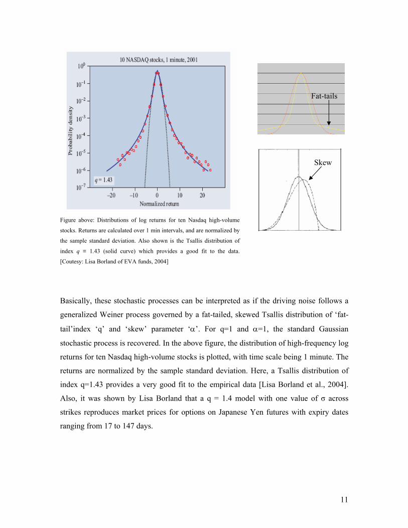
Figure above: Distributions of log returns for ten Nasdaq high-volume

stocks. Returns are calculated over 1 min intervals, and are normalized by

the sample standard deviation. Also shown is the Tsallis distribution of

index q = 1.43 (solid curve) which provides a good fit to the data.

[Coutesy: Lisa Borland of EVA funds, 2004]

Basically, these stochastic processes can be interpreted as if the driving noise follows a

generalized Weiner process governed by a fat-tailed, skewed Tsallis distribution of ‘fat-

tail’index ‘q’ and ‘skew’ parameter ‘α’. For q=1 and α=1, the standard Gaussian

stochastic process is recovered. In the above figure, the distribution of high-frequency log

returns for ten Nasdaq high-volume stocks is plotted, with time scale being 1 minute. The

returns are normalized by the sample standard deviation. Here, a Tsallis distribution of

index q=1.43 provides a very good fit to the empirical data [Lisa Borland et al., 2004].

Also, it was shown by Lisa Borland that a q = 1.4 model with one value of σ across

strikes reproduces market prices for options on Japanese Yen futures with expiry dates

ranging from 17 to 147 days.

Fat-tails

Skew

12

3.2 Application of Tsallis distribution to Merton model

Motivated by the good fit between the proposed model class and empirical data, Tsallis

non-Gaussian stochastic processes have been used to represent movements of the returns

of underlying stock and thus the underlying asset process. Generalized option pricing

formulas can then be derived using Black-Scholes’ formulation, so as to be able to obtain

fair values of derivatives of the underlying. Using these formulas we can expect to get a

good match with empirical observations of other derivative prices, like in our case, the

debt.

Adapting the Merton model as explained in Section 2.2, to the Tsallis stochastic process

for the underlying asset, we have:

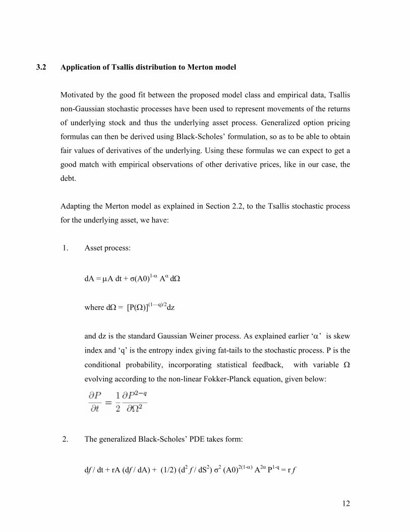
1. Asset process:

dA = µA dt + σ(A0)1-α Aα dΩ

where dΩ = [P(Ω)](1—q)/2dz

and dz is the standard Gaussian Weiner process. As explained earlier ‘α’ is skew

index and ‘q’ is the entropy index giving fat-tails to the stochastic process. P is the

conditional probability, incorporating statistical feedback, with variable Ω

evolving according to the non-linear Fokker-Planck equation, given below:

2. The generalized Black-Scholes’ PDE takes form:

df / dt + rA (df / dA) + (1/2) (d2 f / dS2) σ2 (A0)2(1-α) A2α P1-q = r f

13

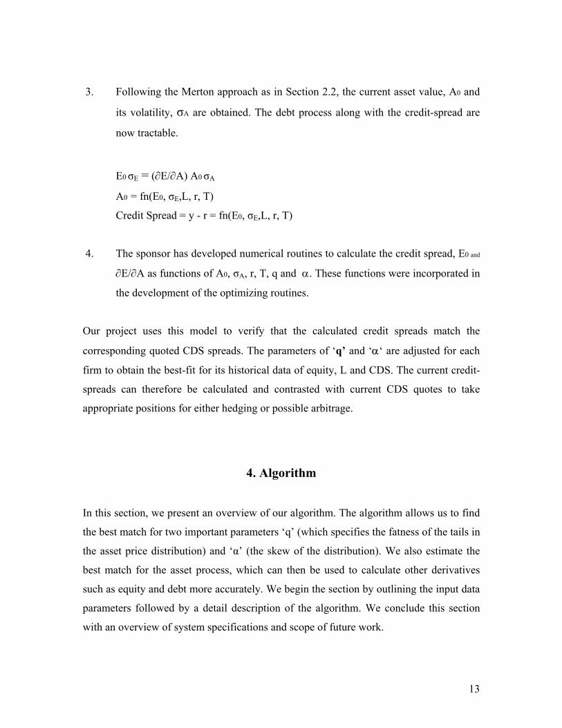
3. Following the Merton approach as in Section 2.2, the current asset value, A0 and

its volatility, σA are obtained. The debt process along with the credit-spread are

now tractable.

E0 σE = (∂E/∂A) A0 σA

A0 = fn(E0, σE,L, r, T)

Credit Spread = y - r = fn(E0, σE,L, r, T)

4. The sponsor has developed numerical routines to calculate the credit spread, E0 and

∂E/∂A as functions of A0, σA, r, T, q and α. These functions were incorporated in

the development of the optimizing routines.

Our project uses this model to verify that the calculated credit spreads match the

corresponding quoted CDS spreads. The parameters of ‘q’ and ‘α‘ are adjusted for each

firm to obtain the best-fit for its historical data of equity, L and CDS. The current credit-

spreads can therefore be calculated and contrasted with current CDS quotes to take

appropriate positions for either hedging or possible arbitrage.

4. Algorithm

In this section, we present an overview of our algorithm. The algorithm allows us to find

the best match for two important parameters ‘q’ (which specifies the fatness of the tails in

the asset price distribution) and ‘α’ (the skew of the distribution). We also estimate the

best match for the asset process, which can then be used to calculate other derivatives

such as equity and debt more accurately. We begin the section by outlining the input data

parameters followed by a detail description of the algorithm. We conclude this section

with an overview of system specifications and scope of future work.

14

In this algorithm, we seek to verify how “fair” the corporate debt instruments are priced

relative to their equity prices and asset value in the market. For this purpose, we compute

the Credit Default Swap (CDS) spreads from various data parameters and compare them

to the available CDS quotes in the market. The q and α parameters are then obtained as a

best fit to reduce the error between the two CDS values. In this process, we also come up

with a better approximation to the asset value of the company.

4.1 Input Data Parameters

Several data parameters are used as inputs to compute the CDS value in our algorithm.

The particulars of data selection are detailed in the DATA section of the report. We

denote data parameters with symbols within ( ) for ease in understanding the algorithm:

a) Market CDS quotes (CDSq)

b) Equity prices (E)

c) Equity Volatility (σE)

d) Total book value of assets (A)

e) Asset Volatility (σA)

f) Book value of long term debt (D)

g) Risk free rate (r)

h) Time to maturity of Debt (T)

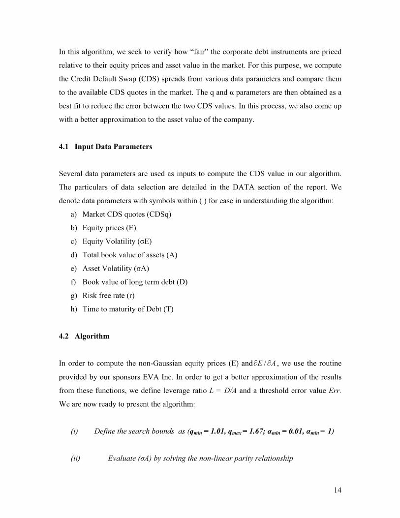
4.2 Algorithm

In order to compute the non-Gaussian equity prices (E) and AE ∂∂ / , we use the routine

provided by our sponsors EVA Inc. In order to get a better approximation of the results

from these functions, we define leverage ratio L = D/A and a threshold error value Err.

We are now ready to present the algorithm:

(i) Define the search bounds as (qmin = 1.01, qmax = 1.67; αmin = 0.01, αmin = 1)

(ii) Evaluate (σA) by solving the non-linear parity relationship

15

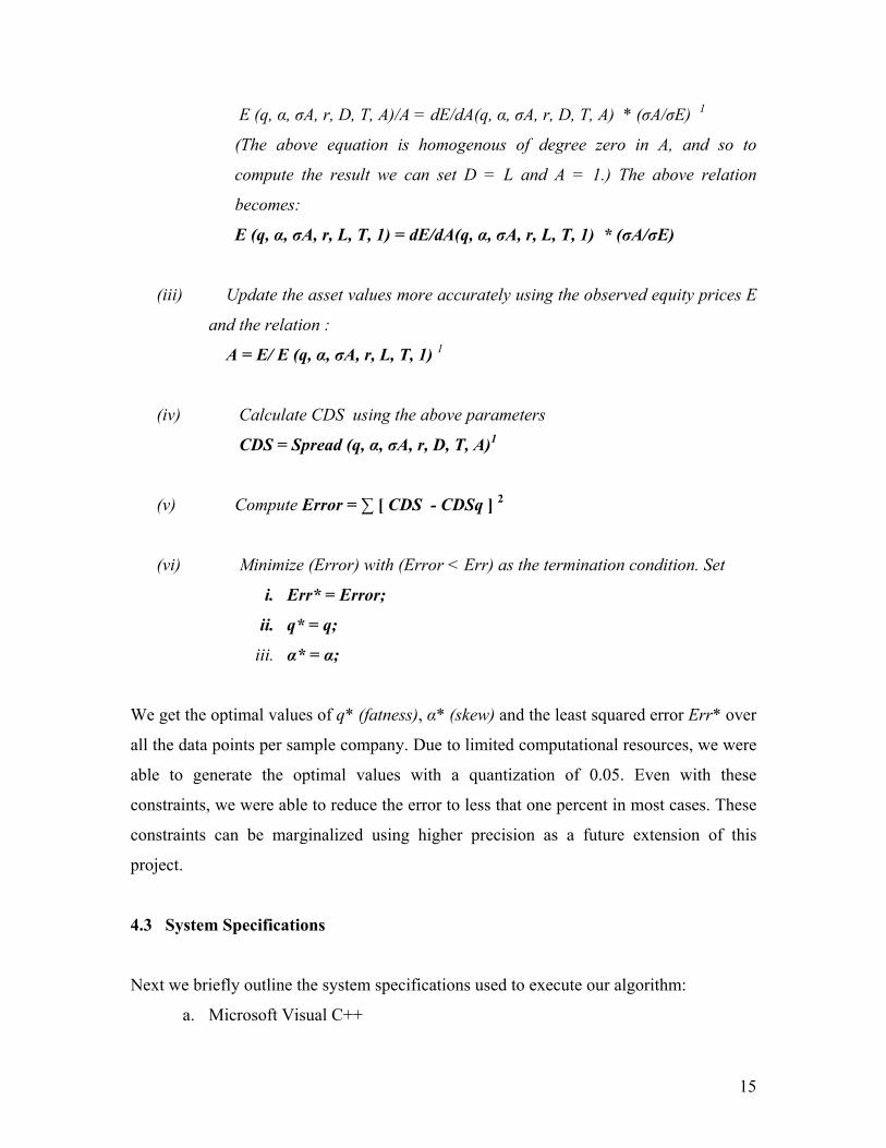
E (q, α, σA, r, D, T, A)/A = dE/dA(q, α, σA, r, D, T, A) * (σA/σE) 1

(The above equation is homogenous of degree zero in A, and so to

compute the result we can set D = L and A = 1.) The above relation

becomes:

E (q, α, σA, r, L, T, 1) = dE/dA(q, α, σA, r, L, T, 1) * (σA/σE)

(iii) Update the asset values more accurately using the observed equity prices E

and the relation :

A = E/ E (q, α, σA, r, L, T, 1) 1

(iv) Calculate CDS using the above parameters

CDS = Spread (q, α, σA, r, D, T, A)1

(v) Compute Error = ∑ [ CDS - CDSq ] 2

(vi) Minimize (Error) with (Error < Err) as the termination condition. Set

i. Err* = Error;

ii. q* = q;

iii. α* = α;

We get the optimal values of q* (fatness), α* (skew) and the least squared error Err* over

all the data points per sample company. Due to limited computational resources, we were

able to generate the optimal values with a quantization of 0.05. Even with these

constraints, we were able to reduce the error to less that one percent in most cases. These

constraints can be marginalized using higher precision as a future extension of this

project.

4.3 System Specifications

Next we briefly outline the system specifications used to execute our algorithm:

a. Microsoft Visual C++

16

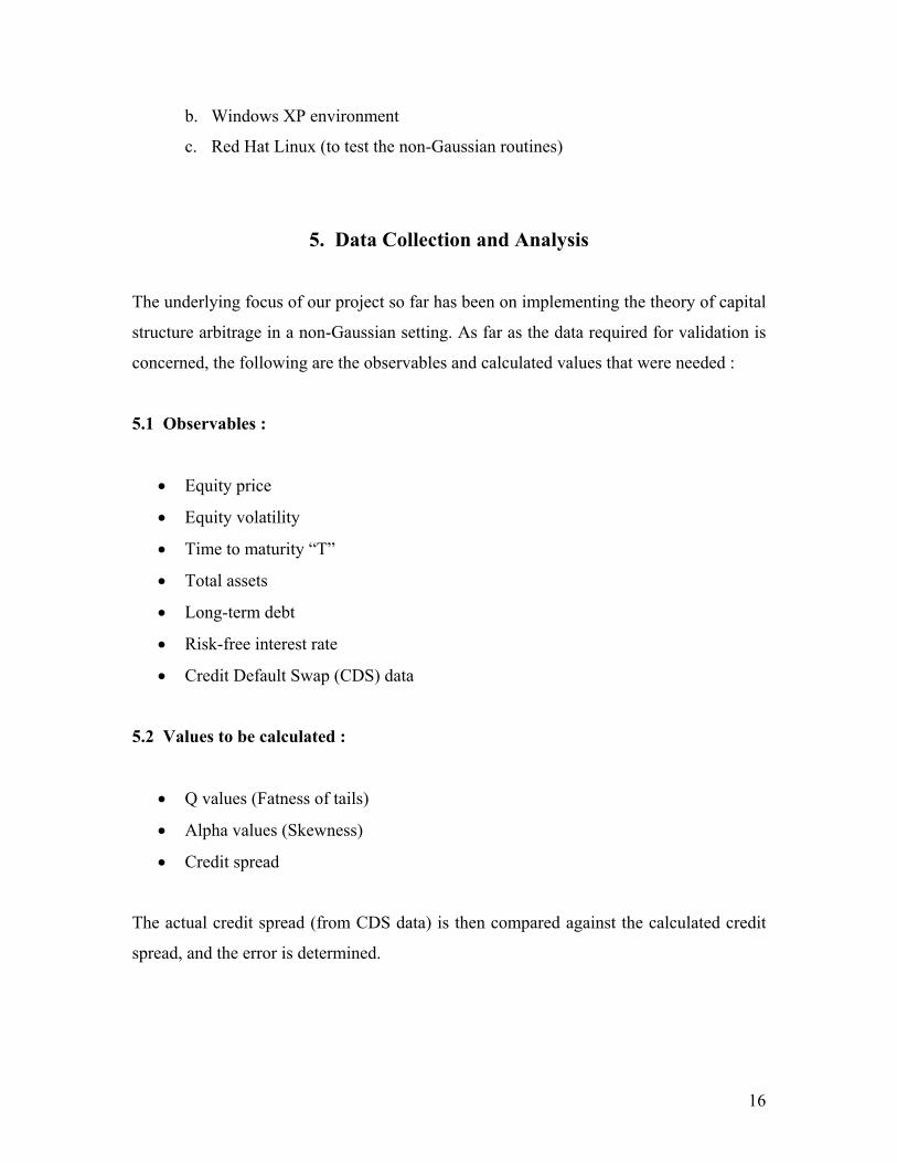
b. Windows XP environment

c. Red Hat Linux (to test the non-Gaussian routines)

5. Data Collection and Analysis The underlying focus of our project so far has been on implementing the theory of capital

structure arbitrage in a non-Gaussian setting. As far as the data required for validation is

concerned, the following are the observables and calculated values that were needed :

5.1 Observables :

• Equity price

• Equity volatility

• Time to maturity “T”

• Total assets

• Long-term debt

• Risk-free interest rate

• Credit Default Swap (CDS) data

5.2 Values to be calculated :

• Q values (Fatness of tails)

• Alpha values (Skewness)

• Credit spread

The actual credit spread (from CDS data) is then compared against the calculated credit

spread, and the error is determined.

17

5.3 Credit Default Swaps Data

The basic advantage of these credit default swaps is that they provide insurance against a

default by a particular company or sovereign entity. In theory, CDS data are close to the

credit spread of the yield on an n-year par yield bond issued by the reference entity over

n-year par yield risk-free rate.

CDS quotes were taken for 1,3,5,7 and 10-year periods at each of 16 data points for each

quarter of a 4 year period from January 2000 to December 2003. CDS quotes over a five

year period were given courtesy Lombard Data Systems. CDS quotes for each company

were taken according to the time to maturity of its bonds.

The following is a list of the various symbols used in the CDS data quotes along with a

few examples :

ValuSpread Ticker : Ticker symbol

Full Name : The full reference entity name

Rank : The rank of the debt for which the protection is valid. Sovereign

debt is assigned no rank.

Curr : The currency of the debt for which the protection is valid

Restruct : The restructuring rules of the credit protection

CUMR – “With Restructuring” Credit spreads will include a

premium for full restructuring.

XMMR – “Modified-Modified Restructuring” Until CUMR

contracts expire, both CUMR & XMMR spreads will be quoted.

18

MODR – “Modified Restructuring” Credit spreads will include a

premium for modified restructuring.

EXR – “Excluding Restructuring” Credit spreads will exclude any

type of debt restructuring premium.

Mid/Recovery : Defines whether the value in the column titled ‘LRS Mean’ is a

mid-market mean credit spread (CDM) or a recovery rate (CDR).

Both values are derived from the contributions of key market

makers in the credit derivatives market.

Maturity : The maturity of the protection. For this reason, recovery rates

identified in the ‘Mid/Recovery’ column have no maturity.

LRS Mean : Either a mid-market mean or a mean recovery rate as defined in

‘Mid/Recovery’. Values are quoted in basis points and are rounded

to two decimal places.

LRS Std Dev : The degree of variability of the contributions, rounded to two

decimal places.

Date : The date on which the credit spread /recovery rate has been valued.

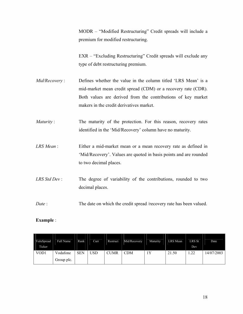
Example :

ValuSpread

Ticker

Full Name

Rank

Curr

Restruct

Mid/Recovery

Maturity

LRS Mean

LRS St

Dev

Date

VOD1 Vodafone

Group plc.

SEN USD CUMR CDM 1Y 21.50 1.22 14/07/2003

19

• The unique ticker is VOD1 and the company under consideration is Vodafone

Group plc.

• Data is applicable to senior debt that is denominated in US Dollars.

• The restructuring type is CUMR. (with restructuring)

• The mean is a mid-market mean credit spread.

• Data is applicable to 1 year protection.

• The mid-market mean derived from market makers contributions is 21.50 basis

points.

• The standard deviation of those contributions is 1.22

• The data is applicable to the 14th of July 2003.

5.4 Equity Data

• Equity prices were taken from January 2000 to December 2003.

• Adjusted closing price was taken for this purpose.

• Historic volatility was estimated using the daily stock prices of that particular

quarter

• Using a quarter to estimate volatility is a trade-off. Using a longer period to

estimate volatility would result in a more accurate but less timely estimate, while

using a shorter period would result in less accurate but more timely estimate.

• Equity prices were taken from http://finance.yahoo.com

5.5 Balance Sheet Data

• Total assets (book value) were taken for each company at each data-point.

20

• Long-term debt (book value) was taken for each company at each data-point.

• Asset and debt-values were taken from CompuStat.

5.6 Interest Rate and ‘T’

• Risk-free interest rates were taken for each of the 16 data-points.

• Risk-free interest rate for 1,3,5,7 and 10-year periods were taken.

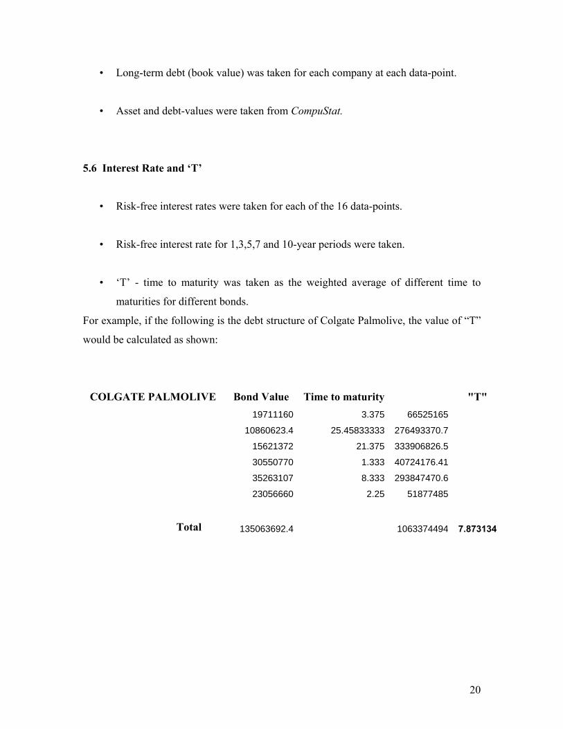
• ‘T’ - time to maturity was taken as the weighted average of different time to

maturities for different bonds.

For example, if the following is the debt structure of Colgate Palmolive, the value of “T”

would be calculated as shown:

COLGATE PALMOLIVE Bond Value Time to maturity "T"

19711160 3.375 66525165

10860623.4 25.45833333 276493370.7

15621372 21.375 333906826.5

30550770 1.333 40724176.41

35263107 8.333 293847470.6

23056660 2.25 51877485

Total 135063692.4 1063374494 7.873134

21

5.7 Merging the Data

• In total, 54 companies were chosen across various sectors such as Retail,

Communication, Aerospace, Finance, Energy, etc.

• The companies were chosen across various sectors just to validate the model

against various types of industries.

• Also, one of the criteria to choose companies was that the CDS data over the

entire period should be available to us.

• For each company, there were 16 data points – quarter-end points from January

2000 to December 2003.

• Companies were chosen with different market cap sizes and grouped as under 3

classes :

a) Large Cap (Total Assets > $50 billion)

b) Medium Cap ($10 billion < Total Assets < $50 billion)

c) Small Cap (Total Assets < $10 billion)

A sample input file for a single company would thus consist of the following :

a) Equity volatilities (16 data points : 4 yrs * 4 qtrs)

b) Equity prices (16 data points : 4 yrs * 4 qtrs)

c) Asset value (16 data points : 4 yrs * 4 qtrs)

d) Long term Debt (16 data points : 4 yrs * 4 qtrs)

e) Risk free rate (80 data points : 1,3,5,7 &10 yr rate for 16 quarters)

f) CDS quotes (80 data points : 1,3,5,7 &10 yr rate for 16 quarters)

22

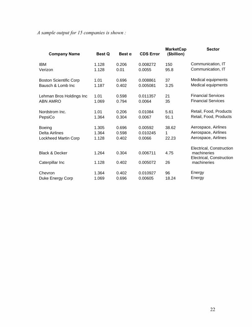
A sample output for 15 companies is shown :

Company Name Best Q Best α CDS Error MarketCap ($billion)

Sector

IBM 1.128 0.206 0.008272 150 Communication, IT Verizon 1.128 0.01 0.0055 95.8 Communication, IT Boston Scientific Corp 1.01 0.696 0.008861 37 Medical equipments Bausch & Lomb Inc 1.187 0.402 0.005081 3.25 Medical equipments Lehman Bros Holdings Inc 1.01 0.598 0.011357 21 Financial Services ABN AMRO 1.069 0.794 0.0064 35 Financial Services Nordstrom Inc. 1.01 0.206 0.01084 5.61 Retail, Food, Products PepsiCo 1.364 0.304 0.0067 91.1 Retail, Food, Products Boeing 1.305 0.696 0.00592 38.62 Aerospace, Airlines Delta Airlines 1.364 0.598 0.010245 1 Aerospace, Airlines Lockheed Martin Corp 1.128 0.402 0.0066 22.23 Aerospace, Airlines

Black & Decker 1.264 0.304 0.006711 4.75 Electrical, Construction machineries

Caterpillar Inc 1.128 0.402 0.005072 26 Electrical, Construction machineries

Chevron 1.364 0.402 0.010927 96 Energy Duke Energy Corp 1.069 0.696 0.00605 18.24 Energy

23

6. Hedging and Capital Structure Arbitrage 6.1 Credit Risk Hedging Strategies

In this section, the process of Omicron Neutral Hedging is explained in some detail.

Further, the implied exploitation of credit pricing discrepancies is discussed.

A regular hedged position includes the assumption of positions that neutralize the risk

involved in asset claims that are contingent on an uncertain underlier. Consider the

example of a trivial currency hedge. Consider the parity of a certain currency to the US

Dollar to be X/$. The position of simultaneously selling $1 for X of the foreign currency

and selling X back of the same currency for US Dollars bears no inherent currency rate

risk. Further, should there be an arbitrage opportunity, this pair of transactions will

produce a non-zero cash flow. A negative cash flow in this scenario can elementarily be

exploited by taking the opposite side of the transactions described above. Also, if the

trade is not simultaneous, the returns from this pair of trades should match the

corresponding risk-free rate.

Analogous to this example is the case of a credit risk hedge. The derivative that is

relevant to the credit risk is the Omicron (dE/d(OAS)).

The risk-neutralizing transaction of a position with positive Omicron would involve

assuming an equivalent position in CDS contracts. There could be two different reasons

to assume this position as described below:

1. The combination of transactions simply aims to relieve the bearer of any credit

risk of the underlier. Consider a speculative trade involving the bond issue of a

particular company. The assumption of the prescribed trade, assuming the CDS

spread is fair-priced, relieves the speculator of the risk involved in holding the

risky corporate debt.

2. The Omicron neutral position can be used to exploit any credit arbitrage

opportunity. Consider the following transaction: This is a modification of the

delta neutral Convertible Bond arbitrage technique. A convertible bond purchase

24

is made for a certain sum. The corresponding short delta position is taken in the

stock.

Consider an instrument with an Omicron value of O. Now entering into the

appropriate CDS contract will make the portfolio Omicron neutral. Thus for a

small change in the credit spread of dS, the value of the instrument falls by O*dS.

However, the value of the CDS contract held increases by the same O*dS (by

definition of the hedge), leaving the value of the portfolio unchanged. In the

presence of any mis-pricing, this pair of trades would have a non-zero initial cash

flow, producing a return of zero. The portfolio will naturally have to be

rebalanced in order to maintain the optimum hedge position.

As it is essential to correctly estimate the optimal hedge at every instant, the Omicron

derivative must be obtained by the best possible estimate. This is where the non-Gaussian

model can be applied. If a better understanding of the underlying asset process is forded

by using the non-Gaussian model discussed in this report, this should in fact be employed

in the derivative estimation.

It is important to note that the process of extracting value from any potential credit risk

mis-pricing may involve assuming other risks such as interest rate risk, currency risk or

market risk. These positions can and must therefore also be appropriately hedged in order

to be assured of an arbitrage return.

6.2 Note on Market Correction

Theoretically, the continuous rebalancing strategy presented above does not require a

“market correction”. This is because the value of the terminal value of the CDS contract

is unambiguous at maturity. Hence, the valuation is necessarily “correct” at this time-

point. To make a certain gain from any mis-pricing by the above technique, the trade

positions must be designed to extract a positive cash flow from any mis-pricing at each

rebalancing. This also generates the maximal cash flow from any credit risk mis-pricing.

If the market does “correct” at a time before maturity following a previous mis-pricing,

the arbitrage can be terminated at this point by closing out all positions.

25

7. Results and Conclusions

7.1 Results

The available data was processed for the complete sample set of companies and the

algorithm delineated above was used to identify the model parameters for each sample.

The results of the algorithm were analyzed from different perspectives.

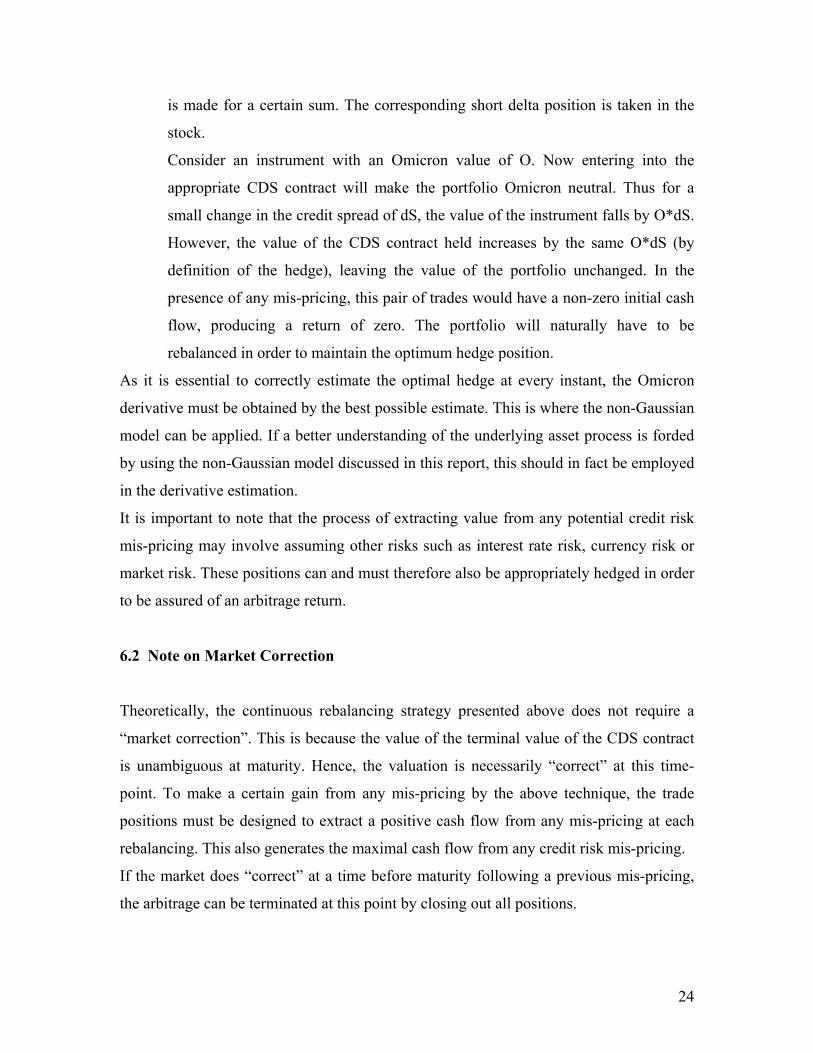
First, the q values are presented against companies sorted by market capitalization.

Analyzing all the samples, the overall average qavg = 1.23 and αavg = 0.3. These values

provide a zeroth order estimate to evaluate asset processes. While there is a moderate

departure from the Gaussian case indicated by the value of q (against q=1, for Gaussian

processes), the α value presents a significant skew compared to the normal case of α=1.

The (q, α) values were tested for predictability. As is apparent from the graph above,

almost all ranges of q are assumed by different companies in each market size. The first

Q Values

1

1.2

1.4

1.6

0 10 20 30 40 50 60

Samples (Large - Small Cap)

Q

26

series represents largest size companies and can be seen to take on a more conservative

range of q values compared to relatively smaller companies.

Best Alpha

0

0.1

0.2

0.3

0.4

0.5

0.6

0.7

0.8

0.9

Market Cap Ranges (Large, Mid, Small)

Best Alpha

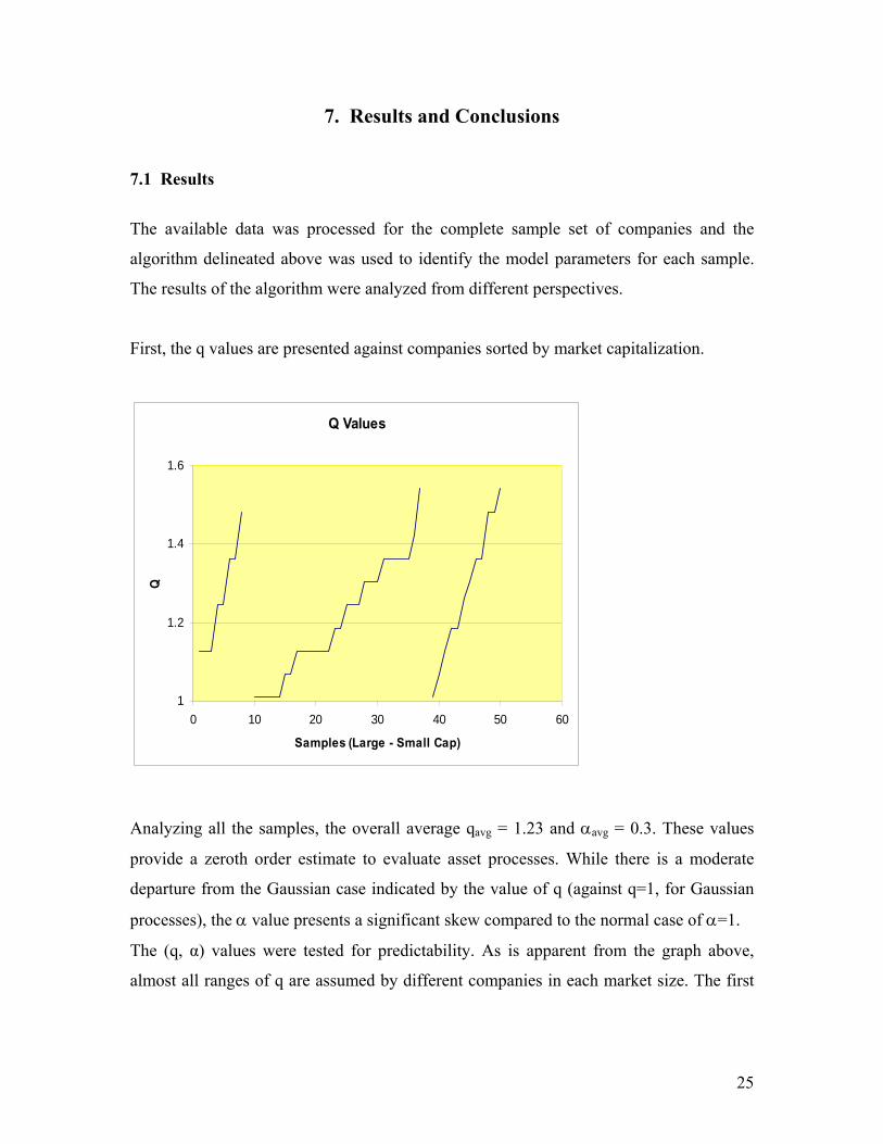
In this graph, it is seen that the α values take on greater departures from normalcy on

larger companies. In fact, no company in this range shows a value near 1. This can be

explained in part by the non-Gaussian model characterization. When the Asset variance

(σ), the Asset Value and α are all fit to available data, a larger asset value could be

supported by a combination of a smaller α and a larger σ. This does not present a

discrepancy. This structure shows the possible set of actual values that cause the

derivative processes and properties (Equity values, CDS spreads and volatility) as

observed. This might have to do with the fact that large companies’ volatilities reflect a

belief of larger Asset Values than in the Gaussian case.

The values for (q, α) and Asset Volatility obtained in our analyses are smaller than those

expected based on evaluations on Equity prices. This is understandable as the Asset

27

process includes both debt and equity and the overall process can be expected to have

lower percentage volatility when compared to the equity portion alone.

The next data characterization exercise involves identifying potential patterns that would

allow a combined joint estimation of (q, α) based on some single representative

evaluation.

The scatter plot above shows that there is no perceptible pattern as described above. This

hints at the relative independence of these parameters. Hence (q, α) need to be evaluated

independently, justifying the process described in the algorithm section that was used in

our analysis.

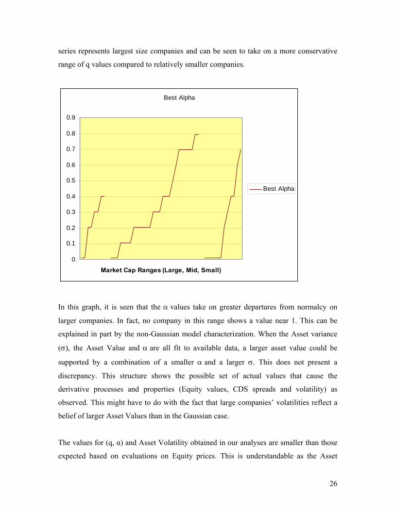
7.2 Sector Analysis

Further analyzing the q values obtained with respect to the sector-wise characterization of

samples, the following behavior is presented.

Q vs.

0

0.1

0.2

0.3

0.4

0.5

0.6

0.7

0.8

0.9

1 1.2 1.4 1.6

Q

Alp

ha

α

28

The qavg over the entire sample space seems to be representative of the qavg for each

sector. This reaffirms the sector-wise stability of the q values. With in each industry, the

full range of q-values seems to be assumed, indicating independence of these values from

sector information.

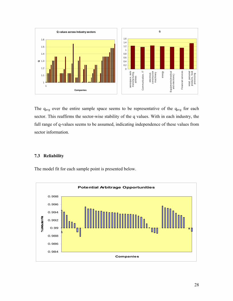
7.3 Reliability

The model fit for each sample point is presented below.

Q

00.20.40.60.8

11.21.41.6

aero

spac

e, a

uto

man

ufac

turin

g,ai

rline

s

Com

mun

icat

ion,

IT

elec

trica

l,co

nstru

ctio

nm

achi

nery

ener

gy

Equ

ipm

ents

(med

ical

and

elec

troni

c)

Fina

ncia

l ser

vice

s

reta

il, p

erso

nal

prod

ucts

, foo

dpr

oces

sing

Q values across Industry sectors

1

1.1

1.2

1.3

1.4

1.5

1.6

1

Companies

Q

Potential Arbitrage Opportunities

0.984

0.986

0.988

0.99

0.992

0.994

0.996

0.998

1

Companies

% M

odel F

it

29

The (q, α) parameters seem to be quite effective in matching the CDS values against

which they were evaluated. This justifies the use of the non-Gaussian model. A time

stability analysis of the fit would reaffirm the strength of this model. This however is a

task that needs to be addressed in possible extensions of this project. Studies by the

sponsor have shown that the parameter values are quite stable for a given target company.

This lends credibility to any indications provided by this model.

The outliers in terms of fit are quite clearly identifiable in the above graph. These

samples are ideal targets for investigation of possible capital structure mis-pricing.

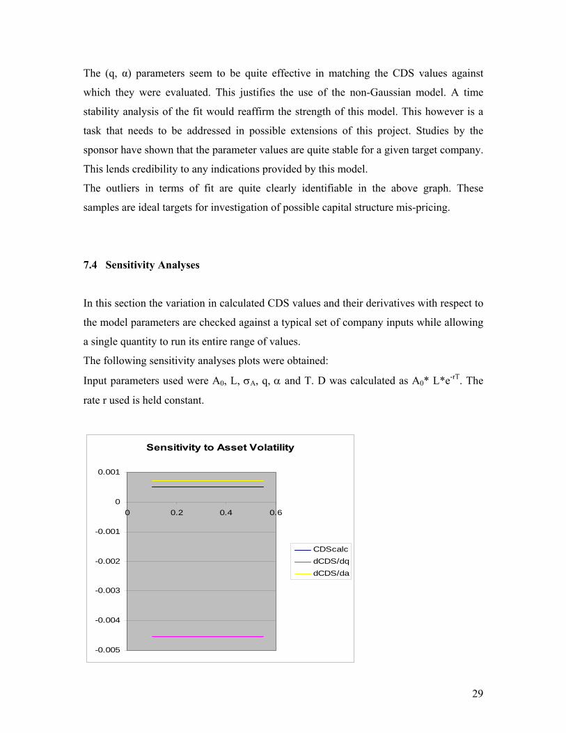
7.4 Sensitivity Analyses

In this section the variation in calculated CDS values and their derivatives with respect to

the model parameters are checked against a typical set of company inputs while allowing

a single quantity to run its entire range of values.

The following sensitivity analyses plots were obtained:

Input parameters used were A0, L, σA, q, α and T. D was calculated as A0* L*e-rT. The

rate r used is held constant.

Sensitivity to Asset Volatility

-0.005

-0.004

-0.003

-0.002

-0.001

0

0.001

0 0.2 0.4 0.6

CDScalcdCDS/dqdCDS/da

30

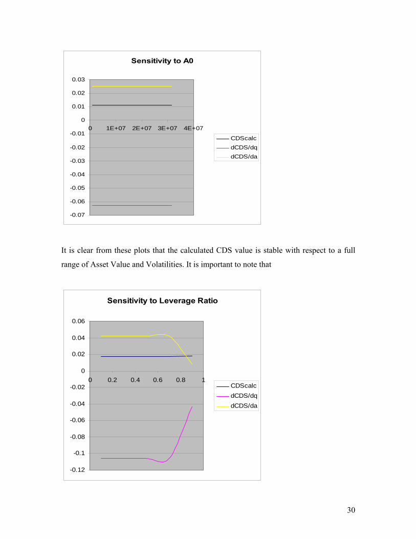
Sensitivity to A0

-0.07

-0.06

-0.05

-0.04

-0.03

-0.02

-0.01

0

0.01

0.02

0.03

0 1E+07 2E+07 3E+07 4E+07

CDScalcdCDS/dqdCDS/da

It is clear from these plots that the calculated CDS value is stable with respect to a full

range of Asset Value and Volatilities. It is important to note that

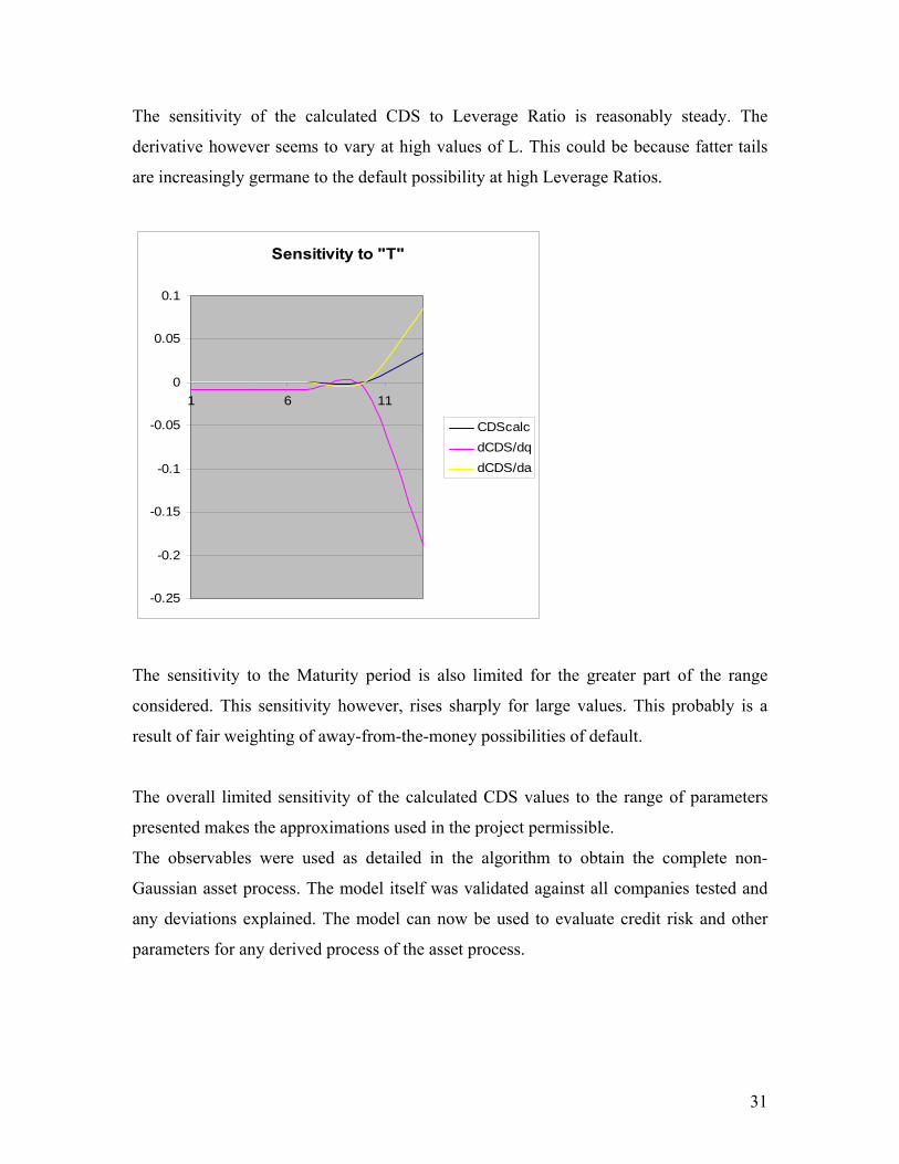
Sensitivity to Leverage Ratio

-0.12

-0.1

-0.08

-0.06

-0.04

-0.02

0

0.02

0.04

0.06

0 0.2 0.4 0.6 0.8 1CDScalcdCDS/dqdCDS/da

31

The sensitivity of the calculated CDS to Leverage Ratio is reasonably steady. The

derivative however seems to vary at high values of L. This could be because fatter tails

are increasingly germane to the default possibility at high Leverage Ratios.

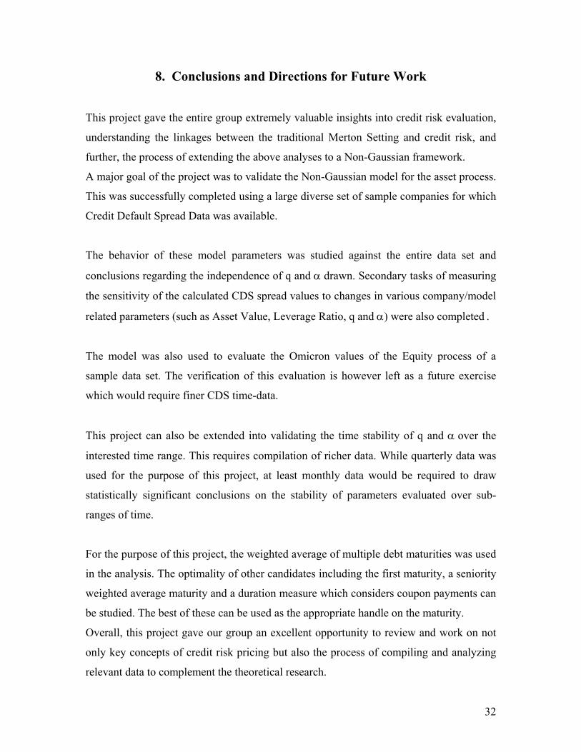
Sensitivity to "T"

-0.25

-0.2

-0.15

-0.1

-0.05

0

0.05

0.1

1 6 11

CDScalcdCDS/dqdCDS/da

The sensitivity to the Maturity period is also limited for the greater part of the range

considered. This sensitivity however, rises sharply for large values. This probably is a

result of fair weighting of away-from-the-money possibilities of default.

The overall limited sensitivity of the calculated CDS values to the range of parameters

presented makes the approximations used in the project permissible.

The observables were used as detailed in the algorithm to obtain the complete non-

Gaussian asset process. The model itself was validated against all companies tested and

any deviations explained. The model can now be used to evaluate credit risk and other

parameters for any derived process of the asset process.

32

8. Conclusions and Directions for Future Work

This project gave the entire group extremely valuable insights into credit risk evaluation,

understanding the linkages between the traditional Merton Setting and credit risk, and

further, the process of extending the above analyses to a Non-Gaussian framework.

A major goal of the project was to validate the Non-Gaussian model for the asset process.

This was successfully completed using a large diverse set of sample companies for which

Credit Default Spread Data was available.

The behavior of these model parameters was studied against the entire data set and

conclusions regarding the independence of q and α drawn. Secondary tasks of measuring

the sensitivity of the calculated CDS spread values to changes in various company/model

related parameters (such as Asset Value, Leverage Ratio, q and α) were also completed .

The model was also used to evaluate the Omicron values of the Equity process of a

sample data set. The verification of this evaluation is however left as a future exercise

which would require finer CDS time-data.

This project can also be extended into validating the time stability of q and α over the

interested time range. This requires compilation of richer data. While quarterly data was

used for the purpose of this project, at least monthly data would be required to draw

statistically significant conclusions on the stability of parameters evaluated over sub-

ranges of time.

For the purpose of this project, the weighted average of multiple debt maturities was used

in the analysis. The optimality of other candidates including the first maturity, a seniority

weighted average maturity and a duration measure which considers coupon payments can

be studied. The best of these can be used as the appropriate handle on the maturity.

Overall, this project gave our group an excellent opportunity to review and work on not

only key concepts of credit risk pricing but also the process of compiling and analyzing

relevant data to complement the theoretical research.

33

REFERENCES

[1] R.C. Merton, On the Pricing of Corporate Debt: The Risk Structure of Interest

Rates, Journal of Finance 29, 449-470, (May 1974)

[2] L. Borland, A Theory of non-Gaussian Option Pricing, Quantitative Finance 2,

415-431, (2002)

[3] L. Borland and J.P. Bouchaud, A Non-Gaussian Option Pricing Model with Skew,

to appear in Quantitative Finance (2004)

[4] J. Hull, I. Nelken, A. White, Merton's Model, Credit Risk, and Volatility Skews,

working paper, Jan 2004

[5] Oliver Berndt and Bruno Stephan Veras de Melo, Capital Structure Arbitrage

Strategies: Models, Practice and Empirical Evidence, Masters Thesis, Institute of

Banking and Finance, Lausanne, Switzerland (November 2003)