Essays in US Fiscal PolicyThe Harvard community has made this

article openly available. Please share howthis access benefits you. Your story matters

Citation Mahon, James. 2015. Essays in US Fiscal Policy. Doctoraldissertation, Harvard University, Graduate School of Arts &Sciences.

Citable link http://nrs.harvard.edu/urn-3:HUL.InstRepos:17463977

Terms of Use This article was downloaded from Harvard University’s DASHrepository, and is made available under the terms and conditionsapplicable to Other Posted Material, as set forth at http://nrs.harvard.edu/urn-3:HUL.InstRepos:dash.current.terms-of-use#LAA

Essays in US Fiscal Policy

A dissertation presented

by

James F. Mahon III

to

The Department of Political Economy and Government

in partial fulfillment of the requirements

for the degree of

Doctor of Philosophy

in the subject of

Political Economy and Government

Harvard University

Cambridge, Massachusetts

March 2015

c© 2015 James F. Mahon III

All rights reserved.

Dissertation Advisors:Professor Raj ChettyProfessor Edward Glaeser

Author:James F. Mahon III

Essays in US Fiscal Policy

Abstract

This dissertation presents three chapters about US tax and spending policy. The first chapter

investigates the take-up of a tax refund for corporate losses. We find that few firms claim

the refund despite that it dominates the alternative option. This finding indicates that many

firms fail to optimize perfectly with respect to taxes. The second chapter estimates corporate

responses to a tax incentive for investment. We find the largest responses among small

firms and firms without an alternative tax shield, suggesting that the tax incentive operates

through both the price and cash mechanisms. The third chapter tests for partisan effects on

the distribution of federal spending within congressional districts. Even when conditioning

on institutional contexts with greater partisan influence, I find little evidence that parties tilt

the distribution of federal spending to favor co-partisan and swing voters.

iii

Contents

Abstract . . . . . . . . . . . . . . . . . . . . . . . . . . . . . . . . . . . . . . . . . . . . iiiAcknowledgments . . . . . . . . . . . . . . . . . . . . . . . . . . . . . . . . . . . . . vii

Introduction 1

1 The Role of Experts in Fiscal Policy Transmission 31.1 Introduction . . . . . . . . . . . . . . . . . . . . . . . . . . . . . . . . . . . . . . 31.2 Corporate Losses and Tax Refunds . . . . . . . . . . . . . . . . . . . . . . . . . 8

1.2.1 The Tax Code’s Loss Rules . . . . . . . . . . . . . . . . . . . . . . . . . 81.2.2 Business Tax Data . . . . . . . . . . . . . . . . . . . . . . . . . . . . . . 101.2.3 Low Take-up of Tax Refunds for Losses . . . . . . . . . . . . . . . . . . 14

1.3 Evidence on Tax Loss Choices . . . . . . . . . . . . . . . . . . . . . . . . . . . . 171.3.1 A Cost-Benefit Analysis of Tax Loss Choices . . . . . . . . . . . . . . . 171.3.2 Empirical Evaluation of Cost-Benefit Formulas . . . . . . . . . . . . . 181.3.3 Alternative Explanations for Low Take-Up . . . . . . . . . . . . . . . . 24

1.4 Tax Preparers and the Take-up of Tax Refunds . . . . . . . . . . . . . . . . . . 261.4.1 Corporate Market for Tax Preparation Services . . . . . . . . . . . . . 271.4.2 Claiming Decisions and Preparer Characteristics . . . . . . . . . . . . 271.4.3 Variance of Unobserved Preparer Effect . . . . . . . . . . . . . . . . . . 39

1.5 Conclusion . . . . . . . . . . . . . . . . . . . . . . . . . . . . . . . . . . . . . . . 44

2 Do Financial Frictions Amplify Fiscal Policy? Evidence from Business InvestmentStimulus 462.1 Introduction . . . . . . . . . . . . . . . . . . . . . . . . . . . . . . . . . . . . . . 462.2 Hypothesis Development . . . . . . . . . . . . . . . . . . . . . . . . . . . . . . 522.3 Business Tax Data . . . . . . . . . . . . . . . . . . . . . . . . . . . . . . . . . . . 572.4 The Effect of Bonus Depreciation on Investment . . . . . . . . . . . . . . . . . 622.5 Explaining the Large Response with Financial Frictions . . . . . . . . . . . . . 80

2.5.1 Heterogeneous Responses by Ex Ante Financial Constraints . . . . . . 812.5.2 Heterogeneous Responses by Tax Position . . . . . . . . . . . . . . . . 842.5.3 Discount Rates and the Shadow Cost of Funds . . . . . . . . . . . . . . 88

iv

2.6 Conclusion . . . . . . . . . . . . . . . . . . . . . . . . . . . . . . . . . . . . . . . 92

3 Do the Victors Share the Spoils? Evidence from US House Elections, 1982-2006 943.1 Introduction . . . . . . . . . . . . . . . . . . . . . . . . . . . . . . . . . . . . . . 943.2 Motivation . . . . . . . . . . . . . . . . . . . . . . . . . . . . . . . . . . . . . . . 1003.3 Data and descriptive statistics . . . . . . . . . . . . . . . . . . . . . . . . . . . . 103

3.3.1 US counties panel . . . . . . . . . . . . . . . . . . . . . . . . . . . . . . 1033.3.2 Sample selection . . . . . . . . . . . . . . . . . . . . . . . . . . . . . . . 1053.3.3 Descriptive statistics . . . . . . . . . . . . . . . . . . . . . . . . . . . . . 106

3.4 Results . . . . . . . . . . . . . . . . . . . . . . . . . . . . . . . . . . . . . . . . . 1103.4.1 Full panel . . . . . . . . . . . . . . . . . . . . . . . . . . . . . . . . . . . 1103.4.2 Regression discontinuity design . . . . . . . . . . . . . . . . . . . . . . 1103.4.3 First-differences design . . . . . . . . . . . . . . . . . . . . . . . . . . . 114

3.5 Robustness . . . . . . . . . . . . . . . . . . . . . . . . . . . . . . . . . . . . . . . 1163.5.1 US Senate . . . . . . . . . . . . . . . . . . . . . . . . . . . . . . . . . . . 1183.5.2 Partisan alignment . . . . . . . . . . . . . . . . . . . . . . . . . . . . . . 1193.5.3 Congressional committees . . . . . . . . . . . . . . . . . . . . . . . . . . 1213.5.4 Bicameralism . . . . . . . . . . . . . . . . . . . . . . . . . . . . . . . . . 124

3.6 Conclusion . . . . . . . . . . . . . . . . . . . . . . . . . . . . . . . . . . . . . . . 125

References 128

Appendix A Appendix to Chapter 1 136A.1 Simulation of Tax Refunds for the Carryback Election . . . . . . . . . . . . . . 136A.2 Simulation of Carryforward Deductions . . . . . . . . . . . . . . . . . . . . . . 137A.3 Variable Definitions from the Business Tax Data . . . . . . . . . . . . . . . . . 137

Appendix B Appendix to Chapter 2 140B.1 Investment with Adjustment Costs and a Borrowing Constraint . . . . . . . . 140

B.1.1 General Setup . . . . . . . . . . . . . . . . . . . . . . . . . . . . . . . . . 140B.1.2 Testable Hypotheses . . . . . . . . . . . . . . . . . . . . . . . . . . . . . 144B.1.3 Empirical Moments for Calibration . . . . . . . . . . . . . . . . . . . . 147

B.2 Legislative Background . . . . . . . . . . . . . . . . . . . . . . . . . . . . . . . 148B.3 Past User Cost Estimates . . . . . . . . . . . . . . . . . . . . . . . . . . . . . . . 154

Appendix C Appendix to Chapter 3 160C.1 Data construction . . . . . . . . . . . . . . . . . . . . . . . . . . . . . . . . . . . 160

C.1.1 Data sources . . . . . . . . . . . . . . . . . . . . . . . . . . . . . . . . . . 160C.1.2 Geographic definitions . . . . . . . . . . . . . . . . . . . . . . . . . . . . 161C.1.3 Spending measures . . . . . . . . . . . . . . . . . . . . . . . . . . . . . . 161

v

C.1.4 Political variables . . . . . . . . . . . . . . . . . . . . . . . . . . . . . . . 161C.1.5 Comparability of OMB and CFFR outlays . . . . . . . . . . . . . . . . 161

C.2 Data description . . . . . . . . . . . . . . . . . . . . . . . . . . . . . . . . . . . . 162C.2.1 Comprehensiveness of the spending measures . . . . . . . . . . . . . . 162C.2.2 Demographic comparison of sample to the United States . . . . . . . 162

C.3 Robustness . . . . . . . . . . . . . . . . . . . . . . . . . . . . . . . . . . . . . . . 162C.3.1 Model fit . . . . . . . . . . . . . . . . . . . . . . . . . . . . . . . . . . . . 162C.3.2 Alternative partisan county quantile definitions . . . . . . . . . . . . . 163C.3.3 Spending variables divided by voter turnout . . . . . . . . . . . . . . . 163C.3.4 Validity of regression discontinuity design . . . . . . . . . . . . . . . . 164

vi

Acknowledgments

I thank Raj Chetty, David Cutler, and Edward Glaeser for extensive advice and support. I

thank the Harvard Kennedy School Doctoral Programs and the Harvard Lab for Economic

Applications and Policy for financial support.

For help with Chapter 1, we thank Gary Chamberlain, John Friedman, Michelle Hanlon,

Nathan Hendren, Rebecca Lester, Paul Goldsmith-Pinkham, Eugene Soltes, Adi Sunderam,

Danny Yagan, and seminar participants at Harvard, the IRS, and the US Treasury for

comments and ideas. Jessica Henderson provided able research assistance. We are grateful

to our colleagues in the US Treasury Office of Tax Analysis and the IRS Office of Research,

Analysis and Statistics–especially Curtis Carlson, John Guyton, Barry Johnson, Jay Mackie,

Rosemary Marcuss, and Mark Mazur–for making this work possible. We also thank George

Contos, Ronald Hodge, Patrick Langetieg, and Brenda Schafer for fielding questions about

IRS data systems and the US tax code. The views expressed here are ours and do not

necessarily reflect those of the US Treasury Office of Tax Analysis, nor the IRS Office of

Research, Analysis and Statistics. Zwick gratefully acknowledges the University of Chicago

Booth School of Business, the Neubauer Family Foundation, and the Harvard Business

School Doctoral Office for financial support.

For help with Chapter 2, we thank Jediphi Cabal, Gary Chamberlain, George Contos, Ian

Dew-Becker, Fritz Foley, Paul Goldsmith-Pinkham, Robin Greenwood, Sam Hanson, Ron

Hodge, John Kitchen, Pat Langetieg, Day Manoli, Isaac Sorkin, Larry Summers, Adi Sun-

deram, Nick Turner, Danny Yagan and seminar and conference participants at Dartmouth,

the Federal Reserve Board, Harvard, the IRS, Northwestern, Oxford, the US Treasury, the

University of Chicago, the University of Texas, Washington University in Saint Louis, and

Yale for comments, ideas, and help with data. We are grateful to our colleagues in the

US Treasury Office of Tax Analysis and the IRS Office of Research, Analysis and Statistics–

especially Curtis Carlson, John Guyton, Barry Johnson, Jay Mackie, Rosemary Marcuss and

Mark Mazur–for making this work possible. The views expressed here are ours and do

not necessarily reflect those of the US Treasury Office of Tax Analysis, nor the IRS Office

vii

of Research, Analysis and Statistics. Zwick gratefully acknowledges the Harvard Business

School Doctoral Office for financial support.

For help with Chapter 3, I thank Alberto Alesina, Stephen Ansolabehere, Abhijit Banerjee,

Christopher Berry, Marianne Bertrand, Gary Chamberlain, Raj Chetty, Stephen Coate, Ryan

Enos, Jeffrey Frieden, John Friedman, Peter Ganong, Matthew Gentzkow, Edward Glaeser,

Jacob Gersen, Jonathan Guryan, Keren Mertens Horn, Rustam Ibragimov, Guido Imbens,

Howell Jackson, Emir Kamenica, Lawrence Katz, Gary King, Steven Levitt, Casey Mulligan,

Clayton Nall, Emily Oster, Rohini Pande, Genevieve Pham-Kanter, Jesse Shapiro, Mark

Shepard, Kenneth Shepsle, Betsy Sinclair, Michael Sinkinson, Andrei Shleifer, Suzanne

Smith, James Snyder, Paula Szocik, and seminar participants at Harvard University for

their helpful comments. Federal spending and election data files were kindly provided by

Christopher Berry and James Snyder for use in this project. I also thank the Institute for

Quantitative Social Science for financial support.

viii

To my loved ones

ix

Introduction

This dissertation presents three chapters about US tax and spending policy. The first

chapter covers the take-up of a tax refund for corporate losses, the second chapter estimates

corporate investment responses to a tax incentive, and the third chapter tests for partisan

effects on the distribution of federal spending within congressional districts. Each chapter

reports novel empirical facts about US fiscal policy.

The first chapter studies the role of paid preparers in the take-up of a tax refund for

corporate losses, a provision of the US tax code that made $357 billion available to eligible

firms between 1998 and 2011. Drawing a sample of 1.2 million observations from the

population of corporate tax returns, we present three findings. First, only 37 percent of

eligible firms claim their refund. Second, a cost-benefit analysis of the tax loss choice cannot

explain the low take-up rate. Third, firms with sophisticated preparers, such as licensed

accountants, are more likely to claim the refund. To show that firm selection cannot explain

the preparer effect, we validate this result with a research design based on preparer deaths

and relocations. Our results reject the standard view that firms optimize perfectly with

respect to taxes.

The second chapter estimates the effect of temporary tax incentives on equipment

investment using shifts in accelerated depreciation. Analyzing data for over 120,000 firms,

we present three findings. First, bonus depreciation raised investment 17.3 percent on

average between 2001 and 2004 and 29.5 percent between 2008 and 2010. Second, financially

constrained firms respond more than unconstrained firms. Third, firms respond strongly

when the policy generates immediate cash flows but not when benefits only come in the

1

future. Implied discount rates are too high to match a frictionless model and cannot be

explained entirely by costly finance, unless firms neglect future financial constraints.

The third chapter directly tests two-candidate election models of distributive politics in

a novel setting: the distribution of federal spending and voters within US congressional

districts. These models make competing predictions over whether co-partisan or swing

voters receive disproportionately more spending. I test them by comparing the within-

district distribution of spending and voters across counties. I find reasonably precise

zero differences between counties in per-capita federal spending when including district-

congress and county fixed effects. A regression discontinuity design on two-party elections

and a first-differences design on redistricting replicates similar estimates. Even when

considering the US Senate, partisan alignment with the House majority and the presidency,

congressional committees, and bicameralism, I find limited evidence of favoritism toward

broad groups of voters for electoral purposes in the within-district distribution of federal

spending aggregates.

2

Chapter 1

The Role of Experts in Fiscal Policy

Transmission1

1.1 Introduction

Recent research has emphasized that imperfect information mutes behavioral responses to

tax policy (Chetty, Looney and Kroft 2009; Finkelstein 2009). This friction is a first order

concern for policymakers because tax incentives cannot stimulate the economy if those

affected do not know about them. Absent from theoretical treatments of this issue is the

fact that most taxpayers hire third party preparers to help them with their tax returns.

Just as managerial features may influence corporate decisions (Bertrand and Schoar 2003;

Dyreng, Hanlon and Maydew 2010), how firms respond to tax policy could depend on the

external experts they hire. This paper studies the role of paid preparers in their clients’

decision to claim a tax refund for losses. We find that hired experts play a central role in the

transmission of this fiscal policy.

We study the tax treatment of corporate losses, a permanent feature of the US tax code

that affects most firms.2 Under this provision, a firm reporting a loss can choose between

1Co-authored with Eric Zwick

2Between 1998 and 2011, 37 percent of firm-year observations reported a tax loss and 80 percent of firms

3

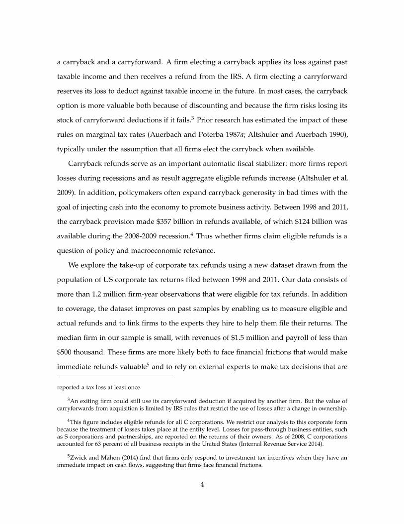
a carryback and a carryforward. A firm electing a carryback applies its loss against past

taxable income and then receives a refund from the IRS. A firm electing a carryforward

reserves its loss to deduct against taxable income in the future. In most cases, the carryback

option is more valuable both because of discounting and because the firm risks losing its

stock of carryforward deductions if it fails.3 Prior research has estimated the impact of these

rules on marginal tax rates (Auerbach and Poterba 1987a; Altshuler and Auerbach 1990),

typically under the assumption that all firms elect the carryback when available.

Carryback refunds serve as an important automatic fiscal stabilizer: more firms report

losses during recessions and as result aggregate eligible refunds increase (Altshuler et al.

2009). In addition, policymakers often expand carryback generosity in bad times with the

goal of injecting cash into the economy to promote business activity. Between 1998 and 2011,

the carryback provision made $357 billion in refunds available, of which $124 billion was

available during the 2008-2009 recession.4 Thus whether firms claim eligible refunds is a

question of policy and macroeconomic relevance.

We explore the take-up of corporate tax refunds using a new dataset drawn from the

population of US corporate tax returns filed between 1998 and 2011. Our data consists of

more than 1.2 million firm-year observations that were eligible for tax refunds. In addition

to coverage, the dataset improves on past samples by enabling us to measure eligible and

actual refunds and to link firms to the experts they hire to help them file their returns. The

median firm in our sample is small, with revenues of $1.5 million and payroll of less than

$500 thousand. These firms are more likely both to face financial frictions that would make

immediate refunds valuable5 and to rely on external experts to make tax decisions that are

reported a tax loss at least once.

3An exiting firm could still use its carryforward deduction if acquired by another firm. But the value ofcarryforwards from acquisition is limited by IRS rules that restrict the use of losses after a change in ownership.

4This figure includes eligible refunds for all C corporations. We restrict our analysis to this corporate formbecause the treatment of losses takes place at the entity level. Losses for pass-through business entities, suchas S corporations and partnerships, are reported on the returns of their owners. As of 2008, C corporationsaccounted for 63 percent of all business receipts in the United States (Internal Revenue Service 2014).

5Zwick and Mahon (2014) find that firms only respond to investment tax incentives when they have animmediate impact on cash flows, suggesting that firms face financial frictions.

4

unrelated to their core business.

We present three empirical findings. First, take-up is surprisingly low. Only 37 percent

of eligible firms claim their refund. This finding holds even when we restrict our attention

to potential refunds that are large relative to a firm’s operating cash flows. Although larger

firms are more likely to claim a refund, the take-up rate only reaches fifty percent at the

90th percentile of firm size in our data. Just half of the potential aggregate refund amount

was claimed and distributed to eligible firms. Thus the low take-up rate substantially limits

the potential impact of this policy as fiscal stimulus.

Second, we find that a simple cost-benefit analysis of the carryback-carryforward trade-

off cannot explain the low take-up rate. Because the loss provision presents firms with

a simple binary choice and our dataset allows us to compute the ex post value of each

option, our setting provides a unique opportunity to learn whether firms optimize with

respect to the tax code. Most firms that fail to claim do not benefit from waiting and many

non-claimers forgo more than thirty percent of the refund’s value. This finding is based on

firms for whom we can precisely compute the ex post net present value of the carryback

and carryforward options using each firm’s realized path of taxable income over time. In

our calculations, we assume discount rates ranging from three to nine percent. If firms

face financial frictions that generate higher discount rates, the net present value differences

between the carryback and the carryforward options would be even greater.

These findings suggest that either informational frictions or transaction costs prevent

firms from claiming their refunds. We consider these alternatives while exploring the

connection between tax preparers and client claiming behavior. By reducing informational

frictions and the cost of electing the carryback, preparers could play an important role

in determining client take-up. We evaluate this hypothesis by testing whether preparer

characteristics can account for the variation in corporate claiming behavior. The exercise

is similar to the approaches used to explore whether managerial “style” affects corporate

decisions (Bertrand and Schoar 2003; Kaplan, Klebanov and Sorensen 2012) and whether

teachers affect student test scores (Jackson and Bruegmann 2009). In addition to providing

5

insight into the take-up puzzle, this test also speaks to whether hired experts help firms

optimize.6

Our third finding is that firms with sophisticated preparers, such as those licensed

as certified public accountants (CPAs), are more likely to claim the refund. We begin

with a specification that includes firm fixed effects, so that the coefficients on preparer

characteristics are identified from firms that switch preparers while holding constant time-

invariant client unobservables. Relative to preparers without a professional license, the

clients of CPAs are 6.8 percentage points more likely to claim. This effect is large in

comparison to a baseline take-up rate of 37 percent. In addition to professional licenses,

other proxies for preparer sophistication—age, salary, client size, and client base size—also

coincide with higher take-up.

The research design relies on the identifying assumption that changes in preparers are

uncorrelated with unobservable changes in client determinants of take-up. Our estimates

will be biased if hiring a more sophisticated manager leads to hiring a more sophisticated

preparer and more sophisticated managers are more likely to claim refunds. We address

this threat in three ways. First, we confirm that our results are robust to a variety of client

control sets. Second, we confirm the absence of differential trends in claiming rates prior

to a preparer switch. Third, we validate our estimates in a sample of switching events in

which the prior preparer either dies or moves personal residence. Here it is more plausible

that around the event client unobservables do not change. We find similar estimates as in

our original design, indicating that selection does not confound our results.

Taken together, these facts reject the null that tax preparers do not influence the transmis-

sion of this policy. We attempt to quantify the relative impact of preparers using a simple

variance decomposition. Our estimate comes from the within-firm covariance structure for

observations that do and do not share the same preparer at different points in time. This

decomposition relies on a strong assumption of independence between the unobserved

6A growing literature documents the impact of managers on firm performance. Key contributions includeBertrand and Schoar (2003), Bloom and Van Reenen (2007), Kaplan, Klebanov and Sorensen (2012), and Bloomet al. (2013).

6

preparer effect and the unobserved firm error term. Based on this approach, we find that

the variance of the preparer effect equals 9 percent of the total variation in take-up. As a

benchmark for this magnitude, the prediction from firm observables accounts for 9 percent

of the variation in take-up. If selection into preparers does not affect take-up, preparers

matter as much as firm observables for predicting claiming behavior.

Our paper sits at the intersection of several strands in the economics, finance, and

accounting literatures. The literature on optimization frictions and behavioral responses to

tax policy mostly focuses on individual taxes and settings where imperfect information or

search costs affect responses to tax incentives.7 The literature on public program take-up

surveyed by Moffit (2003) and Currie (2006) has traditionally focused on social welfare

programs targeted at low-income and vulnerable populations. Many studies in this area

argue that these programs have low participation rates because of filing requirements and

poor information.8 We show that similar considerations apply to firms and demonstrate

that their claiming decisions depend on the third party experts they hire to help them. Our

results reject the standard view that firms optimize perfectly with respect to taxes.

The paper extends past research about the tax treatment of corporate losses.9 These

studies focus on how loss rules affect marginal incentives to invest and borrow. While they

emphasize that marginal tax rates do not equal statutory tax rates once firms take into

account the ability to offset gains in one year with losses in another, these papers typically

assume that firms always claim the carryback when available. Our results raise questions

about whether many firms take dynamic corporate tax incentives into account.

The paper also relates to a growing literature on the role of human capital in firm decision

7Key empirical studies include Chetty, Looney and Kroft (2009), Finkelstein (2009), Chetty et al. (2011),Chetty (2012), Chetty and Saez (2013), Chetty, Friedman and Saez (2013), and Goldin and Homonoff (2013).These papers have found evidence that individuals under-respond to taxes in the context of sales taxes, highwaytolls, and the individual income tax.

8Daponte and Taylor (1999), Currie and Grogger (2001), Bitler, Currie and Scholz (2003), Heckman andSmith (2004), and Aizer (2007) make this point in the context of food stamps, job training programs, and publichealth insurance.

9Key papers include Auerbach and Poterba (1987a), Altshuler and Auerbach (1990), Graham (1996), andGraham and Mills (2008).

7

making. These studies have documented that firm investment, leverage, and effective tax

rates depends on managerial style.10 In recent work, Klassen, Lisowsky and Mescall (2012)

find a cross-sectional relationship between the aggressiveness of corporate tax positions and

whether a firm’s financial auditor prepares the tax return. We introduce a novel research

design using quasi-experimental preparer switches based on deaths and relocations to show

that, in addition to internal managers, external consultants can significantly affect how firms

make decisions.

The paper proceeds as follows. Section 1.2 introduces the tax code’s loss rules, describes

the corporate tax data and sample selection process, and documents refund take-up among

eligible firms. Section 1.3 performs a cost-benefit assessment of the tax loss choice and shows

that the low take-up puzzle survives this analysis. Motivated by these findings, Section 1.4

describes the corporate market for tax preparation services and explores the relationship

between paid preparers and their clients’ claiming patterns. Section 2.6 discusses policy

implications and future research directions.

1.2 Corporate Losses and Tax Refunds

1.2.1 The Tax Code’s Loss Rules

Consider a firm that reports a tax loss. The corporate tax code allows the firm to apply

losses in one year to offset profits in other years and thus reduce its average tax burden. In

general, the firm can choose either to carry the loss back against past taxable income or

to carry the loss forward into the future. In tax code terminology, the option is between a

carryback and a carryforward.

The tax loss choice has economic consequences for the firm because the two options

differ in the timing of the tax benefit. Under the carryback, firms immediately receive a

10Bertrand and Schoar (2003) study the role of managers in corporate decision making. Bloom andVan Reenen (2007) and Kaplan, Klebanov and Sorensen (2012) document strong correlations between manage-ment practices and firm performance measures. Dyreng, Hanlon and Maydew (2010) and Armstrong, Blouinand Larcker (2012) show that managers influence corporate effective tax rates.

8

Table 1.1: Legislative background on tax loss carrybacks and carryforwards, 1998-2011

Ending fiscal period Carryback Carryforward(year-month)a period period Enacting legislation1998-12 to 2000-12 2 years 20 years TRA 1997 (permanent)c

2001-01 to 2002-12 5 years 20 years JCWAA 2002 (temporary)d

2003-01 to 2007-12 2 years 20 years TRA 1997 (permanent)2008-01 to 2010-11 5 years 20 years ARRA 2009 (temporary)b,e

WHBAA 2009 (temporary)b,f

2010-12 to 2012-11 2 years 20 years TRA 1997 (permanent)

Notes: This table summarizes the statutory window for eligible carrybacks and carryforwards between 1998and 2011. The policy rules apply to corporate tax returns with ending fiscal periods that fall within the rangedetailed in the first column of the table. The last column lists the legislation that enacted the policy changes. Inthis period, the carryback window was twice expanded temporarily as part of fiscal stimulus legislation. Theinformation for this table was pulled from bulletins and revenue procedures released by the Internal RevenueService.

a. Corporations file income taxes for the fiscal year instead of the calendar yearb. ARRA 2009 and WHBAA 2009 limited deductions against the fifth fiscal year preceding a firm’s currenttax loss to 50 percent of taxable incomec. TRA: Taxpayer Relief Act of 1997d. JCWAA: Job Creation and Worker Assistance Act of 2002e. ARRA: American Recovery and Reinvestment Act of 2009f. WHBAA: Worker, Homeowner, and Business Assistance Act of 2009

refund for the taxes they paid in the past. Under the carryforward, firms defer the tax

benefit to future periods when they deduct their loss against future taxable income. The

carryback is typically more valuable because the firm gets cash now, but the carryforward

can be better if the firm expects to pay a higher marginal tax rate in the future.

A statutory window limits the application of loss deductions to past and future tax

years. Table 1.1 summarizes the statutory window for carrybacks and carryforwards in

the US tax code over the 1998-2011 period. The carryback window was typically two years

during this time, except when Congress twice lengthened it to five years in response to

recessions. These policy changes enhanced the automatic stabilizer feature of the carryback

provision, which generates more refunds in bad times when corporate losses are common.

The carryforward window was twenty years throughout this same period.

The size of the refund generated by the carryback election depends on how much the

9

firm has paid in past taxes. When a firm claims the carryback, it must fully apply the loss to

all eligible past income. Loss firms are not eligible for a carryback refund when they do not

have any past income within the statutory window. In cases where the current loss exceeds

eligible past taxable income, a carryback election generates both a tax refund for past taxes

paid and a carryforward deduction equal to the losses in excess of past income.

To claim a carryback, the firm must file a special form to document how it computed its

carryback refund. The form details how the loss deduction is applied to past tax returns to

generate a tax refund.11 Upon approving the firm’s claim, the tax authority sends a refund

check equal to the amount of overpaid taxes in past years after taking into account the loss

deduction. To claim a carryforward, the firm must keep a record of its carryforward stock

from past losses and then take a net operating loss deduction on its future tax return. All

loss deductions against past and future taxable income are computed in nominal terms.

1.2.2 Business Tax Data

We use administrative IRS databases to document the impact of preparers on the claiming

of the carryback refund. This database includes all corporations that file a tax return in

the United States, approximately 6.5 million per year. We rely on two main files: a tax

return file that records line items from corporate income tax returns12 and a transactions file

that records debits and credits to individual tax liability accounts. We measure corporate

characteristics13 from the tax return file and claimed refunds from the transactions file.

We limit our study to C corporations because they are taxed at the firm level and retain

the decision over whether to claim the tax refund for losses. We exclude firms with mean

revenue and mean payroll measures less than $100,000 because they may not represent

11A firm claims the carryback by filing either Form 1139 or Form 1120X. To remain eligible for the carryback,the firm must file within three years of the due date (plus extensions) of the tax return where it reports the loss.Alternatively, the firm can elect to irrevocably forgo the carryback and fully carry forward the loss when it filesits income tax return. This election is made by checking a box on its income tax return.

12Form 1120 and Form 1120S.

13Corporate characteristics include revenue, assets, payroll, industry codes, and tax losses.

10

operating firms (Knittel et al. 2011). And to focus on firms with a meaningful carryback

option, our sample only includes firm-year observations that are eligible for a carryback

refund of at least $1,000.

Table 1.2 reports summary statistics for our sample. It consists of 1.24 million firm-year

observations and 612,070 individual firms. The median firm is small, with $1.5 million in

revenue, $489 thousand in assets, and $469 thousand in payroll. The eligible carryback

refunds are also moderate in size, with a median that equals almost $5.7 thousand. To

benchmark this amount, we compute the ratio of refund to revenue and the ratio of EBITDA

to revenue. The median for each quantity equals 0.4 percent and 4.6 percent respectively.

Compared to each other, they imply that the eligible refunds are a moderate share of

earnings.14

Table 1.2 also includes variables for the preparer and the tax firm matched to each

corporate tax return. Most corporations hire small tax firms. The median corporation hires

a tax firm with $0.8 million in revenue and 98 corporate clients. In cases where a preparer

or a tax firm cannot be matched to the corporate tax return, most typically the corporation

does not report using a third-party preparer.

Table 1.3 reports summary statistics for a subset of firms that switch preparers between

1998 and 2011. All observations in this subsample match to a preparer. This subsample only

includes two observations per firm: the last observation before switching preparers and the

first observation after switching preparers. It consists of 124,862 firm-year observations and

62,431 individual firms. Similar to the overall sample, the median firm is small with $1.9

million in revenue. The table also includes the preparer characteristics used to test whether

client claiming behavior depends on which preparer is employed.

We simulate each firm’s eligible carryback refund because the administrative IRS data

does not explicitly record this amount. Our algorithm first imputes each firm’s past taxable

income from its historical tax liability. We next use the policy rules to determine the eligible

14We do not report the ratio of refunds to EBITDA directly because EBITDA is often negative.

11

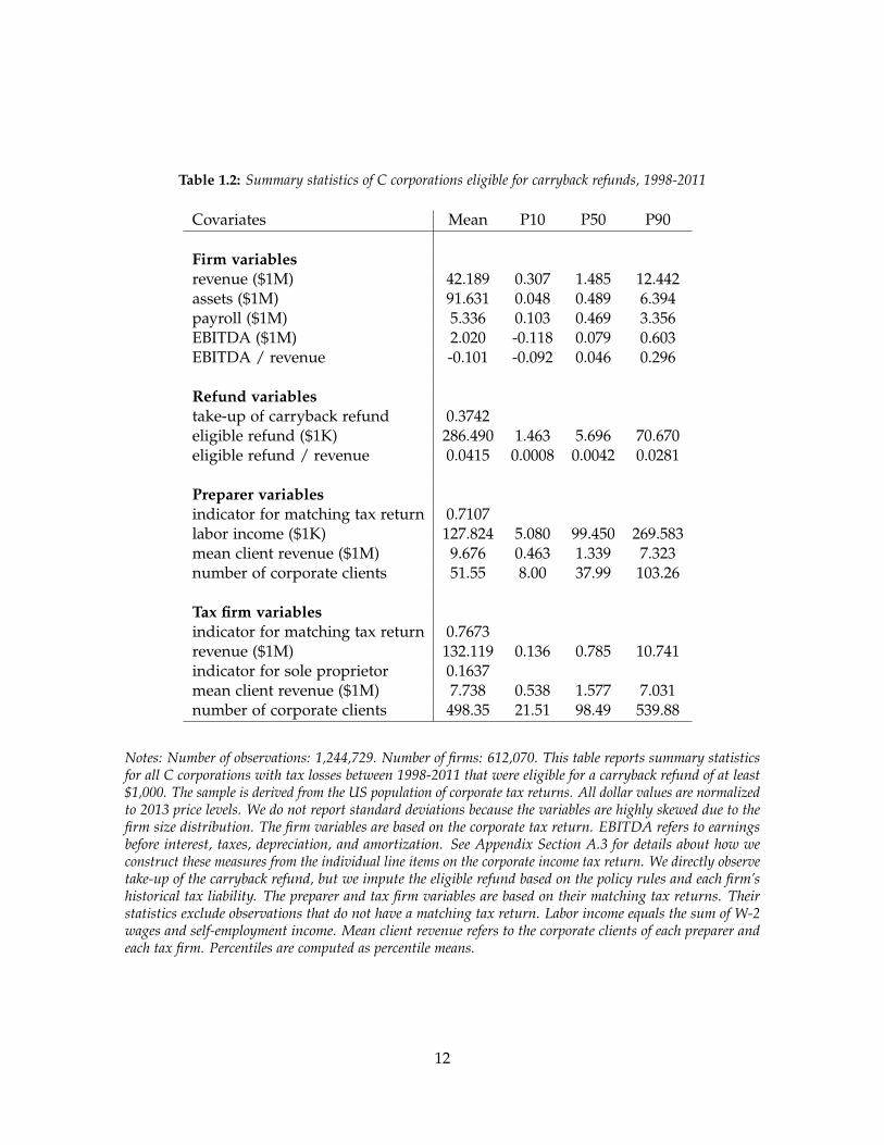
Table 1.2: Summary statistics of C corporations eligible for carryback refunds, 1998-2011

Covariates Mean P10 P50 P90

Firm variablesrevenue ($1M) 42.189 0.307 1.485 12.442assets ($1M) 91.631 0.048 0.489 6.394payroll ($1M) 5.336 0.103 0.469 3.356EBITDA ($1M) 2.020 -0.118 0.079 0.603EBITDA / revenue -0.101 -0.092 0.046 0.296

Refund variablestake-up of carryback refund 0.3742eligible refund ($1K) 286.490 1.463 5.696 70.670eligible refund / revenue 0.0415 0.0008 0.0042 0.0281

Preparer variablesindicator for matching tax return 0.7107labor income ($1K) 127.824 5.080 99.450 269.583mean client revenue ($1M) 9.676 0.463 1.339 7.323number of corporate clients 51.55 8.00 37.99 103.26

Tax firm variablesindicator for matching tax return 0.7673revenue ($1M) 132.119 0.136 0.785 10.741indicator for sole proprietor 0.1637mean client revenue ($1M) 7.738 0.538 1.577 7.031number of corporate clients 498.35 21.51 98.49 539.88

Notes: Number of observations: 1,244,729. Number of firms: 612,070. This table reports summary statisticsfor all C corporations with tax losses between 1998-2011 that were eligible for a carryback refund of at least$1,000. The sample is derived from the US population of corporate tax returns. All dollar values are normalizedto 2013 price levels. We do not report standard deviations because the variables are highly skewed due to thefirm size distribution. The firm variables are based on the corporate tax return. EBITDA refers to earningsbefore interest, taxes, depreciation, and amortization. See Appendix Section A.3 for details about how weconstruct these measures from the individual line items on the corporate income tax return. We directly observetake-up of the carryback refund, but we impute the eligible refund based on the policy rules and each firm’shistorical tax liability. The preparer and tax firm variables are based on their matching tax returns. Theirstatistics exclude observations that do not have a matching tax return. Labor income equals the sum of W-2wages and self-employment income. Mean client revenue refers to the corporate clients of each preparer andeach tax firm. Percentiles are computed as percentile means.

12

Table 1.3: Summary statistics of C corporations that change preparers, 1998-2011

StandardCovariates Mean deviation P10 P50 P90

Firm variablesrevenue ($1M) 24.877 0.338 1.873 23.370assets ($1M) 38.817 0.063 0.650 15.285payroll ($1M) 5.027 0.103 0.572 5.801EBITDA ($1M) 0.525 -0.228 0.075 0.796EBITDA / revenue -0.149 -0.109 0.037 0.264

Refund variablestake-up of carryback refund 0.3572eligible refund ($1K) 233.866 1.566 7.045 125.411eligible refund / revenue 0.0506 0.0007 0.0042 0.0298

Preparer variablesI(certified public accountant) 0.8314I(attorney) 0.0214I(other professional license) 0.0556log(labor income) 11.36 1.17 9.98 11.57 12.51I(self-employment) 0.1794age 49.89 11.17 35.52 50.00 63.48log(mean client revenue) 14.59 1.50 13.06 14.27 16.62log(total client revenue) 17.86 1.82 15.50 17.94 20.11

Notes: Number of observations: 124,862. Number of firms: 62,431. This table reports summary statistics forthe sample of C-corporations that were eligible for carryback refunds of at least $1,000, that switched preparersbetween 1998 and 2011, and that reported preparer identifiers which match to a tax return. All dollar valuesare normalized to 2013 price levels. We do not report standard deviations for the firm and refund variablesbecause they are highly skewed due to the firm size distribution. The firm variables are based on the corporatetax return. EBITDA refers to earnings before interest, taxes, depreciation, and amortization. See AppendixSection A.3 for details about how we construct these measures from the individual line items on the corporateincome tax return. We directly observe take-up of the carryback refund, but we impute the eligible refund basedon the policy rules and each firm’s historical tax liability. The preparer variables are based on their matchingtax returns. Labor income equals the sum of W-2 wages and self-employment income. The self-employmentindicator reflects preparers that derive at least half of their labor income from self-employment. Mean and totalclient revenue refer to the corporate clients of the individual preparers. Percentiles are computed as percentilemeans.

13

carryback window. Starting with the earliest eligible year, we deduct the current tax loss15

against imputed past taxable income. We continue with these deductions until either the

current loss or past taxable income is exhausted. We then re-computes the historical tax

liability based on the post-deduction taxable income. The difference between the pre-

deduction and post-deduction tax liability equals our simulation for the eligible carryback

refund.

We verify our algorithm for the eligible refunds using firms that claim the carryback.

Although the IRS database does not track the eligible refunds, it does record the claimed

amounts. For the subset of firms that make the carryback election, we can directly compare

the claimed amount to the simulated amount. Our results indicate that we impute the

eligible refunds with a high degree of accuracy. When we regress log(claimed amount) on

log(eligible amount), we find a coefficient of 0.9636 and an R2 of 0.9336. Appendix Section

A.1 describes in more detail how we construct and validate our measure for the eligible

refund.

1.2.3 Low Take-up of Tax Refunds for Losses

Eligibility for the carryback refund is common. Figure 1.1 reports the annual share of loss

firms from the population of C corporations. It also reports the share of firms eligible for

a carryback refund of at least $1,000. Over the 1998-2011 period, 37 percent of firm-year

observations report tax losses and 80 percent of firms report a loss at least once. Among tax

loss firms, 28 percent are eligible for a carryback refund. Firms frequently face the choice

between whether to apply their tax loss deduction as a carryback or a carryforward.

In addition, the aggregate magnitude of the carryback refunds is macroeconomically

relevant. Figure 1.2 reports the annual amount of eligible and claimed refunds for the

population of C corporations. Over the 1998-2011 period, C corporations claimed $187

15Tax losses are defined from the front page of the income tax return for C corporations. We use the statutorydefinition of tax losses for ordinary income. It equals net income (Line 28) + special deductions (Line 29b). Thisdefinition excludes capital income losses. It also excludes losses obtained from mergers and acquisitions, whichare reported with the stock of losses from prior periods (Schedule K, Line 12).

14

Figure 1.1: Frequency of tax losses and carryback refunds

1998 2000 2002 2004 2006 2008 2010

0.0

0.1

0.2

0.3

0.4

0.5

0.6

tax year

shar

e of

pop

ulat

ion

of C

−co

rpor

atio

ns

● ●

●

●

●

●

●●

●

●

●●

●●

●

firms that report a tax lossfirms eligible for carryback refundfirms that claim carryback refund

Notes: This figure plots the share of C corporations that report a tax loss, that are eligible for a carryback refund,and that claim the carryback refund. It is based on the population of corporate tax returns for C corporations.We limit eligibility to firms that have the option to claim a carryback refund of at least $1,000. We excludefirms with mean revenue and mean payroll less than $100,000 because they may not represent real operatingentities.

15

billion. Carryback refunds play an even larger role as countercyclical policy, totaling $68

billion in 2008 and 2009. As a benchmark, payments for unemployment insurance equaled

$209 billion during these years (US Department of Labor 2014).

Claimed refund amounts, however, significantly understate the potential size of the

policy. Only 37 percent of eligible firms claimed their refund. In aggregate, eligible refunds

are nearly twice as large as claimed refunds. During the 1998-2011 period, C corporations

were eligible for $357 billion in carryback refunds. In 2008 and 2009 alone, they were eligible

for $124 billion. Thus low take-up substantially undermines the potential effect of the

carryback refund as fiscal stimulus.

1.3 Evidence on Tax Loss Choices

In this section, we implement a cost-benefit analysis on the set of eligible firms to compare

the net present value of the carryback and carryforward options. This setting provides a

rare opportunity to evaluate whether firms make the value-maximizing choice. Despite the

low take-up rate, 79 percent of firms value the carryback more than the carryforward. We

discuss alternative reasons for the low take-up rates.

1.3.1 A Cost-Benefit Analysis of Tax Loss Choices

Loss firms deciding between the carryback and the carryforward elections need to consider

whether it would be more valuable to use the loss as a deduction against past taxable

income or against future taxable income. The value of the carryback depends on the tax

rates that the firm paid in the past. In contrast, the carryforward value depends on the tax

rates that it will pay in the future, the length of time that it will take the firm to return to

a profitable state, and the firm’s discount rate. These considerations also arise when the

corporate loss exceeds eligible past taxable income because the carryback election generates

a carryforward deduction equal to the loss in excess of eligible past income.

Computing the value of the carryback and carryforward elections involves a net present

value calculation because either option can generate carryforward deductions to be applied

16

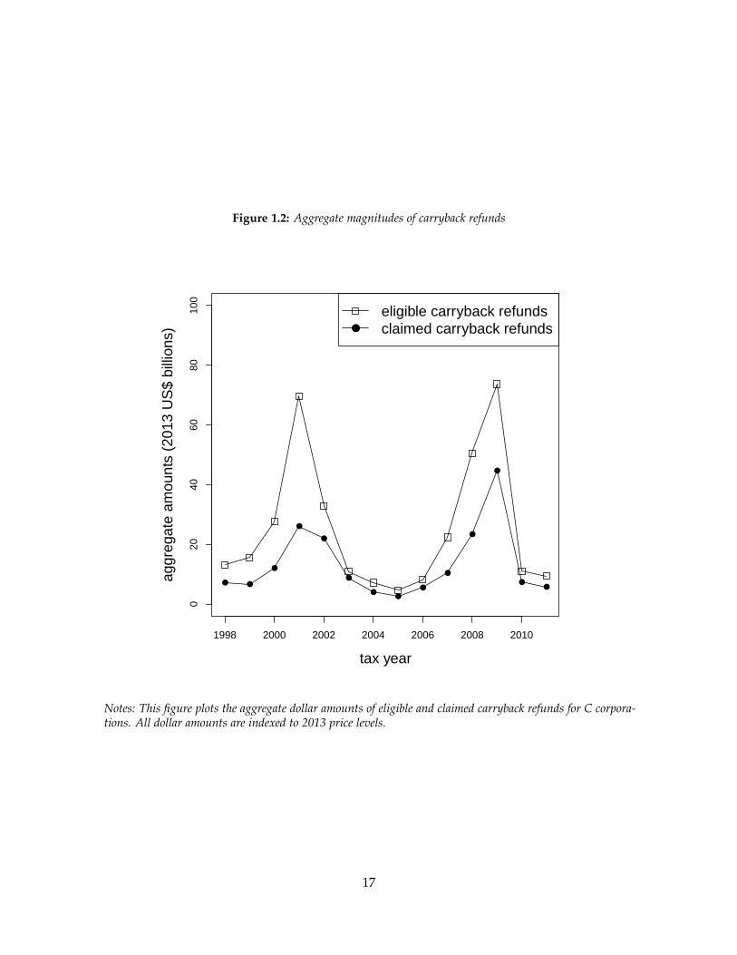
Figure 1.2: Aggregate magnitudes of carryback refunds

1998 2000 2002 2004 2006 2008 2010

020

4060

8010

0

tax year

aggr

egat

e am

ount

s (2

013

US

$ bi

llion

s)

● ●

●

●

●

●

●●

●

●

●

●

●●

●

eligible carryback refundsclaimed carryback refunds

Notes: This figure plots the aggregate dollar amounts of eligible and claimed carryback refunds for C corpora-tions. All dollar amounts are indexed to 2013 price levels.

17

against future taxable income. The key difference between their formulas is that the

carryback election deducts the loss against past taxable income and the carryforward

election does not. Carryback deductions against past taxable income are not discounted

because they generate an immediate tax refund.

We formalize the net present value formulas for the carryback and carryforward elections

under the assumption that the firm has perfect foresight over the timing of future taxable

income,

NPVb =−1∑

t=Tmin

τt Dbt +

Tmax

∑t=1

τt Dbt

(1+r)t

NPV f =Tmax

∑t=1

τt D ft

(1+r)t

(1.1)

where τt is the tax rate in time t, Dbt is the deduction taken in time t under the carryback

election, D ft is the deduction taken in time t under the carryforward election, and r is the

firm’s discount rate for future tax savings. Time is indexed relative to the loss at time

t = 0. Deductions applied to past taxable income are not discounted because the refund

is immediate. In either case, the nominal sum of the deductions cannot exceed the loss

reported at time t = 0. The nominal sum of the deductions can be less than the current loss

in cases where the firm does not have sufficient past and future taxable income to offset the

loss.

Table 1.4 uses a numerical example to clarify the differences between the carryback and

carryforward elections. For a firm with a loss of $100, we compute how deductions under

the carryback and carryforward elections would be applied to the firm’s taxable income.

Under the carryback election, the firm first deducts its loss against taxable income in period

t = −2. It deducts its remaining loss against taxable income in period t = −1. Assuming a

tax rate of 35 percent, the net present value of the carryback election equals $100× τ = $35.

Under the carryforward election, the firm deducts all of its loss against taxable income

in period t = 2. Assuming a tax rate of 35 percent and a discount rate of 7 percent, the

net present value of the carryforward election equals 100×τ(1+r)2 = $30.57. In this example, the

carryback election has a higher net present value because the tax rate is constant over time

and the firm discounts future tax savings.

18

Table 1.4: Example of loss deduction under carryback and carryforward elections

Event time relative to loss year-2 -1 0 1 2 3

Taxable income before loss deduction 50 100 -100 0 100 100

Panel A: carryback electionLoss deduction -50 -50 +100 0 0 0Taxable income after loss deduction 0 50 0 0 100 100NPV of carryback election 100 τ = $35

Panel B: carryforward electionLoss deduction 0 0 +100 0 -100 0Taxable income after loss deduction 50 100 0 0 0 100NPV of carryback election 100 τ

(1+r)2 = $30.57

Notes: This table illustrates the application of carryback and carryforward deductions for a firm that reports atax loss of $100 at time t = 0. Panel A assumes that the firm makes the carryback election and Panel B assumesthat the firm makes the carryforward election. The illustration also assumes that the firm pays a tax rate ofτ = 0.35 and has a discount rate of r = 0.07. Under the carryback election in Panel A, the hypothetical firmapplies its loss deduction against its past taxable income. It starts with the earliest eligible tax year (t = −2)and then proceeds to the next tax year (t = −1). Under the carryforward election in Panel B, the hypotheticalfirm applies its loss deduction against its future taxable income. In this example, we assume that the firmclaims the loss deduction as early as possible (t = 2). Even though this hypothetical firm always pays the sametax rate, the net present value of these two elections differ because they realize the tax benefits at different times.The carryback election realizes the tax benefits immediately at time t = 0 as a tax refund. In contrast, thecarryforward election defers the tax benefits until time t = 2 when it claims its loss deduction. In this example,the carryback election has a higher net present value than the carryforward election because it realizes its taxbenefit earlier.

19

1.3.2 Empirical Evaluation of Cost-Benefit Formulas

We empirically evaluate the net present value formulas in Equation 1.1 for firms with losses

between 1998 and 2002. We restrict our sample to this period because we want to use a

future 10-year period of realized taxable income to value each firm’s carryforwards. We

assume that all firms in this period do not have any carryforwards from prior tax years.

We make this assumption because the administrative tax data does not begin to collect this

information until 2003. We find similar results when we replicate our analysis on firms with

losses in 2003 where we do not need make assumptions about their pre-existing stock of

carryforwards. We also limit our sample to firms with eligible refunds of at least $1,000 to

exclude firms that do not have a meaningful carryback option.

We simulate the claiming of future carryforward deductions over a 10-year period based

on their realized taxable income. We perform this simulation under both the carryback

and carryforward elections. We assume that firms will claim their future carryforward

deductions as soon as possible and, in cases of surviving firms that have unused losses

after 10 years, that all unused losses are claimed in the 11th year. We then compute the net

present values of the carryback and carryforward elections assuming a discount rate of 7

percent.

We calculate the net present value difference between the carryback and carryforward

elections, NPVb − NPV f , and plot its histogram in Figure 1.3. For 79 percent of the sample,

the carryback election has a larger net present value than the carryforward election. This

difference is greater than $844 for half the sample.16 Based on this simple net present value

comparison, the majority of firms value the carryback more than the carryforward election.

This finding is robust to our assumption of a 7 percent discount rate. In Table 1.5, we

show the sensitivity of our results to the assumed discount rate. For a given threshold and

discount rate, the table reports the share of firms where the ratio of NPV f to NPVb is less

than the threshold. Each column assumes a different threshold and each row assumes a

16These results are robust to constructing an ex ante measure of net present value based on forecasting theex post net present value in a linear regression with firm covariates.

20

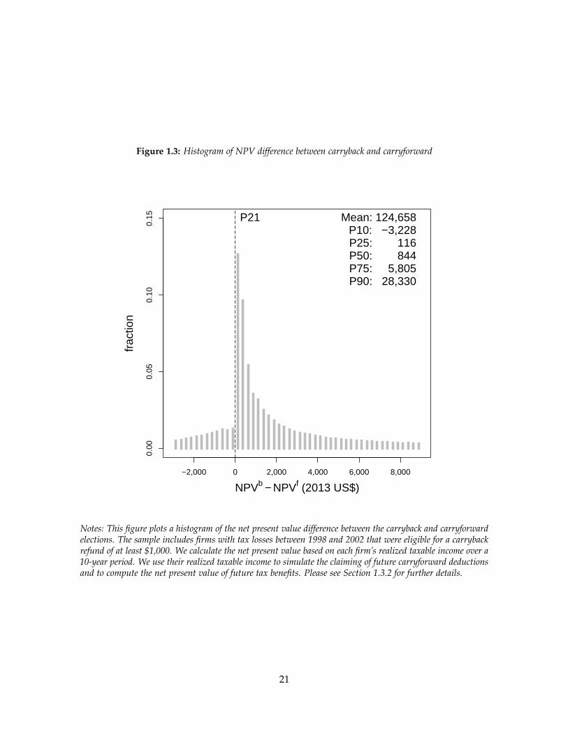
Figure 1.3: Histogram of NPV difference between carryback and carryforward0.

000.

050.

100.

15

NPVb − NPVf (2013 US$)

frac

tion

−2,000 0 2,000 4,000 6,000 8,000

P21 Mean: 124,658P10: −3,228P25: 116P50: 844P75: 5,805P90: 28,330

Notes: This figure plots a histogram of the net present value difference between the carryback and carryforwardelections. The sample includes firms with tax losses between 1998 and 2002 that were eligible for a carrybackrefund of at least $1,000. We calculate the net present value based on each firm’s realized taxable income over a10-year period. We use their realized taxable income to simulate the claiming of future carryforward deductionsand to compute the net present value of future tax benefits. Please see Section 1.3.2 for further details.

21

Table 1.5: Share of firms below alternative thresholds for NPVf /NPVb

Firm Maximum value for NPVf /NPVbdiscount rate 1 0.9 0.8 0.7

3% 0.7499 0.4163 0.3246 0.28285% 0.7719 0.4955 0.3634 0.30017% 0.7911 0.5727 0.4109 0.32619% 0.8087 0.6127 0.4644 0.3574

Notes: This table compares the net present value of the carryforward and carryback elections for firms withtax losses between 1998 and 2002. It shows the sensitivity of our results to the assumed firm discount rate.The table reports the share of firms for whom the ratio of the carryforward net present value to the carrybacknet present value is below a maximum threshold. Each column assumes a different maximum threshold andeach row assumes a different firm discount rate for the net present value calculation. The sample only includesfirms that were eligible for a carryback refund of at least $1,000. NPVf indicates the net present value for thecarryforward election. NPVb indicates the net present value of the carryback election. Please see Section 1.3.2for further details.

different discount rate. Varying the discount rate between 3 and 9 percent, the share of

firms where the net present value of the carryback election is greater than the carryforward

election ranges between 75 and 81 percent.

Figure 1.4 compares the net present value difference between the carryback and the

carryforward options to an estimate of the labor cost for submitting a carryback application.

It provides a benchmark for evaluating the magnitude of the net present value difference.

Anecdotal conversations with preparers that serve firms in the size range of our sample

suggest that filing for the carryback involves one to two hours of additional work. Figure

1.4 plots the imputed hourly wage of preparers at the 25th, 50th, and 75th percentiles by

the net present value difference between the carryback and the carryforward options. We

impute the hourly wage by dividing each individual preparer’s annual labor income17 by

40× 50 = 2000. This denominator assumes that preparers work 40 hours each week for 50

weeks over the course of a year.

We find that the imputed hourly wage remains relatively constant regardless of the net

present value difference. The imputed wage equals approximately $20, $45, and $80 at the

17We define labor income as the sum of W-2 earnings and self-employment income.

22

Figure 1.4: Imputed preparer wage by NPV difference between carryback and carryforward0

2040

6080

100

120

NPVb − NPVf (2013 US$)

impu

ted

hour

ly w

age

of p

repa

rer

(201

3 U

S$)

●

●●

● ● ●●

● ● ● ●● ● ● ● ● ● ● ● ●

●

●

● ● ●●

● ●● ●

●● ● ●

● ●● ●

● ● ●

●

●●

● ● ●●

−2,000 0 2,000 4,000 6,000 8,000

●

75th percentile50th percentile25th percentile

Notes: This figure plots the 25th, 50th, and 75th percentiles in imputed preparer wages by the net presentvalue difference between the carryback and the carryforward options. The sample includes firms with tax lossesbetween 1998 and 2002 that were eligible for a carryback refund of at least $1,000. Wages are imputed bydividing preparer labor income by 2000. This computation assumes that preparers bill 40 hours per week over50 weeks in one calendar year. Labor income equals the sum of W-2 earnings and self-employment income.Dollar amounts are normalized to 2013 price levels.

23

25th, 50th, and 75th percentiles. Even allowing for a mark-up for overhead expenses and

profit, the net present value differences between the carryback and the carryforward options

are large relative to these estimates of the labor costs.18

Figure 1.5 provides an alternative benchmark for whether firms should make the car-

ryback or the carryforward election. It compares the observed growth rates in corporate

taxable income to hypothetical growth rates at which the net present value of the carryback

and carryforward options equal each other. The observed growth rates are computed using

each firm’s observed taxable income between the year of the net operating loss and the tenth

year after the loss. We find the growth rate with a linear fit that intersects the y-axis at the

value of the initial loss. The break-even growth rates are computed from a linear forecast

over a ten-year period following the loss year. The initial value for the linear forecast also

equals the firm’s net operating loss.

We present this comparison as a histogram of the ratio between the observed growth

rate and the break-even growth rate. The observed and break-even growth rates equal each

other when the ratio equals one. The ratio is less than one in cases where the observed

growth rate is less than the break-even growth rate. The ratio can be negative because some

firms experience negative growth rates in taxable income following their loss.

We find that the observed growth rate is less than the break-even rate in most cases. The

mean ratio of observed to break-even growth rates equals 0.26. The observed growth rate

is less than the break-even growth rate for 94 percent of observations. This result differs

from a comparison of the net present value of the carryback and the carryforward options

because, in this exercise, we assume a linear growth rate in taxable income (which smooths

the volatility). This comparison implies that few firms experience growth rates in taxable

income that would make electing the carryforward more valuable than the carryback option.

18In cases where a team of preparers file a tax return for a client, the head of the team will typically sign theclient’s return. Because our sample consists predominantly of small corporations that hire small tax firms, wesuspect that most client returns are prepared by individuals.

24

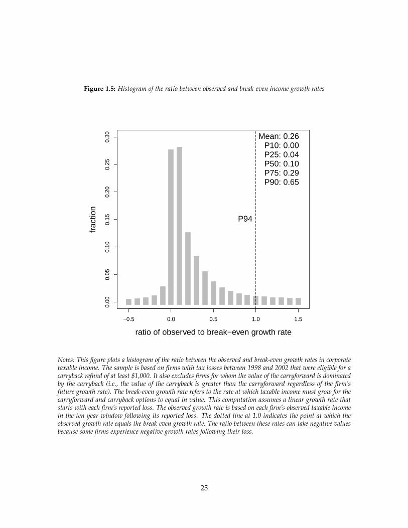
Figure 1.5: Histogram of the ratio between observed and break-even income growth rates

0.00

0.05

0.10

0.15

0.20

0.25

0.30

ratio of observed to break−even growth rate

frac

tion

−0.5 0.0 0.5 1.0 1.5

P94

Mean: 0.26P10: 0.00P25: 0.04P50: 0.10P75: 0.29P90: 0.65

Notes: This figure plots a histogram of the ratio between the observed and break-even growth rates in corporatetaxable income. The sample is based on firms with tax losses between 1998 and 2002 that were eligible for acarryback refund of at least $1,000. It also excludes firms for whom the value of the carryforward is dominatedby the carryback (i.e., the value of the carryback is greater than the carryforward regardless of the firm’sfuture growth rate). The break-even growth rate refers to the rate at which taxable income must grow for thecarryforward and carryback options to equal in value. This computation assumes a linear growth rate thatstarts with each firm’s reported loss. The observed growth rate is based on each firm’s observed taxable incomein the ten year window following its reported loss. The dotted line at 1.0 indicates the point at which theobserved growth rate equals the break-even growth rate. The ratio between these rates can take negative valuesbecause some firms experience negative growth rates following their loss.

25

1.3.3 Alternative Explanations for Low Take-Up

The results from our cost-benefit exercise make the the low take-up rate of the carryback

refund puzzling. Based on a net present value comparison alone, most firms should claim

the carryback. We next consider alternative rationales for why a minority of eligible firms

would claim the carryback.

First, small firms may not know how to file for the carryback refund, or even that

this option is available to them. Claiming it involves submitting an additional form and

recomputing the firm’s income tax for each prior tax year affected by the carryback. Small

firms without professional expertise regarding the tax code may find the filing requirements

to claim the carryback refund too complicated.

Second, a firm’s preparer may charge additional fees for claiming the carryback refund.

While the preparer may know how to claim it, filing for the carryback still involves additional

effort on their part. In this industry, it is common for preparers to bill their clients by the

hour or by the tax form. The additional fees for claiming the refund may be sufficient to

deter clients.

Third, firms may be concerned that filing for a carryback refund will put them at risk

for an IRS audit. When a firm applies for the carryback, an IRS employee must review

their recomputed tax liability for prior years. This carries the risk that the IRS will spot

something that will prompt an audit. Even if the actual risk is small, the perceived risk may

be sufficient to deter filing for the carryback claim.

Each of these alternative explanations creates opportunities for preparers to determine

whether their client claims the carryback refund. Firms hire preparers to inform them about

the tax code, file tax returns on their behalf, and warn them about the audit risk of different

tax reporting choices. Preparers may differ in whether they encourage their clients to claim

the tax refund based on their own beliefs about its merits for their clients, its filings costs,

and its audit risks.

26

1.4 Tax Preparers and the Take-up of Tax Refunds

In this section, we provide evidence that client take-up of the carryback refund depends

on preparers. We start with background information about the corporate market for

tax preparation services to provide context for our results. We then show that preparer

characteristics predict whether firms claim the carryback refund using a research design

based on firms that switch preparers. We also causally validate our results by focusing on

a subset of switching events where the prior preparer either dies or moves their personal

residence. In these cases, we find it more plausible that changes in client unobservables

do not confound our estimates. We conclude with an analysis of variance exercise that

finds that, if selection into preparers does not affect take-up, an unobserved preparer effect

accounts for as much of the variation in claiming behavior as firm observables.

1.4.1 Corporate Market for Tax Preparation Services

A large private market provides tax preparation services to firms. In 2012, 96 percent of cor-

porations hired an external preparer to file their income taxes. The market employs 188,735

individual preparers who file tax returns for corporations. Although federal regulations do

not mandate any licensing requirements for preparers, 89 percent of firms hired a preparer

with a professional license19 (predominantly certified public accountants). The remaining 10

percent of firms hired preparers without any professional credentials.20

The tax preparation market includes a wide variety of tax firms. They range from sole

proprietorships with a single employee to national brands with thousands of locations.

These firms also vary in their degree of specialization. Some focus on tax preparation

(e.g., H&R Block, Inc.) whereas others offer a broad portfolio of professional services for

businesses (e.g., BDO USA, LLP). Despite these differences, employees at most tax firms use

19Either a certified public accountant, attorney, enrolled agent, or state licensed preparer. Enrolled agents arelicensed by the Internal Revenue Service. They must pass an examination and fulfill 72 hours of continuingeducation every three years.

20Based on corporate preparers for the 2012 tax year.

27

a tax preparation software to service their clients (Internal Revenue Service 2009).

1.4.2 Claiming Decisions and Preparer Characteristics

Baseline Specification. We use firms that switch preparers to show that preparer charac-

teristics predict claiming behavior. Our analysis uses a sample of firms that were eligible

for carryback refunds of at least $1,000 between 1998 and 2011. We restrict the sample to

firms that were eligible in multiple years and that switched preparers. Because we want

to identify our result from variation due to changing preparers, we only include the last

observation before switching preparers and the first observation after switching preparers

for each firm in the sample. These observations are often not consecutive because firms are

not eligible for the carryback refund in each tax year. If a firm changes preparers multiple

times, we only include observations associated with the last switching event.

We estimate Equation 1.2 in a panel regression given by

I(carryback take-up)ijt = ZJ(i,t)γ + Xitβ + αi + δt + εit (1.2)

where the subscripts represent client i with preparer j in tax year t, ZJ(i,t) are preparer

characteristics, Xit are client characteristics, αi is the client fixed effect, and δt is the tax year

fixed effect. Preparer observables include indicators for professional credentials,21 log(labor

income), I(self-employment),22 age, log(mean client revenue), and log(total client revenue).

Client observables include log(revenue), log(assets), and log(EBITDA).

Our estimates of Equation 1.2 rely on the following identifying assumption:

Assumption 1 [Switchers Design]: The error term εit must satisfy the strict

exogeneity condition E[εit|ZJ(i,t), Xit, αi, δt] = 0.

This condition implies that client unobservables in the error term must be uncorrelated

21We include separate indicators for certified public accountants, attorneys, and preparers with anotherprofessional license. The last category includes enrolled agents and state licensed preparers. The omittedcategory are preparers without any professional credential.

22The self-employment indicator equals one if the preparer derives at least half of their labor income fromself-employment.

28

with preparer characteristics, client observables, a client fixed effect, and a tax year fixed

effect. Because the switchers design uses within-firm variation, this assumption will hold

if unobservable determinants of carryback take-up remain unchanged before and after

switching preparers.

We report estimates from the switchers design in Table 1.6. The regressions are univariate

with respect to preparer characteristics. All regressions include a firm fixed effect, a tax

year fixed effect, and firm controls. They also include dummies for missing values of the

preparer characteristics and the client controls. We block bootstrap the standard errors

by firm23 and report them in parentheses. With the exception of the category for “other

professional license”, all preparer covariates are statistically significant at the one percent

level.

We find that proxies for preparer sophistication predict claiming of the carryback refund.

Preparers that are certified public accountants, that are attorneys, that are better paid, that

do not work for themselves, that are older, and that have bigger client bases are more likely

to claim the carryback refund for their clients. Our results indicate that preparers matter for

client claiming behavior.

The professional certification categories and the client base measures have the coefficients

with the largest magnitudes. Relative to preparers without a professional license, certified

public accountants are 6.8 percentage points more likely to claim the carryback refund

for their clients. Similarly, attorneys are 4.7 percentage points more likely to claim. The

results also imply that a one standard deviation increase in log(mean client revenue) would

increase take-up by 2.7 percentage points. Likewise, a one standard deviation increase in

log(total client revenue) would increase take-up by 2.3 percentage points. These effects are

substantial relative to a baseline take-up rate of 37 percent in the population.

We test the sensitivity of our results to varying the set of controls and to including all

preparer characteristics in a multivariate regression. Table 1.7 reports these estimates. All

regressions include a firm fixed effect. Columns (2) and (5) add a tax year fixed effect.

23We bootstrap with 250 replications.

29

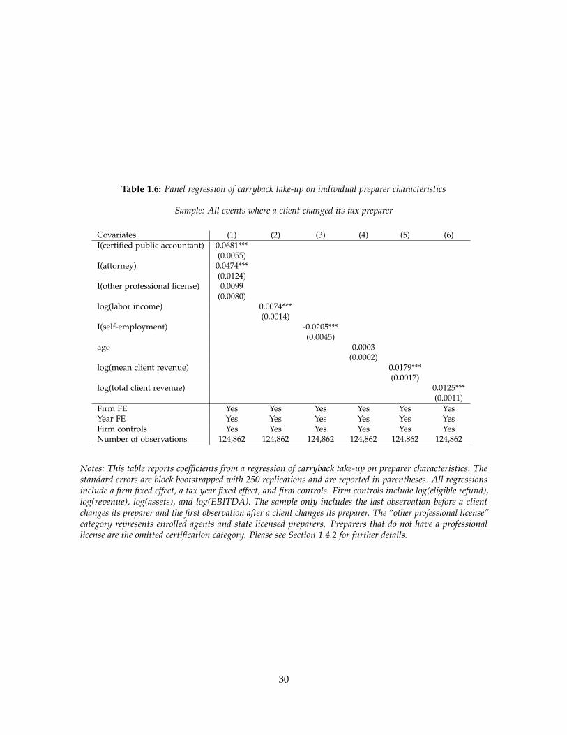
Table 1.6: Panel regression of carryback take-up on individual preparer characteristics

Sample: All events where a client changed its tax preparer

Covariates (1) (2) (3) (4) (5) (6)I(certified public accountant) 0.0681***

(0.0055)I(attorney) 0.0474***

(0.0124)I(other professional license) 0.0099

(0.0080)log(labor income) 0.0074***

(0.0014)I(self-employment) -0.0205***

(0.0045)age 0.0003

(0.0002)log(mean client revenue) 0.0179***

(0.0017)log(total client revenue) 0.0125***

(0.0011)Firm FE Yes Yes Yes Yes Yes YesYear FE Yes Yes Yes Yes Yes YesFirm controls Yes Yes Yes Yes Yes YesNumber of observations 124,862 124,862 124,862 124,862 124,862 124,862

Notes: This table reports coefficients from a regression of carryback take-up on preparer characteristics. Thestandard errors are block bootstrapped with 250 replications and are reported in parentheses. All regressionsinclude a firm fixed effect, a tax year fixed effect, and firm controls. Firm controls include log(eligible refund),log(revenue), log(assets), and log(EBITDA). The sample only includes the last observation before a clientchanges its preparer and the first observation after a client changes its preparer. The “other professional license”category represents enrolled agents and state licensed preparers. Preparers that do not have a professionallicense are the omitted certification category. Please see Section 1.4.2 for further details.

30

Table 1.7: Panel regression of carryback take-up on multiple preparer characteristics

Sample: All events where a client changed its tax preparer

Covariates (1) (2) (3) (4) (5) (6)I(certified public accountant) 0.0718*** 0.0725*** 0.0681*** 0.0605*** 0.0611*** 0.0590***

(0.0059) (0.0065) (0.0058) (0.0061) (0.0063) (0.0062)I(attorney) 0.0510*** 0.0496*** 0.0474*** 0.0404*** 0.0385*** 0.0387***

(0.0141) (0.0130) (0.0129) (0.0140) (0.0139) (0.0130)I(other professional license) 0.0049 0.0044 0.0099 0.0043 0.0043 0.0092

(0.0089) (0.0086) (0.0081) (0.0089) (0.0087) (0.0087)log(labor income) 0.0049*** 0.0047*** 0.0042***

(0.0016) (0.0016) (0.0015)I(self-employment) -0.0142*** -0.0140*** -0.0158***

(0.0049) (0.0047) (0.0046)age 0.0006*** 0.0007*** 0.0006***

(0.0002) (0.0001) (0.0001)log(mean client revenue) 0.0122*** 0.0136*** 0.0091***

(0.0024) (0.0026) (0.0024)log(total client revenue) 0.0066*** 0.0063*** 0.0057***

(0.0015) (0.0017) (0.0016)Firm FE Yes Yes Yes Yes Yes YesYear FE No Yes Yes No Yes YesFirm controls No No Yes No No YesNumber of observations 124,862 124,862 124,862 124,862 124,862 124,862

Notes: This table reports coefficients from a regression of carryback take-up on preparer characteristics. Thestandard errors are block bootstrapped with 250 replications and are reported in parentheses. All regressionsinclude a firm fixed effect. Columns (2) and (5) add a tax year fixed effect. Columns (3) and (6) add firmcontrols, which include log(eligible refund), log(revenue), log(assets), and log(EBITDA). The sample onlyincludes the last observation before a client changes its preparer and the first observation after a client changesits preparer. The “other professional license” category represents enrolled agents and state licensed preparers.Preparers that do not have a professional license are the omitted certification category. Please see Section 1.4.2for further details.

Columns (3) and (6) add firm controls. All regressions also include dummies for missing

values of the preparer characteristics and the client controls. The first three columns limit

the preparer characteristics to the professional license categories. The last three columns

include all preparer characteristics. We block bootstrap the standard errors by firm24 and

report them in parentheses.

The point estimates are not sensitive to the specification tests in Table 1.7. The magnitudes

slightly decrease with the expansion of the set of controls. The coefficients have a similar

24We bootstrap with 250 replications.

31

response to including all preparer characteristics in a multivariate regression. But in only

a few cases do the specification tests generate statistically distinguishable point estimates

from the previous results. All coefficients retain the same sign as before.

Balanced Event Study Specification. A common validation for an event study design

plots trends before and after the event in a balanced panel. This placebo test evaluates

whether there appears to be an effect in periods when there is no treatment. If present, it

would suggest a failure of the strict exogeneity assumption that requires unobservables

to be uncorrelated with the treatment. To implement this test, we focus on a subsample

of events where we have four observations per firm: two observations before changing

preparers and two observations after changing preparers.

Within each firm, we order the observations by tax year and define them relative to the

first observation after the firm changes preparers. We call this order event time e, where

e ∈ {−2,−1, 0, 1} and each firm has four observations. We restrict ourselves to a balanced

panel because changes in the sample over time can introduce the appearance of trends.

We construct a measure of the treatment effect associated with each event from our

estimates of Equation 1.2.

∆µ̂J(i,0) = ZJ(i,0)γ̂− ZJ(i,−1)γ̂ (1.3)

We obtain the estimated coefficients γ̂ from Column (6) of Table 1.7. We then estimate a

variant of our original panel regression where we allow the coefficient θe on the treatment

effect ∆µ̂J(i,0) to vary with event time.

I(carryback take-up)ijt = ∆µ̂J(i,0)θe + Xitβ + αi + δt + ζe + νit (1.4)

The regression equation above also includes client characteristics Xit, a client fixed effect αi,

a tax year fixed effect δt, and an event time fixed effect ζe.

Estimating Equation 1.4 tests for pre-trends and post-trends that are correlated with

the treatment effect ∆µ̂J(i,0). Because we omit a dummy for the event time e = −2 to avoid

collinearity, the coefficients θe are estimated relative to the coefficient at event time e = −2.

32

By construction, θ−2 = 0. We expect to find that θ−1 = 0 because the clients have not yet

changed preparers. We expect to find that θ0 = 1 because the client has changed preparers

and take-up should reflect the change in the predicted preparer effect. This relationship

should be one-for-one because the predicted preparer effect reflects the relationship between

client take-up and preparer characteristics. And, we also expect to find θ1 = 1 because most

clients are still with the same preparer at event time e = 1.

There is also a mechanical component to some of our results for Equation 1.4 because

we estimate the treatment effect ∆µ̂J(i,0) from the switchers design. The difference θ0 − θ−1

should equal one by construction because the switchers design uses observations from event

time e = −1 and e = 0. The estimated difference may not equal one exactly because the

balanced event study panel uses a subset of the firms in the switchers design. However, the

estimates for the coefficients θ−1 and θ1 are still informative about pre-trends and post-trends

because the switchers design excludes observations from event time e = −2 and event time

e = 1.

We plot our estimates of the coefficients θe in Figure 1.6. The regression includes

dummies for missing values of the preparer characteristics and the client controls. We block

bootstrap the standard errors by firm.25 As stated earlier, the coefficient θ−2 equals zero by

construction because we omit a dummy for event time e = −2 from the regression.

We cannot reject the null of zero for the coefficient θ−1, but we can reject it for the

coefficients θ0 and θ1. We find a point estimate close to zero for θ−1 and point estimates close

to one for θ0 and θ1. Our results confirm the absence of both pre-trends and post-trends that

are correlated with the treatment effect. We do not find a placebo effect of the treatment.

Preparer Deaths and Relocations. Our estimates of Equation 1.2 rely on the identifying

assumption that unobservable determinants of client take-up remain unchanged before and

after switching preparers. But, clients may change preparers in response to a change in

their firm. For example, a client may hire a new preparer when it hires a new manager. The

25We bootstrap with 1,000 replications.

33

Figure 1.6: Panel regression estimates of carryback take-up on predicted preparer effect

●

●

−0.

50.

00.

51.

01.

5

observations relative to when clients switch tax preparers

coef

ficie

nt o

n ch

ange

in ta

x pr

epar

er p

redi

ctio

n

−2 −1 0 1

●●

●

●

Notes: This figure plots the coefficients from a regression of carryback take-up on interactions betweenevent time and the change in the predicted preparer effect at event time e = 0. Standard errors are blockbootstrapped by firm with 1,000 replications. We construct the predicted preparer effects using the estimatedcoefficients from Column (6) of Table 1.7. The change in the predicted preparer effect at event time e = 0equals ∆µ̂J(i,0) = ZJ(i,0)γ̂− ZJ(i,−1)γ̂. The regression includes a firm fixed effect, a tax year fixed effect, firmcontrols, and an event time fixed effect. Firm controls include log(eligible refund), log(revenue), log(assets),and log(EBITDA). The regression also includes dummies for missing values in firm controls. The regressionomits a dummy for event time e = −2 to avoid collinearity. The plotted coefficients are estimated relative toevent time e = −2. The coefficient at event time e = −2 equals zero by construction. Please see Section 1.4.2for further details.

34

change in client unobservables that cause the firm to switch preparers could also affect its

claiming behavior. Here, we focus on a subsample of events where the prior preparer either

dies or relocates to a new zip code at least 75 miles away. In these cases, we find it more

plausible that client unobservables remain unchanged around the switching event.

We identify deaths and relocations by linking preparers to a social security file and to

their individual income tax returns. We compute the distance between personal residence

addresses based on the centroids of their reported zip codes. We then identify firms

that change preparers contemporaneously with either the death or relocation of the prior

preparer.

We re-estimate Equation 1.2 on this subset of events. We report the results in Table 1.8.

We estimate regressions separately for each preparer characteristic, and we also include the

predicted preparer effect based on Column (6) of Table 1.7 as an additional covariate. All

regressions include a client fixed effect, a tax year fixed effect, and firm controls. They also

include dummies for missing values of the preparer characteristics and the client controls.

The standard errors are block bootstrapped by firm26 and reported in parentheses.

The estimates are broadly similar to our earlier results. With the exception of the

covariates I(other professional license) and I(self-employment), we find coefficients close

to our earlier point estimates. We have less statistical power to detect effects, but we

still find strongly significant results for I(certified public accountant), log(mean client

revenue), and log(total client revenue). And, we estimate a strongly significant coefficient of

0.9372 on the predicted preparer effect. This last result implies that the switchers design

estimates an unbiased preparer effect. Together, our estimates indicate that changes in client

unobservables do not confound the original results from the switchers design.

We focus on deaths and relocations because we believe it is more likely that client

unobservables remain unchanged before and after the switching event. But, selection

could still arise in this subsample from the hiring of new preparers. Our results could be

confounded if the same client unobservables that determine preparer hiring also determine

26We bootstrap with 1,000 replications.

35

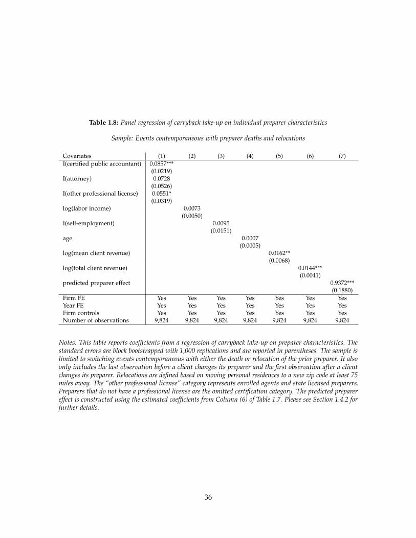
Table 1.8: Panel regression of carryback take-up on individual preparer characteristics

Sample: Events contemporaneous with preparer deaths and relocations

Covariates (1) (2) (3) (4) (5) (6) (7)I(certified public accountant) 0.0857***

(0.0219)I(attorney) 0.0728

(0.0526)I(other professional license) 0.0551*

(0.0319)log(labor income) 0.0073

(0.0050)I(self-employment) 0.0095

(0.0151)age 0.0007

(0.0005)log(mean client revenue) 0.0162**

(0.0068)log(total client revenue) 0.0144***

(0.0041)predicted preparer effect 0.9372***

(0.1880)Firm FE Yes Yes Yes Yes Yes Yes YesYear FE Yes Yes Yes Yes Yes Yes YesFirm controls Yes Yes Yes Yes Yes Yes YesNumber of observations 9,824 9,824 9,824 9,824 9,824 9,824 9,824

Notes: This table reports coefficients from a regression of carryback take-up on preparer characteristics. Thestandard errors are block bootstrapped with 1,000 replications and are reported in parentheses. The sample islimited to switching events contemporaneous with either the death or relocation of the prior preparer. It alsoonly includes the last observation before a client changes its preparer and the first observation after a clientchanges its preparer. Relocations are defined based on moving personal residences to a new zip code at least 75miles away. The “other professional license” category represents enrolled agents and state licensed preparers.Preparers that do not have a professional license are the omitted certification category. The predicted preparereffect is constructed using the estimated coefficients from Column (6) of Table 1.7. Please see Section 1.4.2 forfurther details.

36

take-up of the carryback refund.

We address this additional concern with a two-stage least squares estimate with the

deaths and relocations subsample. Intuitively, we instrument for the change in the preparer

effect with the prior preparer characteristic because we think that the change in client

unobservables is unrelated to the prior preparer. To clarify the interpretation of our

identifying assumption, we express our estimates for this design in a first-differences

version of Equation 1.2.27 We also index our notation by event time e.28

∆I(carryback take-up)ije = ∆ZJ(i,e)γ + ∆Xieβ + ∆δT(i,e) + ∆εie (1.5)

The difference in the equation above is between the first observation after the switching event

and the last observation before the event. These observations are not always consecutive

because firms are not eligible for the carryback refund in every year. We use the following

instrument for the change in the preparer characteristic ∆ZJ(i,e).

∆Z̃J(i,e) = Z̄− ZJ(i,e−1) (1.6)

Our instrument ∆Z̃J(i,e) equals the difference between the sample mean Z̄ and the preparer

characteristic ZJ(i,e−1) from the pre-event period.

The two-stage least squares estimates identify the causal treatment effect of preparer

covariates under the following assumption.

Assumption 2 [Deaths and Relocations Instrument]: The instrument ∆Z̃J(i,e)

must satisfy the exclusion restriction E[∆εie|∆Z̃J(i,e), ∆Xie, ∆δT(i,e)] = 0.

The condition above implies that the change in client unobservables is uncorrelated with the

characteristics of the prior preparer (as represented by the instrument ∆Z̃J(i,e)), the change

in client observables, and the tax year fixed effects. We find it plausible that our setting

satisfies this assumption because we do not believe that changes in client unobservables

27The estimates from a fixed effects specification and a first-differences specification are numerically equiva-lent when the panel has two observations per firm.

28The function T(i, e) maps firm i at event time e to tax year t.

37

determine preparer deaths and relocations.

We report results from the instrument design for the predicted preparer effect.29 We

do not include results for the individual preparer covariates because we lack the statistical

power to estimate informative coefficients for them. Our subsample only includes 9,824

observations, 8 percent of the sample with all switching events. We have more statistical

power with the predicted preparer effect because it combines the individual covariates into

one summary statistic.

Table 1.9 reports our two-stage least squares estimates. Each column represents a

different regression. All regressions include a client fixed effect. Column (2) adds a tax year

fixed effect. Column (3) adds firm controls. We include dummies for missing values of

the client controls. The standard errors are block bootstrapped by firm30 and reported in

parentheses.

We expect to find a coefficient of one on the predicted preparer effect. As stated earlier,

the predicted preparer effects captures the estimated relationship between the preparer

covariates and carryback take-up. Our estimates will not mechanically equal one, however,

because they are based on a different research design.

We find point estimates of 1.1780, 0.9950, and 0.7532 in columns (1), (2), and (3). The

confidence intervals are relatively large, but in all specifications we can reject the null of a

zero coefficient at a 5 percent level. Our estimates are not statistically distinguishable from

a coefficient of one. These results validate the predicted preparer effect estimated under the

switchers design.

1.4.3 Variance of Unobserved Preparer Effect

We have shown that claiming behavior depends on observable preparer characteristics,

but these results most likely understate the impact of preparers on take-up. Preparer

unobservables could have large impacts on client claiming decisions. For example, preparers

29We obtain the estimated coefficients γ̂ from Column (6) of Table 1.7.

30We bootstrap with 1,000 replications.

38

Table 1.9: Two-stage least squares estimates of carryback take-up on predicted preparer effect

Sample: Events contemporaneous with preparer deaths and relocations

Covariates (1) (2) (3)predicted preparer effect 1.1780*** 0.9950*** 0.7532**

(0.3839) (0.3774) (0.3728)Firm FE Yes Yes YesYear FE No Yes YesFirm controls No No YesNumber of observations 9,824 9,824 9,824

Notes: This table reports coefficients from a two-stage least squares regression of carryback take-up onpreparer characteristics. The standard errors are block bootstrapped with 1,000 replications and are reportedin parentheses. The predicted preparer effect is constructed using the estimated coefficients from Column(6) of Table 1.7. The instrument equals the preparer covariate in the pre-event period and the sample meanfor the preparer covariate in the post-event period. All regressions include a firm fixed effect. Column (2)adds a tax year fixed effect. Column (3) adds firm controls, which include log(eligible refund), log(revenue),log(assets), and log(EBITDA). The sample is limited to switching events contemporaneous with either thedeath or relocation of the prior preparer. It also only includes the last observation before a client changes itspreparer and the first observation after a client changes its preparer. Relocations are defined based on movingpersonal residences to a new zip code at least 75 miles away. Please see Section 1.4.2 for further details.

could differ in their familiarity with the tax loss rules or in their beliefs about the audit risk

associated with carryback refunds. For either example, we do not have direct measures of

the unobserved heterogeneity. In this section, we estimate the variance of an unobserved

preparer effect and benchmark our results against the variance of predicted take-up from

client observables.

We use an analysis of variance approach to find the standard deviation of the unobserved

preparer effect. We isolate the preparer variance from the within-firm covariances for pairs

of observations that do and do not share the same preparer. In the former case, we think

that the covariance partly reflects the preparer variance. In the latter, we think that it does

not. The difference between these two covariances estimates the preparer variance.

We use the sample of C corporations eligible for a carryback refund of at least $1,000

between 1998 and 2011. We define take-up as a function of firm characteristics and a

39

preparer fixed effect in Equation 1.7.

I(carryback take-up)ijt = Witπ + µJ(i,t) + ηit (1.7)

In the equation above, firm characteristics Wit include deciles in the eligible carryback

refund, deciles in revenue, deciles in assets, deciles in payroll, state-year fixed effects,

and industry-year fixed effects. We then compute residual take-up with respect to firm

observables.

Tijt = I(carryback take-up)ijt −Witπ = µJ(i,t) + ηit (1.8)

We construct the residuals by estimating Equation 1.7.

We next estimate the within-firm covariance structure of the residual Tijt. We make the

following assumptions of independence and stationarity to arrive at our estimate for the

preparer variance.

Assumption 3 [Independence]: The unobserved preparer effect µJ(i,t) and the

error term ηit are independent.

Assumption 4 [Stationarity]: The covariance between any two error terms,

Cov (εit, εis), equals σ2ε,|t−s|.

We use these assumptions to isolate the preparer variance from the within-firm covariance

structure by differentiating between pairs of observations that do and do not share the same

preparer.

σj=k|t−s| = Cov

(Tijt, Tiks

)= σ2

µ + σ2ε,|t−s|

σj 6=k|t−s| = Cov

(Tijt, Tiks

)= σ2

ε,|t−s|

(1.9)

We find the preparer variance by taking the difference between the two equations above.

We make a strong assumption with the independence condition. It may not hold because

sophisticated clients likely hire sophisticated preparers. But if the firm error term and the

preparer effect are positively correlated as we suspect, our estimate for the preparer variance

provides an upper bound for the true variance. In this sense, our estimate is useful as a

metric for the potential magnitude of the unobserved preparer effect.

40

Figure 1.7 plots our estimates of the within-firm covariances separately for observations

that do and do not share the same preparer. Figure 1.8 plots our estimate for the standard

deviation of the preparer effect. We also report the point estimates and standard errors in

Table 1.10. We block bootstrap the standard errors by firm.31

We find drift in both series of covariance estimates in Figure 1.7. The covariances

decline as the lapsed time between observations increases. This pattern could arise if client

unobservables, such as management practices, slowly change over time. Our estimates

for the preparer variance comes from the difference between the two series in Figure 1.7.

Despite their overall decline, the difference remains relatively stable over time.

The standard deviation of the preparer effect in Figure 1.8 equals the square root of

the difference between the within-firm covariances. The point estimates in the series range

between 0.1303 and 0.1659. Most are statistically indistinguishable. Their weighted average

equals 0.1472.32 This magnitude is larger than any of our estimated effects of the individual

preparer covariates.

We benchmark our result by comparing it to the predicted effect from firm observables

Witπ̂. We find similar variance estimates for the unobserved preparer effect and the

prediction from firm observables. Both estimates equal 9 percent of the variance in take-up

of the carryback refunds.

Alternatively, we can also interpret our result by calculating the implied change in

take-up if a client moved from the 10th percentile to the 90th percentile in preparer effects.

Assuming that the preparer effects follow a normal distribution, take-up would increase

by 38 percentage points. This change would be larger than the baseline take-up rate of 37

percent in the population. These estimates imply that preparers potentially play a substantial

role in determining whether their clients claim the carryback refund.

31We bootstrap with 1,000 replications.

32The weights equal the number of pairs of observations at each time interval, as defined by the length oftime between observations.

41

Figure 1.7: Estimates of within-firm covariances of residual carryback take-up

●

●

2 4 6 8 10 12

0.00

0.02

0.04

0.06

0.08

0.10

years between tax returns

with

in−

firm

cov

aria

nce

●

●

●

●●

●

●

●

●●

●

●●

● same accountantdifferent accountant

Notes: This figure reports the within-firm covariances of residual carryback take-up. Standard errors are blockbootstrapped with 1,000 replications. The estimates are based on the residual Tijt = I(carryback take-up)−Witπ where Wit are client observables. The coefficients π are estimated from a regression of take-up on clientobservables and a preparer fixed effect. Client observables include deciles in the eligible carryback refund, decilesin revenue, deciles in assets, deciles in payroll, state-year fixed effects, and industry-year fixed effects. Weestimate covariances for pairs of observations from the same firm. We differentiate between pairs by the lengthof time between observations and by whether the observations share the same preparer. Please see Section 1.4.3for further details.

42

Figure 1.8: Estimates for standard deviation of preparer effects

●

●

2 4 6 8 10 12

0.00

0.05

0.10

0.15

0.20

0.25

0.30

years between tax returns

estim

ate

for

stan

dard

dev

iatio

n of

pre

pare

r ef

fect

● ●

● ●●

●●

● ●●

●●

●

Notes: This figure plots estimates of the standard deviation of the preparer effect. Standard errors are blockbootstrapped with 1,000 replications. We estimate the variance of the preparer effect by taking the difference ofthe within-firm covariances for pairs of observations that do and do not share the same preparer. (Please seeFigure 1.7.) We then take the square root of the difference to estimate the standard deviation. Please see Section1.4.3 for further details.

43

Table 1.10: Estimates of within-firm covariances

Years Estimate of Estimate ofbetween Same Different preparer preparer

tax returns preparer preparers variance std. dev.1 0.0890 (0.0005) 0.0720 (0.0015) 0.0170 (0.0016) 0.13032 0.0731 (0.0008) 0.0554 (0.0017) 0.0177 (0.0018) 0.13303 0.0697 (0.0009) 0.0459 (0.0017) 0.0238 (0.0019) 0.15434 0.0666 (0.0012) 0.0419 (0.0018) 0.0247 (0.0022) 0.15705 0.0653 (0.0014) 0.0396 (0.0021) 0.0257 (0.0026) 0.16036 0.0632 (0.0016) 0.0346 (0.0020) 0.0287 (0.0025) 0.16937 0.0593 (0.0017) 0.0324 (0.0021) 0.0269 (0.0026) 0.16398 0.0544 (0.0018) 0.0265 (0.0021) 0.0279 (0.0027) 0.16719 0.0506 (0.0021) 0.0227 (0.0023) 0.0278 (0.0032) 0.1669

10 0.0530 (0.0024) 0.0240 (0.0025) 0.0289 (0.0034) 0.170111 0.0498 (0.0030) 0.0238 (0.0031) 0.0259 (0.0043) 0.160912 0.0592 (0.0046) 0.0350 (0.0046) 0.0242 (0.0064) 0.155513 0.0604 (0.0066) 0.0329 (0.0064) 0.0275 (0.0093) 0.1659

weightedaverage 0.0217 0.1472

Notes: This table reports the estimates from an analysis of variance of carryback take-up. Standard errors areblock bootstrapped with 1,000 replications and are reported in parentheses. The estimates are based on theresidual Tijt = I(carryback take-up)−Witπ where Wit are client observables. The coefficients π are estimatedfrom a regression of take-up on client observables and a preparer fixed effect. Client observables include decilesin the eligible carryback refund, deciles in revenue, deciles in assets, deciles in payroll, state-year fixed effects,and industry-year fixed effects. We estimate covariances for pairs of observations from the same firm. Wedifferentiate between pairs by the length of time between observations and by whether the observations sharethe same preparer. We estimate the preparer variance as the difference between covariances for observationsthat do and do not share the same preparer. We estimate the preparer standard deviation as the square root ofthe preparer variance. We compute the weighted average based on the number of pairs per covariance estimate.Please see Section 1.4.3 for further details.

44

1.5 Conclusion

Our study highlights the mediating role that preparers play between the tax code and

taxpayers by showing that preparers influence tax claiming decisions. We use firms that

change preparers to demonstrate that preparer characteristics predict take-up of a corporate

tax refund for losses. We validate our results by focusing on a subsample of events where

the prior preparer either dies or relocates to a new zip code at least 75 miles away. In these

cases, we find it more plausible that client unobservables remain unchanged before and

after the switching event. We also estimate the variance of an unobserved preparer term

and find that it potentially explains as much of the variation in take-up as the prediction

from firm observables.

The results suggest that investing in better take-up of tax benefits could be as important

as changing the tax code itself. Take-up is important for policy design because it directly

impacts the effectiveness of tax benefits. Fiscal stimulus measures in particular often

rely on the introduction of new and temporary tax benefits. For example, the American

Reinvestment and Recovery Act of 2009 distributed 36 percent of its stimulus dollars

through 55 different tax benefits (The Recovery Accountability and Transparency Board

2014). Future research should consider whether targeting preparers with informational

materials or training programs can improve the take-up of tax benefits.

45

Chapter 2

Do Financial Frictions Amplify Fiscal

Policy? Evidence from Business

Investment Stimulus1

2.1 Introduction

Going back to Hall and Jorgenson (1967), economists have asked how taxes affect investment.

The answer is central to the design of countercyclical fiscal policy, since policymakers often

use tax-based investment incentives to spur growth in times of economic weakness. Such

policies often coincide with disruptions in capital markets, so it is natural to ask how taxes

affect investment in the presence of financial frictions. However, the standard theoretical

and empirical treatments assume perfect capital markets.2 This paper uses recent episodes

of investment stimulus to study whether the effect of taxes on investment accords with

1Co-authored with Eric Zwick

2Key theoretical studies include Hall and Jorgenson (1967), Tobin (1969), Hayashi (1982), Abel and Eberly(1994), and Caballero and Engel (1999). Abel (1990) presents a unifying synthesis of the early theoreticalliterature. Key empirical work includes Summers (1981), Auerbach and Hassett (1992), Cummins, Hassett andHubbard (1994), Goolsbee (1998), Chirinko, Fazzari and Meyer (1999), Desai and Goolsbee (2004), Cooper andHaltiwanger (2006), and House and Shapiro (2008). Edgerton (2010) relaxes the frictionless assumption but, incontrast to our study, finds mixed results.

46

the standard, frictionless model. We find that, by ignoring financial frictions, the standard

analysis overlooks a crucial driver of firm responses to tax policy.

The policy we study, “bonus” depreciation, accelerates the schedule for when firms

can deduct from taxable income the cost of investment purchases. Bonus alters the timing

of deductions but not their amount, so the economic incentive created by bonus works

because future deductions are worth less than current deductions. That is, bonus works

because of discounting: firms judge the benefits of bonus by the present discounted value

of deductions over time.3 Speeding up the timing of deductions reduces short term taxes,

but at the expense of higher taxes in the future. With a reasonable risk-adjusted discount

rate, bonus depreciation generates a modest subsidy, so the frictionless model predicts a

small effect of bonus on investment. But in the presence of financial frictions, firms sharply

discount future deductions. Thus financial frictions make bonus more appealing, since the

difference in today’s tax benefits dwarfs the present value comparison that matters in theory.

We study two episodes of bonus depreciation using a difference-in-differences method-

ology to estimate the effect of this policy. We present three empirical findings. First, bonus

depreciation has a substantial effect on investment, much larger than past estimates and

much stronger than the conventional wisdom predicts. Estimates of how tax changes affect

investment vary, but the consensus prediction is that bonus depreciation has a small positive

effect.4 In contrast, we find that bonus depreciation raised eligible investment by 17.3

percent on average between 2001 and 2004 and 29.5 percent between 2008 and 2010. We

estimate a user cost elasticity of approximately -1.6, outside the range of estimates of -0.5

to -1 surveyed by Hassett and Hubbard (2002) and more than double the consensus point

3Summers (1987) states this most clearly: “It is only because of discounting that depreciation schedulesaffect investment decisions. . . ”

4Cummins, Hassett and Hubbard (1994) study many corporate tax reforms and public company investmentdata and conclude that tax policy has a strong effect on investment. Using similar data and a different empiricalmethodology, Chirinko, Fazzari and Meyer (1999) argue that tax policy has a small effect on investment and thatCummins, Hassett and Hubbard (1994) misinterpret their results. Hassett and Hubbard (2002) survey empiricalwork and conclude that the range of estimates for the user cost elasticity has narrowed to between -0.5 and -1.Surveying this and more recent work, Bond and Van Reenen (2007) decide “it is perhaps a little too early toagree with Hassett and Hubbard (2002) that there is a new ‘consensus’ on the size and robustness of this effect.”

47

estimate.5

The first part of the paper details this finding and a litany of robustness tests. The

research design compares firms at the same point in time whose benefits from bonus differ.

Our strategy exploits technological differences between firms in narrowly defined industries.

Firms in industries with most of their investment in short duration categories act as the

“control group” because bonus only modestly alters their depreciation schedule. This natural

experiment separates the effect of bonus from other economic shocks happening at the

same time. If the parallel trends assumption holds—if investment growth for short and

long duration industries would have been similar absent the policy—then the experimental

design is valid.

The key threat to this design is that time-varying industry shocks may coincide with

bonus. This risk is limited for four reasons. First, graphical inspection of parallel trends

indicates smooth pretrends and a clear, steady break for short and long duration firms

during both the 2001 to 2004 and 2008 to 2010 bonus periods. The effects are the same size

in both periods, though different industries suffered in each recession. Second, the estimates

are stable across many specifications and after including firm-level cash flow controls,

industry Q, and flexible industry trends. Controlling for industry-level co-movement with

the macroeconomy actually increases our estimates. Third, the estimates pass a placebo test:

the effect of bonus on ineligible investment is indistinguishable from zero. Last, for firms

making eligible investments, bonus take-up rates (i.e., do firms fill in the bonus box on the

tax form?) are indeed higher in long duration industries. For these reasons, spurious factors

are unlikely to explain the large effect of bonus.

Firms respond to bonus depreciation as if they apply implausibly high discount rates to

investment decisions. This finding is inconsistent with a frictionless model of firm behavior.

In the second part of the paper, we explore alternative models that generate high effective

discount rates by adding financial frictions.6 One alternative is costly external finance,

5In Appendix Section B.3, we collect estimates from past studies of tax reforms. The average user costelasticity across these studies is -0.69.

6We use the term financial frictions as an umbrella term over a class of models that generate high effective

48

which raises the total discount rate firms apply to evaluate projects. Another alternative is

managerial myopia, which raises effective discount rates by sharply discounting the future

relative to the present. Both models prove useful in explaining our findings.

Our second empirical finding is that, consistent with the costly external finance story,

financial constraints amplify the effects of investment stimulus. Nearly all prior empirical

tests of financial constraints use public firm data, which is problematic because public firms

have the best collateral, the strongest banking relationships and broad access to equity and

bond markets.7 In contrast, we work with an analysis sample of more than 120,000 public

and private companies drawn from two million corporate tax returns. Half the firms in our

sample are smaller than the smallest firms in Compustat.8 Our baseline estimate therefore

averages over substantial heterogeneity in firm type, including many firms likely to face

financial constraints.

The largest firms in our sample, those most like the firms in past studies, yield estimates

in line with the Hassett and Hubbard (2002) range. In contrast, small and medium-sized

firms, previously unstudied, show much stronger responses. Building on the differential

response by firm size, we perform a split sample analysis using several markers of ex ante

financial constraints. In addition to small firms, non-dividend payers and firms with low

cash holdings are 1.5 to 2.6 times more responsive than their unconstrained counterparts.

Moreover, we find that firms respond by borrowing and cutting dividends. These facts do

not match the frictionless model of investment behavior, in which firms divided by financial

constraint markers do not respond differently to bonus.

Firms with tax losses must wait to realize the benefits of tax breaks. Because many firms

in our sample are in a tax loss position when a policy shock occurs, we can ask whether firms

discount rates. Some of these—such as managerial myopia and agency theory—are not about external financeper se, but refer instead to organizational frictions.

7Kaplan and Zingales (1997) find that very few of Fazzari, Hubbard and Petersen’s (1988a) most constrainedfirms appear constrained by other measures.

8When aggregated, these small firms account for a large amount of economic activity. According to Censustabulations in 2007 (http://www.census.gov/econ/susb/data/susb2007.html), firms with less than$100 million in receipts (around the 80th percentile in our data) account for more than half of total employmentand one third of total receipts.

49

value future cash windfalls, namely, the larger deductions bonus depreciation provides them

in later years. Our third empirical finding is that, consistent with the managerial myopia

story, firms only respond to investment incentives when the policy immediately generates

cash flows. This finding holds even though firms can carry forward unused deductions

to offset future taxes, and it cannot be explained by differences in growth opportunities.

Furthermore, this fact contradicts a simple model of costly external finance, because firms

neglect how the policy affects borrowing in the future.

To confirm the myopia story, we study a second component of the depreciation schedule.

Firms making small investment outlays face a permanent kink in the tax schedule, which

creates a discontinuous change in marginal investment incentives. This sharp change in

incentives induces substantial investment bunching, with many firms electing amounts

within just a few hundred dollars of the kink. And when legislation raises the kink, the

bunching pattern follows. Consistent with myopia, bunching strongly depends on a firm’s

current tax status: firms just in positive tax position are far more likely to bunch than

firms on the other side of the discontinuity. For a different group of firms and a different

depreciation policy, we again find that firms ignore future tax benefits.

These facts do not match the predictions of a frictionless model, which cannot account

for the large baseline response, the differential response for constrained firms or the

nonresponse for nontaxable firms. The facts point instead toward models in which costly

finance matters and current benefits outweigh future benefits. We use an investment model

to clarify these findings. The model incorporates costly external finance and managerial

myopia into a general model in which the frictionless model of Hayashi (1982) is a special

case. These alternative theories make predictions about the discount rate firms apply to

future cash flows. The model shows how to combine reduced form estimates to distinguish

the frictionless benchmark from costly external finance and managerial myopia.

The general model yields a set of theoretical moments—one comparing constrained

and unconstrained firms and one comparing taxable and nontaxable firms—which we can

combine with our empirical findings to measure financial frictions. With these comparisons

50

we can compute the shadow cost of external funds and an implied present versus future

discount factor. We estimate the shadow cost of external funds to be between $0.63 and

$1.61 per dollar and an implied discount factor of 0.82. Combining these results, financially

constrained firms act as if $1 next year is worth just 38 cents today, yielding a total discount

rate of 97 percent. Thus accounting for the effect of bonus depreciation on investment

requires a major role for financial frictions.

Our paper sits at the intersection of several strands in the economics and finance litera-

tures. Most directly, the paper relates to studies of the effect of taxes on business investment.

Our data improve on past studies by including two periods of bonus depreciation; a granular

breakdown of eligible investment; a large sample of small, private firms; and better tax

variables. Earlier studies pool the effects of different tax reforms, which include depreci-

ation changes, tax rate changes and rule changes regarding corporate form. We focus on

one specific policy, bonus depreciation, and carefully dissect how firms respond.9 In the

literature on salience and taxation, our study offers an example of a strong tax policy effect

on economic behavior.10

Cummins, Hassett and Hubbard (1995) and Edgerton (2010) note that tax losses will

reduce the incentive of firms to respond to tax changes. The former study uses a sample of

sixty loss firms to conclude that losses reduce the effect of tax breaks on investment. The

latter maps financial accounting data to a tax account and finds mixed evidence that losses

matter.11 With our data, we can precisely measure whether a firm’s current tax position

means that the next dollar of investment affects this year’s tax bill. Our sample of loss firms

includes almost two hundred thousand loss year observations.

9House and Shapiro (2008) study the first episode of bonus depreciation using aggregate investment data.

10Our evidence is consistent with the strong behavioral response to and salience of the Earned Income TaxCredit (Chetty, Friedman and Saez, 2013). It stands, for instance, in contrast to evidence that individuals reactincompletely to obscure taxes (Chetty, Looney and Kroft, 2009) and that business investment does not react tochanges in the dividend tax (Yagan, 2013).

11Recent work documents large differences between “book” and tax accounts, which introduces the risk ofmeasurement error into such a mapping (see, e.g., Mills, Newberry and Trautman (2002)). Edgerton (2010) isvery careful with this procedure, but acknowledges that “[one] cannot rule out, however, the possibility thatdifficulties in measuring firms’ taxable status drive the relative unimportance of taxable status observed in theCompustat data.”

51

The paper also relates to the literature on financial constraints.12 We use depreciation

changes as a plausibly exogenous financial constraint shock.13 Unlike past studies, our

instrument also changes the relative price of investment. We use this feature and an

investment model to compute the implied shadow price of internal funds. Our findings

imply that incorporating financial frictions adds much explanatory power to neoclassical

investment theory.

The outline of the paper is as follows. Section 2.2 formalizes intuition about how bonus

works and develops a set of testable hypotheses, which guide the empirical analysis. Section

2.3 describes the corporate tax data, variable construction and sample selection process.

Section 2.4 describes the main empirical strategy for studying bonus depreciation, the

identification assumptions and presents results and robustness tests. Section 2.5 uses split

sample tests by markers of financial constraints and by tax position to show financial frictions

can account for the large baseline effect of bonus. We then develop a set of theoretical

moments and combine the empirical results to compute implied discount rates. Section 2.6

discusses policy implications and avenues for future research.

2.2 Hypothesis Development

To direct our empirical analysis, we develop a simple model of investment in the presence

of depreciation incentives, financial constraints and heterogeneous tax positions. We modify

the neoclassical investment model with adjustment costs (Abel, 1982; Hayashi, 1982) by

introducing an external finance wedge and managerial myopia. Here, we focus on the

intuition of the model and the mapping from theory to empirical objects and tests. We use a

12Fazzari, Hubbard and Petersen (1988a) argue that, if firms more likely to be financially constrained respondmore strongly to cash flow shocks, then financial constraints are responsible. Subsequent studies make thisargument while identifying quasi-experimental variation in cash flows or credit supply (Lamont, 1997; Rauh,2006; Chaney, Sraer and Thesmar, 2012). We apply this insight to the case of bonus depreciation. Stein (2003)surveys models in which financial frictions influence investment decisions.

13See the conclusion of Fazzari, Hubbard and Petersen (1988a) and Fazzari, Hubbard and Petersen (1988b)for a discussion of how taxes might affect investment in the presence of financial constraints. They focus onaverage tax rates more generally and do not perform an empirical analysis along these lines.

52

simple one-shot static investment model with a reduced form credit wedge.14 In Appendix

Section B.1, we derive the hypotheses in an infinite horizon setting with adjustment costs

and a dynamic leverage constraint.

Consider a firm making a one shot investment decision. The firm begins with initial

profits π0 and chooses a level of investment I to determine the capital stock and hence

future profits. Future profits are given by π(I), taxed at the proportional corporate tax rate

τ. The firm discounts future flows at risk-adjusted rate r.

The tax code permits the firm to write off the cost of investment over time. The value of

these deductions depends on the tax rate and how the schedule interacts with the firm’s

discount rate. We collapse the stream of future depreciation deductions owed for investment:

z0(β) = D0 + βT

∑t=1

1(1 + r)t Dt (2.2.1)

where Dt is the allowable deduction per dollar of investment in period t and T is the class

life of investment. z0(β) measures the present discounted value of one dollar of investment

deductions before tax. If the firm can immediately deduct the full dollar, then z0 equals one.

Because of discounting, z0 is lower for longer lived items (i.e., items with greater T), which

forms the core of our identification strategy.

In general, the stream of future deductions depends on future tax rates and discount

rates. Our empirical analysis assumes the effective tax rate does not change over time,

except when the firm is nontaxable.15 For discount rates, we apply a risk-adjusted rate of

seven percent for r to compute z0 in the data, which enables comparison to past work. In

Section 2.5.3 we compute the implied additional discount firms apply to future deductions

because of costly finance. β is an additional discount term between zero and one, which

14This wedge is a reduced form model of a set of capital market frictions, which might reflect, for example,costly monitoring problems or adverse selection (Stein, 2003).

15We use the top statutory tax rate in the set of specifications requiring a tax rate. This is an upper bound onthe more realistic effective marginal tax rate, which in turn depends on tax rate progressivity and the level ofother expenses relative to taxable income. See, e.g., Graham (1996, 2000) for a method tracing out the marginaltax benefit curve. The policies we study will increase the use of investment as a tax shield regardless of wherethe firm is on this marginal benefit curve. Except when current and all future taxes are zero, bonus increasesthe marginal tax benefit of investment.

53

reflects the possibility of myopia.16 We use our heterogeneity analysis to identify this term

separately.

Bonus depreciation allows the firm to deduct a per dollar bonus, θ, at the time of the

investment and then depreciate the remaining 1− θ according to the normal schedule:

z(β) = θ + (1− θ)z0(β) (2.2.2)

At different points in time, Congress has set θ equal to 0, 0.3, 0.5 or 1. We use these policy

shocks to identify the effect of bonus depreciation on investment. Industries differ by

average z0 prior to bonus, providing the basis for identification in a difference-in-differences

setup with continuous treatment.

We further generalize z by incorporating a nontaxable state. When the next dollar

of investment does not affect this year’s tax bill, then the firm must carry forward the

deductions to future years.17 Our general z reflects this case:

z(β, γ) = γz(β) + (1− γ)βφz(1), (2.2.3)

where γ ∈ {0, 1} is an indicator for current tax state and φ is a discounter that reflects both

the expected arrival time of the taxable state and the discount rate applied to the future and

subsequent periods when the firm switches. Note that for the nontaxable firm, β applies

to all future deductions. Even when β equals one, φ is less than one, so the value of these

deductions are lower when the firm is nontaxable. We measure φ in the data and apply our

split sample results to determine whether we can justify our findings in a model without

myopia.

External finance matters for all investment exceeding current cash flow. During the

16The myopia model is closer to Akerlof (1991) and Laibson (1997) than it is to the model of managerialmyopia in Stein (1989). Stein’s (1989) model of managerial myopia specifically refers to the incentive to boostcurrent earnings as a way of signaling high quality to the stock market. We use the term to reflect any motive toboost current earnings and neglect projects with long term payoffs and short term costs.

17This assumes that “carrybacks”—in which firms apply unused deductions this year against past taxbills—have been exhausted or ignored. Relaxing this assumption complicates notation without altering thepuzzle of a low response for nontaxable firms.

54

investment period, the firm faces an external finance wedge that is linear in expenses net of

cash flows, that is,

c(I) = λ [(1− τz)I − (1− τ)π0] , (2.2.4)

where λ can be thought of as the shadow price on a borrowing constraint that may or

may not bind now or in the future. Thus a dollar of cash inside the firm is worth 1 + λ.18

We include z in the net expense term rather than the first year deduction to capture the

influence of depreciation deductions on future taxes and thus future borrowing. While

bonus depreciation relaxes the current constraint through reducing this year’s tax bill,

it does so at the expense of higher future taxes. The net effect is to reduce the present

discounted borrowing costs for the firm. However, if myopia plays a role (that is, for low

β), then only the current year change will matter. The two models thus yield different

predictions for constrained, nontaxable firms: constrained, myopic firms respond much less

to bonus when nontaxable than do constrained, farsighted firms. This is the feature we use

to distinguish costly external finance from myopia models.

Though the problem occurs over time, we can write it as a static one shot investment

problem by discounting future flows to the present. Discarding elements not involving

investment, the firm’s objective is

maxI

{(1− τ)π(I)

1 + r− (1− τz)I − λ(1− τz)I

}(2.2.5)

We assume π is weakly concave, which ensures that the problem yields a unique interior

solution.

The first order condition for optimal investment is

(1− τ)π′(I∗) = (1 + r)(1 + λ)(1− τz). (2.2.6)

Intuitively, the investment decision trades off the after-tax future benefits of the marginal

18Note that because we have assumed a linear external finance function, there will be no direct effect of cashflows on investment, that is, the investment-cash flow sensitivity is zero. Because each dollar of investment canonly generate at most 35 cents of cash back, these policies cannot operate mainly through a direct cash windfallchannel.

55

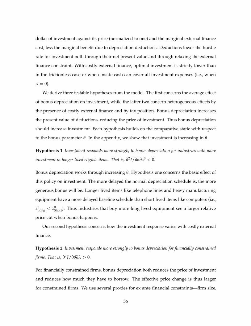
dollar of investment against its price (normalized to one) and the marginal external finance

cost, less the marginal benefit due to depreciation deductions. Deductions lower the hurdle

rate for investment both through their net present value and through relaxing the external

finance constraint. With costly external finance, optimal investment is strictly lower than

in the frictionless case or when inside cash can cover all investment expenses (i.e., when

λ = 0).

We derive three testable hypotheses from the model. The first concerns the average effect

of bonus depreciation on investment, while the latter two concern heterogeneous effects by

the presence of costly external finance and by tax position. Bonus depreciation increases

the present value of deductions, reducing the price of investment. Thus bonus depreciation

should increase investment. Each hypothesis builds on the comparative static with respect

to the bonus parameter θ. In the appendix, we show that investment is increasing in θ.

Hypothesis 1 Investment responds more strongly to bonus depreciation for industries with more

investment in longer lived eligible items. That is, ∂2 I/∂θ∂z0 < 0.

Bonus depreciation works through increasing θ. Hypothesis one concerns the basic effect of

this policy on investment. The more delayed the normal depreciation schedule is, the more

generous bonus will be. Longer lived items like telephone lines and heavy manufacturing

equipment have a more delayed baseline schedule than short lived items like computers (i.e.,

z0Long < z0

Short). Thus industries that buy more long lived equipment see a larger relative

price cut when bonus happens.

Our second hypothesis concerns how the investment response varies with costly external

finance.

Hypothesis 2 Investment responds more strongly to bonus depreciation for financially constrained

firms. That is, ∂2 I/∂θ∂λ > 0.

For financially constrained firms, bonus depreciation both reduces the price of investment

and reduces how much they have to borrow. The effective price change is thus larger

for constrained firms. We use several proxies for ex ante financial constraints—firm size,

56

dividend payment activity and liquid asset positions—to test for a difference in elasticities

between constrained and unconstrained firms. If financial constraints are unimportant, then

we should not find a consistent, systematic difference in elasticities for groups of firms

based on these proxies. We can also use the difference in coefficients between constrained

and unconstrained firms to infer the implied external finance spread. We formalize and

implement this intuition in Section 2.5.3.

Our third hypothesis concerns how the investment response varies with the firm’s

current tax position.

Hypothesis 3 Investment responds more strongly to bonus depreciation for firms with current-year

taxable income. That is, ∂I/∂θ|γ=1 > ∂I/∂θ|γ=0.

Hypothesis three emerges in any model with some positive discounting, since future benefits

are worth less than immediate benefits. The main value of the comparison between taxable

and nontaxable groups derives from the calibration it offers. We can calibrate the expected

arrival of the taxable state for nontaxable firms and ask whether the difference between

elasticities for taxable and nontaxable firms requires some myopia (i.e., β < 1).

2.3 Business Tax Data

The analysis in this paper uses the most complete dataset yet applied to study business

investment incentives.19 The data include detailed information on equipment and structures

investment, offering a finer breakdown than previously available for a broad class of

industries. The sample includes many small, private firms and all of the largest US firms,

which enables the heterogeneity analysis we use to document financial constraints. Because

the data come from corporate tax returns, we can separate firms based on whether the next

dollar of investment affects this year’s taxes. This allows a split sample analysis that can

distinguish the myopia model from a simple model of costly external finance. In this section,

19Yagan (2013) uses these data to study the 2003 dividend tax cut. Kitchen and Knittel (2011) use these datato describe general patterns in bonus and Section 179 take-up.

57

we describe where these data come from and the analysis sample, as well as how we map

the theory into empirical objects.

Sampling Process. Each year, the Statistics of Income (SOI) division of the IRS Research,

Analysis and Statistics unit produces a stratified sample of approximately 100,000 unaudited

corporate tax returns.20 Stratification occurs by form type,21 total assets, and proceeds. SOI

uses these samples to generate annual publications documenting income characteristics.

The BEA uses them to finalize national income statistics. In addition, the Treasury’s Office

of Tax Analysis (OTA) uses the sample to perform policy analysis and revenue estimation.

In 2008, the sample represented about 1.8 percent of the total population of 6.4 million C

and S corporation returns. Any corporation selected into the sample in a given year will

be selected again the next year, providing it continues to fall in a stratum with the same

or higher sampling rate. Shrinking firms are resampled at a lower rate, which introduces

sampling attrition. We address this attrition in several ways, including a nonparametric

reweighting procedure for figures and through assessing the robustness of our results in a

balanced panel. Each sample year includes returns with accounting periods ending between

July of that year and the following June. When necessary, we recode the tax year to align

with the implementation of the policies studied in this paper.

Analysis Samples, Variable Definitions and Summary Statistics. We create a panel by

linking the cross sectional SOI study files using firm identifiers.22 The raw dataset has 1.84

million rows covering the years from 1993 to 2010. There are 355 thousand distinct firms in

this dataset, 19,711 firms with returns in each year of the sample and 62,478 firms with at

least 10 years of returns. Beginning with the sample of firms with valid data for each of the

20Details come from http://www.irs.gov/pub/irs-soi/08cosec3ccr.pdf.

21For example, C corporations file form 1120 and S corporations file form 1120S. Other form types includereal estate investment trusts, regulated investment companies, foreign corporations, life insurance companies,and property and casualty insurance companies. We focus on 1120 and 1120S, which cover the bulk of businessactivity in industries making equipment investments.

22We thank Jason Debacker and Rich Prisinzano for providing the data crosswalk.

58

main data items analyzed, we keep firm-years satisfying the following criteria: (a) having

non-zero total deductions or non-zero total income23 and (b) having an attached investment

form.24 In addition, we exclude partial year returns, which occur when a firm closes or

changes its fiscal year. To analyze bonus depreciation, we exclude firms potentially affected

by Section 179, a small firm investment incentive which we analyze separately. Our main

bonus analysis sample consists of all firms with average eligible investment greater than

$100,000 during years of positive investment.25 This sample consists of 820,769 observations

for 128,151 distinct firms.

We describe the economic concepts underlying the variables we study. Eligible invest-

ment, our main variable of interest, includes expenditures for all equipment investment

put in place during the current year for which bonus and Section 179 incentives apply.26

We conduct separate analyses for intensive and extensive margin responses. The intensive

margin variable is the logarithm of eligible investment. The extensive margin variable is an

indicator for positive eligible investment. We aggregate this indicator at the industry level

and transform it into a log odds ratio27 for our empirical analyses. In some specifications,

we use an alternative measure of investment, which is eligible investment divided by lagged

capital stock. Capital stock is the reported book value of all tangible, depreciable assets.

Sales equals operating revenue and assets equals total book assets. Total debt equals the

sum of non-equity liabilities excluding trade credit. Liquid assets equals cash and other

liquid securities. Payroll equals non-officer wage compensation. Rents equals lease and

23Knittel et al. (2011) use a similar “de minimus” test to select business entities that engage in “substantial”business activity.

24Form 4562 is the tax form that corporations attach to their return to claim depreciation deductions on newand past investments. An entity that claims no depreciation deductions need not attach form 4562. It is likelythat these firms do not engage in investment activity, and so their exclusion should not affect the interpretationof results.

25The relevant threshold for Section 179 was $25,000 until 2003, when it increased to $100,000. In 2008, itincreased to $250,000 and then to $500,000 in 2010. Using alternative thresholds in the range from $50,000 to$500,000 does not alter the results.

26Section 179 and bonus rules differ slightly, in that Section 179 also applies to used equipment purchases,while bonus only applies to new equipment. The form does not require firms to list used purchases separately.

27We use log( p1−p ) as our measure of the extensive margin.

59

rental expenses. Interest equals interest payments.

Our main policy variable of interest, zN,t, is the present discounted value of one dollar

of deductions for eligible investment. In each non-bonus year, we compute the share of

eligible investment a firm reports in each category.28 We use these shares and the present

value of one dollar of eligible investment for each category to construct a weighted average,

firm-level z. Category z’s come from applying a seven percent discount rate to the pertinent

deduction schedule,29 while assuming a six-month convention for the purchase year.30 We

compute zN at the four-digit NAICS industry level as the simple average of firm-level z’s

across non-bonus years prior to 2001.31 In bonus years, we adjust z by the size of the bonus.

If θ is the additional expense allowed per dollar of investment (e.g., θ = .3 for 2001), then

zN,t|θt = θt + (1− θt)× zN . The interaction between the time series variation in θ and the

cross sectional variation in zN delivers the identifying variation we use to test our three

hypotheses.

Table 2.1 collects summary statistics for the sample in our bonus depreciation analysis.

The average observation has $6.8 million in eligible investment, $180 million in sales and

$27 million in payroll. The size distribution of corporations is skewed, with median eligible

investment of just $370 thousand and median sales of $26 million. The average net present

value of depreciation allowances, zN,t, is 0.88 in non-bonus years, implying that eligible

investment deductions for a dollar of investment are worth eighty-eight cents to the average

firm. zN,t increases to an average of 0.94 during bonus years. Cross sectional differences in

28Specifically, 3-, 5-, 7-, 10-, 15-, and 20-year Modified Accelerated Cost Recovery System (MACRS) propertyand listed property.

29The category deduction schedules are available in IRS publication 946. We use a seven percent rate as africtionless benchmark that is likely larger than the rate firms should be using, which will tend to bias ourresults downward. Summers (1987) argues that firms should apply a discount rate close to the risk-free ratefor depreciation deductions. Seven percent is the largest discount rate House and Shapiro (2008) apply whencomputing the value of bonus depreciation.

30The six-month convention is applied because on average the property is in place for only half of the firstyear.

31Like Cummins, Hassett and Hubbard (1994) and Edgerton (2010), we proxy for the firm-level benefit ofbonus depreciation with an industry measure of policy benefits. Unlike these studies, our measure derivesdirectly from tax data, reducing measurement error. It is possible to apply the same strategy at the firm level.This approach does not alter our findings.

60

zN,t are similar in magnitude to the change induced by bonus, with zN,t varying from 0.87

at the tenth percentile to 0.94 at the ninetieth. The first year deduction, θN,t, increases from

an average of 0.18 in non-bonus years to 0.58 in bonus years.

The difference in z’s over time of just six cents per dollar before tax translates into

a benefit of just over two cents after tax, which is why some authors claim the effect of

bonus on investment should be small. However, if the discount rate firms apply to future

deductions includes a large external finance wedge or myopia, then this two cent difference

can increase to as much as the fourteen cent difference in average after-tax θs.

It is helpful to give a sense of the groups being compared, because our identification will

be based on assuming that industry-by-year shocks are not confounding the trends between

industry groups. The five most common three-digit industries (NAICS code) in the bottom

three zN deciles are: motor vehicle and parts dealers (441), food manufacturing (311), real

estate (531), telecommunications (517), and fabricated metal product manufacturing (332). In

the top three deciles are: professional, scientific and technical services (541), specialty trade

contractors (238), computer and electronic product manufacturing (334), durable goods

wholesalers (423), and construction of buildings (236). Neither group of industries appears

to be skewed toward a spurious relative boom in the low z group. The telecommunications

industry suffered unusually during the early bonus period as did real estate in the later

period. Both industries are in the group for which we observe a larger investment response

due to bonus.

2.4 The Effect of Bonus Depreciation on Investment

We begin with a test of Hypothesis 1, which predicts that investment responds more strongly

to bonus depreciation for industries with more investment in longer lived eligible items.

In both bonus periods we study, we estimate large responses to bonus depreciation. The

estimates are similar in both periods. We assess the key risk of this design—that time-

varying industry shocks confound our estimates—using a variety of specifications, a placebo

test and differences in policy salience across space.

61

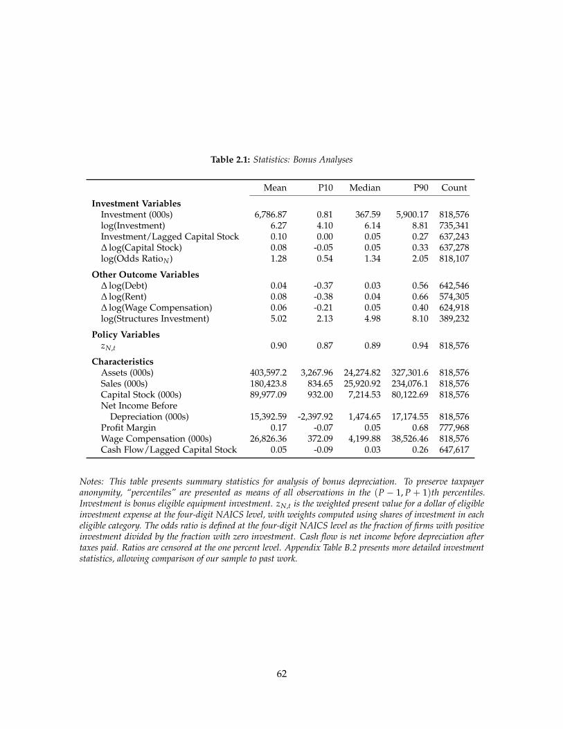
Table 2.1: Statistics: Bonus Analyses

Mean P10 Median P90 Count

Investment VariablesInvestment (000s) 6,786.87 0.81 367.59 5,900.17 818,576log(Investment) 6.27 4.10 6.14 8.81 735,341Investment/Lagged Capital Stock 0.10 0.00 0.05 0.27 637,243∆ log(Capital Stock) 0.08 -0.05 0.05 0.33 637,278log(Odds RatioN) 1.28 0.54 1.34 2.05 818,107

Other Outcome Variables∆ log(Debt) 0.04 -0.37 0.03 0.56 642,546∆ log(Rent) 0.08 -0.38 0.04 0.66 574,305∆ log(Wage Compensation) 0.06 -0.21 0.05 0.40 624,918log(Structures Investment) 5.02 2.13 4.98 8.10 389,232

Policy VariableszN,t 0.90 0.87 0.89 0.94 818,576

CharacteristicsAssets (000s) 403,597.2 3,267.96 24,274.82 327,301.6 818,576Sales (000s) 180,423.8 834.65 25,920.92 234,076.1 818,576Capital Stock (000s) 89,977.09 932.00 7,214.53 80,122.69 818,576Net Income Before

Depreciation (000s) 15,392.59 -2,397.92 1,474.65 17,174.55 818,576Profit Margin 0.17 -0.07 0.05 0.68 777,968Wage Compensation (000s) 26,826.36 372.09 4,199.88 38,526.46 818,576Cash Flow/Lagged Capital Stock 0.05 -0.09 0.03 0.26 647,617

Notes: This table presents summary statistics for analysis of bonus depreciation. To preserve taxpayeranonymity, “percentiles” are presented as means of all observations in the (P − 1, P + 1)th percentiles.Investment is bonus eligible equipment investment. zN,t is the weighted present value for a dollar of eligibleinvestment expense at the four-digit NAICS level, with weights computed using shares of investment in eacheligible category. The odds ratio is defined at the four-digit NAICS level as the fraction of firms with positiveinvestment divided by the fraction with zero investment. Cash flow is net income before depreciation aftertaxes paid. Ratios are censored at the one percent level. Appendix Table B.2 presents more detailed investmentstatistics, allowing comparison of our sample to past work.

62

Policy Background. House and Shapiro (2008) provide a detailed discussion of the baseline

depreciation schedule and legislative history of the first round of bonus depreciation.

Kitchen and Knittel (2011) provide a brief legislative history of the second round.32 Appendix

Section B.2 summarizes the relevant legislation for our sample frame.

In 2001, firms buying qualified investments were allowed to immediately write off 30

percent of the cost of these investments. The bonus increased to 50 percent in 2003 and

expired at the end of 2004. In 2008, 50 percent bonus depreciation was reinstated. It was

later extended to 100 percent bonus for tax years ending between September 2010 and

December 2011. The policies applied to equipment and excluded most structures.33

Consider a firm buying $1 million worth of computers. The firm owes corporate taxes

on income net of business expenses. For expenses on nondurable items such as wages and

advertising, the firm can immediately deduct the full cost of these items on its tax return.

Thus an extra dollar of spending on wages reduces the firm’s taxable income by a dollar

and reduces the firm’s tax bill by the tax rate. But for investment expenses the rules differ.

Usually, the firm follows the regular depreciation schedule in the top panel of Table

2.2. The first year deduction is $200 thousand, which provides an after-tax benefit of $70

thousand. Over the next five years, the firm deducts the remaining $800 thousand. The total

undiscounted deduction is the $1 million spent and the total undiscounted tax benefit is

$350 thousand. With bonus depreciation the situation changes. Assume 50 percent bonus.

The firm can now deduct a $500 thousand bonus before following the normal schedule

for the remaining amount, so the total first year deduction rises to $600 thousand. Each

subsequent deduction falls by half.

The total amount deducted over time does not change. However, the accelerated schedule

does raise the present value of these deductions. Applying a seven percent discount rate

yields $311 thousand for the present value of cash back in normal times. Bonus raises this

32See also the Treasury’s “Report to The Congress on Depreciation Recovery Periods and Methods” (2000).

33These provisions coincided with an increase in the Section 179 allowance for small investments from$24,000 to $100,000 in 2003, from $125,000 to $250,000 in 2008, and from $250,000 to $500,000 in 2010.

63

Table 2.2: Regular and Bonus Depreciation Schedules for Five Year Items

Normal Depreciation

Year 0 1 2 3 4 5 Total

Deductions (000s) 200 320 192 115 115 58 1000Tax Benefit (τ = 35%) 70 112 67.2 40.3 40.3 20.2 350

Bonus Depreciation (50%)

Year 0 1 2 3 4 5 Total

Deductions (000s) 600 160 96 57.5 57.5 29 1000Tax Benefit (τ = 35%) 210 56 33.6 20.2 20.2 10 350

Notes: This table displays year-by-year deductions and tax benefits for a $1 million investment in computers, afive year item, depreciable according to the Modified Accelerated Cost Recovery System (MACRS). The topschedule applies during normal times. It reflects a half-year convention for the purchase year and a 200 percentdeclining balance method (2X straight line until straight line is greater). The bottom schedule applies when50 percent bonus depreciation is available. See IRS publication 946 for the recovery periods and schedulesapplying to other class lives.

present value by $20 thousand, just two percent of the original purchase price. This small

present value payoff is why some authors conclude that bonus provides little stimulus for

short-lived items (Desai and Goolsbee, 2004).34

In a frictionless model, a firm will judge the benefits of bonus by comparing these

present value payoffs. Note however the large difference in the initial deduction, which

translates into $140 thousand of savings in the investment year. Such a difference will matter

if firms must borrow to meet current expenses and external finance is costly. Or it will

matter if managers are myopic in the sense that they will aggressively use bonus to reduce

current taxes even at the expense of higher future taxes. In short, when firms use higher

effective discount rates to evaluate bonus, they will respond more than the frictionless

model predicts.

The policies were intended as economic stimulus. In the words of Congress, “increasing

34See also Steuerle (2008), Knittel (2007) and House and Shapiro (2008). In his comment on Desai andGoolsbee (2004), Kevin Hassett argues that the temporary nature of these policies increases the stimulus throughintertemporal shifting, and that the authors’ results are consistent with a large response; see also Cohen, Hansenand Hassett (2002). The intertemporal shifting story cannot explain our heterogeneity results and predictspatterns which we do not observe.

64

and extending the additional first-year depreciation will accelerate purchases of equipment,

promote capital investment, modernization, and growth, and will help to spur an economic

recovery” (Committee on Ways & Means, 2003, p. 23). To avoid encouraging firms to delay

investment until the policy came online, legislators announced that the policy would apply

retroactively to include the time when the policy was under debate. Although the first

bonus legislation passed in early 2002, firms anticipating policy passage would have begun

responding in the fourth quarter of 2001. We therefore include firm-years with the tax year

ending within the legislated window in our treatment window.

Whether firms perceived the policy as temporary or permanent is a subject of debate.

The initial bill branded the policy as temporary stimulus, slating it to expire at the end of

2004, which it did. For this reason, House and Shapiro (2008) assume firms treat the policy as

temporary. In contrast, Desai and Goolsbee (2004) cite survey evidence indicating that many

firms expected the provisions to continue, and our empirical analysis in Section 2.4 offers

little evidence of intertemporal shifting. Expecting the policy to be temporary is important

for House and Shapiro (2008), because their exercise relies upon how policies approximated

as instantaneous interact with the duration of investment goods approximated as infinitely

lived. Our design relies less on this assumption. In our model, costly external finance

and myopia amplify the effects of both temporary and permanent policies. And our cross

sectional identification also relies less on the response of the longest lived investment goods.

Empirical Setup. Bonus depreciation provides a temporary reduction in the price and

a temporary increase in the first year deduction for eligible investment goods. Eligible

items are classified for deduction profiles over time based on their useful life. Identification

builds upon the idea that some industries benefited more from these cuts by virtue of

having longer duration investment patterns, that is, by having more investment in longer

class life categories. This cross-sectional variation permits a within-year comparison of

investment growth for firms in different industries.35 The policy variation is at the industry-

35This methodological approach was first applied in Cummins, Hassett and Hubbard (1994). See alsoCummins, Hassett and Hubbard (1996), Desai and Goolsbee (2004), House and Shapiro (2008) and Edgerton

65

by-year level, so the key identifying assumption is that the policies are independent of other

industry-by-year shocks. Several robustness tests validate this assumption.

The regression framework implements the difference-in-differences (DD) specification,

f (Iit, Ki,t−1) = αi + βg(zN,t) + γXit + δt + ε it (2.4.1)

where zN,t is measured at the four-digit NAICS industry level and increases temporarily

during bonus years. The specific additive form we adopt in (2.4.1) for the unobserved

firm-level components, αi, can only be valid for a particular class of investment functions.

For example, if valid in levels, the design cannot be valid in logs. The investment data

summarized in Table 2.1 is highly skewed with a mean of $6.8 million and a median of

just $368 thousand. Thus a multiplicative unobserved effect (that is, Ii = Ai I∗(z)) is the

most likely empirical model for investment levels. This delivers an additive model in

logarithms, which is the approach we pursue below. Because approximately eight percent

of our observations for eligible investment are equal to zero, we supplement the intensive

margin logs approach with a log odds model for the extensive margin. We measure the log

odds ratio as log(P[I > 0]/(1− P[I > 0])) at the four-digit industry level.36

Studies often use an alternative empirical specification for f (I, K), where investment

is scaled by lagged assets or lagged capital stock. We prefer log investment for four

reasons. First, small firms are not always required to disclose balance sheet information,

so requiring reported assets would reduce our sample frame. Second, and related to the

first reason, requiring two consecutive years of data for a firm-year reduces our sample

by fifteen percent. Third, there is some concern that balance sheet data on tax accounts

are not reported correctly for consolidated companies due to failure to net out subsidiary

elements.37 Measurement error in the scaling variable introduces non-additive measurement

(2010).

36An alternative specification, with the odds ratio replaced by P[I > 0], works as well. However, the logsodds ratio has better statistical properties (e.g., a more symmetric distribution).

37Mills, Newberry and Trautman (2002) analyze balance sheet accounting in tax data and documentdifficulties in reconciling these accounts with book accounts.

66

error into the dependent variable. Last, with multiple types of capital, the scaling variable

might not remove the unobserved firm effect from the model. This is especially a concern

because we cannot measure a firm’s stock of eligible capital and because firms vary in the

share of total investments made in eligible categories.38 While we prefer the log investment

model, we also report results using investment scaled by lagged capital stock, which allows

comparison to past studies.

Graphical Evidence. Figure 2.1 presents a visual implementation of this research design.

To allow a comparison that matches a regression analysis with fixed effects and firm-

level covariates, we construct residuals from a two-step regression procedure. First, we

nonparametrically reweight (i.e., Dinardo, Fortin and Lemieux (1996) reweight) the group-

by-year distribution within ten size bins based on assets crossed with ten size bins based on

sales.39 This procedure addresses sampling frame changes over time, which cause instability

in the aggregate distribution.40 In the second step, we run cross sectional regressions each

year of the outcome variable on an indicator for treatment group—either long duration or

short duration—and a rich set of controls, including ten-piece splines in assets, sales, profit

margin and age. We plot the residual group means from these regressions.41

We compare mean investment in calendar time for the top and bottom three deciles of

the investment duration distribution.42 Long duration industries show growth well above

that of the short duration industries, with this difference only appearing in the bonus years.

The difference between the slopes of these two lines in any year gives the difference-in-

differences estimate between these groups in that year. The other years provide placebo

38Abel (1990) notes that this issue and other violations of linear homogeneity can lead to spurious conclusions(e.g., a reversed investment-Q relationship).

39The bins are set based on the size distribution in 2000.

40During the period we study, the size of the sample frame changed twice due to budgetary constraints.

41To align the first year of each series and ease comparison of trends, we subtract from each dot the groupmean in the first year and add back the pooled mean from the first year. All means are count weighted.

42Deciles are computed at the industry level.

67

Figure 2.1: Calendar Difference-in-Differences

Intensive Margin: Bonus I Intensive Margin: Bonus II

Extensive Margin: Bonus I Extensive Margin: Bonus II

Notes: The top graphs plot the average logarithm of eligible investment over time for groups sorted according totheir industry-based treatment intensity. Treatment intensity depends on the average duration of investment,with long duration industries (treatment groups) seeing a larger average price cut due to bonus than shortduration industries (control groups). The bottom graphs plot the industry-level log odds ratio for the probabilityof positive eligible investment, thus offering a measure of the extensive margin response. The treatment yearsfor Bonus I are 2001 through 2004 and 2008 through 2010 for Bonus II. In these years, the difference betweenchanges in the red and the blue lines provides a difference-in-differences estimator for the effect of bonus inthat year for those groups. The earlier years provide placebo tests and a demonstration of parallel trends. Theaverages plotted here result from a two-step regression procedure. First, we nonparametrically reweight thegroup-by-year distribution (i.e., Dinardo, Fortin, and Lemieux (1996) reweight) within ten size bins based onassets crossed with ten size bins based on sales to address sampling frame changes over time. Second, we runcross sectional regressions each year of the outcome variable on an indicator for treatment group and a richset of controls, including ten-piece splines in assets, sales, profit margin and age. We plot the residual groupmeans from these regressions. To align the first year of each series and ease comparison of trends, we subtractfrom each dot the group mean in the first year and add back the pooled mean from the first year. All means arecount weighted.

68

tests of the natural experiment and indicate no false positives.

Statistical Results and Economic Magnitudes. Table 2.3 presents regressions of the form

in (2.4.1), where f (Iit, Ki,t−1) equals log(Iit) in the intensive margin model, log(PN [Iit >

0]/(1− PN [Iit > 0])) in the extensive margin model, and Iit/Ki,t−1 in the user cost model;

and g(zN,t) equals zN,t in the intensive and extensive margin models and (1− τzN,t)/(1− τ)

in the user cost model.43 The baseline specification includes year and firm fixed effects.

Standard errors are clustered at the firm level in the intensive margin and user cost models.44

Because log odds ratios are computed at the industry level, standard errors in the extensive

margin model are clustered at the industry level.

The first column reports an intensive margin semi-elasticity of investment with respect

to z of 3.7, an extensive margin semi-elasticity of 3.8 and a user cost elasticity of −1.6. The

average change in zN,t was 4.7 cents during the early bonus period and 8 cents during

the later period, implying average investment increases of 17.3(= 3.69× 4.7) and 29.5(=

3.69 × 8) log points, respectively. These predictions should not be confused with the

aggregate effect of the policy, because they are based on equal-weighted regressions which

include many small firms. They only provide an informative aggregate prediction under

the strong assumption that the semi-elasticity is independent of firm size.

In the second column, including a control for contemporaneous cash flow scaled by

lagged capital does not alter the estimates. Columns three and four show a similar semi-

elasticity for both the early and late episodes. Column five controls for fourth order

polynomials in each of assets, sales, profit margin and firm age, as well as industry average

Q measured from Compustat at the four-digit level. Column six adds quadratic time

trends interacted with two-digit NAICS industry dummies, which causes the estimated

43τ is set to 35 percent, the top statutory tax rate for all firms.

44This is consistent with recent work (e.g., Desai and Goolsbee (2004), Edgerton (2010), Yagan (2013)) andenables us to compare our confidence bands to past estimates. The implicit assumption that errors withinindustries are independent is strong, for the same reason that Bertrand, Duflo and Mullainathan (2004) criticizepapers that cluster at the individual level when studying state policy changes. Our results in this section arerobust to industry clustering, as are the tax splits in the next section. We are not aware of other studies thatrestrict inference in this way and still show that taxes affect investment.

69

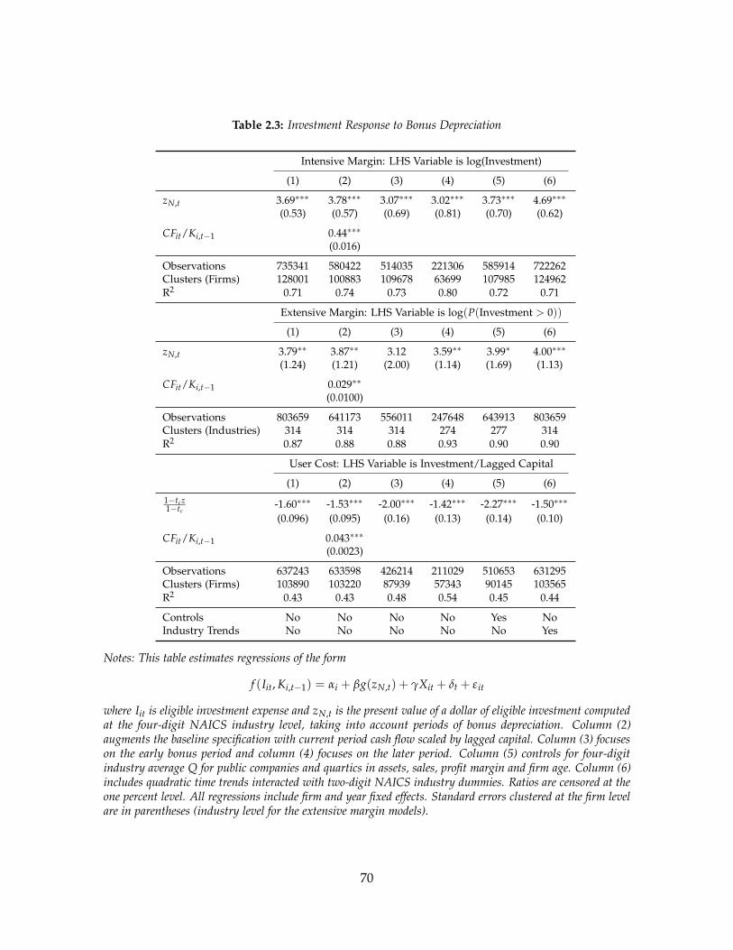
Table 2.3: Investment Response to Bonus Depreciation

Intensive Margin: LHS Variable is log(Investment)

(1) (2) (3) (4) (5) (6)

zN,t 3.69∗∗∗ 3.78∗∗∗ 3.07∗∗∗ 3.02∗∗∗ 3.73∗∗∗ 4.69∗∗∗

(0.53) (0.57) (0.69) (0.81) (0.70) (0.62)

CFit/Ki,t−1 0.44∗∗∗

(0.016)

Observations 735341 580422 514035 221306 585914 722262Clusters (Firms) 128001 100883 109678 63699 107985 124962R2 0.71 0.74 0.73 0.80 0.72 0.71

Extensive Margin: LHS Variable is log(P(Investment > 0))

(1) (2) (3) (4) (5) (6)

zN,t 3.79∗∗ 3.87∗∗ 3.12 3.59∗∗ 3.99∗ 4.00∗∗∗

(1.24) (1.21) (2.00) (1.14) (1.69) (1.13)

CFit/Ki,t−1 0.029∗∗

(0.0100)

Observations 803659 641173 556011 247648 643913 803659Clusters (Industries) 314 314 314 274 277 314R2 0.87 0.88 0.88 0.93 0.90 0.90

User Cost: LHS Variable is Investment/Lagged Capital

(1) (2) (3) (4) (5) (6)1−tcz1−tc

-1.60∗∗∗ -1.53∗∗∗ -2.00∗∗∗ -1.42∗∗∗ -2.27∗∗∗ -1.50∗∗∗

(0.096) (0.095) (0.16) (0.13) (0.14) (0.10)

CFit/Ki,t−1 0.043∗∗∗

(0.0023)

Observations 637243 633598 426214 211029 510653 631295Clusters (Firms) 103890 103220 87939 57343 90145 103565R2 0.43 0.43 0.48 0.54 0.45 0.44

Controls No No No No Yes NoIndustry Trends No No No No No Yes

Notes: This table estimates regressions of the form

f (Iit, Ki,t−1) = αi + βg(zN,t) + γXit + δt + εit

where Iit is eligible investment expense and zN,t is the present value of a dollar of eligible investment computedat the four-digit NAICS industry level, taking into account periods of bonus depreciation. Column (2)augments the baseline specification with current period cash flow scaled by lagged capital. Column (3) focuseson the early bonus period and column (4) focuses on the later period. Column (5) controls for four-digitindustry average Q for public companies and quartics in assets, sales, profit margin and firm age. Column (6)includes quadratic time trends interacted with two-digit NAICS industry dummies. Ratios are censored at theone percent level. All regressions include firm and year fixed effects. Standard errors clustered at the firm levelare in parentheses (industry level for the extensive margin models).

70

semi-elasticity to increase.45 These alternative control sets do not challenge our main finding:

the investment response to bonus depreciation is robust across many specifications.46

Appendix Section B.3 collects from other studies estimates that we can compare to

our user cost model. Like our study, each one uses tax reforms crossed with industry

characteristics to estimate the effect of taxes on investment. Panel (a) of Table 2.2 plots the

estimates from these studies with confidence bands, highlights the consensus range, and

compares them to our estimate. The average user cost elasticity across these studies is -0.69,

which falls within Hassett and Hubbard (2002)’s consensus range of -0.5 to -1, but is less

than half our estimate of 1.60. In an investment model, the elasticity of investment with

respect to the net of tax rate, 1− τz, equals the price elasticity and interest rate elasticity,

derived in Appendix Section B.1. Our empirical model delivers a large elasticity of 7.2. Thus

by several accounts, bonus depreciation has a substantial effect on investment, much larger

than past estimates and much stronger than the conventional wisdom predicts.

Additional Robustness. The calendar time plot in Figure 2.1 provides several visual

placebo tests through inspection of the parallel trends assumption in non-bonus years.

Because bonus depreciation excludes very long lived items (i.e., structures), we can use

ineligible investment as an alternative intratemporal placebo test. The first two columns of

Table 2.4 present two specifications of the intensive margin model, which replace eligible

investment with structures investment. The first specification is the baseline model, and

the second includes two-digit industry dummies interacted with quadratic time trends. We

cannot distinguish the structures investment response from zero. Thus the results pass this

45We can replace the quadratic time trends with increasingly nonlinear trends or two digit industry-by-timefixed effects. We can also replace the time trends with two-digit industry interacted with log GDP or GDPgrowth. In each case, the estimates increase. This suggests that omitted industry-level factors bias our estimatesdownward. Consistent with this story, Dew-Becker (2012) shows that long duration investment falls moreduring recessions than short duration investment.

46We have confirmed these results in a balanced panel and for the sample of firms with enough observationsto compute firm-level zs, which allows inclusion of four-digit industry-by-time fixed effects. Results for theseadditional specifications are available upon request.

71

Figure 2.2: Heterogeneous Effects by Firm Size

(a) Past Estimates

−β

Time

1.0

0.5

0

CHH (1994)

CHH (1996)

DG (2004)

Edge (2010)

Hassett and Hubbard (2002) range

Us

(b) Estimates by Firm Size, Bonus Sample

Hassett and Hubbard (2002) range

Compustat

Notes: These figures plot coefficients and confidence bands from user cost specifications (see the third row ofTable 2.3) for past studies of tax reforms and our sample. The sources for the coefficients in Panel (a) are inAppendix Section B.3. Panel (b) splits the sample into deciles based on mean pre-policy sales. The average firmin Compustat during this time period falls in the tenth size bin (with sales equal to $1.8B), which coincideswith the Hassett and Hubbard (2002) survey range of user cost elasticity estimates (-0.5 to -1).

72

Table 2.4: Investment Response to Bonus Depreciation: Robustness

Structures Net Investment Has Bonus Salience Split

Basic Trends Basic Trends Basic Trends High Low

(1) (2) (3) (4) (5) (6) (7) (8)

zN,t 0.52 1.10 1.07∗∗∗ 0.78∗∗∗ 0.95∗∗∗ 1.15∗∗∗ 5.09∗∗∗ 1.56(0.78) (0.98) (0.23) (0.22) (0.13) (0.16) (0.87) (0.94)

Observations 389232 381921 637278 631680 818576 804128 211390 215205Clusters (Firms) 92351 90166 103447 103147 128150 125534 29627 30836R2 0.59 0.60 0.27 0.27 0.61 0.61 0.70 0.70Industry Trends No Yes No Yes No Yes No No

Notes: This table estimates regressions of the form

Yit = αi + βzN,t + δt + εit

where Yit is either the logarithm of structures investment (columns (1) and (2)), log growth in capital stock(columns (3) and (4)), an indicator for take-up of bonus depreciation ((5) and (6)), or the logarithm of eligibleinvestment ((7) and (8)). zN,t is the present value of a dollar of eligible investment computed at the four-digitNAICS industry level, taking into account periods of bonus depreciation. Columns (1), (3), (5), (7) and (8)implement the baseline specification in table 2.3. Columns (2), (4) and (6) include quadratic time trendsinteracted with two-digit NAICS industry dummies. Columns (7) and (8) split the sample into the top andbottom three deciles according to local geographic salience of the depreciation schedule. We proxy for localsalience using frequency of bunching by small firms at the Section 179 kink point in the depreciation schedule.All regressions include firm and year fixed effects. Standard errors clustered at the firm level are in parentheses.

placebo test.47

Another concern with our results is that they may merely reflect a reporting response,

with less real investment taking place. The third and fourth columns of Table 2.4 provide

a reality check. We replace our measure of investment derived from form 4562 with net

investment, which is the difference in logarithms of the capital stock between year t and

year t− 1. Both the baseline and industry trend regressions confirm our gross investment

results with net investment responding strongly as well.

Columns five and six of Table 2.4 offer a sanity check of our findings. Here, the

dependent variable is an indicator for whether the firm reports depreciation expense in

the specific form item applicable to bonus. Effectively, this is a test for bonus depreciation

47This placebo test is valid if structures are neither complements nor substitutes for equipment. Without thisassumption, the structures test remains useful because observing a structures response equal in magnitude orlarger than the equipment response would indicate that time-varying industry shocks drive our results.

73

take-up. The table indicates that the probability of taking up bonus is strongly increasing in

the strength of the incentive.

Policy Salience. We now present direct evidence that firms take the tax code into account

when making investment decisions. With respect to equipment investment, they pay special

attention to the depreciation schedule and the nonlinear incentives it creates. These nonlinear

budget sets should induce bunching of firms at rate kinks. Consistent with this logic, we

find sharp bunching at depreciation kink points. This evidence supports our claim that

temporary bonus depreciation incentives were also salient.

We study a component of the depreciation schedule, Section 179, which applies mainly

to smaller firms. Under Section 179, taxpayers may elect to expense qualifying investment

up to a specified limit. With the exception of used equipment,48 all investment eligible

for Section 179 expensing is eligible for bonus depreciation. Focusing on Section 179 thus

serves as an out of sample test of policy salience that remains closely linked to the bonus

incentives at the core of the paper.

Each tax year, there is a maximum deduction and a threshold over which Section

179 expensing is phased out dollar for dollar. The kink and phase-out regions have

increased incrementally since 1993. When the tax schedule contains kinks and the underlying

distribution of types is relatively smooth, the empirical distribution should display excess

mass at these kinks (Hausman, 1981; Saez, 2010). Figure 2.3 shows how dramatic the

bunching behavior of eligible investment is in our setting. These figures plot frequencies

of observations in our dataset for eligible investment grouped in $250 bins. Each plot

represents a year or group of years with the same maximum deduction, demarcated here by

a vertical line. The bunching within $250 of the kink tracks the policy shifts in the schedule

exactly and reflects a density five to fifteen times larger than the counterfactual distribution

nearby.49

48Used equipment accounts for approximately six percent of equipment investment (Kitchen and Knittel,2011).

49Excess mass ratios are computed using the algorithm and code in Chetty et al. (2011).

74

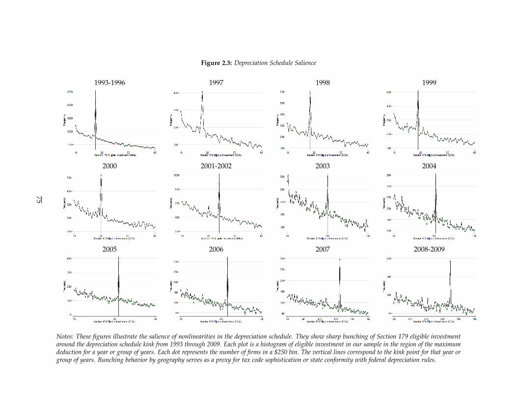
Figure 2.3: Depreciation Schedule Salience

1993-1996 1997 1998 1999

2000 2001-2002 2003 2004

2005 2006 2007 2008-2009

Notes: These figures illustrate the salience of nonlinearities in the depreciation schedule. They show sharp bunching of Section 179 eligible investmentaround the depreciation schedule kink from 1993 through 2009. Each plot is a histogram of eligible investment in our sample in the region of the maximumdeduction for a year or group of years. Each dot represents the number of firms in a $250 bin. The vertical lines correspond to the kink point for that year orgroup of years. Bunching behavior by geography serves as a proxy for tax code sophistication or state conformity with federal depreciation rules.

75

In general, evidence of bunching at kink points reflects a mix of reporting and real

responses.50 The bunching evidence is informative in either case because these are both

behavioral responses, which show whether firms understand and respond to the schedule.

In the next section, we study managerial myopia by comparing bunching activity across

different groups of firms. This test does not depend on whether the response is real or

reported.

We can interact the bunching evidence with the basic regression model identifying the

response to bonus. The design of the test generates control and treatment groups from the

notion that firms differ in their tax code knowhow.51 We compute geographic proxies of

investment schedule sophistication through measuring the local propensity to bunch at the

Section 179 kink point. We use the low information areas as cross-sectional counterfactuals

for the high information areas. We then separately estimate the baseline model for each

group, effectively providing a difference-in-difference-in-differences estimate of the bonus

response.

We group firms by two-digit ZIP code, which is the lowest level of aggregation that

permits a reliable measure of bunching. For each ZIP-2, we pool all years and compute the

fraction of firms within $10,000 of the kink who bunch within $250 of it. This provides the

sorting variable. In this design, more bunching in a region indicates more awareness of

the tax code for that region. So, we should expect the growth in investment during bonus

periods to be increasing in the level of bunching. Columns seven and eight of Table 2.4

50See Saez (2010) for a discussion of this point. The bonus difference-in-differences (DD) design is lessvulnerable to misreporting. In that design, we can confirm the response by looking at other outcomes. Inaddition, the DD estimator is much less sensitive to misreporting by a small fraction of total investment.Moreover, the sample contains many firms who use external auditors, for whom misreporting investmententails substantial risk and little benefit. Last, our conversations with tax preparers and corporate tax officerssuggest that misreporting investment is an inferior way to avoid taxes. This is because investment purchases aretypically easily verifiable, require receipts when audited, and usually reduce current taxable income by just afraction of each dollar claimed as spent. In the case of investment expenses depreciated over multiple years, theaudit risk of misreporting is also extended over the entire depreciation schedule.

51This test follows the design of Chetty, Friedman and Saez (2013), who use geographic differences inindividual bunching at a kink in the Earned Income Tax Credit schedule to study the labor supply response totaxes. An alternative explanation for the differences we observe is state differences in conformity with federalbonus rules (Kitchen and Knittel, 2011).

76

show that indeed the high bunching areas display a stronger response to bonus than do the

low bunching areas.52

Substitution Margins and External Finance. We ask whether increased investment in-

volves substitution away from payroll or equipment rentals, how firms finance their addi-

tional investment, and whether the increased investment reflects intertemporal substitution

or new investment. Understanding substitution margins is critical for assessing the macroe-

conomic impact of these policies and provides further indication of whether the observed

response is real. Studying external finance responses helps us understand how firms paid

for new investments.

Table 2.5 presents estimates of the intratemporal and intertemporal substitution margins.

These regressions follow the baseline specification in equation 2.4.1, with a different left

hand side variable. For rents, payroll and debt, we focus on flows (namely, differences in

logs) as outcomes that match investment most closely. For payouts, we study an indicator

for whether dividends are non-zero.

How flexible is the rent-versus-own margin for equipment investment? If firms simply

shift away from leasing to take advantage of the tax benefits of buying, then the aggregate

impact of these policies will be minimal. In their tax returns, firms separately report rental

payments for computing net income. Unfortunately, this item does not permit decomposition

into equipment and structures leasing. Acknowledging this limitation, we ask what effect

bonus depreciation had on changes in rental payments. The first column of Table 2.5 shows

that growth in rental payments did not slow due to bonus, but rather increased somewhat.

Thus we do not find evidence of substitution away from equipment leasing. The second

column of Table 2.5 reports the effect of bonus on growth in non-officer payrolls. Again, we

find no evidence of substitution, but rather coincident growth of payroll. Finding limited

substitution in both leasing and employment makes it more likely that bonus incentives

caused more output.

52Specifically, we compare the top and bottom three deciles of local bunching.

77

Table 2.5: Substitution Margins and External Finance

Dependent Variable

∆Rents ∆Payroll ∆Debt Payer? Investment

(1) (2) (3) (4) (5)

zN,t 0.75∗∗ 1.49∗∗∗ 1.84∗∗∗ -0.36∗∗∗ 4.22∗∗∗

(0.26) (0.20) (0.21) (0.089) (0.62)

zN,t−2 -0.86(0.69)

Observations 574305 624918 642546 818576 476734Clusters (Firms) 98443 102043 103868 128150 84777R2 0.18 0.23 0.20 0.68 0.76

Notes: This table estimates regressions of the form

Yit = αi + βzN,t + γXit + δt + εit

where Yit equals the difference in the logarithm of the dependent variable in columns (1) through (3). In column(4), the dependent variable is an indicator for positive dividend payments. zN,t is the present value of a dollarof eligible investment computed at the four-digit NAICS industry level, taking into account periods of bonusdepreciation. Column (5) includes contemporaneous and twice lagged zN,t. All regressions include firm andyear fixed effects. Standard errors clustered at the firm level are in parentheses.

While increased depreciation deductions do allow firms to reduce their tax bills and keep

more cash inside the firm, they must still raise adequate financing to make the purchases

in the first place. This point is especially critical if firms thought to be in tight financial

positions respond more. Here, we test whether bonus incentives affect net issuance of

debt and payout policy. Columns (3) and (4) of Table 2.5 provide some insight. Increased

equipment investment appears to coincide with significantly expanded borrowing and

reduced payouts.

We assess the extent of intertemporal substitution using a model that includes both

contemporaneous z and lagged z. In the case of temporary incentives, the shifting of

investment from the high tax future to the low tax present offers a potential source of

amplification (Abel, 1982; House and Shapiro, 2008). Our data often do not include the

fiscal year month, so it is possible that we are marking some years as t when they should be

t− 1 or t + 1. For most of our tests, this issue introduces an attenuation but no systematic

bias. However, when testing for intertemporal substitution, we want to be sure that lagged

78

z measures past policy changes. Thus column (6) of Table 2.5 includes regressions with

twice lagged z added to the baseline bonus model. The coefficient on lagged z is negative

but not distinguishable from zero and including lagged z does not alter the coefficient on

contemporaneous z. This implies limited intertemporal shifting of investment, which further

motivates our study of amplification through financial frictions.

Summary. Bonus depreciation has a large effect on investment, and spurious time-varying

industry factors cannot explain this fact. Such factors would cause parallel trends to fail

in the years prior to bonus. They would lead to different estimates in recessions marked

by weakness in different industries. They would lead ineligible investment to expand.

They would attenuate the estimated effect when regressions include flexible industry-by-

time controls. And they would lead to a similar response across geographies where firms

pay more and less attention to the depreciation schedule. The facts do not match these

predictions. Section 2.5, which presents heterogeneous effects by firm size and tax position,

further contradicts the omitted industry factor story.

These investment responses directly correspond to take-up of depreciation incentives—

bonus take-up rates rise with the policy’s generosity and many firms sharply bunch around

the Section 179 kink point—in contrast to recent work on partial salience of sales taxes

(Chetty, Looney and Kroft, 2009) and the nonresponse of investment to dividend tax changes

(Yagan, 2013). Net investment responds to bonus depreciation as well, even though the

reported balance sheet items do not affect taxable income. Debt issuance increases because

of bonus depreciation and payroll and dividend payments—which are double reported—

respond as well. Thus the observed response is a policy response that does not reflect a

mere reporting response, but rather reflects real economic behavior.

2.5 Explaining the Large Response with Financial Frictions

The large response of investment to bonus depreciation is not consistent with a frictionless

model of firm behavior: the magnitudes imply implausibly high discount rates. In this

79

section, we explore alternative models that can generate high effective discount rates and

thus reconcile our estimates with past work.

One alternative is costly external finance, which raises the total discount rate firms apply

to evaluate projects. Our rich data environment enables us to study how the investment

response to tax incentives interacts with costly external finance. We perform a series

of split sample tests, using several common markers of ex ante financial constraints.53

Consistent with this story, firms more likely to depend on costly external finance—small

firms, non-dividend payers and firms with low levels of cash—respond more strongly to

bonus.

Another alternative model is managerial myopia, which raises effective discount rates

by sharply discounting the future relative to the present. Consistent with this story, firms

only respond to investment incentives when the policy immediately generates after-tax cash

flows. For firms with positive taxable income before depreciation, expanding investment

reduces this year’s tax bill and returns extra cash to the firm today. Firms without this

immediate incentive can still carry forward the deductions incurred but must wait to receive

the tax benefits.54 We present evidence that, for both Section 179 and bonus depreciation,

this latter incentive is weak, and differences in growth opportunities cannot explain this

fact.

2.5.1 Heterogeneous Responses by Ex Ante Financial Constraints

We divide the sample along several markers of ex ante financial constraints used elsewhere

in the literature. Even for private unlisted firms, we can still measure size, payout frequency

and proxies for balance sheet strength. Panel (b) of Figure 2.2 plots elasticities and confidence

53See Fazzari, Hubbard and Petersen (1988a) for an early application of this methodology and Almeida,Campello and Weisbach (2004) and Chaney, Sraer and Thesmar (2012) for recent examples.

54In the code, current loss firms have the option to “carry back” losses against past taxable income. The IRSthen credits the firm with a tax refund. Our logic assumes that firms have limited loss carryback opportunitiesbecause, in the data, we find low take-up rates of carrybacks. Furthermore, carrybacks create a bias against ourfinding a difference between taxable and nontaxable firms, because carrybacks create immediate incentives forthe nontaxable group.

80

bands from regressions run for each of ten deciles based on average sales.55 The smallest

firms in the sample show the largest response to bonus. These estimates help us reconcile

our findings with past studies. Larger firms show user cost elasticities in line with the

findings surveyed in Hassett and Hubbard (2002). It is only the smaller firms, for whom

data were previously unavailable, that yield estimates outside the consensus range.

Table 2.6 presents a statistical test of the difference in elasticities across three markers

of ex ante constraints. For the sales regressions, we split the sample into deciles based

on average sales and compare the bottom three to the top three deciles.56 The average

semi-elasticity for small firms is twice that for large firms and statistically significantly

different with a p-value of 0.03.57 The second two columns present separate estimates

for firms who paid a dividend in any of the three years prior to the first round of bonus

depreciation.58 The non-paying firms are significantly more responsive.

Our third sample split is based on whether firms enter the bonus period with relatively

low levels of liquid assets. We run a regression of liquid assets on a ten-piece linear spline

in total assets plus fixed effects for four-digit industry, time, and corporate form. We sort

firm-year observations based on the residuals from this regression lagged by one year,

and then report in the last two columns of Table 2.6 separate estimates for the top and

bottom three deciles. Note that this sort is uncorrelated with firm size by construction. The

estimates are reported in the last two columns of Table 2.6. The results using this marker of

liquidity parallel those in the size and dividend tests, with the low liquidity firms yielding

an estimate of 7.2 as compared to 2.8 for the high liquidity firms.

55Specifically, we use average sales from the three years before each bonus period. We use as many of thesesix years as are available for each firm.

56When we measure size with total assets or payroll, the size results are unchanged.

57Cross equation tests are based on seemingly unrelated regressions with a variance-covariance matrixclustered at the firm level.

58We only use the first round of bonus for the dividend split. The dividend tax cut of 2003, which had astrong effect on corporate payouts (Yagan, 2013), may have influenced the stability of this marker for the laterperiod.

81

Table 2.6: Heterogeneity by Ex Ante Constraints

Sales Div Payer? Lagged Cash

Small Big No Yes Low High

zN,t 6.29∗∗∗ 3.22∗∗∗ 5.98∗∗∗ 3.67∗∗∗ 7.21∗∗∗ 2.76∗∗

(1.21) (0.76) (0.88) (0.97) (1.38) (0.88)

Equality Test p = .030 p = .079 p = .000

Observations 177620 255266 274809 127523 176893 180933Clusters (Firms) 29618 29637 39195 12543 45824 48936R2 0.44 0.76 0.69 0.80 0.81 0.76

Notes: This table estimates regressions from the baseline intensive margin specification presented in Table 2.3.We split the sample based on pre-policy markers of financial constraints. For the size splits, we divide thesample into deciles based on the mean value of sales, with the mean taken over years 1998 through 2000. Smallfirms fall into the bottom three deciles and big firms fall into the top three deciles. For the dividend payer split,we divide the sample based on whether the firm paid a dividend in any of the three years from 1998 through2000. The dividend split only includes C corporations. The lagged cash split is based on lagged residuals from aregression of liquid assets on a ten piece spline in total assets and fixed effects for four-digit industry, year andcorporate form. The comparison is between the top three and bottom three deciles of these lagged residuals. Allregressions include firm and year fixed effects. Standard errors clustered at the firm level are in parentheses.

These constraint markers are imperfect.59 First, they do not directly measure the external

finance cost faced by new firms. This concern would tend to bias any differences existing

between groups toward zero, and thus against the results we present. A second concern

with sample splitting is that the splitting criteria are correlated with the investment error

term and so may bias the estimated coefficient of interest (Bond and Van Reenen, 2007).

This issue is important for investment-cash flow sensitivity tests because cash flow is likely

correlated with other components of the investment error term. Because our setting features

plausibly exogenous policy variation at the industry level, this concern is less important

here. The key assumption we make is that interacting our splitting criterion, measured

prior to the policy change, with the policy variable and the year effects enables a valid

difference-in-differences design for each group.

59Criticism of split sample markers dates back to Poterba’s comments in Fazzari, Hubbard and Petersen(1988a). See Farre-Mensa and Ljungqvist (2013) for a more recent assessment of their value in samples of publicand private companies.

82

2.5.2 Heterogeneous Responses by Tax Position

The Section 179 bunching environment offers an ideal setting for documenting the immedi-

acy of investment responses to depreciation incentives. The simple idea is to separate firms

based on whether their investment decisions will fully offset current year taxable income, or

whether deductions will have to be carried forward to future years. We choose net income

before depreciation expense as our sorting variable. Firms for which this variable is positive

have an immediate incentive to invest and reduce their current tax bill. If firms for which

this variable is negative show an attenuated investment response and these groups are

sufficiently similar, we can infer that the immediate benefit accounts for this difference.

The panels of Figure 2.4 starkly confirm this intuition. In Panel (a), we pool all years

in the sample, recenter eligible investment around the year’s respective kink, and split

the sample according to a firm’s taxable status. Firms in the left graph have positive net

income before depreciation and firms in the right graph have negative net income before

depreciation. For firms below the kink on the left, a dollar of Section 179 spending reduces

taxable income by a dollar in the current year. Retiming investment from the beginning of

next fiscal year to the end of the current fiscal year can have a large and immediate effect on

the firm’s tax liability. For firms below the kink on the right, the incentive is weaker because

the deduction only adds to current year losses, deferring recognition of this deduction until

future profitable years. As the figure demonstrates, firms with the immediate incentive to

bunch do so dramatically, while firms with the weaker, forward-looking incentive do not

bunch at all.60

One objection to the taxable versus nontaxable split is that nontaxable firms have poor

growth opportunities and so are not comparable to taxable firms. We address this objection

in two ways. First, we restrict the sample to firms very near the zero net income before

depreciation threshold to see whether the difference persists when we exclude firms with

large losses. Panel (a) of Appendix Figure B.1 plots bunch ratios for taxable and nontaxable

60On average, half of the nontaxable firms transition to taxable status in the next year. Thus this providesfurther evidence against amplification through intertemporal substitution, in which nontaxable firms expectinghigher future taxes should also respond.

83

Figure 2.4: Bunching Behavior and Tax Incentives

(a) By Current Year Tax Status (b) By Lagged Loss Carryforward Stock

0

5000

−10 −5 0 5 10 −10 −5 0 5 10

Net Income Plus Depreciation >= 0 Net Income Plus Depreciation < 0

Num

ber

of F

irms

Section 179 Eligible Investment Around Cutoff (000s)Graphs by loss

Notes: These figures illustrate how bunching behavior responds to tax incentives. Firms bunch less wheneligible investment provides less cash back now. Panel (a) splits the sample based on whether firm net incomebefore depreciation is greater than or less than zero. Firms with net income before depreciation less than zero cancarry back or forward deductions from eligible investment but have no more current taxable income to shield.Panel (b) groups firms with current year taxable income based on the size of their prior loss carryforward stocks.The x-axis measures increasing loss carryforward stocks relative to current year income. The y-axis measuresthe excess mass at the kink point for that group. Firms with more alternative tax shields find investment a lessuseful tax shield and therefore bunch less.

84

firms, estimated within a narrow bandwidth of the tax status threshold. The difference in

bunching appears almost immediately away from zero, with the confidence bands separating

after we include firms within $50 thousand dollars of the threshold. For loss firms, the

observed pattern cannot be distinguished from a smooth distribution, even for firms very

close to positive tax position. The bunching difference for nontaxable firms is not driven by

firms making very large losses.

Table 2.7 replicates the tax status split idea in the context of bonus depreciation. We

modify the intensive margin model from Table 2.3 by interacting all variables with a

taxable indicator based on whether net income before depreciation is positive or negative.61

According to these regressions and consistent with bunching results, the positive effect of

bonus depreciation on investment is concentrated exclusively among taxable firms. The

semi-elasticity is statistically indistinguishable from zero for nontaxable firms, while it is 3.8

for taxable firms. In Panel (b) of Appendix Figure B.1, we repeat the narrow bandwidth test

for bonus depreciation. The figure plots the coefficients on the interaction of taxable and

nontaxable status with the policy variable. The difference in coefficients in Table 2.7 emerges

within $50 thousand of the tax status threshold, and these coefficients are statistically

distinguishable within $100 thousand of the threshold. Here as well, the results are not

driven by differences for firms far from positive tax positions.

To further address the concern about nontaxable firms, Panel (b) of Figure 2.4 uses

differences within the group of taxable firms. This plot shows again that bunching is due to

tax planning with regard to the immediate potential benefit. Here, we divide profitable firms

by their stock of loss carryforwards in the previous year. Each dot in this plot represents a

bunching histogram where the y-axis measures the degree of bunching using the excess

mass estimator in Chetty et al. (2011). The groups are sorted according to the ratio of lagged

loss carryforward stock to current year net income before depreciation, which proxies for

the availability of alternative tax shields. The scatter clearly indicates a negative relationship

61That is, we interact z, any controls, and the time fixed effects with the taxable indicator. We do not interactthe firm effects with the taxable indicator.

85

Table 2.7: Heterogeneity by Tax Position

LHS Variable is Log(Investment)

(1) (2) (3) (4) (5) (6) (7)

Taxable 3.83∗∗∗ 3.08∗∗∗ 1.95∗ 6.43∗∗∗ 4.32∗∗∗ 4.15∗∗∗

× zN,t (0.79) (0.93) (0.92) (1.46) (0.96) (0.82)

zN,t -0.15 0.60 0.38 -3.03∗ -0.69 0.88 5.68∗∗∗

(0.90) (1.05) (1.06) (1.55) (1.15) (0.94) (1.70)

Medium LCF -2.56× zN,t (1.46)

High LCF -3.70∗

× zN,t (1.55)

CFit/Ki,t−1 0.14∗∗∗

(0.028)

Taxable 0.27∗∗∗

× CFit/Ki,t−1 (0.035)

Observations 735341 580422 514035 221306 585914 722262 119628Clusters (Firms) 128001 100883 109678 63699 107985 124962 40282R2 0.71 0.74 0.74 0.80 0.73 0.72 0.84

Controls No No No No Yes No NoIndustry Trends No No No No No Yes No

Notes: This table estimates regressions from each intensive margin in columns (1) through (6) specificationpresented in Table 2.3. For each firm year, we generate an indicator based on whether a firm is in taxableposition prior to depreciation expense. We fully interact this indicator with all controls and the time effects.Column (7) splits taxable firms into three groups based on the size of their lagged loss carryforward stocksrelative to net income before depreciation. We interact these group indicators with zN,t and the time effects.Only firms with nonzero stocks of lagged loss carryforwards are included. All regressions include firm andyear fixed effects. Standard errors clustered at the firm level are in parentheses.

86

between the presence of this alternative tax shield and the extent of eligible investment

manipulation.

We confirm this pattern in the bonus setting. Column (7) of Table 2.7 focuses on the

group of taxable firms with non-zero stocks of lagged loss carryforwards. We split this

group into three subgroups based on the size of their carryforward stock. Firms with large

stocks of loss carryforwards display a semi-elasticity with respect to z of 2 compared to a

semi-elasticity of 5.7 for firms with low loss carryforward stocks.

The finding for nontaxable firms contradicts a simple model of costly external finance,

because firms neglect how the policy affects borrowing in the future. On the other hand,

firms cannot be too myopic because the investment decision itself only pays off in the future.

Thus for myopia to be the explanation, firms must use different accounts to think about

investment decisions and the tax implications. Moreover, the myopia story must also explain

the finding for financially constrained firms—are small firms, non-dividend payers and

firms with low levels of cash more myopic?

The facts presented in this section—the stronger response for financially constrained

firms and the nonresponse for nontaxable firms—do not match the predictions of a friction-

less model. The facts point instead toward models in which costly external finance matters

and current benefits outweigh future benefits, with neither alternative being obviously

redundant.

2.5.3 Discount Rates and the Shadow Cost of Funds

Taken together, our empirical findings emphasize a financial frictions channel for how

investment incentives work. We use a standard investment model to quantify the importance

of this channel. Specifically, we ask what is the marginal value of cash, λ, implied by our

financial constraint split sample analysis, and what is the discount term, β, implied by our

tax status split sample analysis. The answers allow us to summarize our findings through

an implied discount rate that firms seem to apply in evaluating investment incentives.

In Appendix Section B.1, we derive the comparative static for investment with respect to

87

the bonus depreciation term θ:

I · ε I,θ ≡∂I∂θ

=(1 + λ)pI

ψI I

∂z∂θ

> 0 (2.5.1)

where ε I,θ is the semi-elasticity of investment with respect to θ, pI is the price of investment,

ψI I is the second derivative of the adjustment cost function, and z is defined as in (2.2.3).

In the Appendix, we state assumptions under which I · ψI I will be equal across groups.62

Under these assumptions, we can derive two empirical moments that combine our estimates

for constrained and unconstrained firms and for taxable and nontaxable firms and yield

simple formulas for λ and β.

The first empirical moment we use compares the estimated response with respect to

bonus for constrained and unconstrained firms. Assuming constrained firms face shadow

price λC and unconstrained firms face shadow price λU , we take the ratio of comparative

statics:εC

I,z

εUI,z≡ m1 =

∂I/∂θ|λC

∂I/∂θ|λU

=1 + λC

1 + λU= 1 +

∆λ

1 + λU, (2.5.2)

which reveals an implied credit spread between constrained and unconstrained firms. Table

2.8 presents m1 for each pair of estimates in Table 2.6. λ is the shadow price of relaxing the

firm’s borrowing constraint. An alternative interpretation is that every after-tax dollar inside

the firm is worth 1 + λ dollars outside the firm. Our estimates reveal that, for financially

constrained firms, a dollar inside the firm is worth $2.06 on average outside the firm.

Is this estimate reasonable? There are not many existing benchmarks. Faulkender and

Wang (2006) attempt a calculation with a very different methodology, but that ultimately

arrives at a similar conclusion. They estimate the value of changes in cash in excess return

regressions, while attempting to control for a host of omitted factors. They find that for low

payout firms and for small firms the value of a dollar of after-tax cash is worth $1.67 and

$1.62, respectively. For these firms’ unconstrained counterparts, a dollar is only worth $1.07

and $1.12. The spreads in their study are comparable to ours, especially considering their

62That is, we assume linear homogeneity of the marginal adjustment cost function. Nearly all studies in theliterature make this assumption, which is necessary for example for marginal q to equal average Q.

88

Table 2.8: Calibrated Moments

Shadow Cost of Funds Calibration

Mean Sales Dividend Payers Lagged Cash Average

m1 1.95 1.63 2.61 2.06λC|λU=0 0.95 0.63 1.61 1.06

Discount Factor Calibration

p φ r β

High φ 0.51 0.88 0.07 0.82Medium φ 0.31 0.82 0.07 0.84Low φ 0.05 0.42 0.07 0.97

Notes: This table computes empirical estimates for m1 and m2, as defined in the text. m1 reveals an impliedcredit spread between constrained and unconstrained firms. m2 reveals the discount factor firms apply to allfuture cash flows relative to current flows.

exercise operates within a group of firms we consider to be relatively unconstrained.63

We define a second empirical moment that compares taxable and nontaxable firms:

εγ=0I,z

εγ=1I,z

≡ m2 =∂I/∂θ|γ=0

∂I/∂θ|γ=1= βφ

1− z0t (1)

1− z0t (β)

(2.5.3)

where φ is a discounter that reflects the average arrival of the taxable status event for

nontaxable firms. We proxy for φ by assuming a fixed transition probability p for nontaxable

firms and an infinite horizon for realizing carryforwards.64 This implies φ = p/(p+ r).65 We

calibrate p using tax status transitions in the data. Specifically, we measure the probability

that a currently nontaxable firm has sufficient income in the next year for depreciation

deductions to affect next year’s tax bill. In our data, this probability is 0.51 if future loss

carryforwards are not used and 0.31 if all future carryforwards are deducted prior to

63Similarly, Koijen and Yogo (2012) find that a relaxed borrowing constraint for life insurers during thefinancial crisis is worth $2.32 per dollar of inside capital.

64The actual expiration period for carryforwards is twenty years.

65That is, the expected arrival is p/(1 + r) + (1− p)p(1 + r)−2 + (1− p)2 p(1 + r)−3 + · · · = p/(1 + r) ·[1/(1− (1− p)/(1 + r))] = p/(p + r).

89

considering investment incentives.66 We also consider an extreme transition probability of

0.05.

Note the external finance wedge falls out of this expression. This is true as long as

average shadow costs are the same across taxable and nontaxable groups. To maintain this

assumption, we use our loss carryforward group estimates to calibrate m2. That is, we

estimate semi-elasticities within the group of taxable firms sorted according to their past

stocks of alternative tax shields. For firms with large loss carryforward stocks relative to

current income, the marginal dollar of investment is unlikely to affect this year’s tax bill. At

the same time, we have less reason to believe these firms face substantially worse growth

opportunities or tighter financial constraints. This biases our estimates of β toward the

neoclassical benchmark of β equal to one.

Applying the estimates from the last column of Table 2.7 yields a value for m2 of

0.35(= (5.68− 3.7)/5.68). For p = 0.51, this maps to an implied discount factor (β) of

0.82.67 The more conservative p = 0.31 hardly affects the calculation; only a counterfactual,

extreme expectation of loss persistence can justify a β near the neoclassical benchmark.

Ignoring for the moment the other discount terms, β equal to 0.82 implies a discount rate of

approximately 20 percent. We are not aware of studies that attempt to measure discount

factors such as this for firms. Prior studies on individual decision making have found

similar magnitudes for short term discount rates in both lab and field experiments.68

The discounting implied by β says that one dollar next year is worth 82 cents, before

taking into account risk or the shadow cost of funds. If we then apply the assumed risk

adjusted rate of 7 percent and the estimated shadow cost of funds of 1.06, we find that

a dollar next year is worth approximately 38 cents today for the financially constrained

66Auerbach and Poterba (1987b) note more persistence of nontaxable positions than we do. Our measure isbased on net income before depreciation, to capture the state of having the next dollar of investment affect thisyear’s tax bill. Their measure is based on whether firms exhaust their carryforward stocks.

67We evaluate z0t (1) at the sample average of 0.88 and use the sample average first year deduction of 0.18 to

set z0t (β) = 0.18 + β× 0.7.

68Laibson D. Repetto and Tobacman (2007) estimate short term discount rates of 40 percent in the context ofindividual saving decisions. In a more general model, they estimate a short run discount rate of 15 percent anda long run rate of 3 percent.

90

firms in our sample. This substantial discount is not surprising, given the starkness of

the reduced form empirical results: nontaxable firms seem to ignore the future benefits

and small, financially constrained firms seem to value highly the immediate cash back

due to bonus depreciation. In the model, we use costly external finance and myopia to

describe the observed deviations from a rational benchmark, but the exercise performed

here provides just one of several plausible calibrations of this basic fact. In general, models

of firm behavior that do not generate high discount rates are unlikely to fit the data for most

firms.

2.6 Conclusion

This paper combines methods from public and applied economics with insights from

finance to answer a first order macroeconomic question: how do taxes affect investment

behavior in the presence of financial frictions? We find that firms respond strongly to

incentives that directly target investment decisions. Our heterogeneity results—that the

investment response is larger for financially constrained firms, but only when the benefit is

immediate—show that financial frictions are critical for understanding investment behavior.

The results point toward a set of models in which costly external finance matters and

firms place more weight on current benefits than they would in a frictionless model. Whether

the high implied discount rate reflects an external finance wedge, managerial myopia, agency

considerations or a mix of these is an important question for future research. Further study

of the external finance mechanism would be valuable. A deeper study of the employment

effects of these policies is of direct interest to macroeconomists and policymakers.

A related question for future research concerns the effects of tax planning. How do tax

preparers affect the decision to take up these policies? More generally, do firms focus on

minimizing current taxes at the possible expense of future payoffs? The answer to these

questions might shed light on the role of agency problems and firm learning about optimal

management practices.

The empirical results imply that policies which target investment directly and yield

91

immediate payoffs are most likely to influence investment activity. Policies that target

financial constraints, such as direct loans, might have a similar effect if conditional on the

investment decision. In comparison to studies of consumer durable goods, we find less

evidence of intertemporal shifting, but more work on this question is needed. Data from the

period following the recent stimulus, once available, will be very useful.

92

Chapter 3

Do the Victors Share the Spoils?

Evidence from US House Elections,

1982-2006

3.1 Introduction

How does US congressional politics affect the distribution of federal spending across

voters? A substantial body of research has focused on which legislators receive more

spending for their districts, but less is known about the allocation of federal spending across

constituents within districts. Theoretical models of elections where candidates propose

spending allocations across a distribution of voters on a left-right ideological dimension

make competing predictions over whether swing, co-partisan, or both types of voters will

benefit disproportionately. I test between these models within a sub-sample of congressional

districts from the US House of Representatives by measuring the within-district distribution

of per-capita federal spending across counties. I find that neither counties with co-partisan

voters nor swing voters receive disproportionately more spending.

Much of the distributive politics literature of US federal spending has focused on which

legislators receive the most spending for their districts. Theoretically, legislative bargaining

93

models have explored how recognition rules among legislators affect the equilibrium

distribution of benefits when legislators engage in repeated rounds of voting over proposed

spending allocations (Baron and Ferejohn 1989, McCarty 2000, McKelvey and Riezman 1992).

In these models, the first legislator recognized to propose an allocation has an advantage

due to the costs of legislative delay. Consequently, the empirical literature has measured how

predictors of legislator proposal power affect the distribution of US federal spending across

congressional districts and states, such as partisan alignment with congressional majorities

(Albouy 2013, Balla et al. 2002, Bickers and Stein 2000) and the president (Berry, Burden and

Howell 2010, Larcinese, Rizzo and Testa 2006), congressional committees (Alvarez and Lowry

1997, Carsey and Rundquist 1999, Ferejohn 1974, Heitshusen 2001, Levitt and Poterba 1999,

Knight 2005), and bicameralism (Lauderdale 2008, Shepsle et al. 2009). Most recently, Berry,

Burden and Howell (2010) finds larger effects for partisan alignment than congressional

committees on the distribution of federal spending aggregates across congressional districts.

All of these studies assume that legislators want to capture federal spending for their

constituents, but how should they distribute that spending among their constituents? Are

all constituents political equals? A theoretical literature in distributive politics considers this

question in the context of two-candidate elections. When voters differ in their ideological

orientation on a left-right dimension, alternative models make competing predictions for

whether candidates propose spending allocations that disproportionately benefit co-partisan

or swing voters (Dixit and Londregan 1996, Hirano, Snyder and Ting 2009, Lindbeck and

Weibull 1987). By comparing the within-district distribution of spending and voting patterns

across counties, my empirical exercise tests whether the predictions from those models bear

out in meaningful ways for federal spending aggregates in the context of the US House of

Representatives.

Within individual congressional districts and each Congress, I estimate the difference in

per-capita federal spending across counties using a 26-year panel for a range of spending

measures. Although legislators could use geography and demography in a variety of

94

strategies to target federal spending to specific groups of voters,1 there is a substantial

amount of spending that they are unlikely to manipulate for this purpose, such as broad-

based entitlement programs. I thus report results for a range of spending measures from

broad aggregates to place-specific grants and contracts to manage this trade-off between

broad and manipulable spending. In the discussion of my results that follow, I will focus

on my non-entitlement measure which excludes the largest entitlement programs, Social

Security, Medicare, and Medicaid, from the total spending measure.

To characterize the distribution of spending within congressional districts, I use a

rural sub-sample of districts because I can only reliably measure broad aggregates of

federal spending at the county-level and many urban counties are split across multiple

congressional districts. Largely because I exclude districts that do not entirely contain at

least three counties, my sample includes about 39 percent of all congressional districts.2

While my main estimates are representative for a rural sub-sample of US congressional

districts, the same electoral pressures that motivate the distributive politics models that I

test are present in both rural and urban districts. Furthermore, I replicate my tests when

possible in the context of the US Senate where I can include urban counties.

For the within-district distribution of voters, I define partisan county quantiles using the

county mean and standard deviation of the Republican vote share in presidential elections

across the entire panel. Counties are defined as either co-partisan or opposition and as

either swing or base. Intuitively, these relative within-district measures define counties as

co-partisan when they tend to vote for the winning candidate’s party and as swing when

their Republican vote share exhibits greater variability from election to election.3 While

spending may be targeted to voters at a narrower geographic level, the per-capita county

1For example, programs such as low-income housing and agricultural subsidies that are allocated by formulacan provide benefits to specific demographic groups. Alternatively, grants and contracts such as academicresearch awards or bridge construction can be allocated to specific places.

2Figure 3.1 presents two maps that depict my sample for the 98th and 110th Congresses.

3Within individual congressional districts and each Congress, I evenly divide all counties into Republicanand Democratic halves using the panel mean, and into swing and base halves using the panel standard deviationof the Republican vote share in presidential elections. Then, I define counties as co-partisan when they sharethe same partisanship as their House representative and conversely for opposition counties.

95

means should reflect any bias in the aggregate distribution of spending across voters.

For my main results, I estimate differences in per-capita federal spending between

partisan county quantiles within congressional districts of the US House of Representatives.

My specifications include district-congress4 fixed effects to focus on the relative allocation

of spending across counties within each district-congress. I also include county fixed effects

to absorb county-level spending that is unrelated to changes in the political environment.

In this framework, my estimates of the differences between counties within each district

are identified from party switches in elections and redistricting. Party switches allow me

to identify the effect for co-partisan counties because the two parties have different core

supporters. It cannot, however, identify the effect for swing counties because both parties

have the same swing voters. Because redistricting changes the composition of counties

within districts, I can use it to identify both co-partisan and swing counties as the partisan

county quantiles are relative definitions among the counties within each district-congress.

I report results from three alternative strategies to estimate the within-district differences

across counties. In all cases, I find reasonably precise null effects. First, I estimate the

differences in log per-capita spending across partisan county quantiles in the full panel,

including district-congress and county fixed effects as described above. Second, I implement

a regression discontinuity design (RDD) on two-party elections in order to address concerns

that congressional districts where Republicans and Democrats are elected may differ in

important ways that also affect their within-district distribution of spending. Because this

method relies on party switches, it can only identify the co-partisan counties. Third, I

report first-difference estimates where I restrict the sample to the periods before and after

redistricting where the party of the House representative also remains unchanged. Here, I

isolate redistricting as the source of identification and focus on its immediate impact on the

within-district distribution of spending.

For the non-entitlement measure using the full panel, I find a point estimate of −0.0064

with a standard error of 0.0091 for the co-partisan county and a point estimate of 0.0003 with

4Unique pair of congressional district and biannual Congress.

96

a standard error of 0.0158 for the swing county. To place these magnitudes in perspective,

Berry, Burden and Howell (2010) finds a point estimate of 0.040 for the effect of a partisan

match between a House representative and the president on a district’s log federal spending

in their most basic specification. Using their estimate as a baseline, I find magnitudes that are

16 percent and 0.75 percent as large. Furthermore, the estimates from the three methods that

I implement respectively allow me to rule out differences in per-capita spending between

co-partisan counties and base opposition counties greater than 1.1, 3.5, and 0.2 percentage

points5 under a 95 percent confidence interval. Similarly, I can rule out differences between

swing counties and base opposition counties greater than 3.1 and 3.3 percentage points

from the full panel and first-difference estimates.

While I find a flat distribution of spending across counties for a sub-sample of congres-

sional districts, my results could be criticized for largely excluding urban districts if the

greater overall levels of federal spending received by urban areas present more opportunities

for political manipulation. Furthermore, my results could mask heterogeneous treatment

effects if the capacity of House representatives to influence federal spending depends on

the cooperation of other political actors or legislative seniority. In particular, previous

papers find that partisan alignment increases overall levels of federal spending received by

congressional districts and states (Albouy 2013, Berry, Burden and Howell 2010, Larcinese,

Rizzo and Testa 2006). To address these concerns, I replicate the full panel estimates within

the context of the US Senate, where I can include urban counties, and with interactions for

partisan alignment with the House majority and the president, congressional committee

assignments, and the bicameral nesting of House and Senate districts in the US Congress.

These considerations do not substantively change my main results.

Within my sub-sample of congressional districts, I find limited evidence of substantial

distortions to the within-district distribution of federal spending aggregates that favors

broad groups of voters for electoral purposes. This result holds even when focusing on the

most influential House representatives. None of the standard two-candidate distributive

5Small differences in log points approximate differences in percentage points.

97

politics models with ideologically heterogeneous voters predict this flat within-district

distribution of spending across counties.6 The existing literature provides at least three

suggestions to understand this result. First, legislators may have chosen to adopt checks and

balances in the federal budget process to prevent themselves from biasing spending toward

one group of voters over another. Although individually preferable, the aggregate welfare

cost from this behavior may be so great that legislators commit themselves to preventive

procedures. Second, narrow self-interest may not guide voting behavior. The negligible

probability that voters have of being pivotal in an election suggest that no one would vote

purely on instrumental grounds. Third, voters may have imperfect information about the

distribution of federal spending. If poorly informed, they may neither be able to effectively

reward nor punish House representatives on this basis in elections. Instead, legislators may

focus on funneling concentrated benefits to well-informed special interests.

Within the US House of Representatives, this paper is the first to my knowledge that

tests two-candidate election models of distributive politics. While Berry, Burden and Howell

(2010) and Martin (2003) have constructed similar data sets matching county-level federal

spending to congressional districts, those papers do not capture the relative distribution

of spending and voters within each district because they do not include district-congress

fixed effects. Outside of the congressional context, Ansolabehere and Snyder (2006) have

implemented a similar design to look at the effect of party control of US State governments

on the county share of federal transfers to the state government. They find evidence that

co-partisan counties receiving greater spending levels, but not swing counties.

My findings also complement previous research about the distribution of spending and

voters across the United States from the perspective of the president and political parties

(Larcinese, Rizzo and Testa 2006, Larcinese, Snyder and Testa 2013, Levitt and Snyder

1995). While these papers present valuable empirical facts, my context of US congressional

districts provides more opportunities for causal inference. In this setting, I am able to

6Assuming an ideologically homogeneous set of voters, Myerson (1993) and Laslier and Picard (2002) findconditions under which two-candidate electoral competition results in uniform or near uniform balanced-budgetproposals across voters.

98

implement a RDD on two-party elections and a first-differences design on redistricting.

Furthermore, the two-candidate distributive politics models do not exactly apply to their

empirical setting because the winner-takes-all feature of the electoral college and legislator

districts changes the incentives faced by presidential candidates and political parties. In

particular, an additional vote in a safe state does not increase a presidential candidate’s

count in the electoral college in presidential elections. Examining the distribution of federal

spending within congressional districts allows for more plausibly causal estimates and more

direct testing of the two-candidate distributive politics models.

This paper proceeds as follows: Section 3.2 reviews predictions from the theoretical

distributive politics literature on the incentives that two-candidate elections create for

legislators in allocating spending across voters. Section 3.3 describes in greater detail the

panel construction and discusses some descriptive statistics. Section 3.4 presents my main

results for the full panel, RDD, and first-difference estimates. Section 3.5 presents my

robustness checks for the US Senate, partisan alignment, congressional committees, and

bicameralism. Section 3.6 concludes.

3.2 Motivation

In two-candidate election models of distributive politics, candidates compete over a distribu-

tion of voters on a left-right dimension by proposing alternative spending allocations across

voters under a balanced-budget rule. Voters then select a candidate on the basis of their

ideological tastes and the spending allocation promised to them. Whether co-partisan or

swing voters disproportionately benefit from candidate proposals depends on the model

set-up. In their most basic setting, Lindbeck and Weibull (1987) find that both candidates

will propose identical, uni-modal spending programs that disproportionately benefit swing

voters because they are ideologically indifferent between the two candidates. In contrast,

Dixit and Londregan (1996) find that co-partisan voters benefit disproportionately when

they assume that candidates are better at delivering the spending programs preferred by

their co-partisans. Ongoing political machines with a standing network of beneficiaries

99

could motivate this assumption, or alternatively candidates may have a better understanding

of the preferences of their co-partisans. Hirano, Snyder and Ting (2009)consider another

wrinkle by adding primary elections and forward-looking voters to the basic set-up. They

find that candidates will target both co-partisan and swing voters with spending because

primary voters elect candidates who (i) promise them spending and (ii) can win general

elections. Exploiting these conflicting predictions, I propose to test which of these models is

most empirically relevant for the distribution of federal spending within a sub-sample of

congressional districts.

In particular, I measure the per-capita distribution of federal spending across partisan

county quantiles defined in order to capture the sub-areas of each congressional district

with relatively high shares of co-partisan and swing voters. To limit endogeneity concerns

about voting behavior responding to spending patterns within congressional districts, I use

returns from presidential elections averaged over the entire panel. Using the panel mean

and the panel standard deviation of the presidential Republican vote share, I respectively

evenly sort counties into Republican and Democratic halves and into base and swing halves

within each district-congress. Then, I identify counties as co-partisan when they share the

same partisanship as their House representative and conversely for opposition counties.7

Intuitively, co-partisan counties have vote shares that tend to favor the party of the winning

candidate and swing counties have vote shares that vary from election to election, relative

to the other counties within their district-congress. While this paper focuses on estimates

that use this definition for the partisan county quantiles, I find similar results when I

consider three alternatives in Appendix Section C.3 based on House elections and on a

rolling window that excludes the concurrent election.8

With equation 3.2.1, I characterize the within-district distribution of spending across

7This procedure results in four types of counties: base co-partisan, swing co-partisan, swing opposition,and base opposition.

8Appendix Section C.3 replicates my main analysis using three alternative vote share statistics to definepartisan county quantiles: moving statistics from presidential elections, panel statistics from House elections,and moving statistics from House elections. The two moving statistics include the three previous presidentialelections and the five previous House elections respectively. Both exclude the concurrent election.

100

partisan county quantiles:

log (spendingcdt) = β1co-partisan countycdt + β2swing countycdt

+β3 (co-partisan countycdt × swing countycdt) + δc + ξdt + εcdt

(3.2.1)

where opposition county and base county are the omitted categories, δc is a fixed effect for

county c, and ξdt is a fixed effect for district d-congress t. Equation 3.2.1 includes district-

congress fixed effects to focus on the relative distribution of spending across counties

within each district-congress. The county fixed effects absorb county-level spending that

is unrelated to changes in the political environment. I also include an interaction between

co-partisan and swing counties to allow for the possibility that spending in these counties,

such as on local public goods, has more political value than if it only had relatively large

numbers of one or the other voter type. In this specification, the variation that identifies

the coefficients β1, β2, and β3 are switches in the party of the House representative and

redistricting that changes the collection of counties in the district. Using the log of spending,

the coefficients can also be interpreted as percentage point differences with the omitted

categories.

Assuming that the partisan county quantiles identify the counties with relatively high

shares of co-partisan and swing voters, the alternative distributive politics models make

competing predictions about the signs of the coefficients in equation 3.2.1. The basic model

in Lindbeck and Weibull (1987) predicts that β1 = 0, β2 > 0 and β3 = 0 because it finds that

both parties disproportionately reward swing voters. Dixit and Londregan (1996) predict

that β1 > 0, β2 = 0, and β3 = 0 when they assume that each party has an advantage in

targeting their own co-partisans. Hirano, Snyder and Ting (2009) predict that β1 > 0, β2 > 0,

and β3 > 0 because, while primary voters want spending for themselves, they also want

spending for swing voters in order to ensure winning the general election.

In addition to estimating equation 3.2.1, I also implement (i) a RDD on two-party

elections and (ii) a first-differences version of equation 3.2.1 on a sample limited to the

periods before and after redistricting where the party of the House representative also

101

remains unchanged. I use the RDD to address concerns that Republicans and Democrats

may get elected to congressional districts where the within-district distribution of spending

differs for reasons other than politics. With a first-differences approach, I can focus on the

immediate impact of redistricting and provide estimates less subject to long-term time-series

confounds.

While the theoretical distributive politics literature makes competing predictions about

the results that I should find, my test does not capture all the ways in which House

representatives could target spending to particular constituents. First, politicians may target

constituents very narrowly, such as key interest groups or large donors, instead of the broad

distribution of voters. Second, politicians may respond to voter preferences over the type of

spending, which may or may not have a geographic incidence that matches the distribution

of voters.9 Third, my identification strategies do not distinguish between whether the

spending allocation is determined by electoral incentives or by politician preferences. But

despite these limitations, my empirical exercise reveals whether the within-district patterns

of broad aggregates of federal spending across counties matches the predictions from the

two-candidate distributive politics models.

3.3 Data and descriptive statistics

3.3.1 US counties panel

The panel for this paper matches 1982-2006 US House elections to 1984-2009 county-level

federal spending measures. It is indexed by biannual Congresses from the 98th to the 110th

US Congress. Elections and federal spending have this staggered match because elections

take place the November before a new Congress starts and each congressional session passes

annual appropriations legislation for the following fiscal year.10 I also digitized biannual

9Albouy (2013), for example, finds that Republican legislators tend to receive more defense spending andDemocratic legislators tend to receive more education and housing and urban development spending for theirdistricts.

10Annual appropriations acts include a small number of multi-year appropriations. For acts passed in theyears 1995-2003, multi-year appropriation amounts accounted on average for 6.1 percent of the net total (Senate

102

congressional district maps to match counties to congressional districts and to identify

changes in congressional district boundaries.

To measure per-capita federal spending,11 I compiled county-level spending from the

Consolidated Federal Funds Report (CFFR) and annual county population estimates from the US

Census. The CFFR tabulates domestic federal expenditures/obligations to geographic areas,

using data submitted by federal agencies. It includes grants, payroll, procurement contracts,

and direct payments to individuals and other entities. I construct per-capita spending

measures to control for federal formulas that sometimes use population to determine

allocation of federal spending across geographic areas. In Appendix Section C.3, I find

similar results when I replicate the full panel estimates on spending measures divided by

voter turnout in presidential and House elections.

To test how comprehensively the CFFR covers federal expenditures, I compared this

measure to the historical federal expenditure totals from the Office of Management and

Budget (OMB).12 Appendix Section C.2 reports aggregate CFFR spending by Congress as

a share of the OMB’s historical totals. Coverage varies between 0.76 and 0.85 for the total

spending measure.

In addition to total federal spending, I construct four alternative measures to exclude

spending programs that House representatives are unlikely to be able to influence and target

to specific groups of voters. Non-entitlement spending excludes Social Security, Medicare,

and Medicaid–the largest broad-based entitlement programs–from the total measure. Dis-

cretionary spending uses an approximation to exclude mandatory spending13 from the total

measure by weighting executive agency-level spending by historical discretionary shares as

1995-2003).

11All spending measures are inflation-indexed to 2000 US dollars.

12See Appendix Section C.2 for details about the comparability of the CFFR and OMB federal spendingmeasures.

13Broadly, federal spending can be divided into two categories: discretionary and mandatory spending.Discretionary spending is annually approved by the appropriations committee while mandatory spending isenacted by permanent statute and recurs regularly. House representatives may have more opportunities toinfluence discretionary spending because it is subject to the annual federal budget process.

103

reported by the OMB.14 Grants are place-specific transfers to state and local governments

and to private organizations that are distributed either by formula or are allocated for

specific projects, such as research, evaluation, technical assistance, and construction. Con-

tracts captures spending on place-specific procurement, such as construction and equipment

purchases (Bureau 2010). In reporting my results, I focus on the non-entitlement measure

because it provides a comprehensive measure of federal spending while excluding the

largest and least likely spending programs that House representatives would manipulate to

target voters. Alternatively, previous research by Lee (2003) argues that US House politics

should affect the grants measure the most because House representatives can credibly

claim credit for the resources received by their congressional district through this spending

mechanism.15

The panel includes county and congressional district-level voting data for presidential

and House elections. Vote share variables are normalized to the Republican margin of favor

and only include votes for Democratic and Republican candidates. I also incorporated

congressional committee assignment data.

3.3.2 Sample selection

The main sample for this paper excludes counties that do not uniquely match to a con-

gressional district. These observations cannot be used in the analysis because I can only

reliably measure aggregates of federal spending at the county-level and I am interested

in characterizing the distribution of federal spending within congressional districts. In

particular, I limit my sample to congressional districts that (i) entirely contain at least three

counties (ii) hold a House election where the two front-running candidates represent the

14This measure is only available for the 103rd-110th US Congresses because the CFFR only started reportingspending by executive agency in the 1993 fiscal year.

15Albouy (2013) reports results using the grants measure. For their county analysis, Berry, Burden andHowell (2010) also limits federal spending to grants.

104

Republican and Democratic parties.16 These restrictions limit my sample to about 39 percent

of all US congressional districts.

Restricting my sample to congressional districts that entirely contain at least three

counties results in a sample of counties less densely populated than the US average.17 This

sample exclusion could raise concerns if differential amounts of within-district targeting

takes place within urban and rural districts. While the greater overall levels of per-capita

federal spending received by urban districts may create more opportunities for targeting,

their smaller geographic size may also make it more difficult. Furthermore, the two-

candidate models that I test emphasize the influence of the same electoral incentives–present

in both rural and urban districts–on the distribution of within-district spending. Although

my results are only representative for a largely rural sub-sample of US congressional districts,

they provide a valid test of the two-candidate distributive politics models for a subset of

House representatives.

Figure 3.1 depicts the counties included in the sample for the 98th and the 110th

US Congresses by shading them in light gray. The dark gray lines represent the county

boundaries and the black lines represent congressional district boundaries. The map

indicates that while most counties are included under the sample definition, urban counties

are largely excluded because they tend to be split across multiple congressional districts.

In addition, the map includes cases where large rural districts are excluded because a

Republican and a Democrat did not compete in the House election for that Congress.

3.3.3 Descriptive statistics

Panels A and B of Table 3.1 presents the underlying within-district variation in the presiden-

tial election measures captured by the co-partisan and swing county indicators. Panel C of

Table 3.1 reports county sample summary statistics for the log per-capita federal spending

16Counties that contain state capitals are also excluded because a significant amount of federal spending ismechanically allocated to them for accounting purposes, and then redistributed across the state.

17Appendix Section C.2 reports mean county demographics for the United States and my sample.

105

Figure 3.1: County sample maps for the 98th and 110th Congresses

Panel A: 98th Congress

Panel B: 110th Congress

Notes: County boundaries are in dark gray. Congressional district boundaries are in black. Counties includedin the sample are shaded light gray. Sample is limited to counties that uniquely match one congressionaldistrict and to districts that entirely contain at least three counties and where the two leading candidates in theHouse election are from the Democratic and Republican parties. Counties that contain state capitals are alsoexcluded because federal transfers to the state government are often mechanically assigned to the state capitaland ultimately reallocated across the state.

106

measures by base co-partisan, swing co-partisan, swing opposition, and base opposition

county quantiles. All panels report summary statistics demeaned by district-congress and

include the average within-district standard deviations across counties.

The two tables exhibit stark contrasts in their differences across partisan county quantile

means relative to their average within-district standard deviations. Whereas the maximum

of this ratio is about two among the political variables, it is at most one-quarter for the

spending measures. This comparison implies that there is a lot of variation in spending

measures that is unrelated to the partisan county quantiles.

Furthermore, a comparison of the partisan county quantile means for the spending

measures does not suggest obvious favoritism for either co-partisan or swing counties that

is consistent across spending measures. For further illustration, Figure 3.2 graphically

depicts the within-district distribution of non-entitlement and grants spending using a

kernel density by partisan county quantile.

3.4 Results

3.4.1 Full panel

Panel A of Table 3.2 reports estimates of equation 3.2.1. Under the non-entitlement spending

measure, I find an estimate of −0.0064 with a standard error of 0.0091 for the co-partisan

county and an estimate of 0.0003 with a standard error of 0.0158 for the swing county.

Using a 95 percent confidence interval, these coefficients allow me to rule out differences

in per-capita spending with the base opposition counties greater than 1.1 percent and 3.1

percent respectively in per-capita federal spending. The estimates for the interaction and the

other spending measures are also insignificant. They have similar magnitudes and precision,

with the exception of the contracts measure. For broad measures of federal spending, these

results reject that either co-partisan or swing counties receive a substantially more favorable

allocation of spending.

Although it is hard to sign the net bias, selection could confound these results because

107

Table 3.1: Sample summary statistics of log (per-capita federal spending) demeaned by district-congress

Panel A: County panel average in Republican voteshare from presidential elections (in percentage points)

party of the congressionalrepresentative

Democrat Republicanco-partisan counties -5.61 4.79

(5.40) (4.24)opposition counties 5.16 -5.21

(4.45) (5.08)mean within district- 6.63 6.00congress std. dev (2.95) (2.76)mean no. of counties 12.96 12.88per district-congress (10.34) (10.79)no. of county-congresses 12,588 15,936no. of district-congresses 971 1,237no. of states 45 45

Panel B: County panel standard deviation in Republican voteshare from presidential elections (in percentage points)

party of the congressionalrepresentative

Democrat Republicanbase counties -1.21 -1.18

(1.08) (1.01)swing counties 1.12 1.08

(1.02) (0.98)mean within district- 1.38 1.36congress std. dev (0.57) (0.52)mean no. of counties 12.96 12.88per district-congress (10.34) (10.79)no. of county-congresses 12,588 15,936no. of district-congresses 971 1,237no. of states 45 45

Panel C: Log (per-capita federal spending)total non-entitlement discretionary grants contracts

base co-partisan counties 0.0065 0.0291 0.0498 0.0352 0.0678(0.3072) (0.4829) (0.5436) (0.4699) (1.2197)

swing co-partisan counties 0.0050 -0.0094 -0.0312 -0.0258 -0.1102(0.3171) (0.4955) (0.5429) (0.4628) (1.1546)

swing opposition counties -0.0090 -0.0410 -0.0572 -0.0431 -0.1179(0.3208) (0.4902) (0.5097) (0.4341) (1.1780)

base opposition counties -0.0020 0.0268 0.0473 0.0406 0.1863(0.3216) (0.5145) (0.5287) (0.4544) (1.2663)

mean within district- 0.2966 0.4753 0.5138 0.4103 1.2040congress std. dev. (0.1651) (0.2407) (0.2769) (0.1928) (0.4579)no. of county-congresses 28,524 28,524 17,815 28,524 28,524no. of district-congresses 2,208 2,208 1,355 2,208 2,208no. of states 47 47 47 47 47

Notes: Observations reported by county quantile. Standard deviations in parentheses. All observationsdemeaned by district-congress. Within each district-congress and using the Republican vote share in presidentialelections, counties are evenly divided into either Republican or Democratic halves by their panel average andinto either swing or base halves by their panel standard deviation. Counties are defined as co-partisan whentheir partisanship matches their House representative in the current Congress and are defined as oppositionunder the converse. Non-entitlement spending excludes Social Security, Medicare, and Medicaid. Discretionaryspending is approximated using historical executive agency-level shares of discretionary spending from theOffice of Management and Budget and are limited to the 103− 110 Congresses. Grants are transfers either tostate and local governments or to private organizations. Contracts include only spending on procurement. Seetext for additional details.

108

Figure 3.2: Density plots of log per-capita spending demeaned by district-congress by county quantile

Panel A: Non-entitlement spending0

.51

dens

ity

−1.5 −1 −.5 0 .5 1 1.5log (per−capita federal spending) demeaned by district−congress

base co−partisan counties swing co−partisan countiesswing opposition counties base opposition counties

Panel B: Grants spending

0.5

1de

nsity

−1.5 −1 −.5 0 .5 1 1.5log (per−capita federal spending) demeaned by district−congress

base co−partisan counties swing co−partisan countiesswing opposition counties base opposition counties

Notes: Density estimates use the Epanechnikov kernel and the Silverman bandwidth h = 1.06 · σ · N−1/5. Seetext for additional details.

109

Table 3.2: US House: relative log per-capita spending across counties within congressional districts

log (per-capita federal spending)total non-entitlement discretionary grants contracts

Panel A: Full panelco-partisan county -0.0051 -0.0064 0.0089 0.0093 -0.0160

(0.0061) (0.0091) (0.0122) (0.0101) (0.0245)swing county 0.0071 0.0003 -0.0120 -0.0100 -0.0683*

(0.0090) (0.0158) (0.0243) (0.0136) (0.0394)co-partisan county 0.0045 0.0078 -0.0155 -0.0012 0.0564*×swing county (0.0062) (0.0110) (0.0133) (0.0124) (0.0321)

county FE X X X X Xdistrict-congress FE X X X X Xno. of county-congresses 28,524 28,524 17,815 28,524 28,524no. of district-congresses 2,208 2,208 1,355 2,208 2,208no. of states 47 47 47 47 47

Panel B: Regression discontinuityRepublican county -0.0034 -0.0267 -0.0192 -0.0531 -0.1011×Republican district (0.0204) (0.0315) (0.0529) (0.0450) (0.1043)

county FE X X X X Xdistrict-congress FE X X X X Xno. of county-congresses 5,304 5,304 3,351 5,304 5,304no. of district-congresses 383 383 232 383 383no. of states 45 45 43 45 45

Panel C: First-differences∆ co-partisan county -0.0195* -0.0395* -0.0327 -0.0226 -0.0452

(0.0106) (0.0205) (0.0438) (0.0147) (0.0481)∆ swing county 0.0029 -0.0015 -0.0032 0.0039 -0.0036

(0.0097) (0.0171) (0.0306) (0.0236) (0.0510)∆ (co-partisan county 0.0092 0.0196 0.0146 0.0308* 0.0025×swing county) (0.0132) (0.0240) (0.0335) (0.0170) (0.0611)

district-congress FE X X X X Xno. of county-congresses 3,717 3,717 1,886 3,716 3,715no. of district-congresses 350 350 177 350 350no. of states 37 37 33 37 37

Notes: Standard errors in parentheses and clustered by state. Opposition county and base county are theomitted categories in Panels A and C. Democratic county, base county, and Democratic district are the omittedcategories in Panel B. Panel A estimates equation 3.2.1, Panel B estimates equation 3.4.1, and Panel Cestimates equation 3.4.2. Within each district-congress and using the Republican vote share in presidentialelections, counties are equally sorted into either Republican or Democatic halves by their panel average andinto either swing or base halves by their panel standard deviation. Counties are defined as co-partisan whentheir partisanship matches their House representative in the current Congress and are defined as oppositionotherwise. Panel B uses the full sample to estimate the county fixed effects and limits the local linear regressionto elections where the leading candidate wins by less than a 5 percentage point margin. Panel C restricts thesample to periods before and after redistricting where the party of the House representative also remains thesame. See text for additional details. * - p-value < 0.10, ** - p-value < 0.05, *** - p-value < 0.01

110

(i) Republican counties tend to differ on demographics from Democratic counties (ii) Repub-

licans and Democrats tend to win elections in different contexts. For example, Republicans

may be elected when commodity markets are strong and farmers receive fewer payouts from

federal agricultural insurance programs. If Republican counties tend to be more agricultural,

then this effect would generate a downward bias on the coefficient for the co-partisan county.

Alternatively, Democrats may be elected in periods of high unemployment. If Democratic

counties have larger rates of unemployment, then unemployment benefits would create an

upwards bias on the coefficient for the co-partisan county. I next provide estimates from a

RDD to address this concern for the coefficient on the co-partisan county.

3.4.2 Regression discontinuity design

A recent literature has developed applying RDDs to elections in order to identify the local

treatment effect of the winner.18 Two-candidate elections are a suitable context for this

methodology because the winner is determined by a well-defined cutoff point, one-half, in

a continuous forcing variable, the vote share. Lee (2008) both formalized the conditions

necessary for a valid RDD and then applied his framework to identify incumbency effects

in US House elections. Intuitively, this approach assumes that the other covariates that

determine the outcome of interest are continuous at the cutoff point of the forcing variable.

Thus, estimating the effect of the discontinuity in the election outcome identifies its effect on

the outcome of interest. Because few observations typically exist exactly at the discontinuity,

this technique requires including observations within a bandwidth around the cutoff point

and specifying a polynomial in the forcing variable that flexibly controls for unobservables

to the left and right of the discontinuity. While RDDs have the limitation that they only

identify a local treatment effect, focusing on two-party elections provides a stronger test of

the two-candidate distributive politics models than safe elections because politicians face

18Lee and Lemieux (2010) provides an excellent review of the empirical literature applying RDDs.

111

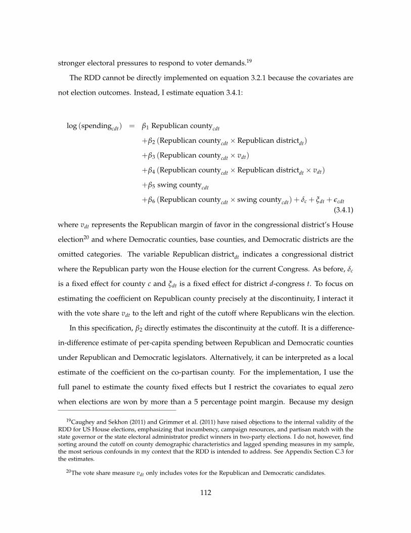
stronger electoral pressures to respond to voter demands.19

The RDD cannot be directly implemented on equation 3.2.1 because the covariates are

not election outcomes. Instead, I estimate equation 3.4.1:

log (spendingcdt) = β1 Republican countycdt

+β2 (Republican countycdt × Republican districtdt)

+β3 (Republican countycdt × vdt)

+β4 (Republican countycdt × Republican districtdt × vdt)

+β5 swing countycdt

+β6 (Republican countycdt × swing countycdt) + δc + ξdt + εcdt

(3.4.1)

where vdt represents the Republican margin of favor in the congressional district’s House

election20 and where Democratic counties, base counties, and Democratic districts are the

omitted categories. The variable Republican districtdt indicates a congressional district

where the Republican party won the House election for the current Congress. As before, δc

is a fixed effect for county c and ξdt is a fixed effect for district d-congress t. To focus on

estimating the coefficient on Republican county precisely at the discontinuity, I interact it

with the vote share vdt to the left and right of the cutoff where Republicans win the election.

In this specification, β2 directly estimates the discontinuity at the cutoff. It is a difference-

in-difference estimate of per-capita spending between Republican and Democratic counties

under Republican and Democratic legislators. Alternatively, it can be interpreted as a local

estimate of the coefficient on the co-partisan county. For the implementation, I use the

full panel to estimate the county fixed effects but I restrict the covariates to equal zero

when elections are won by more than a 5 percentage point margin. Because my design

19Caughey and Sekhon (2011) and Grimmer et al. (2011) have raised objections to the internal validity of theRDD for US House elections, emphasizing that incumbency, campaign resources, and partisan match with thestate governor or the state electoral administrator predict winners in two-party elections. I do not, however, findsorting around the cutoff on county demographic characteristics and lagged spending measures in my sample,the most serious confounds in my context that the RDD is intended to address. See Appendix Section C.3 forthe estimates.

20The vote share measure vdt only includes votes for the Republican and Democratic candidates.

112

includes district-congress fixed effects, the county covariates only pick-up the within-district

differences for the observations within the bandwidth. In Appendix Section C.3, I also

report estimates for bandwidths of 7.5 and 2.5 percentage points with similar results.21 In

all cases, I find null effects with the smallest standard errors under the largest bandwidth

and the largest standard errors under the smallest bandwidth.

Figure 3.3 illustrates the implementation of the RDD. For each percentile of the Republi-

can margin of favor in the House election, this graph plots the mean difference between

Republican and Democratic counties for all congressional districts where the vote share

is within that percentile. It also plots the linear polynomial from the RDD to the left and

right of the cutoff within the 5 percentage point bandwidth. The vertical difference at the

cutoff between these linear polynomials equals β2. The y-axis has been scaled to roughly

equal one within-district standard deviation of the spending measure. By this benchmark,

I find small point estimates at the discontinuity. Furthermore, the full panel beyond the

5 percentage point bandwidth exhibits limited differences between congressional districts

with small and large electoral margins in their within-district spending patterns.

Panel B of Table 3.2 reports the RDD estimates. Under the non-entitlement measure, I

find a point estimate of −0.0267 with a standard error of 0.0315 for the difference between

Republican and Democratic counties at the discontinuity. While not as precise as the

results from the full panel, it can still rule out increases in the difference in per-capita

spending between Republican and Democratic counties greater than 3.5 percentage points

when a congressional district switches from Democratic to Republican control under a 95

percent confidence interval. The other specifications also find insignificant results with

negative point estimates, although the discretionary and contracts measures have larger

upper bounds.

21Appendix Section C.3 compares RDD estimates using margins of 7.5, 5, and 2.5 percentage points.

113

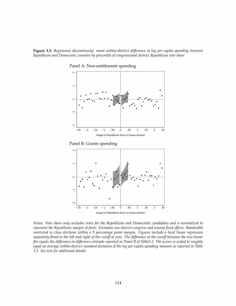
Figure 3.3: Regression discontinuity: mean within-district difference in log per-capita spending betweenRepublican and Democratic counties by percentile of congressional district Republican vote share

Panel A: Non-entitlement spending

−.2

−.1

0.1

.2

−.25 −.2 −.15 −.1 −.05 0 .05 .1 .15 .2 .25

margin of Republican favor in House election

Panel B: Grants spending

−.2

−.1

0.1

.2

−.25 −.2 −.15 −.1 −.05 0 .05 .1 .15 .2 .25

margin of Republican favor in House election

Notes: Vote share only includes votes for the Republican and Democratic candidates and is normalized torepresent the Republican margin of favor. Estimates use district-congress and county fixed effects. Bandwidthrestricted to close elections within a 5 percentage point margin. Figures include a local linear regressionseparately fitted to the left and right of the cutoff at zero. The difference at the cutoff between the two linearfits equals the difference-in-difference estimate reported in Panel B of Table3.2. The y-axis is scaled to roughlyequal an average within-district standard deviation of the log per-capita spending measure as reported in Table3.1. See text for additional details.

114

3.4.3 First-differences design

To isolate the identification from redistricting, I implement a first-differences version of

equation 3.2.1. By limiting the sample to only periods before and after redistricting where

the party of the House representative also remains unchanged, I focus on the immediate

changes in the within-district distribution of spending that follow redistricting. A potential

confound to this approach is that redistricting sometimes occurs in response to gradual

demographic changes, such as to balance population shifts or to protect minority districts.22

The distribution of federal spending may also respond to these demographic changes

because some federal formulas use US Census demographic estimates to determine their

geographic allocation. My design partially accounts for this issue by focusing on the

immediate within-district change and by using a per-capita spending measure based on the

annual US Census population estimates.

Equation 3.4.2 implements the first-differences design:

∆ log (spendingcdt) = β1 ∆ (co-partisan countycdt) + β2 ∆ (swing countycdt)

+β3 ∆ (co-partisan countycdt × swing countycdt) + ∆ξdt + ∆εcdt

(3.4.2)

where, as before, ξdt is a fixed effect for district d-congress t. Here, I have omitted the fixed

effect δc for county c because first-differences eliminates time-invariant variables.

Figure 3.4 displays estimates of the coefficient for the swing county. I also include lead

and lag estimates of this indicator as placebo tests for redistricting and as checks for pre-

and post-trends.23 The y-axis has been scaled to roughly equal one within-district standard

deviation of the spending measure. By this benchmark, the first-difference specification

22Redistricting can be politically motivated as well, particularly to protect friendly incumbents or to unseatopposing ones. Redistricting that creates a safer district could result in less targeting because legislators feel lesspressure to respond to voter demands. Conversely, redistricting that results in a more competitive district couldresult in more targeting because legislators feel more electoral pressure. On net, it is unclear whether this bias ispositive or negative, although Figure 3.3 for the RDD suggests that congressional districts with small and largeelectoral margins have similar within-district spending patterns.

23In Figure 3.4, the sample is only restricted to periods where the party remains unchanged in order toestimate the leads and lags in addition to the redistricting treatment. Because party switches are excluded,identification still solely comes from redistricting.

115

estimates a reasonably precise zero effect. The leads and lags do not suggest an obvious pre-

or post-trend that could be attributed to demographic changes. In addition, the standard

errors on the estimates are similar across treatment, leads, and lags.

Panel C of Table 3.2 reports estimates of equation 3.4.2. Under the non-entitlement

spending measure, I find an estimate of −0.0015 with a standard error of 0.0171 for the

swing county. This estimate rules out differences in per-capita spending with the base

opposition counties greater than 3.3 percentage points under a 95 percent confidence interval.

The results for the other spending measures and the co-partisan county are also not strongly

significant.

3.5 Robustness

The null effects found in the previous section could be criticized for largely excluding

urban counties. Because they receive greater overall levels of spending, legislators represent-

ing urban areas may have more opportunities to influence its within-district distribution.

Furthermore, my main results ignore variation in institutional context that may affect the

capacity of legislators to manipulate federal spending. In response, I provide estimates of

the within-state distribution of spending for the US Senate, where I can include all counties,

and I replicate my full panel estimates to account for (i) partisan alignment with the House

majority and the president, (ii) congressional committee assignments, and (iii) the bicameral

nesting of House and Senate districts in the US Congress. These considerations do not

substantively change my previous findings.

3.5.1 US Senate

Replicating my analysis using the US Senate allows me to include nearly all counties because

senators represent entire states.24 I report county sample summary statistics de-meaned

24This sample still excludes counties that contain a state capital because a significant amount of federalspending is mechanically allocated to them for accounting purposes, and then ultimately redistributed acrossthe state.

116

Figure 3.4: First-differences: lead and lag estimates of changes in log per-capita spending for swing counties

Panel A: Non-entitlement spending−

.2−

.10

.1.2

−3 −2 −1 0 1 2 3Congress relative to redistricting

Panel B: Grants spending

−.2

−.1

0.1

.2

−3 −2 −1 0 1 2 3Congress relative to redistricting

Notes: Error bars indicate a 95 percent confidence interval. Plotted estimates from equation 3.4.2, includingthree leads and lags. The sample is restricted to periods where the party of the House representative alsoremains unchanged. The y-axis is scaled to roughly equal an average within-district standard deviation of thelog per-capita spending measure as reported in Table 3.1. See text for additional details.

117

by state-congress and estimates that use the full panel and that include state-congress

and county fixed effects. Here, only counties under Democratic and Republican Senate

delegations are defined as either co-partisan or opposition.25 Furthermore, I exclude swing

counties from the analysis when including county fixed effects because all Senate delegations

share the same swing voters and states do not change their boundaries.

With these considerations, I estimate equation 3.5.1:

log (spendingcst) = β co-partisan countycst + δc + ξst + εcst (3.5.1)

where opposition county is the omitted category, δc is a fixed effect for county c, and ξst is a

fixed effect for state s-congress t. Here, β captures the mean within state-congress difference

between co-partisan and opposition counties.

Panel A of Table 3.3 reports partisan county quantile means for the spending measures.

All variables are de-meaned by state-congress. I do not report means for the bi-partisan

county quantiles because the two-candidate distributive politics models do not make clear

predictions for these cases. Similar to the patterns within congressional districts, swing

counties receive less spending than base opposition counties under all spending measures.

Furthermore, the differences between quantile means are a small fraction of the mean within

state-congress standard deviations. As before, the three models reviewed earlier do not

predict the observed patterns across partisan county quantile means.

Panel B of Table 3.3 reports estimates of equation 3.5.1. Under the non-entitlement

spending measure, I find a point estimate of −0.0080 with a standard error of 0.0093. Using

a 95 percent confidence internal, I can rule out differences between the co-partisan county

and the opposition county greater than 1.0 percentage points. I find similarly precise null

effects for the other spending measures. Including a broader sample of counties under the

US Senate delivers similar results as in the previous section for whether co-partisan counties

receive disproportionately more spending.

25I define counties under bi-partisan Senate delegations as bi-partisan. I cannot identify an effect on thisvariable because there is no within state-congress variation.

118

Table 3.3: US Senate: relative log per-capita spending across counties within states

log (per-capita federal spending)total non-entitlement discretionary grants contracts

Panel A: Summary statistics demeaned by state-congressbase co-partisan counties 0.0204 0.0732 0.0852 0.0318 0.1381

(0.3751) (0.5919) (0.6535) (0.5508) (1.3420)swing co-partisan counties -0.0139 -0.0457 -0.0687 -0.0873 -0.1485

(0.3429) (0.5549) (0.5995) (0.4850) (1.2448)swing opposition counties -0.0104 -0.0449 -0.0633 -0.0395 -0.1720

(0.3504) (0.5509) (0.5528) (0.4930) (1.2269)base opposition counties 0.0078 0.0339 0.0568 0.0636 0.1807

(0.3648) (0.5766) (0.6068) (0.5284) (1.3588)mean within district- 0.3501 0.5681 0.6060 0.4842 1.2900congress std. dev. (0.1172) (0.1581) (0.1790) (0.1357) (0.2727)

Panel B: Full panelco-partisan county -0.0121 -0.0080 0.0087 0.0107 -0.0371

(0.0079) (0.0093) (0.0132) (0.0151) (0.0263)county FE X X X X Xstate-congress FE X X X X Xno. of county-congresses 36,640 36,640 22,069 36,640 36,640no. of state-congresses 585 585 352 585 585no. of states 48 48 48 48 48

Notes: Standard errors in parentheses and clustered by state. Panel A does not report county quantile meansfor bi-partisan counties. Panel B estimates equation 3.5.1 where opposition county is the omitted category.Bi-partisan counties are not identified because the specification includes state-congress fixed effects. Withineach state-congress, counties are equally sorted into Republican and Democratic halves by their panel meanRepublican vote share in presidential elections. Under state senate delegations with either two Republicans ortwo Democrats, I define counties as co-partisan when their partisanship matches their state’s senate delegationand as opposition otherwise. Under bi-partisan senate delegations, I define all counties as bi-partisan. See textfor additional details. * - p-value < 0.10, ** - p-value < 0.05, *** - p-value < 0.01

119

3.5.2 Partisan alignment

Next, I replicate estimates for equation 3.2.1 with interactions for whether the House repre-

sentative shares the same party as the House majority and as the president. Identification

comes from the partisan switches in the House majority and the president in the time-series.

As before, I find null results with similar precision.

Table 3.4 reports the estimates. Under the non-entitlement measure for the interaction

with the House majority, I estimate a coefficient of 0.0065 with a standard error of 0.0125

for the co-partisan county and a coefficient of 0.0156 with a standard error of 0.0103 for

the swing county. These estimates allow me to rule out differences with base opposition

counties greater than 3.1 and 3.6 percentage points respectively using a 95 percent confidence

interval. For the interactions with the president’s party, I find a point estimate of 0.0163

with a standard error of 0.0119 on the co-partisan county and a point estimate of 0.0004 with

a standard error of 0.0133 on the swing county. Similarly, I can rule out differences with

base opposition counties greater than 3.9 and 2.7 percentage points respectively. Estimates

are also generally insignificant and precise for the grants spending measure. Although one

coefficient is marginally significant on the interaction between the swing county and the

House majority party, the p-values are not adjusted for multiple hypothesis tests. These

results do not suggest that the within-district allocations under House representatives

substantially differ under the partisan alignments tested here.

3.5.3 Congressional committees

I also consider interactions for committee chairs, ranking minority members, membership on

the Appropriations Committee, and membership on the Ways & Means Committee. Chairs

and ranking minority members are the most senior members of the committee from the

majority and minority parties respectively. The Appropriations Committee drafts the annual

appropriations bills for discretionary spending. The Ways & Means Committee writes

major tax legislation. These positions are generally considered influential and desirable

among House members. They serve as proxies to identify legislators with greater ability to

120

Table 3.4: Partisan alignment: relative log per-capita spending estimates using the full panel

log(per-capita federal spending)non-entitlement grants non-entitlement grants

co-partisan county -0.0104 -0.0025 -0.0142 0.0001(0.0113) (0.0133) (0.0109) (0.0112)

×House majority party 0.0065 0.0179(0.0125) (0.0126)

×president’s party 0.0163 0.0188(0.0119) (0.0140)

swing county -0.0093 -0.0237* 0.0004 -0.0166(0.0193) (0.0133) (0.0145) (0.0157)

×House majority party 0.0156 0.0226*(0.0103) (0.0121)

×president’s party 0.0004 0.0132(0.0133) (0.0118)

co-partisan county×swing county 0.0230 0.0083 0.0015 0.0031(0.0165) (0.0167) (0.0140) (0.0155)

×House majority party -0.0238 -0.0148(0.0174) (0.0201)

×president’s party 0.0127 -0.0087(0.0201) (0.0156)

county FE X X X Xdistrict-congress FE X X X Xno. of county-congresses 28,524 28,524 28,524 28,524no. of district-congresses 2,208 2,208 2,208 2,208no. of states 47 47 47 47

Notes: Standard errors in parentheses and clustered by state. Estimates equation 3.2.1, with added interactionsfor when the House representative shares the same party as the House majority and the president. Within eachdistrict-congress and using the Republican vote share in presidential elections, counties are equally sorted intoeither Republican or Democratic halves by their panel average and into either swing or base halves by theirpanel standard deviation. Counties are defined as co-partisan when their partisanship matches their Houserepresentative in the current Congress and are defined as opposition otherwise. See text for additional details. *- p-value < 0.10, ** - p-value < 0.05, *** - p-value < 0.01

121

influence federal spending.

Table 3.5 reports estimates for the committee interactions. Under the non-entitlement

measure, I estimate large and significantly negative coefficients when considering committee

chairs and ranking minority members. Among the committee chair interactions, I find a

point estimate of −0.0652 with a standard error of 0.0323 for the co-partisan county and

a point estimate of −0.0304 with a standard error of 0.0284 for the swing county. Using a

95 percent confidence interval, these estimates allow me to rule out differences with base

opposition counties greater than −0.2 percentage points and 2.5 percentage points. For the

ranking minority member interaction, I estimate a coefficient of −0.0770 with a standard

error of 0.0385 on the co-partisan county and a coefficient of −0.0708 with a standard error

of 0.0267 on the swing county. Similarly, I can rule out differences with base opposition

counties greater than −0.1 and −1.9 percentage points respectively. I neither, however,

replicate these results for the grants measure nor for the other committee interactions. In

these cases, I instead estimate reasonably precise zero effects as before.

The significant negative coefficients that I find are hard to interpret under the two-

candidate distributive politics models. Because I still estimate precise zeroes for the main

effects of the co-partisan and swing counties, these negative interactions imply that opposi-

tion counties receive the most spending under committee chairs and that base opposition

counties receive the most spending under ranking minority members. The models that I

test do not predict that the most influential legislators would target opposition voters with

spending.

3.5.4 Bicameralism

Finally, I account for the bicameral nesting of House districts within Senate districts in

the US Congress. Although a district-congress fixed effect will pick-up a common effect

from the state’s Senate delegation, senators may also be engaged in differential targeting

across counties. This interaction could matter if (i) House and Senate members substitute

between each other’s spending or (ii) House and Senate members cooperate to direct

122

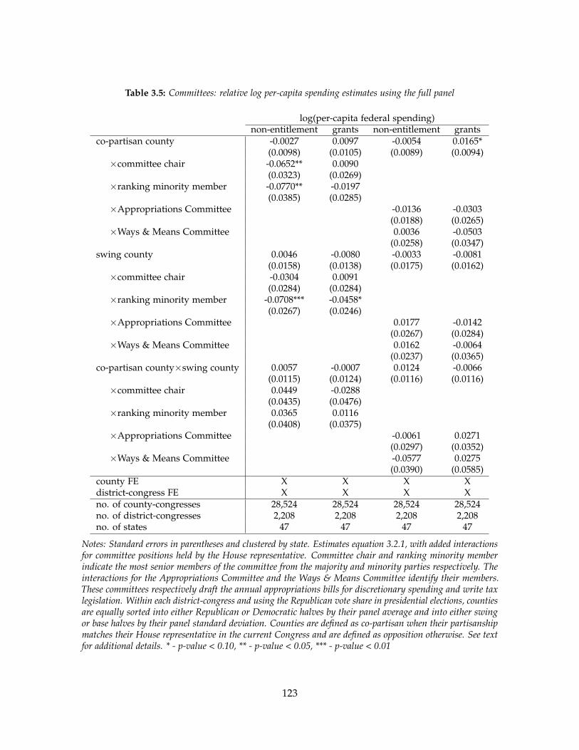
Table 3.5: Committees: relative log per-capita spending estimates using the full panel

log(per-capita federal spending)non-entitlement grants non-entitlement grants

co-partisan county -0.0027 0.0097 -0.0054 0.0165*(0.0098) (0.0105) (0.0089) (0.0094)

×committee chair -0.0652** 0.0090(0.0323) (0.0269)

×ranking minority member -0.0770** -0.0197(0.0385) (0.0285)

×Appropriations Committee -0.0136 -0.0303(0.0188) (0.0265)

×Ways & Means Committee 0.0036 -0.0503(0.0258) (0.0347)

swing county 0.0046 -0.0080 -0.0033 -0.0081(0.0158) (0.0138) (0.0175) (0.0162)

×committee chair -0.0304 0.0091(0.0284) (0.0284)

×ranking minority member -0.0708*** -0.0458*(0.0267) (0.0246)

×Appropriations Committee 0.0177 -0.0142(0.0267) (0.0284)

×Ways & Means Committee 0.0162 -0.0064(0.0237) (0.0365)

co-partisan county×swing county 0.0057 -0.0007 0.0124 -0.0066(0.0115) (0.0124) (0.0116) (0.0116)

×committee chair 0.0449 -0.0288(0.0435) (0.0476)

×ranking minority member 0.0365 0.0116(0.0408) (0.0375)

×Appropriations Committee -0.0061 0.0271(0.0297) (0.0352)

×Ways & Means Committee -0.0577 0.0275(0.0390) (0.0585)

county FE X X X Xdistrict-congress FE X X X Xno. of county-congresses 28,524 28,524 28,524 28,524no. of district-congresses 2,208 2,208 2,208 2,208no. of states 47 47 47 47

Notes: Standard errors in parentheses and clustered by state. Estimates equation 3.2.1, with added interactionsfor committee positions held by the House representative. Committee chair and ranking minority memberindicate the most senior members of the committee from the majority and minority parties respectively. Theinteractions for the Appropriations Committee and the Ways & Means Committee identify their members.These committees respectively draft the annual appropriations bills for discretionary spending and write taxlegislation. Within each district-congress and using the Republican vote share in presidential elections, countiesare equally sorted into either Republican or Democratic halves by their panel average and into either swingor base halves by their panel standard deviation. Counties are defined as co-partisan when their partisanshipmatches their House representative in the current Congress and are defined as opposition otherwise. See textfor additional details. * - p-value < 0.10, ** - p-value < 0.05, *** - p-value < 0.01

123

spending to geographic areas they both favor. For the same rationales expressed in Section

3.5.1, I only consider Senate co-partisan counties under Democratic and Republican Senate

delegations. In estimation, I include main effects for House co-partisan, House swing, and

Senate co-partisan counties, their interactions, and district-congress and county fixed effects.

Table 3.6 reports the results accounting for bicameralism. The estimates are generally

insignificant and precise as before. For the main effects on the House co-partisan and swing

counties under the non-entitlement measure, I find point estimates of 0.0009 and 0.0117

with standard errors of 0.0099 and 0.0180 respectively. The upper bounds of a 95 percent

confidence interval allow me rule out differences with base opposition counties greater than

2.0 and 4.7 percentage points. For their interactions with the Senate co-partisan county, I

report point estimates of −0.0263 and −0.0401 with standard errors of 0.0203 and 0.0216

respectively. I can rule out differences with base opposition counties greater than 1.3 and

0.2 percentage points. Although the negative interactions suggest substitution, they are not

strongly significant. Furthermore, I estimate reasonably precise zeroes for the main effects.

Accounting for nested districts in the bicameral legislature has little impact on my initial

results.

3.6 Conclusion

This paper finds that neither the co-partisan nor swing counties within a sub-sample of

congressional districts receive substantially more federal spending when broad measures

are considered in a 1982-2006 panel of US House elections. I find similar results when I

implement a RDD on two-party elections and a first-differences design on redistricting.

Furthermore, I estimate reasonably precise null effects when I consider the US Senate,

partisan alignment, congressional committees, and the nested districts of the bicameral

US Congress. Standard distributive politics models do not predict the flat distribution

of spending that I find across geographic clusters of voters. At least three alternative

explanations emerges from previous research.

First, checks and balances within the federal budget process may prevent legislators from

124

Table 3.6: Bicameralism: relative log per-capita spending estimates using the full panel

log (per-capita federal spending)total non-entitlement discretionary grants contracts

House co-partisan county -0.0008 0.0009 0.0134 0.0130 0.0084(0.0063) (0.0099) (0.0150) (0.0109) (0.0239)

House swing county 0.0123 0.0117 -0.0009 -0.0030 -0.0584(0.0098) (0.0180) (0.0275) (0.0150) (0.0468)

House co-partisan county× -0.0003 -0.0006 -0.0178 -0.0053 0.0368House swing county (0.0062) (0.0104) (0.0167) (0.0112) (0.0374)

Senate co-partisan county 0.0076 0.0279 0.0365 0.0167 0.0384(0.0108) (0.0176) (0.0282) (0.0187) (0.0407)

House co-partisan county× -0.0148 -0.0263 -0.0178 -0.0138 -0.0821Senate co-partisan county (0.0109) (0.0203) (0.0312) (0.0225) (0.0608)

House swing county× -0.0189* -0.0401* -0.0371 -0.0246 -0.0360Senate co-partisan county (0.0111) (0.0216) (0.0316) (0.0188) (0.0540)

House co-partisan×House 0.0173 0.0308 0.0086 0.0155 0.0645swing×Senate co-partisan (0.0143) (0.0233) (0.0335) (0.0292) (0.0877)

county FE X X X X Xdistrict-congress FE X X X X Xno. of county-congresses 28,524 28,524 17,815 28,524 28,524no. of district-congresses 2,208 2,208 1,355 2,208 2,208no. of states 47 47 47 47 47

Notes: Standard errors in parentheses and clustered by state. Estimates equation 3.2.1, with a main effectand interactions added for the Senate co-partisan counties. House co-partisan and swing counties are definedrelative to other counties within each district-congress and depend on the partisan match with their Houserepresentative. Senate co-partisan counties are defined relative to other counties within each state-congressand depend on the partisan match with their state’s Senate delegation. Both use the Republican vote share inpresidential elections to sort counties into Republican and Democratic halves by their panel mean and intoswing and base halves by the panel standard deviation. Counties are defined as co-partisan when they matchthe partisanship of their legislator(s) and conversely for opposition counties. See text for additional details. * -p-value < 0.10, ** - p-value < 0.05, *** - p-value < 0.01

125

steering resources toward co-partisan and swing voters. The welfare costs from allowing

legislators to manipulate federal spending for electoral purposes may be so large that

legislators prefer to commit themselves to impartial budgetary rules. A large literature

(Alesina and Perotti 1996, Alt and Lowry 1994, Besley and Case 2003, Ferejohn and Krehbiel

1987, Poterba 1996) has explored the effects of alternative budgetary institutions on fiscal

policy outcomes. Although I partially account for this issue by accounting for partisan

alignment, congressional committees, and bicameralism to identify legislators with greater

capacity to influence federal spending, there could still be particulars about the rules

regulating the budget process that prevent spending aggregates from benefiting one group

of voters over another.

Second, the direct personal impact of candidate policy positions may not determine

whom voters choose to support. Meehl (1977)argues it unlikely that voters choose between

candidates on the basis of personal material benefit because any individual voter has a negli-

gible probability of being pivotal in an election. Rather, social altruism may provide a more

plausible basis for voting behavior. Under this assumption, ideologically heterogeneous

tastes can still play a role among voters in their preferred programmatic composition of

government spending

Third, imperfect information among voters about public policy may break the predictions

from the two-candidate distributive politics models (Lupia 1992). If voters are largely

ignorant about federal spending, then they can neither reward nor punish politicians for

manipulating its distribution. Legislators may instead expend their effort on securing federal

benefits for well-informed special interests at the expense of the general public (Lohmann

1998).

While this paper finds evidence that the victors do indeed share the spoils, future

research is needed to understand why. My empirical results cannot distinguish between the

three alternative interpretations discussed here. Previous positive results for the relevance

of politics in the distribution of federal spending suggest against the checks and balances

interpretation. For the distributive politics literature in particular, a flat distribution of

126

federal spending aggregates could mask either partisan differences in the programmatic

composition of spending, narrow targeting of spending to interest groups, or an emphasis

on highly salient government spending projects for political campaigning.

127

References

Abel, Andrew B. 1982. “Dynamic Effects of Permanent and Temporary Tax Policies in a qModel of Investment.” Journal of Monetary Economics, 9: 353–373.

Abel, Andrew B. 1990. “Consumption and Investment.” Handbook of Monetary Economics.

Abel, Andrew B., and Janice C. Eberly. 1994. “A Unified Model of Investment UnderUncertainty.” American Economic Review, 1369–1384.

Aizer, Anna. 2007. “Public Health Insurance, Program Take-up, and Child Health.” Reviewof Economics and Statistics, 89(3): 400–415.

Akerlof, George A. 1991. “Procrastination and obedience.” American Economic Review,81(2): 1–19.

Albouy, David. 2013. “Partisan Representation in Congress and the Geographic Distributionof Federal Funds.” Review of Economics and Statistics, 95(1): 127–141.

Alesina, Alberto, and Roberto Perotti. 1996. “Fiscal Discipline and the Budget Process.”American Economic Review Papers and Proceedings, 86(2): 401–407.

Almeida, Heitor, Murillo Campello, and Michael S. Weisbach. 2004. “The Cash FlowSensitivity of Cash.” Journal of Finance, 59(4): 1777–1804.

Alt, James E., and Robert C. Lowry. 1994. “Divided Government, Fiscal Institutions andBudget Deficits: Evidence from the States.” American Political Science Review, 88(4): 811–828.

Altshuler, Rosanne, Alan Auerbach, Michael Cooper, and Matthew Knittel. 2009. “Un-derstanding U.S. Corporate Tax Losses.” Tax Policy and the Economy, 23: 73–122.

Altshuler, Rosanne, and Alan J. Auerbach. 1990. “The Significance of Tax Law Asymme-tries: An Empirical Investigation.” Quarterly Journal of Economics, 105(1): 61–86.

Alvarez, R. Michael, and Jason L. Lowry. 1997. “Congressional Committees and the Politi-cal Economy of Federal Outlays.” Public Choice, 92(1-2): 55–73.

Ansolabehere, Stephen, and James M. Snyder, Jr. 2006. “Party Control of State Governmentand the Distribution of Public Expenditures.” The Scandanavian Journal of Economics,108(4): 547–569.

Armstrong, Chris, Jennifer L. Blouin, and David F. Larcker. 2012. “The Incentives for TaxPlanning.” Journal of Accounting and Economics, 53(1-2): 391–411.

128

Auerbach, Alan J., and James M. Poterba. 1987a. “Tax-Loss Carryforwards and CorporateTax Incentives.” In The Effects of Taxation on Capital Accumulation. Vol. I, 305–342.

Auerbach, Alan J., and James M. Poterba. 1987b. “Tax loss carryforwards and corporate taxincentives.” In The effects of taxation on capital accumulation. 305–342. University of ChicagoPress.

Auerbach, Alan J., and Kevin A. Hassett. 1992. “Tax policy and business fixed investmentin the United States.” Journal of Public Economics, 47(2): 141–170.

Balla, Steven J., Eric D. Lawrence, Forrest Maltzman, and Lee Sigelman. 2002. “Partisan-ship, Blame Avoidance, and the Distribution of Legislative Pork.” American Journal ofPolitical Science, 46(3): 515–525.

Baron, David P., and John A. Ferejohn. 1989. “Bargaining in Legislatures.” American PoliticalScience Review, 83(4): 1181–1206.

Berry, Christopher R., Barry C. Burden, and William G. Howell. 2010. “The President andthe Distribution of Federal Spending.” American Political Science Review, 104(4): 783–799.

Bertrand, Marianne, and Antoinette Schoar. 2003. “Managing with Style: The Effect ofManagers on Firm Policies.” Quarterly Journal of Economics, 118(4): 1169–1208.

Bertrand, Marianne, Esther Duflo, and Sendhil Mullainathan. 2004. “How Much ShouldWe Trust Differences-In-Differences Estimates?” Quarterly Journal of Economics, 119(1): 249–275.

Besley, Timothy, and Anne Case. 2003. “Political Institutions and Policy Choices: Evidencefrom the United States.” Journal of Economic Literature, 41(1): 7–73.

Bickers, Kenneth N., and Robert M. Stein. 2000. “The Congressional Pork Barrel in aRepublican Era.” Journal of Politics, 62(4): 1070–1086.

Bitler, Marianne P., Janet Currie, and John Karl Scholz. 2003. “WIC Eligibility and Partici-pation.” Journal of Human Resources, 38: 1139–1179.

Bloom, Nicholas, and John Van Reenen. 2007. “Measuring and Explaining ManagementPractices Across Firms and Countries.” Quarterly Journal of Economics, 122(4): 1351–1408.

Bloom, Nicholas, Benn Eifert, Aprajit Mahajan, David McKenzie, and John Roberts.2013. “Does Management Matter? Evidence from India.” Quarterly Journal of Economics,128(1): 1–51.

Bond, Stephen, and John Van Reenen. 2007. “Microeconometric Models of Investment andEmployment.” In Handbook of Econometrics. Vol. 6, Chapter 65, 4417–4498.

Bureau, US Census. 2010. Consolidated Federal Funds Report. Washington, DC:US CensusBureau.

Caballero, Ricardo J., and Eduardo MRA Engel. 1999. “Explaining investment dynamicsin US manufacturing: a generalized (S, s) approach.” Econometrica, 67(4): 783–826.

129

Carsey, Thomas M., and Barry Rundquist. 1999. “Party and Committee in DistributivePolitics: Evidence from Defense Spending.” Journal of Politics, 61(4): 1156–1169.

Caughey, Devin, and Jasjeet S. Sekhon. 2011. “Elections and the Regression DiscontinuityDesign: Lessons from Close U.S. House Races, 1942–2008.” Political Analysis, 19(4): 385–481.

Chaney, Thomas, David Sraer, and David Thesmar. 2012. “The Collateral Channel: HowReal Estate Shocks affect Corporate Investment.” American Economic Review, 102(6): 2381–2409.

Chetty, Raj. 2012. “Bounds on Elasticities with Optimization Frictions: A Synthesis of Microand Macro Ecidence on Labor Supply.” Econometrica, 80(3): 969–1018.

Chetty, Raj, Adam Looney, and Kory Kroft. 2009. “Salience and Taxation: Theory andEvidence.” American Economic Review, 99(4): 1145–1177.

Chetty, Raj, and Emmanuel Saez. 2013. “Teaching the Tax Code: Earnings Responses toan Experiment with EITC Recipients.” American Economic Journal: Applied Economics,5(1): 1–31.

Chetty, Raj, John Friedman, and Emmanuel Saez. 2013. “Using Differences in KnowledgeAcross Neighborhoods to Uncover the Impacts of the EITC on Earnings.” AmericanEconomic Review, 103(7): 2683–2721.

Chetty, Raj, John N. Friedman, Tore Olsen, and Luigi Pistaferri. 2011. “Adjustment Costs,Firm Responses, and Micro vs. Macro Labor Supply Elasticities: Evidence from DanishTax Records.” Quarterly Journal of Economics, 126(2): 749–804.

Chirinko, Robert S., Steven M. Fazzari, and Andrew P. Meyer. 1999. “How responsive isbusiness capital formation to its user cost? An exploration with micro data.” Journal ofPublic Economics, 74: 53–80.

Cohen, Darrel, Dorthe-Pernille Hansen, and Kevin A. Hassett. 2002. “The effects of tem-porary partial expensing on investment incentives in the United States.” National TaxJournal, 55(3).

Committee on Ways & Means. 2003. “Report 108-94: Jobs and Growth Reconciliation TaxAct of 2003.” U.S. House of Representatives.

Cooper, Russell, and John Haltiwanger. 2006. “On the Nature of Capital Adjustment Costs.”Review of Economic Studies, 73(3): 611–633.

Cummins, Jason G., Kevin A. Hassett, and R. Glenn Hubbard. 1994. “A Reconsiderationof Investment Behavior Using Tax Reforms as Natural Experiments.” Brookings Papers onEconomic Activity, 2: 1–74.

Cummins, Jason G., Kevin A. Hassett, and R. Glenn Hubbard. 1995. “Have tax reformsaffected investment?” In Tax Policy and the Economy, Volume 9. 131–150. MIT Press.

130

Cummins, Jason G., Kevin A. Hassett, and R. Glenn Hubbard. 1996. “Tax Reforms andInvestment: A Cross-Country Comparison.” Journal of Public Economics, 62(1-2): 237–273.

Currie, Janet. 2006. “The Take Up of Social Benefits.” In Public Policy and the Income Distribu-tion. , ed. Alan J. Auerbach, David Card and John M. Quigley. New York, NY:Russell SageFoundation Publications.

Currie, Janet, and Jeffrey Grogger. 2001. “Explaining Recent Declines in Food StampProgram Participation.” Brookings-Wharton Papers on Urban Affairs, 203–244.

Daponte, Beth Osborne, Sanders Seth, and Lowell Taylor. 1999. “Why Do Low-IncomeHouseholds not Use Food Stamps? Evidence from an Experiment.” Journal of HumanResources, 34(3): 612–628.

Desai, Mihir A., and Austan D. Goolsbee. 2004. “Investment, overhang, and tax policy.”Brookings Papers on Economic Activity, 35(2): 285–355.

Dew-Becker, Ian. 2012. “Investment and the Cost of Capital in the Cross-Section: The TermSpread Predicts the Duration of Investment.” mimeo.

Dixit, Avinash, and John Londregan. 1996. “The Determinants of Success of Special Inter-ests in Redistributive Politics.” Journal of Politics, 58(4): 1132–1155.

Dyreng, Scott D., Michelle Hanlon, and Edward L. Maydew. 2010. “The Effects of Execu-tives on Corporate Tax Avoidance.” The Accounting Review, 85(4): 1163–1189.

Edgerton, Jesse. 2010. “Investment incentives and corporate tax asymmetries.” Journal ofPublic Economics, 94(11-12): 936–952.

Farre-Mensa, Joan, and Alexander Ljungqvist. 2013. “Do Measures of Financial ConstraintsMeasure Financial Constraints?” NBER Working Paper No. 19551.

Faulkender, Michael, and Rong Wang. 2006. “Corporate financial policy and the value ofcash.” Journal of Finance, 61(4): 1957–1990.

Fazzari, Steven M., R. Glenn Hubbard, and Bruce C. Petersen. 1988a. “Financing Con-straints and Corporate Investment.” Brookings Papers on Economic Activity, 1988(1): 141–195.

Fazzari, Steven M., R. Glenn Hubbard, and Bruce C. Petersen. 1988b. “Investment, Fi-nancing Decisions, and Tax Policy.” American Economic Review: Papers and Proceedings,78(2): 200–205.

Ferejohn, John A. 1974. Pork Barrel Politics: Rivers and Harbors Legislation, 1947-1968. Stanford,CA:Stanford University Press.

Ferejohn, John, and Keith Krehbiel. 1987. “The Budget Process and the Size of the Budget.”American Journal of Political Science, 31(2): 296–320.

Finkelstein, Amy. 2009. “EZ-Tax: Tax Salience and Tax Rates.” Quarterly Journal of Economics,124(3): 969–1010.

131

Goldin, Jacob, and Tatiana Homonoff. 2013. “Smoke Gets in Your Eyes: Cigarette TaxSalience and Regressivity.” American Economic Journal: Economic Policy, 5(1): 302–336.

Goolsbee, Austan. 1998. “Investment Tax Incentives, Prices, and the Supply of CapitalGoods.” Quarterly Journal of Economics, 113(1): 121–148.

Graham, John R. 1996. “Proxies for the corporate marginal tax rate.” Journal of FinancialEconomics, 42(2): 187–221.

Graham, John R. 2000. “How big are the tax benefits of debt?” Journal of Finance, 55(5): 1901–1941.

Graham, John R., and Lillian F. Mills. 2008. “Using tax return data to simulate corporatemarginal tax rates.” Journal of Accounting & Economics, 46(2-3): 366–388.

Grimmer, Justin, Eitan Hersh, Brian Feinstein, and Daniel Carpenter. 2011. “Are CloseElections Randomly Determined?” Working paper.

Hall, Robert E., and Dale W. Jorgenson. 1967. “Tax Policy and Investment Behavior.”American Economic Review, 57(3): 391–414.

Hassett, Kevin A., and R. Glenn Hubbard. 2002. “Tax Policy and Business Investment.”Handbook of Public Economics, 3.

Hausman, Jerry A. 1981. “Labor Supply.” In How Taxes Affect Economic Behavior. , ed. HenryAaron and Joseph Pechman, 27–71. Washington, D.C.:Brookings Institution Press.

Hayashi, Fumio. 1982. “Tobin’s Marginal q and Average q: A Neoclassical Interpretation.”Econometrica, 50(1): 213–224.

Heckman, James J., and Jeffrey A. Smith. 2004. “The Determinants of Participation in aSocial Program: Evidence from a Prototypical Job Training Prorgam.” Journal of LaborEconomics, 22(2): 243–298.

Heitshusen, Valerie. 2001. “The Allocation of Federal Money to House Committee Members:Distributive Theory and Policy Jurisdictions.” American Politics Research, 29(1): 79–97.

Hirano, Shigeo, James M. Snyder, Jr., and Michael M. Ting. 2009. “Distributive Politicswith Primaries.” Journal of Politics, 71(4): 1467–1480.

House, Christopher, and Matthew Shapiro. 2008. “Temporary Investment Tax Incentives:Theory with Evidence from Bonus Depreciation.” American Economic Review, 98(3): 737–68.

Internal Revenue Service. 2009. “Return Preparer Review.” Publication 4832 (Rev. 12-2009)Catalog Number 54419P.

Internal Revenue Service. 2014. “SOI Tax Stats: Integrated Business Data.”

Jackson, C. Kirabo, and Elias Bruegmann. 2009. “Teaching Students and Teaching EachOther: The Importance of Peer Learning for Teachers.” American Economic Journal: AppliedEconomics, 1(4): 85–108.

132

Kaplan, Steven N., and Luigi Zingales. 1997. “Do Investment-Cash Flow SensitivitiesProvide Useful Measures of Financing Constraints?” Quarterly Journal of Economics,112(1): 169–215.

Kaplan, Steven N., Mark M. Klebanov, and Morten Sorensen. 2012. “Which CEO Charac-teristics Matter?” Journal of Finance, 67(3): 973–1007.

Kitchen, John, and Matthew Knittel. 2011. “Business Use of Special Provisions for Accel-erated Deprecition: Section 179 Expensing and Bonus Deprecition, 2002-2009.” Workingpaper.

Klassen, Kenneth, Petro Lisowsky, and Devan Mescall. 2012. “Corporate tax compliance:The role of internal and external preparers.” Working paper.

Knight, Brian. 2005. “Estimating the Value of Proposal Power.” American Economic Review,95(5): 1639–1652.

Knittel, Matthew. 2007. “Corporate Response to Accelerated Tax Depreciation: BonusDepreciation For Tax Years 2002-04.” OTA Working Paper 98, 77(5): 1339–69.

Knittel, Matthew, Susan Nelson, Jason Debacker, John Kitchen, James Pearce, andRichard Prisinzano. 2011. “Methodology to Identify Small Businesses and Their Owners.”OTA Working Paper, , (August).

Koijen, Ralph SJ, and Motohiro Yogo. 2012. “The cost of financial frictions for life insurers.”NBER Working Paper No. 18321.

Laibson, David I. 1997. “Golden Eggs and Hyperbolic Discounting.” Quarterly Journal ofEconomics, 112(2): 443–477.

Laibson D. Repetto, A, and J Tobacman. 2007. “Estimating Discount Functions with Con-sumption Choices over the Lifecycle.” Economics Series Working Papers.

Lamont, Owen. 1997. “Cash Flow and Investment: Evidence from Internal Capital Markets.”Journal of Finance, 52(1): 83–109.

Larcinese, Valentino, James M. Snyder, Jr., and Cecilia Testa. 2013. “Testing Models ofDistributive Politics using Exit Polls to Measure Voters’ Preferences and Partisanship.”British Journal of Political Science, 43(4): 845–875.

Larcinese, Valentino, Leonzio Rizzo, and Cecilia Testa. 2006. “Allocating the U.S. FederalBudget to the States: The Impact of the President.” Journal of Politics, 68(2): 447–456.

Laslier, Jean-François, and Nathalie Picard. 2002. “Distributive Politics and Electoral Com-petition.” Journal of Economic Theory, 103(1): 106–130.

Lauderdale, Benjamin E. 2008. “Pass the Pork: Measuring Legislator Shares in Congress.”Political Analysis, 16(3): 235–249.

Lee, David S. 2008. “Randomized Experiments from Non-Random Selection in U.S. HouseElections.” Journal of Econometrics, 142(2): 675–697.

133

Lee, David S., and Thomas Lemieux. 2010. “Regression Discontinuity Designs in Eco-nomics.” Journal of Economic Literature, 48(2): 281–355.

Lee, Frances E. 2003. “Geographic Politics in the U.S. House of Representatives: CoalitionBuilding and Distribution of Benefits.” American Journal of Political Science, 47(4): 714–728.

Levitt, Steven D., and James M. Poterba. 1999. “Congressional Distributive Politics andState Economic Performance.” Public Choice, 99(1-2): 185–216.

Levitt, Steven D., and James M. Snyder, Jr. 1995. “Political Parties and the Distribution ofFederal Outlays.” American Journal of Political Science, 39(4): 958–980.

Lindbeck, Assar, and Jörgen W. Weibull. 1987. “Balanced-Budget Redistribution as theOutcome of Political Competition.” Public Choice, 52(3): 273–297.

Lohmann, Susanne. 1998. “An Information Rationale for the Power of Special Interests.”American Political Science Review, 92(4): 809–827.

Lupia, Arthur. 1992. “Busy Voters, Agenda Control, and the Power of Information.” AmericanPolitical Science Review, 86(2): 390–403.

Martin, Paul S. 2003. “Voting’s Rewards: Voter Turnout, Attentive Publics, and Congres-sional Allocation of Federal Money.” American Journal of Political Science, 47(1): 110–127.

McCarty, Nolan M. 2000. “Presidential Pork: Executive Veto Power and Distributive Politics.”American Political Science Review, 94(1): 117–129.

McKelvey, Richard D., and Raymond Riezman. 1992. “Seniority in Legislatures.” AmericanPolitical Science Review, 86(4): 951–965.

Meehl, Paul E. 1977. “The Selfish Voter Paradox and the Thrown-Away Vote Argument.”American Political Science Review, 71(1): 11–30.

Mills, Lillian, Kaye Newberry, and William Trautman. 2002. “Trends in Book-Tax Incomeand Balance Sheet Differences.” Tax Notes, 96(8).

Moffit, Robert A., ed. 2003. Means-Tested Transfer Programs in the United States. Universityof Chicago Press.

Myerson, Roger B. 1993. “Incentives to Cultivate Favored Minorities under AlternativeElectoral Systems.” American Political Science Review, 87(4): 856–869.

Poterba, James M. 1996. “Budget Institutions and Fiscal Policy in the U.S. States.” AmericanEconomic Review Papers and Proceedings, 86(2): 395–400.

Rauh, Joshua D. 2006. “Investment and financing constraints: Evidence from the fundingof corporate pension plans.” Journal of Finance, 61(1): 33–72.

Saez, Emmanuel. 2010. “Do Taxpayers Bunch at Kink Points?” American Economic Journal:Economic Policy, 2(3): 180–212.

134

Senate, US. 1995-2003. Appropriations, Budget Estimates, Etc. Washington, DC:US GovernmentPrinting Office.

Shepsle, Kenneth A., Robert P. Van Houweling, Samuel J. Abrams, and Peter C. Hanson.2009. “The Senate Electoral Cycle and Bicameral Appropriations Politics.” American Journalof Political Science, 53(2): 343–359.

Stein, Jeremy C. 1989. “Efficient capital markets, inefficient firms: A model of myopiccorporate behavior.” Quarterly Journal of Economics, 104(4): 655–669.

Stein, Jeremy C. 2003. “Agency, information and corporate investment.” Handbook of theEconomics of Finance, 1: 109–163.

Steuerle, Gene. 2008. “Some Ignored Costs of Bonus Depreciation.” Tax Notes.

Summers, Lawrence H. 1981. “Taxation and Corporate Investment: A q-Theory Approach.”Brookings Papers on Economic Activity, 1981(1): 67–140.

Summers, Lawrence H. 1987. “Investment incentives and the discounting of depreciationallowances.” In The effects of taxation on capital accumulation. 295–304. University of ChicagoPress.

The Recovery Accountability and Transparency Board. 2014. “Overview of Funding.”

Tobin, James. 1969. “A General Equilibrium Approach to Monetary Theory.” Journal ofMoney, Credit and Banking Credit and Banking, 1(1): 15–29.

US Department of Labor, Employment & Training Administration. 2014. “UnemploymentInsurance Data.”

Yagan, Danny. 2013. “Capital Tax Reform and the Real Economy: The Effects of the 2003Dividend Tax Cut.” mimeo.

Zwick, Eric, and James Mahon. 2014. “Do Financial Frictions Amplify Fiscal Policy? Evi-dence from Business Investment Stimulus.” Working paper.

135

Appendix A

Appendix to Chapter 1

A.1 Simulation of Tax Refunds for the Carryback Election

The IRS does not automatically compute the eligible carryback refund each time a corpora-

tion files an income tax return that reports a net operating loss. Instead, the IRS requires

firms to provide documentation that details the computation of their refund when they file

for it. To determine whether firms are eligible for carryback refunds, we simulate eligible

refunds based on each firm’s reported loss, their history of taxes paid in prior tax years, and

the policy rules detailed in Table 1.1. We validate the accuracy of our simulated refunds by

comparing them to claimed refunds.

Specifically, we identify each corporate tax return that reports a net operating loss. For

each firm, we pull their tax liability history and incorporate any post-filing adjustments to

their past tax returns. We then infer each firm’s past taxable income using their past tax

liabilities. This assumption ignores adjustments to tax liability from Schedule J of Form

1120, such as the application of tax credits and the alternative minimum tax. We next apply

the reported loss against our simulation of past taxable income according to the policy rules

in Table 1.1. We start by deducting the loss against the earliest eligible tax year and progress

in calendar order, until we have exhausted either the loss or all eligible taxable income. We

then re-compute the firm’s tax liability based on their new taxable income in each past tax

136

year. Finally, we calculate the carryback refund by taking the difference in the firm’s tax

liability before and after applying the carryback deduction.

We check the credibility of our simulation of eligible carryback refunds by comparing

them to the observed refunds received by firms that claim the carryback. Appendix Figure

A.1 plots means of log (claimed refunds) by vigintiles of log (simulated refunds). A uni-

variate regression of log (claimed refunds) on log (simulated refunds) yields a coefficient of

0.9636 and a R-squared of 0.9336. These results imply that we simulate the eligible carryback

refunds with a high degree of accuracy.

A.2 Simulation of Carryforward Deductions

We compute the net present values of the carryback and carryforward elections by simulating

future carryforward deductions. For each firm, we use the observed taxable income in future

tax periods. We first compute the amount of tax loss available for carryforward deductions.

For firms that elect the carryback, this amount equals the remaining amount of deductions

that could not be applied to past taxable income. For firms that elect the carryforward, this

amount equals the full loss reported at time t = 0.

We then simulate the claiming of the carryforward deduction against future taxable

income. We assume that firms deduct the carryforwards as soon as possible. Our simulation

can also account for firms that have an existing stock of carryforwards prior to time t = 0.

In these cases, we first deduct from the stock of pre-existing carryforwards before we deduct

the carryforwards generated by the tax loss at time t = 0. This treatment increases the

delayed realization of the tax benefits from the carryforwards.

A.3 Variable Definitions from the Business Tax Data

We pull line items from the income tax return, Form 1120, to describe characteristics of the

tax loss firms in our sample. Here, we explain how we construct the variables reported

in Table 1.2. All dollar amounts are normalized to 2013 price levels. Revenue equals total

137

income (line 11) plus cost of goods sold (line 2). Assets is reported in box D on the front

page of Form 1120. Payroll is the sum of W-2 and 1099-MISC wage statements. Firms issue

these statements to employees and contractors respectively. EBITDA is defined as total

income (line 11) minus total deductions (line 27) plus compensation of officers (line 12)

plus interest (line 19) plus charitable contributions (line 19) plus depreciation (line 20) plus

depletion (line 21) plus domestic production activities deduction (line 25).

We identify the paid preparer that assisted a corporation with filing their tax return

from Form 1120. On the bottom of the front page of the tax form, preparers hired to file an

income tax return must self-identify themselves and their employing firm. This field does

not include internal employees that prepare their employer’s income tax return.

We construct measures of preparers using the identifiers reported on Form 1120. We

match these identifiers to their individual income tax returns. We obtain our age variable

from a social security file that records the date of birth. We also compute average client

characteristics and the number of clients from the population of C and S corporations by

preparer and tax year. Similarly, we match tax firm identifiers to income tax returns for

sole-proprietorships, partnerships, and corporations to construct our measures for tax firms.

138

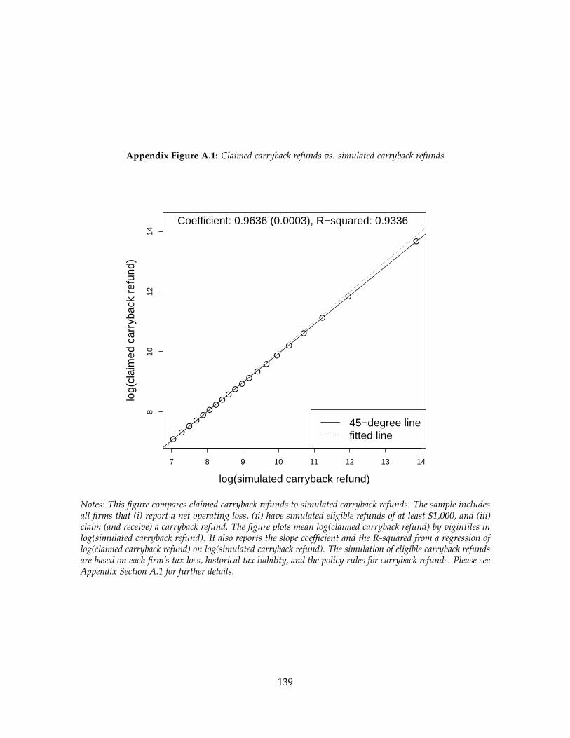
Appendix Figure A.1: Claimed carryback refunds vs. simulated carryback refunds

●●

●●

●●

●●

●●

●●

●●

●

●

●

●

●

●

7 8 9 10 11 12 13 14

810

1214

log(simulated carryback refund)

log(

clai

med

car

ryba

ck r

efun

d)

Coefficient: 0.9636 (0.0003), R−squared: 0.9336

45−degree linefitted line

Notes: This figure compares claimed carryback refunds to simulated carryback refunds. The sample includesall firms that (i) report a net operating loss, (ii) have simulated eligible refunds of at least $1,000, and (iii)claim (and receive) a carryback refund. The figure plots mean log(claimed carryback refund) by vigintiles inlog(simulated carryback refund). It also reports the slope coefficient and the R-squared from a regression oflog(claimed carryback refund) on log(simulated carryback refund). The simulation of eligible carryback refundsare based on each firm’s tax loss, historical tax liability, and the policy rules for carryback refunds. Please seeAppendix Section A.1 for further details.

139

Appendix B

Appendix to Chapter 2

B.1 Investment with Adjustment Costs and a Borrowing Constraint

We develop an infinite horizon, non-stochastic investment model, deriving the testable

hypotheses in Section 2.2 and the empirical moments for calibration in Section 2.5.3. The

model nests the standard neoclassical investment model with adjustment costs (Hayashi,

1982), a model with credit constraints and a model with managerial myopia.

B.1.1 General Setup

We begin with a discrete time version of Hayashi (1982). Firm value, V0, is given by an

infinite series of discounted net receipts, Rt. The discount rate, rt, is risk-adjusted and

possibly time varying. The expression for firm value is

V0 =∞

∑t=0

1Πt

s=0(1 + rs)Rt. (B.1.1)

Net receipts in each period reflect net revenues after taxes, investment costs, adjustment

costs and depreciation deductions for current and past investments:

Rt = [1− τt]πt − [1− kt] pI,t It − ψt(It, Kt) + τt

∞

∑x=0

Dt−x(x)pI,t−x It−x, (B.1.2)

140

where τt is the corporate tax rate, πt is pretax profits, pI,t is the price of investment goods,

kt is the investment tax credit, It is investment, ψt is adjustment costs and Dt−x(x) is the

depreciation deduction for capital of age x, based on the schedule from time t− x. Pretax

profits are πt, which equals gross revenues, ptFt(Kt, Nt), with capital, Kt, and labor, Nt,

inputs, less the cost of labor inputs. Net revenues are thus given by

πt = ptFt(Kt, Nt)− wtNt. (B.1.3)

Firms are price takers so output prices, pt, and wages, wt, are exogenous. Ft is weakly

concave. The firm maximizes (B.1.1) subject to a capital accumulation law of motion:

Kt+1 = Kt − δKt + It, (B.1.4)

where δ is the rate of economic depreciation. The adjustment cost function is convex and

reflects after-tax resource losses due to production disruptions and installation.1

It is useful to have an expression for the stream of future depreciation deductions owed

for investment in time t:

z0t (β) = τtD0 + β

∞

∑x=1

1Πx

s=1(1 + rt+s)τt+xDt(x). (B.1.5)

z0t (β) reflects the present discounted value of one dollar of investment deductions after tax.2

If the firm can immediately deduct the full dollar, then z0t equals τt. In general, the stream

of future deductions will depend on future tax rates and interest rates. β is an additional

discount term between zero and one, which reflects the possibility of myopia. We use our

heterogeneity analysis to identify this term separately.

1Hayashi (1982) models adjustment costs through influencing the law of motion in (B.1.4), rather than as anet receipts flow. Abel (1982) models adjustment costs through augmenting pretax profits in (B.1.3). There is nostrong a priori argument for one versus the other. We adopt this notation to simplify the borrowing constraintin our calibration exercise. Intuitively, it means adjustment costs are not verifiable and thus the firm cannotborrow to offset them. It makes sense to further assume that such costs would not be deductible as well. Thehypotheses we derive do not depend on the assumption.

2In the main text, we define z without incorporating the tax rates, in order to isolate the direct effect ofbonus. Here, we define z with tax rates because it matches Hayashi (1982)’s notation and highlights the generaldependence of the term on future tax rates.

141

Bonus depreciation, the policy we study in our empirical analysis, allows the firm

to deduct a per dollar bonus, θt, at the time of the investment and then depreciate the

remaining 1− θt according to the normal schedule:

zt(β) = τtθt + (1− θt)z0t (β) (B.1.6)

At different points in time, Congress set θt equal to 0.3, 0.5 or 1. We use these policy shocks

to identify the effect of bonus depreciation on investment.

We further generalize zt by incorporating a nontaxable state. When the next dollar

of investment does not affect this year’s tax bill, then the firm must carry forward the

deductions to future years. Our general zt reflects this case:

zt(β, γ) = γzt(β) + (1− γ)βφzt(1), (B.1.7)

where γ ∈ {0, 1} is an indicator for current tax state and φ is a discounter that reflects both

the expected arrival time and the discount rate, rT, applied to the future period when the

firm switches. Note that for the nontaxable firm, β will apply to all future deductions.3

Hayashi (1982) considers the case with β and γ equal to one. We consider this case first.

Define zt ≡ zt(1, 1). We can rewrite the objective in (B.1.1) as

V0 =∞

∑t=0

1Πt

s=0(1 + rs)[(1− τt)πt − ψt(It, Kt)− (1− kt − zt)pI,t It] + A0, (B.1.8)

where A0 is the present value of depreciation deductions on past investments.4 We assume r

is fixed over time and that k equals zero, since the investment tax credit is not active during

our sample frame. We isolate the terms where period t investment enters and rewrite the

3This formula is not exactly correct because additional periods will lead to additional accumulated lossesfor subsequent deductions. The firm will deduct these at an accelerated rate relative to the schedule in zt(1).This formulation simplifies the algebra and biases our empirical findings toward the neoclassical benchmark.

4The A0 term is important for Hayashi (1982) because it influences the average value of the firm and onepurpose of his study is to show when average Q and marginal q are equal. A0 does not affect the investmentdecision problem.

142

relevant part of the problem:

maxI

{−ψ(I, K)− (1− z)pI I +

qt+1 I1 + r

}, (B.1.9)

where qt+1 is the multiplier on the law of motion for capital.

We write the first order condition for investment as

qt+1 = (1 + r) [ψI + (1− z)pI ] , (B.1.10)

which emphasizes that optimal investment equates the marginal product of capital, qt+1,

with the hurdle rate (1 + r) applied to the marginal costs of investment. These costs include

adjustment costs and the price of investment less the value of investment as a tax shield.

qt+1 is the marginal value of a unit of capital, which accumulates over many future periods.

We can apply the envelope condition and differentiate V0(Kt) = maxI V0(Kt, I) to show that

qt =∞

∑s=t

1Πs

v=t(1 + rv + δ)[(1− τs)πK,s − ψK,s] , (B.1.11)

which says that qt includes the present discounted value of future after-tax marginal products

for capital, accounting for the rate of economic depreciation.5 In a two period model without

adjustment costs, we could rewrite (B.1.10) as

r =(

1− τ

1− z

)πK,t+1

pI− 1, (B.1.12)

which shows that the general condition is just a dynamic statement of the simple idea that

optimal investment should equate returns and the risk-adjusted discount rate.6

We augment the problem to introduce the possibility of imperfect capital markets, which

leads to a generalized version of (B.1.10). Firms face a credit limit on gross borrowing, Bt,

which accumulates according to

Bt+1 = Bt + (1− τt)πt − (1− zt)pI,t It. (B.1.13)

5Note that capital also has an effect on future adjustment costs.

6Also, note that with immediate expensing, z = τ and so taxes do not affect investment. This also holds incertain versions of the more general model. See Abel (1982).

143

Firms must borrow to cover tax obligations and investment outlays, to the extent these

exceed current cash flows. Note that zt and not just τθt enters here. This is because future

borrowing constraints also matter.

From Summers (1981) to Edgerton (2010), modern empirical studies of investment apply

a parameterized version of (B.1.10), typically under the conditions shown in Hayashi (1982)

to yield marginal q equal to average Q.7 The financial constraint augmented first order

condition is

qt+1 = (1 + r) [ψI + (1 + λ)(1− z)pI ] , (B.1.14)

where λ ≥ 0 is the shadow price associated with the borrowing constraint (B.1.13).8 The

shadow price on the borrowing constraint works in this model much like a discount rate.

To see this, note that without adjustment costs and in the one shot model we can rewrite

(B.1.12) as

r + λ =

(1− τ

1− z

)πK,t+1

pI− 1, (B.1.15)

where we have assumed for illustration that rλ is small. The hurdle rate for an investment

project reflects both the discount rate and the borrowing spread. In our empirical analysis,

we assume that firms use the same r but may differ in λ, in order to back out an implied λ

spread between constrained and unconstrained firms.9

B.1.2 Testable Hypotheses

We can derive the three testable hypotheses outlined in Section 2.2. Each hypothesis results

from defining optimal investment in (B.1.14) as a function of an exogenous parameter, a,

and then implicitly differentiating. The general condition is

ψI I∂I∂a

+∂q∂a

= (1 + λ)pI∂z∂a

, (B.1.16)

7These assumptions include making firms price takers in all markets and linear homogeneity for production(i.e., constant returns to scale) and adjustment costs.

8The general version of (B.1.9) is maxI

{−ψ(I, K)− (1− z)pI I + qt+1 I

1+r − λ(1− z)pI I}

.

9When thinking about the discount rates firms apply to depreciation tax shields, this assumption feelsappropriate. In general, our estimated λ spread will also include discount rate differences.

144

where z includes nontaxable states and possibly myopia, as in (B.1.7) and q now satisfies

the general version of (B.1.11):

qt =∞

∑s=t

1Πs

v=t(1 + rv + δ)[(1 + λs)(1− τs)πK,s − ψK,s] . (B.1.17)

The only difference between (B.1.11) and (B.1.17) is that increasing capital leads to higher

future after-tax profits, which relax future financial constraints.

We consider comparative statics with respect to θ, z0t , λ, and γ. Except for λ, none of

these terms directly affect q. They only affect q through investment’s effect on future capital.

We assume this latter effect is negligible. While nontrivial, this assumption is justified

for two reasons. First, while the policies we study have a substantial temporary effect on

investment, the change in investment is small relative to the existing capital stock. Thus the

long run marginal product of capital, which q measures, is likely unaffected.10 The second

reason is that nearly all empirical studies of investment incentives assume that production

exhibits constant returns to scale and linear homogeneity in adjustment costs, which leads

to constant q as a function of capital.11

Given the assumption that ∂q/∂θ = 0, our testable hypotheses build on the comparative

static with respect to the bonus parameter θ:

∂I∂θ

=(1 + λ)pI

[γ(τ − z0

t (β)) + (1− γ)βφ(τ − z0t (1))

]ψI I

> 0. (B.1.18)

Bonus depreciation increases the present value of deductions, reducing the price of invest-

ment. Thus bonus depreciation should increase investment. Alternatively, we could study

the effect of a general increase in z. The comparative static here is

∂I∂z

=(1 + λ)pI

ψI I> 0, (B.1.19)

10This is the assumption House and Shapiro (2008) make to replace short run approximations to capital andq with their steady state values. (See p. 740.)

11Bond and Van Reenen (2007) survey the investment literature and argue that “conclusive evidence thatlinear homogeneity should be abandoned in the investment literature has not yet been presented.” This isbecause the assumption has both theoretical appeal and fits with evidence that changes in firm size are hard topredict (implying that firms do not have a sharp, optimal firm size).

145

which yields a useful equivalence between the depreciation elasticity, the price elasticity and

the interest rate elasticity. In particular, ε I,1−z = ε I,pI ≤ ε I,1+λ, where ε I,x = (∂I/∂x)(x/I)

and the last inequality reflects the fact that ∂q/∂λ ≥ 0. We begin our empirical analysis by

estimating different versions of (B.1.19), enabling easier comparisons to past work.

Hypothesis one concerns the differential effect of bonus depreciation on long and short

duration industries. Long duration industries will have more delayed baseline deduction

schedules and hence lower z0t . The hypothesis thus derives from the cross partial of (B.1.18)

with respect to z0t :

∂2 I∂θ∂z0

t= − (1 + λ)pI [γ + (1− γ)βφ]

ψI I< 0. (B.1.20)

Bonus results in relatively more acceleration for long lived items and so the investment

response should be greater for these items. Note this is not a statement about the relative

price elasticities for goods of different durations, which depend on the curvature of produc-

tion and adjustment cost functions. Rather, it is a statement that bonus mechanically leads

to larger price reductions for long duration items, even holding underlying technologies

constant.

Hypothesis two concerns the differential effect of bonus depreciation for constrained

and unconstrained firms. This depends on the cross partial of (B.1.18) with respect to λ:

∂2 I∂θ∂λ

=γ(τ − z0

t (β)) + (1− γ)βφ(τ − z0t (1))

ψI IpI > 0. (B.1.21)

For constrained firms (i.e., when λ > 0), bonus both reduces the price of investment goods

and relaxes the borrowing constraint. This is true even if the investment-cash flow sensitivity

is zero, that is, if cash flow does not affect the marginal external finance cost, λ. The logic is

similar to the foregoing logic about long versus short duration goods. The effective price cut

due to bonus is larger for constrained firms, even if the cost of borrowing does not change.

Under fairly general conditions therefore, financial constraints tend to amplify the effects of

bonus.

Hypothesis three concerns the differential effect of bonus by taxable status. We can

146

compare the elasticities for γ equal to zero and γ equal to one:

∂I∂θ

∣∣∣∣γ=1− ∂I

∂θ

∣∣∣∣γ=0

= (1 + λ)pI(τ − z0

t (β))− βφ(τ − z0t (1))

ψI I> 0 (B.1.22)

Because nontaxable firms must wait to take bonus deductions, bonus is less valuable to them.

This might be due to neoclassical reasons. Namely, taking into account a possibly long delay

and applying a reasonable discount rate might lead the response for nontaxable firms to be

quite low, even without myopia (i.e., with β = 1). We use the empirical distribution of loss

transition probabilities to calibrate φ in the model and ask whether the results still require

β < 1.

B.1.3 Empirical Moments for Calibration

We perform a calibration exercise to distinguish between models, based on their predictions

about the external finance wedge, λ, and the discount rate applied to future flows, β. This

exercise requires comparing estimates across subgroups. For this comparison to be useful,

we need to make certain homogeneity assumptions about technologies across these groups.

In particular, we want the curvature of adjustment costs to be equal across groups.

One way to satisfy this requirement is to make second derivatives effectively constant

across groups. We make a weaker assumption, based on the common quadratic form used

elsewhere in the literature. One feature of relying on this assumption is that nearly all other

empirical studies of investment do so as well. Specifically, we write the adjustment cost

function as

ψ(I, K) =α

2[log(I)− log(δK)]2 pI I, (B.1.23)

so that adjustment costs are increasing quadratically as investment deviates from the

replacement rate. As long as α is constant and average investment equals δK across groups,

then the following results will hold.12

The first empirical moment we use compares the estimated response with respect to

12With our functional form for adjustment costs, we have IψI I = αpI(1 + log(I/δK)), which is equal acrossgroups under these assumptions.

147

bonus for constrained and unconstrained firms. Define the semi-elasticity of investment

with respect to θ as ε I,θ ≡ (∂I/∂θ)(1/I), where ∂I/∂θ is defined in (B.1.18). Assuming

constrained firms face shadow price λC and unconstrained firms face shadow price λU , we

take the ratio of semi-elasticities:

εCI,θ

εUI,θ≡ m1 =

1 + λC

1 + λU= 1 +

∆λ

1 + λU. (B.1.24)

We estimate m1 and solve (B.1.24) for ∆λ/(1 + λU), which can be viewed as an implied

credit spread. Our empirical analysis estimates the semi-elasticity with respect to z, rather

than θ. Because z is linear in θ (see (B.1.6)), the ratio of z semi-elasticities equals the ratio of

θ semi-elasticities.

We define a second empirical moment analogously by comparing taxable and nontaxable

firms:ε

γ=0I,θ

εγ=1I,θ

≡ m2 = βφτ − z0

t (1)τ − z0

t (β)(B.1.25)

Note the external finance wedge falls out of this expression. This is true as long as average

shadow costs are the same across taxable and nontaxable groups.13 Under a constant τ

assumption, we can drop tax rates from this formula, which we do in Section 2.5.3. We

estimate m2 and calibrate φ in order to estimate β.

B.2 Legislative Background

This appendix describes legislation affecting the bonus and Section 179 depreciation provi-

sions studied in this paper.

13We can relax this assumption, since we expect nontaxable firms to be more constrained on average.Alternatively, we can narrow our taxable/nontaxable comparison to groups that differ only by how likely it isfor the next dollar of investment to affect this year’s taxes. We pursue this latter approach and use the stock ofalternative tax shields to sort firms.

148

Economic Recovery Tax Act of 1981

The act set the Section 179 allowance at $5,000 and established a timetable for gradually

increasing the allowance to $10,000 by 1986. Few firms took advantage of the allowance

initially. Some attributed the low response to limitations on the use of the investment tax

credit. A business taxpayer could claim the credit only for the portion of an eligible asset’s

cost that was not expensed; so the full credit could be used only if the company claimed no

expensing allowance. For many firms, the tax savings from the credit alone outweighed the

tax savings from combining the credit with the allowance.14

Depreciation Policies Affected – Section 179

Date Signed – August 13, 1981

Bill Number – H.R. 4242

Deficit Reduction Act of 1984

The act postponed from 1986 to 1990 the scheduled increase in the Section 179 allowance

to $10,000. Use of the allowance rose markedly following the repeal of the investment tax

credit by the Tax Reform Act of 1986.

Depreciation Policies Affected – Section 179

Date Signed – July 18, 1984

Bill Number – H.R. 4170

Omnibus Budget Reconciliation Act of 1993

The act increased the Section 179 allowance from $10,000 to $17,500, as of January 1, 1993.

Depreciation Policies Affected – Section 179

14Source: http://www.section179.org/stimulus_acts.html

149

Date Introduced – May 25, 1993

Date of First Passage Vote – May 27, 1993

Date Signed – August 10, 1993

Bill Number – H.R. 2264

Small Business Job Protection Act of 1996

The act increased the Section 179 allowance and established scheduled annual (with one

exception) increases over six years. Specifically, the act raised the maximum allowance to

$18,000 in 1997, $18,500 in 1998, $19,000 in 1999, $20,000 in 2000, $24,000 in 2001 and 2002,

and $25,000 in 2003 and thereafter.

Depreciation Policies Affected – Section 179

Date Introduced – May 14, 1996

Date of First Passage Vote – May 22, 1996

Date Signed – August 20, 1996

Bill Number – H.R. 3448

Job Creation and Worker Assistance Act of 2002

The act created the first bonus depreciation allowance, equal to 30 percent of the adjusted

basis of new qualified property acquired after September 11, 2001, and placed in service no

later than December 31, 2004. A one-year extension of the placed-in-service deadline was

available for certain property with a MACRS recovery period of 10 or more years and for

transportation equipment.

Depreciation Policies Affected – Bonus Depreciation

Date Introduced – October 11, 2001

150

Date of First Passage Vote – October 24, 2001

Date Signed – March 9, 2002

Bill Number – H.R. 3090

Jobs and Growth Tax Relief Reconciliation Act of 2003

The act (JGTRRA) raised the bonus allowance to 50 percent for qualified property acquired

after May 5, 2003, and placed in service before January 1, 2005. The act raised the Section

179 allowance to $100,000 (as of May 6, 2003), set it to stay at that amount in 2004 and 2005,

and then reset in 2006 and beyond at its level before JGTRRA ($25,000). JGTRRA also raised

the phase out threshold to $400,000 from May 2003 to the end of 2005, indexed the regular

allowance and the threshold for inflation in 2004 and 2005, and added off-the-shelf software

for business use to the list of depreciable assets eligible for expensing in the same period.

The American Jobs Creation Act of 2004 extended the Section 179 changes made by

JGTRRA through the end of 2007. The Tax Increase Prevention and Reconciliation Act of

2005 extended the changes in the allowance under JGTRRA through 2009.

Depreciation Policies Affected – Bonus Depreciation and Section 179

Date Introduced – February 27, 2003

Date of First Passage Vote – May 9, 2003

Date Signed – May 28, 2003

Bill Number – H.R. 2

US Troop Readiness, Veterans’ Care, Katrina Recovery, and Iraq Appropriations

Act of 2007

Congress extended the changes in the allowance made by JGTRRA through 2010, raised the

maximum allowance to $125,000 and the phaseout threshold to $500,000 for 2007 to 2010,

and indexed both amounts for inflation in that period.

151

Depreciation Policies Affected – Section 179

Date Introduced – May 8, 2007

Date of First Passage Vote – May 10, 2007

Date Signed – May 25, 2007

Bill Number – H.R. 2206

Economic Stimulus Act of 2008

The act provided for 50 percent bonus depreciation. To claim the allowance, a taxpayer had

to acquire qualified property after December 31, 2007 and place it in service before January

1, 2009. The previous $125,000 limit on the Section 179 allowance was increased to $250,000,

and the $500,000 limit on the total amount of equipment purchased became $800,000.

Depreciation Policies Affected – Bonus Depreciation and Section 179

Date Introduced – January 28, 2008

Date of First Passage Vote – January 29, 2008

Date Signed – February 13, 2008

Bill Number – H.R. 5140

American Recovery and Reinvestment Act of 2009

The act extended the deadlines by one year, to the end of 2009, for the 50 percent bonus

depreciation allowance.

Depreciation Policies Affected – Bonus Depreciation

Date Introduced – January 26, 2009

Date of First Passage Vote – January 28, 2009

152

Date Signed – February 17, 2009

Bill Number – H.R. 1

Small Business Jobs Act of 2010

The act extended the 50 percent bonus depreciation to qualifying property purchased and

placed in service during the 2010 tax year. The act increased the amount a business could

expense under Section 179 from $250,000 to $500,000 of qualified capital expenditures. These

deductions were subject to a phase-out for expenditures exceeding $2,000,000. The provision

covered tax years for 2010 and 2011.

Depreciation Policies Affected – Bonus Depreciation and Section 179

Date Introduced – May 13, 2010

Date of First Passage Vote – June 17, 2010

Date Signed – September 27, 2010

Bill Number – H.R. 5297

Tax Relief, Unemployment Compensation Reauthorization, and Job Creation Act

of 2010

The bonus depreciation allowance increased to 100 percent for qualified property acquired

after September 8, 2010, and placed in service before January 1, 2012. The act also established

a 50 percent allowance for property acquired and placed in service in 2012.

Depreciation Policies Affected – Bonus Depreciation

Date Introduced – March 16, 2010

Date Signed – September 27, 2010

Bill Number – H.R. 5297

153

B.3 Past User Cost Estimates

Cummins, Hassett, and Hubbard (1994)

• Estimating Equation – IK = β0 + β1Q

• Estimation Details – first-differences; firm and year FEs; robust SE

• Data – US public firm panel (Compustat), 1953-88

• Estimates

– Pooled reforms: 0.083(0.006), Table 4 (OLS, all years), p. 28

– 1962 reform: 0.554(0.165), Table 4 (OLS, 1962), p. 28

– 1972 reform: 0.198(0.067), Table 4 (OLS, 1972), p. 28

– 1981 reform: 0.299(0.091), Table 4 (OLS, 1981), p. 28

– 1986 reform: 0.178(0.083), Table 4 (OLS, 1986), p. 28

Cummins, Hasset, and Hubbard (1996)

• Estimating Equation – IK = β0 + β1Q

• Estimation Details – difference between observed and forecasted variables; forecasting

based on lagged IK , lagged CF

K , time-trend, and firm FE; robust SE

• Data – International public firm panel (Global Vantage), 1982-92

• Estimates

– AUS 1988: 0.647(0.238), Table 6 (AUS 1988, top), p. 254

– BEL 1990: 1.626(0.520), Table 6 (BEL 1990, top), p. 254

– CAN 1988: 0.810(0.216), Table 6 (CAN 1988, top), p. 254

– DNK 1988: 0.867(0.458), Table 6 (DNK 1990, top), p. 254

– FRA 1990: 0.756(0.286), Table 6 (FRA 1990, top), p. 254

154

– GER 1990: 0.938(0.242), Table 6 (GER 1990, top), p. 254

– ITA 1992: 0.663(0.237), Table 6 (ITA 1992, top), p. 254

– JPN 1989: 0.893(0.219), Table 6 (JPN 1989, top), p. 254

– NLD 1989: 0.423(0.340), Table 6 (NLD 1989, top), p. 254

– NOR 1992: 1.373(0.528), Table 6 (NOR 1992, top), p. 254

– SPN 1989: 1.485(1.378), Table 6 (SPN 1989, top), p. 254

– SWE 1990: 0.641(0.241), Table 6 (SWE 1990, top), p. 254

– UK 1991: 0.644(0.198), Table 6 (UK 1991, top), p. 254

– USA 1987: 0.603(0.086), Table 6 (USA 1987, top), p. 254

Desai and Goolsbee (2004)

• Estimating Equation – IK = β0 + β1

1−τz−ITC1−τ + β2

q1−τ + β2

CFK

• Estimation Details – year and firm FEs; SE clustered at firm-level

• Data – US public firm panel (Computstat), 1962-03

• Estimates – -0.890(0.317), Table 8 (baseline), p. 314

Edgerton (2010)

• Estimating Equation – IK = β0 + β1

1−τz−ITC1−τ + β2

q1−τ

• Estimation Details – year and firm FEs; SE clustered at firm-level; includes dummy

and interaction for non-taxable firms

• Data – US public firm panel (Computstat), 1967-05

• Estimates – -0.846(0.323), Table 3 (2), p. 945

155

Appendix Figure B.1: Investment Behavior and Tax Incentives: Narrow Bandwidth

(a) Bunching with Narrow Bandwidth

(b) Bonus with Narrow Bandwidth

Notes: These figures replicate the taxable position splits in the bunch and bonus settings, while restricting thesample to within a narrow bandwidth of the tax status threshold. Panel (a) replicates the analysis in panel (a)of Figure 2.4, which compares bunching behavior for taxable and nontaxable firms. Panel (b) replicates theregression in column (1) of Table 2.7, which estimates separate coefficients with respect to bonus incentives fortaxable and nontaxable firms.

156

Appendix Table B.1: Section 179 and Bonus Depreciation Policy Changes

Year S179 Max Value S179 Phase-out Region Bonus

1993-96 $17,500 $200,000-$217,5001997 $18,000 $200,000-$218,0001998 $18,500 $200,000-$218,5001999 $19,000 $200,000-$219,0002000 $20,000 $200,000-$220,000

2001-02 $24,000 $200,000-$224,000 30% Tax years ending after 9/10/012003 $100,000 $400,000-$500,000 50% Tax years ending after 5/3/032004 $102,000 $410,000-$512,000 50%2005 $105,000 $420,000-$525,0002006 $108,000 $430,000-$538,000

2007 $125,000 $500,000-$625,0002008-09 $250,000 $800,000-$1,050,000 50% Tax years ending after 12/31/072010-11 $500,000 $2,000,000-$2,500,000 100% Tax years ending after 9/8/10

a. 2008 was retroactive.

157

Appendix Table B.2: Detailed Investment Statistics (1998-2010)

(a) Investment Rate Distribution

UnbalancedBalanced

0.00

25

0.02

25

0.04

25

0.06

25

0.08

25

0.10

25

0.12

25

0.14

25

0.16

25

0.18

25

0.20

25

0.22

25

0.24

25

0.26

25

0.28

25

0.30

25

0.32

25

0.34

25

0.36

25

0.38

25

0.40

25

0.42

25

0.44

25

0.46

25

0.48

25

0.50

25

0.52

25

0.54

25

0.56

25

0.58

25

0.60

25

0.62

25

0.64

25

0.66

25

0.68

25

0.70

25

0.72

25

0.74

25

0.76

25

05

1015

20

Per

cent

(b) Summary StatisticsVariable Unbalanced Balanced

Average investment rate 11.9% (0.20, 3.23, 12.7) 10.4% (0.16, 3.60, 17.6)Inaction rate 30.2% 23.7%Spike rate 17.4% 14.4%Serial correlation of investment rates 0.38 0.40Aggregate investment rate 7.7% 6.9%Spike share of aggregate investment 25.1% 24.4%

(c) Summary Statistics over Time and Correlation with Aggregate Investment (Unbalanced)Variable 1998 1999 2000 2001 2002 2003 2004 2005

Average investment rate (%) 15.1 15.7 13.9 12.1 11.3 12.0 13.0 12.7Std. dev. investment rate 0.221 0.234 0.213 0.195 0.189 0.205 0.209 0.209Inaction rate (%) 22.9 21.9 25.7 28.5 28.7 29.3 26.2 27.4Spike rate (%) 22.9 23.9 21.3 17.9 16.6 16.8 18.8 18.5Aggregate investment rate (%) 11.7 8.7 8.8 7.5 7.0 6.4 7.2 7.0

2006 2007 2008 2009 2010 σ βAgg

Average investment rate (%) 12.8 11.3 10.4 7.1 7.0 0.026 0.74Std. dev. investment rate 0.208 0.189 0.180 0.140 0.129 0.030 0.64Inaction rate (%) 28.7 31.2 34.0 41.5 40.5 0.059 -0.68Spike rate (%) 19.2 15.5 15.5 9.0 9.2 0.045 0.76Aggregate investment rate (%) 8.3 7.5 7.5 6.3 6.0 0.015

(d) Investment Rates by Firm Characteristics (Unbalanced)Sorting Variable Investment Inaction Spike Investment Inaction Spike

Size by Mean Sales Decile (Unweighted)< 0.9M 11.2% (0.23) 53.8% 16.5% [23.1M, 33.5M] 11.4% (0.17) 17.3% 16.1%[0.9M, 3.7M] 13.0% (0.21) 32.0% 20.2% [33.5M, 48.8M] 10.6% (0.16) 17.4% 13.7%[3.7M, 8.7M] 12.0% (0.19) 23.3% 17.2% [48.8M, 77.4M] 10.5% (0.16) 16.3% 13.3%[8.7M, 15.4M] 11.0% (0.16) 20.3% 15.6% [77.4M, 164M] 10.7% (0.16) 14.8% 13.5%[15.4M, 23.1M] 11.3% (0.18) 19.5% 15.7% > 164M 10.0% (0.14) 14.3% 11.7%

Dividend PayerYes 8.9% (0.14) 20.2% 10.3%No 12.0% (0.20) 30.6% 17.6%

158

Notes to Appendix Table B.2: This exhibit provides detailed investment statistics to enable comparison to pastwork. The investment rate is bonus eligible investment divided by lagged depreciable assets. All statistics areweighted by sampling weights from SOI. The unbalanced sample includes all firms used in the bonus analysis.The balanced sample includes only those firms in the sample for the entire sample frame. Figure (a) plotsinvestment rate densities with intervals labeled by right end points. Table (b) follows Table 1 of Cooper andHaltiwanger (2006). Inaction is defined by investment below 1%. Spikes are defined by investment above 20%.Aggregate investment is total eligible investment divided by total lagged capital. The spike share of aggregateinvestment is total eligible investment due to spikes divided by total eligible investment. Table (c) presentsthese statistics over time for the unbalanced panel. σ is the standard deviation of a statistic over time. βAgg isthe correlation of a statistic with the aggregate investment rate. Table (d) presents investment rate statistics forthe unbalanced panel with firms sorted by firm characteristics. Standard deviations, skewness and kurtosis arein parentheses for investment rates. Standard deviations are in parentheses for all other statistics.

159

Appendix C

Appendix to Chapter 3

C.1 Data construction

C.1.1 Data sources

Consolidated Federal Funds Report (CFFR) files for 1983-1992 are from a US Census CD-

ROM. The CFFR files for 1993-2009 were downloaded from the US Census. County-level

presidential, Senate, and House election returns and district-level House election returns

were collected by James Snyder. His files were supplemented with records from the

Congressional Quarterly Voting and Elections Collection, David Leip’s Election Atlas, and

Polidata. Electronic maps of congressional district boundaries were obtained from the

US Census and from digitizing the Congressional District Atlas. A mapping of Federal

Information Processing Standards (FIPS) counties from 1990 to 2000 was downloaded

from MABLE/Geocorr, a product of the Missouri Census Data Center. Information about

party leadership positions and congressional committee assignments was obtained from

Charles Stewart III’s website. Historical annual federal outlays and executive agency-level

discretionary shares were compiled from the Public Budget Database provided by the Office

of Management and Budget (OMB). The US Census provided annual county population

and demographic estimates. The consumer price index was downloaded from the Bureau

of Labor Statistics.

160

C.1.2 Geographic definitions

County boundaries are defined according to the 2000 FIPS definitions. This excludes only

a few counties because of the rare number of boundary changes that took place over the

panel’s tenure.

C.1.3 Spending measures

I exclude from all federal spending measures any items identified as payments for insurance

or loans because they are not directly comparable to other forms of expenditures/obligations.

These categories report full contingent liabilities which can be far greater than the actual

dollar amount disbursed by the government. To compute a per-capita measure of federal

spending for each bi-annual Congress, I use the mean county population estimate for the

two corresponding fiscal years.

C.1.4 Political variables

I defined redistricting as an event whenever the group of counties that uniquely matched a

single congressional district changed based on a Congress-by-Congress ArcGIS mapping

of counties to congressional districts. Partisan representation of congressional districts

was defined on the basis of the general election outcome. Special elections and temporary

appointments were ignored.

C.1.5 Comparability of OMB and CFFR outlays

I use outlay totals reported by the OMB twice in this paper: (i) to assess how comprehensively

the CFFR covers federal spending and (ii) to create an approximate discretionary measure

of federal spending. OMB and CFFR outlays are not, however, directly comparable because

the OMB reports net outlays, which includes offsetting receipts such as license and user

fees, whereas the CFFR reports gross outlays. To make them as comparable as possible, I

computed the OMB totals and discretionary shares from the Public Budget Database after (i)

dropping all receipt accounts, (ii) dropping net interest payments, (iii) dropping spending

161

under the international affairs budget function code, and (iv) forcing to zero all negative

line items.

C.2 Data description

C.2.1 Comprehensiveness of the spending measures

Appendix Table C.1 compares the CFFR spending measures to the historical federal outlays

reported by the OMB to gauge how much federal spending is included in the CFFR. The

table reports the CFFR measures as a share of the OMB total. These measures include all

counties. Coverage for total spending ranges from 0.74 to 0.85. Coverage for the other

spending measures is consistent with expectations.

C.2.2 Demographic comparison of sample to the United States

Appendix Table C.2 compares county-level demographics between the main sample and

all counties in the United States consistent with the 2000 FIPS definition. As expected,

the counties in the sample are considerably smaller in population and density than the

average US county. The sample is more similar to the US in its population share of

African-Americans, population share of individuals aged 65 years and older, and in per-

capita income. Furthermore, the county quantiles do not exhibit dramatic differences in

demographics because they are balanced within each congressional district.

C.3 Robustness

C.3.1 Model fit

Appendix Figure C.1 plots predicted versus observed measures of spending from the full

panel, regression discontinuity, and first-difference estimates. Under all specifications, the

predicted 95 percent confidence interval covers 93.5 to 95.5 percent of the observations.

162

Although the plots reveal some outliers, the predicted confidence intervals have about the

right coverage of the observed data.

C.3.2 Alternative partisan county quantile definitions

Appendix Table C.3 replicates the full panel, regression discontinuity, and first-difference

estimates using alternative definitions for partisan county quantiles. Instead of using the

panel average Republican vote share in presidential elections, this panel considers quantiles

based on House election returns and on a moving average over a rolling window. For

the presidential moving average, the rolling window includes the three previous elections.

For the House moving average, it includes the five previous elections. Both exclude the

concurrent election. The House panel average quantile only includes observations for

elections in years 1982-1994, 2002, and 2004 due to the limited availability of House election

data by county. Similarly, the House moving average quantile only includes observations

for the period 1982-1994.

There is one significant coefficient under the presidential moving average and the

House moving average quantile definitions respectively. These results are not, however,

consistent across specifications. The estimates found here do not substantively change the

interpretation of the main analysis.

C.3.3 Spending variables divided by voter turnout

Appendix Table C.4 replicates the full panel estimates using spending variables divided

by voter turnout. Panels A and B respectively use presidential and US House elections

to measure voter turnout and to define partisan county quantiles based on panel average

vote shares. I also smooth presidential voter turnout as an average of the previous two

presidential elections because they only occur every other Congress. Furthermore, Panel

B only includes observations for elections in years 1982-1994, 2002, and 2004 because of

incomplete House election data at the county level. Because the discretionary spending

measures only spans the period 1993-2008, Panel B excludes it.

163

Panel A finds insignificant results with precision similar to the main analysis when

accounting for turnout in presidential elections. Panel B also finds insignificant results when

considering US House elections, although the standard errors are larger as expected due to

the fewer available observations.

C.3.4 Validity of regression discontinuity design

Appendix Table C.5 checks for the smoothness of two important covariates with log per-

capita spending in the RDD: county demographics and lagged spending variables. A

non-null result here would suggest that, even in the RDD, the distribution of spending in

the congressional districts represented by Republican and Democratic legislators differ for

reasons other than politics. In all cases, I find insignificant results.

Appendix Table C.6 compares RDD estimates using bandwidths of 7.5, 5, and 2.5

percentage points. These estimates check the sensitivity of the RDD to the choice of

bandwidth. For all spending measures, the results are statistically indistinguishable across

bandwidths.

164

Appendix Figure C.1: Predicted versus observed log per-capita federal spending from the full panel, regressiondiscontinuity, and first-difference estimates

Panel A: Full panelnon-entitlement spending grants spending

68

1012

14

ob

serv

ed

6 8 10 12 14

predicted

24

68

1012

ob

serv

ed

4 6 8 10

predicted

Panel B: Regression discontinuitynon-entitlement spending grants spending

68

1012

ob

serv

ed

7 8 9 10 11 12

predicted

46

810

12

ob

serv

ed

4 6 8 10

predicted

Panel C: First-differencesnon-entitlement spending grants spending

−2

−1

01

23

ob

serv

ed

−1 −.5 0 .5 1

predicted

−4

−2

02

4

ob

serv

ed

−2 −1 0 1

predicted

Notes: Estimated specifications from the main analysis. Gray band represents the 95 percent confidence intervalof the predicted values. See text for additional details.

165

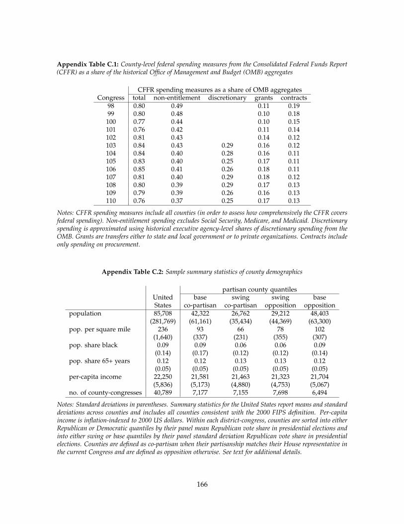
Appendix Table C.1: County-level federal spending measures from the Consolidated Federal Funds Report(CFFR) as a share of the historical Office of Management and Budget (OMB) aggregates

CFFR spending measures as a share of OMB aggregatesCongress total non-entitlement discretionary grants contracts

98 0.80 0.49 0.11 0.1999 0.80 0.48 0.10 0.18

100 0.77 0.44 0.10 0.15101 0.76 0.42 0.11 0.14102 0.81 0.43 0.14 0.12103 0.84 0.43 0.29 0.16 0.12104 0.84 0.40 0.28 0.16 0.11105 0.83 0.40 0.25 0.17 0.11106 0.85 0.41 0.26 0.18 0.11107 0.81 0.40 0.29 0.18 0.12108 0.80 0.39 0.29 0.17 0.13109 0.79 0.39 0.26 0.16 0.13110 0.76 0.37 0.25 0.17 0.13

Notes: CFFR spending measures include all counties (in order to assess how comprehensively the CFFR coversfederal spending). Non-entitlement spending excludes Social Security, Medicare, and Medicaid. Discretionaryspending is approximated using historical executive agency-level shares of discretionary spending from theOMB. Grants are transfers either to state and local government or to private organizations. Contracts includeonly spending on procurement.

Appendix Table C.2: Sample summary statistics of county demographics

partisan county quantilesUnited base swing swing baseStates co-partisan co-partisan opposition opposition

population 85,708 42,322 26,762 29,212 48,403(281,769) (61,161) (35,434) (44,369) (63,300)

pop. per square mile 236 93 66 78 102(1,640) (337) (231) (355) (307)

pop. share black 0.09 0.09 0.06 0.06 0.09(0.14) (0.17) (0.12) (0.12) (0.14)

pop. share 65+ years 0.12 0.12 0.13 0.13 0.12(0.05) (0.05) (0.05) (0.05) (0.05)

per-capita income 22,250 21,581 21,463 21,323 21,704(5,836) (5,173) (4,880) (4,753) (5,067)

no. of county-congresses 40,789 7,177 7,155 7,698 6,494

Notes: Standard deviations in parentheses. Summary statistics for the United States report means and standarddeviations across counties and includes all counties consistent with the 2000 FIPS definition. Per-capitaincome is inflation-indexed to 2000 US dollars. Within each district-congress, counties are sorted into eitherRepublican or Democratic quantiles by their panel mean Republican vote share in presidential elections andinto either swing or base quantiles by their panel standard deviation Republican vote share in presidentialelections. Counties are defined as co-partisan when their partisanship matches their House representative inthe current Congress and are defined as opposition otherwise. See text for additional details.

166

Appendix Table C.3: US House: full panel, regression discontinuity, and first-difference estimates on logper-capita federal spending under alternative partisan county quantiles

moving average panel average moving panel averagepresidential vote share House vote share House vote share

non-entitlement grants non-entitlement grants non-entitlement grantsspending spending spending spending spending spending

Panel A: Full panelco-partisan county 0.0001 0.0144 0.0104 0.0146 0.0080 0.0401**

(0.0071) (0.0088) (0.0140) (0.0160) (0.0113) (0.0176)swing county -0.0003 -0.0054 0.0100 0.0027 0.0006 0.0127

(0.0062) (0.0103) (0.0185) (0.0197) (0.0120) (0.0156)co-partisan county -0.0060 0.0047 -0.0075 0.0147 -0.0053 -0.0155×swing county (0.0077) (0.0113) (0.0131) (0.0185) (0.0136) (0.0264)

county FE X X X X X Xdistrict-congress FE X X X X X Xno. of county-congresses 28,512 28,512 17,195 17,195 10,681 10,681no. of district-congresses 2,208 2,208 1,363 1,363 852 852no. of states 47 47 47 47 46 46

Panel B: Regression discontinuityRepublican county -0.0132 -0.0006 -0.0041 0.0797 0.0192 0.0111×Republican district (0.0286) (0.0341) (0.0396) (0.0716) (0.0504) (0.0668)

county FE X X X X X Xdistrict-congress FE X X X X X Xno. of county-congresses 5,304 5,304 3,059 3,059 1,953 1,953no. of district-congresses 383 383 226 226 151 151no. of states 45 45 42 42 36 36

Panel C: First-difference∆ co-partisan county 0.0083 0.0062 -0.0013 0.0295 0.0889 0.1264

(0.0142) (0.0159) (0.0207) (0.0219) (0.0505) (0.0988)∆ swing county 0.0337*** 0.0218 -0.0256 0.0376 0.0089 0.0310

(0.0096) (0.0173) (0.0167) (0.0334) (0.0369) (0.0653)∆ (co-partisan county -0.0236 -0.0074 0.0090 -0.0365 -0.0057 0.0273×swing county) (0.0144) (0.0255) (0.0229) (0.0398) (0.0482) (0.1046)

district-congress FE X X X X X Xno. of county-congresses 3,716 3,715 1,916 1,915 265 264no. of district-congresses 350 350 313 313 25 25no. of states 37 37 37 37 10 10

Notes: Standard errors in parentheses and clustered by state. Opposition county and base county are theomitted categories in Panels A and C. Democratic county, base county, and Democratic district are the omittedcategories in Panel B. Moving average captures the average of the election returns for the current and previousfive Congresses. Panel average uses the average for the entire data set. Panel B implements the RDD by usingthe full sample to estimate the county fixed effects and by limiting a local linear regression to elections wherethe leading candidate wins by less than a 5 percentage point margin. Panel C restricts the sample to periodsbefore and after redistricting where the party of the House representative also remains the same. See text foradditional details. * - p-value < 0.10, ** - p-value < 0.05, *** - p-value < 0.01

167

Appendix Table C.4: US House: full panel estimates on spending variables divided by voter turnout

log (per-voter federal spending)total non-entitlement discretionary grants contracts

Panel A: Turnout in presidential electionsco-partisan county -0.0048 -0.0061 0.0097 0.0096 -0.0158

(0.0064) (0.0094) (0.0120) (0.0104) (0.0242)swing county 0.0069 0.0001 -0.0154 -0.0103 -0.0687*

(0.0103) (0.0166) (0.0223) (0.0150) (0.0386)co-partisan county -0.0002 0.0031 -0.0179 -0.0058 0.0517×swing county (0.0071) (0.0115) (0.0138) (0.0127) (0.0326)

county FE X X X X Xdistrict-congress FE X X X X Xno. of county-congresses 28,522 28,522 17,815 28,522 28,522no. of district-congresses 2,208 2,208 1,355 2,208 2,208no. of states 47 47 47 47 47

Panel B: Turnout in US House electionsco-partisan county 0.0042 0.0128 0.0148 0.0147

(0.0138) (0.0227) (0.0244) (0.0528)swing county 0.0112 0.0196 0.0519 0.0001

(0.0147) (0.0243) (0.0316) (0.0744)co-partisan county -0.0104 -0.0251 -0.0207 0.0059×swing county (0.0180) (0.0253) (0.0321) (0.0660)

county FE X X X Xdistrict-congress FE X X X Xno. of county-congresses 12,952 12,952 12,952 12,952no. of district-congresses 1,018 1,018 1,018 1,018no. of states 46 46 46 46

Notes: Standard errors in parentheses and clustered by state. Opposition county and base county are theomitted categories. Panel A uses presidential elections to measure voter turnout and to define the partisancounty quantiles based on panel average vote shares. Similarly, Panel B uses US House elections to measurevoter turnout and define the partisan county quantiles. The measure of turnout from presidential elections isan average of the two previous presidential elections because they only occur every other Congress. Withineach district-congress, counties are sorted into either Republican or Democratic quantiles by their panel meanvote share and into either swing or base quantiles by their panel standard deviation vote share. Counties aredefined as co-partisan when their partisanship matches their House representative in the current Congress andare defined as opposition otherwise. See text for additional details. * - p-value < 0.10, ** - p-value < 0.05, *** -p-value < 0.01

168

Appendix Table C.5: US House: regression discontinuity estimates on covariates with federal spending

Panel A: County demographicslog (total log (pop pop. share pop. share log (per-

population) per sq. mile) African-American 65+ years capita income)Republican county -0.0049 -0.0049 -0.0022 0.0004 -0.0149×Republican district (0.0140) (0.0140) (0.0015) (0.0020) (0.0095)

county FE X X X X Xdistrict-congress FE X X X X Xno. of county-congresses 5,304 5,304 5,304 5,304 5,242no. of district-congresses 383 383 383 383 383no. of states 45 45 45 45 45

Panel B: Lagged log (per-capita federal spending)total non-entitlement discretionary grants contracts

Republican county 0.0234 0.0176 0.0624 0.0466 -0.0548×Republican district (0.0256) (0.0357) (0.0520) (0.0394) (0.1027)

county FE X X X X Xdistrict-congress FE X X X X Xno. of county-congresses 4,724 4,724 2,888 4,722 4,715no. of district-congresses 342 342 198 342 342no. of states 45 45 42 45 45

Notes: Standard errors in parentheses and clustered by state. Democratic county, base county, and Democratic district are the omitted categories. Implementsthe RDD by using the full sample to estimate the county fixed effects and by limiting a local linear regression to elections where the leading candidate winsby less than a 5 percentage point margin. Per-capita income is inflation-indexed to 2000 US dollars. See text for additional details. * - p-value < 0.10, ** -p-value < 0.05, *** - p-value < 0.01

169

Appendix Table C.6: Comparison of regression discontinuity estimates on log per-capita federal spendingunder alternative bandwidths

bandwidth (in percentage points)7.5 5 2.5

Panel A: Total spendingRepublican county 0.0103 -0.0034 0.0331×Republican district (0.0186) (0.0204) (0.0244)

no. of county-congresses 7,669 5,304 2,624no. of district-congresses 570 383 195no. of states 46 45 41

Panel B: Non-entitlement spendingRepublican county -0.0058 -0.0267 0.0228×Republican district (0.0314) (0.0315) (0.0366)

no. of county-congresses 7,669 5,304 2,624no. of district-congresses 570 383 195no. of states 46 45 41

Panel C: Discretionary spendingRepublican county 0.0248 -0.0192 -0.0370×Republican district (0.0462) (0.0529) (0.0921)

no. of county-congresses 4,905 3,351 1,518no. of district-congresses 357 232 114no. of states 46 43 37

Panel D: Grants spendingRepublican county -0.0154 -0.0531 -0.0184×Republican district (0.0372) (0.0450) (0.0675)

no. of county-congresses 7,669 5,304 2,624no. of district-congresses 570 383 195no. of states 46 45 41

Panel E: Contracts spendingRepublican county -0.0976 -0.1011 -0.1014×Republican district (0.0840) (0.1043) (0.1756)

no. of county-congresses 7,669 5,304 2,624no. of district-congresses 570 383 195no. of states 46 45 41

Notes: Standard errors in parentheses and clustered by state. Dependent variable is log per-capita federalspending. Includes district-congress and county fixed effects. Implements the RDD by using the full sampleto estimate the county fixed effects and by limiting a local linear regression to elections where the leadingcandidate wins by less than either a 7.5, 5, or 2.5 percentage point margin. See text for additional details. * -p-value < 0.10, ** - p-value < 0.05, *** - p-value < 0.01

170