Essays in International FinanceThe Harvard community has made this

article openly available. Please share howthis access benefits you. Your story matters

Citation Du, Wenxin. 2013. Essays in International Finance. Doctoraldissertation, Harvard University.

Citable link http://nrs.harvard.edu/urn-3:HUL.InstRepos:12362594

Terms of Use This article was downloaded from Harvard University’s DASHrepository, and is made available under the terms and conditionsapplicable to Other Posted Material, as set forth at http://nrs.harvard.edu/urn-3:HUL.InstRepos:dash.current.terms-of-use#LAA

Essays in International Finance

A dissertation presented by

Wenxin Du

to

The Department of Economics

in partial fulfillment of the requirementsfor the degree of

Doctor of Philosophyin the subject of

Economics

Harvard UniversityCambridge, Massachusetts

May 2013

c2013 — Wenxin Du

All rights reserved.

Dissertation Advisors: John Y. Campbell, Gita Gopinath Wenxin Du

Essays in International Finance

ABSTRACT

This dissertation consists of three essays in international finance. The first two essays study

emerging market sovereign risk with a focus on local currency denominated sovereign bonds.

The third essay examines econometric tools for robust inference in the presence of missing obser-

vations, an issue frequently encountered by researchers in international finance.

Most emerging market sovereign borrowing is now denominated in local currencies. In Chap-

ter 1, we introduce a new measure of sovereign risk, the local currency credit spread, defined as the

synthetic dollar spread on a local currency bond after using cross currency swaps to hedge the cur-

rency risk of promised cash flows. Compared with traditional sovereign risk measures based on

foreign currency denominated debt, we find that local currency credit spreads have lower means,

lower cross-country correlations, and are less sensitive to global risk factors. We rationalize these

findings with a model allowing for different degrees of integration between domestic and external

debt markets.

Chapter 2 documents new empirical evidence on the rapid growth of foreign ownership of

emerging market local currency sovereign debt over the past decade. We study risk of nominal

bonds without hedging away the currency risk. We show that local currency nominal bond risks

differ across countries and are highly correlated with sovereign credit default swap spreads on

foreign currency external debt. Using data on investors’ forecasts of inflation and growth, we find

that perceived differences in the cyclicality of monetary policy help explain the cross-sectional

and time series variation in nominal bond risk as well as the development of local currency debt

markets. Guided by these observed empirical patterns, we develop a simple general equilibrium

model with an endogenous issuance decision between local and foreign currency debt.

Chapter 3 proposes two simple consistent heteroskedasticity and autocorrelation consistent co-

variance estimators for time series with missing data. First, we develop the Amplitude Modulated

iii

estimator by applying the Newey-West estimator and treating the missing observations as non-

serially correlated. Secondly, we develop the Equal Spacing estimator by applying the Newey-

West estimator to the series formed by treating the data as equally spaced. We show asymptotic

consistency of both estimators for inference purposes and discuss finite sample variance and bias

tradeoff.

iv

TABLE OF CONTENTS

Abstract . . . . . . . . . . . . . . . . . . . . . . . . . . . . . . . . . . . . . . . . . . . . . . . . . . iii

Acknowledgments . . . . . . . . . . . . . . . . . . . . . . . . . . . . . . . . . . . . . . . . . . . . . ix

1. Local Currency Sovereign Risk . . . . . . . . . . . . . . . . . . . . . . . . . . . . . . . . . . . . 11.1 Introduction . . . . . . . . . . . . . . . . . . . . . . . . . . . . . . . . . . . . . . . . . . 1

1.1.1 Relation to the Literature . . . . . . . . . . . . . . . . . . . . . . . . . . . . . . 71.2 Cross Currency Swaps and Sovereign Credit Spreads . . . . . . . . . . . . . . . . . . 8

1.2.1 Cross Currency Swaps . . . . . . . . . . . . . . . . . . . . . . . . . . . . . . . . 81.2.2 LC and FC Credit Spreads . . . . . . . . . . . . . . . . . . . . . . . . . . . . . . 9

1.3 New Stylized Facts on LC Sovereign Risk . . . . . . . . . . . . . . . . . . . . . . . . . 121.3.1 Deviations from Long-Term CIP . . . . . . . . . . . . . . . . . . . . . . . . . . 121.3.2 Mean Levels of Credit Spreads . . . . . . . . . . . . . . . . . . . . . . . . . . . 161.3.3 Widening Credit Spread Differentials During the Crisis . . . . . . . . . . . . . 191.3.4 Cross-Country Correlations of Credit Spreads . . . . . . . . . . . . . . . . . . 201.3.5 Correlation of Sovereign Risk with Global Risk Factors . . . . . . . . . . . . . 221.3.6 Summary of Stylized Facts . . . . . . . . . . . . . . . . . . . . . . . . . . . . . 25

1.4 A No-Arbitrage Model with Risky Credit Arbitrage . . . . . . . . . . . . . . . . . . . 261.4.1 Differential Cash Flow Risk and Investor Bases . . . . . . . . . . . . . . . . . . 261.4.2 Environment . . . . . . . . . . . . . . . . . . . . . . . . . . . . . . . . . . . . . 281.4.3 Pricing FC and LC Bonds . . . . . . . . . . . . . . . . . . . . . . . . . . . . . . 291.4.4 Comparative Statics . . . . . . . . . . . . . . . . . . . . . . . . . . . . . . . . . 321.4.5 Empirical Decomposition of Credit Spread Differentials . . . . . . . . . . . . 35

1.5 Differential Risk Premia . . . . . . . . . . . . . . . . . . . . . . . . . . . . . . . . . . . 371.5.1 Benchmark Regressions . . . . . . . . . . . . . . . . . . . . . . . . . . . . . . . 371.5.2 Cross-Country Variation . . . . . . . . . . . . . . . . . . . . . . . . . . . . . . . 411.5.3 Excess Returns Predictability . . . . . . . . . . . . . . . . . . . . . . . . . . . . 44

1.6 Conclusion . . . . . . . . . . . . . . . . . . . . . . . . . . . . . . . . . . . . . . . . . . . 47

2. The End of“Original Sin”: Nominal Bond Risk in Emerging Markets . . . . . . . . . . . . . . . 492.1 Introduction . . . . . . . . . . . . . . . . . . . . . . . . . . . . . . . . . . . . . . . . . . 492.2 Related Literature . . . . . . . . . . . . . . . . . . . . . . . . . . . . . . . . . . . . . . . 522.3 The End of “Original Sin” . . . . . . . . . . . . . . . . . . . . . . . . . . . . . . . . . . 542.4 Measuring Nominal Bond Risks . . . . . . . . . . . . . . . . . . . . . . . . . . . . . . . 59

2.4.1 Definition of Nominal Bond Betas . . . . . . . . . . . . . . . . . . . . . . . . . 592.4.2 Cross-country Variations in Nominal Bond Risk . . . . . . . . . . . . . . . . . 61

2.5 What Explains Nominal Bond Risk? . . . . . . . . . . . . . . . . . . . . . . . . . . . . 642.5.1 Bond Betas and Sovereign CDS Spreads . . . . . . . . . . . . . . . . . . . . . 642.5.2 Cyclicality of Inflation Expectation . . . . . . . . . . . . . . . . . . . . . . . . . 65

v

2.6 Implications of Nominal Risk on Sovereign Portfolios . . . . . . . . . . . . . . . . . . 672.7 General Equilibrium Model of Sovereign Portfolio Choice . . . . . . . . . . . . . . . . 69

2.7.1 Theoretical Framework . . . . . . . . . . . . . . . . . . . . . . . . . . . . . . . 692.7.2 Second Period Problem . . . . . . . . . . . . . . . . . . . . . . . . . . . . . . . 702.7.3 First Period Problem: External Debt Only . . . . . . . . . . . . . . . . . . . . . 75

2.8 Conclusion . . . . . . . . . . . . . . . . . . . . . . . . . . . . . . . . . . . . . . . . . . . 83

3. Nonparametric HAC Estimation for Time Series Data with Missing Observations . . . . . . . . 843.1 Introduction . . . . . . . . . . . . . . . . . . . . . . . . . . . . . . . . . . . . . . . . . . 84

3.1.1 Relation to the Literature . . . . . . . . . . . . . . . . . . . . . . . . . . . . . . 873.2 A simple example . . . . . . . . . . . . . . . . . . . . . . . . . . . . . . . . . . . . . . . 893.3 Long-Run Variance of Time Series with Missing Observations . . . . . . . . . . . . . 92

3.3.1 Missing Data Structure . . . . . . . . . . . . . . . . . . . . . . . . . . . . . . . 923.3.2 Newey-West Estimator . . . . . . . . . . . . . . . . . . . . . . . . . . . . . . . 933.3.3 Long-Run Variance of the Underlying Process - Parzen Estimator . . . . . . . 943.3.4 Long-Run Variance of the Observed Process . . . . . . . . . . . . . . . . . . . 953.3.5 Finite Samples . . . . . . . . . . . . . . . . . . . . . . . . . . . . . . . . . . . . . 99

3.4 Regression Model with Missing Observations . . . . . . . . . . . . . . . . . . . . . . . 1013.5 Simulation . . . . . . . . . . . . . . . . . . . . . . . . . . . . . . . . . . . . . . . . . . . 103

3.5.1 Data Structure . . . . . . . . . . . . . . . . . . . . . . . . . . . . . . . . . . . . . 1043.5.2 Evaluation Criteria . . . . . . . . . . . . . . . . . . . . . . . . . . . . . . . . . . 1063.5.3 Results . . . . . . . . . . . . . . . . . . . . . . . . . . . . . . . . . . . . . . . . . 108

3.6 Empirical Application: Recursive Tests for a Positive Sample Mean . . . . . . . . . . 1163.7 Conclusion . . . . . . . . . . . . . . . . . . . . . . . . . . . . . . . . . . . . . . . . . . . 124

Appendix 125

A. Appendix to Chapter 1 . . . . . . . . . . . . . . . . . . . . . . . . . . . . . . . . . . . . . . . . 126A.1 A Real-World Example . . . . . . . . . . . . . . . . . . . . . . . . . . . . . . . . . . . . 126A.2 Yield Curve Construction . . . . . . . . . . . . . . . . . . . . . . . . . . . . . . . . . . 126A.3 N-Period Extension . . . . . . . . . . . . . . . . . . . . . . . . . . . . . . . . . . . . . . 128

A.3.1 Risk-Free Rates . . . . . . . . . . . . . . . . . . . . . . . . . . . . . . . . . . . . 128A.3.2 FC Bonds . . . . . . . . . . . . . . . . . . . . . . . . . . . . . . . . . . . . . . . 128A.3.3 LC Bonds . . . . . . . . . . . . . . . . . . . . . . . . . . . . . . . . . . . . . . . 129

Bibliography . . . . . . . . . . . . . . . . . . . . . . . . . . . . . . . . . . . . . . . . . . . . . . . . 135

vi

LIST OF TABLES

1.1 Mean LC and FC Credit Spread Comparison, 2005-2011. . . . . . . . . . . . . . . . . 181.2 Changes in Credit Spreads During Crisis Peak (09/01/08 - 09/01/09). . . . . . . . . 201.3 Cross-Country Correlation of Credit Spreads, 2005-2011. . . . . . . . . . . . . . . . . 211.4 Cross-Country Correlation of Credit Spreads, 2005-2011. . . . . . . . . . . . . . . . . 221.5 Regressions of Bond Excess Returns on Equity Returns, 2005-2011. . . . . . . . . . . 251.6 Regression of 5-Year Credit Spreads on VIX, 2005m1-2011m12. . . . . . . . . . . . . . 401.7 Impact of VIX on Credit Spreads by Country. . . . . . . . . . . . . . . . . . . . . . . . 431.8 Forecasting Quarterly Holding-Period Excess Returns, 2005m1-2011m12. . . . . . . . 46

2.1 Equity and Bond Excess Return Correlation with U.S. Markets (2005-2012). . . . . . . 622.2 Fixed Coupon LC Debt as a Fraction of Domestic Debt. . . . . . . . . . . . . . . . . . 682.3 Fixed Coupon LC Debt as a Fraction of Total Sovereign Debt. . . . . . . . . . . . . . . 69

3.1 Daily Gasoline Prices. . . . . . . . . . . . . . . . . . . . . . . . . . . . . . . . . . . . . . 903.2 Daily Gasoline Prices with Missing Observations. . . . . . . . . . . . . . . . . . . . . 913.3 Benchmark Results. . . . . . . . . . . . . . . . . . . . . . . . . . . . . . . . . . . . . . . 1083.4 Varying Missing Structure. . . . . . . . . . . . . . . . . . . . . . . . . . . . . . . . . . . 1093.5 Finite Samples: Fixed and Automatic Bandwidth Selection. . . . . . . . . . . . . . . . 1113.6 Empirical Bias and Variance. . . . . . . . . . . . . . . . . . . . . . . . . . . . . . . . . . 1123.7 Automatically Selected Bandwidths. . . . . . . . . . . . . . . . . . . . . . . . . . . . . 1143.8 Varying Fraction of Missings. . . . . . . . . . . . . . . . . . . . . . . . . . . . . . . . . 1153.9 Rejection Rates for Recursive Tests. . . . . . . . . . . . . . . . . . . . . . . . . . . . . . 120

A.1 Cross-Currency Swaps and Currency Forward Comparison, 2005-2011. . . . . . . . . 132A.2 Half of Bid-ask Spreads on FX Spots, Forwards and Swaps, 2005-2011. . . . . . . . . 133A.3 Data Sources and Variable Construction. . . . . . . . . . . . . . . . . . . . . . . . . . . 134

vii

LIST OF FIGURES

1.1 Offshore Trading Volume by Instrument Types (Trillions of USD). . . . . . . . . . . . 31.2 Cumulative Flows of Offshore Emerging Market Funds (Billions of USD) . . . . . . . 41.3 5-Year U.S. and Swapped UK Treasury Yields in percentage points. . . . . . . . . . . 121.4 5-Year Swapped LC and FC Spreads in percentage points. . . . . . . . . . . . . . . . . 141.4 (Continued) 5-Year Swapped LC and FC Spreads in percentage points. . . . . . . . . 151.5 Brazil Onshore and Offshore Yield Comparison. . . . . . . . . . . . . . . . . . . . . . 171.6 Swapped LC over FC spreads. . . . . . . . . . . . . . . . . . . . . . . . . . . . . . . . . 191.7 5-Year Sovereign Credit Spreads in Italy. . . . . . . . . . . . . . . . . . . . . . . . . . . 361.8 5-Year Sovereign Credit Spreads in Russia. . . . . . . . . . . . . . . . . . . . . . . . . 361.9 Differential Risk Aversion Pass-Though and Return Correlation. . . . . . . . . . . . . 42

2.1 Foreign Ownership of Government Debt in Emerging and Developed Markets. . . . 552.2 Time Series of Foreign Ownership of Government Debt in Emerging Markets. . . . . 562.3 Ownership of Domestic Debt by Security Type in 2012. . . . . . . . . . . . . . . . . . 572.4 Ownership Structure of Peruvian Nominal Bonds (millions of nuevo soles). . . . . . 582.5 Local, Global and Currency Betas (2005-2012). . . . . . . . . . . . . . . . . . . . . . . 632.6 Bond Betas and Sovereign CDS Spreads. . . . . . . . . . . . . . . . . . . . . . . . . . . 652.7 Forecast Beta and Bond Beta. . . . . . . . . . . . . . . . . . . . . . . . . . . . . . . . . 662.8 Inflation and Default Policy Functions. . . . . . . . . . . . . . . . . . . . . . . . . . . . 752.9 Share of LC Debt vs. Amount of Revenue Raised. . . . . . . . . . . . . . . . . . . . . 772.10 Expected Inflation and Default for Equilibrium Portfolios. . . . . . . . . . . . . . . . 782.11 The Role of Risk Premium. . . . . . . . . . . . . . . . . . . . . . . . . . . . . . . . . . . 802.12 Share of LC External Financing with Endogenous Output. . . . . . . . . . . . . . . . 822.13 Inflation and Default with Domestic Financing. . . . . . . . . . . . . . . . . . . . . . . 82

3.1 Time Series of Returns. . . . . . . . . . . . . . . . . . . . . . . . . . . . . . . . . . . . . 1213.2 Recursive Test Results - Sample Mean and Error Bands. . . . . . . . . . . . . . . . . . 1223.3 Backwards Recursive Test Results - Sample Mean and Error Bands. . . . . . . . . . . 123

A.1 An Illustration of Swap Covered Local Currency Investment. . . . . . . . . . . . . . . 131

viii

ACKNOWLEDGMENTS

I owe sincere and earnest thankfulness to my thesis advisors John Y. Campbell, Gita Gopinath

and Luis M. Viceira for their invaluable help and guidance. I cannot thank John enough for being

a conscientious mentor and role model, who has inspired and nurtured my interests in financial

economics. I am tremendously grateful to Gita for nurturing my scholarship over years, and

going above and beyond for me throughout the job market process. This work would not have

been possible without her brilliance and generosity of time and resources. I am also extremely

thankful to Luis for his constant enthusiasm and encouragement. His knowledge and insights

have been indispensable for all my progress.

I am grateful to James Stock and Rustam Ibragimov for their insightful guidance in draft-

ing Chapter 3 of this dissertation. I am also grateful to my co-authors Jesse Schreger and Deepa

Dhume Datta. Their inspiration and dedication have been instrumental to the quality of my work.

I also thank Javier Bianchi, Fernando Broner, Gary Chamberlain, Emmanuel Farhi, Jeffrey

Frankel, Jeffry Frieden, Robin Greenwood. Ricardo Hausman, Jakub Jurek, Sebnem Kalemli-

Ozcan, Hanno Lustig, Matteo Maggiori, Ulrich Mueller, Jose Luis Montiel, Michael Rashes, Ken-

neth Rogoff, Jeremy Stein, Adrien Verdelhan and seminar participants at AQR Capital Manage-

ment, Federal Reserve Board, Harvard, Maryland, NBER IFM Meeting, Stanford GSB, UCLA An-

derson, Penn Wharton, UCSD, UVA Darden and World Bank for comments and suggestions. I

thank Harvard Graduate Student Fellowship and the International Economics Grant for provid-

ing financial support for my research.

I deeply appreciate my friends and fellow classmates, Jisoo Hwang and Anitha Sivasankaran

with whom I seldom talk economics, for being able to share in all the joys and challenges of

graduate school and life. On the subject of graduate school life, I owe much to Brenda Piquet.

Everything would not be as seamless without her support.

I am indebted to my best friends from Swarthmore, Qing Ling, Bo Hu and Yijun Li, for spend-

ing countless hours helping me find the right data, sharing their perspectives as financial practi-

ix

tioners in investment banks, and even more importantly, for their continual love and emotional

support.

Finally, I would like to dedicate this dissertation to my parents, Xiaojun Ding and Xiaoqing

Du, simply for their unconditional love and support from thousands of miles away over the years.

Also, I hope that my husband Yafeng Li, will continue to bring out the best in me.

x

1. LOCAL CURRENCY SOVEREIGN RISK1

1.1 Introduction

In the aftermath of the Global Financial Crisis, sovereign debt crises are concentrated in the

developed world. This itself is a remarkable development. It is even more remarkable when

one considers that following the Lehman bankruptcy, some emerging market currencies lost more

than half their value against the dollar. Yet even as their currencies plummeted, these countries

were able to continue their debt payments. This represents a major break from past crises. In the

1980’s and 1990’s the developing world borrowed in currencies that they did not have the right

to print, and currency mismatch was the center of past emerging market sovereign crises.2 After

a decade of rapid development of local currency (LC) sovereign bond markets in the wake of the

Asian Financial Crisis, major emerging markets entered the most recent period of global financial

turmoil with an increasing fraction of their debt in their own currencies and have weathered the

shocks without triggering major sovereign debt crises.3

Yet, despite the increasingly important role of local currency debt in emerging market gov-

ernment finance, LC debt markets are little understood and LC sovereign risk measures are ab-

sent from the academic literature. Our paper fills this gap by introducing a new measure of LC

sovereign risk, the LC credit spread, defined as the difference between the nominal yield on an LC

bond and the LC risk-free rate implied from the cross currency swap (CCS) market. While gov-

ernment bond yields are often used directly as the risk-free rate for developed country currencies,

they cannot be used as the risk-free rate in emerging markets where the risk of sovereign default

1 Joint with Jesse Schreger, Harvard University

2 Prominent examples are Mexico (1994), the Asian Financial Crises (1997-98), Russia (1998), Brazil (1998, 2002),Turkey (2000-01) and Argentina (2001-02).

3 Sovereign defaults have occurred in four developing countries since 2008: Ecuador, Seychelles, Jamaica and Belize.Except for Jamaica, the other three countries do not have local currency debt markets. Ecuador is a fully dollarizedeconomy and Seychelles and Belize have population less than 500,000.

1

and capital controls are non-negligible.4 Instead, we use the dollar risk-free rate combined with

the long-term forward rate implied from the currency swap markets as the risk-free benchmark in

each LC. From a dollar investor’s perspective, the LC credit spread is equivalent to the synthetic

dollar spread on an LC bond over the U.S. Treasury rate with the currency risk of promised cash

flows fully hedged using cross currency swaps. By holding an LC bond and a currency swap with

the same tenor and promised cash flows, the dollar investor can lock in the LC credit spread even

if the value of the currency plummets as long as explicit default is avoided. From the sovereign

issuer’s perspective, the LC credit spread measures the synthetic dollar borrowing cost in the LC

debt market.

The bulk of the literature on emerging market LC debt has focused on why these emerging

markets cannot borrow abroad in their own currency, the question of “original sin” surveyed in

Eichengreen and Hausmann (2005). While it is true that emerging market sovereigns rarely issue

LC bonds in global markets, this no longer means that foreigners do not lend to them in their own

currencies. Instead foreigners are increasingly willing to purchase LC debt issued under domestic

law. According to volume surveys conducted by the Emerging Market Trading Association, the

share of LC debt in total offshore emerging market debt trading volume has increased from 35

percent in 2000 to 71 percent in 2011, reaching 4.64 trillion U.S. dollars (Figure 1.1). Emerging

Market Portfolio Research reports that even among offshore mutual funds which had historically

invested overwhelmingly in FC denominated Eurobonds5 and Brady bonds, the cumulative fund

flow into LC emerging market debt securities has outpaced the flow into debt securities in hard

currencies (Figure 1.2).

The growing importance of LC debt markets is in stark contrast to the declining role of FC

sovereign financing. This shift is rendering conventional measures of sovereign risk increasingly

obsolete. In many emerging markets, government policy is to retire outstanding FC debt and end

new FC issuance.6 The popular country-level JP Morgan Emerging Market Bond Index (EMBI),

commonly used in academic research to measure sovereign risk, is today forced to track a dwin-

4 A similar point applies to many euro area countries.

5 Throughout this paper we use eurobonds to mean foreign currency bonds issued offshore, but not necessarily ineuros.

6 For example in Mexico, the 2008 guidelines for public debt management is to “Continue emphasis on the use ofdomestic debt to finance the entire federal government deficit and the stock of external debt” (SHCP, 2008)

2

0.00

1.00

2.00

3.00

4.00

5.00

6.00

7.00

8.00

2000 2001 2002 2003 2004 2005 2006 2007 2008 2009 2010 2011

Volu

me

in T

rilli

ons

of U

SD

Brady, Options, Loans FC Bonds LC Bonds

Figure 1.1: Offshore Trading Volume by Instrument Types (Trillions of USD). This figure plots total trad-ing volumes of emerging market debt by instrument type in trillions of dollars. In addition toFC bonds, the ‘Brady, Option, Loans” category also refers to debt instruments denominated inforeign currencies. The survey participants consist of large offshore financial institutions.Source: Annual Debt Trading Volume Survey (2000-2011) by Emerging Market Trading Associ-ation

dling number of outstanding FC eurobonds with declining liquidity and trading volume. In coun-

tries such as Egypt, Thailand, Malaysia, Morocco, South Korea and Qatar, FC debt has shrunk

to the point that EMBI+ has been forced to discontinue these countries’ indices. In addition to

FC credit spreads, sovereign CDS spreads are used as an alternative measure of sovereign risk.

However, defaults on local currency bonds governed under domestic law do not constitute credit

events that trigger CDS contracts in emerging markets.7 As a result, sovereign CDS also offers an

incomplete characterization of emerging market sovereign risk.

Using new data and a new measure, we document a new set of stylized facts about LC sovereign

risk. To construct LC and FC sovereign credit spreads, we build a new dataset of zero-coupon LC

and FC yield curves and swap rates for 10 major emerging markets at the daily frequency for a

common sample period from 2005 to 2011. Using the 5-year zero-coupon benchmark, we find that

LC credit spreads are significantly above zero, robust to taking into account the bid-ask spread

on the swap rates. This result demonstrates the failure of long-term covered interest rate par-

ity between government bond yields in emerging markets and the United States. Removing the

7 This is different from the case of developed country sovereign CDS for which a default on local bonds would triggerCDS contracts (ISDA, 2012).

3

-10

10

30

50

70

90

110

2005m1 2006m1 2007m1 2008m1 2009m1 2010m1 2011m1 2012m1

Billi

ons

of U

SD

Blend Fund FC Fund LC Fund

Figure 1.2: Cumulative Flows of Offshore Emerging Market Funds (Billions of USD). This figure plotscumulative flows of offshore mutual funds designated to emerging market debt since 2005, mea-sured in billions of USD. Monthly fund flow is measured as end-of-month assets - beginning-of-month assets - portfolio change - FX change. The total cumulative flow is broken down bycurrency type. LC Fund refers to funds that invest 75 percent or more in local currency debt;FC Fund refers to funds that invest 75 or more in hard currency debt; and Blend Fund refers tofunds that invest in a combination of both, less than 75 percent for either of the above categories.Source: Emerging Market Portfolio Research

currency risk highlights an important credit component in LC yields, as shown by the positive

correlation between the LC credit spread and the conventional sovereign risk measure, the FC

credit spread.

Despite a positive correlation, LC and FC credit spreads are different along three important di-

mensions. First, while LC credit spreads are large and economically significant, they are generally

lower than FC credit spreads. The gap between LC and FC credit spreads significantly widened

during the peak of the crisis following the Lehman bankruptcy. Second, FC credit spreads are

much more correlated across countries than LC credit spreads. Over 80% of the variation in FC

spreads is explained by the first principal component. In contrast, only 53% of the variation in

LC credit spreads is explained by the first principal component, pointing to the relative impor-

tance of country-specific factors in driving LC spreads. Third, FC credit spreads are much more

correlated with global risk factors than are LC credit spreads. These ex-ante results in the yield

spread space are mirrored ex-post in the excess return space, as excess holding period returns on

FC bonds over U.S. Treasuries load heavily on global equity market returns while hedged LC ex-

4

cess holding period returns load heavily on local equity market returns. In other words, despite

the common perception of emerging market LC debt as extremely risky, we find that swapped LC

debt is actually safer than FC bonds for global investors measured in terms of global equity betas.

The removal of currency risk is central to this finding, as the currency unhedged LC excess returns

have larger betas with global equity returns than FC excess returns.

After documenting the differences between LC and FC credit spreads, we turn to examining

the sources of these credit spread differentials. We build a parsimonious model that attributes the

credit spread differential to the differential cash flow risks between LC and FC debt and differen-

tial investor bases between the two debt markets. FC bonds may have higher cash flow risk than

LC for several reasons. These include a government’s option to print money to service LC debt,

the danger that a sudden exchange rate depreciation may increase the real burden of servicing FC

debt, and the political economy costs of defaulting on your own citizens relative to defaulting on

foreign investors. On the other hand, foreign holders of LC debt face several risks not present in

FC eurobonds, including convertibility risk, as well as the risks of changing taxation and regula-

tion and more uncertain debt restructuring process under the domestic law. In addition, LC and

FC credit spreads can be different due to unhedged covariance between the exchange rate and the

default process. From a dollar investor’s perspective, swapped LC debt can have lower cash flow

risk if investors expect to gain profits from unwinding the swap position in the event of an LC

bond default.

In addition to differential cash flow risk, LC and FC debt markets have different investor bases.

While an increasing fraction of LC debt is being purchased by foreign investors, the majority is still

owned by domestic residents, commercial banks, and pension funds. These investors have few

investment opportunities outside of domestic government bonds because of domestic financial

underdevelopment or legal restrictions on their overseas investments. This can give rise to a

distinct local demand factor in pricing LC debt that is absent from FC debt, which is issued in

major international capital markets and purchased by diversified global investors. The existence

of local clientele potentially dampens the sensitivity of LC credit spreads to fundamentals and

global investor risk aversion shocks.

We study a model that allows for both differential cash flow risk and local clientele demand ef-

fects by introducing credit risk in the style of of Duffie and Singleton (1999) into a preferred habitat

5

model that builds on Greenwood and Vayanos (2010) and Vayanos and Vila (2009). While allow-

ing the arrival rate of credit events for FC and LC to respond differently to a local and global risk

factor, we study a market structure where diversified global investors are the primary clientele for

FC debt, domestic investors are the primarily clientele for LC debt, and risk-averse arbitrageurs

partially integrate the two markets. In this framework, the equilibrium LC credit spread is an

endogenous outcome of arbitrageurs’ optimal portfolio demand and local clientele demand, with

the equilibrium impact of LC clientele demand depending on on the size of the position the arbi-

trageur is willing to take. This, in turn, depends on the arbitrageur’s risk aversion, the asset return

correlation, and the size and elasticity of local clientele demand.

Guided by the model’s predictions and comparative statics, we highlight the importance of

differential risk premia arising from the differential investor bases in pricing swapped LC and FC

bonds. The key mechanism we highlight is how changes in global risk aversion directly affect

FC spreads but are only partially transmitted into LC spreads by risk-averse arbitrageurs. Con-

sistent with the model’s predictions, we first show that global risk aversion, as proxied by VIX,

has a larger contemporaneous impact on FC credit spreads than on LC credit spreads, robust to

a large set of determinants of sovereign risk identified by the existing literature. Differential sen-

sitivity to VIX alone accounts for 25.6 percent of the within-country variation in the credit spread

differentials and 60 percent of total explained variation after controlling for a host of economic

fundamentals. Furthermore, differential contemporaneous impacts of VIX on LC and FC credit

spreads generate differential predictability of excess returns through the risk premium channel.

We show that high levels of VIX significantly forecast negative swapped LC over FC excess re-

turns. As predicted by the theory, we also find that LC credit spreads are more sensitive to global

risk aversion in countries with more correlated swapped LC and FC bond returns.

The paper is structured as follows. We begin by explaining this paper’s place in the existing

literature. Section 1.2 explains the mechanics of cross currency swaps and formally introduces the

LC credit spread measure. Section 1.3 presents new stylized facts on LC sovereign risk. Section

1.4 lays out a no-arbitrage model of partially segmented markets with risky credit arbitrage. Sec-

tion 1.5 performs regression analysis to test several key predictions of the model and Section 1.6

concludes.

6

1.1.1 Relation to the Literature

Our work is related to several distinct strands of literature: the enormous sovereign debt litera-

ture in international macroeconomics, the empirical sovereign and currency risk premia literature,

the literature on currency-specific corporate credit spreads, and the segmented market asset pric-

ing literature.

Recent work by Carmen Reinhart and Kenneth Rogoff demonstrates (Reinhart and Rogoff

2008, 2011) that LC sovereign borrowing and default are not new phenomena. Building on their

work, which focuses primarily on quantities, we focus on prices and jointly examine LC and FC

credit spreads. Prior to our work, the pricing of LC debt was rarely examined with exception

of Burger and Warnock (2007) and Burger, Warnock, and Warnock (2012), who studied ex-post

returns on LC bonds using the J.P. Morgan Emerging Market Government Bond Index (EM-GBI)

index.

Using our dataset of daily yield curves and currency swaps, we document a series of new styl-

ized facts that we believe are important to integrate into the quantitative sovereign debt literature

that builds on Aguiar and Gopinath (2006) and Arellano (2008). Given that an increasing fraction

of sovereign borrowing is in LC, our findings on how LC credit spreads behave differently than

FC credit spreads highlight the importance of moving away from the standard assumption in this

literature that governments borrow solely from foreign lenders using real debt.

Our paper is also closely related to the literature on FC sovereign risk premia and currency risk

premia. Borri and Verdelhan (2011) demonstrate that FC spreads can be explained by modeling a

risk-averse investor who demands risk premia for holding sovereign debt because default gener-

ally occurs during bad times for the global investors. Using data on credit default swaps (CDS)

denominated in dollars, Longstaff, Pan, Pedersen, and Singleton (2011) show that global risk fac-

tors explain more of the variation in CDS spreads than do local factors. Our analysis confirms

these findings. In addition, we find support for the results of Lustig and Verdelhan (2007) and

Lustig, Roussanov, and Verdelhan (2012) that there is a common global factor in currency returns.

This motivates our use of cross currency swaps to separate this currency risk from the credit risk

on LC sovereign debt.

7

Cross currency swaps have previously been used to test long-term covered interest parity

among government bond yields in developed countries. Popper (1993) and Fletcher and Taylor

(1994, 1996) document some deviations from covered parity, but they are an order of magnitude

smaller and much less persistent than those we document in our dataset of emerging markets.

Currency-dependent credit spreads implied from cross currency swaps have also received atten-

tion in the empirical corporate finance literature. McBrady and Schill (2007) demonstrate that

firms gauge credit spread differentials across different currencies when choosing the currency

denomination of their debt. Jankowitsch and Stefan (2005) highlight the role of the correlation

between FX and default risk in affecting currency-specific credit spreads. Lowenkron and Garcia

(2005) document that currency and credit risk, the so-called “cousin risk”, are positively linked in

some emerging markets, but not in others.

Finally, our theoretical model builds on the asset pricing literature on investors’ preferred

habitats and the limits to arbitrage. Greenwood and Vayanos (2010), building on Vayanos and

Vila (2009), examine the effect of increases in bond supply across the yield curve for U.S. Trea-

suries. The framework assumes that different maturities have different clienteles and each type of

investor invests only in a certain range of maturities (their “preferred habitat”). We study an en-

vironment where preferred habitats correspond to currencies and markets rather than maturities,

building on the cross-asset arbitrage theory presented by Gromb and Vayanos (2010), and solving

analytically for the endogenous LC bond price.

1.2 Cross Currency Swaps and Sovereign Credit Spreads

1.2.1 Cross Currency Swaps

For short-term instruments, FX forward contracts allow investors to purchase foreign exchange

at pre-determined forward rates. Beyond one year, liquidity is scarce in the forward markets and

long-term currency hedging via forwards is very costly. CCS contracts, on the other hand, allow

investors to conveniently hedge long-term currency risk. A CCS is an interest rate derivative con-

tract that allows two parties to exchange interest payments and principal denominated in two

currencies. A real-world example of hedging currency risk of an LC bond using CCS is given

in Appendix A.1. For emerging markets, CCS counterparties are usually large offshore financial

8

institutions. To mitigate the counterparty risk embedded in CCS contracts, the common market

practice is to follow the Credit Support Annex of the International Swap and Derivative Associa-

tion Master Agreement, which requires bilateral collateralization of CCS positions, and thus coun-

terparty risk is fairly negligible. For countries with non-deliverable FX forwards, CCS contracts

are cash settled in dollars based on LC notional amount and are free from currency convertibility

risk.

For our cross-country study, it is cumbersome to deal with coupon bearing bonds and par

swap rates due to the mismatch in coupon rates and payment dates between bonds and swaps.

We can extract the long-term FX forward premium (the zero-coupon swap rate) implicit in the

term structure of par swaps. Intuitively, a fixed for fixed LC/dollar CCS package can always be

considered as the sum of two interest rate swaps. First, the investor swaps the fixed LC cash flow

into a floating U.S. Libor cash flow8 and then swaps the floating U.S. Libor cash flow into a fixed

dollar cash flow. We can exploit the fact that the receiver of U.S. Libor must be indifferent between

offering a fixed LC or a fixed dollar cash flow. The difference in the two swap rates thus implies

the long-term currency view of the financial market. After performing this transformation, a CCS

is completely analogous to a standard forward contract. The specifics are given in the following

proposition.

Proposition 1. Given implied log spot rates rLCτ,t from the fixed LC for U.S. Libor CCS and rUSD

τ,t from the

fixed dollar for Libor interest rate swap, the implicit long-term forward premium is equal to

ρnt ≡1τ( fnt − st) = rLC

nt − rUSDnt ,

where fn is the pre-determined log forward exchange rate at which a transaction between LC and dollars

takes place n years ahead.

1.2.2 LC and FC Credit Spreads

The core of our dataset is daily zero-coupon yield curves and swap curves for LC and FC

sovereign bonds issued by 10 different emerging market governments from January, 2005 to De-

8 For Mexico, Hungary, Israel and Poland in our sample, this step itself combines two interest rate swaps: an onshoreplain vanilla LC fixed for LC floating interest rate swap and a cross-currency LC floating for U.S. Libor basis swap.

9

cember, 2011. We use a benchmark tenor of 5 years. The choice of countries is mainly constrained

by the lack of sufficient numbers of FC bonds outstanding. Furthermore, all 10 sample countries

belong to the J.P. Morgan EM-GBI index, an investable index for emerging market LC bonds. The

length of the sample period is constrained by the availability of long-term currency swap data.

All data on cross currency swaps are collected from Bloomberg.9 Zero coupon yield curves are

collected or estimated from various data sources. The details on the yield curve construction are

given in Appendix A.2.

We work with log yields throughout the paper. To fix notations, we let y∗nt denote the n-year

zero-coupon U.S. Treasury bond yield, the long-term risk-free rate used throughout the paper.

Nominal LC and FC yields are denoted by yLCnt and yFC

nt , respectively. We let ρnt denote the zero-

coupon swap rate, the implicit forward premium as defined in Proposition 1. All yields and swap

rates are for the n-year zero-coupon benchmark at date t. The conventional measure of sovereign

risk, the FC credit spread, measures the difference between the yield on FC debt and the U.S.

Treasury yield:

sFC/USnt = yFC

nt − y∗nt.

Our new measure for LC sovereign risk, the LC credit spread, is defined as the nominal LC spread

over the the U.S. Treasury yield, minus the zero-coupon swap rate:

sSLC/USnt = yLC

nt − y∗nt − ρnt,

or the deviation from long-term covered interest rate parity between the government bond yields.

There are two ways to interpret this measure. First, the dollar investor can create a swapped LC

bond by combining an LC bond with a CCS with the same promised cash flows. The synthetic

9 Extremely illiquid trading days with bid-ask spreads over 400 basis points on CCS are excluded from the analysis(mainly for Indonesia during the 2008 crisis). All main results are not affected by including these extreme values. Wecompare the difference in 1-year forward premia implied by the swap and the forward markets in Table A.1. The meancorrelation is 99 percent. Using annualized bid-ask spreads as a proxy for liquidity,swap contracts are, on average,more liquid than short-term forward contracts (Table A.2) .

10

dollar yield on the swapped LC bond is given by

ySLCnt = yLC

nt − ρnt.

The LC credit spread is therefore equal to the dollar spread on this synthetic asset:

sSLC/USnt = (yLC

nt − ρnt)− y∗nt = ySLCnt − y∗nt.

Hence, by holding the swapped LC bond to maturity, the LC credit spread gives the promised

dollar spread on the LC bond to dollar investors even if the LC depreciates, provided that explicit

default is avoided. In the event of default, the dollar investor can choose to unwind the swap

with an unmatched LC bond payment, which could result in additional FX profits or losses from

the swap. Second, investors valuing their returns in LC can combine a U.S. Treasury bond with

a fixed for fixed CCS to create an LC risk-free bond. The sum of the dollar risk-free and the CCS

rate gives the LC risk free rate

y∗LCnt = y∗nt + ρnt,

and thus the LC credit spread measures the yield spread of the LC bond over the LC risk-free rate:

sSLC/USnt = yLC

nt − (y∗nt + ρnt) = yLCnt − y∗LC

nt ,

and is a pure credit spread measure for local currency. Finally, the LC over FC credit spread

differential measures the spread between the yield on the synthetic dollar asset combining an LC

bond and CCS over the FC bond yield:

sSLC/FCnt = yLC

nt − ρnt − yFCnt = sSLC/US

nt − sFC/USnt .

From the issuer’s perspective, it gives the the difference between the synthetic dollar borrowing

cost in the local market and the actual dollar borrowing cost in the external market.

11

1.3 New Stylized Facts on LC Sovereign Risk

1.3.1 Deviations from Long-Term CIP

If long-term covered interest parity holds for government bond yields, LC credit spreads

should equal zero in the absence of transaction costs. As a starting point, Figure 1.3 plots the

5-year swapped UK Treasury yield in dollars and the U.S. Treasury yield from 2000 to 2011. The

difference between the two curves, the UK LC credit spread, averages 10 basis points for the

full sample and 6 basis points excluding 2008-2009. Long-term CIP holds quite well between the

U.S. and the UK Treasury yields excluding 2008-2009. At the peak of the Global Financial Crisis

around the Lehman bankruptcy, the UK credit spread temporarily increased to 100 basis points

but returned to normal in a few months.

02

46

8

2000 2001 2002 2003 2004 2005 2006 2007 2008 2009 2010 2011 2012

US yield Swapped UK dollar yield

Swapped UK/US dollar spread

Figure 1.3: 5-Year U.S. and Swapped UK Treasury Yields in percentage points. The green solid line plotsthe 5-Year zero-coupon U.S. Treasury yield. The blue dash-dotted line plots the 5-year zero-coupon swapped UK Treasury yield after applying a cross currency swap package consistingof two plain vanilla interest rate swaps (dollar and sterling) and the U.S. and UK Libor cross-currency basis swap. The orange dashed line plots the yield spread of the swapped UK Treasuryyield over the U.S. Treasury. The mean of the yield spreads is 10 basis points with standarddeviation equal to 16 basis points. The minimum spread is equal to negative 25 basis pointsand the maximum spread is equal to 106 basis points during the peak of the crisis. Excluding2008-2009, the mean spread is 6 basis points with standard deviation equal to 10 basis points.Source: The U.S. zero-coupon yield is from St. Louis Fed. The UK zero-coupon yield is fromBank of England. Swap rates are from Bloomberg.

12

LC credit spreads in emerging markets offer a very different picture. As can be seen in Fig-

ure 1.4, where the 5-year zero-coupon yield spreads are plotted for our sample countries, large

persistent deviations from long-term covered interest parity are the norm rather than the excep-

tion. Column 1 in Table 1.1 presents summary statistics for 5-year LC spreads for the sample

period 2005-2011 at daily frequency. LC credit spreads, sSLC/US, have a cross-country mean of

128 basis points, calculated using the mid-rates on the swaps. Brazil records the highest mean

LC spreads equal to 313 basis points and Mexico and Peru have the lowest means about 60 basis

points. All mean LC credit spreads are positive and statistically significantly different from zero

using Newey-West standard errors allowing for heteroskedasticity and serial correlation.10 Pos-

itive mean LC spreads are robust to taking into account the transaction costs of carrying out the

swaps. Column 4 provides summary statistics for liquidity of the cross currency swaps, baCCS/2,

defined as half of the bid-ask spread of cross currency swap rates, with the sample average equal

to 19 basis points. We perform statistical tests and find that LC credit spreads remain significantly

positive for every country after subtracting one half of the bid-ask spread on the CCS in order to

incorporate the transaction costs. Positive LC credit spreads suggest that emerging market nom-

inal LC sovereign bonds are not free from credit risk from the investor’s perspective. Although

the government has the option to print the domestic currency, inflation is not costless and explicit

repudiation of LC debt has happened in the past, such as Russia’s default on its Treasury bills in

1998.

10 Following Datta and Du (2012), missing data are treated as non-serially correlated for Newey-West implementa-tions throughout the paper.

13

03

69

12

15

2005 2006 2007 2008 2009 2010 2011 2012

LC/US

FC/US

Zero−Coupon Swap Rate

Swapped LC/US

Brazil 5Y

03

69

12

15

2005 2006 2007 2008 2009 2010 2011 2012

LC/US

FC/US

Zero−Coupon Swap Rate

Swapped LC/US

Colombia 5Y

03

69

12

15

2005 2006 2007 2008 2009 2010 2011 2012

LC/US

FC/US

Zero−Coupon Swap Rate

Swapped LC/US

Hungary 5Y

03

69

12

15

2005 2006 2007 2008 2009 2010 2011 2012

LC/US

FC/US

Zero−Coupon Swap Rate

Swapped LC/US

Indonesia 5Y

03

69

12

15

2005 2006 2007 2008 2009 2010 2011 2012

LC/US

FC/US

Zero−Coupon Swap Rate

Swapped LC/US

Israel 5Y

03

69

12

15

2005 2006 2007 2008 2009 2010 2011 2012

LC/US

FC/US

Zero−Coupon Swap Rate

Swapped LC/US

Mexico 5Y

Figure 1.4: 5-Year U.S. and Swapped UK Treasury Yields in percentage points. Each figure plots 10-daymoving averages of zero-coupon LC and FC spreads over the U.S. Treasury at 5 years. LC/USdenotes the LC yield over the U.S. Treasury yield. FC/US denotes the FC yield over the U.S.Treasury yield. Zero-coupon swap rate is the zero-coupon fixed for fixed CCS rate implied frompar fixed for floating CCS and plain vanilla interest rate swap rates. Swapped LC/US denotesthe swapped LC over U.S. Treasury yield spread.

14

03

69

12

15

2005 2006 2007 2008 2009 2010 2011 2012

LC/US

FC/US

Zero−Coupon Swap Rate

Swapped LC/US

Peru 5Y

03

69

12

15

2005 2006 2007 2008 2009 2010 2011 2012

LC/US

FC/US

Zero−Coupon Swap Rate

Swapped LC/US

Philippines 5Y

03

69

12

15

2005 2006 2007 2008 2009 2010 2011 2012

LC/US

FC/US

Zero−Coupon Swap Rate

Swapped LC/US

Poland 5Y

03

69

12

15

2005 2006 2007 2008 2009 2010 2011 2012

LC/US

FC/US

Zero−Coupon Swap Rate

Swapped LC/US

Turkey 5Y

Figure 1.4: (Continued) 5-Year U.S. and Swapped UK Treasury Yields in percentage points. Each figureplots 10-day moving averages of zero-coupon LC and FC spreads over the U.S. Treasury at 5years. LC/US denotes the LC yield over the U.S. Treasury yield. FC/US denotes the FC yieldover the U.S. Treasury yield. Zero-coupon swap rate is the zero-coupon fixed for fixed CCS rateimplied from par fixed for floating CCS and plain vanilla interest rate swap rates. SwappedLC/US denotes the swapped LC over U.S. Treasury yield spread.

15

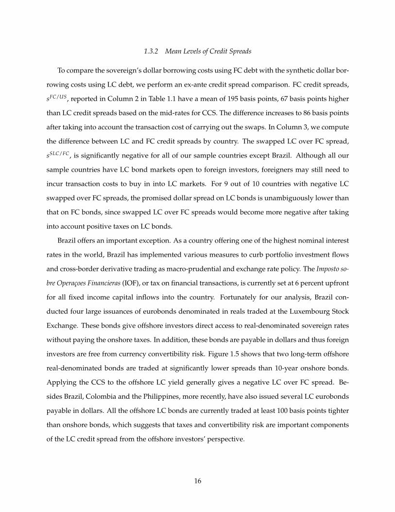
1.3.2 Mean Levels of Credit Spreads

To compare the sovereign’s dollar borrowing costs using FC debt with the synthetic dollar bor-

rowing costs using LC debt, we perform an ex-ante credit spread comparison. FC credit spreads,

sFC/US, reported in Column 2 in Table 1.1 have a mean of 195 basis points, 67 basis points higher

than LC credit spreads based on the mid-rates for CCS. The difference increases to 86 basis points

after taking into account the transaction cost of carrying out the swaps. In Column 3, we compute

the difference between LC and FC credit spreads by country. The swapped LC over FC spread,

sSLC/FC, is significantly negative for all of our sample countries except Brazil. Although all our

sample countries have LC bond markets open to foreign investors, foreigners may still need to

incur transaction costs to buy in into LC markets. For 9 out of 10 countries with negative LC

swapped over FC spreads, the promised dollar spread on LC bonds is unambiguously lower than

that on FC bonds, since swapped LC over FC spreads would become more negative after taking

into account positive taxes on LC bonds.

Brazil offers an important exception. As a country offering one of the highest nominal interest

rates in the world, Brazil has implemented various measures to curb portfolio investment flows

and cross-border derivative trading as macro-prudential and exchange rate policy. The Imposto so-

bre Operaçoes Financieras (IOF), or tax on financial transactions, is currently set at 6 percent upfront

for all fixed income capital inflows into the country. Fortunately for our analysis, Brazil con-

ducted four large issuances of eurobonds denominated in reals traded at the Luxembourg Stock

Exchange. These bonds give offshore investors direct access to real-denominated sovereign rates

without paying the onshore taxes. In addition, these bonds are payable in dollars and thus foreign

investors are free from currency convertibility risk. Figure 1.5 shows that two long-term offshore

real-denominated bonds are traded at significantly lower spreads than 10-year onshore bonds.

Applying the CCS to the offshore LC yield generally gives a negative LC over FC spread. Be-

sides Brazil, Colombia and the Philippines, more recently, have also issued several LC eurobonds

payable in dollars. All the offshore LC bonds are currently traded at least 100 basis points tighter

than onshore bonds, which suggests that taxes and convertibility risk are important components

of the LC credit spread from the offshore investors’ perspective.

16

02

46

2007 2008 2009 2010 2011 2012

Onshore 10Y Swapped LC/US 10Y FC/US

Offshore BRL 2022−10Y CCS Offshore BRL 2028−10Y CCS

Figure 1.5: Brazil Onshore and Offshore Yield Comparison. This figure plots nominal yields minus 10-yearzero-coupon real/dollar swap rates on two Eurobonds denominated in Brazilian reals traded atthe Luxembourg Stock Exchange with maturity years 2022 and 2028 (BRL 2022 by the green long-dashed line and BRL 2028 by the blue short-dashed line). Offshore swapped yields are comparedwith the 10-year zero-coupon onshore LC swapped yield plotted by the orange dash-dotted lineand the offshore FC dollar yield plotted by the red solid line.Source: The onshore LC zero-coupon yield is obtained from ANBIMA. The FC zero-couponyield is estimated from Bloomberg BFV par yield curve. LC Eurobond yields are provided bythe Luxembourg Stock Exchange.

Despite the level difference in credit spreads, one might expect LC and FC credit risks to be

correlated within countries, as in downturns a country could find it more tempting to explicitly

default on both types of debt. Column 5 confirms this conjecture. The within-country correla-

tion between LC and FC credit spreads is positive for every country with a mean of 54 percent.

However, there is significant cross-country heterogeneity. The correlation is highest for Hungary

at 91% and lowest for Indonesia at 18%. This cross-country heterogeneity is a source of variation

that we will later use to argue for the importance of incomplete market integration in the relative

pricing of the two types of debt.

17

Table 1.1: Mean LC and FC Credit Spread Comparison, 2005-2011. This table reports sample starting date,mean and standard deviation of 5-year log yield spreads at daily frequency. The variables are(1) sSLC/US, swapped LC over U.S. Treasury spread; (2) sFC/US, FC over U.S. Treasury spread; (3)sSLC/FC , swapped LC over FC spread, or column (2) - column (1). (4) baCCS/2 , half of bid-askspread of cross-currency swaps. Standard deviations of the variables are reported in the parenthe-ses. We test significance of means using Newey-West standard errors with 120-day lags. Standarderrors are omitted. Test results are reported for columns (1), (2) and (3), *** p<0.01, ** p<0.05, *p<0.1. Since the bid-ask spread is always nonnegative, significance tests are not performed forcolumn 4. Two additional tests are conducted for hypotheses (1) sSLC/US − baCCS/2 = 0 andsSLC/FC − baCCS/2/2 = 0, both tests can be rejected at 5 percent or lower confidence levels forall countries using Newey-West standard errors with 120-day lags. Column (5) reports within-country correlations between sSLC/US and sFC/US.

Sample (1) (2) (3) (4) (5)Country Start sSLC/US sFC/US sSLC/FC baCCS/2 Corr(SLC,FC)

Brazil Jul. 2006 3.13*** 1.78*** 1.35*** 0.32 0.56(1.13) (0.91) (0.94) (0.13)

Colombia Jun. 2005 1.47*** 2.03*** -0.56*** 0.16 0.34(0.69) (1.01) (1.01) (0.10)

Hungary Jan. 2005 1.69*** 2.15*** -0.47** 0.19 0.91(1.23) (2.01) (1.03) (0.14)

Indonesia Apr. 2005 1.14*** 2.52*** -1.38*** 0.38 0.18(0.73) (1.59) (1.61) (0.23)

Israel Feb. 2006 0.86*** 1.12*** -0.26*** 0.12 0.84(0.43) (0.42) (0.21) (0.03)

Mexico Jan. 2005 0.60*** 1.44*** -0.83*** 0.09 0.66(0.40) (0.79) (0.60) (0.06)

Peru Jul. 2006 0.55*** 1.97*** -1.42*** 0.16 0.34(0.80) (1.05) (1.09) (0.07)

Philippines Mar. 2005 1.25*** 2.31*** -1.07*** 0.28 0.34(0.80) (1.04) (1.07) (0.14)

Poland Mar. 2005 1.04*** 1.29*** -0.25** 0.12 0.78(0.60) (1.01) (0.62) (0.08)

Turkey May 2005 1.46*** 2.57*** -1.12*** 0.11 0.78(1.19) (1.20) (0.81) (0.08)

Total Jan. 2005 1.28*** 1.95*** -0.67*** 0.19 0.54(1.06) (1.23) (1.22) (0.15)

Observations 13151 13151 13151 13151

18

1.3.3 Widening Credit Spread Differentials During the Crisis

Despite the relatively short sample period, the years 2005-2011 cover dynamic world economic

events: the end of the great moderation, the Global Financial Crisis and the subsequent recovery.

Figure 1.6 plots the difference in LC and FC credit spreads, sSLC/FC, across 10 countries over the

sample period. While swapped LC over FC spreads largely remain in negative territory (with the

exception of Brazil), the spreads significantly widened during the peak of the crisis following the

Lehman bankruptcy. The maximum difference between LC and FC credit spreads for any country

during the crisis was negative 10 percentage points for Indonesia.

−10

−5

05

2005 2006 2007 2008 2009 2010 2011 2012

Brazil Colombia Hungary Indonesia Israel

Mexico Peru Philippines Poland Turkey

Figure 1.6: Swapped LC over FC spreads. This figure plots 30-day moving averages of 5-year zero-couponswapped LC over FC spreads (the difference between LC and FC credit spreads) using 5-yearcross currency swaps for all 10 sample countries.

Table 1.2 quantitatively documents the behavior of the credit spreads during the crisis peak

(defined approximately as the year following the Lehman bankruptcy from September 2008 to

September 2009), measured as the increase in spreads relative to their pre-crisis means. FC credit

spreads significantly increase in all countries and LC credit spreads increase significantly in 8 out

of the 10 sample countries, with the exceptions of Indonesia and Peru. However, the increase

in swapped LC spreads are generally less than the increase in FC spreads, as LC over FC credit

spread differentials are reduced for all countries except Brazil. The divergent behavior of these

19

credit spreads during the crisis peak highlights significant differences between LC and FC bonds,

and offers a key stylized fact to be examined in Sections 1.4 and 1.5.

Table 1.2: Changes in Credit Spreads During Crisis Peak (09/01/08 - 09/01/09). This table reports the meanand standard deviation of changes in LC and FC credit spreads during the peak of the GlobalFinancial Crisis (09/01/2008-09/01/2009) relative to their pre-crisis means. (1) ∆sSLC/US is theincrease in swapped LC over U.S. Treasury spreads; (2) ∆sFC/US is the increase in the FC overU.S. Treasury spreads; (3) ∆sSLC/FC is the increase in swapped LC over FC spreads, or column (2)-column (1); and (4) ∆baCCS/2 is the increase in one half of bid-ask spreads. Standard deviationsof variables are reported in the parentheses. Statistical significance of the means are tested usingNewey-West standard errors with 120-day lags. Significance levels are denoted by *** p<0.01, **p<0.05, * p<0.1.

(1) (2) (3) (4)Country ∆sSLC/US ∆sFC/US ∆sSLC/FC ∆baCCS/2

Brazil 1.93*** 1.82*** 0.11 0.26***(1.13) (0.99) (0.66) (0.13)

Colombia 0.64*** 2.31*** -1.66*** 0.10***(0.67) (1.21) (0.82) (0.18)

Hungary 2.70*** 3.80*** -1.10** 0.31***(1.12) (2.17) (1.48) (0.22)

Indonesia 0.07 3.67*** -3.61*** 0.45***(0.65) (2.17) (2.41) (0.39)

Israel 0.54*** 0.68*** -0.15*** 0.05***(0.26) (0.26) (0.21) (0.04)

Mexico 0.60*** 1.97*** -1.38*** -0.03***(0.30) (0.87) (0.80) (0.01)

Peru -0.05 2.21*** -2.26*** 0.07***(0.95) (1.12) (0.81) (0.08)

Philippines 0.36*** 1.91*** -1.55*** 0.18***(0.40) (1.28) (1.33) (0.22)

Poland 1.26*** 2.35*** -1.09*** 0.17***(0.58) (0.92) (1.01) (0.09)

Turkey 1.89*** 2.70*** -0.81*** -0.06***(1.44) (1.47) (0.86) (0.07)

Total 0.91*** 2.30*** -1.40*** 0.14***(1.16) (1.48) (1.51) (0.22)

Observations 2058 2058 2058 2058

1.3.4 Cross-Country Correlations of Credit Spreads

In Table 1.3, we conduct a principal component (PC) analysis to determine the extent to which

fluctuations in the LC and FC credit spreads are driven by common components or by idiosyn-

cratic country shocks. In the first column, we see that the first principal component explains less

than 54% of the variation in LC credit spreads across countries. This is in sharp contrast to the FC

20

Table 1.3: Cross-Country Correlation of Credit Spreads, 2005-2011. This table reports summary statistics ofprincipal component analysis and cross-country correlation matrices of monthly 5-Year LC and FCcredit spreads and sovereign credit default swap spreads. The variables are (1) sSLC/US, swappedLC over U.S. Treasury spreads; (2) sFC/US, FC over U.S. Treasury spreads; (3) 5Y CDS five-yearsovereign CDS spreads. The rows “First”, “Second”, “Third” report percentage and cumulativepercentage of total variations explained by the first, second and third principal components, re-spectively. The row“Pairwise Corr.” reports the mean of all bilateral correlations for all countrypairs. All variables are end-of-the-month observations.

(1) (2) (3)Principal sSLC/US sFC/US 5Y CDS

Components percentage total percentage total percentage total

First 53.49 53.49 81.52 81.52 80.02 80.02Second 16.30 69.78 11.70 93.22 15.34 95.36Third 10.17 79.95 3.68 96.90 2.06 97.41

Pairwise Corr. 0.42 0.78 0.77

spreads (Column 2) where over 81% of total variation is explained by the first PC. The first three

principal components explain slightly less than 80% of the total variation for LC credit spreads

whereas for FC credit spreads they explain about 97%. In addition, we find that the average pair-

wise correlation of LC credit spreads between countries is only 42%, in contrast to 78% for FC

credit spreads. These findings point to country-specific idiosyncratic components as important

drivers of LC credit spreads, in contrast to the FC market where global factors are by far the most

important.11

To link these results to the literature using CDS spreads as a measure of sovereign risk, we

perform the same principal component analysis for 5-year sovereign CDS spreads. The results, in

Column 3, are very similar to the FC results in Column 2: the first principal component explains

80 percent of total variation of CDS spreads and the pairwise correlation averages 77 percent. Our

result that an overwhelming amount of the variation in CDS spreads is explained by the first PC

supports the finding of Longstaff, Pan, Pedersen, and Singleton (2011), which shows that 64% of

CDS spreads are explained by the first principal component of 26 developed and emerging mar-

11 To assess how measurement errors in LC credit spreads relative to FC affect these results, we start with the nullhypothesis that LC and FC credit spreads are the same and then introduce i.i.d. Gaussian shocks to FC credit spreadsusing simulations. We show that the variance of shocks to FC credit spreads need to be at least 90 basis points to matchthe observed cross-country correlation in LC credit spreads, which corresponds to 6 times of the standard deviation ofobserved one-way transaction costs (half of the observed bid-ask spread on cross currency swaps). These simulationresults are available upon request.

21

kets. The sample period for their study is 2000-2010, but the authors find in the crisis subsample

of 2007-2010 that the first principal component accounts for 75% of the variation.

1.3.5 Correlation of Sovereign Risk with Global Risk Factors

Credit Spreads

After identifying an important global component in both LC and FC credit spreads, we now

try to understand what exactly this first principal component is capturing. In Table 1.4, we first

examine the correlation of the first PC’s of credit spreads with each other and with global risk

factors. The global risk factors include the Merrill Lynch U.S. BBB corporate bond spread over

the Treasuries, BBB/T, the implied volatility on S&P options, VIX, and the Chicago Fed National

Activity Index, CFNAI, which is the first PC of 85 monthly real economic indicators. Panel (A)

indicates that the first PC of FC credit spreads has remarkably high correlations with these three

global risk factors, 93% with VIX, 88% with BBB/T and 76% with global macro fundamentals

(or, more precisely, US fundamentals) proxied by the CFNAI index. The correlation between the

first PC of LC credit spreads and global risk factors are lower, but still substantial, with a 76%

correlation with VIX, 71% with BBB/T and 57% with CFNAI.

Table 1.4: Cross-Country Correlation of Credit Spreads, 2005-2011. This table reports correlations amongcredit spreads and global risk factors. Panel (A) reports correlations between the first principalcomponent of credit spreads and global risk factors. Panel (B) reports average correlations be-tween raw credit spreads in 10 sample countries and global risk factors. Panel (C) reports corre-lations between global risk factors only. The three credit spreads are (1) sSLC/US, 5-year swappedLC over U.S. Treasury spread; (2) sFC/US, 5-year FC over U.S. Treasury spread; and (3) 5Y CDS,5-year sovereign credit default swap spread. The three global risk factors are (1)BBB/T, MerrillLynch BBB over 10-year Treasury spread; (2) -CFNAI, negative of the real-time Chicago Fed Na-tional Activity Index, or the first principal component of 85 monthly economic indicators (positiveCFNAI indicates improvement in macroeconomic fundamentals), and (3) VIX, implied volatilityon the S&P index options. All variables use end-of-the-month observations.

(A) First PC of Credit Spreads (B) Raw Credit Spreads (C) Global Risk FactorssSLC/US sFC/US 5Y CDS sSLC/US sFC/US 5Y CDS BBB/T -CFNAI VIX

sSLC/US 1.00 1.00sFC/US 0.81 1.00 0.49 1.005Y CDS 0.80 0.94 1.00 0.48 0.91 1.00BBB/T 0.71 0.88 0.89 0.38 0.66 0.62 1.00

-CFNAI 0.57 0.76 0.75 0.33 0.58 0.52 0.87 1.00VIX 0.76 0.93 0.87 0.41 0.70 0.61 0.80 0.68 1.00

22

Furthermore, since the first PC explains much more variation in FC credit spreads than in LC

credit spreads, the cross-country average correlation between raw credit spreads and global risk

factors is much higher for FC than for LC debt (Panel B). Notably, VIX has a mean correlation of

70 percent with FC credit spreads, but only 41 percent with LC credit spreads. This leads us to

conclude that the observed global factors are more important in driving spreads on FC debt than

on swapped LC debt. Unsurprisingly, the correlations between the global factors and the CDS

spread are very similar to the correlations between these factors and the FC spread.

Excess Returns

Having examined the ex-ante promised yields in Tables 1.3 and 1.4, we next turn to ex-post

realized returns. The natural measures to study are the excess returns of LC and FC bonds over

U.S. Treasury bonds. In particular, we run a series of beta regressions to examine how LC and FC

excess returns vary with global and local equity markets. Before turning to these results, we first

define the different types of returns. Since all yields spreads are for zero-coupon benchmarks, we

can quickly compute various excess returns for the holding period ∆t.12 The FC over US excess

holding period return for an n-year FC bond is equal to

rxFC/USn,t+∆t = nsFC/US

nt − (n − ∆t)sFC/USn−∆t,t+∆t,

which represents the change in the log price of the FC bond over a U.S. Treasury bond of the same

maturity. Similarly, the currency-specific return differential of an LC bond over a U.S. Treasury

bond is given by

rxLC/USn,t+∆t = nsLC/US

nt − (n − ∆t)sLC/USn−∆t,t+∆t.

Depending on the specific FX hedging strategies, we can translate rxLC/USn,t+∆t into three types of dollar

excess returns on LC bonds. First, the unhedged LC over US excess return, uhrxLC/USn,t+∆t , is equal to

the currency-specific return differential minus the ex-post LC depreciation:

uhrxLC/USn,t+∆t = rxLC/US

n,t+∆t − (st+∆t − st),

12 For quarterly returns, ∆t is a quarter and we approximate sn−∆t,t+∆t with sn,t+∆t.

23

where st denotes the log spot exchange rate. Second, the holding-period hedged LC over US excess

return, hrxLC/USn,t+∆t , is equal to the currency-specific return differential minus the ex-ante holding

period forward premium:

hrxLC/USn,t+∆t = rxLC/US

n,t+∆t − ( ft,t+∆t − st),

where ft,t+∆t denotes the log forward rate at t for carrying out FX forward transaction ∆t ahead.

Third, swapped LC over US excess returns, srxLC/USn,t+∆t , is equal to the currency-specific return dif-

ferential minus the return on the currency swap:

srxLC/USn,t+∆t = rxLC/US

n,t+∆t − [nρnt − (n − ∆t)ρn−∆t,t+∆t].

All three LC excess returns share the same component measuring the LC and US currency-specific

return differential. Depending on the specific FX hedging strategy, the ex-post LC depreciation, ex-

ante holding period forward premium and ex-post return on the currency swap affect unhedged,

hedged and swapped excess returns, respectively.13

Table 1.5 presents panel regression results for excess bond returns over local and global equity

excess returns. Global equity excess returns are defined as the quarterly return on the S&P 500

index over 3 month U.S. Treasury bills. We define two measures of LC equity excess returns

(holding-period hedged and long-term swapped) so that a foreign investor hedging her currency

risk in the local equity market has the same degree of hedging on her bond position. We find that

FC excess returns have significantly positive betas on both global and hedged LC equity returns,

with the loading on S&P being greater. Hedged and swapped LC excess returns do not load on

the S&P, but have a significantly positive beta on local equity returns. In contrast, FX unhedged

LC excess returns have positive betas on both the S&P and local equity returns.

We therefore conclude that, for foreign investors, the main risk of LC bonds is that emerging

market currencies depreciate when returns on global equities are low. This supports the results of

Lustig, Roussanov, and Verdelhan (2011) that common factors are important drivers of currency

13 The hedged excess return is a first-order approximation of the mark-to-market (MTM) dollar return on money mar-ket hedging strategy by combining the LC bond with a long position in the domestic risk-free rate and a short positionin the dollar risk-free rate over the U.S. Treasury bond. The swapped excess return is the first order approximation ofthe MTM dollar return on the bond and the CCS over the U.S. Treasury bond. The hedging notional is equal to theinitial market value of the LC bond and is dynamically rebalanced. All the empirical results of the paper are robust tousing the exact MTM accounting for the quarterly holding period.

24

Table 1.5: Regressions of Bond Excess Returns on Equity Returns, 2005-2011.This table reports contempo-raneous betas of bond quarterly excess returns on global and local equity excess returns. The de-pendent variables are (1) and (4) rxFC/US, FC over U.S. Treasury bond excess returns; (2) hrxLC/US,hedged LC over U.S. Treasury bond excess return using 3-month forward contracts; (3) and (6)uhrxLC/US, unhedged LC over U.S. Treasury bond excess returns; and (5) srxLC/US, swapped LCover U.S. Treasury bond excess returns All excess returns are computed based on the quarterlyholding period returns on 5-year zero-coupon benchmarks (annualized). The independent vari-ables are S&P $rx, quarterly return on the S&P 500 index over 3-month U.S. T-bills; LC equityhedged $rx, quarterly return on local MSCI index hedged using 3-month FX forward over 3-monthU.S. T-bills; and LC equity swapped $rx, quarterly return on local MSCI index combined with a 5-year CCS over 3-month U.S. T-bills; All regressions are run at daily frequency with country fixedeffects using Newey-West standard errors with 120-day lags and clustering by date followingDriscoll and Kraay (1998). Significance levels are denoted by *** p<0.01, ** p<0.05, * p<0.1.

(1) (2) (3) (4) (5) (6)rxFC/US hrxLC/US uhrxLC/US rxFC/US srxLC/US uhrxLC/US

S&P $rx 0.17*** -0.023 0.26*** 0.22*** 0.0011 0.42***(0.060) (0.057) (0.081) (0.055) (0.025) (0.086)

LC equity hedged $rx 0.11*** 0.21*** 0.33***(0.036) (0.036) (0.049)

LC equity swapped $rx 0.066*** 0.099*** 0.19***(0.022) (0.021) (0.047)

Observations 12,122 12,122 12,122 12,122 12,122 12,122R-squared 0.485 0.314 0.498 0.438 0.159 0.416

returns. Our new result, however, is that once currency risk is removed, LC debt appears to be

much less risky than FC debt in the sense that it has significantly lower loadings on global equity

returns than FC debt.

1.3.6 Summary of Stylized Facts

We briefly summarize the results of Section 1.3. We first establish that emerging markets are

paying positive spreads over the risk-free rate on their LC sovereign borrowing. This result indi-

cates the failure of long-term covered interest parity for government bond yields between our ten

emerging markets and the United States. With the mean LC credit spread equal to 128 basis points,

the failure is so large as to make clear the importance of credit risk on LC debt, rather than only

pointing to a temporary deviation from an arbitrage relationship as documented in developed

markets. Positive within-country correlations between LC credit spreads and the conventional

measure of sovereign risk, FC credit spreads, also highlight the role of sovereign risk on LC debt.

25

Despite the positive correlation, LC and FC credit spreads differ along three important di-

mensions. First, while LC credit spreads are large and economically significant, they are gen-

erally lower than FC credit spreads. The difference between LC and FC credit spreads signifi-

cantly widened during the peak of the crisis following the Lehman bankruptcy. Second, FC credit

spreads are much more correlated across countries than LC credit spreads. Over 80% of the vari-

ation in FC spreads is explained by the first principal component. In contrast, only 53% of the

variation in LC credit spreads is explained by the first principal component, pointing to the rel-

ative importance of country-specific factors in driving LC spreads. Third, FC credit spreads are

much more correlated with global risk factors than LC credit spreads. We find that FC spreads are

very strongly correlated with global risk factors, including a remarkable 93% correlation between

the first PC of FC credit spreads and VIX. These results are mirrored in the return space, as excess

holding period returns on FC debt load heavily on global equity returns while excess returns on

swapped LC debt do not load on global equity returns once local equity returns are controlled.

The differences between LC and FC credit spreads have important implications. Given the

fact that the bulk of emerging market sovereign borrowing takes the form of LC debt, conven-

tional measures of sovereign risk based on FC credit spreads and CDS spreads no longer fully

characterize the costs of sovereign borrowing, the cross-country dependence of sovereign risk,

and sensitivities of sovereign spreads to global risk factors. Understanding why LC and FC credit

spreads differ is the main focus of the next two sections.

1.4 A No-Arbitrage Model with Risky Credit Arbitrage

1.4.1 Differential Cash Flow Risk and Investor Bases

Having documented a series of new stylized facts on the differential behavior of LC and FC

credit spreads, we now turn to explaining them. One natural explanation for the credit spread

differential is that swapped LC and FC bonds have differential cash flow risks. First, the sovereign

may have differential incentives to repay the debt. Since FC debt is mainly held by global investors

whereas LC bonds are mainly held by local pension funds and commercial banks, the government

may be more inclined default on FC obligations. On the other hand, if the sovereign cares more

26

about reputational costs among international creditors and the access to global capital markets,

they may have more incentive to default on local creditors.

Second, in terms of capacity to repay, sovereigns can print local currency and collect most of

their revenue in local currency. During periods of sharp exchange rate depreciation, it is easier for

the sovereigns to service LC debt than FC debt. However, given that LC debt now represents the

bulk of sovereign borrowing, defaulting on LC debt can be a more effective way to reduce debt

burden.

Third, since nearly all LC debt is issued under domestic law, LC debt is subject to the risk of

changing taxation, regulation, and custody risk, as well as a more uncertain bankruptcy proce-

dure. Offshore investors also face convertibility risk whereby a government prevents the repa-

triation of funds by introducing capital controls while avoiding technical default. FC bonds, on

the other hand, are predominantly governed under international law and are therefore free from

withholding taxes and from local government regulations.

Finally, even if the two types of debt always have the same recovery of face value upon de-

fault, there could potentially exist a wedge between credit spreads depending on FX depreciation

upon default. From a dollar investor’s perspective, when default on LC debt occurs, the investor

holding the swapped LC debt can unwind the swap contract with an unmatched LC principal

payment. This might result in additional profits in the swap position if the spot exchange rate de-

preciates relative to the ex-ante forward exchange rate upon default. On the other hand, if the spot

exchange rate depreciates upon default less than the ex-ante forward exchange rate, there would

be additional loss on the swap position. The covariance between default and FX risk is referred to

as the quanto adjustment.14

In addition to differential cash flow risk, the differential investor bases in domestic and ex-

ternal debt markets can also matter for the relative pricing of the two types of debt. FC bonds

are issued offshore,mainly targeting global investors. Although there has been increasing foreign

ownership in LC debt markets, the bulk of the LC debt is still held by local investors, such as

local pension funds, insurance companies, commercial banks and other government agencies. In

14 To remove the covariance term, the investor would need to enter a currency swap contract with a floating notionallinked to the LC bond payment (or a quanto swap). However, since EM LC bonds are not deliverable, LC credit linkedquanto swaps are rarely quoted in the market.

27

emerging markets, these domestic entires are often required by law to hold a large fraction of their

portfolios in LC treasury bonds, which gives rise a distinct local clientele demand that is absent

from the external debt market.15 This local clientele demand can have equilibrium impacts in the

presence of frictions that create limits to arbitrage.

1.4.2 Environment

We formalize a parsimonious model allowing for different degrees of market integration via

risky credit arbitrage. The model builds on the preferred habitat framework presented in Vayanos

and Vila (2009), Greenwood and Vayanos (2010) and Hamilton and Wu (2012), and surveyed in

Gromb and Vayanos (2010). Following Duffie and Singleton (1999), we take a reduced form ap-

proach to model arrival rates of credit events and allow them to depend on a local and a global

factor. We introduce partial market segmentation through three main building blocks. First, we as-

sume that FC bonds are priced by risk-averse diversified global investors with a complete-market

stochastic discount factor (SDF) that only depends on the global factor. Global risk aversion shocks

affect FC credit spreads directly through FC bonds’ systematic exposure to the global shock. Sec-

ond, we allow for the existence of local clientele demand, modeled as downward sloping outside

demand with respect to the price of swapped LC bonds. Third, we assume that a risk-averse

credit arbitrageur integrates LC and FC markets by equalizing the price of risk across the two

markets adjusting for the onshore and offshore pricing wedge. As a result, the equilibrium LC

credit spread is an endogenous outcome of the arbitrageurs’ optimal portfolio demand and local

clientele demand. The equilibrium impact of the risky arbitrage depends the size of the position

the arbitrageur is willing to take, which in turn depends on the arbitrageur’s risk aversion, the

asset return correlation, and the size and elasticity of local clientele demand.

We begin by specifying a reduced form default process for the bonds. We define νi as the time

when bonds of type j = LC, FC issued by country i default, and the conditional survival intensity,

Ii,jt+1 as the probability that the bond does not default in period t + 1 conditional on the fact that it

has not yet defaulted by period t. We let the survival intensity for bond j in country i depend on

15 Kumara and Pfau (2011) document stringent caps faced by emerging market pension funds in investing in localequities and overseas assets.

28

localzi

t

and global (zwt ) factors:

Ii,jt+1 = P(νj

i > t + 1|νji > t) = exp[−(λi,j

0 + λjczi

t + λjwzw

t + σjλcξ i

t+1 + σjλwξw

t+1)].

For simplicity, we assume zero-recovery upon default. The local and global factors follow two

AR(1) processes:

zit+1 = ςc + φczi

t + ξ it+1

zwt+1 = ςw + φwzw

t + ξwt+1,

where ξwt+1 and ξ i

t+1 are independent standard normal innovations, ςc and ςw are AR(1) drifts, and

φc and φw are the autoregressive coefficients. We interpret an increase in the factors as worsening

macroeconomic fundamentals that make default more likely. The global SDF is given by

− log Mt+1 = −m∗t+1 = ψ0 − ψzw

t − γξwt+1,

where γ indicates the risk aversion of global investors. The one-period risk-free rate is therefore

y∗1t = − log Et(Mt+1) = ψ0 − ψzwt − γ2/2.

1.4.3 Pricing FC and LC Bonds

In the case of one period bonds when defaulted bonds have zero recovery rates, the survival

process fully determines the bond returns. The variance of one-period log returns for bond j is

equal to (σj1)

2 ≡ (σjλc)

2 + (σjλw)

2. Given the global SDF and the one-period survival rate, the

one-period log FC spread over the risk-free rate is given by

sFC1t = − log Et(Mt+1 Ii,FC

t+1 )− y∗1t = λFC0 + λFC

w zwt + λFC

c zit − (σFC

1 )2/2 + γσFCλw .

The first set of terms λFC0 + λFC

c zit + λFC

w zwt is the expected default loss of the bond conditional on

the factors. The term (σFC1 )2/2 is the Jensen’s inequality correction from working with log yields.

The third term is the risk premium on the FC bond. When σλw > 0, defaults are more likely in

29

the bad states of the world for the global investor, leading the FC bond to carry a positive risk

premium due to its systematic exposure to global shocks. This is the empirically relevant case as

demonstrated in Borri and Verdelhan (2011).

Now suppose that the local bond market has an outside clientele demand, i.e., local pension

funds, and there are risk-averse arbitrageurs who arbitrage between LC and FC markets. The

arbitrageurs take the FC spread priced by the global investor as given. The LC credit spread is an

equilibrium outcome of arbitrageurs’ portfolio demand and local clientele demand. Assume that

the arbitrageurs have power utility over next-period wealth with constant relative risk aversion

γa. As demonstrated in Campbell and Viceira (2002), the first-order condition of an arbitrageur’s

optimal portfolio decision is given by

Etr1t+1 − y∗1t +12

σ2t = γaVαt

where r1t+1 is a column vector of one-period log returns of the swapped LC and FC bonds, σ2t is

the variance of log excess returns, V is the variance-covariance matrix of log excess returns, and

αt is a column vector with the arbitrageur’s portfolio weights in LC and FC debt.

We conjecture that the LC credit spread sSLC/US1t is affine in the local and global factors zi

t and

zwt and is given by

sSLC/US1t = (b10 + λSLC

0 − σ2SLC/2) + (b1c + λSLC

c )zit + (b1w + λSLC

w )zwt

where the spread parameters b10, b1c, and b1w will be solved for in the equilibrium. The expected

dollar return on swapped LC bonds is then equal to

EtrSLC1t+1 − y∗1t + σ2

SLC/2 = (b10 + b1czit + b1wzw

t )− (τ10 − q10),

where τ10 is the transaction cost (e.g. taxes on capital inflows) for offshore investors and q10 is

the quanto adjustment due to covariance between the exchange rate and the default process that

cannot be hedged away. We refer τ10 − q10 as the offshore pricing wedge because this valuation

adjustment only applies to offshore dollar investors. By inverting the variance-covariance ma-

30

trix V, we can calculate the arbitrageur’s optimal portfolio weights in local and foreign currency

bonds, αSLCt and αFC

t from the first-order condition:

αSLC1t

αFC1t

=1

γa(1 − ρ2r1)(σ

SLC1 )2(σFC

1 )2

(σFC1 )2 −ρr1σSLC

1 σFC1

−ρr1σSLC1 σFC

1 (σSLC1 )2

(b10 + b1czit + b1wzw

t )− (τ10 − q10)

γσFCλw

,

where ρr1 ≡ (σSLCλw σFC

λw + σSLCλc σFC

λc )/(σSLC1 σFC

1 ) is the correlation in log returns. When log returns

are positively correlated, ρr1 > 0, the arbitrageur takes offsetting positions in LC and FC bonds to

hedge risk.

Following Greenwood and Vayanos (2010), we close the model by positing a downward slop-

ing excess clientele demand for LC bonds dSLCt (normalizing the supply of LC bonds to zero),

which is decreasing in the price of the swapped LC bond, pSLC1t ,

dSLC1t /W = κ1(−pSLC

1t − β1),

with κ1 > 0. Local investors care about the price of the swapped LC bond because it can be

translated into how much the LC bond yields relative to the LC risk-free rate. Following Hamil-

ton and Wu (2012), we normalize the clientele demand by the level of arbitrageur’s wealth, W.

Furthermore, we assume that β1 is affine in factors and takes the form:

β1 =θ10 + λSLC

0 − (σSLC1 )2/2

+ (θ1c + λSLC

c )zit + (θ1w + λSLC

w )zwt + y∗1t.

In the absence of arbitrage, the market clearing condition requires that excess demand is zero,

and thus ySLCt = β1 and the expected excess return on swapped LC bonds is then equal to θ10 +

θ1czit + θw

1wzwt . This parametrization of β1 allows us to conveniently summarize local demand as

the deviation from zero expected excess returns on swapped LC bonds that would occur in the

absence of arbitrage. Negative values of θ1c and θ1w dampen the sensitivity of the LC credit spread

to local and global shocks.

31

Equilibrium requires that asset markets clear, or the arbitrageur’s optimal portfolio demand

exactly offsets local clientele demand:

αSLC1t + dSLC

1t /W = 0.

Using the above equilibrium condition, we can solve for the equilibrium spread parameters b10,

b1c and b1w in closed forms as follows:

b10 = ω1θ10 + (1 − ω1)(τ10 − q10) + δSLC1 γ, b1c = ω1θ1c and b1w = ω1θ1w, (1.1)

where

ω1 =κ1

κ1 +1

γa(1−ρ2r1)(σ

SLC1 )2

, and δSLC1 ≡ ρr1σSLC

1 /σFC1

κ1γa(1 − ρ2r1)(σ

SLC1 )2 + 1

σFCλw .

Therefore, the equilibrium LC credit spread depends on the local demand shifters θ10, θ1c and θ1w,

the offshore pricing wedge τ10 − q10, and the global investor’s risk aversion γ. The exact magni-

tude of these equilibrium effects depend on the arbitrageur’s risk aversion, the return correlation

and the elasticity of local demand. These will be examined in the next subsection.

1.4.4 Comparative Statics

To gain intuition, we perform several comparative statics. First, we study the pass-through of

global risk aversion into the LC credit spread. The pass-through of global risk aversion into the

LC spread is the derivative of the spread sSLC/US1t with respect to risk aversion γ:

δSLC1 ≡

∂sSLC/US1t∂γ

=ρr1σSLC

1 /σFC1

κ1γa(1 − ρ2r1)(σ

SLC1 )2 + 1

σFCλw , (1.2)

where we refer to δSLC as the pass-though parameter for swapped LC debt. Similarly, for FC debt,

we have that the pass-through of risk aversion γ into FC spreads sFC1t is given by:

δFC1 ≡

∂sFC/US1t∂γ

= σFCλw .

It is straightforward to establish the following proposition using Equation 1.2:

32

Proposition 2. (Pass-through of Global Risk Aversion) If the asset return correlation times the standard de-

viation of swapped LC returns is less than the standard deviation of FC returnsρr1σSLC

1 < σFC1

, the pass-

through of global risk aversion shocks into the swapped LC spread is less than into FC spreads, δSLC1 < δFC

1 .

Furthermore, the pass-through into LC spreads is increasing in the return correlation∂δSLC

1 /∂ρr1 > 0,

decreasing in the arbitrageur’s risk aversion∂δSLC

1 /∂γa < 0, and decreasing in the elasticity of local

demand∂δSLC

1 /∂κ1 < 0.

Although the price of risk is equalized across the two markets by the arbitrageur, the quantity

of risk can still be different. Under the condition that ρr1σSLC1 < σFC

1 , swapped LC bonds have a

lower quantity of risk. We can re-express this condition as βSLC/FC = Cov(rxSLCt+1 , rxFC

t+1)/Var(rxFCt+1) <

1 in the beta regression of running swapped LC excess returns on FC excess returns:

rxSLCt+1 = β0 + βSLC/FCrxFC

t+1 + t+1.

Due to the lower quantity of risk, swapped LC bonds carry a lower risk premium. In the one-

period model, both ρr1 and σλw are given exogenously by the default processes and do not depend

on the local demands θ1c and θ1w. In Section A.3 of Appendix, we relax this feature of the model

in a multi-period specification in which the price of the bond next period is also uncertain even

in the absence of default and the price sensitivity depends on the local demand parameters. The

mechanism of pass-through of global risk aversion into the LC credit spread is as follows. An

increase in global risk aversion γ increases the FC spread and the expected excess returns on the

FC bond. Holding the arbitrageur’s risk aversion constant, the arbitrageur takes advantage of this

opportunity by going long in FC bonds and hedges her position by shorting swapped LC bonds,

which drives up the swapped LC spread. The pass-through of global risk aversion is lower into

the LC bond if the quantity of risk in LC bonds is lower.

The extent of the trade and its subsequent impact on the LC credit spread depends on three

key parameters. First, the differential pass-through depends on the return correlation ρr1. Higher

correlations increase LC pass-through by allowing the arbitrageur to better hedge her risk and

hence take a larger position. When returns are uncorrelated (ρr1 = 0), the pass-through is zero, and

when returns are perfectly correlated (ρr1 = 1), pass-through achieves its maximum at σSLC1

σFC1

σFCλw .

Second, the differential pass-through depends on the arbitrageur’s risk aversion γa : an increase

33

in arbitrageur risk aversion decreases pass-through. When γa is infinite, pass-through is zero

because the arbitrageur is too risk-averse to make any trades. When γa is zero, meaning that the

arbitrageur is risk-neutral, pass-through is maximized for a given return correlation, ρr1. Third, the

differential pass-through depends on the elasticity of local clientele demand κ1 : An increase in the

elasticity of local clientele demand decreases pass-though. A more elastic local demand increases

the ability of the LC credit spread to absorb larger positions taken by arbitrageurs. When κ1 is

infinite, local clientele demand is perfectly elastic and therefore the LC credit spread is completely

determined by local conditions, leaving no room for arbitrageurs to play a role. On the other hand,

when κ1 = 0, local clientele demand is zero and thus pass-through is maximized.

In addition to capturing the default intensity and the risk premium, the equilibrium LC credit

spread is a weighted average of the onshore local clientele effects and the offshore pricing wedge.

The pass-through of local clientele effects into the LC credit spread in terms of level (θ10) and

sensitivities (θ1c, θ1w) to shocks is equal to

∂b10

∂θ10=

∂b1c

∂θ1c=

∂b1w

∂θ1w= ω1 =

κ1

κ1 +1

γa(1−ρ2r1)(σ

SLC1 )2

Interestingly, the pass-through of the offshore pricing wedge is equal to 1 − ω1.

∂b10

∂τ10= −∂b10

∂q10= 1 − ω1.

The parameter ω1 governs the relative importance of onshore and offshore investors in deter-

mining the equilibrium LC credit spread. Under complete segmentation (ω1 = 1), only the local

clientele matters, leaving no scope for offshore transaction costs or the covariance between the

exchange rate and defaults. On the other hand, under perfect integration (ω1 = 0), local clientele

effects are completely arbitraged away and the credit spread is entirely determined by offshore

credit valuation.

34

1.4.5 Empirical Decomposition of Credit Spread Differentials

Using the model, we can decompose the difference in LC and FC credit spreads into three

components:

sSLC/FC1t = (λ0 + λizi

t + λwzwt − σ2/2 )

differential recovery (convexity)

+ wn(θ10 + θ1czit + θ1wzw

t ) + (1 − ω1)(τ10 − q10) weighted pricing wedge

+[δSLC1 (ω1)− δFC

1 ]γ risk premium

where x ≡ xSLC − xFC. The first term in the curly bracket measures the difference in default inten-

sity between LC and FC bonds adjusting for convexity in log yields. The second term measures

the weighted onshore and offshore pricing wedges. Finally, the third term measures the difference

in risk premia, arising from risky arbitrage between the two markets.

To give an example of perfect market integration, Figure 1.7 shows LC (euro) and FC (dollar)

sovereign credit spreads for Italy. Prior to 2008, the two credit spreads were indistinguishable.

Starting in 2008, the euro credit spread became slightly lower than the dollar credit spread, re-

flecting either expected higher recovery on euro debt or depreciation of euro upon Italian default.

Despite the level difference, the within country correlation between the two credit spreads is 99

percent. On the other extreme, Russia displays extreme market segmentation between LC and

FC debt market during the 2008-09 crisis (Figure 1.8), as the LC credit spread reached negative

10 percentage points during the crisis. While the nominal government bond yield differential

was around 10 percentage points, the ruble/dollar CCS rate increased to 20 percentage points as

offshore investors were concerned that Russia would abandon the euro/dollar peg and devalue.

Local investors continued to hold LC debt despite extremely unattractive yields.

Our sample emerging markets are in between the two extreme cases of perfect integration

and complete segmentation. In the next section, we demonstrate that consistent with theory’s

predictions, differential sensitivities to global risk aversion shocks can explain large cross-sectional

and time series variations in credit spread differentials.

35

02

46

8

2001 2002 2003 2004 2005 2006 2007 2008 2009 2010 2011 2012 2013

FC credit spread LC credit spread

Figure 1.7: 5-Year Sovereign Credit Spreads in Italy. The solid line FC credit spread plots 5-year yieldspreads of dollar denominated Italian sovereign bonds over U.S. Treasury bonds. The dottedline LC credit spread plots 5-year yield spreads of euro-denominated Italian sovereign bondsafter swapping into dollars using the euro/dollar CCS over U.S. Treasury bonds. All data arefrom Bloomberg.

−15

−10

−5

05

10

2006 2007 2008 2009 2010 2011 2012

FC credit spread (CDS) LC credit spread

Figure 1.8: 5-Year Sovereign Credit Spreads in Russia. The solid line FC credit spread plots 5-year Russiansovereign credit spread swaps spreads denominated in dollars (Russia does not have enoughdollar bonds outstanding to construct yield curves). The dotted line LC credit spread plots 5-year yield spreads of Russian ruble-denominated Russian sovereign bonds after swapping intodollars using the ruble/dollar CCS over U.S. Treasury bonds. Ruble bond yields are from theMoscow Stock Exchange. All the other data are from Bloomberg.

36

1.5 Differential Risk Premia

1.5.1 Benchmark Regressions

To test the model’s predictions on the differential pass-through of global risk aversion (γt)

summarized in Proposition 2, we perform a panel regression with country fixed effects:

sji,t = α

ji + δjγt + λczi

t + λwzwt +

jit,

where i denotes country and j denote three different spreads, the LC credit spread (SLC), the FC

credit spread (FC), and the swapped LC over FC spread (SLC/FC). We first assume that δj, the

pass-through coefficient of global risk aversion, is the same across all countries, which will be

relaxed in the next subsection. Sensitivity to global and local risk factors is also assumed to be the

same across countries and to be time-invariant. We include a country fixed effect in the regression

to allow each country to have a different intercept for credit spreads. The theory predicts that the

pass-through coefficient of global risk aversion should be lower for LC credit spreads than for FC

credit spreads: δSLC < δFC, and as a result, δSLC/FC < 0. We use VIX as a proxy for the global

risk aversion γt,16 and a host of global and local macroeconomic variables as proxies for zit and

zwt . Table 1.6 reports regression results for (1) the LC credit spread (2) the FC credit spread and (3)

the swapped LC over FC spread, the difference between (1) and (2). By construction, the LC credit

spread is equal to the difference between the nominal LC over US spread and the swap rate. We

thus also report the regression results for the nominal LC over US spread in Column (4) and the

swap rate in Column (5) to better understand the determinants of the LC credit spread. Following

Driscoll and Kraay (1998), all regressions are run at monthly frequency with country fixed effects

using the Newey-West type standard errors with 12-month lags to account for within-country

serial correlation and clustering by month to correct for spatial correlation across countries for the

same month.

As our primary measure of global economic fundamentals, we use the Chicago Fed National

Activity Index (CFNAI), which is the first principal component 85 monthly economic indicators

of the U.S. economy. The next variable baCCS is equal to one half of the bid-ask spread on 5-year

16 We divide the conventional quote of VIX by√

12 to measure unannualized implied volatility over the next 30 days.

37

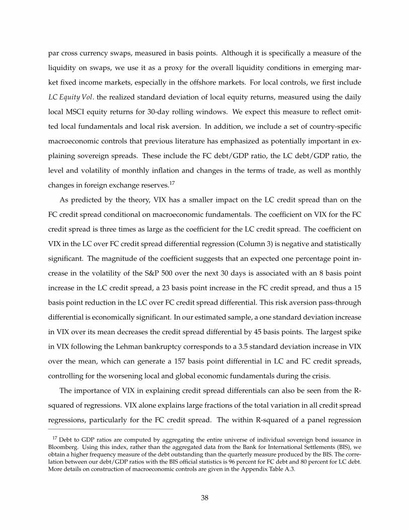
par cross currency swaps, measured in basis points. Although it is specifically a measure of the

liquidity on swaps, we use it as a proxy for the overall liquidity conditions in emerging mar-

ket fixed income markets, especially in the offshore markets. For local controls, we first include

LC Equity Vol. the realized standard deviation of local equity returns, measured using the daily

local MSCI equity returns for 30-day rolling windows. We expect this measure to reflect omit-

ted local fundamentals and local risk aversion. In addition, we include a set of country-specific

macroeconomic controls that previous literature has emphasized as potentially important in ex-

plaining sovereign spreads. These include the FC debt/GDP ratio, the LC debt/GDP ratio, the

level and volatility of monthly inflation and changes in the terms of trade, as well as monthly

changes in foreign exchange reserves.17

As predicted by the theory, VIX has a smaller impact on the LC credit spread than on the

FC credit spread conditional on macroeconomic fundamentals. The coefficient on VIX for the FC

credit spread is three times as large as the coefficient for the LC credit spread. The coefficient on

VIX in the LC over FC credit spread differential regression (Column 3) is negative and statistically

significant. The magnitude of the coefficient suggests that an expected one percentage point in-

crease in the volatility of the S&P 500 over the next 30 days is associated with an 8 basis point

increase in the LC credit spread, a 23 basis point increase in the FC credit spread, and thus a 15

basis point reduction in the LC over FC credit spread differential. This risk aversion pass-through

differential is economically significant. In our estimated sample, a one standard deviation increase

in VIX over its mean decreases the credit spread differential by 45 basis points. The largest spike

in VIX following the Lehman bankruptcy corresponds to a 3.5 standard deviation increase in VIX

over the mean, which can generate a 157 basis point differential in LC and FC credit spreads,

controlling for the worsening local and global economic fundamentals during the crisis.

The importance of VIX in explaining credit spread differentials can also be seen from the R-

squared of regressions. VIX alone explains large fractions of the total variation in all credit spread

regressions, particularly for the FC credit spread. The within R-squared of a panel regression

17 Debt to GDP ratios are computed by aggregating the entire universe of individual sovereign bond issuance inBloomberg. Using this index, rather than the aggregated data from the Bank for International Settlements (BIS), weobtain a higher frequency measure of the debt outstanding than the quarterly measure produced by the BIS. The corre-lation between our debt/GDP ratios with the BIS official statistics is 96 percent for FC debt and 80 percent for LC debt.More details on construction of macroeconomic controls are given in the Appendix Table A.3.

38

with VIX as the only regressor is equal to 24.7 for the LC credit spread, 58.5 percent for the FC

credit spread, and 25.6 percent for the credit spread differential. Conditional on macroeconomic

fundamentals, VIX increases the R-squared of the regression from 27.1 to 30.1 percent for the

LC credit spread, from 62.2 to 72.8 percent for the FC credit spread and from 36.4 percent to

42.6 percent for the differential. Therefore, VIX alone accounts for 60 percent of total explained

variations in the credit spread differential. After controlling for fundamentals, VIX accounts for an

increase equal to 15 percent of total explained variations in explanatory power of the benchmark

regression.

Conditional on our host of controls, swap liquidity does not significantly affect the LC credit

spread. Although the bid-ask spread of the swap significantly increases with the swap rate, it is

also associated with a similar increase in the nominal LC over US spread. On the other hand, the

FC credit spread significantly increases with the bid-ask spread, despite the fact that no swaps

are used in the construction of the measure. This supports our use of the bid-ask spread on the

swap as a general measure of liquidity as well as a direct measure of swap liquidity. Furthermore,

we find that worsening global macroeconomic conditions, higher local equity volatility, higher FC

debt/GDP and higher inflation volatility all significantly increase the FC credit spread, but have

either insignificant or smaller impacts on the LC credit spread.

39

Table 1.6: Regression of 5-Year Credit Spreads on VIX, 2005m1-2011m12. The dependent variables areas follows: (1) sSLC/US, swapped LC over U.S. Treasury spread; (2) sFC/US, FC over U.S. Trea-sury spread; (3) sSLC/FC, swapped LC over FC spread; (4) sLC/US, unhedged LC over US Trea-sury spread; (5) CCS, 5-year zero-coupon cross-currency swap rate. The independent variablesare: VIX, monthly standard deviation of implied volatility on S&P index options (conventionalquote/

√12); CFNAI, Chicago Fed National Activity Index; baCCS/s, one half of bid-ask spread

on 5-year par CCS in basis points; LC Equity Vol., realized standard deviation of daily local MSCIequity returns computed using a moving window of 30 days; ∆IP, monthly percentage change incountry-specific industrial production index; FC Debt/GDP and LC Debt/GDP, monthly LC and FCdebt to GDP ratios aggregating from the entire universe of Bloomberg sovereign bonds outstand-ing; ∆CPI, monthly percentage change in consumer price index; Std(∆CPI), standard deviationof ∆CPI for the past 12 months; ∆ToT, monthly percentage change in terms of trade; Std(∆ToT),standard deviation of ∆ToT for the past 12 months; and ∆Reserve, monthly percentage change inFX reserves. All regressions are run at monthly frequency with country fixed effects using Newey-West standard errors with 12-month lags clustered by month following Driscoll and Kraay (1998)*** p<0.01, ** p<0.05, * p<0.1.

(1) (2) (3) (4) (5)sSLC/US sFC/US sSLC/FC sLC/US ccs

VIX 0.088*** 0.23*** -0.15*** 0.16*** 0.070**(0.029) (0.019) (0.025) (0.043) (0.031)

CFNAI -0.017 -0.16*** 0.15 -0.15 -0.13(0.082) (0.040) (0.094) (0.14) (0.13)

baCCS 0.0037 0.025*** -0.021*** 0.024*** 0.020***(0.0049) (0.0025) (0.0056) (0.0092) (0.0058)

LC Equity Vol. 0.12 0.19** -0.065 0.19 0.071(0.075) (0.082) (0.054) (0.17) (0.12)

∆IP -0.10 -0.076* -0.027 0.084 0.19*(0.066) (0.040) (0.073) (0.11) (0.096)

Other Controls

FC Debt/GDP -0.026 0.12*** -0.15*** 0.0096 0.035LC Debt/GDP -0.024 0.011 -0.035*** -0.052*** -0.028***∆CPI 0.10* 0.033 0.068* 0.32*** 0.21***Std(∆CPI) 0.39** 0.50*** -0.10 1.09*** 0.69***∆ToT -0.0086 0.0077 -0.016** 0.011 0.019***Std(∆ToT) 0.024 0.021 0.0032 0.27*** 0.25***∆Reserve -0.0013 -0.011 0.010 -0.029** -0.028**Observations 762 762 762 762 762Within R-Squared

Full model 0.301 0.728 0.426 0.442 0.308Without VIX 0.271 0.622 0.364 0.415 0.299With VIX only 0.247 0.585 0.256 0.266 0.111

40

1.5.2 Cross-Country Variation

We now relax the assumption that the pass-through of global risk-aversion into FC debt, δFC,

is the same across all countries. The theory predicts that the ratio of swapped LC to FC pass-

thorough δSLCi /δFC

i increases in ρir. To test this prediction, we obtain estimates of δSLC

i and δFCi from

the coefficients on the interaction terms between country dummies and VIX in the regression:

sji,t = α

j1,i + ∑

iδ

ji Ciγt + λczi

t + λwzwt +

jit, (1.3)

where the country dummy Ci = 1 for country i. Columns 1 and 2 of Table 1.7 report the coefficient

estimates for δSLCi and δFC

i . For our model to find empirical support, we would expect countries

with a higher ratio δSLCi /δFC

i to have a higher return correlation. As demonstrated by comparing

Column 3, where we compute this ratio country by country, and Column 4, where we present the

return correlations, this is precisely what we find, with the correlation between the two columns

at a remarkable 84 percent. Differential sensitivities to VIX explain the bulk of the cross-sectional

variations in excess return correlations. We present this result visually in Figure 1.9, showing once

again that the strong positive relationship between the pass-through of risk aversion into the LC

credit spread relative to the FC credit spread and the return correlation between the two assets.

41

Brazil

Colombia

Hungary

Indonesia

Israel

Mexico

Peru

Philippines

PolandTurkey

0.3

.6.9

1.2

1.5

Ratio

of LC

ove

r F

C r

isk

ave

rsio

n p

ass

−th

oro

ugh

−.2 0 .2 .4 .6 .8 1Return Correlation

Figure 1.9: Differential Risk Aversion Pass-Though and Return Correlation. This figure plots the ratio ofglobal risk aversion pass-through into LC credit spreads over the pass-through into FC creditspreads on the y-axis (Column 3 in Table 1.7) and correlation between swapped LC and FCquarterly holding period returns over U.S. Treasury bill rates on the x-axis (Column 4 in Table1.7). The ratio of pass-through is computed based on Columns 1 and 2 in Table 1.7. The fullregression specification is given by Equation 1.3.

42

Table 1.7: Impact of VIX on Credit Spreads by Country. This table reports results of cross-country vari-ations in the impact of VIX on credit spreads. Columns (1) and (2) report coefficients on VIXinteracting with country dummies in credit spread regressions with macroeconomic controls, asspecified by Equation 1.3. Column (1) reports the pass-through of VIX into LC credit spreads andColumn (2) reports the pass-through of VIX into FC credit spreads. All controls are the same asin regression Table 1.6. All regressions are run at monthly frequency with country fixed effectsusing Newey-West standard errors with 12-month lags clustered by month following Driscoll andKraay (1998) *** p<0.01, ** p<0.05, * p<0.1. Column (3) computes the ratios of coefficients inColumn (1) over Column (2) and Column (4) reports the correlation between swapped LC andFC quarterly excess returns over the U.S. T-bill rates. A scatter plot of columns (3) against (4) isshown in Figure 1.9.

(1) (2) (3) (4)δSLC δFC δSLC/δFC ρi

r

Brazil 0.19*** 0.14*** 1.33 0.73(0.044) (0.025)

Colombia 0.046 0.24*** 0.19 0.32(0.028) (0.020)

Hungary 0.31*** 0.35*** 0.88 0.56(0.055) (0.059)

Indonesia -0.010 0.39*** -0.03 -0.13(0.045) (0.076)

Israel 0.051 0.064* 0.79 0.91(0.045) (0.034)

Mexico 0.066* 0.19*** 0.35 0.39(0.039) (0.022)

Peru 0.043 0.23*** 0.19 0.16(0.035) (0.037)

Philippines 0.016 0.24*** 0.07 0.21(0.045) (0.043)

Poland 0.11*** 0.19*** 0.59 0.62(0.031) (0.036)

Turkey 0.21*** 0.36*** 0.57 0.48(0.055) (0.033)

All Macro Controls Yes Yes Correlation (3) and (4)Observations 762 762 0.84

R-squared 0.404 0.782

43

1.5.3 Excess Returns Predictability

We now present evidence on how differential risk premia affect the time series properties of

credit spreads. Since VIX has a contemporaneous positive impact on credit spreads through the

risk premium channel, high levels of VIX are associated with high risk premia, and hence high ex-

cess returns over U.S. Treasury bonds. Since VIX has a differential contemporaneous pass-through

into LC and FC credit spreads, we should also expect VIX to have differential predictive power

for LC and FC excess returns. Consistent with the prediction, we find that high VIX predicts

higher FC excess returns than swapped LC excess returns, and thus negative swapped LC over

FC excess returns. The negative predictive power of VIX for swapped LC over FC excess returns

naturally gives rise to an investment strategy. When global risk aversion is high, an arbitrageur

can long FC bonds and short swapped LC bonds. Since FC spreads are much more sensitive to the

global risk aversion shocks than swapped LC, high risk aversion predicts positive excess returns

on this strategy, which compensates for the risk that the arbitrageur takes. On the other hand,

global macroeconomic fundamentals marginally forecast persistence, rather than mean reversion

in swapped LC over FC excess returns once VIX is controlled. Therefore, it is unlikely that the

predictive power of VIX is due to its correlation with unobserved macroeconomic fundamentals.

In the first panel of Table 1.8, we examine the forecasting power of these variables for annual-

ized excess returns of swapped LC bonds over U.S. Treasury bonds for a quarterly holding period.

In the first regression, we see that high levels of VIX forecast excess returns at the quarterly hori-

zon with an R2 of 4.2%. We next run a second univariate forecasting regression and find that

CFNAI, our measure of local fundamentals, has similar forecasting power as VIX for swapped LC

excess returns. When we run a bivariate forecasting regression including both VIX and CFNAI in

the third row, both lose significance and the increase in forecasting power is marginal compared

to including VIX alone. Including the spread on the cross currency swap rate baCCS/2 and the

volatility on the local equity indices LC Vol have little effect, but including industrial production

growth ∆IP leads to a significant increase in forecasting power. Higher industrial production

growth forecasts lower excess returns on swapped LC bonds.

In the second panel of Table 1.8, we repeat this forecasting exercise for excess returns on FC

bonds over U.S. Treasury bonds. In the first row, we see that VIX alone has an R2 of 10.1% and

44

the coefficient on VIX is more than double the coefficient on VIX in the univariate regressions for

excess returns on swapped LC bonds, and the R2 is more than doubled as well. In the second

regression, we once again remove VIX to examine the forecasting power of CFNAI alone and

find that, in contrast to the results in the first panel, the R2 is only one quarter the value it is in

the univariate forecast using VIX. In the third row, we see that a forecasting regression with both

VIX and the CNFAI has an R2 less than one percentage point higher than for VIX alone. The

key finding is that conditional on VIX, the global fundamental does not forecast mean reversion

in returns. The magnitude of the coefficient on VIX actually increases by 45 basis points after

controlling for CFNAI, once again in sharp contrast to the forecasting results for swapped LC

excess returns. In the fourth row, we add our liquidity measure to these two variables and find

that the forecasting power of the regression is increased significantly to 15.5%. After adding the

full set of local controls, the coefficient on VIX is significantly positive at 2.82.

Finally, in the third panel, we examine how these variables forecast excess returns of swapped

LC bonds over FC bonds. In the first row, we see that higher levels of VIX forecast a negative

excess return of swapped LC over FC debt, as would be expected since we found in the first two

panels that elevated levels of VIX forecast much higher FC returns than swapped LC returns.

Looking at all 6 forecasting regressions in the third panel, we see that the forecasting strength of

VIX is sharpened as we add in our measures for global fundamentals, global liquidity, local market

conditions, and miscellaneous controls. Because VIX covaries strongly with global fundamentals

and global fundamentals marginally forecast return persistence, the predictive power of VIX is

increased when we condition on fundamentals. Conditional on fundamentals, a one standard

deviation increase in VIX over its mean forecasts negative 6.3 percent annualized excess returns

of swapped LC over FC bonds.

45

Table 1.8: Forecasting Quarterly Holding-Period Excess Returns, 2005m1-2011m12. This table reports an-nualized quarterly return forecasting results for srxLC/US

t+3 , swapped LC over U.S. excess returns,rxFC/US

t+3 , FC over US excess returns, and srxLC/FCt+3 , swapped LC over FC excess returns. See Ta-

ble 1.6 for definition of predictive variables. All regressions are run at monthly frequency withcountry fixed effects using Newey-West standard errors with 12-month lags clustered by monthfollowing Driscoll and Kraay (1998) *** p<0.01, ** p<0.05, * p<0.1.

VIX CFNAI baCCS/2 LC Vol ∆IP Other Controls R2

(1) 0.92** No 0.042(0.41)

(2) -2.95** No 0.037(1.24)

(3) 0.620 -1.460 No 0.047(0.43) (1.53)

srxLC/USt+3 (4) 0.600 -1.370 0.0320 No 0.048

(0.45) (1.52) (0.046)(5) 0.440 0.210 0.0180 1.010 -3.77*** No 0.078

(0.48) (1.25) (0.047) (0.98) (1.24)(6) 0.710 -0.0770 -0.0210 0.300 -3.45** Yes 0.106

(0.54) (0.98) (0.045) (1.08) (1.50)(1) 1.95*** No 0.101

(0.66)(2) -3.330 No 0.025

(2.26)(3) 2.49** 2.620 No 0.109

(1.07) (3.60)rxFC/US

t+3 (4) 2.21** 3.550 0.33*** No 0.155(1.01) (3.78) (0.098)

(5) 2.08* 5.100 0.32*** 0.820 -3.69** No 0.170(1.11) (3.80) (0.090) (1.32) (1.53)

(6) 2.82** 4.790 0.28*** 0.0240 -2.530 Yes 0.212(1.36) (3.44) (0.065) (1.43) (1.69)

(1) -1.03*** No 0.028(0.29)

(2) 0.380 No 0.000(1.32)

(3) -1.87*** -4.09* No 0.047(0.66) (2.35)

srxLC/FCt+3 (4) -1.61*** -4.93* -0.30*** No 0.085

(0.60) (2.60) (0.11)(5) -1.64** -4.89* -0.30*** 0.190 -0.0790 No 0.085

(0.67) (2.75) (0.11) (1.05) (0.99)(6) -2.12** -4.87* -0.30*** 0.270 -0.910 Yes 0.111

(0.86) (2.68) (0.089) (1.05) (0.80)

46

1.6 Conclusion

The last decade has seen a remarkable change in emerging market government finance. No

longer do major emerging markets have to borrow in external markets in FC to borrow from

global investors. Instead, global investors are increasingly willing to lend to emerging market

governments by investing in LC debt issued in domestic markets. Despite these major changes,

the academic literature on sovereign risk still remains focused on emerging market debt crises

involving FC debt issued abroad. In this paper, we tried to understand the impact of these changes

by jointly examining the sovereign risk on LC and FC debt. To do so, we introduce a new measure

of LC sovereign risk, the LC credit spread, defined as the difference between LC bond yield and

the LC risk-free rate implied from the swap market.

This new measure delivers several key findings. First, emerging market LC bonds promise to

pay a significant positive spread over the risk-free rate, direct evidence for the failure of long-term

covered interest rate parity for government bond yields between emerging markets and the United

States. Second, LC debt has lower credit spreads than FC debt issued by the same sovereign at

the same tenor. The LC over FC credit spread differential becomes even more negative during

the peak of the crisis. Third, FC credit spreads are very integrated across countries and more

responsive to global risk factors, but LC credit spreads are much less so. From an offshore in-

vestor’s perspective, the commonly perceived systematic risk on LC debt mainly comes from the

currency risk. Once the currency risk is hedged, LC bonds are safer than FC bonds in terms of the

correlations between asset returns and global risk factors.

We rationalize these new empirical findings using a model allowing for partial integration

between domestic and external debt markets. The model features local investors with preferred

habitats in the LC debt and risky credit arbitrage between the domestic and external markets.

The equilibrium LC credit spread is a weighted average of credit valuation of local clienteles and

offshore investors. Consistent with the model’s prediction, we find that differential exposure to

global risk aversion explains a significant portion of the cross-country and time series variations

in credit spread differentials, conditional on a host of macroeconomic variables. The differential

sensitivities of LC and FC credit spreads to global risk aversion shocks sheds light on the degree

of market integration between domestic and external debt markets.

47

While our reduced form model captures many of the new stylized facts that we document,

we have abstracted from how the sovereign decides whether to issue LC or FC debt. Integrating

our empirical findings using price data into sovereign issuance patterns using bond supply and

ownership data is part of ongoing research.

48

2. THE END OF“ORIGINAL SIN”: NOMINAL BOND RISK IN EMERGING

MARKETS1

2.1 Introduction

Today, emerging markets rarely issue local currency (LC) debt in international markets but

they are borrow from foreign lenders in their own currency. This apparent contradiction comes

from the fact that foreign investors are increasingly investing directly LC sovereign bonds issued

in domestic markets under domestic law. While this may seem to be an insignificant develop-

ment, we argue that it demonstrates the end of a major issue in international economics: “Original

Sin.” In an important and influential paper, Eichengreen and Hausmann (1999) demonstrated that

emerging markets were particular vulnerable to financial crises because they had all of their exter-

nal liabilities denominated in foreign currency (FC). A large literature followed, emphasizing that

a country’s inability to borrow abroad in their own currency at long tenors, “Original Sin” was a

major source of macroeconomic fragility in emerging markets.

In this paper, we demonstrate just how dramatically this situation has changed over the last

decade and show that local currency now constitutes a large and growing portion of emerging

market sovereign external borrowing. However, countries did not overcome Original Sin by issu-

ing LC debt in international markets. Rather, foreign investors began lending to emerging markets

by purchasing bonds in domestic markets, even though this leaves them exposed to capital control

risk, custodial risk, and other risks in addition to the nominal risks of inflation and exchange rate

depreciation. Using a new compiled dataset on foreign participation in domestic sovereign bond

markets, we show that since the mid-2000s, foreign ownership has been growing rapidly and now

stands at over 20 percent of total domestic debt outstanding for many countries, and significantly

higher for several emerging markets. Using more refined ownership data for Brazil, Poland, Peru

1 Joint with Jesse Schreger, Harvard University

49

and Mexico, we show that foreigners are particularly interested in holding nominal fixed rate

bonds, even when inflation-linked and floating-rate bonds are available. For many emerging mar-

kets, LC debt not only provides the majority of government finance, but also provides the majority

of financing from foreign investors.

Du and Schreger (2013) study the behavior of the credit component of LC sovereign bonds by

hedging away nominal interest rate risk using currency swaps, and contrast it with dollar credit

spread on the external debt issued by the same sovereign. In this paper, we directly study the

risk of LC nominal bonds without of hedging away the duration risk. We focus on the excess

holding period returns of LC bonds over LC short rates for local investors. From dollar investors’

perspective, this approximates the dollar excess return on LC bonds over the dollar short rate after

hedging away the currency risk of the holding period. Using the systematic exposure of bond

duration risk with local and global equity risk factors, we address the following three questions.

First, how are nominal bond risks different across countries? Second, why are nominal bond risks

different across countries? And third, what is the implication of differential nominal bond risk on

sovereign debt portfolio consisting of local and FC debt?

Examining a sample of 11 developed markets and 20 emerging markets from 2005 to 2012, we

find that while emerging market equity returns are far more correlated with US equity returns

than emerging market bond returns are with US Treasury returns. The lack of synchronization in

nominal bond returns between emerging markets and the U.S. reflects large cross-country vari-

ations in risk of nominal bonds. We define the risk of nominal bonds as the CAPM betas of the

bond excess returns on local and global equity excess returns. We show that nominal bonds in

G10 currencies all have negative betas with local equity and S&P excess returns. In the sample of

emerging markets, local bond betas with local equities exhibit large cross-country heterogeneity,

ranging from -0.14 for Hong Kong to 0.3 for Indonesia.

We then explain the cross-sectional distribution of bond betas in terms of cross country differ-

ences in the conduct of monetary policy. The negative betas of G10 currency bonds for the sample

period is consistent with the finding that in developed countries, government bonds have become

a good hedge for equity investors over the past decade.2 Under countercyclical monetary policy

2 Eurozone countries experiencing sovereign debt crises are obvious exceptions.

50

and procyclical inflation rates, negative macroeconomic shocks lower inflation expectation and

increase expected future real cash flows, giving rise to positive returns on nominal bonds. For

emerging markets, one of the main benefits of being able to borrow using nominal fixed rate LC

debt is that it provides more state contingency compared with FC borrowing. During the bad

states of the world, the government has the option to resort to inflation to reduce the real burden

of the debt. In anticipation of inflationary policy during downturn, nominal bonds may carry

positive inflation risk premium. We document a large degree of heterogeneity across our sample

countries in the degree to which LC debt acts a hedge for the return on the market portfolio.

The risk profile of LC nominal bonds have significant implications on a country’s sovereign

debt portfolios and external default risk. The cross-sectional variation in bond betas are strongly

correlated with the primary external sovereign default risk measure, the sovereign credit default

swap (CDS) spreads. Countries with higher bond betas also have high CDS spreads, with the

cross-sectional correlation at 91 percent. Furthermore, countries with negative or low bond betas

almost exclusively borrow in local currencies, whereas countries with high bond betas rely more

on FC financing.

We test the hypothesis that the risk differential can be explained by the cyclicality of monetary

policy. Using professional forecast data, we compute the sensitivity of revisions to output forecasts

with respect to revisions to inflation forecasts as a proxy for investors’ ex-ante expectation of the

cyclicality of inflation. We show countries with higher expected inflation procyclicality tend to

have lower bond betas. In addition, we show that cross-sectional and time series variation in the

perceived inflation procyclicality are highly correlated with the development of LC nominal bond

markets. The expansion of nominal debt markets coincided over the past decade with a sharp

reduction in the counter-cyclicality of inflation rates.

To better understand these observed empirical patterns, we develop a simple general equilib-

rium model where the sovereign decides whether to borrow in LC or FC debt. We show that when

the government is unable to commit to repayment or to state-contingent inflation rules, countries

with higher external financing needs tend to have lower fractions of debt financed in LC, higher

default risk, higher inflation levels and inflation risk premia. In an extension with a decision be-

tween financing borrowing domestically or externally, we show that the option to borrow from

51

domestic markets can alleviate the time-consistency problem due to external borrowing and shift

the currency composition of the external sovereign debt portfolio toward LC debt.

2.2 Related Literature

In addition to building on recent empirical work on LC domestic debt (Du and Schreger, 2013

and Burger, Warnock, and Warnock, 2012), our paper directly addresses the large literature on

“Original Sin”. This large literature, beginning with Eichengreen and Hausmann (1999), points

to the absense of international issuances of long-term fixed coupon LC debt as a missing market.

Eichengreen and Hausmann (1999) discuss a number or reasons for the absence of this market,

briefly discussing our favored explanation, saying “If a country was able to borrow abroad in its

own currency, it would stand to benefit by depreciating that currency and thus eroding the real

value of its external debts. In anticipation of this, foreigners are unwilling to lend in a denomina-

tion that the borrower can manipulate unless they are compensated to an extent that only those

borrowers planning to devalue are prepared to pay.” We build on this line of thinking, arguing

that the strength of the temptation to inflate away debt ex post will factor into a government’s

optimal choice of the currency composition ex ante. By looking at this issue in general equilib-

rium we show that if a country’s external financing needs are large, a government might shift its

currency composition of debt towards FC debt, eschewing LC debt at higher interest rates.

By collecting a new dataset on foreign holdings of domestic debt, our work fills in an impor-

tant gap in the empirical research on the currency composition of sovereign debt, such as Eichen-

green, Hausmann, and Panizza (2005a). Hausmann and Panizza (2011) also examine foreign par-

ticipation in emerging market LC debt markets using surveys of US investors from 2003-2007.

While these authors presented compelling evidence that emerging markets issued little to no debt

abroad, Reinhart and Rogoff (2008, 2011) present evidence that domestic debt was always an im-

portant part of emerging market government finance. We view our present work as integrating

these two lines of inquiry: while very little debt issued under foreign law and in international mar-

kets is in LC, as demonstrated in the Original Sin literature, we argue that foreign investment in

LC bonds issued in domestic markets under domestic law takes the place of the “missing market”

discussed in Eichengreen and Hausmann (1999).

52

Our paper builds on recent work by Campbell, Sunderam, and Viceira (2013) demonstrating

that the covariance between US Treasury bond returns and stock returns has changed dramatically

the past few decades. Campbell, Sunderam, and Viceira (2013) show that since the mid-1990s

the covariance has become negative, meaning that US nominal bonds are now a hedge for the

domestic equity market. We build on their work by examining the cross-country heterogeneity

in bond/stock covariances in emerging markets and argue that this heterogeneity helps under-

stand the different risk premia embedded in LC debt and the different currency composition of

sovereign portfolios.

Our theoretical framework builds on the optimal debt management literature, in particular the

time consistency argument presented in Bohn (1988, 1991). Bohn (1988) demonstrates that when

taxation is costly, a welfare maximizing government will issue nominal debt to help smooth the

tax burden over time. However, issuing nominal debt worsens the time inconsistency problem in

monetary policy, as existing nominal debt can effectively be treated as an inelastic tax base. Bohn

(1991) illustrates how this time inconsistency problem is worsened in the open economy, as in

addition to tax-smoothing motives, if nominal debt is held by foreigners and the government is

only concerned with domestic welfare, policymakers will be tempted to use surprise inflation to

achieve a real wealth transfer from foreign lenders to domestic residents. Niemann, Pichler, and

Sorger (Forthcoming) quantifies the time inconsistency induced by nominal debt in the closed

economy and demonstrates how the time consistency problem in nominal debt can explain infla-

tion persistence. Our paper builds on this line of research by examining the question in an open

economy and introducing sovereign default. Whereas in Bohn’s work, the government might

find it optimal to overcome the time inconsistency problem by issuing real debt, these papers did

not address the possibility that the government lacked the ability to commit to repaying this real

debt. By introducing a government debt denomination choice along with sovereign default, our

paper addresses how governments can use a mix of debt denomination to try to alleviate the time

inconsistency problem inherent in both types of sovereign borrowing.

Our paper also contributes to the large literature on sovereign default, beginning with Eaton

and Gersovitz (1981), and the quantitative models of sovereign default following Aguiar and

Gopinath (2006). Our paper is most similar to Aguiar, Amador, Farhi, and Gopinath (2013), where

the authors also consider defaultable nominal debt and how inflation commitment affects the

53

probability of outright default. Our paper differs from Aguiar, Amador, Farhi, and Gopinath

(2013) in a few important ways: first, we examine strategic default rather than rollover crises,

second, we introduce portfolio choice so that only an (endogenous) fraction of the debt is de-

faultable, and third, we introduce domestic creditors as an additional source of financing. Our

paper is also similar to Arellano and Ramanarayanan (2012) by introducing government portfolio

choice into a quantitative model of sovereign default. While these two papers consider short-term

and long-term debt, and we consider the currency composition, both papers are focused on the

optimal portfolio of defaultable sovereign debt to best hedge against shocks hitting the economy.

Finally, our paper is closely related to Broner, Martin, and Ventura (2010) and Broner, Erce, Martin,

and Ventura (2013) on the interaction between domestic and external creditors in the secondary

markets.

2.3 The End of “Original Sin”

We construct a new dataset of ownership of domestic debt in 11 emerging markets from indi-

vidual central banks, finance ministries, and the Asian Development Bank. Our data for Peru and

Poland contain monthly data on the ownership structure at the individual bond level, with data

for both countries coming from the respective Ministries of Finance. For Colombia and Brazil, our

dataset contains monthly ownership data at the level of broader security classes (fixed coupon,

inflation-indexed, floating rate, or foreign exchange linked debt). We have daily data at a similar

level of disaggregation for Mexico from the central bank.3 Data for Hungary and Turkey are also

from the national central banks but are not available at similar levels of disaggregation. Owner-

ship data for Indonesia, South Korea, Thailand, Japan, Malaysia comes from AsianBondsOnline,

an online data source produced by the Asian Development Bank. For these countries only aggre-

gate LC debt ownership at a quarterly frequency is available. Finally, for the US, UK and European

countries, we use the dataset constructed by Merler and Pisani-Ferry (2012).

Contrary to the common belief that emerging markets cannot borrow in their own currency

at fixed nominal rates, Figure 2.1 shows that the share of LC debt owned by foreigners increased

3 The Mexican and Polish data is available on the government websites. We digitized monthly reports (available asPDFs) online to construct our time series for Peru and Colombia. We received the Brazilian data from the central bank.

54

from 9 percent in 2005 to 23 percent in 2011 in the sample emerging markets, now higher than the

share in Japan, comparable with the share in the US and the UK, albeit lower than the share in the

euro area. Figure 2.2 gives the time series of foreign ownership of domestic LC debt during the

past decade. Foreigners started buying into LC bond markets in the mid-2000s except for Hungary

and Poland where foreign ownership took place earlier. During the peak of the Global Financial

Crisis in 2008-09, foreigners significantly reduced their holdings. The trend rapid growth resumed

shortly after the crisis peak.

Figure 2.1: Foreign Ownership of Government Debt in Emerging and Developed Markets. This figuredisplays shares of domestic government debt owned by foreigners in emerging markets anddeveloped countries. Data sources are described in Section 2.3.

In addition, for countries with ownership data by security class (Mexico, Brazil, Peru and

Poland), we show in Figure 2.3 that foreigners are particularly interested in holding nominal

bonds, even though inflation-linked and floating-rate bonds are available. Peru, a country that

experienced hyperinflation as recently as 1990, now finances more than 60 percent of its LC debt

from foreigners in nominal fixed rate instruments. Figure 2.4 displays this remarkable change in

Peru. The left panel plots the ownership structure of all LC bonds outstanding in February, 2004.

The majority of LC fixed coupon bonds had under three years of remaining maturity and all were

held locally. This picture has completely changed by December, 2012, where most of the debt has

a remaining maturity of more than 10 years and the majority is now foreign-owned.

Putting these new stylized facts together, we can see that foreign investors have a growing

appetite for nominal risk in emerging markets. LC debt is an increasingly important component

55

0.2

.4.6

Fra

ctio

n o

f to

tal

2003q1 2005q3 2008q1 2010q3 2013q1quarter

Hungary Mexico Turkey

Poland Colombia Indonesia

Malaysia South Korea Thailand

Brazil Peru

Foreign ownership of domestic LC debt

Figure 2.2: Time Series of Foreign Ownership of Government Debt in Emerging Markets. This figureplots time series of fraction of LC debt owned by foreigners for sample emerging markets. Datasources are described in Section 2.3.

of external debt. While the “Original Sin” hypothesis seemingly holds in the very strict sense that

most emerging market debt issued in international markets is still in FC, it is mostly likely due to

sovereigns’ unwillingness rather than inability to tap international markets in LC. As discussed in

Du and Schreger (2013), a few emerging markets, such as Brazil, Colombia and Philippines, have

issued LC denominated bonds in the international market. These offshore bonds are traded at

significantly lower yields compared with onshore bonds. From a foreign investor’s perspective,

offshore LC bonds are safer assets because they are governed under international law and free

from capital control risk. If foreign investors are already willing to take onshore nominal risk, it is

difficult to argue why they would not want to hold offshore LC bonds.

56

Figure 2.3: Ownership of Domestic Debt by Security Type in 2012. This figure plots the share of domesticgovernment debt by ownership and security type in the end of 2012. ‘Fixed” denotes fixedor zero coupon nominal bonds; “Inflation” denotes inflation-linked real bonds; and “Floating”denotes floating bonds. Data sources are described in Section 2.3.

57

(a) April 2004

(b) December 2012

Figure 2.4: Ownership Structure of Peruvian Nominal Bonds (millions of nuevo soles). X-axis number ofyears of remaining on maturity on a given bond. “10” indicates bonds with 10-15 years remain-ing maturity, “15” years 15-20 years, and “20” refers to bonds with more than 20 years remiainingmaturity. Vertical axis is millions of nuevo soles. The bars are sums of ownership across bondswithin a given maturity bin. Data sources are described in Section 2.3.

58

2.4 Measuring Nominal Bond Risks

2.4.1 Definition of Nominal Bond Betas

We use Bloomberg fair value (BFV) curves to compute excess holding period return on the

constant maturity 10-year bond yield in emerging markets from 2005 to 2012.4 The BFV curves

are estimated using individual LC sovereign bond prices traded in the secondary markets. Since

sufficient numbers of bonds spanning different maturities are needed for yield curve estimation,

the availability of the BFV curve is a good indicator for the overall development of LC nominal

bond market. Countries such as Argentina, Uruguay and Venezuela only have a handful of fixed-

rate bonds and hence do not have a BFV curve.

Given the log yield on a n-year bond traded at par ycnt = log(Ycnt), the log holding period

return on the bond is given by

rbc,n,t+∆t ≈ Dcnycnt − (Dcn − ∆t)yc,n−1,t+∆t,

where Dcn = 1−(1+Ycnt)−n

1−(1+Ycnt)−1 is the duration of the bond (Campbell, Lo, and Mackinlay, 1997). We

approximate yc,n−∆t,t+∆t by yc,n,t+∆t for the the quarterly holding period (∆t = 0.25). We let y1t

denote the three-month T-bill yield and then the excess return on LC bonds over the short rate is

given by

rxbn,t+∆t = rb

c,n,t+∆t − yt1.

From a dollar investor’s perspective, we can rewrite excess return as

rxbn,t+∆t = [rb

c,n,t+∆t − (yt1 − y∗t1)]− y∗t1.

The dollar investor can hedge away the currency risk of the holding period ∆t by going long a

U.S. T-bill and shorting a LC T-bill with the same market value as the LC bond. By doing so, any

movement in the spot exchange rate of the LC has the same offsetting first-order impact on the

bond position and the local T-bill position and hence cancels out. However, since the cash flow

4 Yield curves for Brazil and Israel are obtained from ANBIMA and the Central Bank of Israel, respectively. SinceTurkey issued 10-year bonds only recently, we use 5-year as benchmark instead for Turkey.

59

is uncertain next period, a dollar investor may under or over hedge depending on the realization

of the bond price and incur a second-order hedging error. Therefore, LC excess returns provide a

first-order approximation of hedged dollar excess return of a LC bond over the U.S. T-bill. Since

currency risk is only hedged away for the holding period, the dollar investor still bears duration

risk of the LC bond.

Alternatively, a dollar investor can choose not to hedge the FX risk. The realized dollar un-

hedged excess return is equal to

rxb,$n,t+∆t = rc,n,t+∆t − (st+∆t − st)− y∗t1 = rxn,t+∆t + [(yt1 − y∗t1)− (st+∆t − st)],

where st denote the spot exchange rate of LC. The unhedged excess return on the LC bond is equal

to equal to LC excess returns plus the realized return on the carry trade strategy of going long in

LC T-bill funded by shorting a dollar T-bill.

We use three measures to compute nominal bond returns. First, we compute the local bond

beta βLi for each country i by regressing LC bond excess return rxb,i

t+∆t on local equity excess returns

rxm,it+∆t:

rxb,it+∆t = αL

i + βLi rxm,i

t+∆t + Lit.

Local betas measure risk exposure of local bond returns on local equity returns. Second, we com-

pute the hedged global beta βGi for each country i by running LC bond excess returns on the S&P

excess returns rxm,SPt+∆ :

rxb,it+∆t = αG

i + βGi rxm,SP

t+∆t + Git .

From a global investor’s perspective, the global beta gives the first-order approximation of the

risk loading of LC bond returns on global equity returns after hedging out currency risk for the

holding period. Finally, if the dollar investor does not hedge the currency risk, in addition to the

bond global beta βGi , the investor takes additional currency exposure β$

i such that

(yit1 − y∗t1)− (si

t+∆t − sit) = α$

i + β$i rxm,SP

t+∆t + $it.

The total exposure of unhedged bond position for the global investor is equal to βGi + β$

i .

60

2.4.2 Cross-country Variations in Nominal Bond Risk

Table 2.1 reports country-level correlation between LC bond excess returns and U.S. Treasury

bond excess returns and between LC equity excess returns and S&P excess returns. Over the

past eight years, equity excess returns in emerging markets are highly correlated with S&P excess

returns with the mean correlation equal to 74 percent. However, LC bond excess returns are much

less correlated with the U.S. Treasury bond excess returns with mean correlation only equal to 36

percent. Among the sample emerging markets, Hong Kong and Singapore have the highest bond

return correlation with the U.S., whereas Russia and Hungary have the lowest. In the developed

world, both equity and bond markets are highly correlated with the U.S. markets. The correlation

between G10 and the U.S. is equal to 82 percent for government bond excess returns and 86 percent

for equity excess returns. Compared with emerging market equities, emerging market LC debt

brings more scope for diversification for global investors.

Figure 2.5 reports local, global and currency betas for developed and emerging markets. The

order of the countries is sorted by their local betas. As we can see, all developed countries have

negative local betas for the sample period. In other words, nominal government bonds offer a

hedge for local equities. Among emerging markets, around half of the sample countries have

negative local betas and the rest have positive local betas. Hong Kong, Thailand and Singapore

have the lowest local betas whereas Colombia, Philippines and Indonesia have the highest local

betas. Since equity markets are highly correlated across countries, the cross-sectional pattern of

global betas follows the the pattern of local betas. The developed countries all have negative global

and local betas of similar magnitude, which reflects high synchronization between equity excess

returns. Among emerging markets, countries also have negative, zero or positive local and global

betas simultaneously. In terms of the magnitude, among the high betas countries, Mexico, Turkey,

Brazil and Colombia have significantly higher local betas than global betas. In these countries,

nominal bonds carry more systematic risk for local investors than for hedged global investors. As

for currency betas, all currencies except for the Yen, Hong Kong dollar and Chinese renminbi have

positive betas with the global equities. For an unhedged dollar investor, after adding up the global

and currency betas, unhedged LC bonds carry significantly positive betas for the majority of the

countries with five exceptions: Switzerland, Japan, Hong Kong, Thailand, Singapore and China.

61

Table 2.1: Equity and Bond Excess Return Correlation with U.S. Markets (2005-2012). The column “Bond”reports correlation between LC bond excess returns over local T-bill rates and U.S. Treasury bondexcess returns over U.S. T-bill rates. The column “Equity” computes LC equity excess returns overlocal T-bill rates and S&P excess returns over U.S. T-bill rates. Correlations are computed at dailyfrequency for the quarterly holding period.

Emerging Markets Bond Equity G10 Currencies Bond EquityBrazil 0.19 0.76 Australia 0.81 0.84Chile 0.59 0.61 Canada 0.91 0.88China 0.32 0.70 Switzerland 0.78 0.85Colombia 0.22 0.54 Denmark 0.84 0.87Czech Republic 0.49 0.76 Germany 0.86 0.89Hong Kong 0.83 0.81 United Kingdom 0.87 0.93Hungary -0.01 0.85 Japan 0.72 0.76Indonesia 0.14 0.73 Norway 0.77 0.85Israel 0.47 0.64 New Zealand 0.75 0.74India 0.44 0.71 Sweden 0.84 0.83Korea 0.54 0.81Mexico 0.49 0.82Malaysia 0.50 0.71Peru 0.15 0.67Philippines 0.21 0.67Poland 0.37 0.85Russia -0.28 0.79Singapore 0.78 0.87South Africa 0.47 0.74Thailand 0.48 0.78Turkey 0.13 0.72EM Mean 0.36 0.74 G10 Mean 0.82 0.86

62

Figu

re2.

5:Lo

cal,

Glo

bala

ndC

urre

ncy

Bet

as(2

005-

2012

).Th

isfig

ure

plot

sLC

bond

beta

sin

stac

ked

colu

mns

.“Lo

calb

eta”

refe

rsto

the

beta

ofLC

bond

exce

ssre

turn

son

loca

lequ

ityex

cess

retu

rns;

“glo

balb

eta”

refe

rsto

the

beta

ofLC

bond

exce

ssre

turn

sw

ithre

spec

tS&

Pex

cess

retu

rns

and

“cur

renc

ybe

ta”

refe

rsto

the

beta

ofcu

rren

cyex

cess

retu

rns

with

resp

ectt

oS&

Pex

cess

retu

rns.

CD

Ssp

read

spl

otth

em

ean

ofob

serv

edso

vere

ign

cred

itde

faul

tsw

apsp

read

sfo

rth

esa

mpl

epe

riod

.All

beta

sar

eco

mpu

ted

usin

gda

ilyda

tafo

rth

equ

arte

rly

hold

ing

peri

od.T

heor

der

ofth

eco

untr

ies

with

inde

velo

ped

and

emer

ging

mar

ketg

roup

sis

sort

edby

the

loca

lbet

a.M

ore

deta

ilsof

defin

ition

sca

nbe

foun

din

Sect

ion

2.4.

1.

63

2.5 What Explains Nominal Bond Risk?

2.5.1 Bond Betas and Sovereign CDS Spreads

The cross-sectional heterogeneity in bond betas is highly correlated with sovereign CDS spreads.

Sovereign CDS contracts offer insurance for investors in the event of sovereign default. For devel-

oped countries, CDS contracts insure against defaults on all Treasury bonds denominated in local

currencies under domestic law. However, in emerging markets, CDS contracts are exclusively

linked to external debt denominated in foreign currencies. Countries such as Singapore and India

do not have any sovereign debt issued in the external mark and hence do not have CDS contracts.

All sovereign CDS contracts are denominated in U.S. dollars and hence the CDS spreads offer an

approximation for the shadow costs of issuing a U.S. dollar debt for different sovereign issuers.5

Despite the large common component driven by global factors in CDS spreads across countries,

the differential perceived sovereign default risk results in differential levels of CDS spreads.

We find that countries with high CDS spreads tend to have high nominal bond betas. This

can be first seen as rising CDS spreads for countries sorted on their local betas in Figure 2.5. To

visualize the relationship more directly, Figure 2.6 displays the scatterplots of local and global

betas of nominal bonds against mean sovereign CDS spreads. The cross-sectional correlation is

remarkably high at 92 percent between local betas and CDS spreads, and 83 percent between

global betas and CDS spreads. Currency betas are only weakly correlated with CDS spreads with

cross-sectional correlation equal to 31 percent.

Since returns on nominal bonds are largely driven by inflation and currency movements, one

hypothesis to explain the correlation between bond betas and CDS is that countries with higher

default risk tend to have higher inflation expectation during the downturns since the country is

more tempted to inflate and default reduce the real debt burden. Whereas for countries with low

default risk, inflation is procyclical and nominal bonds are hedge for equity returns.

5 US sovereign CDS contracts are denominated in euros,

64

BRL

CLPCNY

COP

CZK

HKD

HUF

IDR

ILS

KRW

MXN

MYR

PEN

PHP

PLN

RUB

THB

TRY

ZAR

AUD

CHFDKK

EUR GBP

JPY

NOKNZD

SEK

USD−.2

−.1

0.1

.2.3

Loca

l Beta

0 50 100 150 200 250Mean CDS (bps)

(a) Local Beta versus CDS

BRL

CLP

CNY

COPCZK

HKD

HUF

IDR

ILSKRW

MXN

MYR

PENPHP

PLN

RUB

THB

TRY

ZAR

AUD

CHFDKK

EUR GBP

JPY

NOKNZD

SEKUSD−

.20

.2.4

Glo

bal B

eta

0 50 100 150 200 250Mean CDS (bps)

(b) Global Beta versus CDS

Figure 2.6: Bond Betas and Sovereign CDS Spreads. Figure 2.6(a) plots bond local betas against sovereignCDS spreads. Figure 2.6(b) plots global betas of LC bonds against sovereign CDS spreads.Emerging markets are denoted by solid dots and G10 currency countries are denoted by dia-monds. Betas are defined in Section 2.4.1.

2.5.2 Cyclicality of Inflation Expectation

We hypothesize that the cross-country heterogeneity in LC bond betas might be a result of

the differing cyclicality of monetary policy across our sample countries. If investors believe that

during bad times the country will inflate to reduce the real burden of debt, then they believe

nominal bonds will pay off poorly exactly when market returns are low. If, on the other hand,

deflation (or less inflation) is expected during bad times then LC bonds will act as a hedge (or a less

risky asset) against market returns. We view this as a cross country application of the argument

presented in Campbell, Sunderam, and Viceira (2013).

To measure the expected pro-cyclicality of inflation expectations, we regress the change in the

CPI inflation rate predicted by forecasters on the change in their predicted real GDP growth rate.

In countries where investors believe that monetary policy will be used for fiscal purposes, we

expect forecasters to revise their inflation expectations up when the revise their real GDP growth

rate forecasts down.6

Each month, professional forecasters surveyed by Consensus Economics forecast inflation and

GDP growth for the next calendar year. We use revisions of inflation and GDP forecasts each

month relative to forecasts made three months ago to infer shocks to investors’ expectation of

6 We could do a similar exercise with consumption growth, but this would reduce the sample size.

65

inflation and output. We pool all revisions for 2006 through 2013 (so that the forecasts themselves

were all made post-2005), and run the country by country regressions

∆πt = β0 + βπ,y∆yt + t (2.1)

where t indicates the date the revision is made. Country subscripts are suppressed to keep the

notation more concise. The revisions to inflation forecasts (∆πt) and GDP growth forecasts (∆yt)

are measured as percentage changes of forecasts made at t + h compared to forecasts made at

t.7 The coefficient βπ,y measures the cyclicality of inflation expectation and is the coefficient of

interest. For now, we examine forecast revisions over 3 month periods.

As can be seen in Figure 2.7, at the three month horizon, we find that countries in which LC

debt has a high beta with the local market tend to have a lower βπ,y, meaning that investors expect

less procyclical inflation rates in countries with high bond betas. A similar pattern is observed at

the one and six month horizon. The cross-sectional relationship between bond betas and forecast

betas holds even better when we use unhedged global betas to measure nominal risk.

BRL

CLP

CNY

COP

CZK

HKD

HUF

IDR

ILSKRW

MXN

MYR

PENPHP

PLN

RUB

SGD

THB

TRY

ZAR

AUD

CADCHF

DKKEUR

GBP

JPY

NOK

NZD

SEK

USD

−.5

0.5

1

Fore

cast B

eta

−.2 −.1 0 .1 .2 .3

Local Beta

(a) Forecast Beta versus Local Beta

BRL

CLP

CNY

COP

CZK

HKD

HUF

IDR

ILSKRW

MXN

MYR

PENPHP

PLN

RUB

SGD

THB

TRY

ZAR

AUD

CADCHF

DKKEUR

GBP

JPYNOK

NZD

SEK

USD

−.5

0.5

1F

ore

cast

Beta

−.2 0 .2 .4 .6 .8 1Unhedged Beta

(b) Forecast Beta versus Unhedged Global Beta

Figure 2.7: Forecast Beta and Bond Beta. Figure 2.7(a) plots forecast betas on bond local betas. Figure 2.7(b)plots forecast betas on bond global betas. Emerging markets are denoted by solid dots and G10currency countries are denoted by diamonds. Betas are defined in Section 2.4.1 and Section 2.5.2.

7 Forecasts are originally made in percentages. We rescale the variable x to x ≡

1 +x

100

. Revisions x are defined

x ≡ xt − xt−hxt−h

. Forecasts are generally made monthly, but for some countries in the mid-90s were made in the mid-

1990s.

66

2.6 Implications of Nominal Risk on Sovereign Portfolios

We next use this same measure of inflation cyclicality and examine whether it can explain the

growth of LC bond markets and the cross country heterogeneity. To do so, we use two sources of

aggregate data from the Bank for International Settlements (BIS). The first data source concerns

the percentage of domestic debt that is fixed coupon, floating rate, inflation indexed or linked to

the exchange rate. This data comes from the BIS Working Group questionnaire and is calculated

using all types of domestic debt, not just central government debt. When calculating the fraction

of government debt that is fixed coupon, we assume that the fraction of fixed government debt

is equal to the fraction reported in the survey.8 The second source of data is on the amount of

domestic and external central government debt outstanding comes from the BIS Debt Securities

Statistics. The classification of the data was recently overhauled in early 2013 but we continue to

use the old classification.

In Table 2.2, we regress the fraction of all domestic debt that is in LC fixed rate on a version

of βπ,y. In order to capture the time series component, instead of pooling across the whole period,

we consider 3 month revisions across overlapping two year periods. The variable timing is such

that only forecasts made in the two years prior to the realization of the dependent variable are

used. Because we do not have a strong a priori view on whether this variable should be more

successful in explaining the cross-section or time series, we run these regressions using a variety of

combinations of year and country fixed effects. As can be seen in Table 1, the forecast revision beta

has strong explanatory power for the cross section, with and without year dummy and remains

significant at the 5% level with country FE and country and year FE. We then introduce two other

variables that would be expected to explain the fraction of fixed coupon nominal debt: the level

and volatility of inflation. For the level of inflation, we use the previous year’s annual inflation

and for volatility we use a 24 month rolling average of year-on-year inflation rates. While a higher

inflation rate is associated with a lower level of fixed coupon debt, inflation volatility is not. Our

forecast beta variable remains significant and positive, meaning that increases in the correlation

8 This is a potential source of bias in Table 2.3. We do not have strong evidence that the currency composition ofdomestic corporate and public debt are the same.

67

Table 2.2: Fixed Coupon LC Debt as a Fraction of Domestic Debt. Dependent variable is the share offixed coupon LC debt as a percentage of total LC debt for the BIS Working Group annual survey.Inflation/GDP beta is the coefficient βπ,y in Equation 2.1. Annual Inflation Rate is the year-on-year inflation rate during the past year. Inflation Volatility (24m) is the standard deviation of theyear-on-year inflation rate over the past 24 months.

(1) (2) (3) (4) (5) (6) (7)Inflation/GDP beta 15.81*** 18.32*** 2.796** 2.690** 12.73*** 12.77*** 1.836**

(4.509) (4.779) (1.312) (1.114) (3.161) (3.179) (0.793)Annual Inflation Rate -108.3*** -113.7*** -35.45*

(36.97) (36.54) (19.35)Inflation Volatility (24m) 110.8 160.8

(154.2) (136.5)Constant 66.92*** 67.18*** 20.16*** 15.81*** 74.55*** 73.54*** 13.66

(6.474) (9.943) (0.912) (4.973) (13.91) (14.42) (8.421)Observations 301 301 301 301 247 247 247

R-squared 0.129 0.162 0.868 0.886 0.235 0.236 0.908Year FE No Yes No Yes Yes Yes Yes

Country FE No No Yes Yes No No Yes

between inflation and GDP forecast revisions are associated with higher fractions of debt in fixed

coupon.

In Table 2.3, we examine whether our forecast revision beta can explain the fraction of LC fixed

coupon debt as a fraction of total sovereign debt. We calculate our dependent variable by mul-

tiplying the stock of domestic debt from the BIS Debt Securities Statistics by the fraction of fixed

coupon LC debt in domestic debt, and dividing by total outstanding sovereign debt. The results

are largely similar to the results in Table 2.2, however the results are slightly weaker, perhaps

because the survey data does not refer only to sovereign debt.

68

Table 2.3: Fixed Coupon LC Debt as a Fraction of Total Sovereign Debt. Dependent variable is the shareof fixed coupon LC debt as a percentage of total outstanding sovereign debt. This variable isconstructed by multiplying the fraction of fixed coupon debt as a fraction of domestic debt by theamount of domestic debt outstanding, an dividing by the entire stock of sovereign debt, domesticand external. Inflation/GDP beta is the coefficient βπ,y in Equation 2.1. Annual Inflation Rateis the year-on-year inflation rate during the past year. Inflation Volatility (24m) is the standarddeviation of the year-on-year inflation rate over the past 24 months.

(1) (2) (3) (4) (5) (6) (7)Inflation/GDP beta 11.87*** 13.53*** 2.555* 1.950 9.121*** 9.074*** 1.267

(3.881) (4.200) (1.427) (1.135) (3.056) (3.098) (0.913)Annual Inflation Rate -96.01** -95.08** -21.95

(34.25) (33.09) (16.72)Inflation Volatility (24m) -4.246 21.79**

(10.39) (9.398)Constant 49.66*** 46.94*** 17.33*** 8.755 60.03*** 60.45*** 6.097

(6.705) (10.85) (0.992) (6.361) (13.28) (13.97) (10.29)Observations 243 243 243 243 220 220 220

R-squared 0.102 0.135 0.837 0.866 0.204 0.204 0.894Year FE No Yes No Yes Yes Yes Yes

Country FE No No Yes Yes No No Yes

2.7 General Equilibrium Model of Sovereign Portfolio Choice

2.7.1 Theoretical Framework

In this section, we use a simple two-period general equilibrium model to better understand the

observed empirical patterns that countries with higher default risk on FC debt also have higher

LC nominal bond risk and lower fractions of nominal bonds in their portfolios. We begin by pre-

senting a simple framework where a benevolent government issues debt to finance a project. The

sovereign has the choice of issuing LC or FC debt. The government lacks commitment and optimal

monetary and fiscal policies will not be time consistent in our model. LC debt is vulnerable to ex

post inflation, and both FC and LC debt are vulnerable to ex post default. We solve the model by

backwards induction. Once we solve for the government’s policy functions in the second period,

we can solve for the government’s optimal policy in the first period. The government’s decision

in the first period involves choosing the quantity of bonds to issue in LC or FC.

We examine this problem in stages. First, we solve the second period policy functions when

the government cannot default on its FC debt but it can inflate away its LC debt. Then we solve for

the policy functions when both types of debt can be defaulted on but only LC debt can be inflated

69

away. With these policies functions solved in closed form, we then analyze the government’s first

period problem by focusing on the benchmark case that all borrowing is external.

We include two extensions of the baseline model that we see as important components of fu-

ture research. First, we highlight the role of risk aversion in affecting the currency composition of

sovereign debt. Second, we discuss an extension of the benchmark model to allow the government

to finance domestically to alleviate the time inconsistency due to external borrowing.

2.7.2 Second Period Problem

No Default

Throughout, we assume a benevolent government that maximizes the utility of the represen-

tative agent:

maxD,π

log (c)− θπ, (2.2)

where c is consumption in the final period, π ∈ [0, 1] is the inflation tax, the net inflation rate

divided by one plus the net inflation rate. θ is the utility cost of inflation. D is an indicator for

default, taking the value 1 when the country defaults and 0 otherwise. The government maximizes

utility subject to its budget constraint being satisfied. When the government cannot default on its

debt, the budget constraint is given by

τy = (1 − π)b + b$, (2.3)

where y is output, τ is the tax rate on output, b is LC debt and b$ is FC debt. Individual consump-

tion is given by non-taxed output and domestic holdings of LC debt net of inflation:

c = (1 − τ)y + (1 − π)bh,

where bh is domestic holdings of government debt. Defining foreign holdings of LC debt as

b f ≡ b − bh and imposing that the government’s budget constraint is satisfied, we can rewrite

consumption of the representative agent as

70

c = y − [(1 − π)b f − b$] (2.4)

Because domestic holdings of LC debt are paid for with tax revenue, they have no impact on the

optimal inflation rate chosen in the second period. Instead, the optimal inflation rate will be a

function of output y, foreign holdings of LC debt b f , and foreign holdings of FC debt, b$.

First, we consider the case without default. The government maximizes utility subject to the

budget constraint. There will be three regions, when the inflation tax is equal to zero (as deflation

provides no benefit), when the inflation tax is equal to 1 (hyperinflation) and when the inflation

tax is in the intermediate range. We can characterize the optimal policy function as a piecewise

function

π∗ =

1 i f y < y

1 − y−b$

b f+ 1

θ i f y ≤ y ≤ y

0 i f y > y

(2.5)

where

y = b f

1 +

1θ

+ b$, y =

b f

θ+ b$.

We can understand these cutoffs as follows: if output is above y, the constant marginal cost of

inflation θ exceeds the marginal benefit of increased consumption that such inflation could achieve

through reducing the real debt burden. At when y = y, the marginal cost and benefit are equalized

at an inflation rate of zero. Therefore, for all levels of output greater than y, the marginal cost of

inflation will be strictly greater than the benefit and so the optimal inflation rate is equal to zero.

This threshold is increasing in both LC and FC debt held by foreigners, but it is increasing faster

in holdings of LC debt. This is because the burden of LC debt can be directly inflated away, but

inflation only eases the burden of repaying FC debt by reducing the other repayments that need

to be made. In addition, the threshold is decreasing in the cost of inflation, as a higher cost of

71

inflation reduces the utility gain from inflation and thus enlarges the space where zero inflation is

optimal.

Hyperinflation, on the other hand, is optimal when output is below y. When output is below

this level, the marginal benefit of additional consumption exceeds the marginal cost of inflation

when the inflation tax rate is already at its maximum value, π = 1. This threshold is also increasing

in both LC and FC debt.

For interior realizations of output in between y and y, optimal inflation equates the marginal

utility cost of additional inflation (θ), to the marginal utility of consumption gained by reducing

the real value of debt payments through inflation. Because the marginal cost of inflation is a

constant given our linear cost function, in this interior solution, the representative agent receives

a constant consumption, and utility gains from additional output come through reduced inflation.

Defaultable Debt

Next, we add sovereign default to the framework above. Following Arellano (2008), we adopt

the non-linear default cost function

yd =

y i f y < y

y i f y ≥ y.

This cost function imposes that if a country defaults, all output above a threshold y is seized if

output is initially above this threshold, and no output is lost if the country defaults when output

is below this given threshold. Under this default cost specification, the country would find it

optimal to choose full default on LC and FC debt if default is ever chosen. In addition, the country

will also choose zero inflation upon default. This feature of the model can be relaxed if we allow

partial default or specify a differential default technology with respect to LC and FC debt to induce

selective default. The only distinction between LC and FC debt is that in non-default states, the

country can choose inflation to erode the real value of LC but not FC debt. The linear inflation cost

and the Arellano type default technology together yield closed-form policy functions.

The problem of determining the default regions is one of simply checking whether the utility

the representative agent receives when defaulting, logyd, exceeds the utility she would be re-

72

ceive if the country did not default and followed the optimal inflation policy in Equation 2.5. This,

in turn, depends on the relative cost of inflation and default, as well as the level and currency com-

position of the outstanding debt. Depending on the level of external debt in LC, we summarize

default and inflation policy functions into the following three cases:

1. If b f < θy,

D∗ =

1 i f y < y1

0 i f y ≥ y1

π∗ = 0.

2. If θy ≤ b f ≤ θ exp(θ)y,

D∗ =

1 i f y < y2

0 i f y ≥ y2

π∗ =

0 i f y < y2

1 − y−b$

b f+ 1

θ i f y2 ≤ y ≤ y

0 i f y > y

.

3. If b f > θ exp(θ)y,

D∗ =

1 i f y < y1

0 i f y ≥ y1

π∗ =

0 i f y < y3

1 i f y3 ≤ y < y

1 − y−b$

b f+ 1

θ i f y ≤ y ≤ y

0 i f y > y

.

where the three default thresholds are given by

73

y1 ≡ exp(θ)y + b$

y2 ≡b f

θlog

θyb f

+ b f +

b f

θ+ b$

y3 ≡ y + b f + b$

In the first case, because the country has a very low LC debt stock, the marginal benefit of

inflating debt away is low, and so there are no output realizations for which the country prefers

to inflate fully instead of explicitly default. LC and FC debt become perfect substitutes since the

government never uses the option to inflate away LC debt in equilibrium. In the second case,

when the country has an intermediate level of LC debt and output is above the default threshold

y2, the country would choose zero or positive inflation, but never hyperinflation. In the third case,

the county has high levels of LC debt. When output is above the default threshold y3, there is a

full range of possibility for optimal inflation, ranging from zero to hyperinflation depending on

the output realization and portfolio composition.

Figure 2.8 graphically summarizes government policy in the final period. The graph includes

three surfaces in the LC debt level on the x-axis, FC debt on the y-axis and Output on the z-axis.

The three surfaces, labeled “Zero Inflation”, “Hyperinflation” and “Default”, plot the important

output thresholds. If output is above the Zero Inflation surface, then there will be no default or

inflation for a given amount of LC and FC debt. As would be expected, this surface is increasing

in both FC and LC debt, meaning that the more LC and FC debt a country has, the higher the

output realization needed to make it optimal for the country to choose not to inflate or default.

The second surface is the Hyperinflation surface. If output is below above this surface, and below

the Zero Inflation surface for a given distribution of external LC and FC debt, then the country

will choose an intermediate level of inflation to lower the real burden of debt repayment. The

preferred level of inflation is decreasing in output, so one can think of there being a continuum of

surfaces for inflation rates equal to a constant rate between the Zero Inflation and Hyperinflation

surfaces. Finally, the third and bottom surface is the Default surface. For given LC and FC debt

stocks, if output is between the Hyperinflation and Default surfaces, the country will hyperinflate

74

away its LC debt, but still pays back FC debt. If output is below the threshold defined by the

Default surface, than the country will default on LC and FC debt.

Figure 2.8: Inflation and Default Policy Functions. This figure plots optimal inflation and default thresh-olds for output given any debt portfolio. Details are given in Section 2.7.2.

2.7.3 First Period Problem: External Debt Only

With the final period policy functions fully characterized, we can now examine the first period

problem. We will begin by looking the simplest case, where a government has to finance a fixed

and exogenous amount z by borrowing from foreign lenders and only has to choose the currency

composition of the debt. The government internalizes the fact that it will re-optimize in the second

period according to the policy functions solved for above. Therefore, the general problem of the

government can then be written as

75

maxb f ,b$

E[log(c1)− θπ1]

s.t. z ≤ qb f + q$b$

π1 = π1

y1, b f , b$

D1 = D1

y1, b f , b$

q$ = E[M∗1(1 − D1)]

q = E[M∗1(1 − D1)(1 − π1)]

where M∗1 gives the stochastic discount factor of foreign lenders and π1 (·) and D1 (·) denote the

ex-post policy functions.

Solution to Optimal External Portfolio

We first solve this problem under the assumption of lender risk neutrality (M∗1 = 1) , and a

log-normal distribution for output

y1 = exp

y1

, y ∼ Nµ, σ2 .

Because the optimal choice of LC and FC and debt will generally not have a closed form solution,

we solve the government’s portfolio choice problem numerically for a range of external financing

needs, z. It is worth noting that the lack of commitment to repay the debt gives rise to a natural

borrowing limit. Once LC and FC reach the threshold, higher debt levels reduce revenue raised

due to increasing inflation and default risk.

Because the model is stylized, we try to avoid taking a strong stand on the relative costs of

inflation and default and generally report our solutions for a wide range of inflation costs θ. Our

first result can be found in Figure 2.9, where we show that the optimal fraction of LC debt is

decreasing in the amount that needs to be financed.9 The intuition for this result is that LC debt

is valuable for it’s state contingency but it is costly because the temptation to repudiate the debt

9 When the country is indifferent between LC and FC debt at very low levels of LC debt (Case 1 in Section 2.7.2), weassume that it chooses LC debt.

76

in every state is factored into its price ex ante. Therefore, a higher face value of debt needs to be

issued if lenders expect the debt to always be repudiated. Because inflation is costly, a government

might be able to benefit from the limited commitment available from FC debt. What we see in the

figure is that as more debt needs to be raised, the time inconsistency problem is worsened, and so

the cost begins to outweigh the benefits from state contingency, and so the government chooses to

issue more FC debt.

0 0.05 0.1 0.15 0.2 0.25 0.3 0.35 0.4 0.45 0.50

0.1

0.2

0.3

0.4

0.5

0.6

0.7

0.8

0.9

1

revenue

fraction o

f L

C d

ebt

theta=1.5

theta=1

theta=0.5

theta=0.05

Figure 2.9: Share of LC Debt vs. Amount of Revenue Raised. This figure plots the share of LC debt chosenin the equilibrium portfolios against the total revenue raise for different values of inflation costsθ. Details are given in Section 2.7.3.

In Figure 2.10(a), we see that the government’s optimal portfolio choice interacts in interesting

ways with the optimal inflation rate. While throughout much of the parameter space expected

inflation is increasing for countries with lower inflation credibility θ, we see that for countries with

very low inflation costs and high borrowing needs, mean inflation could actually be lower than

for some countries with higher inflation costs. This is because an optimizing government with

low credibility might respond to their lack of commitment by issuing so much more FC debt that

it becomes less likely inflate away its debt. However, throughout much of the parameter space,

we have the more intuitive result that expected inflation is increasing in the amount of revenue

that needs to be raised as a larger debt burden makes it more tempting to inflate for any level of

output.

77

Figure 2.10(b) plots the mean default rate for the four different levels of inflation cost for given

amounts of borrowing. It is important to remember that at for every amount of revenue raised

the currency composition of the debt stock differs for the different levels of inflation cost. In this

figure, we see that the default probability is increasing in the amount of revenue raised, but we

do not have a consistent ordering of default probabilities for a given amount of external financing

raised. There are several forces balancing against each other. On one hand, countries with lower

inflation costs are more inclined to choose inflation rather than default to reduce their LC debt

burden for the same portfolio. On the other hand, countries with lower inflation costs also choose

a portfolio with more FC debt in the equilibrium, which makes default more likely.

0 0.05 0.1 0.15 0.2 0.25 0.3 0.35 0.4 0.45 0.50

0.05

0.1

0.15

0.2

0.25

0.3

0.35

0.4

0.45

0.5

revenue

Mean

Inflatio

n

theta=1.5

theta=1

theta=0.5

theta=0.05

(a) Expected Inflation

0 0.05 0.1 0.15 0.2 0.25 0.3 0.35 0.4 0.45 0.50

0.05

0.1

0.15

0.2

0.25

0.3

0.35

0.4

0.45

0.5

revenue

Me

an D

efa

ult

theta=1.5

theta=1

theta=0.5

theta=0.05

(b) Probability of Default

Figure 2.10: Expected Inflation and Default for Equilibrium Portfolios. The two figure plotted expectedinflation and expected default at equilibrium portfolios against different revenue levels for dif-ferent values of inflation costs θ. Details are given in Section 2.7.3.

The Role of Risk Aversion

Under this simple framework, countries with higher external financing needs have higher

levels of expected inflation and default rates. In addition, the model can match the fact presented

in Figure 2.6 that countries with higher external default risk also have higher LC bond betas. For

each equilibrium portfolio at different debt levels, Figure 2.11(a) plots the LC bond beta, inflation

beta and default beta, measured as the betas of regressing LC bond payoffs, realized inflation

and default on output realization, respectively. The default beta is negative and monotonically

78

decreasing with respect to external financing needs, as the country is more likely to default when

debt burden is high. The inflation beta is also negative and generally decreasing in debt burden.

When debt burden is low, the country has low inflation betas in absolute values, despite the fact

that a large fraction of debt is denominated in LC. As the debt burden increases, the degree of

counter-cyclicality of inflation depends on two opposing forces. First, high marginal utility of

consumption makes the country chooses high inflation. Second, the country optimally chooses a

lower fraction of LC debt at high level, which decreases the marginal gain of inflation in reducing

the real debt burden and makes outright default more attractive. As a result, we see that at very

high debt level, the inflation beta can shrink with the level of debt. The LC bond beta incorporates

both inflation risk and default risk, and is monotonically increasing in the level of debt.

These betas have important effects on the currency composition of the sovereign portfolios

when risk-averse lenders face systematic default or inflation risk. In Figure 2.11(b), we consider a

simple risk-averse pricing kernel

M∗ = exp(−γ1 + γ2σ2/2),

where t is the same Nµ, σ2 innovation to output. After introducing a slight amount of risk

aversion: γ = 0.5, the country becomes much more debt intolerant. As they are now charged a

risk premium in equilibrium, they are able to raise less revenue for a given face value of debt. In

addition, for an amount of revenue raised, the risk premium significantly reduces the fraction of

LC debt at any feasible debt level. This is because the additional state-contingency of LC bonds

becomes more costly as lenders charge the country an inflation risk premium in addition to the

default risk premium.

Domestic and External Borrowing

Finally, we consider the case where the government can choose to finance z domestically but

doing so crowds out domestic investment. To illustrate the key intuition, we impose a simple

assumption that the government can finance bh from domestic residents and put of the rest of the

endowment in investment. By doing so, we have abstracted from solving the domestic investors’

portfolio problem between holding LC bonds and capital, which is an important component of

79

0 0.05 0.1 0.15 0.2 0.25 0.3 0.35 0.4 0.45 0.5−0.1

−0.05

0

0.05

0.1

0.15

Revenue

Be

tas

with

ou

tput

LC bond betaInflation betaDefault beta

(a) LC Bond, Inflation and Default Betas

0 0.05 0.1 0.15 0.2 0.25 0.3 0.35 0.4 0.45 0.50.4

0.5

0.6

0.7

0.8

0.9

1

revenue

fra

ctio

n o

f LC

de

bt

Risk Neutral

Risk Averse

(b) Fractions of LC Debt

Figure 2.11: The Role of Risk Premium. Figure 2.11(a) plots bond the LC bond beta, the inflation beta anddefault beta with respect to output fluctuations for different debt levels. Figure 2.11(b) showsthe effect of lenders risk aversion in reducing the fraction of LC debt in the sovereign portfolio.Details are given in Section 2.7.3.

continuing work. The government prefers to borrow from domestic residents because they suffer

a lesser time inconsistency problem than borrowing from foreigners. However, borrowing do-

mestically comes at a cost, as residents are left with less resources to invest in capital, lowering

future output. While it may seem unnatural to allow foreigners to invest in domestic debt but

not equity, this assumption could be motivated by Gertler and Rogoff (1990) type frictions, where

capital investment is subject to moral hazard frictions. Under this setup, the government problem

becomes

maxbh,b f ,b$

E [u(c1)− θπ1]

such that

c1 =

Akα − [(1 − π1)b f − b$]. i f D1 = 0

yd1 i f D1 = 1

80

y0 = bh + k

z ≤ qb f + q$b$ + bh

q$ = E[M∗1(1 − D∗

1)]

q = E[M∗1(1 − D∗

1)(1 − π∗1)]

For now, we once again assume risk-neutral foreigners. We let A ∼ LN (1, 1) and α = 1/3,

so that investment in capital is sufficiently attractive given the endowment y0 = 1. Under the

first best with commitment, the country invests all the endowment in capital and finances the en-

tire debt externally. However, external financing comes with a time consistency problem. When

the country decides how much to borrow from domestic residents, it has to weigh the cost of re-

ducing investment against the gain of alleviating the time inconsistency problem. As shown in

the curve marked by the diamond sign in Figure 2.12, when the the debt level is low, the gov-

ernment finances all the debt domestically. As the total financing needs increase, the return on

capital becomes sufficiently attractive if too little endowment is left for investment after borrow-

ing domestically and thus the country finds it optimal to start borrowing externally despite the

cost associated with time inconsistency. The option to finance some borrowing domestically shifts

the currency composition of the sovereign’s external portfolio toward LC debt in equilibrium. Fur-

thermore, as shown in Figure 2.13, the mean default rate is lower at any debt level if the country

has the option to finance domestically even at the cost of output loss. The mean inflation rate is

also lower with domestic financing at low levels of debt. However, at high levels of total debt,

countries with a domestic financing option endogenously choose higher fractions of LC debt in

the external portfolio and can potentially choose to run higher inflation.

81

0 0.2 0.4 0.6 0.8 1 1.2 1.4 1.6 1.8 2

0.4

0.5

0.6

0.7

0.8

0.9

1

1.1

revenue

share

Domestic finance in total debtLC in external (external only)LC in external (doemstic+external)

Figure 2.12: Share of LC External Financing with Endogenous Output. The green line with diamonds plotsthe share of domestic financing in total debt. The red line with asterisks plots the share of LCdebt in the external portfolio if all the debt is financed externally. The blue line with circlesplots the share of LC debt in the external portfolio, while the total debt is partially financeddomestically. Details can be found in Section 2.7.3.

0 0.2 0.4 0.6 0.8 1 1.2 1.4 1.6 1.8 20

0.05

0.1

0.15

0.2

0.25

0.3

0.35

0.4

revenue

Me

an In

flatio

n

domestic+externalexternal only

(a) Expected Inflation

0 0.2 0.4 0.6 0.8 1 1.2 1.4 1.6 1.8 20

0.05

0.1

0.15

0.2

0.25

0.3

0.35

revenue

Mea

n D

efa

ult

domestic+externalexternal only

(b) Expected Default

Figure 2.13: Inflation and Default with Domestic Financing. The two figure plot expected inflation andexpected default at equilibrium portfolios against different debt levels. The red line with aster-isks refers to the case that all debt is financed externally. The blue line with diamonds refers tothe case the case that fractions of the debt can be financed domestically. The Details are givenin Section 2.7.3.

82

2.8 Conclusion

LC debt now represents a large fraction of emerging markets’ sovereign external debt. We

document empirically that the nominal risk of LC bonds is strongly correlated with default risk

on FC external debt. Countries more likely to default on external debt also have significantly

larger LC bond betas with local and global equity returns. Using forecasting data , we provide

empirical evidence that the cross-sectional variations in nominal bond risk are highly correlated

with perceived cyclicality of inflation and currency risk. Variations in LC nominal risk help explain

the observed patterns of currency composition of sovereign debt portfolios. Countries with higher

inflation risk and inflation risk premia tend to have lower fractions of LC nominal debt in their

total sovereign debt portfolio.

To explain the sources of these empirical findings, we propose a simple general equilibrium

framework with the endogenous portfolio choice between LC and FC debt. In the absence of

commitment to debt repayment or state-contingent inflation rules, the equilibrium portfolio re-

flects the tradeoff between additional state contingency offered by LC debt and better inflation

commitment induced by FC debt. We show that countries with higher external financing needs

endogenously choose lower fractions of LC debt in equilibrium, and are associated with higher

levels of default and inflation risk. The option to finance domestically can help alleviate the time

inconsistency problem due to external borrowing and is an important component of ongoing re-

search.

83

3. NONPARAMETRIC HAC ESTIMATION FOR TIME SERIES DATA WITH MISSING

OBSERVATIONS1

3.1 Introduction

While use of the Newey and West (1987) estimator and its Andrews (1991) implementation

have become standard practice for heteroskedasticity and autocorrelation (HAC) robust inference,

analogous methods for series with missing observations are far from standardized. When data are

missing, the Newey-West formulas do not immediately apply, and the formula for calculating the

lagged autocorrelations that are required terms in conventional HAC formulas must be adjusted.

Current practices for working with missing data include treating the missing observations as

non-serially correlated, or imputing or ignoring the missing observations. To our knowledge,

there has not been formal justification of HAC estimation for robust inference in these contexts,

and the effect of employing these work-around methods on the resulting inferences is generally

unexplored in applied work. In this paper, we provide formal justification for two methods of

HAC estimation, and we compare these two methods to other existing methods. We demonstrate

that treating the data as equally spaced is preferred under very general conditions, and that treat-

ing the missing observations as non-serially correlated may be preferred in instances with small

sample sizes or low autocorrelation. In general, we find that our two newly formalized methods

are preferred to imputation.

Especially when our aim is to adjust inferences for serial correlation, it seems counterintuitive

that we can either treat the data as equally spaced or treat the missing observations as non-serially

correlated, since these procedures require us to depart from the original time structure or autocor-

relation structure of the data. However, we show that these procedures both provide consistent

estimators of the long-run variance of the observed series with missing data. Though many have

1 Joint with Deepa Dhume, Board of Governors of the Federal Reserve System

84

suggested that we infer the spectrum of the underlying data from the observed data using the

Parzen estimator, we show that the Parzen estimator is not the correct object for inference testing.

Rather, we show that our Amplitude Modulated estimator (which treats the missing as non-serially

correlated) and Equal Spacing estimator (which treats the observed as equally spaced) are extremely

simple to implement and can be used to generate asymptotically valid inferences.

These insights are particularly valuable given the ad hoc approaches widely found in the ap-

plied literature. For example, researchers often use imputation procedures to fill in the missing

data. Imputation seems to expand the set of observations used for analysis, or at least prevents

us from dropping data when some covariates are unobserved. However, because imputed data

series are often smoothed versions of the underlying unobserved series, they will often lead to

asymptotically valid but extremely poor finite sample performance. Furthermore, researchers us-

ing these methods rarely adjust their inferences for this induced serial correlation.

Additional evidence of the confusion in the literature stems from the implementation of the

Newey-West HAC estimator in the popular statistical package, Stata. The newey2 command im-

plements Newey-West to obtain the standard error of the coefficient in a regression using time se-

ries or panel data. When observations are missing, the option “force” can be applied. This option

will apply our Equal Spacing estimator to time series data and apply our Amplitude Modulated

estimator to panel data. However, it should be possible to implement either the Equal Spacing

estimator or the Amplitude Modulated estimator for time series data. Furthermore, the program

will not apply the Amplitude Modulated estimator at all when some lags are unobserved. This

condition is likely an artifact of the literature on estimating the long-run variance of the underly-

ing series, which develops estimators that generally require all lags to be observed (Clinger and

Van Ness, 1976; Parzen, 1963). Yet for robust inference, we show that the Amplitude Modulated

and Equal Spacing estimators do not require all the lags to be observed.

A primary goal of this paper is to help researchers select the correct estimation procedure in

applied work. To that end, we follow the style of Petersen (2009), which provides guidance for se-

lecting standard errors in finance panel data sets. We formally present the Amplitude Modulated

and Equal Spacing estimators of the long-run variance of the observed series, and we review their

asymptotic properties. We contrast these estimators with the Parzen estimator of the long-run

variance of the underlying series. After presenting these theoretical contributions, we offer intu-

85

ition for why the estimators work and how they are related to each other. To generate guidance

for choosing the correct estimator, we conduct Monte Carlo simulation results for various sample

sizes, correlation structures, and fractions of observations that are missing. In addition to testing

our estimators using randomly missing data, we demonstrate the applicability of these estimators

to a deterministic cyclical missing structure, as with daily financial data, which usually cover 5 of

7 days of the week. Finally, we discuss an empirical application using recursive regressions for

commodities futures returns to demonstrate how the choice of estimator can affect the conclusion

of empirical tests.

As a preview, our results demonstrate that the Amplitude Modulated and Equal Spacing es-

timators are both consistent under random and deterministic missing structures. In finite sam-

ples, we find that for the same fixed bandwidth, the Equal Spacing estimator is generally less

biased than the Amplitude Modulated estimator, but has larger variances. Consequently, the

Equal Spacing estimator is preferred when autocorrelation is high, as the bias will dominate the

mean squared error in these cases. Conversely, when autocorrelation is low, variance dominates

the mean squared error, and the Amplitude Modulated estimator is preferred. The precise cut-

off between these cases depends on the sample size, and whether automatic bandwidth selection

procedures are implemented.2

The remainder of the paper is structured as follows. Section 3.1.1 discusses some examples

of missing data problems for which imputation and equal spacing methods have been applied,

and provides a brief review of some of the related econometrics literature. Section 3.2 provides

an overview of our estimators by applying them in a simple setting with missing observations.

Section 3.3 formally defines the estimators and discusses their asymptotic and finite sample prop-

erties. Section 3.4 presents the application of these estimators to inference in a regression setting

with missing observations. Section 3.5 describes the Monte Carlo simulations based on these esti-

mators and the results. Section 3.6 presents an empirical application of the estimators using data

on commodities returns. Finally, Section 3.7 concludes.

2 To make it easier for researchers to apply these estimators, we have posted Matlab code for both estimators onour websites. We also have posted a basic simulation code that reports empirical rejection rates, size-adjusted power,bias, and variance for the Equal Spacing, Amplitude Modulated, Impuation, and (full sample) Newey-West estimators.Researchers can use the simulation code to evaluate the performance of the estimators under customized sample size,autocorrelation, and missing structure before choosing which estimator to implement.

86

3.1.1 Relation to the Literature

This paper extends the HAC covariance literature to applications with missing observations.

In general, the most commonly used HAC covariance matrix is the one proposed by Newey

and West (1987) and further developed by Andrews (1991). The Newey-West estimator equals

a weighted sum of lagged autocovariance matrices, in which the weights are calculated using

the Bartlett kernel. Newey and West (1987) show that this estimator is positive semi-definite and

heteroskedasticity and autocorrelation consistent. Andrews (1991) and Newey and West (1994)

investigate the finite sample properties of these estimators and propose data-dependent band-

widths. Though some papers have proposed variants of the estimators discussed in these seminal

papers, the estimators applied in most of the current literature remain largely unchanged from

their original form.

There have been earlier attempts to estimate HAC covariance matrices when some observa-

tions are missing. The Parzen (1963) paper on spectral analysis for data series with missing ob-

servations focuses on estimating the autocovariances of the underlying process in the presence

of missing observations, based on a specific cyclical structure of missing data. We contribute to

this literature by pointing out that for robust inference, we generally require an estimate of the

long-run variance of the observed series rather than the underlying. We differentiate between the

Amplitude Modulated estimator and the Parzen estimator. Following Parzen (1963), both of these

estimators involve recasting the observed series as an amplitude modulated series in which the

value of the underlying series is set to zero when observations are missing. The observed time

structure of the data is respected, and the lagged autocovariances are estimated using only the

lagged pairs which are fully observed. We show that while the Amplitude Modulated estimator

is a consistent estimator of the long-run variance of the observed series, the Parzen estimator is a

consistent estimator of the long-run variance of the underlying series. Along with these theoretical

results, we provide simulation results that demonstrate consistency of the t-statistic constructed

using the Amplitude Modulated estimator.

We also argue to extend the set of missing data structures to which these estimators can be ap-

plied. Other researchers have attempted to apply Parzen’s work to a variety of missing data struc-

tures, including the Bernoulli structure of randomly missing variables and more general cyclical

87

patterns of missing observations (Scheinok, 1965; Bloomfield, 1970; Clinger and Van Ness, 1976;

Dunsmuir and Robinson, 1981a,b). While the literature has moved beyond Parzen’s original appli-

cation, it still is focused on applications with randomly missing observations. Yet, many common

applications of missing data techniques are for data that have a deterministic missing structure.

Our theoretical results and simulation exercise demonstrate that as long the missing data structure

satisfies our independence assumption, we can apply the Amplitude Modulated and Equal Spac-

ing estimators to settings in which the pattern of missing observations is deterministic instead of

random. This extends the set of possible applications to include business daily data, for example,

in which weekends could be considered missing data.

More recently, Kim and Sun (2011) construct a HAC estimator for the two-dimensional case

robust to spatial heteroskedasticity and autocorrelation. The focus of the paper is not on missing

data, and they do not distinguish the difference between the spatial spectrum of the underlying

versus the observed process. However, they discuss the applicability of their method to irregularly

observed spatial data. Reducing the spatial HAC on the irregular lattice to one-dimensional time

series produces an estimator very similar to our Amplitude Modulated estimator. We clarify the

subtlety between the underlying and observed spectrum and develop the Amplitude Modulated

estimator in the context of time series with missing data.

Setting the theory aside, many researchers use imputation techniques when faced with missing

observations in practice. For example, one common use of imputation is to temporally disaggre-

gate data to generate quarterly data from annual series, or monthly data from quarterly series.

The Denton method of imputation smooths data when generating these series by minimizing

first-differences or second-differences (Denton, 1971). Relatedly, the Chow-Lin method uses a re-

lated indicator series that can be used to interpolate, distribute, or extrapolate data (Chow and

Lin, 1971, 1976). When this method is used, some properties of the indicator series, including se-

rial correlation, will be transferred to the imputed series. Even the simplest method of imputing

data by naive linear interpolation will induce autocorrelation in the imputed series. Studies based

on Monte Carlo simulations suggest that even for reasonably large sample sizes, inference meth-

ods based on Newey-West HAC covariance estimators result in significant overrejection when the

serial correlation is high (den Haan and Levin, 1997). In an imputed series, the induced high au-

tocorrelation exacerbates this distortion. Yet, researchers using these methods rarely adjust their

88

inferences for this induced serial correlation (for two such examples, see Eaton, Kortum, Neiman,

and Romalis (2011) and Forni, Monteforte, and Sessa (2009)). We show in our Monte Carlo sim-

ulations and our empirical application that our estimators are simple alternatives that avoid the

problems associated with imputation.

To avoid the complication of adjusting HAC estimators for the method and extent of impu-

tation, some researchers simply ignore the missing observations. Formally, this method amounts

to relabeling the time index and treating observations as though they are equally spaced in time.

While this method has no previous formal justification to our knowledge, it has been widely ap-

plied. For example, observations of daily financial data are generally treated as equally spaced

consecutive observations, irrespective of their actual spacing in time (examples include Acharya

and Johnson (2007), Beber, Brandt, and Kavajecz (2009), Jorion and Zhang (2007), Pan and Single-

ton (2008), and Zhang, Zhou, and Zhu (2009)). Yet, for prices that are affected by developments in

global markets with different business weeks or national holidays, the lack of price data on week-

ends and holidays could be treated as missing observations. In this paper, we formalize this Equal

Spacing estimator and demonstrate its asymptotic consistency and finite sample performance.

In light of the existing confusion in the literature on HAC estimation with missing data, we

provide our Equal Spacing and Amplitude Modulated estimators as alternatives. We discuss the

finite sample properties of these estimators and provide simulation results that offer insight into

the bias and variance tradeoffs between the two estimators, so that practitioners can make an

informed choice before applying either one.

3.2 A simple example

To fix ideas, in this section we introduce each of our estimators in the context of a simple ex-

ample using three weeks of daily gasoline prices. We reserve for the next section a more detailed

discussion of the asymptotic and finite sample properties of the estimators and the practical con-

siderations involved in choosing among them. Suppose we have gasoline price data zt for the

first three weeks of the month as shown in Figure 3.1.

89

Table 3.1: Daily Gasoline Prices.

Mon Tues Weds Thurs Fri Sat Sunz1 z2 z3 z4 z5 z6 z7z8 z9 z10 z11 z12 z13 z14z15 z16 z17 z18 z19 z20 z21

For clarity of exposition, suppose these data have already been demeaned, so that we have

E(zt) = 0. To estimate the long-run variance of the series zt, we can apply the standard

Newey-West estimator:

ΩNW = γ(0) + 2m

∑j=1

w(j, m)γ(j),

where the Bartlett kernel, w(j, m) = 1 − [j/(m + 1)] if j ≤ m and w(j, m) = 0 if j > m, is used to

weight the sample autocorrelations at each lag j:

γ(j) =1T

T

∑t=j+1

zt−jzt,

In our example, we can estimate the first lagged autocorrelation for the gasoline price series as:

γ(1) =121

[z1z2 + z2z3 + ... + z20z21].

Similarly, we estimate the third lagged autocorrelation as:

γ(3) =121

[z1z4 + z2z5 + ... + z18z21].

Note that the denominator in both cases is the total number of observations, T, rather than the

number of observed lags, T − j.

Now suppose we have only business daily data, with missing data on weekends as shown in

Figure 3.2.

When some data points are missing, we have a few choices for how we estimate the lagged au-

tocovariances, γ(j), that are components of the long-run variance, Ω. Especially in the context

of business daily data, one very common procedure is to ignore the missing data. In this case,

90

Table 3.2: Daily Gasoline Prices with Missing Observations.

Mon Tues Weds Thurs Fri Sat Sunz1 z2 z3 z4 z5 . .z8 z9 z10 z11 z12 . .z15 z16 z17 z18 z19 . .

we would treat the observed prices as equally spaced in time. When estimating the first lagged

autocovariance for our Equal Spacing estimator, we would treat the jump from Friday to Monday

(e.g. day 5 to day 8) as a one day lag:

γES(1) =115

[z1z2 + z2z3 + z3z4 + z4z5 + z5z8 + z8z9 + z9z10 + ... + z18z19].

Similarly, the third autocovariance would be estimated as:

γES(3) =115

[z1z4 + z2z5 + z3z8 + z4z9 + z5z10 + z8z11 + z9z12 + z10z15 + ... + z16z19].

Since we have effectively reduced the sample size by ignoring the missing days, the denominator

for each estimated lagged autocovariance is the total number of observed data points, or 15 in our

example.

Alternatively, we could estimate the lagged autocovariances using only the instances in which

we observe data with the right spacing. We call this the Amplitude Modulated estimator, because we

are effectively modulating, or setting to 0, the value (or amplitude) of the series on the missing

days. Using this estimator, to estimate the first lagged autocovariance in our example, we would

use the lag from day 4 to day 5 and then skip to the lag from day 8 to day 9:

γAM(1) =1

15[z1z2 + z2z3 + z3z4 + z4z5 + z8z9 + z9z10 + ... + z18z19].

The third autocovariance would be estimated using all observed three day lags, including the

three day lags between Friday and Monday:

γAM(3) =115

[z1z4 + z2z5 + z5z8 + z8z11 + z9z12 + z12z15 + z15z18 + z16z19].

91

In this method, the denominator for each lag is again the total number of observed data points, as

in the the Equal Spacing estimator.

While we focus on these two estimators throughout most of the paper, for comparison, our

simulations will also implement two alternatives that are not preferred. The first alternative is the

Parzen estimator, after Parzen (1963). It is constructed like the Amplitude Modulated estimator,

except that we adjust the denominator to equal the number of times we observe data with the

right spacing:

γPZ(1) =112

[z1z2 + z2z3 + z3z4 + z4z5 + z8z9 + z9z10 + ... + z18z19].

The third autocovariance would be estimated as:

γPZ(3) =18[z1z4 + z2z5 + z5z8 + z8z11 + z9z12 + z12z15 + z15z18 + z16z19].

Finally, we will implement our Imputation estimator, which is the Newey-West estimator applied

to the filled series, zIt, constructed by linearly imputing the missing data. In our example with

business daily gasoline prices, the first and third lagged autocorrelations can be estimated as:

γIM(1) =121

[z1z2 + ... + z4z5 + z5zI6 + zI

6zI7 + zI

7z8 + z8z9 + ... + z18z19 + z19zI20 + zI

20zI21]

γIM(3) =121

[z1z4 + z2z5 + z3zI6 + z4zI

7 + z5z8 + zI6z9 + zI

7z10 + z8z11 + ... + z16z19 + z17zI20 + z18zI

21].

3.3 Long-Run Variance of Time Series with Missing Observations

In this section, we formalize our main estimators and describe their asymptotic and finite sample

properties.

3.3.1 Missing Data Structure

Consider a second-order stationary time series zt∞t=1 with ∑∞

j=0 |γz(j)| < ∞ and E(zt) = µ

and an indicator series gt∞t=1 such that gt = 1 if zt is observed and gt = 0 if zt is missing.

Throughout the paper, we maintain the assumptions on the missing data structure:

92

Assumption 1. Independence: We assume that the underlying series zt is independent of the series

gt. In other words, for any positive integer n < ∞ and any sequence t1, ..., tn, the random variable z ≡

(zt1 , ..., ztn) and g ≡ (gt1 , ..., gtn) satisfy the condition that Pr(z−1(A)∩ g−1(B)) = Pr(z−1(A))Pr(g−1(B))

for any two n-dimensional Borel sets A, B Rn.

Assumption 2. Existence: limT→∞(S/T) = α and limT→∞[1/S]∑Tt=j+1 gtgt−j = κ(j) both exist.

Assumption 1 requires that the missing process is independent of the underlying data, so

that missing data do not induce bias in the parameter estimates. Assumption 2 requires that the

fractions of observed converges in probability, and the asymptotic ratio of the number of observed

lag j to total number of observations exists. Under these assumptions, we allow very general

stochastic or deterministic missing data processes. We give two commonly observed missing data

structures as follows:

Bernoulli missing: The series gt∞t=1 has an i.i.d. Bernoulli distribution, in which each gt takes

value 0 with probability p and value 1 with probability 1 − p.

Cyclically missing: Given a series zt∞t=1 , we can divide the series into cycles which are each

of length h > 2. In the first cycle of length h, we have k missing observations for some integer

k < h. Define the set of time indexes of these missing observations, S = s1, ..., sk, where the

integers sk ∈ [1, h] for all k. For t ≤ h, gt = 0 if and only if t ∈ S. In a cyclically missing

structure, for t > h, we have gsk+hl = 0 for all integers l = 1, 2, ..., ∞, and gt = 1 otherwise.

The indicator series gt is stochastic for Bernoulli missing and deterministic for cyclical missing

once the missing pattern is known for any h consecutive elements.

3.3.2 Newey-West Estimator

First, we review the standard Newey-West estimator that applies to time series without missing

observations. Suppose that zt is continuously observed at t = 1, ..., T with E(zt) = µ. We let

γz(j) = E[(zt − µ)(zt−j − µ)] denote the j-th lagged autocovariance. Under the standard assump-

tion that zt is second-order stationary with ∑∞j=0 |γz(j)| < ∞, we have the standard results that

93

1√T ∑T

t=1(zt − µ)d→ N(0, Ω), where the long-run variance of the underlying process zt is equal to

Ω =∞

∑j=−∞

γz(j). (3.1)

The Newey-West HAC estimator for Ω is given by

ΩNW = γz(0) + 2m

∑j=1

w(j, m)γz(j),

where γz(j) = 1T ∑T

t=j+1(zt − zT)(zt−j − zT) and zT = (1/T)∑Tt=1 zt. In the Newey-West formula,

the lagged autocovariances, γz(j), are weighted by the Bartlett kernel, w(j, m) = 1 − [j/(m + 1)]

for j ≤ m and w(j, m) = 0 otherwise, to ensure a positive semi-definite covariance matrix. Under

fairly general technical assumptions, as long as limT→∞ m(T) = ∞ and limT→∞m(T)/T1/4 = 0,

we have ΩNW p→ Ω (Newey and West, 1987). The choice of optimal bandwidth m is given by

Andrews (1991) and Newey and West (1994) who further explore the properties of alternative

choices for the bandwidth and kernel and the finite sample properties of these estimators.

3.3.3 Long-Run Variance of the Underlying Process - Parzen Estimator

In the presence of missing observations, we follow Parzen (1963) and recast the series as an

amplitude modulated version of some underlying full series. We define the amplitude modulated

series, z∗, as z∗t = gtzt. Using the amplitude modulated series z∗t , Parzen (1963) suggests the

following estimator for the autocovariance of the underlying series zt:

γPZz (j) =

∑Tt=j+1(z∗t − gtz∗T)(z

∗t−j − gt−j z∗T)

∑Tt=j+1 gtgt−j

,

if ΣTt=j+1gtgt−j > 0. Dunsmuir and Robinson (1981a) establishes γPZ

z (j)p→ γz(j) provided that z∗t

is asymptotically stationary.

Under the special case that limT→∞ ∑Tt=j+1 gtgt−j > 0 for all j, we can use the observed data to

construct our Parzen estimator, which is a Newey-West type consistent estimator of the long-run

variance of the underlying process zt:

94

ΩPZ = γPZz (j) + 2

m

∑j=1

w(j, m)γPZz (j)

p→ Ω

While this object may be useful in some instances, it is incorrect for inference testing. First, Dun-

smuir and Robinson (1981b) study the case in which w(j, m) = 1, and point out that ΩPZ may not

be positive semi-definite.3 Secondly, as we further demonstrate, the long-run variance of the un-

derlying process differs from the long-run variance of the observed process. Though the Parzen

estimator is formed using observed data only, it is a consistent estimator of the variance of the

underlying process. Consequently, inference on the observed data will be invalid if we use the

Parzen estimate of the variance.

3.3.4 Long-Run Variance of the Observed Process

Let S = ∑Tt=1 gt be the total number of the observed. The sample mean is given by z∗T =

1S ∑T

t=1 z∗t . Asymptotic mean and variance of z∗T is given by the following proposition.

Proposition 3. z∗Tp→ µ and Ω∗ ≡ limT→∞ S · E(z∗T − µ)2 = ∑∞

j=−∞ κ(j)γz(j).

Proof. Given E(gt) = limT→∞(S/T) = α and gt is independent of zt, we have E(z∗t ) = E(gt)E(zt) =

αµ. We can rewrite limT→∞ z∗T = limT→∞1S ∑T

t=1 z∗t = limT→∞TS

1T ∑T

t=1 z∗t .We know that limT→∞(S/T) =

α. By the law of large numbers, we have limT→∞1T ∑T

t=1 z∗t = αµ. Therefore, limT→∞ z∗T = µ. We

also have

S · E(z∗T − µ)2 = [1/S]E

T

∑t=1

gt(zt − µ)

2

= [1/S]E

T

∑t=1

(zt − µ)2g2t + 2

T−1

∑j=1

T

∑t=j+1

(zt − µ)(zt−j − µ)gtgt−j

= [T/S)]

γz(0)E

1T

T

∑t=1

g2t

+ 2

T−1

∑j=1

γz(j)E

1T

T

∑t=j+1

gtgt−j

.

3 In our simulations, we implement the estimator using Bartlett kernel weights to maintain comparability with resultsfor ES and AM. However, this does not guarantee that the estimator will be positive semi-definite.

95

Define κ(j) ≡ limT→∞[1/S]∑Tt=j+1 E(gtgt−j), the share of times lag j is observed. Given limT→∞(T/S) =

1/α and E(1/T)∑T

t=j+1 gtgt−j

= limT→∞(1/T)∑T

t=j+1 gtgt−j = ακ(j), we have

Ω∗ = limT→∞

S · E(z∗T − µ)2 =∞

∑j=−∞

κ(j)γz(j). (3.2)

Therefore, the long-run variance of the observed amplitude modulated process, i.e., Ω∗, is a

weighted sum of the original autocovariances, with the weights being the asymptotic ratio of the

number of the observed lags to the total number of the observed, S. Comparing equations (3.1)

and (3.2), when zt is observed at all t, i.e., gt = 1 for all t, then Ω∗ = Ω. In the presence of missing

observations, if all autocovariances are positive, we have κ(j) ≤ 1. Then the long-run variance

of the amplitude modulated process is always weakly smaller than the long-run variance of the

underlying process, Ω∗ ≤ Ω.

Amplitude Modulated Estimator

To estimate Ω∗ in finite samples with S observed, a natural candidate is given by the following

proposition.

Proposition 4. A consistent estimator of Ω∗ is given by

Ω∗ = γz∗(0) + 2T−1

∑j=1

γz∗(j)

where γz∗(j) = [1/S]∑Tt=j+1(z∗t − gtz∗T)(z

∗t−j − gt−j z∗T).

Proof. We note that

γz∗(j) = [1/S]T

∑t=j+1

(z∗t − gtz∗T)(z∗t−j − gt−j z∗T)

=TS

1T

T

∑t=j+1

(zt − z∗T)(zt−j − z∗T)gtgt−j

96

Since limT→∞ T/S = 1/α, limT→∞ E(zt − z∗T)(zt−j − z∗T) = γz(j) and limT→∞ E(gtgt−j) = ακ(j) we

have

γz∗(j)p→ κ(j)γ(j).

Therefore, Ω∗ p→ Ω∗.

However, Ω∗ is not guaranteed to be positive semi-definite, which is not desirable for infer-

ence. We can use a kernel-based method to ensure the covariance estimator is positive semi-

definite:

ΩAM = γz∗(0) + 2m

∑j=1

w(j, m)γz∗(j).

We follow Newey and West (1987) and illustrate with the most commonly used kernel, the Bartlett

kernel.

Proposition 5. Using the Bartlett kernel, w(j, m) = 1 − [j/(m + 1)] if j ≤ m and w(j, m) = 0 if j > m,

suppose (i) the bandwidth m satisfies limT→∞ m(T) = +∞ and limT→∞[m(T)/T1/4] = 0. Then ΩAM is

positive semi-definite and ΩAM p→ Ω∗.

Proof. We follow proofs of Theorems 1 and 2 in Newey and West (1987) by defining ht ≡ z∗t − gtµ

, ht ≡ z∗t − gtz∗T and replace all T in the denominator in Newey and West (1987) with S.

Our estimator ΩAM is almost equivalent to applying the Newey-West estimator to the ampli-

tude modulated series. However, we make two minor modifications to the components γz∗(j) =

[1/S]∑Tt=j+1(z∗t − gtz∗T)(z

∗t−j − gt−j z∗T). First, we subtract z∗t by gtz∗T instead of E(gt)z∗T, so that the

difference (z∗t − gtz∗T) equals zero for unobserved data. In the case of a mean-zero series, this mod-

ification would not be required. Secondly, since we want to use ΩAM to make inferences about

the mean of the observed process z∗T, we divide the sum by S instead of T so that our inference

procedure remains consistent.

Equal Spacing Estimator

Instead of casting the time series with missing observations as an amplitude modulated pro-

cess, an alternative method is to ignore the missing observations and treat the data as equally

97

spaced over time. We define the function ι(t) as the mapping from time index t to the new equal

spacing time domain s: ι(t) = ∑t=1 g. We use this mapping to relabel the time indices of the ob-

served values from the series zt to create the series zESs for s = 1, ..., ι(T), in the equal spacing

time domain. The sample mean of the observed series is given by zEST = 1

S ∑Ss=1 zES

s .

Proposition 6. zEST

p→ µ and ΩES ≡ limT→∞ S · E(zEST − µ)2 = Ω∗.

Proof. We let ∆jES

s ≡ ι−1(s)− ι−1(s− jES) be a function that maps the time gap (jES) between zs and

zs−jES in the equal spacing domain to the time gap (j) in the time domain of the underlying process

zt. Using the indicator function I(·), we define λjES(j) = limT→∞

1S ∑S

s=1 I(∆jES

s = j), which

equals the frequency that the observed lag jES maps to lag j in the original time domain. Then

we can rewrite the Equal Spacing autocovariance in terms of the autocovariance of the underlying

process:

γzES(jES) = limT→∞

E(zs − zEST )(zs−jES − zES

T )

=∞

∑j=−∞

λjES(j)γz(j)

Applying the same standard results as in Equation 3.1 to the equal spacing series, we have:

ΩES =∞

∑jES=−∞

γzES(jES)

=∞

∑jES=−∞

∞

∑j=−∞

λjES(j)γz(j)

=∞

∑j=−∞

∞

∑jES=−∞

λjES(j)

γz(j)

=∞

∑j=−∞

κ(j)γz(j) = Ω∗.

The second to last equation holds because

∞

∑jES=−∞

limT→∞

1S

S

∑s=1

I(∆jES

s = j) = limT→∞

1S

T

∑t=1

gtgt−j.

98

To estimate Ω∗ using the equally spaced series in finite samples, we can use

ΩES = γzES(0) + 2m

∑j=1

w(jES, m)γzES(jES)

where

γzES(jES) =1S

S−1

∑j=1

(zESs − zES

T )(zESs−j − zES

T ).

Proposition 7. ΩES is PSD and ΩES p→ Ω∗.

Proof. Positive semi-definiteness of ΩES can be established using same argument in the proof of

Theorem 1 in Newey and West (1987). Using their notation, we let hs = zESs − zES

T . To prove

consistency, since

γzES(0) + 2s(T)−1

∑jES=1

γzES(jES) = γz∗(0) + 2T−1

∑j=1

γz∗(j)

and w(j, m)p→ 1 for all j, ΩES and ΩAM estimators are asymptotically equivalent. We know

ΩAM p→ Ω∗ by proposition 5, and hence, ΩES p→ Ω∗.

The Equal Spacing estimator is particularly simple to implement, because it only requires re-

labeling the time index of a series with missing observations to ignore the gaps and treat the data

as equally spaced over time. Once this is done, the Equal Spacing estimator amounts to applying

the standard Newey-West estimator to the equally spaced series.

3.3.5 Finite Samples

Although ΩAM and ΩES are both asymptotically consistent, finite sample performance might

differ due to different weighting on autocovariance estimators. We use the standard mean squared

error (MSE) criterion to to evaluate the performance of the estimator Ωi where i ∈ AM, ES.

MSE(Ωi) = Bias2(Ωi) + Var(Ωi)

=

E(Ωi − Ω∗)2

+ E[(Ωi − Ωi)2]

where Ωi = E(Ωi). Consider the case that mAM = mES ≡ m. The lag length in the original

time domain is weakly greater than that in the equal spacing domain: j = ι−1(s)− ι−1(s − jES) ≥

99

jES. Under the same fixed bandwidth m, there are two main differences between ΩAM and ΩES.

First, since the kernel weight is decreasing in the lag length for the Newey-West estimator, ΩES

assigns weakly higher weight on all autocovariance estimators compared to ΩAM. To see this

more explicitly,

ΩES =m

∑jES=1

w(jES, m)S

S

∑s=jES+1

(zs − z∗T)(zs−jES − z∗T)

To write it in the original time domain, we have

ΩES =m

∑jES=1

w(jES, m)S

T

∑t=j+1

(zt − z∗T)(zt−j − z∗T)

where t = ι−1(s) and j = ι−1(s)− ι−1(s − jES) ≥ jES. We compare ΩES with ΩAM,

ΩAM =m

∑j=1

w(j, m)S

T

∑t=j+1

(zt − z∗T)(zt−j − z∗T)gtgt−j.

When gtgt−j = 1, we have w(jES, m) ≥ w(j, m) since the weighting function decreases in lag length

and j ≥ jES. Therefore, given the same bandwidth, ΩES puts weakly more weight than ΩAM on

each observed pairwise product (zt − z∗T)(zt−j − z∗T). Second, for the same fixed bandwidth m,

ΩAM only estimates autocovariance with lag length up to m in the original time domain, while ΩES

also includes observations for lags greater than m the original time domain. These two differences

have different implications on the relative variance and bias of the two estimators.

As discussed in den Haan and Levin (1997), Newey-West type kernel-based estimators suffer

from three sources of finite sample bias. First, the summation in the autocovariance estimator is

divided by the sample size, instead of the actual number of observed lags. We expect this source

of bias to be more severe for ΩES because ΩES includes higher-order lags that are not included in

ΩAM and puts more weight on these high-order biased lagged autocovariance estimators. How-

ever, this bias decreases rapidly as the sample size increases. Second, the kernel-based method

assigns zero weights to lags with orders greater than T. This source of bias is the same for ΩES

and ΩAM.

The third and most significant source of bias is driven by the fact that kernel-based estimators

under-weight the autocovariance estimators. They assign weights to autocovariance estimators

100

that are less than unity and are declining toward zero with increasing lag order j. Compared with

the long-run variance of the amplitude modulated series, Ω∗, the bias of ΩAM arising from this

source is given by

Bias(ΩAM) =T−1

∑j=−(T−1)

[1 − w(j, m)] γz∗(j).

For a fixed bandwidth, the higher the serial correlation, the more severe the bias. The estimator

ΩES can reduce this kernel-based bias because ΩES always assigns weakly higher (or closer to

unitary) weight to all autocovariance estimators as compared to ΩAM.

For variance of the estimators, we always have Var(ΩES) > Var(ΩAM) because ΩES includes

more high-order lags that are relatively poorly estimated. Therefore, the tradeoff between vari-

ance and bias determines the relative finite sample performance of ΩAM and ΩES. The pre-

vious discussion uses a fixed bandwidth. Andrews (1991) and Newey and West (1994) pro-

pose data-dependent choice of the bandwidth that aims to optimize the mean-variance trade-

off. We apply the automatic bandwidth selection procedure proposed by Newey and West (1994)

to the AM and ES processes. As we will demonstrate using Monte-Carlo simulations, under

both fixed and automatic bandwidth selection, for small sample size and low autocorrelation,

MSE(ΩES) > MSE(ΩAM). For moderate sample size or high autocorrelation, we always have

MSE(ΩAM) > MSE(ΩES).

3.4 Regression Model with Missing Observations

We can apply asymptotic theory developed in the previous section to a regression model with

missing observations. Suppose we have the time series regression, where yt and ut are scalars, xt

is a k × 1 vector of regressors, and β is a k × 1 vector of unknown parameters. Suppose further

that

1T ∑T

t=1 xtxt

−1 p→ Σ−1xx and E(ut|xt) = 0, but the ut’s have conditional heteroskedasticity

and are possibly serially correlated. In the presence of missing observations, we let gt = 1 if yt

and all components of xt are observed and gt = 0 if yt or any component of xt is missing. Then

we can re-express the regression in terms of amplitude modulated processes,

y∗t = x∗t β + u∗t , t = 1, . . . , T,

101

where y∗t = gtyt, x∗t = gtxt and u∗t = gtut. We require the orthogonality condition, E(u∗

t |x∗t ) = 0.

The standard result for the OLS estimator is given by

βAM − β =

T

∑t=1

x∗t x∗

t

−1 T

∑t=1

x∗t u∗t

. (3.3)

Alternatively, without recasting the series as an amplitude modulated process, we ignore all ob-

servations for which gt = 0 and assume all observed values are equally spaced in time. Therefore,

the estimated regression becomes

yESs = xES

s β + uESs , s = 1, . . . , S

and

βES − β =

S

∑s=1

xESs xES

s

−1 S

∑s=1

xESs uES

s

. (3.4)

Comparing equations 3.3 and 3.4, we can easily see that AM and ES give the same coefficient

estimates:

βAM = βES ≡ β.

We normalize β using the number of observed data, S, and then we have

√S(β − β) =

1S

T

∑t=1

x∗t x∗

t

−1 1√S

T

∑t=1

x∗t u∗t

.

Given that

1T ∑T

t=1 xtxt

−1 p→ Σ−1xx in the absence of missing observations and xt and gt are inde-

pendent,

1S ∑T

t=1 x∗t x∗t

−1also converges in probability. We let

1S ∑T

t=1 x∗t x∗t

−1 p→ Σ−1x∗x∗ . Using

the notation from the previous section, we define zt ≡ xtut and let z∗t ≡ gtzt denote the amplitude

modulated series and zESs denote the ES series. Then we have

z∗T ≡ 1S

T

∑t=1

z∗t =1S

S

∑t=1

zESs .

We know E(zt) = E(z∗T) = 0 using the orthogonality condition.

Proposition 8. The asymptotic distribution of the OLS estimator is given by

102

√S(β − β)

d→ N(0, Σ−1x∗x∗Ω∗Σ−1

x∗x∗),

where Ω∗ = ∑∞j=−∞ κ(j)γz(j) and κ(j) = limS→∞

1S ∑T

t=j+1 E(gtgt−j).

To estimate ∑−1x∗x∗ , we can use

Σ−1x∗x∗ =

1S

T

∑t=1

x∗t x∗

t

−1

=

1S

S

∑s=1

xESs xES

s

−1p→ Σ−1

x∗x∗ .

Proposition 9. We define

ΩAM = ΓAM0 +

m

∑j=1

w(j, m)[ΓAMj + ΓAM

j ],

where ΓAMj = (1/S)∑T

t=1 z∗s z∗s−j,

ΩES = ΓES0 +

m

∑j=1

w(j, m)[ΓESj + ΓES

j ],

where ΓESj = (1/S)∑S

s=1 zESs zES

s−j. Then we have ΩAM p→ Ω∗ and ΩES p→ Ω∗. For inferences, the

t-statistic based on ΩAM is given by

tAMk =

βk − β0VAM

kk /(S − k)

d→ N(0, 1),

where VAMkk is the (k, k)-th element of VAM = Σ−1

x∗x∗ΩAMΣ−1x∗x∗ . Alternatively, the t-statistic based on ΩES

is given by

tESk =

βk − β0VES

kk /(S − k)

d→ N(0, 1),

where VESkk is the (k, k)-th element of VES = Σ−1

x∗x∗ΩESΣ−1x∗x∗ .

3.5 Simulation

In the Monte Carlo simulations that follow, we study the properties of our Amplitude Modu-

lated and Equal Spacing estimators using a simple location model. To evaluate these estimators

103

under a variety of circumstances, we generate data with various levels of autocorrelation and for

a range of sample sizes. We test our estimators under the two missing structures described in Sec-

tion 3.3.1, the Bernoulli missing structure and the deterministic cyclically missing structure. We

implement the estimators using a standard fixed bandwidth for our benchmark results, and also

provide results that implement the automatic bandwidth selection procedure proposed by Newey

and West (1994). Our primary evaluation criteria are the empirical rejection probability of the test,

and the power of the test against an appropriate alternative.

3.5.1 Data Structure

The inference procedures are tested on a simulated data series yt that is generated using a

simple location model:

yt = β + t

t = φt−1 + ηt

where ηt i.i.d. ∼ N (0, 1) and 0 = 0

For each of N = 100, 000 iterations, we use β = 0 and generate a data series y1, ..., yTmax with a

sample size of Tmax = 24, 000. Since we run tests over a range of sample sizes for each estimator,

we use the first T observations in each iteration for T ∈ 120, 360, 1200, 4800, 12000, 24000. To test

these methods for a range of autocorrelation parameters, φ, we generate data separately for φ ∈0,

0.3, 0.5, 0.7, 0.9. The regressor in this model is a constant 1, and we conduct simulation exercises

under different missing structures for the dependent variable yt, which are described below.

For each iteration, we generate a series gt, which indicates for each t whether yt is observed.

Finally, we generate the series y∗t , where y∗t = gtyt.

Given this data, we estimate the parameter of interest, βi, and the estimator for the covariance

matrix, Ωi, for each estimator i ∈ NW, ES, AM. We also perform simulations for two additional

methods. First, we implement the imputation method, in which the missing yt are linearly im-

puted before the standard Newey-West estimator is applied to the filled series yIt. Secondly, we

implement the Parzen estimator from Section 3.3.3. Since the estimator ΩPZ is not positive semi-

104

definite, we calculate the rejection rate using the number of rejections divided by the number of

simulations in which ΩPZ > 0.

We use these estimators to calculate the t-statistic, tiβ, used for a test of the null hypothesis H0 :

β = 0 against the two-sided alternative, Ha : β = 0. We choose a 5% level of significance and reject

the null hypothesis when |tiβ| > 1.96. For the standard estimations, we use a fixed bandwidth of

m = 4(T/100)(2/9). We also apply the automatic bandwidth selection procedure of Newey and

West (1994) to the Newey-West, Equal Spacing, Amplitude Modulating, and Imputation methods.

Results are reported for simulation exercises under a variety of sampling schemes. Our bench-

mark sampling scheme is one with a Bernoulli missing structure as described in Example 1 of

Section 3.3.1. For these simulations, the series gt has an i.i.d. Bernoulli distribution with fixed

probability of missing, p = 6/12. For comparison, we also provide two variants in which the

probability of missing is set to 4/12 and 8/12.

We also simulate data under four data structures with cyclically missing observations, as de-

scribed in Example 2 of Section 3.3.1. For these, we choose a cycle length of 12, with 6 or 8 observa-

tions missing each cycle. In these simulations, the missing structure is cyclical in that we generate

a single pattern of missing observations for the first cycle, and apply this same pattern to every

cycle of 12 observations. Additionally, the pattern is deterministic in the sense that we apply the

same pattern of missing observations for all iterations in the simulation. This sampling structure

reflects the potential application of these methods to monthly data with missing observations. For

example, because commodities futures contracts expire only some months of the year, the data

on monthly commodities returns will have the same missing pattern each year. Another common

application is for daily financial data, in which the same 2 weekend days are missing in each cycle

of 7 days.

Under a deterministic cyclical missing structure, it is possible to have cases for which certain

lagged autocovariances in the original time series domain are never observed. As we noted in

the introduction, the popular statistical software Stata forbids implementation of the Amplitude

Modulated estimator under this case, even when using the “force” command. Yet, our theoretical

results do not require all the lags to be observed to generate asymptotically correct inference us-

ing the ES and AM estimators. Consequently, we perform simulations for deterministic cyclical

missing structures under both cases: all lags are observed at least once, or some lags are never

105

observed. We show that the finite sample performance does not differ much between these two

cases, and neither case differs much from the results under the Bernoulli missing structure.

In our first two cyclical missing structures, we set the cyclical pattern of observed data such

that each lagged autocovariance can be estimated from the observed data. In our cyclical structure

with 6 of 12 missing, we observe z3, z6, z8, z9, z10, z11, and then observe the same pattern of

observations for each cycle of length 12. In our next cyclical structure, we have 8 of 12 missing.

We observe z3, z4, z7, z9 in the first cycle, and the same pattern for each cycle after that. For our

final two cyclical missing structures, we require the observed data to be spaced within the cycle

such that at least one lag is never observed. In our structure with 6 of 12 missing, we observe

z1, z3, z5, z8, z10, z12 in the first cycle. Under this structure, the sixth lag is never observed. For

our cyclical structure with 8 of 12 missing, we observe z2, z3, z6, z12, so that the fifth lag is never

observed.

3.5.2 Evaluation Criteria

The primary evaluation criteria for these estimators is the empirical rejection probability of the

tests. The empirical rejection probability measures the likelihood that null hypothesis is rejected

when it is in fact true (Type I error). Each iteration of the Monte Carlo simulation represents one

hypothesis test, and the reported rejection probability reflects the fraction of iterations for which

the t-statistic was large enough in magnitude to reject the null hypothesis.

We also provide measures of the power of the test, as well as measures of the bias and vari-

ance of the estimators. The power of the test measures the probability that the null hypothesis

is rejected when the alternative hypothesis is true. Since we find empirical rejection probabilities

that can be much higher than the 0.05 benchmark, we calculate the size-adjusted power for ease

of comparability. Following Ibragimov and Mueller (2010), we set the alternative hypothesis to

Ha : βa = 4/

T(1 − φ2). To calculate the power, we first calculate tiβa

, which is analogous to tiβ

for each i, except that we subtract βa instead of β0 in the numerator. For example,

tNWβa

=βNW − βa

VNWkk /T

.

106

Next, we calculate an adjusted critical value, tcrit0.05, which is the t-statistic at the 5th percentile of our

simulations. This value is equal to the critical value for which the empirical rejection probability

would have been exactly 0.05 under our simulation procedure. To calculate the size-adjusted

power, we calculate tiβa

under the alternative hypothesis above and reject when |tiβa| > tcrit

0.05.

Finally, in order to understand the finite sample performance, we study the empirical mean

squared error of our estimators by decomposing it into the empirical variance and bias. Under the

benchmark Bernoulli case, we first calculate the value of Ω∗ under our data generating process as:

Ω∗ = limT→∞

(T/S)∞

∑j=−∞

γjE(gtgt−j)

= (1/p)

p + 2

∞

∑j=1

p2φj

Var(t)

=

1 +

2pφ

1 − φ

1

1 − φ2

where p is the probability of being observed. The second equation follows because (1) limT→∞ T/S =

1/p; (2) E(gtgt−j) = p if j = 0 and E(gtgt−j) = p2 if j ≥ 1. The third equation holds because

Var(t) = 1/(1 − φ2). Returning to the MSE decomposition, we have:

MSE = Bias2+ Variance

=

ˆΩi − Ω∗2

+1N

N

∑c=1

Ωi

c − ˆΩi2

,

where ˆΩi = (1/N)∑Nc=1 Ωi

c is the sample mean of all the covariance estimators and c indexes the

N = 100, 000 iterations. Note that for i = NW, we have p = 1. We use these measures to study

the finite sample properties of our estimators, especially to compare the AM and ES estimators.

The primary findings are reported in Tables 3.3 through 3.8.4

4 Full simulation results are available upon request.

107

Table 3.3: Benchmark Results. This table reports for a range of sample sizes and autocorrelation parame-ters the empirical rejection rate as defined in Section 3.5.2. Data follow our benchmark missingstructure, the Bernoulli structure with probability of missing 6/12. The Newey-West estimationprovided for comparison uses the full series of simulated data without any missing observations.See Sections 3.3 and 3.4 for details on the estimators and the regression context, and Section 3.5.1for details on the simulation parameters.

Empirical Rejection RateAutocorrelation (φ): 0.0 0.3 0.5 0.7 0.9Sample Size T=360

ES, fixed bw 6.0 7.0 8.0 10.7 23.1AM, fixed bw 5.6 6.7 8.3 12.6 30.9Parzen, fixed bw 6.6 4.6 4.5 6.1 19.2Imputation, fixed bw 8.9 9.7 11.2 15.5 34.4NW, fixed bw 5.6 7.2 9.1 14.2 33.7

Sample Size T=1200ES, fixed bw 5.3 6.0 6.8 8.7 18.8AM, fixed bw 5.2 6.0 7.2 10.6 26.7Parzen, fixed bw 5.5 3.6 3.3 4.4 14.9Imputation, fixed bw 8.1 8.5 9.6 13.1 29.9NW, fixed bw 5.2 6.4 7.9 11.9 29.4

Sample Size T=24000ES, fixed bw 5.1 5.4 5.8 6.6 11.0AM, fixed bw 5.1 5.4 6.1 7.5 16.5Parzen, fixed bw 5.1 3.0 2.3 2.2 6.3Imputation, fixed bw 6.3 6.5 7.0 8.4 17.9NW, fixed bw 5.1 5.6 6.3 7.9 17.5

3.5.3 Results

Table 3.3 provides the rejection probabilities for our two main estimators, the Equal Spacing

estimator and the Amplitude Modulated estimator. We provide results under a fixed bandwidth

and automatic bandwidth selection for each estimator, and for comparison purposes, present re-

sults for the application of the Newey-West estimator applied to the full series without missing

observations. Our benchmark missing data structure is the Bernoulli missing structure in which

observations are missing with probability p = 1/2. We focus on the results for the simulation with

T = 360, and also provide results for a large and very large sample size (T = 1200 or 24000).

Our simulation results provide evidence that the ES and AM estimators perform well in finite

samples. As is well known in the HAC literature, we find that the empirical rejection probability

108

Table 3.4: Varying Missing Structure. This table reports for a range of autocorrelation parameters the em-pirical rejection rate for a sample size of T = 360 under varying missing structures as describedin Section 3.5.1: the Bernoulli missing structure, the deterministic cyclical missing structure inwhich all lags are observed, and the deterministic cyclical missing structure in which some lagsare never observed. The probability of missing is 6/12 for the Bernoulli structure, while the cycli-cal structures have exactly 6 of 12 observations missing in each cycle. The Newey-West estimationprovided for comparison uses the full series of simulated data without any missing observations.See Sections 3.3 and 3.4 for details on the estimators and the regression context, and Section 3.5.1for details on the simulation parameters.

Empirical Rejection RateAutocorrelation (φ): 0.0 0.3 0.5 0.7 0.9Randomly missing, Bernoulli structure

ES, fixed bw 6.0 7.0 8.0 10.7 23.1AM, fixed bw 5.6 6.7 8.3 12.6 30.9

Deterministic cyclically missing, All lags observedES, fixed bw 5.9 6.9 7.9 10.1 22.2AM, fixed bw 5.4 6.5 8.0 11.9 30.1

Deterministic cyclically missing, Some lags unobservedES, fixed bw 6.0 6.5 7.5 9.8 22.1AM, fixed bw 5.5 6.3 8.1 12.8 32.0

Full sample benchmarkNW, fixed bw 5.6 7.2 9.1 14.2 33.7

109

can be a bit higher than 5.0 for small samples, even when there is no autocorrelation. In addition,

when the autocorrelation parameter is high, there can be quite a bit of overrejection even for very

large sample sizes (T = 24000). However, we do find that the rejection probability is falling

towards 5.0 as the sample size increases.

We also find evidence that our ES and AM estimators are well-behaved under deterministic

cyclically missing structures. In Table 3.4, we see little difference in the rejection rates under each

of our three data structures: randomly missing under a Bernoulli structure, deterministic cycli-

cal missing when all lags are observed, and deterministic cyclical missing when some lags are

unobserved.

Table 3.3 also provides the empirical rejection probabilities for the Parzen and Imputation es-

timators for T = 360 and T = 24000. As expected, the higher serial correlation induced by the

imputation procedure results in extremely high rejection rates as compared to the ES and AM es-

timators. We can also see in Table 3.3 that the results for the Parzen estimator substantiate our

argument that this estimator cannot be used for robust inference for series with missing obser-

vations. In our simulation with φ = 0 and T = 360, we found 20 instances (out of 100,000) in

which the non-PSD Parzen estimator returned a negative estimate of the variance. Additionally,

we find that the rejection probability is generally decreasing in the sample size but is U-shaped

with respect to the autocorrelation, and often underrejects for low levels of autocorrelation.5

Next we turn to a comparison of the finite sample properties of the ES and AM estimators.

In the results for the fixed bandwidth estimators in Table 3.5, we find that for T = 360, the AM

estimator is preferred for autocorrelation parameters φ ≤ 0.3, while the ES estimator is preferred

for series with higher autocorrelation. For larger samples, the ES estimator is preferred for a larger

range of φ, so that for T = 24000, we have that the ES estimator is preferred for all the simulations

with nonzero autocorrelations.

5 Interestingly, the test using the PZ estimator is well-behaved when the autocorrelation is 0. This is consistent withour theoretical results, because when there is no autocorrelation, we have that the long-run variance of the underlyingand observed series are asymptotically equivalent. Consequently, we have that when there is no autocorrelation, ΩPZ

and ΩAM are asymptotically equivalent as well.

110

Table 3.5: Finite Samples: Fixed and Automatic Bandwidth Selection. This table reports for a range ofsample sizes and autocorrelation parameters the empirical rejection rate and size-adjusted poweras defined in Section 3.5.2. Data follow our benchmark missing structure, the Bernoulli structurewith probability of missing 6/12. The Newey-West estimation provided for comparison uses thefull series of simulated data without any missing observations. See Sections 3.3 and 3.4 for de-tails on the estimators and the regression context, and Section 3.5.1 for details on the simulationparameters.

Empirical Rejection Rate Size-Adjusted PowerAutocorrelation (φ): 0.0 0.3 0.5 0.7 0.9 0.0 0.3 0.5 0.7 0.9Sample Size T=360

ES, fixed bw 6.0 7.0 8.0 10.7 23.1 78.9 63.5 49.2 32.7 14.0AM, fixed bw 5.6 6.7 8.3 12.6 30.9 79.4 64.1 50.0 33.0 14.2

ES, auto bw 6.8 7.7 8.7 10.1 16.8 77.8 62.4 48.2 31.7 13.6AM, auto bw 6.0 7.0 8.0 9.9 19.7 79.0 63.7 49.1 32.4 13.8

NW, fixed bw 5.6 7.2 9.1 14.2 33.7 97.6 82.3 62.2 38.1 14.7NW, auto bw 5.9 7.4 8.1 10.0 19.8 97.5 81.5 61.2 37.2 14.4

Sample Size T=1200ES, fixed bw 5.3 6.0 6.8 8.7 18.8 80.2 65.2 51.4 34.1 14.5AM, fixed bw 5.2 6.0 7.2 10.6 26.7 80.4 65.5 51.5 34.3 14.6

ES, auto bw 5.5 6.3 6.9 7.4 10.8 79.9 64.9 50.5 33.5 14.2AM, auto bw 5.3 6.1 6.4 7.4 12.6 80.2 65.2 51.0 33.9 14.4

NW, fixed bw 5.2 6.4 7.9 11.9 29.4 97.8 83.0 63.0 38.6 15.0NW, auto bw 5.3 6.3 6.6 7.5 12.6 97.8 82.6 62.7 38.1 14.8

Sample Size T=24000ES, fixed bw 5.1 5.4 5.8 6.6 11.0 80.2 65.4 51.0 33.8 14.4AM, fixed bw 5.1 5.4 6.1 7.5 16.5 80.3 65.4 51.1 33.7 14.4

ES, auto bw 5.1 5.4 5.7 5.7 6.2 80.2 65.3 50.9 33.6 14.4AM, auto bw 5.1 5.4 5.5 5.7 6.4 80.3 65.4 51.0 33.7 14.3

NW, fixed bw 5.1 5.6 6.3 7.9 17.5 97.8 83.1 63.0 38.6 14.9NW, auto bw 5.1 5.4 5.5 5.6 6.4 97.8 83.1 63.1 38.7 14.9

111

Tabl

e3.6

:Em

piri

calB

ias

and

Var

ianc

e.Th

ista

ble

repo

rtse

mpi

rica

lbia

ssqu

ared

and

vari

ance

asde

fined

inSe

ctio

n3.

5.2.

Dat

afo

llow

ourb

ench

mar

km

issi

ngst

ruct

ure,

the

Bern

oulli

stru

ctur

ew

ithpr

obab

ility

ofm

issi

ng6/

12.T

heN

ewey

-Wes

test

imat

ion

prov

ided

for

com

pari

son

uses

the

full

seri

esof

sim

ulat

edda

taw

ithou

tan

ym

issi

ngob

serv

atio

ns.

See

Sect

ions

3.3

and

3.4

for

deta

ilson

the

estim

ator

san

dth

ere

gres

sion

cont

ext,

and

Sect

ion

3.5.

1fo

rdet

ails

onth

esi

mul

atio

npa

ram

eter

s.

Empi

rica

lRej

ectio

nR

ate

Size

-Adj

uste

dPo

wer

Aut

ocor

rela

tion(φ

):0.

00.

30.

50.

70.

90.

00.

30.

50.

70.

9Sa

mpl

eSi

zeT=

360

ES,fi

xed

bw6.

07.

08.

010

.723

.178

.963

.549

.232

.714

.0A

M,fi

xed

bw5.

66.

78.

312

.630

.979

.464

.150

.033

.014

.2ES

,aut

obw

6.8

7.7

8.7

10.1

16.8

77.8

62.4

48.2

31.7

13.6

AM

,aut

obw

6.0

7.0

8.0

9.9

19.7

79.0

63.7

49.1

32.4

13.8

NW

,fixe

dbw

5.6

7.2

9.1

14.2

33.7

97.6

82.3

62.2

38.1

14.7

NW

,aut

obw

5.9

7.4

8.1

10.0

19.8

97.5

81.5

61.2

37.2

14.4

Sam

ple

Size

T=12

00ES

,fixe

dbw

5.3

6.0

6.8

8.7

18.8

80.2

65.2

51.4

34.1

14.5

AM

,fixe

dbw

5.2

6.0

7.2

10.6

26.7

80.4

65.5

51.5

34.3

14.6

ES,a

uto

bw5.

56.

36.

97.

410

.879

.964

.950

.533

.514

.2A

M,a

uto

bw5.

36.

16.

47.

412

.680

.265

.251

.033

.914

.4N

W,fi

xed

bw5.

26.

47.

911

.929

.497

.883

.063

.038

.615

.0N

W,a

uto

bw5.

36.

36.

67.

512

.697

.882

.662

.738

.114

.8

Sam

ple

Size

T=24

000

ES,fi

xed

bw5.

15.

45.

86.

611

.080

.265

.451

.033

.814

.4A

M,fi

xed

bw5.

15.

46.

17.

516

.580

.365

.451

.133

.714

.4ES

,aut

obw

5.1

5.4

5.7

5.7

6.2

80.2

65.3

50.9

33.6

14.4

AM

,aut

obw

5.1

5.4

5.5

5.7

6.4

80.3

65.4

51.0

33.7

14.3

NW

,fixe

dbw

5.1

5.6

6.3

7.9

17.5

97.8

83.1

63.0

38.6

14.9

NW

,aut

obw

5.1

5.4

5.5

5.6

6.4

97.8

83.1

63.1

38.7

14.9

112

To better understand these results, we turn to Table 3.6, which reports the empirical bias and

variance for these two estimators under our benchmark simulations. As expected, when using

the same fixed bandwidth, the ES estimator has a higher variance than the AM estimator for each

sample size and autocorrelation. As discussed in Section 3.3.5, this is because compared to ΩAM,

the ΩES estimator includes more high-order lags that are relatively poorly estimated.

With regard to the bias, the ES estimator has better performance for higher autocorrelation

parameters, though this effect is mitigated and sometimes reversed in small samples. The poor

small sample performance is driven by the first source of bias discussed in Section 3.3.5, that the

summation in the autocovariance estimator is divided by the sample size rather than the actual

number of observed lags. This bias declines rapidly as the sample size increases. In contrast,

the bias behind the overrejection for high autocorrelations is driven by the underweighting of

high-order lagged autocovariances. Since the ES estimator places a higher weight on high-order

autocovariances, it has lower bias than the AM estimator when the autocorrelation is high. As the

sample size grows and the first source of bias becomes less important, the ES estimator is preferred

for a larger range of autocovariance parameters.

This bias and variance tradeoff changes when we implement automatic bandwidth selection.

The results in Table 3.5 indicate that under this procedure, the AM estimator has a lower rejection

probability and is thus preferred at all but the highest level of autocorrelation, for every sample

size. To provide further context for this result, Table 3.7 reports the average selected bandwidth

for each simulation. We know from den Haan and Levin (1997) that using a higher bandwidth will

increase the variance of the estimator while decreasing the bias. Given that the AM estimator has

a lower variance than the ES estimator when using a fixed bandwidth, it is not surprising that the

automatic bandwidth selection typically chooses a higher bandwidth for the AM estimator than

for the ES estimator. The incremental improvement in the bias between the fixed and automatic

bandwidth selection is larger for the AM estimator than for the ES estimator. Consequently, under

automatic bandwidth selection, the ES estimator is only preferred for extremely high autocorrela-

tion, when the bias of the AM estimator is much higher than that of the ES estimator.

Turning to the size-adjusted power, we find in table Table 3.5 that the power of the two esti-

mators is roughly equivalent. Comparing our two main estimators, we have that the power of

the AM estimator is generally stronger than that of the ES estimator. Just as for the Newey-West

113

Table 3.7: Automatically Selected Bandwidths. This table reports for a range of autocorrelation parame-ters and sample sizes the mean of the bandwidth selected by the Newey and West (1994) proce-dure described in Section 3.5.1. Data follow our benchmark missing structure as described in theBernoulli structure with probability of missing 6/12. The Newey-West estimation provided forcomparison uses the full series of simulated data without any missing observations. See Sections3.3 and 3.4 for details on the estimators and the regression context, and Section 3.5.1 for details onthe simulation parameters.

6 of 12 missingAutocorrelation (φ): 0.0 0.3 0.5 0.7 0.9T=360, Fixed bandwidth: m(T)=5

ES, auto bw 5.9 5.1 5.0 6.4 10.0AM, auto bw 5.4 5.0 6.4 9.8 13.0NW, auto bw 5.4 5.4 8.0 11.4 14.1

T=1200, Fixed bandwidth: m(T)=6ES, auto bw 6.4 6.0 7.0 10.8 17.2AM, auto bw 6.2 6.7 10.5 16.5 22.2NW, auto bw 6.2 8.1 13.2 18.8 23.9

T=24000, Fixed bandwidth: m(T)=12ES, auto bw 13.2 14.6 20.2 33.3 65.2AM, auto bw 13.2 18.0 31.8 55.7 94.0NW, auto bw 13.2 23.5 39.0 62.3 98.3

114

Table 3.8: Varying Fraction of Missings. This table reports for a range of autocorrelation parameters the em-pirical rejection rate and size-adjusted power for a sample size of T = 360 under varying probabil-ity of missing observation. Data follow our benchmark missing structure as described in Section3.5.1, the Bernoulli structure with probability of missing 4/12, 6/12, or 8/12. The Newey-Westestimation provided for comparison uses the full series of simulated data without any missingobservations. See Sections 3.3 and 3.4 for details on the estimators and the regression context, andSection 3.5.1 for details on the simulation parameters.

Empirical Rejection Rate Size-Adjusted PowerAutocorrelation (φ): 0.0 0.3 0.5 0.7 0.9 0.0 0.3 0.5 0.7 0.94 of 12 missing

ES, fixed bw 5.9 7.0 8.2 11.3 26.6 89.2 72.7 56.2 35.8 14.5AM, fixed bw 5.6 6.9 8.6 13.1 32.4 89.4 73.2 56.6 36.2 14.6

ES, auto bw 6.4 7.5 8.5 9.7 17.4 88.7 72.0 55.0 34.9 14.0AM, auto bw 5.9 7.2 8.0 9.8 19.8 89.2 72.5 55.6 35.5 14.2

6 of 12 missingES, fixed bw 6.0 7.0 8.0 10.7 23.1 78.9 63.5 49.2 32.7 14.0AM, fixed bw 5.6 6.7 8.3 12.6 30.9 79.4 64.1 50.0 33.0 14.2

ES, auto bw 6.8 7.7 8.7 10.1 16.8 77.8 62.4 48.2 31.7 13.6AM, auto bw 6.0 7.0 8.0 9.9 19.7 79.0 63.7 49.1 32.4 13.8

8 of 12 missingES, fixed bw 6.4 7.1 7.8 9.6 18.7 61.0 50.5 41.2 29.1 13.6AM, fixed bw 5.6 6.4 7.6 11.2 28.3 62.5 51.9 42.5 29.9 13.9

ES, auto bw 7.8 8.4 9.1 10.5 15.7 57.6 48.2 39.6 27.7 13.1AM, auto bw 5.9 6.6 7.6 9.5 19.4 61.9 51.4 41.8 29.2 13.6

Full sample benchmarkNW, fixed bw 5.6 7.2 9.1 14.2 33.7 97.6 82.3 62.2 38.1 14.7NW, auto bw 5.9 7.4 8.1 10.0 19.8 97.5 81.5 61.2 37.2 14.4

115

results, we have that the power falls as the autocorrelation increases, and that the size-adjusted

power does not vary as the sample size increases. Unsurprisingly, we can see that the power of

the test under the missing structure is weaker than for the full series, due to the smaller observed

sample size. This effect is mitigated at high autocorrelation, however, and we can see that under

very high autocorrelation, the power is roughly equal for the Newey-West application to the full

series and for the application of our two estimators to the series with missing observations.

Finally, Table 3.8 presents results for varying fractions of missing observations. At low auto-

correlation, the rejection rate increases as the fraction of missing observations increases. This is

likely driven by the first source of finite sample bias discussed in Section 3.3.5, which gets worse

as the fraction of missing observations increases. In contrast, at high autocorrelation, the rejection

rate falls as the fraction of missing observations increases. This effect is likely due to the fact that

when a higher fraction of observations is missing, the observed process is less persistent, and the

estimators are better able to overcome the underweighting of the higher order autocovariances.

Putting these two effects together, we have that the AM estimator is preferred for a larger range of

autocorrelation parameters when a higher fraction of data is missing. This is consistent with our

previous finding, that the AM estimator is preferred when the serial correlation is low.

Overall, these simulation results are consistent with our theoretical findings. We show that the

ES and AM estimators both are well-behaved for random and deterministic missing structures.

In general, the ES and AM estimators are preferred to imputation methods, which may induce

serial correlation in the imputed series, resulting in more severe bias and overrejection. In finite

samples, we find that for the same fixed bandwidth, the ES estimator is generally less biased than

the AM estimator, but has larger variance. Consequently, the ES estimator is preferred when au-

tocorrelation is high, as the bias will dominate the mean squared error in these cases. Conversely,

when autocorrelation is low, variance dominates the mean squared error, and the AM estimator is

preferred.

3.6 Empirical Application: Recursive Tests for a Positive Sample Mean

In this section, we present an application of our estimators to test for positive returns to in-

vesting in commodities futures contracts. While commodities tend to have positive returns on

116

average, they also have extremely high volatility. We apply our methods to construct the sample

mean and standard error of the returns series, and test whether the returns are statistically dis-

tinguishable from zero. Due to the structure of commodities futures contracts, the time series of

returns have missing observations, and are therefore a natural application for our estimators.

Commodities futures contracts specify the quantity and price of a commodity to be traded

on a predetermined expiration date at some point in the future. While some commodities have

contracts expiring every month, many have contract months that are irregularly spaced through-

out the year. For example, copper futures contracts were available for only March, May, July,

September, and December until full monthly coverage began in 1989. Consequently, if we want to

calculate the monthly return to investing in commodities futures over a long sample period, our

monthly returns data will either reflect a fluctuating time-to-maturity, or will be an incomplete

series with irregularly spaced missing observations.

For each commodity, we calculate the return as the percentage change in the price of the con-

tract over the three months prior to the contract’s expiration. For instance, we calculate the return

to the December contract as the change in price from the last trading day in August to the last

trading day in November. Since we want our returns series to reflect the change in the price over

the same time-to-maturity, we are only able to calculate this return in the months immediately

preceding contract expiration. For copper, this means we will have only five observations each

year.6 The existence of irregularly spaced commodities futures contracts results in a deterministic

cyclical pattern of missing observations in the constant-maturity returns series. Contract avail-

ability and spacing differs across commodities, but tends to remain constant year to year for each

commodity.

In this application, we calculate the sample mean for three representative commodities: cop-

per, soybean oil, and lean hogs.7 We apply our Equal Spacing, Amplitude Modulated, and Impu-

tation estimators to calculate the HAC standard error of the sample mean, and test the hypothesis

that the sample mean is significantly different from zero at the five percent level of significance.

Under the Imputation method, the missing observations are linearly imputed, while the Equal

6 We restrict the full sample for copper to the period with missing contract months, 1960-1989.

7 We selected one representative commodity from each of the major commodity types (metals, animal, and agricul-tural). We omit the energy commodities, as these commodity contracts do not have missing contract months.

117

Spacing and Amplitude Modulated estimators use only the observed data to calculate the mean

and standard error. Because it does not provide robust results, we do not provide inference results

using the Parzen estimator.

In addition to performing the t-test for the full sample, we use a recursive method to compare

our three methods across various sample sizes. For each commodity, we first calculate the sample

mean and standard error over the first twelve months of the sample, and perform a t-test of the

mean for just this sample window. We then recursively perform the same test for an expanding

sample window, adding one month at a time until the full sample is covered. Lastly, we also

perform the same type of recursive tests starting with the last twelve months of the full sample. In

this backwards recursive test, we use an earlier starting month in each iteration until the sample

window again covers the full sample. Having the forward and backwards recursive results allows

us to note any structural shifts that may have occurred over time. Figures 3.2 and 3.3 depicts the

results, and Table 3.9 provides an overview of rejection rates over the full set of recursive results.

Figure 3.2 shows the sample mean and 95% confidence intervals constructed using the Im-

putation and Equal Spacing methods. (The Amplitude Modulated estimator is omitted from the

figure for clarity.) The means are very similar across the two methods for most sample windows.

The primary difference is that as expected, the Imputation method estimate of the standard er-

ror is generally smaller than the Equal Spacing and Amplitude Modulated estimates, resulting in

a higher rejection rate for Imputation. In the figure, we have shaded the samples for which the

hypothesis is rejected under the Imputation method but not rejected under Equal Spacing. The

fraction of shaded iterations ranges from 3.2% for lean hogs to 18.2% for copper in the forward

recursive results. In the backwards recursive results, the fraction of shaded iterations ranges from

0% for soybean oil to 18.4% for copper.

It is unsurprising that the Imputation method results in a higher rejection rate relative to the

Equal Spacing and Amplitude Modulated methods. While in many cases naive imputation is

likely to bias the parameter of interest, we have tried to construct an example with little to no bias.

However, since the imputed observations are constructed using the observed data rather than

drawn from the underlying distribution of data, we note that the standard error of the imputed

series is likely lower than the standard error of the observed series. Additionally, the induced high

serial correlation of the imputed series will make it likely that the standard error of the imputed

118

series will be underestimated by the Newey-West estimator. For all of these reasons, it is likely that

we will have overrejection in hypothesis testing. Without knowing the true mean of the series, in

this application we cannot know which method gives us the “right” conclusion for a larger fraction

of the tests. Yet, the examples illustrate that the Imputation and Equal Spacing methods can lead

to different conclusions in a number of cases, depending on the available data.

119

Tabl

e3.9

:Rej

ecti

onR

ates

for

Rec

ursi

veTe

sts.

This

tabl

ere

port

sth

ere

ject

ion

rate

for

the

test

ofth

ehy

poth

esis

that

the

recu

rsiv

esa

mpl

em

ean

iseq

ualt

oze

ro.T

hefin

alro

wof

the

first

pane

lcor

resp

onds

toth

esh

aded

area

sin

Figu

res

3.2

and

3.3.

Pane

lA:5

%si

gnifi

canc

ele

vel

Cop

per

Soyb

ean

Oil

Lean

Hog

sFo

rwar

dBa

ckw

ard

Forw

ard

Back

war

dFo

rwar

dBa

ckw

ard

Impu

tatio

n64

.828

.225

.30.

093

.718

.3A

mpl

itude

Mod

ulat

ed59

.726

.518

.10.

091

.48.

8Eq

ualS

paci

ng46

.79.

812

.40.

090

.78.

4A

Mre

ject

s,IM

does

not

0.0

1.2

0.0

0.0

0.2

0.0

ESre

ject

s,IM

does

not

0.0

0.0

0.0

0.0

0.2

0.0

IMre

ject

s,A

Mdo

esno

t5.

22.

97.

20.

02.

49.

5IM

reje

cts,

ESdo

esno

t18

.218

.412

.90.

03.

29.

9

Pane

lB:1

0%si

gnifi

canc

ele

vel

Cop

per

Soyb

ean

Oil

Lean

Hog

sFo

rwar

dBa

ckw

ard

Forw

ard

Back

war

dFo

rwar

dBa

ckw

ard

Impu

tatio

n77

.234

.663

.522

.296

.126

.1A

mpl

itude

Mod

ulat

ed72

.934

.029

.70.

094

.615

.1Eq

ualS

paci

ng65

.431

.424

.80.

093

.515

.1A

Mre

ject

s,IM

does

not

0.0

0.0

0.0

0.0

0.0

0.0

ESre

ject

s,IM

does

not

0.0

0.0

0.0

0.0

0.0

0.0

IMre

ject

s,A

Mdo

esno

t4.

30.

633

.822

.21.

511

.0IM

reje

cts,

ESdo

esno

t11

.83.

238

.722

.22.

611

.0

120

Figure 3.1: Time Series of Returns.

121

Figure 3.2: Recursive Test Results - Sample Mean and Error Bands. This figure plots the recursive samplemean and 95% confidence intervals for the imputation and equal spacing methods. The recursivesample mean is calculated as the mean of returns over the period from the start of the sample tosample end date (plotted on the x-axis). Shaded areas indicate recursive samples for which theimputation method finds statistical significance while the equal spacing method finds none.

122

Figure 3.3: Backwards Recursive Test Results - Sample Mean and Error Bands. This figure plots the back-wards recursive sample mean and 95% confidence intervals for the imputation and equal spacingmethods. The backwards recursive sample mean is calculated as the mean of returns over theperiod from the end of the sample to sample start date (plotted on the x-axis). Note that thesample size is increasing with earlier start dates, moving left to right on the plot. Shaded areasindicate recursive samples for which the imputation method finds statistical significance whilethe equal spacing method finds none.

123

3.7 Conclusion

This paper provides two simple solutions to the common problem of conducting heteroskedas-

ticity and autocorrelation (HAC) robust inference when some observations are missing. Our defi-

nitions of the Amplitude Modulated and Equal Spacing estimators are simply formal descriptions

of ad hoc practices that are already in use. Yet, by formalizing these procedures, we are able to pro-

vide theoretical results that clear up some of the existing confusion in the literature. By studying

the estimators and their properties, we provide justification for their past application to daily busi-

ness data and through common statistical software packages such as Stata. We also justify their

application under a wide variety of missing data structures, including deterministic and cyclical

missing structures.

Our theoretical discussion of the estimators highlights a few main conclusions. After estab-

lishing the difference between the long-run variance of the underlying and observed series, we

demonstrate that our Amplitude Modulated and Equal Spacing estimators both are consistent for

the long-run variance of the observed series. This distinction is important, as we also show that

we require the long-run variance of the observed series to construct t-statistics for inference, such

as in a regression setting. In addition to discussing the asymptotic properties of the estimators, we

provide some discussion of their finite sample properties, based on our previous understanding

of the finite sample properties of HAC estimators more generally.

We also provide simulation results and apply our estimators to a real world problem involving

missing data in commodities futures returns. These results provide further evidence supporting

our description of the asymptotic and finite sample behavior of the estimators. In addition, the

results of these exercises are used to draw conclusions that can provide guidance to practitioners

who need to decide between the estimators for applied work. Though this paper focuses on ap-

plying the estimators in a time series setting, they can also be naturally extended for application

in a panel setting. We leave this extension for future work.

124

APPENDIX

125

A. APPENDIX TO CHAPTER 1

A.1 A Real-World Example

Figure A.1 illustrates a concrete example of swapping an LC yield into a dollar yield using

CCS. Let S denote the spot peso/dollar exchange rate. Suppose a dollar-based investor lends to

the Mexican government by purchasing LC bonds traded at par with notional amount equal to S

pesos. If the government does not default, she will receive y percent coupons at each coupon date

and the principal of S pesos at maturity. Without any currency hedging, even if the bond does

not default, the dollar payoff is uncertain since both the coupons and the principal are subject to

exchange rate risk. If the dollar investor does not wish to bear the currency risk, she can enter

into a CCS package with a swapmaker (e.g., a bank) to lock in a dollar yield. The details are as

follows. At the inception of the swap, the dollar investor gives 1 dollar to the bank. In exchange,

she receives S pesos from the bank to lend to the Mexican government. At each coupon date,

the dollar investor passes the y percent fixed coupons she receives in pesos from the Mexican

government to the bank and receives y − ρ percent fixed coupon in dollars, where ρ is the fixed

peso for dollar swap rate. At the maturity of the swap, the investor gives the S pesos in principal

repaid by the government to the bank and gets 1 dollar back. Therefore, the net cash flow of the

investor is entirely in dollars. The CCS swap package transforms the LC bond into a synthetic

dollar bond that promises to yield y − ρ percent.

A.2 Yield Curve Construction

Zero-coupon LC and FC yield curves for our sample countries are obtained or constructed

from three main sources.1 First, our preference is to use zero-coupon LC curves constructed by

the central bank of government agencies when they are available. Second, when national data are

1 Full details on LC and FC yield curve construction are given in the data appendix Table A.3.

126

unavailable, we use the Bloomberg Fair Value (BFV) curve. The BFV curves are par yield curves

estimated by Bloomberg on actively traded bonds using piecewise linear zero-coupon curves (Lee,

2007). These curves often serve as the benchmark reference rate in respective currencies. Traders

using the Bloomberg trading platform can easily select these BFV curves for asset swap analysis.

We use the standard Nelson-Siegel methodology to convert the par yield curves into zero curves

with the scaling parameter for the curvature factor fixed using the value in Diebold and Li (2006).

Finally, for countries without national data or BFV curves, and to ensure reliability of the ex-

isting BFV curves, we estimate zero coupon yield curves using the individual bond data. We col-

lected these data from Bloomberg by performing an exhaustive search for all available yields on

active and matured bonds under <Govt TK> for our sample countries. We supplement Bloomberg

FC bond yield data with additional data from Cbonds. We use nominal, fixed-coupon, bullet

bonds without embedded options. LC curve estimation follows the Diebold and Li (2006) formu-

lation of Nelson and Siegel (1987) and FC curve estimation follows Arellano and Ramanarayanan

(2012) by fitting level, slope and curvature factors to the spread of zero-coupon FC curves over the

corresponding dollar, Euro (Bundesbank), Yen and Sterling zero-coupon Treasury yields, depend-

ing on the currency denomination of the FC bonds. As in Arellano and Ramanarayanan (2012), we

perform yield curve estimation when there are at least four bond yields observed on one day. We

calculate yields using estimated parameters only up to the maximum tenor of the observed yields

to avoid problems from extrapolation. When the Bloomberg BFV curves exists, our estimated

yield curves track them very closely (details available upon request). However, since Bloomberg

has partially removed historical yields for matured bonds from the system, the BFV curves offer

more continuous series than our estimates. Therefore, we use BFV curves when they are avail-

able. For countries without BFV curves or earlier samples when BFV curves are not available, our

estimated zero-coupon curves are used instead.

127

A.3 N-Period Extension

A.3.1 Risk-Free Rates

Given the global SDF − log Mt+1 = −m∗t+1 = ψ0 − ψzw

t − γξwt+1. The log price of an n-period

risk-free bond is given by:

−pnt = An + Bnzwt ,

where

Bn = φwBn−1 − ψ = −ψ[1 − (φw)n]/(1 − φw)

An − An−1 = ψ0 + Bn−1cw − (γ − Bn−1)2/2.

A.3.2 FC Bonds

We conjecture the price of a n-period FC bond is given by

−pFCnt = AFC

n + BFCn zw

t + CFCn zi

t.

Since pFCnt = Et(mt+1 + iFC

t+1 + pFCn−1,t+1) + Vart(mt+1 + iFC

t+1 + pFCn−1,t+1)/2, where iFC

t+1 ≡ log(IFCt+1),

we can solve for the price of a n-period FC bond as the

BFCn = φwBFC

n−1 + λFCw − ψ = (λFC

w − ψ)[1 − (φw)n]/(1 − φw)

CFCn = φCCFC

n−1 + λFCi = λFC

i [1 − (φw)n]/(1 − φw)

AFCn − AFC

n−1 = ψ0 + λFC0 + BFC

n−1cw + CFCn−1ci − (BFC

n−1 + σFCλw − γ)2/2 − (CFC

n−1 + σFCλc )

2/2

The expected excess returns on FC bonds is given by

Et(rFCn,t+1)− y∗1t + Vart(rFC

n,t+1)/2 = −Covt(mt+1, rFCn,t+1) = γ(Bn−1 + σFC

λw)

= γ

(λFC

w − ψ)1 − (φw)n−1

1 − φw + σFCλw

≡ γδFC

n

128

We can then compute the FC spread as

sFC/USnt =

1n

αFC

n0 + λFCw

1 − (φw)n−1

1 − φw zwt + λFC

i1 − (φi)n−1

1 − φi zit

. (A.1)

A.3.3 LC Bonds

Again, we assume a downward sloping clientele demand for the n-period LC

dSLCnt /W = κn(−pSLC

nt − βnt)

for κn > 0. We assume that βnt is also affine in factors. For analytical convenience, we parametrize

βn as

βnt = − pSLCnt + θn0 + θnczi

t + θnwzwt ,

where − pSLCnt = λn0 + λnczi

t + λnwzwt is the swapped LC price that implies zero expected simple

excess returns on swapped LC bonds as follows:

− pSLCnt = −Et(iSLC

t+1 + pSLCn−1,t+1)− Vart(iSLC

t+1 + pSLCn−1,t+1)/2 + y∗1t

Thus, θn0, θnc and θnw measure deviations from zero expected returns in the absence of arbitrage.

We conjecture the equilibrium swapped LC price takes the form

−pSLCnt = − pSLC

nt + bn0 + bnczit + bnwzw

t = (λn0 + bn0) + (λnc + bnc)zit + (λnw + bnw)zw

t

Therefore, the expected simple excess returns on swapped LC is simply

EtrSLCt+1 − y∗1t + Vart(rSLC

t+1 )/2 = (bn0 + bnczit + bnwzw

t )− (τn0 − qn0).

129

Solving the arbitrage’s portfolio problem gives2

bn0 =κnθn0

κn + 1γa(1−ρ2

rn)(σSLCn )2

+qn0

κnγa(1 − ρ2rn)(σSLC

n )2 + 1

+ρrn

σSLCn

σFCn

(λFC

w − ψ) 1−(φw)n−1

1−φw + σFCλw

κnγa(1 − ρ2rn)(σSLC

n )2 + 1γ ≡ ωnθn0 + (1 − ωn)(τn0 − qn0) + δSLC

n γ(A.2)

bnc =κnθnc

κn + 1γa(1−ρ2

rn)(σSLCn )2

≡ ωnθnc

bnw =κnθnw

κn + 1γa(1−ρ2

rn)(σSLCn )2

≡ ωnθnw, (A.3)

where volatility and correlation of asset returns are given by

(σSLCn )2 = [(λn−1,w + bn−1,w) + σSLC

λw ]2 + [(λn−1,c + bn−1,c) + σSLCλc ]2 (A.4)

(σFCn )2 =

(λFC

w − ψ)1 − (φw)n−1

1 − φw + σFCλw

2

+

λFC

c1 − (φc)n−1

1 − φw + σFCλc

2

ρrn = [(λn−1,w + bn−1,w) + σSLCλw ]

(λFC

w − ψ)1 − (φw)n−1

1 − φw + σFCλw

+[(λn−1,c + bn−1,c) + σSLCλc ]

λFC

c1 − (φc)n−1

1 − φw + σFCλc

. (A.5)

Since σSLCn and ρrn also depend on bn−1,w, local clientele demand θm−1,w and θm−1,c for m ≤ n also

affects volatility of swapped LC bond excess returns and correlation between swapped LC and

FC excess returns. The n-period equilibrium solution in A.3 is exactly analogous to the one-period

solution in Equation 1.1, and thus we can generalize Propositions 2 a to the n-period case.

2 For simplicity, we assume the arbitrageur arbitrages between swapped LC and FC bonds of the same maturity.Allowing additional cross-maturity arbitrage for swapped LC bonds does not add more insights given FC bonds arealready integrated across different maturities.

130

!!

Mexican Government

Mexican Government

Mexican Government

USD investor!

USD investor!

!

USD investor!

!

Bank !

Bank !

Bank

S pesos

1 dollar !

S pesos

!! (S pesos)

S pesos

S pesos

1 dollar !

Start (t=0) Coupon Date (t=1, 2, 3, …, n) Maturity (t=n)

-1 dollar !

! ! ! ! dollars

!"#$%&'()!Illustration of Swap-Covered Local Investing!!

Mexican peso yield swapped into dollars = ! ! ! !

! ! ! ! (1 dollar) !! (S pesos)

! ! ! ! ! !!dollars !

Figure A.1: An Illustration of Swap Covered Local Currency Investment.This figure illustrates how a dol-lar based investor can use a fixed peso for fixed dollar cross-currency swap package to fullyhedge currency risk for all coupons and the principal of a Mexican peso denominated LC bondand receive fixed dollar cash flows. We let S denote the spot peso/dollar exchange rate at theinception of the swap, y denote the yield on the peso bond, and ρ denote the fixed peso for fixeddollar swap rate. By purchasing the peso bond while entering the asset swap, the LC bond istransformed into a dollar bond with a dollar yield equal to y − ρ.

131

Table A.1: Cross-Currency Swaps and Currency Forward Comparison, 2005-2011. This table reports sum-mary statistics for 1-year fixed for fixed cross currency swap (CCS) rates and 1-year offshoreforward premium (Fwd) implied by outright forward contracts. Column 1 lists whether the cur-rency swap is non-deliverable. Column 2 lists the name of the local floating leg against U.S. Liborif the currency swap consists of a plain-vanilla interest rate swap and a cross-currency basis swap.Corr(CCS,Fwd) reports correlation between swap rates and forward rates. The difference betweenthe two variables are reported in the last column (CCS-Fwd). Forward rates are from Datastreamand fixed for fixed CCS rates are computed by authors based on CCS and interest rate swap datafrom Bloomberg. Data are at daily frequency for the sample periods 2005-2011.

Country NDS Floating Leg Corr(CCS,Fwd) CCS Fwd CCS-FwdBrazil Yes N/A 97.16 7.19 (1.28) 7.45 (1.28) -0.27 (0.30)

Colombia Yes N/A 99.19 3.52 (2.25) 3.57 (2.24) -0.05 (0.26)Hungary No Bubor 99.16 3.75 (1.35) 3.80 (1.41) -0.04 (0.27)Indonesia Yes N/A 97.79 5.67 (3.48) 5.61 (3.82) -0.06 (0.83)

Israel Yes Telbor 98.10 0.52 (0.74) 0.48 (0.74) 0.05 (0.13)Mexico No TIIE 99.58 3.68 (1.24) 4.05 (1.32) -0.37 (0.14)

Peru Yes N/A 98.76 0.98 (1.38) 0.96 (1.42) 0.02 (0.22)Philippines Yes N/A 97.25 1.96 (2.00) 1.83 (2.02) -0.13 (0.47)

Poland No Wibor 98.96 1.69 (1.62) 1.47 (1.51) 0.23 (0.25)Turkey No N/A 98.69 9.36 (2.90) 9.51 (2.93) -0.15 (0.15)Total 98.68 3.95 (3.42) 3.99 (3.54) -0.04 (0.40)

132

Table A.2: Half of Bid-ask Spreads on FX Spots, Forwards and Swaps, 2005-2011. This table reports meanand standard deviations of half of the bid-ask spreads of FX forward and CCS contracts in ba-sis points for 10 sample countries at daily frequency from 2005 to 2011. Columns 1 to 4 reporthalf of annualized bid-ask spreads for FX forward contracts at 1, 3, 6, and 12 months. Column5 reports the half of the bid-ask for the spread for the 5-year swap contracts. Annualized stan-dard deviations are reported in the parentheses. Spot and Forward data use closing quotes fromWM/Reuter (access via Datastream) with the exceptions of Indonesia and Philippines for whichthe offshore forward rates use closing quotes of non-deliverable forwards from Tullet Prebon (ac-cess via Datastream). Swap rates are from Bloomberg.

(1) (2) (3) (4) (5)Country 1M Fwd 3M Fwd 6M Fwd 1Y Fwd 5Y CCS

Brazil 98.34 53.80 30.99 22.41 32.13(17.1) (18.3) (15.0) (14.0) (13.5)

Colombia 123.37 68.71 42.23 30.19 16.24(14.7) (12.3) (9.43) (10.8) (10.7)

Hungary 112.04 52.88 37.88 28.08 18.54(10.8) (11.2) (14.5) (23.1) (14.2)

Indonesia 315.96 139.57 90.30 52.87 37.49(69.8) (51.3) (47.3) (37.9) (23.1)

Israel 88.03 36.52 23.86 16.62 11.39(12.9) (8.50) (6.78) (7.45) (4.31)

Mexico 31.20 12.88 8.58 6.12 8.59(7.76) (5.65) (4.94) (6.12) (6.17)

Peru 100.25 47.61 29.39 23.87 16.00(13.7) (10.0) (6.97) (6.92) (7.15)

Philippines 126.57 46.34 37.24 27.05 28.00(7.69) (4.53) (5.72) (5.79) (14.7)

Poland 72.40 27.38 17.67 11.98 11.50(8.56) (5.80) (6.86) (6.30) (8.33)

Turkey 126.76 59.79 41.72 25.85 11.00(25.8) (19.4) (18.9) (15.2) (8.14)

Total 117.55 53.75 35.41 23.96 19.07(33.3) (25.6) (23.5) (20.1) (15.7)

133

Tabl

eA.3

:Dat

aSo

urce

san

dV

aria

ble

Con

stru

ctio

n.C

ount

ryC

urve

Cur

renc

yZ

ero-

Cou

pon

Cur

veTy

peD

ata

Sour

ceBr

azil

LCSv

enss

onBr

azili

anFi

nanc

iala

ndC

apita

lMar

ketA

ssoc

iatio

ns(A

NBI

MA

)FC

Nel

son-

Sieg

elBl

oom

berg

Fair

Valu

epa

rto

zero

Col

ombi

aLC

Nel

son-

Sieg

elBl

oom

berg

Fair

Valu

epa

rto

zero

FCN

elso

n-Si

egel

Bloo

mbe

rgFa

irVa

lue

part

oze

roH

unga

ryLC

Sven

sson

Hun

gary

Gov

ernm

entD

ebtM

anag

emen

tOffi

ce(A

KK

)FC

Nel

son-

Sieg

elA

utho

rs’e

stim

atio

nba

sed

onin

divi

dual

bond

pric

esBl

oom

berg

and

CBo

nds

Indo

nesi

aLC

Nel

son-

Sieg

elBl

oom

berg

Fair

Valu

epa

rto

zero

FCN

elso

n-Si

egel

Aut

hors

’est

imat

ion

base

don

indi

vidu

albo

ndpr

ices

Bloo

mbe

rgan

dC

Bond

sIs

rael

LCSv

enss

onBa

nkof

Isra

elFC

Nel

son-

Sieg

elA

utho

rs’e

stim

atio

nba

sed

onin

divi

dual

bond

pric

esBl

oom

berg

and

CBo

nds

Mex

ico

LCN

elso

n-Si

egel

Bloo

mbe

rgFa

irVa

lue

part

oze

roFC

Nel

son-

Sieg

elBl

oom

berg

Fair

Valu

epa

rto

zero

Peru

LCN

elso

n-Si

egel

Bloo

mbe

rgFa

irVa

lue

part

oze

roFC

Nel

son-

Sieg

elBF

Van

dau

thor

s’es

timat

ion

base

don

Bloo

mbe

rgin

divi

dual

bond

pric

esPh

ilipp

ines

LCN

elso

n-Si

egel

Phili

ppin

esD

ealin

gan

dEx

chan

geC

orp

FCN

elso

n-Si

egel

Bloo

mbe

rgFa

irVa

lue

part

oze

roPo

land

LCN

elso

n-Si

egel

Bloo

mbe

rgFa

irVa

lue

part

oze

roFC

Nel

son-

Sieg

elA

utho

rs’e

stim

atio

nba

sed

onin

divi

dual

bond

pric

esBl

oom

berg

and

CBo

nds

Turk

eyLC

Sven

sson

Cen

tral

Bank

ofTu

rkey

FCN

elso

n-Si

egel

Bloo

mbe

rgFa

irVa

lue

part

oze

roVa

riab

leD

ata

Sour

ceD

escr

iptio

nC

DS

Bloo

mbe

rgSo

vere

ign

cred

itde

faul

tsw

aps

atva

riou

ste

nors

deno

min

ated

indo

llars

.lc

eqvo

lD

atas

trea

mLo

cale

quity

vola

tility

:vol

atili

tyof

daily

equi

tyre

turn

sm

easu

red

inlo

calc

urre

ncy

com

pute

dus

ing

back

war

d-lo

okin

gro

lling

win

dow

seq

ualt

o30

days

.BB

B/T

Dat

astr

eam

Mer

rill-

Lync

hBB

BU

.S.c

orpo

rate

bond

spre

adov

erth

e10

-yea

rU.S

.Tre

asur

yyi

eld

CFN

AI

Chi

cago

Fed

Chi

cago

Fed

Nat

iona

lAct

ivity

Inde

xV

IXW

RD

SIm

plie

dvo

latil

ityon

S&P

inde

xop

tions

.∆

IPG

loba

lFin

anci

alD

ata

Mon

thly

log

chan

gein

the

indu

stri

alpr

oduc

tion

inde

xFC

Deb

t/GD

PA

utho

rs’c

alcu

latio

nsFC

debt

toG

DP

ratio

,agg

rega

ted

from

face

valu

eof

allF

Cbo

nds

inBl

oom

berg

.LC

Deb

t/GD

PA

utho

rs’c

alcu

latio

nsLC

debt

toG

DP

ratio

,agg

rega

ted

from

face

valu

eof

allL

Cbo

nds

inBl

oom

berg

.∆

CPI

,Std

(∆C

PI)

Inte

rnat

iona

lFin

anci

alSt

atis

tics

Mon

thly

log

chan

gein

the

cons

umer

pric

eand

stan

dard

devi

atio

nsof

∆C

PIin

last

12m

onth

s.∆

ToT,

Std(

∆To

T)Ba

nkof

Inte

rnat

iona

lSet

tlem

ent

Mon

thly

log

chan

gein

term

sof

trad

ean

dst

anda

rdde

viat

ions

of∆

ToT

inla

st12

mon

ths.

∆R

eser

veIn

tern

atio

nalF

inan

cial

Stat

istic

sM

onth

lylo

gch

ange

info

reig

nex

chan

gere

serv

es.

134

BIBLIOGRAPHY

ACHARYA, V. V., AND T. C. JOHNSON (2007): “Insider trading in credit derivatives,” Journal ofFinancial Economics, 84(1), 110–141.

ADB (2012): Asian Bond Monitor - September 2012. Asian Development Bank, Mandaluyonng City,Philippines.

AGUIAR, M., M. AMADOR, E. FARHI, AND G. GOPINATH (2013): “Crisis and Commitment: Infla-tion Credibility and the Vulnerability to Sovereign Debt Crises,” Working Paper, Harvard Univer-sity.

AGUIAR, M., AND G. GOPINATH (2006): “Defaultable debt, Interest Rates and the Current Ac-count,” Journal of International Economics, 69(1), 64–83.

ANDREWS, D. W. K. (1991): “Heteroskedasticity and Autocorrelation Consistent Covariance Ma-trix Estimation,” Econometrica, 59(3), 817–858.

ARELLANO, C. (2008): “Default Risk and Income Fluctuations in Emerging Economies,” AmericanEconomic Review, 98(3), 690–712.

ARELLANO, C., AND A. RAMANARAYANAN (2012): “Default and the Maturity Structure inSovereign Bonds,” Journal of Political Economy, 120(2), 187–232.

BACKUS, D., S. FORESI, AND C. TELMER (2001): “Affine Models of Currency Pricing: Accountingfor the Forward Premium Anomaly,” Journal of Finance, 56, 279–304.

BARRO, R. J. (1983): “Inflationary Finance under Discretion and Rules,” Canadian Journal of Eco-nomics, 16(1), 1–16.

(1999): “Notes On Optimal Debt Management,” Journal of Applied Economices, 2(2), 282–290.

BEBER, A., M. W. BRANDT, AND K. A. KAVAJECZ (2009): “Flight-to-Quality or Flight-to-Liquidity?Evidence from the Euro-Area Bond Market,” Review of Financial Studies, 22(3), 925–957.

BLOOMFIELD, P. (1970): “Sepctral Analysis with Randomly Missing Observations,” Journal of theRoyal Statistical Society, Series B (Methodological), 32(3), 369–380.

BOHN, H. (1988): “Why do we have Nominal Government Debt?,” Journal of Monetary Economics,21, 127–140.

(1990): “Tax Smoothing with Financial Instruments,” American Economic Review, 80(5),1217–1230.

(1991): “Time consistency of Monetary Policy in the open economy,” Journal of InternationalEconomics, 30(3-4), 249–266.

135

BORRI, N., AND A. VERDELHAN (2011): “Sovereign Risk Premia,” Working Paper.

BRILLINGER, D. R. (1973): “Estimation of the Mean of a Stationary Time Series by Sampling,”Journal of Applied Probability, 10(2), 419–431.

(1984): “Statistical Inference for Irregularly Observed Processes,” in Time Series Analysis ofIrregularly Observed Data, ed. by E. Parzen, pp. 36–57. Springer-Verlag, New York.

BRONER, F. A., A. ERCE, A. MARTIN, AND J. VENTURA (2013): “Secondary Markets in TurbulentTimes: Distortions, Disruptions and Bailouts,” Working Paper.

BRONER, F. A., G. LORENZONI, AND S. L. SCHMUCKLER (2013): “Why Do Emerging EconomiesBorrow Short Term?,” Journal of European Economic Association, 11, 67–100.

BRONER, F. A., AND A. MARTIN (2011): “Globalization and Risk Sharing,” Review of EconomicStudies, 78(1), 49–82.

BRONER, F. A., A. MARTIN, AND J. VENTURA (2010): “Sovereign Risk and Secondary Markets,”American Economic Review, 100(4), 1523–1555.

BURGER, J. D., AND F. E. WARNOCK (2007): “Foreign Participation in Local Currency Bond Mar-kets,” Review of Financial Economics, 16(3), 291–304.

BURGER, J. D., F. E. WARNOCK, AND V. C. WARNOCK (2012): “Emerging Local Currency BondMarkets,” Financial Analysts Journal, 68(5).

BURNSIDE, C. (2011): “The Cross Section of Foreign Currency Risk Premia and ConsumptionGrowth Risk: Comment,” American Economic Review, 101(7), 3456–3476.

CALVO, G. A., AND P. E. GUIDOTTI (1992): “Optimal Maturity of Nominal Government Debt: AnInfinite-Horizon Model,” International Economic Review, 33(4), 895–919.

CAMERON, C. A., J. B. GELBACH, AND D. L. MILLER (2006): “Robust Inference with Multi-WayClustering,” NBER Technical Working Paper Series No.327.

CAMPBELL, J., A. LO, AND A. C. MACKINLAY (1997): The Econometrics of Finanical Markets. Prince-ton University Press.

CAMPBELL, J., A. SUNDERAM, AND L. VICEIRA (2013): “Inflation Betas or Deflation Hedges? TheChanging Risks of Nominal Bonds,” Working Paper, Harvard University.

CAMPBELL, J., AND L. VICEIRA (2002): Strategic Asset Allocation. Oxford University Press.

CHAMON, M. (2003): “Why can’t developing countries borrow from abroad in currency?,” Work-ing Paper.

CHOW, G. C., AND A.-L. LIN (1971): “Best Linear Unbiased Interpolation, Distribution, and Ex-trapolation of Time Series by Related Series,” The Review of Economics and Statistics, 53(4), 372–375.

CHOW, G. C., AND A.-L. LIN (1976): “Best Linear Unbiased Estimation of Missing Observationsin an Economic Time Series,” Journal of the American Statistical Association, 71(355), 719–721.

CLINGER, W., AND J. W. VAN NESS (1976): “On Unequally Spaced Time Points in Time Series,”The Annals of Statistics, 4(4), 736–745.

136

COX, J. C., J. E. INGERSOLL, AND S. A. ROSS (1985): “A Theory of the Term Structure of InterestRates,” Econometrica, 53(2), 285–408.

DATTA, D. D., AND W. DU (2012): “Nonparametric HAC Estimation for Time Series Data withMissing Observations,” International Finance Discussion Paper No.1060, Federal Reserve Board.

DEN HAAN, W. J., AND A. T. LEVIN (1997): “A Practitioner’s Guide to Robust Covariance MatrixEstimation,” in Robust Inference, ed. by G. Maddala, and C. Rao, vol. 15 of Handbook of Statistics,pp. 299–342. Elsevier Science B.V.

DENTON, F. T. (1971): “Adjustment of Monthly or Quarterly Series to Annual Totals: An Ap-proach Based on Quadratic Minimization,” Journal of the American Statistical Association, 66(333),99–102.

DIEBOLD, F., AND C. LI (2006): “Forecasting the Term Structure of Government Bond Yields,”Journal of Econometrics, 130(2), 337–364.

DRISCOLL, J. C., AND A. KRAAY (1998): “Consistent covariance matrix estimation with spatiallydependent panel data,” Review of Economics and Statistics, 80(4), 549–560.

DU, W., AND J. SCHREGER (2013): “Local Currency Sovereign Risk,” Working Paper, Harvard Uni-versity.

DUFFIE, D., AND K. J. SINGLETON (1999): “Modeling Term Structures of Defaultable Bonds,” TheReview of Financial Studies, 12(4), 687–720.

DUNSMUIR, W., AND P. M. ROBINSON (1981a): “Asymptotic Theory for Time Series ContainingMissing and Amplitude Modulated Observations,” Sankhya: The Indian Journal of Statistics, SeriesA, 43(3), 260–281.

(1981b): “Estimation of Time Series Models in the Presence of Missing Data,” Journal of theAmerican Statistical Association, 76(375), 560–568.

EATON, J., AND M. GERSOVITZ (1981): “Debt with Potential Repudiation: Theoretical and Empir-ical Analysis,” Review of Economic Studies, 48(2), 289–309.

EATON, J., S. KORTUM, B. NEIMAN, AND J. ROMALIS (2011): “Trade and the Global Recession,”NBER Working Paper No. 16666.

EICHENGREEN, B., AND R. HAUSMANN (1999): “"Exchange Rates and Financial Fragility",” inNew Challenges for Monetary Policy, pp. 329–68. Federal Reserve Bank of Kansas City.

EICHENGREEN, B., R. HAUSMANN, AND U. PANIZZA (2005a): “The Mystery of Original Sin,” inOther People’s Money: Debt Denomination And Financial Instability In Emerging Market Economies,ed. by B. Eichengreen, and R. Hausmann, pp. 233–265. University of Chicago Press.

(2005b): “The Pain of Original Sin,” in Other People’s Money: Debt Denomination And Finan-cial Instability In Emerging Market Economies, ed. by B. Eichengreen, and R. Hausmann, pp. 13–48.The University of Chicago Press.

EICHENGREEN, B. J., AND R. HAUSMANN (eds.) (2005): Other People’s Money: Debt DenominationAnd Financial Instability In Emerging Market Economies. University of Chicago Press.

137

FAMA, E. F. (1984): “Forward and spot exchange rates,” Journal of Monetary Economics, 14(3), 319–338.

FLETCHER, D. J., AND L. W. TAYLOR (1994): “A non-parametric analysis of covered interest parityin long-date capital markets,” Journal of International Money and Finance, 13(4), 459–475.

(1996): “Swap Covered Interest Parity in Long-Date Capital Markets,” Review of Economicsand Statistics, 78, 530–538.

FORNI, L., L. MONTEFORTE, AND L. SESSA (2009): “The General Equilibrium Effects of FiscalPolicy: Estimates for the Euro Area.,” Journal of Public Economics, 93(3-4), 559–585.

FRANKEL, J. (1982): “In search of the exchange risk premium: A six-currency test assuming mean-variance optimization,” Journal of International Money and Finance, 1, 255–274.

FRANKEL, J., AND J. POONAWALA (2010): “The forward market in emerging currencies: Lessbiased than in major currencies,” Journal of International Money and Finance, 29, 585–598.

GAVIN, M., AND J. WYNNE (2010): “Local versus external under a ’new norm’,” Barclay CapitalEmerging Markets Research.

GENNAIOLI, N., A. MARTIN, AND S. ROSSI (Forthcoming): “Sovereign Default, Domestic Banksand Financial Institutions,” Journal of Finance.

GERTLER, M., AND K. ROGOFF (1990): “North-South lending and endogenous domestic capitalmarket inefficiencies,” Journal of Monetary Economics, 26(2), 245–266.

GIOVANNINI, A., AND M. DE MELO (1993): “Government Revenue from Financial Repression,”American Economic Review, 83(4), 953–963.

GREENWOOD, R., AND D. VAYANOS (2010): “Bond Supply and Excess Bond returns,” WorkingPaper.

GROMB, D., AND D. VAYANOS (2010): “Limits of Arbitrage: The State of the Theory,” AnnualReview of Finanical Economics.

GURKAYNAK, R. S., B. SACK, AND J. H. WRIGHT (2007): “The U.S. Treasury Yield Curve: 1961 tothe Present,” Journal of Monetary Economics, 54, 2291–2304.

HAMILTON, J. D., AND J. C. WU (2012): “The Effectiveness of Alternative Monetary Policy Toolsin a Zero Lower Bound Environment,” Journal of Money, Credit and Banking, 44(1), 3–46.

HANSEN, L. P., AND R. J. HODRICK (1980): “Forward Exchange Rates as Optimal Predictors ofFuture Spot Rates: An Econometric Analysis,” Journal of Political Economy, 88(5), 829–853.

HAUSMANN, R., AND U. PANIZZA (2011): “Redemption or Abstinence? Original Sin, CurrencyMismatches and Counter Cyclical Policies in the New Millenium,” Journal of Globalization andDevelopment, 2(1).

IBRAGIMOV, R., AND U. MUELLER (2010): “t-Statistic Based Correlation and Hetero- geneity Ro-bust Inference,” Journal of Business and Economic Statistics.

ISDA (2012): “Credit Derivative Physical Settlement Matrix,” International Swaps and DerivativesAssociation.

138

JANKOWITSCH, R., AND P. STEFAN (2005): “Currency dependence of corporate credit spreads,”Journal of Risk, 8(1), 1–24.

JORION, P., AND G. ZHANG (2007): “Good and Bad Credit Contagion: Evidence from CreditDefault Swaps,” Journal of Financial Economics, 84(3), 860–883.

KIEFER, N. M., AND T. J. VOGELSANG (2002a): “Heteroskedasticity-Autocorrelation Robust Stan-dard Errors Using the Bartlett Kernel Without Truncation,” Econometrica, 70(5), 2093–2095.

(2002b): “Heteroskedasticity-Autocorrelation Robust Testing Using Bandwidth Equal toSample Size,” Econometric Theory, 18(06), 1350–1366.

(2002c): “A New Asymptotic Theory For Heteroskedasticity-Autocorrelation RobustTests,” Econometric Theory, 21(06), 1130–1164.

KIEFER, N. M., T. J. VOGELSANG, AND H. BUNZEL (2000): “Simple Robust Testing of RegressionHypotheses,” Econometrica, 68(3), 695–714.

KIM, M. S., AND Y. SUN (2011): “Spatial Heteroskedasticity and Autocorrelation Consistent Esti-mation of Covariance Matrix,” Journal of Econometrics, 160(2), 349–371.

KLEIN, P., P. KRUSELL, AND J.-V. RIOS-RULL (2008): “Time-Consistent Public Policy,” Review ofEconomic Studies, 75, 789–808.

KOHLSCHEEN, E. (2010): “Domestic vs. External Sovereign Debt Servicing: an Empirical Analy-sis,” International Journal of Finance and Economics, 15(1), 93–103.

KRISHNAMURTHY, A., AND A. VISSING-JORGENSEN (Forthcoming): “The Aggregate Demand forTreasury Debt,” Journal of Political Economy.

KUMARA, A. S., AND W. D. PFAU (2011): “Would emerging market pension funds benefit frominternational diversification,” Annals of Finance, pp. 1–17.

LEE, M. (2007): “Bloomberg Fair Value Market Curves,” in International Bond Market Conference,Taipei.

LONGSTAFF, F. A., J. PAN, L. H. PEDERSEN, AND K. J. SINGLETON (2011): “How Sovereign isSovieregn Credit Risk?,” American Economic Journal: Macroeconomics, 3, 75–103.

LOWENKRON, A., AND M. GARCIA (2005): “Cousin risk: the extent and the causes of positivecorrelation between country and currency risks,” Working Paper, PUC-Rio.

LUSTIG, H., N. ROUSSANOV, AND A. VERDELHAN (2011): “Common Risk Factors in CurrencyMarkets,” Working Paper.

(2012): “Countercyclical Currency Risk Premia,” Working Paper.

LUSTIG, H., C. SLEET, AND S. YELETKIN (2008): “Fiscal hedging with nominal assets,” Journal ofMonetary Economics, 55, 710–727.

LUSTIG, H., AND A. VERDELHAN (2007): “The Cross Section of Foreign Currency Risk Premia andConsumption Growth Risk,” American Economic Review, 97(1), 89–117.

(2011): “The Cross Section of Foreign Currency Risk Premia and Consumption GrowthRisk: Reply,” American Economic Review, 101(5), 3477–3500.

139

MCBRADY, M. R., AND M. J. SCHILL (2007): “Foreign currnecy-denominated borrowing in theabsence of operating incentives,” Journal of Financial Economics, 86, 145–177.

MCKENZIE, C. R., AND C. A. KAPUSCINSKI (1997): “Estimation in a linear model with seriallycorrelated erros when observations are missing,” Mathematics and Computers in Simulation, 44(1),1–9.

MENDOZA, E., AND V. YUE (2012): “A General Equilibrium Model of Sovereign Default and Busi-ness Cycle,” Quarterly Journal of Economics, 127(2), 889–946.

MERLER, S., AND J. PISANI-FERRY (2012): “Who’s afraid of sovereign bonds,” Bruegel Policy Con-tribution 2012/02.

NELSON, C., AND A. SIEGEL (1987): “Parsimonious Modeling of Yield Curves,” Journal of Business,60, 473–489.

NEWEY, W. K., AND K. D. WEST (1987): “A Simple, Positive Semi-Definite Heteroskedasticity andAutocorrelation Consistent Covariance Matrix,” Econometrica, 55(3), 703–708.

(1994): “Automatic Lag Selection in Covariance Matrix Estimation,” Review of EconomicStudies, 61(4), 631–653.

NIEMANN, S., P. PICHLER, AND G. SORGER (Forthcoming): “Public debt, discretionary policy,and inflation persistence,” Journal of Economic Dynamics and Control.

PAN, J., AND K. J. SINGLETON (2008): “Default and Recovery Implicit in the Term Structure ofSovereign CDS Spreads,” The Journal of Finance, 63(5), 2345–2384.

PARZEN, E. (1963): “On Spectral Analysis with Missing Observations and Amplitude Modula-tion,” Sankhya: The Indian Journal of Statistics, Series A, 25(4), 383–392.

PETERSEN, M. A. (2009): “Estimating Standard ERrors in Finance Panel Data Sets: ComparingApproaches,” The Review of Financial Studies, 22(1), 435–480.

PHILLIPS, P. C. B., AND S. N. DURLAUF (1986): “Multiple Time Series Regression with IntegratedProcesses,” The Review of Economic Studies, 53(4), 473–495.

PHILLIPS, P. C. B., AND V. SOLO (1992): “Asymptotics for Linear Processes,” The Annals of Statis-tics, 20(2), 971–1001.

POPPER, H. (1993): “Long-term covered interest parity: evidence from currency swaps,” Journalof International Money and Finance, 12, 439–448.

RAVN, M. O., AND H. UHLIG (2002): “On adjusting the Hodrick-Prescott Filter for the frequencyof observations,” The Review of Economics and Statistics, 84(2), 371–375.

REINHART, C. M., AND K. S. ROGOFF (2008): This Time is Different: Eight Centuries of Financial Folly.Princeton University Press.

(2011): “The Forgotten History of Domestic Debt,” The Economic Journal, 121, 319–350.

REINHART, C. M., AND M. B. SBRANCIA (2011): “The Liquidation of Government Debt,” NBERWorking Paper Series No.16893.

140

SCHEINOK, P. A. (1965): “Spectral Analysis with Randomly Missed Observations: The BinomialCase,” The Annals of Mathematical Statistics, 36(3), 971–977.

SCHMITT-GROHE, S., AND M. URIBE (2012): “Foreign Demand for Domestic Currency and theOptimal Rate of Inflation,” Journal of Money, Credit and Banking, 44(6), 1307–1324.

SHCP (2008): “Criterios Generales de Política Económica,” Secretaría de Hacienda y Crédito Públicode Mexico.

VAYANOS, D., AND J.-L. VILA (2009): “A Preferred-Habitat Model of the Term Structure of InterestRates,” Working Paper.

WHITE, H. (1984): Asymptotic Theory for Econometricians. Academic Press.

ZHANG, B. Y., H. ZHOU, AND H. ZHU (2009): “Explaining Credit Default Swap Spreads withthe Equity Volatility and Jump Risks of Individual Firms,” Review of Financial Studies, 22(12),5099–5131.

141