Embed Size (px)
Citation preview
Essays in Financial Economics
Peter Molnar
Dissertation submitted to the
Department of Finance and Management Science,
Norwegian School of Economics (NHH),
in partial fulfilment of the requirement for the PhD degree.
September 2011

Acknowledgements
Fist of all I would like to thank to my supervisors Kjell G. Nyborg and Jonas
Andersson. Kjell introduced me to the academic world in Finance. Later
I changed my main research interest and asked Jonas to be my supervisor
too. He was not only very helpful, but also ecouraging and friendly, what
made our cooperation very pleasant.
Next I would like to thank to my collegues and friends at the same time
from NHH (and one outside of NHH), namely Milan Basta, Einar Bakke,
Julia Tropina, Gernot Doppelhofer, Tunc Durmaz, Mario Guajardo, Trond
Halvorsen, Espen Henriksen, Ove Rein Hetland, Einar Cathrinus Kjenstad,
Kiki Kong, Lars Qvigstad Sørensen, Svein Olav Krakstad, Lukas Laffers,
Zuzana Laffersova, Johannes Mauritzen, Are Oust, Xunhua Su, Jesse Wang
and Michal Zdenek for a lot of enriching discussions and friendship. Dis-
cussions with particularly Milan, Lukas and Michal helped to improve this
dissertation the most.
In the end I would like to thank to all those people who make my life
happy by their friendship and love. Since list of all those people would be
too long to fit here (and I would probably still forget to mention many of
those who deserve it), I will namely mention just my family, i.e. my parents
Viera and Gejza, sisters Zuzka and Mala, brothers Alıcek and Zlostnık and
girlfriend Kuan Heng.
Thank you all.
i

ii
Contents
I Overview 1
1 Introduction 3
1.1 Background . . . . . . . . . . . . . . . . . . . . . . . . . . . . 3
1.2 Basics . . . . . . . . . . . . . . . . . . . . . . . . . . . . . . . 4
1.3 Time-varying volatility . . . . . . . . . . . . . . . . . . . . . . 5
1.4 Conditional distribution of stock returns . . . . . . . . . . . . 7
1.5 Implied volatility . . . . . . . . . . . . . . . . . . . . . . . . . 8
1.6 Realized variance . . . . . . . . . . . . . . . . . . . . . . . . . 10
1.7 Range-based volatility estimators . . . . . . . . . . . . . . . . 11
1.8 Summaries . . . . . . . . . . . . . . . . . . . . . . . . . . . . 13
1.8.1 Properties of range-based volatility estimators . . . . . 13
1.8.2 Rethinking the GARCH . . . . . . . . . . . . . . . . . 14
1.8.3 Tax-Adjusted Discount Rates: A General Formula un-
der Constant Leverage Ratios . . . . . . . . . . . . . . 14
II Essays 21
2 Properties of range-based volatility estimators 23
2.1 Introduction . . . . . . . . . . . . . . . . . . . . . . . . . . . . 25
2.2 Overview . . . . . . . . . . . . . . . . . . . . . . . . . . . . . 28
2.3 Properties of range-based volatility estimators . . . . . . . . . 33
2.3.1 Bias in σ . . . . . . . . . . . . . . . . . . . . . . . . . 34
2.3.2 Distributional properties of range-based estimators . . 36
2.3.3 Normality of normalized returns . . . . . . . . . . . . 42
2.3.4 Jump component . . . . . . . . . . . . . . . . . . . . . 48
iii
2.4 Normalized returns - empirics . . . . . . . . . . . . . . . . . . 50
2.5 Conclusion . . . . . . . . . . . . . . . . . . . . . . . . . . . . 55
3 Rethinking the GARCH 63
3.1 Introduction . . . . . . . . . . . . . . . . . . . . . . . . . . . . 65
3.2 Theoretical background . . . . . . . . . . . . . . . . . . . . . 68
3.2.1 GARCH models . . . . . . . . . . . . . . . . . . . . . 68
3.2.2 Estimation . . . . . . . . . . . . . . . . . . . . . . . . 75
3.2.3 In-sample comparison . . . . . . . . . . . . . . . . . . 77
3.2.4 Out-of-sample forecasting evaluation . . . . . . . . . . 78
3.2.5 Opening jump . . . . . . . . . . . . . . . . . . . . . . 80
3.3 Data and results . . . . . . . . . . . . . . . . . . . . . . . . . 82
3.3.1 Stocks . . . . . . . . . . . . . . . . . . . . . . . . . . . 82
3.3.2 Stock indices . . . . . . . . . . . . . . . . . . . . . . . 91
3.3.3 Simulated data . . . . . . . . . . . . . . . . . . . . . . 95
3.4 Summary . . . . . . . . . . . . . . . . . . . . . . . . . . . . . 99
3.5 Appendix . . . . . . . . . . . . . . . . . . . . . . . . . . . . . 100
4 Tax-Adjusted Discount Rates: A General Formula under
Constant Leverage Ratios 113
4.1 Introduction . . . . . . . . . . . . . . . . . . . . . . . . . . . . 115
4.2 The model . . . . . . . . . . . . . . . . . . . . . . . . . . . . . 116
4.2.1 Basics . . . . . . . . . . . . . . . . . . . . . . . . . . . 116
4.2.2 Partial Default . . . . . . . . . . . . . . . . . . . . . . 118
4.3 Analysis . . . . . . . . . . . . . . . . . . . . . . . . . . . . . . 120
4.3.1 The value of the tax shield . . . . . . . . . . . . . . . 120
4.3.2 The tax adjusted discount rate . . . . . . . . . . . . . 121
4.3.3 Continuous rebalancing . . . . . . . . . . . . . . . . . 123
4.3.4 How accurate is the continuous approximation? Ex-
ample . . . . . . . . . . . . . . . . . . . . . . . . . . . 127
4.4 Summary . . . . . . . . . . . . . . . . . . . . . . . . . . . . . 127
iv

List of Figures
2.1 Distribution of variances estimated as squared returns and
from Parkinson, Garman-Klass, Meilijson and Rogers-Satchell
formulas. . . . . . . . . . . . . . . . . . . . . . . . . . . . . . 38
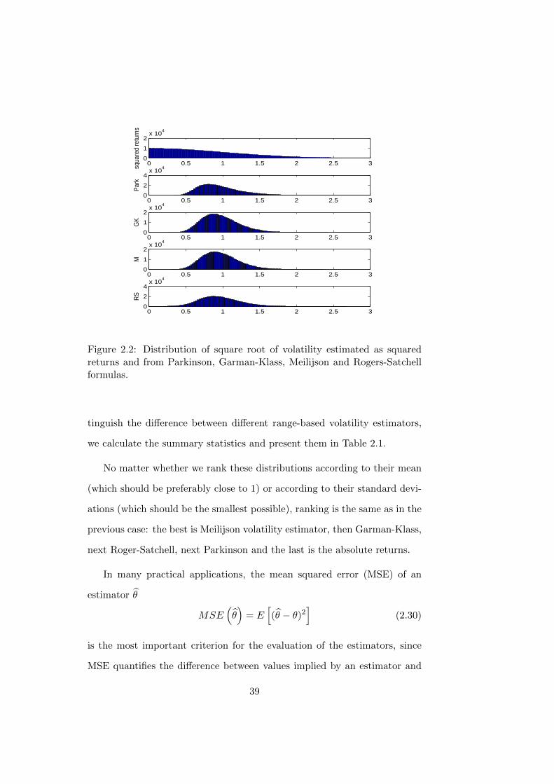
2.2 Distribution of square root of volatility estimated as squared
returns and from Parkinson, Garman-Klass, Meilijson and
Rogers-Satchell formulas. . . . . . . . . . . . . . . . . . . . . 39
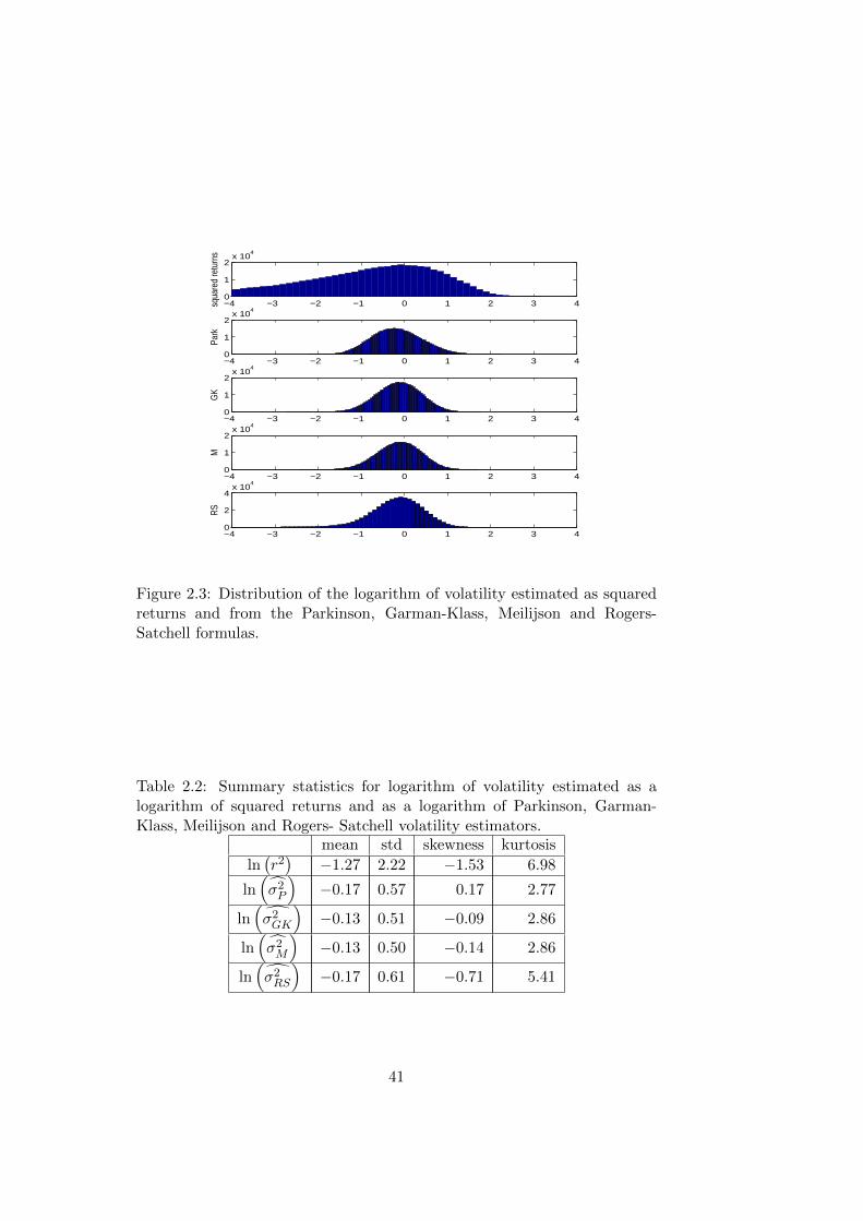
2.3 Distribution of the logarithm of volatility estimated as squared
returns and from the Parkinson, Garman-Klass, Meilijson and
Rogers-Satchell formulas. . . . . . . . . . . . . . . . . . . . . 41
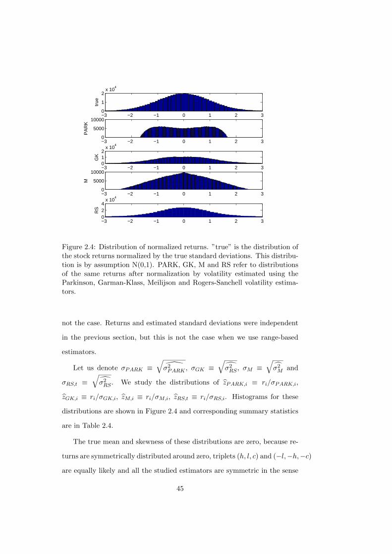
2.4 Distribution of normalized returns. ”true” is the distribution
of the stock returns normalized by the true standard devi-
ations. This distribution is by assumption N(0,1). PARK,
GK, M and RS refer to distributions of the same returns af-
ter normalization by volatility estimated using the Parkinson,
Garman-Klass, Meilijson and Rogers-Sanchell volatility esti-
mators. . . . . . . . . . . . . . . . . . . . . . . . . . . . . . . 45
v

vi
List of Tables
2.1 The summary statistics for the square root of the volatility
estimated as absolute returns and as a square root of the
Parkinson, Garman-Klass, Meilijson and Rogers-Satchell for-
mulas. . . . . . . . . . . . . . . . . . . . . . . . . . . . . . . . 40
2.2 Summary statistics for logarithm of volatility estimated as a
logarithm of squared returns and as a logarithm of Parkin-
son, Garman-Klass, Meilijson and Rogers- Satchell volatility
estimators. . . . . . . . . . . . . . . . . . . . . . . . . . . . . 41
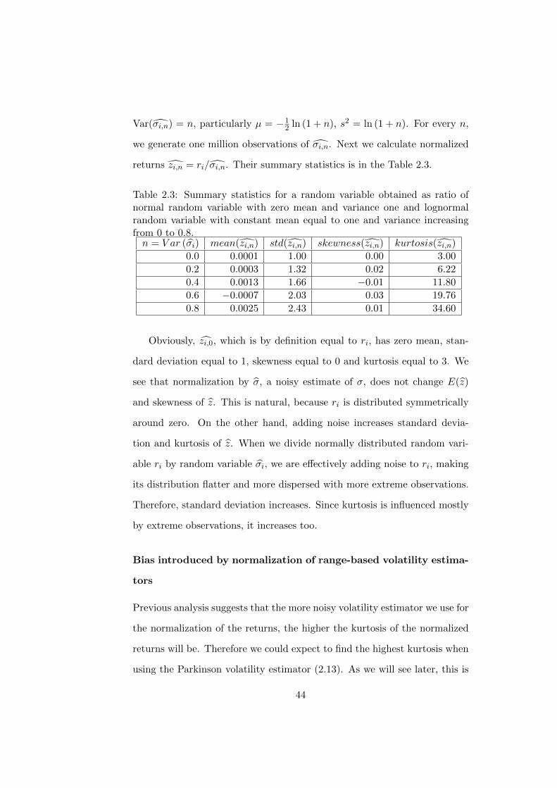
2.3 Summary statistics for a random variable obtained as ratio
of normal random variable with zero mean and variance one
and lognormal random variable with constant mean equal to
one and variance increasing from 0 to 0.8. . . . . . . . . . . . 44
2.4 Summary statistics for returns nomalized by different volatil-
ity estimates: zPARK,i ≡ ri/σPARK,i, zGK,i ≡ ri/σGK,i, zM,i ≡ri/σM,i, zRS,t ≡ ri/σRS,i. . . . . . . . . . . . . . . . . . . . . . 46
2.5 Standard deviations of the stock returns. rtd is an open-to-
close return, rd is a close-to-close return. σGK,td (σP,td) is
square root of Garman-Klass (Parkinson) volatility estimate
without opening jump component. σGK,d (σP,d) is square
root of Garman-Klass (Parkinson) volatility estimate includ-
ing opening jump component. σgarch is standard deviation
estimated from GARCH(1,1) model based on daily returns. . 53
vii
2.6 Kurtosis of the stock returns. rtd is an open-to-close return,
rd is a close-to-close return. σGK,td (σP,td) is square root of
Garman-Klass (Parkinson) volatility estimate without open-
ing jump component. σGK,d (σP,d) is square root of Garman-
Klass (Parkinson) volatility estimate including opening jump
component. σgarch is standard deviation estimated from GARCH(1,1)
model based on daily returns. . . . . . . . . . . . . . . . . . . 54
3.1 Estimated coefficients of the GARCH(1,1) model σ2t = ω +
αr2t−1+βσ2t−1 and the RGARCH(1,1) model σ2t = ω+α σ2P,t−1+
βσ2t−1, reported together with the values of Akaike Informa-
tion Criterion (AIC) of the respective equations. . . . . . . . 84
3.2 Estimated coefficients and p-values for the combined GARCH(1,1)
model σ2t = ω + α1r2t−1 + α2
σ2P,t−1 + βσ2t−1. . . . . . . . . . . 85
3.3 Comparison of the forecasting performance of the GARCH(1,1)
model σ2t = ω+αr2t−1 + βσ2t−1 and the RGARCH(1,1) model
σ2t = ω+α σ2P,t−1+βσ2t−1. Numbers in this table are 1000×RMSE
of the one-day-ahead rolling window forecast reported for dif-
ferent window sizes w. An asterisk * (**) indicates when the
difference is significant at the 5% (1%) level. . . . . . . . . . . 87
3.4 Comparison of the forecasting performance of the RGARCH(1,1)
model σ2t = ω+α σ2P,t−1 +βσ2t−1and several different GARCH
models. Numbers in this table are 1000×RMSE of the one-
day-ahead rolling window forecast with forecasting window
equal to 400. . . . . . . . . . . . . . . . . . . . . . . . . . . . 88
3.5 Comparison of forecasting performance GARCH(1,1) model
σ2t = ω + αr2t−1 + βσ2t−1 and the RGARCH(1,1) model σ2t =
ω + α σ2P,t−1 + βσ2t−1. Numbers in this table are the LLF of
the returns rt beind drawn from the distributions N(
0, σ2t
),
where σ2t is a one-day-ahead rolling window volatility forecast
reported for different window sizes w. . . . . . . . . . . . . . 92
3.6 Estimated coefficients of the GARCH(1,1) model σ2t = ω +
αr2t−1+βσ2t−1 and it modified version RGARCH(1,1) σ2t = ω+
α σ2P,t−1 + βσ2t−1, reported together with the values of Akaike
Information Criterion (AIC) of the respective equations for
the simulated data. . . . . . . . . . . . . . . . . . . . . . . . . 93
viii
3.7 Estimated coefficients and p-values for the combined GARCH(1,1)
model σ2t = ω + α1r2t−1 + α2
σ2P,t−1 + βσ2t−1. . . . . . . . . . . 93
3.8 Comparison of forecasting performance of the GARCH(1,1)
model σ2t = ω+αr2t−1+βσ2t−1 and its modified version RGARCH(1,1)
σ2t = ω+α σ2P,t−1+βσ2t−1. Numbers in this table are 1000×RMSE
of the one-day-ahead rolling window forecasts reported for
different window sizes w and different benchmarks (squared
returns r2 and the true volatility σtrue2) for the simulated data. 94
3.9 Estimated coefficients of GARCH(1,1) model σ2t = ω+αr2t−1+
βσ2t−1 and the RGARCH(1,1) model σ2t = ω+α σ2P,t−1+βσ2t−1,
reported together with the values of Akaike Information Cri-
terion (AIC) of the respective equations for the simulated data. 96
3.10 Estimated coefficients and p-values for the combined GARCH(1,1)
model σ2t = ω + α1r2t−1 + α2
σ2P,t−1 + βσ2t−1 for the simulated
data. . . . . . . . . . . . . . . . . . . . . . . . . . . . . . . . . 96
3.11 Comparison of the forecasting performance of the GARCH(1,1)
model σ2t = ω+αr2t−1+βσ2t−1 and it modified version RGARCH(1,1)
σ2t = ω+α σ2P,t−1+βσ2t−1. Numbers in this table are 1000×RMSE
of the one-day-ahead rolling window forecasts reported for
different window sizes w and different benchmarks squared
returns (r2) and the true volatility (σ2true) for the simulated
data. The differences in MSE are significant at any signifi-
cance level. . . . . . . . . . . . . . . . . . . . . . . . . . . . . 98
3.12 Estimated coefficients of the GARCH(1,1) model σ2t = ω +
αr2t−1+βσ2t−1 and the RGARCH(1,1) model σ2t = ω+α σ2P,t−1+
βσ2t−1 (both estimated on the close-to-close returns), reported
together with the values of Akaike Information Criterion (AIC)
of the respective equations. . . . . . . . . . . . . . . . . . . . 101
3.13 Estimated coefficients and p-values for the combined GARCH(1,1)
model σ2t = ω + α1r2t−1 + α2
σ2P,t−1 + βσ2t−1 estimated on the
close-to-close returns. . . . . . . . . . . . . . . . . . . . . . . . 102
ix
3.14 Comparison of the forecasting performance of the GARCH(1,1)
model σ2t = ω+αr2t−1 + βσ2t−1 and the RGARCH(1,1) model
σ2t = ω+α σ2P,t−1+βσ2t−1(both estimated on the close-to-close
returns with squared close-to-close returns as a benchmark).
Numbers in this table are 1000×RMSE of the one-day-ahead
rolling window forecast reported for different window sizes w.
An asterisk * (**) indicates when the difference is significant
at the 5% (1%) level. . . . . . . . . . . . . . . . . . . . . . . . 103
3.15 Comparison of the forecasting performance of the RGARCH(1,1)
model σ2t = ω+α σ2P,t−1 +βσ2t−1and several different GARCH
models, all of them estimated on the close-to-close returns
with squared close-to-close returns as a benchmark. Numbers
in this table are 1000×RMSE of the one-day-ahead rolling
window forecast with forecasting window equal to 400. Empty
spaces refers to cases when the used software (Eviews 7.2)
could not calculate RMSE. . . . . . . . . . . . . . . . . . . . 104
3.16 Comparison of forecasting performance GARCH(1,1) model
σ2t = ω + αr2t−1 + βσ2t−1 and the RGARCH(1,1) model σ2t =
ω + α σ2P,t−1 + βσ2t−1. Numbers in this table are the LLF of
the returns rt beind drawn from the distributions N(
0, σ2t
),
where σ2t is a one-day-ahead rolling window volatility forecast
reported for different window sizes w. . . . . . . . . . . . . . 105
3.17 Estimated coefficients of the GARCH(1,1) model σ2t = ω +
αr2t−1 + βσ2t−1 and it modified version RGARCH(1,1) σ2t =
ω + α σ2P,t−1 + βσ2t−1, both of them estimated on the close-
to-close returns, reported together with the values of Akaike
Information Criterion (AIC) of the respective equations for
various stock indices. . . . . . . . . . . . . . . . . . . . . . . . 106
3.18 Estimated coefficients and p-values for the combined GARCH(1,1)
model σ2t = ω + α1r2t−1 + α2
σ2P,t−1 + βσ2t−1 estimated on the
close-to-close returns for various stock indices. . . . . . . . . . 106
x
3.19 Comparison of forecasting performance of the GARCH(1,1)
model σ2t = ω+αr2t−1+βσ2t−1 and its modified version RGARCH(1,1)
σ2t = ω + α σ2P,t−1 + βσ2t−1 (both them estimated on the
close-to-close returns). As a benchmark is used both squared
close-to-close returns and realized variance. Numbers in this
table are 1000×RMSE of the one-day-ahead rolling window
forecasts reported for different window sizes w and different
benchmarks (squared returns r2 and the true volatility σtrue2)
for various stock indices. . . . . . . . . . . . . . . . . . . . . . 107
4.1 Bond payoff decomposition. . . . . . . . . . . . . . . . . . . . 119
4.2 Payoff to the riskless asset and to the risky bond. . . . . . . . 120
4.3 Bond in default. . . . . . . . . . . . . . . . . . . . . . . . . . 120
4.4 Values of RL using (4.19) for different values of α.
Parameter values are: RU = 8%, RF = 4%, TC = 40%, TPD =
40%, TPE = 40%, L = 60%, YD = 6%. RL,princ and RL,int refer
to tax systems where the principal and interest, respectively, are
viewed as being paid in default. (4.25) yields RL = 6.56% if one
were to use it with the same annually compounded rates and the
same values for the other parameters. . . . . . . . . . . . . . . . 127
xi

xii

Part I
Overview
1


1Introduction
1.1 Background
This dissertation attempts to contribute in two different fields: corporate fi-
nance and time-series econometrics. At the beginning of my PhD I started to
work in the field of corporate finance and the third essay of this dissertation
comes from that time. Later I became more interested in time-series econo-
metrics, particularly volatility modelling. This interest resulted in essays 1
and 2 in this dissertation and several more essays which are not completed
yet. Since my main interest during my PhD studies was volatility, I provide
3
an introduction only into the field of volatility. Since there are many good
review articles dealing with this topic (e.g. Poon and Granger (2003)), the
introduction is very brief.
1.2 Basics
Volatility as a measure of uncertainty is one of the most important variables
in economics and finance. The reason why volatility matters so much is
that economic agents are typically risk averse and future is never certain.
Volatility of different variables plays always a crucial role in any model,
whether it is a micro model describing the behavior of individuals or a
macro DSGE model describing the whole economy.
In addition to the general importance of volatility in economics, volatility
plays even a larger role in finance. In context of finance volatility typically
refers to volatility of the prices of financial assets. Volatility of asset prices
is crucial particularly in risk management, asset allocation, portfolio man-
agement and derivative pricing.
In pricing of derivative securities, whose trading volume increased man-
ifold in recent years, volatility is the most important variable. To price an
option, we need to know volatility of the underlying asset. Particularly in
case of options volatility is important to such an extent that options are now
commonly quoted in terms of volatility, not in terms of prices. Moreover, it
is possible to buy contracts on volatility itself (specified thoroughly in the
contract), or even derivatives on the volatility as an underlying asset.
First Basle Accord in 1996 basically made volatility forecasting compul-
sory for banks and many other financial institutions around the world, as
they need to fullfil capital requirements given by the value-at-risk (VaR)
methodology. VaR is defined as a minimum expected loss with a 1% (or
4
5%) confidence level. VaR estimates are easily available given the volatil-
ity forecast, the estimate of the mean return and the normal distribution
assumption. In the VaR methodology the volatility is important not only
directly, but indirectly through the assumption about the distribution of
asset returns. Before we explain this more in detail, we introduce some of
the basic concepts.
Volatility in finance refers typically either to the standard deviation or
the variance of returns. We keep this convention and when we talk about
volatility, we have in mind variance of returns. Volatility can be computed
in the following way:
σ2 =1
N − 1
N∑t=1
(rt − r)2 (1.1)
where
rt = log (Pt)− log (Pt−1) (1.2)
and r is the mean return. However, we should keep in mind that volatility
itself cannot be interpreted directly as risk. Vvolatility becomes a measure
of risk only once it is associated with some distribution, e.g. normal of
Student’s t distribution.
The main problem associated with the equation (1.1) is that this way we
can calculate only the average volatility over the studied period of time. If
volatility changes from one day to another then the usefulness of volatility
calculated in this way is limited. One of the best documented stylized facts
in finance is the fact that volatility changes over time.
1.3 Time-varying volatility
The distribution of the daily stock returns is bell-shaped with an approxi-
mately zero mean. It resembles the normal distribution. However, as has
5
already been documented by Mandelbrot (1963), they have fat (heavy) tails
to such an extent that the normality of stock returns is generally always
strongly rejected.
Clark (1973) came up with the Mixture-of-Distributions-Hypothesis (MDH)
which postulates that the distribution of returns is normal but with a ran-
dom variance. In the original formulation in Clark (1973), the variance is
assumed to be lognormally distributed. This assumption does not hold.
Volatility exhibits clustering as was noticed by researchers later. Starting
with the work of Engle (1982) and Bollerslev (1986) the Auto Regressive
Conditional Heteroskedasticity (ARCH) and Generalized ARCH classes of
models have been developed to capture the time evolution of volatility.
Engle’s (1982) ARCH(p) model has the following form:
σ2t = ω +
p∑i=1
αir2t−i (1.3)
where rt is a return in day t, σ2t is an estimate of volatility in day t and
ω and αi’s are positive constants. The GARCH(p,q) model of Bollerslev
(1986) has the following form:
σ2t = ω +
p∑i=1
αir2t−i +
q∑j=1
βiσ2t−j (1.4)
where the βi’s are positive constants. The GARCH model has become more
popular because with just a few parameters it can fit the data better than
a more parametrized ARCH model. Afterwards, GARCH models were ex-
tended to capture the leverage effect. The leverage effect is an empirically
observed fact that volatility increases after negative returns. (One of the
possible explanations of the leverage effect is based on the fact that equity
is a residual claim on the value of the company). GARCH models were de-
6
veloped further to incorporate long memory in volatility, regime switching
and other effects.
An alternative way to capture the properties of stock returns is to use
stochastic volatility models instead of GARCH models. Stochastic volatility
models were first introduced by Taylor (1973). The main difference be-
tween stochastic volatility models and GARCH models is the following one.
Innovations to volatility in GARCH models are given by returns, whereas
innovations to volatility in stochastic volatility models might be completely
unrelated to returns.1
Therefore stochastic volatility models can be considered more general
than GARCH models. However, GARCH models still remain the most
widely used volatility models. The reason for this is the fact that GARCH
models can be estimated easily via the maximum likelihood, whereas the es-
timation of stochastic volatility models must be done using more complicated
techniques (e.g. Kalman filter, quasi-maximum likelihood, the generalized
method of moments through simulations, Monte Carlo simulations).
1.4 Conditional distribution of stock returns
The ARCH/GARCH models are able to explain heavy tails in stock returns
only partially. These models are still unable to account for all of the mass in
the tails of the distributions, leaving the conditional distribution of returns
far from normal. To better account for the deviations from the normality
in the conditional distributions of returns, alternative conditional distri-
butions with heavy tails (e.g. the t-distribution of Bollerslev (1987), the
General Error Distribution (GED) of Nelson (1991) and more recently, the
1However, these two are in most models correlated, as this correlation produces theleverage effect, which is observed in the data.
7
Normal Inverse Gaussian (NIG) distribution of Barndorff-Nielsen (1997))
were suggested for stock returns.
However, the idea of the normality of conditional stock returns was not
forgotten. The emergence of the high frequency data allowed to calculate
the realized variance, a very precise estimate of the true variance. Using
the realized variance, several authors (e.g. Andersen, Bollerslev, Diebold,
Labys (2000), Andersen, Bollerslev, Diebold, Ebens (2001), Forsberg and
Bollerslev (2002) and Thamakos and Wang (2003)) showed on different data
sets that the conditional distribution of asset returns (i.e. the distribution of
asset returns divided by their standard deviations) is indeed approximately
normal. Even though the asymmetry of stock returns is a well documented
fact (see e.g. Longin and Solnik (2000), Ang and Chen (2002)) it can be
considered a second-order effect.
The finding that most of the departure from normality is caused by time-
varying volatility not only allows us to understand financial markets better
but this insight allows us to develop better volatility models. If we have a
model which predicts volatility perfectly then the conditional distribution
of stock returns will be approximately normal. If volatility is forecasted
imperfectly then the conditional distribution of returns will exhibit heavy
tails. Since no model can predict future volatility perfectly heavy-tailed
distributions will still be needed in volatility forecasting. However, the more
precise is the volatility model the closer will be the distribution of returns
to the normal distribution.
1.5 Implied volatility
There are two other volatility concepts which should be mentioned: the
implied volatility and the realized variance. Implied volatility is volatility
8
implied by option prices. It is necessarily forward looking; it captures the
expectations of market participants about future volatility. Therefore, it
is generally quite useful in volatility forecasting. However, we must keep
in mind that a test of the forecasting power of the implied volatility is
necessarily a joint test of the option market efficiency and the correct option
pricing model.
Black-Scholes (1973) option pricing formula assumes that the growth
rate of stock follows a Brownian motion with drift
dS
S= µdt+ σdBt. (1.5)
Further assumptions include: constant volatility, no transaction costs, per-
fectly divisible securities, no arbitrage, a constant risk-free rate and no div-
idends. Given these assumptions, the Black-scholes option pricing formula
for the European option at time t is a function of the price of the underlying
security St, the maturity of the option T , volatility σ of the underlying asset
from time t to T , the risk-free interest rate r and the strike price X:
C = f (St, X, σ, r, t− T ) (1.6)
Therefore once the market has produced the price of the option, the rela-
tionship (1.6) can be inverted and we can infer volatility which was the input
into this formula. Since the underlying asset can have only one volatility,
options of the same time to maturity but different strike prices should im-
ply the same volatility. However, this is typically not the case. Plots of
implied volatility against the strike price are usually not flat, but instead
create a nonlinear shape (volatility smile, volatility skew or something else).
Several explanations have been suggested to explain this phenomenon (dis-
9
tributional assumptions, stochastic volatility, liquidity, bid-ask spread, tick
size, investors’ risk preferences,...).
Due to the above mentioned effects implied volatility is usually calculated
from at-the-money options (for example the best known implied volatility
index VIX is calculated by combining just-in-the-money and just-out-of-the-
money options, both put and call options). Implied volatility is typically
very useful as it provides information beyond the historical prices, but it
is available only for the financial instruments which are used as underlying
assets for options, and those options must have sufficient liquidity.
1.6 Realized variance
The realized variance is the estimate of volatility calculated from the high-
frequency data. If log-returns (pt = log (Pt)) are generated by a Brownian
motion, for simplicity with a zero drift
dpt = σtdBt (1.7)
then the volatility of one-period returns rt = pt+1 − pt can be calculated as
the integrated volatility∫ 10 σ
2t+τdτ . However, in practical applications we
cannot observe the variable σ2t+τ . Moreover, no variable can be observed
continuously. As a consequence, the integrated volatility is replaced by the
realized variance. If we divide the time interval from time t to time t+1 into
M subintervals and denote the corresponding returns as rm,m+1, then the
realized variance is calculated as the sum of squared returnsM−1∑0r2m,m+1. In
other words, to calculate the realized variance for a given day, first divide
the day into many short intervals, calculate returns over those intervals,
square these returns and sum these squares up. Theoretically, the shorter
10
are the intervals, the more precise is the final estimate. However, due to
market microstructure effects (mostly the bid-ask spread), very short time
intervals cannot be chosen. Intervals of the length of 5 to 30 minutes are
typically used. Alternatively, more sophisticated estimators could be used
instead (e.g. Zhang, Mykland and Ait-Sahalia (2005))
The realized variance provides quite precise estimates of volatility during
a particular day. The largest limitation of the realized variance is the data
availability. The high-frequency data are typically costly to obtain and work
with. Moreover, for longer time horizons (i.e. further into the past) high-
frequency data not available at all.
1.7 Range-based volatility estimators
Standard GARCH or stochastic volatility models are based on daily returns.
However, the closing price of the day is typically not the only quantity
available. Denote the price at the beginning of the day (i.e. at the time
t = 0) O (open), the price in the end of the day (i.e. at the time t = 1)
C (close), the highest price of the day H, and the lowest price of the day
L. These prices are usually widely available too. Then we can calculate the
open-to-close, the open-to-high and the open-to-low returns as
c = ln(C)− ln(O) (1.8)
h = ln(H)− ln(O) (1.9)
l = ln(L)− ln(O) (1.10)
11
When we want to estimate the (unobservable) volatility σ2 from the observed
variables c, h and l, we can obviously use a simple volatility estimator
σ2s = c2 (1.11)
However, this simple estimator is very noisy and therefore it is desirable to
have a better one. Fortunately, the high and low prices not only provide
additional information about volatility but it is also intuitively clear that the
difference between the high and low price tells us much more about volatility
than the close price. This intuition was formalized by Parkinson (1980), who
proposed a new volatility estimator based on the range (= h− l):
σ2P =(h− l)2
4 ln 2(1.12)
Since this estimator is based solely on the quantity h− l Garman and Klass
(1980) realized that an estimator which utilizes all the available information
c, h and l will be necessarily more precise. They recommend to use the
following volatility estimator:
σ2GK = 0.5 (h− l)2 − (2 ln 2− 1) c2 (1.13)
This estimator can be simply interpreted as the optimal (i.e. giving the
smallest variance) combination of the simple and the Parkinson volatility
estimator. Other range-based estimators are Meilijson (2009) and Rogers
and Satchell (1991) estimators. The Rogers and Satchell (1991) estimator
allows for an arbitrary drift, but provides less precision than the other esti-
mators. The Meilijson (2009) estimator is a slightly improved version of the
Garman-Klass volatility estimator. All of the studied estimators except for
12
the Rogers-Satchell are derived under the assumption of zero drift. However,
for most of the financial assets, the mean daily return is much smaller than
its standard deviation and can therefore be neglected. Obviously, this is not
true for longer time horizons (e.g. when we use yearly data), but is a very
good approximation for daily data in basically any practical application.
Range and range-based volatility estimators provide a convenient way
to improve volatility models. Literature has started to grow in this field
recently. Alizadeh, Brandt and Diebold (2002) estimate a stochastic volatil-
ity model. Brandt and Jones (2006) estimate EGARCH and FIEGARCH
models based on log range. Chou (2005) uses range in standard deviation
GARCH. Good overview of range volatility models and their applications in
Finance can be found in Chou, Chou and Liu (2010).
1.8 Summaries
1.8.1 Properties of range-based volatility estimators
accepted for publication in the International Review of Financial Analysis
In this first essay I study the properties of various range-based volatility
estimators. One of the reasons for this essay was that there was some confu-
sion about some of their properties. We study the properties of range-based
volatility estimators and clarify some problems in the existing literature. We
find that for most purposes the Garman-Klass (1980) volatility estimator is
the best. Moreover, we show that this estimator is precise enough to obtain
results similar to the realized variance. More specifically, we show that the
returns standardized by standard deviations obtained from this estimator
are approximately normally distributed.
I used the knowledge obtained during the work on this essay in other
13
essays, particularly in the second essay in this dissertation and other essays
which are not part of this dissertation.
1.8.2 Rethinking the GARCH
The goal of this essay was to create a more precise but at the same time
an easy-to-implement volatility model which can be easily used by anyone.
This was accomplished by incorporating information on range into standard
GARCH(1,1) model. The empirical analysis based on 30 stocks, 6 stock
indices and simulated data confirms that the Range GARCH model performs
significantly better than the standard GARCH(1,1) model regarding both
the in-sample fit and the out-of-sample forecasting performance.
1.8.3 Tax-Adjusted Discount Rates: A General Formula un-
der Constant Leverage Ratios
with Kjell G. Nyborg
accepted for publication in the European Financial Management
In this paper we derive a general formula how to calculate a discount rate
for discounting of the expected cash flow of the company when we take into
account personal taxes. If there are no personal taxes the well-known con-
cept of Weighted Average Capital Costs provides an answer. However, the
situation become less clear once personal taxes are not neglected. Cooper
and Nyborg (2008) derive a tax-adjusted discount rate formula under in-
vestor taxes (and a constant proportion leverage policy). However, their
analysis assumes a zero recovery in default and a particular bankruptcy
code. We extend their work to allow for differences in bankruptcy codes
(which affect the taxes) and for an arbitrary recovery rate in default.
The general formula we derive is a generalization of Cooper and Nyborg
14

(2008). However, the formula collapses to that of Cooper and Nyborg under
continuous rebalancing. This means that there is no recovery rate in the
final formula. However, we explain that this does not mean that the discount
rate is independent of the anticipated recovery rate. Instead, the anticipated
recovery rate is already reflected in the yield of the bond.
15

16
Bibliography
[1] Alizadeh, S., Brandt, M. W., and Diebold, F. X. (2002). “Range-based
estimation of stochastic volatility models.”Journal of Finance, 57, 1047–
1091.
[2] Andersen, T. G., Bollerslev, T. Diebold F.X. and Ebens, H. (2001).
“The distribution of realized stock return volatility.”Journal of Finan-
cial Economics, 61, 43–76.
[3] Andersen T.G., Bollerslev T., Diebold F.X., Labys P. (2000). “Ex-
change rate returns standardized by realized volatility are nearly Gaus-
sian.”Multinational Finance Journal, 4, 159–179.
[4] Ang, Andrew, and Chen, Joseph, (2002), “Asymmetric Correlations of
Equity Portfolios”, Journal of Financial Economics, 63(3), 443–494.
[5] Black, F. and Scholes, M., (1973). “The Pricing of Options and Corpo-
rate Liabilities”, Journal of Political Economy 81, 637–V54
[6] Bollerslev, T. (1986). “Generalized Autoregressive Conditional Het-
eroscedasticity.”Journal of Econometrics 31, 307–327.
17
[7] Bollerslev, T.(1987). “A Conditionally Heteroskedastic Time Series
Model for Speculative Prices and Rates of Return,”Rev. Econ. Statist.
69:3, pp. 542–547.
[8] Brandt, M. W. Christopher S. Jones, Ch. S., (2006). “Volatility fore-
casting with Range-Based EGARCH models.”Journal of Business and
Economic Statistics, 24(4): 470–486.
[9] Clark, P. (1973). “A Subordinated Stochastic Process Model with Finite
Variance for Speculative Prices, Econometrica 41, pp. 135V56
[10] Chou, R.Y. (2005) “Forecasting financial volatilities with extreme val-
ues: the conditional autoregressive range (CARR) model.”Journal of
Money, Credit and Banking 37(3): 561–582.
[11] Chou, Y. Ray, Hengchin Chou, and Nathan Liu, 2010, “The economic
value of volatility timing using a range-based volatility model, Journal
of Economic Dynamics and Control, 2288–2301.
[12] Cooper, I.A. and K.G. Nyborg, 2008, “Tax-Adjusted Discount Rates
With Investor Taxes and Risky Debt”, Financial Management, Summer
2008, 365–379
[13] Engle, Robert (1982). “Autoregressive Conditional Heteroscedasticity
with Estimates of the Variance of U.K. Inflation.” Econometrica 50,
987–1008.
[14] Forsberg, L. and Bollerslev, T. (2002), “Bridging the gap between the
distribution of realized (ECU) volatility and ARCH modelling (of the
Euro): the GARCH-NIG model.”Journal of Applied Econometrics, 17:
535–548.
18
[15] Garman, Mark B. and Klass, Michael J., (1980), “On the Estimation of
Security Price Volatilities from Historical Data”, The Journal of Busi-
ness, Vol. 53, No. 1, 67-7
[16] Longin, Francois, and Solnik, Bruno, 2001, “Extreme Correlation of
International Equity Markets”, Journal of Finance, 56, 649-676.
[17] Mandelbrot, Benoit B. (1963), “The variation of certain speculative
prices.”Journal of Business 36, 394.419.
[18] Meilijson, I., (2009), “The Garman–Klass volatil-
ity estimator revisited.”, working paper available at:
http://arxiv.org/PS cache/arxiv/pdf/0807/0807.3492v2.pdf
[19] Nelson, Daniel B., 1991, “Conditional heteroskedasticity in asset pric-
ing: A new approach.”Econometrica 59, 347-370.
[20] Parkinson, M. (1980). “The extreme value method for estimating the
variance of the rate of return.”Journal of Business, 53, 61–65.
[21] Poon, Ser-Huang and Clive W. Granger (2003), “Forecasting Volatility
in Financial Markets: a Review.”Journal of Economic Literature, Vol.
41 (June 2003), pp. 478–539
[22] Rogers, L. C. G., and Satchell, S. E. 1991. “Estimating variance from
high, low and closing prices.”Annals of Applied Probability 1: 504–12.
[23] Taylor, S.J. (1986), “Modeling Financial Time Series.”Chichester, UK:
John Wiley and Sons.
[24] Thomakos, D. D., Wang, T., (2003), “Realized volatility in the futures
markets”, Journal of Empirical Finance, 10, 321–353.
19

[25] Zhang, L., Myykland, P. and Ait-Sahalia, Y. (2005), “A Tale of
Two Time Scales: Determining Integrated Volatility with Noisy High-
Frequency Data”, Journal of the American Statistical Association, 100,
1394–1411.
20

Part II
Essays
21

2Properties of range-based volatility
estimators
23
Abstract
Volatility is not directly observable and must be estimated. Estimator based
on daily close data is imprecise. Range-based volatility estimators provide
significantly more precision, but still remain noisy volatility estimates, some-
thing that is sometimes forgotten when these estimators are used in further
calculations.
First, we analyze properties of these estimators and find that the best
estimator is the Garman-Klass (1980) estimator. Second, we correct some
mistakes in existing literature. Third, the use of the Garman-Klass estima-
tor allows us to obtain an interesting result: returns normalized by their
standard deviations are approximately normally distributed. This result,
which is in line with results obtained from high frequency data, but has
never previously been recognized in low frequency (daily) data, is important
for building simpler and more precise volatility models.
Key words: volatility, high, low, range
JEL Classification: C58, G17, G32 1
1I would like to thank to Jonas Andersson, Milan Basta, Ove Rein Hetland, LukasLaffers, Michal Zdenek and anonymous referees for helpful comments.
24
2.1 Introduction
Asset volatility, a measure of risk, plays a crucial role in many areas of
finance and economics. Therefore, volatility modelling and forecasting be-
come one of the most developed parts of financial econometrics. However,
since the volatility is not directly observable, the first problem which must be
dealt with before modelling or forecasting is always a volatility measurement
(or, more precisely, estimation).
Consider stock price over several days. From a statistician’s point of
view, daily relative changes of stock price (stock returns) are almost random.
Moreover, even though daily stock returns are typically of a magnitude of 1%
or 2%, they are approximately equally often positive and negative, making
average daily return very close to zero. The most natural measure for huw
much stock price changes is the variance of the stock returns. Variance can
be easily calculated and it is a natural measure of the volatility. However,
this way we can get only an average volatility over an investigated time
period. This might not be sufficient, because volatility changes from one
day to another. When we have daily closing prices and we need to estimate
volatility on a daily basis, the only estimate we have is squared (demeaned)
daily return. This estimate is very noisy, but since it is very often the
only one we have, it is commonly used. In fact, we can look at most of
the volatility models (e.g. GARCH class of models or stochastic volatility
models) in such a way that daily volatility is first estimated as squared
returns and consequently processed by applying time series techniques.
When not only daily closing prices, but intraday high frequency data are
available too, we can estimate daily volatility more precisely. However, high
frequency data are in many cases not available at all or available only over a
shorter time horizon and costly to obtain and work with. Moreover, due to
25
market microstructure effects the volatility estimation from high frequency
data is rather a complex issue (see Dacorogna et al. 2001).
However, closing prices are not the only easily available daily data. For
the most of financial assets, daily open, high and low prices are available too.
Range, the difference between high and low prices is a natural candidate for
the volatility estimation. The assumption that the stock return follows a
Brownian motion with zero drift during the day allows Parkinson (1980)
to formalize this intuition and derive a volatility estimator for the diffusion
parameter of the Brownian motion. This estimator based on the range (the
difference between high and low prices) is much less noisy than squared
returns. Garman and Klass (1980) subsequently introduce estimator based
on open, high, low and close prices, which is even less noisy. Even though
these estimators have existed for more than 30 years, they have been rarely
used in the past by both academics and practitioners. However, recently the
literature using the range-based volatility estimators started to grow (e.g.
Alizadeh, Brandt and Diebold (2002), Brandt and Diebold (2006), Brandt
and Jones (2006), Chou (2005), Chou (2006), Chou and Liu (2010)). For an
overview see Chou, Chou and Liu (2010).
Despite increased interest in the range-based estimators, their properties
are sometimes somewhat imprecisely understood. One particular problem
is that despite the increased accuracy of these estimators in comparison
to squared returns, these estimators still only provide a noisy estimate of
volatility. However, in some manipulations (e.g. division) people treat these
estimators as if they were exact values of the volatility. This can in turns
lead to flawed conclusions, as we show later in the paper. Therefore we
study these properties.
Our contributions are the following. First, when the underlying assump-
26
tions of the range-based estimators hold, all of them are unbiased. However,
taking the square root of these estimators leads to biased estimators of
standard deviation. We study this bias. Second, for a given true variance,
distribution of the estimated variance depends on the particular estimator.
We study these distributions. Third, we show how the range-based volatility
estimators should be modified in the presence of opening jumps (stock price
at the beginning of the day typically differs from the closing stock price from
the previous day).
Fourth, the property we focus on is the distribution of returns stan-
dardized by standard deviations. A question of interest is how this is af-
fected when the standard deviations are estimated from range-based volatil-
ity estimators. The question whether the returns divided by their standard
deviations are normally distributed has important implications for many
fields in finance. Normality of returns standardized by their standard de-
viations holds promise for simple-to-implement and yet precise models in
financial risk management. Using volatility estimated from high frequency
data, Andersen, Bollerslev, Diebold and Labys (2000), Andersen, Bollerslev,
Diebold, Ebens (2001), Forsberg and Bollerslev (2002) and Thamakos and
Wang (2003) show that standardized returns are indeed Gaussian. Contrary,
returns scaled by standard deviations estimated from GARCH type of mod-
els (which are based on daily returns) are not Gaussian, they have heavy
tails. This well-known fact is the reason why heavy-tailed distributions (e.g.
t-distribution) were introduced into the GARCH models. We show that
when properly used, range-based volatility estimators are precise enough to
replicate basically the same results as those of Andersen et al. (2001) ob-
tained from high frequency data. To our best knowledge, this has not been
previously recognized in the daily data. Therefore volatility models built
27
upon high and low data might provide accuracy similar to models based
upon high frequency data and still keep the benefits of the models based on
low frequency data (much smaller data requirements and simplicity).
The rest of the paper is organized in the following way. In Section 2, we
describe existing range-based volatility estimators. In Section 3, we analyze
properties of range-based volatility estimators, mention some caveats related
to them and correct some mistakes in the existing literature. In Section 4 we
empirically study the distribution of returns normalized by their standard
deviations (estimated from range-based volatility estimators) on 30 stock,
the components of the Dow Jones Industrial Average. Section 5 concludes.
2.2 Overview
Assume that price P follows a geometric Brownian motion such that log-
price p = ln(P ) follows a Brownian motion with zero drift and diffusion
σ.
dpt = σdBt (2.1)
Diffusion parameter σ is assumed to be constant during one particular day,
but can change from one day to another. We use one day as a unit of time.
This normalization means that the diffusion parameter in (2.1) coincides
with the daily standard deviation of returns and we do not need to distin-
guish between these two quantities. Denote the price at the beginning of the
day (i.e. at the time t = 0) O (open), the price in the end of the day (i.e.
at the time t = 1) C (close), the highest price of the day H, and the lowest
price of the day L. Then we can calculate open-to-close, open-to-high and
open-to-low returns as
c = ln(C)− ln(O) (2.2)
28
h = ln(H)− ln(O) (2.3)
l = ln(L)− ln(O) (2.4)
Daily return c is obviously a random variable drawn from a normal distri-
bution with zero mean and variance (volatility) σ2
c ∼ N(0, σ2) (2.5)
Our goal is to estimate (unobservable) volatility σ2 from observed variables
c, h and l. Since we know that c2 is an unbiased estimator of σ2,
E(c2)
= σ2 (2.6)
we have the first volatility estimator (subscript s stands for ”simple”)
σ2s = c2 (2.7)
Since this simple estimator is very noisy, it is desirable to have a better one.
It is intuitively clear that the difference between high and low prices tells us
much more about volatility than close price. High and low prices provide
additional information about volatility. The distribution of the range d ≡
h− l (the difference between the highest and the lowest value) of Brownian
motion is known (Feller (1951)). Define P (x) to be the probability that
d ≤ x during the day. Then
P (x) =
∞∑n=1
(−1)n+1 n
{Erfc
((n+ 1)x√
2σ
)− 2Erfc
(nx√2σ
)+ Erfc
((n− 1)x√
2σ
)}(2.8)
29
where
Erfc(x) = 1− Erf(x) (2.9)
and Erf(x) is the error function. Using this distribution Parkinson (1980)
calculates (for p ≥ 1)
E (dp) =4√π
Γ
(p+ 1
2
)(1− 4
2p
)ζ (p− 1)
(2σ2)
(2.10)
where Γ (x) is the gamma function and ζ (x) is the Riemann zeta function.
Particularly for p = 1
E (d) =√
8πσ (2.11)
and for p = 2
E(d2)
= 4 ln (2)σ2 (2.12)
Based on formula (2.12), he proposes a new volatility estimator:
σ2P =(h− l)2
4 ln 2(2.13)
Garman and Klass (1980) realize that this estimator is based solely on
quantity h − l and therefore an estimator which utilizes all the available
information c, h and l will be necessarily more precise. Since search for the
minimum variance estimator based on c, h and l is an infinite dimensional
problem, they restrict this problem to analytica estimators, i.e. estimators
which can be expressed as an analytical function of c, h and l. They find
that the minimum variance analytical estimator is given by the formula
σ2GKprecise = 0.511 (h− l)2 − 0.019 (c(h+ l)− 2hl)− 0.383c2 (2.14)
The second term (cross-products) is very small and therefore they recom-
30
mend neglecting it and using more practical estimator:
σ2GK = 0.5 (h− l)2 − (2 ln 2− 1) c2 (2.15)
We follow their advice and further on when we talk about Garman-Klass
volatility estimator (GK), we refer to (2.15). This estimator has additional
advantage over (2.14) - it can be simply explained as an optimal (smallest
variance) combination of simple and Parkinson volatility estimator.
Meilijson (2009) derives another estimator, outside the class of analytical
estimators, which has even smaller variance than GK. This estimator is
constructed as follows.
σ2M = 0.274σ21 + 0.16σ2s + 0.365σ23 + 0.2σ24 (2.16)
where
σ21 = 2[(h′ − c′
)2+ l′]
(2.17)
σ23 = 2(h′ − c′ − l′
)c′ (2.18)
σ24 = − (h′ − c′) l′
2 ln 2− 5/4(2.19)
where c′ = c, h′ = h, l′ = l if c > 0 and c′ = −c, h′ = −l, l′ = −h if c < 0.2
Rogers and Satchell (1991) derive an estimator which allows for arbitrary
drift.
σ2RS = h(h− c) + l(l − c) (2.20)
There are two other estimators which we should mention. Kunitomo
(1992) derives a drift-independent estimator, which is more precise than
all the previously mentioned estimators. However ”high” and ”low” prices
2This estimator is not analytical, because it uses different formula for days when c > 0than for days when c < 0.
31
used in his estimator are not the highest and lowest price of the day. The
”high” and ”low” used in this estimator are the highest and the lowest price
relative to the trend line given by open and high prices. These ”high and
”low” prices are unknown unless we have tick-by-tick data and therefore the
use of this estimator is very limited.
Yang and Zhang (2000) derive another drift-independent estimator. How-
ever, their estimator can be used only for estimation of average volatility
over multiple days and therefore we do not study it in our paper.
Efficiency of a volatility estimator σ2 is defined as
Eff(σ2) ≡var
(σ2s)
var(σ2) (2.21)
Simple volatility estimator has by definition efficiency 1, Parkinson volatility
estimator has efficiency 4.9, Garman-Klass 7.4 and Meilijson 7.7. Rogers,
Satchell has efficiency 6.0 for the zero drift and larger than 2 for any drift.
Remember that all of the studied estimators except for Rogers, Satchell
are derived under the assumption of zero drift. However, for most of the
financial assets, mean daily return is much smaller than its standard devi-
ation and can therefore be neglected. Obviously, this is not true for longer
time horizons (e.g. when we use yearly data), but this is a very good ap-
proximation for daily data in basically any practical application.
Further assumptions behind these estimators are continuous sampling,
no bid-ask spread and constant volatility. If prices are observed only infre-
quently, then the observed high will be below the true high and observed
low will be above the true low, as was recognized already by Garman and
Klass (1980). Bid-ask spread has the opposite effect: observed high price
is likely to happen at ask, observed low price is likely to happen at the low
32
price and therefore the difference between high and low contains in addition
bid-ask spread. These effects work in the opposite direction and therefore
they will at least partially cancel out. More importantly, for liquid stocks
both these effects are very small. In this paper we maintain the assump-
tion of constant volatility within the day. This approach is common even in
stochastic volatility literature (e.g. Alizadeh, Brandt and Diebold 2002) and
assessing the effect of departing from this assumption is beyond the scope
of this paper. However, this is an interesting avenue for further research.
2.3 Properties of range-based volatility estimators
The previous section provided an overview of range-based volatility estima-
tors including their efficiency. Here we study their other properties. Our
main focus is not their empirical performance, as this question has been
studied before (e.g. Bali and Weinbaum (2005)). We study the performance
of these estimators when all the assumptions of these estimators hold per-
fectly. This is more important than it seems to be, because this allows us to
distinguish between the case when these estimators do not work (assump-
tions behind them do not hold) and the case when these estimators work,
but we are misinterpreting the results. This point can be illustrated in the
following example. Imagine that we want to study the distribution of returns
standardized by their standard deviations. We estimate these standard de-
viations as a square root of the Parkinson volatility estimator (2.13) and find
that standardized returns are not normally distributed. Should we conclude
that true standardized returns are not normally distributed or should we
conclude that the Parkinson volatility estimator is not appropriate for this
purpose? We answer this and other related questions.
To do so, we ran 500000 simulations, one simulation representing one
33
trading day. During every trading day log-price p follows a Brownian mo-
tion with zero drift and daily diffusion σ = 1. We approximate continuous
Brownian motion by n = 100000 discrete intraday returns, each drawn from
N(0, 1/√n).3 We save high, low and close log-prices h, l, c for every trading
day4.
2.3.1 Bias in σ
All the previously mentioned estimators are unbiased estimators of σ2. There-
fore, square root of any of these estimators will be a biased estimator of σ.
This is direct consequence of well known fact that for a random variable
x the quantities E(x2) and E(x)2 are generally different. However, as I
document later, using√σ2 as σ, as an estimator of σ, is not uncommon.
Moreover, in many cases the objects of our interests are standard deviations,
not variances. Therefore, it is important to understand the size of the error
introduced by using√σ2 instead of σ and potentially correct for this bias.
Size of this bias depends on the particular estimator.
As can be easily proved, an unbiased estimator σs of the standard devi-
ation σ based on
√σ2s is
σs =
√σ2s ×
√π
2= |c| ×
√π/2 (2.22)
Using the results (2.11) and (2.13) we can easily find that an estimator of
3Such a high n allows us to have almost perfectly continuous Brownian motion andhaving so many trading days allow us to know the distributions of range based volatilityestimators with very high precision. Simulating these data took one months on an ordinarycomputer (Intel Core 2 Duo P8600 2.4 GHz, 2 GB RAM).
Note that we do not derive analytical formulas for the distributions of range-basedvolatility estimators. Since these formulas would not bring additional insights into thequestions we study, their derivation is behind the scope of this paper.
4Open log-price is normalized to zero.
34
standard deviation based on range is
σP =h− l
2×√π
2=
√σ2P ×
√π ln 2
2(2.23)
Similarly, when we want to evaluate the bias introduced by using√σ2 in-
stead of σ for the rest of volatility estimators, we want to find constants
cGK , cM and cRS such that
σGK =
√σ2GK × cGK (2.24)
σM =
√σ2M × cM (2.25)
σRS =
√σ2RS × cRS (2.26)
From simulated high, low and close log-prices h, l, c we estimate volatility
according to (2.7), (2.13), (2.15), (2.16), (2.20) and calculate mean of the
square root of these volatility estimates. We find that cs = 1.253, cP =
1.043 (what is in accordance with theoretical values√π/2 = 1.253 and√
π ln 2/2 = 1.043) and cGK = 1.034, cM = 1.033 and cRS = 1.043. We see
that the square root of the simple volatility estimator is a severely biased
estimator of standard deviation (bias is 25%), whereas bias in the square
root of range-based volatility estimators is rather small (3% - 4%).
Even though it seems obvious that√σ2 is not an unbiased estimator of
σ, it is quite common even among researchers to use√σ2 as an estimator
of σ. I document this in two examples.
Bali and Weinbaum (2005) empirically compare range-based volatility
estimators. The criteria they use are: mean squared error
MSE (σestimated) = E[(σestimated − σtrue)2
](2.27)
35
mean absolute deviation
MAD (σestimated) = E [|σestimated − σtrue|] (2.28)
and proportional bias
Prop.Bias (σestimated) = E [(σestimated − σtrue)/σtrue] (2.29)
For daily returns they find:
”The traditional estimator [(2.7) in our paper] is significantly
biased in all four data sets. [...] it was found that squared returns
do not provide unbiased estimates of the ex post realized volatil-
ity. Of particular interest, across the four data sets, extreme-
value volatility estimators are almost always significantly less
biased than the traditional estimator.”
This conclusion sounds surprising only until we realize that in their calcu-
lations σestimated ≡√σ2, which, as just shown, is not an unbiased estimator
of σ. Actually, it is severely biased for a simple volatility estimator. Gener-
ally, if our interest is unbiased estimate of the standard deviation, we should
use formulas (2.22)-(2.26).
A similar problem is in Bollen, Inder (2002). In testing for the bias in
the estimators of σ, they correctly adjust
√σ2s using formula (2.22), but
they do not adjust
√σ2P and
√σ2GK by constants cP and cGK .
2.3.2 Distributional properties of range-based estimators
Daily volatility estimates are typically further used in volatility models.
Ease of the estimation of these models depends not only on the efficiency of
36
the used volatility estimator, but on its distributional properties too (Broto,
Ruiz (2004)). When the estimates of relevant volatility measure (whether
it is σ2, σ or lnσ2) have approximately normal distribution, the volatility
models can be estimated more easily.5 We study the distributions of σ2,√σ2
and ln σ2, because these are the quantities modelled by volatility models.
Most of the GARCH models try to capture time evolution of σ2, EGARCH
and stochastic volatility models are based on time evolution of lnσ2 and
some GARCH models model time evolution of σ.
Under the assumption of Brownian motion, the distribution of absolute
value of return and the distribution of range are known (Karatzas and Shreve
(1991), Feller (1951)). Using their result, Alizadeh, Brandt, Diebold (2002)
derive the distribution of log absolute return and log range. Distribution
of σ2,√σ2 and ln σ2 is unknown for the rest of the range-based volatility
estimators. Therefore we study these distributions. To do this, we use
numerical evaluation of h, l and c data, which are simulated according to
the process (2.1) (.6
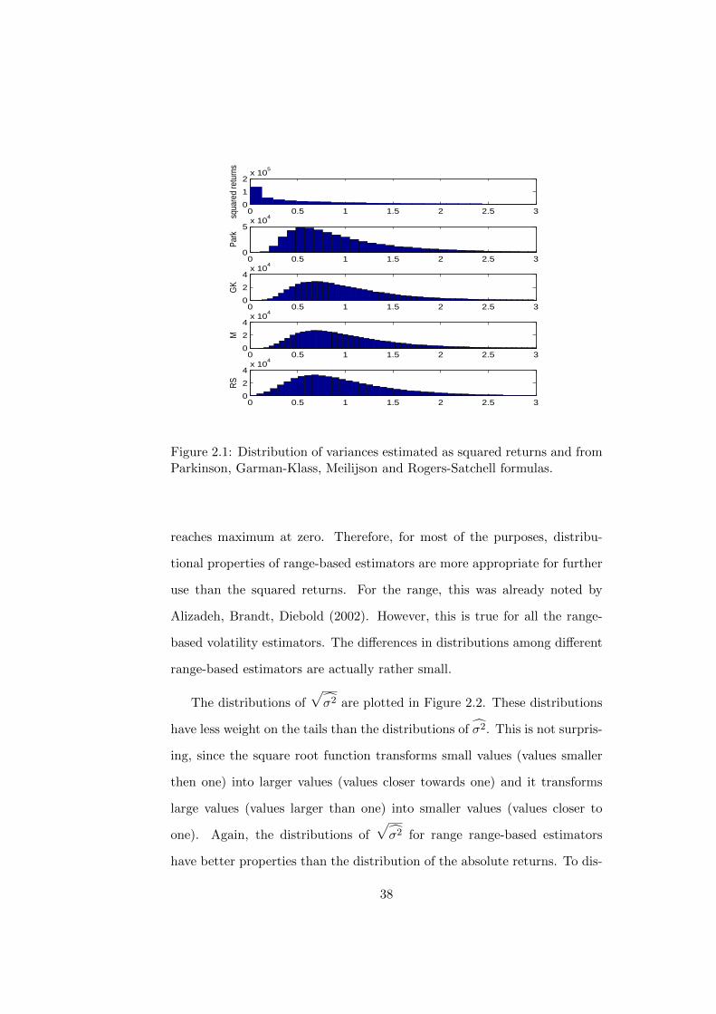
First we study the distribution of σ2 for different estimators. These dis-
tributions are plotted in Figure 2.1. Since all these estimators are unbiased
estimators of σ2, all have the same mean (in our case one). Variance of these
estimators is given by their efficiency. From the inspection of Figure 2.1, we
can observe that the density function of σ2 is approximately lognormal for
range-based estimators. On the other hand, distribution of squared returns,
which is χ2 distribution with one degree of freedom, is very dispersed and
5E.g. Gaussian quasi-maximum likelihood estimation, which plays an important rolein estimation of stochastic volatility models, depends crucially on the near-normality oflog-volatility.
6The fact that we do not search for analytical formula is not limiting at all. Theanalytical form of density function for the simplest range-based volatility estimator, rangeitself, is so complicated (it is an infinite series) that in the end even skewness and kurtosismust be calculated numerically.
37
0 0.5 1 1.5 2 2.5 30
1
2x 10
5
squa
red
retu
rns
0 0.5 1 1.5 2 2.5 30
5x 10
4
Park
0 0.5 1 1.5 2 2.5 30
2
4x 10
4
GK
0 0.5 1 1.5 2 2.5 30
2
4x 10
4
M
0 0.5 1 1.5 2 2.5 30
2
4x 10
4
RS
Figure 2.1: Distribution of variances estimated as squared returns and fromParkinson, Garman-Klass, Meilijson and Rogers-Satchell formulas.
reaches maximum at zero. Therefore, for most of the purposes, distribu-
tional properties of range-based estimators are more appropriate for further
use than the squared returns. For the range, this was already noted by
Alizadeh, Brandt, Diebold (2002). However, this is true for all the range-
based volatility estimators. The differences in distributions among different
range-based estimators are actually rather small.
The distributions of√σ2 are plotted in Figure 2.2. These distributions
have less weight on the tails than the distributions of σ2. This is not surpris-
ing, since the square root function transforms small values (values smaller
then one) into larger values (values closer towards one) and it transforms
large values (values larger than one) into smaller values (values closer to
one). Again, the distributions of√σ2 for range range-based estimators
have better properties than the distribution of the absolute returns. To dis-
38
0 0.5 1 1.5 2 2.5 30
1
2x 10
4sq
uare
d re
turn
s
0 0.5 1 1.5 2 2.5 30
2
4x 10
4
Park
0 0.5 1 1.5 2 2.5 30
1
2x 10
4
GK
0 0.5 1 1.5 2 2.5 30
1
2x 10
4
M
0 0.5 1 1.5 2 2.5 30
2
4x 10
4
RS
Figure 2.2: Distribution of square root of volatility estimated as squaredreturns and from Parkinson, Garman-Klass, Meilijson and Rogers-Satchellformulas.
tinguish the difference between different range-based volatility estimators,
we calculate the summary statistics and present them in Table 2.1.
No matter whether we rank these distributions according to their mean
(which should be preferably close to 1) or according to their standard devi-
ations (which should be the smallest possible), ranking is the same as in the
previous case: the best is Meilijson volatility estimator, then Garman-Klass,
next Roger-Satchell, next Parkinson and the last is the absolute returns.
In many practical applications, the mean squared error (MSE) of an
estimator θ
MSE(θ)
= E[(θ − θ)2
](2.30)
is the most important criterion for the evaluation of the estimators, since
MSE quantifies the difference between values implied by an estimator and
39
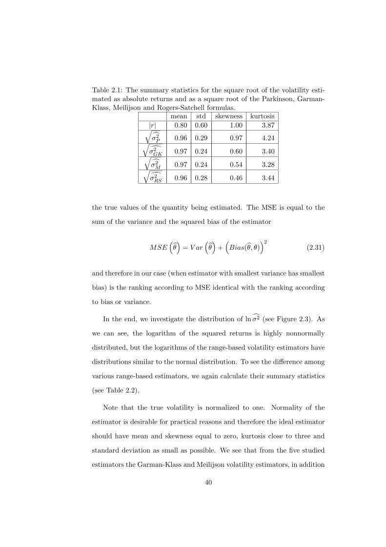
Table 2.1: The summary statistics for the square root of the volatility esti-mated as absolute returns and as a square root of the Parkinson, Garman-Klass, Meilijson and Rogers-Satchell formulas.
mean std skewness kurtosis
|r| 0.80 0.60 1.00 3.87√σ2P 0.96 0.29 0.97 4.24√σ2GK 0.97 0.24 0.60 3.40√σ2M 0.97 0.24 0.54 3.28√σ2RS 0.96 0.28 0.46 3.44
the true values of the quantity being estimated. The MSE is equal to the
sum of the variance and the squared bias of the estimator
MSE(θ)
= V ar(θ)
+(Bias(θ, θ)
)2(2.31)
and therefore in our case (when estimator with smallest variance has smallest
bias) is the ranking according to MSE identical with the ranking according
to bias or variance.
In the end, we investigate the distribution of ln σ2 (see Figure 2.3). As
we can see, the logarithm of the squared returns is highly nonnormally
distributed, but the logarithms of the range-based volatility estimators have
distributions similar to the normal distribution. To see the difference among
various range-based estimators, we again calculate their summary statistics
(see Table 2.2).
Note that the true volatility is normalized to one. Normality of the
estimator is desirable for practical reasons and therefore the ideal estimator
should have mean and skewness equal to zero, kurtosis close to three and
standard deviation as small as possible. We see that from the five studied
estimators the Garman-Klass and Meilijson volatility estimators, in addition
40
−4 −3 −2 −1 0 1 2 3 40
1
2x 10
4
squa
red
retu
rns
−4 −3 −2 −1 0 1 2 3 40
1
2x 10
4
Park
−4 −3 −2 −1 0 1 2 3 40
1
2x 10
4
GK
−4 −3 −2 −1 0 1 2 3 40
1
2x 10
4
M
−4 −3 −2 −1 0 1 2 3 40
2
4x 10
4
RS
Figure 2.3: Distribution of the logarithm of volatility estimated as squaredreturns and from the Parkinson, Garman-Klass, Meilijson and Rogers-Satchell formulas.
Table 2.2: Summary statistics for logarithm of volatility estimated as alogarithm of squared returns and as a logarithm of Parkinson, Garman-Klass, Meilijson and Rogers- Satchell volatility estimators.
mean std skewness kurtosis
ln(r2)
−1.27 2.22 −1.53 6.98
ln(σ2P
)−0.17 0.57 0.17 2.77
ln(σ2GK
)−0.13 0.51 −0.09 2.86
ln(σ2M
)−0.13 0.50 −0.14 2.86
ln(σ2RS
)−0.17 0.61 −0.71 5.41
41
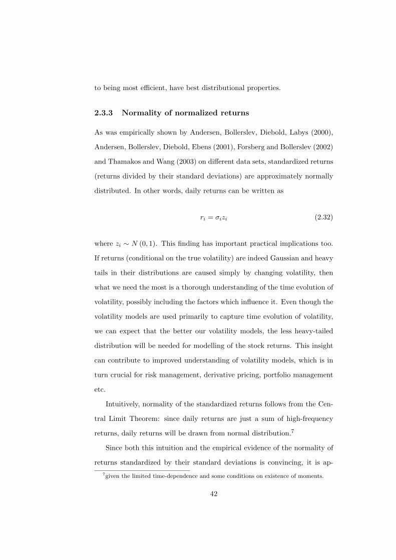
to being most efficient, have best distributional properties.
2.3.3 Normality of normalized returns
As was empirically shown by Andersen, Bollerslev, Diebold, Labys (2000),
Andersen, Bollerslev, Diebold, Ebens (2001), Forsberg and Bollerslev (2002)
and Thamakos and Wang (2003) on different data sets, standardized returns
(returns divided by their standard deviations) are approximately normally
distributed. In other words, daily returns can be written as
ri = σizi (2.32)
where zi ∼ N (0, 1). This finding has important practical implications too.
If returns (conditional on the true volatility) are indeed Gaussian and heavy
tails in their distributions are caused simply by changing volatility, then
what we need the most is a thorough understanding of the time evolution of
volatility, possibly including the factors which influence it. Even though the
volatility models are used primarily to capture time evolution of volatility,
we can expect that the better our volatility models, the less heavy-tailed
distribution will be needed for modelling of the stock returns. This insight
can contribute to improved understanding of volatility models, which is in
turn crucial for risk management, derivative pricing, portfolio management
etc.
Intuitively, normality of the standardized returns follows from the Cen-
tral Limit Theorem: since daily returns are just a sum of high-frequency
returns, daily returns will be drawn from normal distribution.7
Since both this intuition and the empirical evidence of the normality of
returns standardized by their standard deviations is convincing, it is ap-
7given the limited time-dependence and some conditions on existence of moments.
42
pealing to require that one of the properties of a ”good” volatility estima-
tor should be that returns standardized by standard deviations obtained
from this estimator will be normally distributed (see e.g. Bollen and In-
der (2002)). However, this intuition is not correct. As I now show, returns
standardized by some estimate of the true volatility do not need to, and gen-
erally will not, have the same properties as returns standardized by the true
volatility. Therefore we need to understand whether the range-based volatil-
ity estimators are suitable for standardization of the returns. There are two
problems associated with these volatility estimators: they are noisy and
their estimates might be (and typically are) correlated with returns. These
two problems might cause returns standardized by the estimated standard
deviations not to be normal, even when the returns standardized by their
true standard deviations are normally distributed.
Noise in volatility estimators
We want to know the effect of noise in volatility estimates σi on the dis-
tribution of returns normalized by these estimates (zi = ri/σi) when true
normalized returns zi = ri/σi are normally distributed. Without loss of
generality, we set σi = 1 and generate one million observations of ri, i ∈
{1, ..., 1000000}, all of them are iid N(0,1). Next we generate σi,n in such
a way that σ is unbiased estimator of σ, i.e. E (σi,n) = 1 and n repre-
sents the level of noise in σi,n. There is no noise for n = 0 and therefore
σi,0 = σi = 1. To generate σi,n for i > 0 we must decide upon distribution
of σi,n. Since we know from the previous section that range-based volatility
estimates are approximately lognormally distributed, we draw estimates of
the standard deviations from lognormal distributions. We set the parame-
ters µ and s2 of lognormal distribution in such a way that E (σi,n) = 1 and
43
Var(σi,n) = n, particularly µ = −12 ln (1 + n), s2 = ln (1 + n). For every n,
we generate one million observations of σi,n. Next we calculate normalized
returns zi,n = ri/σi,n. Their summary statistics is in the Table 2.3.
Table 2.3: Summary statistics for a random variable obtained as ratio ofnormal random variable with zero mean and variance one and lognormalrandom variable with constant mean equal to one and variance increasingfrom 0 to 0.8.n = V ar (σi) mean(zi,n) std(zi,n) skewness(zi,n) kurtosis(zi,n)
0.0 0.0001 1.00 0.00 3.00
0.2 0.0003 1.32 0.02 6.22
0.4 0.0013 1.66 −0.01 11.80
0.6 −0.0007 2.03 0.03 19.76
0.8 0.0025 2.43 0.01 34.60
Obviously, zi,0, which is by definition equal to ri, has zero mean, stan-
dard deviation equal to 1, skewness equal to 0 and kurtosis equal to 3. We
see that normalization by σ, a noisy estimate of σ, does not change E(z)
and skewness of z. This is natural, because ri is distributed symmetrically
around zero. On the other hand, adding noise increases standard devia-
tion and kurtosis of z. When we divide normally distributed random vari-
able ri by random variable σi, we are effectively adding noise to ri, making
its distribution flatter and more dispersed with more extreme observations.
Therefore, standard deviation increases. Since kurtosis is influenced mostly
by extreme observations, it increases too.
Bias introduced by normalization of range-based volatility estima-
tors
Previous analysis suggests that the more noisy volatility estimator we use for
the normalization of the returns, the higher the kurtosis of the normalized
returns will be. Therefore we could expect to find the highest kurtosis when
using the Parkinson volatility estimator (2.13). As we will see later, this is
44
−3 −2 −1 0 1 2 30
1
2x 10
4
true
−3 −2 −1 0 1 2 30
5000
10000
PA
RK
−3 −2 −1 0 1 2 3012
x 104
GK
−3 −2 −1 0 1 2 30
5000
10000
M
−3 −2 −1 0 1 2 3024
x 104
RS
Figure 2.4: Distribution of normalized returns. ”true” is the distribution ofthe stock returns normalized by the true standard deviations. This distribu-tion is by assumption N(0,1). PARK, GK, M and RS refer to distributionsof the same returns after normalization by volatility estimated using theParkinson, Garman-Klass, Meilijson and Rogers-Sanchell volatility estima-tors.
not the case. Returns and estimated standard deviations were independent
in the previous section, but this is not the case when we use range-based
estimators.
Let us denote σPARK ≡√σ2PARK , σGK ≡
√σ2RS , σM ≡
√σ2M and
σRS,t ≡√σ2RS . We study the distributions of zPARK,i ≡ ri/σPARK,i,
zGK,i ≡ ri/σGK,i, zM,i ≡ ri/σM,i, zRS,t ≡ ri/σRS,i. Histograms for these
distributions are shown in Figure 2.4 and corresponding summary statistics
are in Table 2.4.
The true mean and skewness of these distributions are zero, because re-
turns are symmetrically distributed around zero, triplets (h, l, c) and (−l,−h,−c)
are equally likely and all the studied estimators are symmetric in the sense
45
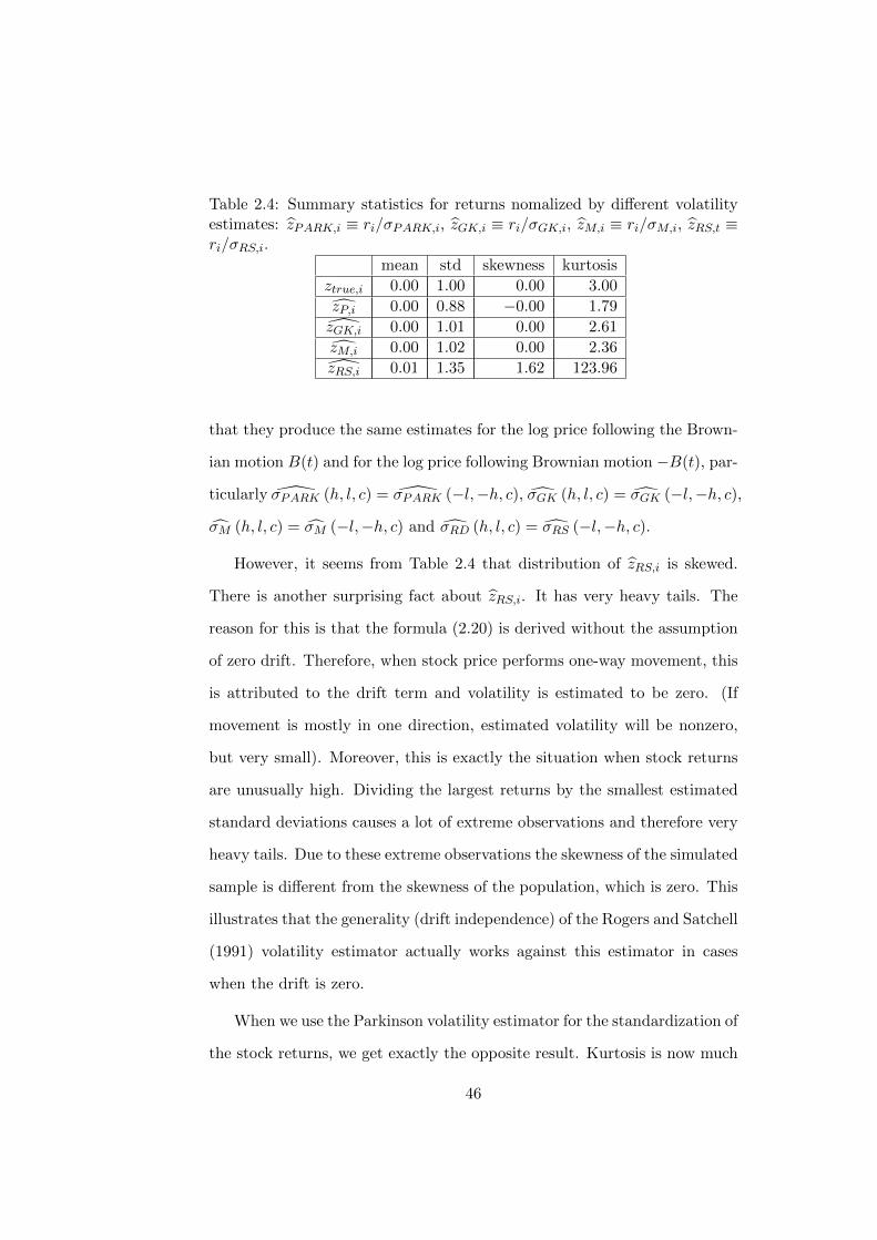
Table 2.4: Summary statistics for returns nomalized by different volatilityestimates: zPARK,i ≡ ri/σPARK,i, zGK,i ≡ ri/σGK,i, zM,i ≡ ri/σM,i, zRS,t ≡ri/σRS,i.
mean std skewness kurtosis
ztrue,i 0.00 1.00 0.00 3.00
zP,i 0.00 0.88 −0.00 1.79
zGK,i 0.00 1.01 0.00 2.61
zM,i 0.00 1.02 0.00 2.36
zRS,i 0.01 1.35 1.62 123.96
that they produce the same estimates for the log price following the Brown-
ian motion B(t) and for the log price following Brownian motion −B(t), par-
ticularly σPARK (h, l, c) = σPARK (−l,−h, c), σGK (h, l, c) = σGK (−l,−h, c),
σM (h, l, c) = σM (−l,−h, c) and σRD (h, l, c) = σRS (−l,−h, c).
However, it seems from Table 2.4 that distribution of zRS,i is skewed.
There is another surprising fact about zRS,i. It has very heavy tails. The
reason for this is that the formula (2.20) is derived without the assumption
of zero drift. Therefore, when stock price performs one-way movement, this
is attributed to the drift term and volatility is estimated to be zero. (If
movement is mostly in one direction, estimated volatility will be nonzero,
but very small). Moreover, this is exactly the situation when stock returns
are unusually high. Dividing the largest returns by the smallest estimated
standard deviations causes a lot of extreme observations and therefore very
heavy tails. Due to these extreme observations the skewness of the simulated
sample is different from the skewness of the population, which is zero. This
illustrates that the generality (drift independence) of the Rogers and Satchell
(1991) volatility estimator actually works against this estimator in cases
when the drift is zero.
When we use the Parkinson volatility estimator for the standardization of
the stock returns, we get exactly the opposite result. Kurtosis is now much
46
smaller than for the normal distribution. This is in line with empirical
finding of Bollen and Inder (2002). However, this result should not be
interpreted that this estimator is not working properly. Remember that we
got the result of the kurtosis being significantly smaller than 3 under ideal
conditions, when the Parkinson estimator works perfectly (in the sense that
it works exactly as it is supposed to work). Remember that this estimator is
based on the range. Even though the range, which is based on high and low
prices, seems to be independent of return, which is based on the open and
close prices, the opposite is the case. Always when return is high, range will
be relatively high too, because range is always at least as large as absolute
value of the return. |r| /σPARK will never be larger than√
4 ln 2, because
|r|σPARK
=|r|h−l√4 ln 2
=√
4 ln 2|r|h− l
≤√
4 ln 2 (2.33)
The correlation between |r| and σPARK is 0.79, what supports our argument.
Another problem is that the distribution of zP,i is bimodal.
As we can see from the histogram, distribution of zM,i does not have any
tails either. This is because the Meilijson volatility estimator suffers from
the same type of problem as the Parkinson volatility estimator, just to a
much smaller extent.
The Garman-Klass volatility estimator combines the Parkinson volatil-
ity estimator with simple squared return. Even though both, the Parkinson
estimator and squared return are highly correlated with size of the return,
the overall effect partially cancels out, because these two quantities are sub-
tracted. Correlation between |r| and σGK is indeed only 0.36. zGK,i has
approximately normal distribution, as the effect of noise and the effect of
correlation with returns to large extent cancels out.
47
We conclude this subsection with the appeal that we should be aware
of the assumptions behind the formulas we use. As range-based volatility
estimators were derived to be as precise volatility estimators as possible,
they work well for this purpose. However, there is no reason why all of these
estimators should work properly when used for the standardization of the
returns. We conclude that from the studied estimators the only estimator
appropriate for standardization of returns is the Garman-Klass volatility
estimator. We use this estimator later in the empirical part.
2.3.4 Jump component
So far in this paper, returns and volatilities were related to the trading day,
i.e. the period from the open to the close of the market. However, most
of the assets are not traded continuously for 24 hours a day. Therefore,
opening price is not necessarily equal to the closing price from the previous
day. We are interested in daily returns
ri = ln(Ci)− ln(Ci−1) (2.34)
simply because for the purposes of risk management we need to know the
total risk over the whole day, not just the risk of the trading part of the
day. If we do not adjust range-based estimators for the presence of opening
jumps, they will of course underestimate the true volatility. The Parkinson
volatility estimator adjusted for the presence of opening jumps is
σ2P =(h− l)2
4 ln 2+ j2 (2.35)
48
where ji = ln(Oi) − ln(Ci−1) is the opening jump. The jump-adjusted
Garman-Klass volatility estimator is:
σ2GK = 0.5 (h− l)2 − (2 ln 2− 1) c2 + j2 (2.36)
Other estimators should be adjusted in the same way. Unfortunately, includ-
ing opening jump will increase variance of the estimator when opening jumps
are significant part of daily returns.8 However, this is the only way how to
get unbiased estimator without imposing some additional assumptions. If
we knew what part of the overall daily volatility opening jumps account for,
we could find optimal weights for the jump volatility component and for
the volatility within the trading day to minimize the overall variance of the
composite estimator. This is done in Hansen and Lunde (2005), who study
how to combine opening jump and realized volatility estimated from high
frequency data into the most efficient estimator of the whole day volatility.
However, the relation of opening jump and the trading day volatility can
be obtained only from data. Moreover, there is no obvious reason why the
relationship from the past should hold in the future. Simply adding jump
component makes range-based estimators unbiased without imposing any
additional assumption.9
Adjustment for an opening jump is not as obvious as it seems to be and
even researchers quite often make mistakes when dealing with this issue.
The most common mistake is that the range-based volatility estimators are
not adjusted for the presence of opening jumps at all (see e.g. Parkinson
volatility estimator in Bollen, Inder (2002)). A less common mistake, but
with worse consequences is an incorrect adjustment for the opening jumps.
8Jump volatility is estimated with smaller precision than volatility within trading day.9These assumptions could be based on past data, but they would still be just assump-
tions.
49
E.g. Bollen and Inder (2002) and Fiess and MacDonald (2002) refer to the
following formula
σ2GKwrong,i = 0.5 (lnHi − lnLi)2 − (2 ln 2− 1) (lnCi − lnCi−1)
2 (2.37)
as Garman-Klass formula. This ”Garman-Klass volatility estimator” will
on average be even smaller than a Garman-Klass estimator not adjusted for
jumps. Moreover, it sometimes produces negative estimates for volatility
(variance σ2).
2.4 Normalized returns - empirics
Andersen, Bollerslev, Diebold, and Ebens (2001) find that ”although the
unconditional daily return distributions are leptokurtic, the daily returns
normalized by the realized standard deviations are close to normal.” Their
conclusion is based on standard deviations obtained these from high fre-
quency data. We study whether (and to what extend) this result is obtain-
able when standard deviations are estimated from daily data only.
We study stocks which were the components of the Dow Jow Industrial
Average on January 1, 2009, namely AA, AXP, BA, BAC, C, CAT, CVX,
DD, DIS, GE, GM, HD, HPQ, IBM, INTC, JNJ, JPM, CAG10, KO, MCD,
MMM, MRK, SFT, PFE, PG, T, UTX, VZ and WMT. We use daily open,
high, low and close prices. The data covers years 1992 to 2008. Stock prices
are adjusted for stock splits and similar events. We have 4171 daily obser-
vations for every stock. These data were obtained from the CRSP database.
We study DJI components to make our results as highly comparable as pos-
10Since historical data for KFT (component of DJI) are not available for the completeperiod, we use its biggest competitor CAG instead.
50

sible with the results of Andersen, Bollerslev, Diebold, and Ebens (2001).
For brevity, we study only two estimators: the Garman-Klass estima-
tor (2.15) and the Parkinson estimator (2.13). We use the Garman-Klass
volatility estimator because our previous analysis shows that it is the most
appropriate one. We use the Parkinson volatility estimator to demonstrate
that even though this estimator is the most commonly used range-based
estimator, it should not be used for normalization of returns. Moreover, we
study the effect of including or excluding a jump component into range-based
volatility estimators.
First of all, we need to distinguish the daily returns and the trading
day returns. By the daily returns we mean close-to-close returns, calcu-
lated according to formula (2.34). By the trading day returns we mean
returns during the trading hours, i.e. open-to-close returns, calculated ac-
cording to formula (2.2). We estimate volatilities accordingly: volatility of
the trading day returns from (2.13) and (2.15) and the volatility of the daily
returns using (2.35) and (2.36). Next we calculate standardized returns. We
calculate standardized returns in three different ways: trading day returns
standardized by trading day standard deviations (square root of trading
day volatility), daily returns standardized by daily standard deviation and
daily returns standardized by trading day standard deviation. Why do we
investigate daily returns standardized by trading day standard deviations
too? Theoretically, this does not make much sense because the return and
the standard deviations are related to different time intervals. However, it
is still quite common (see e.g. Andersen, Bollerslev, Diebold, and Ebens
(2001)), because people are typically interested in daily returns, but the
daily volatility cannot be estimated as precisely as trading day volatility.
The volatility of the trading part of the day can be estimated very precisely
51
from the high frequency data, whereas estimation of the daily volatility is
always less precise because of the necessity of including the opening jump
component. Therefore, trading day volatility is commonly used as a proxy
for daily volatility. This approximation is satisfactory as long as the opening
jump is small in comparison to trading day volatility, which is typically the
case.
Now we calculate summary statistics for the different standardized re-
turns as well as returns themselves. Results for the standard deviations are
presented in Table 2.5 and results for the kurtosis are presented in Table
2.6. We do not put similar tables for mean and kurtosis into this paper,
because these results are less interesting and can be summarized in one sen-
tance: Mean returns are always very close to zero, independent of which
standardization we used. Skewness is always very close to zero too.
The results for standard deviations and kurtosis are generally in line with
the predictions from our simulations too. First let us discuss the standard
deviations of the standardized returns. As Table 2.5 documents, normaliza-
tion by standard deviations obtained from the Parkinson volatility estimator
results in standard deviation smaller than one, approximately around 0.9
whereas normalization by standard deviation obtained from the Garman-
Klass volatility estimator results in standard deviations larger than one,
around 1.05. Normalization by standard deviations estimated from GARCH
model is approximately 1.1. This is expected as well, because division by a
noisy random variable increases the standard deviation.
Results for the kurtosis of standardized returns (see Table 2.6) are in
line with the predictions from our simulations too. Return distributions
have heavy tails (kurtosis significantly larger than 3). Second, the daily
returns normalized by the standard deviations calculated from Garman-
52
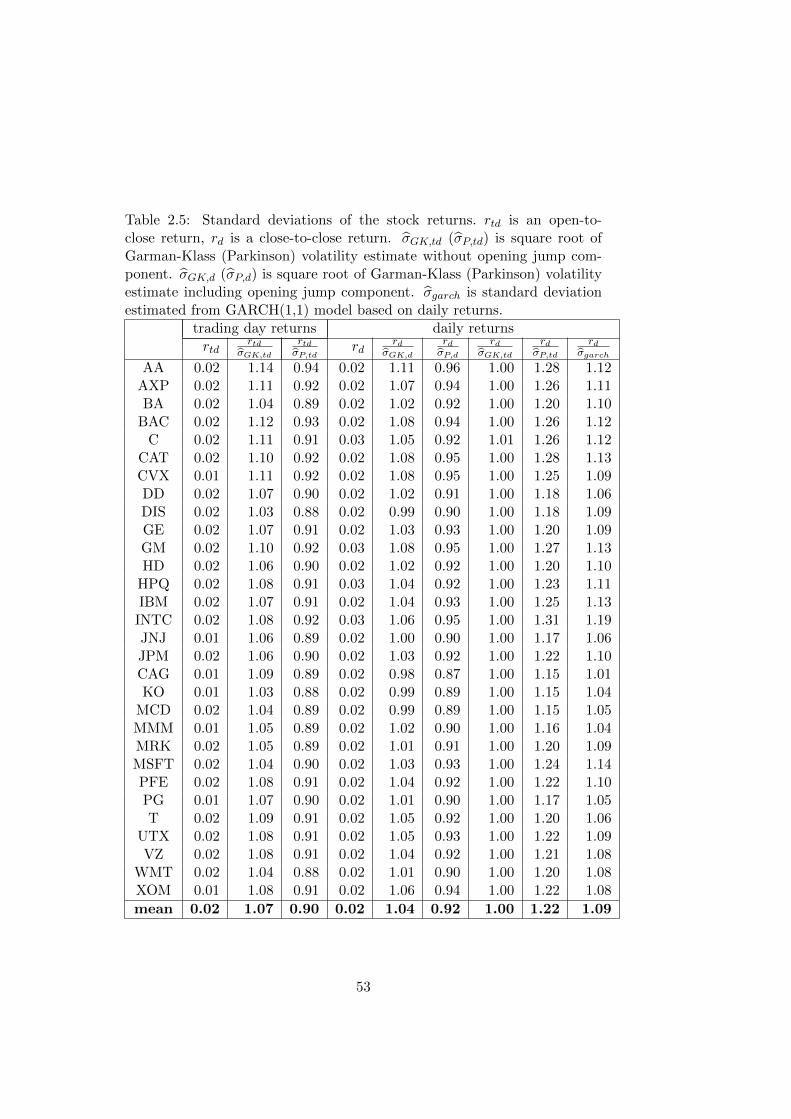
Table 2.5: Standard deviations of the stock returns. rtd is an open-to-close return, rd is a close-to-close return. σGK,td (σP,td) is square root ofGarman-Klass (Parkinson) volatility estimate without opening jump com-ponent. σGK,d (σP,d) is square root of Garman-Klass (Parkinson) volatilityestimate including opening jump component. σgarch is standard deviationestimated from GARCH(1,1) model based on daily returns.
trading day returns daily returnsrtd
rtdσGK,td
rtdσP,td
rdrd
σGK,drdσP,d
rdσGK,td
rdσP,td
rdσgarch
AA 0.02 1.14 0.94 0.02 1.11 0.96 1.00 1.28 1.12AXP 0.02 1.11 0.92 0.02 1.07 0.94 1.00 1.26 1.11BA 0.02 1.04 0.89 0.02 1.02 0.92 1.00 1.20 1.10
BAC 0.02 1.12 0.93 0.02 1.08 0.94 1.00 1.26 1.12C 0.02 1.11 0.91 0.03 1.05 0.92 1.01 1.26 1.12
CAT 0.02 1.10 0.92 0.02 1.08 0.95 1.00 1.28 1.13CVX 0.01 1.11 0.92 0.02 1.08 0.95 1.00 1.25 1.09DD 0.02 1.07 0.90 0.02 1.02 0.91 1.00 1.18 1.06DIS 0.02 1.03 0.88 0.02 0.99 0.90 1.00 1.18 1.09GE 0.02 1.07 0.91 0.02 1.03 0.93 1.00 1.20 1.09GM 0.02 1.10 0.92 0.03 1.08 0.95 1.00 1.27 1.13HD 0.02 1.06 0.90 0.02 1.02 0.92 1.00 1.20 1.10
HPQ 0.02 1.08 0.91 0.03 1.04 0.92 1.00 1.23 1.11IBM 0.02 1.07 0.91 0.02 1.04 0.93 1.00 1.25 1.13
INTC 0.02 1.08 0.92 0.03 1.06 0.95 1.00 1.31 1.19JNJ 0.01 1.06 0.89 0.02 1.00 0.90 1.00 1.17 1.06JPM 0.02 1.06 0.90 0.02 1.03 0.92 1.00 1.22 1.10CAG 0.01 1.09 0.89 0.02 0.98 0.87 1.00 1.15 1.01KO 0.01 1.03 0.88 0.02 0.99 0.89 1.00 1.15 1.04
MCD 0.02 1.04 0.89 0.02 0.99 0.89 1.00 1.15 1.05MMM 0.01 1.05 0.89 0.02 1.02 0.90 1.00 1.16 1.04MRK 0.02 1.05 0.89 0.02 1.01 0.91 1.00 1.20 1.09MSFT 0.02 1.04 0.90 0.02 1.03 0.93 1.00 1.24 1.14PFE 0.02 1.08 0.91 0.02 1.04 0.92 1.00 1.22 1.10PG 0.01 1.07 0.90 0.02 1.01 0.90 1.00 1.17 1.05T 0.02 1.09 0.91 0.02 1.05 0.92 1.00 1.20 1.06
UTX 0.02 1.08 0.91 0.02 1.05 0.93 1.00 1.22 1.09VZ 0.02 1.08 0.91 0.02 1.04 0.92 1.00 1.21 1.08
WMT 0.02 1.04 0.88 0.02 1.01 0.90 1.00 1.20 1.08XOM 0.01 1.08 0.91 0.02 1.06 0.94 1.00 1.22 1.08
mean 0.02 1.07 0.90 0.02 1.04 0.92 1.00 1.22 1.09
53
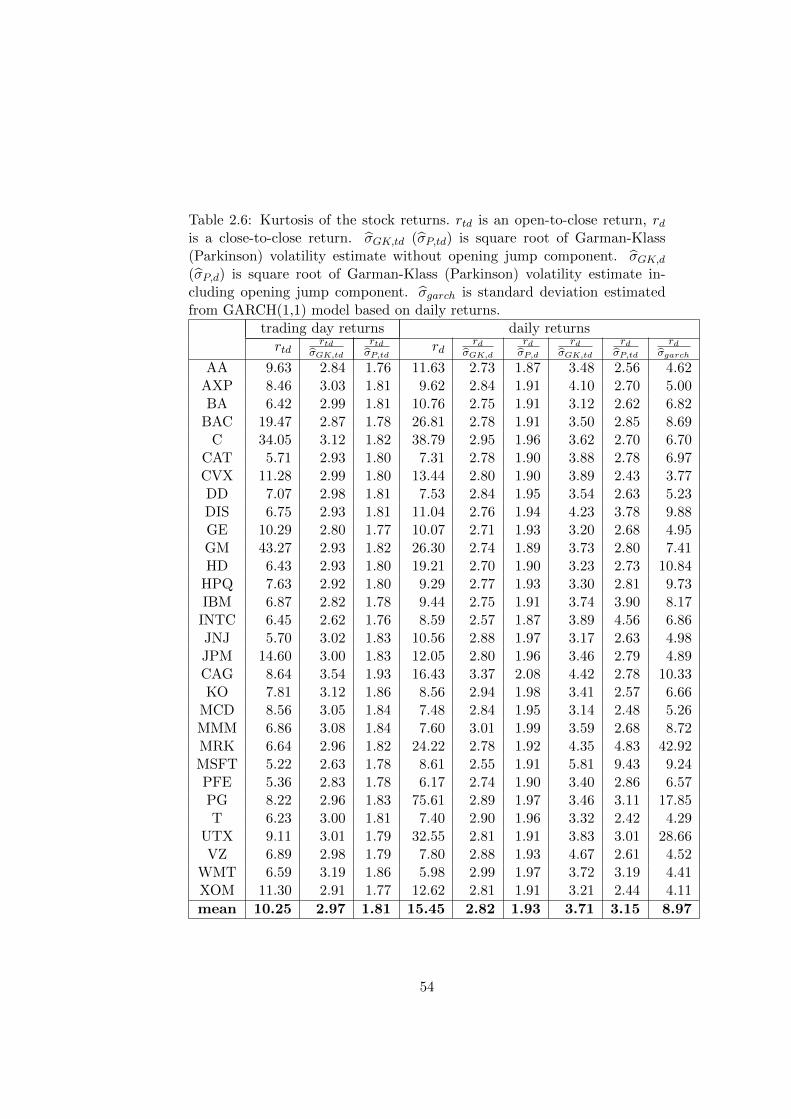
Table 2.6: Kurtosis of the stock returns. rtd is an open-to-close return, rdis a close-to-close return. σGK,td (σP,td) is square root of Garman-Klass(Parkinson) volatility estimate without opening jump component. σGK,d(σP,d) is square root of Garman-Klass (Parkinson) volatility estimate in-cluding opening jump component. σgarch is standard deviation estimatedfrom GARCH(1,1) model based on daily returns.
trading day returns daily returnsrtd
rtdσGK,td
rtdσP,td
rdrd
σGK,drdσP,d
rdσGK,td
rdσP,td
rdσgarch
AA 9.63 2.84 1.76 11.63 2.73 1.87 3.48 2.56 4.62AXP 8.46 3.03 1.81 9.62 2.84 1.91 4.10 2.70 5.00BA 6.42 2.99 1.81 10.76 2.75 1.91 3.12 2.62 6.82
BAC 19.47 2.87 1.78 26.81 2.78 1.91 3.50 2.85 8.69C 34.05 3.12 1.82 38.79 2.95 1.96 3.62 2.70 6.70
CAT 5.71 2.93 1.80 7.31 2.78 1.90 3.88 2.78 6.97CVX 11.28 2.99 1.80 13.44 2.80 1.90 3.89 2.43 3.77DD 7.07 2.98 1.81 7.53 2.84 1.95 3.54 2.63 5.23DIS 6.75 2.93 1.81 11.04 2.76 1.94 4.23 3.78 9.88GE 10.29 2.80 1.77 10.07 2.71 1.93 3.20 2.68 4.95GM 43.27 2.93 1.82 26.30 2.74 1.89 3.73 2.80 7.41HD 6.43 2.93 1.80 19.21 2.70 1.90 3.23 2.73 10.84
HPQ 7.63 2.92 1.80 9.29 2.77 1.93 3.30 2.81 9.73IBM 6.87 2.82 1.78 9.44 2.75 1.91 3.74 3.90 8.17
INTC 6.45 2.62 1.76 8.59 2.57 1.87 3.89 4.56 6.86JNJ 5.70 3.02 1.83 10.56 2.88 1.97 3.17 2.63 4.98JPM 14.60 3.00 1.83 12.05 2.80 1.96 3.46 2.79 4.89CAG 8.64 3.54 1.93 16.43 3.37 2.08 4.42 2.78 10.33KO 7.81 3.12 1.86 8.56 2.94 1.98 3.41 2.57 6.66
MCD 8.56 3.05 1.84 7.48 2.84 1.95 3.14 2.48 5.26MMM 6.86 3.08 1.84 7.60 3.01 1.99 3.59 2.68 8.72MRK 6.64 2.96 1.82 24.22 2.78 1.92 4.35 4.83 42.92MSFT 5.22 2.63 1.78 8.61 2.55 1.91 5.81 9.43 9.24PFE 5.36 2.83 1.78 6.17 2.74 1.90 3.40 2.86 6.57PG 8.22 2.96 1.83 75.61 2.89 1.97 3.46 3.11 17.85T 6.23 3.00 1.81 7.40 2.90 1.96 3.32 2.42 4.29
UTX 9.11 3.01 1.79 32.55 2.81 1.91 3.83 3.01 28.66VZ 6.89 2.98 1.79 7.80 2.88 1.93 4.67 2.61 4.52
WMT 6.59 3.19 1.86 5.98 2.99 1.97 3.72 3.19 4.41XOM 11.30 2.91 1.77 12.62 2.81 1.91 3.21 2.44 4.11
mean 10.25 2.97 1.81 15.45 2.82 1.93 3.71 3.15 8.97
54
Klass formula are close to normal (kurtosis is close to 3). Third, the daily
returns normalized by the standard deviations calculated from Parkinson
formula have no tails (kurtosis is significantly smaller than 3). Fourth,
normalization of daily returns by standard deviation estimated for trading
day only, will cause upward bias in kurtosis. This is a consequence of the
standardization by an incorrect standard deviation - sometimes (particularly
in a situation when the opening jump is large), returns are divided by too
small standard deviation, which will cause too many large observations for
normalized returns.
The last column of Table 2.6 reports kurtosis of returns normalized by
standard deviations estimated from GARCH(1,1) model with mean return
fixed to zero. As we can see, these normalized returns are not Gaussian, they
have fat tails. This is consistent with the fact that GARCH models with fat-
tailed conditional distribution of returns fit data better than GARCH models
with conditionally normally distributed returns. However, as is clear from
this paper, this is the case simply because GARCH models always condition
return distribution on the estimated volatility, which is only a noisy proxy of
the true volatility. Therefore, even when distribution of returns conditional
on the true volatility is Gaussian, distribution of returns conditional on
estimated volatility will have heavy tails. This result has an important
implication for volatility modelling: the more precisely we can estimate the
volatility, the closer will be the conditional distribution of returns to the
normal distribution.
2.5 Conclusion
Range-based volatility estimators provide significant increase in accuracy
compared to simple squared returns. Even though efficiency of these esti-
55
mators is known, there is some confusion about other properties of these
estimators. We study these properties. Our main focus is the properties of
returns standardized by their standard deviations.
First, we correct some mistakes in existing literature. Second, we study
different properties of range-based volatility estimators and find that for
most purposes, the best volatility estimators is the Garman-Klass volatility
estimator. The Meilijson volatility estimator improves its efficiency slightly,
but it is based on a significantly more complicated formula. However, per-
formance of all the range-based volatility estimators is similar in most cases
except for the case when we want to use them for standardization of the
returns.
Returns standardized by their standard deviations are known to be nor-
mally distributed. This fact is important for the volatility modelling. This
result was possible to obtain only when the standard deviations were esti-
mated from the high frequency data. When the standard deviations were
obtained from volatility models based on daily data, returns standardized by
these standard deviations are not Gaussian anymore, they have heavy tails.
Using simulations we show that even when returns themselves are normally
distributed, returns standardized by (imprecisely) estimated volatility are
not normally distributed; their distribution has heavy tails. In other words:
the fact that standard volatility models show that even conditional distribu-
tion of returns has heavy tails does not mean that returns are not normally
distributed. It means that these models cannot estimate volatility precisely
enough and the noise in the volatility estimates causes the heavy tails.
It is not obvious whether range-based volatility estimators can be used
for the standardization of the returns. Using simulations we find that for
the purpose of returns standardization there are large differences between
56

these estimators and we find that the Garman-Klass volatility estimator is
the only one appropriate for this purpose. Putting all the results together,
we rate the Garman-Klass volatility estimator as the best volatility estima-
tor based on daily (open, high, low and close) data. We test this estimator
empirically and we find that we can indeed obtain basically the same results
from daily data as Andersen, Bollerslev, Diebold, and Ebens (2001) ob-
tained from high-frequency (transaction) data. This is important, because
the high-frequency data are very often not available or available only for a
shorter time period and their processing is complicated. Since returns scaled
by standard deviations estimated from GARCH type of models (based on
daily returns) are not Gaussian (they have fat tails), our results show that
the GARCH type of models cannot capture the volatility precisely enough.
Therefore, in the absence of high-frequency data, further development of
volatility models based on open, high, low and close prices is recommended.
57

58
Bibliography
[1] Alizadeh, S., Brandt, M. W., & Diebold, F. X. (2002). Range-based
estimation of stochastic volatility models. Journal of Finance, 57, 1047–
1091.
[2] Andersen T. G., Bollerslev T., Diebold F.X., & Labys, P. (2000). Ex-
change rate returns standardized by realized volatility are nearly Gaus-
sian. Multinational Finance Journal, 4, 159–179.
[3] Andersen, T. G., Bollerslev, T. Diebold F.X. & Ebens, H. (2001). The
distribution of realized stock return volatility. Journal of Financial Eco-
nomics, 61, 43–76.
[4] Bali, T. G., & Weinbaum, D. (2005). A comparative study of alter-
native extreme-value volatility estimators. Journal of Futures Markets,
25, 873–892.
[5] Bernard Bollen, B., & Inder, B. (2002). Estimating daily volatility in
financial markets, Journal of Empirical Finance, 9, 551–562.
[6] Brandt, M. W., & Diebold, F. X. 2006. A no-arbitrage approach to
range based estimation of return covariances and correlations. Journal
of Business, 79, 61–74.
59
[7] Brandt, M. W., & Jones., Ch. S. (2006). Volatility forecasting with
Range-Based EGARCH models. Journal of Business and Economic
Statistics, 24 (4), 470–486.
[8] Broto, C. & Ruiz, E. (2004), Estimation methods for stochastic volatil-
ity models: a survey. Journal of Economic Surveys, 18, 613–649.
[9] Chou, R. Y. (2005) Forecasting financial volatilities with extreme val-
ues: the conditional autoregressive range (CARR) model. Journal of
Money, Credit and Banking, 37 (3), 561–582.
[10] Chou, R. Y., 2006. Modeling the asymmetry of stock movements using
price ranges. Advances in Econometrics, 20, 231–258.
[11] Chou, R. Y., Chou, H., & Liu, N. (2010). Range volatility models and
their applications in finance. Handbook of Quantitative Finance and
Risk Management, Chapter 83, Springer.
[12] Chou, R. Y., & Liu, N. (2010). The economic value of volatility timing
using a range-based volatility model. Journal of Economic Dynamics &
Control, 34, 2288–2301.
[13] Dacorogna, M. M., Gencay, R., Muller, U. A., Olsen, R. B., & Pictet,
O. V. (2001). An Introduction to High-Frequency Finance. San Diego:
Academic Press.
[14] Feller, W. (1951). The asymptotic distribution of the range of sums of
independent random variables. The Annals of Mathematical Statistics,
22, 427–432.
[15] Fiess, N. M., & MacDonald, R. (2002). Towards the fundamentals of
technical analysis: analysing the information content of High, Low and
Close proces. Economic Modelling, 19, 354–374.
60
[16] Forsberg, L., & Bollerslev, T. (2002). Bridging the gap between the
distribution of realized (ECU) volatility and ARCH modelling (of the
Euro): the GARCH-NIG model. Journal of Applied Econometrics, 17,
535–548.
[17] Garman, M. B., & Klass, M. J. (1980). On the Estimation of Security
Price Volatilities from Historical Data. The Journal of Business, 53 (1),
67–7
[18] Hansen, P. R., & Lunde, A. (2005). A realized variance for the whole
day based on intermittent high-frequency data. Journal of Financial
Econometrics, 3, 525–554.
[19] Karatzas, I., & Shreve, S. E. (1991). Brownian Motion and Stochastic
Calculus. New York: Springer-Verlag.
[20] Kunitomo, N. (1992). Improving the Parkinson method of estimating
security price volatilities. Journal of Business, 65, 295–302.
[21] Meilijson, I., (2009), The Garman–Klass volatil-
ity estimator revisited, working paper available at:
http://arxiv.org/PS cache/arxiv/pdf/0807/0807.3492v2.pdf
[22] Parkinson, M. (1980). The extreme value method for estimating the
variance of the rate of return. Journal of Business, 53, 61–65.
[23] Rogers, L. C. G., & Satchell, S. E. (1991). Estimating variance from
high, low and closing prices. Annals of Applied Probability, 1, 504–12.
[24] Thomakos, D. D., Wang, T., (2003), Realized volatility in the futures
markets. Journal of Empirical Finance, 10, 321–353.
61

[25] Yang, D., & Zhang, Q. (2000). Drift-independent volatility estimation
based on high, low, open, and close prices. Journal of Business, 73,
477–491.
62

3Rethinking the GARCH
63
Abstract
Based on the view that GARCH volatility models should not be considered
as data-generating processes for volatility but as filters we suggest a simple
and general way to improve them using high and low prices. We illustrate
this on the GARCH(1,1) model and empirical analysis confirms our idea.
A modified GARCH(1,1) model performs significantly better than the stan-
dard GARCH(1,1) model regarding both in-sample fit and out-of-sample
forecasting ability.
Key words: volatility, GARCH, range, high, low 1
1I would like to thank to Jonas Andersson, Stein Erik Fleten, Milan Basta, LukasLaffers and participants at NHH and NTNU seminars for helpful comments.
64

3.1 Introduction
The most fundamental variables of finance and economics are changes of
asset prices (returns) and their variances. As was observed a long time
ago, even though returns of most financial assets are to a large extent un-
predictable, their variances display high temporal dependency and are pre-
dictable. Starting with the work of Engle (1982) and Bollerslev (1986), the
ARCH and GARCH classes of models have become such standard tools to
for volatility estimation and prediction that they can be found in many
undergraduate time series textbooks. Some of the widely used extensions
are EGARCH of Nelson (1991), GJR-GARCH of Glosten, Jagannathan and
Runkle (1993), FIEGARCH of Bollerslev and Mikkelsen (1996) and many
others. See e.g. Andersen et al. (2006) and Engle and Patton (2001) for
surveys and further references.
Starting with the work of Taylor (1986), a new class of volatility models
emerged - stochastic volatility models. For an overview see e.g. Ghysels
et al. (1996) and Shepard (1996). Since stochastic volatility models are
naturally formulated in continuous time, they are strongly connected with
standard continuous time finance. They proved to be useful particularly in
option pricing (see Hull and White (1987), Melino and Turnbull (1990)). The
direct comparison with GARCH type of models is inconclusive (Kim et al.
(1998)). The main reason why stochastic volatility models did not become as
popular as GARCH models is the practical one - stochastic volatility models
are much more difficult to estimate (see e.g. Broto and Ruiz (2004)).
The main difference between stochastic volatility and GARCH models
is the following. Stochastic volatility models assume that volatility evolves
over time as some stochastic proces and returns are drawn from a distribu-
tion parametrized by this volatility. Past returns have no direct effect on
65
the future volatility.2 In GARCH models, returns are generated the same
way as in the stochastic volatility models. The only stochastic element in
the volatility equation are past returns and therefore past returns determine
future volatility. In other words, returns are stochastic, but once the re-
turn was realized, future volatility is determined. If we consider GARCH
models and stochastic volatility models as data generating processes, they
are obviously mutually exclusive. However, important insight from Nelson
(1990, 1992) tells us that even when a GARCH model is misspecified (it is
not a true data generating process for the volatility), it can work quite well.
We can think of the GARCH model as a filter through which we pass the
data to produce an estimate of the conditional volatility. In his own words
(Nelson and Foster 1994):
”Likely reason for the empirical success of ARCH: when both observable
variables and conditional variances change ”slowly” relative to the sampling
interval (in particular, when the data generating process is well approxi-
mated by a diffusion and the data are observed at high frequencies) then
broad classes of ARCH models, even when misspecified, provide continuous-
record consistent estimates of the conditional variances. That is, as the
observable variables are recorded at finer and finer intervals, the conditional
variance estimates produced by the (misspecified) ARCH model converge in
probability to the true conditional variances.”
Our work is based on a similar intuition. The GARCH model can fit the
data quite well even when the volatility itself is not generated by the process
specified by the GARCH model. In GARCH type of models, demeaned3
2Abstracting from leverage effect, which can be possibly incorporated into the stochas-tic volatility models.
3For most of the assets, mean daily return is much smaller than its standard deviationand therefore can be considered equal to zero. From now on we assume that it is indeedzero. This assumption not only makes further analysis simpler, but it actually helpsto estimate volatility more precisely. In the words of Poon and Granger (2003): ”The
66
squared returns serve as a way to calculate an innovation to the volatility.
Rewriting GARCH models in terms of observed variables (returns) only
shows that the GARCH model in fact calculates volatility as a weighted
moving average of past squared returns. If volatility is changing slowly
over the time, the GARCH model will work simply because squared returns
are daily volatility estimates and the GARCH model essentially calculates
volatility as some kind of weighted moving average of the past volatilities.
This intuition has interesting implications. Most importantly, replace-
ment of the squared returns by more precise volatility estimates will produce
better GARCH models, both in terms of in-sample fit and out-of-sample
forecasting performance. Additionally, coefficients of GARCH models based
on more precise volatility estimates than squared returns will be changed in
such a way that they will put more weight on more recent observations. We
test both these implications.
To test our idea, we estimate a GARCH(1,1) model using both squared
returns and a more precise volatility proxy, in particular the Parkinson
(1980) volatility estimator based on range (the difference between high and
low). The results confirm our expectations.
In this way our work becomes closely related to Alizadeh, Brandt, Diebold
(2002), Chou (2005), Brandt and Jones (2006) who use range-based volatil-
ity measures to estimate volatility models. Alizadeh et al. (2002) estimate
a stochastic volatility model. Brandt and Jones (2006) estimate EGARCH
and FIEGARCH models based on log range. Chou (2005) uses range in
standard deviation GARCH. These papers employ range-based volatility
proxies in different volatility models. However, standard GARCH models
statistical properties of sample mean make it a very inaccurate estimate of the true mean,especially for small samples, taking deviations around zero instead of the sample meantypically increases volatility forecast accuracy.”
67
are estimated to fit the conditional distribution of returns, whereas previ-
ously mentioned models are estimated to fit the conditional distribution of
range (log-range). This in turn means that only our model can be estimated
using standard econometric software without any programming.
Our contribution is threefold. First, we construct a range-based GARCH
model (RGARCH), which is a simple modification of the standard widely
used GARCH(1,1) model, but still outperforms it significantly. Second, our
paper should be viewed as an illustration of how the existing GARCH mod-
els can be easily improved by using more precise volatility proxies. Even
though this paper devotes most of the space to illustrate that the RGARCH
models outperforms the standard GARCH(1,1) model, our main goal is not
to convince the reader that our model is the best one. On the contrary, since
leverage effect is a well-documented phenomenon, the asymmetric RGARCH
model is very likely to outperform our model. We leave this to further re-
search. Third, we confirm that GARCH models should indeed be considered
just filtering devices, not data generating processes.
The rest of the paper is organized in the following way: Section 2 pro-
vides a basic introduction to volatility modelling and an overview of existing
range-based volatility estimators. Section 3 decribes the data, methodology
and results. Finally, Section 4 concludes.
3.2 Theoretical background
3.2.1 GARCH models
Let Pt be the price of a speculative asset at the end of day t. Define return
rt as
rt = log (Pt)− log (Pt−1) (3.1)
68
Daily returns are known to be basically unpredictable and their expected
value is very close to zero. On the other hand, variance of daily returns
changes significantly over time. We assume that daily returns are drawn
from normal distribution with a zero mean and time-varying variance
rt ∼ N(0, σ2t
)(3.2)
Both assumptions, zero mean and normal distribution, are not necessary
and can be abandoned without any difficulty. For the sake of exposition,
we maintain these assumptions throughout the whole paper. This allows
us to focus on the modelling of conditional variance (volatility) only. The
first model to capture the time variation of volatility is Engle’s (1982) Auto
Regressive Conditional Heteroskedasticity (ARCH) model. The ARCH(p)
has the form:
σ2t = ω +
p∑i=1
αir2t−i (3.3)
where rt is a return in day t, σ2t is an estimate of the volatility in day t and ω
and αi’s are positive constants.The Generalized ARCH model was afterwards
introduced by Bollerslev (1986). The GARCH(p,q) has the following form:
σ2t = ω +
p∑i=1
αir2t−i +
q∑j=1
βiσ2t−j (3.4)
where the βi’s are positive constants. The GARCH model has become more
popular, because with just a few parameters it can fit data better than
a more parametrized ARCH model. Particularly popular is its simplest
69
version, the GARCH(1,1) model4:
σ2t = ω + αr2t−1 + βσ2t−1 (3.5)
Estimation of the GARCH(1,1) typically yields the following results. ω
is very small (e.g. 0.0006), α + β is close to one, but smaller than one.
Moreover, most of the weight is on the β coefficient, e.g. α = 0.04, β = 0.95.
In other words, the estimated GARCH(1,1) model is usually very close to its
reduced form, the Exponential Weighted Moving Average (EMWA) model
σ2t = αr2t−1 + (1− α)σ2t−1 (3.6)
The EMWA mode has one obvious disadvantage: time series of volatility
generated by the process (3.6) would not be stationary, whereas observed
volatility time series are stationary. However, this is not a problem if we
consider EMWA just as a filtering device. EMWA model is useful particu-
larly for didactic purposes. In this model the new volatility estimate is esti-
mated as a weighted average of the most recently observed volatility proxy
(squared returns) and the last estimate of the volatility. Loosely speaking,
we gradually update our belief about the volatility as new information (noisy
volatility proxy) becomes available. If the new information indicates that
the volatility was larger than our previous belief about it, we update our
belief upwards and vice versa. The coefficient α tells us how much weight
we put on the new information. If we use less noisy volatility proxy instead
of squared returns, optimal α should be larger and the performance of the
model should be better.
4Even though the GARCH(1,1) is a very simple model, it still works surprisingly wellin comparison with much more complex volatility models (see Hansen and Lunde (2005)).
70
The same intuition applies to GARCH models too. This naturally leads
to the proposal of the modified GARCH(1,1)
σ2t = ω + α σ2proxy,t−1 + βσ2t−1 (3.7)
where σ2proxy,t−1 is the less noisy volatility proxy.
Next we need to decide upon what should be used as a better (less
noisy) volatility proxy. Generally, the better the proxy we use, the better
should the model work. Therefore, the natural candidate would be realized
volatility. This would lead to models related to Shephard and Shephard
(2009). However, despite the atractiveness of the realized variance we do
not use it as a volatility proxy. Realized variance must be calculated from
high frequency data and these data are in many cases not available at all
or available only over shorter time horizons and costly to obtain and work
with. Moreover, due to market microstructure effects the volatility esti-
mation from high frequency data is a rather complex issue (see Dacorogna
et al. (2001)). Contrary to high frequency data, high (H) and low (L)
prices, which are usually widely available, can be used to estimate volatility
(Parkinson (1980)):
σ2P =[ln(H/L)]2
4 ln 2(3.8)
This estimator is based on the assumption that, during the day, the loga-
rithm of the price follows a Brownian motion with a zero drift. This assump-
tion typically holds quite well in the data. Parkinson’s volatility estimator is
the most used volatility estimator (see e.g. Alizadeh, Brandt, Diebold (2002)
or Brandt and Jones (2006)). An alternative volatility proxy we could use
is Garman-Klass (1980) volatility estimator, which utilizes additional open
71
(O) and close (C) data:
σ2GK = 0.5 [ln(H/L)]2 − (2 ln 2− 1) [ln(C/O)]2 (3.9)
Under ideal conditiona (Brownian motion with zero drift) this estimator is
less noisy than the Parkinson volatility estimator5, because it utilizes open
and close prices too. However, in this paper we use Parkinson’s volatility
estimator (σ2proxy = σ2P ). We have done all the calculations for the Garman-
Klass volatility estimator too and found out that for this particular purpose
usage of Garman-Klass estimator does not improve the results, the results
are practically the same as for the Parkinson volatility estimator. Moreover,
for the same data sets where high and low prices are available, open price is
sometimes not available.
In this paper we therefore study the following model
σ2t = ω + ασ2P,t−1 + βσ2t−1 (3.10)
which we denote as RGARCH(1,1) (range GARCH) model. This model can
obviously be extended to the RGARCH(p,q) model
σ2t = ω +
p∑i=1
αiσ2P,t−i +
q∑j=1
βiσ2t−j (3.11)
Since it is generally known that GARCH(p,q) of order higher than (1,1) is
seldom useful, we study the RGARCH model only in its simplest version
(3.10), i.e. the RGARCH(1,1) model. Most of the paper is devoted to the
comparison of the standard GARCH(1,1) model (3.5) and the RGARCH(1,1)
model (3.10). Since we do not study GARCH and RGARCH models of
5For comparison of range-based volatility estimators see Molnar (2011).
72

higher orders, we sometimes refer to GARCH(1,1) and RGACH(1,1) models
simply as GARCH and RGARCH models.
Our hypotheses are the following:
Hypothesis 1
RGARCH(1,1) outperforms the standard GARCH(1,1) model, both in sense
of the in sample fit and out of sample forecasting performance.
Additionaly, as previously explained, we expect that the estimated coef-
ficients of the GARCH models will be changed in such a way that more
weight will be put on the recent observation(s) of the volatility proxy. This
leads us to the second hypothesis.
Hypothesis 2
If we modify GARCH(1,1) to the RGARCH(1,1) model, we expect α to in-
crease and β to decrease.
To test hypothesis 1, we compare the modified GARCH(1,1) model (3.7)
not only with GARCH(1,1) model (3.5), but with other GARCH models
commonly used. Models we compare to our RGARCH are the following
ones:
The GJR-GARCH of Glosten, Jaganathan and Runkle (1993):
σ2t = ω + αr2t−1 + βσ2t−1 + γr2t−1It−1 (3.12)
where It = 1 if rt < 0 and zero otherwise,
73
The Exponantial GARCH (EGARCH) of Nelson (1991):
log(σ2t)
= ω + α
∣∣∣∣ rt−1σt−1
∣∣∣∣+ β log(σ2t−1
)+ γ
rt−1σt−1
(3.13)
The standard deviation GARCH of Taylor (1986) and Schwert (1989),
denoted in this paper as stdG, both in its symmetric version:
σt = ω + αrt−1 + βσt−1 (3.14)
and in the asymmetric version, similar to (3.12), taking into account the
leverage effect (astdG):
σt = ω + αrt−1 + βσt−1 + γrt−1It−1 (3.15)
The last model we use is the component GARCH (cGARCH).
σ2t −mt = ω + α(r2t−1 −mt
)+ β
(σ2t−1 −mt
)(3.16)
mt = ω + ρ (mt − ω) + φ(r2t−1 − σ2t−1
)(3.17)
The intuition for the component GARCH is the following. The standard
GARCH(1,1) model, which can be rewritten as
σ2t = ω + α(r2t−1 − ω
)+ β
(σ2t−1 − ω
)(3.18)
exhibits mean reversion around ω, which is constant. The component GARCH
allows mean reversion around the time varying level mt.
74
3.2.2 Estimation
All the GARCH models, including the models (3.5), (3.12) - (3.15) in our
paper are estimated via Maximum Likelihood. Since the RGARCH model
changes only the specification of the variance equation (equation (3.10) in-
stead of (3.10)), we do not need to derive new likelihood function for esti-
mation of this model. This in turns mean that our model can be estimated
without any programming in widely available econometric packages which
allow to include exogeneous variables in the variance equation, e.g. Eviews,
R or OxMetrics. We simply specify that we want to estimate GARCH(0,1)
model with exogeneous variable σ2P,t−1.
As mentioned earlier, we assume returns to be normally distributed
with zero mean (equation (3.2)) and variance evolving according to a given
GARCH model. However, there are alternative distributions for residuals
to consider (e.g. Student’s t-distribution, GED distribution,...). We did the
calculations for alternative distributions too, but we found that comparison
of the standard GARCH model vs. RGARCH model is unaffected by the
assumption of the residuals’ distribution as long as the return distribution
is the same for both models. For the sake of brevity, we report only the
results for the GARCH models with normally distributed residuals.
Two most closely related models are The Conditional Autoregressive
Range model (CARR) of Chou (2005) and Range-Based EGARCH model
(REGARCH) of Brandt and Jones (2006). Common feature of these mod-
els with the standard GARCH models is the variance equation. The vari-
ance equation for RGARCH model is created by modification of GARCH
(3.5), the variance equation of the CARR model is modification of GJR-
GARCH (3.12) and the variance equation of REGARCH is a modification
of EGARCH (3.13).
75
However, CARR and REGARCH are otherwise significantly different
from RGARCH and other GARCH models. Standard GARCH models as
well as RGARCH model are estimated by fitting the conditional distribution
of returns (equation(3.2). On contrary, estimation of the CARR and the
REGARCH models is based on range. Denote
Dt = ln (Ht/Lt) (3.19)
as range. The REGARCH model is estimated by fitting conditional distri-
bution of log-range
ln (Dt) ∼ N(0.43 + ln (σt) , 0.292) (3.20)
and the CARR model is estimated by fitting conditional distribution of range
Dt = λtεt (3.21)
where λt is conditional distribution of range (varying according to equation
similar to (3.12)) and εt is distributed according to either exponential or
Weibull distribution.
In other words, these models are not estimated to capture the conditional
distribution of the returns, but the conditional distribution of range instead.
This can sometimes lead to problems.6 Moreover, since these estimations
are not implemented in econometric softwares, CARR and RGARCH models
must be programmed first.
On contrary, RGARCH model combines the ease of estimation of the
6Brandt and Jones: ”The most consistend and perhaps least surprising result in Table2 [of their paper] is that the range-based models explain ranges better, whereas the return-based models explain squared returns better.”
76
standard GARCH models with the precision of the range-based models.
Now we evaluate the performance of the RGARCH model (3.10). To
do so, we mainly compare it with the standard GARCH(1,1) model (3.5),
because these two models are very closely related and their direct comparison
is very intuitive. We do this comparison for both in-sample fit and out-of-
sample forecasting performace. The analysis of the in-sample fit will give
us some insights about how these models work. The forecasting ability is
typically the most important feature of a volatility model and therefore when
evaluating the overal usefulness of the RGARCH model, we should focus on
its forecasting ability.
3.2.3 In-sample comparison
We start the in-sample comparison between RGARCH(1,1) and standard
GARCH(1,1) models by an estimation of equations (3.5) and (3.10). This
allows us to see whether the coefficients change according to our Hypotresis
2. To evaluate which model is better fit for the data, we use Akaike Infor-
mation Criterion (AIC). However, as we are comparing models with equal
number of parameters, any information criterion would neccesary produce
the same results. We believe that in our particular case, when we are com-
paring two very closely related models (conditional distribution of returns
is the same, models differ in specification of variance equation only), AIC is
a sensible criterion.
Additional, we estimate the combined GARCH(1,1) model
σ2t = ω + α1r2t−1 + α2σ2P,t−1 + βσ2t−1 (3.22)
too. This allows us to better understand which volatility proxy: squared re-
77
turns r2t−1 or the Parkinson volatility proxy σ2P,t−1, is more relevant variable
in the variance equation.
3.2.4 Out-of-sample forecasting evaluation
To evaluate forecasting performance of two competing models, we first create
forecasts from these models and afterwards evaluate which of these forecasts
is on average closer to the true volatility.
To do this, we must first decide how to create the forecasts, particularly
how much data to use for the forecasting. If we use too little data, the
model will be estimated imprecisely and the forecasting will not be very
good. On the other hand, if we use too much data, we can estimate the
model precisely, but when the dynamics of the true volatility changes, our
model will adapt to this change too slowly. To avoid this problem, we use
rolling window forecasting7 with four different window sizes: 300, 400, 500
and 600 trading days. These numbers are obviously somehow arbitrary, but
we are focused on the comparison of different volatility models, not on the
search for the optimal forecasting window. Due to space limitations, we
restrict our attention to one-day-ahead forecasts.
Next we must first decide on what to use as a true volatility. The most
common and the most natural candidate for the true volatility are squared
daily returns. Squared daily returns are so widely used due to the data
availability. What makes them natural candidates is the fact that the main
reason for the existence of volatility models is to capture the volatility of
daily returns. Since there is too much noise in the squared daily returns, it
is desirable to use more precise volatility proxy as a benchmark. Therefore
7By rolling window forecasting with window size 100 we mean that we use the first100 observations to forecast volatility on the 101, then we use observations 2 to 101 toforecast volatility for day 102 and so on.
78
we use the Parkinson volatility estimator and Realized Variance too. Due to
space limitations, we do not report results when the Parkinson volatility es-
timator is used as a benchmark, though the results are even more convincing
than for squared returns. Conversely, whenever the data on Realized Vari-
ance is available, we use it as a benchmark.
To evaluate which forecast is closer to the true value, we must next de-
cide on the loss function. We use the Mean Squared Error (MSE) as a loss
function. For the sake of exposition, we report Root Mean Squared Error
(RMSE) instead of MSE in all the tables. MSE is not only the most common
loss function, but it has many other convenient properties, particularly the
robustness. Since we are using imperfect volatility proxies, a choice of ar-
bitrary loss function (e.g. Mean Absolute Error or Mean Percentage Error)
could lead to problems, particularly to the inconsistent ranking of different
models (see Hansen and Lunde (2006) and Patton (2011)).
Next we want to know whether the MSE from two different models are
statistically different. We adopt the Diebold-Mariano (1996) test for this
purpose. The Diebold-Mariano test statistic (DM) is computed in the fol-
lowing way: denote two competing forecasts as σ21,t and σ22,t and the true
volatility as σ2true,t. In our case σ21,t = σ2RGARCH,t and σ22,t is the competing
model; in the majority of this paper it is the GARCH(1,1) model. First we
construct the vector of differences in squared errors
dt =(σ21,t − σ
2true,t
)2−(σ22,t − σ
2true,t
)2(3.23)
Next we construct the Diebold-Mariano test statistic
DM =d√V(d) (3.24)
79
where d denotes the sample mean of dt and V(d)
is variance of the sample
mean. DM is assumed to have standard normal distribution. Later in the
results we denote by asterisk * (**) cases when the DM test statistics lies
below 5-percentile (1-percentile), i.e. the cases where we can reject at 5%
(1%) confidence level the hypothesis that the competing model has smaller
MSE than the RGARCH(1,1) model.8
3.2.5 Opening jump
In the previous discussion we assumed that all the models are estimated on
the close-to-close returns defined by equation (3.1). This is typically the case
for the standard GARCH models. On the other hand, common approach
in the literature dealing with high frequency data is to model open-to-close
returns
rt = log (Pt)− log (Ot) (3.25)
The reason for this is that volatility for the trading period (from open to close
of the market) can be estimated quite precizely, whereas this precision is not
available for estimation of the period over the night, which is summarized
in opening jump. As Parkinson volatility estimator (3.8) estimates open-
to-close volatility only, we must deal with the same problem. There are
basically three ways how to solve this problem.
First, we could add opening jump component to the Parkinson volatility
estimator. We do not do this for the same reason why this is seldom done
in the realized variance literature: this would decrease the precision of the
estimated volatility.
Second, we could ignore the fact that Parkinson volatility estimator es-
timates the volatility only for the open-to-close period and still estimate
8In our data the DM test statistic never lies above 95-percentile.
80
our model on close-to-close returns. In this case we must be careful with
interpretation of the α coefficient in the RGARCH model. As long as open-
ing jumps are present, the Parkinson volatility estimator underestimates
volatility of daily returns:
E(σ2P
)< E
(r2)
= σ2 (3.26)
As a result, estimated coefficient α will be larger to balance this bias in σ2P .
This intuition can explain one surprising result which will be documented
later in the empirical part. The modified GARCH(1,1) model (3.7) typically
yield coefficients α and β such that α + β > 1, even though estimation
of the standard GARCH(1,1) model yields coefficients α and β such that
α + β < 1. However, as we just explained, these α coefficients are not
directly comparable in presence of opening jumps. We illustrate this on a
simple example. If we specify GARCH(1,1) in the following form
σ2t = ω + αr2t−1
2+ βσ2t−1
then the estimated coefficient α will be exactly twice as large as when we
estimate equation (3.5). Therefore, if the RGARCH model is estimated on
the close-to-close returns, the coefficient α does not have the same interpre-
taion as in standard GARCH models. Even though we expect α to increase
and β to decrease, we must focus on the β coefficient only, because this
coefficient will change only because we now use a less noisy volatility proxy,
whereas change in coefficient α is caused by both high precision and bias
of the Parkinson volatility estimator. We present the results for RGARCH
model estimated on close-to-close returns in the Appendix.
Our final choice is to estimate the RGACH model on the open-to-close
81
returns. In this case the interpretation of the coefficient α remains the same
as in the standard GARCH models. Moreover, the dynamics of the opening
jumps is arguably different from the volatility of the trading part of the day.
We are aware that the variable of interest is in many cases volatility
of the close-to-close returns. Therefore we compare RAGRCH estimated on
open-to-close returns not only to the GARCH models estimated on the open-
to-close returns, but to the GARCH models estimated on the close-to-close
returns too.
3.3 Data and results
To show the generality of our idea we study a wide class of assets, particu-
larly 30 individual stocks, 6 stock indices and simulated data. Due to space
limitations, our analysis cannot be as detailed as it would be if we studied a
single asset. We believe that the analysis of the main features of the problem
on the broad data set is more convincing than very detailed analysis based
on a small data set. We use daily data, particularly the highest, lowest,
opening and the closing price of the day.
3.3.1 Stocks
To show the generality of our results, we decided to use larger sample instead
of just one time series. Due to the space limitation of this paper, we limit
the sample size to 30 stocks. Therefore we study the components9 of the
Dow Jow Industrial Average, namely the stocks with tickers AA, AXP, BA,
BAC, C, CAT, CVX, DD, DIS, GE, GM, HD, HPQ, IBM, INTC, JNJ, JPM,
9Components of stock indices change over time. These stocks were DJI components onJanuary 1, 2009.
82
CAG10, KO, MCD, MMM, MRK, SFT, PFE, PG, T, UTX, VZ and WMT.
Data were obtained from the CRSP database and consist of 4423 daily ob-
servations of high, low and close prices from June 15, 1992 to December 31,
2010.
In-sample analysis
Table 3.1 presents estimated coefficients for the equations (3.5) and its
modified version (3.7) together with values of Akaike Information Criterion
(AIC)11.
For every single stock, the coefficients in the modified GARCH(1,1) have
changed in exactly the same way as we expected. Additionaly, according to
AIC, modified GARCH(1,1) is superior to its standard counterpart for every
single stock in our sample.
Next we estimate equation (3.22). Results of this estimation (reported in
Table 3.2 together with respective p-values) show that whereas coefficients
α2 is always significant both statistically and economically, the coefficient α1
is insignificant in most of the cases. Even when it is statistically significant,
it is rather small. This confirms that σ2P is a better volatility proxy than r2
and when we have the first one available, the inclusion of the second one can
improve the model only marginally. Note that the coefficient α1 is negative
in most cases. Even though this seems to be a problem, exactly opposite is
the case. Optimal volatility estimate (3.9) combines the Parkinson volatility
estimator with squared returns in such a way that squared returns have
negative weight.
10Since historical data for KFT (component of DJI) are not available for the completeperiod, we use its biggest competitor CAG instead.
11Any information criterion (e.g. Bayes Information Criterion) would neccesarily pro-duce the same results, because we are comparing models with an equal number of param-eters.
83

Table 3.1: Estimated coefficients of the GARCH(1,1) model σ2t = ω+αr2t−1+
βσ2t−1 and the RGARCH(1,1) model σ2t = ω + ασ2P,t−1 + βσ2t−1, reportedtogether with the values of Akaike Information Criterion (AIC) of the re-spective equations.
Ticker GARCH(1,1) RGARCH(1,1)ω α β AIC ω α β AIC
AA 1.61E-06 0.036 0.960 -5.121 4.21E-06 0.066 0.926 -5.131AXP 1.61E-06 0.071 0.927 -5.320 2.26E-06 0.160 0.842 -5.348BA 2.67E-06 0.057 0.934 -5.497 5.20E-06 0.148 0.830 -5.520
BAC 1.69E-06 0.080 0.917 -5.508 1.77E-06 0.197 0.816 -5.529CAT 2.78E-06 0.045 0.947 -5.303 1.11E-05 0.145 0.826 -5.325
CSCO 2.98E-06 0.078 0.921 -4.756 4.04E-06 0.184 0.814 -4.787CVX 3.29E-06 0.066 0.917 -5.838 5.20E-06 0.134 0.840 -5.854DD 1.04E-06 0.038 0.959 -5.551 2.53E-06 0.088 0.901 -5.573DIS 2.57E-06 0.053 0.939 -5.460 5.51E-06 0.107 0.867 -5.494GE 8.38E-07 0.062 0.937 -5.742 2.54E-06 0.180 0.811 -5.765HD 2.82E-06 0.053 0.939 -5.313 7.22E-06 0.121 0.852 -5.334
HPQ 2.15E-06 0.035 0.961 -4.997 3.06E-06 0.054 0.941 -5.008IBM 8.21E-07 0.054 0.946 -5.552 6.67E-07 0.153 0.860 -5.574
INTC 2.60E-06 0.054 0.942 -4.943 4.52E-06 0.142 0.855 -4.966JNJ 1.28E-06 0.069 0.926 -6.021 1.47E-06 0.170 0.824 -6.044JPM 1.82E-06 0.080 0.919 -5.273 1.86E-06 0.158 0.841 -5.307CAG 1.80E-06 0.057 0.936 -5.815 5.68E-06 0.238 0.740 -5.843KO 5.68E-07 0.044 0.954 -5.965 6.22E-07 0.114 0.883 -5.980
MCD 1.84E-06 0.046 0.947 -5.654 2.28E-06 0.091 0.898 -5.673MMM 1.57E-06 0.033 0.959 -5.890 8.19E-06 0.136 0.814 -5.911MRK 6.02E-06 0.058 0.920 -5.513 1.17E-05 0.124 0.826 -5.533MSFT 1.05E-06 0.062 0.937 -5.392 6.69E-07 0.195 0.809 -5.408PFE 1.80E-06 0.046 0.948 -5.509 6.52E-06 0.177 0.805 -5.520PG 1.69E-06 0.057 0.934 -5.953 4.79E-06 0.213 0.764 -5.989T 1.27E-06 0.057 0.940 -5.621 2.36E-06 0.109 0.881 -5.629
TRV 3.95E-06 0.074 0.913 -5.544 9.41E-06 0.198 0.782 -5.586UTX 2.44E-06 0.074 0.918 -5.700 5.05E-06 0.198 0.788 -5.723VZ 1.46E-06 0.052 0.943 -5.695 4.34E-06 0.159 0.826 -5.704
WMT 1.39E-06 0.058 0.939 -5.617 1.91E-06 0.127 0.861 -5.638XOM 2.70E-06 0.074 0.912 -5.922 5.32E-06 0.164 0.807 -5.949
84
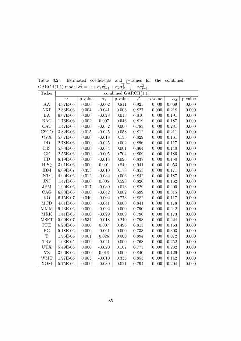
Table 3.2: Estimated coefficients and p-values for the combined
GARCH(1,1) model σ2t = ω + α1r2t−1 + α2σ2P,t−1 + βσ2t−1.
Ticker combined GARCH(1,1)ω p-value α1 p-value β p-value α2 p-value
AA 4.37E-06 0.000 -0.002 0.811 0.925 0.000 0.069 0.000AXP 2.33E-06 0.004 -0.041 0.003 0.827 0.000 0.218 0.000BA 6.07E-06 0.000 -0.028 0.013 0.810 0.000 0.191 0.000
BAC 1.76E-06 0.002 0.007 0.546 0.819 0.000 0.187 0.000CAT 1.47E-05 0.000 -0.052 0.000 0.783 0.000 0.231 0.000
CSCO 3.82E-06 0.015 -0.025 0.058 0.812 0.000 0.211 0.000CVX 5.67E-06 0.000 -0.018 0.135 0.829 0.000 0.161 0.000DD 2.78E-06 0.000 -0.025 0.002 0.896 0.000 0.117 0.000DIS 5.88E-06 0.000 -0.034 0.001 0.864 0.000 0.140 0.000GE 2.56E-06 0.000 -0.005 0.704 0.809 0.000 0.186 0.000HD 8.19E-06 0.000 -0.018 0.095 0.837 0.000 0.150 0.000
HPQ 3.01E-06 0.000 0.001 0.849 0.941 0.000 0.053 0.000IBM 6.69E-07 0.353 -0.010 0.178 0.853 0.000 0.171 0.000
INTC 4.90E-06 0.012 -0.032 0.006 0.842 0.000 0.187 0.000JNJ 1.47E-06 0.000 0.005 0.598 0.826 0.000 0.162 0.000JPM 1.90E-06 0.017 -0.030 0.013 0.829 0.000 0.200 0.000CAG 6.83E-06 0.000 -0.042 0.002 0.699 0.000 0.315 0.000KO 6.15E-07 0.046 -0.002 0.773 0.882 0.000 0.117 0.000
MCD 4.61E-06 0.000 -0.041 0.000 0.841 0.000 0.178 0.000MMM 9.43E-06 0.000 -0.092 0.000 0.790 0.000 0.242 0.000MRK 1.41E-05 0.000 -0.029 0.009 0.796 0.000 0.173 0.000MSFT 5.69E-07 0.534 -0.018 0.240 0.798 0.000 0.224 0.000PFE 6.28E-06 0.000 0.007 0.496 0.813 0.000 0.163 0.000PG 5.18E-06 0.000 -0.061 0.000 0.733 0.000 0.303 0.000T 1.95E-06 0.001 0.026 0.000 0.894 0.000 0.072 0.000
TRV 1.03E-05 0.000 -0.041 0.000 0.768 0.000 0.252 0.000UTX 5.49E-06 0.000 -0.020 0.107 0.773 0.000 0.232 0.000VZ 3.96E-06 0.000 0.018 0.009 0.840 0.000 0.129 0.000
WMT 1.97E-06 0.003 -0.010 0.338 0.855 0.000 0.142 0.000XOM 5.75E-06 0.000 -0.030 0.021 0.794 0.000 0.204 0.000
85
Out-of-sample forecasting performance
As seen in the previous subsection, the modified GARCH(1,1) outperforms
its standard counterpart in the in-sample fit of the data. The next obvious
question is the comparison of the predictive ability of these models. To
answer this question, we compare one-day ahead forecasts of the models
(3.5) and (3.7) with squared returns as a benchmark. Results are presented
in the Table 3.3.
As we can see from Table 3.3, the RGARCH(1,1) model clearly outper-
forms GARCH(1,1). All the cases (stock-estimation window pairs) when the
difference is statistically significant favour the RGARCH model. Note that
the reason why the difference is often insignificant is not because the models
are indistinguishable, but because squared returns (a very noisy volatil-
ity proxy) make the distinction between any two volatility models difficult.
In fact the RGARCH model provides larger improvement to GARCH(1,1)
model than any of the studied GARCH models.
The next obvious question is how our RGARCH performs relative to
other more complicated GARCH models. Even though a detailed answer
to this question is behyond the scope of this paper, we provide some basic
comparison. We now compare the RGARCH model (3.10) not only with
the basic GARCH model (3.5), but with its other versions (3.12)-(3.16) too.
We chose an estimation window equal to 400. A shorter estimation window
would favour the RGARCH model even more. A too long estimation win-
dow is not desirable, because, as Table 3.3 documents, volatility forecasting
becomes less precise when we use a too long estimation window.
As we can see from Table 3.4, the comparison of the RGARCH model
with other GARCH models is very similar to previous comparison. The
RGARCH model typically outperforms other GARCH models. When we
86
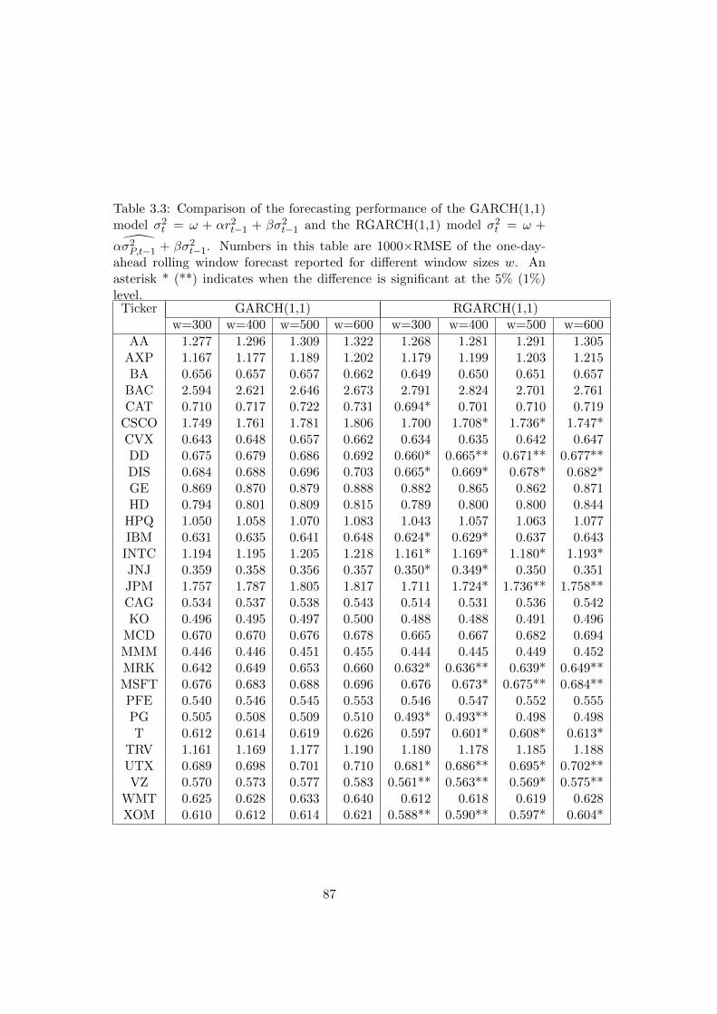
Table 3.3: Comparison of the forecasting performance of the GARCH(1,1)model σ2t = ω + αr2t−1 + βσ2t−1 and the RGARCH(1,1) model σ2t = ω +
ασ2P,t−1 + βσ2t−1. Numbers in this table are 1000×RMSE of the one-day-ahead rolling window forecast reported for different window sizes w. Anasterisk * (**) indicates when the difference is significant at the 5% (1%)level.
Ticker GARCH(1,1) RGARCH(1,1)w=300 w=400 w=500 w=600 w=300 w=400 w=500 w=600
AA 1.277 1.296 1.309 1.322 1.268 1.281 1.291 1.305AXP 1.167 1.177 1.189 1.202 1.179 1.199 1.203 1.215BA 0.656 0.657 0.657 0.662 0.649 0.650 0.651 0.657
BAC 2.594 2.621 2.646 2.673 2.791 2.824 2.701 2.761CAT 0.710 0.717 0.722 0.731 0.694* 0.701 0.710 0.719
CSCO 1.749 1.761 1.781 1.806 1.700 1.708* 1.736* 1.747*CVX 0.643 0.648 0.657 0.662 0.634 0.635 0.642 0.647DD 0.675 0.679 0.686 0.692 0.660* 0.665** 0.671** 0.677**DIS 0.684 0.688 0.696 0.703 0.665* 0.669* 0.678* 0.682*GE 0.869 0.870 0.879 0.888 0.882 0.865 0.862 0.871HD 0.794 0.801 0.809 0.815 0.789 0.800 0.800 0.844
HPQ 1.050 1.058 1.070 1.083 1.043 1.057 1.063 1.077IBM 0.631 0.635 0.641 0.648 0.624* 0.629* 0.637 0.643
INTC 1.194 1.195 1.205 1.218 1.161* 1.169* 1.180* 1.193*JNJ 0.359 0.358 0.356 0.357 0.350* 0.349* 0.350 0.351JPM 1.757 1.787 1.805 1.817 1.711 1.724* 1.736** 1.758**CAG 0.534 0.537 0.538 0.543 0.514 0.531 0.536 0.542KO 0.496 0.495 0.497 0.500 0.488 0.488 0.491 0.496
MCD 0.670 0.670 0.676 0.678 0.665 0.667 0.682 0.694MMM 0.446 0.446 0.451 0.455 0.444 0.445 0.449 0.452MRK 0.642 0.649 0.653 0.660 0.632* 0.636** 0.639* 0.649**MSFT 0.676 0.683 0.688 0.696 0.676 0.673* 0.675** 0.684**PFE 0.540 0.546 0.545 0.553 0.546 0.547 0.552 0.555PG 0.505 0.508 0.509 0.510 0.493* 0.493** 0.498 0.498T 0.612 0.614 0.619 0.626 0.597 0.601* 0.608* 0.613*
TRV 1.161 1.169 1.177 1.190 1.180 1.178 1.185 1.188UTX 0.689 0.698 0.701 0.710 0.681* 0.686** 0.695* 0.702**VZ 0.570 0.573 0.577 0.583 0.561** 0.563** 0.569* 0.575**
WMT 0.625 0.628 0.633 0.640 0.612 0.618 0.619 0.628XOM 0.610 0.612 0.614 0.621 0.588** 0.590** 0.597* 0.604*
87
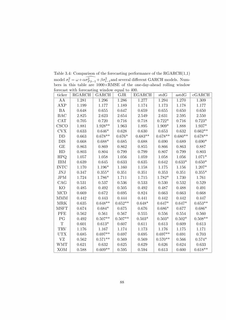
Table 3.4: Comparison of the forecasting performance of the RGARCH(1,1)
model σ2t = ω+ασ2P,t−1+βσ2t−1and several different GARCH models. Num-bers in this table are 1000×RMSE of the one-day-ahead rolling windowforecast with forecasting window equal to 400.
ticker RGARCH GARCH GJR EGARCH stdG astdG cGARCH
AA 1.281 1.296 1.286 1.277 1.294 1.270 1.309AXP 1.199 1.177 1.189 1.174 1.173 1.178 1.177BA 0.648 0.655 0.647 0.659 0.655 0.650 0.650
BAC 2.825 2.623 2.654 2.549 2.631 2.595 2.550CAT 0.705 0.720 0.716 0.718 0.722* 0.716 0.723*
CSCO 1.881 1.928** 1.963 1.895 1.909* 1.888 1.937*CVX 0.633 0.646* 0.628 0.630 0.653 0.632 0.662**DD 0.663 0.678** 0.676* 0.683** 0.678** 0.680** 0.678**DIS 0.668 0.688* 0.685 0.688 0.690 0.689 0.690*GE 0.863 0.869 0.862 0.855 0.866 0.863 0.887HD 0.803 0.804 0.799 0.799 0.807 0.799 0.803
HPQ 1.057 1.058 1.056 1.059 1.058 1.056 1.071*IBM 0.639 0.645 0.633 0.635 0.642 0.633* 0.650*
INTC 1.170 1.196* 1.160 1.158 1.175 1.156 1.207*JNJ 0.347 0.355* 0.351 0.351 0.353 0.351 0.355*JPM 1.724 1.786* 1.711 1.715 1.782* 1.730 1.761CAG 0.531 0.537 0.536 0.533 0.530 0.532 0.529KO 0.485 0.492 0.505 0.492 0.487 0.488 0.491
MCD 0.669 0.672 0.695 0.824 0.663 0.663 0.668MMM 0.442 0.443 0.444 0.441 0.442 0.442 0.447MRK 0.635 0.648** 0.652** 0.648* 0.647* 0.647* 0.653**MSFT 0.674 0.684* 0.675 0.676 0.686* 0.677 0.686*PFE 0.562 0.561 0.567 0.555 0.556 0.554 0.560PG 0.492 0.507** 0.507** 0.503* 0.503* 0.502* 0.508**T 0.601 0.613* 0.607 0.611 0.613 0.609 0.613
TRV 1.176 1.167 1.174 1.173 1.176 1.175 1.171UTX 0.685 0.697** 0.697 0.695 0.697** 0.691 0.703VZ 0.562 0.571** 0.569 0.569 0.570** 0.566 0.574*
WMT 0.621 0.632 0.625 0.629 0.626 0.624 0.633XOM 0.588 0.609** 0.595 0.594 0.613 0.600 0.618**
88

consider only the cases where the difference is statistically significant, the
RGACH model always outperforms all other studied GARCH models. More-
over, the comparison of the RGARCH model with other GARCH models
shows that the RGARCH model typically either performs better than any
of the competing GARCH models or worse than all of them. Therefore
comparison of the RGARCH model with the basic GARCH(1,1) model can
to some extend serve as an evaluation of the overall performance of the
RGARCH model.
The results summarized in Tables 3.3 and 3.4 show the superior perfor-
mance of the RGARCH model. However, the improvement in the RGARCH
model in comparison to the basic GARCH(1,1) model seems to be rather
small at the first glance. Even though the RGARCH model outperforms the
basic GARCH(1,1) model in most cases, the average improvement of the
RMSE reported in Table 3.3 is just approximately 1%. This could give us a
first impression that the improvement of the RGARCH(1,1) model over the
GARCH(1,1) model is rather small.
However, this first impression is misleading. There is a problem with this
standard evaluation procedure, where we compare the forecasted volatilility
with the squared returns. Even though the squared returns are unbiased
estimates of the volatility, they are very noisy. There are two ways to deal
with this problem. The most natural solution to this problem is to use
the true volatility as a benchmark, or, if unavailable, some other less noisy
volatility proxy. This is what we do in the following subsections. However,
due to the data availability constraint, we cannot do this for the 30 stocks
we just studied. Therefore before we proceed to to next subsection dealing
with stock indices (for which the realized variances are available) data, we
suggest an alternative measure for the comparison of the basic GARCH(1,1)
89
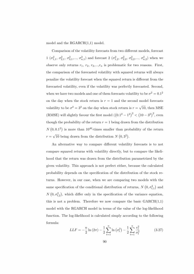
model and the RGARCH(1,1) model.
Comparison of the volatility forecasts from two different models, forecast
1 (σ21,1, σ22,1, σ
23,1,..., σ
2n,1) and forecast 2 (σ21,2, σ
22,2, σ
23,2,..., σ
2n,2) when we
observe only returns r1, r2, r2,...,rn is problematic for two reasons. First,
the comparison of the forecasted volatility with squared returns will always
penalize the volatility forecast when the squared return is different from the
forecasted volatility, even if the volatility was perfectly forecasted. Second,
when we have two models and one of them forecasts volatility to be σ2 = 0.12
on the day when the stock return is r = 1 and the second model forecasts
volatility to be σ2 = 32 on the day when stock return is r =√
10, then MSE
(RMSE) will slightly favour the first model ((0.12 − 12
)2<(10− 32
)2, even
though the probability of the return r = 1 being drawn from the distribution
N(0, 0.12
)is more than 1040-times smaller than probability of the return
r =√
10 being drawn from the distribution N(0, 32
).
An alternative way to compare different volatility forecasts is to not
compare squared returns with volatility directly, but to compare the likeli-
hood that the return was drawn from the distribution parametrized by the
given volatility. This approach is not perfect either, because the calculated
probability depends on the specification of the distribution of the stock re-
turns. However, in our case, when we are comparing two models with the
same specification of the conditional distribution of returns, N(0, σ2t,1
)and
N(0, σ2t,2
), which differ only in the specification of the variance equation,
this is not a problem. Therefore we now compare the basic GARCH(1,1)
model with the RGARCH model in terms of the value of the log-likelihood
function. The log-likelihood is calculated simply according to the following
formula:
LLF = −n2
ln (2π)− 1
2
n∑t=1
ln(σ2t)− 1
2
n∑t=1
r2tσ2t
(3.27)
90
where σ2t is the volatility forecasted from the studied volatility model (using
past information only).
Table 3.5 confirms our previous comparison between the RGARCH model
and the standard GARCH model. The RGARCH model outperforms the
standard GARCH(1,1) model for basically every single stock and for every
estimation window (in 119 of 120 stock-estimation window couples).
3.3.2 Stock indices
In addition to the individual stocks of the Dow Jones Industrial Average
stock index we decided to compare the performance of the RGARCH model
to the standard GARCH model on the major world indices (French CAC
40, German DAX, Japanese Nikkei 225, Britain’s FTSE 100 and American
DJI and NASDAQ 100). There are two reasons for this. First, volatility
dynamics is generally different for individual stocks and for the whole stock
markets. Second, estimates of realized variance, which is a proxy for the
true variance, are publicly available for these indices12. Open, high, low
and close prices are downloaded from finance.yahoo.com. Data covers the
period January 3, 1993 - April 27, 2009 for open, high and low prices and
the period January 3, 1996 - April 27, 2009 for the realized variance. Due
to small differences in trading days in different markets, the number of
observations varies accordingly.
For the in-sample analysis we use the data ranging from January 3, 1993
to April 27, 2009. Volatility forecast is always performed for the volatilities
forecasted for the period January 3, 1996 - April 27, 2009. However, esti-
mates of realized variance are not available for some trading days. These
days are included in the volatility forecast comparison when squared returns
12Heber, Gerd, Asger Lunde, Neil Shephard and Kevin K. Sheppard (2009) ”Oxford-Man Institute’s Realized Library”, Oxford-Man Institute, University of Oxford
91
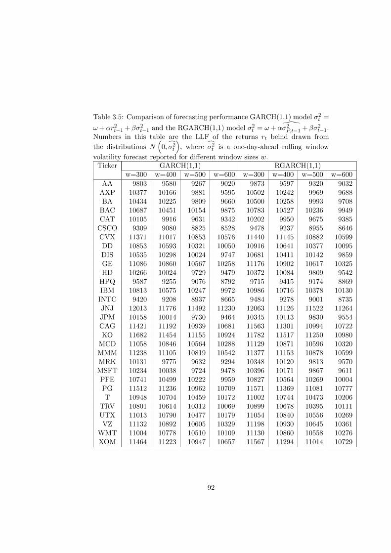
Table 3.5: Comparison of forecasting performance GARCH(1,1) model σ2t =
ω+αr2t−1 + βσ2t−1 and the RGARCH(1,1) model σ2t = ω+ασ2P,t−1 + βσ2t−1.Numbers in this table are the LLF of the returns rt beind drawn from
the distributions N(
0, σ2t
), where σ2t is a one-day-ahead rolling window
volatility forecast reported for different window sizes w.Ticker GARCH(1,1) RGARCH(1,1)
w=300 w=400 w=500 w=600 w=300 w=400 w=500 w=600
AA 9803 9580 9267 9020 9873 9597 9320 9032AXP 10377 10166 9881 9595 10502 10242 9969 9688BA 10434 10225 9809 9660 10500 10258 9993 9708
BAC 10687 10451 10154 9875 10783 10527 10236 9949CAT 10105 9916 9631 9342 10202 9950 9675 9385
CSCO 9309 9080 8825 8528 9478 9237 8955 8646CVX 11371 11017 10853 10576 11440 11145 10882 10599DD 10853 10593 10321 10050 10916 10641 10377 10095DIS 10535 10298 10024 9747 10681 10411 10142 9859GE 11086 10860 10567 10258 11176 10902 10617 10325HD 10266 10024 9729 9479 10372 10084 9809 9542
HPQ 9587 9255 9076 8792 9715 9415 9174 8869IBM 10813 10575 10247 9972 10986 10716 10378 10130
INTC 9420 9208 8937 8665 9484 9278 9001 8735JNJ 12013 11776 11492 11230 12063 11126 11522 11264JPM 10158 10014 9730 9464 10345 10113 9830 9554CAG 11421 11192 10939 10681 11563 11301 10994 10722KO 11682 11454 11155 10924 11782 11517 11250 10980
MCD 11058 10846 10564 10288 11129 10871 10596 10320MMM 11238 11105 10819 10542 11377 11153 10878 10599MRK 10131 9775 9632 9294 10348 10120 9813 9570MSFT 10234 10038 9724 9478 10396 10171 9867 9611PFE 10741 10499 10222 9959 10827 10564 10269 10004PG 11512 11236 10962 10709 11571 11369 11081 10777T 10948 10704 10459 10172 11002 10744 10473 10206
TRV 10801 10614 10312 10069 10899 10678 10395 10111UTX 11013 10790 10477 10179 11054 10840 10556 10269VZ 11132 10892 10605 10329 11198 10930 10645 10361
WMT 11004 10778 10510 10109 11130 10860 10558 10276XOM 11464 11223 10947 10657 11567 11294 11014 10729
92
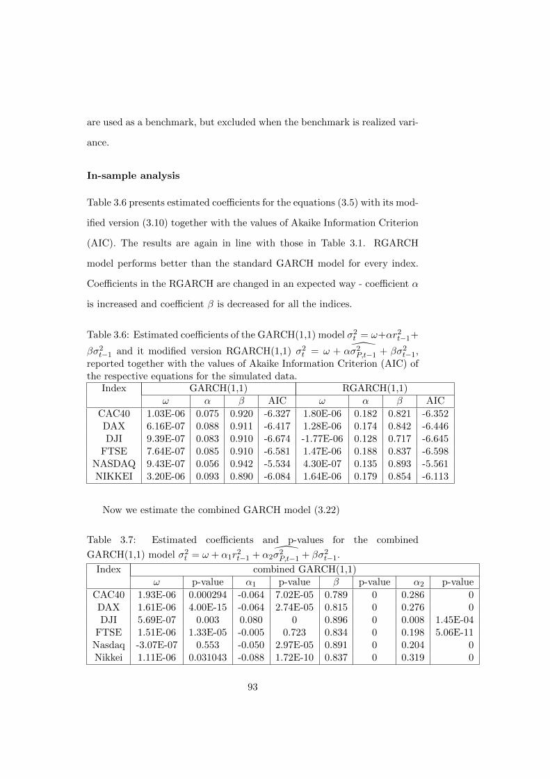
are used as a benchmark, but excluded when the benchmark is realized vari-
ance.
In-sample analysis
Table 3.6 presents estimated coefficients for the equations (3.5) with its mod-
ified version (3.10) together with the values of Akaike Information Criterion
(AIC). The results are again in line with those in Table 3.1. RGARCH
model performs better than the standard GARCH model for every index.
Coefficients in the RGARCH are changed in an expected way - coefficient α
is increased and coefficient β is decreased for all the indices.
Table 3.6: Estimated coefficients of the GARCH(1,1) model σ2t = ω+αr2t−1+
βσ2t−1 and it modified version RGARCH(1,1) σ2t = ω + ασ2P,t−1 + βσ2t−1,reported together with the values of Akaike Information Criterion (AIC) ofthe respective equations for the simulated data.
Index GARCH(1,1) RGARCH(1,1)ω α β AIC ω α β AIC
CAC40 1.03E-06 0.075 0.920 -6.327 1.80E-06 0.182 0.821 -6.352DAX 6.16E-07 0.088 0.911 -6.417 1.28E-06 0.174 0.842 -6.446DJI 9.39E-07 0.083 0.910 -6.674 -1.77E-06 0.128 0.717 -6.645
FTSE 7.64E-07 0.085 0.910 -6.581 1.47E-06 0.188 0.837 -6.598NASDAQ 9.43E-07 0.056 0.942 -5.534 4.30E-07 0.135 0.893 -5.561NIKKEI 3.20E-06 0.093 0.890 -6.084 1.64E-06 0.179 0.854 -6.113
Now we estimate the combined GARCH model (3.22)
Table 3.7: Estimated coefficients and p-values for the combined
GARCH(1,1) model σ2t = ω + α1r2t−1 + α2σ2P,t−1 + βσ2t−1.
Index combined GARCH(1,1)ω p-value α1 p-value β p-value α2 p-value
CAC40 1.93E-06 0.000294 -0.064 7.02E-05 0.789 0 0.286 0DAX 1.61E-06 4.00E-15 -0.064 2.74E-05 0.815 0 0.276 0DJI 5.69E-07 0.003 0.080 0 0.896 0 0.008 1.45E-04
FTSE 1.51E-06 1.33E-05 -0.005 0.723 0.834 0 0.198 5.06E-11Nasdaq -3.07E-07 0.553 -0.050 2.97E-05 0.891 0 0.204 0Nikkei 1.11E-06 0.031043 -0.088 1.72E-10 0.837 0 0.319 0
93
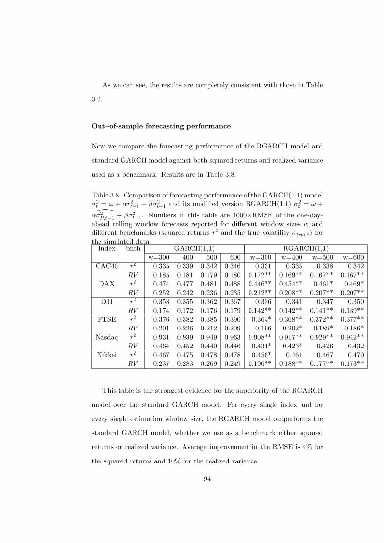
As we can see, the results are completely consistent with those in Table
3.2.
Out–of-sample forecasting performance
Now we compare the forecasting performance of the RGARCH model and
standard GARCH model against both squared returns and realized variance
used as a benchmark. Results are in Table 3.8.
Table 3.8: Comparison of forecasting performance of the GARCH(1,1) modelσ2t = ω + αr2t−1 + βσ2t−1 and its modified version RGARCH(1,1) σ2t = ω +
ασ2P,t−1 + βσ2t−1. Numbers in this table are 1000×RMSE of the one-day-ahead rolling window forecasts reported for different window sizes w anddifferent benchmarks (squared returns r2 and the true volatility σtrue2) forthe simulated data.
Index bnch GARCH(1,1) RGARCH(1,1)w=300 400 500 600 w=300 w=400 w=500 w=600
CAC40 r2 0.335 0.339 0.342 0.346 0.331 0.335 0.338 0.342RV 0.185 0.181 0.179 0.180 0.172** 0.169** 0.167** 0.167**
DAX r2 0.474 0.477 0.481 0.488 0.446** 0.454** 0.461* 0.469*RV 0.252 0.242 0.236 0.235 0.212** 0.208** 0.207** 0.207**
DJI r2 0.353 0.355 0.362 0.367 0.336 0.341 0.347 0.350RV 0.174 0.172 0.176 0.179 0.142** 0.142** 0.141** 0.139**
FTSE r2 0.376 0.382 0.385 0.390 0.364* 0.368** 0.372** 0.377**RV 0.201 0.226 0.212 0.209 0.196 0.202* 0.189* 0.186*
Nasdaq r2 0.931 0.939 0.949 0.963 0.908** 0.917** 0.929** 0.942**RV 0.464 0.452 0.440 0.446 0.431* 0.423* 0.426 0.432
Nikkei r2 0.467 0.475 0.478 0.478 0.456* 0.461 0.467 0.470RV 0.237 0.283 0.269 0.249 0.196** 0.188** 0.177** 0.173**
This table is the strongest evidence for the superiority of the RGARCH
model over the standard GARCH model. For every single index and for
every single estimation window size, the RGARCH model outperforms the
standard GARCH model, whether we use as a benchmark either squared
returns or realized variance. Average improvement in the RMSE is 4% for
the squared returns and 10% for the realized variance.
94
3.3.3 Simulated data
In reality, we can never know for sure what the true volatility was, but when
we simulate the data, then we know the true volatility exactly. Simulation
therefore provides a convinient tool to study different volatility models. On
the other hand, the issue with simulation is always how close are simulated
data to the real world. In order to convince the reader that the simulated
data we chose are close to reality, we do not decide on the simulation by
ourselves. We borrow the credibility of Alizadeh, Brand and Diebold (2002)
and simulate the data in the following way. First we simulate the volatility
process
lnσt = lnσ + ρH (lnσt−1 − lnσ) + µεt−1 (3.28)
with parameters ln (σ) = −2.5, ρH = 0.985 and µ = 0.75/√
257 = 0.048. Af-
terwards we simulate for every day t = 1, 2, ..., 100000 a Brownian motion13
with zero drift term and diffusion term equal to σt. We save the highest, the
lowest and the final value of this Brownian motion. Both equation (3.28) and
the parameter values are taken from Alizadeh, Brand and Diebold (2002),
who found that the volatility dynamics (3.28) is broadly consitent with lit-
erature on stochastic volatility. Note that there are no opening jumps in
this these simulated data.
Note that the volatility process (3.28) does not favour directly either
of the competing models (3.5) and (3.10). Volatility gradually evolves over
the time, and neither past returns nor past high or low prices influence the
future volatility in any way.
13We use 100000 discrete steps for the approximation of the continuous Brownian mo-tion.
95
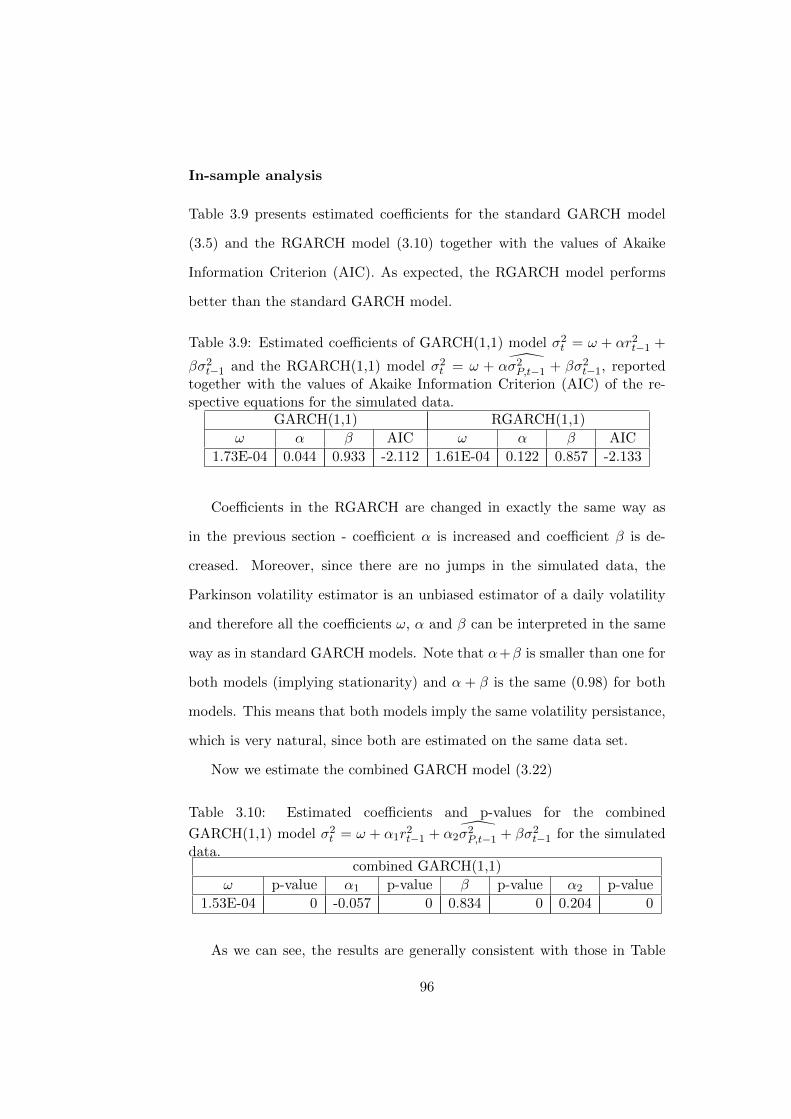
In-sample analysis
Table 3.9 presents estimated coefficients for the standard GARCH model
(3.5) and the RGARCH model (3.10) together with the values of Akaike
Information Criterion (AIC). As expected, the RGARCH model performs
better than the standard GARCH model.
Table 3.9: Estimated coefficients of GARCH(1,1) model σ2t = ω + αr2t−1 +
βσ2t−1 and the RGARCH(1,1) model σ2t = ω + ασ2P,t−1 + βσ2t−1, reportedtogether with the values of Akaike Information Criterion (AIC) of the re-spective equations for the simulated data.
GARCH(1,1) RGARCH(1,1)
ω α β AIC ω α β AIC
1.73E-04 0.044 0.933 -2.112 1.61E-04 0.122 0.857 -2.133
Coefficients in the RGARCH are changed in exactly the same way as
in the previous section - coefficient α is increased and coefficient β is de-
creased. Moreover, since there are no jumps in the simulated data, the
Parkinson volatility estimator is an unbiased estimator of a daily volatility
and therefore all the coefficients ω, α and β can be interpreted in the same
way as in standard GARCH models. Note that α+β is smaller than one for
both models (implying stationarity) and α + β is the same (0.98) for both
models. This means that both models imply the same volatility persistance,
which is very natural, since both are estimated on the same data set.
Now we estimate the combined GARCH model (3.22)
Table 3.10: Estimated coefficients and p-values for the combined
GARCH(1,1) model σ2t = ω + α1r2t−1 + α2σ2P,t−1 + βσ2t−1 for the simulated
data.combined GARCH(1,1)
ω p-value α1 p-value β p-value α2 p-value
1.53E-04 0 -0.057 0 0.834 0 0.204 0
As we can see, the results are generally consistent with those in Table
96
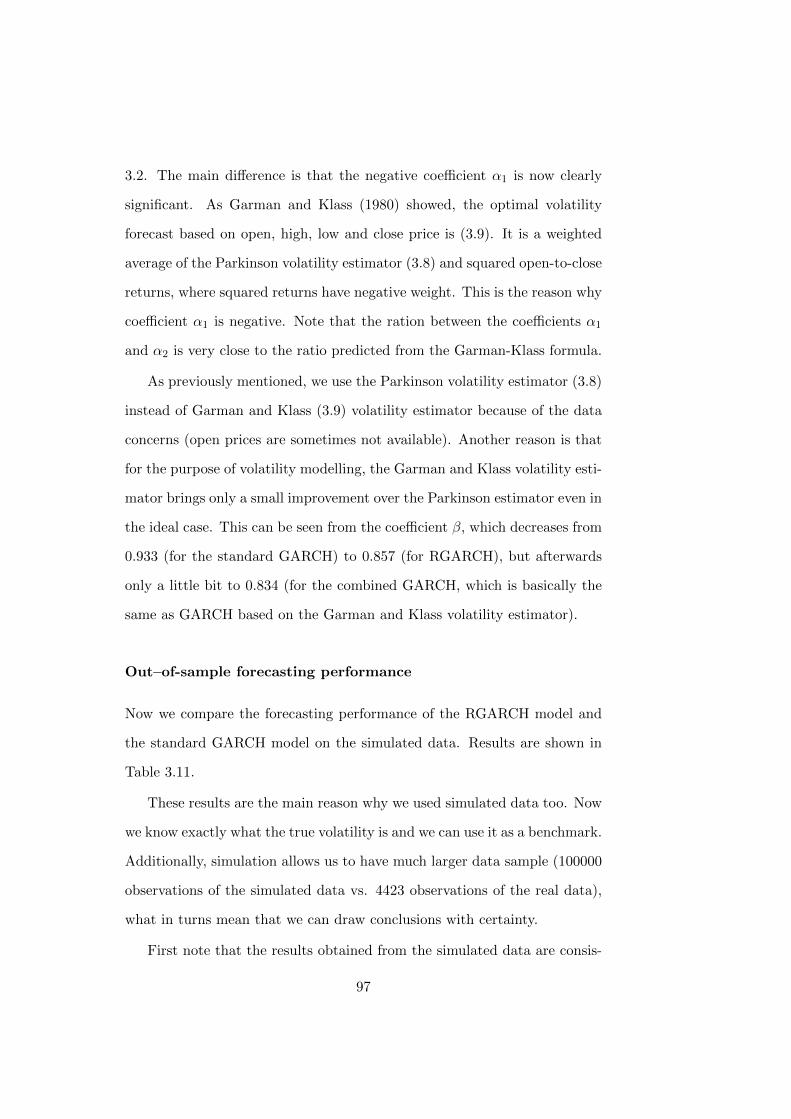
3.2. The main difference is that the negative coefficient α1 is now clearly
significant. As Garman and Klass (1980) showed, the optimal volatility
forecast based on open, high, low and close price is (3.9). It is a weighted
average of the Parkinson volatility estimator (3.8) and squared open-to-close
returns, where squared returns have negative weight. This is the reason why
coefficient α1 is negative. Note that the ration between the coefficients α1
and α2 is very close to the ratio predicted from the Garman-Klass formula.
As previously mentioned, we use the Parkinson volatility estimator (3.8)
instead of Garman and Klass (3.9) volatility estimator because of the data
concerns (open prices are sometimes not available). Another reason is that
for the purpose of volatility modelling, the Garman and Klass volatility esti-
mator brings only a small improvement over the Parkinson estimator even in
the ideal case. This can be seen from the coefficient β, which decreases from
0.933 (for the standard GARCH) to 0.857 (for RGARCH), but afterwards
only a little bit to 0.834 (for the combined GARCH, which is basically the
same as GARCH based on the Garman and Klass volatility estimator).
Out–of-sample forecasting performance
Now we compare the forecasting performance of the RGARCH model and
the standard GARCH model on the simulated data. Results are shown in
Table 3.11.
These results are the main reason why we used simulated data too. Now
we know exactly what the true volatility is and we can use it as a benchmark.
Additionally, simulation allows us to have much larger data sample (100000
observations of the simulated data vs. 4423 observations of the real data),
what in turns mean that we can draw conclusions with certainty.
First note that the results obtained from the simulated data are consis-
97
Table 3.11: Comparison of the forecasting performance of the GARCH(1,1)model σ2t = ω + αr2t−1 + βσ2t−1 and it modified version RGARCH(1,1) σ2t =
ω+ασ2P,t−1 +βσ2t−1. Numbers in this table are 1000×RMSE of the one-day-ahead rolling window forecasts reported for different window sizes w anddifferent benchmarks squared returns (r2) and the true volatility (σ2true) forthe simulated data. The differences in MSE are significant at any significancelevel.bnch GARCH(1,1) RGARCH(1,1) σ2true
w=300 400 500 600 300 400 500 600
r2 11.76 11.72 11.69 11.66 11.64 11.60 11.56 11.54 11.34σ2true 2.95 2.88 2.80 2.72 2.47 2.30 2.20 2.12 0
tent with results in Table 3.3. Table 3.3 shows that the RGARCH model
outperforms the standard GARCH model most of the time. Since the sim-
ulated data are much larger, we basically got rid of the noise and now we
can see exactly how much better the RGARCH performs. The improvement
seems to be small, just around 1% decrease in RMSE, when we use squared
returns as a benchmark. However, use of the true volatility as a benchmark
shows that the real improvement of the RGARCH in comparison to the
standard GARCH model is much larger, around 20%.
In fact, the mean squared error (MSE) between the forecasted volatility
(σ2) and squared returns (r2) can be rewritten in the following way:
MSE(σ2, r2
)= MSE
(σ2, σ2true
)+MSE
(σ2true, r
2)
(3.29)
where r2 is squared return and σ2true is the true volatility. When squared
returns are used as a benchmark, then the second term typically dominates
and it is therefore difficult to choose between competing volatility models
based on the MSE (RMSE).
98
3.4 Summary
The goal of this paper was to show a simple, effective and general way to
incorporate range (the difference between highest and the lowest price of the
day) into the standard GARCH volatility models. We illustrated our idea on
the GARCH(1,1) model, which we modify and create a Range GARCH(1,1)
model. Empirical tests performed on 30 stocks, 6 stock indices and simu-
lated data show that the RGARCH model strongly outperforms the standard
GARCH model, both in the in-sample fit and in the out-of-sample forecast-
ing. The main intuition behind this result is that replacing squared returns
by less noisy volatility proxy has two advantages. First, putting more pri-
cise volatility proxy into a given model obviously helps. Second, when the
model is estimated, more weight than before will be attributed to the most
recent volatility estimate, because this estimate is now less noisy. As a conse-
quence, this model can adjust more quickly to the changes of volatility. This
is particularly relevant, because volatility forecasting is most important in
situations when volatility changes the most. RGARCH model outperforms
the standard GARCH model (and basically any of the studied GARCH
models). The main advantage of our model is that it provides both high
precision of range as a volatility proxy with simplicity and ease of estima-
tion of the standard GARCH model. This model offers significantly increase
precision in volatility modelling at almost no costs: additional required data
(high and low prices) are typically widely available and the model itself can
be easily estimated using standard econometric sofware, e.g. Eviews, R or
OxMetrics. Therefore we encourage both academics and practitioners to use
the RGARCH model instead of the standard GARCH model whenever high
and low data are available.
99

3.5 Appendix
All the estimations in previous parts of the paper were based on the open-to-
close returns, which means that all the previous results are about volatility
of the trading part of the day. However, this appendix (Table 3.12 - Table
3.19) documents that all the conclusions remain basically the same when our
interest is daily (close-to-close) volatility. All the results confirm superiority
of the RGARCH model. The RGARCH model is compared with standard
GARCH models (mostly GARCH(1,1) model) when both are estimated on
daily data and benchmark is squared daily (close-to-close) returns.
100
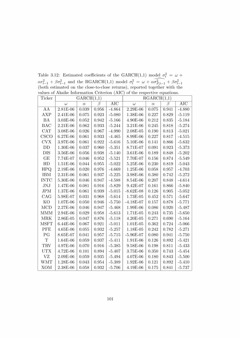
Table 3.12: Estimated coefficients of the GARCH(1,1) model σ2t = ω +
αr2t−1 + βσ2t−1 and the RGARCH(1,1) model σ2t = ω + ασ2P,t−1 + βσ2t−1(both estimated on the close-to-close returns), reported together with thevalues of Akaike Information Criterion (AIC) of the respective equations.
Ticker GARCH(1,1) RGARCH(1,1)ω α β AIC ω α β AIC
AA 2.81E-06 0.039 0.956 -4.864 2.29E-06 0.075 0.941 -4.880AXP 2.41E-06 0.075 0.923 -5.080 1.38E-06 0.227 0.829 -5.119BA 3.03E-06 0.052 0.942 -5.166 4.90E-06 0.212 0.835 -5.184
BAC 2.21E-06 0.062 0.933 -5.244 3.21E-06 0.245 0.818 -5.274CAT 3.08E-06 0.026 0.967 -4.990 2.08E-05 0.190 0.813 -5.021
CSCO 6.27E-06 0.061 0.933 -4.465 8.99E-06 0.227 0.817 -4.515CVX 3.97E-06 0.061 0.922 -5.616 5.10E-06 0.141 0.866 -5.632DD 1.30E-06 0.037 0.960 -5.351 8.71E-07 0.091 0.923 -5.373DIS 3.56E-06 0.056 0.938 -5.140 3.61E-06 0.189 0.848 -5.202GE 7.74E-07 0.046 0.952 -5.521 7.70E-07 0.156 0.874 -5.549HD 1.51E-06 0.044 0.955 -5.022 5.25E-06 0.230 0.819 -5.043
HPQ 2.19E-06 0.020 0.976 -4.669 1.25E-06 0.058 0.957 -4.703IBM 2.31E-06 0.061 0.937 -5.225 3.98E-06 0.380 0.742 -5.272
INTC 5.30E-06 0.046 0.947 -4.588 8.54E-06 0.207 0.848 -4.614JNJ 1.47E-06 0.081 0.916 -5.829 9.42E-07 0.161 0.866 -5.840JPM 1.37E-06 0.061 0.939 -5.015 -8.62E-08 0.126 0.905 -5.052CAG 5.98E-07 0.031 0.968 -5.614 1.73E-05 0.452 0.571 -5.647KO 1.07E-06 0.050 0.946 -5.750 -4.18E-07 0.157 0.878 -5.771
MCD 2.27E-06 0.046 0.947 -5.468 1.99E-06 0.086 0.920 -5.487MMM 2.94E-06 0.029 0.958 -5.613 1.71E-05 0.243 0.735 -5.650MRK 2.86E-05 0.047 0.876 -5.118 4.20E-05 0.271 0.690 -5.164MSFT 6.44E-06 0.067 0.921 -5.011 1.01E-05 0.362 0.724 -5.066PFE 4.65E-06 0.055 0.932 -5.257 1.18E-05 0.242 0.782 -5.271PG 8.65E-07 0.041 0.957 -5.715 -5.96E-07 0.080 0.941 -5.750T 1.64E-06 0.059 0.937 -5.411 1.91E-06 0.126 0.892 -5.421
TRV 4.97E-06 0.070 0.916 -5.385 9.58E-06 0.198 0.811 -5.433UTX 4.72E-06 0.101 0.894 -5.407 3.75E-06 0.350 0.743 -5.454VZ 2.09E-06 0.059 0.935 -5.494 4.07E-06 0.180 0.843 -5.500
WMT 1.28E-06 0.043 0.954 -5.389 1.92E-06 0.121 0.892 -5.410XOM 2.38E-06 0.058 0.932 -5.706 4.19E-06 0.175 0.841 -5.737
101
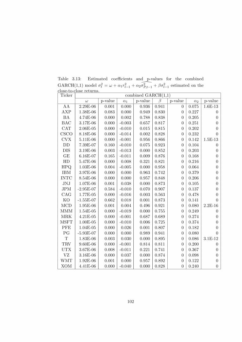
Table 3.13: Estimated coefficients and p-values for the combined
GARCH(1,1) model σ2t = ω + α1r2t−1 + α2σ2P,t−1 + βσ2t−1 estimated on the
close-to-close returns.Ticker combined GARCH(1,1)
ω p-value α1 p-value β p-value α2 p-value
AA 2.29E-06 0.001 0.000 0.936 0.941 0 0.075 1.6E-13AXP 1.38E-06 0.083 0.000 0.949 0.830 0 0.227 0BA 4.74E-06 0.000 0.002 0.788 0.838 0 0.205 0
BAC 3.17E-06 0.000 -0.003 0.657 0.817 0 0.251 0CAT 2.06E-05 0.000 -0.010 0.015 0.815 0 0.202 0
CSCO 8.18E-06 0.000 -0.014 0.002 0.828 0 0.232 0CVX 5.11E-06 0.000 -0.001 0.956 0.866 0 0.142 1.5E-13DD 7.39E-07 0.160 -0.010 0.075 0.923 0 0.104 0DIS 3.19E-06 0.003 -0.013 0.000 0.852 0 0.203 0GE 6.16E-07 0.165 -0.011 0.009 0.876 0 0.168 0HD 5.47E-06 0.000 0.008 0.321 0.821 0 0.216 0
HPQ 1.03E-06 0.004 -0.005 0.000 0.958 0 0.064 0IBM 3.97E-06 0.000 0.000 0.963 0.742 0 0.379 0
INTC 8.54E-06 0.000 0.000 0.957 0.848 0 0.206 0JNJ 1.07E-06 0.001 0.038 0.000 0.873 0 0.105 0JPM -2.95E-07 0.584 -0.010 0.070 0.907 0 0.137 0CAG 1.77E-05 0.000 -0.016 0.003 0.563 0 0.478 0KO -1.55E-07 0.662 0.018 0.001 0.873 0 0.141 0
MCD 1.95E-06 0.001 0.004 0.496 0.921 0 0.080 2.2E-16MMM 1.54E-05 0.000 -0.019 0.000 0.755 0 0.249 0MRK 4.21E-05 0.000 -0.001 0.687 0.689 0 0.274 0MSFT 1.00E-05 0.000 -0.010 0.006 0.725 0 0.374 0PFE 1.04E-05 0.000 0.026 0.001 0.807 0 0.182 0PG -5.93E-07 0.000 0.000 0.989 0.941 0 0.080 0T 1.83E-06 0.003 0.030 0.000 0.895 0 0.086 3.1E-12
TRV 9.60E-06 0.000 -0.001 0.814 0.811 0 0.200 0UTX 3.67E-06 0.008 -0.011 0.221 0.741 0 0.367 0VZ 3.16E-06 0.000 0.037 0.000 0.874 0 0.098 0
WMT 1.92E-06 0.001 0.000 0.957 0.892 0 0.122 0XOM 4.41E-06 0.000 -0.040 0.000 0.828 0 0.240 0
102
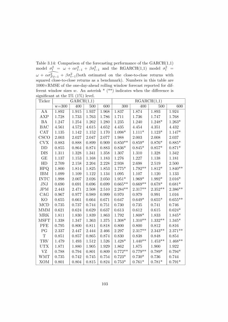
Table 3.14: Comparison of the forecasting performance of the GARCH(1,1)model σ2t = ω + αr2t−1 + βσ2t−1 and the RGARCH(1,1) model σ2t =
ω + ασ2P,t−1 + βσ2t−1(both estimated on the close-to-close returns withsquared close-to-close returns as a benchmark). Numbers in this table are1000×RMSE of the one-day-ahead rolling window forecast reported for dif-ferent window sizes w. An asterisk * (**) indicates when the difference issignificant at the 5% (1%) level.
Ticker GARCH(1,1) RGARCH(1,1)w=300 400 500 600 300 400 500 600
AA 1.892 1.915 1.937 1.968 1.837 1.874 1.893 1.924AXP 1.728 1.733 1.763 1.786 1.711 1.736 1.747 1.768BA 1.247 1.254 1.262 1.280 1.235 1.240 1.248* 1.263*
BAC 4.561 4.572 4.615 4.652 4.435 4.454 4.351 4.432CAT 1.135 1.142 1.152 1.170 1.098* 1.111* 1.123* 1.147*
CSCO 2.003 2.027 2.047 2.077 1.988 2.003 2.008 2.037CVX 0.883 0.888 0.899 0.909 0.850** 0.859* 0.876* 0.885*DD 0.855 0.864 0.874 0.883 0.836* 0.845* 0.857* 0.871*DIS 1.311 1.328 1.341 1.358 1.307 1.310 1.328 1.342GE 1.137 1.153 1.168 1.183 1.276 1.227 1.138 1.181HD 2.709 2.158 2.204 2.228 2.938 2.698 2.519 2.500
HPQ 1.800 1.814 1.825 1.853 1.775* 1.792** 1.812* 1.840**IBM 1.099 1.109 1.122 1.134 1.095 1.107 1.120 1.133
INTC 1.998 2.007 2.026 2.050 1.951* 1.969* 1.992* 2.016*JNJ 0.690 0.691 0.696 0.699 0.665** 0.669** 0.678* 0.681*JPM 2.443 2.471 2.508 2.510 2.284** 2.317** 2.352** 2.386**CAG 0.967 0.977 0.989 0.999 0.970 0.979 0.991 1.016KO 0.655 0.661 0.664 0.671 0.647 0.649* 0.655* 0.655**
MCD 0.735 0.737 0.744 0.751 0.730 0.735 0.741 0.746MMM 0.621 0.624 0.629 0.637 0.613 0.612 0.615 0.624*MRK 1.811 1.830 1.839 1.863 1.792 1.808* 1.833 1.845*MSFT 1.338 1.347 1.363 1.375 1.308* 1.310** 1.332** 1.345*PFE 0.795 0.800 0.811 0.818 0.800 0.800 0.812 0.816PG 2.337 2.447 2.444 2.466 2.297 2.317** 2.343** 2.371**T 0.851 0.857 0.865 0.874 0.830 0.838 0.848 0.854
TRV 1.479 1.493 1.512 1.526 1.428* 1.440** 1.453** 1.468**UTX 1.871 1.880 1.905 1.929 1.862 1.875 1.900 1.922VZ 0.788 0.794 0.801 0.809 0.772** 0.779** 0.789* 0.794*
WMT 0.735 0.742 0.745 0.754 0.723* 0.730* 0.736 0.744XOM 0.801 0.804 0.815 0.824 0.753* 0.761* 0.781* 0.791*
103
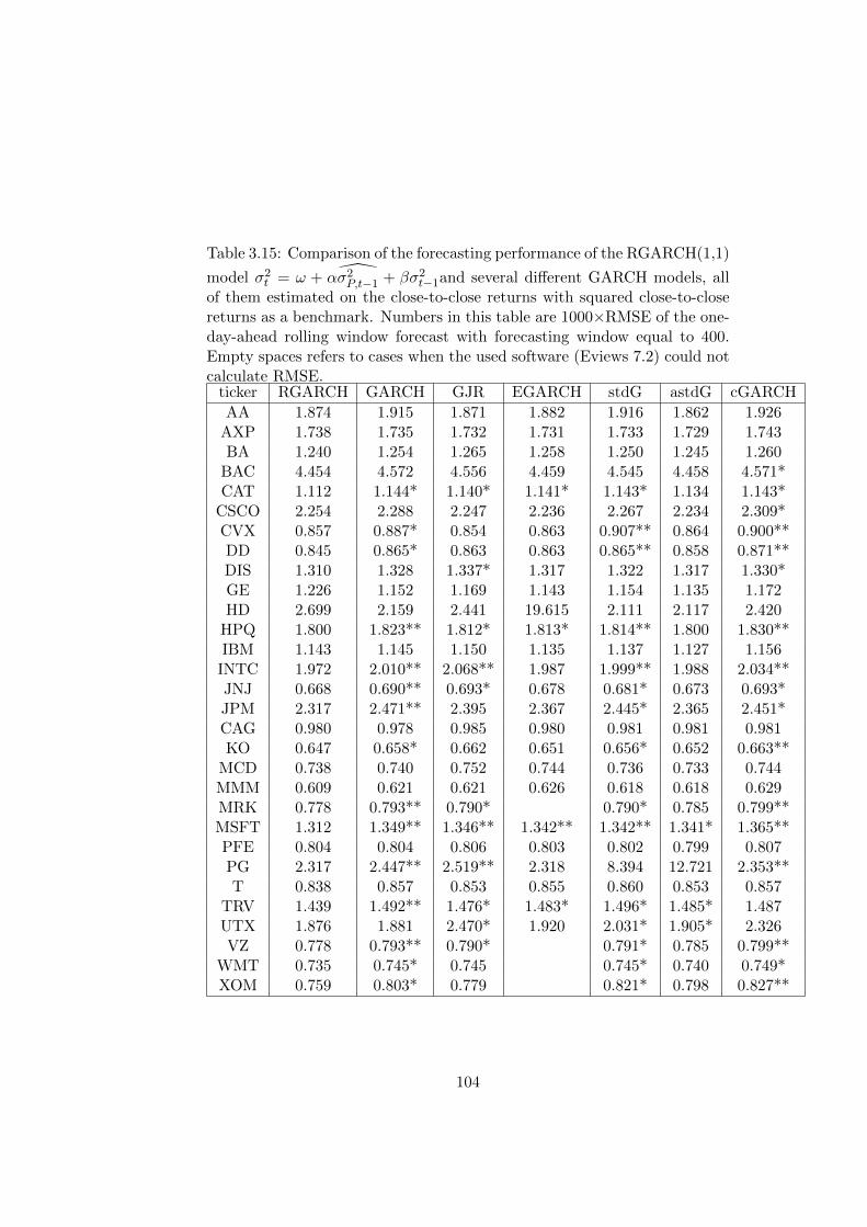
Table 3.15: Comparison of the forecasting performance of the RGARCH(1,1)
model σ2t = ω + ασ2P,t−1 + βσ2t−1and several different GARCH models, allof them estimated on the close-to-close returns with squared close-to-closereturns as a benchmark. Numbers in this table are 1000×RMSE of the one-day-ahead rolling window forecast with forecasting window equal to 400.Empty spaces refers to cases when the used software (Eviews 7.2) could notcalculate RMSE.
ticker RGARCH GARCH GJR EGARCH stdG astdG cGARCH
AA 1.874 1.915 1.871 1.882 1.916 1.862 1.926AXP 1.738 1.735 1.732 1.731 1.733 1.729 1.743BA 1.240 1.254 1.265 1.258 1.250 1.245 1.260
BAC 4.454 4.572 4.556 4.459 4.545 4.458 4.571*CAT 1.112 1.144* 1.140* 1.141* 1.143* 1.134 1.143*
CSCO 2.254 2.288 2.247 2.236 2.267 2.234 2.309*CVX 0.857 0.887* 0.854 0.863 0.907** 0.864 0.900**DD 0.845 0.865* 0.863 0.863 0.865** 0.858 0.871**DIS 1.310 1.328 1.337* 1.317 1.322 1.317 1.330*GE 1.226 1.152 1.169 1.143 1.154 1.135 1.172HD 2.699 2.159 2.441 19.615 2.111 2.117 2.420
HPQ 1.800 1.823** 1.812* 1.813* 1.814** 1.800 1.830**IBM 1.143 1.145 1.150 1.135 1.137 1.127 1.156
INTC 1.972 2.010** 2.068** 1.987 1.999** 1.988 2.034**JNJ 0.668 0.690** 0.693* 0.678 0.681* 0.673 0.693*JPM 2.317 2.471** 2.395 2.367 2.445* 2.365 2.451*CAG 0.980 0.978 0.985 0.980 0.981 0.981 0.981KO 0.647 0.658* 0.662 0.651 0.656* 0.652 0.663**
MCD 0.738 0.740 0.752 0.744 0.736 0.733 0.744MMM 0.609 0.621 0.621 0.626 0.618 0.618 0.629MRK 0.778 0.793** 0.790* 0.790* 0.785 0.799**MSFT 1.312 1.349** 1.346** 1.342** 1.342** 1.341* 1.365**PFE 0.804 0.804 0.806 0.803 0.802 0.799 0.807PG 2.317 2.447** 2.519** 2.318 8.394 12.721 2.353**T 0.838 0.857 0.853 0.855 0.860 0.853 0.857
TRV 1.439 1.492** 1.476* 1.483* 1.496* 1.485* 1.487UTX 1.876 1.881 2.470* 1.920 2.031* 1.905* 2.326VZ 0.778 0.793** 0.790* 0.791* 0.785 0.799**
WMT 0.735 0.745* 0.745 0.745* 0.740 0.749*XOM 0.759 0.803* 0.779 0.821* 0.798 0.827**
104
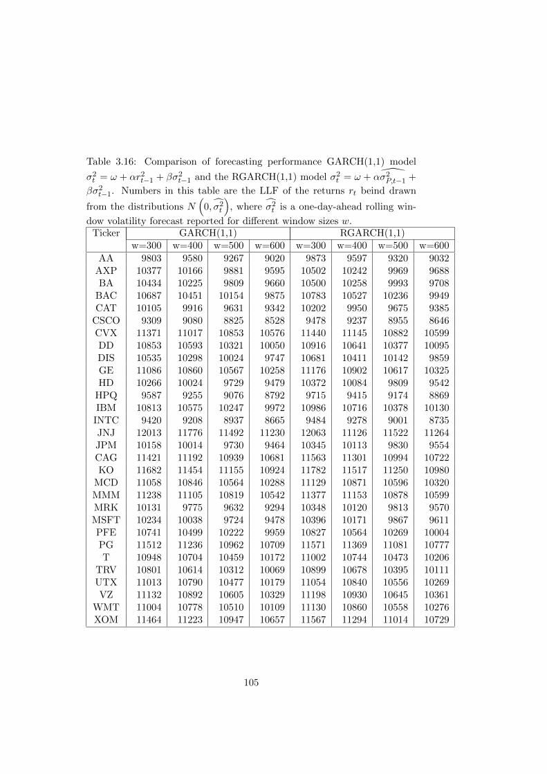
Table 3.16: Comparison of forecasting performance GARCH(1,1) model
σ2t = ω + αr2t−1 + βσ2t−1 and the RGARCH(1,1) model σ2t = ω + ασ2P,t−1 +
βσ2t−1. Numbers in this table are the LLF of the returns rt beind drawn
from the distributions N(
0, σ2t
), where σ2t is a one-day-ahead rolling win-
dow volatility forecast reported for different window sizes w.Ticker GARCH(1,1) RGARCH(1,1)
w=300 w=400 w=500 w=600 w=300 w=400 w=500 w=600
AA 9803 9580 9267 9020 9873 9597 9320 9032AXP 10377 10166 9881 9595 10502 10242 9969 9688BA 10434 10225 9809 9660 10500 10258 9993 9708
BAC 10687 10451 10154 9875 10783 10527 10236 9949CAT 10105 9916 9631 9342 10202 9950 9675 9385
CSCO 9309 9080 8825 8528 9478 9237 8955 8646CVX 11371 11017 10853 10576 11440 11145 10882 10599DD 10853 10593 10321 10050 10916 10641 10377 10095DIS 10535 10298 10024 9747 10681 10411 10142 9859GE 11086 10860 10567 10258 11176 10902 10617 10325HD 10266 10024 9729 9479 10372 10084 9809 9542
HPQ 9587 9255 9076 8792 9715 9415 9174 8869IBM 10813 10575 10247 9972 10986 10716 10378 10130
INTC 9420 9208 8937 8665 9484 9278 9001 8735JNJ 12013 11776 11492 11230 12063 11126 11522 11264JPM 10158 10014 9730 9464 10345 10113 9830 9554CAG 11421 11192 10939 10681 11563 11301 10994 10722KO 11682 11454 11155 10924 11782 11517 11250 10980
MCD 11058 10846 10564 10288 11129 10871 10596 10320MMM 11238 11105 10819 10542 11377 11153 10878 10599MRK 10131 9775 9632 9294 10348 10120 9813 9570MSFT 10234 10038 9724 9478 10396 10171 9867 9611PFE 10741 10499 10222 9959 10827 10564 10269 10004PG 11512 11236 10962 10709 11571 11369 11081 10777T 10948 10704 10459 10172 11002 10744 10473 10206
TRV 10801 10614 10312 10069 10899 10678 10395 10111UTX 11013 10790 10477 10179 11054 10840 10556 10269VZ 11132 10892 10605 10329 11198 10930 10645 10361
WMT 11004 10778 10510 10109 11130 10860 10558 10276XOM 11464 11223 10947 10657 11567 11294 11014 10729
105
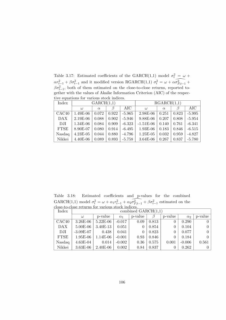
Table 3.17: Estimated coefficients of the GARCH(1,1) model σ2t = ω +
αr2t−1 + βσ2t−1 and it modified version RGARCH(1,1) σ2t = ω + ασ2P,t−1 +
βσ2t−1, both of them estimated on the close-to-close returns, reported to-gether with the values of Akaike Information Criterion (AIC) of the respec-tive equations for various stock indices.
Index GARCH(1,1) RGARCH(1,1)ω α β AIC ω α β AIC
CAC40 1.49E-06 0.072 0.922 -5.965 2.98E-06 0.251 0.823 -5.995DAX 2.19E-06 0.088 0.902 -5.946 9.88E-06 0.207 0.808 -5.954DJI 1.34E-06 0.084 0.909 -6.323 -1.51E-06 0.140 0.761 -6.341
FTSE 8.90E-07 0.080 0.914 -6.495 1.93E-06 0.183 0.846 -6.515Nasdaq 4.23E-05 0.044 0.880 -4.796 1.25E-05 0.032 0.959 -4.827Nikkei 4.40E-06 0.089 0.893 -5.758 3.64E-06 0.267 0.837 -5.780
Table 3.18: Estimated coefficients and p-values for the combined
GARCH(1,1) model σ2t = ω + α1r2t−1 + α2σ2P,t−1 + βσ2t−1 estimated on the
close-to-close returns for various stock indices.Index combined GARCH(1,1)
ω p-value α1 p-value β p-value α2 p-value
CAC40 3.26E-06 5.22E-06 -0.017 0.09 0.813 0 0.290 0DAX 5.00E-06 3.40E-13 0.051 0 0.854 0 0.104 0DJI -3.09E-07 0.438 0.041 0 0.823 0 0.077 0
FTSE 1.95E-06 1.14E-06 -0.001 0.93 0.846 0 0.184 0Nasdaq 4.63E-04 0.014 -0.002 0.36 0.575 0.001 -0.006 0.561Nikkei 3.63E-06 2.40E-06 0.002 0.84 0.837 0 0.262 0
106
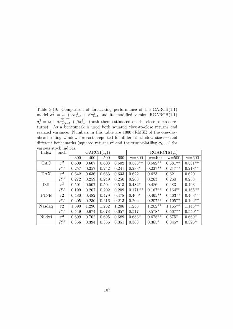
Table 3.19: Comparison of forecasting performance of the GARCH(1,1)model σ2t = ω + αr2t−1 + βσ2t−1 and its modified version RGARCH(1,1)
σ2t = ω + ασ2P,t−1 + βσ2t−1 (both them estimated on the close-to-close re-turns). As a benchmark is used both squared close-to-close returns andrealized variance. Numbers in this table are 1000×RMSE of the one-day-ahead rolling window forecasts reported for different window sizes w anddifferent benchmarks (squared returns r2 and the true volatility σtrue2) forvarious stock indices.
Index bnch GARCH(1,1) RGARCH(1,1)300 400 500 600 w=300 w=400 w=500 w=600
CAC r2 0.609 0.607 0.603 0.602 0.583** 0.582** 0.581** 0.581**RV 0.257 0.257 0.242 0.241 0.233* 0.227** 0.217** 0.218**
DAX r2 0.642 0.636 0.633 0.633 0.622 0.623 0.621 0.620RV 0.272 0.259 0.249 0.250 0.263 0.263 0.260 0.258
DJI r2 0.501 0.507 0.504 0.513 0.482* 0.486 0.483 0.493RV 0.199 0.207 0.202 0.209 0.171** 0.167** 0.164** 0.165**
FTSE r2 0.480 0.482 0.479 0.478 0.466* 0.465** 0.463** 0.463**RV 0.205 0.230 0.216 0.213 0.202 0.207** 0.195** 0.192**
Nasdaq r2 1.390 1.290 1.232 1.206 1.253 1.202** 1.165** 1.145**RV 0.549 0.674 0.678 0.657 0.517 0.578* 0.567** 0.550**
Nikkei r2 0.699 0.702 0.695 0.689 0.683* 0.678** 0.675* 0.669*RV 0.356 0.394 0.366 0.351 0.363 0.365* 0.345* 0.326*
107

108
Bibliography
[1] Alizadeh, S., Brandt, M. W., and Diebold, F. X. (2002). ”Range-
based estimation of stochastic volatility models.” Journal of Finance,
57, 1047–1091.
[2] Andersen, T. G., Bollerslev, T., Christoffersen P. and Diebold F.X.,
(2006), ”Volatility and Correlation Forecasting,” in G. Elliot, C.W.J.
Granger and A. Timmermann (eds.), Handbook of Economic Forecast-
ing, Chapter 15, 777-878. Amsterdam: North-Holland.
[3] Bollerslev, Tim (1986). “Generalized Autoregressive Conditional Het-
eroscedasticity.” Journal of Econometrics 31, 307–327.
[4] Bollerslev, T., and Mikkelsen, H. O. (1996), “Modeling and Pricing
Long Memory in Stock Market Volatility,” Journal of Econometrics,
73, 151–184.
[5] Barndorff-Nielsen, O. E., Nicolato, E. and Shephard, N.G. (2002),
”Some recent developments in stochastic volatility modelling.” Quanti-
tative Finance 2: 11–23.
[6] Michael W. Brandt, Christopher S. Jones. (2006). ”Volatility forecast-
ing with Range-Based EGARCH models.” Journal of Business and Eco-
nomic Statistics, 24(4): 470-486.
109
[7] Broto, C. and Ruiz, E. (2004), ”Estimation methods for stochastic
volatility models: a survey.” Journal of Economic Surveys, 18: 613–
649.
[8] Chou, R.Y. (2005) ”Forecasting financial volatilities with extreme val-
ues: the conditional autoregressive range (CARR) model.” Journal of
Money, Credit and Banking 37(3): 561–582.
[9] Dacorogna, M. M., R. Gencay, U. A. Muller, R. B. Olsen, and O. V.
Pictet. (2001). An Introduction to High-Frequency Finance. San Diego:
Academic Press.
[10] Engle, Robert (1982). “Autoregressive Conditional Heteroscedasticity
with Estimates of the Variance of U.K. Inflation.” Econometrica 50,
987–1008.
[11] Engle, R.F. and A.J. Patton (2001), “What is a good volatility model?”
Quantitative Finance, 1, 234–254.
[12] Garman, Mark B. and Klass, Michael J., (1980), ”On the Estimation of
Security Price Volatilities from Historical Data”, The Journal of Busi-
ness, Vol. 53, No. 1, 67-7
[13] Glosten, L. R., R. Jagannathan, and D. E. Runkle, 1993, ”On the
Relation Between the Expected Value and the Volatility of the Nominal
Excess Returns of Stocks,” Journal of Finance, 48, 1779-1801.
[14] Ghysels, E., Harvey, A. C. and Renault, E. (1996), ”Stochastic volatil-
ity”, in C. R. Rao and G. S. Maddala (eds.), Statistical Methods in
Finance (Amsterdam: North-Holland), 119-191.
110
[15] Hansen, P. R., and A. Lunde. (2005). “A Forecast Comparison of
Volatility Models: Does Anything Beat a GARCH (1,1)?”, Journal of
Applied Econometrics 20: 873–889
[16] Hansen, P. R., and A. Lunde. (2006). Consistent ranking of volatility
models, Journal Econometrics 131: 96–121.
[17] Hull, J. and White, A. (1987), ”The pricing of options on assets with
stochastic volatilities”, Journal of Finance, 42, 281-300.
[18] Kim, S., Shephard, N. and Chib, S. (1998). ”Stochastic volatility: like-
lihood inference and comparison with ARCH models.” Review of Eco-
nomic Studies 45: 361–393.
[19] Meilijson, I., (2009), ”The Garman–Klass volatil-
ity estimator revisited”, working paper available at:
http://arxiv.org/PS cache/arxiv/pdf/0807/0807.3492v2.pdf
[20] Melino, A. and S. Turnbull (1990). ”Pricing Foreign Currency Options
with Stochastic Volatility,” Journal of Econometrics, 45, 239-266.
[21] Molnar, P. (2011). ”Properties of Range-Based Volatility Estimators”,
working paper
[22] Nelson, D.B., 1990a, ”ARCH models as diffusion approximations”,
Journal of Econometrics 45, 7-39.
[23] Nelson, Daniel B., 1991, ”Conditional heteroskedasticity in asset pric-
ing: A new approach”, Econometrica 59, 347-370.
[24] Nelson, D. B. (1992), ”Filtering and Forecasting with Misspecified
ARCH Models I: Getting the Right Variance with the Wrong Model”,
Journal of Econometrics 2, 5 , 61-90.
111
[25] Parkinson, M. (1980). ”The extreme value method for estimating the
variance of the rate of return.” Journal of Business, 53, 61–65.
[26] Andrew J. Patton (2011), Volatility forecast comparison using imper-
fect volatility proxies, Journal of Econometrics, Volume 160, Issue 1,
Pages 246-256
[27] Poon, Ser-Huang and Clive W. Granger (2003), ”Forecasting Volatility
in Financial Markets: a Review”, Journal of Economic Literature, Vol.
41 (June 2003), pp. 478–539
[28] Shephard, N. (1996), ”Statistical aspects of ARCH and stochastic
volatility”, in D. R. Cox, 0. E. Barndorff-Nielson and D. V. Hinkley
(eds.), Time Series Models in Econometrics, Finance and Other Fields
(London: Chapman & Hall), 1-67.
[29] Shephard, N. and K. K. Shephard (2010), ”Realising the future: fore-
casting with high frequency based volatility (HEAVY) models”, Journal
of Applied Econometrics, 25 (2), pages 197–231.
[30] Taylor, S.J. (1986), Modeling Financial Time Series. Chichester, UK:
John Wiley and Sons.
112
4Tax-Adjusted Discount Rates: A General
Formula under Constant Leverage Ratios
Joint with Kjell G. Nyborg
113
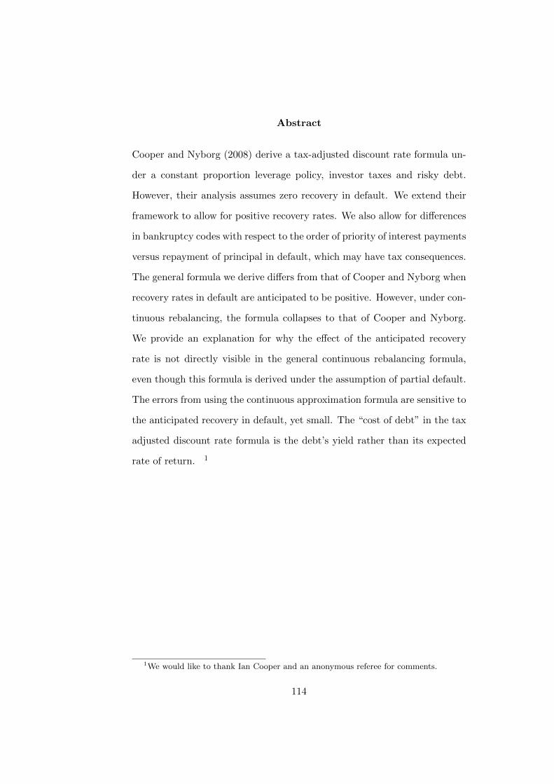
Abstract
Cooper and Nyborg (2008) derive a tax-adjusted discount rate formula un-
der a constant proportion leverage policy, investor taxes and risky debt.
However, their analysis assumes zero recovery in default. We extend their
framework to allow for positive recovery rates. We also allow for differences
in bankruptcy codes with respect to the order of priority of interest payments
versus repayment of principal in default, which may have tax consequences.
The general formula we derive differs from that of Cooper and Nyborg when
recovery rates in default are anticipated to be positive. However, under con-
tinuous rebalancing, the formula collapses to that of Cooper and Nyborg.
We provide an explanation for why the effect of the anticipated recovery
rate is not directly visible in the general continuous rebalancing formula,
even though this formula is derived under the assumption of partial default.
The errors from using the continuous approximation formula are sensitive to
the anticipated recovery in default, yet small. The “cost of debt” in the tax
adjusted discount rate formula is the debt’s yield rather than its expected
rate of return. 1
1We would like to thank Ian Cooper and an anonymous referee for comments.
114
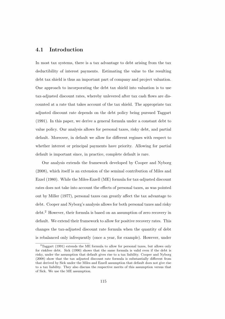
4.1 Introduction
In most tax systems, there is a tax advantage to debt arising from the tax
deductibility of interest payments. Estimating the value to the resulting
debt tax shield is thus an important part of company and project valuation.
One approach to incorporating the debt tax shield into valuation is to use
tax-adjusted discount rates, whereby unlevered after tax cash flows are dis-
counted at a rate that takes account of the tax shield. The appropriate tax
adjusted discount rate depends on the debt policy being pursued Taggart
(1991). In this paper, we derive a general formula under a constant debt to
value policy. Our analysis allows for personal taxes, risky debt, and partial
default. Moreover, in default we allow for different regimes with respect to
whether interest or principal payments have priority. Allowing for partial
default is important since, in practice, complete default is rare.
Our analysis extends the framework developed by Cooper and Nyborg
(2008), which itself is an extension of the seminal contribution of Miles and
Ezzel (1980). While the Miles-Ezzell (ME) formula for tax-adjusted discount
rates does not take into account the effects of personal taxes, as was pointed
out by Miller (1977), personal taxes can greatly affect the tax advantage to
debt. Cooper and Nyborg’s analysis allows for both personal taxes and risky
debt.2 However, their formula is based on an assumption of zero recovery in
default. We extend their framework to allow for positive recovery rates. This
changes the tax-adjusted discount rate formula when the quantity of debt
is rebalanced only infrequently (once a year, for example). However, under
2Taggart (1991) extends the ME formula to allow for personal taxes, but allows onlyfor riskfree debt. Sick (1990) shows that the same formula is valid even if the debt isrisky, under the assumption that default gives rise to a tax liability. Cooper and Nyborg(2008) show that the tax adjusted discount rate formula is substantially different fromthat derived by Sick under the Miles and Ezzell assumption that default does not give riseto a tax liability. They also discuss the respective merits of this assumption versus thatof Sick. We use the ME assumption.
115
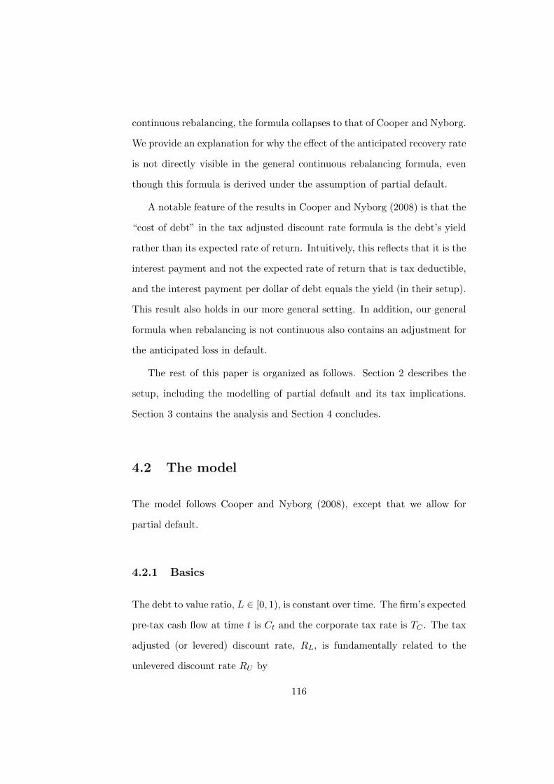
continuous rebalancing, the formula collapses to that of Cooper and Nyborg.
We provide an explanation for why the effect of the anticipated recovery rate
is not directly visible in the general continuous rebalancing formula, even
though this formula is derived under the assumption of partial default.
A notable feature of the results in Cooper and Nyborg (2008) is that the
“cost of debt” in the tax adjusted discount rate formula is the debt’s yield
rather than its expected rate of return. Intuitively, this reflects that it is the
interest payment and not the expected rate of return that is tax deductible,
and the interest payment per dollar of debt equals the yield (in their setup).
This result also holds in our more general setting. In addition, our general
formula when rebalancing is not continuous also contains an adjustment for
the anticipated loss in default.
The rest of this paper is organized as follows. Section 2 describes the
setup, including the modelling of partial default and its tax implications.
Section 3 contains the analysis and Section 4 concludes.
4.2 The model
The model follows Cooper and Nyborg (2008), except that we allow for
partial default.
4.2.1 Basics
The debt to value ratio, L ∈ [0, 1), is constant over time. The firm’s expected
pre-tax cash flow at time t is Ct and the corporate tax rate is TC . The tax
adjusted (or levered) discount rate, RL, is fundamentally related to the
unlevered discount rate RU by
116
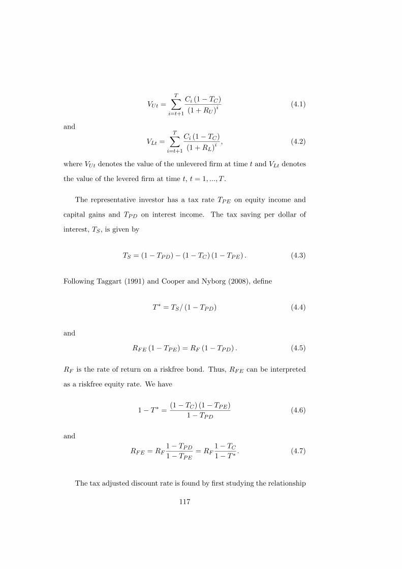
VUt =T∑
i=t+1
Ci (1− TC)
(1 +RU )i(4.1)
and
VLt =
T∑i=t+1
Ci (1− TC)
(1 +RL)i, (4.2)
where VUt denotes the value of the unlevered firm at time t and VLt denotes
the value of the levered firm at time t, t = 1, ..., T .
The representative investor has a tax rate TPE on equity income and
capital gains and TPD on interest income. The tax saving per dollar of
interest, TS , is given by
TS = (1− TPD)− (1− TC) (1− TPE) . (4.3)
Following Taggart (1991) and Cooper and Nyborg (2008), define
T ∗ = TS/ (1− TPD) (4.4)
and
RFE (1− TPE) = RF (1− TPD) . (4.5)
RF is the rate of return on a riskfree bond. Thus, RFE can be interpreted
as a riskfree equity rate. We have
1− T ∗ =(1− TC) (1− TPE)
1− TPD(4.6)
and
RFE = RF1− TPD1− TPE
= RF1− TC1− T ∗
. (4.7)
The tax adjusted discount rate is found by first studying the relationship
117
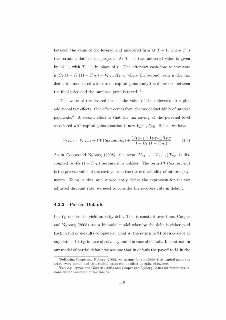
between the value of the levered and unlevered firm at T − 1, where T is
the terminal date of the project. At T − 1 the unlevered value is given
by (4.1), with T − 1 in place of t. The after-tax cash-flow to investors
is CT (1− TC) (1− TPE) + VUT−1TPE , where the second term is the tax
deduction associated with tax on capital gains (only the difference between
the final price and the purchase price is taxed).3
The value of the levered firm is the value of the unlevered firm plus
additional tax effects. One effect comes from the tax deductibility of interest
payments.4 A second effect is that the tax saving at the personal level
associated with capital gains taxation is now VLT−1TPE . Hence, we have
VLT−1 = VUT−1 + PV (tax saving) +(VLT−1 − VUT−1)TPE
1 +RF (1− TPD). (4.8)
As in Cooperand Nyborg (2008), the term (VLT−1 − VUT−1)TPE is dis-
counted by RF (1− TPD) because it is riskless. The term PV (tax saving)
is the present value of tax savings from the tax deductibility of interest pay-
ments. To value this, and subsequently derive the expression for the tax
adjusted discount rate, we need to consider the recovery rate in default.
4.2.2 Partial Default
Let YD denote the yield on risky debt. This is constant over time. Cooper
and Nyborg (2008) use a binomial model whereby the debt is either paid
back in full or defaults completely. That is, the return to $1 of risky debt at
any date is 1+YD in case of solvency and 0 in case of default. In contrast, in
our model of partial default we assume that in default the payoff to $1 in the
3Following Cooperand Nyborg (2008), we assume for simplicity that capital gains taxarises every period and that capital losses can be offset by gains elsewhere.
4See, e.g., Arzac and Glosten (2005) and Cooper and Nyborg (2006) for recent discus-sions on the valuation of tax shields.
118
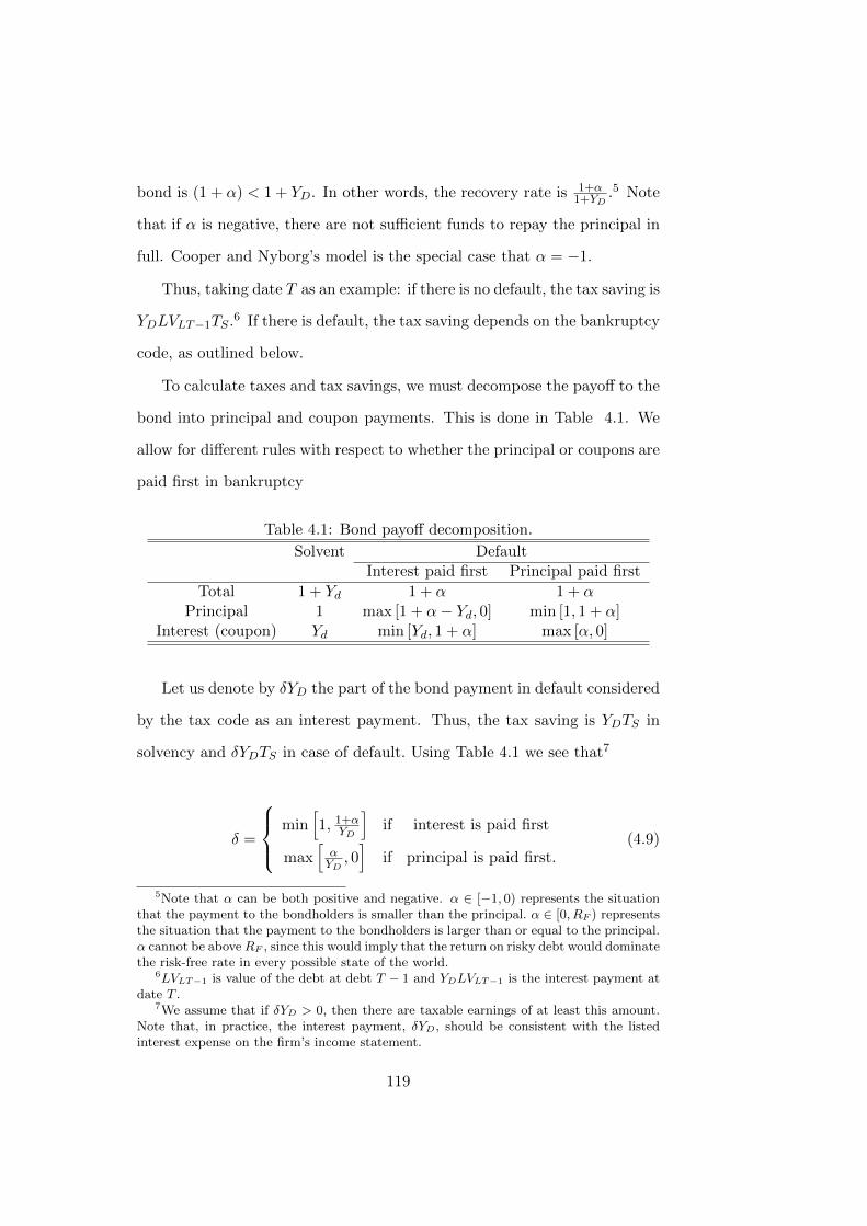
bond is (1 + α) < 1 + YD. In other words, the recovery rate is 1+α1+YD
.5 Note
that if α is negative, there are not sufficient funds to repay the principal in
full. Cooper and Nyborg’s model is the special case that α = −1.
Thus, taking date T as an example: if there is no default, the tax saving is
YDLVLT−1TS .6 If there is default, the tax saving depends on the bankruptcy
code, as outlined below.
To calculate taxes and tax savings, we must decompose the payoff to the
bond into principal and coupon payments. This is done in Table 4.1. We
allow for different rules with respect to whether the principal or coupons are
paid first in bankruptcy
Table 4.1: Bond payoff decomposition.
Solvent DefaultInterest paid first Principal paid first
Total 1 + Yd 1 + α 1 + αPrincipal 1 max [1 + α− Yd, 0] min [1, 1 + α]
Interest (coupon) Yd min [Yd, 1 + α] max [α, 0]
Let us denote by δYD the part of the bond payment in default considered
by the tax code as an interest payment. Thus, the tax saving is YDTS in
solvency and δYDTS in case of default. Using Table 4.1 we see that7
δ =
min[1, 1+αYD
]if interest is paid first
max[αYD, 0]
if principal is paid first.(4.9)
5Note that α can be both positive and negative. α ∈ [−1, 0) represents the situationthat the payment to the bondholders is smaller than the principal. α ∈ [0, RF ) representsthe situation that the payment to the bondholders is larger than or equal to the principal.α cannot be aboveRF , since this would imply that the return on risky debt would dominatethe risk-free rate in every possible state of the world.
6LVLT−1 is value of the debt at debt T − 1 and YDLVLT−1 is the interest payment atdate T .
7We assume that if δYD > 0, then there are taxable earnings of at least this amount.Note that, in practice, the interest payment, δYD, should be consistent with the listedinterest expense on the firm’s income statement.
119
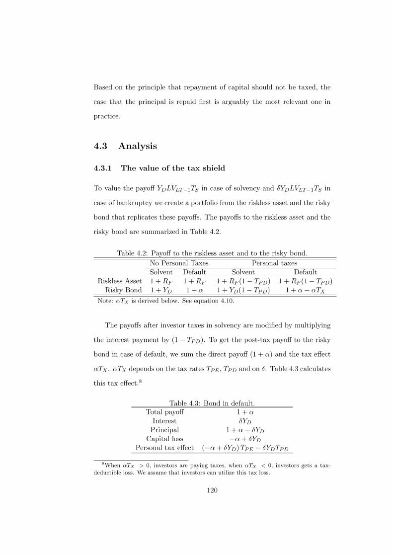
Based on the principle that repayment of capital should not be taxed, the
case that the principal is repaid first is arguably the most relevant one in
practice.
4.3 Analysis
4.3.1 The value of the tax shield
To value the payoff YDLVLT−1TS in case of solvency and δYDLVLT−1TS in
case of bankruptcy we create a portfolio from the riskless asset and the risky
bond that replicates these payoffs. The payoffs to the riskless asset and the
risky bond are summarized in Table 4.2.
Table 4.2: Payoff to the riskless asset and to the risky bond.
No Personal Taxes Personal taxesSolvent Default Solvent Default
Riskless Asset 1 +RF 1 +RF 1 +RF (1− TPD) 1 +RF (1− TPD)Risky Bond 1 + YD 1 + α 1 + YD(1− TPD) 1 + α− αTX
Note: αTX is derived below. See equation 4.10.
The payoffs after investor taxes in solvency are modified by multiplying
the interest payment by (1− TPD). To get the post-tax payoff to the risky
bond in case of default, we sum the direct payoff (1 + α) and the tax effect
αTX . αTX depends on the tax rates TPE , TPD and on δ. Table 4.3 calculates
this tax effect.8
Table 4.3: Bond in default.Total payoff 1 + α
Interest δYDPrincipal 1 + α− δYD
Capital loss −α+ δYDPersonal tax effect (−α+ δYD)TPE − δYDTPD
8When αTX > 0, investors are paying taxes, when αTX < 0, investors gets a tax-deductible loss. We assume that investors can utilize this tax loss.
120
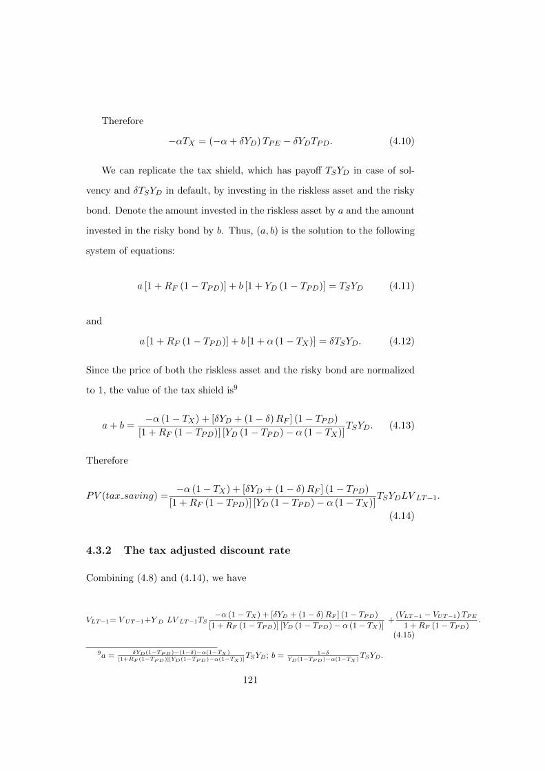
Therefore
−αTX = (−α+ δYD)TPE − δYDTPD. (4.10)
We can replicate the tax shield, which has payoff TSYD in case of sol-
vency and δTSYD in default, by investing in the riskless asset and the risky
bond. Denote the amount invested in the riskless asset by a and the amount
invested in the risky bond by b. Thus, (a, b) is the solution to the following
system of equations:
a [1 +RF (1− TPD)] + b [1 + YD (1− TPD)] = TSYD (4.11)
and
a [1 +RF (1− TPD)] + b [1 + α (1− TX)] = δTSYD. (4.12)
Since the price of both the riskless asset and the risky bond are normalized
to 1, the value of the tax shield is9
a+ b =−α (1− TX) + [δYD + (1− δ)RF ] (1− TPD)
[1 +RF (1− TPD)] [YD (1− TPD)− α (1− TX)]TSYD. (4.13)
Therefore
PV (tax saving) =−α (1− TX) + [δYD + (1− δ)RF ] (1− TPD)
[1 +RF (1− TPD)] [YD (1− TPD)− α (1− TX)]TSYDLV LT−1.
(4.14)
4.3.2 The tax adjusted discount rate
Combining (4.8) and (4.14), we have
VLT−1= V UT−1+Y D LV LT−1TS−α (1− TX) + [δYD + (1− δ)RF ] (1− TPD)
[1 +RF (1− TPD)] [YD (1− TPD)− α (1− TX)]+
(VLT−1 − VUT−1)TPE1 +RF (1− TPD)
.
(4.15)
9a = δYD(1−TPD)−(1−δ)−α(1−TX )[1+RF (1−TPD)][YD(1−TPD)−α(1−TX )]
TSYD; b = 1−δYD(1−TPD)−α(1−TX )
TSYD.
121
This can be rewritten using (4.3)-(4.7) as
VLT−1= V UT−1+LVLT−1T
∗YD (1− TC)
(1− T ∗) (1 +RFE)
[δYD + (1− δ)RF ] (1− TPD)− α (1− TX)
YD (1− TPD)− α (1− TX).
(4.16)
By (4.1) and (4.2),
VUT−1 = VLT−11 +RL1 +RU
. (4.17)
Thus, we obtain the relationship between RL and RU :
RL= RU− (1 +RU )LYDT
∗ (1− TC)
(1− T ∗) (1 +RFE)
[δYD + (1− δ)RF ] (1− TPD)− α (1− TX)
YD (1− TPD)− α (1− TX).
(4.18)
Substituting (4.10) into (4.18) yields
RL= RU−LYDT
∗ (1− TC)
1− T ∗1 +RU
1 +RFE
(1− δ)RF (1− TPD) + δYD (1− TPE)− α (1− TPE)
YD (1− TPD + δ (TPD − TPE))− α (1− TPE),
(4.19)
where δ is given by (4.9).
While we have derived RL by analyzing the model at time T − 1, the
same inductive argument as in Cooperand Nyborg (2008) can be used to
establish that RL as given by (4.19) holds at any date t. Thus, this is our
general tax adjusted discount rate, that takes account of risky debt, personal
taxes, and partial default.
The formula for the tax adjusted discount rate derived by Cooper and
Nyborg (2008) is:
RL = RU −LYDT
∗ (1− TC)
1− T ∗1 +RU
1 +RFE
1 +RF1 + YD
. (C&N 12)
As pointed out above, Cooper and Nyborg’s model corresponds to the special
122
case that α = −1 and therefore also δ = 0. However, substituting these
values into (4.19) yields:
RL= RU−LYDT
∗ (1− TC)
1− T ∗1 +RU
1 +RFE
(1− TPE) +RF (1− TPD)
(1− TPE) + YD (1− TPD), (4.20)
which is slightly different from (C&N 12). The reason for this difference
comes from the tax treatment of capital losses. In the case of complete
default, the investor suffers a capital loss of 1 per dollar invested in the bond.
This loss is tax deductible and therefore the total payoff to the investor is
1×TPE , assuming a capital gains of TPE . In contrast, Cooper and Nyborg’s
formula is derived under the assumption that the total payoff to the investor
here is 1× TPD.10
4.3.3 Continuous rebalancing
The rates of return in the analysis above may be interpreted as annual
returns, with rebalancing of the debt to the target leverage ratio carried out
once a year. In this subsection, we derive the general expression for the tax
adjusted discount rate under continuous rebalancing of the debt.
We start by dividing the year into n equal periods, with rebalancing
happening at the end of each period. The annually compounded rates RU
and RF are not affected by the frequency of rebalancing. Let
rU,n = (1 +Ru)1n − 1 (4.21)
be the unlevered discount rate over a period of length 1/n. Define rF,n and
10While we differ in this detail, both we and Cooper and Nyborg assume elsewhere thatcapital gains are taxed at TPE . In particular, Cooper and Nyborg (2008) use a capitalgains tax of TPE in their equation (A2), as do we in the corresponding expression in thispaper. Thus, (4.20) is arguably the more correct tax adjusted discount rate formula undercomplete default in the Cooper and Nyborg model.
123
rFE,n analogously.
We assume that the binomial process for the risky debt holds over each
period of length 1/n, with the per period yield being denoted by yD,n =
(1 + YD)1/n − 1.
For simplicity, we assume that the pre-tax payoff to the risky bond in
default, 1 +α, is unaffected by the length of a period. However, as a period
becomes arbitrarily small, the per period yield on the bond also becomes
small. Thus, to ensure a recovery rate below 1 for arbitrarily short periods,
we assume that 1 + α < 1, i.e., α < 0. This also means that when the
principal is viewed as being paid first in bankruptcy, δ = 0. We consider this
the most relevant case as it is consistent with the principle that repayment
of capital is not taxed. In the case that interest is paid first in bankruptcy,
δ may depend on n. Clearly, it is 0 if 1 + α = 0. If 1 + α > 0, there is
n′ such that for all n > n′, 1 + α > yD,n, since yD,n is decreasing in n and
converges to zero. Thus, for sufficiently large n, δ will be equal to 1 if the tax
code treats interest as being paid first in bankruptcy. In short, our model
collapses to either having δ = 0 or δ = 1.
Thus, using (4.19), the tax adjusted discount rate over a period of length
1/n is
rL,n = rU,n−LyD,nT
∗ (1− TC)
1− T ∗1 + rU,n
1 + rFE,n
(1− δ) rF,n (1− TPD) + δyD,n (1− TPE)− α (1− TPE)
yD,n (1− TPD + δ (TPD − TPE))− α (1− TPE).
(4.22)
Denote the third fraction on the right hand side by A. Multiplying both
sides by n, we have
nrL,n = nrU,n − nyD,nLT ∗ (1− TC)
1− T ∗
(1 + rU,n
1 + rFE,n
)×A. (4.23)
124
Now define RU,n = nrU,n, RL,n = nrL,nYD,n = nyD,n. These are the
annualized rates corresponding to rU,n, rL,n, and yD,n, respectively. By
definition, RU = limn→∞RU,n is the continuously compounded rate that
corresponds to RU . YD = limn→∞ YD,n is the continuously compounded
rate corresponding to YD. RL = limn→∞RL,n is the tax adjusted discount
rate under continuous rebalancing. RU , YD, and RL are continuously com-
pounded rates stated on a standard per annum basis.
Using these definitions in (4.23), we have
limn→∞
RL,n = limn→∞
{RU,n − YD,n
LT ∗ (1− TC)
1− T ∗
(1 + rU,n
1 + rFE,n
)×A
}(4.24)
which reduces to11
RL = RU − YDLT ∗1− TC1− T ∗
. (4.25)
Equation (4.25) thus provides us with the (continuously compounded) tax
adjusted discount rate under continuous rebalancing.
This is exactly the same formula as derived by Cooper and Nyborg
(2008), starting from (C&N 12). That partial default does not alter the
formula for the tax adjusted discount rate under continuous rebalancing is
surprising.
To see the intuition for this, recall that in the continuous rebalancing
model, we either have δ = 0 or δ = 1. If δ = 1, equation (4.22) reduces to
rL,n = rU,n −LyD,nT
∗ (1− TC)
1− T ∗1 + rU,n
1 + rFE,n. (4.26)
As seen, α has dropped out. This is intuitive, since δ = 1 means that the
interest tax shield is unaffected by the recovery in default.
11Since each of the last two terms converge to 1.
125
If δ = 0, the term A in (4.23) becomes
rF,n(1− TPD)− α(1− TPE)
yD,n(1− TPD)− α(1− TPE). (4.27)
This clearly converges to 1, implying that α drops out of the analysis. More
intuitively, when δ = 0, the recovery rate only affects the capital loss in
default and this gets squeezed towards zero over an arbitrarily short time
horizon since the implied probability of default must converge to zero.
To see this, note that in the basic discrete rebalancing model, it must be
true that
(1− p) (1 + YD) + p (1 + α) = 1 +RF , (4.28)
where p is the risk-neutral probability of default. When we rebalance more
frequently, to keep our model arbitrage-free, the risk-neutral probability of
default must adjust according to
pn =yD,n − rF,nyD,n − α
. (4.29)
Thus, the probability of default in a small interval approaches zero in the
limit.
The continuous rebalancing tax adjusted discount rate formula itself is
intuitive, especially when rewritten in the following form [using (4.3) and
(4.6)]:
RL = RU −YDLTS1− TPE
. (4.30)
This shows clearly that the tax adjusted discount rate is the unlevered dis-
count rate less the tax saving per dollar of firm value. The “raw” tax saving,
YDLTS , is grossed up by 1− TPE , reflecting that RL is a discount rate that
is applied to after-corporate-tax, but before-personal-tax, unlevered cash
126
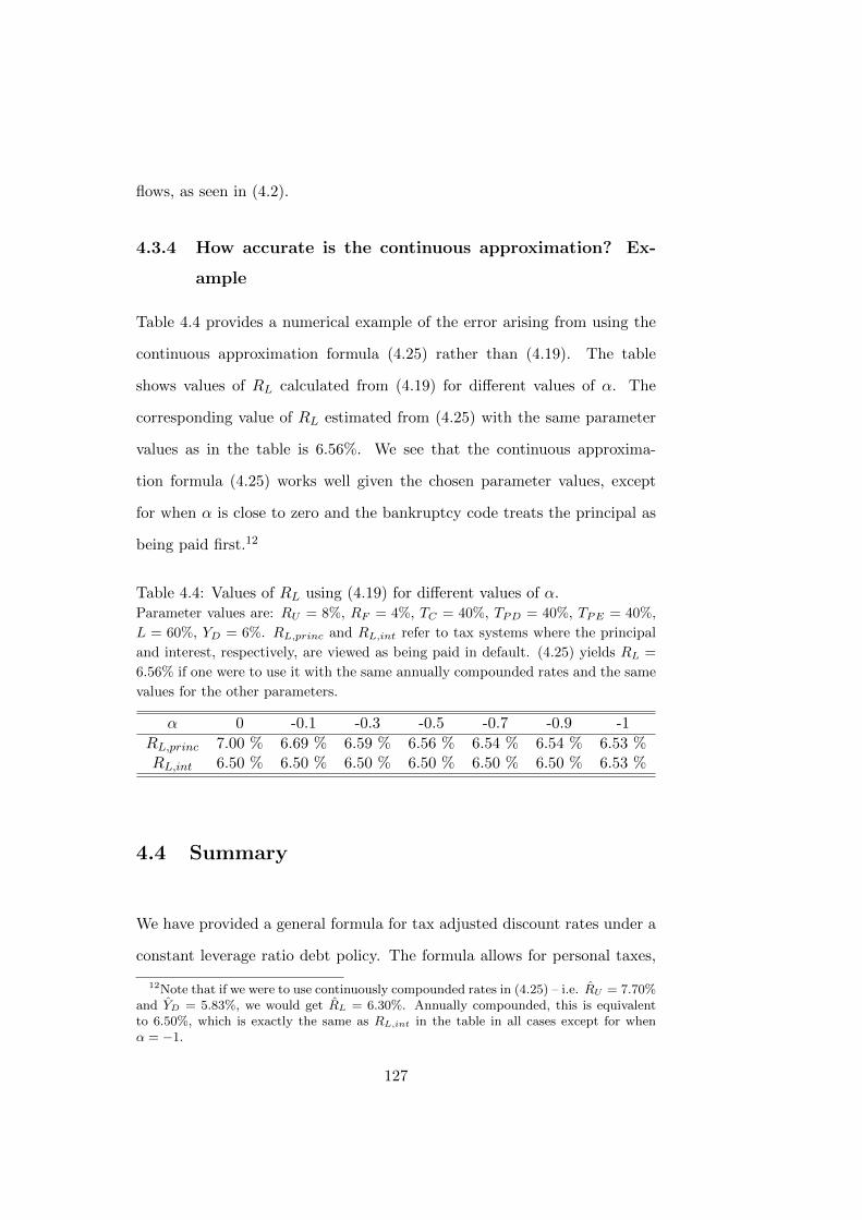
flows, as seen in (4.2).
4.3.4 How accurate is the continuous approximation? Ex-
ample
Table 4.4 provides a numerical example of the error arising from using the
continuous approximation formula (4.25) rather than (4.19). The table
shows values of RL calculated from (4.19) for different values of α. The
corresponding value of RL estimated from (4.25) with the same parameter
values as in the table is 6.56%. We see that the continuous approxima-
tion formula (4.25) works well given the chosen parameter values, except
for when α is close to zero and the bankruptcy code treats the principal as
being paid first.12
Table 4.4: Values of RL using (4.19) for different values of α.Parameter values are: RU = 8%, RF = 4%, TC = 40%, TPD = 40%, TPE = 40%,
L = 60%, YD = 6%. RL,princ and RL,int refer to tax systems where the principal
and interest, respectively, are viewed as being paid in default. (4.25) yields RL =
6.56% if one were to use it with the same annually compounded rates and the same
values for the other parameters.
α 0 -0.1 -0.3 -0.5 -0.7 -0.9 -1
RL,princ 7.00 % 6.69 % 6.59 % 6.56 % 6.54 % 6.54 % 6.53 %RL,int 6.50 % 6.50 % 6.50 % 6.50 % 6.50 % 6.50 % 6.53 %
4.4 Summary
We have provided a general formula for tax adjusted discount rates under a
constant leverage ratio debt policy. The formula allows for personal taxes,
12Note that if we were to use continuously compounded rates in (4.25) – i.e. RU = 7.70%and YD = 5.83%, we would get RL = 6.30%. Annually compounded, this is equivalentto 6.50%, which is exactly the same as RL,int in the table in all cases except for whenα = −1.
127
risky debt, and partial default. It also handles different rules with respect
to the order of priority of interest payments versus repayment of principal
in default. In doing this, we have expanded on the analysis of Cooper and
Nyborg (2008), who assumed complete default (zero recovery in default).
This is important because recovery rates in practice typically are signifi-
cantly larger than zero. Our general formula differs from that of Cooper
and Nyborg because recovery rates affect the tax adjusted discount rate.
We have also shown that the effect of nonzero recovery rates can be quite
small, and if debt rebalancing is continuous, the effect disappears altogether.
Our analysis thus shows that Cooper and Nyborg’s tax adjusted discount
rate formula under continuous rebalancing holds under more general condi-
tions than those under which it was originally derived. We have provided an
intuition for why this is so. The usefulness of the continuous approximation
formula is that it is easy to use and does not require estimates of recovery
rates in default. In the context of a numerical example, we have illustrated
that the errors from using it are quite small, even for large recovery rates.
128
Bibliography
[1] Arzac, E.R. and L.R. Glosten, 2005, A Reconsideration of Tax Shield
Valuation, European Financial Management, 11, 453–461.
[2] Cooper, I.A. and K.G. Nyborg, 2006, The Value of Tax Shields IS Equal
to the Present Value of Tax Shields, Journal of Financial Economics,
81, 215–225.
[3] Cooper, I.A. and K.G. Nyborg, 2008, Tax-Adjusted Discount Rates With
Investor Taxes and Risky Debt, Financial Management, Summer 2008,
365–379
[4] Miles, J. and J.R. Ezzell, 1980, The Weighted Average Cost of Capital,
Perfect Capital Markets and Project Life: A Clarification, Journal of
Financial and Quantitative Analysis, 15 (3), 719–730.
[5] Miller, M.H., 1977, Debt and Taxes, Journal of Finance, 32, 261–276.
[6] Sick, G.A., 1990, Tax-Adjusted Discount Rates, Management Science,
36 (12), 1432–1450.
[7] Taggart, R.A., 1991, Consistent Valuation and Cost of Capital Expres-
sions with Corporate and Personal Taxes, Financial Management, (Au-
tumn), 8–20.
129