Embed Size (px)
Citation preview
ESPlannerTM
-- A Revolution in Financial Planning
Tutorial
Economic Security Planning, Inc.’s website is www.ESPlanner.com.
Copyright© Economic Security Planning, Inc., 1999, 2000, 2001, 2002, 2003, 2005
U.S. Patent No. 6,611,807. Visit www.ESPlanner.com for to purchase annual updates!
Send email to [email protected] for customer support.
ESPlanner and EsplannerPlus are trademarks of Economic Security Planning, Inc. Economic Security Planning, Inc. gratefully acknowledges research support provided by the National Institute of Aging via a Small Technology Transfer Grant.

1
Contents
1. Introduction
2. Learning Tools
3. Customer Support
4. Warranty Disclaimer and Permitted Scope of Use
5. Overview of the Software
6. Customizing Your Reports
7. Activating Contingent Planning and Monte Carlo Simulations
8. Optimizing Your Family’s Plan
9. Monte Carlo Simulations
10. Borrowing Constraints
11. Getting Started
12. Joe and Sally
a. Entering Earnings
b. Entering Special Expenses
c. Entering Estate Plans and Current Life Insurance Holdings d. Entering Regular Assets
e. Entering Actual Current Saving
f. Entering Housing g. Entering Social Security Benefit Collection Dates and Covered Earnings
h. Entering Demographic, Economic, Tax, and Benefit Assumptions
i. Generating their Plan j. Current Recommendations
k. Annual Recommendations
l. Spending Report m. Regular Assets Report
n. Total Income Report
o. Net Worth Report p. Detailed Reports
q. Survivor Reports
r. Budgeting Module
13. Joe Retires Early
14. Joe and Sally Do Contingent Planning
15. Joe and Sally Accumulate a Reserve Fund
16. The Whitneys Have Retirement Accounts
17. Joe and Sally Receive a Big Inheritance
18. Joe and Sally Downsize and Retire in Florida
19. Joe and Sally Run Monte Carlo

2
Introduction
Thank you for purchasing ESPlanner. a unique patented financial planning software package based on the
life-cycle model of saving. The life-cycle model, developed by Nobel Laureate Franco Modigliani, is the
standard framework used by economists to understand consumption, saving, and insurance behavior. The
model is grounded in the common-sense notion that households seek to achieve and maintain the highest
possible living standard through time. Economists refer to the desire to avoid abrupt changes over time in
one’s living standard as consumption smoothing.
ESPlanner recommends annual levels of consumption, saving, and life insurance holdings to achieve
consumption smoothing. Specifically, given its inputs, the program’s recommendations maintain your
family’s living standard at the highest affordable level and guarantee potential survivors that same living
standard. Solving the problem of both maximizing and smoothing your household’s living standard over
time and across survival contingencies is not easy. ESPlanner uses a patented dynamic programming
method to solve this problem. Dynamic programming is an advanced mathematical technique that has not
been used in previous commercial financial planning applications.
In providing its basic recommendations for how much your family should consume, save, and insure each
year, ESPlanner considers how much your regular and retirement account assets will yield, each year.
ESPlannerPlus incorporates all the features of ESPlanner, but it also recognizes that future rates of return are
uncertain. Its Monte Carlo simulations show the annual variability of your family’s living standard and
other economic variable arising from the household’s asset allocation decisions.
Our approach to financial planning differs markedly from conventional financial planning. Conventional
planning makes you plan for yourself by making you specify retirement spending targets. This is very
difficult and can be dangerous. If you set your target too low, you’ll be advised to under save and
underinsure and your family’s living standard will drop, if not plunge, at retirement. If you set your target
too high, you’ll be advised to over save and over insure and your family’s living standard will jump up, if
not soar, at retirement. In either case, there’s an abrupt change in living standard – precisely the opposite
of consumption smoothing.
Rather than asking you to find future spending targets that are consistent with lifetime consumption
smoothing, ESPlanner finds the right targets automatically by determining your household’s highest
sustainable living standard along with the savings and amount of life insurance needed to preserve that
living standard through time. These calculations are made taking into account the taxes you will pay in
each future year and the borrowing limitations you face.
ESPlanner recommends annual levels of consumption, saving, and life insurance holdings. Consumption
refers here to all living expenses apart from housing expenses, special expenditures, contributions to a
reserve fund, taxes, contributions to retirement accounts, and life insurance premium payments, all of which
are treated as “off-the-top” expenditures that have to be made when they come due. Annual consumption

3
recommendations are adjusted for the household composition in the year in question; i.e., when children
are young and still in the household, the program recommends higher consumption expenditures. In so
doing, the program takes into account the fact that two can live more cheaply than one and that children
may be less or more expensive to support than adults.
Another key feature of ESPlanner is contingent planning. Contingent planning permits you to plan in
detail for the possible early deaths of your family’s earners. Specifically, it allows you to specify how your
family’s earnings, special expenditures, special receipts, retirement plans, dates of Social Security
retirement benefit collection, and contributions to retirement accounts would differ were a spouse/partner to
die. ESPlanner provides easy ways of inputting these data when one’s contingent and regular amounts are
identical. ESPlanner defaults to the household’s regular amounts for these expenditures, but permits you
to override the defaults as necessary.
You can activate contingent planning using the Family Information screen. ESPlannerPlus’ Monte-Carlo
simulations allow you to construct ten different portfolios (combinations of financial assets), which your
family might want to hold in the future. You can then specify for each future year which of these ten
portfolios will apply to your family members’ regular assets and retirement account assets. When you run
the program’s Monte-Carlo reports, it generates a variety of tables and charts that display the variability of
your family’s living standard, income, and assets over time given the portfolios your family intends to
hold now and in the future. If you purchased ESPlannerPlus, you can also activate the Monte Carlo
simulations on the Family Information screen.
Unlike the other reports, which run in a matter of seconds on a fast machine, the Monte Carlo
calculations involve very extensive and time-consuming calculations. Indeed, for young families,
generating the Monte Carlo reports can take several minutes even on today’s most advanced
desktops. If your computer is not very fast and has limited memory, you will need to be patient.
On the other hand, if you just want to run the main, detailed, or survivor reports, you can deactivate the
Monte Carlo simulations on the Family Information Screen.
A hallmark of ESPlanner is the precision with which it calculates annual federal and state income taxes,
FICA taxes, and social security benefits. Even small mistakes in determining a household’s future taxes
and benefits can lead to major mistakes in current saving and insurance recommendations because they are
generally repeated for a large number of future years, making their aggregate effect sizable.
In ESPlanner all taxes and Social Security benefits are calculated separately for each year the household
head and spouse/partner could both be alive and for each year that the household head and spouse/partner
could be widowed. In the latter case, ESPlanner calculates taxes and benefits conditional on the age of
death of the decedent. In the case of partners – unmarried couples – the program calculates taxes treating
each partner as a single tax payer.

4
The amount of taxes a household pays over time depends on how much it earns and how much asset
income it receives. The amount of asset income depends, in turn, on the amount of assets, which depends
on decisions about spending and saving. Hence, one can’t determine how much in taxes a household will
pay over time without knowing how much it will spend over time. But one can’t determine a household’s
spending over time without knowing its taxes over time.
If taxes depend on spending, but spending depends on taxes, how can we resolve this chicken and egg
problem, which economists call a simultaneity problem? The answer is by developing iterative algorithms
that simultaneously determine how much is spent and how much taxes are paid over the household’s entire
life cycle, include the life cycles of survivors conditional, in the case of couples, on all the possible different
dates of death of spouses and partners.
As part of these algorithms, the program’s federal income tax calculator decides if the household should
itemize deductions, whether it is eligibility for the earned-income and child-tax credits, and the extent to
which its Social Security benefits are subject to taxation. It also includes the Alternative Minimum Tax.
And it takes into account the most recent changes in federal and state income tax provisions. The state
income tax calculator incorporates the progressive rate structure, deductions, and exemptions in each state’s
income tax law.
As indicated, ESPlanner lets households declare themselves as partnered, in which case the software
calculates federal and state income taxes for each partner separately using singles or head of household tax
tables and provisions. This is a very important feature given the large number of unmarried couples in
American society.
The program’s Social Security benefit calculator determines retirement, spousal, survivor, divorcee, child,
and mother and father benefits subject to the remaining earnings test, benefit-re-computation provisions,
delayed retirement credits, early retirement reduction factors, increases in the age of normal retirement
scheduled by law, maximum family benefits, etc. Since the amounts of survivor and child, mother, and
father benefits depend on the precise earnings history of the deceased spouse, ESPlanner calculates these
benefits separately conditional on each and every possible date of death of each spouse. ESPlanner also
applies special formulae for calculating the benefits of government employees who receive pensions based
on non-Social Security covered employment.
Given the complex nature of the calculations needed to achieve a consumption-smoothing financial plan, a
natural question to ask is whether one can really tell if ESPlanner is making the correct calculations. The
answer is yes. First, one can immediately verify that the program’s recommendations never put the
household in debt or in more debt than the household is willing to incur. Second, one can easily check
that the household’s living standard is being smoothed. Third, one can readily verify that the program’s
recommended life insurance holdings are, to the dollar, what is needed to preserve survivors’ living
standards. And fourth, one can see from the software’s reports that all the inputs, such as housing

5
expenses, bequests, contributions to reserve funds, and special expenditures, are being included in the
program.
The only thing users can’t immediately verify is the program’s calculation of taxes and Social Security
benefits. These are the only variables shown in the reports not directly inputted by users. But, as just
indicated, taxes and Social Security benefits are calculated with great care.
ESPlanner was developed by Professor Laurence J. Kotlikoff, Chairman of the Department of Economics at
Boston University and Dr. Jagadeesh Gokhale, a Senior Fellow at the Cato Institution, who served for
many years as Senior Academic Advisor to the Federal Reserve Bank of Cleveland. The two economists
are leading authorities on the economics of consumption, saving, insurance, portfolio choice, and fiscal
policy.
The program took a decade to develop and is used routinely for research, results of which are posted at
www.esplanner.com. Much of this research was supported by Boston University, the National Institute of
Aging (an institute of the National Institutes of Health), the Smith-Richardson Foundation, and TIAA-
CREF, for which we are most grateful. The National Institute of Aging also provided critical and early
support for research on this product via a STTR grant.
6
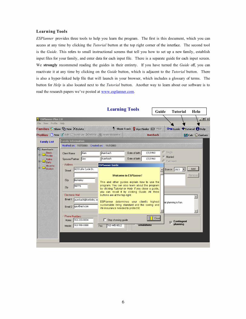
Learning Tools
ESPlanner provides three tools to help you learn the program. The first is this document, which you can
access at any time by clicking the Tutorial button at the top right corner of the interface. The second tool
is the Guide. This refers to small instructional screens that tell you how to set up a new family, establish
input files for your family, and enter data for each input file. There is a separate guide for each input screen.
We strongly recommend reading the guides in their entirety. If you have turned the Guide off, you can
reactivate it at any time by clicking on the Guide button, which is adjacent to the Tutorial button. There
is also a hyper-linked help file that will launch in your browser, which includes a glossary of terms. The
button for Help is also located next to the Tutorial button. Another way to learn about our software is to
read the research papers we’ve posted at www.esplanner.com.
Learning Tools
Guide Tutorial Help

7
Customer Support
Economic Security Planning, Inc. prides itself on providing fast customer support. If you have questions
or technical problems, please email us at [email protected]. Please include your phone number in case
we want to call you.

8
Warranty Disclaimer and Permitted Scope of Use
ESPLANNER’S AND ESPLANNERPLUS’ RECOMMENDATIONS DO NOT CONSTITUTE
FINANCIAL ADVICE ESPLANNER’S CREATORS ARE NOT CERTIFIED, REGISTERED, AUTHORIZED, OR ANY OTHER FORM OF FINANCIAL PLANNERS. ECONOMIC SECURITY PLANNING, INC. DOES NOT GUARANTEE THAT ESPLANNER’S RECOMMENDATIONS WILL NECESSARILY ACHIEVE A SECURE ECONOMIC PLAN. LIKE ANY SOFTWARE PRODUCT, ESPLANNER MAY HAVE ERRORS IN ITS UNDERLYING CODE. AND THE ASSUMPTIONS ABOUT THE FUTURE THAT IT MAKES AND THAT USERS INPUT MAY PROVE FALSE. ESPLANNER IS A TOOL FOR HELPING YOU THINK THROUGH YOUR ECONOMIC FUTURES. ITS “RECOMMENDATIONS” SHOULD BE VIEWED AS SUGGESTIVE AND INFORMATIVE INPUTS INTO YOUR DECISION-MAKING WITH RESPECT TO SAVING AND THE PURCHASE OF LIFE INSURANCE. ESPLANNER IS NEITHER ECONOMIC NOR FINANCIAL GOSPEL. IT ALSO EXCLUDES A NUMBER OF FACTORS, SUCH AS THE UNCERTAINTY OF FUTURE INCOME AND HEALTH EXPENDITURES, WHICH CAN MATERIALLY ALTER PROPER FINANCIAL PLANNING.
LIMITATION ON RESPONSIBILITIES
THE RESPONSIBILITIES OF ECONOMIC SECURITY PLANNING, INC. ARE LIMITED TO THOSE SET FORTH IN THE LICENSE AGREEMENT. ECONOMIC SECURITY PLANNING, INC. IS NOT ENGAGED IN THE PROVISION OF FINANCIAL PLANNING OR INVESTMENT ADVISORY SERVICES, AND BY ACCEPTING AND CONSENTING TO THE TERMS CONTAINED IN ITS LICENSE AGREEMENT YOU CONFIRM THAT YOU HAVE NOT ENTERED INTO THIS AGREEMENT TO OBTAIN FINANCIAL PLANNING OR INVESTMENT ADVICE FROM ECONOMIC SECURITY PLANNING, INC., AND HAVE IN FACT RECEIVED NO FINANCIAL PLANNING OR INVESTMENT ADVICE FROM ECONOMIC SECURITY PLANNING, INC.
WARRANTY DISCLAIMER
ECONOMIC SECURITY PLANNING, INC. MAKES NO REPRESENTATIONS OR WARRANTIES ABOUT THE SUITABILITY OF THIS SOFTWARE FOR ANY PURPOSE. THE SOFTWARE IS PROVIDED "AS IS" WITHOUT EXPRESS OR IMPLIED WARRANTIES, INCLUDING WARRANTIES OF MERCHANTABILITY AND FITNESS FOR A PARTICULAR PURPOSE OR NON-INFRINGEMENT. ECONOMIC SECURITY PLANNING, INC. SHALL NOT BE LIABLE UNDER ANY THEORY OR FOR ANY DAMAGES SUFFERED BY YOU OR ANY USER OF THE SOFTWARE.
DISCLAIMER OF DAMAGES
REGARDLESS OF WHETHER ANY REMEDY SET FORTH HEREIN FAILS OF ITS ESSENTIAL PURPOSE, IN NO EVENT WILL ECONOMIC SECURITY PLANNING, INC. BE LIABLE TO YOU FOR ANY SPECIAL, CONSEQUENTIAL, INDIRECT OR SIMILAR DAMAGES, INCLUDING ANY LOST PROFITS OR LOST DATA ARISING OUT OF THE USE OR INABILITY TO USE THE SOFTWARE EVEN IF ECONOMIC SECURITY PLANNING, INC. HAS BEEN ADVISED OF THE POSSIBILITY OF SUCH DAMAGES. SOME STATES DO NOT ALLOW THE LIMITATION OR EXCLUSION OF LIABILITY FOR INCIDENTAL OR CONSEQUENTIAL DAMAGES, SO THE ABOVE LIMITATION OR EXCLUSION MAY NOT APPLY TO YOU.
SCOPE OF PERMITTED USE
IF, IN THE COURSE OF OBTAINING THE SOFTWARE INSTALLATION KIT, YOU SPECIFIED THAT YOU ARE ACQUIRING AN INDIVIDUAL LICENSE TO USE THE SOFTWARE, THEN THE SOFTWARE IS LICENSED SOLELY AND EXCLUSIVELY (AND WITHOUT ANY POWER OF TRANSFER OR ASSIGNMENT) FOR YOUR PERSONAL USE IN NORTH AMERICA AND NOT FOR ANY OTHER USE, NOR FOR USE BY ANY OTHER PERSON OR ENTITY, INCLUDING BUT NOT LIMITED TO, ANY ENTITY CONTROLLING, CONTROLLED BY, OR UNDER COMMON CONTROL WITH YOU (“AFFILIATE”), UNLESS A SEPARATE SUBSCRIPTION AGREEMENT BETWEEN SUCH AFFILIATE AND ECONOMIC SECURITY PLANNING, INC., AS REQUIRED BY SAID ECONOMIC SECURITY PLANNING, INC., IS EFFECTIVE.

9
ACCORDINGLY, YOU SHALL NOT SELL, TRANSFER, ASSIGN, PUBLISH, DISTRIBUTE, DISSEMINATE, ALLOW ACCESS TO, OR CONVEY ANY OF THE SOFTWARE OR ANY DERIVATION, REVISION OR COMBINATION THEREOF, OR ANY OUTPUT THEREFROM. IF, IN THE COURSE OF OBTAINING THE SOFTWARE INSTALLATION KIT, YOU SPECIFIED THAT YOU ARE ACQUIRING A FINANCIAL PLANNER LICENSE TO USE THE SOFTWARE, THEN THE SOFTWARE IS LICENSED SOLELY AND EXCLUSIVELY (AND WITHOUT ANY POWER OF TRANSFER OR ASSIGNMENT) FOR YOUR USE IN NORTH AMERICA, AND NOT FOR USE BY ANY OTHER PERSON OR ENTITY, INCLUDING BUT NOT LIMITED TO, ANY ENTITY CONTROLLING, CONTROLLED BY, OR UNDER COMMON CONTROL WITH YOU (“AFFILIATE”), UNLESS A SEPARATE SUBSCRIPTION AGREEMENT BETWEEN SUCH AFFILIATE AND ECONOMIC SECURITY PLANNING, INC., IS EFFECTIVE. YOU MAY PREPARE AND DISTRIBUTE IN CLIENT REPORTS ANALYSIS BASED UPON, AND OUTPUT RESULTING FROM, YOUR USE OF THE SOFTWARE IF YOU (I) ACKNOWLEDGE THE SOFTWARE AS THE OUTPUT SOURCE IN WRITING, AND (II) ACKNOWLEDGE IN WRITING THAT THE ANALYSIS PRESENTED IS YOURS, AND NOT THE ANALYSIS OF ECONOMIC SECURITY PLANNING, INC. EXCEPT AS PROVIDED IN THE PREVIOUS SENTENCE, YOU SHALL NOT SELL, TRANSFER, ASSIGN, PUBLISH, DISTRIBUTE, DISSEMINATE, ALLOW ACCESS TO OR CONVEY ANY OF THE SOFTWARE OR ANY DERIVATION, REVISION OR COMBINATION THEREOF, OR ANY OUTPUT THEREFROM.

10
System Requirements
ESPlanner runs on of Windows. It can also run on Linux using VMWare or the Machintosh using Virtual
PC. Other PC emulators on either Linux or the Macintosh may work but have not been tested. We do
not provide emulator installation support for either Linux or the Machintosh.
ESPlanner reports are displayed using Microsoft Word and Microsoft Excel (2000, XP, or 2003 only).
Having both programs is a requirement for running the program. ESPlanner may be installed on any
version of Windows supporting the required versions of Microsoft Word and Microsoft Excel.
Your computer will need a minimum clock speed of 500 megahertz and a minimum of 256 megabytes of
random access memory. If your computer meets only these minimum requirements, the program may run
rather slowly (from 6 to 10 minutes per execution for input files involving married couples and 3 to 6
minutes per execution for input files involving single individuals). If your computer’s clock speed is much
faster and you have much more RAM, the program will execute rapidly – usually within 1 minute for input
files involving married couples and within 30 seconds for input files involving single individuals.
These estimates pertain to running the main, survivor, and detailed reports. The Monte Carlo simulations
can take several minutes even on the world’s fastest machines. Our Monte Carlo simulations are done with
considerable care. When the Monte Carlo option is activated and the Monte Carlo reports are requested,
the program runs a separate dynamic program, which takes into account the variability of rates of return on
regular and retirement account assets. As part of the dynamic program, ESPlanner makes separate tax
calculations for each possible configuration of rates of return that your family could experience in each future
year. Stated differently, the Monte Carlo results take full account of the tax implications of the household’s
receiving the time path of returns that is drawn in each simulation.

11
Overview of the Software
ESPlanner has a simple interface. There is a Families Tool Bar that allows you to enter a new family,
delete old families, and list entered families. And there is a Profiles Tool Bar that allows you to start new
files for your families, edit existing files, save existing files under different names, delete existing files, and
compute (process) existing files.
Other buttons across from the Families Tool Bar permit you to activate the Guide, the Tutorial, and Help.
You can also see and retrieve deleted families and files by clicking Show Trash, determine the age of your
families in a particular year by clicking Age Finder, and email your families by clicking E-Mail. Finally,
there are Calc and Custom buttons to activate the Windows calculator and to customize the program by
providing your own professional information. (In a future release of the program, we will incorporate the
information you enter under Custom on an automated summary statement.)
Before beginning to use the software, you will need to collect your financial data. The following list
itemizes the principal data required for a through planning session using ESPlanner:
1) Your pay stub (and that of your spouse/partner) 2) The age that your (and your spouse/partner) plan to retire 3) Your projected employee and self-employment labor earnings through retirement 4) Projected special expenses for college, weddings, emergency funds, travel, nursing home care, loan
repayments, etc. 5) Projected special receipts from bonuses, inheritances, sale of business, etc. 6) The current market value of your (and your spouse/partner’s) regular assets. 7) The current market values of your (and your spouse/partner’s) 401(k), 403(b), IRA, Roth IRA, Keogh,
SRA, and other retirement accounts. Separate balances are needed for each individual and for employer and employee accounts.
8) The current market value of your assets that are held in a reserve/emergency fund. Projection of how
you’d like that fund to grow or decline through time. 9) Monthly rental expenses for your principal and vacation homes, if any. 10) For each principal and vacation home owned by you (and your spouse/partner) clients, its estimated
market value, annual property taxes, annual homeowners insurance, original purchase price (basis), annual condo fees and maintenance expenses, if any.
11) For each mortgage/loan for each home the outstanding mortgage balance, the monthly mortgage
payment (excluding escrow payments for property taxes and homeowners insurance), and years left to pay.
12) Projected funeral expenses and desired special bequests 13) Face and cash values of all individual, employer-provided, and group life insurance policies.

12
14) The amount you (and your spouse/partner) expect to add or subtract this year from regular assets. (ESPlanner uses this information in helping determine what your clients are actually saving.)
15) Projected annual contributions to retirement accounts by you (and your spouse/partner) 16) For each defined benefit pension and annuity you (and your spouse/partner) will receive, the year it will
start, the amounts of lump-sum and annual benefits, the degree of inflation indexation or growth rate, and the degree of survivor benefit protection.
17) Your (and your spouse/partner’s) Social Security earnings records. These records can be ordered at
www.ssa.gov or by calling the Social Security Administration at 1-800-772-1213 and then pressing 1 followed 2 followed by 1.
18) For the Monte Carlo portion of ESPlanner, the distribution of your (and your spouse/partner’s)
portfolios of regular and retirement account assets.
When you select a family from the Family List, the family’s basic demographic and contact information is
displayed.
Tool Bars
Families
Tool Bar
Profiles
Tool Bar
Family
List with
Files
Displayed
13
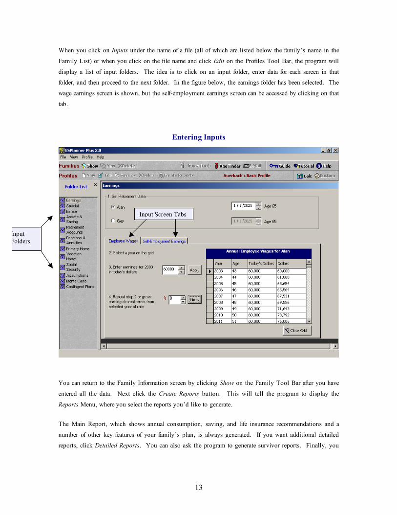
When you click on Inputs under the name of a file (all of which are listed below the family’s name in the
Family List) or when you click on the file name and click Edit on the Profiles Tool Bar, the program will
display a list of input folders. The idea is to click on an input folder, enter data for each screen in that
folder, and then proceed to the next folder. In the figure below, the earnings folder has been selected. The
wage earnings screen is shown, but the self-employment earnings screen can be accessed by clicking on that
tab.
Entering Inputs
You can return to the Family Information screen by clicking Show on the Family Tool Bar after you have
entered all the data. Next click the Create Reports button. This will tell the program to display the
Reports Menu, where you select the reports you’d like to generate.
The Main Report, which shows annual consumption, saving, and life insurance recommendations and a
number of other key features of your family’s plan, is always generated. If you want additional detailed
reports, click Detailed Reports. You can also ask the program to generate survivor reports. Finally, you
Input
Folders
Input Screen Tabs

14
can choose to generate Monte Carlo reports if you purchased ESPlannerPlus and previously activated
Monte Carlo on the Family Information screen.
The Monte Carlo results are based on 500 simulations. In each simulation, the program draws rates of
returns at random for regular assets as well as retirement account assets in each future year based on the
portfolio that users indicate will be held in that year. In the case of married or partnered households in
which each spouse/partner has retirement account assets, separate rates of return are drawn for each future
year for the couple’s regular assets and for each spouse’s/partner’s retirement account assets taking into
account the separate portfolios specified for regular assets and for each spouse’s/partner’s retirement account
assets.
As indicated below, there are a number of pre-programmed assets. But you can also enter your own assets.
All assets are assumed to be joint log normally distributed. The rates of return used to generate mean
returns and the variance/co-variance matrix of returns are based on data reported by Ibbotson and Morgan
Stanley. In all cases, we use the longest time series available.
In the cases of families who are married or partnered, ESPlanner generates survivor reports. These reports
show how survivors will fare if one of the two spouses/partners passes away, assuming the program’s
recommended amount of life insurance had been purchased and the couple had followed the program’s
recommended saving plan. The program generates these reports for every possible age at which each
spouse or partner may die. To see these survivor reports, you need to specify that ages at which you want
to assume the spouse and partner will die. The Report Menu screen also asks you to specify these ages
After you click Create Reports on the reports menu, the program will produce Excel files containing the
reports selected. The reports consist of charts and tabular displays of recommendations, balance sheets, etc.
You can use the Excel charting function to make additional charts and graphs. All of these reports can be
printed.
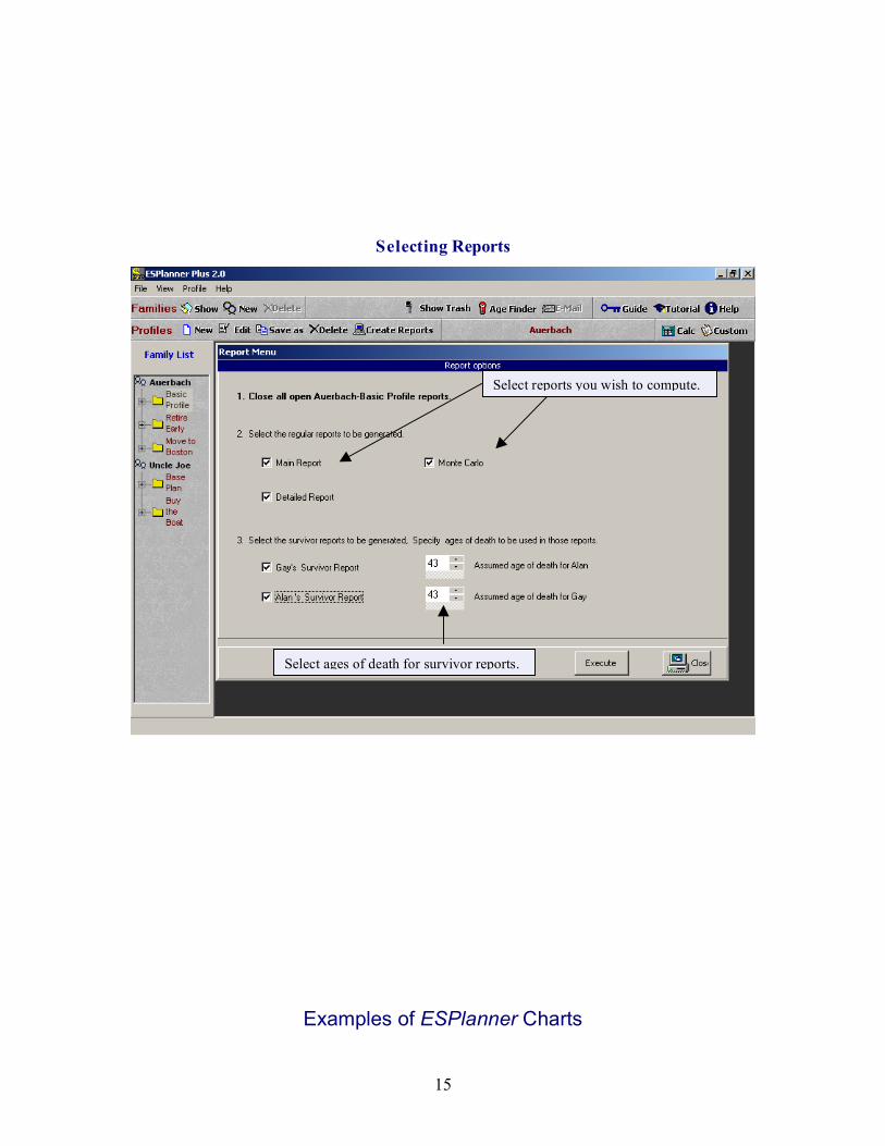
15
Selecting Reports
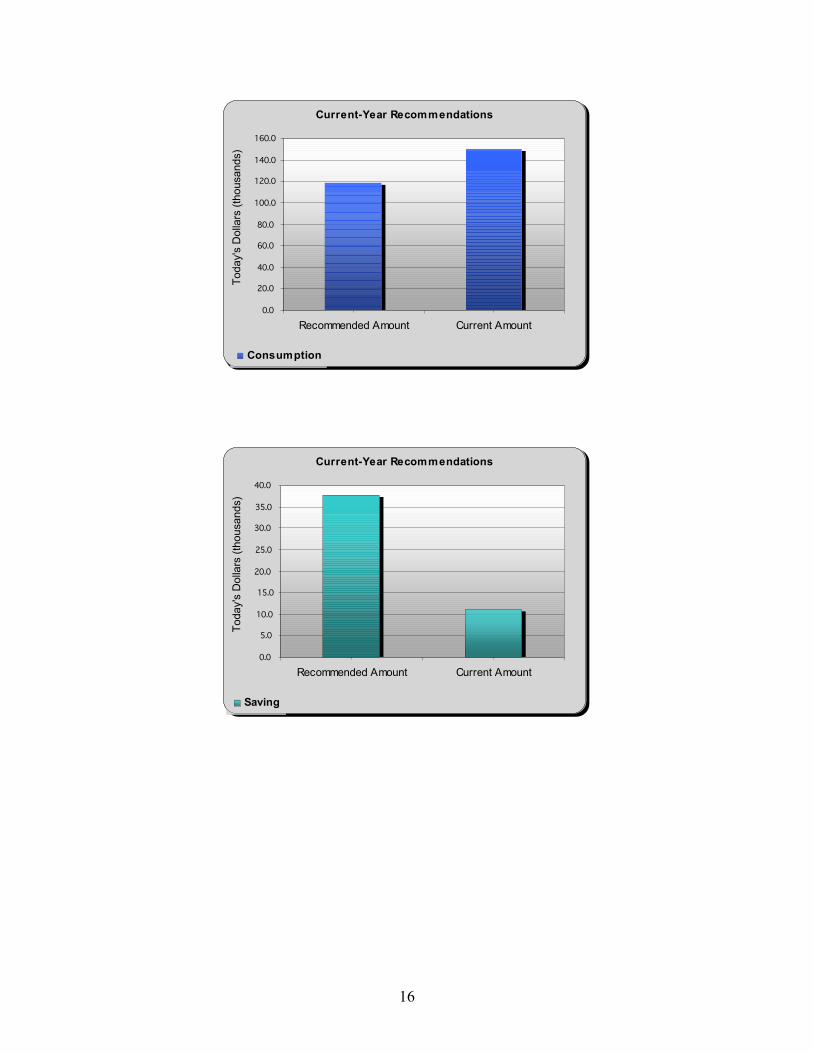
Examples of ESPlanner Charts
Select reports you wish to compute.
Select ages of death for survivor reports.
16
Current-Year Recommendations
0.0
20.0
40.0
60.0
80.0
100.0
120.0
140.0
160.0
Recommended Amount Current Amount
Today's
Dolla
rs (
thousands)
Consumption
Current-Year Recommendations
0.0
5.0
10.0
15.0
20.0
25.0
30.0
35.0
40.0
Recommended Amount Current Amount
Today's
Dolla
rs (
thousands)
Saving
17
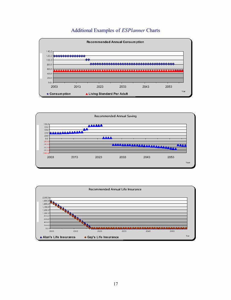
Additional Examples of ESPlanner Charts
18
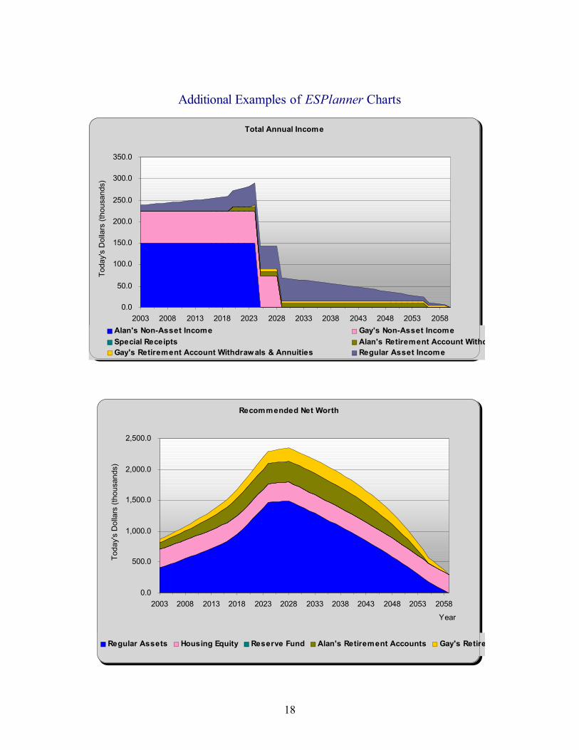
Additional Examples of ESPlanner Charts
Total Annual Income
0.0
50.0
100.0
150.0
200.0
250.0
300.0
350.0
2003 2008 2013 2018 2023 2028 2033 2038 2043 2048 2053 2058
Year
Today's
Dolla
rs (
thousands)
Alan's Non-Asset Income Gay's Non-Asset Income
Special Receipts Alan's Retirement Account Withdrawals & Annuities
Gay's Retirement Account Withdrawals & Annuities Regular Asset Income
Recommended Net Worth
0.0
500.0
1,000.0
1,500.0
2,000.0
2,500.0
2003 2008 2013 2018 2023 2028 2033 2038 2043 2048 2053 2058
Year
Today's
Dolla
rs (
thousands)
Regular Assets Housing Equity Reserve Fund Alan's Retirement Accounts Gay's Retirement Accounts
19
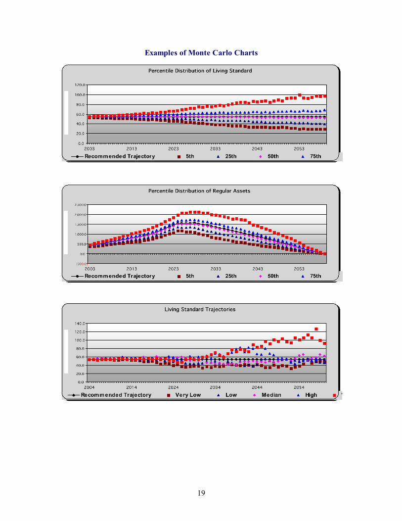
Examples of Monte Carlo Charts
20
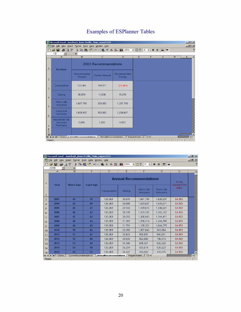
Examples of ESPlanner Tables

21
Additional Examples of ESPlanner Tables
22
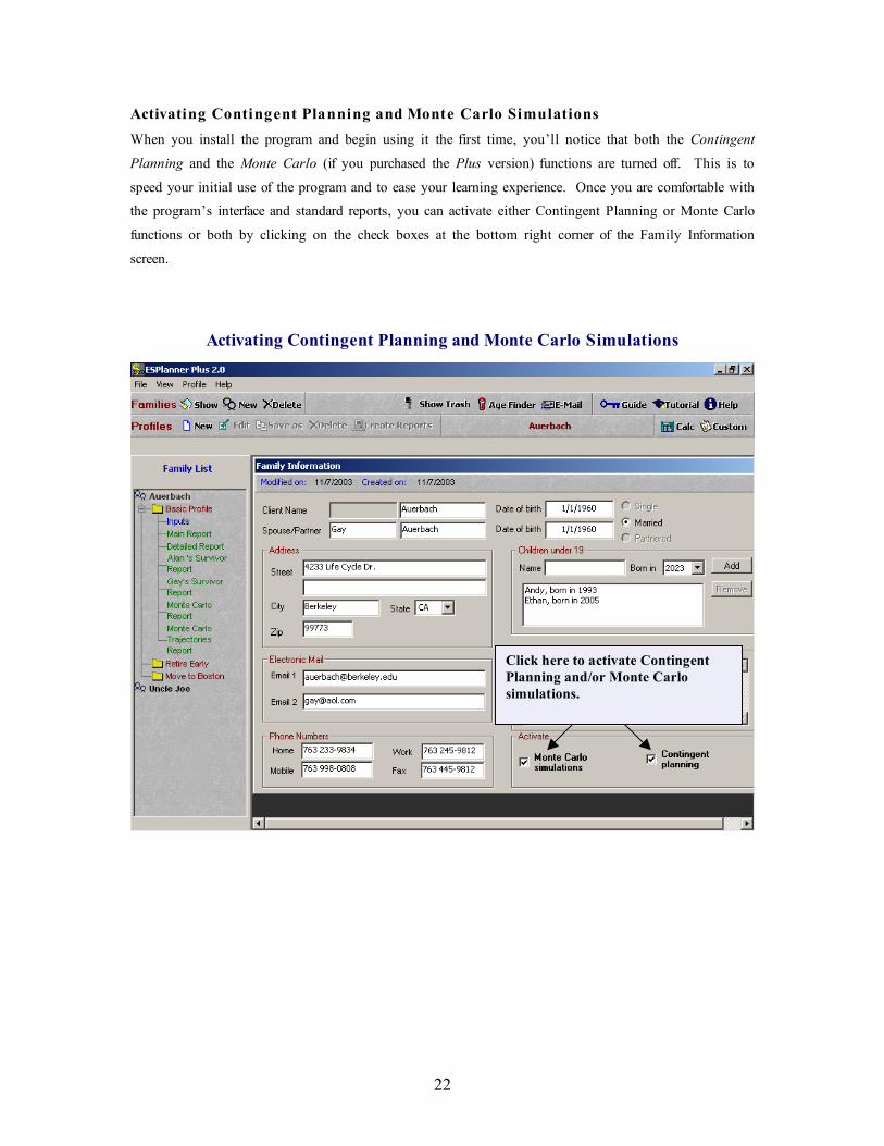
Activating Contingent Planning and Monte Carlo Simulations
When you install the program and begin using it the first time, you’ll notice that both the Contingent
Planning and the Monte Carlo (if you purchased the Plus version) functions are turned off. This is to
speed your initial use of the program and to ease your learning experience. Once you are comfortable with
the program’s interface and standard reports, you can activate either Contingent Planning or Monte Carlo
functions or both by clicking on the check boxes at the bottom right corner of the Family Information
screen.
Activating Contingent Planning and Monte Carlo Simulations
Click here to activate Contingent
Planning and/or Monte Carlo
simulations.

23
Optimizing Your Family’s Plans
Once you have generated a basic plan, there are a number of options you can explore to raise your family’s
sustainable living standards. Any changes that you make that do raise your family’s living standard will
show up in the program’s reports as higher recommended levels of consumption. Having your family retire
later, send its children to less expensive colleges, downsize their homes, move to states with lower income
taxes, and leave smaller bequests are examples of ways in which to raise your family’s consumption levels.
The great advantage of ESPlanner is being able to learn, within seconds, how these choices would affect
your family’s living standard (measured in terms of recommended consumption) knowing that all the tax
and social security benefit implications of those choices are being fully considered.
Households that cannot perfectly smooth their living standards over their lifetimes, because doing so would
require going into debt, are forced to live at a lower living standard when young than when old. For such
households, one needs to consider how each particular input change affects not just consumption when
young, but also when old.
In addition to helping your family to sort out choices like those just mentioned ESPlanner can be used to
make sure your family’s plan minimizes lifetime tax payments and maximizes lifetime social security
benefits. When it comes to reducing lifetime tax payments, there are several options to consider. One
thing to check is whether your family should contribute more or less to tax-deferred accounts. Although it
is commonly believed that maximizing contributions to tax-deferred accounts, including 401(k) and
traditional IRA plans, lowers lifetime tax payments, this is not necessarily the case for three reasons. First,
withdrawals of principal plus interest from tax-deferred accounts can put your family into higher tax
brackets. Second, these withdrawals can trigger federal income taxation of your family’s social security
benefits. And third, tax rates may be higher when your family makes its withdrawals. Note, in this regard,
that the Assumptions folder allows you to specify future increases in federal income tax rates, state income
tax rates, or payroll tax rates.
Another option to consider is the timing of when you and your spouse/partner begin to make withdrawals
from your tax-deferred accounts. The program allows you to choose the age of retirement account
withdrawals. The longer one delays withdrawing benefits from tax-deferred retirement accounts, the greater
the savings from being able to earn capital income on a tax-free basis. However, taking out smaller
amounts over longer periods of time can affect the extend of social security benefit taxation as well as the
income tax rates at which withdrawals are taxed.
A third option to explore is the timing of when your family begins to collect its social security benefits.
Different initial dates of collection will affect not just the duration of benefit receipt, but also the amount of
the benefits collected each year. The initial collection date can also affect the degree to which these benefits
are subject to taxation under federal and state income taxes. For example, having a family member start
receiving social security benefits at age 65 as well as initiating 401(k) withdrawals at age 65 may increase

24
lifetime tax payments relative to having the family member receive social security benefits starting at age 62
and wait until age 71 to begin withdrawing retirement account assets.
A fourth issue to explore is the order in which to withdraw funds from retirement accounts. One can, for
example, tell the program to withdrawal funds first from 401(k) plans, next from traditional IRAs, and
finally from Roth IRAs. But this may not minimize lifetime tax payments.
When it comes to decisions about when and how to make retirement account withdrawals and when to start
collecting social security benefits, there are no general rules that minimize lifetime tax payments and
maximize lifetime social security benefits. The best decision for a particular household depends on that
household’s other economic variables and life-style decisions. But ESPlanner’s main and detailed reports
run within seconds on reasonably fast computers, so you can very quickly explore alternative strategies and
find the best combination for your family.
Monte Carlo Simulations
ESPlannerPlus’ Monte Carlo simulations are designed to let you see how alternative portfolio choices will
affect both the level and variability of your family’s living standard, income levels, and regular and
retirement account asset levels through time. Unlike other Monte Carlo simulators that only show the
variability of a household’s assets at retirement, ESPlanner recognizes that you will not wait until
retirement to adjust its consumption to the returns it earns on its savings. The program uses dynamic
programming to determine how your family would adjust its consumption spending level each year given
the realized rates of return and a desire for a smooth living standard going forward.
The dynamic program also takes into account the fact that receiving higher or lower rates of return in a
given year will affect one’s tax liabilities in the current as well as all future years. Stated differently, our
Monte Carlo simulations take full account of the tax implications of the path of returns that your family
may earn on both its regular assets and retirement accounts.
The actual Monte Carlo simulations are the result of considering 500 paths of randomly drawn rates of
return earned on both regular and retirement account assets. If, for example, your family is married, the
program will draw rates of return for each year for regular assets as well as for each spouse’s retirement
accounts taking into account the composition of regular assets and of each spouse’s retirement account
assets in the particular year in question.
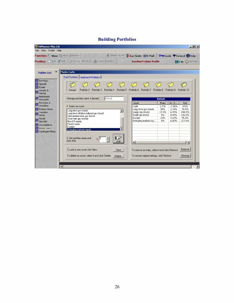
To be more precise, the program includes 12 “canned securities,” such as large cap stock, corporate bonds,
and European equities, which you can use to build up to 10 different portfolios for your family. The
program takes into account how these 12 securities have performed and co-varied historically.

25
You can also add additional securities that you want to include in the 10 portfolios. In entering your own
assets, the program asks you about their expected rates of return and variability relative to large cap stock.
The program assumes that the returns on your own assets do not co-vary with the 12 canned securities.
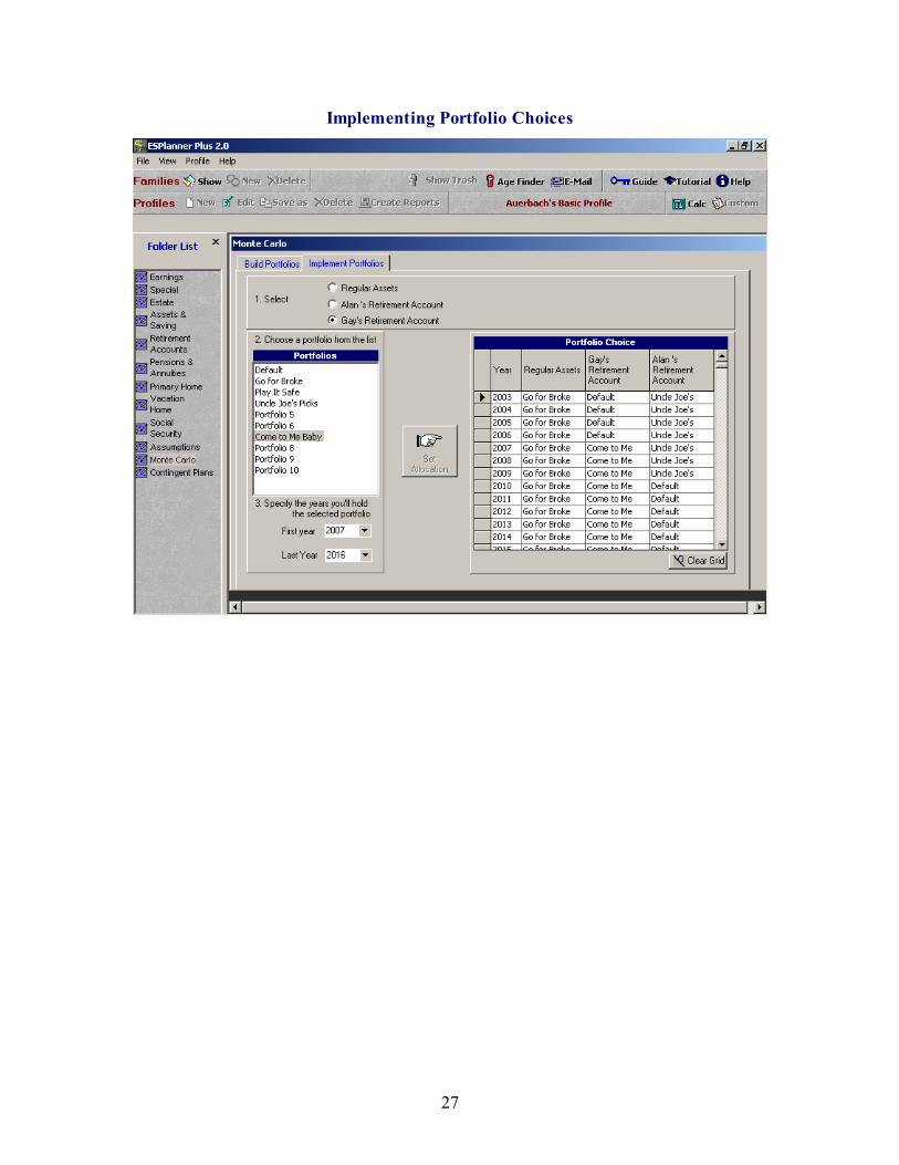
Once you’ve built (specified) your portfolios, you can tell the program which of these portfolios the family
will hold in each future year when it comes to his/her regular assets, which of these portfolios the family
will hold in each future year when it comes to his/her retirement account assets, and which of these
portfolios the family’s spouse/partner will hold in each future year when it comes to the spouse’s/partner’s
retirement account assets. The following screens indicate how you can build and implement portfolios.
In each of the 500 the Monte Carlo simulations the program draws rates of return at random and for each
future year for each of the 12 canned securities as well as the individualize securities you’ve entered. These
annual draws take into account the covariance (the co-movement) of the returns on these securities as well
as their expected returns. The program then uses these rates of return to determine how the particular
portfolios being held by the family in its regular assets and retirement accounts will fare. As the simulation
moves forward from one year to the next, the program adjusts consumption and saving levels as dictated by
the dynamic program, which is run prior to generating the simulations. Again, the dynamic program takes
into account all possible return outcomes as well as their tax implications in determining how the
household can expect to smooth its living standard going forward.
Borrowing Constraints
Many, if not most, young and middle-aged households are borrowing or credit constrained. Such
households typically have large “off-the-top” expenses, including mortgage payments, loan payments,
childcare, and college tuition. They also either can’t or don’t want to borrow against their future income.
For these households, perfectly smoothing their members’ living standards through time is infeasible
because it requires going into debt.
26
Building Portfolios
27
Implementing Portfolio Choices

28
ESPlanner takes borrowing limits into account in its calculations and recommendations. Specifically, it
smoothes each household’s living standard to the maximum extent possible without violating the
household’s self-declared non-mortgage borrowing limit. The software permits multiple intervals (time
periods) during which the household is borrowing constrained. It not only minimizes difference in living
standards across such intervals, it also smoothes living standards within each interval.
You can readily tell when borrowing limitations prevent your family from achieving a perfectly smooth
living standard. All you need to do is to examine the regular asset report. If regular assets equal the
borrowing limit (set at zero in most cases), you know that the household is borrowing constrained prior to
and including the year that regular assets hit the limit. In the first subsequent year that regular assets rise
about the limit, you’ll see recommended consumption increasing as well. The reason is that the
household is no longer constrained and can consume at a higher level.
To make this more concrete, consider the case of a low-income couple that will receive a $2 million
distribution from a trust in ten years. Assume the couple can’t borrow against the future income.
ESPlanner will recommend the couple spend down its assets so they reach zero in the year before the $2
million is received. In the year it’s received, asset will go from zero to a large positive amount and
recommended consumption will rise. We illustrate this below in Joe and Sally Receive an Inheritance.
29
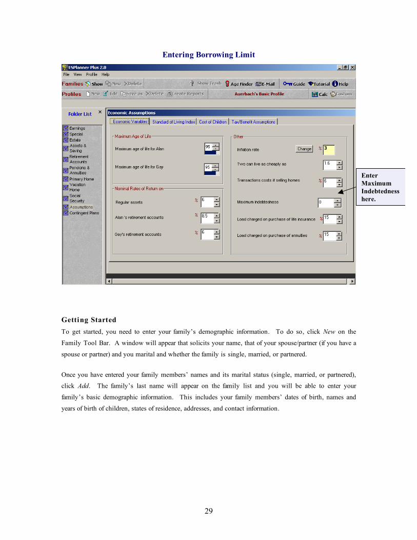
Entering Borrowing Limit
Getting Started
To get started, you need to enter your family’s demographic information. To do so, click New on the
Family Tool Bar. A window will appear that solicits your name, that of your spouse/partner (if you have a
spouse or partner) and you marital and whether the family is single, married, or partnered.
Once you have entered your family members’ names and its marital status (single, married, or partnered),
click Add. The family’s last name will appear on the family list and you will be able to enter your
family’s basic demographic information. This includes your family members’ dates of birth, names and
years of birth of children, states of residence, addresses, and contact information.
Enter
Maximum
Indebtedness
here.
30
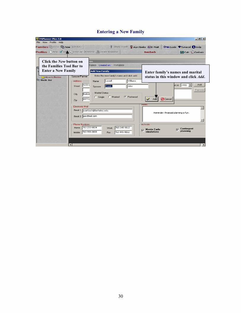
Entering a New Family
Click the New button on
the Families Tool Bar to
Enter a New Family
Enter family’s names and marital
status in this window and click Add.

31
Entering Basic Information for a New Family
Enter names,
dates of birth,
addresses,
names and
birth years of
children,
contact
information,
and any special
notes.
32
Joe and Sal ly
To help you learn how to use ESPlanner’s interface and interpret its results, we start out with a simple
case and then modify inputs to illustrate ESPlanner’s versatility in handling multiple financial
circumstances and objectives. This case was run without activating contingent planning or Monte Carlo
simulations, which we illustrate in subsequent cases. Because contingent planning is turned off, the values
of contingent variables, like the wife’s earnings if the husband passes away, are assumed to be the same as
the non-contingent variables (the wife’s earnings if the husband doesn’t pass away prior to reaching his
maximum age of life). And because the Monte Carlo simulations are turned off, we enter the rates of return
on regular and retirement account assets in the Assumptions input folder.
Note that if you set up and run the cases presented here, your results may differ from those presented
because we are continuously updating tax and Social Security benefit formulae. Also, this tutorial was
written in 2003, and it may be a later year as you read this.
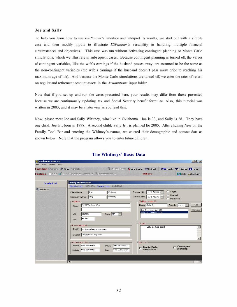
Now, please meet Joe and Sally Whitney, who live in Oklahoma. Joe is 33, and Sally is 28. They have
one child, Joe Jr., born in 1998. A second child, Sally Jr., is planned for 2005. After clicking New on the
Family Tool Bar and entering the Whitney’s names, we entered their demographic and contact data as
shown below. Note that the program allows you to enter future children.
The Whitneys’ Basic Data
33
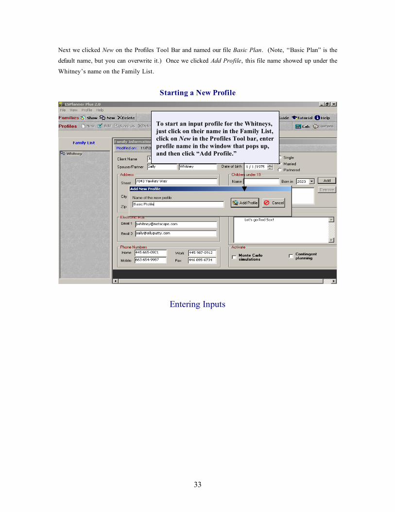
Next we clicked New on the Profiles Tool Bar and named our file Basic Plan. (Note, “Basic Plan” is the
default name, but you can overwrite it.) Once we clicked Add Profile, this file name showed up under the
Whitney’s name on the Family List.
Starting a New Profile
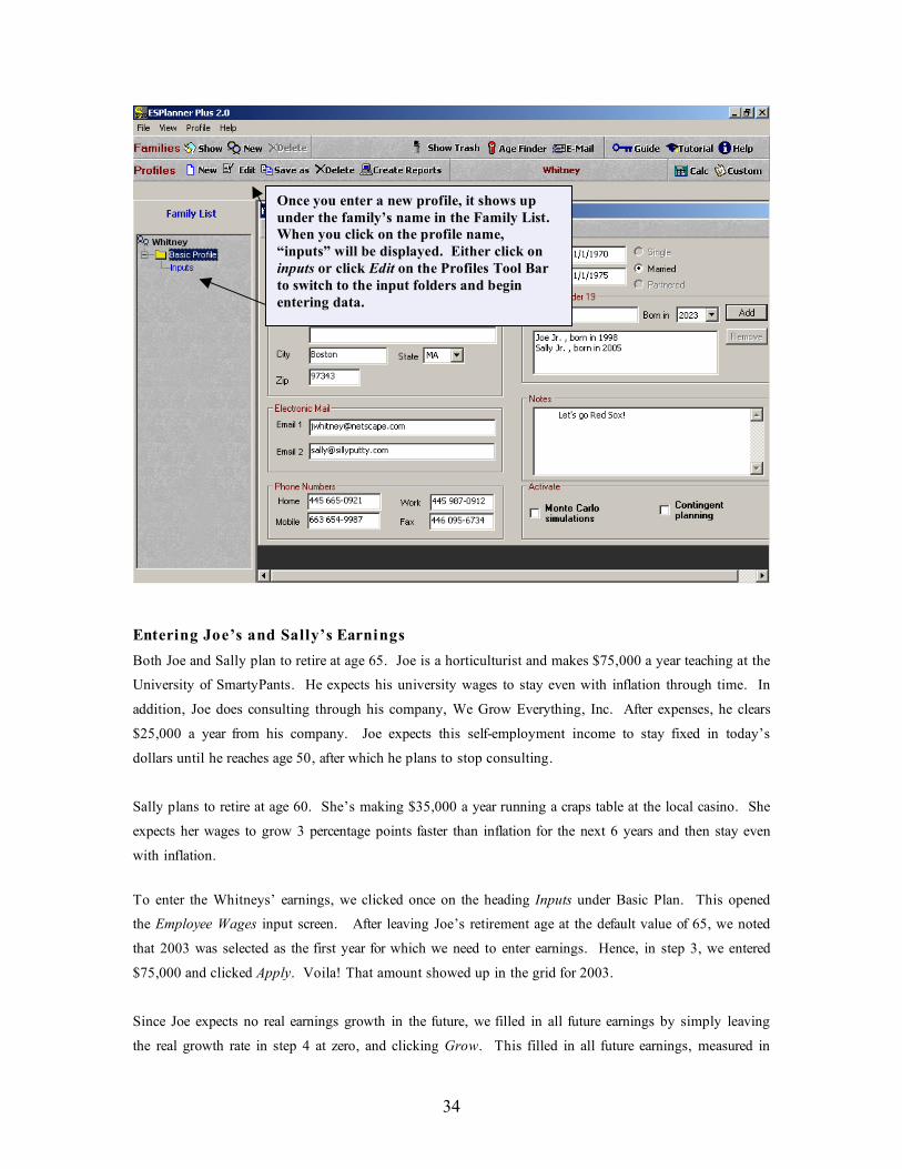
Entering Inputs
To start an input profile for the Whitneys,
just click on their name in the Family List,
click on New in the Profiles Tool bar, enter
profile name in the window that pops up,
and then click “Add Profile.”
34
Entering Joe’s and Sally’s Earnings
Both Joe and Sally plan to retire at age 65. Joe is a horticulturist and makes $75,000 a year teaching at the
University of SmartyPants. He expects his university wages to stay even with inflation through time. In
addition, Joe does consulting through his company, We Grow Everything, Inc. After expenses, he clears
$25,000 a year from his company. Joe expects this self-employment income to stay fixed in today’s
dollars until he reaches age 50, after which he plans to stop consulting.
Sally plans to retire at age 60. She’s making $35,000 a year running a craps table at the local casino. She
expects her wages to grow 3 percentage points faster than inflation for the next 6 years and then stay even
with inflation.
To enter the Whitneys’ earnings, we clicked once on the heading Inputs under Basic Plan. This opened
the Employee Wages input screen. After leaving Joe’s retirement age at the default value of 65, we noted
that 2003 was selected as the first year for which we need to enter earnings. Hence, in step 3, we entered
$75,000 and clicked Apply. Voila! That amount showed up in the grid for 2003.
Since Joe expects no real earnings growth in the future, we filled in all future earnings by simply leaving
the real growth rate in step 4 at zero, and clicking Grow. This filled in all future earnings, measured in
Once you enter a new profile, it shows up
under the family’s name in the Family List.
When you click on the profile name,
“inputs” will be displayed. Either click on
inputs or click Edit on the Profiles Tool Bar
to switch to the input folders and begin
entering data.

35
today’s dollars, as $75,000. The grid also displays the actual dollar amounts of future earnings in the
column under the heading Dollars. The conversion of earnings measured into today’s dollars into earnings
in actual dollars is based on the assumed inflation rate, which is set in the Assumptions input folder. The
default value for the annual inflation rate is 3 percent.
Next we entered Joe’s self-employment earnings by clicking on the – yes, you got it – Self-Employment
Earnings tab. We selected 2003 and entered $25,000. Then we grew those earnings at a zero percent
growth rate. Finally, we selected 2020, the year Joe becomes 50, entered earnings of zero for that year, and
then hit the Grow button. This zeroed out Joe’s self-employment earnings from age 51 through 65.
To enter Sally’s earnings, we simply selected Sally’s name in step 1. Next we set her retirement age to
60. But after entering her 2003 earnings at $35,000, we set the real growth rate in step 3 at 3 percent and
clicked Grow. This grew Sally’s earnings, measured in today’s dollars, by 3 percent through age 64 – her
last year of work. But Sally’s earnings are going to grow for only 6 years, so we next selected year 2009
in the grid, set the growth rate to zero, and clicked Grow. This generated the earnings inputs shown
below.
Entering Joe’s Employee Wages
To enter Joe’s earnings, measured in today’s
dollars, we entered $75,000 for 2003 in step 3,
and grew his earnings at a zero rate in step 4.

36
Entering Joe’s Self-Employment Earnings
To enter Joe’s
consulting
income, we
selected the self-
employment
earnings tab.
Then we entered
$25,000 for 2003,
grew this amount
at a zero rate,
selected 2020,
entered zero, and
clicked Grow.

37
Entering Sally’s Earnings
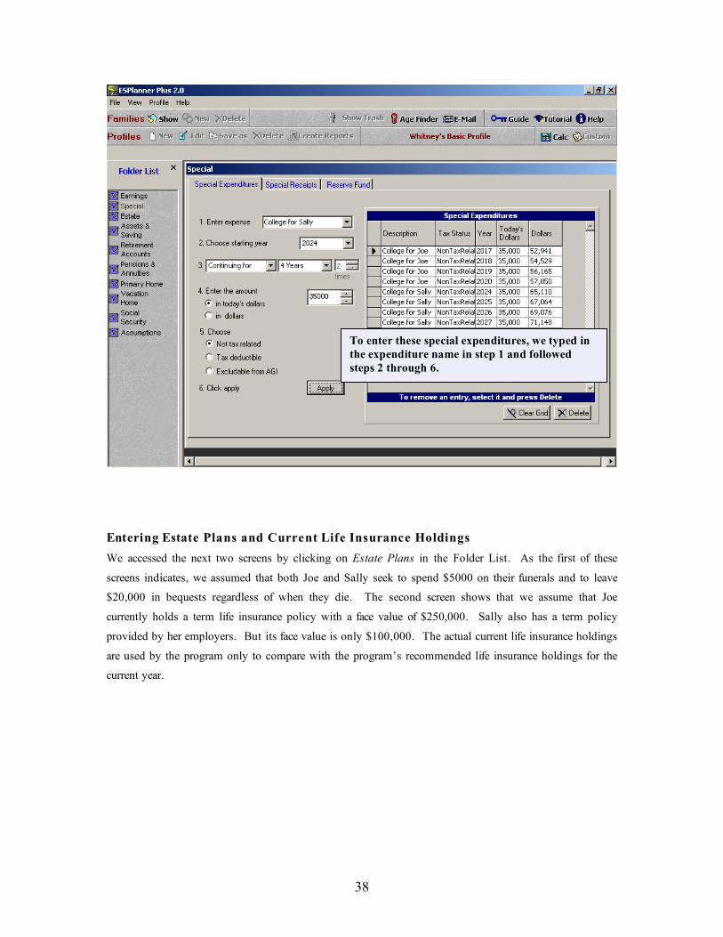
Entering the Whitneys’ Special Expenses
Joe and Sally want to send both of their children to their alma mater, NotforDummies U. The cost in 2003
of a NDU education was $35,000, and worth every penny. Joe and Sally expect to pay that amount in
today’s dollars when their children reach age 19, which occurs in 2017 for Joe Jr. and 2024 for Sally Jr.
To enter these special expenses, we clicked Special on the Folder List. The program opened the Special
Expenditures screen. We then typed in College for Joe Jr. in the field in step 1, selected 2017 for step 2,
indicated in step 3 that the expense would continue for 4 years, specified in step 4 that the expense was in
today’s dollars, entered the amount, specified in step 5 that the expense was Not Tax-Related, and then
clicked Apply. We then repeated these steps for Sally Junior's college tuition, except we specified that the
expense would begin in 2024. The next screen shot shows the Special Expenditures screen after these
inputs have been entered.
Entering College Tuition for Joe Jr. and Sally Jr.
To enter Sally’s earnings, measured in today’s
dollars, we set her retirement age to 69 and
entered $35,000 for 2003. Next we set the growth
rate to 3%, clicked Grow, then selected 2009, set
the growth rate to zero and clicked Grow.
38
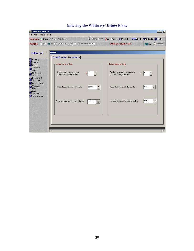
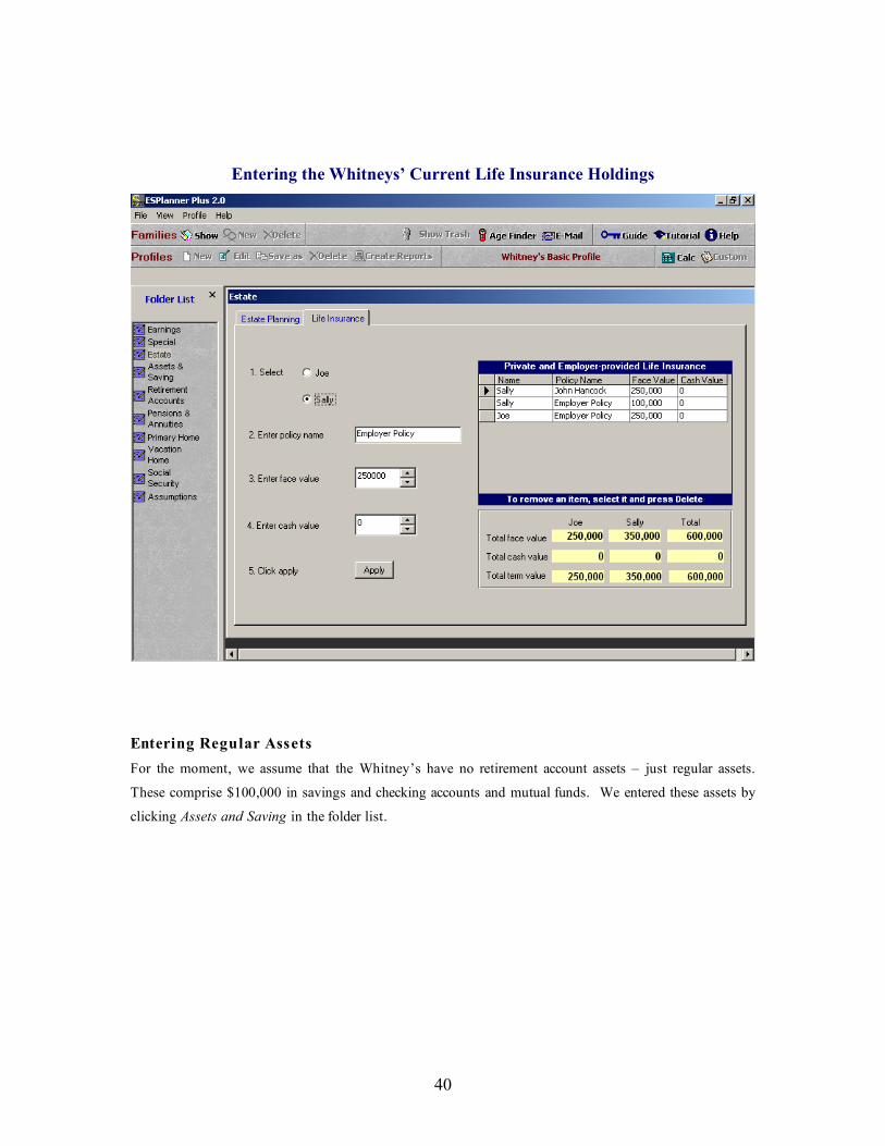
Entering Estate Plans and Current Life Insurance Holdings
We accessed the next two screens by clicking on Estate Plans in the Folder List. As the first of these
screens indicates, we assumed that both Joe and Sally seek to spend $5000 on their funerals and to leave
$20,000 in bequests regardless of when they die. The second screen shows that we assume that Joe
currently holds a term life insurance policy with a face value of $250,000. Sally also has a term policy
provided by her employers. But its face value is only $100,000. The actual current life insurance holdings
are used by the program only to compare with the program’s recommended life insurance holdings for the
current year.
To enter these special expenditures, we typed in
the expenditure name in step 1 and followed
steps 2 through 6.
39
Entering the Whitneys’ Estate Plans
40
Entering the Whitneys’ Current Life Insurance Holdings
Entering Regular Assets
For the moment, we assume that the Whitney’s have no retirement account assets – just regular assets.
These comprise $100,000 in savings and checking accounts and mutual funds. We entered these assets by
clicking Assets and Saving in the folder list.
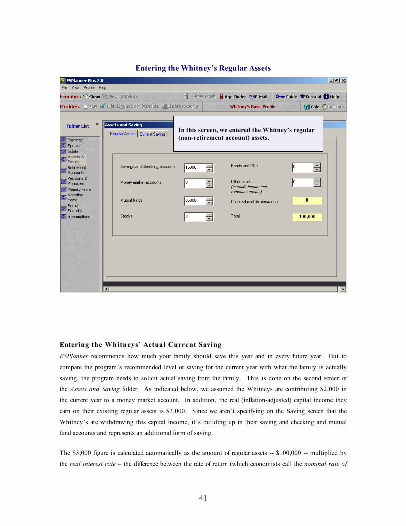
41
Entering the Whitney’s Regular Assets
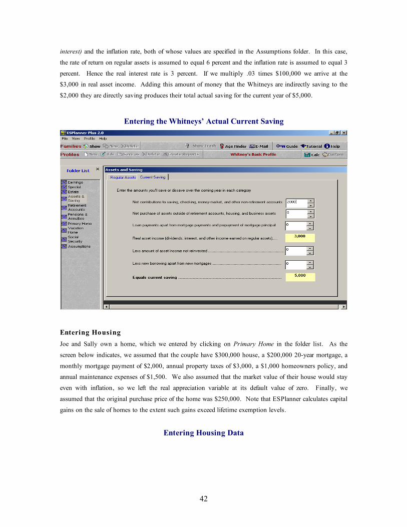
Entering the Whitneys’ Actual Current Saving
ESPlanner recommends how much your family should save this year and in every future year. But to
compare the program’s recommended level of saving for the current year with what the family is actually
saving, the program needs to solicit actual saving from the family. This is done on the second screen of
the Assets and Saving folder. As indicated below, we assumed the Whitneys are contributing $2,000 in
the current year to a money market account. In addition, the real (inflation-adjusted) capital income they
earn on their existing regular assets is $3,000. Since we aren’t specifying on the Saving screen that the
Whitney’s are withdrawing this capital income, it’s building up in their saving and checking and mutual
fund accounts and represents an additional form of saving.
The $3,000 figure is calculated automatically as the amount of regular assets -- $100,000 -- multiplied by
the real interest rate – the difference between the rate of return (which economists call the nominal rate of
In this screen, we entered the Whitney’s regular
(non-retirement account) assets.
42
interest) and the inflation rate, both of whose values are specified in the Assumptions folder. In this case,
the rate of return on regular assets is assumed to equal 6 percent and the inflation rate is assumed to equal 3
percent. Hence the real interest rate is 3 percent. If we multiply .03 times $100,000 we arrive at the
$3,000 in real asset income. Adding this amount of money that the Whitneys are indirectly saving to the
$2,000 they are directly saving produces their total actual saving for the current year of $5,000.
Entering the Whitneys’ Actual Current Saving
Entering Housing
Joe and Sally own a home, which we entered by clicking on Primary Home in the folder list. As the
screen below indicates, we assumed that the couple have $300,000 house, a $200,000 20-year mortgage, a
monthly mortgage payment of $2,000, annual property taxes of $3,000, a $1,000 homeowners policy, and
annual maintenance expenses of $1,500. We also assumed that the market value of their house would stay
even with inflation, so we left the real appreciation variable at its default value of zero. Finally, we
assumed that the original purchase price of the home was $250,000. Note that ESPlanner calculates capital
gains on the sale of homes to the extent such gains exceed lifetime exemption levels.
Entering Housing Data

43
Entering Social Security Benefit Collection Dates and Covered Earnings
We have two more input folders to complete prior to computing our first case. The first is Social Security
benefits, which we access by clicking the Social Security folder. This folder has three screens. The first
solicits future Social Security benefit collection dates for those not collecting and for those already
collecting benefits, it solicits the monthly benefit amount and the date benefits were first received. (We
need this info to correctly calculate spousal survivor benefits.) As indicated below, we assume that both
Joe and Sally begin receiving their Social Security benefits at age 65.
Entering inputs on the housing screens
is easy. There is one trick, however.
You need to set the value of the home to
zero to switch to renting and set
monthly rent to zero to switch to
owning.

44
Entering Joe’s and Sally’s Social Security Benefit Collection Dates
The next Social Security input screen asks about future Social Security-covered earnings. Since both Joe
and Sally are in covered employment, we clicked the Copy button to copy their wage earnings into the
relevant grids. Since self-employment earnings are automatically covered by Social Security, the program
already knows to include Joe’s self-employment earnings in assessing FICA taxes and determining Social
Security covered earnings for purposes of determining Social Security benefits.
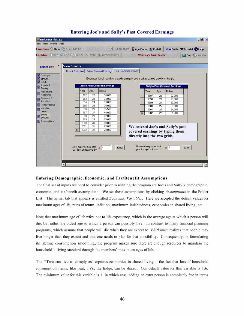
The last Social Security screen solicits past covered earnings, whether from employee wages or self-
employment earnings. Here we simply entered values for both Joe and Sue.

45
Entering Joe’s and Sally’s Future Covered Earnings
Since Joe’s and Sally’s wage
earnings are covered by Social
Security, we entered their future
covered wages simply by clicking
Copy.
46
Entering Joe’s and Sally’s Past Covered Earnings
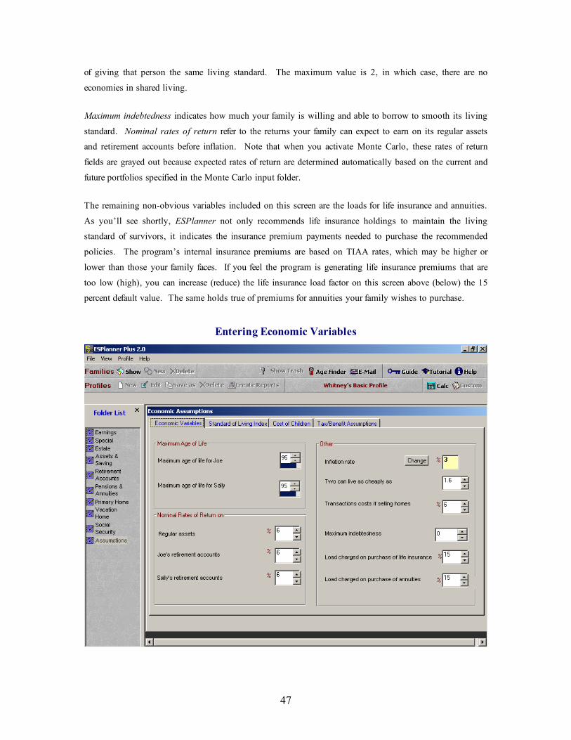
Entering Demographic, Economic, and Tax/Benefit Assumptions
The final set of inputs we need to consider prior to running the program are Joe’s and Sally’s demographic,
economic, and tax/benefit assumptions. We set these assumptions by clicking Assumptions in the Folder
List. The initial tab that appears is entitled Economic Variables. Here we accepted the default values for
maximum ages of life, rates of return, inflation, maximum indebtedness, economies in shared living, etc.
Note that maximum age of life refers not to life expectancy, which is the average age at which a person will
die, but rather the oldest age to which a person can possibly live. In contrast to many financial planning
programs, which assume that people will die when they are expect to, ESPlanner realizes that people may
live longer than they expect and that one needs to plan for that possibility. Consequently, in formulating
its lifetime consumption smoothing, the program makes sure there are enough resources to maintain the
household’s living standard through the members’ maximum ages of life.
The “Two can live as cheaply as” captures economies in shared living – the fact that lots of household
consumption items, like heat, TVs, the fridge, can be shared. Our default value for this variable is 1.6.
The minimum value for this variable is 1, in which case, adding an extra person is completely free in terms
We entered Joe’s and Sally’s past
covered earnings by typing them
directly into the two grids.
47
of giving that person the same living standard. The maximum value is 2, in which case, there are no
economies in shared living.
Maximum indebtedness indicates how much your family is willing and able to borrow to smooth its living
standard. Nominal rates of return refer to the returns your family can expect to earn on its regular assets
and retirement accounts before inflation. Note that when you activate Monte Carlo, these rates of return
fields are grayed out because expected rates of return are determined automatically based on the current and
future portfolios specified in the Monte Carlo input folder.
The remaining non-obvious variables included on this screen are the loads for life insurance and annuities.
As you’ll see shortly, ESPlanner not only recommends life insurance holdings to maintain the living
standard of survivors, it indicates the insurance premium payments needed to purchase the recommended
policies. The program’s internal insurance premiums are based on TIAA rates, which may be higher or
lower than those your family faces. If you feel the program is generating life insurance premiums that are
too low (high), you can increase (reduce) the life insurance load factor on this screen above (below) the 15
percent default value. The same holds true of premiums for annuities your family wishes to purchase.
Entering Economic Variables

48
The next Assumptions input screen is called Standard of Living Index. This screen allows you to override
the program’s default assumption, namely that your family wants to have the same living standard each
period. This default assumption is imposed by initially setting all values of the standard of living index to
100. The value of the index for the current year, in this case 2030, is set at 100 and can’t be changed. By
altering values of the index in years after the current year, you can tell the program how you want your
family’s living standard to change in future years relative to the current year.
In Joe’s and Sally’s case, we assumed the couple wishes to have a 10 percent higher living standard when
Joe hits age 70 and Sally reaches age 65, which occurs in 2040. To tell the program this, we selected
2040, enter 110 in step 2, clicked apply, and then grew 110 at a growth rate of zero. This filled in values
of 110 from 2040 onward and told the program to make the living standard 10 percent higher in each year
after Sally retires than it was before she retires.
Entering the Whitneys’ Preferences about Changes in their Living Standard
Note that the program automatically adjusts its consumption recommendations to take into account how
many mouths there are to feed in a given year in the household, the fact that two can live more cheaply than
To make the Whitneys’ living standard 10 percent
higher after 2039, we selected 2040, entered 110,
and then grew 110 at a zero growth rate.
49
one, and that children are not necessarily as expensive as adults with respect to generating a given living
standard. Hence, don’t use the standard of living index to try to adjust recommended consumption for
changes over time in the household’s composition. The program does that on its own by assuming that
children leave the household at age 19, leaving fewer child mouths to feed, and that when a spouse or
partner dies, there is one fewer adult mouth to feed.
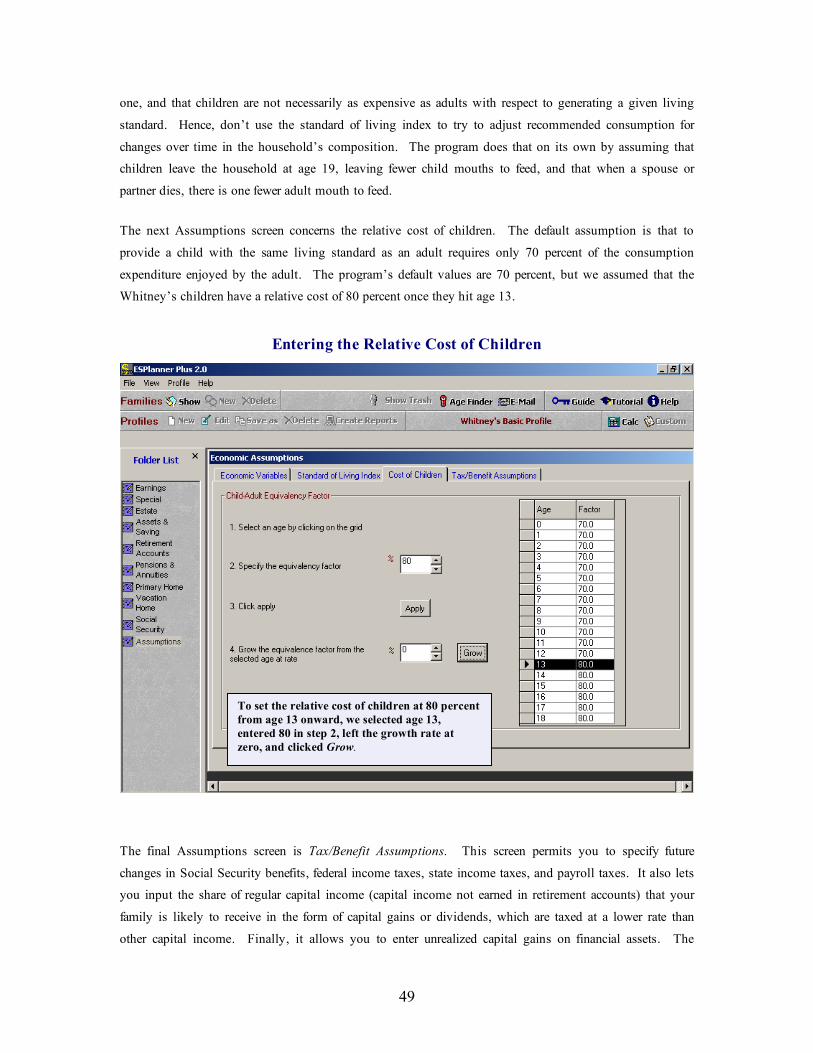
The next Assumptions screen concerns the relative cost of children. The default assumption is that to
provide a child with the same living standard as an adult requires only 70 percent of the consumption
expenditure enjoyed by the adult. The program’s default values are 70 percent, but we assumed that the
Whitney’s children have a relative cost of 80 percent once they hit age 13.
Entering the Relative Cost of Children
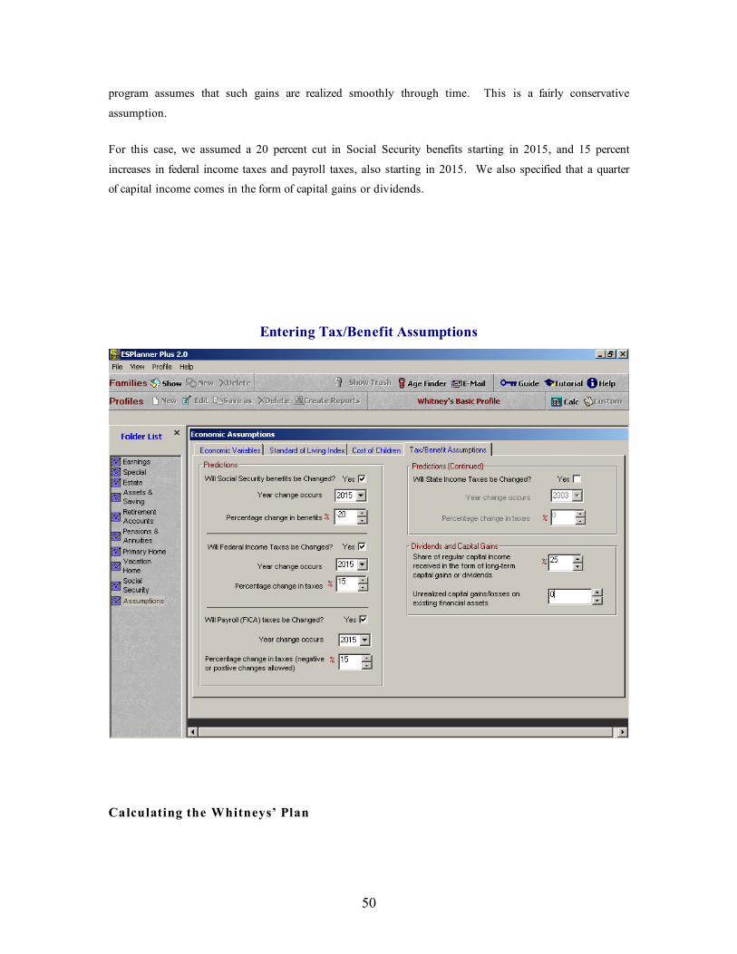
The final Assumptions screen is Tax/Benefit Assumptions. This screen permits you to specify future
changes in Social Security benefits, federal income taxes, state income taxes, and payroll taxes. It also lets
you input the share of regular capital income (capital income not earned in retirement accounts) that your
family is likely to receive in the form of capital gains or dividends, which are taxed at a lower rate than
other capital income. Finally, it allows you to enter unrealized capital gains on financial assets. The
To set the relative cost of children at 80 percent
from age 13 onward, we selected age 13,
entered 80 in step 2, left the growth rate at
zero, and clicked Grow.
50
program assumes that such gains are realized smoothly through time. This is a fairly conservative
assumption.
For this case, we assumed a 20 percent cut in Social Security benefits starting in 2015, and 15 percent
increases in federal income taxes and payroll taxes, also starting in 2015. We also specified that a quarter
of capital income comes in the form of capital gains or dividends.
Entering Tax/Benefit Assumptions
Calculating the Whitneys’ Plan
51
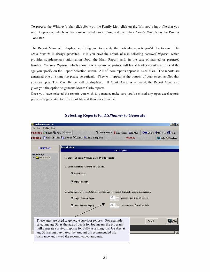
To process the Whitney’s plan click Show on the Family List, click on the Whitney’s input file that you
wish to process, which in this case is called Basic Plan, and then click Create Reports on the Profiles
Tool Bar.
The Report Menu will display permitting you to specify the particular reports you’d like to run. The
Main Reports is always generated. But you have the option of also selecting Detailed Reports, which
provides supplementary information about the Main Report, and, in the case of married or partnered
families, Survivor Reports, which show how a spouse or partner will fare if his/her counterpart dies at the
age you specify on the Report Selection screen. All of these reports appear in Excel files. The reports are
generated one at a time (so please be patient). They will appear at the bottom of your screen as files that
you can open. The Main Report will be displayed. If Monte Carlo is activated, the Report Menu also
gives you the option to generate Monte Carlo reports.
Once you have selected the reports you wish to generate, make sure you’ve closed any open excel reports
previously generated for this input file and then click Execute.
Selecting Reports for ESPlanner to Generate
These ages are used to generate survivor reports. For example,
selecting age 33 as the age of death for Joe means the program
will generate survivor reports for Sally assuming that Joe dies at
age 33 having purchased the amount of recommended life
insurance and saved the recommended amounts.

52
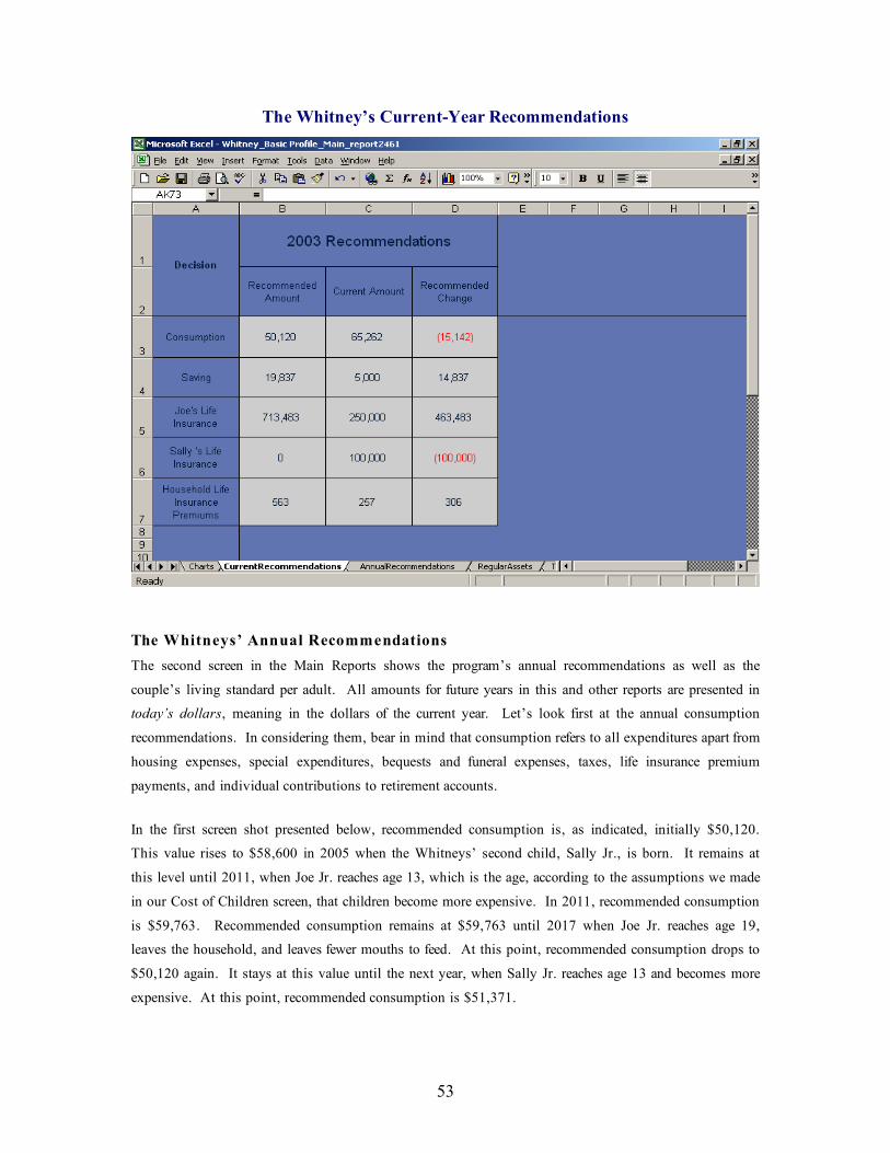
The Whitney’s Current-Year Recommendations
The first worksheet you’ll see in the Main Reports provides a set of charts that summarize the program’s
recommendations. Subsequent worksheets present the results in tabular form. The Current
Recommendations report, copied below, is an example. It shows how much the Whitney’s should save,
consume, and insure in the current year. As indicated in the screen shot presented below, the Whitneys are
consuming too much. The program recommends they spend $50,120 on consumption and save $19,837
in the current year. Given the couple’s actual current consumption and saving, the program recommends
they reduce their consumption expenditures by $15,142 and spend $306 more on life insurance premiums.
The net recommended reduction in expenditures is thus $14,837, which, up to a dollar, is the program’s
recommended increase in saving.
How does the program determine that the amount the Whitneys are currently consuming is $65,262? It
does so by starting with the Whitneys’ total current income and subtracting all its non-consumption
expenditures, including its actual current saving. To be precise, the program subtracts from total current
income the sum of actual saving, any current special expenditures, current contributions to the reserve fund,
current housing expenditures, current actual life insurance premium payments, current non-employer
contributions to retirement accounts, and current taxes.
The program also indicates that Joe’s life is underinsured to the tune of $484,264 and that Sally’s life is
over insured by $100,000. The additional life insurance on Joe’s life is needed, in the event Joe dies in the
current year, to maintain Sally’s living standard and that of the children at the same level through time as
they would otherwise have enjoyed. The program recommends no life insurance on Sally’s life because
were Sally to die with no life insurance, Joe and the children would enjoy a higher living standard than
would otherwise be the case.
53
The Whitney’s Current-Year Recommendations
The Whitneys’ Annual Recommendations
The second screen in the Main Reports shows the program’s annual recommendations as well as the
couple’s living standard per adult. All amounts for future years in this and other reports are presented in
today’s dollars, meaning in the dollars of the current year. Let’s look first at the annual consumption
recommendations. In considering them, bear in mind that consumption refers to all expenditures apart from
housing expenses, special expenditures, bequests and funeral expenses, taxes, life insurance premium
payments, and individual contributions to retirement accounts.
In the first screen shot presented below, recommended consumption is, as indicated, initially $50,120.
This value rises to $58,600 in 2005 when the Whitneys’ second child, Sally Jr., is born. It remains at
this level until 2011, when Joe Jr. reaches age 13, which is the age, according to the assumptions we made
in our Cost of Children screen, that children become more expensive. In 2011, recommended consumption
is $59,763. Recommended consumption remains at $59,763 until 2017 when Joe Jr. reaches age 19,
leaves the household, and leaves fewer mouths to feed. At this point, recommended consumption drops to
$50,120 again. It stays at this value until the next year, when Sally Jr. reaches age 13 and becomes more
expensive. At this point, recommended consumption is $51,371.

54
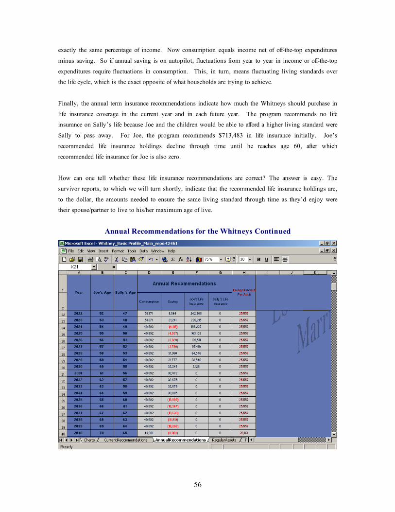
As the second next screen shot shows, recommended consumption drops again in 2024 when Sally Jr.
leaves home. It remains at the 2024 value of $40,892 until 2040, when Joe reaches age 70. Recall that we
used the Standard of Living Index to tell the program to raise the household’s living standard by 10
percent starting in 2040. In that year recommended consumption is $44,981, which is precisely 10 percent
higher than $40,892. The $44,981 recommendation is maintained through 2065, the year Joe, assuming
he survives until then, reaches 95 -- his maximum age of life. From 2066 through 2070, Sally’s last
possible year of life, recommended consumption is $28,113. Note that $44,981 is 1.6 times larger than
$28,113. This is consistent with our assumption in the Assumptions folder that two can live as cheaply as
1.6.
(There is one other reason recommended consumption can change, which we’ll discuss in more detail
below. That’s when the household is unable to have the same living standard when young as when old
without going into debt or going deeper into debt than the household is willing to accept.)
In regarding the program’s recommended changes over time in consumption expenditure, it’s important to
bear in mind that individual household members enjoy the same living standard year in and year out prior
to 2040 and a 10 percent higher living standard after 2040. Stated differently, the program adjusts
consumption recommendations in accordance with changes over time in the household’s demographic
composition, the relative cost of children, economies in shared living, and standard of living preferences.1
But each of these adjustments, except those involving desired future changes in living standard, are made in
order to preserve the living standards of individual household members.
1 If C stands for a household’s total recommended consumption expenditure and S stands for the living
standard per adult, the formula relating the two variables is given by T = S x Me , where M stands for the
the number of adults plus the sum of each child’s cost weight. If, for example, a family has two adults and two children and the equivalent cost of supporting the younger child is 70 percent of an adult and the cost
of supporting the older child is 80 percent of an adult, the cost weights are .7 and .8, and the value for M is
2 + 1.5 = 3.5. The exponent e equals the natural log of z divided by the natural log of 2, where x is the
value of the economies of shared living entered in the Assumptions folder. In the current example, we
assume that 2 can live as cheaply as 1.6, so z equals 1.6.
55
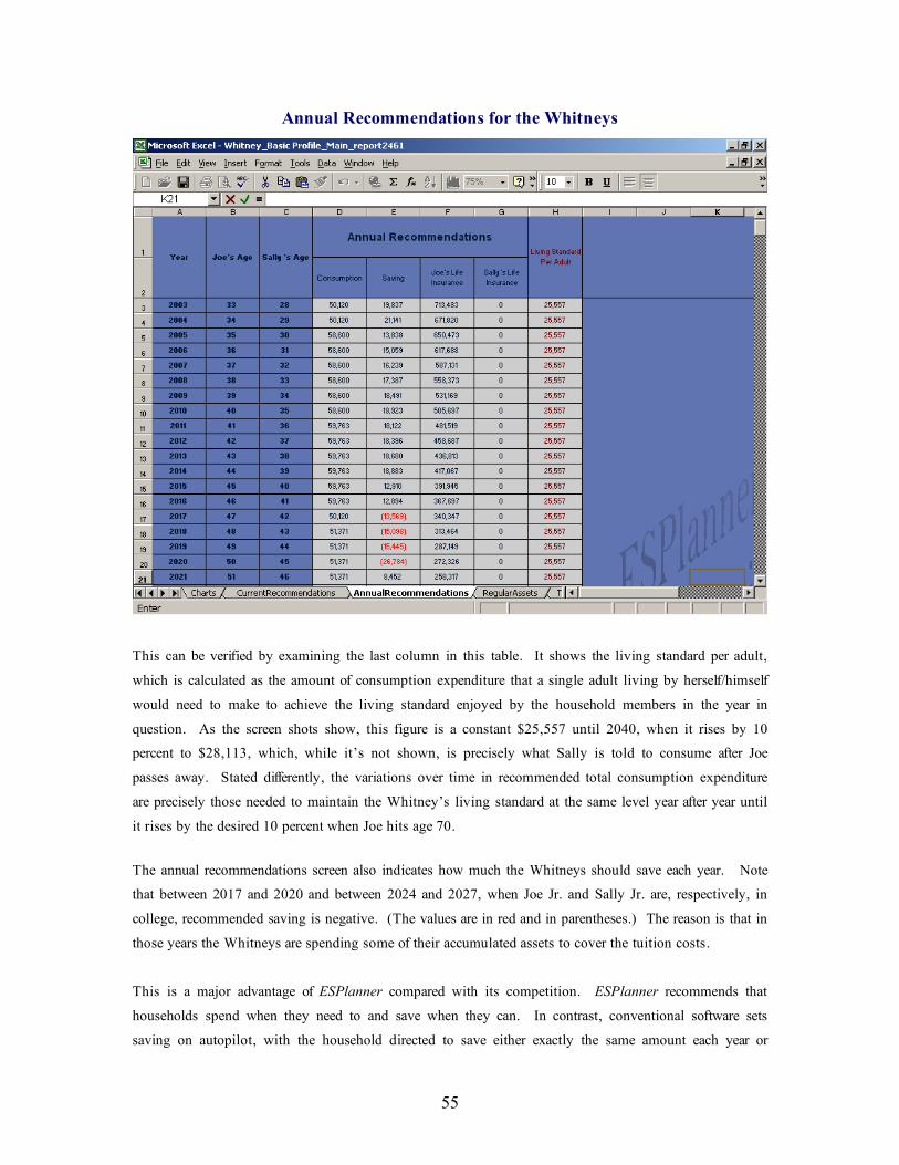
Annual Recommendations for the Whitneys
This can be verified by examining the last column in this table. It shows the living standard per adult,
which is calculated as the amount of consumption expenditure that a single adult living by herself/himself
would need to make to achieve the living standard enjoyed by the household members in the year in
question. As the screen shots show, this figure is a constant $25,557 until 2040, when it rises by 10
percent to $28,113, which, while it’s not shown, is precisely what Sally is told to consume after Joe
passes away. Stated differently, the variations over time in recommended total consumption expenditure
are precisely those needed to maintain the Whitney’s living standard at the same level year after year until
it rises by the desired 10 percent when Joe hits age 70.
The annual recommendations screen also indicates how much the Whitneys should save each year. Note
that between 2017 and 2020 and between 2024 and 2027, when Joe Jr. and Sally Jr. are, respectively, in
college, recommended saving is negative. (The values are in red and in parentheses.) The reason is that in
those years the Whitneys are spending some of their accumulated assets to cover the tuition costs.
This is a major advantage of ESPlanner compared with its competition. ESPlanner recommends that
households spend when they need to and save when they can. In contrast, conventional software sets
saving on autopilot, with the household directed to save either exactly the same amount each year or
56
exactly the same percentage of income. Now consumption equals income net of off-the-top expenditures
minus saving. So if annual saving is on autopilot, fluctuations from year to year in income or off-the-top
expenditures require fluctuations in consumption. This, in turn, means fluctuating living standards over
the life cycle, which is the exact opposite of what households are trying to achieve.
Finally, the annual term insurance recommendations indicate how much the Whitneys should purchase in
life insurance coverage in the current year and in each future year. The program recommends no life
insurance on Sally’s life because Joe and the children would be able to afford a higher living standard were
Sally to pass away. For Joe, the program recommends $713,483 in life insurance initially. Joe’s
recommended life insurance holdings decline through time until he reaches age 60, after which
recommended life insurance for Joe is also zero.
How can one tell whether these life insurance recommendations are correct? The answer is easy. The
survivor reports, to which we will turn shortly, indicate that the recommended life insurance holdings are,
to the dollar, the amounts needed to ensure the same living standard through time as they’d enjoy were
their spouse/partner to live to his/her maximum age of live.
Annual Recommendations for the Whitneys Continued

57
The Whitneys’ Spending Report
Next, let’s examine the Spending Report, provided in another worksheet in the Main Reports. The
spending report shows not only the annual recommended level of consumption expenditures, but also how
much the Whitneys will pay for housing, special expenditures, excess bequests and funerals, insurance
premiums, and retirement account contributions. Housing expenditures decline in the report as inflation
erodes the real value of mortgage payments. In 2023, the mortgage is paid off and housing expenditures
drop to $5,500 per year. The column labeled “special expenditures” shows the children’s college expenses
occurring in the correct years.
ESPlanner is designed to use your family’s home equity to cover any bequests and funeral expenses of the
last household member to pass away. That’s why the bequest and funeral expense column is labeled
“excess” bequests and funeral expenses. It’s the bequest and funeral expenses above and beyond the
amount that can be covered by available home equity. The insurance premiums are those associated with
purchasing recommended levels of life insurance coverage for Joe. And the retirement account
contributions, which in the Whitney’s case are zero, are those made by your family, not your family’s
employers. (Note that employer contributions to your family members’ retirement accounts are fully
included in calculating retirement account withdrawals.)
The Whitneys’ Total Spending Report

58
The last column in the spending report shows total spending in each year. The key question with respect
to this column of numbers is whether this recommended spending path is actually affordable. The answer,
as we’ll now see, is yes.
The Whitney’s Regular Assets Report
Were the time-path of spending shown in the Spending Report not affordable, the household would end up
in debt in the last period of the household’s possible existence. As the Whitney’s Regular Asset Report,
parts of which are copied below, indicates, this doesn’t happen. The program makes sure the Whitneys
“die broke.” This means that they spend all their resources (apart from housing equity not used to cover
Sally’s final bequest and funeral expenses), but they don’t leave any bills unpaid.
The first of the Regular Assets screen shots shown below shows that the couple spends down its assets to
send the two kids to college. The second screen shot shows that the couple dies broke; i.e., regular assets
in 2070 when Sally reaches age 95 equal zero. The Regular Assets Report is a balance sheet. The annual
change in regular assets equals that year’s saving. And saving equals income minus the sum of total
spending plus taxes.

59
The Whitneys’ Regular Assets

60
The Whitneys’ Regular Assets Continued
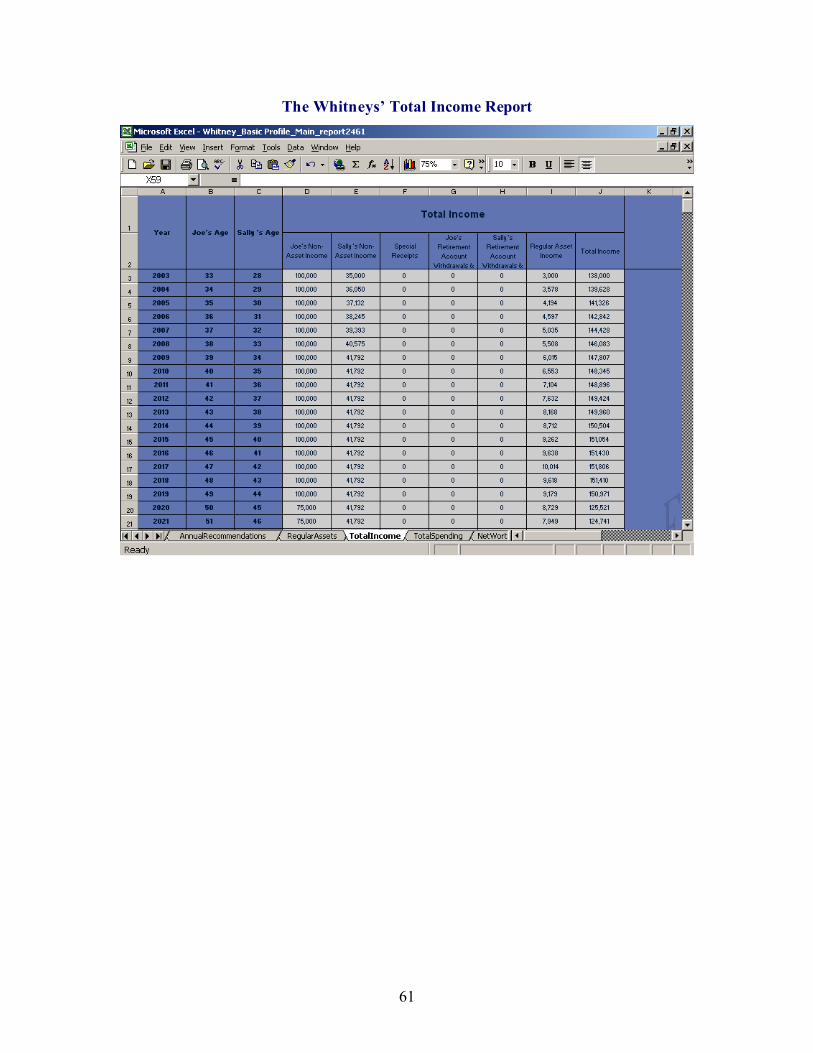
The Whitneys’ Total Income Report
The next report in Main Reports that we want to show you is the Total Income Report. This report
decomposes the household’s total income into four components – non-asset income, special receipts,
retirement account withdrawals and annuities, and income from the household’s regular assets. Non-asset
income consists of labor earnings, social security benefits, pension benefits, and regular annuities (annuities
that aren’t derived from retirement accounts).
The Whitney’s Net Worth Report
The remaining report in Main Reports shows the Whitney’s’ total net worth each year, breaking total net
worth into components. These components are regular assets, retirement account balances, home equity,
and the value of the couple’s reserve fund.
61
The Whitneys’ Total Income Report

62
The Whitneys’ Net Worth
The Whitneys’ Detai led Reports
ESPlanner’s detailed reports spell out the components of your family members’ non-asset incomes,
housing expenses, taxes, Social Security benefits, reserve fund, estates, and retirement accounts. Here are
three examples of such reports. The first of these three screen shots show that Joe’s labor income declines
at age 50 when he stops consulting. It also shows that he starts collecting Social Security retirement
benefits starting at age 65.
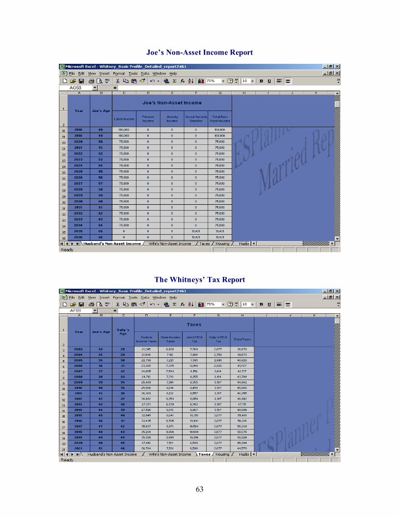
63
Joe’s Non-Asset Income Report
The Whitneys’ Tax Report

64
The Whitneys’ Housing Report
The Whitneys’ Survivor Reports
The next screen shot shows Sally’s annual recommendations as a survivor were Joe to die at the end of his
33rd
year. The first thing to notice is that Sally’s living standard is precisely the same $25,527 per
equivalent adult as she and other family members experience if Joe lives to a ripe old age. The next thing
to notice is that Sally’s recommended consumption does not rise in 2005 when Sally Jr. would otherwise
have been born; i.e., the program realizes that if Joe is deceased, Sally Jr. will not be forthcoming. The
third thing to notice is that Sally’s recommended consumption varies over time as Joe Jr. becomes more
expensive in 2011 and then leaves the household in 2017. Although it’s not shown, Sally’s recommended
survivor consumption rises by 10 percent when she reaches age 65, to ensure that she enjoys precisely the
same living standard when she’s a widow as she would had Joe not died.
The next question to ask is whether Sally, as a survivor, can actually afford the same living standard. The
answer is shown in her survivor Regular Assets report, part of which is shown below. As this report
indicates, Sally begins life as a widow with $811,320. As Joe’s Estate
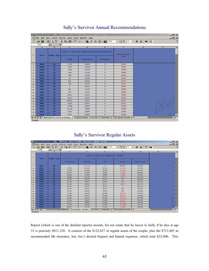
65
Sally’s Survivor Annual Recommendations
Sally’s Survivor Regular Assets
Report (which is one of the detailed reports) records, his net estate that he leaves to Sally if he dies at age
33 is precisely $811,320. It consists of the $122,837 in regular assets of the couple, plus the $713,483 in
recommended life insurance, less Joe’s desired bequest and funeral expenses, which total $25,000. This

66
shows that ESPlanner’s life insurance recommendation is, to the dollar, exactly what Sally needs to
maintain her living standard and that of Joe Jr.
In addition to the annual recommendations and regular asset reports, the other survivor reports provide
detailed information about sources of income, taxes, Social Security benefits, housing, and spending of
survivors.
Joe Retires Early
Our next goal is to show you how easy it is to use ESPlanner to determine implications for the Whitneys’
living standard of changes in financial plans and goals. Our first example involves Joe’s retiring at age 60,
rather than 65. To consider this case, we return to the Family List by clicking Show on the Family Tool
Bar. Next we select Basic Plan under Whitney. Finally, we click Save As on the Profiles Tool Bar and
enter Retire Early as the new file name. The program automatically copies all the inputs from Basic Plan
into Retire Early.
We then click on Retire Early, click Inputs, click Earnings on the folder list, select Joe, go to the earnings
grid, selected the year that Joe reaches age 60, enter zero earning for that year, and then grow those earnings
at a zero rate. This fills in earnings of zero for ages 60 and beyond. Before hitting the Create Reports
button, we do one other thing. We go to the Future Covered Earnings screen in the Social Security folder
and copy Joe’s future earnings.
Compared with the Basic Plan, the program now recommends that the Whitneys consume only $46,800 in
the current year, rather than $50,120. This entails a living standard reduction of 6.6 percent as can be
double checked by comparing the living standard per adult figures across the two sets of annual
recommendations. The program also recommends that the Whitneys save 17.1 percent more this year --
$23,233 rather than $19,837. Because Joe’s future earnings are reduced, he has less future income to
insure. Consequently, the program recommends that Joe reduce his current life insurance by close to
$100,000.

67
Joe and Sal ly Do Contingent Planning
We next demonstrate how to do contingent planning. Specifically, we return to the base case assumption
but assume that were Joe to die, Sally would choose a more demanding career and earn $75,000 each year
measured in today’s dollars. We also assume that she’d need to hire a nanny for 7 years to help take care
of the children, which would cost $15,000 per year.
To activate contingent planning, we click Show on the Family Tool Bar and return to the Whitney family
screen. There we check off contingent planning. When we click on Inputs under Basic Plan, the input
folder list appears, but with contingent planning input folders added to the list.
Since many of your family members’ contingent plans may be the same as their regular plans, the program
permits you to copy their respective regular plans into the contingent planning input fields. This can be
done by opening the Copy Center folder, checking off what regular inputs you’d like to copy to their
contingent counterparts, and then clicking Copy.
If you are running contingent planning (have activated contingent planning), it’s very important to
bear in mind that most contingent entries, such as contingent future earnings, will be zero unless
you enter alternative values. If, for example, you don’t tell the program that Sally will have
earnings if Joe dies, the program will assume she will have no earnings in that eventuality and
recommend much more life insurance than is really needed.
In this case, we copied all the inputs except Sally’s earnings, her Social Security inputs, and her special
expenditures if Joe dies. We then clicked first on Social Security and then on Special under Contingent
Planning to enter the right covered earnings for Sally and the right nanny expenses in the event Joe dies.
The new results are a lot different from the previous results with respect to Joe’s recommended life
insurance holdings. The program was recommending that Joe purchase $713,483 in life insurance. But
now that it knows that Sally will double her earnings if Joe dies, it recommends that Joe purchase only
$2,133 in life insurance.
Using the Copy Center To Do Contingent Planning

68
Check off the regular data you want to copy
as contingent inputs and then click Copy.
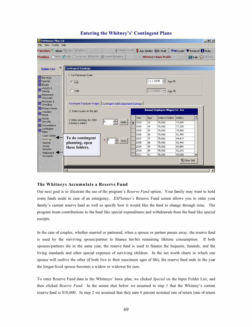
69
Entering the Whitney’s’ Contingent Plans
The Whitneys Accumulate a Reserve Fund
Our next goal is to illustrate the use of the program’s Reserve Fund option. Your family may want to hold
some funds aside in case of an emergency. ESPlanner’s Reserve Fund screen allows you to enter your
family’s current reserve fund as well as specify how it would like the fund to change through time. The
program treats contributions to the fund like special expenditures and withdrawals from the fund like special
receipts.
In the case of couples, whether married or partnered, when a spouse or partner passes away, the reserve fund
is used by the surviving spouse/partner to finance her/his remaining lifetime consumption. If both
spouses/partners die in the same year, the reserve fund is used to finance the bequests, funerals, and the
living standards and other special expenses of surviving children. In the net worth charts in which one
spouse will outlive the other (if both live to their maximum ages of life), the reserve fund ends in the year
the longer-lived spouse becomes a widow or widower for sure.
To enter Reserve Fund data in the Whitneys’ basic plan, we clicked Special on the Input Folder List, and
then clicked Reserve Fund. In the screen shot below we assumed in step 1 that the Whitney’s current
reserve fund is $10,000. In step 2 we assumed that they earn 6 percent nominal rate of return (rate of return
To do contingent
planning, open
these folders.

70
before inflation) on the fund. In Step 3 we specified that the Whitneys want to have a $13,000 fund (valued
in today’s dollars) at the end of the current year. In step 4 we assumed that 30 percent of the funds income
would be used to cover taxes. In step 5, we grew the fund by 5 percent per year. Finally, in step 6 we
specified that fund income is taxable.
When we run the Whitneys’ basic plan, but with these reserve fund information entered, recommended
consumption in the current year falls from $50,120 to $47,270. The reserve fund assets now show up in
the Net Worth Report, and net contributions to the reserve fund now show up in the Spending Report.
The Whitneys Have Retirement Accounts
Next let’s give the Whitneys current retirement account assets and assume they contribute over time to
retirement accounts. As the next four screen shots indicate, the program allows you to specify current
holdings in and future contributions to employer accounts, individual deductible accounts, and Roth IRA
accounts.
You can also tell the program when family members will stop contributing to these accounts, how much
they will contribute each year, when they will start and stop withdrawing their retirement account assets,
the fraction of their retirement account balances that will be converted to annuities at the initial date of
withdrawal, the type of annuity they will choose, and the order in which non-annuitized account balances
will be withdrawn.
The fifth screen shot in this section shows Joe’s Retirement Account Report, which tracks the evolution of
Joe’s retirement account assets, including his and his employer’s contributions to his accounts as well as
his withdrawals from his accounts. Like the regular asset report, the retirement account reports zero out at
the end showing you that all the funds and income earned on the accounts are used by ESPlanner for
meeting recommended consumption and other expenditures.
You can run your family’s plan with different retirement account contribution levels, different degrees of
annuitization, different retirement account withdrawal dates and withdrawal orderings, different annuity
designs, etc. Each time you run the program, check the resulting living standard generated by the program.
Since the goal is to maximize your family’s living standard, you’ll quickly be able to determine how
retirement accounts can help you meet that goal.
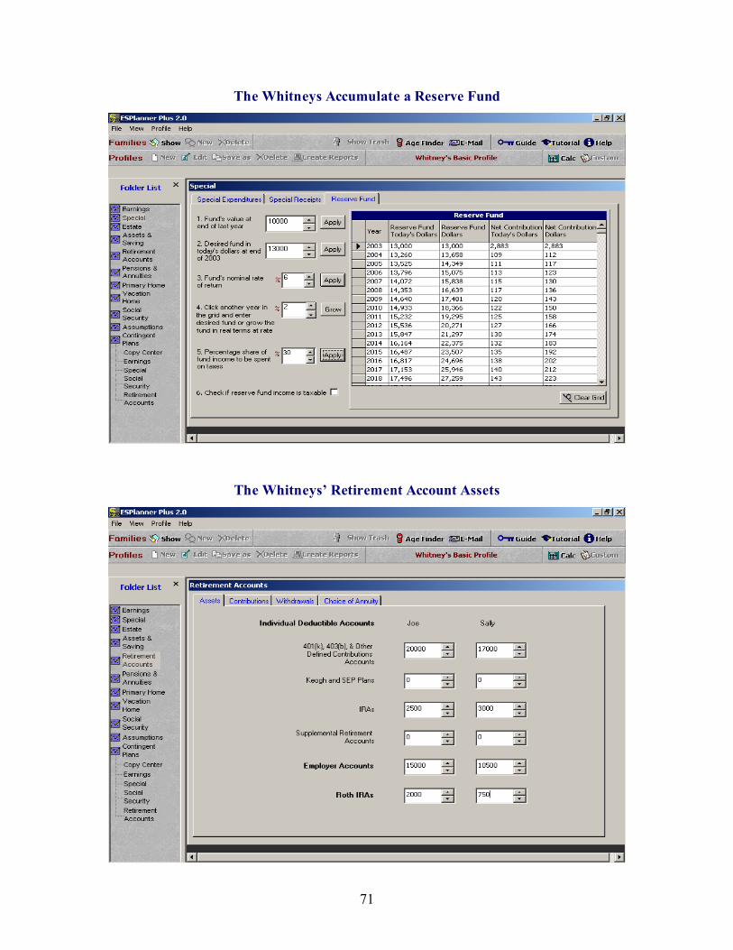
71
The Whitneys Accumulate a Reserve Fund
The Whitneys’ Retirement Account Assets
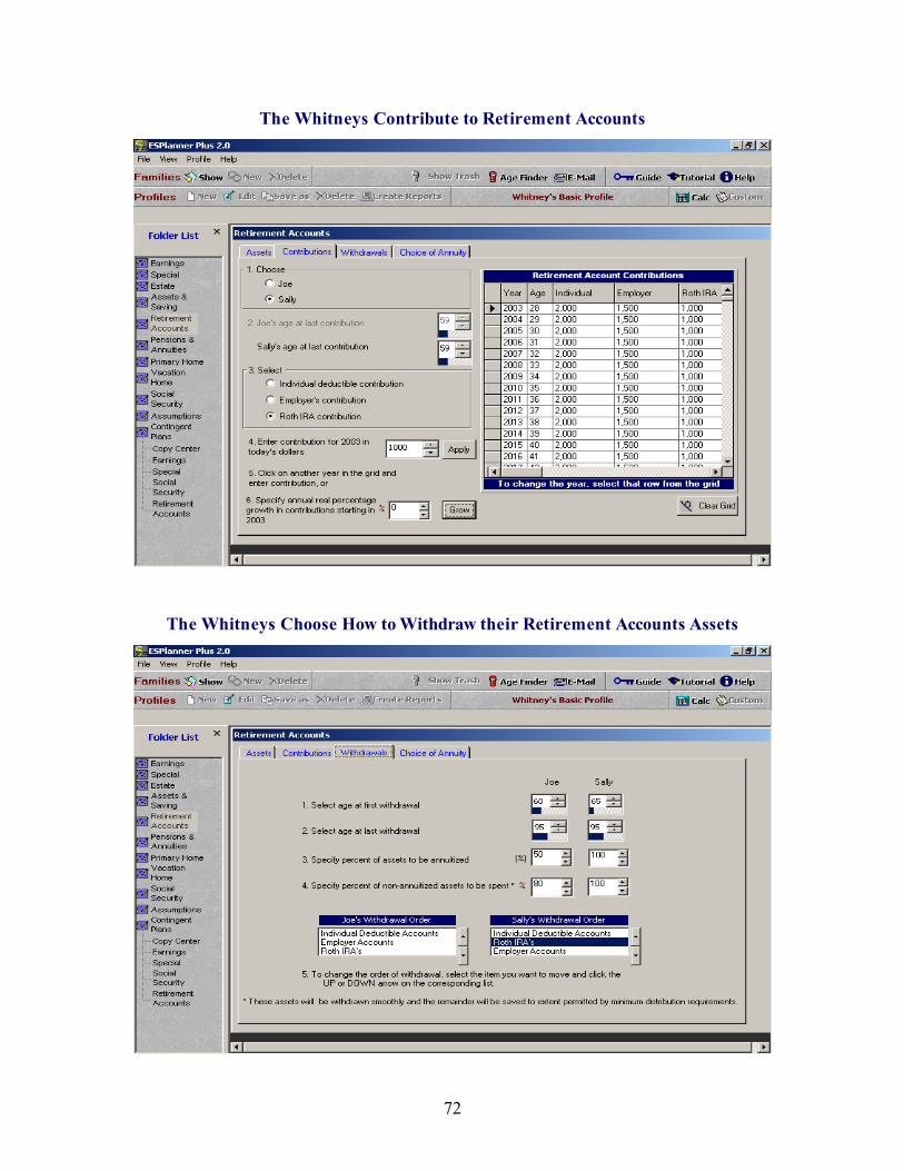
72
The Whitneys Contribute to Retirement Accounts
The Whitneys Choose How to Withdraw their Retirement Accounts Assets

73
The Whitneys Design their Retirement Account Annuities

74
The Evolution of Joe’s Retirement Account
Joe and Sal ly Expect to Receive a Very Large Inheritance
Let’s now assume that Joe and Sally expect to receive a very large inheritance, say $5 million, but not for
10 years. Since they are unable to borrow against this future receipt, the couple is strapped for cash or, in
the language of economists, borrowing or liquidity constrained and cannot enjoy as high a living standard
in the next 10 years as they will thereafter.
ESPlanner deals with borrowing constraints by generating the smoothest living standard path for your
family without putting it into debt or, if it is able to borrow, without putting it into more debt than the
borrowing limit specified in the Economic Assumptions folder.
We enter Joe’s and Sally’s expected inheritance in the Special Receipts screen in the Special input folder.
The spending report for this case is shown below. As you can see, recommended consumption jumps
dramatically in 2013 when the couple receives their inheritance. Recommended saving jumps as well since
the couple saves the vast majority of what it inherits in order to enjoy a higher living standard in future
years as well. Note also that in the ten years prior to receiving an inheritance, the program smoothes the

75
couple’s living standard as well. This is a key feature of ESPlanner’s consumption smoothing.
ESPlanner not only smoothes your family’s living standard over its entire life cycle to the maximum
extent possible given its borrowing limits, it also smoothes your family’s living standard during each sub
interval of its life cycle.
Recommended Consumption When Joe and Sally Inherit
+
Asset Accumulation When Joe and Sally Inherit
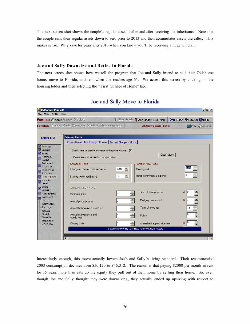
76
The next screen shot shows the couple’s regular assets before and after receiving the inheritance. Note that
the couple runs their regular assets down to zero prior to 2013 and then accumulates assets thereafter. This
makes sense. Why save for years after 2013 when you know you’ll be receiving a huge windfall.
Joe and Sal ly Downsize and Retire in Florida
The next screen shot shows how we tell the program that Joe and Sally intend to sell their Oklahoma
home, move to Florida, and rent when Joe reaches age 65. We access this screen by clicking on the
housing folder and then selecting the “First Change of Home” tab.
Joe and Sally Move to Florida
Interestingly enough, this move actually lowers Joe’s and Sally’s living standard. Their recommended
2003 consumption declines from $50,120 to $46,312. The reason is that paying $2000 per month in rent
for 35 years more than eats up the equity they pull out of their home by selling their home. So, even
though Joe and Sally thought they were downsizing, they actually ended up upsizing with respect to

77
overall long-term housing expenditures. The housing report, copied below, shows what happens to their
housing expenditures from this move.
The Impact on Joe and Sally of “Downsizing” their Home
Joe and Sal ly Run Monte Carlo Simulations
The next three screen shots help you understand how to run Monte Carlo simulations assuming you have
a) purchased ESPlannerPlus and b) activated Monte Carlo on the Family Information screen.
The program’s Monte Carlo calculations begin with a dynamic program that determines how much the
household should consume each period given all the different levels of regular and retirement account assets
it could possibly have in that period. This dynamic program takes into account that higher (lower) regular
and retirement account asset levels mean higher (lower) taxes (depending on the year in question).
The dynamic program assumes that households, at any point in time, will base their consumption decision
on ESPlanner’s recommendation. Once this set of consumption functions (one for each future period) is
generated, the program randomly selects 500 time paths of annual asset returns. Each time path of returns

78
is then used in conjunction with the family’s portfolio choices to figure out what rate of return the
household will earn each period on its regular and retirement account portfolios.
For each of the 500 time paths of portfolio returns, the Monte Carlo simulations begin by using the
household’s initial regular and retirement account asset levels (the initial state variables) to determine,
based on the initial period consumption function, how much the household should consume in that period.
This decision, in turn, determines how much the household saves and, given the portfolio returns, how
much regular and retirement account assets the household will have at the beginning of the second period.
These second-period asset levels are then inputted into the second-period consumption function to
determine second-period consumption, and so on. The simulation proceeds in this manner through the last
period a household member could be alive.
In the process of calculating the entire time path or trajectory of consumption associated with each of the
500 time paths of randomly drawn returns, we also determine the associated time paths of retirement and
regular asset levels, income levels, saving levels, etc. After each of the 500 trajectories of all variables has
been determined, we do two things. First, we show the percentile distribution of outcomes for the
household’s living standard, income, and asset levels in each future year. Second, we rank the 500
trajectories based on the present value of consumption and display the trajectories for the household’s
living standard, income, and asset positions associated with the fifth lowest, 25th lowest, 50
th lowest, 75
th
lowest, and 95th
lowest present values of consumption. We refer to these as lowest, low, middle, high, and
highest trajectories.
In the following two screen shots we assume that Joe and Sally have a favorite stock, XYZ Corp., and
show you how to enter that asset in the first, Build Portfolio, screen of the Monte Carlo folder. In the
second of these two screen shots, we renamed Portfolio 2 as “Hot Tip,” we removed the non-cash assets
from the Hot Tip portfolio, and then selected XYZ Corp. from the asset grid. Next, we set the asset
percentage at 50 percent, and then used the Add button to add XYZ Corp. to the Hot Tip portfolio. Then
we selected large cap stocks and added 50 percent holdings of that asset as well to the Hot Tip portfolio.
We next renamed Portfolios 3 and 4 to “Play It Safe” and “U.S. Stocks” and then used the Remove and
Add buttons to define those portfolios as consisting, respectively, of 100 percent inflation-indexed bonds
and 100 percent in large cap U.S. equity. Finally, as the next screen shot shows, we told the program that
through 2040 the couple wants to a) hold only its Hot Tip portfolio when it comes to its regular assets, b)
hold only its Play It Safe portfolio in Joe’s retirement account and c) hold its U.S. Stocks portfolio in
Sally’s retirement accounts for 10 years and then switch to Play It Safe. After 2040, the couple wants to
hold only the Play It Safe portfolio.
The next three screen shots show examples of the Monte Carlo reports. In this run, we’ve given Joe and
Sally $50,000 in initial retirement account assets and assumed no future contributions. The first of the

79
three screen shots show the percentile distribution of the couple’s living standard each year as they age.
The second shows very low, low, middle, high, and very high trajectories of the couple’s total income.
The third shows a tabular display of the percentile distribution of the couple’s regular assets.
Once you consider these results, you may want to adjust your portfolio decisions. Note that in the case we
present, once Joe and Sally switch in 2040 to the Play It Safe portfolio, their income trajectories show no
variability from one period to the next. This illustrates that the program can be used to deliver different
degrees of income, asset, and living standard variability when young and when old.
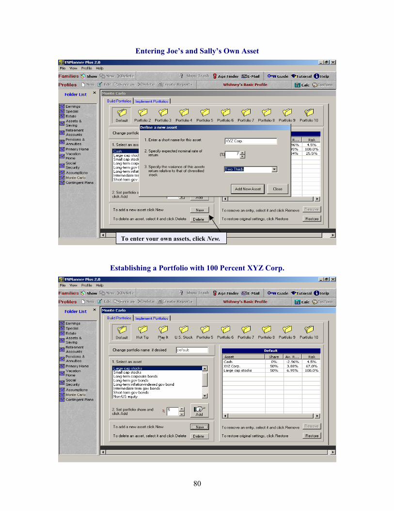
80
Entering Joe’s and Sally’s Own Asset
Establishing a Portfolio with 100 Percent XYZ Corp.
To enter your own assets, click New.
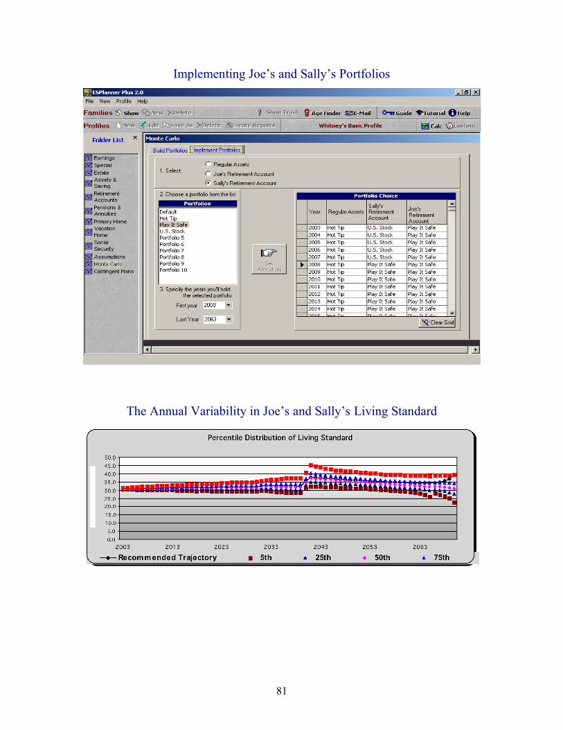
81
Implementing Joe’s and Sally’s Portfolios
The Annual Variability in Joe’s and Sally’s Living Standard

82
Illustrating Alternative Income Trajectories
The Percentile Distribution of Joe’s and Sally’s Regular Assets