ESAPESAP--95 Version 2.01R95 Version 2.01R

User Manual User Manual and and

Tutorial GuideTutorial Guide

USDA USDA -- ARS ARS George E. Brown, Jr., Salinity LaboratoryGeorge E. Brown, Jr., Salinity Laboratory

Research Report No. 146Research Report No. 146

June 2000June 2000

ii

ESAP-95 Version 2.01R User Manual and Tutorial Guide

Scott M. Lesch, James D. Rhoades, and Dennis L. Corwin

Research Report No. 146

June 2000

United States Department of Agriculture

Agricultural Research Service

George E. Brown, Jr., Salinity Laboratory

Riverside, California

iii

DISCLAIMER

The information in, and/or ESAP-95 software package associated with this document has been funded and developed by the United States Department of Agriculture, Agriculture Research Service, at the George E. Brown, Jr., Salinity Laboratory. Partial funding for the software package from the United States Bureau of Reclamation is also gratefully acknowledged. Both this user manual and the ESAP-95 software associated with this manual are to be considered public domain software, and as such may be used and copied free of charge. Although the authors of this software have endeavored to produce accurate and error free program code, this software (including instructions for its use) is provided "as is" without warranty, expressed or implied. Furthermore, neither the authors nor the United States Department of Agriculture warrant, guarantee, or make any representations regarding the use, or the results of the use of, or instructions for use of this software or manual in terms of applicability, reliability, accuracy, or correctness. The use and application of this software and manual is the sole responsibility of the user. The mention of any trade names or commercial products is for the convenience of the user and does not imply any particular endorsement by the United States Department of Agriculture or its agents.

iv

Technical Abstract Lesch, S. M., J. D. Rhoades, and D. L. Corwin. 2000. The ESAP-95 version 2.01R user manual

and tutorial guide. Research Report No. 146. USDA-ARS, George E. Brown, Jr., Salinity Laboratory, Riverside, California.

This manual describes and documents a series of site selection and salinity modeling software programs, collectively known as the ESAP-95 software package (Release version 2.01R), developed for the analysis and prediction of soil salinity from conductivity survey information. It is designed to be used both as a software reference text and tutorial guide. The ESAP-95 software package currently contains three programs: ESAP-RSSD, ESAP-Calibrate, and ESAP-SaltMapper. The ESAP-RSSD program is designed to generate optimal soil sampling designs from bulk soil electrical conductivity survey information. The ESAP-Calibrate program is design to estimate both stochastic (regression model) and deterministic (soil theory based) calibration equations; i.e., the equations which are ultimately used to predict the spatial values of one or more soil variables from conductivity survey data. The final program, ESAP-SaltMapper, can be used to produce high quality 1D or 2D graphical output of conductivity survey data and/or predicted soil variables. This manual describes and documents to implementation and use of each of these three programs in detail.

v

Table of Contents 1.0 Introduction 1 1.1 General conductivity / salinity assessment techniques 1 1.2 The ESAP-95 software package description 2 1.3 Software installation directions 4 1.4 ESAP-95 software training files 6 1.5 ESAP-95 software package development information 7 2.0 ESAP-95 Software Overview 9 2.1 Software package design 9 2.2 Data input / output 11 2.3 An overview of the 3 main ESAP program menus 12 2.4 Supported surveying techniques and applications 15 2.5 On-line help documentation 15 3.0 ESAP-RSSD Software Program 17 3.1 ESAP-RSSD program overview 17 3.1.1 Program description 17 3.1.2 Navigating the main menu 19 3.2 Data file input specifications 22 3.2.1 Creating a project and field ID 23 3.2.2 Reading in survey data 23 3.2.3 Practice module 26 3.3 Data visualization 28 3.3.1 Description of graphical techniques 28 3.3.2 Navigating the graphics menu 31 3.3.3 Invoking the GI and CT windows 34 3.3.4 Practice module 35 3.4 Data analysis 42 3.4.1 Basic statistics 42 3.4.2 Using the decorrelation / validation algorithms 43 3.4.3 Additional transect file validation options 44 3.4.4 Practice module 45

vi

3.5 Generating sampling designs 47 3.5.1 The manual sample site selection procedure 49 3.5.2 Generating spatial response surface (SRS) sampling designs 49 3.5.3 Practice module 51 3.6 Data Output 52 3.6.1 Text output 52 3.6.2 Graphical output 53 3.6.3 Creating an output *.svy data file 53 3.6.4 Practice module 53 4.0 ESAP-SaltMapper Software Program 59 4.1 ESAP-SaltMapper program overview 59 4.1.1 Program description 59 4.1.2 Navigating the main menu 60 4.2 Data input and manipulation 62 4.2.1 Setting the current project and importing data 62 4.2.2 Renaming columns 63 4.2.3 Creating new data columns 63 4.2.4 Displaying basic column statistics 65 4.2.5 Practice module 65 4.3 Creating 1D line plots 66 4.3.1 Definition of a 1D line plot 66 4.3.2 Navigating the 1D line plot menu 67 4.3.3 Line plot initialization options 68 4.3.4 Adding a title, axis labels, and a legend to the plot 69 4.3.5 Practice module 70 4.4 Creating 2D raster maps 71 4.4.1 About the raster map creating process 71 4.4.2 Using the on-screen interpolation controls 72 4.4.3 Navigating the raster map menu 74 4.4.4 Setting the map variable specification options 76 4.4.5 Practice module 77

vii

4.5 Migrating data out of the ESAP-SaltMapper program 79 4.5.1 Creating and saving ASCII text files 80 4.5.2 Practice module 80 5.0 ESAP-Calibrate Software Program 81 5.1 ESAP-Calibrate program overview 81 5.1.1 Program description 81 5.1.2 Navigating the main menu 84 5.2 Importing previously saved ESAP data files 87 5.2.1 Importing ESAP-RSSD survey data files 87 5.2.2 Importing ESAP-Calibrate profile data files 88 5.2.3 Practice module 89 5.3 Importing new data files 90 5.3.1 The two types of laboratory profile data 90 5.3.2 Importing data (file type / column structure specifications) 92 5.3.3 Practice module 94 5.4 Editing and validating new profile data 96 5.4.1 Validating new laboratory profile data 96 5.4.2 Editing laboratory profile data 97 5.4.3 Practice module 98 5.5 Deterministic salinity conversion modeling 99 5.5.1 How does a deterministic conversion work 99 5.5.2 Navigating the DCS menu 100 5.5.3 Setting the conductivity to ECa input parameters 101 5.5.4 Setting the secondary soil input parameters 103 5.5.5 Practice module 104 5.6 Performing a 1D profile analysis 106 5.6.1 What is a 1D profile plot 106 5.6.2 Navigating the 1D profile menu 107 5.6.3 Initializing a 1D profile plot for display 109 5.6.4 Practice module 110

viii

5.7 Performing a 2D standard correlation analysis 113 5.7.1 What is a standard correlation analysis 114 5.7.2 Navigating the standard correlation analysis menu 114 5.7.3 Practice module 117 5.8 Performing a DPPC correlation analysis 119 5.8.1 What is a DPPC profile data correlation analysis 119 5.8.2 Description of the DPPC model 120 5.8.3 Using the DPPC - PDCA window 122 5.8.4 Understanding the DPPC summary report 124 5.8.5 DPPC data plots 128 5.8.6 Navigating the DPPC graphics menu 129 5.8.7 Practice module 131 5.9 Spatial Regression modeling (Stochastic Calibration) 133 5.9.1 What is a stochastic calibration model 133 5.9.2 Navigating the SCM menu 134 5.9.3 Response variable specification window 137 5.9.4 Navigating the PRV graphics menu 139 5.9.5 Specifying the calibration model parameters 140 5.9.6 Understanding the model parameter options 142 5.9.7 Estimating the calibration model 146 5.9.8 Practice module 1 146 5.9.9 Viewing 2D prediction scatter plots 148 5.9.10 Calculating field summary statistics 150 5.9.11 Using the salt tolerance window 151 5.9.12 Saving your output predictions 152 5.9.13 Practice module 2 153 5.9.14 Advanced options: Net flux testing 156 5.9.15 Advanced options: Advanced modeling information 158 6.0 References 160

1

1.0 Introduction 1.1 General Conductivity / Salinity Modeling and Assessment Techniques Accurate soil salinity assessment is needed for the design of efficient agricultural management practices and irrigation water allocation strategies. Fortunately, the ability to diagnose and monitor field scale salinity conditions has been significantly improved through the use of both four-electrode and electromagnetic induction (EM) survey instruments. Within the last 15 years, the adaptation of four-electrode and EM sensors for soil electrical conductivity measurement has greatly increased both the speed and reliability of salinity reconnaissance survey work. The efficient use of conductivity signal information requires the conversion of apparent soil conductivity (ECa) into soil salinity (ECe). A significant amount of research in recent years has been directed towards developing efficient conversion techniques (Williams and Baker, 1982; McNeill, 1986, 1980; McKenzie et. al., 1989; Rhoades and Corwin, 1990; Rhoades et. al., 1999, 1991, 1990, 1989; Rhoades, 1996, 1992; Slavich, 1990; Cook and Walker, 1992; Diaz and Herrero, 1992; Yates et. al., 1993, Lesch et. al., 1998, 1995a,b, 1992). These conversion techniques can generally be classified into one of two methodological approaches; (1) deterministic, and (2) stochastic. In the deterministic approach, either theoretically or empirically determined models are used to convert conductivity into salinity. Deterministic models are "static"; i.e., all model parameters are considered known and no soil sample (soil salinity) data needs to be collected during the survey. However, these models typically require knowledge of additional soil properties (e.g., soil water content, texture, temperature, etc.). In the stochastic approach, statistical modeling techniques such as spatial regression or cokriging are used to directly predict the soil salinity from conductivity survey data. In this latter approach, the models are "dynamic"; i.e., the model parameters are estimated using soil sample data collected during the survey. A unified, deterministic model for describing the relationship between soil electrical conductivity and soil salinity was introduced in Rhoades et al., 1989. This model, which is now commonly referred to as the Dual Pathway Parallel Conductance (DPPC) equation, described how soil salinity could be estimated from measurements of soil conductivity, texture, bulk density, water content, and temperature. Additionally, robust field measurement techniques were developed and described for acquiring the above conductivity and soil physical properties. In Lesch et. al., 1995a,b, a comprehensive methodology was introduced for carrying out a field scale salinity survey using a stochastic/dynamic modeling approach. This methodology centered around the use of spatial regression models for predicting soil salinity from conductivity survey data, when knowledge of the corresponding soil

2

physical properties was either unavailable or too impractical to collect. These models were shown to have a number of important advantages over other statistical modeling approaches, including (1) they facilitated the use of rapid, mobile conductivity surveying techniques, (2) they could be estimated using a very limited number of soil samples, (3) they could make both point and conditional probability estimates, (4) they could be used to test for changes in the geometric mean field salinity level over time, and (5) they were shown to be theoretically equivalent to cokriging models, provided the regression model residuals are spatially independent. There are both advantages and disadvantages to using either modeling approach. For example, stochastic models are usually more accurate than deterministic models when the secondary soil properties are not known across all the survey sites. However, because stochastic models are dynamic, some soil samples must be acquired during each survey expedition. Additionally, these models also tend to be both time and location dependent. On the other hand, deterministic models are (at least in theory) both time and location independent, and these types of estimation techniques do not require calibration salinity data. But deterministic techniques do require accurate secondary soil property information at every survey site, and hence are not commonly well suited for use with automated assessment equipment, etc. This manual describes and documents a series of site selection and salinity modeling software programs contained within the ESAP-95 Software Package (release version 2.01R). The modeling techniques incorporated into this salinity software are based on the stochastic and deterministic modeling methodologies described in Lesch et al., 1995a, 1995b and Rhoades et al., 1999, 1997, and 1989. These methodologies represent efficient and practical field scale salinity estimation and prediction techniques, and the ESAP-95 Software Package has been designed to help you appropriately use these techniques on your own conductivity survey data. 1.2 The ESAP-95 Software Package Description (Version 2.01R) The ESAP-95 Software Package you are about to use currently contains three programs: ESAP-RSSD, ESAP-Calibrate, and ESAP-SaltMapper. The ESAP-RSSD program is designed to generate optimal soil sampling designs from conductivity survey information. The ESAP-Calibrate program is design to estimate both stochastic (regression model) and deterministic (soil theory based) calibration equations; i.e., the equations which you will ultimately use to predict the spatial values of one or more soil variables from your conductivity survey data. The final program, ESAP-SaltMapper, can be used to produce high quality 1-D or 2-D graphical output of your conductivity survey data and/or predicted soil variables. Most importantly, all three programs have been designed to work together in a seamless and efficient manner, and each program employs a simple, easy to learn graphical user interface.

3

Each program in this ESAP Software package contains a number of features designed to help you perform the various components of your soil salinity assessment process, as described below: ESAP-RSSD (Response Surface Sampling Design software) Used to generate optimal sampling designs for stochastic calibration models based on conductivity survey data. The following capabilities listed below have been incorporated into the RSSD program: a) ability to process grid or transect data; i.e., can be used to process EM-38, EM-31,

Verris 3100, or Mobile 4-Electrode types of signal data b) ability to handle arbitrarily large survey sizes (up to 10,000 sites per field) c) allows for the interactive display and validation of signal data d) ability to handle either 1 or 2 signal readings per survey site e) can be used to generate calibration sample sizes of 6, 12, or 20 sites per field, or

allow user to enter and record a custom sampling design f) can adjust the sampling design based on signal variability (i.e., a transition

analysis) ESAP-Calibrate (Conductivity to Salinity Calibration software) Used to convert conductivity survey data to soil salinity via either stochastic calibration or deterministic techniques (i.e., direct multiple linear regression estimation and/or the Dual Pathway Parallel Conductance equation). Additional capabilities currently include: a) ability to use stochastic calibration models to predict levels of secondary soil

properties (provided secondary sample data has been acquired) b) ability to use deterministic DPPC model to estimate theoretical strength of

correlations between raw conductivity and salinity, SP, volumetric H2O, and/or other secondary sample data which may have been acquired during the sampling process

c) ability to produce 1D profile data graphs and perform bivariate profile data correlation analysis

d) ability to fully automate the stochastic calibration (regression modeling) process ESAP-SaltMapper (1-D Transect and 2-D raster mapping software) Used to generate 1-D transect and 2-D raster maps of raw conductivity, estimated soil salinity, and/or estimated secondary soil physical properties (i.e., designed accept input files from either ESAP-RSSD or ESAP-Calibrate).

4

Figure 1.1 shows the software program flowchart for the ESAP-95 Software Package. As shown in figure 1.1, the ESAP-RSSD program should be used first to process your conductivity survey data. The ESAP-Calibrate program can then be used to import and process your soil sample data, and calibrate this soil data to the conductivity survey data. Additionally, the ESAP-SaltMapper program has been designed to produce graphical output of either your processed conductivity data or predicted soil properties. Chapter 2 of this user guide discusses the data file input requirements and output file specifications in detail. 1.3 Software Installation Directions If you are installing the ESAP-95 Software Package from floppy disks then insert disk #1 into you're a drive and click on the Windows Start button. In the dialog box, type a:\setup.exe, click on the Run button, and then follow the on-screen directions. If you are installing a down-loaded copy from the Internet then move to the folder which contains the down-loaded program code, locate the setup.exe program, and then double-click on this program to initiate the installation procedure. If you have previously installed an earlier version of the ESAP-95 Software Package (i.e., a 2.00 or 2.01 Beta version), then be sure to read the "Important Notes for Re-Installs" listed at the end of section 1.3. The only option you will be asked to specify during the installation procedure is the installation sub-directory location. The default location will be a sub-directory called US_Salinity_Lab\esap2. We recommend that you use this sub-directory unless you have a good reason to choose another location (note: ESAP-95 will automatically create this sub-directory if it does not already exist). Please note that if you have other background programs running during the installation process, then ESAP-95 may not install properly. If you encounter an error message which states "file access error occurred" (or something similar) then you probably have some type of background program running on your Windows system which needs to be shut down before the installation process can work correctly. (This error will occur when another program using one or more ".dll" or ".ocx" files which ESAP-95 is attempting to install. This usually means that you already have the dll or ocx file in question, hence you could choose to ignore this error and continue with the installation process. However, we recommend that you first try to locate and shut down the background program which is causing this error. Assuming that you use the default installation location, the sub-directory structure shown on the next page will exist on your computer once the installation process finishes:

5

C: --- US_Salinity_Lab | |--- esap2 | |--- bitmap | |--- data | | | |--- Training1 | |--- Training2 | |--- demo_input_files | |--- helpdocs All ESAP-95 software programs will reside in the esap2 directory. Additionally, the bitmap, data, demo_input_files, and helpdocs sub-directories located off the esap2 directory are used by the software programs for storing and/or retrieving various data files. In particular, the helpdocs sub-directory contains all of the on-line help documentation, the bitmap sub-directory can be used to store any graphical (bitmap) files created by any ESAP-95 graphical procedures (created in either the ESAP-Calibrate or ESAP-SaltMapper programs), and the demo_input_files sub-directory contains some demonstration input data files for use with the ESAP-RSSD program. Likewise, the data sub-directory is used by each program for the storage and/or retrieval of all survey project data files. In ESAP-95, different survey projects can be created to hold different sets of survey data; these projects are actually just sub-directories created off the data directory. The Training1 and Training2 sub-directories are simply two project directories which contain demonstration input data for use in the ESAP-Calibrate program. Important Notes for Re-Installs: If you have previously installed an earlier version of the ESAP-95 software package (i.e., a Beta version), then you should follow the steps shown below: (a) BACK-UP YOUR DATA FILES! This can be done by inserting a blank disk into

the A drive and copying the "C:\US_Salinity_Lab\esap2\data" subdirectory onto this disk. By doing this, you will automatically create a back-up copy all of your unique project directories (located off the "\data" directory) on the floppy disk.

(b) Un-install your current beta ESAP software version. This should be done by

selecting START > Settings > Control Panel and then clicking on the Add/Remove Programs icon. Next, highlight the currently installed ESAP software, click on the "Remove" software command button, and then follow the on-screen directions.

6

(c) Install the latest version of ESAP-95. After the installation process is finished, you can then restore your project directories by simply copying these sub-directories back into the data directory.

Important Notes for Windows NT Users: The ESAP-95 Software package will operate properly on an NT platform, although it was not specifically designed for such an operating system. (You can install it in the same manner as you would on a 95/98 system platform). However, the default text editor used by ESAP (write.exe) needs to be reset each time you run the software if you wish to view any output text files. You can reset the text editor using the Help > ESAP Interface Controls > ReSet Default Text Editor menu commands located within the main RSSD, Calibrate, and SaltMapper program menus. To locate the write.exe program in NT, look in the C:\Winnt\system32 subdirectory. (You can also reset ESAP to use a different text editor, if desired.) 1.4 ESAP-95 Software Training Files There are 3 demonstration conductivity survey files which are automatically installed by the ESAP setup program (into the "esap2\demo_input_files" subdirectory). These represent demonstration files which can be used with the ESAP-RSSD software program. In order to read these files into the ESAP-RSSD software, you need to know their format (i.e., what sort of information each file contains). This format information is given below: Number Site ID Type of of Signal Column Conductivity File Name File Type Columns Present Signal Data bwd101p.dat Transect 2 no EM-38 hol31.dat Grid 1 no EM-31(vertical) frank1.mws Transect 1 no USSL Mobile Wenner In addition to the above demonstration conductivity survey files, there are 2 demonstration training projects which are automatically installed by the ESAP setup program (into the "esap2\data\Training1" and "esap2\data\Training2" subdirectories). These projects contain 3 files each: an ESAP-RSSD processed survey (*.svy) file, and ESAP-Calibrate processed profile (*.pro) file, and a soil sample data file (used to create the profile data file). These *.svy and *.pro data files can be imported into the ESAP-Calibrate program and used to explore the various program modeling and analysis features (refer to sections 5.2 and 5.3 of this manual for more details on how to import these files).

7

The format for each soil sample data file (used to create the ESAP *.pro profile data files) is listed below. sk13_97.lab (DPPC type format) bwd_10296.lab (DPPC type format) column 1: site number column 1: site number column 2: sample depth (m) column 2: sample depth (m) column 3: ECe (dS/m) column 3: ECe (dS/m) column 4: SP (%) column 4: SP (%) column 5: water content (% grav) column 5: water content (% grav) column 6: SAR (unitless) column 6: bulk density (g/cm3) column 7: Boron (ppm) column 7: % Clay (%) 1.5 ESAP Software Package Development Information The ESAP-95 Software package has been developed for the Windows operating system (95/98/NT). The 2 people responsible for developing ESAP-95 are: Scott M. Lesch Principal Statistician & Lead Programmer Analyst [statistical methodology / software design and development] James D. Rhoades Research Soil Scientist & past Laboratory Director [soil theory & methodology / salinity measurement theory] Additionally, a number of other personal at the United States Salinity Laboratory have either directly or indirectly supported the development of this software package through their work efforts. Those deserving special mention include Dennis Corwin (Lead Assessment Soil Scientist), Robert LeMert and Nahid Vishteh (Assessment Research support personal) and Jessica Lin (software support). Partial funding for the development of this software package from the United States Bureau of Reclamation is gratefully acknowledged.

8

Figure 1.1 ESAP-95 software bundle: program flowchart.

Program Flowchart

(input data) conductivity survey data ↓ (input data) ESAP-RSSD calibration sample data ↓ ↓ (output data) → ESAP-Calibrate *.svy data file ↓ ↑↓ ↓ ↓ (input / output data) ↓ *.pro data file (output data) ↓ *.prd data file ↓ ↓ ↓ ↓ ESAP-SaltMapper ↓ ↓ (output) (output) graphics ASCII data output

9

2.0 ESAP-95 Software Overview 2.1 Software Program Design As explained in chapter 1, the ESAP-95 software package has been designed to help you perform field scale salinity estimation and prediction from soil conductivity survey data. However, to make effective use of this software package, you first need to have a basic understanding of how a salinity survey is normally performed. Once you acquire a feel for the steps involved in a typical salinity survey, you will find the ESAP-95 software programs much easier to use. In general, a soil conductivity based field salinity survey is carried out in four steps. In the first step, a detailed grid of apparent soil conductivity is acquired across the survey area of interest (typically an individual field). Once this conductivity data has been acquired, soil samples from a limited number of sites within the survey area are then collected. The locations of these sample sites are usually based upon an analysis of the acquired soil conductivity data (this is referred to as "target" or "model based" sampling). This sample site selection and acquisition process represents the second step in the survey. After the soil samples are removed from the field, they are generally sent to a laboratory and analyzed for salinity content (and/or any other soil chemical or physical quantities of interest). This laboratory data can then be compared to the measured soil conductivity data acquired at the corresponding sample sites, and used to "calibrate" the conductivity data. In other words, a mathematical or statistical calibration model can be estimated using the survey and soil sample data associated with the sample site locations. This calibration modeling represents the third step in the salinity survey process. Once such a model had be estimated, it is in turn used to predict the soil salinity levels at all of the remaining (non-sampled) conductivity survey sites across the field. Maps of this prediction salinity data are then created, displayed, and studied. Such a model may also be used to make other types of predictions, such as the average salinity level within the field, or the expected degree of crop loss due to the salinity levels, etc. In most situations, the calculation, display, and interpretation of the predicted salinity data represents the fourth step in the salinity survey process. Given the above scenario, we can summarize a typical salinity survey process as shown on the next page:

10

Step Component Description 1 signal processing the collection of the conductivity survey data 2 soil sampling the collection of calibration soil sample data 3 data modeling the analysis of the soil sample data, and the development of the calibration equation 4 salinity prediction the calculation, display, and interpretation of the predicted soil salinity data The programs in the ESAP-95 Software Package have been developed around these four survey steps. The ESAP-RSSD program is designed to perform the first two steps of the survey process. In other words, you use the ESAP-RSSD program to process your soil conductivity data and generate your sampling design. Likewise, the ESAP-Calibrate program has been designed to help you perform step three, and most of step four. This program can be used to estimate stochastic (i.e., statistically based) calibration models which will in turn use your conductivity survey data to make both individual site and field average salinity predictions. The ESAP-Calibrate program can also be used to analyze various relationships within your acquired laboratory sample data, and/or convert conductivity data into estimated salinity information using deterministic modeling techniques. Finally, the ESAP-SaltMapper program can be used to display the predicted spatial salinity data; i.e., to generate 2D salinity maps and/or 1D salinity transect plots. (In other words, this program can be used to perform the "display" component of the fourth step.) ESAP-SaltMapper can also be used to display the acquired soil conductivity data, if desired. It is worthwhile to note that not all salinity surveying techniques employ all four of the steps shown above. For example, when deterministic calibration equations are used to predict salinity from conductivity, one does not normally collect any soil sample data. Hence, such a survey would not include step 2 (as described above), nor would it rely on any sort of statistically based calibration equation. Likewise, there may be situations were previously collected soil sample data is available from a field, but no conductivity survey data has yet been collected. It is actually possible to use the ESAP-Calibrate program to estimate how effective a conductivity survey would be for predicting various soil properties (providing the right type of soil sample data has been acquired), without having any actual conductivity survey data available to analyze. Such an analysis is known as "DPPC Correlation Modeling", and based on the above survey definition, one would only be performing part of step 3. As you gain experience using the various ESAP-95 programs by working through this user manual, you will find that each program in the ESAP-95 Software Package actually represents a rich toolbox of modeling and prediction algorithms which can be used to perform many different types of soil conductivity and salinity analyses. Most of the details associated with using each program will be covered in chapters 3, 4, and 5. The remainder of this chapter will focus on more general principles, such as the standard

11

data input/output requirements for each program, an overview of the three main program menus, and a brief summary of the various survey situations and applications which the ESAP-95 Software Package is designed to accommodate. 2.2 Data Input / Output Figure 1.1 gives a good visual overview of the main data input and output files for each ESAP-95 program. As shown in figure 1.1 and described above, the ESAP-RSSD program is designed to process your conductivity survey data. Hence, the input to this program is your appropriately formatted soil conductivity data (the data format requirements for the ESAP-RSSD program are described in chapter 3). Likewise, the output from this program is the processed soil conductivity data (a file with the extension "svy"). The ESAP-Calibrate program is designed to read in an ESAP-RSSD *.svy data file. This program can also read in your appropriately formatted soil sample data (as described in chapter 4). This sample data can then be saved as a processed profile data file (a file with the extension "pro") which can in turn be easily imported back into the ESAP-Calibrate program during any future analysis session. As described above, the primary purpose of the ESAP-Calibrate program is to generate salinity predictions from conductivity survey data. When you generate these predictions using either stochastic or deterministic modeling techniques, you can save an output prediction file (a file with the extension "prd"). Therefore, the ESAP-SaltMapper program has been designed to import either *.svy or *.prd data files. Hence, you can easily generate either observed soil conductivity or predicted soil salinity maps by simply using the output ESAP-RSSD or ESAP-Calibrate program data files. You can also use the ESAP-SaltMapper program to export either type of imported ESAP data file (*.svy or *.prd) as an ASCII text file which can in turn be used as input to some other software program (for example, into Surfer or Arcview). Each ESAP-95 program can also be used to generate a number of additional output text and/or graphics files. All three programs can generate graphical output (i.e., plots or maps which can be printed), and any plot or graph generated in either the ESAP-Calibrate or ESAP-SaltMapper program can be saved as a bitmap graphics file. Additionally, a number of text summary output files can be created and saved by both the ESAP-RSSD and ESAP-Calibrate programs. For example, the ESAP-RSSD program will automatically create and save text files which describe the generated sampling design and list the selected sample site locations. Likewise, the ESAP-Calibrate program can generate a number of different output text files which document the various analyses performed on the conductivity survey and/or profile sample data. More detailed information about these additional output file features can be found in chapters 3, 4, and 5.

12

2.3 An Overview of the 3 Main ESAP Program Menus The following section shows the main menu layouts for each ESAP program, along with references to the appropriate manual sub-sections which describe each menu option in detail. ESAP-RSSD Main Menu Layout Refer to section 3.1 for a general program overview. Refer to the manual sub-sections listed below for specific menu option details. Manual Sub-section Main level Sub-Level 2 Sub-Level 3 3.2.1 File --> Set / Create Project and Field ID | 3.2.2 --> Import Survey Data File | | | --> Import a Grid Survey File | --> Import a Transect Survey File | | 3.6.1 --> View / Print Output Files | 3.6.3 --> Exit 3.3 (all) Graph --> Open Graphics Window 3.4.1 Analysis --> Basic Statistics | 3.4.2 --> Signal Decorrelation | 3.4.2, 3.4.3 --> Signal Transformation 3.5.2 Design --> Calculate SRS Sample Design | 3.5.1 --> Manual Sample Site Selection Help --> About ESAP-RSSD | --> ESAP Interface Controls | | | --> ReSet default Text Editor |

13

--> OnLine Help --> What is ESAP-RSSD --> Navigating the Main Menu --> Frequently Asked Questions ESAP-SaltMapper Main Menu Layout Refer to section 4.1 for a general program overview. Refer to the manual sections listed below for specific menu option details. Manual Sub-section Main level Sub-Level 2 Sub-Level 3 4.2.1 File --> Specify Project / Input File Info | --> Column Manipulation | | 4.2.2 | --> Change Column Labels 4.2.3 | --> Create a New Column 4.2.4 | --> Column Statistics | | 4.5.1 --> Create Output Data File | --> Exit 4.3 (all) Graphics --> 1D Line Transect Plot | 4.4 (all) --> 2D Raster Image Map Help --> About ESAP-SaltMapper | --> ESAP Interface Controls | | | --> ReSet default Text Editor | --> OnLine Help --> What is ESAP-SaltMapper --> Navigating the Main Menu --> Frequently Asked Questions

14

ESAP-Calibrate Main Menu Layout Refer to section 5.1 for a general program overview. Refer to the manual sections listed below for specific menu option details. Manual Sub-section Main level Sub-Level 2 Sub-Level 3 File --> Import Data File | | 5.2.1 | --> Import a Survey data file 5.2.2, 5.3 (all) | --> Import a Profile data file | 5.4 (all) --> Edit or Validate Profile Data | --> View / Print Project Output Files | --> Exit Calibrate --> Stochastic Methods | | 5.6 (all) | --> Profile Shape / Magnitude Analysis 5.7 (all) | --> Standard Correlation Analysis 5.8 (all) | --> DPPC Correlation Analysis 5.9 (all) | --> Spatial MLR Analysis | --> Deterministic Methods | 5.5 (all) --> Conductivity to Salinity Help --> About ESAP-Calibrate | --> ESAP Interface Controls | | | --> ReSet default Text Editor | --> OnLine Help --> What is ESAP-Calibrate --> Navigating the Main Menu --> Frequently Asked Questions

15

2.4 ESAP-95 Supported Surveying Techniques and Applications The following surveying techniques and applications are supported by the ESAP-95 Software Package: (1) salinity prediction from soil conductivity survey data using either stochastic or

deterministic modeling techniques [Calibrate], along with the graphical display of the conductivity and/or predicted salinity data [SaltMapper]

(2) salinity monitoring strategies via repeated soil sampling, where the sampling locations

are optimally determined using the ESAP-RSSD sample site selection algorithm [RSSD, Calibrate],

(3) the calculation of field average salinity estimates and range interval estimates (i.e., the

proportion of the field having salinity levels within a specific range interval) for up to 6 separate sampling depths, and/or the calculation of the estimated relative crop yield loss due to the predicted salinity pattern for the surveyed field [Calibrate],

(4) the prediction of secondary soil variables from acquired soil conductivity data via the

stochastic calibration approach for precision farming applications [Calibrate], along with the graphical display of this prediction data [SaltMapper],

(5) DPPC correlation modeling techniques [Calibrate], and (6) multiple graphical and statistical diagnostic techniques which are useful for

examining and analyzing your acquired conductivity or soil sample data [RSSD, Calibrate].

Various examples of these techniques and applications are given in the practice modules located throughout sections 3, 4, and 5. 2.5 ESAP-95 On-Line Help Documentation In addition to this user manual, each ESAP software program contains a complete set of on-line help documentation. You should refer to this help documentation when you have specific questions concerning any program interface procedure not covered in this user manual (i.e., how or when to use specific interface controls on any displayed program window). All on-line help documentation can be accessed from within each program at any point during your analysis. If the window you have currently displayed contains a menu bar, look for a Help menu option. You should be able to access all of the relevant help files using this menu option.

16

If the window does not contain a menu bar, then you should look for a small, square command button with a capital "H" label; this button will usually be located in the lower right hand corner of the window. After you locate this button, click once on it to access and display the corresponding help file. In its entirety, the on-line documentation contains more detailed information on the ESAP-95 software package than this user manual. However, by the time you finish reading this manual, you should understand how to use all of the basic features contained within each software program.

17

3.0 ESAP-RSSD Software Program 3.1 ESAP-RSSD Program Overview The following section gives an overview of the ESAP-RSSD software program, including a review of how the program functions and a description of the main menu bar layout. 3.1.1 Program Description What is ESAP-RSSD ESAP-RSSD is a statistical program which generates optimal soil sampling designs from bulk soil electrical conductivity survey information. The ESAP-RSSD program is part of the ESAP-95 software package for Windows; a multi-program software package designed and distributed by the Salinity Laboratory for the sampling, assessment, and prediction of soil salinity (and/or other soil variables) from electrical conductivity survey data. When you perform a soil electrical conductivity survey, you typically want to use this survey information to estimate the values of one or more soil variables. For example, you may want to estimate the spatial soil salinity pattern across your survey area, or perhaps the soil texture or water holding capacity, etc. In order to facilitate this estimation process, you typically need to "calibrate" your soil variable(s) to the soil electrical conductivity survey information. Hence, you will need to sample at a few (6 to 20) sites across the area in order to develop a prediction model (i.e., an equation which can be used to predict the value(s) of the soil variable(s) from the conductivity survey information). Thus, the idea is to select a set of sample sites which in some way "optimizes" the prediction model. In other words, you need to select a set of sample sites which gives you the best possible information for estimating your prediction model. ESAP optimizes your sampling design by selecting sample sites which, in theory, optimize the estimation of your prediction model. The ESAP-RSSD program does this by examining your input conductivity survey data and selecting conductivity survey sites which represent statistically optimal sample sites, using a statistical methodology known as a response surface sampling design. Response surface designs have been used for many years in industrial applications to estimate statistical regression models. These regression models are typically used to predict the value of a process output from one or more controlled inputs. For example, they could be used to predict the durability or strength of a manufactured product based on the quality of the raw material inputs, or the temperature, pressure, and/or speed of the manufacturing process, etc. The ESAP-RSSD program essentially uses this same statistical methodology to design your soil sampling plans. In essence, your soil conductivity survey data represents the controlled input information and your soil variables (salinity, texture, etc.) represent the process output.

18

There are many additional statistical issues which must be addressed when you attempt to use an ordinary regression model to predict the values of a spatial data set. For example, spatial data is often highly correlated (i.e., spatially correlated), and hence the measured values of soil samples acquired close together are often more similar than those sampled farther apart. Likewise, the input conductivity information is almost always spatially correlated, and highly collinear. The ESAP-RSSD program has been designed to deal with these statistical issues, and to help you sample in a way which minimizes their impact. Most importantly, the ESAP-RSSD program has been designed to accept survey data generated by nearly all types of commercially available conductivity instruments; including both invasive (direct contact) and non-invasive (electromagnetic) sensors. Some examples of the type of bulk soil conductivity sensor data that ESAP can process include data generated by the Geonics EM-38 and EM-31 instruments, Martek conductivity meters, and Verris 3100 conductivity sensor systems. How does the ESAP-RSSD Program Work It is important to realize that you DO NOT need to be a statistician in order to effectively use the ESAP-RSSD program. You simply need to understand a few basic concepts, and learn how to use the various program interface features. After collecting any type of conductivity survey data, there are four basic steps that you must perform within the ESAP-RSSD program in order to generate a sampling plan. These steps are as follows: 1. read your survey data into the program 2. visualize your survey data (i.e., interactively examine the data using various graphical techniques) 3. transform, decorrelate, and validate the data, and 4. generate the final sampling design The entire ESAP-RSSD program is designed around performing these 4 basic steps. Indeed, the main menu layout directly reflects this 4 step process: File, Graph, Analysis, and Design simply refer to the 4 steps shown above. When you first start the ESAP-RSSD program, you will use the features under the File menu item to set or create your working project, define your field ID code, and then import your conductivity survey data file. Next, you will use the Graph menu item to open up the Interactive Graphics Window, which contains all of the interactive graphics routines for visualizing your survey data. After viewing your data, you can then use the features under the Analysis menu item to decorrelate and validate your conductivity survey data, and after this step you can employ the routines under the Design menu item to generate the final sampling plan.

19

3.1.2 Navigating the ESAP-RSSD Main Menu Bar Main Menu Bar: Layout The ESAP-RSSD Main menu bar is located in the upper left corner of the main program Window. The full layout for this menu bar system is shown below. Main level Sub-Level 2 Sub-Level 3 File --> Set / Create Project and Field ID | --> Import Survey Data File | | | --> Import a Grid Survey File | --> Import a Transect Survey File | | --> View / Print Output Files | --> Exit Graph --> Open Graphics Window Analysis --> Basic Statistics | --> Signal Decorrelation | --> Signal Transformation Design --> Calculate SRS Sample Design | --> Manual Sample Site Selection Help --> About ESAP-RSSD | --> ESAP Interface Controls | | | --> ReSet default Text Editor | --> OnLine Help --> What is ESAP-RSSD --> Navigating the Main Menu --> Frequently Asked Questions (FAQ) Main Menu Bar: Menu Item Descriptions The main level contains 5 menu bar items; File, Graph, Analysis, Design, and Help. You

20

will use the File menu to access all the data input/output routines, the Analysis menu option to access all of the signal processing routines, and the Design menu option to access the sample design routines. Additionally, you can use the Graph menu item to bring up an interactive Graphic Window, and the Help menu to access the main ESAP program help files. Additional help file documentation is available for nearly all ESAP program routines; this documentation can be accessed by double clicking on the OnLine Help file button within whatever window is currently activated (the OnLine Help button is the small button displaying a capital "H", usually located in the lower right hand corner of the window). Brief descriptions of the sub-level menu items (located beneath the 5 main program menu bar items) are given below: ( from within File ) Set / Create Project and Field ID Select this menu option to open up the Project and Field ID Window, which is where you can set or create the current project and define the current field identification code. Note that you must define both the project and field ID before you can perform any other actions in the ESAP-RSSD program. Import Survey Data File (Grid or Transect) Select this menu option to import a Grid or Transect conductivity survey data file. All ESAP input files must be specified as one of these two types, respectively. View / Print Output Files Select this menu option to view or print an output ESAP text file (typically either a sample design file or survey information file) using WordPad. Note that this option only becomes enabled after you have validated your input conductivity survey data. Exit Select this menu option to exit the ESAP-RSSD program. ( from within Graph ) Initialize Graphic Components Select this menu option to open and initialize the Interactive Graphics Window. Note that this window contains its own (separate) menu bar, which can be used to produce a number of different plots. This window also contains its own set of on-line help file documentation. This menu item only becomes enabled after you have successfully read in an conductivity survey data input file.

21

( from within Analysis ) Basic Statistics Select this option to open up the Signal Transformation Window, which you can then use to apply (or remove) a natural log transformation to (or from) your input conductivity survey data. You can also change the input survey data column labels from within this window and/or change the conductivity measurement units between dS/m and mS/m, respectively. Signal Decorrelation Select this option to open up the Signal Decorrelation Window. This window contains the routines used for centering, scaling, and decorrelating your input conductivity survey data. These routines help you detect any survey data outliers, and must be run before you can generate any SRS sample designs. Signal Validation Select this option to open up the Signal Validation Window. This window contains the routines used to validate your decorrelated conductivity survey data; all decorrelated survey data must be validated before you can generate any SRS sample designs. During this process you can also choose to perform a transition analysis on your decorrelated survey data, if desired (assuming that you are working with a Transect type conductivity survey file). Note: none of the menu items under the Analysis item become enabled until after you have successfully read in an conductivity survey data input file. Additionally, the Basic Statistics menu item will de-activate (i.e., become disabled) immediately after you perform the first signal decorrelation, and both the Signal Decorrelation and Signal Validation menu items will de-activate immediately after you perform the last signal validation. ( from within Design ) Calculate SRS Sample Design Select this option to open the SRS Sample Design Window. This window contains all of the routines for generating optimal SRS sampling designs, based on your input conductivity survey data. Within this window you can specify the design sample size (either 6, 12, or 20 sample sites), invoke and/or modify a number of advanced design features, and interactively generate and save up to 5 different sampling plans for your survey area. Manual Sample Site Selection If necessary, you can use this menu option to open the Manual Sample Site Selection Window. This window should only be invoked if you need to create and save a "user-specified" sampling design; i.e., a sampling design created or generated by some other program (other than ESAP).

22

Note: neither of the menu items under the Design item become enabled until after you have successfully validated your conductivity survey data input file (see the Signal Validation menu item above). Additionally, the Manual Sample Site Selection menu item will de-activate (i.e., become disabled) immediately after you create your first SRS sample design. ( from within Help ) About ESAP-RSSD Select this option to display the ESAP information window. ESAP Interface Controls: ReSet default Text Editor You may use this option to change the default text editor used by ESAP to display and print all ESAP generated text files (and/or print any ESAP help file). At program start-up, the default text editor package is set to "c:\windows\write.exe". OnLine Help: What is ESAP-RSSD Select this option to display the introductory help documentation. This is the help documentation you should read first if you have never used the ESAP-RSSD program before. This documentation explains what the ESAP-RSSD program does and how the program works. OnLine Help: Navigating the Main Menu This documentation explains how to use the Main menu bar, and describes the menu bar features. OnLine Help: Frequently Asked Questions (FAQ) This is the help documentation you should read if need more detailed information about how to use the various program features. For example, refer to this documentation if you don't understand how the signal decorrelation and validation process works, or what a transition analysis does, or when to log transform your input conductivity survey data, etc. 3.2 Data File Input Specifications The following section describes how to import conductivity survey data into the ESAP-RSSD software program. Included in this section are directions for setting up your project and field ID code, and formatting your input conductivity data file(s).

23

3.2.1 Creating a Project Directory and Assigning a Field ID Code The first thing you need to do after starting the ESAP-RSSD program is to set (or create) the working project and input a field ID code. The ESAP-RSSD program has been designed to organize and track your various field survey output files using projects and field ID codes. You can group output data files from similar surveys together within the same project, and differentiate between these survey files (within the same project) using unique field ID codes. You should use the Project & Field ID Window to create or set the project name and enter the 4 character field ID code (along with an optional field description, if desired). This window is activated when you select the menu option "Set / Create Project and Field ID" from the main ESAP-RSSD menu bar. In ESAP, the project name you select (or create) actually represents (or becomes) a sub-directory branch off the esap2/data directory. For example, if you select Training1 as your current project, then all ESAP-RSSD output files will go to the esap2/data/Training1 subdirectory. Likewise, if you create a new project called MyProject, then ESAP will instruct Windows to create the sub-directory branch esap2/data/MyProject and subsequently place all output files into this .../MyProject sub-directory. The 4 character field ID code is used by ESAP to name and/or identify the output files associated with the current data processing session. For example, if you input the alpha-numeric code AB12, then all output files will begin with this code; i.e., AB12data.txt, or AB12info.txt, etc. Keep in mind that you should always use a unique (i.e., different) code for each input survey file, and that project names and file ID codes can be used together to form an efficient 2-level organization structure for your ESAP output files. 3.2.2 Reading in Survey Data Grid versus Transect Survey Data The ESAP-RSSD program is designed to read in ASCII text data files which are formatted as one of two input file types; a "Grid" file, or a "Transect" file. Conceptually, the only difference between these to file types is that Transect survey data files contain a column of row numbers, where as Grid files don't contain any row numbers. However, in practice there are actually significant differences between these to file types, at least in the way the conductivity survey data is collected. The brief discussion given below should clarify these differences. In theory, if you collect your conductivity survey data "on-the-go" then you are collecting a Transect type input file. Usually, this sort of file will contain a large number of readings associated with each transect (or row), but only a limited number of transects. For example, you might collect 10 transects across a field, with 100 conductivity readings acquired within each transect. Hence, in this survey you would have acquired 1000 survey readings, but these 1000 readings would be associated with only 10 unique rows of data (rows 1 through 10). In ESAP, you could read this survey data in as a Transect file, provided the proper row number was associated with each input line of conductivity data.

24

On the other hand, Grid files are usually created from a survey conducted in a "stop-and-go" manner. In other words, you go out to a pre-specified location within your survey area, stop and acquire a conductivity reading, move onto to next location, stop and acquire another reading, etc., until the entire survey process is completed. Often, gird data is therefore acquired in a more uniform manner across the survey area (i.e., evenly spaced in 2 dimensions). For example, you might collect a 20 by 20 grid of conductivity readings across the area, producing a total survey size of 400 readings. Furthermore, depending on your survey design, each set of 20 readings might not be perfectly aligned in either the x or y direction. For example, this would occur if you used a stratified random survey design, etc. File Formatting Requirements Regardless of which input file type you chose, your input conductivity data file will need to be correctly structured (as described below) in order for the ESAP-RSSD input routine to work properly. The order-specific column structures for a Grid and Transect survey file are as follows (note: s1 represents the 1st column of conductivity signal data, and s2 represents the 2nd column of signal data): Grid File: site-ID*, x-cord, y-cord, s1, s2* Transect File: site-ID*, x-cord, y-cord, s1, s2*, row# In both file types, the site-ID and s2 signal data columns are optional. However, both file types must honor the following data column restrictions: Data Column Restrictions site-ID: distinct, unique integer values only x/y-coordinates: Cartesian coordinates only (i.e., UTM coordinates are acceptable, Lat/Long are not) s1/s2: any real value bulk soil electrical conductivity measurement (i.e., EM-38, EM-31, Mobile Wenner, Martek SCT-10, or Verris 3100 data, etc.), measured in either dS/m or mS/m conductivity units row_number: distinct integer values only, numbered sequentially from 1 to max_row_number (Transect files only) data formats: free format is acceptable; however, the input data must be either comma or space delimited

25

Additionally, both file types must also honor the following file size restrictions: minimum # of conductivity survey sites per file: 50 sites maximum # of conductivity survey sites per file: 10,000 sites minimum # of conductivity survey readings per site: 1 maximum # of conductivity survey readings per site: 2 minimum # of rows (Transect files only): 1 maximum # of rows (Transect files only): 250 If you create a Transect input file, you should also make sure that the file is properly sorted. Transect files must be sorted by ascending row numbers (lowest row number first); and within each row the conductivity survey data should also be sorted by either (1) time sequence, if the survey data was collected in a sequential manner, or (2) the x,y survey coordinates, if the survey data was collected in a non-sequential manner. Grid files do not have to be sorted in any manner unless you wish to use the data parsing option within the SRS Sampling Design Window. If you do wish to use this option, we recommend that you sort your Grid file data by the x,y survey coordinates. Finally, neither type of input file is allowed to contain header or trailer records, blank lines, extra data columns (other than the columns explicitly mentioned above), character data, or missing data values anywhere in the data file. The abbreviated data files shown below represent 4 (of the 8) possible file structures which the ESAP-RSSD program can process. In each example, only the first three and last two rows of data are shown. (Note: it is not necessary that your input column data values be format aligned, as shown in these examples.) Example 1: Grid file type, no site ID column, no 2nd signal data column structure = (x, y, s1) 18.00 793.75 1.1414 18.00 781.25 1.2086 18.00 768.75 1.2848 ↓ 288.00 718.75 0.9246 288.00 731.25 0.9246 Example 2: Grid file type, all columns present structure = (site-id, x, y, s1, s2) 1 18.00 793.75 1.1414 0.7538 2 18.00 781.25 1.2086 0.7720 3 18.00 768.75 1.2848 0.8240 ↓ 1016 288.00 718.75 0.9246 0.6378

26

1017 288.00 731.25 0.9246 0.6652 Example 3: Transect file type, no site ID column structure = (x, y, s1, s2, row) 18.00 793.75 1.1414 0.7538 1

18.00 781.25 1.2086 0.7720 1 18.00 768.75 1.2848 0.8240 1 ↓ 288.00 718.75 0.9246 0.6378 16 288.00 731.25 0.9246 0.6652 16 Example 4: Transect file type, no 2nd signal data column structure = (site-id, x, y, s1, row) 1 18.00 793.75 1.1414 1 2 18.00 781.25 1.2086 1 3 18.00 768.75 1.2848 1 ↓ 1016 288.00 718.75 0.9246 16 1017 288.00 731.25 0.9246 16 The File Structure and Import Window can be used to (a) define your conductivity survey data file column structure and (b) read in your input Grid or Transect data file. This window is activated when you select the menu options "Import a Grid Survey File" or "Import a Transect Survey File" from the main ESAP menu. 3.2.3 Practice Module (Importing Data) If you have not already done so, start up the main ESAP-95 splash screen by clicking on the ESAP-95 prompt listed within the Programs drop-down menu system (i.e., click on Start > Programs > Esap95). Once the splash screen has displayed, click once on the ESAP-RSSD command button to invoke the RSSD program. Once the ESAP-RSSD main menu screen is fully displayed, click on the File > Set/Create Project and Field ID menu options. This will cause the Project & Field ID window to be displayed. Normally, you would make (i.e., set) a current project by clicking once on the appropriate Project directory listed in the Set Current Project Directory frame. (If you have just installed the ESAP-95 Software Package, you will only have two projects available: Training1 and Training2.) However, for this practice session you will create a new project. To create your new project, click once on the New command button (located within the New Project Directory frame), type in the name "Demo" (without the quotes), and then click on the Create button. Note that you have just declared your project to be "Demo" (in the Project / Field ID Information frame) and the ESAP-RSSD program has added this subdirectory to the project list.

27

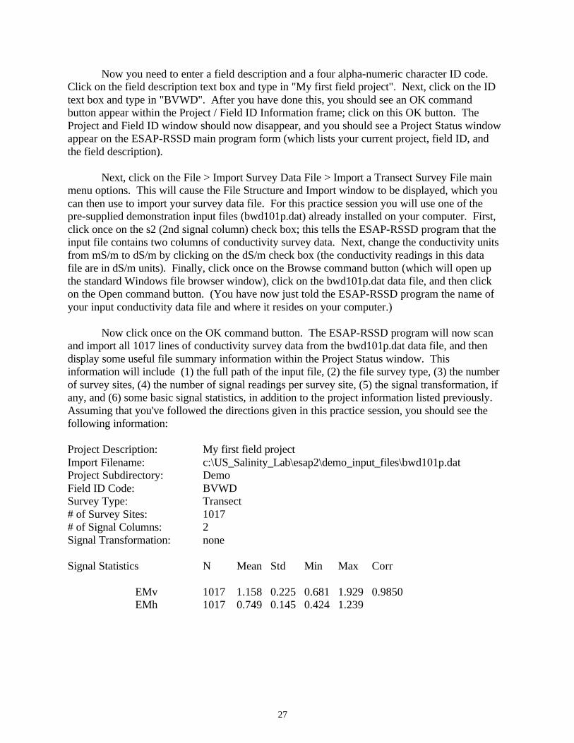
Now you need to enter a field description and a four alpha-numeric character ID code. Click on the field description text box and type in "My first field project". Next, click on the ID text box and type in "BVWD". After you have done this, you should see an OK command button appear within the Project / Field ID Information frame; click on this OK button. The Project and Field ID window should now disappear, and you should see a Project Status window appear on the ESAP-RSSD main program form (which lists your current project, field ID, and the field description). Next, click on the File > Import Survey Data File > Import a Transect Survey File main menu options. This will cause the File Structure and Import window to be displayed, which you can then use to import your survey data file. For this practice session you will use one of the pre-supplied demonstration input files (bwd101p.dat) already installed on your computer. First, click once on the s2 (2nd signal column) check box; this tells the ESAP-RSSD program that the input file contains two columns of conductivity survey data. Next, change the conductivity units from mS/m to dS/m by clicking on the dS/m check box (the conductivity readings in this data file are in dS/m units). Finally, click once on the Browse command button (which will open up the standard Windows file browser window), click on the bwd101p.dat data file, and then click on the Open command button. (You have now just told the ESAP-RSSD program the name of your input conductivity data file and where it resides on your computer.) Now click once on the OK command button. The ESAP-RSSD program will now scan and import all 1017 lines of conductivity survey data from the bwd101p.dat data file, and then display some useful file summary information within the Project Status window. This information will include (1) the full path of the input file, (2) the file survey type, (3) the number of survey sites, (4) the number of signal readings per survey site, (5) the signal transformation, if any, and (6) some basic signal statistics, in addition to the project information listed previously. Assuming that you've followed the directions given in this practice session, you should see the following information: Project Description: My first field project Import Filename: c:\US_Salinity_Lab\esap2\demo_input_files\bwd101p.dat Project Subdirectory: Demo Field ID Code: BVWD Survey Type: Transect # of Survey Sites: 1017 # of Signal Columns: 2 Signal Transformation: none Signal Statistics N Mean Std Min Max Corr EMv 1017 1.158 0.225 0.681 1.929 0.9850 EMh 1017 0.749 0.145 0.424 1.239

28

3.3 Data Visualization The graphics routines in ESAP-RSSD allow you to visualize your conductivity survey data using a number of different plotting techniques. These various plotting techniques are designed to help you better understand and interpret your survey data, and thereby assist you in the sampling design process. In general, you will create and view the majority of your graphs immediately after importing your conductivity survey data. However, some graphs can only be viewed after certain additional computations have been performed, and other graphs may contain additional visual information after performing such computations (as discussed below and in the on-line help documentation). 3.3.1 Description of Graphical Techniques There are six distinct types of graphs which the ESAP-RSSD program can produce, as described below. Survey Grid This plot will display the (x,y) location coordinates of your entire input data file, allowing you to verify that the survey data coordinates were correctly scanned into the ESAP program. Note that every survey grid is shown "true-to-scale"; i.e., ESAP does not distort or warp the (x,y) coordinates in any manner. The survey grid option is always active (i.e., enabled) whenever the ESAP Graphics Window is active. Therefor, you can produce a survey grid plot at any time. After you have performed a signal decorrelation on the input conductivity survey data (see section 3.4), any masked sites will be displayed as yellow points and any sites marked for deletion will be displayed as bright red points. (Once you delete a site, its location will no be displayed on the survey grid since this data will no longer be contained within the conductivity data file.) Additionally, any site selected as a sample site will be displayed as a light blue point on a survey grid plot. You can turn these color display options off from within the Graphics Initialization (GI) window. Scatter Plots Scatter plots provide you with an effective way to visualize the correlation structure between to variables. In ESAP, you may plot your s1 (1st column) or s2 (2nd column) survey data against either the x or y coordinate axis, or against each other (i.e., s1 versus s2). These plots will display the overall relationship between the above mentioned variables. The scatter plot options above are always active (i.e., enabled) whenever the ESAP Graphics Window is active. An additional scatter plot known as an "rsd plot" also becomes active after you have performed at least one signal decorrelation. RSD stands for "response surface design". When two input conductivity survey columns are present in your signal data file, this option will produce a plot of your 1st (z1) versus 2nd (z2) principal component scores.

29

When only one survey data column is available, this plot will display the values (i.e., magnitude) of the 1st principal component scores along the x axis (the y-axis values will simply contain small random perturbations, so that the 1-D principal component scores can be visualized in a 2-D plot). All masked sites and any sites marked for deletion will be clearly displayed on either type of rsd plot. In addition to the actual plots, some pertinent conductivity survey statistics will be displayed in the lower left hand side of the Graphics Window. These statistics will include the mean (u) and standard deviation (s) of whatever conductivity survey data is currently plotted, along with the calculated correlation (r) between the two variables currently displayed in the scatter plot. Note that by definition, principal component scores have 0 mean, unit variance, and are uncorrelated. Line Plots A line plot can be used to display the magnitude of the conductivity survey readings down an individual line (transect). These plots are most useful for detecting relationships between the bulk electrical conductivity and the transect coordinate position. For example, these types of plots can be used to check for the presence of tile lines (i.e., the plot will display a cyclic pattern) or head-to-tail salinity redistribution effects (the conductivity survey data will tend to increase in magnitude down the transect). The line plotting option is only available if you input a transect type conductivity survey file. Additionally, this option is disabled when the Graphics Window first activates; you need to enable (i.e., activate) it by opening up the GI window and initializing the line plotting option. When you initially request a line plot, ESAP will display a blank graph. On the left hand side of this graph you will see a frame bar titled "Line Plots" with the following command buttons: ">>", "<<", "Plot", "Refresh", "s1 Stats", "s2 Stats", and "Done". You can use the "Plot" button to create and display a line plot for any valid transect row number you request (the transect row number will be displayed immediately to the right of the Plot button). You can adjust the transect row number using the ">>" (up) and "<<" (down) buttons, and you can request that ESAP compute signal statistics for the current transect row number using the "s1 Stats" and/or "s2 Stats" buttons. If you wish to clear (i.e., erase) the current graph, you must use the "Refresh" button. Finally, when you are finished viewing the last line plot you should use the "Done" button to exit the line plotting mode. The statistics produced in the line plotting mode include the mean (u), standard deviation (s), and conductivity survey / transect coordinate correlation coefficient (r). However, note that the statistics calculated in the line plotting routines are based only on the currently displayed transect (rather than the entire survey data file). Also, if you display multiple conductivity transects on the same graph and then request any signal statistics, these statistics will only reflect the last transect shown on the graph.

30

Histograms A histogram represents a useful way to display the statistical distribution of a set of data values. In ESAP, you should use the histogram plots to examine the input conductivity survey data distributions. Typically, if the conductivity survey data is approximately Normally distributed then the conductivity histograms will appear approximately "bell-shaped". On the other hand, if the conductivity survey data is log-Normally distributed then the histograms will appear to be right-skewed, or if the signal data is bi-modal then the histogram will also appear bi-modal, etc. Histogram plots may sometimes also reveal data outliers, although this is not their primary purpose. In ESAP, the main purpose of the histogram plots is to help you determine if your input conductivity survey data should be log-transformed. The histogram option is disabled when the Graphics Window first activates; you need to enable (i.e., activate) it by opening up the GI window and initializing it. Also, when you request a histogram plot ESAP will also display some histogram statistics. These statistics include the mean (u), standard deviation (s), minimum (min), and maximum (max) of the requested variable. In addition to the s1, s2, z1, and z2 data, you may also produce a histogram of the calculated z1 transition standard deviations if a transition analysis has been perform on the decorrelated signal data (see section 3.4). This histogram (of the calculated transition standard deviations) can be used to indicate the overall distribution of short-range variability associated with your input conductivity survey data. ColorScale Grids A color-scale grid is simply an enhanced survey grid plot; e.g., a survey grid displayed using plotting symbol colors which correspond to the magnitude of the variable being plotted. If you are working with survey data collected on a dense, evenly spaced grid then you can use a color-scale plot to create a "quick-and-dirty" raster map of the spatial conductivity survey response pattern. If your input (x,y) survey coordinates are un-evenly spaced across the survey area or the survey grid is small (less than 500 sites), a color-scale grid tends to be less visually appealing. However, you can still generally ascertain the spatial survey response pattern, even under these latter conditions. The color-scale plotting option is disabled when the Graphics Window first activates; you need to enable (i.e., activate) it by opening up the GI window and initializing it. During the initialization process you can set the color-scale symbol plotting size and/or request a gray-scale grid rather than a color-scale grid. (This latter option is useful if you wish to print a color-scale grid plot out to a black-and-white printer.) When you request a color-scale grid ESAP will automatically display a legend button to the right of the graph. You can click on this button to display the color-scale legend (by default, ESAP displays all color or gray-scale grids using 3 program-determined cut-off values). In addition to the s1, s2, z1, and z2 data, you may produce a color-scale grid of the calculated z1 transition standard deviations if a transition analysis has been perform on the decorrelated survey data (see section 3.4). This color-scale grid (of the calculated transition

31

standard deviations) can be used to display the spatial distribution of short-range variability associated with your input conductivity survey data. Additionally, if you have already generated one or more soil sampling designs, then the locations of these sample sites can also be overlaid on any of the grids described above. Sample Site Maps Sample site maps can be produced from within the ESAP Graphics Window once one or more SRS sample designs have been generated (and/or a user defined sampling plan has been specified). Sample sites for each requested sampling design are automatically labeled on these maps (the labels are set equal to the site ID numbers). Typically, these maps are used by the sampling crew to navigate back to the soil sampling sites. Like a survey grid, all sample site maps are shown "true-to-scale". Additionally, this plotting option is automatically enabled once one or more sampling designs are generated by the ESAP program. 3.3.2 Navigating the ESAP-RSSD Graphics Menu Bar Graphics Menu Bar: Layout The ESAP Graphics menu bar is located in the upper left corner of the Graphics Window. The full layout for this menu bar system is shown below. Main level Sub-Level 2 Sub-Level 3 Graphics --> Survey Grid | --> Scatter Plots --> s1 vs x | --> s1 vs y | --> s2 vs x | --> s2 vs y | --> s1 vs s2 | --> rsd plot | --> Line Plots --> s1 by row | --> s2 by row | --> s1 and s2 by row | --> Histograms --> s1 | --> s2 | --> z1 | --> z2 | --> trans analysis |

32

--> ColorScale --> s1 | Grids --> s2 | --> z1 | --> z2 | --> trans analysis | --> overlay sample sites |

--> Sample Site Map

Options --> Initialize Graphic Components | --> Perform Coordinate Translation Print --> Print Current Graph Help --> OnLine Help --> Navigating the Graphics Menu --> Graph Descriptions / Information Exit --> Return to Main ESAP Program Menu Graphics Menu Bar: Menu Item Descriptions The main level contains 5 menu bar items; Graphics, Options, Print, Help, and Exit, which are self-explanatory. The sub-level menu items located beneath these 5 main options are defined as follows: ( from within Graphics ) Survey Grid This option can be used to produce a map of your survey grid (i.e., a plot of the survey coordinates). Scatter Plots This option can be used to produce scatter plots of the 1st (s1) or 2nd (s2) conductivity survey readings against the x or y coordinates, or against each other. This option can also be used to produce a response surface design (rsd) plot. Line Plots This option can be used to produce line (transect) plots, provided you imported a Transect type survey file. You can plot the 1st (s1) and/or 2nd (s2) conductivity survey readings against either the x or y row coordinates. Note that this line plotting option must be initialized before any line plots can be displayed.

33

Histograms This option can be used to produce histogram plots of the 1st (s1) or 2nd (s2) conductivity survey readings, or the primary (z1) or secondary (z2) decorrelated principal component scores. This option can also produce a histogram of the z1 transition standard deviation estimates (provided you imported a Transect type survey file and requested ESAP to perform a transition analysis). Note that this histogram plotting option must be initialized before any histogram plots can be displayed. ColorScale Grids This option can be used to produce color-scale grids, which are simply survey grid plots where the plotting symbol colors correspond to the magnitude of the data being plotted. ColorScale grids can be produced for the 1st (s1) or 2nd (s2) conductivity survey readings, the primary (z1) or secondary (z2) decorrelated principal component scores, and the z1 transition standard deviation estimates (again, assuming this data is available). If sample sites have been selected, then these sites can also be overlaid on the grid. Like the line and histogram plots, the color-scale plotting option must be initialized before any color-scale plots can be produced. Sample Site Map This option can be used to produce the final ESAP generated sample site maps for your survey data. Note that this option only becomes available after you have generated one or more sampling designs. ( from within Options ) Initialize Graphic Components This option should be used to open the Graphics Initialization window, which can in turn be used to initialize the line, histogram, and color-scale plotting routines discussed above. Perform Coordinate Translation This option can be used to open the Coordinate Translation window, which can in turn be used to adjust and/or rotate you (x,y) survey data coordinates. ( from within Print ) Print Current Graph Any graph produced within the graphics window can be printed using this option. Note that the print-out will simply be a screen dump of the entire graphics window.

34

( from within Help ) OnLine Help: Navigating the Graphics Menu This documentation explains how to use the Graphics menu bar, and describes the menu bar features. OnLine Help: Graph Descriptions / Information This is the help documentation you should read if you need help interpreting and/or understanding any of the graphs mentioned above. This documentation also contains some useful tips on when and how to best use each of the graphic procedures when running the ESAP-RSSD program. ( from within Exit ) Return to the Main Program Menu Select this option to close down the graphics window and return to the main program menu. 3.3.3 Invoking and Using the GI and CT Windows The Graphics Initialization (GI) window should be used to initialize all Line (Transect) plots, Histogram plots, and ColorScale grids. You can invoke and display the GI window by clicking on the Options > Initialize Graphic Components menu option. By default, the plots specified above are not initialized when the Interactive Graphics Window is first activated. Hence, their corresponding graphic initialization procedures must be specifically requested before you can view these plots. Both Histogram plots and ColorScale grids can be created from either a gird or transect survey data file. However, Line plots can only be created from a transect data file. Additionally, the transect direction (north-south or east-west) must be specified when requesting Line plots. The Graphics Initialization window can also be used to turn off one or both symbol highlighting options (i.e., highlight all masked and outlier sites, and highlight all selected sample sites). By default, both highlighting options are automatically turned on when the Interactive Graphics Window is first activated. Additionally, you can also change the ColorScale symbol plotting size and/or change the ColorScale grid to a GrayScale grid (provided you initialize the ColorScale grid graphing option). The Coordinate Translation window can be used to adjust the survey location (x,y) coordinates corresponding to the input conductivity survey data. You can invoke and display the

35

CT window by clicking on the Options > Perform Coordinate Translation menu option. However, you should be aware that all coordinate translation(s) are applied to the original (x,y) input data. Hence, any translation will remain in effect until it is removed by applying a reverse translation. Generally speaking, the only time you should invoke this window is (1) if either the x and/or y axis of your input coordinate system needs to be reversed (or swapped), or (2) you need to temporarily rotate the coordinate system in order to plot your transect survey lines along the north-south or east-west direction. In either case, the sample site selection algorithms in the ESAP-RSSD program will not be affected by any of the translation options available in this window. However, in the second scenario, you will need to apply a reverse translation in order to restore the original coordinate system. 3.3.4 Practice Module (Graphing Data) In this practice session you will learn how to use the ESAP-RSSD interactive graphics routines to display various features of your soil conductivity data. (Note: this practice session will make use of the previously imported bwd101p.dat survey data file. If you have not already done so, you should go back and complete practice module 3.2.3 before proceeding with this section.) From the ESAP-RSSD main menu screen, click on the Graph > Open Graphics Window menu options. This will cause the Interactive Survey Graphics (ISG) window to be displayed. Now click on Options > Initialize Graphics Components from within the ISG menu screen. This in turn will cause the Graphics Initialization window to be displayed. You can now use the options on this window to initialize the Line, Histogram, and ColorScale graphics options. To initialize the above options, click on the appropriate check boxes (a graphics option will be initialized when the check box becomes "checked" and the color of the option description changes from black to blue). For the Line plot, you should also click on the "North / South" transect option (this tells the ESAP-RSSD program to plot your conductivity transect lines against the y-axis coordinates). Next, click on the "change ColorScale to GrayScale" check box, and change the ColorScale symbol plotting size from 4 to 6. Finally, click on the "Initialize" command button to initialize these graphics options. At this point, if you click once on the Graphics menu option within the ISG menu screen, you will see that there are five types of graphical procedures now available for you to use. These five procedures are Survey Grid, Scatter Plots, Line Plots, Histograms, and ColorScale Grids, respectively. You should try using each of these procedures now, and explore the various options available in each graphical routine. As practice, you should try recreating figures 3.1 through 3.6 (shown on the following pages) using the directions listed below each figure. You may also wish to review section 3.3.1 again before proceeding, if you are unsure of how to interpret any of these graphical displays.

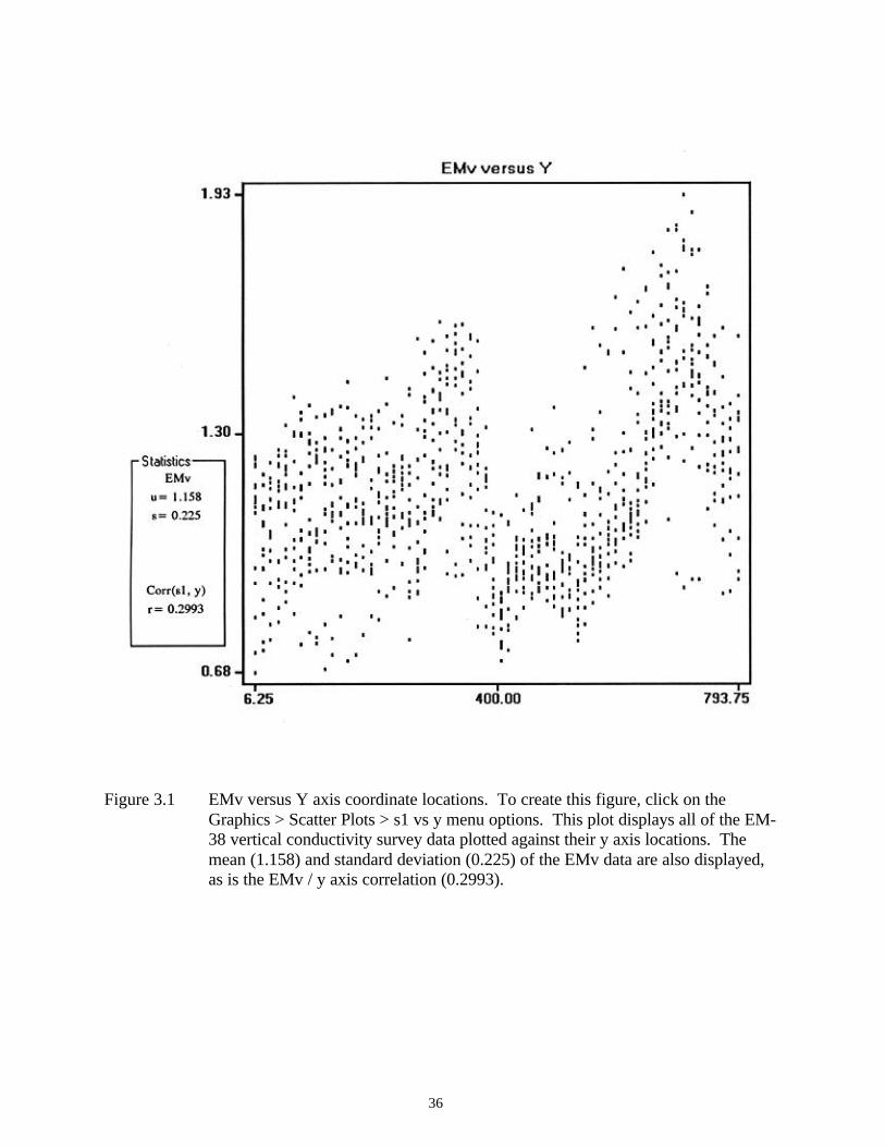
36

Figure 3.1 EMv versus Y axis coordinate locations. To create this figure, click on the

Graphics > Scatter Plots > s1 vs y menu options. This plot displays all of the EM-38 vertical conductivity survey data plotted against their y axis locations. The mean (1.158) and standard deviation (0.225) of the EMv data are also displayed, as is the EMv / y axis correlation (0.2993).

37

Figure 3.2 EMv versus EMh scatter plot. To create this figure, click on the Graphics >

Scatter Plots > s1 vs s2 menu options. This plot displays the correlation between the two conductivity survey readings (in this case, EMv versus EMh). Basic summary statistics are also computed and displayed within the Statistics frame to the left of the plot.

38

Figure 3.3 EMv & EMh versus Y axis for Row # 1. This figure shows a line transect plot,

which represents an individual transect of your soil conductivity survey data. To create this figure, first click on the Graphics > Line Plots > s1 and s2 by row menu options. This will cause the Line Plot frame to be displayed; the options within this frame can now be used to create line plots. Now click on the Plot button, then on the s1 Stats button, and finally on the s2 Stats button to create the graph and statistics.

39

Figure 3.4 EMv & EMh versus Y axis for Row #7. If the Line Plot frame is still displayed,

this figure can be created as follows. Click on the Refresh button (to clear the screen) and then use (i.e., repeatedly click on) the ">>" button to scroll up to transect number 7. Now click on the Plot button, then on the s1 Stats button, and finally on the s2 Stats button to create the graph and statistics.

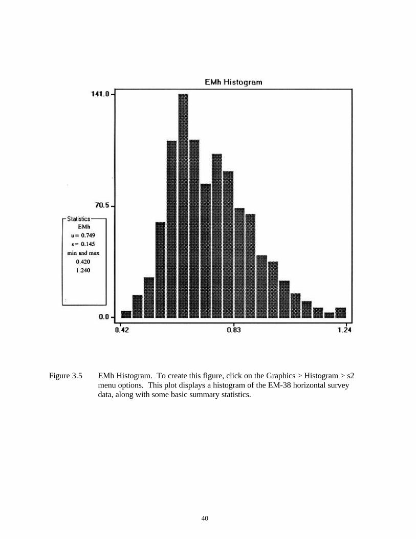
40

Figure 3.5 EMh Histogram. To create this figure, click on the Graphics > Histogram > s2

menu options. This plot displays a histogram of the EM-38 horizontal survey data, along with some basic summary statistics.

41

Figure 3.6 GrayScale Map of EMv Survey Data. To create this figure, click on the Graphics

> ColorScale Grids > s1 menu options. This plot displays a type shaded relief map, where the shades of gray represent different conductivity zones (4 zones from low to high).

42

Figures 3.1 through 3.6 represent only a portion of the plots that you can create in the ESAP-RSSD Interactive Graphics window. Hence, before leaving this practice module, we recommend that you try creating some additional plots using each of the five graphical procedures discussed above. 3.4 Data Analysis The following section describes how the ESAP-RSSD software program converts your conductivity survey data into transformed and decorrelated signal data, which is done primarily for the purpose of facilitating the generation of the sampling design(s). 3.4.1 Basic Statistics When the ESAP-RSSD program imports your conductivity survey data file, it automatically generates and displays a set of basic survey statistics on the main program frame. However, if desired, you can recompute these statistics using the options contained within the Signal Transformation / Scaling window. This window can be displayed by clicking on the Analysis > Basic Statistics main menu options. Normally, the only reason you would need to recompute these statistics is if you decide to shift or transform your raw survey data. The Signal Transformation Window allows you to either apply or remove a natural log transformation to/from your input conductivity survey data, and/or change the data units (mS/m <-> dS/m). However, note that this window can only be activated if you have not already invoked the Signal Decorrelation Option. There is a significant amount of contention within the soil salinity literature concerning the need (or lack there of) to log transform soil conductivity survey data. It has been our experience that most conductivity survey data sets need to be log transformed. We have seen some exceptions to this rule, especially if the soil salinity levels are very low (i.e., less than 1.0 to 2.0 dS/m). However, in general we recommend that you apply the log transformation if your ultimate objective is the prediction of the spatial soil salinity pattern. For other predictive purposes, whether or not you choose to log transform your input conductivity data will depend primarily on the statistical distribution of conductivity readings. You can generate histogram plots of your input data within the Interactive Graphics Window, and we recommend that you use these histogram plots to determine if your conductivity data need a log transform. If the histogram distribution(s) of your data appear to be approximately "bell-shaped", then you probably don't need to apply a log transformation. On the other hand, when the distributions are strongly "right-skewed" then a log transformation should definitely be applied. If the histograms do not clearly look either bell-shaped (Normal) or right-skewed (Lognormal), then you will need to base your decision on your own personal survey experience.

43

ESAP does not currently support any other type of transformation (or than the natural log). However, you are free to apply any type of transformation you wish to your survey data before it is imported into the ESAP-RSSD program. 3.4.2 Using the Iterative Decorrelation / Validation Algorithms The ESAP-RSSD program uses a statistical technique known as a response surface sampling design to select the final sample Sites. In order to facilitate this design, all conductivity survey data must first be centered, scaled, and decorrelated. (To completely understand how the signal decorrelation and validation routines facilitate the development of a response surface sampling design, you should refer to the research article by S.M. Lesch, D.J. Strauss, and J.D. Rhoades, 1995b.) This scaling and decorrelation process is carried out by the signal decorrelation routine. A by-product of this decorrelation analysis is that outlier (i.e., highly unusual) survey readings become very easy to detect. In ESAP-RSSD, detecting and removing outliers is referred to as signal data validation. In essence, the signal validation routines are simply "outlier removal" routines. To effectively use these routines, you just need to remember that the centered, scaled, and decorrelated survey (signal) data is measured in standard deviation units (std). For example, suppose you set the site outlier level (within the Signal Decorrelation window) to 5.0. Then what you are actually doing is telling ESAP-RSSD to identify all survey Sites with conductivity readings more than 5 standard deviations away from the mean (average) level of the survey data. In the ESAP-RSSD program, the default standard deviation levels for site masking and outlier detection are 3.5 and 4.5 std units, respectively. (For most survey applications these values should be adequate.) Invoking the Signal Decorrelation Algorithms In practice, you should use the signal decorrelation and validation routines in an iterative manner. First, you should open the Signal Decorrelation window by clicking on the Analysis > Signal Decorrelation main menu options. The decorrelation algorithm can be invoked; this will automatically scale and decorrelate your input conductivity survey data. If you have collected only one column of conductivity survey data, then the decorrelation algorithm will simply center and scale this survey data. If you have collected two columns or survey data (i.e., two conductivity readings per site), then the algorithm will perform a principal components decorrelation on this data in addition to the centering and scaling computations. Keep in mind that you must open this window to initiate the decorrelation algorithm, and this algorithm must be invoked before attempting to validate your decorrelated signal data. Invoking the Signal Validation Algorithms After your survey data has been decorrelated, your next step should usually be to open up the Signal Validation window by clicking on the Analysis > Signal Validation main menu options. The Signal Validation algorithm can be used to validate your decorrelated input conductivity survey data. If outlier survey data was detected during the decorrelation analysis,

44

then the validation algorithm will offer you two options. You can either (1) delete the outlier survey data Sites and then perform a new signal decorrelation, or (2) you can elect to mask these outlier Sites instead and end the validation process. If desired, you can also perform either an edge buffering or a transition analysis on your decorrelated survey data from this window (provided you are working on a Transect type input file). Handling Outlier Signal Data When one or more outlier survey data Sites are detected by the ESAP-RSSD program, the recommended approach is to delete the outlier Sites and perform a second decorrelation and validation iteration. Indeed, this is why the signal decorrelation and validation routines (and windows) have been designed the way they are. From a programming perspective, both the decorrelation and validation routines could actually be combined into a single process. However, these routines have been kept separate so that you can graphically analyze your decorrelated survey data -- before deleting any outliers. Thus, in most applications where outlier data Sites are detected, you should visually display your decorrelated survey data using one or more of the graphical displays available in the Interactive Graphics window. This in turn will allow you see both where the outliers are located (within the survey area) and how serious the outliers are (with respect to the rest of the survey data). 3.4.3 Additional Transect File Validation Options If you are processing a transect type signal data file, then two additional post-validation options will be available for use: (1) edge buffering, and (2) a transition analysis. The edge buffering option (which is located within the Signal Validation window) can be used to mask out all your survey Sites located within approximately 4% of the edges of your field (or survey area). This buffering technique is useful when you wish to keep your final sample site locations off the edges of the survey zone. Like edge buffering, a transition analysis can be performed on a transect type survey data file. A transition analysis quantifies the "short-scale" signal variability; i.e., this analysis identifies how different each conductivity survey reading is from its closest neighbors. This transition variability information can then be optionally incorporated into the SRS sampling algorithm in order to choose Sites with low variation. In practice, there is really only one situation when you might wish to incorporate transition variability information into the design; e.g., if you are using a low grade GPS unit to relocate the sample Sites. Low grade GPS units typically can not achieve sub-meter accuracy. Hence, when using such units you would naturally want to choose regions within your survey area which do not exhibit large conductivity variations over short distances. In such a scenario, a transition analysis may help you avoid degrading your calibration equation (i.e., prediction model) by minimizing the negative effects of any relocation errors.

45

You may also perform a transition analysis if you wish to visually detect any zones within your survey area having rapidly changing conductivity levels. (Transition variability information can be displayed graphically using the Interactive Graphics routines discussed earlier). If you perform a transition analysis solely for this purpose, you should make sure that you tell the ESAP-RSSD program not to use the transition variability information when generating any sampling designs (see section 3.5). Additional information about both the edge buffering and transition analysis options can be found within the on-line help documentation associated with the Signal Validation window. 3.4.4 Practice Module (Data Analysis) In this practice module you will learn how to perform an iterative signal decorrelation and validation analysis on your soil conductivity data. (Note: this practice session will make use of the previously imported bwd101p.dat survey data file. If you have not already done so, you should go back and complete practice modules 3.2.3 and 3.3.4 before proceeding with this section.) Recall from figure 3.5 that the EM-38 survey data appears to be log-Normally distributed. Hence, log transforming this data would be advantageous. To do this, click on the Analysis > Basic Statistics menu option. When the Signal Transformation window appears, highlight (i.e., check) the Apply Natural Log Transformation option and change the signal labels from "EMv" and "EMh" to "lnEMv" and "lnEMh". Now click on the Compute command button to apply the log transformation. At this point, you would normally go back into the Interactive Graphics window and view the new lnEMv and lnEMh histograms. (If you like, you can do this now. Note that the new histograms appear to be much more "bell-shaped"; i.e., the log transformed data now appears to be nearly Normally distributed.) Once you have finished producing any desired graphics, you should click on the Analysis > Signal Decorrelation menu option. This will invoke and display the Signal Decorrelation window. To invoke the decorrelation algorithm, click on the Perform Decorrelation command button. Note that the ESAP-RSSD program has found 5 Sites above the masking STD level (currently set to 3.5 standard deviations), and 2 of these Sites exceed 4.5 standard deviations (these are flagged as outlier Sites). Next, click on the List all Sites above Outlier STD level command button. You should now see the following information printed to the screen:

46

Site ID X-Coordinate Y-Coordinate Sig 1 Sig 2 STD 897 270.00 768.75 -0.119 -0.389 4.74 988 288.00 368.75 -0.224 -0.494 4.86 These are your two outlier Sites. To better determine where these Sites are located (within the survey area) and just how far removed from the rest of the survey data they are, open up and display the Interactive Graphics window. (To do this, first close out the Listing of Outlier Sites window, and click on the Finished command button in the Signal Decorrelation window. Then click on Graph > Open Graphics Window to display the IG window.) Now click on the Graphics > Survey Grid graph menu option. This should produce a grid map of the survey site locations, with the 2 outlier Sites colored red and the 3 other masked Sites colored yellow. Note that the 2 outlier Sites occur on the far right-hand side of the survey zone. Next, click on the Graphics > Scatter Plots > rsd plot graph menu option. This should reproduce the response surface design (rsd) plot shown in figure 3.7 below. Note that this plot clearly identifies how far removed the 2 outlier Sites are from the rest of the decorrelated survey data. Once you have finished viewing this plot, exit out of the IG window.

Figure 3.7 A rsd plot of the decorrelated bwd101p.dat EM-38 survey data.

47

Based on the rsd plot, it would probably be best to delete these two Sites and re-preform the signal decorrelation. To do this, click on the Analysis > Signal Validation menu option, make sure the delete all outliers... option is high-lighted, and then click on the Invoke Validation command button. This should cause the Signal Decorrelation window to be re-displayed. Now perform another decorrelation (by clicking on the Perform Decorrelation command button). Note that no further outliers are detected, although the 3 masked Sites are still present. At this point, you have now determined that your conductivity survey information contains no further outlier data Sites. Hence, click on the Finished command button in the Signal Decorrelation window, and then click on the Analysis > Signal Validation menu option to re-display the Signal Validation window. You should now see that the no outliers detected... option is high-lighted, implying that this data has been validated. Although it is not necessary for this data set, for practice you should go ahead and check the Invoke Edge Buffering Algorithm option, and make sure that the "mask all Sites in 1st and last rows" option is set to Yes. Now click on the Accept Configuration command button. You should then see the following two messages printed to the screen: Note: 217 Sites were masked by the edge buffering algorithm. Data file information saved to BVWDinfo.txt. These messages are telling you that 217 Sites around the edge of the survey zone have been masked (i.e., removed as potential sample site locations), and that all of the information currently displayed in the main ESAP-RSSD window has just been saved to a text file called BVWDinfo.txt. They also indicate that you have now finished your interactive signal decorrelation and validation analysis, and prepared your conductivity survey data for the ESAP spatial response surface (SRS) sampling design algorithm. 3.5 Generating Sampling Designs This section reviews the two ESAP-RSSD procedures for generating sampling designs, and describes when and how to use each procedure. 3.5.1 The Manual Sample Site Selection Procedure The manual sample site selection procedure can be used to manually create a custom (i.e., user specified) sampling design. This procedure should be used if you wish to specify your own set of sample Sites. To display the Manual Sample Site Selection window (which can be used to invoke this manual selection procedure), click on the Design > Manual Sample Site Selection menu option.

48

The ESAP-RSSD on-line help documentation states that there are normally just two scenarios where you would need to use this selection procedure. Actually, there are three possible scenarios where this procedure is useful, as described below. The first is to re-generate a design which was already created by the ESAP-RSSD program during an earlier sampling period. For example, suppose that you've already surveyed the field you are working in once before and used ESAP to generate the sampling design. You now re-survey this field (by collecting new survey data at all of the previously established survey grid Sites) and you'd like to acquire your soil samples at the same set of (earlier) sample Sites. Because the new survey data is different, ESAP would probably not choose the exact same set of Sites during the second sampling iteration. However, you can force the program to re-select the same set of Sites by creating a manual sampling design which exactly matches the first spatial response surface (SRS) design. Along the same line of reasoning, you may also need to re-generate a sampling design which has already been performed just so that you can use the ESAP-95 software programs (particularly ESAP-Calibrate and ESAP-SaltMapper) to analyze your data. As described above, you can force the program to select a specific set of Sites by creating a manual sampling design which matches the (already acquired) sample Sites. The second is for design comparison (research) purposes. For example, in your particular application it may be desirable to compare the efficiency of the design(s) created by ESAP to a more traditional sampling plan (such as a simple random sampling design, or stratified design, etc.). In these situations you can generate the more traditional design using some other software package, and then identify these Sites within ESAP using the manual sample site selection procedure. This technique can be used to insure that none of the ESAP generated SRS designs "overlap" with the traditional design (ESAP will not include any user specified sample Sites in any SRS generated designs). The third scenario (not discussed in the on-line help) is unusual, but very important. The ESAP-RSSD program is designed to create and output your *.svy data file automatically, once you are finished processing your survey data (recall that this is the processed survey data file used by the ESAP-Calibrate and ESAP-SaltMapper programs). However, this automatic *.svy file creation process can only occur if at least one sampling design has been first created and saved. In other words, you can not create the *.svy output data file unless you create a sampling design. This issue becomes important in the following situation. Suppose you intend to collect conductivity data only, and then use the deterministic calibration technique available in the ESAP-Calibrate program to convert this conductivity information into calculated salinity levels. Hence, you would not be collecting any soil sample data in this particular survey process, just conductivity information. However, to generate the *.svy data file (which the ESAP-Calibrate program needs), you must generate a sampling design. The solution here is to invoke the manual sample site selection procedure, select a single sample site (any site will do), and then save this sampling design. This will then "trick" the ESAP-RSSD program into generating the output

49

*.svy data file, thus creating an input file which the ESAP-Calibrate program can process. A few other points about the manual site selection procedure should be kept in mind. First, the Manual Sample Site Selection window can no longer be activated after you create and save one or more spatial response surface (SRS) sampling plans. So if you need to generate a manual design, you should do it first (before you generate any ESAP-RSSD SRS designs). And second, please note that ESAP uses the site-ID numbers to identify all manually selected sample Sites. Therefor, if you wish to use this procedure, you should include a site-ID column in your input conductivity survey data file and have access to these site-ID numbers in order to properly identify your set of sample Sites. 3.5.2 Generating ESAP-RSSD Spatial Response Surface (SRS) Sampling Designs The SRS Sample Site Selection window can be used to invoke the SRS (spatial response surface) sampling algorithm. This window can be displayed by clicking on the Design > Calculate SRS Sample Design menu option. You can then use the features contained within this window to select the sample design size, adjust some of the design characteristics, and/or save any sample design files to your current active project. Additionally, if you wish you can generate up to 5 separate SRS sampling designs. After you invoke the SRS algorithm, the ESAP-RSSD program will update you as the algorithm converges. During this process you will see a number called the "Opt Criteria" (or just "Opt Cri") printed to the screen (this is short for optimization criteria). This number represents a measurement of how uniform (i.e., evenly spread across the field) the sampling plan is. Uniform sampling plans generally achieve a value of 1.15 or less, highly non-uniform sampling plans typically have values of 1.75 or more. By design, the ESAP-RSSD program will try to achieve as uniform a sampling plan as possible. However, good uniformity is not always achievable (all SRS sampling designs are constrained by the initial response surface design levels, which take precedence over the uniformity criteria). In general, smaller survey sizes lend themselves to better optimization, and smaller sample sizes (i.e., n=12 as opposed to n=20) are easier to optimize. In most situations you can employ the optimization criteria value to judge the degree of uniformity in a generated SRS design, using the guidelines listed below (for square or rectangular survey areas): Opt Cri Value Uniformity < 1.15 excellent uniformity 1.15 - 1.30 reasonable uniformity 1.30 - 1.50 moderate clustering 1.50 - 1.75 serious clustering > 1.75 excessive clustering (an unacceptable design)

50

When possible, you should always try to select a design with an optimization criteria of 1.30 or less. When your survey area is non-rectangular, the above guidelines can not be directly applied. In general, highly non-rectangular survey areas will produce significantly higher optimization criteria values, and it will be necessary for you to adjust the above levels. As a rule of thumb, you can derive an approximate adjustment factor as follows. First, produce a printout of your survey zone, and then draw the smallest possible rectangle you can around this zone. Next, calculate the approximate amount of area covered by your survey zone within that rectangle, and then divide 100 by this value to produce the adjustment factor. Finally, multiply the above Opt Cri values by this factor to produce the new ranges. For example, if your survey zone was a circle, then this circle would cover 78.54% of the smallest rectangle (actually, a square) which could be drawn to completely enclose it. Thus, since 100/78.54 = 1.273, we would calculate that a design having excellent uniformity within this circular survey area should produce a value at or below about 1.46 (i.e., 1.273x1.15 = 1.464). Likewise, a design with excessive clustering would produce a value above 2.28, etc. Adjusting the Advanced Design Options In most situations you should not need to adjust the advanced design options. However, if your generated SRS design does not produce an optimization criteria value less than 1.30, then we recommend that you change the design factor and re-run the SRS algorithm. Try setting the design factor to values of 0.90, 0.95, 1.05, and/or 1.10, re-generate the sampling design, and see if any of these new designs produce optimization criteria values less than 1.30. Note that lowering the design factor shrinks the response surface design levels (resulting in a more conservative design). Likewise, raising the design factor causes the response surface design levels to expand (resulting in a more aggressive design). In general, we recommend that you try lowering the design factor first. If changing the design factor does not solve the site clustering problem (i.e., the Opt Cri value is still > 1.30) then you should invoke the parsing option. Data parsing can be employed on any conductivity survey data set with more than 400 survey Sites (data sets with only a few hundred observations rarely exhibit poor optimization criteria values). When you invoke the parsing option, ESAP will separate your survey data into 2 or more distinct strata (the number of strata ESAP uses will increase as your sample size increases). You should then select one of these strata to use (from within the Data Parsing / Stratification Window), invoke the SRS algorithm, and see if the Opt Cri value decreases. Note that you will need to repeat this process for every available strata, in order to determine which strata produces the lowest Opt Cri value (you should not save any of the generated SRS designs while you determining what their Opt Cri values are). Once you identify the best strata to use you should invoke the parse data option one last time, select that particular strata, generate the SRS sample design again, and then save it. The data parsing routine will often create more than one strata which can produce SRS Opt Cri design values below 1.30. Note that any of these strata can be used to produce your final design. Also, if none of the strata produce good designs, then try changing the design factor value by 0.1 units and repeating the process.

51

Additional Considerations If you have invoked the edge buffering option then the ESAP-RSSD program will not select any sample Sites from the edge buffered area, regardless of how you adjust any of the advanced design options. If you have invoked the transition analysis option, you also have the option of ignoring the TA information. You should be aware that sometimes a transition analysis will improve the optimization criteria, and sometimes this analysis will degrade it. However, in general we don't recommend employing and/or removing the TA information to improve the optimization criteria. Finally, keep in mind that you can generate up to 5 separate (i.e., non-overlapping) SRS sampling designs in the ESAP-RSSD program. However, unless you wish to generate either multi-stage or composite sampling plans, you probably will not need to use this feature. 3.5.3 Practice Module (Generating an SRS Sampling Design) In this practice module you will learn how to use the basic features of the SRS Sample Site Selection window to generate spatial response surface sampling plans. (As with all the previous practice modules, you will be using the bwd101p.dat conductivity survey data as your training data set. Therefor, in order to complete this module, you will need to have already performed practice modules 3.2.3, 3.3.4, and 3.4.4.) You can display the SRS Sample Site Selection window by clicking on the Design > Calculate SRS Sample Design main menu option. After this window first appears, you should first set the sample size. (In the ESAP-RSSD program the sample size will always default to n=12, and for this practice module you should leave it at this setting.) You should also note the Algorithm Status message (shown in green type); this message label will always display the current status of the sampling algorithm. To generate your design, click on the Invoke SRSS Algorithm command button. The ESAP-RSSD program will then display your survey grid, cycle through a series of algorithm iterations until an optimal design is determined, and then display the final optimization criteria value (Opt-Criteria) in the status message label. (This process may go by quite quickly if you are working on a fast computer.) In this example, the final Opt-Criteria value should be equal to 1.202. Since this is below 1.3, you can go ahead and save this design by clicking on the Save Current Design command button. After you have done this, you should see a message which says: SRSD sampling design information has been saved to BVWDrsd1.txt. This message is telling you that you have successfully saved your ESAP-RSSD generated SRS sampling design information to the above referenced text file.

52

That's all there is to it. However, for additional practice, you might at this point try generating one or two additional designs. Feel free to change the sample size setting (to either 6 or 20), and perhaps adjust the design factor. You might also try invoking the parsing option (especially if you want to generate a sampling design of size 6 which achieves an Opt-Criteria close to 1.3). 3.6 ESAP-RSSD Data Output This section describes how to view, print, and/or save the various output text files (and data plots) produced by the ESAP-RSSD program. 3.6.1 Text Output Unlike ESAP-Calibrate or ESAP-SaltMapper, the ESAP-RSSD program automatically creates and saves output text files relating to your analysis. If you have worked through the practice modules, you now probably realize that these files are automatically created at specific points throughout the operation of the program. For example, immediately after you completed the data validation step, the ESAP-RSSD program created and saved a text file called xxxxinfo.txt (where "xxxx" corresponds to your 4 character alpha-numeric field ID code). Likewise, the first time you saved an SRS sampling design, the ESAP-RSSD program created a text file called xxxxrsd1.txt. (If you saved a second SRS design, then ESAP-RSSD also created a text file called xxxxrsd2.txt.) Finally, if you had created and saved a manually generated sampling design, then ESAP-RSSD would have created a text file called xxxxugsd.txt ("ugsd" is an abbreviation for user generated sampling design). Any of the above mentioned files can be viewed or printed by clicking on the File > View / Print Output Files menu option. You can then highlight and open these text files using your default text editor (which will be WordPad, unless you have reset it to something else). If desired, you can save any or all of these files under different file names using the "save file as" feature in your text editor. The contents of each type of ESAP-RSSD output text file are summarized below: File Type Contents xxxxinfo.txt General data processing information, including all information displayed in the Project Status frame (except for any sample site design information). xxxxrsd#.txt SRS sample design information, including a list of the physical sample site locations and a summary of the SRS algorithm settings.

53

xxxxgps#.txt A sorted list of the sample site locations and ID numbers, produced along with each rsd#.txt output file (this text file can be used as input to a GPS data logger for automatically re-locating the sample Sites). xxxxugsd.txt User generated (i.e., manual) sample design information. 3.6.2 Graphical Output All graphs produced by the ESAP-RSSD program are created using the Interactive Graphics window. Additionally, any graph you create and display can also be printed using the Print > Print Current Graph menu options within this window. Unlike the SaltMapper and Calibrate programs, the ESAP-RSSD program does not currently allow you to save any graphs as bitmap files. 3.6.3 Creating an Output *.SVY Data File Creating the final output *.svy data file represents a critical step in your survey data analysis session; you must create this file if you wish to continue processing your survey data using either the ESAP-SaltMapper or ESAP-Calibrate programs. For this reason, the ESAP-RSSD program has been designed to automatically generate and save this file when you exit out of your analysis session. However, you MUST exit out of the program using the File > Exit main menu options. If you click instead on the upper right “X” (close program button) on the main RSSD window to exit the program, then your *.svy data file WILL NOT BE CREATED. Hence, you should NEVER exit the ESAP-RSSD program in this manner (by clicking on the close program button) unless you do not wish to create an output *.svy data file. Note also that unless you have generated and saved at least on sampling design (either an SRS or user generated sample design), the ESAP-RSSD program will NOT generate an output *.svy data file. 3.6.4 Practice Module (Viewing and Printing Output Data) This is the final practice module for Chapter 3. If you have performed all of the previous modules, you should be able to re-create the output data shown on the next few pages. In most survey situations there will be three items (files or graphs) that you should always make hard copy prints of: (1) your sample site map, (2) your rsd sample site documentation information file, and (3) your general information log file. To produce a plot of the sample site locations generated in practice module 3.5.3, invoke and display the Interactive Graphics window. Next, click on the Graphics > Sample Site Map graph menu option to display the Sample Site Labeling window. High-light the RSD sample Sites from Design #1 check box

54

option, and then click on the Create Map command button. This should produce a map like the one shown in figure 3.8 below. Now click on the Print > Print Current Graph menu option to print a copy of this map, and then exit out of the Interactive Graphics window.

Figure 3.8 Response surface sampling design map for Design #1. To print out copies of the BVWDrsd1.txt and BVWDinfo.txt text files, click on the File > View / Print Output Files main menu option. This should cause the Windows File View window to be displayed; now simply high-light and open the desired file. Which ever file you select will then be displayed in WordPad (or what ever default text editor you are currently using). You should then be able to print out copies of these text files using your text editor menu options, etc. If you have followed the instructions given in each of the preceding practice modules, the hard copy of your BVWDinfo.txt text file should match the information shown in table 3.1. Likewise, your BVWDrsd1.txt text file should match the information shown in table 3.2.

55

The final step you still need to perform is to create the BVWDdata.svy processed conductivity survey file. To do this, simply click on the File > Exit main menu option. The Data File Export window should then appear, and 1015 lines of conductivity data should automatically be exported to this file. You can now safely exit the program by clicking on the Yes command button (contained within the Confirm Program Exit frame). Congratulations! You have just finished processing your first conductivity survey data file using the ESAP-RSSD software program.

56

Table 3.1 Hard copy print out of the BVWDinfo.txt text file _____________________________________________________________________________ Input File: C:\US_Salinity_Lab\esap2\demo_input_files\bwd101p.dat Output File: C:\US_Salinity_Lab\esap2\data\Demo\BVWDinfo.txt Project: Demo O-File Name: BVWDinfo.txt Date & Time: 11/29/1999 10:20:04 AM Field Desc: My first field project FieldID Code: BVWD File Type: Transect (rowcount = 16) Survey Size: 1015 # of Signals: 2 Signal Units: dS/m Sig Trnsfrm: natural log Signal Statistics lnEMv lnEMh N 1015 1015 Mean 0.129 -0.306 Std 0.191 0.190 Min -0.385 -0.858 Max 0.657 0.214 Signal Corr = 0.9839 Decorrelation Statistics Level # Sites > Level Masking STD 3.50 3 Outlier STD 4.50 0 Total # of deleted Sites: 2 # of Validation iterations: 1 Edge Buffering: invoked Transition Analysis: none

_____________________________________________________________________________

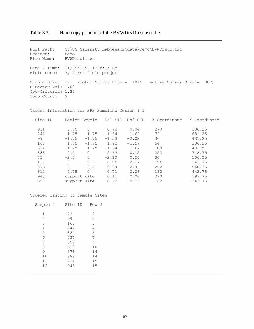
57

Table 3.2 Hard copy print out of the BVWDrsd1.txt text file. _____________________________________________________________________________ Full Path: C:\US_Salinity_Lab\esap2\data\Demo\BVWDrsd1.txt Project: Demo File Name: BVWDrsd1.txt Date & Time: 11/29/1999 1:28:15 PM Field Desc: My first field project Sample Size: 12 (Total Survey Size = 1015 Active Survey Size = 807) D-Factor Val: 1.00 Opt-Criteria: 1.20 Loop Count: 9 Target Information for SRS Sampling Design # 1 Site ID Design Levels Ds1-STD Ds2-STD X-Coordinate Y-Coordinate 934 0.75 0 0.73 -0.04 270 306.25 247 1.75 1.75 1.64 1.62 72 681.25 99 -1.75 -1.75 -1.53 -2.03 36 431.25 168 1.75 -1.75 1.92 -1.57 54 306.25 324 -1.75 1.75 -1.34 1.67 108 43.75 888 2.5 0 2.63 0.12 252 718.75 73 -2.5 0 -2.19 0.56 36 106.25 437 0 2.5 0.28 2.17 126 143.75 876 0 -2.5 0.34 -2.46 252 568.75 612 -0.75 0 -0.71 -0.06 180 443.75 943 support site 0.11 0.06 270 193.75 557 support site 0.22 -0.12 162 243.75 Ordered Listing of Sample Sites Sample # Site ID Row # 1 73 2 2 99 2 3 168 3 4 247 4 5 324 6 6 437 7 7 557 9 8 612 10 9 876 14 10 888 14 11 934 15 12 943 15

______________________________________________________________________________

58

[ this page intentionally left blank ]

59

4.0 ESAP-SaltMapper Software Program 4.1 ESAP-SaltMapper Program Overview The following section gives an overview of the ESAP-SaltMapper software program, including a review of how the program functions and a description of the main menu bar layout. 4.1.1 Program Description What is ESAP-SaltMapper ESAP-SaltMapper is a graphics program which can be used to generate, display and plot high quality 1-D transect graphs and 2-D raster maps of either your observed soil conductivity data or predicted soil salinity (or secondary soil variable) data. The ESAP-SaltMapper program is part of the ESAP software package for Windows; a multi-program software package designed and distributed by the United States Salinity Laboratory for the sampling, assessment, and prediction of soil salinity (and/or other soil variables) from electrical conductivity survey data. The ESAP-SaltMapper program is designed to read in (i.e., import) the output data files produced by the ESAP-RSSD and ESAP-Calibrate programs (*.svy or *.prd files, respectively). ESAP-SaltMapper preserves the structure of the survey or prediction file; i.e., it can recognize the difference between a transect and grid file and process either file type accordingly. Both 1-D transect graphs and 2-D raster maps can be created when transect files are imported into the ESAP-SaltMapper program. When grid files are imported, only 2-D raster maps can be created. In addition to its graphical capabilities, the ESAP-SaltMapper program can be used to create new data columns from the input data, and/or export any input data as a generic ASCII text file. The data creation feature is especially useful when you wish to combine or average 2 or more existing columns of survey or prediction data. Likewise, the export feature can be used whenever you wish to employ another graphing or database program to read or process any ESAP output data file. How does the ESAP-SaltMapper Program Work To create any type of graphical output using the ESAP-SaltMapper program, you simply need to import the survey (*.svy) or prediction (*.prd) data file you wish to process. Once you have successfully imported your data, you can create new data columns, produce graphics, and/or export your input data out to an ASCII text file. Please note that the ESAP-SaltMapper program has only been designed to process either ESAP-RSSD output survey data or ESAP-Calibrate output prediction data (i.e., *.svy or *.prd data files). At present, these are the only two file types that the ESAP-SaltMapper program can operate on.

60

4.1.2 Navigating the ESAP-SaltMapper Main Menu Bar Main Menu Bar: Layout The ESAP-SaltMapper Main menu bar is located in the upper left corner of the main program Window. The full layout for this menu bar system is shown below. Main level Sub-Level 2 Sub-Level 3 File --> Specify Project / Input File Info | --> Column Manipulation | | | --> Change Column Labels | --> Create a New Column | --> Column Statistics | | --> Create Output Data File | --> Exit Graphics --> 1D Line Transect Plot | --> 2D Raster Image Map Help --> About ESAP-SaltMapper | --> ESAP Interface Controls | | | --> ReSet default Text Editor | --> OnLine Help --> What is ESAP-SaltMapper --> Navigating the Main Menu --> Frequently Asked Questions (FAQ) Main Menu Bar: Menu Item Descriptions The main level contains 3 menu bar items; File, Graphics, and Help. You should use the File menu to access all the data input/output and column manipulation routines, the Graphics menu item to access either the 1D transect plotting routines or 2D raster mapping routines, and the Help menu to access the main ESAP program help files. Additional help file documentation is available for nearly all ESAP program routines; this documentation can be accessed by double clicking on the OnLine Help file button within whatever window is currently activated (the OnLine Help button is the small button displaying a capital "H", usually located in the lower right hand corner of the window).

61

Brief descriptions of the sub-level menu items (located beneath the 3 main program menu bar items) are given below: ( from within File ) Specify Project / Input File Info Select this menu option to open up the Project and Input File window, which is where you can set the current project and identify the input file. Note that you must define the input file type (either a *.svy or *.prd file) before you can import your data. Column Manipulation Select this menu option to manipulate one or more data columns. Your column manipulation choices include (1) changing one or more column labels, (2) creating one or more new data columns from a combination of existing data columns, and (3) computing the univariate column statistics, respectively. Create Output Data File Select this menu option to open up the ASCII File Export window, which can then be used for data export purposes. Exit Select this menu option to exit the ESAP-SaltMapper program. ( from within Graphics ) 1D Line Transect Plot Select this menu option to open up the 1D Line Plot window. This window contains the routines you will use to create and output various types of 1D line transect plots of your survey or prediction data. 2D Raster Image Map Select this menu option to open up the Raster Map Initialization window. From within this window you can then access the routines needed to create 2-D raster maps of your input survey or prediction data. Note that the raster map interpolation routines allow you to control the smoothness of your final map, as well as the mapping boundaries.

62

( from within Help ) About ESAP-SaltMapper Select this option to display the ESAP-95 Software information window. ESAP Interface Controls: ReSet default Text Editor You may use this option to change the default text editor used by ESAP-95 to display and print all ESAP generated help files. At program start-up, the default text editor package is set to "c:\windows\write.exe". OnLine Help: What is ESAP-SaltMapper Select this option to display the introductory help documentation. This is the help documentation you should read first if you have never used the ESAP-SaltMapper program before. This documentation explains what the ESAP-SaltMapper program does and how the program works. OnLine Help: Navigating the Main Menu This documentation explains how to use the Main menu bar, and describes the menu bar features. OnLine Help: Frequently Asked Questions (FAQ) This is the help documentation you should read if need more detailed information about how to use the various program features. For example, refer to this documentation if you don't understand the difference between a *.svy and *.prd file, or you wish to understand how a 2-D raster image is created, etc. 4.2 Data Input and Manipulation The following section describes how to import ESAP-RSSD (*.svy) or ESAP-Calibrate (*.prd) generated data files into the ESAP-SaltMapper program, and how to manipulate this data once it has been imported. 4.2.1 Setting the Current Project and Importing Data You should use the Project and Input File window to import your *.svy or *.prd data file into the ESAP-SaltMapper program. This window can be displayed by clicking on the File > Specify Project / Input File Info main program menu options. In order to successfully import your data file, you must perform the following three steps.

63

First, you must set the current project; i.e., you must identify which project your data file resides in. This can be done by clicking on the appropriate project name listed in the Set Current Project list box. Second, you must specify your data file type (either *.svy or *.prd) using one of the appropriate Input File type option buttons. Finally, you must specify the path and filename of your input file. This can be done by typing in the appropriate information into the Path / Filename input text box, or by using the Browse button to locate your input file. If you wish, you can also request that any natural log transformed data columns be back-transformed (using the check box option under Data Scale). If you request this option and your data has not been log transformed, then this request will be ignored. Please note that the ESAP-SaltMapper program is only designed to read in ESAP-RSSD generated *.svy or ESAP-Calibrate generated *.prd data files. If you attempt to import any other type of data file, then the ESAP-SaltMapper program will display an error message and halt the data file import process. 4.2.2 Renaming Columns Once you have imported a data file, you may change or rename any existing column labels. To display the Rename Columns window, click on the File > Column Manipulation > Change Column Labels menu options. You can then use the options within this window to change the current column labels. Note that if you requested that all log transformed data columns be back-transformed during the data import process, you will probably need to change your column labels (i.e., to remove any “ln” or “log” prefixes). 4.2.3 Creating New Data Columns In addition to changing column labels, the ESAP-SaltMapper program also gives you the capacity to create one or more new data columns from two or more existing columns of data. To create a new data column, you need to invoke and display the Create Data Column window. This window can be displayed by clicking on the File > Column Manipulation > Create a New Column menu options. Any new data column you create must be generated from a combination of existing data columns already present in your data file. Two types of data columns can be created by the ESAP-SaltMapper program, a new "ratio" column or a new "linear" column. A new ratio column is created from a ratio of two or more existing data columns; a new linear column is created from a linear combination of two or more existing data columns. In order to create either type of data column, you must define a set of appropriate summation weights. The example given below describes how to define appropriate summation weights for a typical modeling application. Assume for the moment that you have imported a *.prd data file which contains salinity

64

predictions across 4 sampling depths; i.e., you have 4 existing data columns labeled ECe(1), ECe(2), ECe(3), and ECe(4). Suppose further that you wish to create one new linear data column and one new ratio data column defined as follows: New linear column: (an average of the existing salinity columns) ECe(ave) = 0.25*ECe(1) + 0.25*ECe(2) + 0.25*ECe(3) + 0.25*ECe(4) New ratio column: (a salinity profile shape column) ECe(shape) = [ ECe(1) + ECe(2) ] / [ ECe(1) + ECe(2) + ECe(3) + ECe(4) ] To create the ECe(ave) column, you would select the Linear Estimates option under the New Column Type and then enter the following summation weights: Label Weights ECe(1) 0.25 ECe(2) 0.25 ECe(3) 0.25 ECe(4) 0.25 Likewise, to create the ECe(shape) column, you would select the Ratio Estimates option and then enter the following numerator and denominator weights: Label Weights Weights ECe(1) 1 1 ECe(2) 1 1 ECe(3) 0 1 ECe(4) 0 1 Note that in both cases the summation weights simply reflect the appropriate algebraic multiplication factors which would be used to recreate the mathematical formulas shown above. In general, the easiest way to define your specific summation weights is by writing out the mathematical formula for the new data column you wish to create, and then reading off the weights directly from this equation. After you have defined an appropriate set of summation weights, you should enter a label for your new data column in the new column label text box. This can be any descriptive label which is 14 characters or less in length.

65

4.2.4 Displaying Basic Column Statistics You can display basic summary statistics associated with each imported or created data column by clicking on the File > Column Manipulation > Column Statistics menu options. The displayed statistics will include the minimum, maximum, mean, and standard deviation for each column of data. Among other things, this feature is useful for determining the range and variability of newly created data columns. 4.2.5 Practice Module (Importing and Manipulating Data) All the practice modules contained within Chapter 4 (including this module) will make use of the BVWDdata.svy processed conductivity survey data file that was created during the last Chapter 3 practice session. Hence, if you have not already done so, you will need to complete the Chapter 3 practice modules in order to continue on with this session. In this practice session you will learn how to import data into the ESAP-SaltMapper program. You will also learn how to change some the imported column labels, and how to create and label a new data column. If necessary, start up the main ESAP-95 splash screen by clicking on the ESAP-95 prompt listed within the Programs drop-down menu system (i.e., click on Start > Programs > ESAP-95). Once the splash screen has displayed, click once on the ESAP-SaltMapper command button to invoke the SaltMapper program. After the ESAP-SaltMapper main menu screen is fully displayed, click on the File > Specify Project / Input File Info menu option. This will cause the Project & Input File window to be displayed. Make the Demo project your current project by clicking once on the Demo Project directory listed in the Set Current Project frame. Next, highlight the ESAP-RSSD input file option (you will be importing a *.svy data file), and then check the back-transform all log transformed data check-box (this tells the ESAP-SaltMapper program to back transform the log transformed EM signal data columns). Finally, click on the Browse command button, open the BVWDdata.svy data file, and click once on the OK command button. You should now see 1015 lines of processed conductivity data imported into the ESAP-SaltMapper program. Once the data has been imported, the ESAP-SaltMapper program should print the following message to the screen:

Note: don't forget to change the names (i.e., labels) of any columns associated with log transformed signal or prediction data.

This message is reminding you that any "ln" (or “log”) prefixes should be removed from the imported signal column labels. To do this, close down the displayed ESAP-SaltMapper message by clicking on the OK button. Next, click on the File > Column Manipulation > Change Column Labels main menu option; this will invoke and display the Rename Columns window. Now change the "lnEMv" and "lnEMh" labels to "EMv" and "EMh", and then click on the change

66

button. Note that the new column labels are immediately re-displayed in the Column Labels frame on the main SaltMapper window. You have now successfully imported your BVWDdata.svy data file and changed the EM column labels (to reflect the fact that these columns were back-transformed). Now it is time to create a new data column. For practice, you should create a new column of EM ratio data defined as EMratio = EMh / [ EMh+EMv ]. To create this new column, click on the File > Column Manipulation > Create a New Column main menu option. After the Create New Data Column window is displayed, highlight the ratio-estimates option and enter the following numbers into the weight text boxes: Column Labels: Weights: Weights: EMv 0 1 EMh 1 1 1st-PCS 0 0 2nd-PCS 0 0 Now type in "EM-ratio" in the New Column Label text box and click on the Apply command button. You should see a new column called EM-ratio appear in the Column Label frame on the main program window. If you like, you can view the statistics associated with this new data column by clicking on the File > Column Manipulation > Column Statistics main menu option. If you have created your new EM-ratio data column as instructed above, then these data should range between 0.371 to 0.421 and have a mean and standard deviation of 0.393 and 0.008, respectively. 4.3 Creating 1D Line (Transect) Plots The following section describes how to initialize, display, modify, and print a 1D line (transect) plot. 4.3.1 Definition of a 1D Line Plot A 1D line plot is simply a graph of your conductivity or prediction data down a specific transect, or survey pass. This type of plot can be used to display your data on a transect by transect basic, or data associated with multiple transects can be overlaid onto a single graph. 1D line plots can be created from within the 1D Line Plot window, which can be invoked by clicking on the Graphics > 1D Line Transect Plot menu option. In the ESAP-SaltMapper program, you can overlay up to 4 lines of data within a single plot. These lines can either be data arising from up to 4 different transects, or from 4 different variables associated with the same transect. For example, suppose you have imported an ESAP-Calibrate prediction data file that contains 4 columns of predicted salinity data (i.e., predicted

67

salinity data at 4 sampling depths). You could then create a 1D line plot which overlays the predicted salinity data within the first sampling depth for 4 different transect lines. Or you could overlay all 4 prediction depths for any given transect line, etc. If you wanted to, you could even mix the above two plotting styles (i.e., two lines with two variables displayed for each line). 1D line plots are most useful for detecting non-random data structure down survey passes. For example, such plots are commonly used to search for evidence of increasing head-to-tail conductivity trends (in flood or furrow irrigated fields) and / or cyclic patterns (which can indicate the effectiveness of any tile lines). Such plots can also sometimes be used to detect abrupt changes in soil texture (under non-saline conditions). 4.3.2 Navigating the 1D Line Plot Menu Bar 1D Line Plot Menu Bar: Layout The 1D Line Plot menu bar is located in the upper left corner of the 1D Line Plot program window. The full layout for this menu bar system is shown below. Main level Sub-Level 2 Plot --> Specify New Plot Variables | --> Create Plot Output --> Print | --> Save as Bitmap Help --> Navigating the 1D Line Plot Menu | --> 1D Line Plotting Tips Exit --> Return to Main Menu 1D Line Plot Menu Bar: Menu Item Descriptions The 1D line plot menu contains 4 menu bar items; Plot, Output, Help, and Exit. You can use the Plot menu to initialize the 1D line plotting options (Specify New Plot Variables) and display the initialized plot (Create Plot). You can use the Output menu if you wish to print the currently displayed line plot and/or save this plot as a bitmap file. Likewise, you should use the Help menu if you wish to access any 1D line plot help files. Brief descriptions of the sub-level menu items (located beneath the 4 main program menu bar items) are given below:

68

( from within Plot ) Specify New Plot Variables Select this menu option to open up the 1D Line Plot Initialization window. You will use the controls within this window to initialize each line plot you wish to create. Create Plot Select this menu option to create and display your 1D line plot. ( from within Output ) Print Select this menu option to print the currently displayed line plot. Save as Bitmap Select this menu option to open up the File Save window. You can then use this window to specify the path and name of your bitmap file, and then save this file. ( from within Help ) Navigating the 1D Line Plot Menu Select this option to display the Navigating the 1D Line Plot Menu help file. 1D Line Plotting Tips Select this option to display the Line Plotting Tips help file. This help file describes how you can add figure titles, labels, and/or a figure legend to your 1D line plot. ( from within Exit ) Return to Main Menu Select this option to close down the 1D Line Plot Display window and return to the ESAP-SaltMapper main menu. 4.3.3 Line Plot Initializing Options You should use the 1D Line Plot Initialization window to identify the specific transects (i.e., rows) you wish to display in your 1D line plot. This window can be displayed by clicking

69

on the Plot > Specify New Plot Variables line plot menu option. You can specify up to 4 transects per plot, and the data from each transect can represent different signal or prediction variables. Before a line plot can be created, you must specify which set of axis coordinates to plot the data by (i.e., either the x-axis or y-axis coordinates). You will also need to select the variables and rows you wish to plot. Additionally, you can set the line and symbol plotting styles for each line plot you create, as described below. (1) If you plot 2 or more lines of data, you can choose to display the lines using either the same

color of different colors. (2) If you plot 2 or more lines of data, you can choose to display the lines using either the same

line style (solid) or different line styles. (3) You can choose to show or hide the symbols on each line of data you plot. (Note: each

symbol shown represents a unique data point along the line.) (4) If you plot 2 or more lines of data and choose to display the data point symbols, you can

specify whether the symbols should be the same or different across the different lines. Once you have initialized all of the various options, you should click once on the Initialize button to initialize the 1D line plot. (Note: initializing the plot does not cause the plot to be displayed -- to display the plot you should click on the Plot > Create Plot line plot menu option.) 4.3.4 Adding a Title, Axis Labels, and / or Legend to a Transect Plot After you have displayed your line plot, you can refine the visual appearance of this plot by adding titles and labels and/or a figure legend. Beneath the displayed plot there will be a frame called Title and Labels. Inside this frame is an input text box, a "Figure Title" button, a "Plot Title" button, a "X-Label" button, and a "Y-Label" button. You can type a unique text string in the text box and then use any of these buttons to assign this text string into the appropriate title or label slot on the graph. (Note: adding a plot tile, x-label, or y-label will cause the displayed line plots to shrink slightly in size.) You can also display a legend in the upper right hand corner of the plot by clicking once on the Show button inside the Legend frame. After you click on the Show button, the button caption will change to Hide; simply click on this button again if you wish to remove (i.e., hide) the displayed legend. (Note: adding a legend to your graph will cause the displayed line plots to shrink in size.)

70

4.3.5 Practice Module (Creating a 1D Transect Plot) In this practice session you will learn how to create, display, and modify a 1D transect plot. To invoke and display the 1D Line Plot Display window, click on the Graphics > 1D Line (Transect) Plot main menu option. After this window appears, click on the Plot > Specify New Plot Variables line plot menu option. This will invoke and display the Line Plot Initialization window, which you can then use to initialize your 1D line plotting options. The first thing you must always do is specify which axis to plot your data by; this can be done by highlighting either the X or Y-coordinate location option in the X-Axis Variable frame. Then you should specify the data you wish to plot. This is done by using the different drop down Variable list boxes, selecting the variable to plot, and then specifying the corresponding transect row number. Finally, you can use the options contained within the Line Color, Line Style, Show Symbols, and Symbol Style frames to customize the look of the plot. For this practice module, highlight the Y-coordinate location option. Next, click on the first Variable list box and select "EMv", then click on the second Variable list box and select "EMh". Now click once on each [>>] command button (to the right of the Variable list boxes); this should increment the Row # values up to 2 in each row number text box. Finally, highlight the "Same style for each line" option in the Line Style frame, and then click on the Initialize Plot command button. After the Line Plot Display window disappears, click on the Plot > Create Graph line plot menu option. A 1D line plot of the EMv and EMh signal data down the 2nd transect should now appear. Next, locate the text box contained within the Titles and Labels frame, type in "Transect #2" (without the quotes), and click once on the Plot Title command button. Your plot should now have a title located in the upper left-hand corner that says "Transect #2". Next, type in "Distance down furrow (meters)" in the text box and click on the X-Label command button. Then type in "EM-38 (dS/m)" and click on the Y-Label button. You have now just added your X and Y axis labels, and your displayed plot should look like the plot shown in Figure 4.1. For additional practice, you may now wish to experiment with the 1D transect plotting features some more on your own. Feel free to modify the look of your plot, and/or create one or more new transect plots of different line data. Keep in mind that you can plot up to 4 rows of data on the same plot, and that each row can represent a unique variable and transect pass. You should also be able to print any transect plots you create using the Options > Print line plot menu option.

71

Figure 4.1 1D transect plot created in practice module 4.3.5. 4.4 Creating 2D Raster Maps The following section describes how to initialize, create, display, and print a 2D raster map. 4.4.1 About the Raster Map Creation Process The ESAP-SaltMapper program has been designed to allow you to generate 2D raster images of your survey or prediction data quickly and easily. However, in order to use this program feature effectively, you need to understand how the raster map creation process works. ESAP generates all rater maps (images) through a two stage process. The actual data interpolation is performed in the first stage, by using the on-screen interpolation controls in a systematic, sequential manner. Once the data interpolation is complete, raster maps of any survey or prediction variable in the current data set can be quickly created from the Raster Map menu commands. These menu driven, map creation commands represent the second stage of the image generation process. The remainder of this section describes the above mentioned two stage process in detail. We recommend that you read the rest of this section and try completing the practice module (4.4.5) before you attempt to generate any 2D raster images.

72

4.4.2 Using the Raster Map On-Screen Interpolation Controls To invoke and display the Raster Map Initialization window, click on the Graphics > 2D Raster Image Map main menu option. Once this window displays, you can begin the data interpolation process using the on-screen interpolation controls (i.e., the command buttons contained on the left hand side of the Initialization window). To interpolate your survey or prediction data, you should sequentially perform the following 6 steps described below. Step 1: Initialize Raster Window Click on this button to initialize the raster interpolation window. This will initialize (i.e., reset) the interpolation memory array and clear the interpolation window. Step 2: Show I-Grid / Survey Sites Click on this button to display the interpolation grid and plot the survey or prediction site locations within the raster interpolation window. Step 3a: Clip Grid (optional) Click on this button if you wish to clip away any sections from the interpolation grid, else proceed directly to either step 3b or step 4. From time to time you may acquire survey data which does not originate from a rectangular field. In these situations you may need to "clip" (i.e., remove) one or more sections of the interpolation grid so that the ESAP-SaltMapper program does not attempt to interpolate predictions into these non-surveyed areas. If you wish to initiate the clipping feature, you can do so as follows. After clicking on the "Clip Grid" button, move the mouse to the upper left corner of the area you wish to remove from the interpolation grid and click the left mouse button once. This initiates the clipping process. Now, move the mouse to the lower right corner of the area to be clipped. As you move the mouse you should see an expanding box appear on the screen; the interior of this box represents the area you can clip. Once you have enlarged the box to cover the area you wish to remove, you should click the left mouse button a second time. This second click defines the lower right corner of the box, and hence the area to be removed. After doing this you will see that section of the interpolation grid disappear and the background color of the clipped area change from white to yellow. This visually identifies this area as "clipped", and SaltMapper will avoid calculating any interpolated predictions within this region. Please note that in this current version of the ESAP-SaltMapper program you can only clip out rectangular regions from the interpolation grid. However, you can clip away as many sections of the grid as desired, and your clipped regions can overlap each other. Hence, if you need to remove an odd shaped region from the interpolation grid, you can do so by clipping away a series of appropriately shaped rectangles which cover the region, etc. When you are done clipping the grid, simply click on the "Done" button and proceed to step 4.

73

Step 3b: Load a Clip (Boundary) File (optional) If you have previously worked on your survey data, and saved a clip (boundary) file, you may use this command button to import this previously saved boundary file. When such a file is imported during the raster map initialization process, all of the previously saved clipping actions (which in turn defined the field boundaries) are automatically recalled and restored. (The previous horizontal and vertical kernel values will also be restored -- see step 4 below -- however, these values can be adjusted if desired.) This boundary recall feature can be very useful when you need to generate maps of multiple prediction variables and you wish to use the same boundary for each displayed map. (Note: boundary files can be saved using the Save Clipping Boundaries option on the Raster Map Initialization menu.) Step 4: Set Kernel Size You can control the smoothness of the interpolation process by adjusting the interpolation kernel size. In the ESAP-SaltMapper program, the size of the kernel simply defines the size of the surrounding area searched for each grid interpolation point. In general, you should make the horizontal and vertical kernel values large enough to encompass at least 6 to 8 individual survey or prediction points. For sparse survey grids the kernel values may need to be set up to 20% or more. Likewise, for dense grids you may be able to set the values down to 6%. Note also that the horizontal and vertical values do not have to be equal to one another. To set the horizontal and vertical kernel values, simply click on the upper and lower scroll bars. Step 5: Perform Interpolation Once you have finished setting the kernel size, you can initiate the interpolation process by clicking on the Perform Interpolation button. When the ESAP-SaltMapper program finishes the interpolation process, you may see up to the following three colors displayed within the interpolation window; green, red, and white. All areas within the window displayed as green represent survey zones where the interpolation process was successful. Likewise, all red areas represent zones where interpolated values could not be generated (i.e., zones too far removed from the survey data for the algorithm to generate any interpolated data). Finally, any areas that had been "clipped" will be displayed as white zones. You should note that the final map images will not cover any red or white areas. The ESAP-SaltMapper program displays these colored areas within the interpolation window in order to help you decide if you are satisfied with the interpolation process.

74

Step 6: Accept Interpolation Grid? After the ESAP-SaltMapper program color shades the interpolation window, you must indicate if you are satisfied with the interpolation process. If you are satisfied with this process then you should highlight the Yes option and click the OK button. If you are not satisfied with the results, then you should highlight the No option and click the OK button. This will allow to start the process over again. If you wish to repeat the interpolation process, keep the following points in mind. Excessive red zones typically indicate that you set the size of the kernel boundaries too small; to correct this problem you will need to increase the horizontal and/or vertical boundary sizes. Likewise, you can change the locations of any white zones by simply changing the clipping boundaries. 4.4.3 Navigating the Raster Map Menu Bar Raster Map Menu Bar: Layout The ESAP-SaltMapper raster map menu bar is located in the upper left corner of the Raster Map Initialization window. The full layout for this menu bar system is shown below. Main level Sub-Level 2 Sub-Level 3 Plot --> Save Clipping Boundaries | | | --> Specify clip (boundary) file name | --> Save clip (boundary) file | --> Specify Map Variable | --> Create Map | --> Enlarge Map for Output | --> Send to Raster Map Window 1 --> View Raster Map Window 1 --> Send to Raster Map Window 2 --> View Raster Map Window 2 --> Print both Maps Help --> About the Raster Map Creation Process | --> Using the On-Screen Interpolation Controls |

--> Navigating the Raster Map Menu

75

Exit --> Return to Main Menu Raster Map Menu Bar: Menu Item Descriptions The raster map menu contains 3 menu bar items; Plot, Help, and Exit. You can use the Plot menu to initialize, create, and print all of your 2D raster maps, and you can use the Help menu if you wish to access any raster map help files. However, note that none of the Plot menu items will be enabled until after you have completed the on-screen interpolation process. Brief descriptions of the sub-level menu items (located beneath the 3 main program menu bar items) are given below: ( from within Plot ) Save Clipping Boundaries You should only use this menu option if you wish to save the clipping boundaries associated with your currently displayed survey data. Select the submenu item "Specify clip (boundary) file name" to display the File Open window; you can then use the features in this window to specify the boundary file name. Once you have done this, select the "Save clip (boundary) file" submenu option the save the file. You can import a previously saved boundary file during the raster map initialization process by using the "Load a Clip (Boundary) File" command button. Refer to section 4.4.2 (Using the On-Screen Interpolation Controls) for more information about this feature. Specify Map Variable Select this menu option to open up the Map Variable Specification window, which is where you can select the specific variable to map, as well as control the visual appearance of the created image. Create Map Select this menu option to create and display the map image within the survey interpolation window. Enlarge Map for Output You can use this menu option to enlarge the raster image into a "full-screen" raster map window. You may then use the menu commands within this window to print or save the raster map. Note that if you display two different raster maps in raster map windows 1 and 2, you can also print both of these maps on a single sheet of paper by selecting the Print both Maps menu sub option.

76

Special Note: In order to use the Print both Maps feature, you must close down each raster map window using the windows “Return” menu option. If you close down a raster map window using the upper right “X” (close window) button, the map will be erased from memory and this printing option will not work correctly. ( from within Help ) About the Raster Map Creation Process Select this option to display the About the Raster Map Creation Process help file. This help file gives an introduction to how the map creation process works. Using the On-Screen Interpolation Controls Select this option to display the On-Screen Interpolation Controls help file. This help file explains how to properly use the on-screen window controls to create the initial interpolation grid. Navigating the Raster Map Menu Select this option to display the Navigating the Raster Map Menu help file. This help file explains how to use the 2D raster map menu commands to create, display, print and/or save the map images. ( from within Exit ) Return to Main Menu Select this option to close down the 2D Raster Map Initialization window and return to the ESAP-SaltMapper main menu. 4.4.4 Setting the Map Variable Specification Options You should the controls contained within the Map Variable Specification window to choose the variable you wish to map, and to specify the visual appearance of the displayed raster image. To invoke and display this window, click on the Plot > Specify Map Variable raster map menu option. By default, all raster maps are displayed using four shaded zones; you can specify the boundaries of each zone by specifying the values of the raster cut-off levels. Additionally, you can specify a map title, a variable scale factor (i.e., the measurement units of your mapping variable), and the map appearance (i.e., color or grayscale). Select the variable to map by clicking on the mapping variable list box and highlighting the appropriate variable label. Once you have selected the mapping variable, the ESAP-SaltMapper program automatically computes the raster cut-off levels. If you wish to, you can

77

change these levels by typing in new values. Note that the value of the 1st cut-off level will control the boundary between the 1st and 2nd raster zones on your displayed map. Like, the 2nd and 3rd levels control the boundaries between the 2nd and 3rd, and 3rd and 4th zones, respectively. After setting the cut-off levels, you should type in the appropriate scale factor into the Scale text box. The scale factor should simply be the mapping variable units, such as dS/m for salinity or meq/l for a laboratory cation measurement, etc. You should also type in a unique title for your map in the Map Title text box. Note that any title you enter will be displayed above the raster map on all printed output. Finally, you can specify the appearance of the map by highlighting either the color or gray-scale option button. If you are printing to a black and white printer, we recommend that you highlight the gray-scale option. 4.4.5 Practice Module (Creating Raster Maps) In this practice session you will learn how to interpolate, create, and display a 2D raster map. To invoke and display the 2D Raster Map window, click on the Graphics > 2D Raster Image Map main menu option. Once this window displays, you should begin the data interpolation process. The start this process, click on the Initialize Raster Window command button; this re-sets (i.e., initializes) the interpolation memory. Next, click on the Show I-Grid / Survey Sites command button. You should now see your survey locations (shown in red) overlaid on the ESAP-SaltMapper interpolation grid. At this point, if you wanted to you could either clip the interpolation grid, or load up a previously saved boundary file. However, you will be able to adequately control this interpolation process by simply using a small kernel size. Hence, click on the Set Kernel Size command button, and then use the two displayed horizontal scroll bars to set the displayed kernel height and width to 6%. Next, click on the Done command button, and then on the Perform Interpolation button. The ESAP-SaltMapper program should now perform the interpolation process, and then display the interpolated area as a green zone on the grid. Since this interpolated zone closely matches the area containing the original survey sites, go ahead and accept the interpolation grid (i.e., highlight the Yes option and click on the OK button). The ESAP-SaltMapper program will then inform you that your grid interpolations have been accepted; now you are ready to produce your raster map(s). To begin the map creation process, click on the Plot > Specify Map Variable mapping menu option. This will invoke and display the Map Variable Specification window, which you can then use to select your mapping variable and control the final raster map appearance. Select the "EMh" variable by clicking on the drop down Map Variable list box, and for now simply accept the default raster cut-off levels. Next, type in "dS/m" in the Scale text box, and "EMh Conductivity Survey Data" in the Map Title text box. Finally, make sure that the "display map as a GrayScale image" appearance option is highlighted, and then click on the OK command button.

78

To display the map you've just specified, click on the Plot > Create Map mapping menu option. You should now see the interpolated raster map appear within the ESAP-SaltMapper interpolation grid frame. To create an enlarged, printable version of this map, click on the Plot > Enlarge Map for Output > Send to Raster Map Window 1 mapping menu option. This should create a raster image which looks identical to Figure 4.2. If desired, you can now print this map or save it as a Windows bitmap graphics file. Now lets create a second map. First, use the Return > Return the Raster Map Initialization Window display menu option to close Output Window 1. (Note: do NOT click on the upper right hand "X" (close window) button to close this window; this will erase the map from memory!) Next, click on the Plot > Specify Map Variable mapping menu option and select the "EMv" variable from the drop down Map Variable combo box. Accept the default raster cut-off levels, type in "dS/m" in the Scale text box, "EMv Conductivity Survey Data" in the Map Title text box, and then click on the OK command button. Now click on the Plot > Create Map mapping option to create this new map, and then click on the Plot > Enlarge Map for Output > Send to Raster Map Window 2 mapping option to enlarge the display. Your second raster image should now look identical to Figure 4.3.

Figure 4.2 EMh raster map created in practice module 4.4.5.

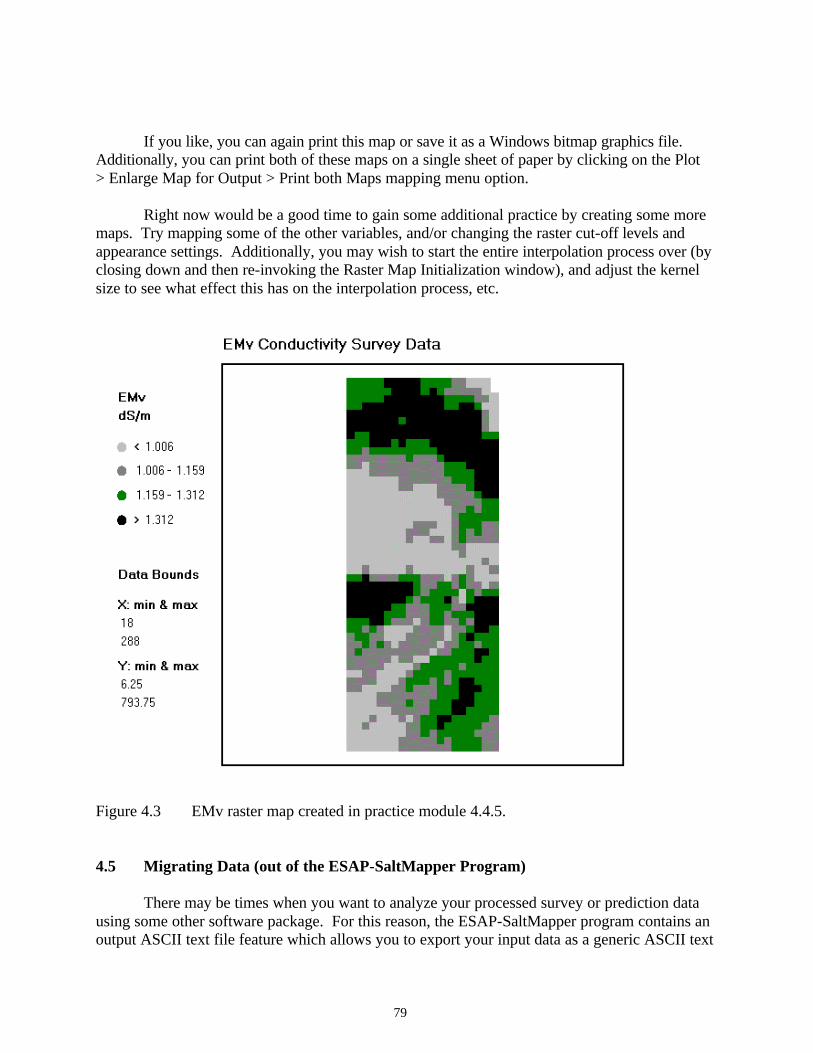
79

If you like, you can again print this map or save it as a Windows bitmap graphics file. Additionally, you can print both of these maps on a single sheet of paper by clicking on the Plot > Enlarge Map for Output > Print both Maps mapping menu option. Right now would be a good time to gain some additional practice by creating some more maps. Try mapping some of the other variables, and/or changing the raster cut-off levels and appearance settings. Additionally, you may wish to start the entire interpolation process over (by closing down and then re-invoking the Raster Map Initialization window), and adjust the kernel size to see what effect this has on the interpolation process, etc.

Figure 4.3 EMv raster map created in practice module 4.4.5. 4.5 Migrating Data (out of the ESAP-SaltMapper Program) There may be times when you want to analyze your processed survey or prediction data using some other software package. For this reason, the ESAP-SaltMapper program contains an output ASCII text file feature which allows you to export your input data as a generic ASCII text

80

file. This section describes how to use this export feature. 4.5.1 Creating and Saving ASCII Text Files You can use the ASCII File Output window to generate a comma delimitated, output ASCII text file of an ESAP-SaltMapper data file. To invoke this window, click on the File > Create Output Data File main menu option. Before saving your ASCII text file, you should choose the appropriate decimal degree accuracy for the output data columns. The default is 2 decimal degrees (i.e., the number 1 will be printed as 1.00); however, you can set the accuracy from 1 to 4 decimal degrees, respectively. You should also specific data columns you wish to place into the output data file. You need to select (i.e., check) at least one data column in order to create and save an ASCII output text file. By default, the site ID number, x-coordinate, and y-coordinate data columns will be initially selected (the row number column will also be selected if you are working with a transect type survey or prediction file). These columns can be de-selected if you wish. Finally, to create the output data file, you must specify the output path and file name and then save the file. You can use the Specify Output File Name and Save File command buttons to perform these actions. 4.5.2 Practice Module (Exporting the BV10data.svy Data File) In this final practice module you will learn how to export and save the BVWDdata.svy data as an ASCII text file. To invoke and display the ASCII File Output window, click on the File > Create Output Data File main menu option. Once this window appears, you can set your decimal degree accuracy and then select the desired data columns. For this example, set the degree accuracy to 3, and select (i.e., check) the x-coordinate, y-coordinate, EMv, EMh, and EM-ratio data column check boxes. (To de-select the site ID and row number columns, simply click on their corresponding check boxes.) Now, click on the Specify Output File Name command button. When the File Open window appears, change the default directory to esap2 (or some other directory, if desired), type in the name "bvwd_out" (without the quotes), and click on the Open button. Then click on the Save File command button (located back on the ASCII File Output window). The ESAP-SaltMapper program should then export 1015 lines of data to your output file. When the export process is finished, you should see the following message:

Output ASCII file saved to C:\US_Salinity_Lab\esap2\bvwd_out.txt This message is reminding you where your output data file is on your hard-drive, and confirming that the export process was completed successfully.

81

5.0 ESAP-Calibrate Software Program 5.1 ESAP-Calibrate Program Overview The following section gives an overview of the ESAP-Calibrate software program, including a review of how the program functions and a description of the main menu bar layout. 5.1.1 Program Description What is ESAP-Calibrate ESAP-Calibrate is a comprehensive data analysis program which can be used to convert raw conductivity data to soil salinity data via either stochastic calibration or deterministic techniques; i.e., by using an empirically fit regression model or the DPPC (Dual Pathway Parallel Conductance) equation, a.k.a. the Rhoades conductivity model. Additional capabilities of the ESAP-Calibrate program currently include: a) the ability to use stochastic calibration models to predict levels of secondary soil properties (provided secondary sample data has been acquired); b) the ability to use the deterministic DPPC model to estimate the theoretical strength of correlation’s between raw conductivity and ECe, SP, volumetric water content, and/or other secondary sample data that may have been acquired during the sampling process; c) the ability to produce 1D profile data graphs and perform bivariate profile data correlation analysis; d) the ability to fully automate the stochastic calibration (regression modeling) process. The ESAP-Calibrate program has been designed to operate on two types of input data; survey data (i.e., *.svy data files produced by the ESAP-RSSD program) and calibration sample data (i.e., the laboratory analyzed soil sample data collected from a set of calibration sample sites). The latter data is referred to as "soil profile" data (or simply "profile" data) in this manual, because the ESAP-Calibrate program can import and process calibration soil sample data from multiple sample depths. (In version 2.01, up to 6 sampling depths can be associated with each calibration sample site.) All calibration sample data imported into the ESAP-Calibrate program should be saved as a permanent ESAP-Calibrate *.pro (profile) data file. This feature allows you to quickly and easily import the same data back into the program during any future data analysis sessions.

82

Additionally, whenever you generate output spatial prediction data, you should save this data as a permanent *.prd (prediction) data file. These *.prd data files can then in turn be imported into the ESAP-SaltMapper program and used to create either 1D transect plots or 2D raster maps. How does the ESAP-Calibrate Program Work As discussed above, the ESAP-Calibrate program contains a number of modeling and analysis features. In the ESAP-Calibrate program, these features are separated into two general categories; stochastic methods and deterministic methods, as shown below: Stochastic Methods (methods which require profile data): (1) profile shape / magnitude analysis (1D profile plots) (2) standard correlation analysis (bivariate correlation plots) (3) DPPC correlation analysis (conductivity influence analysis) (4) stochastic calibration modeling (spatial regression modeling) Deterministic Methods (methods which do NOT require profile data): (5) deterministic conversion of conductivity into salinity Four of the five primary analysis methods are stochastic (statistical) methods, which in practice means that they can only be used if profile (calibration) data have been collected. In contrast, you do not need to acquire any profile data to use the deterministic conductivity to salinity conversion routine. Table 5.1 shown below describes the type of data each analysis method is designed to work on. Table 5.1 Data requirements for each analysis method.

Analysis Method

Survey (conductivity) data

required

Profile (calibration) data

required profile shape / magnitude analysis No Yes

standard correlation analysis No Yes

DPPC correlation analysis optional Yes

stochastic calibration modeling Yes Yes

deterministic conversion routines Yes No

In the ESAP-Calibrate program, each analysis method is designed for a specific purpose. For example, a profile shape / magnitude analysis is designed to produce 1D profile plots. A 1D profile plot is a graphical representation of your calibration sample (profile) data, where the magnitude of a specific soil sample variable is plotted against the sampling depth, and data

83

points from specific soil cores are joined (connected) together by lines. For sample soil salinity data, a 1D profile plot can be used to display the shape of the salinity profile with respect to the overall magnitude of the average salinity level for each sample core (thus allowing you to qualitatively infer the net direction of water flow under equilibrium conditions). Likewise, a standard correlation analysis is designed to produce bivariate correlation plots and correlation statistics. This analysis allows you to visualize and quantify the correlation structure between any two input columns of profile data. For example, you could plot and examine the correlation structure between your sampled soil salinity and soil texture. One of the most useful procedures contained within the ESAP-Calibrate program is the DPPC correlation analysis. A DPPC correlation analysis can be performed on any valid DPPC profile data file, either before or after merging such a profile data file with the corresponding survey data. This analysis allows you to calculate (i.e., estimate) a set of soil conductivity readings, based on your input sample salinity, texture, and water content data values. These calculated soil conductivity readings can then be compared to each column of input soil data, thus allowing you to see how well the calculated conductivity correlates with each soil variable. If you have survey data associated with these profile sites, then you can also look at the correlation between your calculated and measured (i.e., true) conductivity readings. The final stochastic procedure contained within the ESAP-Calibrate program is the stochastic calibration procedure. This procedure allows you to generate spatially referenced regression models, which in turn use the acquired conductivity survey readings to predict the values of one or more soil variables at each survey site within your field (or survey area). These models can also be used to estimate the average level of each soil variable within the field, and calculate a number of additional, useful prediction statistics. Furthermore, these models can be used to generate predictions of your soil variable across multiple sampling depths, provided you acquire multiple depth calibration data. If you are only interested in estimating the soil salinity pattern across your survey area, and you can not afford to acquire any calibration sample data, then you can use the deterministic conversion algorithm. This algorithm converts conductivity data into salinity data using a two-step process. First, raw instrument conductivity is converted into depth specific soil conductivity (ECa, for a given depth). Next, this ECa data is converted into estimated soil salinity data using a linear version of the DPPC model. All of the analysis procedures described above are explained in detail within the remainder of this chapter.

84

5.1.2 Navigating the ESAP-Calibrate Main Menu Bar Main Menu Bar: Layout The ESAP-Calibrate main menu bar is located in the upper left corner of the main program window. The full layout for this menu bar system is shown below. Main level Sub-Level 2 Sub-Level 3 File --> Import Data File | | | --> Import a Survey data file | --> Import a Profile data file | --> Edit or Validate Profile Data | --> View / Print Project Output Files | --> Exit Calibrate --> Stochastic Methods | | | --> Profile Shape / Magnitude Analysis | --> Standard Correlation Analysis | --> DPPC Correlation Analysis | --> Spatial MLR Analysis | --> Deterministic Methods | --> Conductivity to Salinity Help --> About ESAP-Calibrate | --> ESAP Interface Controls | | | --> Reset default Text Editor | --> OnLine Help --> What is ESAP-Calibrate --> Navigating the Main Menu --> Frequently Asked Questions (FAQ) Main Menu Bar: Menu Item Descriptions The profile menu contains 3 menu bar items; File, Calibrate, and Help. You will use the File menu to access all the data input/output and validation routines, the Calibrate menu option to access all of the data analysis routines, and the Help menu to access the main ESAP program

85

help files. Additional help file documentation is available for nearly all ESAP program routines; this documentation can be accessed by double clicking on the OnLine Help file button within whatever window is currently activated (the OnLine Help button is the small button displaying a capital "H", usually located in the lower right hand corner of the window). Brief descriptions of the sub-level menu items (located beneath the 3 main program menu bar items) are given below: ( from within File ) Import Data File: Import a survey data file Select this option to invoke and display the Survey Data File Import window, which can in turn be used to import a previously created ESAP *.svy survey data file. Import Data File: Import a profile data file Select this option to invoke and display the Profile Data File Import window, which can in turn be used to import either a previously created ESAP profile (*.pro) data file, or new calibration sample data (stored in a suitably formatted ASCII text file). Edit or Validate Profile Data Select this option to invoke and display the Summarize / Edit / Save Profile Data window. The options contained within this window can be used to validate and save newly imported calibration sample data as an ESAP profile (*.pro) data file. All calibration sample data must be validated (i.e., examined) by ESAP the first time it is imported into the program. Additionally, once you save your data as a *.pro data file, you will never need to validate it again, or specify the file structure, etc. View / Print Project Output Files Select this option if you would like to view and/or print any of the ESAP generated output text files currently residing in any of your active project directories. Exit Select this menu option to exit the ESAP-Calibrate program. ( from within Calibrate ) Stochastic Methods: Profile Shape / Magnitude Analysis Select this menu option to invoke and display the 1D Profile Display window, which can in turn be used to create 1D profile plots. A 1D profile plot is a graphical representation of your profile data, where the magnitude of a specific soil sample variable is plotted against the

86

sampling depth, and data points from specific soil cores are joined (connected) together by lines. Stochastic Methods: Standard Correlation Analysis Select this menu option to invoke and display the Standard Correlation Analysis window, which can in turn be used to create bivariate correlation plots and statistics. This analysis allows you to visualize and quantify the correlation structure between any two input columns of profile data. Stochastic Methods: DPPC Correlation Analysis Select this menu option to invoke and display the DPPC Profile Data Correlation Analysis window (DPPC-PDCA window), which can in turn be used to perform a DPPC correlation analysis. A DPPC correlation analysis can be performed on any valid DPPC profile data file, either before or after merging such a profile data file with the corresponding survey data. This analysis allows you to calculate (i.e., estimate) a set of soil conductivity readings, based on your input sample salinity, texture, and water content data values. These calculated soil conductivity readings can then be compared to each column of input soil data, thus allowing you to see how well the calculated conductivity correlates with each soil variable. If you have survey data associated with these profile sites, then you can also look at the correlation between your calculated and measured (i.e., true) conductivity readings. Stochastic Methods: Spatial MLR Analysis (Stochastic Calibration) Select this menu option to invoke and display the Stochastic Calibration Modeling window. The various routines and procedures contained within this window can be used to generate spatially referenced regression models, which in turn use the acquired conductivity survey readings to predict the values of one or more soil variables at each survey site within your field (or survey area). These models can also be used to (1) estimate the average level of each soil variable within the field, (2) calculate various additional prediction statistics, and (3) generate predictions of your soil variable across multiple sampling depths, provided you acquire multiple depth calibration data. Deterministic Methods: Conductivity to Salinity Select this menu option to invoke and display the Deterministic Conductivity to Salinity Conversion window, which can in turn be used to initialize and invoke the deterministic conversion algorithm. This algorithm converts conductivity data into salinity data by first converting the raw instrument conductivity into depth specific soil conductivity (ECa, for a given depth), and then by estimating the soil salinity levels from this ECa data using a linear version of the DPPC model.

87

( from within Help ) About ESAP-Calibrate Select this option to display the ESAP information window. ESAP Interface Controls: ReSet default Text Editor You may use this option to change the default text editor used by ESAP to display and print all ESAP generated text files (and/or print any ESAP help file). At program start-up, the default text editor package is set to "c:\windows\write.exe". OnLine Help: What is ESAP-Calibrate Select this option to display the introductory help documentation. This is the help documentation you should read first if you have never used the ESAP-Calibrate program before. This documentation explains what the ESAP-Calibrate program does and how the program works. OnLine Help: Navigating the Main Menu This documentation explains how to use the Main menu bar, and describes the menu bar features. OnLine Help: Frequently Asked Questions (FAQ) This is the help documentation you should read if need more detailed information about how to use the various program features. For example, refer to this documentation if you don't understand what sort of input data each analysis procedure is designed to work on, or if you need advice on where to find more detailed explanations for each procedure, etc. 5.2 Importing Previously Saved ESAP Data Files This section describes how to import previously saved ESAP-RSSD survey (*.svy) and ESAP-Calibrate profile (*.pro) data files. 5.2.1 Importing ESAP-RSSD Survey (*.svy) Data Files You should use the Survey Data Import Window to import your *.svy data file into the ESAP-Calibrate program. This window can be invoked and displayed using the File > Import Data File > Import a Survey Data File main menu option. In order to successfully import your data file, you must perform the following two steps. First, you must set the current project; i.e., you must identify which project your *.svy data file

88

resides in. This can be done by clicking on the appropriate project name listed in the Set Current Project list box. Second, you must specify the path and filename of your input file. This can be done by typing in the appropriate information into the Path / Filename input text box, or by using the Browse button to locate your input file. Once you have performed these steps, click on the OK button to import your *.svy data file. If your input data file does not import properly, then the error message listed below will appear and the data import process will be aborted. Error! Invalid path/filename or file corruption error detected. This error will be generated if you attempt to import any file type other than an ESAP generated *.svy data file. The error will also occur if your input data file has become accidently corrupted (in this latter case, you should use the ESAP-RSSD program to re-generate your input data file). 5.2.2 Importing ESAP-Calibrate Profile (*.pro) Data Files In the ESAP-Calibrate program, the term "profile data" is synonymous with calibration sample data. In other words, a profile data file is actually a file containing laboratory measurements made on your calibration soil samples, such as soil salinity, SP, gravimetric or volumetric water content, etc. In practice, this data file should contain at least some measurements which you wish to calibrate your soil conductivity survey data to. Additionally, the sampling locations (of the analyzed soil samples) should generally correspond to one or more sampling designs generated within the ESAP-RSSD program. You can use the Profile Data File Import Window to import either a previously saved profile data file or new calibration sample data (stored in a suitably formatted ASCII text file). This window can be invoked and displayed by clicking on the File > Import Data File > Import a Profile Data File main menu option. To import a previously saved ESAP-Calibrate profile data file (a file having a *.pro extension), you simply need to set the current project directory and then specify the path and filename of your input file. To specify the current project, click on the appropriate project name listed in the Set Current Project Directory list box. Next, make sure that the input file status is set to "previously saved Profile data file" (the file status frame should default to this option). Then type in the appropriate information into the Path / Filename input text box, or use the Browse button to locate your input file. Once you have performed these steps, click on the OK button to import your *.pro data file. If a file import error message occurs when you attempt to read in a previously saved profile data file, then this *.pro data file has become corrupted. In such a scenario you will need to re-import the calibration sample data associated with this file and re-save it. (Note: previously saved *.pro files can be corrupted if you attempt to edit these data files outside of the ESAP-Calibrate program.)

89

5.2.3 Practice Module (Importing ESAP Data Files) If you have not already done so, start up the main ESAP-95 splash screen by clicking on the ESAP-95 prompt listed within the Programs drop-down menu system (i.e., click on Start > Programs > Esap95). Once the splash screen has displayed, click once on the ESAP-Calibrate command button to invoke the Calibrate program. Once the ESAP-Calibrate main menu screen is fully displayed, click on the File >Import Data File > Import a Survey Data File main menu option. This will cause the Survey Data File Import window to be displayed. You will be using the data stored in the Training2 project during this practice module, so click once on the Training2 project name and make this your active project. Now click on the file browse button; when the File Browse window appears you should see a file called sk13data.svy. Double-click on this file name, and then click once on the OK command button after you return to the Survey Data File Import window. The ESAP-Calibrate program should then import this survey data file and print out the following summary information to the main program screen: Field ID Code: sk13 File Type: Transect Sig Trans: log # of survey sites: 100 # of sig columns: 2 Sig labels: lnEMv, lnEMh In addition to the above information, the input file project and full file path information should also be displayed. To import the corresponding profile data file information, click on the File >Import Data File > Import a Profile Data File main menu option. This will cause the Profile Data File Import window to be displayed. Make sure the input file status is defined as "previously saved profile data file", and then set the current project to Training2 (again by clicking once on the Training2 project name in the Project Directory display window). Now click on the file browse button; when the File Browse window appears you should see a file called sk13_lab97.pro. Double-click on this file name, and then click once on the OK command button after you return to the Profile Data File Import window. The ESAP-Calibrate program should then import this profile data file and print out the following summary information to the main program screen: # of sample sites: 15 # of sample depths: 4 # of data columns: 8 Furthermore, you can display additional information about the profile data file by clicking on the Column Info command button. This additional information will include the profile data file type, individual column labels and units, and the data file status.

90

As should be obvious, it is relatively simple to import previously saved survey or profile data into the ESAP-Calibrate program. All you really need to remember are the file names and where each file resides (i.e., which project). 5.3 Importing New Data Files This section describes how to import new calibration sample data into the ESAP-Calibrate program. Included here is a description of the two types of profile data files which can be created from calibration sample data, and the formatting and column structure requirements of each input file type. 5.3.1 The Two Types of Laboratory Profile Data In the ESAP-Calibrate program, calibration sample data can be imported as one of two profile data file types: DPPC or Generic. However, in either case, your calibration data must first be stored in a comma or space delimited ASCII text file. Note also that you must create this input file using some other program such as a text editor or spreadsheet software, before importing it into the ESAP-Calibrate program. The ESAP-Calibrate program can not create this ASCII data file for you.

This being said, the column structure of the input calibration data represents the primary difference between the two profile data file types. By design, all DPPC type input data files have the following general column structure: DPPC Column Structure: Column # 1 site_ID (required) 2 sample depth (midpoint) (required) 3 salinity (required) 4 texture (required) 5 water content (required) 6 bulk density (optional) 7-10 secondary soil measurements (optional) Additionally, the input data file must be double-sorted; first by the site_ID numbers, and then by the sampling depths. For example, suppose you collected calibration sample data from 3 depths at each of 10 sites across the survey area. Then your input data file might look like the (abbreviated) data file shown below. 7 0.15 2.33 56.7 21.1 7 0.45 5.67 53.2 20.4 7 0.75 9.41 47.7 19.9 18 0.15 1.67 66.6 24.4 18 0.45 4.44 58.2 23.9 18 0.75 6.93 51.1 17.7

91

↓ 181 0.15 3.56 62.3 23.3 181 0.45 6.32 69.9 27.5 181 0.75 8.48 49.9 18.8 In the above example, the first sample site comes from survey site number 7, the last sample site comes from survey site number 181, the sampling depths come from the 0.0-0.3, 0.3-0.6, and 0.6-0.9 meter depths, and the 3rd, 4th, and 5th data columns represent soil salinity (dS/m), saturation percent (%), and gravimetric water content (%). Note that the input data is sorted first by site, and then by depth for each site. However, there are no other specific formatting requirements; i.e., your individual data columns do not have to follow any special format, nor do the numbers need to be column aligned (like the data shown above). If your laboratory data file you wish to import does not include measurements of salinity, texture, and soil water content, then you should import it as a Generic file type. By design, all generic type input data files have the following general column structure: Generic Column Structure: Column # 1 site_ID (required) 2 sample depth (midpoint) (required) 3 1st soil measurement (required) 4-10 additional soil measurements (optional) Hence, in a Generic file, your input data in columns 3 through 10 can represent any soil variable you may have measured. However, the input data file must still be double-sorted; first by the site_ID numbers, and then by the sampling depths. For example, suppose you collected sample data from 3 depths at each of 10 sites across the survey area, and measured two soil properties on each sample. Then your input data file might look like the (abbreviated) data file shown below. 17 0.15 23.4 12.3 17 0.45 26.6 10.9 17 0.75 35.5 15.6 28 0.15 41.1 19.9 28 0.45 47.7 22.2 28 0.75 54.4 21.1

↓ 188 0.15 17.4 10.7 188 0.45 14.3 11.6 188 0.75 22.2 13.8 In the above example, the first sample site comes from survey site number 17, the last sample site comes from survey site number 188, the sampling depths come from the 0.0-0.3, 0.3-0.6, and 0.6-0.9 meter depths, and the 3rd and 4th data columns represent your 2 soil measurements collected at each sample site. Note once again that (1) the input data is sorted first by site, and then by depth for each site, and (2) arbitrary data formatting is acceptable.

92

All DPPC or Generic type input data files must contain sample site ID numbers in column 1 and sample depth values in column 2. Furthermore, all DPPC type files must contain soil salinity measurements in column 3 (ECe readings in either dS/m or mS/m units), texture measurements in column 4 (either SP or %Clay), and water content measurements in column 5 (either volumetric or gravimetric). If it has been obtained, then bulk density data should be placed into column 6. Any additional secondary soil measurements (such as SAR, boron, nitrate, cation or anion levels, etc.) can be placed into columns 7 through 10. If no bulk density data is present, then the first additional secondary soil measurement should appear in column 6, rather than column 7. In Generic type profile data files, your soil measurements begin in column 3 and you can include up to a total of 8 soil measurement columns in your file (placed into columns 3 through 10). You must include at least one soil measurement column (in column 3), but columns 4 through 10 are optional. Finally, if your input soil data includes measurements of salinity, texture, and water content then you should import this data as a DPPC type profile data file. This in turn will allow you to perform a DPPC correlation analysis on your input profile data (a DPPC correlation analysis can not be performed on generic type profile data files). On the other hand, if your input data does not contain salinity, texture, and water content readings at every sample site then you can not import it as a DPPC type profile data file (you must use the Generic file format instead). 5.3.2 Importing Your Data (Setting File Type and Column Structure Specifications) Once you have created and saved your ASCII data file (which contains your calibration sample data), you can import it into the ESAP-Calibrate program. To import a new calibration sample data file, you should again use the Profile Data File Import window. This window can be invoked and displayed by clicking on the File > Import Data File > Import a Profile Data File main menu option. After the Profile Data File Import window has displayed, you should perform the following steps. First, change the Input File Status to "new Profile data file". After you do this, a Project Status frame will appear. If you wish to create a new project then click on the "create a new Project Directory" option, else move down to the Set Current Project Directory frame and select your desired project (i.e., the project you wish to store your laboratory data in). Once you have either set or created your project, you can then define your input data file type. If you wish to import a DPPC file type, then click once on the DPPC command button (located inside the Define Input File Format frame). Else, click on the Generic command button to define a Generic file type. If you click on the DPPC command button, then the DPPC Profile Data File Format Sheet should appear. You can then use the controls on this sheet (i.e., contained within this window) to specify the exact structure of your input file. Note that you will need to specify the following information:

93

(1) the number of sample sites (i.e., sample cores), (2) the number of sampling depths associated with each site (from 1 to 6), (3) the number of secondary variables (from 0 to 4) measured on each sample (i.e., variables other that salinity, texture, water content, and bulk density), (4) the sampling depth units (such as inches, feet, or meters, etc.), (5) the salinity (ECe) units, which should be either dS/m or mS/m,

(6) the type of soil texture (SP or % Clay) and water content measurements (gravimetric or volumetric), (7) whether or not bulk density measurements have been acquired, and (8) the column labels and measurement units for each secondary variable, if any. Once all of this information has been specified, you can use the Review Format command button to review your input information, and the OK command button to save this information. If you click instead on the Generic command button, then the Generic Profile Data File Format Sheet will appear. As before, you should then use the controls on this sheet to specify the exact structure of your input file. Note that you will need to specify the following information: (1) the number of sample sites (i.e., sample cores), (2) the number of sampling depths associated with each site (from 1 to 6), (3) the total number of input columns (from 3 to 10, this includes the site ID and sample depth data columns) (4) the sampling depth units (such as inches, feet, or meters, etc.), and (5) the remaining column labels and measurement units for each soil variable. Once all of this information has been specified, you can again use the Review Format command button to review your input information, and the OK command button to save this information. After you click on the OK command button (in either Format Sheet), you will return to the Profile Data File Import window. You should now use the Browse command button to locate and open your calibration sample data file, and then click on the Import window OK button to import your data. As the ESAP-Calibrate program imports your data, it will perform some preliminary data sorting checks. One or more input data read errors will occur if your data is not properly sorted, or your data file format is mis-specified. If this occurs, you should try to identify and fix the problem(s) before attempting to re-import the file. Note that file mis-specification errors can generally be fixed inside of the ESAP-Calibrate program by re-displaying the appropriate Format Sheet and changing the incorrect specifications. However, data sorting errors will need to be fixed outside of the ESAP-Calibrate program using some other type of software.

94

Note also that the ESAP-Calibrate program does NOT have the ability to selectively import a subset of data columns from a larger data file. In other words, suppose your ASCII data file contains 12 columns, but you only wish to import a subset of 6 columns. In such a situation, you can NOT import the 12 column data file directly into the ESAP-Calibrate program. Instead, you must first create a new data file which only contains the 6 columns of data which you wish to use, and then import this smaller data file. 5.3.3 Practice Module (Importing New Data) For this practice module you will use the ASCII data file called sk13_97.lab, which is located in the Training2 project. As with previously saved profile data, you first need to invoke and display the Profile Data File Import window (in the identical manner as you did in Practice module 5.2.3). However, once this window displays, you need to perform the following extra steps (when you import new calibration sample data for the first time). First, set the input file status to "new profile data file". Next, define the project status; i.e., decide whether you wish to create a new project directory, or set the current project directory. If you would like to make a new project, then select the "create a new Project..." option, type in a valid Project name, and then click on the Create command button. If you wish to use an existing project, then select the "set the current Project..." option and click on the desired project name in the Set Project display window. (Note: use the Training2 project for this practice module, if you decide not to create a new project.) Once your project has been identified, you next need to define the input file format. If you intend to import a DPPC type data file then click once on the DPPC command button; otherwise click on the Generic command button to import a generic type data file. Lets begin by importing the sk13_97.lab data file as a generic file, so click once on the Generic button. This should invoke and display the Generic Profile Data File format sheet, which should be filled in with the following information: Number of sample sites: 15 Number of sampling depths per site: 4 Total number of input columns: 7 Column # Units 2 meters Column # Label Units 3 ECe dS/m 4 SP % 5 grav H2O % 6 SAR none (or leave blank) 7 Boron ppm

95

After you have entered this information, click once on the format sheet OK command button to return to the Profile Data File Import window. You should now identify your input ASCII data file by clicking on the Browse command button (you will find the sk13_97.lab data file in the Training2 project directory). Once you have opened this data file (using the File Browse window), click once on the Import window OK command button to initiate the data import process. After the data has been successfully imported, the ESAP-Calibrate program will automatically display some summary file information on the main program window (and also remind you that this file has not yet been saved as a permanent profile data file). The directions given above should be followed whenever you need to import a generic type data file. However, the sk13_97.lab data file is actually a valid DPPC type data file, so now you should re-import this data as a DPPC file type. To do this, open up the Profile Data File Import window again, and set or create your project. Once you are ready to define the input file format, click on the DPPC command button. This will invoke and display the DPPC Profile Data File format sheet, which should be filled in with the following information: Number of sample sites: 15 Number of sampling depths per site: 4

Number of secondary variables measured per site: 2 Column # Units 2 meters 3 dS/m Column #4: check the “SP” check-box Column #5: check the “Gravimetric” check-box Column #6: check the “NOT present” check-box Column # Label Units 6 SAR none (or leave blank) 7 Boron ppm After you have entered this information, click again on the format sheet OK command button to return to the Profile Data File Import window. Now, as before, you should identify the name and location of your ASCII data input file, and then import the data (in the exact same manner as you just did during the generic file import process). After the sk13_97.lab data has been re-imported, click on the ESAP-Calibrate main window Column Info command button. When the detailed data file information is displayed, verify that the defined file type is "DPPC" and that the current data file status is reported as "NOT validated". Also verify that the main window information reports that this file is "not yet saved". In the next section (section 5.4), you will learn how to validate and save this new DPPC profile data file.

96

5.4 Editing and Validating New Profile Data The following section describes how to use the ESAP-Calibrate software program to validate, and if necessary edit a newly imported calibration sample data file. This section also explains how to create a profile (*.pro) data file from imported calibration sample data. 5.4.1 Validating New Laboratory Profile Data After you first import a new calibration sample data file (of type DPPC or generic), you will need to validate this data. If you have imported a DPPC type data file, this validation routine will perform a number of data checks on the input salinity, texture, and water content data columns, and also the bulk density data column (if present). If you have imported a generic type data file, then this validation routine will simply summarize your input data. Regardless of the type of input calibration data file you import (DPPC or generic), you must run this validation routine once before you can save your calibration data (as an ESAP-Calibrate *.pro data file) and/or use any of the Stochastic Data Analysis Methods. The validation routine can be invoked by clicking on the File > Edit or Validate Profile Data main menu option. This will invoke and display the Summarize / Edit / Save Profile Data window, which can then be used to invoke the validation, editing, and file saving routines. If you have imported a DPPC type data file, you can perform up to three data column conversion routines when you validate your data. (Note: if you are validating Generic profile data, then all of the options discussed below will be disabled.) These conversion routines can be invoked by checking the appropriate check boxes shown in the DPPC Profile Data Options frame. If selected, they will perform the following actions: Convert %Clay To Estimated SP: If your input texture data is percent clay, then you can convert this data into estimated SP values by highlighting this check box. (Note: this action will permanently replace the % clay data with estimated SP data values.) Convert Gravimetric H2O To Estimated Volumetric H2O: If your input water content data is measured on a gravimetric basis, then you can convert this data into estimated volumetric water content values by highlighting this check box. (Note: this action will permanently replace the gravimetric water content data with estimated volumetric water content data values.) Estimate % H2O Relative to FC (Field Capability): If desired, ESAP can calculate the percent water content relative to estimated field capacity, and

97

store this information into a new data column. This option is available regardless of the type of input water content data (volumetric or gravimetric). Once you have indicated any desired conversion options (if applicable), click once on the Compute Summary Statistics command button to invoke the data validate routines. If you are working with generic data, then the ESAP-Calibrate program will simply summarize your input calibration sample data. If you are working with DPPC data and one or more data boundary errors are detected, then you can view a listing of these errors by clicking on the View Summary Statistics command button. Even if there are no boundary errors detected, we recommend that you view this log file since this is where your profile summary statistics will be reported. (We also recommend that you generate a print-out of this file for your records). If you feel that one or more inputted data values are in error, then you have the option of editing these values. Note that a separate data editing window can be invoked and displayed by clicking on the Edit Data command button, refer to section 5.4.2 for more details. If all of your calibration sample data passes the data validation tests, then you should save this data as an ESAP-Calibrate profile (*.pro) data file using the command buttons contained in the File Save Options frame. First, click on the Specify Output Filename button to specify a unique name for your *.pro data file. Once you have done this, you should then click on the Save Data command button to save (i.e., create a permanent copy of) this profile data file. In general, we recommend that you always save any input calibration sample data you wish to analyze as a permanent *.pro data file. Previously saved profile data files can be quickly imported into the ESAP-Calibrate program, because ESAP can automatically recognize their format structure (see section 5.2.2). 5.4.2 Editing Laboratory Data The Data Editing window can be used to edit any input calibration sample data values, and/or change the data column labels or column units. To invoke and display this window, click once on the Edit Data command button (from within the Summarize / Edit / Save Profile Data window). You can edit both your calibration sample data values and your data column labels or units, if necessary. You are free to change any or all of your column labels and /or column units; simply select the appropriate text box and type in the new label or unit. When editing calibration sample data, note that you can not change any site ID or sample depth data values. However, all other data values can be changed as necessary. To edit calibration data, first select the proper data record and then type in the new values. Note that you can scroll through your data records using either the Increment / Decrement command buttons, or you can jump to a specific record using the Jump command button.

98

Once you have finished editing your data (or column labels), click first on the appropriate OK command buttons and then on the Finished button to return to the Summarize / Edit / Save Profile Data. You should then re-validate your calibration sample data file by clicking on the Compute Summary Statistics button. Note: As stated above, you can not edit either the sample site ID or sample depth data values. This restriction has been built into the program, on purpose, to prevent you from accidently corrupting any site ID or sample depth records. If one or more of these values are in error then you must exit the ESAP-Calibrate program, correct these values in your raw profile data file, and then re-import this data. 5.4.3 Practice Module (Validating Laboratory Profile Data) This practice module demonstrates how you should validate new calibration sample data. If you have not already performed practice module 5.3.3, you should do so now; (you need to import the sk13_97.lab data as a DPPC data file before you can begin this module). All new calibration sample data files must be validated using the Summarize / Edit / Save (SES) Profile Data window. To invoke and display the SES window, click on the File > Edit or Validate Profile Data main menu option. If you are validating a DPPC data file (as in this practice example), you will see up to 3 data conversion check box options enabled and displayed within the SES window. In this example, two options are enabled: (1) convert gravimetric H2O to estimated volumetric H2O, and (2) estimate % H2O relative to field capacity. These conversions are optional, but for this example you should go ahead and activate (i.e., check) both of these check boxes. This will instruct the ESAP-Calibrate program to replace your gravimetric water content data with estimated volumetric readings, and also to produce a new column of estimated % water content relative to field capacity (%H2O | FC) readings. After you've activated any applicable check boxes, you simply need to click once on the Compute Summary Statistics command button. If no boundary error conditions are detected, then both a View Summary Statistics command button and a File Save Options frame will appear. If one or more errors do occur, the ESAP-Calibrate program will notify you with a warning message and inform you to use the View Summary Statistics command button to display the error messages. If the reported errors can be fixed by editing specific laboratory data readings, then you should click on the Edit Data command button to invoke and display the Data Editing window (see section 5.4.2). Note that during this practice session, no errors should occur when you compute the summary statistics on the sk13_97.lab data file. We strongly recommend that you make it a practice to save all new calibration sample data files as permanent *.pro profile files. You should use the Specify Output Filename command button to specify your permanent output file name, and the Save File command button to save the file. As you have already learned, previously saved profile data files can be imported back into the ESAP-Calibrate program much more quickly than new calibration sample data files (during any future analysis sessions). You should also print out the summary statistics report if

99

you want to retain a hard-copy record of when your calibration data was first imported into the ESAP-Calibrate program. 5.5 ESAP-Calibrate Deterministic Salinity Conversion Modeling The ESAP-Calibrate program allows you to covert conductivity to salinity via either deterministic or stochastic modeling techniques. This section explains how the deterministic conversion routines work, and what sort of survey information you need to collect (in addition to your soil conductivity data) in order to achieve the highest possible conversion accuracy. 5.5.1 How Does a Deterministic Conversion Work In the ESAP-Calibrate program, soil conductivity can be converted into estimated soil salinity data using a deterministic conversion algorithm. This algorithm converts conductivity data into salinity data using a two-step process. First, raw instrument conductivity is converted into depth specific soil conductivity (ECa, for a given depth). Next, this ECa data is converted into estimated soil salinity data using the linear version of the DPPC model. The following information is required to convert raw conductivity into ECa readings: (1) the average soil temperature, (2) the conductivity instrument signal correction factors (if applicable), and (3) the conductivity to ECa conversion formula type and parameter estimates. Then, to convert ECa data into soil salinity, you must additionally specify the field average SP, bulk density, and % water content relative to field capacity. Because this algorithm uses a deterministic approach, no soil salinity prediction errors are generated during the conversion process. Additionally, caution is urged when using this approach, since serious errors in one or more of the input parameters can lead to significant ECe estimation errors. In general, if you have acquired soil samples, we recommend that you use the regression modeling approach to statistically predict the soil salinity levels from the conductivity survey data (i.e., stochastic calibration modeling). If you are unfamiliar with the DPPC model, you may wish to refer the discussion of the DPPC equation given in section 5.8. Also, please note that this deterministic conversion algorithm can only process (i.e., estimate) salinity data within a single depth. If you wish to calculate the salinity levels across multiple profile depths, then you will need to run this algorithm in an iterative manner.

100

5.5.2 Navigating the Deterministic Conductivity to Salinity (DCS) Menu DCS Menu Bar: Layout The ESAP-Calibrate Deterministic Conductivity to Salinity menu bar is located in the upper left corner of the DCS program window. This window can be invoked and displayed by clicking on the Calibrate > Deterministic Methods > Conductivity to Salinity main menu option. The full layout for this menu bar system is shown on the following page. Main level Sub-Level 2 Parameters --> Set Conductivity Parameters | --> Set Soil Parameters Calculate --> Convert Conductivity to Salinity Help --> How does a Deterministic Conversion work | --> Navigating the DCS Menu Exit --> Return to Main Menu DCS Menu Bar: Menu Item Descriptions The DCS menu contains 4 menu bar items; Parameters, Calculate, Help, and Exit. You can use the Parameters menu to set your conductivity and soil parameters, the Calculate menu to convert your conductivity data to estimated salinity data, and the Help menu if you wish to access any DCS help files. Brief descriptions of the sub-level menu items (located beneath the 4 main program menu bar items) are given below: ( from within Parameters ) Set Conductivity Parameters Select this option to define and input your raw conductivity to ECa conversion information. This information consists of (1) the average soil temperature, (2) conductivity instrument signal correction factors (if applicable), and (3) the conductivity to ECa conversion formula type and parameter estimates. Set Soil Parameters Select this option to define the values of the soil parameters for use in the DPPC

101

equation; i.e., to define the soil texture, bulk density, and water content level. ( from within Calculate) Convert Conductivity to Salinity Select this option to convert your conductivity survey data into estimated soil salinity data. ( from within Help ) How does a Deterministic Conversion work Select this option to display the DCS explanation help file. This help file describes how the deterministic conversion routine works, as well the DPPC equation used within the conversion routine. Navigating the DCS Menu Select this option to display the DCS Menu help file. This help file explains how to use the DCS menu commands to covert conductivity to salinity. ( from within Exit ) Return to Main Menu Select this option to close down the DCS Window and return the ESAP-Calibrate main program window. 5.5.3 Setting the Conductivity to ECa Input Parameters You should use the Conductivity to ECa Parameters window to define and/or input your deterministic conductivity / ECa conversion information. This information consists of (1) the average soil temperature, (2) conductivity instrument signal correction factors (if applicable), and (3) the conductivity to ECa conversion formula type and parameter estimates. You can use the horizontal scroll bar located within the Temperature Factor frame to define the average soil temperature within the depth interval you wish to estimate. The default temperature is 25 degrees C, and the valid input range is from 10 to 35 degrees C. Information entered in the Signal Factors frame can be used to adjust your raw conductivity readings, if specific types of adjustment is necessary. For example, if you have collected EM-38 survey data using an automated system, then you more than likely had the EM-38 unit(s) mounted at some small distance above the soil surface. This "height above ground" effect can be theoretically corrected for, provided you know how high the EM-38 unit(s) are

102

mounted above the soil surface. If you collect EM-38 signal data, you need to indicate the exact height above the soil surface that both the horizontal (EMh) and vertical (EMv) signal readings are acquired at. Additionally, you need to indicate if the s1 signal readings represent EMv or EMh readings, respectively. Note that the height measurement is defined as the distance (in meters) from the soil surface to the base of the EM-38 unit in either orientation. If your survey data consists of anything other than EM-38 signal data, you have the option of specifying a multiplicative correction factor for each signal column. ESAP can then automatically multiply the signal column by this constant factor, and thereby scale your data up or down in a proportional manner. If you do not wish to use this feature, you should simply leave the default factors set to values of 1.0. Your next step should be to set the conversion formula type. When you use depth weighted electromagnetic induction survey instruments (like an EM-38), the signal data generated by these instruments must be converted into depth specific soil conductivity values using some type of conversion formula. ESAP allows for two formula types; a linear type and a log linear type. You are free to use either type, provided you can specify the parameter values associated with the selected formula type. However, you will generally select your formula type based on the instrument you are using. For example, if you wish to use the 1992 Rhoades equations to convert your EM-38 signal data into depth specific soil conductivity data, you should specify (i.e., highlight) the log linear formula type. On the other hand, if you have acquired depth specific soil conductivity data using a four-electrode horizontal array system (for example, Veris 3100 data), then you should specify the linear formula type. Once you have chosen the conversion formula type, you need to specify the actual parameter values for the selected formula. For example, suppose your own experimentally determined conversion formula is linear, and defined to be: ECa = 1.23 + 0.67(s1) + 0.43(s2) Then a0 = 1.23, a1 = 0.67, and a2 = 0.43, and you should enter these parameter values into the appropriate a0, a1, and a2 parameter text boxes, etc. If you wish to enter your own custom set of parameter values, highlight the Single Eqn option. Otherwise, highlight the Rhodes Eqn option to use the 1992 Rhoades equations to convert EM-38 signal readings into depth specific soil conductivity. If you highlight this latter option, you can use the displayed command buttons (shown at the bottom of Parameter Values frame) to select from one of three prediction depths; i.e., either 0.0-0.3, 0.3-0.6, or 0.6-0.9 meters, respectively. Note that this option is only available if you have collected both horizontal and vertical EM-38 signal readings, and you have specified a log linear formula type. The two examples shown below represent the sort of information you might typically need to specify within the Conductivity to ECa window.

103

Example 1: Suppose that conductivity survey data was collected using an automated trailer system containing 2 EM-38 units, with both units positioned 0.1 meters above the soil surface (with the 1st unit held in a horizontal mode and the second in a vertical mode). Suppose also that we wish to estimate the soil salinity in the 0.6-0.9 meter depth range using the 1992 Rhoades equations, and that the average soil temperature within this depth was 21 degrees C. Then the following information should be specified:

1. In the temperature factor frame, set the soil temperature value to 21.0. 2. In the signal factors frame, select the EM-38 option, enter 0.1 in the s1 and s2 text boxes,

and select the s1=EMh option. 3. In the conversion formula frame, select the Log Linear option. 4. In the parameter values frame, select the Rhoades Eqn option, and then click on the 0.6-0.9m command button to define the parameter values, depth prediction range, and

range midpoint. Example 2: Suppose that conductivity survey data was collected using a single, direct contact, four-electrode horizontal array system, which measures the average bulk soil conductivity (ECa) in the 0.0-1.0 meter depth. Note that since this system acquired ECa data directly, we do not need to convert it per se, but we must still adjust for temperature effects. Suppose the average temperature within the 0.0-1.0 meter depth range was 18.5 degrees C. Then the following information should be specified:

1. In the temperature factor frame, set the soil temperature value to 18.5. 2. In the signal factors frame, select the Other option (leave the MCF value set to 1) 3. In the conversion formula frame, select the Linear option. 4. In the parameter values frame, select the Single Eqn option, and then enter 0 in the a0

text box and 1 in the a1 text box (this is equivalent to defining the following formula: ECa = 0 + 1(ECa), which is the same as saying ECa = ECa). 5.5.3 Setting the Secondary Soil Input Parameters You should use the Secondary Soil Parameters window to define the values of the soil parameters for use in the DPPC equation; i.e., to define the soil texture, bulk density, and water content level. These values must be specified a priori in order to convert soil conductivity in soil salinity. You can specify the field average soil texture using the horizontal scroll bar(s) contained in the Soil Texture frame. You can specify the average soil texture in either SP or % clay units. You can also specify the field average bulk density using the controls contained in the Soil Texture frame. Note that you can either specify the average bulk density directly (using the bulk

104

density scroll bar) or estimate the bulk density value from the average SP or % clay data. You should specify the average % water content relative to field capacity using the horizontal scroll bar contained in the % Water Content frame. Note: The default, acceptable minimum, and acceptable maximum values for each of the soil parameters discussed above are as follows: Parameter default minimum maximum SP 60 25 105 % clay 43 0 100 bulk density 1.33 0.95 1.95 % H2O | FC 75 30 100 Once your soil input values have been saved, you should click on the Calculate >Convert Conductivity to Salinity option (on the main DCS menu) to perform the conversion. The ESAP-Calibrate program will then convert each survey point into a calculated salinity value, and display the salinity summary statistics in the lower right hand corner of the DCS window. If desired, you may then save these calculated salinity values as a permanent ESAP *.prd prediction file (using the Specify Output Filename and Save File command buttons). 5.5.4 Practice Module (Converting Conductivity to Salinity) This practice module will teach you how to use the deterministic conversion modules within the ESAP-Calibrate program to process EM-38 survey data. Before beginning this module, you should import the BVWDdata.svy survey data file from the Demo project. Recall that this was the output survey data file created during the Chapter 3 practice sessions. (If you have not yet created this data file, you will need to return to Chapter 3 and do so now. If you have forgotten how to import a survey data file into the ESAP-Calibrate, follow the directions given in practice module 5.2.3.) After the BVWDdata.svy survey data file has been imported into the program, click on the Calibrate > Deterministic Methods > Conductivity to Salinity main menu option to invoke and display the Deterministic Conversion window. Once this window appears, you may proceed to specify the conductivity and soil parameters. You should use the following input conductivity and soil survey information during this practice session:

Conductivity Information: Temp (deg C): 17.0 (0.0-0.3m), 18.0 (0.3-0.6m), 19.0 (0.6-0.9m) Height above ground: EMv = 0.05 meters, EMh = 0.10 meters Equation: use appropriate Rhoades equations for 0.0-0.3m, 0.3-0.6m, or 0.6-0.9m depths)

105

Soil Information (by depth): 0.0-0.3m 0.3-0.6m 0.6-0.9m SP 50 55 60 Bulk Den use “Estimate from SP” option H2O | FC 65 80 90 To enter the 0.0-0.3 meter conductivity information, click on the Parameters > Set Conductivity Parameters sub-menu option. When the Conductivity to ECa window displays, set the temperature value to 17.0, the EMv and EMh height above ground values to 0.05 and 0.10 respectively, and the conversion formula type to Log Linear. Next, highlight the Rhoades Eqn option, click on the 0.0-0.3m command button, and then on the OK command button. The above specified conductivity information will then appear on the main Deterministic Conversion window, indicating that these parameter values have been initialized. To enter the 0.0-0.3 meter soil information, click on the Parameters > Set Soil Parameters sub-menu option. When the Soil Parameters window appears, set the SP value to 50 and the % H2O | FC value to 65. After clicking in the OK command button, this information should also appear on the Deterministic Conversion window. To perform the calculations, click on the Calculate > Convert Conductivity to Salinity sub-menu option. The ESAP-Calibrate program will then invoke the deterministic conversion routine, which will in turn convert each set of EM survey readings into a calculated salinity value. In this specific example the program reports that one calculation resulted in a negative salinity estimate (the ESAP-Calibrate program will automatically re-set all negative estimates to 0). Additionally, a basic set of summary statistics are automatically displayed after the conversion process finishes. In this example, the mean, standard deviation, minimum, and maximum calculated salinity values are 2.225, 0.908, 0.000, and 5.820 dS/m, respectively. To estimate the salinity values across the survey area in the 0.3-0.6 and 0.6-0.9 meter depths, repeat the above exercise using the appropriate 0.3-0.6 and 0.6-0.9 meter parameter values. Provided you use the conductivity and soil information listed previously, the following salinity summary statistics will be displayed for each prediction depth: Prediction Depth 0.0-0.3m 0.3-0.6m 0.6-0.9m Mean 2.225 4.742 5.638 Std.Dev 0.908 1.834 1.807 Minimum 0.000 0.644 1.792 Maximum 5.820 11.806 11.908

106

Note also that you can save an output file of the calculated salinity data values after each conversion process. (These output conversion data files could then be imported into and processed by the ESAP-SaltMapper program, if desired.) 5.6 Performing a 1D Profile Analysis This is the first of four sections which describe the various stochastic modeling and analysis features within the ESAP-Calibrate software program. This section describes how to create, display, and print 1D profile plots, and how to effectively use these plots to perform an exploratory profile analysis on your acquired calibration sample data. 5.6.1 What is a 1D Profile Plot Four types of stochastic data analysis techniques are available in the ESAP-Calibrate program: the first of these techniques being the 1D Profile Plot. A 1D profile plot is a graphical representation of your calibration sample data, where the magnitude of a specific soil sample variable is plotted against the sampling depth, and data points from specific soil cores are joined (connected) together by lines. In a profile plot, the sample variable is plotted along the x-axis and the sampling depth is plotted along the y-axis (with the shallowest depth shown at the top of the y-axis and the deepest depth shown at the bottom). Such a plot can be used to create a visual image of the "shape" of your calibration sample data with respect to the sampling depth. The interpretation of this sort of shape data is typically referred to as a "1D profile analysis". For soil salinity sample data, a 1D profile plot can be used to display the shape of the salinity profile with respect to the overall magnitude of the average salinity level for each sample core. This information can in turn be used to infer the direction of water flow through the soil profile across your survey area; regular shaped salinity profiles imply downward water flow, while inverted shaped profiles typically imply that a net upward water flux is occurring (often from a shallow water table). Likewise, uniform profile shapes often imply that over-leaching is occurring, especially if the magnitude of the soil salinity levels are low. Similar types of inferences can often be drawn from profile plots of other types of calibration sample data, depending on the physical and chemical attributes of the specific calibration data being plotted. One very useful characteristic that can be inferred from a 1D profile plot of any soil variable is the determination of the degree of dependency of the profile "shape" on the average magnitude of the corresponding sample levels. In other words, just how predictable is the profile shape, given that we know the overall average level of the soil sample data across all the sampling depths. This is referred to as a "shape / magnitude interaction analysis"; the more predictable the shape is (given the average magnitude level), the more deterministic the process is said to be. This is equivalent to saying that we can accurately predict the value of the soil attribute at each sampling depth, provided that we simply know the average level of the soil attribute across all the sampling depths. In the ESAP-Calibrate program, every 1D profile graph contains two profile plots. The

107

first plot (shown on the left side of the 1 D Profile Plot window) displays the raw sample data, while a second plot (shown on the right side of the window) displays the "fitted" (i.e., predicted) sample data based on the calculated average soil core levels. Additionally, a correlation (r) statistic is displayed in the second plot; this statistic represents a measurement of the correlation between the observed and fitted sample levels across all the sampling depths. The closer this r statistic is to 1, the more predictable the profile shapes are from knowledge of the average magnitude values. In general, you can expect to produce more accurate stochastic calibration models on sample data with profile shape / magnitude correlation statistics near 1 (as opposed to statistics near 0, which would indicate weak shape / magnitude dependencies). This usually occurs because as the shape / magnitude correlation approaches 1, the correlation between the depth specific and bulk average soil levels also approaches 1, and bulk average sample data can usually be modeled much more accurately than depth specific sample data (especially if you are using a conductivity meter which is acquiring some type of weighted, bulk average conductivity reading(s), like an EM-38 meter). 5.6.2 Navigating the 1D Profile Menu Profile Menu Bar: Menu Layout The ESAP-Calibrate Profile menu bar is located in the upper left corner of the 1D Profile Plot program window. To invoke and display this window, click once on the Calibrate > Stochastic Methods > Profile Shape / Magnitude Analysis main menu option. The full layout for this menu bar system is shown below. Main level Sub-Level 2 Sub-Level 3 Plot --> Specify new Plot Variable | --> Create Plot Output --> Print --> Raw Data Plot | --> Smoothed Data Plot | --> Both Plots | --> Save as Bitmap | --> Raw Data Plot --> Smoothed Data Plot Statistics --> Basic Profile Stats by depth

108

Help --> What is a 1D Profile Plot | --> Navigating the 1D Profile Menu | --> General Tips (how to highlight sites, etc.) Exit --> Return to Main Menu Profile Menu Bar: Menu Item Descriptions The profile menu contains 5 menu bar items; Plot, Output, Statistics, Help, and Exit. You can use the Plot menu to initialize and create you 1D profile Plot, the Output menu to print and/or save your Plot, the Statistics menu to generate basic summary statistics of all your input calibration sample data, by depth, and the Help menu if you wish to access any 1D profile Plot help files. Brief descriptions of the sub-level menu items (located beneath the 5 main program menu bar items) are given below: ( from within Plot ) Specify new Plot Variable Select this option to specify the specific calibration sample data you wish to Plot. When you select this menu option, the 1D Profile Plot Initialization window will be displayed; this window can then be used to select the plotting data and sampling / depth units. Create Plot Select this menu option to create your 1D profile data Plot, as specified above. ( from within Output ) Print Select the sub-options listed under this menu item to print your 1D profile Plot. Note that you can choose to print just the raw data Plot, just the smoothed data Plot, or both plots together (i.e., side by side). Save as Bitmap Select the sub-options listed under this menu item to save either the raw or smoothed profile data plots as bitmap files.

109

( from within Statistics ) Basic Profile Stats by depth Select this menu option to create and display the basic summary statistics, by depth, for each column of calibration sample data currently contained in your profile data file. Note that these calculations only need to be performed once (typically at the beginning of your analysis), since summary statistics for all possible plotting variables will be included in this displayed output. ( from within Help ) What is a 1D Profile Plot Select this option to display the What is a 1D Profile Plot help file, which explains what a 1D profile Plot is and how it should be interpreted. Navigating the 1D Profile Menu Select this option to display the Navigating the 1D Profile Menu help file. This help file explains how to use the 1D profile menu commands to create, display, print and/or save 1D profile plots. General Tips (how to highlight sites, etc.) Select this option to display the General Tips help file. This help file explains how you can use the various interactive plotting features associated with most ESAP-Calibrate graphical displays, such as highlighting sites, plotting different sample depths, etc. ( from within Exit ) Return to Main Menu Select this option to close down the 1D Profile Plot Display Window and return to the ESAP-Calibrate main menu. 5.6.3 Initializing a 1D Profile Plot for Display The 1D Profile Plot Initialization window should be used to select and initialized the calibration sample data you wish to plot. This window can also be used to define and set a few of the plot display features, such as the sampling units, depth units, and plotting scale. To invoke and display this window, click once on the Plot > Specify New Plot Variable menu option. You can use the features listed within the Profile Initialization frame to initialize your 1D profile data plot. Simply select the column of calibration sample data you wish to plot from the

110

list of data column labels shown in the combo list box and then click once on the Initialize Plot command button. This will initialize the plot data and then return you to the 1D-Profile Plot Display menu, where you can then use the Plot > Create Plot menu option to create and display your profile data plot. If you need to adjust the way your profile plot(s) look, you may do so by changing either the display scale or by invoking or disabling the ln-fitting algorithm. These features are explained in more detail below. Apply ln-fitting algorithm (Yes / No) When ESAP perform the profile shape / magnitude analysis, these calculations are normally performed on the untransformed calibration sample data. However, you can specify that this analysis should be performed on the log transformed sample data (by highlighting the "Yes" option button associated with the Apply ln-fitting algorithm option). In general, you should apply the ln-fitting algorithm when analyzing data which by definition must be greater than 0 and appears to be lognormally distributed (as is often the case with soil salinity measurements). In addition to providing for more accurate shape / magnitude predictions, this algorithm will also ensure that the predicted soil variable levels across all sampling depths remain positive. The displayed 1D raw and smooth profile plots will always be shown on the raw (i.e., untransformed) data scale, regardless of whether or not you apply the ln-fitting algorithm. Also, because the ln-fitting algorithm uses log transformed sample data, the calculated shape / magnitude correlation statistics produced with and without the use of this algorithm will usually not be the same (although in practice the calculated r values should typically not be very different). Display Scale: ESAP automatically determines the plotting scale for your raw (i.e., observed) 1D profile data plot. However, you can control the scale of the smoothed (i.e., fitted) profile data plot. You should highlight the Same Scale For Raw and Smoothed Data Plots option if you want the smoothed profile plot x-axis data scale to match the raw profile x-axis data scale. Otherwise, highlight the Different Scales For Raw and Smoothed Data Plots option if you want ESAP to automatically determine the best scale for your smoothed profile data plot. In general, if you select this latter option then the data range shown along the x-axis of the smoothed profile plot will not match the x-axis data range of the raw profile plot. 5.6.4 Practice Module (Creating a Displaying 1D Profile Plots) In this practice session you will learn how to create and display 1D profile plots using the demonstration profile data files in the Training1 and Training2 project directories (i.e., the bwd_102lab.pro and sk13_lab97.pro profile data files). Therefore, you should import the

111

bwd_102lab.pro file now, before continuing on with this session (refer to practice module 5.2.3 if you've forgotten how to do this). After the Training1 profile data file has been imported, click on the Calibrate > Stochastic Methods > Profile Shape / Magnitude Analysis main menu option. This will invoke and display the 1D Profile Plot window (this may take a few seconds on some computers). Once this window displays, click on the Plot > Specify New Plot Variable sub-menu option to display the 1D Plot Initialization window. After this window displays, select "ECe" from the drop down variable list, highlight the "Yes" option associated with the "Apply ln-fitting algorithm" prompt, and then click on the Initialize Plot command button. Now click on the Plot > Create Plot sub-menu option to display the 1D raw and smoothed profile plots. Your 1D plots should look identical to the two plots shown in figure 5.1.

Figure 5.1 1D raw and smoothed ECe profile data plots (generated from the bwd_102lab.pro sample salinity data). This profile plot reveals quite a bit about the soil salinity conditions within this field. For example, all of the individual profile shapes are regular, and all of the near surface salinity levels (within the first two feet) are quite low. This implies that the field is well managed, and sufficient water is being applied to keep the soil salinity levels under control. Indeed, perhaps too much water is passing through the profile at certain locations, given some of the very low

112

salinity levels at the 1.0 meter depth. Also, the correlation between the raw and smoothed salinity data is 0.9464, suggesting that a very strong relationship exists between the shape of the profile and the average magnitude of each sample core. To see a completely different sort of situation, you should now examine the profile data stored in the Training2 project (i.e., the sk13_lab97.pro data file). Exit out of the 1D Profile Plot module, and import this Training2 profile data file (you will automatically erase the bwd_102lab.pro data and replace it with the sk13_lab97.pro data when you import this latter data file). Now start up the 1D Profile Plot window once again, and plot the Training2 ECe data (follow the same directions as given for the Training1 data). When you create these new plots, they should look like the plots shown in figure 5.2.

Figure 5.2 1D raw and smoothed ECe profile data plots (generated from the sk13_lab97.pro sample salinity data). Again, this profile plot reveals quite a lot of information about the soil salinity conditions within this field. Most of the individual profile shapes now appear to be either uniform or slightly inverted, and the salinity levels throughout most of the profiles are quite high. Hence, this suggests rather poor management; i.e., either insufficient water application, or perhaps a drainage problem. Whatever the reason, it is clear that there is insufficient leaching occurring across much of this field. Furthermore, the correlation between the raw and smoothed salinity

113

data is now only 0.6233, suggesting that a the relationship is not that strong between the shape of the profile and the average magnitude of each sample core. Although 1D profile plots are most useful for displaying and interpreting salinity data, they can be created from any calibration sample variable within a profile data file. For example, figure 5.3 shows the raw and smoothed volumetric water content profile data associated with the Training2 project. (To re-create these plots, plot the "Vol H2O" variable contained within the sk13_lab97.pro data file.) Note that these profile shapes are rather typical of most water content data; i.e., the soil water content tends to increase with the sampling depth, and the correlation between the shape of the water content profile and the average magnitude of the sample core tends to be high.

Figure 5.3 1D raw and smoothed volumetric water content profile data plots (generated from the sk13_lab97.pro sample water content data). 5.7 Performing a 2D Standard (bi-variate) Correlation Analysis A 2D scatter plot can be used to study the correlation between any two columns of your acquired calibration sample data. This section describes how to create, display, and print 2D scatter plots, as well as how to use these plots during a standard correlation analysis.

114

5.7.1 What is a Standard Correlation Analysis A standard correlation analysis represents the second type of stochastic data analysis method available in the ESAP-Calibrate program. This analysis allows you to visualize and quantify the correlation structure between any two input columns of calibration sample data. For example, you could plot and examine the correlation structure between your sampled soil salinity (ECe) and soil texture (either SP or % clay). Various menu options within the ESAP-Calibrate program may be used to control how your profile correlation plots are displayed. These display options allow you to create individual plots of the correlation data by depth, create bulk average correlation plots, and/or create a correlation data plot which displays all of the depths simultaneously. Correlation statistics for each of these plots can also be calculated and displayed, and any of these plots can either be printed or saved as bitmap files. For soil salinity sample data, the correlation structure(s) between salinity and the other soil measurements can often be used to infer useful information about the underlying soil salinisation process. For example, if the correlation between salinity and soil texture is strong, then this would suggest that the degree of water infiltration (and hence leaching) is being controlled primarily by the soil texture. Likewise, in the absence of a crop, a strong positive salinity / water content correlation would suggest that the field could be suffering from a drainage problem (especially if the salinity / water content correlation increases with depth). Similar types of inference can often be drawn from correlation plots of other types of soil sample data, depending on the physical and chemical attributes of the specific soil data being analyzed. 5.7.2 Navigating the Standard Correlation Analysis Menu SCA Menu Bar: Layout The ESAP-Calibrate Standard Correlation Analysis (SCA) menu bar is located in the upper left corner of the SCA program window. This window can be invoked and displayed by clicking on the Calibrate > Stochastic Methods > Standard Correlation Analysis main menu option. The full layout for this menu bar system is shown below. Main level Sub-Level 2 Data --> Specify Plot Data Plot --> By Depth | --> All depths simultaneously | --> Bulk average only

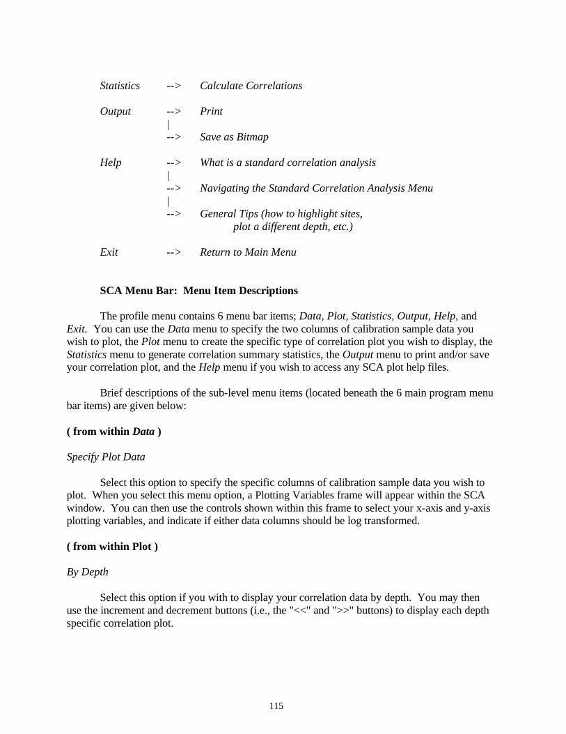
115

Statistics --> Calculate Correlations Output --> Print | --> Save as Bitmap Help --> What is a standard correlation analysis | --> Navigating the Standard Correlation Analysis Menu | --> General Tips (how to highlight sites, plot a different depth, etc.) Exit --> Return to Main Menu SCA Menu Bar: Menu Item Descriptions The profile menu contains 6 menu bar items; Data, Plot, Statistics, Output, Help, and Exit. You can use the Data menu to specify the two columns of calibration sample data you wish to plot, the Plot menu to create the specific type of correlation plot you wish to display, the Statistics menu to generate correlation summary statistics, the Output menu to print and/or save your correlation plot, and the Help menu if you wish to access any SCA plot help files. Brief descriptions of the sub-level menu items (located beneath the 6 main program menu bar items) are given below: ( from within Data ) Specify Plot Data Select this option to specify the specific columns of calibration sample data you wish to plot. When you select this menu option, a Plotting Variables frame will appear within the SCA window. You can then use the controls shown within this frame to select your x-axis and y-axis plotting variables, and indicate if either data columns should be log transformed. ( from within Plot ) By Depth Select this option if you with to display your correlation data by depth. You may then use the increment and decrement buttons (i.e., the "<<" and ">>" buttons) to display each depth specific correlation plot.

116

All depths simultaneously Select this option if you wish to create a single correlation plot which displays the calibration data associated with all of the sampling depths simultaneously. Bulk average only Select this option if you wish to just create a correlation plot of the bulk average calibration data (i.e., the average values across all sampling depths for each sample site). ( from within Statistics ) Calculate Correlations Select this menu option to create and display the basic correlation statistics associated with the two currently displayed data columns. These statistics will include the simultaneous, bulk average, and by depth correlation estimates (corresponding to the three types of correlation plots mentioned above). ( from within Output) Print Select this option to print the currently displayed correlation data plot. Save as Bitmap Select this option to save the currently displayed correlation data plot as a bitmap file. ( from within Help ) What is a standard correlation analysis Select this option to display the Standard Correlation Analysis help file, which explains what a standard correlation plot is and how it can be interpreted. Navigating the Standard Correlation Analysis Menu Select this option to display the Navigating the Standard Correlation Analysis Menu help file. This help file explains how to use the SCA menu commands to create, display, print and/or save correlation plots.

117

General Tips (how to highlight sites, plot a different depth, etc.) Select this option to display the General Tips help file. This help file explains how you can use the various interactive plotting features associated with most ESAP-Calibrate graphical displays, such as highlighting sites, plotting different sample depths, etc. ( from within Exit ) Return to Main Menu Select this option to close down the SCA window and return to the ESAP-Calibrate main menu. 5.7.3 Practice Module (Performing a Standard Correlation Analysis) In this practice session you will learn how to perform a standard correlation analysis using the Training2 demonstration calibration sample data (i.e., the sk13_lab97.pro profile data file). If you have not already done so, you should import the sk13_lab97.pro file now, before continuing on with this session (refer to practice module 5.2.3 if you've forgotten how to do this). After the Training2 profile data file has been imported, click on the Calibrate > Stochastic Methods > Standard Correlation Analysis main menu option. This will invoke and display the Standard Correlation Analysis window. Once this window displays, click on the Data > Specify Plot Data sub-menu option. A variable selection frame will then appear; you can use the controls within this frame to select your x-axis and y-axis data. For this practice session, select “boron” for the x-axis, “ECe” for the y-axis, and then click on the OK command button. Now click on the Plot > All Depths Simultaneously sub-menu option; a plot like the one shown in figure 5.4 should then appear. This plot displays the overall correlation structure between your boron and ECe sample data. If you wish to examine this relationship on a depth-by-depth basic, click on the Plot > By Depth sub-menu option. If you wish to study just the bulk average relationship, click on the Plot > Bulk Average Only sub-menu option. To calculate and display the correlation estimates for all of the above mentioned plots, click on the Statistics > Calculate Correlations option. To gain more experience, you should try creating these various plots and statistics now. In general, a standard correlation analysis can be performed on any two columns of data present in your profile data file. However, this analysis is most commonly used to examine the correlation structure between soil salinity (ECe) and other primary profile data columns (such as texture or water content). With this in mind, you might now wish to examine the correlation structure between 1) ECe and SP, 2) ECe and volumetric H2O, and 3) ECe and %H2O|FC. In particular, note that the bulk average correlation estimates between salinity and water content are quite high (0.784 and 0.845 for the volumetric H2O and %H2O|FC correlations, respectively. Figure 5.5 displays the bulk average ECe versus the bulk average %H2O|FC data. Recall that the 1D salinity profile plot from this field indicated that nearly all of the salinity profile

118

Figure 5.4 Overall correlation structure between boron and ECe sample data in sk13_lab97.pro data file. shapes were either uniform or inverted, and most of the salinity levels were also quite high. This current salinity / water content correlation plot indicates that the percent water content (relative to field capacity) increases as the bulk average salinity increases. In the absence of an established crop, this information strongly suggests that the elevated salinity conditions in this field are due (at least in part) to insufficient drainage.

Figure 5.5 Bulk average ECe v.s. %H2O|FC correlation structure within the sk13_lab97.pro data.

119

5.8 Performing a DPPC Correlation Analysis This section describes how to perform a DPPC correlation analysis on a DPPC type profile data file. The following material is covered in detail: (1) a description of the DPPC model, (2) the DPPC - PDCA (Profile Data Correlation Analysis) window, (3) the DPPC Graphics menu, and (4) guidelines for understanding how to interpret the DPPC - PDCA summary report and data plots. 5.8.1 What is a DPPC Profile Data Correlation Analysis A DPPC (Dual Pathway Parallel Conductance) correlation analysis represents the third type of stochastic data analysis method available in the ESAP-Calibrate program. A DPPC correlation analysis can be performed on any valid DPPC profile data file, either before or after merging such a profile data file with any corresponding survey data. This analysis allows you to calculate (i.e., estimate) a set of soil conductivity readings, based on your input sample salinity, texture, and water content data values. These calculated soil conductivity readings can then be compared to the input soil data, and/or your measured (i.e., true) conductivity readings (such as your input EM-38 readings, etc.). If you use the ESAP-Calibrate program much, you will soon find that a DPPC correlation analysis represents a very powerful analytical procedure. We recommend reading the two examples described below to develop a better understanding of how this procedure can be used to clarify the inter-relationships between your profile (soil sample) and conductivity (survey) data. Example #1: Suppose that your calibration sample data contains measurements of (1) salinity, (2) texture, (3) water content, (4) boron, and (5) nitrate, and that all this profile data has been acquired from a previous grid sampling survey. Also, suppose that no conductivity survey data has been acquired, and that your primary project goal is to determine the feasibility of measuring and mapping salinity, boron, and nitrate levels from an (as yet to be performed) conductivity survey. In this example, you should import your calibration sample data as a DPPC profile data set and then perform a standard DPPC profile correlation analysis (a standard analysis represents an analysis performed independently of any conductivity survey data). The DPPC procedure will automatically estimate a column of calculated conductivity readings and then add these calculated readings back into your profile data file. In practice, bulk average calculated conductivity estimates and true conductivity readings tend to be highly correlated (typical correlation values in actual survey applications usually exceed 0.9). Therefor, the DPPC procedure will substitute the calculated conductivity data (ECac) for the missing true survey data and then compute the correlation between the ECac data and each column of soil sample data. You can then examine these correlation values to obtain an approximate idea of how beneficial an actual conductivity survey would be in this field (i.e., just how strong should the correlation

120

be between your acquired conductivity data and salinity, boron, and/or nitrate sample data). In turn, you would use this information to appraise the feasibility of performing a conductivity survey. Example #2: Suppose that your sample profile data contains (1) salinity, (2) texture, (3) water content, and (4) bulk density, and that this profile data has been acquired from an ESAP generated sampling plan. Additionally, assume that EM-38 horizontal and vertical conductivity survey data has also been acquired at all your profile sites. Hence, your main project goal in this scenario is to determine the correlation(s) between the measured conductivity (ECa: which in this case is your EM-38 signal data), calculated conductivity (ECac), and soil salinity (ECe), and to determine the degree of "ECa / ECe signal deterioration" due to spatial variation in the soil texture, water content, and bulk density data. In this example, you should import your sample data as a DPPC profile data set, import your EM-38 survey data as a pre-saved *.svy file, and then perform a composite DPPC profile correlation analysis (a composite analysis represents an DPPC correlation analysis performed in conjunction with conductivity survey data). The DPPC procedure will again automatically estimate a column of calculated conductivity readings (i.e., ECac readings) and then add these calculated readings back into your profile data file. Next, the procedure will calculate all of the cross correlation estimates (between ECa, ECac, and ECe), and also compute the percentage of signal deterioration between the ECac and ECe readings, by depth, due to spatial variation in the secondary soil variables. For example, if the correlation between the ECa and ECac data is high, but the correlation between the ECa (or ECac) and ECe data is rather poor, then you should check the signal deterioration estimates. If these estimates are also high (i.e., > than 15%), then the poor ECa / ECe correlation is probably due to excessive spatial variation in the texture, water content, and/or bulk density data, etc. The above two examples represent only a brief introduction to the types of information available to you when you perform a DPPC data correlation analysis. You should refer to the rest of section 5.8 to gain a more thorough understanding of this analysis procedure, as well as the types of inference which can be drawn from it. 5.8.2 Description of the DPPC Model The DPPC (Dual Pathway Parallel Conductance) Model is an electrical conductance model developed by Rhoades (Rhoades et al., 1989) which described the relationship between bulk soil electrical conductivity (ECa), volumetric water content (Tw), and the electrical conductivity of the soil water (ECw). Mathematically, this model can be written as: (Ts+Tws)2 ECws(ECs) ECa = --------------------------------- + Twc(ECwc) [5.1] Ts(ECws) + Tws(ECs)

121

where Tws = volumetric water content in the soil-water pathway Twc = volumetric water content in the continuous liquid pathway Ts = volumetric content of the solid phase of the soil ECws = electrical conductivity of the soil-water pathway ECwc = electrical conductivity of the continuous liquid pathway ECs = electrical conductivity of the solid soil particles Additionally, if we define Tw = Tws + Twc = total volumetric water content ECw = average electrical conductivity of the soil-water, and assume that under equilibrium: ECw = ECws = ECwc then the above specified model can be written as: (Ts+Tws)2 ECw(ECs) ECa = --------------------------------- + (Tw-Tws)(ECw) [5.2] Ts(ECw) + Tws(ECs) Now, it is possible to either measure or estimate all the parameters on the right hand side of equation (5.2), provided that measurements of the soil ECe, SP, gravimetric water content (pW), and bulk density (Bd) are acquired. These relationships, as shown in Rhoades et al., 1989, are as follows: Tw = (pW)(Bd)/100 Tws = 0.639(Tw) + 0.011 Ts = Bd/2.65 ECs = 0.019(SP) - 0.434 ECw = [ (ECe)(Bd)(SP) / 100(Tw) ]. Additionally, note that when bulk density measurements are not available, the bulk density can be estimated from the SP measurements as follows: Bd = 1.73 - 0.0067(SP). Hence, it is possible to estimate the ECa given knowledge of the ECe, SP, pW, and (optionally) Bd. Such estimates are typically referred to as "calculated ECa" (or ECac) data values. Equation (5.2) shows how the inner-relationships between the salinity (ECe), soil texture (SP & Bd), and soil water content (pW) influence the measurement of bulk soil electrical

122

conductivity (ECa). When the variation in soil salinity across the survey area is significant, then equation (5.2) tends to be dominated by the ECe values. However, when the salinity variation is minimal, other soil properties can significantly influence the conductivity readings. Among other things, equation (5.2) demonstrates why conductivity survey information can often be used in non-saline areas to accurately map soil texture, water content, and/or other physical soil properties. If the soil salinity levels across the survey exceed about 1.5 dS/m, then equation (5.2) can be further simplified to: (Ts+Tws)2 (ECs) ECa = ------------------------ + (Tw-Tws)(ECw) [5.3] Ts since the product Ts(ECw) tends to be significantly larger than the product Tws(ECs), and thus the latter term can be ignored. Equation (5.3) is often referred to as the "linear version" of the DPPC model, since it expresses the relationship between conductivity (ECa) and salinity (ECe) in a linear manner. A complete description of the theoretical development of the DPPC equation can be found in the following technical article: Rhoades, J.D., N.A. Manteghi, P.J. Shouse, and W.J. Alves. 1989. Soil electrical conductivity

and soil salinity: new formulations and calibrations. Soil Sci. Soc. Am. J. 53: 433-439. Additionally, a good review article concerning the practical application of the DPPC equation for soil salinity estimation is: Rhoades, J.D. 1992. Instrumental field methods of salinity appraisal. pp. 231-248. In G.C. Topp et al. (ed.) Advances in measurements of soil physical properties: bringing theory into practice. SSSA Spec. Publ. 30. SSSA, Madison, WI. 5.8.3 Using the DPPC - PDCA Window All analysis routines associated with a Dual Pathway Parallel Conductance Profile Data Correlation Analysis can be accessed from the DPPC - PDCA window, which may be invoked and displayed by clicking on the Calibrate > Stochastic Methods > DPPC Correlation Analysis main menu option. These routines include (1) merging your conductivity survey and profile data files, (2) log transforming the calculated ECac, ECe, and/or any other input profile data columns, (3) displaying the DPPC correlation summary report and/or graphics window, and (4) saving the DPPC profile data correlation analysis summary report as an ASCII text file. Each of these analysis options are described below in more detail.

123

File Merge Options: The options contained within this frame can be used to merge your profile and survey data files together, provided that you have already imported a *.svy survey data file when you invoke the DPPC - PDCA window. You should first check the Merge active Survey / Profile Data File information check box if you wish to merge your survey and profile data files together. After you highlight this check box, the Merge Data command button will appear. Click on this button to merge your survey and profile data files together. After clicking on this command, the ESAP-Calibrate program will merge your two data files and display the View Log File command button. Next, click on this button to display and view a detailed description of the file merging results. In general, you should always view this log file to verify that the survey and profile data files were merged successfully. DPPC Analysis Options: The command buttons contained within this frame should be used to perform the actual DPPC profile data correlation analysis, and to display the analysis results. If desired, you can log transform one or more of your profile data columns before you perform the DPPC correlation analysis. You can also have the ESAP-Calibrate program log transform the calculated column of ECac data, before computing any correlation statistics. Log transformations may be specified by clicking on the Log Transform Columns command button. This will invoke and display the Log Transform Columns Window, which in turn can be used to specify the columns of data to log transform. In general, we recommend that you log transform the salinity (ECe) and calculated conductivity (ECac) data columns. You may also wish to log transform any profile data which is highly correlated with salinity, such as SAR, boron, various cation levels, etc. Log transforming such data usually results in more accurate and meaningful correlation estimates. Important: all log transformations requested using the Log Transform Columns option discussed above are TEMPORARY transformations only. As soon as the DPPC correlation estimates have been calculated, all log transformed columns are back-transformed into their raw data units, INCLUDING the calculated column of ECac data. After requesting any desired log transforms, you can click on the Perform DPPC Analysis command button to invoke the DPPC profile data correlation algorithm. When the algorithm finishes, the View Correlation Output and Plot Data command buttons will appear. You can click on the View Correlation Output button to display the DPPC profile data correlation analysis summary report. If desired, you may print this report using the print command option(s) associated with your default text editor. Additionally, you should click on the Plot Data command button if you wish to invoke and display the DPPC Graph Options window. You may then use the options associated with this window to produce various types of DPPC panel graphs.

124

File Save Options: The command buttons contained within the Save Results to ASCII Text File frame may be used to save the information contained within the DPPC summary report to a permanent ASCII text file. You should use the Specify Output Filename command button to specify the name of your permanent, output ASCII text file, and then the Save File button to save the ASCII text file. You should click on the Finished command button when you are done viewing and/or displaying your DPPC profile data correlation results. Note that before the DPPC - PDCA Window disappears, you will be asked if you would like to add the calculated column of ECac data into your active profile data file. Answer "yes" if you would like to be able to analyze this ECac data using any of the other ESAP-Calibrate stochastic data analysis methods, otherwise answer "no". 5.8.4 Understanding the DPPC Summary Report The DPPC-PDCA summary report contains all of the results from the complete correlation analysis, displayed in an easy to read table-like format. A standard summary report will contain the following 4 sub-sections: I. ECac Correlation Structure II. Bulk average ECac v.s. bulk average Primary / Secondary soil variable Correlations III. Bulk average and depth specific ECac v.s. depth specific Primary / Secondary soil variable Correlations IV. ECe - ECac Signal Deterioration: by depth A composite summary report will contain the 4 sub-sections listed above, along with a 5th sub-section entitled: V. Bulk average & depth specific Primary / Secondary soil variables v.s. z1-signal Correlations The output associated with each of these sub-sections is described in detail below. I. ECac Correlation Structure This section displays the correlation estimates between the depth specific and bulk average calculated conductivity (ECac) data. In the example shown below, the correlations between the log transformed bulk average ECac and the ECac associated with the 0.15 and 1.05 meter sample depths are 0.351 and 0.912, respectively.

125

Additionally, if you are performing a composite analysis, then this section will also display the correlations between the calculated (ECac) and measured (z1-signal) conductivity readings. (If you acquire 2 conductivity readings at each survey site, then the z1-signal data will represent an average of these 2 readings.) In the example shown below, the z1-signal data is highly correlated with the bulk average ln(ECac) data, r = 0.945, as well as the ln(ECac) data from the 0.45 and 0.75 sampling depths; r = 0.944 and 0.915, respectively. I. ln(Calc ECa) Correlation Structure and ln(Calc ECa) v.s. z1-signal Correlation Structure depth specific ln(Calc ECa) sample depth levels 0.15 0.45 0.75 1.05 ave ave ln(Calc ECa) 0.351 0.891 0.956 0.912 1.000 z1-signal data 0.351 0.944 0.915 0.788 0.945

II. Bulk average ECac v.s. bulk average Primary / Secondary soil variable Correlations This section displays the pair-wise correlations between the bulk average ECac and bulk average soil profile data columns. Note that all pair-wise correlations are displayed using a standard correlation matrix format. In the example shown below, the ln(ECac) / ln(ECe) correlation estimate is 0.864, the ln(ECac) / SP correlation estimate is 0.551, and the ln(ECe) / SP estimate is 0.084. II. Bulk ave ln(Calc ECa) v.s. bulk ave Pri/Sec Soil Variable Correlations Column Labels: 0. ln(Calc ECa) 1. ln(ECe) 2. SP 3. Vol H2o 4. Bulk Den 0 1 2 3 4 0 1.000 0.864 0.551 0.593 -0.377 1 0.864 1.000 0.084 0.132 0.043 2 0.551 0.084 1.000 0.920 -0.896 3 0.593 0.132 0.920 1.000 -0.824 4 -0.377 0.043 -0.896 -0.824 1.000

126

III. Bulk average and depth specific ECac v.s. depth specific Primary / Secondary soil variable Correlations This section displays the correlations between the depth specific soil profile data versus both the bulk average and depth specific ECac data. In general, depth specific profile data will correlate better with depth specific ECac readings, as opposed to the bulk average ECac readings. The differences between these two sets of correlation estimates represent the degree of improvement in the prediction accuracies you would achieve if you could acquire depth specific conductivity data (as opposed to conductivity data averaged across the entire soil profile). Example correlations for salinity (ln(ECe)) and texture (SP) are shown below. In particular, note that the prediction of the SP data in the 0.0-0.3 m sample depth could be greatly improved using depth-specific conductivity information (i.e., the correlation jumps from 0.267 to 0.948). III. Bulk ave & depth specific ln(Calc ECa) v.s. depth specific Pri/Sec Soil Variable Correlations Pri/Sec bulk depth Soil depth ave specific Variable level ln(Calc ECa) ln(Calc ECa) ln(ECe) 0.15 0.503 0.745 0.45 0.675 0.787 0.75 0.836 0.878 1.05 0.817 0.893 SP 0.15 0.267 0.948 0.45 0.612 0.602 0.75 0.643 0.641 1.05 0.403 0.423

. . . IV. ECe - ECac Signal Deterioration: by depth This section displays the calculated ECe - ECac signal deterioration, by depth, due to spatial variation in the remaining primary soil variables (i.e., texture, water content, and bulk density -- if measured bulk density data is available). ESAP calculates the signal deterioration as a percentage (from 0 to 100), where 0% represents no deterioration and 100% represents complete deterioration. In general, calculated values over 15% indicate moderate signal deterioration, and values over 25% represent serious deterioration. Typically, if the sample levels of the remaining primary soil variables are fairly constant across your survey area, then the signal deterioration will be minimal. On the other hand, if these data values are highly variable (and poorly correlated with the soil salinity levels), then the signal deterioration can be extreme. In the example shown below, the signal deterioration in the 0.15 and 0.45 sampling depths is severe (44.6% and 40.8%, respectively).

127

IV. ECe <-> Calc ECa Signal Deterioration: by depth depth % Signal level Deterioration 0.15 44.6 0.45 40.8 0.75 22.6 1.05 19.8 ave 26.2

V. Bulk average & depth specific Primary / Secondary soil variables v.s. z1-signal Correlations This final section will only be displayed if you are performing a composite DPPC analysis (i.e., if you have merged your conductivity survey and soil profile data together). This section displays the correlations between your z1-signal (conductivity) data and each of the depth specific and bulk average soil profile variables. In the example shown below, the z1-signal data appears to be fairly well correlated with the log salinity measurements from the 0.45, 0.75, and1.05 sample depths (0.742, 0.770, and 0.714) as well as the bulk average measurement data (0.801). However, the correlations between the z1-signal data and remaining soil variables range from marginal to poor. V. Bulk ave & depth specific Pri/Sec Soil Variables v.s. z1-signal Correlations Pri/Sec Soil Variable sample depth levels 0.15 0.45 0.75 1.05 ave ln(ECe) 0.476 0.742 0.770 0.714 0.801 SP 0.273 0.574 0.592 0.293 0.498 Vol H2o 0.114 0.641 0.565 0.421 0.595 Bulk Den -0.382 -0.236 -0.211 -0.269 -0.352

Note: The correlations shown in section V above actually represent "worst-case" scenarios for this survey / sample data set. In general, an estimated regression model can produce a better correlation between the conductivity and calibration sample data due to the inclusion of (1) both conductivity signal readings (rather than just a single average value), and (2) additional trend surface parameters, when such parameters are found to improve the prediction accuracy.

128

5.8.5 DPPC Data Plots After performing a DPPC profile data correlation analysis, you will have the option to view the results using one or more types of panel graphs. In the ESAP-Calibrate program, a panel graph is a series of 4 simultaneously displayed plots, where each plot displays the same y-axis variable against 4 different x-axis variables. In the DPPC panel graphs, the y-axis variable is always the calculated conductivity (ECac). Likewise, one or more soil profile variables will always be shown along the x-axis; however, the choice of which soil profile variable(s) to display is left to the user. The purpose of the panel graph is to show how the ECac calculations correlate with and/or are influenced by the displayed x-axis soil variables. All DPPC panel graphs can be created using the controls associated with the DPPC Graph Options window. This Graph Options window can be invoked by clicking on the Plot Data command button located within the main DPPC Profile Data Correlation Analysis window (note: this command button will only become visible after the DPPC correlation analysis has been performed). You should use the DPPC Graph Options window to specify the type of DPPC graph you wish to create and display. You can select from three different types of panel graphs: a standard panel, or one of two custom panel graph types. If you select a standard panel graph, then you do not need to enter any additional plotting information. However, if you select one of the two custom panel graph options, then you will need to specify additional plotting information, as described below. Standard Panel: Select this option if you wish to display the calculated ECa against the measured ECe, texture, volumetric water content, and bulk density, by sampling depth. This is referred to as a standard panel plot because these are the four soil variables which are used to determine the soil ECa levels. If you did not acquire bulk density data, then estimated bulk density levels (calculated from the soil texture levels) will be displayed in panel 4. Custom Panel 1 (Calc ECa v.s. 4 Secondary Variables): Select this option if you wish to display the calculated ECa against four user selected secondary soil variables, by sampling depth. If you choose this option, then a second plot input information frame will appear within the Graph Options Window. You should use the list boxes displayed within this frame to select the four secondary variables you wish to plot the ECa against. You may also use the controls contained within this frame to indicate if either the calculated ECa or any/all of the secondary soil variables should be log transformed. Custom Panel 2 (Ave Calc ECa v.s. depth specific Secondary Variable): Select this option if you wish to display the calculated bulk average ECa against a single secondary soil variable across multiple sampling depths (up to 4 depths may be displayed simultaneously). If you choose this option, then a second input information frame will appear

129

within the Graph Options window. You should use the list box displayed within this frame to select the secondary variable you wish to plot the ECa against. You should also use the controls contained within this frame to indicate if either the calculated ECa or the secondary soil variable should be log transformed, as well as to specify the secondary variable sampling depths you wish to display. Note that this last type of panel plot can be used to determine if the calculated bulk average ECa correlates well to depth specific soil variable information, such as depth specific soil ECe data, etc. 5.8.6 Navigating the DPPC Graphics Menu DPPC Graphics Menu Bar: Layout The ESAP-Calibrate DPPC Graphics menu bar is located in the upper left corner of the DPPC Graphics program window. The full layout for this menu bar system is shown below. Main level Sub-Level 2 Sub-Level 3 Output --> Print Current Graph(s) | --> Save as Bitmap | --> Save 1st Plot --> Save 2nd Plot --> Save 3rd Plot --> Save 4th Plot Help --> Navigating the DPPC Graphics Menu | --> General Tips (how to highlight sites, plot a different depth, etc.) Exit --> Return to DPPC Graph Options Menu

130

DPPC Graphics Menu Bar: Menu Item Descriptions The profile menu contains 3 menu bar items; Output, Help, and Exit. You can use Output menu to print and/or save your panel plot(s), and the Help menu if you wish to access any DPPC Graphic help files. Brief descriptions of the sub-level menu items (located beneath the 3 main program menu bar items) are given below: ( from within Output) Print Select this option to print the currently displayed panel plots. (Note: all displayed panel plots will be automatically printed on the same page of printer paper.) Save as Bitmap Select this option to save any one of the currently displayed panel plots as a bitmap file. You should specify which plot you wish to save using the following layout guidelines; 1st plot = upper left hand plot, 2nd plot = upper right hand plot, 3rd plot = lower left hand plot, 4th plot = lower right hand plot. ( from within Help ) Navigating the DPPC Graphics Menu Select this option to display the DPPC Graphics Menu help file. This help file explains how to use the DPPC Graphics menu commands to print and/or save panel plots. General Tips (how to highlight sites, plot a different depth, etc.) Select this option to display the General Tips help file. This help file explains how you can use the various interactive plotting features associated with most ESAP-Calibrate graphical displays, such as highlighting sites, plotting different sample depths, etc. ( from within Exit ) Return to DPPC Graph Options Menu Select this option to close down the DPPC Graphics Window and return to the DPPC Graph Options Window. If desired, you can select a new (i.e., different) panel plot to display using the options associated with this latter window.

131

5.8.7 Practice Module (Performing a DPPC Correlation Analysis) Section 5.8.4 describes in detail the correct way to interpret the results from a DPPC correlation print-out. To recreate the output data shown in that section, you should import both the survey and profile data files associated with the Training1 project (i.e., the b102data.svy and bwd_102lab.pro data files). Once you have imported the Training1 data files, click on the Calibrate > Stochastic Methods > DPPC Correlation Analysis menu option to invoke and display the DPPC-PDCA window. After this window displays, check the “Merge active Survey / Profile data file” check box, and then click once on the Merge Data command button (you just merged the *.svy and *.pro data file information together). Next, click on the Log Transform Columns command button, check the “Calc ECa” and “ECe” check boxes, and then click on the OK command button (this indicates that you would like to log transform these two data columns). Now click on the Perform DPPC Analysis command button (to perform the analysis) and then the View Correlation Output command button to display the results. These results should match the results shown in section 5.8.4. If you wish to create any DPPC data plots, click on the Plot Data command button. This will invoke and display the DPPC Graph Options window; the controls within this window can then be used to select your graph type. The panel graphs shown in figure 5.6 below show a standard panel for the 0.15 meter depth; i.e., the relationships between the calculated ln(ECa) and the measured ln(ECe), SP, volumetric H2o, and bulk density for the 0.0-0.3 meter samples. Note that you can view the data for each sample depth (and/or the bulk average data) by simply clicking on the Increment / Decrement command buttons.

132

Figure 5.6 Standard panel graph for the 0.15 meter profile data from the bwd_102lab.pro data file. Note that the calculated ECa appears

to be more correlated with the measured SP texture data than the measured salinity data.

133

5.9 Spatial Regression Modeling (Stochastic Calibration) This section describes how to estimate, validate, and use a stochastic calibration model to predict the values of a response variable (such a soil salinity) from soil conductivity information. There are many stochastic calibration model selection and validation techniques available for use in the ESAP-Calibrate program. Although most of these techniques are covered in detail in this section, some of these represent advanced procedures which the beginning user may wish to skip over at first. (Note: all sub-sections covering advanced material are clearly identified.) 5.9.1 What is a Stochastic Calibration Model In the ESAP-Calibrate program, a stochastic calibration model is a spatially referenced, multiple linear regression model. Typically, such a regression model would include both conductivity and trend surface parameters. For example, suppose that we wish to predict the log soil salinity levels within a field from log transformed EM38 conductivity survey readings acquired across the field. Then we might wish to use the following regression model: ln(ECe) = b0 + b1[ln(EMh)] + b2[ln(EMv)] + b3[x] + b4[y] [5.4] where EMh and EMv represent the EM-38 survey readings, and x and y represent the spatial coordinate locations of the EM-38 survey data. Hence, the purpose of the regression fitting procedure would be to optimally estimate the regression parameters; i.e., to estimate the values of b0, b1, b2, b3, and b4. Once the parameter estimates were acquired, we could then predict the log salinity levels at every survey site, as well as estimate the accuracy associated with any or all of these site predictions. The regression equation shown above represents only one hypothetical example. In practice, transformed and decorrelated signal data (i.e., the principal component scores) are often used in place of the raw signal readings as predictor variables in the regression equation. Additionally, different fields may require different numbers of signal or trend surface parameters, and even if the form of the regression equation is the same for two different fields, the actual parameter estimates typically will not be. Variation in the model parameter estimates should be expected; this variation arises naturally due to changing survey conditions (i.e., due to differences between fields in soil temperature, texture, water content, crop cover, bed-furrow shape, etc.). In particular, the stochastic calibration modeling procedures contained within the ESAP-Calibrate program are designed to help you (1) determine the best regression model parameter form, and (2) optimally estimate these model parameters. Once this regression model has been estimated, you can then use the stochastic calibration prediction procedures to predict the levels of your soil variable across the entire field (or survey area), estimate the average field level, and calculate a number of additional, useful prediction statistics. You can also generate and save an output file of your predictions, which can then be imported into the ESAP-SaltMapper program and used to generate a spatial prediction map. Furthermore, all of the modeling and prediction techniques described above can be used to generate predictions of your soil variable across multiple sampling depths, provided you acquire multiple depth calibration sample data.

134

5.9.2 Navigating the SCM Menu SCM Menu Bar: Layout The ESAP-Calibrate SCM menu bar is located in the upper left corner of the SCM program window. This window can be invoked and displayed by clicking on the Calibrate > Stochastic Methods > Spatial MLR Analysis main menu option. The full layout for this menu bar system is shown below. Main level Sub-Level 2 Sub-Level 3 Model --> Select Response Variable | --> Identify Model Parameters | --> Estimate Calibration Equation | --> Advanced Options | --> View model summary | statistics --> View residual summary | diagnostics --> View residual plots Predict --> View prediction plots | --> Calculate field summary statistics | --> Save output predictions Test --> Calculate Net-Flux tests Help --> What is a stochastic calibration model | --> What information is provided by the | Advanced modeling options | --> Navigating the SCM Menu | --> Frequently Asked SCM Questions Exit --> Return to Main Menu

135

SCM Menu Bar: Menu Item Descriptions The profile menu contains 5 menu bar items; Model, Predict, Test, Help, and Exit. You can use the Model menu options to identify, estimate, and if desired, appraise your stochastic calibration model, the Predict menu options to view prediction plots, calculate field summary statistics, and create and save your output predictions, the Test menu option to perform Net Flux tests, and the Help menu if you wish to access any SCM help files. Brief descriptions of the sub-level menu items (located beneath the 5 main program menu bar items) are given below: ( from within Model ) Select Response Variable Select this option to identify your stochastic calibration model response variable (i.e., the soil variable you wish to predict). When you select this option ESAP will display the Response Variable Specification window, which can in turn be used to (1) merge your survey and profile data files together, (2) identify your response variable, and (3) create preliminary plots of the response variable versus the conductivity instrument readings. Identify Model Parameters Select this option to identify the form of your stochastic calibration (regression) equation. When you select this option ESAP will display the MLR Model Identification window, which can be used to either manually or automatically identify an optimal regression equation. Estimate Calibration Equation When you select this option ESAP will display the MLR Model Estimation window, which you can use to estimate your specified stochastic calibration (regression) equation. Advanced Options At any time after ESAP estimates a regression equation, you can access a full set of model and residual error diagnostics using the sub-menu items located under the Advanced Options menu option. The information which can be displayed includes a complete set of model summary statistics, residual error summary diagnostics, and a full range of graphical residual plots. (Note: if you do not have any prior regression modeling experience, you do not need to access any of these sub-menu options.)

136

( from within Predict ) View prediction plots Select this option to view the accuracy of the stochastic calibration (regression) model predictions. When you select this option ESAP will display the 2D Prediction Scatter Plot window, which you can use to create plots of the observed (true) versus model predicted soil variable data. Calculate field summary statistics Select this option to calculate your field summary statistics. When you select this option ESAP will display the Field Summary Statistics window, which you can use to produce summary statistics for your survey area. These summary statistics include the field mean (or median) predictions, survey area interval estimates, and when estimating soil salinity, the expected relative crop yield loss (for a specific crop type) due to the current salinity condition. Save output predictions You should select this option to save your regression model predictions as an ESAP output *.prd data file. By design, any *.prd output file can be automatically imported into the ESAP-SaltMapper program and used to construct spatial prediction maps of the soil variable(s) you have modeled. ( from within Test ) Calculate Net-Flux tests Select this option to display the Net Flux Calculation window. If you acquire additional soil samples in the future at some (or all) of your calibration sites within your survey area, you can use these new samples to statistically determine if the average magnitude of the predicted soil variable has changed over time. Such tests are commonly referred to as "net-flux" tests, and these tests can be performed using the options available within the Net Flux Calculation window. ( from within Help ) What is a stochastic calibration model Select this option if you would like to display the help file which briefly describes what a stochastic calibration model is, and how such a model is commonly used for prediction purposes.

137

What information is provided by the Advanced modeling options Select this option if you would like to display the help file which briefly describes some of the summary and graphical display features associated with the ESAP-Calibrate advanced modeling options. Navigating the SCM Menu Select this option to display the SCM Menu help file. This help file explains how to use the SCM menu commands to invoke and/or preform all of the various modeling and prediction procedures associated with the stochastic calibration modeling component of the ESAP-Calibrate program. Frequently Asked SCM Questions This is the help documentation you should read if you need more detailed information about how to use the various SCM procedures. For example, you should refer to this file for specific information about specifying and estimating a regression model, calculating various summary statistics and model predictions, or using the net flux testing procedure, etc. ( from within Exit ) Return to Main Menu Select this option to close down the SCM Window and return to the Main program window. 5.9.3 Response Variable Specification Window You should use the Response Variable Specification window to select the profile variable that you wish to predict (i.e., use as the response variable) in you stochastic calibration model. This window can be invoked and displayed by clicking on the Model > Select Response Variable SCM menu option. There are three steps you must perform when you display this window: (1) set the active project directory, (2) select the appropriate response variable, and (3) merge the survey and profile data files. You should verify that your two data files were merged correctly. If desired, you can also create and view some preliminary response variable data plots and/or delete one or more profile data sites. To estimate a stochastic calibration model, you first need to merge your active survey and profile files together into a single calibration data file. If these two files are stored in different project directories, then you can choose which project directory to save your regression modeling output results to using the Survey Project or Profile Project option buttons listed in the Set Active Project Directory frame. (Note: if your survey and profile projects directories are one in the

138

same, then it does not matter which directory you select.) Next, you should use the list box shown in the Select Response Variable frame to select the appropriate response variable for your calibration model. If desired, you can also log transform this variable by highlighting the log transform check box shown to the immediate right of the list box. Finally, you should click on the Merge Data command button once you are ready to merge your survey and profile data files together. Once these two files have been processed, a File Merge Results frame will appear which displays the merging results (i.e., which sampling designs your profile data associates with). If the displayed results appear to be in error, then you should click on the View Log File command button to display a detailed summary of the file merging results. Otherwise, you can accept the merging results by simply clicking on the Accept Results command button, unless you wish to use one of the additional features described below. (Note: once you click on the Accept Results, Reject Results, or Cancel command buttons, the Response Variable Specification window will disappear and the Stochastic Calibration Modeling window will be displayed, allowing you to once again access the main stochastic calibration modeling menu items.) Plot Data: Click on this command button if you would like to create and view any preliminary response variable (PRV) plots. This will invoke the PRV window, which you may then use to produce either (1) bi-variate response variable plots, or (2) plots of the response variable against the primary (z1) principal component score. (These plots are explained in more detail in section 5.9.4, which describes the PRV graphics menu layout and features.) Delete a Site: The Site Deletion window is invoked and displayed when you click on the Delete a Site command button. The options within this window can be used to remove (i.e., delete) the profile data core associated with a specific sample site from the current calibration data file. You should invoke the Site Deletion window ONLY if you wish to remove a profile data core from your current calibration sample data file BEFORE estimating the regression model. In general, you should not use this feature unless you have already tried to model the current response variable and discovered one or more extreme outliers which must be removed from the calibration sample data. To delete a site, select the appropriate sample site number from the displayed sample site list box and then click on the "Delete this Site" command button. Note that you can only delete one site at a time, i.e., you can not highlight and delete multiple sites at once. (If you wish to delete more than one site, you will need to interactively re-invoke this Site Deletion window from within the Response Variable Specification window.)

139

5.9.4 Navigating the Preliminary Response Variable (PRV) Graphics Menu PRV Graphics Menu Bar: Layout The ESAP-Calibrate PRV Graphics menu bar is located in the upper left corner of the PRV window. The full layout for this menu bar system is shown below. Main level Sub-Level 2 Plot --> Response Variable v.s. z1 | (primary decorrelated signal data) | --> Bivariate response variable plots Output --> Print | --> Save as Bitmap Help --> Navigating the PRV Graphics Menu | --> General Tips (how to highlight sites, plot a different depth, etc.) Exit --> Return to Response Variable Specification Window PRV Graphics Menu Bar: Menu Item Descriptions The profile menu contains 4 menu bar items; Plot, Output, Help, and Exit. You can use the Plot menu to select the type of plots to create and display, the Output menu to print and/or save your plot(s), and the Help menu if you wish to access any PRV Graphic help files. Brief descriptions of the sub-level menu items (located beneath the 4 main program menu bar items) are given below: ( from within Plot ) Response variable v.s. z1 (primary decorrelated signal data) Select this option to create and display plots of your selected response variable against the primary (z1) principal component score, by depth. These plots are useful for determining if your response variable data responds to your conductivity signal data in a linear manner, and also for determining the strength of correlation between the response variable and the conductivity readings. (Note: recall that when you have collected two signal readings at each site, the z1 component simply represents an average of these two readings.)

140

Bivariate response variable plots Select this option to create and display a series of bivariate plots of your response variable across different sampling depths. These plots are useful for determining the vertical correlation structure inherent in your response variable data. (Note: if your sample profile data was collected from only a single sampling depth, then this plotting option will not be available.) ( from within Output) Print Select this option to print the currently displayed plot. Save as Bitmap Select this option to save the currently displayed plot as a bitmap file. ( from within Help ) Navigating the PRV Graphics Menu Select this option to display the PRV Graphics Menu help file. This help file explains how to use the PRV Graphics menu commands to create, display, print and/or save PRV plots. General Tips (how to highlight sights, plot a different depth, etc.) Select this option to display the General Tips help file. This help file explains how you can use the various interactive plotting features associated with most ESAP-Calibrate graphical displays, such as highlighting sites, plotting different sample depths, etc. (Note: sites displayed in PRV plots can not be highlighted.) ( from within Exit ) Return to Response Variable Specification Window Select this option to close down the PRV Graphics Window and return the Response Variable Specification Window. 5.9.5 Specifying the Calibration Model Parameters In order to estimate a stochastic calibration model, you must specify the model parameters from within the MLR Model Identification window. This window can be invoked and displayed by clicking on the Model > Identify Model Parameters SCM menu option. The model parameters can be specified one of four ways: you can let ESAP choose a default standard model, you can manually select a standard model, you can manually define and specify a custom

141

model, or you can have ESAP auto-select an appropriate model. Your calibration model parameters will typically consist of two components; signal parameters and trend surface parameters. All signal parameters are incorporated using the principal component scores; keep in mind that these principal component scores simply represent linear combinations of your (possibly log transformed) survey signal data columns. In a similar manner, all trend surface parameters are incorporated using centered and scaled (x,y) coordinate data, where the (x,y) coordinates are adjusted to lie between the bounds of 0 < x <1 and 0 < y < 1, respectively. These scaling techniques help insure that the matrix inversion techniques used by the regression modeling algorithm remain stable. In general, the goal of the model identification process is to identify which signal parameters and which (if any) trend surface parameters should be incorporated into the final calibration model. If you are unfamiliar with general regression modeling techniques, then you should let ESAP decide the optimal parameter combination. However, if you have training and/or experience fitting statistical regression models, then we recommend that you use standard modeling diagnostic techniques to determine an appropriate parameter combination for your particular data set. To determine the parameter combination, highlight one of the appropriate model identification methods shown in the Model Identification Method frame; this should correspond to the identification method you wish to employ for selecting the model calibration parameters. You may choose from any one of the three methods listed below. Auto-Select an Appropriate Model: You should select this option if you would like ESAP to automatically examine a number of possible parameter combinations, and then select the parameter combination which generates the lowest cumulative PRESS score. In regression modeling, a PRESS score represents the sum of squares of the "jack-knifed" prediction errors, and low PRESS scores generally indicate more accurate models. (Jack-knifing is a technique where each data point is temporarily removed from the data set, the model is estimated using the remaining data points, and then the predicted value at the removed site is compared to the true value. The prediction errors, which represent the difference between the predicted and true values, are then squared and summed together to create the PRESS score.) Manually Select a Standard Model: This is the default model identification method. You may be able to choose from up to 12 different parameter combinations, depending on your profile data calibration sample size and the number of signal readings you collected at each site (i.e., either 1 or 2). If you have no prior experience fitting regression models, we recommend that you use this identification method, and simply accept the default selection that ESAP generates when the MLR Model Identification window is first displayed.

142

Define and Specify a Custom Model: You should select this option if you wish to specify a custom (i.e., non standard) parameter combination. This option may allow you to choose from up to 36 different parameter combinations, depending on your profile data calibration sample size and the number of signal readings you collected at each site. Once you have selected an appropriate parameter combination, click on the OK command button to return to the SCM window. 5.9.6 Understanding the Model Parameter Specification Options The ESAP-Calibrate program uses a set of standard abbreviations to indicate the various regression model parameter combinations you may choose from. In order to use the advanced features of the model identification options, you need to understand what these abbreviations mean. The definitions shown below may be used as a reference for these abbreviations. Definitions: Raw Signal Readings: s1 and s2 (note: s1 and s2 may be log transformed) Decorrelated Signal readings: z1 and z2 Relationship: z1 = a1(s1 - mean[s1]) + a2(s2 - mean[s2]) z2 = a3(s1 - mean[s1]) - a4(s2 - mean[s2]) where a1, a2, a3, and a4 are determined by the principal components algorithm If only one signal reading has been collected at each site, then z1 = a1(s1 - mean[s1]), where a1 = 1 / (std.dev[s1]). Raw Location Coordinates: u and v Scaled Location Coordinates: x and y Relationship: x = (u - min[u]) / k y = (v - min[v]) / k where k = the greater of (max[u] - min[u]) or (max[v] - min[v])

143

Abbreviations: Signal parameters are shown using the abbreviations z1, z2, or z12 (i.e., z1 squared, where z12 = z1*z1). Trend surface parameters are shown as x, y, xy (xy = x*y), x2 (x2 = x*x), and y2 (y2 = y*y). Additionally, 1st OT is an abbreviation for "first order trend surface" (i.e., the parameters x and y), and 2nd OT is an abbreviation for "second order trend surface" (i.e., the parameters x, y, xy, x2, and y2). Various numbers of signal and trend surface parameters can be mixed together to form the final model parameter combination. The combinations shown below represent a few of the possible standard and custom model definitions. Abbreviation Corresponding Regression Model z1 b0 + b1(z1) z1 + 1st OT b0 + b1(z1) + b2(x) + b3(y) z1, x, y same as above z1 + 2nd OT b0 + b1(z1) + b2(x) + b3(y) + b4(xy) + b5(x

2) + b6(y2)

z1, x, y, xy, x2, y2 same as above z1, z2 b0 + b1(z1) + b2(z2) z1, z12 b0 + b1(z1) + b2(z12) z1, z2, z12, x, y, y2 b0 + b1(z1) + b2(z2) + b3(z12) + b4(x) + b5(y) + b6(y

2) Restrictions: All calibration models must contain an intercept term, as well as a z1 signal parameter. No parameter combination can be specified if the number of parameters (including the intercept) is greater than the number of sample sites minus 2: i.e., # of parameters <= # of samples - 2. Additionally, no z2 signal term can be specified if only one signal reading was acquired at each sample site, nor can any higher order terms be entered into a model without also including the corresponding lower order term (for example, x2 can not be included without first including x, etc.). Advanced Options (associated with the 3 Model Identification Methods) Standard Model frame: Up to 12 different parameter combinations can be manually selected using the option buttons displayed in the Standard Model frame. The ESAP generated default standard parameter combinations are as follows:

144

# of signal # of calibration default parameter readings per site sample sites combination 1 <= 6 z1 1 > 6 z1, x, y (z1 + 1st OT) 2 <= 7 z1, z2 2 > 7 z1, z2, x, y ( [z1,z2] + 1st OT) These default selections usually generate reasonable calibration models. However, you are free to choose any parameter combination associated with an active standard model option button. Custom Model frame: The Custom Model Definition frame will be displayed if you select the custom model identification method. This frame contains two sub-frames. You should use the option buttons displayed in the Signal Parameters sub-frame to select an appropriate combination of signal parameters. Likewise, you can use the option buttons displayed in the Trend Surface Parameters sub-frame to select a specific combination of trend surface parameters. Your final model will then contain both sets of selected parameters (i.e., signal + trend). Note that if you have acquired 2 signal readings per site, and you have collected samples from at least 11 calibration sites, then you can potentially create a total of 36 separate regression model parameter combinations. Automatic Model Identification frame: The Automatic Model Identification frame will be displayed if you request the auto-selection model identification method. The options within this frame may be used to control the types of parameter combinations which are analyzed, as well as to invoke the auto-selection procedure and display the results. Analysis Options (Unrestricted v.s. Restricted): Before you invoke the auto-selection algorithm, you have the option of restricting the possible parameters to specific parameter combination subsets. For example, you can request that ESAP only consider standard types of parameter combinations, or only models without any trend surface parameters, etc. Analyze All Possible Models: Select this option if you wish ESAP to analyze all possible parameter combinations (this is the default).

145

Eliminate All Models Which Use x-Location Trend Surface Components: Select this option if you wish to eliminate all models which use any x location trend surface components. Eliminate All Models Which Use y-Location Trend Surface Components: Select this option if you wish to eliminate all models which use any y location trend surface components. Eliminate All Models Which Use 2nd Order Trend Surface Components: Select this option if you wish to eliminate all models which use either quadratic (x2, y2) or interaction (xy) trend surface components. Eliminate All Models Which Use Any Trend Surface Components: Select this option if you wish to eliminate all models which use any trend surface components. Eliminate All Non-Standard Type Models: Select this option if you wish to limit the analysis to only those parameter combinations displayed in the Standard Model frame. Click on the Invoke Auto-Selection Algorithm command button when you are ready to invoke the auto-selection algorithm. Note that this algorithm may take some time to process all the various models (possible up to a few minutes in some cases). Once the auto-selection algorithm has finished, you can click on the View Results command button to view a tabular listing of all the PRESS score results. These results will include the value of the minimum PRESS score, each models relative PRESS score ratio (i.e., that models PRESS score divided by the minimum PRESS score), and the ranking of each analyzed model with respect to the minimum PRESS score. After the auto-selection algorithm has finished, you can choose to either accept or reject the auto-selected model. Typically you should view the auto-selection results before making this decision. If you accept the selection, ESAP will record the parameter combination which produced the minimum PRESS score, close down the MLR Model Identification window, and then return to the Stochastic Calibration Modeling window. If you reject this selection, then the Automatic Model Identification frame will disappear, but the Model Identification window will still remain active. You will then need to select a different parameter combination using one of the other model identification options.

146

5.9.7 Estimating the Calibration Model You should invoke the MLR Model Estimation window once you are ready to estimate your stochastic calibration equation (i.e., after you have selected your response variable and identified your model parameters). This window can be invoked and displayed by clicking on the Model > Estimate Calibration Equation SCM menu option. After you invoke this window, the currently selected calibration model structure will be displayed. Two additional model / residual estimation options can be invoked before estimating your calibration equation. First, you can request that your calibration equation be fit to the bulk average response variable values, in addition to each set of depth specific values. (Note: if your calibration samples come from only one sampling depth, then this option will be disabled.) This option is useful when you wish to automatically create estimates of bulk average response data (such as the average salinity levels throughout the profile). Second, you can calculate Moran Residual Spatial Autocorrelation (MRSA) test statistics for each calibration equation. These residual diagnostic test statistics can be used to help determine if the model residuals are spatially independent. By default, ESAP will not generate these test statistics. In general, we recommend that you only request these test statistics if you understand how they work. After you have checked any desired options, click on the Estimate command button to initiate the calibration model estimation algorithm. When the estimation process is complete, the MLR Model Estimation window will disappear and the basic calibration model summary statistics will be written to the lower left hand corner of the SCM program window. 5.9.8 Practice Module 1 (Specifying and Estimating a Salinity Calibration Equation) In this practice session you will learn how to estimate a salinity calibration equation using the Training2 demonstration data (i.e., the sk13data.svy survey and sk13_lab97.pro profile data files). The results from this exercise will also be used in the next practice module (section 5.9.13; Practice Module 2). If you have not already done so, you should import both files now, before continuing on with this session. After the Training2 data files have been imported, click on the Calibrate > Stochastic Methods > Spatial MLR Analysis main menu option. This will invoke and display the Stochastic Calibration Modeling (SCM) window. To estimate your salinity calibration equation, you must perform the three sequential steps listed below: Step 1: Select the response variable Step 2: Identify the regression model parameters Step 3: Estimate the equation

147

To perform the first step, click on the Model > Select Response Variable SCM menu option. This will invoke and display the Response Variable Specification window. Now select “ECe” from the drop-down response variable list, check the “log transform” check box, and click on the Merge Data command button. Verify that the file merge results appear correct (in this example you should see 15 sample sites associated with the User Specified SD label), and then click on the Accept Results command button. You have just selected your response variable (i.e., log transformed salinity), and you should see this response variable information appear on the SCM window (within the Response Variable Information frame). To perform the second step, click on the Model > Identify Model Parameters SCM menu option. This will invoke and display the MLR Model Identification window. When this window appears, highlight the “Auto-select an appropriate model” option, click on the Invoke Auto-Selection Algorithm, and then relax for a few moments while the ESAP-Calibrate program performs the model optimization process. Once this process is finished, click on the Yes command button within the Accept Selection frame. You have now just used the ESAP-Calibrate program to auto-select an appropriate set of regression model parameters, and you should now see this information also appear on the SCM window (the selected model should be: ln(ECe) = b0 + b1(z1) + b2(z2)). To perform the third step, click on the Model > Estimate Calibration Equation SCM menu option. This will invoke and display the MLR Model Estimation window. When this window appears, check the “Fit this model to the bulk average sample values” check-box, and then click on the Estimate command button. The ESAP-Calibrate program will then estimate a regression model for each sample depth, and inform you when the estimation process is finished. After you click on the message box OK command button, the Estimation window will disappear and some basic model summary statistics will appear within the Model Summary Statistics frame on the SCM window. If you have followed the above directions correctly, your summary statistics should be identical to the statistics shown below. Depth R-square Est-CV 0.15 0.9025 23.850% 0.45 0.8828 26.822% 0.75 0.8585 23.841% 1.05 0.7969 22.344% bulk ave 0.9263 17.101% Note that the R-square column reflects the regression model fitted R2 values, and the Est-CV column reflects the estimated model coefficient of variation (CV) values on the back-transformed data. (If you had not log transformed the salinity data, then the second column would have instead shown the regression model root mean square error estimates.)

148

5.9.9 Viewing 2D Prediction Scatter Plots Once the calibration equation has been estimated, you can view 2D scatter plots of the observed versus predicted response data. These plots give you a convenient way to judge the adequacy of your calibration equation, in addition to the basic model summary statistics automatically displayed in the SCM program window. Two plot types are available for viewing: an ordinary prediction plot and a jack-knifed prediction plot. An ordinary observed versus predicted plot shows the correlation between the actual (i.e., true) versus regression predicted data values. An observed versus jack-knifed predicted plot shows the correlation between the true data against the jack-knifed predicted data, where the jack-knifed estimates are calculated by interactively removing each data point from the regression model, re-calculating the model, and then using the re-calculated model to predict the removed point. You should use the 2D Prediction Scatter Plot Initialization window to initialize the specific type of prediction scatter plot you wish to display, and to control which sub-sets of predictions are displayed. This window can be invoked and displayed from the 2D Prediction Scatter Plot program window, which can in turn be invoked by clicking on the Predict > View Prediction Plots SCM menu option. Directions for navigating the 2D Prediction Scatter Plot menu are given below. 2D Prediction Scatter Plot Menu Bar: Layout The ESAP-Calibrate 2D Prediction Scatter Plot menu bar is located in the upper left corner of the 2D Prediction Scatter Plot program window. The full layout for this menu bar system is shown below. Main level Sub-Level 2 Sub-Level 3 Plot --> Specify New Plot Variables | --> Create Plot Output --> Print --> Obs vs Prd | --> Obs vs JK-Prd | --> Both Plots | --> Save as Bitmap | --> Obs vs Prd

--> Obs vs JK-Prd

Help --> Navigating the 2D Prediction Scatter Plot Menu | --> General Tips (how to plot a different depth)

149

Exit --> Return to the SCM Menu 2D Prediction Scatter Plot Menu Bar: Menu Item Descriptions The 2D prediction scatter plot menu contains 4 menu bar items; Plot, Output, Help, and Exit. You can use the Plot menu to initialize and create different types of prediction scatter plots, the Output menu to print and/or save these plots, and the Help menu if you wish to access any 2D prediction scatter plot help files. Brief descriptions of the sub-level menu items (located beneath the 4 main program menu bar items) are given below: ( from within Plot ) Specify New Plot Variables Select this menu option to invoke and display the 2D Prediction Scatter Plot Initialization window, which you can then use to initialize your specific scatter plot. Create Plot Select this menu option to create and display the most recently initialized scatter plot. ( from within Output) Print Select the sub-options listed under this menu item to print the most recently displayed observed versus predicted and/or jack-knife predicted scatter plots. Save as Bitmap Select the sub-options listed under this menu item to save the most recently displayed observed versus predicted and/or jack-knife predicted scatter plots as a bitmap file. ( from within Help ) Navigating the 2D Prediction Scatter Plot Menu Select this option to display the Navigating the 2D Prediction Scatter Plot Menu help file. This help file explains how to use the menu commands to create, display, print and/or save the various types of 2D prediction scatter plots.

150

General Tips (how to plot a different depth) Select this option to display the General Tips help file. This help file explains how you can use the various interactive plotting features associated with most ESAP-Calibrate graphical displays, such as highlighting sites, plotting different sample depths, etc. ( from within Exit ) Return to the SCM Menu Select this option to close down the 2D Prediction Scatter Plot Window and return to the SCM (Stochastic Calibration Modeling) menu. 5.9.10 Calculating Field Summary Statistics The Calculate Field Summary Statistics window can be used to request the calculations of the mean survey area predictions and survey area interval estimates. This window can be invoked and displayed by clicking on the Predict > Calculate Field Summary Statistics SCM menu option. These statistics are used to summerize the survey process, and they must be calculated before an ESAP output prediction file (i.e., a *.prd file) can be created and saved. To effectively perform the summary statistic calculations, you will need to request the proper estimation options, as described below. Field Average Estimates: After estimating your calibration model, ESAP will compute the average level of these predictions across the entire survey area, on a depth specific basis. These averages are referred to as field average estimates. For example, if you have estimated a set of salinity calibration models for 4 sampling depths, ESAP will calculate the field average estimate associated with each depth. If your calibration model is based on log transformed response data, then all calculated field average estimates will be automatically reported on a log scale. You should highlight the Back Transform Mean Field Log Predictions check box if you wish to back-transform these log average estimates into field median estimates. Range Interval Cut-off Levels: In addition to calculating average level predictions, ESAP can also calculate what percentage of your survey area falls within specific range intervals. In other words, if you have estimated a soil salinity calibration model, you can request ESAP to calculate the proportion of your survey area with soil salinity levels falling between certain threshold values. You should use the option controls located within the Range Interval Cut-off Levels frame to specify both

151

the number of cut-off levels and the value of each cut-off level. For example, if you wanted to define four salinity intervals as < 2, 2-4, 4-8, and > 8 dS/m, you would select 3 cut-off levels and enter 2, 4, and 8 into the 1st, 2nd, and 3rd input text box, respectively. If your calibration model is based on log transformed response data, but your cut-off levels have been entered using non-transformed units, then you should highlight the Log Transform cut-off levels check box. Note that by highlighting this check box, you are telling ESAP to log transform your input cut-off levels. If desired, you can also have the ESAP-Calibrate program automatically set the cut-off levels for you using a Salinity Lab salt tolerance threshold-slope equation. To do this, click on the Set Levels (using salt-tolerance curves) command button. This action will invoke and display the Salt Tolerance window, which is explained in detail in section 5.9.11. However, this Set Levels command button will only be visible if you request 4 cut-off levels, and that this feature should only be used if you are calculating soil salinity predictions. Statistical Calculations: After defining all of the calculation options, click on the Calculate Statistics command button. The ESAP-Calibrate program will then calculate the mean survey area predictions and survey area interval estimates, and display the View Output command button. Click on this latter command button to view the ASCII output text file which contains your field summary statistics; i.e., the text file which contains all of the mean survey area predictions and survey area interval estimates. If you wish to save the current ASCII output text file as a permanent text file, highlight the Yes option under the Save Results to ASCII Text File frame and use the Specify Output File Name and Save File command buttons to name and save the file, respectively. You should click on the Specify Output File Name command button to display the File Open window, which you can then use to specify a permanent output file name. Likewise, click on the Save File button to save your file. After the file has been saved, a message box will be displayed confirming the location of your permanent text file. 5.9.11 Using the Salt Tolerance Window The Salt Tolerance window, which can only be invoked from the Calculate Field Summary Statistics window, should be used to set the soil salinity range interval cut-off levels corresponding to an appropriate salt tolerance equation. These cut-off levels are determined by the ESAP-Calibrate program from the salt tolerance equation you select, and in turn allow the ESAP program to estimate the relative yield loss occurring in your field. You should first indicate which conductivity units your soil salinity samples are measured in by highlighting either the dS/m or mS/m Salinity unit options. Next, you should use the options shown in the Salt Tolerance frame to select or define the specific salt tolerance equation.

152

You can select from a number of different crop types by using the Crop Type list box. The selected crop type will in turn define the salt tolerance parameters (i.e., the threshold and % slope estimates). Or if desired, you can enter your own (custom) threshold and slope parameter estimates. To do this, select "custom" for your crop type and then type in your parameter estimates directly into the threshold and slope input text boxes. Be sure to enter the threshold value in the correct units, and note that the slope estimate is expressed as the % reduction in yield given a 1 unit increase in ECe. After you have specified the crop type, you need to indicate the type of depth integration weights you would like to use in the yield loss calculations. These weights can be thought of as root distribution weights, sense they allow you to specify which sampling depths should have the greatest effect on the crop yield. For example, suppose you have sampled down to 4 feet in 1 foot intervals, and the field crop is cotton. Then you might use a linear weighting scheme (0.4, 0.3, 0.2, 0.1) to indicate that the salinity levels in the 1st foot should account for 40% of the overall yield loss calculations, since you expect 40% of the root distribution to lie within the 1st foot of topsoil, etc. The Salt Tolerance window supplies two standard depth integration weighting options; Equal weighting and Linear weighting. Additionally, you can highlight the User Defined Weighting option if you wish to specify your own set of depth integration weights. Once you highlight this option, a series of input weight text boxes will appear; you should type your weight values directly into these text boxes. Please note that all values must be greater than or equal to 0, and these weight values must sum to 1. Once you have finished initializing the various salt tolerance and depth weighting options discussed above, click on the OK command button to return to the Calculate Field Summary Statistics window. After you request the summary calculations, your ASCII output text file should contain an estimated "relative yield loss" value (in addition to the standard field average and range interval estimates). This latter value represents the projected yield loss incurred due to the current soil salinity pattern, as compared to the yield one would expect under ideal (i.e., non-saline) conditions. 5.9.12 Saving your Output Predictions You can save your output prediction data at any point after you have calculated the field summary statistics. To create a permanent *.prd prediction data file, simply click on the Predict >Save Output Predictions SCM menu option. This action will invoke and display a File Save window, which can then be used to name and save your output file. Note that you must create a permanent ESAP-Calibrate prediction data file if you wish to use the ESAP-SaltMapper program to create any prediction transect plots or raster maps. In general, we recommend that you always create such a file.

153

5.9.13 Practice Module 2 (Analyzing, Summarizing, and Saving Prediction Data) In this last practice session you will learn how to analyze, summarize, and save regression based salinity prediction data. This session will make use of the output from Practice Module 1 (section 5.9.8). If you have not already done so, you should you should complete Practice Module 1 now. Once your calibration equation (i.e., regression model) has been estimated, you can proceed to analyze and summarize your output prediction data. This should be done by viewing the prediction plots and calculating the field summary statistics. To invoke and display the 2D Prediction Scatter Plot window, click on the Predict > View Prediction Plots SCM menu option. After this window appears, click on the Plot > Specify New Plot Variables sub-menu option. After the Plot Initialization window appears, highlight the “All Depths Simultaneously” option, check the “Back-Transform Data” check-box, and then click on the Initialize Plot command button. (You have just instructed the ESAP-Calibrate program to plot all the sample depths together, and to back-transform the observed and predicted ln(ECe) data values.) Now click on the Plot > Create Plot sub-menu option; the prediction plot which appears should look like figure 5.7 shown below. (Note: the title will not appear unless you manually add it.)

Figure 5.7 Observed versus predicted Training2 salinity data. As suggested by the regression model summary statistics, this plot confirms that the fitted calibration equation can adequately predict the soil salinity levels from the acquired conductivity survey data. Hence, you can now proceed to calculate the field summary statistics.

154

To invoke and display the Field Summary Statistics window, click on the Predict > Calculate Field Summary Statistics SCM menu option. Once this window displays, you should perform the following steps. First, check the “Back-transform mean field log predictions...” check-box (this instructs the ESAP-Calibrate program to back-transform the average field log salinity estimates into median estimates). Next, click on the Set Levels command button. After a warning message displays, the Salt-Tolerance window will appear. Now select “sorghum” from the drop-down crop list, highlight the “linear weighting across depths” option, and then click on the OK command button. (You have now just set your range interval cut-off levels using the threshold-slope salt tolerance equation for sorghum. This in turn will allow the ESAP-Calibrate program to estimate the relative expected yield loss in this field, in addition to the field median salinity levels and range interval estimates.) Finally, click on the Calculate Statistics command button to perform the summary calculations. Once the calculations are finished, click on the View Output command button to view the summary statistics. The statistical output in your summary file should be identical to the output shown in table 5.2. In most situations, you should print out and save the generated summary statistics text file. This output file will contain all of the pertinent summary statistics for your survey area, including the predicted median salinity estimates, by depth, the range interval area estimates, and the expected relative crop loss (if requested). In this training example, the median ECe estimates all lie between 10.5 and 12.0 dS/m, and a sorghum crop grown under these predicted field salinity conditions would suffer an expected 53.5% yield loss. Once you are done viewing the summary statistics, you should save your output salinity predictions to a permanent ESAP *.prd prediction data file. To do this, click on the Predict > Save Output Predictions SCM menu option. When the Save Output Predictions window appears, click on the Specify Output File Name command button, type in your output file name (for example, ece_sk13.prd), click on the windows Open command button, and then the Save File command button. You should then see an ESAP-Calibrate message stating that your output file has been saved. If you desire, you can now leave the ESAP-Calibrate program, start up the ESAP-SaltMapper program, and create a 2D raster map of your predicted salinity data (the ESAP-SaltMapper program is described in detail in Chapter 3). An example map of the predicted bulk average salinity data created using the ESAP-SaltMapper program is shown in figure 5.8.

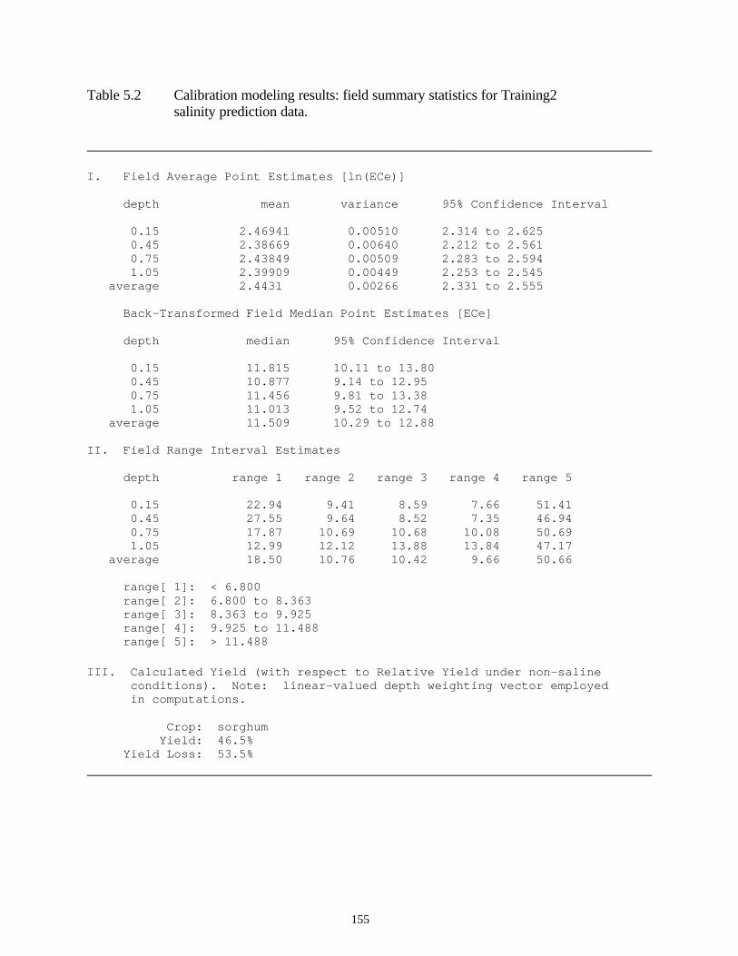
155

Table 5.2 Calibration modeling results: field summary statistics for Training2 salinity prediction data. ______________________________________________________________________________ I. Field Average Point Estimates [ln(ECe)] depth mean variance 95% Confidence Interval 0.15 2.46941 0.00510 2.314 to 2.625 0.45 2.38669 0.00640 2.212 to 2.561 0.75 2.43849 0.00509 2.283 to 2.594 1.05 2.39909 0.00449 2.253 to 2.545 average 2.4431 0.00266 2.331 to 2.555 Back-Transformed Field Median Point Estimates [ECe] depth median 95% Confidence Interval 0.15 11.815 10.11 to 13.80 0.45 10.877 9.14 to 12.95 0.75 11.456 9.81 to 13.38 1.05 11.013 9.52 to 12.74 average 11.509 10.29 to 12.88 II. Field Range Interval Estimates depth range 1 range 2 range 3 range 4 range 5 0.15 22.94 9.41 8.59 7.66 51.41 0.45 27.55 9.64 8.52 7.35 46.94 0.75 17.87 10.69 10.68 10.08 50.69 1.05 12.99 12.12 13.88 13.84 47.17 average 18.50 10.76 10.42 9.66 50.66 range[ 1]: < 6.800 range[ 2]: 6.800 to 8.363 range[ 3]: 8.363 to 9.925 range[ 4]: 9.925 to 11.488 range[ 5]: > 11.488

III. Calculated Yield (with respect to Relative Yield under non-saline

conditions). Note: linear-valued depth weighting vector employed in computations. Crop: sorghum Yield: 46.5% Yield Loss: 53.5%

______________________________________________________________________________

156

Figure 5.8 Final predicted bulk average ECe pattern, using Training2 salinity data (raster map created by the ESAP-SaltMapper program). 5.9.14 Advanced Options: Net Flux Testing The Net Flux window can be used to import and test for changes in the levels of calibration sample data collected across your survey area, if you collect additional sample data at one or more calibration sites in the future. This window can be invoked and displayed by clicking on the Test > Calculate Net Flux Tests SCM menu option. A net flux testing situation could arise as follows. Suppose you perform an electromagnetic survey on a salt affected field, select 12 survey locations for soil sampling, and then use the ESAP-Calibrate program to generate predicted salinity data. After examining the predicted salinity map, the farmer decides to leach the field by applying 2 acre feet of irrigation water for a 30 day period. After 30 days (i.e., after the leaching process), you re-enter this field,

157

re-sample the 12 calibration sites (acquiring 12 new soil cores), and determine the new soil salinity levels at these 12 sites. Then, by using the options in the Net Flux window, you can enter this data into the ESAP-Calibrate program and test whether or not the salinity pattern has changed (and if so, by how much). The above example focuses on soil salinity. However, the ESAP-Calibrate program can perform net flux tests on any soil variable you sample. The only requirement is that the locations of your new sample sites must coincide with your original calibration sites. Mathematically, it is possible to test for a change in a predicted soil variable over time provided that the monitoring site locations coincide with any of the original survey grid locations; for example, see Lesch et al., 1998, Monitoring for temporal changes in soil salinity using electromagnetic induction techniques., Soil Sci. Soc. of Am. J. 62:232-242. Future releases of the ESAP-95 software package will support this technique; however, version 2.01 currently does not support this testing methodology. Using the Net Flux window options You should use the options shown in the Data File Structure frame to define the number of monitoring sites contained in your monitoring data file, as well as the specific sampling depths. If desired, monitoring data files can contain less sample depths than the original calibration data, and/or not be present for every calibration site. However, it is required that your monitoring data file have the following column format: site_ID, depth 1, depth 2, ..., depth k where k represents the deepest monitoring depth, the columns of monitoring data are arranged in order from shallowest to deepest, and the site_ID column is the first column in the text file. The data for each monitoring site (i.e., each record) can be either space or comma delimitated. Note also that the ESAP-Calibrate program assumes that your input monitoring soil variable is the same as the currently active calibration variable in the MLR module. You should use the Specify Input File Name and Import Data command buttons located within the Data File Input frame to import your monitoring data file. Additionally, you can click on the View Log File command button if you would like to view a listing of the file merging results. (Note: you do not have to view this log file unless an error occurs during the file merging process.) Depending on the specific soil variable you are testing, one or more of the following testing options may be enabled. If necessary, these options can be invoked as described below: Log transform the input monitoring data values: If your response variable has been log transformed, you will be given the option of log transforming your input monitoring data. If you wish to apply such a log transformation, then highlight this log transform option.

158

Calculate a Net Flux test on the bulk average estimates: If you have estimated a bulk average stochastic calibration model, and you have imported monitoring data corresponding to each original calibration sample depth, then you will be given the option of testing for a bulk average change. If you wish to test for such a change, then highlight this bulk average option. Calculate Net Flux estimates for each monitoring site: If desired, you can have ESAP calculate net flux estimates for each monitoring site (on a depth by depth basis), in addition to the field average net flux calculation (which by default is always computed). You should highlight this option if you wish to have ESAP calculate these additional, individual net flux estimates. Once you have specified any of the applicable testing options described above, click on the Calculate Net Flux Test Results command button to calculate the requested net flux test statistics. Once the calculations are completed, you can use the View Test Results command button to view the calculated net flux test statistics. As with most other ESAP-Calibrate procedures, the command buttons contained within the Save Results to ASCII Text File frame may be used to save the net flux testing information to a permanent ASCII text file. You should use the Specify Output Filename command button to specify the name of your permanent, output ASCII text file, and then the Save File button to save the ASCII text file. 5.9.15 Advanced Options: Advanced Modeling Information If you are familiar with the statistical details behind regression modeling, you can use the ESAP-Calibrate program to access three different types of advanced model summary displays. Each of these displays are briefly described below. Advanced Model Summary Statistics If you wish to view any advanced regression model summary statistics, click on the Model > Advanced Modeling Options > View Model Summary Statistics SCM menu option. The ESAP-Calibrate program will then display an MLR Analysis and Statistics summary sheet which will include an analysis of variance (AOV) table and a listing of the parameter estimates for each estimation depth. This summary sheet will be displayed using your default text editor, and you will also have the option of saving this summary sheet as a permanent ASCII text file.

159

Advanced Residual Summary Diagnostics If you wish to view any advanced residual summary diagnostics, click on the Model > Advanced Modeling Options > View Residual Summary Diagnostics SCM menu option. The ESAP-Calibrate program will then display an MLR residual diagnostic summary sheet. This sheet displays univariate r-student residual summary statistics for each estimation depth, HAT leverage and r-student residual values for each depth, and the residual correlation matrix. If requested, the Moran residual spatial-correlation test statistics will also be shown at the bottom of this sheet. As before, this summary sheet will be displayed using your default text editor, and you will also have the option of saving this summary sheet as a permanent ASCII text file. Advanced Residual Plots In addition to the two summary sheets discussed above, the ESAP-Calibrate program can be used to produce a number of useful residual diagnostic plots. These plots can be used to graphically access the adequacy of the fitted regression model. If you are familiar with the use of various graphical residual diagnostic techniques, then you will find these plots to be very useful for model validation purposes. There are six types of diagnostic plots available for you to use, and each plot can be displayed using the Residual Diagnostics Plot window. To invoke and display this window, click on the Model > Advanced Modeling Options > View Residual Plots SCM menu option. This window contains its own set of help file documentation; you should read this documentation if you wish to learn more about interpreting the various residual diagnostic plots and/or how to navigate the Residual Diagnostics menu.

160

6.0 References Cook, P.G. and G.R. Walker. 1992. Depth profiles of electrical conductivity from linear combinations of electromagnetic induction measurements. Soil Sci. Soc. Am. J. 56:1015-1022. Diaz, L. and J. Herrero. 1992. Salinity estimates in irrigated soils using electromagnetic induction. Soil Sci. 154:151-157. Lesch, S.M., J.D. Rhoades, L.J. Lund, and D.L. Corwin. 1992. Mapping soil salinity using calibrated electromagnetic measurements. Soil Sci. Soc. Am. J. 56:540-548. Lesch, S.M., D.J. Strauss and J.D. Rhoades. 1995a. Spatial prediction of soil salinity using electromagnetic induction techniques: 1. Statistical prediction models: A comparison of multiple linear regression and cokriging. Water Resour. Res. 31:373-386. Lesch, S.M., D.J. Strauss and J.D. Rhoades. 1995b. Spatial prediction of soil salinity using electromagnetic induction techniques: 2. An efficient spatial sampling algorithm suitable for multiple linear regression model identification and estimation. Water Resour. Res. 31:3387-398. Lesch, S.M., J. Herrero and J.D. Rhoades. 1998. Monitoring for temporal changes

in soil salinity using electromagnetic induction techniques. Soil Sci. Soc. of Am. J. 62:232-242. McKenzie, R.C., W. Chomistek, and N.F. Clark. 1989. Conversion of electromagnetic inductance readings to saturated paste extract values in soils for different temperature, texture, and moisture conditions. Can. J. Soil Sci. 69:25-32. McNeil, J.D. 1980. Electromagnetic terrain conductivity measurement at low induction numbers. Tech. Note TN-6, Geonics Limited, Ontario, Canada. McNeil, J.D. 1986. Rapid, accurate mapping of soil salinity using electromagnetic ground conductivity meters. Tech. No. TN-18, Geonics Limited, Ontario, Canada. Rhoades, J.D. 1992. Instrumental field methods of salinity appraisal, pp. 231- 48, in Advances in measurement of soil physical properties: Bring theory into practice. G.C. Topp, W.D. Reynolds, and R.E. Green (Eds.). SSSA Special Publ. no.30. ASA, CSSA, and SSA, Madison, WI.

161

Rhoades, J.D. 1996. Salinity: electrical conductivity and total dissolved salts. In Methods of Soil Analysis, Part 3, Chemical Methods. Soil Sci. Soc. Am. Book Series 5, Am. Soc. of Agronomy, Inc. Madison, WI, pp. 417-435. Rhoades, J.D., N.A. Manteghi, P.J. Shouse, and W.J. Alves. 1989. Estimating soil salinity from saturated soil-paste electrical conductivity. Soil Sci. Soc. Am. J. 53:428-433. Rhoades, J.D. and D.L. Corwin. 1990. Soil electrical conductivity: effects of soil properties and application to soil salinity appraisal. Commun. Soil Sci. Plant Anal. 21:837-860. Rhoades, J.D., P.J. Shouse, W.J. Alves, N.A. Manteghi, and S.M. Lesch. 1990. Determining soil salinity from soil electrical conductivity using different models and estimates. Soil Sci. Soc. Am. J. 54:46-54. Rhoades, J.D., D.L. Corwin, and S.M. Lesch. 1991. Effect of soil ECa-depth profile pattern on electromagnetic induction measurements. Research Report #125, 108 p. Rhoades, J.D., F. Chanduvi, and S.M. Lesch. 1999. Soil salinity assessment: Methods and interpretation of electrical conductivity measurements. FAO Irrigation and Drainage Paper #57, Food and Agriculture Organization of the United Nations, Rome, Italy. Slavich, P.G. 1990. Determining ECa-depth profiles from electromagnetic induction measurements. Aust. J. Soil Res. 28:443-452. Weisberg, S. 1985. Applied linear regression. Second Ed. John Wiley & Sons, NY. Williams, B.G., and G.C. Baker. 1982. An electromagnetic induction technique for reconnaissance surveys of soil salinity hazards. Aust. J. Soil Res. 20:107-118. Yates, S.R., R. Zhang, P.J. Shouse, and M. Th. van Genuchten. 1993. Use of geostatistics in the description of salt-affected lands, pp. 283-304, in Water Flow and Solute Transport in Soils: Developments and Applications. Advanced Series in Agriculture, Series no. 20. D. Russo and G. Dagan (Eds.). Springer Verlag, NY.