Ernesto F. L. Amaral

Cohort mortality

Ernesto F. L. Amaral

September 19–26, 2019Demographic Methods (SOCI 320)

Cohort mortality• Cohort survival by analogy• Probabilities of dying• Columns of the cohort life table

– King Edward’s children

– From nLx to ex– The radix

• Annuities and insurance• Mortality of the 1300s and 2000s

2

Cohort survival by analogy• Analyze lifelines and the deaths that occur in the

diagonal stripe on the Lexis diagram that represents a particular cohort’s experience– Understand measures of survival and probabilities of

dying as a function of age for the cohort

• We could also analyze the rectangle on a Lexis diagram that represents some period– We would consider the lifelines that cross the rectangle

and the deaths that fall inside it

3

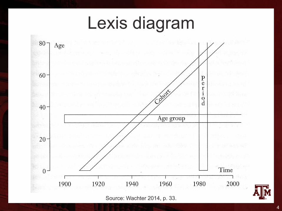
Lexis diagram

Source: Wachter 2014, p. 33.4

Why start with cohort measures?• The period measure is more complicated

– People at risk of dying at different ages are different people

• For the experience of a cohort over time– People at risk of dying at different ages are the same

people

• Cohort measures are conceptually simpler than period measures, so we begin with them

5

Disadvantage• Disadvantage of cohorts measures is being out of

date• To have complete measures of cohort mortality

for all ages, we have to wait until all members of the cohort have died– Rates for young ages refer to the distant past

• The most recent cohorts with complete mortality data are those born around 1900

• Measures of period mortality are more complicated, but they use more recent data

6

Basic cohort measures• The basic measures of cohort mortality are

elementary

– Take the model for exponential population growth

– Apply it to a closed population consisting of the members of a single cohort

– Change the symbols in the equations, but keep the equations themselves

7

Why is it a closed population?• If our population consists of a single cohort

– No one else enters the population after the cohort is born

– Babies born to cohort members belong to later cohorts, not to their parents’ cohort

– For this cohort, the only changes in population size come from deaths to members of the population

• Measures from chapter 1 reappear with new names in an analogy between populations and cohorts...

8

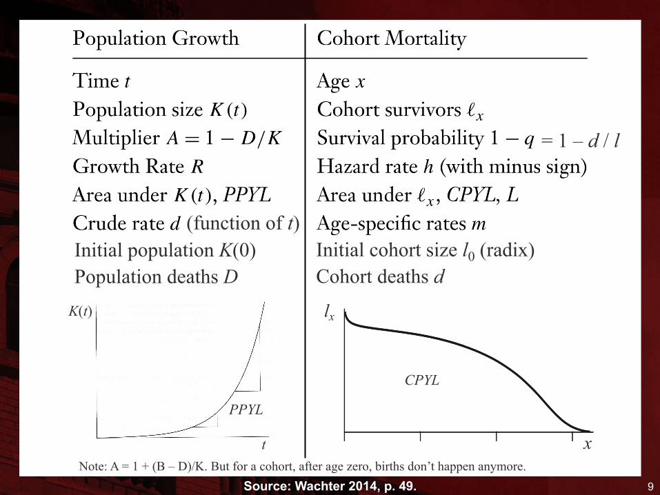
9Source: Wachter 2014, p. 49.

K(t)

t

PPYL

Initial population K(0)Population deaths D

Initial cohort size l0 (radix)Cohort deaths d

Note: A = 1 + (B – D)/K. But for a cohort, after age zero, births don’t happen anymore.

= 1 – d / l

(function of t)

lx

x

CPYL

Multiplication process• The same process of multiplication for population

growth happens for cohort mortality– It is not the mortality rates (m) that multiply

– It is not the probabilities of dying (q)

– It is the probabilities of surviving (1 – q)

• Age x is the subscript on the cohort survivors: lx– Time t is used for population size: K(t) = Kt

• The notation is different but the idea is the same

10

Multiplicative rules• Multiplicative rule for population growth

K(t + n) = A K(t)

• Multiplicative rule for cohort survivorshiplx+n = (1 − nqx) lx

– Subscript n specifies the length of the interval– nqx : probability of dying within an interval of length n

that starts at age x and ends at age x+n– lx+n : members who survive to age x+n

11

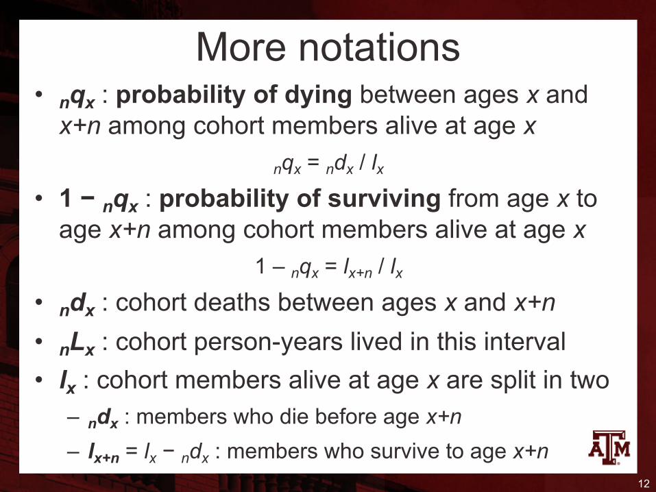
More notations• nqx : probability of dying between ages x and x+n among cohort members alive at age x

nqx = ndx / lx• 1 − nqx : probability of surviving from age x to

age x+n among cohort members alive at age x1 – nqx = lx+n / lx

• ndx : cohort deaths between ages x and x+n• nLx : cohort person-years lived in this interval• lx : cohort members alive at age x are split in two

– ndx : members who die before age x+n– lx+n = lx − ndx : members who survive to age x+n

12

Some more notations• In the expression nqx the left subscript gives the

width of the age interval and the right subscript gives the starting age

• 10q20 : probability of dying between 20 and 30– Not between 10 and 20– Do not confuse nqx with n multiplied by qx– If you want to multiply n by lx, use this notation: (n)(lx)

• 10q20 goes from 20.00000 to 29.99999– “The interval from 20 to 30” (including exact age 20,

excluding exact age 30)– Some authors call it “the interval from 20 to 29”

13

Example• A cohort born in 1984 reached age 18 in 2002

and 1,767,644 were alive at their 18th birthday

– Only 724 of them died before age 19

• Probability of dying

1q18 = 1d18 / l18 = 724 / 1,767,644 = 0.000410

• Probability of surviving

1 − 1q18 = 1 – 0.000410 = 0.999590

l19 / l18 = 1,766,920 / 1,767,644 = 0.999590

14

Hazard rates• Hazard rates can express the pace of death

within cohorts• Hazard rate is the counterpart of population

growth rate– We measure population growth with slopes of

logarithms of population size– We can measure cohort losses with slopes of

logarithms of numbers of survivors

• We insert a minus sign to make the hazard rate into a positive number– Because cohorts decrease as they age– i.e., cohorts grow smaller, not larger, as they age

15

Hazard rate formula• The hazard rate for a cohort is minus the slope of

the logarithm of the number of cohort survivors as a function of age

• Expressing hazard rate (hx) in the interval starting at age x (omitting any subscript for n)

• Formula for cohort survivorship resemble formula for exponential population growth

Kt+n = Kt eRn16

!"#$ = !" &'$() = !" &'()$

* = 1, !-.

/0#$/0ℎ" = −1, !-.

!"#$!"

Example• The cohort of boys born in the United States in

1980 started out with 1,853,616 members– 1,836,853 of them survived to their first birthday

17

ℎ" = − %& '()

*+,-*+

ℎ" = − %% '()

%,/01,/20%,/20,1%1

ℎ" = − '() 0.990957ℎ" = − −0.009084ℎ" = 0.009084

Probabilities of dying• A hazard rate is a rate like R, whereas nqx is a

probability• The word “probability” suggests a random

process• Randomness refers in principle to a randomly

selected member of our cohort• The occurrence of death appears partly random

and partly determined by causes – These causes are partly random and partly determined

by prior causes

19

nqx-conversions• Problems that involve working out nqx values for

different x and n are called “nqx-conversions”• Demographers frequently find themselves with

data for one set of age intervals when they need answers for different intervals– They may have data for 1-year-wide intervals and

need answers for 5-year-wide intervals

– They may have data for 15-year intervals and need answers for 5-year intervals

– They may have tables for ages 25 and 30 and need to know how many women survive to a mean age of childbearing of, for example, 27.89 years

20

Applying multiplication to lx• From our analogy with population growth, we go

from lx to lx+n by multiplication• We go from l65 to l85 by multiplying by 1 − 20q65

l85 = (1 − 20q65) l65• We go from l85 to l100 by multiplying by 1 − 15q85

l100 = (1 − 15q85) l85• We go from l65 to l100 by multiplying by the

product (1 − 20q65)(1 − 15q85)l100 = (1 − 20q65)(1 − 15q85) l65

21

Survival probabilities multiply• While we are interested in q, we work with 1 − q• We do not multiply the nqx values

– To die, you can die in the first year or in the second year or in the third year, and so on

– You only do it once– There is no multiplication

• We multiply the 1 − nqx values– To survive 10 years you must survive the first year and

survive the second year and survive the third year, and so on

– These “ands” mean multiplication

22

Basic assumption• We need an assumption when we do not have

direct data for short intervals of interest, such as 1-year-wide intervals

• We need an assumption when we only have data for wider intervals, such as 5-year-wide intervals

• We assume the probability of dying is constant within each interval where we have no further information

23

Applying assumption• If we do not know 1q20 or 1q21 but we do know 2q20

• We assume that the probability of dying is constant between ages 20 and 22

1q20 = 1q21 = q• Then (1 – q)2 has to equal 1 – 2q20

• More generally, for y between x and x+n–1(1 – 1qy)n = 1 – nqx

1 − 1qy = (1 – nqx)1/n

1qy = 1 − (1 − nqx)1/n

24

Example 1• For the cohort of U.S. women born in 1980

2q20 = 0.000837

• Calculate 1q20

1qy = 1 − (1 − nqx)1/n

1q20 = 1 − (1 − 2q20)1/2 = 1 – (1 – 0.000837)1/2

1q20 = 1 – (0.999163)1/2 = 1 – 0.999581

1q20 = 0.000419

25

Example 2• For the cohort of women born in 1780 in Sweden

5q20 = 0.032545

• Calculate 1q20

1qy = 1 − (1 − nqx)1/n

1q20 = 1 − (1 − 5q20)1/5 = 1 – (1 – 0.032545)1/5

1q20 = 1 – (0.967455)1/5 = 1 – 0.993405

1q20 = 0.006595

26

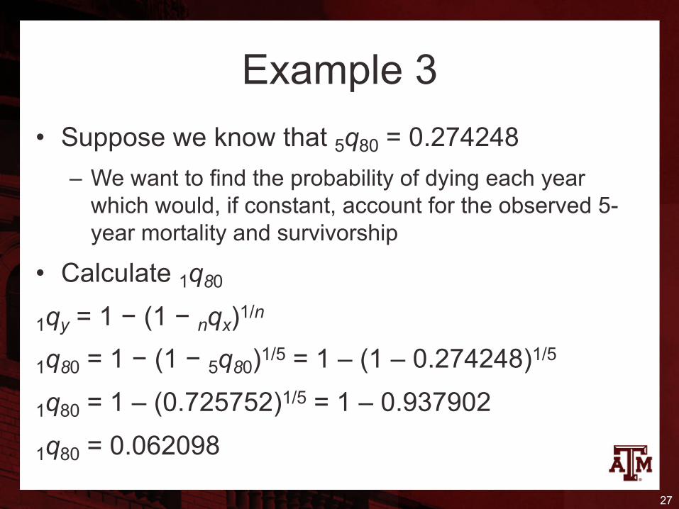
Example 3

• Suppose we know that 5q80 = 0.274248

– We want to find the probability of dying each year which would, if constant, account for the observed 5-year mortality and survivorship

• Calculate 1q80

1qy = 1 − (1 − nqx)1/n

1q80 = 1 − (1 − 5q80)1/5 = 1 – (1 – 0.274248)1/5

1q80 = 1 – (0.725752)1/5 = 1 – 0.937902

1q80 = 0.062098

27

Example 4• More elaborate conversion problems arise

• We might have values from a forecast of survival for the U.S. cohort of women born in 1980

l65 = 0.915449; l75 = 0.799403; 35q65 = 0.930201

• We might want the probability of surviving from 70 to 100: l100 / l70

!"##!$#

= 1 − 30*70 =!"##!,-!$#!,-

= 1 − 35*651 − 5*65 =

1 − 0.9302011 − 10*65 -/"# =

0.0697991 − 10*65 "/4 =

0.069799!$-/!,- "/4

!"##!$#

= 0.0697990.7994030.915449

"4= 0.069799

0.873236"4= 0.0697990.934471 = 0.074694

28

Use the Lexis diagram• The best way to solve complicated conversion

problems is to begin by drawing a diagonal line on a Lexis diagram– Mark off each age for which there is information about

survivorship at that age

– Mark off ages which are the endpoints of intervals over which there is information about mortality within the interval

– Between each marked age, assume a constant probability of dying, and apply the conversion formulas

29

Columns of the cohort life table• Lifetable is a table with lx and nqx as columns with

a set of other measures of mortality

• Columns and their names and symbols are fixed by tradition– This is customary since the 1600s– Each column is a function of age, so the columns of

the lifetable are sometimes called “lifetable functions”

• Rows correspond to age groups

31

Information in lifetable columns• All the main columns of the lifetable contain the

same information from a mathematical point of view– With some standard assumptions any column can be

computed from any other

• But they present information from different perspectives for use in different applications– Survivors

– Deaths– Average life remaining

32

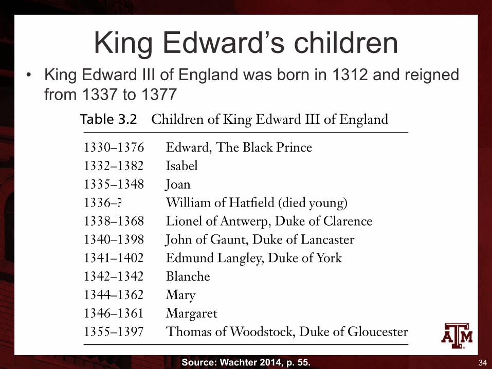
King Edward’s children• King Edward III of England was born in 1312 and reigned

from 1337 to 1377


Lexis diagram for King Edward’s children


Constructing a cohort life table• Generally, lifetables are constructed with 1-year

or 5-year intervals– A complete life table provides life table functions in

single years of age

– Lifetables in which functions are given for age groups are called “abridged lifetables” in older works

• Usually, for lifetables with 5-year-wide intervals– The first age group is a 1-year-wide interval (0–1)

– The second age group is a 4-year-wide interval (1–5)

36

Start of age group (x) and width (n)• Lifetables begin with a column labeled x

– Starting age for the age group

• The next column has the width n of the age group– The difference between the value of x for this row and

the value for the next age group found in the next row

• The last age group is called the “open-ended age interval” since it has no maximum age– Symbol for infinity (∞) is used for the length of this

interval

– We don’t set any upper limit of our own37

Number of survivors (lx)• The survivorship column lx leads off the data-

driven entries of the cohort lifetable

lx+n = lx (1 − nqx)

• The first-row entry (l0) is the radix, the initial size of the cohort at birth

– The choice of radix is up to us

– A lifetable can be built up from any radix, an actual size or a convenient size

38

Graph of lx as a function of x


Continuous function for lx• The previous plot for a large population has lots

of very thin bars• We often draw a smooth curve through the mid-

points of the right-hand sides of the bars– Instead of taking steps down, lx becomes a continuous

function

• Demographers often draw the bars with different colors for the portions of each person’s life spent in and out of some activity– Rearing children, being married, free from disability

40

Typical shape of lx


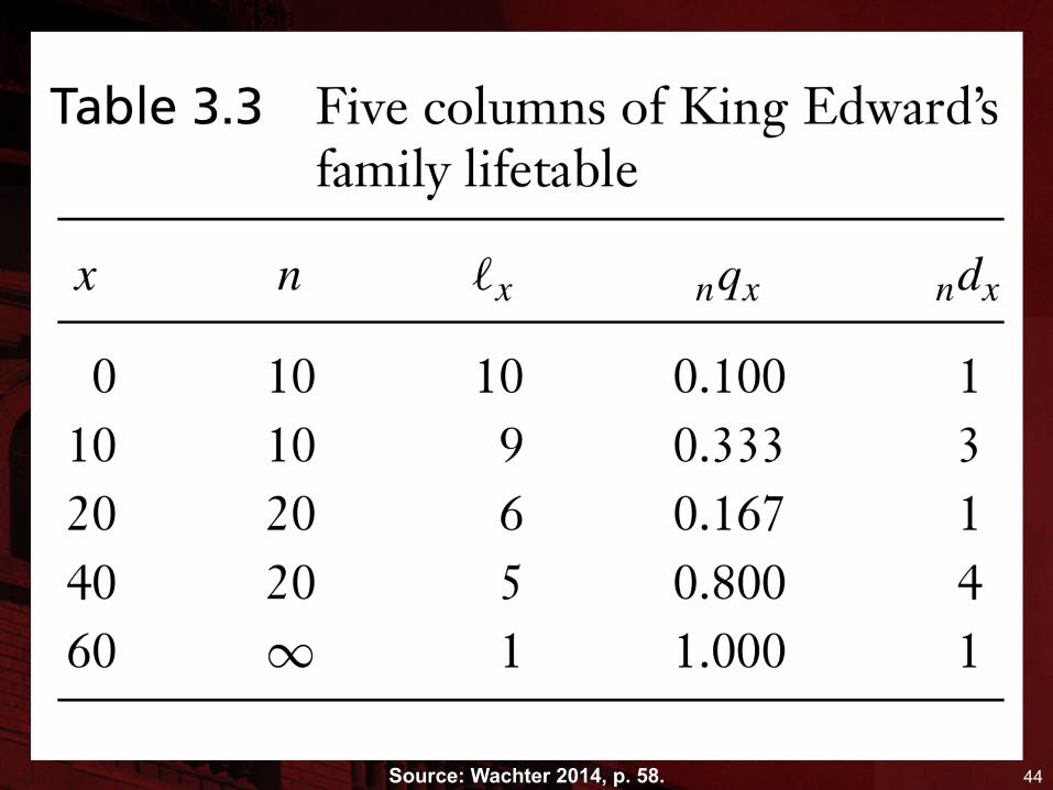
Probability of dying (nqx)• The column which follows lx in the lifetable

contains the probability of dying in the interval given that one is alive at the start

• This is the nqx measure

nqx = 1 − (lx+n / lx)

• For our example

– In the first age group, nqx = 1 − 9/10 = 0.100

– In the second age group, nqx = 1 − 6/9 = 0.333

42

Number of deaths (ndx)• We go on to insert a column which gives deaths

between ages x and x + n

ndx = lx − lx+n

• This column counts the lifelines that end in each age interval on the Lexis diagram

43


From nLx to ex• The remaining columns of the lifetable relate to

cohort person-years lived (CPYL)

• In order to calculate person-years, we need nax• nax tells us how many years within an interval

people live on average if they die in the interval

• This quantity is about half the width of the interval (n/2)

46

Cohort person-years lived (nLx)• With nax, we can calculate cohort person-years

lived between ages x and x+n (nLx )– Also called “big L”

– Think of “L” standing for life

• Big L is one of the four most important columns with– lx , “little l”

– nqx– ex

47

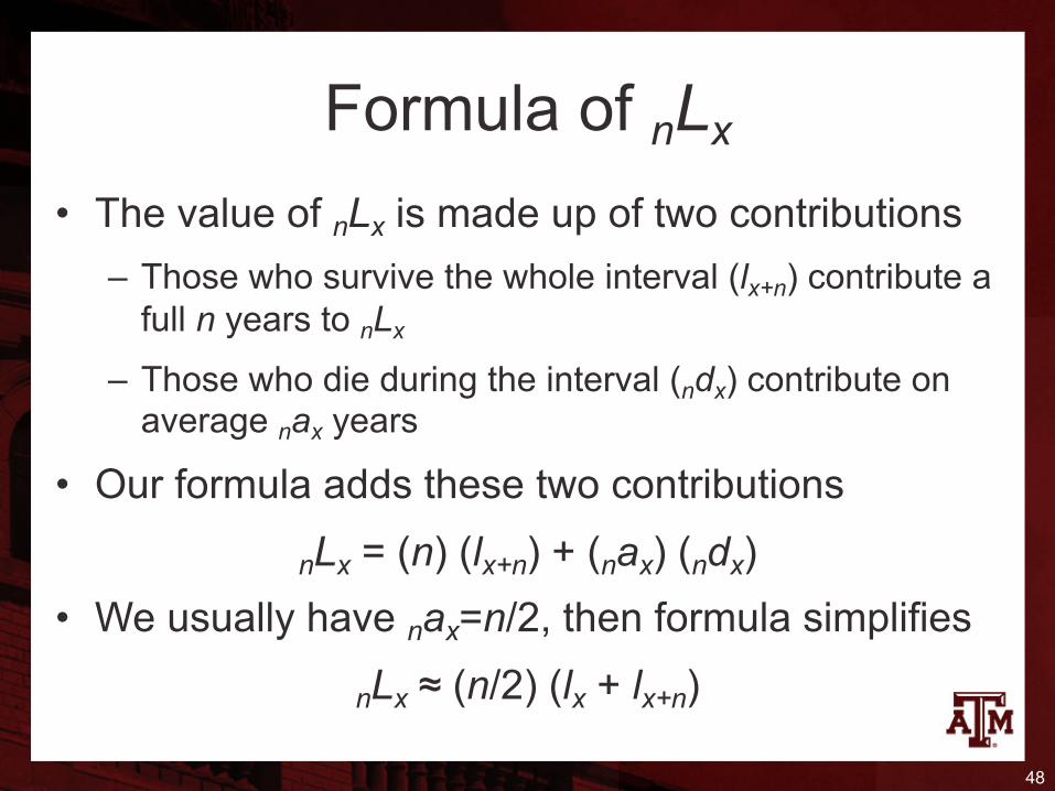
Formula of nLx• The value of nLx is made up of two contributions

– Those who survive the whole interval (lx+n) contribute a full n years to nLx

– Those who die during the interval (ndx) contribute on average nax years

• Our formula adds these two contributions

nLx = (n) (lx+n) + (nax) (ndx)• We usually have nax=n/2, then formula simplifies

nLx ≈ (n/2) (lx + lx+n)

48

nLx as the area under the lx curve


• With a smooth curve of lx, we can calculate nLx as the area under the lx curve between x and x+n

nLx

Death rate (nmx)• For the lifetable death rate (nmx), we divide cohort

deaths (ndx) by cohort person-years lived (nLx)

• The column nmx is the age-specific counterpart of the crude death rate (CDR)

• nmx is a rate, measured per unit of time

• The lifetable death rate measured over a very short interval starting at x is very close to the hazard rate

50

Remaining person-years of life (Tx)• We can obtain person-years of life remaining for

cohort members who reach age x (Tx)

• We simply add up all person-years to be lived beyond age x

• Tx is easiest to compute by filling the whole nLxcolumn and cumulating sums from the bottom up

Tx = nLx + nLx+n + nLx+2n + ...

51

Remaining life expectancy (ex)• The main use of Tx is for computing the

expectation of further life beyond age x (ex)

• The Tx person-years will be lived by the lxmembers of the cohort who reach age x

– So ex is given by the formula

ex = Tx / lx

• The expectation of life at age zero (at birth) is often called the life expectancy (e0)

52

Average age at death (x + ex)• ex is the expectation of future life beyond age x

– It is not an average age at death

• We add x and ex to obtain the average age at death for cohort members who survive to age x– Not all lifetables include x + ex

– The x + ex column always go up

• ex does not always go down– It often goes up after the first few years of life, because

babies who survive infancy are no longer subject to the high risks of infancy

53

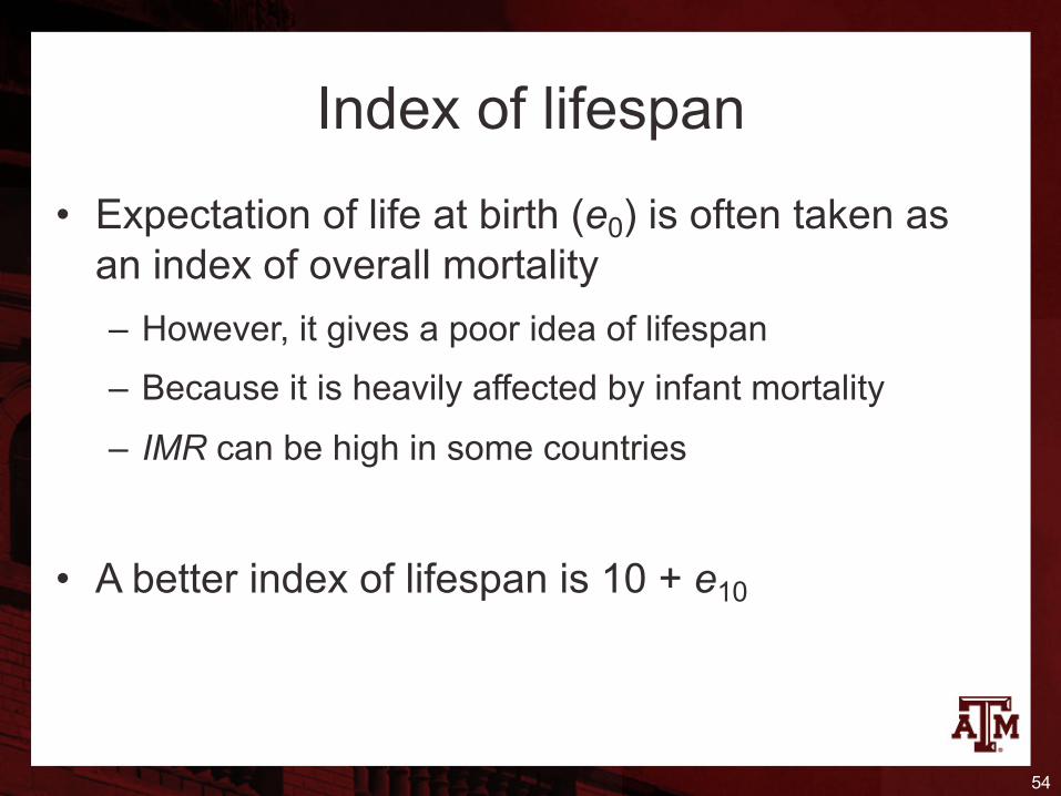
Index of lifespan• Expectation of life at birth (e0) is often taken as

an index of overall mortality– However, it gives a poor idea of lifespan– Because it is heavily affected by infant mortality– IMR can be high in some countries

• A better index of lifespan is 10 + e10

54


56Source: Wachter 2014, p. 58, 60.

Full cohort life table forKing Edward’s children

Shapes of lifetable functions

• Different lifetable functions express the same basic information from different points of view

• Demographers often have to– Start with entries for some column and work out entries

for another

– Start with bits and pieces of data from a few columns and solve for some missing piece of information

• Each lifetable function has a characteristic shape...

57

Typical shapes of lifetable functions


Cohort lifetable formulas


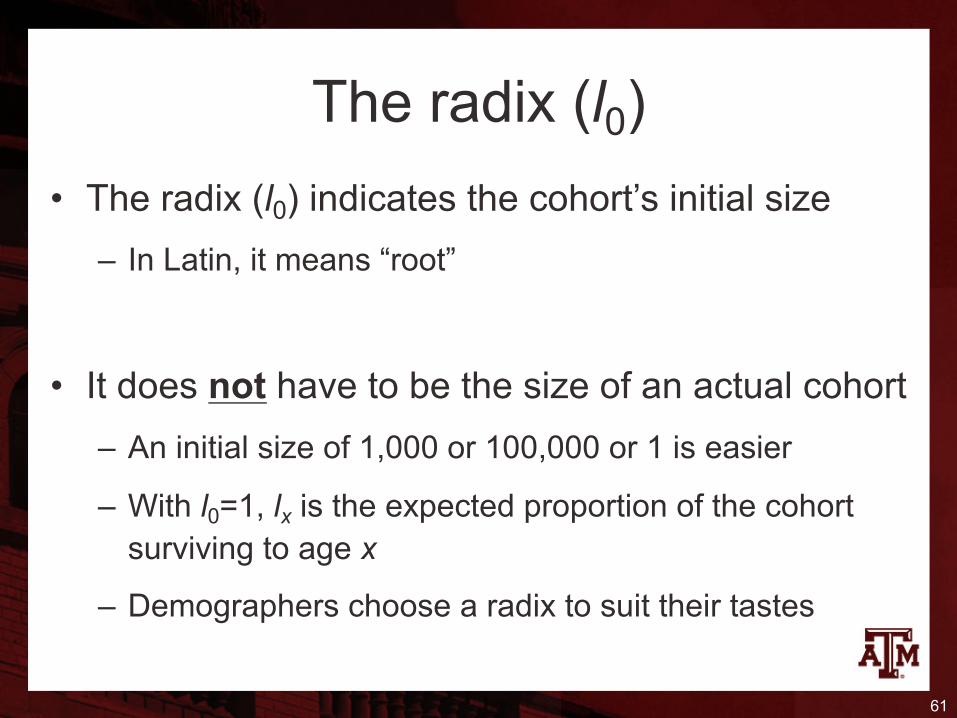
The radix (l0)• The radix (l0) indicates the cohort’s initial size

– In Latin, it means “root”

• It does not have to be the size of an actual cohort– An initial size of 1,000 or 100,000 or 1 is easier

– With l0=1, lx is the expected proportion of the cohort surviving to age x

– Demographers choose a radix to suit their tastes

61

Interpreting lifetable• The lifetable is used to follow a cohort through life

– l0 is seen as a random sample of the actual cohort

– Survival of the sample mirrors survival for the whole cohort

• Conceptually, it is good to picture an actual group of people (whole cohort or sample)– Starting with l0 members and living out their lives– Surviving

– Aging

– Dying62

Changing the radix• Some quantities alter and others remain the

same when changing the radix• Quantities that change (absolute numbers)

– lx– nLx– ndx

• Quantities that do not change (indicators)– nqx– nmx

– ex63

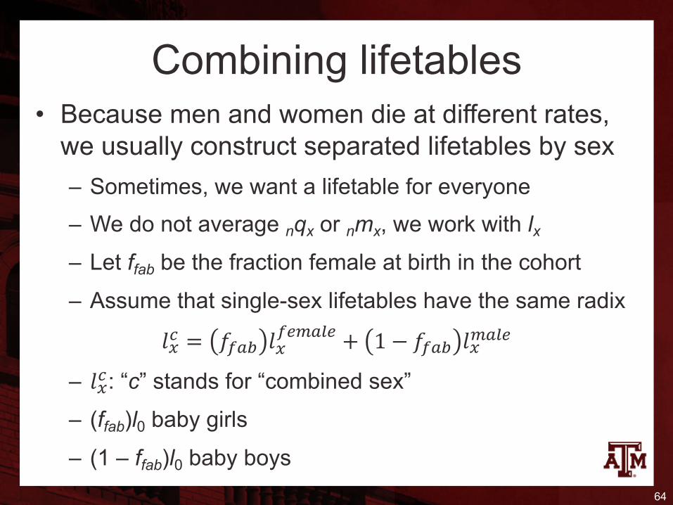
Combining lifetables• Because men and women die at different rates,

we usually construct separated lifetables by sex– Sometimes, we want a lifetable for everyone– We do not average nqx or nmx, we work with lx– Let ffab be the fraction female at birth in the cohort

– Assume that single-sex lifetables have the same radix

– !"#: “c” stands for “combined sex”

– (ffab)l0 baby girls

– (1 – ffab)l0 baby boys64

!"# = %&'( !"&)*'+) + 1 − %&'( !"*'+)

Annuities and insurance• Annuities and insurance are social institutions

that become familiar usually after school or college when starting a job or a family

• Earliest applications of lifetable methods in the 1600s and 1700s were to annuities

• Idea of a steady income (e.g., after retirement)

– You buy a policy from an annuity company for a single payment (P)

– The company agrees to pay you an annual benefit (B) for as long as you live

66

Annuities• The purpose of buying an annuity is to share risk

– You pay now and collect benefits as long as you live– If you die soon, the company wins– If you live long, the company loses

• The company sets the purchase price to break even or come out ahead– Examples here deal with “actuarially fair rates”, where

profit is zero– In practice, a margin for profit is added– The purchase price ought to depend on the age of the

buyer67

Annuities and lifetable• To derive formulas connecting P and B, we

imagine all lx members of a cohort buying annuities at some age x– Some members live long– Other members don’t live as long

• Over the first n years after purchase– Cohort members live a total of nLx person-years– Each one receiving a benefit B each year, for B(nLx) in

benefits overall

68

Formula for annuities• Over all future ages, total benefits amount to

B nLx + B nLx+n + B nLx+2n + B nLx+3n ... = B Tx

• The total purchase amount equals price per person (P) times the number of buyers (lx)

P(lx)

• Equating purchase to benefits impliesP lx = B Tx

P = B Tx / lxP = B ex

69

Need to consider interests• If an annuity with a benefit $10,000 a year

purchased at age 20 could cost a lot– If e20 = 50 years

P = B ex

P = 10,000 * 50P = 500,000

• Companies don’t charge so much, because– They invest money and earn interest while it is waiting

to pay future benefits– Time elapses between purchase and receipt of

benefits70

Considering interests• To consider interest, imagine the company

opening a separate bank account for each future n-year period– It invests money for early benefits in short-term

investments– It invests money for distant future in long-term

investments

• We calculate annuity price by estimating how much money the company must put into each account at the start– In order to have enough money to pay benefits from

that account when the time comes71

Interests for different accounts• For the first account, the company has to deposit enough

money to pay out benefits B(nLx) on average half-way through the first period– This leaves on average about n/2 years for money to grow

through compound interest– At compound interest, 1 dollar grows to (1 + i)n/2 dollars in n/2

years with interest rate i– So the company needs to deposit B nLx / (1 + i)n/2

• For the next account, money can earn interest for an average on n+n/2 years, so the deposit equals

B nLx+n / (1 + i)n+n/2

• When the cohort reaches age y, the deposit isB nLy / (1 + i)y–x+n/2

72

General formula with interests• The company needs to deposit for all accounts

• Lifetables with an open-ended interval starting at a top age xmax introduce a specificity– The rule is to replace n/2 with exmax

– People alive at the start of the interval will live about exmax further years

73

! "#$1 + ' "/) +

! "#$*"1 + ' "*"/) +

! "#$*)"1 + ' )"*"/) + ⋯

1 + ' "*,-./-

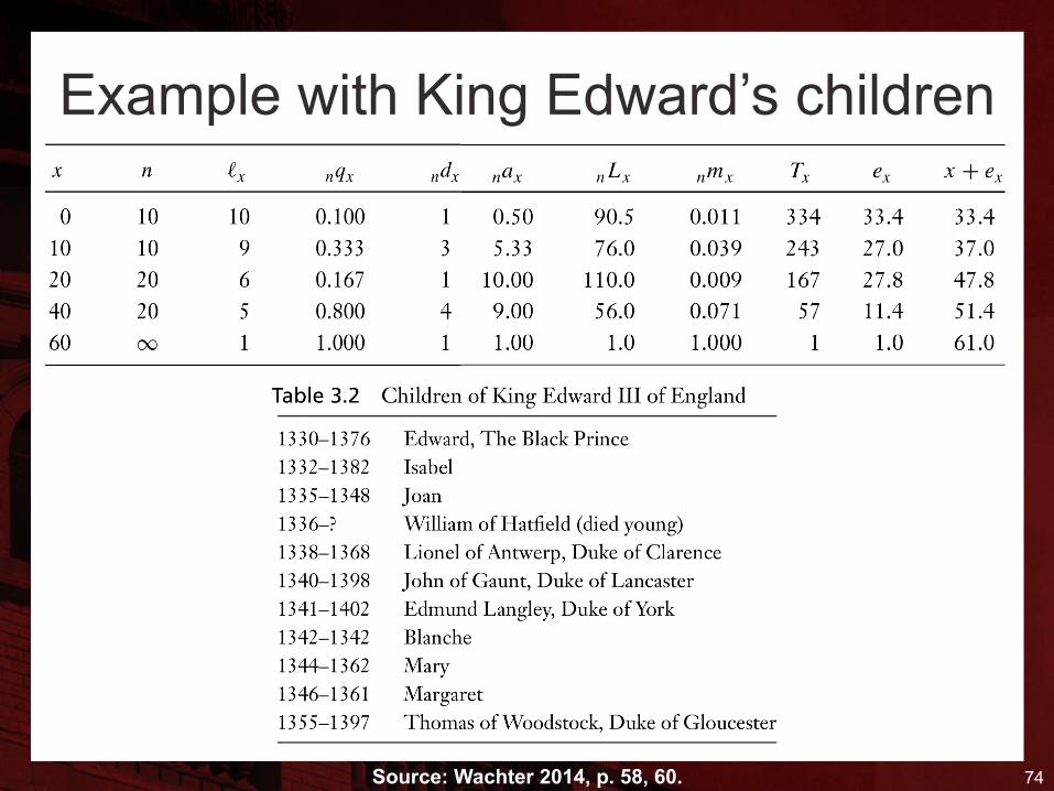
74Source: Wachter 2014, p. 58, 60.

Example with King Edward’s children

Example• Suppose King Edward III had bought annuities

with a benefit of £100 a year for all five of his surviving children when they were age 40– Interest per year = 10% = 0.1

– 20L40 = 56; n = 20

– ∞L60 = 1; exmax = 1

75

! "#$1 + ' "/) +

! "#$*"1 + ' "*+,-.,

= ! )0#101 + 0.1 )0/) +

! 4#501 + 0.1 )0*6 =

100 ∗ 561.1 60 + 100 ∗ 1

1.1 )6 = 2,159 + 13 = 2,172

Insurance policies• Insurance policies resemble annuities

– But the company promises to pay an amount once when you die, not year by year when you are living

– The purchase price (P) is paid at the start– All formulas are the same as for annuities– Except that death to cohort members (ndx) take the

place of person-years lived (nLx)

• Today companies usually sell term insurance, where the benefit is paid only to cohort members who die in the next year (1dx)

76

Variations• Annuities may be purchased at age x and start

paying benefits only at some later age z– This implies that the sum over terms nLy only starts at y=z

• Buyers may have a mix of ages– Each age can be treated separately and results added

together

• All these calculations require skills with lifetables

77

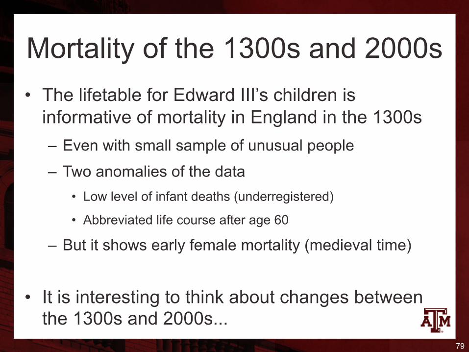
Mortality of the 1300s and 2000s• The lifetable for Edward III’s children is

informative of mortality in England in the 1300s– Even with small sample of unusual people– Two anomalies of the data

• Low level of infant deaths (underregistered)

• Abbreviated life course after age 60

– But it shows early female mortality (medieval time)

• It is interesting to think about changes between the 1300s and 2000s...

79

Changes in infant and old mortality• Infant and child mortality has dropped dramatically

over the last hundred years– Death of a baby has become an unusual event

• Life expectancies (affected by infant mortality) are no guide to maximum attained ages– Edward III’s children lifetable: e0 = 33.4

– Edmund Langley lived past 60 (but this was rare)

• Today large numbers of people live active lives into their late 80s and 90s– It changes attitudes about what it means to be old

80

References

Wachter KW. 2014. Essential Demographic Methods.

Cambridge: Harvard University Press. Chapter 3 (pp. 48–

78).

81

Documents

Ernesto F. L. Amaral