IEF

EIEF Working Paper 17/14

November 2017

Retirement in the Shadow (Banking)

by

Guillermo Ordoñez

(University of Pennsylvania and NBER)

Facundo Piguillem

(EIEF and CEPR)

EIE

F

WO

RK

ING

P

AP

ER

s

ER

IEs

E i n a u d i I n s t i t u t e f o r E c o n o m i c s a n d F i n a n c e

Retirement in the Shadow (Banking)∗

Guillermo Ordonez† Facundo Piguillem‡

December 2017

Abstract

The U.S. economy has recently experienced a large increase in life expectancy andin shadow banking activities. We argue these two phenomena are intimately related.Agents resort on financial intermediaries to buy insurance against an uncertain lifespan after retirement. When they expect to live longer they are more prone to rely onfinancial intermediaries that are riskier but offer better terms for insurance – shadowbanks. We calibrate the model to replicate the level of financial intermediation in 1980,introduce the observed change in life expectancy and show that the demographic tran-sition is critical to account for the boom both of shadow banking and credit that pre-ceded the recent U.S. financial crisis. We construct a counterfactual without shadowbanks and show that they may have contributed 0.5GDP, which is larger than the costof the crisis of around 0.2GDP.

JEL classification: E21. E44.

∗We thank seminar participants at the ITAM-PIER Conference on Macroeconomics in Philadelphia, theSED Meetings in Warsaw, RIDGE 2017 in Montevideo, Universitat Autonoma de Barcelona, Bank of France,University of Padova and University of St Andrews for comments. The usual waiver of liability applies.†University of Pennsylvania and NBER (e-mail: ordonez@econ.upenn.edu).‡EIEF and CEPR (e-mail: facundo.piguillem@gmail.com).

1 Introduction

Since 1980 and until the great recession in 2007 the US economy experienced a steepincrease in intermediated borrowing and lending, with household’s debt growing from1GDP to 1.7GDP. This “credit boom” has drawn the attention of both policymakers andscholars, particularly in relation to the magnitude of the subsequent financial crisis. Mul-tiple reasons have been proposed, ranging from an atypical influx of foreign funds, i.e,the international savings glut, to pure financial speculation. Absent any fundamentalimprovement in the economy these explanations tend to consider the credit boom as ex-cessive and then just detrimental for the economy in inducing a potential painful crisis.

In this paper we analyze the contribution of a domestic factor that has gone unnoticedso far but may explain this credit boom: the increase in life expectancy. In the UnitedStates, life expectancy increased dramatically from 74 years to around 79 years in a shortperiod of three decades. We argue that this increase in the demand for precautionarysavings has led to the arrival of new and more effective ways to supply insurance, such asshadow banking. We show that both of these developments are needed to account bothfor the observed expansion in private borrowing and the evolution of interest rates.

Our findings suggest that the observed patterns of credit may have been an efficientreaction of financial markets to demographic changes instead of the result of bankingwrongdoing. Furthermore, we provide a measure of the benefits of shadow banking onfacilitating those patterns, contributing to the discussion about the desirability of the newfinancial landscape in economies that experience structural and demographic changes.

Savings for retirement is indeed one of the most important reasons for the need offinancial intermediation. A large fraction of total wealth is held by retirees. Wolff (2004)documents that more than a third of total wealth in the United States is held by householdswhose heads are over age 65. Consistent with this finding, Gustman and Steinmeier (1999)show that, for households near retirement, wealth is around one third of lifetime income.Even before retirement there is strong evidence that most people’s savings are intendedto be use after retirement.1

As workers save for retirement, they provide funds that can be used to finance pro-ductive investment opportunities and to cover the liquidity needs of those who in thepast saved for retirement. The cost of the first activity, which we denote as operation cost,is the cost of finding the best available investment opportunities to allocate the funds, and

1Two classical papers making this point are Gale and Scholz (1994) and Kotlikoff and Summers (1981).

1

includes the process of finding productive opportunities, monitoring the management ofprojects and administering payments. The cost of the second activity, which we denote asliquidity cost, is the cost of transforming long-term risky loans into short-term safe assetsthat can be liquidated at stable nominal conditions in relatively short periods of time incase a fraction of investors larger than the one that are expected to withdraw funds (thosethat are in their retirement age) choose to withdraw their funds in advance.

Since the eighties, U.S. households’ assets held in retirement funds duplicated as afraction of GDP (from 55% in 1980 to 110% in 2010). Even though the increase in lifeexpectancy induced a large increase in the demand for safe assets that can be providedby financial intermediaries, we document that at the same time there was also a largeincrease in the supply of safe assets. We show that the cost of intermediation, measuredby the spread between lending rates and deposit rates, declined from a stable level of 4%in 1980 to around 3% before the recent financial crisis. Relying on Philippon (2015), whoshow that operation costs have been constant in the financial sector for almost a century,we conclude that the bulk of the decline in the cost of intermediation in the last threedecades can be accounted for by a reduction in liquidity costs.

We argue that this decline in liquidity costs has been driven by the use of financialinstruments channeled at the heart of what became known as “shadow banking.” Secu-ritization, for example, is the backbone of shadow banks. It allows for the creation ofassets that, even though backed by productive risky loans, are designed to be informa-tion insensitive and to be liquidated with the same facility than government bonds andother liquid assets, which are backed instead by unproductive safe taxation. Furthermore,shadow banking allows banks to escape blunt, and potentially restrictive, regulatory con-straints that inefficiently impose a fraction of their assets to be invested in unproductiveasset classes, such as government bonds.

Are these two changes quantitatively large enough to accommodate the large increasein financial intermediation experienced by the United States since 1980? What are theindividual contributions of higher retirement needs and shadow banking on growth andoutput? We show in a calibrated model with financial intermediation that the higher de-mand for safe assets (from an increase in insurance motives due to higher life expectancy)generates not only an increase in accumulation of assets, but also a decrease in the returnto the safe assets. In turn, the decrease in the returns, together with the longer expectedlife, increases the benefits to search for higher yields. Since the shadow banking technol-ogy pays higher returns (due to lower liquidity costs), there is a switch of savers from

2

traditional to shadow banking that allows for a larger supply of safe assets. We show thatthis mechanism can indeed quantitatively accommodate the large increase in financialassets as a fraction of GDP experienced by the United States.

As we need a model that consistently displays borrowers and lenders and their in-tereactions, we construct an overlapping generations model with heterogeneity on thebequest motives of individuals: individuals with high bequest motives hold capital andborrow from individuals with low bequests motives. All borrowing and lending is chan-neled through financial intermediaries that have to guarantee savers (lenders) that theirassets are safe, which has an opportunity cost of not investing in more productive, butriskier, options – a liquidity cost. Securitization provided the technology to transform apart of those more productive and riskier assets into safe assets, then reducing the liquid-ity cost. The savers (lenders) can choose between two types of financial intermediaries:traditional banks (TB) and shadow banks (SB). The difference between them is that SBexhibits a lower liquidity cost (due to more securitization) that translates into higher in-terest rates paid over deposits. However, finding and operating with SB is more costlythat finding and operating with TB. Thus, savers would choose to save for retirementthrough SB only if the present value of the difference in returns is larger than the searchcost. As a result, for given returns differential, as the life expectancy increases, so it doesthe present value of the gains to move to shadow banks. In short, a higher life expectancytriggers an appetite for yields, and shadow banks can fulfill such appetite.

We calibrate the economy to 1980 and input the change in life expectancy to generate acounterfactual for 2005. We show that isolated (direct) impact of the increased demand forsafe assets does generate more financial intermediation, but imposes an important down-ward pleasure on safe asset’s returns that partially compensates the expansion of the fi-nancial sector. However, the downward pressure of returns triggers a switch of saversfrom traditional to shadow banks (appetite for yields) that allows for an increase in thesupply of safe assets, increasing further the intermediated quantities by the financial sec-tor while preventing the fall on interest rates.

Only including both changes we can account for the observed evolution of house-holds’ debt over GDP and total financial assets held in the economy, with an increase ofaround 75% in both figures. Absent the switch to shadow banking, the change in lifeexpectancy would only account for an increase of around 10% in households debt overGDP and 6% on total financial assets. We also decompose the impact of shadow bankingon output. Absent shadow banking, steady state output would have grown only half of

3

what it grows when both forces are combined. These results highlight the importance offirst understanding the determinants of financial markets to then assess their impact onaggregate dynamics.

Finally, as we are able to construct a counterfactual economy without shadow banks,we can compute the output gains from the lower interest rate spreads induced by thisfinancial innovation and weight them against the output costs of a crisis that is assumedtriggered by the operation of shadow bank activities. We find that, from 1980 to 2007, theexistence of shadow banking increased output by half of 2007 GDP. This number can beput in context when compared to the cost of the great recession. The literature computesthis cost by the difference between the potential GDP constructed by the CBO and therealized GDP. If we assign the cause and depth of the recession completely to the existenceof shadow banking, its cost is 0.23 of 2007 GDP. This cost is however overestimated as ittakes the potential GDP based on the existence of shadow banks to compute the costsof shadow banks, while a more consistent estimate comes from comparing a benchmarkwithout shadow banks and without crisis with the realized output after the crisis. Thisexercise delivers a cost of 0.16 of 2007 GDP. As a summary, even if the crisis were only dueto shadow banks, still the economy had gained around 0.3 of 2007 GDP by its existence.

Related Literature: We contribute to the recent academic and policy discussion onthe effects of shadow banking for macroeconomic aggregates. While most of this debatefocuses on the costs of shadow banks in terms of inducing crises and making financial sys-tems fragile, much less is known about their potential positive macroeconomic effects. Asin our paper, Moreira and Savov (2015) highlight that shadow banking improves liquidityprovision during booms and enhances growth, but at the cost of increasing fragility. Intheir case, shadow banking expands during periods of low uncertainty in the economyand collapses when uncertainty increases. In contrast, we study the role of higher re-tirement saving needs and a higher demand for safe assets in boosting the use of shadowbanks, which provide a better, but more fragile, alternative than traditional banks for theirprovision. Even though we focus on the positive macroeconomic effects of the run up ofshadow banking, not on its demise, we are able to provide an estimate of the net gainsof shadow banking in the U.S. since the eighties even when accounting (and completelyblaming shadow banks) for the financial crisis in 2008.

Similarly, we do not discuss optimal regulation of shadow banking, but provide aquantitative assessment of its benefits and its costs in case the crisis would have beencompletely triggered by its existence. For an interesting macroeconomic model of optimal

4

regulation of shadow banking see Begenau and Landvoigt (2017).In contrast to a rich literature (such as Caballero (2010), Caballero, Farhi, and Gour-

inchas (2016) and Carvalho, Ferrero, and Nechio (2016)) that argues that the increase inthe demand for safe assets may have come from foreign countries saving needs (the well-knowing “savings glut” hypothesis) in this paper we focus on the increase on the demandof safe assets coming from higher needs for retirement of U.S. residents. Interestingly, alarge part of the saving glut from foreign countries has been accommodated by an increasein U.S. government debt and the provision of U.S. government bonds. Shadow banking,then, has had a primary role in accommodating the domestic demand for safe assets, andindeed we find not only that these forces are substantial quantitatively but also that acalibrated model can account for most of these changes.

In this sense, the paper contributes to the discussion of the volume of retirement sav-ings once we add financial intermediaries and their cost of intermediation explicitly. Eventhough there is a rich literature studying the relevance that savings for retirement pur-poses have on investment, output, and interest rates in macroeconomics, the impact offinancial intermediation on those relations is less explored, with the exception of Mehra,Piguillem, and Prescott (2011). We extend their environment by making the financial sec-tor, in particular the roles of traditional and shadow banking, endogenous.

Our work is also complementary to papers that micro found the effects of shadowbanking on reducing liquidity costs. Gorton and Ordonez (2014) show that securitiza-tion, the tool most used for shadow banking activities, through pooling and tranching,reduced the incentives of information acquisition and allows risky assets to be combinedand traded as safe assets, providing “safety” at lower costs. Similarly, Ordonez (2014)shows that shadow banking arises as an equilibrium response to regulations that are ex-cessively, and inefficiently, constraining in times in which reputation concerns operate infinancial markets, which happens for example when expected future business opportuni-ties are very promising. We use these insights to understand how the increase in shadowbanking was at the forefront of the observed decline in the liquidity cost.

In our model shadow banking provides safety at a lower cost by using a complex andcostlier technology to transform risky assets into safe assets. The extra cost of this tech-nology comes from the complexity needed to pool and tranche risky assets, its fragilityand its predisposition to be subject to moral hazard. When the needs for safe assets in-crease, the relative benefits to operate with shadow banking increases and then there isa transition away from traditional banking activities. In this story we have abstracted

5

from regulatory arbitrage, but we could modify the main trade-off to incorporate theseconsiderations. Ordonez (2017), for example, highlight that shadow banking is beneficialbecause it allows an escape from blunt regulations at the cost of excessive risk-taking.Farhi and Tirole (2017) discuss how traditional banking is sustained on complementari-ties between costly public supervision and beneficial public liquidity guarantees, and howregulation (taxes and subsidies, ring fencing, etc) can accommodate these forces to avoida migration towards shadow banking activities.2

Next we introduce a macroeconomic model with savings for retirement and financialintermediation, calibrate it and decompose the effects of shadow banking on welfare, out-put and the accumulation of assets.

2 Model

2.1 Environment

We study an overlapping generations economy populated by households that work ona competitive productive sector, save for retirement through financial intermediaries andare taxed by the government.

2.1.1 Households

Each period a measure (1 + η)t of agents are born, where η is the population growth rate.Agents born at age j = 0 and live with certainty for T periods, during which they canwork an inelastic amount of hours without utility cost. After age T they cannot longersupply labor (they retire) and die with constant probability 0 < δ < 1 thereafter. When anagent dies at age j it may leave bequest bj that generates α ≥ 0 units of consumption utilityper unit of bequest. Agents discount the future at the rate 1

β− 1 and are heterogeneous

on the intensity of their bequest motive, α ∼ m(α). Assuming that households valuelogarithmically the consumption at age j, which we denote by cj , their present value ofutility at a calendar period t is,

T∑j=0

βj log ct+j,j +∞∑

j=T+1

βj(1− δ)j−T−1[(1− δ) log ct+j,j + δα log bt+j,j] (1)

2Other papers that focus on the interactions between regulation and shadow banking include Harris,Opp, and Opp (2014), Plantin (2015) and Begenau and Landvoigt (2017).

6

As labor does not generate any disutility, each generation j = 0, 1, ..., T (of measure 1)supplies one unit of labor inelastically. Hence L = T .

As is clear from equation (1), we assume the “joy-of-giving” type of bequest motive.This motive, however captures several forces. First, it is consistent with the empirical ob-servation that people leave equal bequest to their heirs. Second, as shown by De Nardi,French, and Jones (2010) and De Nardi, French, and Jones (2015), agents save after re-tirement as a precaution against medical expenses. As health is a normal good, the joy-of-giving specification also delivers this concern in a simple way. Thus, the reader mustinterpret the parameter α as capturing both precautionary savings against large potentialhealth shocks at old age and pure bequest motives. As pointed out by De Nardi, French,and Jones (2015) it is almost impossible to properly disentangle the contribution of eacheffect.3 Besides being instrumental in simplifying the solution of the model, our chosenspecification is also useful to capture non-trivial effects of changes in the age structureover savings.4

We have also assumed an exogenous retirement age as a simplifying assumption thatresembles the observed pattern of retirement in the U.S. As Bloom, Canning, and Moore(2014) argue, as life expectancy increases there are two effects affecting the retirementdecision: 1) workers can extend their working life to compensate the longer life afterretirement but, 2) due to the increase in labor productivity, the income effect increasesthe demand for leisure, and thus, decreases the retirement age. Hence, the final effect ofincreasing life expectancy in retirement age is ambiguous. In fact, Costa (1998) shows thatthe retirement age in the US, and many countries, has been continuously decreasing inthe last 100 years, which points to the dominance of the income-wealth effect. As a result,with this assumption we would be understating the effect of aging on savings.5

Finally, one may wonder why we focus on the period after 1980 given that life ex-pectancy has increased steadily during the twentieth century. However, as shown by theU.S. Social Security Administration, the life expectancy conditional on reaching 65 yearsold has been constant to 13 additional years until 1980 and then it has increased steadyfrom 13 to 17 additional years until 2010.

3See also Lockwood (2015) for an attempt to identify each component.4For instance, if we had assume that agents are perfectly altruistic with respect to their offspring (“Barro-

Becker” type of bequest motive), individual savings would be independent of both life span and survivalprobabilities. This would be at odds with the empirical evidence, as discussed by De Nardi, French, andJones (2009).

5See also Bloom et al. (2007).

7

In the balance growth path we only need to analyze the problem of an individual bornat t = 0, as the problem of any other individual born at t is simply ct,j = (1 + γ)tc0,j . Wewill denote c0,j simply as cj when studying the balance growth path.

In terms of income, individuals have three sources. First, they receive labor income yjfor the labor provided at age j during the first T years of their life (working age). Second,we assume that the bequest bj that agents leave upon death at age j is equally distributedamong all agents alive of age TI < T . Thus, every agent receives an inheritance, b, at ageTI . Finally, individuals may receive a transfer Tri from social security every period afterretirement. Denoting agent i’s saving returns by ri and assuming a labor income tax τ , theagent i′ that born at t = 0 has a consolidated total wealth at birth on the balance growthpath of,

vi0 =T−1∑j=0

(1− τ)yj(1 + ri)j

+b

(1 + ri)TI+

(1 + ri)

ri + δ

Tri(1 + ri)T

(2)

Notice that the only source of individual risk is the agent’s life span. Thus, the onlyreason for saving is to hedge the risk of outliving one savings: there are only savingsfor retirement. We are abstracting from aggregate risk, which is not insurable in a closedeconomy, and other sources of idiosyncratic risk, like unemployment or health shocksduring the working lifetime. From this point of view we are underestimating the amountof precautionary savings. Since all savings, independently of their original purpose, canbe used in principle to hedge any kind of risk, before and after retirement, the bias wouldbe small as long as the survival risk is sufficiently strong. As Gale and Scholz (1994) andKotlikoff and Summers (1981) show, between 75% and 90% of individual savings can beexplained by retirement reasons only.

In order to capture in the simplest possible way the different life strategies that dif-ferent individual use to hedge the retirement risk, we restrict the households’ choice setto two alternatives, 1) to buy annuities from financial intermediaries or 2) to self-insure.More importantly, we assume that households can only choose among these alternativesat age j = 0, and not at any other age j > 0. This assumption is made for simplicity,otherwise, as it will be clear later, it would be optimal for every household to follow thestrategy with high returns when young and switch to the strategy with better insurancejust before retirement. However, since Mankiw and Zeldes (1991) there is ample evidencethat most households do not ever hold stocks and prefer to keep all their financial assets

8

in riskless alternatives (this is known as participation puzzle). Even those householdsthat decide to include stocks in their portfolios do not drastically change their strategiesas they age.6

To be concrete, every agent have access to the following two strategies:

1) Strategy B: Bank-insurance: Sign an annuity contract with a financial intermediary(a Bank). An annuity contract between an agent and a financial intermediary specifies thepayment that the agent must make to the intermediary during the agent’s working age andthe payment that the intermediary must make to the agent when the agent retires. This is, theagent consumes cj as long as the agent is alive and leaves bj to the heirs contingent ondying. There are two possible banks that the agent can choose to sign this annuity, a tra-ditional bank (TB) or a shadow bank (SB). We assume that choosing and understandinga shadow bank is more costly for agents such that they have to pay a utility cost κ to signthe contract. We will describe how these two types of banks differ in their liquidity costsin more detail later.

2) Strategy S: Self-insurance: The agent saves, in equity or in bonds, part of her in-come while working and lives out her savings after retirement bequeathing any un-spentsavings.

In short, households choose their retirement strategy when they are born and, basedon this decision, they choose the sequence of consumption during their working life andafter retirement.

2.1.2 Productive Sector

The productive sector operates every calendar period t with a Cobb-Douglas productionfunction with exogenous growth rate γ,

Yt = Kθt (ΓtLt)

1−θ

Γt+1 = (1 + γ)Γt

where K is the aggregate stock of capital in the economy, L is the aggregate supply oflabor and Γ is the average labor productivity. Thus, θ is the share of capital income over

6Fagereng, Gottlieb, and Guiso (2017) argue that a combination of participation costs and a small “disas-ter” probability are needed to rationalize the low change in investments. Alvarez, Guiso, and Lippi (2012)show that not only participation costs are needed, but also observational costs.

9

total income. Labor and capital markets are competitive, which implies that the rental rateof the inputs equals their respective marginal productivity.

δk + re = FK(Kt,ΓtLt)

yt = FL(Kt,ΓtLt)

where δk is the capital depreciation rate. Along the balance growth path, Kt+1 = (1 + γ)Kt

and from the law of motion of capital investment is Xt = (δk + γ)Kt.

2.1.3 Financial Intermediation

On the financial sector, we assume that perfectly competitive banks offer annuity contractsto households (those following strategy B) to save for retirement. They specify the grossrate 1 + r that a household receives per unit of saving made during the working age.With these savings, the bank can invest either in “safe government bonds” that pay withcertainty a unit gross rate 1 + rL per unit of bond or in a continuum of “risky loans’ thatpay a unit gross rate 1 + re > 1 + rL per unit of loan, but only with probability 1 − sb, aswith probability sb the loan defaults and pays nothing. The expected return of bonds isthen rL, while the risk-adjusted expected return on loans is re ≡ (1− sb)(1 + re)− 1. Eachbank takes these returns as given.

We denote the total savings obtained by a financial intermediary from agents choosingannuities by D, and all assets by A. We also denote the fraction of assets that the bankchooses to invest in loans by f . Finally, we assume that banks face a constant returns toscale technology, with a constant marginal cost of operation φ per unit of asset managed.

We impose liquidity considerations that put an upper bound on how much a bankcan invest in loans while still obtaining savings. To capture these considerations in asimple way, we assume that banks are subject to potential coordination problems, underwhich all savers (agents that withdraw because they are retired and also agents duringtheir working life) can decide at a moment to withdraw their funds (a bank run). In suchevent, if a bank does not have enough funds to cover these withdrawals, it must defaultcompletely on all depositors. This is naturally a very extreme assumption that capturesvery extreme forms of fire sales or trade freezes but simplifies the exposition greatly.

We assume that a bank is completely insulated from this possible coordination failureif it can liquidate enough assets at face value. In such event the bank can resort to all bondsand to a fraction z of the loans. This fraction z captures the easiness to liquidate (sell or

10

collateralize) existing loans, considering that asymmetric information makes trading ofloans difficult and costly. In contrast, all government bonds can be easily liquidated andused to cover withdrawals. Then, for a given rate r, the bank is resilient (and thus notsubject to a bank runs) as long as,

[zf(1 + re) + (1− f)(1 + rL)]A ≥ (1 + r)D (3)

The zero-profit condition of the perfectly competitive financial intermediaries can beexpressed as

[f(1 + re) + (1− f)(1 + rL)− φ]A = (1 + r)D (4)

Finally we assume no arbitrage (agents can buy bonds at no cost), which implies that

r = rL,

, and that securitization becomes more difficult as bonds are a lower fraction of the bank’sportfolio, this is z(f) such that ∂z

∂f< 0. As an example, assume

z(f) = eψf

1−f

This function is a case in which z declines as f increases. Furthermore, the lower is ψ thebetter is the securitization technology.

Each financial intermediary chooses how much to invest A∗ (taking as given the fundsD obtained from agents choosing strategyB), the fraction f ∗ of those investments in loans(taking as given the return re) and the interest rate r∗ to pay to savers (taking as giventhe securitization technology ψ). The next proposition summarizes the optimal choices byfinancial intermediaries.

Proposition 1. If operational costs are not high, (re > φ) a bank invests all deposits,A∗ = D, while f ∗ and r∗ jointly solves

z(f ∗) =1 + r∗

1 + re(5)

11

and

φ ≡ re − r∗ =φ

f ∗(6)

where f ∗ and r∗ are increasing with securitization (decreasing in ψ).

Proof. When re > r the objective is to maximize f subject to the liquidity constraint(3), z(f)(1 + re) ≥ (1 + r). In our example this implies

f =log(

1+r1+re

)ψ + log

(1+r1+re

)and subject to the zero-profit condition (4).

As from equation (5) f decreases with r and from equation (6) f increases with r, thereis a unique equilibrium. As, fixing r, the fraction f increases as ψ decreases, then both r∗

and f ∗ increases as φ decreases (as securitization becomes easier). QED

Combining the equilibrium conditions (5) and (6), in our example we can rewrite therisk-adjusted interest spread as

φ = φ

[1 +

ψ

log(

1+re1+r

)] . (7)

The risk-adjusted interest spread has two main components: 1) the physical cost ofproduction, represented by the value added component, φ and 2) the liquidity component.This last component depends on the securitization technology, decreasing as ψ decreasesand securitization becomes easier.

Traditional and Shadow Banks: There are two technologies available in the economy,that differ in how loans are packaged, pooled and tranched to be traded as safe assetsand easily liquidated in case of runs (perfect substitutes of bonds). We assume that somebanks operate with ψTB while others with ψSB < ψTB. We refer to the former as traditionalbanks and the latter as shadow banks because a reason these banks may face differenttechnologies is that they may be constrained by different regulatory constraints, based onthe activities they perform. As it is clear from the previous analysis, and essential for ourquantitative exercise, shadow banks can invest a larger fraction of their portfolio in moreproductive loans, face less liquidity costs and offer a larger return to their investors.

12

2.1.4 Government

The government consumes a constant proportion g of output (which is not valued bythe consumers), follows a committed debt policy DG

t , which is independent of prices andquantities in the economy and pay an average social security transfer of Trt. The govern-ment collects taxes on labor income to balance the budget,

τytLt + (DGt+1 −DG

t ) = gYt + Trt + rLDGt (8)

We will assume hereafter that the social security transfer after retirement is a fractionssi of the last wage yT at retirement, which may be conditional on the saving decisions ofindividuals, i ∈ {B, S}. This is,

Tri,t = ssiyT,t.

Note that keeping revenue and spending constant, the above constraint implies thatchanges on the debt policy would have an impact on returns and aggregate quantities.Along the balance growth path DG

t+1 = (1 + γ)DGt .

2.1.5 Aggregates and Definition of (Stationary) Equilibrium

Next, we define aggregate variables and the stationary equilibrium. In what follows wefocus on steady state comparisons, but in Section 5.1 we study the transition of this modeland show that for our quantitative analysis the comparison of steady states capture mostof the main benefits of shadow banking after the increase in life expectancy experiencedin the US since the eighties.

First we specify aggregates along the balance growth path. Distinguish by i ∈ {B, S}agents according to their saving strategy. LetAi be the stationary set of agents α choosingstrategy i, µi(α) = m(α) if α ∈ Ai and define µi =

∫α∈Ai m(α)dα. As in every period t a

density (1 + η)tm(α) of agents are born and their survival probabilities are exogenous, thedensity of agents of age j is given by

µij(α) =

{µi(α)

(1+η)j−t if j ≤ T(1−δ)j−T−1µi(α)

(1+η)j−t if j > T.

We use these measures to obtain aggregates for each agent type i, as functions of (re, b).

13

C(re, b) =∑i=S,B

∞∑j=1

∫cij(r, b;α)µij(α)dα

WB(re, b) =∞∑j=1

∫wBj (r, b;α)µBj (α)dα

W S(re, b) =∞∑j=1

∫wSj (r, b;α)µSj (α)dα

B(re, b) =∑i=S,B

∞∑j=T+1

δ

∫bj(r, b;α)µij−1(α)dα

Lt =T−1∑j=0

(1 + η)t−j

where C is aggregate consumption along the balance growth path, wB and wS are theindividual net worths for agents following strategies B and S, respectively; WB and W S

t

are the corresponding aggregates, B is the aggregate bequest and Lt is total labor supply.

Definition 1 Stationary Equilibrium.Given fiscal policies {g, ssi, DG}, a stationary equilibrium is characterized by saving decisions

{{BTB, BSB}, S}, individual allocations {c(α), w(α), b(α)}∀α≥0, aggregate allocations {Y,B,C,X,K}and prices {y, re, rL, r} such that,

1. Given prices {y, re, rL, r} and fiscal policies {g, ssi, DG}, the individual allocations {c(α), w(α), b(α)}∀α≥0

solve the consumer-saver problem: households choose their retirement plan and consumptionpath to maximize utility.

2. Banks choose r and their portfolio allocation to maximize profits.

3. Factor prices are equal to marginal productivities.

4. The government chooses τ to balance the budget.

5. Markets clear,

• Feasibility: Y = gY + C(re, b) +X + φWB(re,b)1+r

• Assets market: WB(re,b)1+r

+ WS(re,b)1+re

= DG +K

14

• Bequest=inheritance: b = (1 + γ)TIB(re, b)

2.2 Equilibrium Characterization

We solve the equilibrium backwards. First we solve for the consumption path conditionalon each saving choice. Then we show the optimal saving decision.

We first consider strategy B. The following analysis is regardless of whether the in-dividual chooses to use traditional or shadow banking, as these cases will only changethe received interest rate, r. Any household following strategy B would maximize theutility (equation 1) subject to equation (2). In the appendix we show that the solution ischaracterized by:

cBj = CBβj(1 + r)jvB0 (9)

bBj = αCBβj(1 + r)jvB0

for some constant CB > 0. Notice that b can be considered as another consumption good,so that intratemporal optimality imposes b = αc. Furthermore, households signing annu-ities perfectly smooth consumption. For instance, if β(1 + r) = 1 a household followingstrategy B would experience constant consumption through its life and would leave ex-actly the same bequest, independently of how long the household has lived. The aboveconsumption plan implies the following pattern for the net worth of a household choosingstrategy B.

wB0 = 0 (10)

wBj = (wBj−1 − cBj−1 + (1− τ)yj)(1 + r), 1 ≤ j ≤ T, j 6= TI

wBj = (wBj−1 − cBj−1 + (1− τ)yj)(1 + r) + b, j = TI

wBj =∞∑t=0

(1− δ)t−1

(1 + r)t[(1− δ)cj+t + δαbj+t − ssByT ] , j > T

Agents are born with zero wealth, they work and lend to the financial intermediary anynon-consumed income, which generates a return r. At age TI each household receive aninheritance which is mostly saved, thus the net worth jumps at this age. After retirement

15

the financial intermediary pays the signed agreement, hence the net worth for the house-hold is the present value of the contract.

Now we consider strategy S. Households in this case must plan how much to savefor retirement and how to spend those savings after retirement. This can be consideredas two separated problems. We solve it backwards, i.e. we first solve the problem afterretirement.

Given any net worth level after retirement, since all bequest are accidental bj = wj forall j ≥ T . Hence, the problem after retirement when self-insuring solves

V (w) = max{log c+ (1− δ)βV (w′) + δβα logw′}

subject to

c+w′

(1 + re)≤ w

where re is the risk-adjusted return on equity.Given the assumed functional forms for consumption and bequest, it is straightfor-

ward to verify that the value function is logarithmic in w. That is,

V (w) = ν1(α) + ν2(α) logw

with ν2(α) =1 + αβδ

1− (1− δ)β

Simple calculations show that the optimal consumption plan and the implicit optimalbequest plan are

c = w/ν2(α)

w′ = (1 + re)(w − c+ ssSyT ). (11)

Given this solution after retirement, the optimal plan at entry in the labor force solves

maxT−1∑j=0

βjlogcj + βTV (wT )

16

subject toT−1∑j=0

cj(1 + re)j

+wT

(1 + re)T≤ vS0

with vS0 given by equation (2). The solution is

cSj = CSβj(1 + re)jvS0 , j < T (12)

wST = [1−T−1∑j=0

CSβj](1 + re)TvS0

During working age, the net worth by agents that follow strategy S evolves as

wS0 = 0 (13)

wSj = (wSj−1 − cSj−1 + (1− τ)yj)(1 + re), 1 ≤ j ≤ T, j 6= TI

wSj = (wSj−1 − cSj−1 + (1− τ)yj)(1 + re) + b, j = TI

There are two features of this economy that are apparent comparing equations (12) and(11) with (9). First, since re > r before retirement the consumption of self-insuring house-holds grows faster that the consumption of bank-insuring households. After retirement,however, self-insuring households experience a faster decline in consumption than bank-insuring households. In fact, the consumption of self-insuring households converges tozero as the household lives long enough (see Figure 1). The difference in the return hasalso implications for the net worth distributions. Since the return on assets of self-insuringhouseholds is larger than the return on bank-insuring households, their net worth growsfaster.

Now, based on these different consumption paths, we characterize the saving decision.When a household chooses the retirement’s saving plan, she faces the following consider-ations. First, conditional on choosing strategy B, the household must choose whether tosign the annuity contract with a traditional bank or with a shadow bank. The trade-off thatthese two alternatives present is that the return from saving in shadow banks is higher,but also is the cost to searching, finding and signing the contract. Since an utility cost κ isincurred at the time of signing the contract, the net present value of returns depend on thelife expectancy (how many years the individual expects to have those returns). The nextproposition shows that, conditional on signing an annuity contract, the agent chooses a

17

Figure 1: Lifetime pattern of consumption under strategies B and S

0.000

0.005

0.010

0.015

0.020

0.025

0.030

0.035

0.040

0.045

22 26 30 34 38 42 46 50 54 58 62 66 70 74 78 82

Consumption

Age

Type B

Type S

Retirement ageWorking age

shadow bank as long as it expects to live long enough.

Proposition 2. There exists a unique δ∗(α, κ) > 0 such that, when δ ≥ δ∗(α, κ) house-holds that follow strategy B sign the annuity contract with traditional banks and whenδ < δ∗(α, κ) they sign the annuity contract with shadow banks. Furthermore, δ∗(α, κ) isincreasing in α and decreasing in κ.

Second, after determining which is the optimal annuity contract to sign given δ house-holds choose between strategies B and S. Strategy B has the benefit of fully insuringagainst the risk of living long but it has the cost of generating a low return on assets. Con-versely strategy S has the benefit of generating high return on assets but it has the cost ofnot providing insurance. In particular, household’s following strategy S could leave largeamounts of accidental bequests. Of course, the stronger is the household’s bequest motivethe lower the implicit cost of accidental bequests.

Proposition 3. There are φ > φ > 0 such that for all φ ∈ [φ, φ], there exists a uniqueα∗(δ) > 0 such that, all agents with α < α∗(δ) follow strategy B and all agents with α ≥α∗(δ) follow strategy S.

18

Note that in this economy all agents have access to a full insurance technology, butsome of them, those with large bequest motive, choose not to use it. They just self insure.This mechanism is in line with the recent finding by Lockwood (2012 and 2015), whoargues that high bequest motive could be an explanation for the “annuity puzzle”.

Using Proposition 2, from now on, and without lost of generality, we assume that thedistribution of bequest motive is concentrated in two points, α = 0 with probability µ andα = α > 0 with the complementary probability (1− µ). We will assume α is large enoughsuch that these individuals do not change strategy when we perform quantitatively rel-evant changes in life expectancy, even though the individuals with α = 0 who choosestrategy B may change their preferred bank (traditional of shadow) to sign annuities.

Given the utility value of the available alternatives, each agent must decide the retire-ment strategy upon entrance to labor markets. It is clear that when α = 0 the annuity strat-egy strictly dominates self-insuring, as re → r. Thus, for α = 0 there exists φ = re − r > 0

such that bank-insurance is a better strategy. Further, as α increases the value of both

strategies increase. As long as 1+re1+r≥ β

[1−(1−δ)β

δβ

]1−(1−δ)βthe value of self-insuring in-

creases faster than the value of bank-insuring. As a result, as long as the interest differ-ential is neither too small nor too large, there is a threshold for the bequest motive suchthat all households with bequest motive below the threshold follow the annuity strategy,while the others self insure.

3 Measuring Shadow Banking and Intermediation Costs

In this Section, and in preparation to evaluate the model quantitatively, we document theevolution of intermediation costs since 1980 and discuss the role of shadow banking oninterpreting such evolution.

As there are no readily available data for φ, as a proxy for intermediation costs weuse spreads between interest received and interest paid in the financial sector from NIPAtables that encompasses the whole financial sector. We have to make, however, severaladjustments that capture the complexity of measuring the difference between the ratesfrom productive investments that borrowers pay and the rates captured by lenders. First,we have to acknowledge that productive investments opportunities are risky and some ofthose investments may not be recovered by the financial institution. For that reason wewill adjust for “bad debt expenses” that subtract from the interest received. Second, when

19

accounting for the rate paid by financial intermediaries to depositors and savers, we haveto acknowledge that there are many other services provided that are not priced in, suchas safety, accessibility to ATMs, financial advising, insurance, etc. For this reason we willadjust for “services furnished without payment” that adds to the interest paid.

To be more precise we want to measure φ = re − r, where re has been cleaner bydefaulting debt and r = rL + rs, with rL represented by interest on savings and rs by otherservices that are not prices by banks. Then

φ = re − (

r︷ ︸︸ ︷rL + rs) =

rT︷ ︸︸ ︷fre + (1− f)rL−rL

f− rs.

The components of the last expression have counterparts in NIPA Tables, which we mea-sure as follows:

1. rT=(Total interest received - bad debt expenses)/hh’s debt.

This expression represents the average return on loans (or return on equity) that banks re-

ceive. To obtain this average we use Table 7.11, Line 28 of the NIPA tables, which provides

the total interest received by private financial intermediaries and subtract Table 7.1.6 Line

12 of the NIPA table that provides “bad debt expenses” declared by corporate business.7

To express these value as a return, Table D.3 of flow of funds provides information for all

the liabilities of the main economic sectors. Since we are interested in private borrowing

and lending, we subtract the outstanding government debt, that is Federal, state and local

liabilities. We call the resulting quantity privately intermediated debt.

2. rL=(Total interest paid)/hh’s debt.

This expression represents the average return on deposits (or return on debt) that depositors

and savers receive. Table 7.11, Line 4 of NIPA tables provides information for the total in-

terest paid on deposits by the financial sector, which we divide by privately intermediated

debt as measured in the previous point.

3. rs=(Services furnished without payment)/hh’s debt.

This expression represents the average return on services provided by financial intermedi-

aries that are not explicitly charged to depositors and savers. We obtain this figure from

7To account correctly for final intermediation, as not all corporate business are financial intermediaries,we follow Mehra, Piguillem, and Prescott (2011) and assign half of it to the financial sector. We also performalternative calculations assigning 25%, 75% and 100% to the financial without any qualitative change, just atranslation of the level.

20

Table 2.4.5 line 88 of flow of funds, which we divide by privately intermediated debt as

measured in the previous point.

4. f=Fraction of portfolio of financial intermediaries on productive investments

This is perhaps the most difficult figure to mention and also central to our analysis. We

assume that shadow banking institutions (hedge funds, SIVs, investment banks, money market

funds, etc) have all their portfolio on productive investments, while traditional banks only

have a fraction f on productive investments, where f is determined in part by their use of

shadow banking activities (securitization, sponsoring of special purpose vehicles, participation

in repo markets, etc). Defining the share of traditional banking institutions (those with a

license as depository institutions) as s, we define

f = sf + (1− s)

where we measure s as the fraction of consumer credit and mortgages to households that is

channeled though traditional banks. We divide consumer credit from Table 110 line 14 plus

mortgages from Table 110 line 15 from the total consumer credit and mortgages obtained by

all households from the TAble D3 (columns 3 and 4).

To measure f , which the fraction of loans in the portfolio of traditional banks, we divide all

the loans from traditional banks (consumer credit, mortgages and others from Tables 110,

lines 12, 14 and 15) from all the deposits (checkable and time and savings) in traditional

banks from Tables 110, lines 23 and 24.

Combining these components, Figure Figure 2 shows spreads since the seventies. Asis clear, right before 1980 spreads were stable at around 4%. There was an increase in the80s and 90s, and a large decline that reached 3% before the great recession, to jump againin recent years to pre 1980s levels.

Figures 3 and 4 show the decomposition of the fraction of financial portfolios on loansbetween the importance of shadow banking institutions (1 − s increased from 5% in theseventies to more than 50% in recent years) and the importance of shadow banking activ-ities (making loans to increase in the portfolio of traditional banks, this is f , from 80% inthe seventies to almost 100% before the crises, to collapse to 70% after the crisis).

Why did spreads decline? Have financial intermediaries increased their efficiency orimproved their management of liquidity provision in the last decades?

21

Figure 2: Risk Adjusted Spread, φ

0.0%

1.0%

2.0%

3.0%

4.0%

5.0%

6.0%

7.0%

1970

1971

1972

1973

1974

1975

1976

1977

1978

1979

1980

1981

1982

1983

1984

1985

1986

1987

1988

1989

1990

1991

1992

1993

1994

1995

1996

1997

1998

1999

2000

2001

2002

2003

2004

2005

2006

2007

2008

2009

2010

2011

2012

2013

2014

2015

2016

ChartTitle

Figure 3: SB Intermediaries, 1− s

0

0.1

0.2

0.3

0.4

0.5

0.6

0.7

0.8

0.9

1

1970

1971

1972

1973

1974

1975

1976

1977

1978

1979

1980

1981

1982

1983

1984

1985

1986

1987

1988

1989

1990

1991

1992

1993

1994

1995

1996

1997

1998

1999

2000

2001

2002

2003

2004

2005

2006

2007

2008

2009

2010

2011

2012

2013

2014

2015

2016

Figure 4: SB Activities, f

-

0.10

0.20

0.30

0.40

0.50

0.60

0.70

0.80

0.90

1.00

1970

1971

1972

1973

1974

1975

1976

1977

1978

1979

1980

1981

1982

1983

1984

1985

1986

1987

1988

1989

1990

1991

1992

1993

1994

1995

1996

1997

1998

1999

2000

2001

2002

2003

2004

2005

2006

2007

2008

2009

2010

2011

2012

2013

2014

2015

2016

ChartTitle

Philippon (2015) performs a thorough calculation of the changes in efficiency of thefinancial sector in the U.S. during the last 100 years using data on value added. He showsthat φ has been constant for more than 100 years and that the technology in the financialintermediation exhibits constant returns to scale. He performs two alternative calcula-tions, one assuming that the composition of the types of loans offered by the financialsector has remained stable during the sampling period and another adjusting for changesin the quality of the loans. The first panel of Figure 5 shows the evolution of φ estimatedby Philippon (2015). The take away from this picture is that the efficiency of the financialsector during the period under consideration has remained relatively stable, with little

22

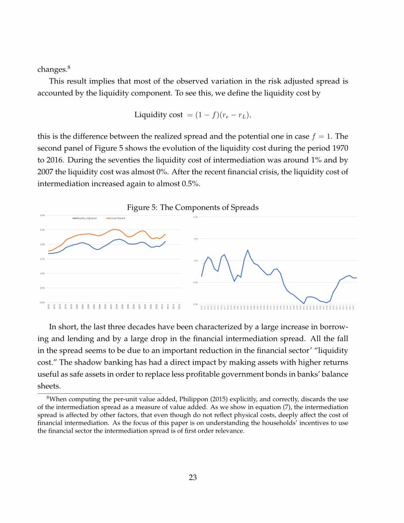
changes.8

This result implies that most of the observed variation in the risk adjusted spread isaccounted by the liquidity component. To see this, we define the liquidity cost by

Liquidity cost = (1− f)(re − rL),

this is the difference between the realized spread and the potential one in case f = 1. Thesecond panel of Figure 5 shows the evolution of the liquidity cost during the period 1970to 2016. During the seventies the liquidity cost of intermediation was around 1% and by2007 the liquidity cost was almost 0%. After the recent financial crisis, the liquidity cost ofintermediation increased again to almost 0.5%.

Figure 5: The Components of Spreads

0.0%

0.5%

1.0%

1.5%

2.0%

2.5%

3.0%

1970

1972

1974

1976

1978

1980

1982

1984

1986

1988

1990

1992

1994

1996

1998

2000

2002

2004

2006

2008

2010

2012

2014

2016

Qualityadjusted LevelBased

0.0%

0.5%

1.0%

1.5%

2.0%

1970

1971

1972

1973

1974

1975

1976

1977

1978

1979

1980

1981

1982

1983

1984

1985

1986

1987

1988

1989

1990

1991

1992

1993

1994

1995

1996

1997

1998

1999

2000

2001

2002

2003

2004

2005

2006

2007

2008

2009

2010

2011

2012

2013

2014

2015

2016

ChartTitle

In short, the last three decades have been characterized by a large increase in borrow-ing and lending and by a large drop in the financial intermediation spread. All the fallin the spread seems to be due to an important reduction in the financial sector’ “liquiditycost.” The shadow banking has had a direct impact by making assets with higher returnsuseful as safe assets in order to replace less profitable government bonds in banks’ balancesheets.

8When computing the per-unit value added, Philippon (2015) explicitly, and correctly, discards the useof the intermediation spread as a measure of value added. As we show in equation (7), the intermediationspread is affected by other factors, that even though do not reflect physical costs, deeply affect the cost offinancial intermediation. As the focus of this paper is on understanding the households’ incentives to usethe financial sector the intermediation spread is of first order relevance.

23

4 Quantitative Assessment of the Model

To perform a counterfactual experiment and decompose the macroeconomic effects of lifeexpectancy (that led to an increase in the demand of safe assets) and the rise of shadowbanking (that led to an increase in the supply of safe assets fueled by the increase in de-mand), we first calibrate the economy to replicate the main aggregates for financial inter-mediation in 1980. Then, we obtain the model’s output for 2007 imposing newly observedlife expectancy and intermediation costs. We analyze what would have happened if theUnited States had to face the demographic transition while forbidding the use of securiti-zation and shadow banking.

4.1 Calibration for 1980

We calibrate the model to replicate yearly data. There are some parameters that are stan-dard in the literature. These are, (i) the discount factor β = 0.99, (ii) capital share θ = 0.3

consistent with a capital income share of output equal to 30%, (iii) labor productivitygrowth, γ = 0.02 and (iv) population growth, η = 0.01.

When choosing the capital depreciation rate, δk, we need to take into account what isthe meaning of capital in our economy. In general, the literature targets a capital-outputratio of 2.7, which is the approximate ratio for the US economy when one focuses onlyon productive capital. In our environment capital encompasses many physical assets thatconstitute wealth for the household, as housing and land. Including these assets the cap-ital output ratio would be around 3.4. Hence, we use as a benchmark δk = 0.0282, whichgenerates such a ratio of 3.4.

Regarding life cycle we assume that agents enter the labor force at age 22. Since theaverage retirement age is 62 we set T = 40. In addition, using the survey of consumerfinances we found that households receive the inheritance on average at age 52. So, weset TI = 30.

In our model 1 − µ represents the proportion of households that directly hold equity.The flow of funds provides information about household’s portfolio choices, showing that28% of American households directly hold equity, which implies that 72% hold equityindirectly. This is µ = 0.72.

In terms of the parameters that determine fiscal policies, we obtain the governmentspending as a fraction of GDP from NIPA tables, g = 0.19. The same way that the cali-bration of K/Y is important for the analysis, because transferring resources across time

24

provides insurance, we need to carefully target the level of government debt. In 1980the ratio of government debt to GDP was around 0.37, while in 2007 the same ratio wasaround 0.62. This in principle implies a larger provision of assets that can be used forinsurance. However, a big part of the increase in government debt is held by foreign in-vestors. Since, the relevant part for our analysis is the domestic availability of these assets,we define the net supply of government debt as total government debt minus debt helpby foreign investors. In 1980 the proportion of public debt held by non-US residents was20%, and set DG/Y = 0.30.

Given these choices there are two parameters left to calibrate: the level of bequestmotives of those households who have bequest motives, α and the fraction of the lastwage that the government transfer for social security after retirement, ssi. As it is notclear what is the best way to calibrate them with exogenous sources of information we setssS = 0 and the other two replicate two important moments, 1) the government debt toGDP ratio of 0.3 in 1980 and, 2) the private debt to GDP ratio of 1 in 1980. In this way weobtain α = 7.5 and ssB = 0.19. To assess the validity of these parameters notice that α of7.5 generates in the model a level of savings consistent with the findings from De Nardi,French, and Jones (2015). Also notice that the calibrated replacement ratio for the socialsecurity system ssB of 19% of the last wage implies in the model a ratio of social securityof 34% of the average wage. The social security administrations provides information formonthly average payments per retired beneficiary, which is around $1.250 per month in2015. Given an average annual wage of $57.000 in 2014, this implies a ratio of 27%, whichis smaller than the ratio generated by the model.9

Finally, there are two important parameters that we will exploit for the counterfactuals:the survival probability after retirement, δ, that captures life expectancy and the spreadbetween borrowing and lending, φ, that captures the role of shadow banking. We startcalibrating δ = 0.08 for 1980, which implies a life expectancy of 12.5 year after retirement.In the counterfactual we decrease this value to δ = 0.06, which implies a life expectancy of16.67 years after retirement, which is the observed value in 2007.10 As shown in Section 3we start calibrating φ = 0.04 for 1980. In the counterfactual exercises we decrease its valueto φ = 0.03, which is the observed value in 2007.

In terms of the performance of the model for those moments that have not been tar-

9Including MEDICARE and MEDICAID, however, this ratio increases and gets close to the implicationsof the model.

10This is slightly conservative since life expectancy is still in a downward path.

25

geted, it generates a ratio of private consumption to GDP of 0.58, very close to the ob-served 0.62 in 1980. The moment that the calibrated model fails to capture well is theamount of inheritance. While the model generates a 4.8% of GDP, most empirical studiesestimate this figure to be around 2.7%. Those empirical estimates, however, abstract frominter-vivos transferees that could be larger in present value than the inheritance.

5 Decomposing Life Expectancy and Shadow Banking.

We now show the counterfactual exercise. The final goal is to decompose the effects of thechange on both life expectancy and intermediation costs on asset accumulation, outputand welfare, from 1980 to 2007.11 We maintain for 2007 a government debt of 30% as aratio of GDP, as the ratio increased to 62% but around 45% of the US federal debt was heldby non-us residents.12 Based on these figures we argue that that provision of governmentbonds during the period under consideration didn’t play an important role in supplyingpublic safe assets.

Since the economic environment affects both the revenue and transfers of the govern-ment, fiscal variables are endogenous but not their composition. Since the main concernfor families in our model is insurance, we focus in the case in which both governmentdebt to GDP ratio and replacement ratio (this is the proportion of wages obtained by thegovernment after retirement) remain constant (roughly as in the data), while the labor taxadjusts to satisfy the government budget constraint. Later, we show the same simulationsbut keeping the labor tax constant and allowing the government debt to change. This lastexercise is helpful to understand the underlying mechanisms affecting our results.

In Table 1, the first column shows the calibration results for 1980. The last columnintroduces the counterfactual when life expectancy increases (captured by a lower δ) andthe agents that sign annuities move from traditional to shadow banks. Because of Propo-sition 1, there exists two levels of search cost, 0 < κ < κ such that if κ ∈ [κ, κ] is optimal forthose agents to choose traditional banks when δ = 0.08 and shadow banks when δ = 0.06.Due to the move from traditional to shadow banks, the intermediation spread falls from

11As over time the population growth rate has shown important changes, increasing to 1.4% in 1992, andthen falling to 0.7% in 2011, in this counterfactual for 2007 we set η = 0.007. The population growth ratehas first order effects, due to demographic accounting, to match the level of government debt and aggregatebequest in 2007, but its change have little effect on the observes changes in financial intermediation.

12See http://www.treasury.gov/resource-center/data-chart-center/tic/Pages/ticsec2.aspx. See alsoBertaut et al. (2012) for a detailed discussion about the international saving glut in the US economy.

26

φ = 0.04 to φ = 0.03, as we observe in the data and model in Section 3.Comparing the first and last columns, in which we allow both an increase in life ex-

pectancy and a reduction in spreads as observed in the data, the model generates a largeincrease in the output steady-state level (of around 6%), an increase in capital output ratio(from 3.4 to 3.9) and a large increase in households’ total financial assets (from 1.3 to 1.96).While the data counterpart of the first two figures are difficult to observe, we use TableL100 of the flow of funds to measure the increase of households financial assets, a proxyfor debt instruments. Subtracting from the total domestic non-financial assets (Line 1, Ta-ble L100) the corporate equity (Line 16, Table L100) and the equity on non-corporate busi-nesses (Line 23, Table L100), we obtain a proxy for the net-worth of households that followstrategy B. In the US economy financial assets grew from 1.36 GDP to 2.33GDP, which isvery close to the model’s predictions. Finally, the model’s prediction of the change in thenew amount intermediated, measured by the Household Debt to GDP ratio, accounts formore than 90% of the observed change.

Now we can decompose the effects of the increase in life expectancy and the decline inintermediation costs by suppressing one at a time. The second column of Table 1 showsthe counterfactual without shadow banks. We compute the model with life expectancyincreasing in the same magnitude as observed in the data, but assuming that κ > κ, sothat the move to shadow banking does not happen. Without the move to shadow bankingthe increase in capital output ratio and steady state output would have been around 60%of the total increase with the presence of shadow banking (capital output ratio increasedfrom 3.4 to 3.7 instead of to 3.9 while output increased from 1 to 1.034 instead of to 1.062).The increase in retirement needs generates a permanent increase of GDP of almost 3%instead of 6% with shadow banks. Also, absent shadow banking we would have observeda small change in the net worth held by agents as debt products in terms of GDP (from 1.3to 1.4 instead of to 1.96) and household debt over GDP (from 1 to 1.1 instead of to 1.66).Finally, an increase in retirement needs without an improvement in intermediation costswould increase the demand for safe assets, which generates a reduction in their return (rdeclines from 0.020 to 0.013). Still, since there are more funds channeled to investmentopportunities the equity return declines (re declines from 0.060 to 0.053).

Finally, the third column of Table 1 is a thought experiment without an increase inlife expectancy, where we assume that κ falls below the lower bound κ, reducing inter-mediation cost, even though life expectancy remains in the levels of 1980. To make the

27

Table 1: Counterfactual to 2007 (Fixed DG)

1980 Larger δ Same δ δ & φ changeEconomy Benchmark κ > κ κ < κ κ ∈ [κ, κ]Interm. Cost (φ) 4% 4% 3% 3%Survival prob. (δ) 0.08 0.06 0.08 0.06

Interest RatesBorrowing Rate (r) 0.020 0.013 0.025 0.018Lending Rate (re) 0.060 0.053 0.055 0.048

National AccountsOutput 1.00 1.034 1.025 1.062Capital output ratio 3.40 3.70 3.60 3.91

Net WorthTotal 3.70 3.97 3.90 4.21

Equity (Plan S) 2.40 2.57 2.12 2.25Debt (Plan B) 1.30 1.40 1.78 1.96Data (FF: Table L100) 1.36 2.33

Bequest/Y 0.048 0.048 0.040 0.040Government Debt/Y 0.30 0.30 0.30 0.30Households Debt/GDP 1.00 1.10 1.48 1.66Data (FF: Table D3) 1.00 1.73

Change on welfare at birth - - 0.3% 0.4%Plan B - - 2.5% 2.8%Plan S - - -4.3% -4.8%

exercise comparable to the fourth column, we assume that the intermediation costs de-cline in the same magnitude as observed in the data in 2007. In essence, this exerciseshows what would have happened in our model with shadow banking but no increase inlife expectancy and then extra needs for retirement since 1980. In this case, the increasein capital output ratio and steady state output would have been around 40% of the totalincrease with the higher retirement needs (capital output ratio increased from 3.4 to 3.6instead of to 3.9 while output increased from 1 to 1.025 instead of to 1.062). That is, thearrival of shadow banking without an increase in demand of financial assets for higher

28

life expectancy would have generated a permanent increase in GDP level of almost 3%instead of 6%. Also, we would have observed a large change in the net worth held byagents in terms of GDP (from 1.3 to 1.78 instead of to 1.96) and household debt over GDP(from 1 to 1.48 instead of to 1.66). Finally, a reduction in intermediation costs increase thesupply of funds, inducing an increase in the return of safe assets (r increases from 0.020 to0.025). Still, since there are more funds channeled to investment opportunities the equityreturn still declines (re declines from 0.060 to 0.055).

The different effects of retirement needs and shadow banking on asset returns empha-size the relevance of modelling both demand and supply of the asset markets, as pointedout by Justiniano, Primiceri, and Tambalotti (2013) and Justiniano, Primiceri, and Tam-balotti (2015), who relate the credit boom in the first half of 2000s to the international sav-ing glut. They stressed the fact that the fall in interest rates was due to the influx of foreignfunds. From this point of view, our paper can be understood as accounting for the con-tribution of a “domestic saving glut” generated by longer living U.S. residents, which hasbeen largely ignored in the literature. In particular, Justiniano, Primiceri, and Tambalotti(2013) argue that between one fourth and one third of the increase in the U.S. householddebt can be accounted by the international saving glut. The domestic saving glut togetherwith the fall in the liquidity cost can account for all of the increase in household debt.13

Remark on Welfare EffectsWhen there are changes to “preferences” (in our case life expectancy, δ, changes) af-

fecting the computation of present values, comparisons across experiments become hardto interpret in terms of welfare. If in two experiments δ is the same, this is no longer aproblem though. When this is the case, we use the consumption equivalent change nec-essary to make a household indifferent between the two alternatives. With logarithmicutility, as we have assumed, the calculations are quite simple.

Let C = {ct, bt}∞t=0 be the sequence of consumption and bequest for an agent at birth be-fore a change on the economy and C = {ct, bt}∞t=0 the analogous sequence after the change.We define the consumption equivalent parameter λ as the constant proportional changein every period allocation that makes the consumer indifferent between the two alterna-tives. That is, λ solves

∑∞t=0((1 − δt)β)tu((1 + λ)ct, (1 + λ)bt) =

∑∞t=0((1 − δt)β)tu(ct, bt).

Thus, if λ is positive the consumer benefits from the change while if it is negative the con-sumer is worse off. Since preferences are logarithmic. The above equation can be written

13As we mention in Section 4.1 most of the foreign funds went into government bonds. Thus, the directeffect of the international saving glut is likely small.

29

as∑∞

t=0((1−δt)β)t log(1+λ)+∑∞

t=0((1−δt)β)tu(ct, bt) =∑∞

t=0((1−δt)β)tu(ct, bt). Let U0(C)

be the utility at birth, then λ satisfies:[1− βT+1

1− β+

βT

1− β(1− δ)

]log(1 + λ) = U0(C)− U0(C)

λ = exp

[−1− βT+1

1− β− βT

1− β(1− δ)

]exp [U0(C)− U0(C)]− 1

From now on, the change on welfare is expressed in terms of 100λ%.Comparing column 1 and 3, which are computations based on the same δ = 0.08 but

lower intermediations costs due to shadow banking, we observe an increase in welfare of0.3%. It is interesting to notice that the increase is due to a big consumption equivalent in-crease of 2.5% for the annuity type (which are almost 70% of the agents) while the welfareof the equity type decreases drastically by 4.3%.

The increase on welfare is higher (by 0.4%) when comparing columns 2 and 4, based ona higher life expectancy of δ = 0.06. Again, the big gain in welfare comes from the bank-financing agents who benefit from the more efficient financial system in the economy by2.8%, while self-financing agents get worse off, experiencing a lost of 4.3% of terms oflife-time consumption. Notice that the relatively higher average welfare gain is due to thehigher gain experienced by bank-financing agents.

Remark on allowing Government Debt/GDP to changeIn the previous simulations we maintained DG fix. In Table 2 we consider alternative

scenarios for DG. The first column just replicates the calibration in Table ?? while thesecond column replicates the counterfactual for 2007 when allowing both retirement needsand intermediation costs to vary (the last column of Table 1). The third column showswhat would the equilibrium have been if the life expectancy had increased, the spreadhad decreased to 3% and the government were allowed to freely choose the level of debtwithout changing either taxes or transfers. In this case, the government becomes a netsaver (given constant taxes and larger expenses due to the social security system, the onlyway to finance its expenses is to accumulate assets and to use the proceeds to compensatethe shortfall of revenue). As the government stop providing public safe assets and startdemanding them, there is a reduction in interest rates (r and re drops by 0.001). Thisimplies that both the capital output ratio and the steady state output increase further thatin the case of fixed DG (almost 20% more in both cases). In addition, the household debt

30

Table 2: Counterfactual to 2007 (alternative DG)

1980 2007 Free All DG

Economy Benchmark Calibration DG DomesticInterm. Cost (φ) 4% 3% 3% 3%Survival prob. (δ) 0.08 0.06 0.06 0.06

Interest RatesBorrowing Rate (r) 0.020 0.018 0.017 0.020Lending Rate (re) 0.060 0.048 0.047 0.050

National AccountsOutput 1.00 1.06 1.07 1.05Capital output ratio 3.40 3.91 4.00 3.83

Net WorthTotal 3.70 4.21 3.96 4.45

Equity (Plan S) 2.40 2.25 2.16 2.34Debt (Plan B) 1.30 1.96 1.80 2.11Data (FF: Table L100) 1.36 2.33

Bequest/Y 0.048 0.040 0.038 0.042Government Debt/Y 0.30 0.30 -0.04 0.62Households Debt/GDP 1.00 1.66 1.84 1.49Data (FF: Table D3) 1.00 1.73

explode to 1.84 GDP, almost 30% more than in the case of fixed DG.Finally, the last column assumes that the debt to GDP ratio moves from 0.3, as in 1980,

to 0.62, which it would be domestic supply of government bonds in 2007 if the foreignnations would not hold any U.S. treasuries (see Section 4.1 ). The difference betweenthis equilibrium and the observed in 2007 inform us about the indirect effect of the in-ternational saving glut on the US financial intermediation system. The main effect is anincrease in the supply of public safe assets that maintain r at levels before the increase inlife expectancy even though intermediation costs decline. This induces a decline of house-hold debt to GDP ratio with respect to the case in which there is no global saving glut, to1.49GDP instead to 1.66GDP. This result implies that the international demand for U.S.treasuries would account for around 25% of the generated increased in the US household

31

debt. This number is very close to the interval provided by Justiniano, Primiceri, andTambalotti (2013) for the contribution of the international saving glut to the credit boomin the 2000. However, in our setup the channel is different. There is no direct supplyof foreign funds (lenders) generating incentives that stimulates household’s borrowing.Instead, the foreign demand for U.S. treasuries crowds out the domestic demand for safeassets. Second, GDP would have increased less without a foreign saving glut.

5.1 Transitions

Since it can take many years for an economy to converge to a new steady state, comparingtwo steady states may not be the best way to assess the impact of a life expectancy changein the economy from 1980 to 2007. In this section we show that the convergency is indeedquite fast: by the year 2010 most of the increase in debt, around 90%, has already hap-pened. We also show that cyclical movements of economic activity play an important roleaccommodating the slow grow in debt during the early 80’s and the subsequent speedingup in private indebtedness during the 2000’s.

The computation of the transition, however, presents several challenges. First, at thetime of the shock there is a distribution of agents indexed by age and assets. Who is af-fected when the death probability shock happens in 1980? In what follows, we assumethat retired agents, at the moment of the shock, remain with the initial surviving probabil-ity δ = 0.08, while the surviving probability for all working-age agents jump to δ = 0.06.Second, some agents were already in an annuity contract. What happens what those con-tracts? We assume that after the shock all the existing contracts are renegotiated to takeinto account the new survival probability. Third, what happens with the government bud-get? We assume that the lump-sum transfers remain at the same absolute value as beforethe shock and that the government still follows a policy to maintain the debt to outputratio constant and equal to 0.3. As a result, the labor tax has to adjust during the tran-sition to keep the government’s budget balanced. Finally, what happens with retirementpayments? We assume that for those already retired in 1980, these payments remain atthe same level that were contracted before the shock.

In Figure 6 we show the transition dynamics of a shock that reduces δ from 0.08 to 0.06

and reduces φ from 0.03 to 0.02, while in Table 3 we present the values corresponding tothe figure. In panel a) of the figure we see that immediately after the shock the spread falls.

32

Figure 6: Transition Dynamics: constant TFP

1980 1990 2000 2010 2020

0.025

0.03

0.035

0.04

0.04

0.05

0.06

Lending RateBorrowing Rate

(a) Interest Rates

1980 1990 2000 2010 2020

1

1.02

1.04

1.06

1.08

1.1

(b) Output

1980 1990 2000 2010 2020

1.5

2

2.2

2.4

2.6

Type BType S

(c) Aggregate Assets/Output

1980 1990 2000 2010 2020

0.8

1

1.2

1.4

1.6

(d) Household Debt/Output

Figure 2: Transition Dynamics - Constant TFP

2

Table 3: Transition values

Variable/year 1980 1985 1990 1995 2000 2005 2010 2015K/Y 3.399 3.528 3.648 3.735 3.796 3.838 3.866 3.883Y 1.000 1.016 1.031 1.041 1.049 1.053 1.057 1.059Type B Net worth 1.306 1.440 1.570 1.669 1.746 1.804 1.848 1.880Type S Net worth 2.397 2.391 2.382 2.369 2.354 2.337 2.321 2.306Total Fin. Assets 1.609 1.743 1.873 1.972 2.049 2.107 2.151 2.184Gov. Debt/GDP 0.303 0.476 0.508 0.500 0.325 0.332 0.303 0.303Private Debt/GDP 1.003 1.137 1.266 1.366 1.442 1.501 1.545 1.577

After the shock, both interest rates continuously decline until they reach the new steadystate. The non-monotone convergency of the lending rate is because with the new lifeexpectancy the capital stock is low respect to its desired value. Thus, the return on savings

33

increases and slowly converges to the new, now lower, level of returns. This effect can beseen in the increasing pattern for the net worth of bank-insuring households in panel c).Also, in panel c) we see that the net worth of self-insuring households continuously fall, inspite of an increasing on the capital stock, as they increase the leverage ratio. As a result, inpanel d) the household debt increase from 1GDP in 1980 to about 1.54 by 2007, almost 85%of the difference between steady states. In this dimension, the fall in the intermediationcost plays an important role. If the intermediation cost is kept constant at the 1980 levels,self-insuring households’ net worth would have increased instead of falling, but in anycase the household debt would have increased. Finally, in panel b) we see that by 2007 theoutput is very close to the new steady state.

Figure 7: Transition Dynamics: observed TFP

1980 1990 2000 2010 20200.02

0.025

0.03

0.035

0.04

0.045

0.04

0.045

0.05

0.055

0.06

0.065Lending RateBorrowing Rate

(a) Interest Rates

1980 1990 2000 2010 2020

1

1.02

1.04

1.06

1.08

1.1

(b) Output

1980 1990 2000 2010 2020

1.5

2

2.2

2.4

2.6

Type BType S

(c) Aggregate Assets/Output

1980 1990 2000 2010 2020

0.8

1

1.2

1.4

1.6

(d) Household Debt/Output

Figure 1: Transition Dynamics - Observed TFP

1

Notice that the increase on private debt starts immediately after the shock, while in theUS economy the accumulation of debt starts later. To that end we compute the transitionpath using the actual path for TFP (measured by the Solow residual) instead of fixing

34

A = 1 as in the previous simulations. In Figure 7 we show that the recessions in early 80’sand early 90’s slow down the convergence in the 80’s, to speed up again in the secondhalf of the 90’s. Also notice that the monotone declining rate of the interest rate is mostlyunaffected by the changes in the TFP, while the output and private debt are slightly abovethe figures computed in Figure 6.

6 On the Costs and Benefits of Shadow Banking

In this paper we have abstracted from the cost of shadow banking. The great recessionis an example of how big this costs can be if indeed it was partly generated by a collapsein securitization and most instruments heavily used to provide liquidity at a lower costin shadow banking activities. Using a methodology proposed by Luttrell, Atkinson, andRosenblum (2013) and later expanded by Ball (2014) and Fernald (2014) that compares thepotential output computed by the Congressional Budget Office (CBO) and the realizedoutput we computed that the great recession generated a lost of GDP, in present value, of23% of 2007 GDP. In Figure 8, this is the discounted value in 2007 of the difference betweenthe dotted back line and the dashed red realized output after 2007.14

A natural question arises if shadow banking was responsible for the crisis, was it worthit? Was the contribution of shadow banking large enough to compensate the observedcost? The first approach to the answer can be found in Table 1, which can be used tocompute the present value of its contribution to generate income. Since, shadow bankinggenerates a permanent increase of output equivalent to 2.8% per year in the stationaryequilibrium (1.062-1.034, see the second and forth columns of Table 1), discounting the fu-ture (growing) stream of income using the risk free interest rate we obtain a present valueof around 3.3GDP of 2007. Nonetheless, this would be the gains from shadow bankingin the long run absent any crisis. This is not, however, the correct number to comparewith the losses after the crisis, in particular because previous to 2007 the economy was ina transition, not in the stationary equilibrium.

In order to compare meaningfully the benefits and cost of shadow banking surround-ing the recent crisis, we compute a benchmark economy without shadow banks, this iswithout the potential gains from lower spreads but also without the cost of a crisis. To

14This is lower than the estimation in these papers that range from 40% to 90% of 2007 GDP, mainlybecause the CBO has revised down potential output in the last two years. For a detailed explanation aboutthe calculations see the staff report Atkinson, Luttrell, and Rosenblum (2013).

35

perform this counterfactual we assume κ > κ, so that after the increase in life expectancyindividuals just keep choosing traditional banks and the spreads were at the 1980 level of3%. We use the gap in output from the counterfactual and we extrapolate it to the realizedGDP until 2007.

In this counterfactual there is no shadow banking previous to 2007, but we need toextend it such that there is no crisis after that. It is challenging to compute the potentialoutput in the counterfactual as we should take a stand on how productivity and othervariables would have evolved in the economy without a crisis. For this reason we willconservatively assume that the economy keeps increasing at the average growth levelsince 2007. This counterfactual is the blue solid line of Figure 8 until 2007 and the dashed-dotted grey line after 2007.

Figure 8: The costs and benefits of shadow banking

6400

8400

10400

12400

14400

16400

1980 1985 1990 1995 2000 2005 2010 2015 2020

NeverShadow Banking

ActualGDPandforecast(after2016)

PotentialGDP(CBO)

AlternativePotential

With our counterfactual we can now compute the gains from shadow banking before2007 and its losses after 2007. The present value of the gap between the benchmark andthe realized output from 1980 to 2007 (which, as we discussed, corresponds to a transition

36

period) represents a 47% of 2007 GDP. The gap between the benchmark and the realizedoutput from 2007 to 2020 represents a 16% of 2007 GDP. The comparison between thesetwo numbers delivers a net gain from shadow banking, even after assigning all the cost ofthe crisis to it, of 30% of 2007 GDP.

Note that this cost based on our counterfactual is below the 23% that the literature hasproposed taking as benchmark the potential output by the CBO. The reason is that theinitial level of that potential output is the realized output before the crisis, which accord-ing to our model was high initially exactly because shadow banking was instrumental inincreasing output. After the crisis, shadow banking activities collapsed and regulationhas been enacted that restricted its resurgence. This may be the reason the CBO reducedthe potential output estimation and why our counterfactual converges to their potentialoutput estimation in 2017. In other words, measuring the cost of a financial crisis usingpotential output may be correct in terms of consequences for forgone income, but inter-preting it as a cost of shadow banking is misleading as it could be indeed pointing to itsvalue instead.

7 Conclusions

The recent discussion, both in academic and policy circles, about the demand of safe assetsand its macroeconomic effects has focused on the “saving glut” from foreign countries. Atthe same time, the recent discussion about the role of shadow banking has focused on itspervasive effects on triggering painful crises. In this paper we argue that these two dis-cussions are intimately related. While the higher foreign demand of safe assets seems tohave been accommodated by an increase in government debt, the higher domestic de-mand of safe assets triggered by an increase in life expectancy has pushed an endogenousincrease in the supply of safe assets by the private sector, more specifically securitizationand shadow banking. We have explored quantitatively the individual roles of higher lifeexpectancy and the rise of shadow banking on the accumulation of financial assets, privatedebt, output and welfare.

We show that a calibrated model with an increase in the demand of safe assets forretirement needs and shadow banking that reduces the cost of financial intermediationaccommodates well the large increase in asset accumulation and output experienced bythe United States since 1980. We find that in the absence of shadow banking assets wouldnot have increased, while the capital-output ratio and output would have increased only

37

half of what they did.Our approach allows us to compute a counterfactual without shadow banks and we

have shown that the gains from 1980 to 2007 of operating with shadow banking was of47% of 2007 GDP. Further, even if we assume shadow banking was the sole responsible forthe recent crisis and the whole great recession, its cost is of the order of 16% of 2007 GDP.In other words, our model suggest that there were net gains of having shadow bankseven if it were true that it single handedly generated the great recession. These resultsare relevant in the discussion about the regulation of the banking system. Even thoughavoiding shadow banks or certain financial innovations, such as securitization, may havebenefits in terms of reducing the likelihood and magnitude of financial crises, we showthat it is also costly in terms of choking-off output.

38

References

Alvarez, Fernando, Luigi Guiso, and Francesco Lippi. 2012. “Durable Consumptionand Asset Management with Transaction and Observation Costs.” American EconomicReview 102 (5): 2272–2300 (May).

Atkinson, Tyler, David Luttrell, and Harvey Rosenblum. 2013, July. “How bad wasit? The costs and consequences of the 2007–09 financial crisis.” Technical Report 20,Federal Reserve Bank of Dallas.

Ball, Laurence. 2014. “Long-Term Damage from the Great Recession in OECD Coun-tries.” NBER Working Paper 20185.

Begenau, Juliane, and TIm Landvoigt. 2017. “Financial Regulation in a QuantitativeModel of the Modern Banking System.” working Paper, Stanford University.

Bertaut, Carol, Laurie Pounder DeMarco, Steven Kamin, and Ralph Tryon. 2012. “ABSinflows to the United States and the global financial crisis.” Journal of InternationalEconomics 88 (2): 219–234.

Bloom, David E., David Canning, Richard K. Mansfield, and Michael Moore. 2007. “De-mographic change, social security systems, and savings.” Journal of Monetary Eco-nomics 54 (1): 92 – 114. Carnegie-Rochester Conference Series on Public Policy: Eco-nomic Consequences of Demographic Change in a Global Economy April 21-22, 2006.

Bloom, David E., David Canning, and Michael Moore. 2014. “Optimal Retirement withIncreasing Longevity.” Scandinavian Journal of Economics 116 (3): 838–858 (07).

Caballero, Ricardo. 2010. “A Caricature (Model) of the World Economy.” Working Paper,MIT.

Caballero, Ricardo, Emmanuel Farhi, and Pierre-Olivier Gourinchas. 2016. “Global Im-balances and Currency Wars at the ZLB.” Working Paper, MIT.

Carvalho, Carlos, Andrea Ferrero, and Fernanda Nechio. 2016. “Demographics and realinterest rates: Inspecting the mechanism.” European Economic Review 88 (C): 208–226.

Corvae, Dean, and Pablo D’erasmo. 2013. “A Quantitative Model of Banking IndustryDynamics.” Manuscript.

Costa, Dora L. 1998. “The Evolution of Retirement: Summary of a Research Project.” TheAmerican Economic Review 88 (2): 232–236.

De Nardi, Mariacristina, Eric French, and John Jones. 2009. “Life Expectancy and OldAge Savings.” American Economic Review, Papers and Proceedings 99 (2): 110–115.

. 2010. “Why Do the Elderly Save? The Role of Medical Expenses.” Journal ofPolitical Economy 118:39–75.

. 2015. “Savings After Retirement: A Survey.” NBER working paper no. 21268.

39

Fagereng, Andreas, Charles Gottlieb, and Luigi Guiso. 2017. “Asset Market Participa-tion and Portfolio Choice over the Life-Cycle.” The Journal of Finance 72 (2): 705–750(March).

Farhi, Emmanuel, and Jean Tirole. 2017. “Shadow Banking and the Four Pillars of Tradi-tional Financial Intermediation.” Working Paper, Havard University.

Fernald, John. 2014. “Productivity and Potential Output Before, During and After theGreat Recession.” Federal Reserve Bank of San Francisco Working Paper 2014-15.

Gale, William, and John Karl Scholz. 1994. “Intergenerational transfers and the accumu-lation of wealth.” Journal of Economic Perspectives 8 (4): 145–160.

Gorton, Gary, and Guillermo Ordonez. 2014. “Collateral Crises.” American EconomicReview 104 (2): 343–378.

Gustman, Alan, and Thomas Steinmeier. 1999. “Effects of pensions on savings: Analysiswith data from the health and retirement study.” Carnegie-Rochester Conference Serieson Public Policy, Volume 50. Elsevier, 271–324.

Harris, Milton, Christian Opp, and Marcus Opp. 2014. “Higher Capital Requirements,Safer Banks? Macroprudential Regulation in a Competitive Financial System.” Work-ing Paper, Wharton School.

Justiniano, Alejandro, Giorgio Primiceri, and Andrea Tambalotti. 2013. “The Effects ofthe Saving and Banking Glut on the U.S. Economy.” In NBER International Seminar onMacroeconomics 2013, NBER Chapters, 52–67. National Bureau of Economic Research,Inc.

. 2015. “Credit Supply and the Housing Boom.” Manuscript.

Kotlikoff, Laurence J., and Lawrence H. Summers. 1981. “The Role of IntergenerationalTransfers in Aggregate Capital Accumulation.” Journal of Political Economy, pp. 706–732.

Lockwood, Lee. 2012. “Bequest Motives and the Annuity Puzzle.” Review of EconomicDynamics 15 (2): 706–732.

. 2015. “Incidental Bequests: Bequest Motives and the Choice to Self-Insure Late-Life Risks.” Manuscript.

Luttrell, David, Tyler Atkinson, and Harvey Rosenblum. 2013. “Assessing the costs andconsequences of the 2007 - 09 financial crisis and its aftermath.” Economic Letter, vol. 8(Septiembre).

Mankiw, N. Gregory, and Stephen Zeldes. 1991. “The consumption of stockholders andnonstockholders.” Journal of Financial Economics 29 (1): 97–112.

Mehra, Rajnish, Facundo Piguillem, and Edward Prescott. 2011. “Costly Financial Inter-mediation in Neoclassical Growth Theory.” Quantitative Economics 2 (1): 1–36.

Moreira, Alan, and Alexi Savov. 2015. “The Macroeconomics of Shadow Banking.” Work-ing Paper, Yale University.

40

Ordonez, Guillermo. 2014. “Confidence Banking and Strategic Default.” Working Paper,University of Pennsylvania.

. 2017. “Sustainable Shadow Banking.” American Economic Journal: Macroeco-nomics. Forthcoming.

Philippon, Thomas. 2015. “Has the US Finance Industry Become Less Efficient? On theTheory and Measurement of Financial Intermediation.” American Economic Review105 (4): 1408–38.

Plantin, Guillaume. 2015. “Shadow Banking and Bank Capital Regulation.” Review ofFinancial Studies 28 (1): 146–175.

Wolff, Edward. 2004. “Changes in household wealth in the 1980s and 1990s in the U.S.”Levy Economics Institute Working Paper 407.

41