i

Erasmus University Rotterdam

MSc in Maritime Economics and Logistics

2017/2018

Assessing potential market share and container flows of short sea shipping as an alternative

transportation mode: The case of the Northern Java’s route, Jakarta – Surabaya corridor,

Indonesia

By

Muhammad L. Hakim

copyright © Muhammad L. Hakim

ii

Acknowledgments

Alhamdulillah, all praises to Allah for His blessings for a year full of joy and happiness in the one of the biggest port cities in the world, Rotterdam. To my parents and family, all my achievements and life will be dedicated, without them, I was nothing and now I am still nothing compared to their dedication to me. A one-year master course is probably not enough for us, but no, no, I don’t want to do it again, seriously. Anyway, you guys did an excellent job, the MEL team, especially Martha.

I would like to thank my first Dutch friend who surprisingly knows Indonesian maritime industry so much as well as the only one Dutch who unexpectedly mentioned my previous company where I worked before, my first supervisor, Dr. Simme Veldman who has inspired me to write this thesis’s topic, even though he couldn’t continue to supervise me because of his health issues, praying that he gets better soon and experience the joys of being healthy again.

A special credit is also given to my thesis supervisor, drs. Ted Welton, who always gives me motivation and additional energy during the thesis period and shockingly I finished my thesis earlier than what I thought before. I am very grateful to have the best former colleagues who always support me since the beginning of the course until my thesis period finished, Pak Adi Dharma and Mas Setyo Wicaksono. Also thanks to the beloved classmates, especially Indonesian students who have supported each other during the tough period. For all my friends in Rotterdam and Indonesia, I would like to say thank you! I promise you that we will meet again at the higher level of life. See you soon, Rotterdam!

iii

Abstract

The Indonesian national roadway, called the Northern Java’s route, has been experiencing various disputed issues for many years. The roadway is situated in the north coast of Java island, which is one of the most densely populated islands in the world as it stretches between the two greatest cities in Indonesia, Jakarta, and Surabaya. Therefore, it is not surprising that the cargo traffic between the cities reaches up to 1.7 million TEUs container annually, however, that number is almost as big as the national cargo flows. The primary issue now is more than 90% of the cargo flows are transported via roadway which severely results in some problematic issues such as congestions, air pollutions, noise pollutions and high maintenance costs. Additionally, the road capacity is no longer enough to provide the transportation demands. An approach is proposed by the idea of the utilization of national maritime potential namely short sea shipping. The concept is simply transporting cargo by vessel or water-based vehicles among the short-distance regions in which Jakarta – Surabaya distance is applied. Short sea shipping has globally become an effective approach to solve the transportation problems. Some countries, for instances, US, EU, Canada, and Vietnam, have been implementing this method to solve their national transportation issues. Thus, this research aims to obtain the figure of estimated market share and transported container once short sea shipping is being employed along the Northern Java’ coast. The figures are obtained by conducting a modal split model given the utility functions and the stated preferences. Two attributes are attached such as operational cost and transporting time to generate the utility functions. Meanwhile, stated preferences by freight forwarders are counted as the coefficient of the utility function. It is deduced that short sea shipping obtains 30.4% shares or approximately 523.023 TEU containers to transport along the route of Jakarta – Surabaya and the other way around. However, this market share’s value increases more than 20% from the initial shares, meaning that it should be anticipated by the port companies, shipping companies, and even the local government in order to constantly provide a sufficient container flow.

iv

Table of Contents

Acknowledgments .......................................................................................................... ii

Abstract ......................................................................................................................... iii

Table of Contents ........................................................................................................... iv

List of Tables .................................................................................................................. vi

List of Figures ............................................................................................................... viii

List of Abbreviations ...................................................................................................... ix

Chapter 1 Introduction .................................................................................................... 1

1.1. Research objectives.................................................................................................. 2

1.2. Research question and sub-research questions ...................................................... 3

1.3. Research design and methodology .......................................................................... 3

1.4. Thesis structure ........................................................................................................ 4

Chapter 2 Short sea shipping and Indonesian supply chain and logistics ........................... 6

2.1. Short sea shipping as an alternative transportation ..................................................... 6

2.1.1. Definition of short sea shipping ............................................................................. 6

2.1.2. Development and Implementation of short sea shipping ..................................... 7

2.1.3. Fundamental reasons for conducting short sea shipping ...................................... 8

2.1.4. Intermodal container transport ........................................................................... 11

2.2. Overview of short sea shipping, supply chain, and logistics flows in Indonesia ......... 11

2.2.1. Indonesian logistics networks .............................................................................. 11

2.2.2. The Northern Java’s route .................................................................................... 13

2.2.3. Available transportation modes across the north coast ...................................... 15

2.2.4. The government's intention in the domestic maritime industry. ........................ 20

2.3. Conclusion ................................................................................................................... 20

Chapter 3 Research methodology and data .................................................................... 22

3.1. Modal split model.................................................................................................. 22

3.2. Stated preference analysis for coefficient of utility function ................................ 26

3.3. Operational cost and delivery time analysis .......................................................... 27

3.3.1. Truck transportation mode ............................................................................ 31

3.3.2. Multimodal rail transport ............................................................................... 34

3.3.3. Multimodal sea transport .............................................................................. 35

3.4. Data collection ....................................................................................................... 43

v

3.5. Data analysis .......................................................................................................... 43

3.6. Conclusion .............................................................................................................. 44

Chapter 4 Result and analysis ........................................................................................ 45

4.1. Estimated operational cost .................................................................................... 45

4.2. Estimated travel time ............................................................................................. 47

4.3. Estimated market share ......................................................................................... 49

4.4. Potential container flows ....................................................................................... 52

4.5. Conclusion and key findings ................................................................................... 53

Chapter 5 Conclusion .................................................................................................... 57

5.1. Answers to the research questions ........................................................................ 57

5.2. Advice ..................................................................................................................... 57

5.3. Limitations of research and suggestions for further study .................................... 59

References .................................................................................................................... 61

vi

List of Tables

Table 1. Tariff for a TEU container from Jakarta to Surabaya or vice versa .............. 16

Table 2. Container transported by three shipping liners from Jakarta to Surabaya. 18

Table 3. Freight rate offered by Meratus Line (2018). ................................................... 19

Table 4. Current available transportation modes. .......................................................... 21

Table 5. The coefficient of the utility function. ................................................................. 27

Table 6. Locations around Tanjung Priok Port Jakarta. ................................................ 27

Table 7. Locations around Tanjung Perak Port Surabaya. ........................................... 28

Table 8. Transshipment point for railway and vessel. ................................................... 29

Table 9. Transport Distance from West to East.............................................................. 30

Table 10. Transport Distance from East to West. .......................................................... 31

Table 11. Component of Trucking Cost. .......................................................................... 32

Table 12. Trucking Cost Simulation. ................................................................................ 32

Table 13. Estimated Cargo Volume and Vessel size. ................................................... 36

Table 14. Break down of Vessel Travel Time. ................................................................ 38

Table 15. Estimated Bunker Cost. .................................................................................... 39

Table 16. Estimated Other operating costs. .................................................................... 40

Table 17. Estimated Capital Costs. .................................................................................. 40

Table 18. Port charges in two different ports. ................................................................. 41

Table 19. Cargo handling charges in two different terminals. ...................................... 41

Table 20. The total cost of short sea shipping. ............................................................... 42

Table 21. Operational costs for the west-to-east route. ................................................ 46

Table 22. Operational costs for the east-to-west route. ................................................ 47

Table 23. Average estimated cost. ................................................................................... 47

vii

Table 24. Travel time for the west-to-east route. ............................................................ 48

Table 25. Travel time for the east-to-west route. ............................................................ 49

Table 26. Average estimated travel time. ........................................................................ 49

Table 27. Market share for the west-to-east route. ........................................................ 51

Table 28. Market share for the east-to-west route. ........................................................ 51

Table 29. Market share in certain origin-destination points. ......................................... 52

Table 30. Average market share among the modes...................................................... 52

Table 31. Container Flows in Jakarta – Surabaya Corridor for three different options.

................................................................................................................................................ 52

Table 32. Container Flows in Jakarta – Surabaya Corridor for three different options.

................................................................................................................................................ 54

Table 33. Comparison of current condition and estimated travel time. ....................... 54

viii

List of Figures

Figure 1. Map of Java Island and the two biggest cities, Jakarta and Surabaya. ....... 1

Figure 2. Research methodological flow. .......................................................................... 4

Figure 3. Fuel consumption and CO2 emission for three transportation modes. ......... 9

Figure 4. Logistics Performance Index (LPI) for ASEAN countries. ............................ 12

Figure 5. Northern Java’s route......................................................................................... 13

Figure 6. Commodity shares between the routes. ......................................................... 14

Figure 7. Market share of transportation mode. ............................................................. 14

Figure 8. Three different routes provided along Java island. ....................................... 16

Figure 9. Railway network in Java island. ....................................................................... 17

Figure 10. Average port dwelling time among ASEAN countries. ............................... 19

Figure 11. Supply and Demand Interaction. .................................................................... 23

Figure 12. Probability Density Function. .......................................................................... 24

Figure 13. Cumulative Distribution Function with the same variance and mean. ..... 24

Figure 14. Locations around Tanjung Priok Port Jakarta.............................................. 28

Figure 15. Locations around Tanjung Perak Port Surabaya. ....................................... 28

Figure 16. Origin and destination simulation networks. ................................................ 29

Figure 17. Multimodal Rail Transport Illustration. ........................................................... 34

Figure 18. Multimodal Sea Transport Illustration. .......................................................... 35

Figure 19. Vessel operational cost and travel time analysis. ....................................... 36

Figure 20. The proportion of short sea shipping cost. ................................................... 42

Figure 21. Current and potential market shares. ............................................................ 55

Figure 22. Initial and potential additional container flows. ............................................ 56

ix

List of Abbreviations

ASEAN Association of Southeast Asian Nations

BPS The national data center

CRF capital recovery factor

CY Container Yard

DWT Deadweight

g/tkm Gram per Ton Kilometers

GDP Gross Domestic Product

GT Gross Tonnage

HM Hour Meter

IWT Inland Waterway Transport

KA Kereta Api

KALOG Kereta Api Logistics

KIEC Krakatau Industrial Estate Cilegon

KIG Kawasan Industri Gresik

KIIC Karawang International Industrial City

km kilometer

knots a unit of speed equal to one nautical mile per hour

KPI Key Performance Indicators

LPI Logistics Performance Index

MarAd The US Maritime Administration

MB Mitra Bahari

MBLOG Mitra Bahari Logistics

MEL Maritime Economics and Logistics

MFO Marine Fuel Oil

Nm Nautical miles

NO2 Natrium Dioxide

PACT Pilot Action for Combined Transport

Pelindo II Pelabuhan Indonesia II - Port Company in Jakarta

Pelindo III Pelabuhan Indonesia III - Port Company in Surabaya

PIER Pasuruan Industrial Estate Rembang

Ro-ro Roll On Roll Off

SIER Surabaya Industrial Estate Rungkut

SiRIE Sidoarjo Rangkah Industrial Estate

SO2 Sodium Dioxide

SPIL Salam Pacific Line

TEMAS Tempuran Mas Line

TEU Twenty-Foot Equivalent Unit

TPS Terminal Petikemas Surabaya

USD United States Dollar

VAT Value Added Tax

1

Chapter 1 Introduction

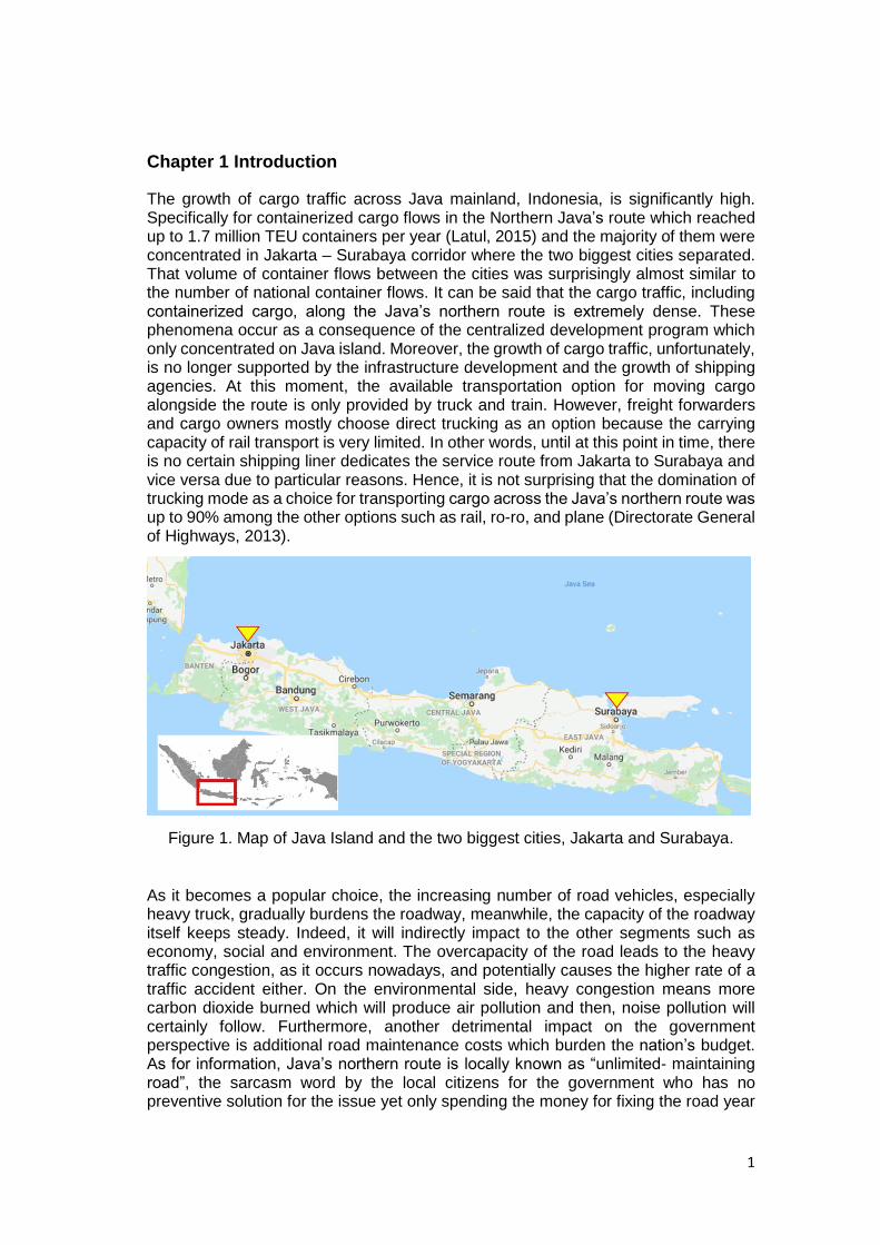
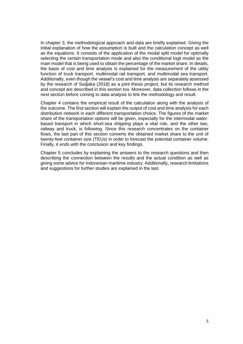
The growth of cargo traffic across Java mainland, Indonesia, is significantly high. Specifically for containerized cargo flows in the Northern Java’s route which reached up to 1.7 million TEU containers per year (Latul, 2015) and the majority of them were concentrated in Jakarta – Surabaya corridor where the two biggest cities separated. That volume of container flows between the cities was surprisingly almost similar to the number of national container flows. It can be said that the cargo traffic, including containerized cargo, along the Java’s northern route is extremely dense. These phenomena occur as a consequence of the centralized development program which only concentrated on Java island. Moreover, the growth of cargo traffic, unfortunately, is no longer supported by the infrastructure development and the growth of shipping agencies. At this moment, the available transportation option for moving cargo alongside the route is only provided by truck and train. However, freight forwarders and cargo owners mostly choose direct trucking as an option because the carrying capacity of rail transport is very limited. In other words, until at this point in time, there is no certain shipping liner dedicates the service route from Jakarta to Surabaya and vice versa due to particular reasons. Hence, it is not surprising that the domination of trucking mode as a choice for transporting cargo across the Java’s northern route was up to 90% among the other options such as rail, ro-ro, and plane (Directorate General of Highways, 2013).

Figure 1. Map of Java Island and the two biggest cities, Jakarta and Surabaya.

As it becomes a popular choice, the increasing number of road vehicles, especially heavy truck, gradually burdens the roadway, meanwhile, the capacity of the roadway itself keeps steady. Indeed, it will indirectly impact to the other segments such as economy, social and environment. The overcapacity of the road leads to the heavy traffic congestion, as it occurs nowadays, and potentially causes the higher rate of a traffic accident either. On the environmental side, heavy congestion means more carbon dioxide burned which will produce air pollution and then, noise pollution will certainly follow. Furthermore, another detrimental impact on the government perspective is additional road maintenance costs which burden the nation’s budget. As for information, Java’s northern route is locally known as “unlimited- maintaining road”, the sarcasm word by the local citizens for the government who has no preventive solution for the issue yet only spending the money for fixing the road year

2

by year, instead. Most importantly, the issues also possibly affect the logistics cost, for instances, higher fuel consumption and additional travel time as consequences of heavy congestion can be the causes of higher logistics cost. In comparison with the ASEAN countries, Indonesia remains behind its neighbors, Singapore and Malaysia, for the Logistics Performance Index (LPI) ranking (World Bank, 2017).

A preventive action should be executed to reduce the traffic jam and solve the other issues as well as provide adequate delivery services across the Java’s northern route. It is proposed a potential alternative in which employing a vessel as part of delivery cargo over the short route or commonly known as short sea shipping. Short sea shipping can be defined as the activity of transporting cargo in the short distance between the islands, between mainland, between the island and mainland or vice versa, or along the coastal line (US Maritime Administration, 2005). It might be geographically suitable for a country like Indonesia whereby as known as a maritime country with a thousand islands and thousand kilometers of coastal line. On the other side of the globe, Short sea shipping program has been successfully employing in Europe for transporting container from deep-sea terminal to the local port using feeder liner. It is also to be implemented in Vietnam for inland and coastal waterways (Blancas and Baher, 2013). By utilizing short sea shipping as part of multimodal sea transportation, it hopefully can shift the cargo which previously carried by truck to partly using a vessel as its main transportation mode. It is worth to note that transporting container by ship promises bigger carried capacity that leads to economies of scale. Thus, the fuel consumption and pollution per TEU container will relatively lower as well as reducing traffic congestion and the overload of the roadway.

1.1. Research objectives

The fundamental background of this research is the unsolved congestion problem and the other disputed issues regarding the national roadway, the Northern Java’s route or as locally known as ‘Jalur Pantura’ - Indonesia, which always becomes a long-debatable discussion topic year by year. Another reason, as a maritime country, sea carriage is indeed a potential transportation mode for Indonesia, but unfortunately, it is still not optimally developed. Nowadays, Truck and railroad are dominated as the only option for conveying goods across the northern coast, but the infrastructure seems no longer sufficient to provide all the demand. Hence, this research will propose the idea of utilizing national’s potential ability in the maritime sector to solve the problematic issues.

The research’s main objective is, therefore, giving the quantitative figure of a potential market share of the alternative transportation option, namely short sea shipping, as well as estimated container transported annually. However, short sea shea shipping is defined in this research as part of intermodal water transport which applied by connecting origin-destination place by a combination of both vessel and trucking. The principal point is obviously in the utilization of vessel part which will be applied for transporting cargo in Jakarta - Surabaya corridor. Furthermore, the feasibility of using a vessel will be expressed by the value of the potential market share and total TEUs container carried which are formed by the conditional logit model given estimated operational cost and delivery time as the attribute. Regardless, vessel cost and travel time estimation are separately assessed in “Feasibility Study of a Maritime Jalur Pantura (Java Northern Coast Line): An Economic Evaluation of a Direct Shipping Line Service Between Jakarta and Surabaya” - MEL thesis 2018 by Gregory Alfred Sudjaka as a joint thesis project. Finally, the share of multimodal seagoing transport will be compared with the existing choice (railway and road) whether it is feasible or

3

not to be applied as an alternative transportation across the northern Java’s route. To be noted, the research focuses on the containerized cargo flows between two metropolitan area of Indonesia, Jakarta and Surabaya, as well as including the cities surroundings.

1.2. Research question and sub-research questions

The main question of this research is to answer as follows:

How are the potential market share and transported container volume by the alternative transportation mode, short sea shipping, in the northern Java’s route?

The following sub-research questions must be acknowledged to adequately answer the main question above :

1. What is the estimated total cost for moving cargo using direct trucking, multimodal rail transport and multimodal short sea shipping across the northern Java’s Route?

2. What is the estimated travel time for transporting cargo along the northern Java’s route for each different transportation mode (truck, multimodal rail transport, and multimodal sea transport)?

1.3. Research design and methodology

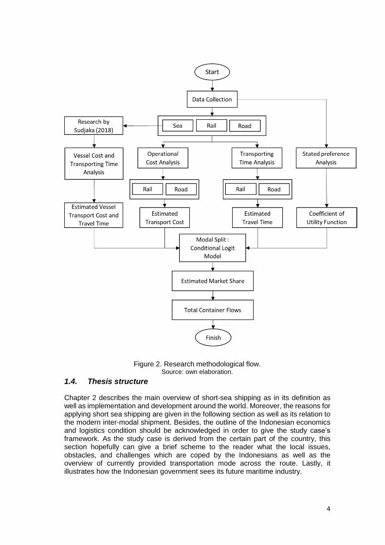
To answer the main question regarding market share and carried container volume, three types of analysis for each delivery option will be governed respectively, namely cost analysis, time analysis and stated preference analysis in order to derive the utility functions. Afterward, the calculation of the conditional logit model is conducted based on the calculated utility functions in which therefore will produce estimated market share for three different modes. Figure 2 illustrates a schematic flow of how to conduct the research.

The data collection is divided into three different concerns; cost, time and stated preference. It is worth mentioning that this research uses containerized freight as transported cargo. Operational cost and travel time, thus, generate the utility function of three different transportation choices in a single voyage. To simplify the research and due to the time constraint, operational cost and travel time are the only attributes assessed as the most considered factor for the decision makers to deliver the cargo. Besides, the estimation of cost and time by a vessel is separately done by the thesis of G. A. Sudjaka (2018) in “Feasibility Study of a Maritime Jalur Pantura (Java Northern Coast Line): An Economic Evaluation of a Direct Shipping Line Service Between Jakarta and Surabaya” as a joint thesis project.

To put it another way, stated preference analysis should be exercised to extract the coefficient of the utility function which counted as the basic choice made by the parties involved. The value of the coefficient can be gained by directing a personal interview to the main transportation actors which is, in this case, is freight forwarders. Freight forwarders more likely have their own authority to decide which transport mode should be selected, so it makes them capable as a decision maker of transportation choice according to the idea of Bergantino and Bolis (2004). At the end of the research, by the calculated market share of the three different modal choices, estimated total cargo flows, in TEUs, can be projected in each transportation mode.

4

Figure 2. Research methodological flow. Source: own elaboration.

1.4. Thesis structure

Chapter 2 describes the main overview of short-sea shipping as in its definition as well as implementation and development around the world. Moreover, the reasons for applying short sea shipping are given in the following section as well as its relation to the modern inter-modal shipment. Besides, the outline of the Indonesian economics and logistics condition should be acknowledged in order to give the study case’s framework. As the study case is derived from the certain part of the country, this section hopefully can give a brief scheme to the reader what the local issues, obstacles, and challenges which are coped by the Indonesians as well as the overview of currently provided transportation mode across the route. Lastly, it illustrates how the Indonesian government sees its future maritime industry.

5

In chapter 3, the methodological approach and data are briefly explained. Giving the initial explanation of how the assumption is built and the calculation concept as well as the equations. It consists of the application of the modal split model for optimally selecting the certain transportation mode and also the conditional logit model as the main model that is being used to obtain the percentage of the market share. In details, the basis of cost and time analysis is explained for the measurement of the utility function of truck transport, multimodal rail transport, and multimodal sea transport. Additionally, even though the vessel’s cost and time analysis are separately assessed by the research of Sudjaka (2018) as a joint thesis project, but its research method and concept are described in this section too. Moreover, data collection follows in the next section before coming to data analysis to link the methodology and result.

Chapter 4 contains the empirical result of the calculation along with the analysis of the outcome. The first section will explain the output of cost and time analysis for each distribution network in each different transportation choice. The figures of the market share of the transportation options will be given, especially for the intermodal water-based transport in which short-sea shipping plays a vital role, and the other two, railway and truck, is following. Since this research concentrates on the container flows, the last part of this section converts the obtained market share to the unit of twenty-feet container size (TEUs) in order to forecast the potential container volume. Finally, it ends with the conclusion and key findings.

Chapter 5 concludes by explaining the answers to the research questions and then describing the connection between the results and the actual condition as well as giving some advice for Indonesian maritime industry. Additionally, research limitations and suggestions for further studies are explained in the last.

6

Chapter 2 Short sea shipping and Indonesian supply chain and logistics

Literature review needs to be conducted to give the general outline of the research. This chapter provides two major literature understanding suchlike the term of short sea shipping itself and Indonesian logistics condition. The first part defines the term of short sea shipping, including how it is developed and implemented in the several areas, the fundamental background why the countries should start their short sea shipping program, and the strong connection between short sea shipping and intermodal container-based transportation. Because the research’s case takes place in the particular area of Indonesia, the second part of this chapter will principally talk about the case’s location, which is Indonesia in general, and Java island in specific. It starts from the explanation of national logistics network situation, the issues occurred in northern Java’s route, the current condition of provided transportation choices along the north coast route, and finally comes to the maritime-related government plans.

2.1. Short sea shipping as an alternative transportation

2.1.1. Definition of short sea shipping

As technology developed, the system of transportation evolves to the modern stage. It is supported by Stopford’s statement (2009) that the conventional transportation system is now gradually modified to the modern one, especially for the international freight transport, it consists of railways, roads, inland waterways, air freight services and shipping lines. He illustrated three zones laid in the new transport system:

- Inter-regional transport; Transporting cargo by deep-sea vessel or air freight between the countries or continents.

- Short-sea shipping; Transporting cargo in short distance and regularly providing a service for deep-sea vessel’s cargo to be distributed along the surrounding regions.

- Inland transport; Transporting cargo over the mainland using the road, rail, barge and canal transport.

Short sea shipping offers a service to deliver goods within regions, give an example, after container has been discharged in Port of Rotterdam, as a regional point, by the deep-sea vessel, it is then shipped by a smaller vessel varying in size from 400 DWT to 6000 DWT in port-to-port service to the neighbouring areas such as Dusseldorf, Frankfurt, or within the Netherlands regions. Regarding inland transport, several transportation options are sometimes provided, such as land-based carriage of truck or rail, therefore, direct competition typically occurred among the modes (Stopford, 1997).

Theoretically, the definition of short sea shipping is cannot easily specify by the experts since they have own explanation based on the implementation in each region. Hence, The absence of the universal definition of short sea shipping has directed to methodological issues and complications for making policy, analyzing market, conceptualizing strategy, and conducting research around the 1990s. As a consequence, the multiple perceptions became a preventive concern to develop public policy initiatives and examine the market situations which are crucial for business objectives (Lombardo, 2004). Moreover, the differentiation of the definition used, the flow of consideration most likely might adjust as well (Peeters, 1993; Blonk,

7

1993b). Balduni provided the first academic definition of short sea shipping in 1982, short sea shipping is known as water transportation between seaports of a country and between a local’s port and the ports of neighboring nations (Balduni, 1982). Service type, as well as the introduction of cabotage and the various aspects, is included in the initial interpretation as stated by the European Commission ten years later, it is transporting passenger and cargo by sea between seaports placed among the ports of member state to the other states or between non-EU ports having a shoreline on the surrounded seas bordering Europe (Commission of the European Communities, 1992). Meanwhile, Bjornland argued short sea shipping is not involving an ocean in its sailing activities (Bjornland, 1993), that was in line with the definition stated by the US Maritime Administration (US Department of Transportation, 2008). The maximum vessel size limited to 5000 gross tonnages in the early interpretation of short sea shipping by a subjective consideration (Criley and Dean, 1993). But it was debated by Bagchus and Kuipers who said limiting the size of vessel used in short sea shipping service is not relatable, the size of the vessel can be free to decide whether it is small, large, or coastal type (Bagchus and Kuipers, 1993), as well as the number of ships deployed, is in the authority of shipping company itself (Paixao and Marlow, 2002). As it was introduced in the early years, Short sea shipping organization had coordination and cooperation issues among the transportation actors, such as truck operators (Van Gunsteren et al., 1993). This was because of the lack of industrial innovation, and inadequacy persuading and marketing movements through the short sea shipping industry (Van Willigenburg and Hollander, 1993). Greek experts segmented the market of short sea shipping in two different variety; ferries and freight, including bulk and general cargo (Psaraftis and Papanikolaou, 1993). In contrary idea, the markets relatively can be separated into four categories according to Hoogerbeets and Melissen; traditional single-deck bulk vessel, container feeder ship, ferries, bulk and tankers (Hoogerbeets and Melissen, 1993).

2.1.2. Development and Implementation of short sea shipping

Short sea shipping is not a new concept in the worldwide maritime transport. In the last decades, policies regarding implementation of short sea shipping have been employed in some countries in order to promote this alternate transport. European countries have been implemented short sea shipping quite well, even though it has not yet fully fledged. The European technology advances bring the short sea shipping program into the highest level such as the efficiency of cargo handling and optimal vessel speed. The evolution of European short sea shipping starts from a deep-sea vessel provider service to an integrated door-to-door multimodal function among European cities. Moreover, the short sea shipping industry has been attracting deep-sea vessel operators to invest their business in the coastal liner (Brooks and Frost, 2004). At the beginning of 1990, research and subsidy programs were conducted by the European Commission in order to promote short sea shipping. Initiated by the Concerted Action on Short Sea Shipping, approximately 44 studies published by 1996 (Psaraftis and Schinas, 1996). Total 13 states, including Norway, are participated in promoting short sea shipping program under the European Shortsea Network, namely Short Sea Shipping Promotion Centres (COM, 2003). In 1992, The Pilot Action for Combined Transport (PACT) program was introduced, it already invested total 53 million Euro for 167 projects within 8 years from 1992 to 2000 (European Comission, 2001). The PACT was then replaced by the Marco Polo I and II programmes and

8

responsible as a financial provider to potential short sea shipping services which have spent up to 750 million Euro regarding the re-establishment of the coastal liner. The primary objective is shifting at least 30 percent of cargo carried by road to the other alternate options such as railway and short sea shipping by 2030 and further increase by 20% more in 2050 (COM, 2011).

In the United States, The US Maritime Administration (MarAd) take a role to encourage short sea shipping to be the alternative transport option. This action was taken since the government couldn’t control the growing freight congestion on US’s railway and highway system. Thus, the utilization of maritime-based transport needs to be promoted with the aim to reduce air pollution and ease traffic jam (Brooks and Frost, 2004). The program has been highly prioritized by the US Department of Transportation since 2002. With identical concept with EU, the US short sea shipping system is developed to connect the offshore island regions, containing Hawaii, Alaska, and Puerto Rico, to the nation’s mainland as well as escalating intermodal capability by way of the underutilized waterways along the national coastal line (Perakis and Denisis, 2008). In order to integrate short sea shipping network, Memorandum of Cooperation on Sharing Short Sea Shipping Information and Experience between the United States and the neighboring countries, such as Canada and Mexico, was signed on 16 July 2013. Moving to the US’s neighbor country, Canada, the short sea shipping movement is slightly dynamic on the east coast of the country because it combines modern and old technology regarding utilization of the vessel. The issues faced by the local authority nowadays are the expensive cost of new vessel construction in the local shipyards and the 25% tax on operating foreign-built vessels across Canadian coastal lines (Brooks and Frost, 2004).

Short sea shipping is also commonly applied in South East Asia countries since the majority of the countries geographically is an island country. Vietnam introduced the program of coastal shipping and Inland Waterway Transport (IWT) to utilize two enormous river deltas and 3000 kilometers of coastline. Therefore, Short sea shipping is crucial for Vietnamese on the daily basis for supporting their economic activity and development (Blancas and Baher, 2013). Sometimes, short sea shipping is controlled by numerous political constraints such as cabotage. For instance in Indonesia, the country implements short sea shipping as its main carriage to trade the goods among the islands. Nevertheless, only Indonesian-flag vessel can sail and transport cargos among the islands which included in Indonesian territory. The foreign-flag deep-sea vessel can only drop the goods in the certain port of Indonesia such as main port Jakarta or Surabaya, and then, short sea shipping is implemented as a distributor of deep-sea vessel’s cargo to the other domestic destinations. Moreover, cabotage is regularly employed in the country that has a very long coastal line, another case is the United States and Brazil. Sánchez and Wilmsmeier (2005) and Bendall and Brooks (2011) are also giving some examples of short sea shipping application in Oceania and Latin America. Meanwhile, in North East Asia, short sea shipping is a powerful concept, it is strongly connected between South Korea, Japan and China (Medda and Trujillo, 2014). Taking everything into account, the potential for short sea shipping has been successfully developed and implemented worldwide.

2.1.3. Fundamental reasons for conducting short sea shipping

Every country has its own reasons and objectives for employing short sea shipping as an alternative transport in order to solve its national problems. The reason of economics, social, or environment commonly become a basic background of the

9

decision to obtain an alternative of transportation mode. However, many governments are in the same vision with economics study that believes short sea shipping is the best transportation choice on the environmental point of view (Suárez-Alemán et al, 2014).

In the EU, the transportation industry has become the quickest growing energy consumer since 1985 with 47% rate (Eurostat, 2006). Besides, Medda and Trujillo (2014) found that road transport, above all, experienced the most-increased volume of goods transported in tonnes-km. They added, externalities caused by transport industry, in general, associates to the time, geographical location, weather, transport category, and users. It is worth to take into account that transportation’s external costs represent 8% of the Gross Domestic Product (GDP) (Whitelegg, 1977). Moreover, uncontrolled consumption of fossil-based fuel for transportation activity becomes the main issue in developing countries. Thus, the role of short sea shipping, either as part of multimodal transport network or unimodal alternate option, is assessed as a feasible alternative to reduce external cost such as uncontrollable consumption of energy and gas emission induced by freight transport (Realise, 2002).

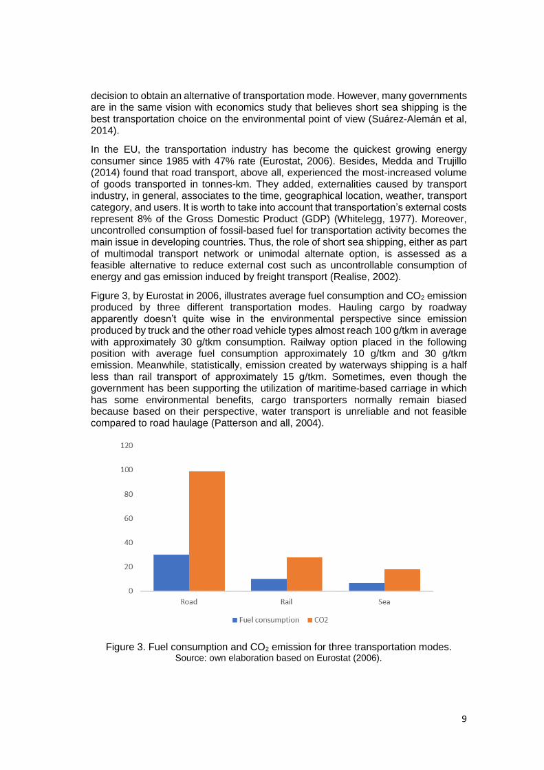
Figure 3, by Eurostat in 2006, illustrates average fuel consumption and CO2 emission produced by three different transportation modes. Hauling cargo by roadway apparently doesn’t quite wise in the environmental perspective since emission produced by truck and the other road vehicle types almost reach 100 g/tkm in average with approximately 30 g/tkm consumption. Railway option placed in the following position with average fuel consumption approximately 10 g/tkm and 30 g/tkm emission. Meanwhile, statistically, emission created by waterways shipping is a half less than rail transport of approximately 15 g/tkm. Sometimes, even though the government has been supporting the utilization of maritime-based carriage in which has some environmental benefits, cargo transporters normally remain biased because based on their perspective, water transport is unreliable and not feasible compared to road haulage (Patterson and all, 2004).

Figure 3. Fuel consumption and CO2 emission for three transportation modes. Source: own elaboration based on Eurostat (2006).

10

According to the study by Medda and Trujillo (2014), Externality costs are divided into two categories; harm cost and prevention cost. The external damages occurred due to transport activities is counted as the cost of harm. Whilst, the cost of prevention measures the action cost for preventing the damage from occurring. Therefore, four main external cost can be identified according to those paired categories:

- Air pollution; environmental quality degradation caused by chemical particles such as SO2 and NO2. The cost estimation for air pollution is complicated to measure since there is no market value on it and remains under discussion, a lot of factors determine air pollution but it can be identified based on the specific location (SCOOP, 2004) (UNITE, 2002) (UNITE, 2003).

- Infrastructure cost; issues occurred because of transport activities along the certain infrastructures such as overload capacity of roadways that caused preliminary road maintenances.

- Noise emission; measured by the noise level produced by cargo trucks on the highway. Noise pollution by trucks dominate approximately two-thirds of shares in the United States highway (GAO, 2005)

- Congestion cost; the delay cost caused when the roadways experience overcapacity of traffic. Contributes more than 50% of total cost (Henesey and Yonge, 2006).

Several studies related to the external cost caused by transport modes have been conducted and all concluded that the utilization of short sea shipping as part of intermodal freight transport impacts less to the external cost than the other which is not included water-based transport. A research which observed certain European corridor, from Genoa - Italy to Preston - UK, deduced that the goods transported involving short sea shipping reduces half of the external cost compared to only using road transport (Ricci and Black, 2005). Another study conducted in the US routes, New York to Miami and New York to Boston, also proves similar comparative benefits of short sea shipping utilizations (Henesey and Yonge, 2006). Once the comparison of intermodal sea transport cost and direct trucking cost is relatively small, then involvement of both public and financial advantages of short sea shipping contributes 35–45% reduction of total transport costs (SCOOP, 2004).

Apart from environmental aspects, carried capacity plays another role to benefit water freight mode. Employing the concept of economies of scale and distance, shipping operators promise a lower freight rate in comparison with other options. Despite the fact that a capital-intensive industry of shipping in general, and short ship shipping in specific, which could be seen as a weak point because the unstable market nature and considered as high barrier for business entrance, the truth is that this point is also can be observed as a potency due to it proves that the shipping actors already have their own power to develop the transport systems (Paixao and Marlow, 2002). On the other perspective, sea-based carriage requires the lowest cost of supporting infrastructure. Moving commodities via sea doesn’t need construction cost to build the sea-way and it provides the essentially infinite capacity. The only cost it needs only port investment and maintenance, in comparison with road and rail, they need higher external cost which always increases significantly. Road and railway networks oblige huge investment in order to develop the infrastructures such as road and railways, bridges, and tunnels. Meanwhile, to operate a vessel, port area is the only land space needed. According to the utilization of land space, it can be concluded that short sea shipping is environmentally friendly (Paixao and Marlow, 2004).

11

2.1.4. Intermodal container transport

As a consequence of time, cost, and space limitation and optimization, it brings the idea for the utilization of multiple transportation modes in order to move the passengers or goods. Transporting passenger or goods from origin to destination place using two or more transportation modes is basically described as multimodal or Intermodal shipment. Meanwhile, the Intermodal terminal is commonly known as the transit place between the modal shifts.

In accordance with the universality of cargo handling, container-based cargo is counted as the easiest goods to handle and move. Therefore, the application of intermodal freight transport in the container industry is working well as of today. A container unit efficiently works in the majority of all transportation modes such as truck, rail, barge, or vessel. Hence, mostly the intermodal container carriage consists at least by two of them. As stated above, freight forwarders or shippers regularly decide to use multiple modals due to the objective of cost and time optimization or in case of spacial restrictions when using unimodal freight transport. Consequently, transport operators who join the multimodal market experience a tight competition among the transportation modes. For instances, truck competes with rail, short sea shipping with road and rail, and air transport with deep-sea shipping (Stopford, 2009). Moreover, Suarez-Aleman and all (2014) hypothetically stated that the transporting time of intermodal freight transport which including short sea shipping counts as a primary issue. Compared to the deep-sea shipping, delivery time competition among the other modes is not an issue due to its carriage type or geographical condition (Suarez-Aleman and all, 2014).

However, containerized intermodal transportation is predicted constantly rising in the upcoming years along with the development of the economic, technological environment, and regulation of the industry (Crainic and Kap, 2007). Thus, it is a big opportunity, then all the facilities, technologies, or organization managements need to be prepared in order to bring the new transportation era to be more sustainable and environmentally friendly.

2.2. Overview of short sea shipping, supply chain, and logistics flows in Indonesia

2.2.1. Indonesian logistics networks

Connecting islands in order to meet integrated logistics system are such a disputable issue for archipelago countries. Consequently, the economics developments sometimes tend to be centralized in the particular areas and impacting to the massive economic gap among the islands, regions or cities. Indonesian people these days cope with the identical issue regarding equalization of domestic logistics distribution. However, problematic infrastructure and facility supports are reasonably accused to be the primary issue of insufficient supply chain and logistics networks. Stated of Logistics Indonesia (2015) claimed that the domestic logistics cost touched 24.66% proportion of national Gross Domestic Product (GDP).

12

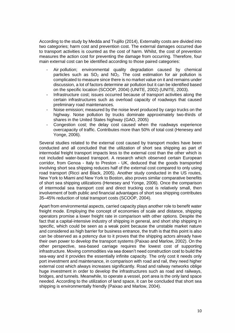
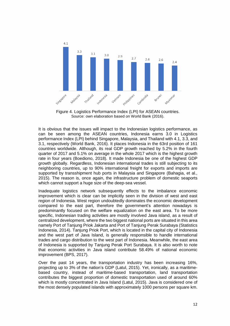
Figure 4. Logistics Performance Index (LPI) for ASEAN countries. Source: own elaboration based on World Bank (2016).

It is obvious that the issues will impact to the Indonesian logistics performance, as can be seen among the ASEAN countries, Indonesia earns 3.0 in Logistics performance Index (LPI) behind Singapore, Malaysia, and Thailand with 4.1, 3.3, and 3.1, respectively (World Bank, 2016). It places Indonesia in the 63rd position of 161 countries worldwide. Although, its real GDP growth reached by 5.2% in the fourth quarter of 2017 and 5.1% on average in the whole 2017 which is the highest growth rate in four years (Boediono, 2018). It made Indonesia be one of the highest GDP growth globally. Regardless, Indonesian international trades is still subjecting to its neighboring countries, up to 90% international freight for exports and imports are supported by transshipment hub ports in Malaysia and Singapore (Bahagia, et al., 2015). The reason is, once again, the infrastructure problem of domestic seaports which cannot support a huge size of the deep-sea vessel.

Inadequate logistics network subsequently effects to the imbalance economic improvement which is clear can be implicitly seen in the division of west and east region of Indonesia. West region undoubtedly dominates the economic development compared to the east part, therefore the government’s attention nowadays is predominantly focused on the welfare equalization on the east area. To be more specific, Indonesian trading activities are mostly involved Java island, as a result of centralized development, where the two biggest national ports are situated in this area namely Port of Tanjung Priok Jakarta and Port of Tanjung Perak Surabaya (Statistics Indonesia, 2014). Tanjung Priok Port, which is located in the capital city of Indonesia and the west part of Java Island, is generally responsible to handle international trades and cargo distribution to the west part of Indonesia. Meanwhile, the east area of Indonesia is supported by Tanjung Perak Port Surabaya. It is also worth to note that economic activities in Java island contribute 58.49% of national economic improvement (BPS, 2017).

Over the past 14 years, the transportation industry has been increasing 16%, projecting up to 3% of the nation’s GDP (Latul, 2015). Yet, ironically, as a maritime-based country, instead of maritime-based transportation, land transportation contributes the biggest proportion of domestic transportation used of around 60% which is mostly concentrated in Java Island (Latul, 2015). Java is considered one of the most densely populated islands with approximately 1000 persons per square km.

13

According to the statement of Indonesian Ministry of Industry, approximately 75% Industrial regency is centralized on Java island, and the other 25% is scattered outside Java. It can be imagined how busy the cargo traffic for in-and-out and within the island is. Moreover, the utilization of land haulage for moving commodities over the island is significantly dominating up to 99% of the market (Supply Chain Indonesia, 2016b). Thus, that fact obviously causes to the various problems such as traffic congestions, insufficient infrastructures, pollutions or even social issues.

2.2.2. The Northern Java’s route

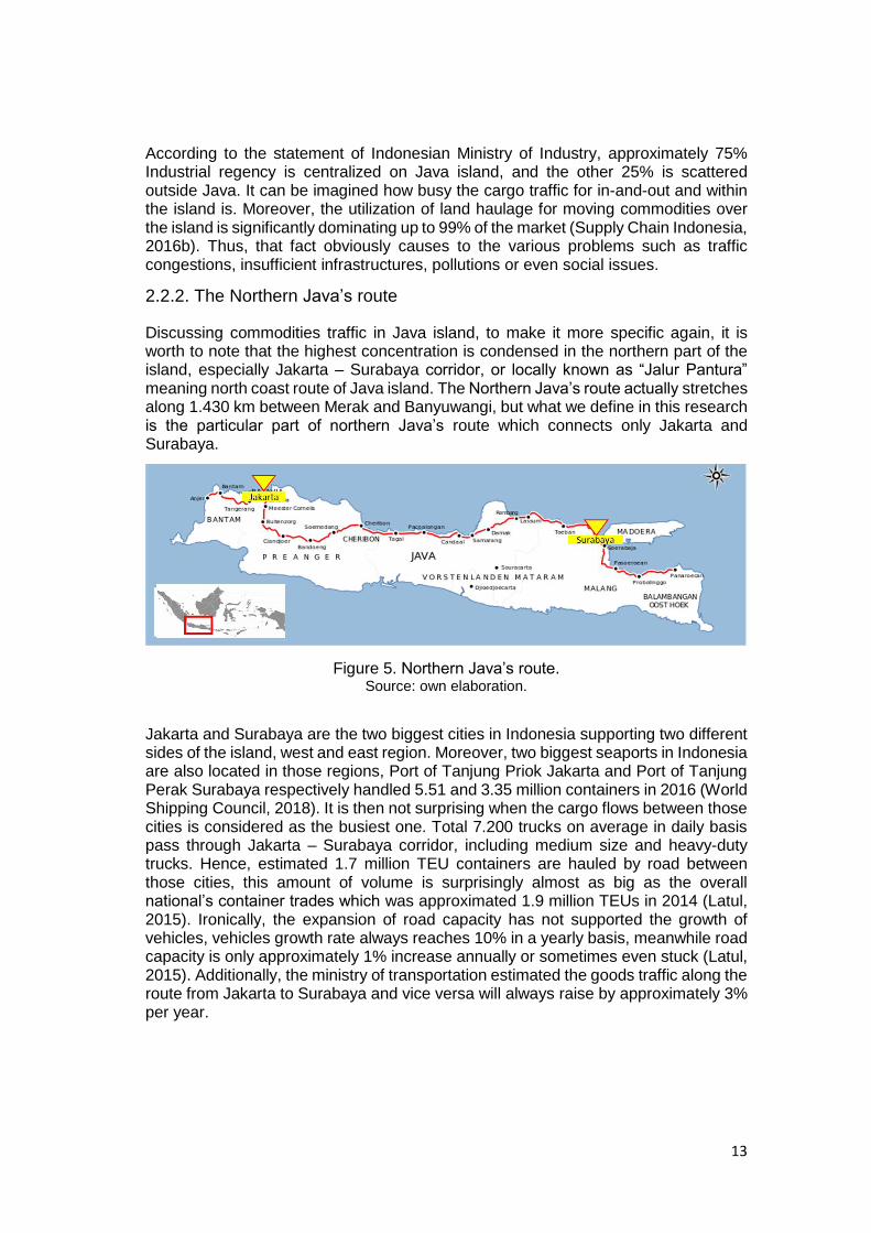
Discussing commodities traffic in Java island, to make it more specific again, it is worth to note that the highest concentration is condensed in the northern part of the island, especially Jakarta – Surabaya corridor, or locally known as “Jalur Pantura” meaning north coast route of Java island. The Northern Java’s route actually stretches along 1.430 km between Merak and Banyuwangi, but what we define in this research is the particular part of northern Java’s route which connects only Jakarta and Surabaya.

Figure 5. Northern Java’s route. Source: own elaboration.

Jakarta and Surabaya are the two biggest cities in Indonesia supporting two different sides of the island, west and east region. Moreover, two biggest seaports in Indonesia are also located in those regions, Port of Tanjung Priok Jakarta and Port of Tanjung Perak Surabaya respectively handled 5.51 and 3.35 million containers in 2016 (World Shipping Council, 2018). It is then not surprising when the cargo flows between those cities is considered as the busiest one. Total 7.200 trucks on average in daily basis pass through Jakarta – Surabaya corridor, including medium size and heavy-duty trucks. Hence, estimated 1.7 million TEU containers are hauled by road between those cities, this amount of volume is surprisingly almost as big as the overall national’s container trades which was approximated 1.9 million TEUs in 2014 (Latul, 2015). Ironically, the expansion of road capacity has not supported the growth of vehicles, vehicles growth rate always reaches 10% in a yearly basis, meanwhile road capacity is only approximately 1% increase annually or sometimes even stuck (Latul, 2015). Additionally, the ministry of transportation estimated the goods traffic along the route from Jakarta to Surabaya and vice versa will always raise by approximately 3% per year.

14

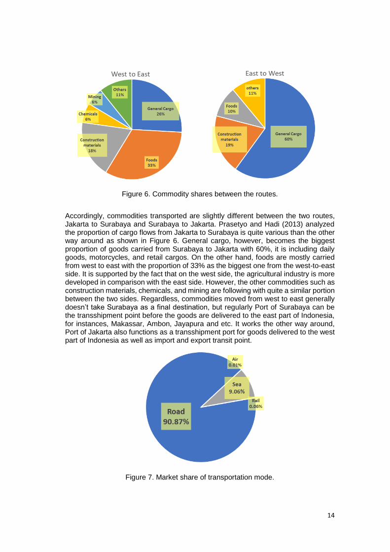
Figure 6. Commodity shares between the routes.

Accordingly, commodities transported are slightly different between the two routes, Jakarta to Surabaya and Surabaya to Jakarta. Prasetyo and Hadi (2013) analyzed the proportion of cargo flows from Jakarta to Surabaya is quite various than the other way around as shown in Figure 6. General cargo, however, becomes the biggest proportion of goods carried from Surabaya to Jakarta with 60%, it is including daily goods, motorcycles, and retail cargos. On the other hand, foods are mostly carried from west to east with the proportion of 33% as the biggest one from the west-to-east side. It is supported by the fact that on the west side, the agricultural industry is more developed in comparison with the east side. However, the other commodities such as construction materials, chemicals, and mining are following with quite a similar portion between the two sides. Regardless, commodities moved from west to east generally doesn’t take Surabaya as a final destination, but regularly Port of Surabaya can be the transshipment point before the goods are delivered to the east part of Indonesia, for instances, Makassar, Ambon, Jayapura and etc. It works the other way around, Port of Jakarta also functions as a transshipment port for goods delivered to the west part of Indonesia as well as import and export transit point.

Figure 7. Market share of transportation mode.

15

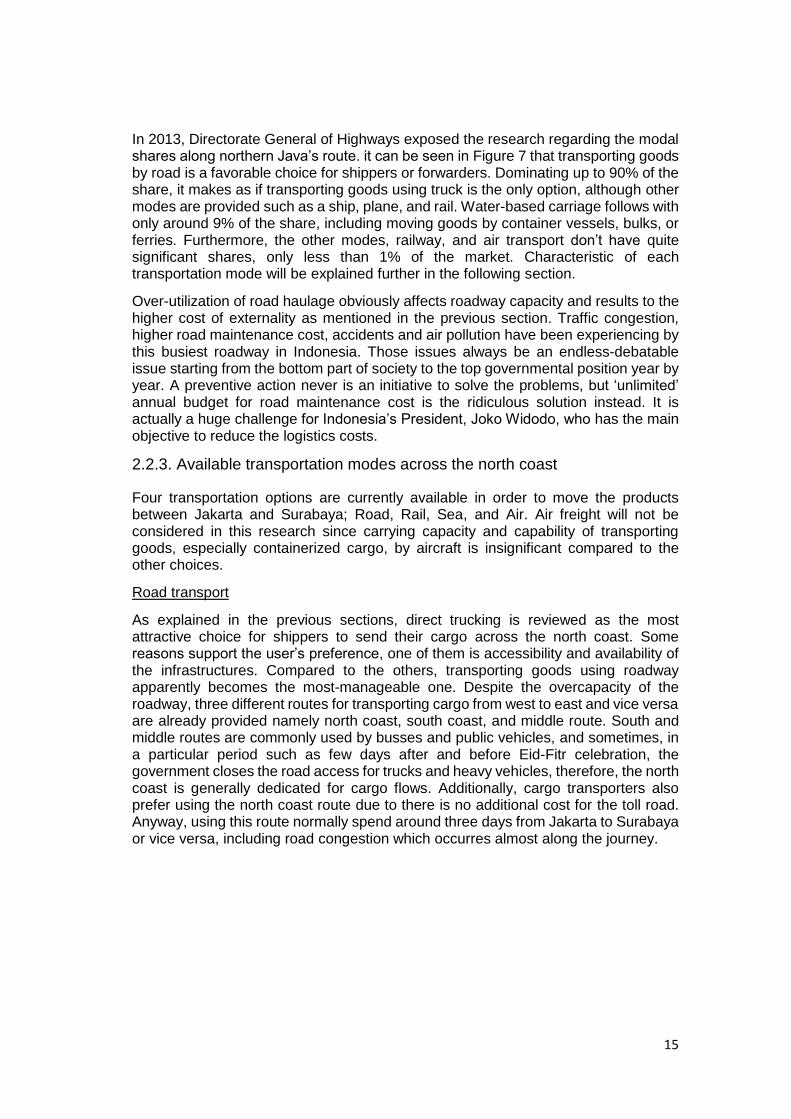
In 2013, Directorate General of Highways exposed the research regarding the modal shares along northern Java’s route. it can be seen in Figure 7 that transporting goods by road is a favorable choice for shippers or forwarders. Dominating up to 90% of the share, it makes as if transporting goods using truck is the only option, although other modes are provided such as a ship, plane, and rail. Water-based carriage follows with only around 9% of the share, including moving goods by container vessels, bulks, or ferries. Furthermore, the other modes, railway, and air transport don’t have quite significant shares, only less than 1% of the market. Characteristic of each transportation mode will be explained further in the following section.

Over-utilization of road haulage obviously affects roadway capacity and results to the higher cost of externality as mentioned in the previous section. Traffic congestion, higher road maintenance cost, accidents and air pollution have been experiencing by this busiest roadway in Indonesia. Those issues always be an endless-debatable issue starting from the bottom part of society to the top governmental position year by year. A preventive action never is an initiative to solve the problems, but ‘unlimited’ annual budget for road maintenance cost is the ridiculous solution instead. It is actually a huge challenge for Indonesia’s President, Joko Widodo, who has the main objective to reduce the logistics costs.

2.2.3. Available transportation modes across the north coast

Four transportation options are currently available in order to move the products between Jakarta and Surabaya; Road, Rail, Sea, and Air. Air freight will not be considered in this research since carrying capacity and capability of transporting goods, especially containerized cargo, by aircraft is insignificant compared to the other choices.

Road transport

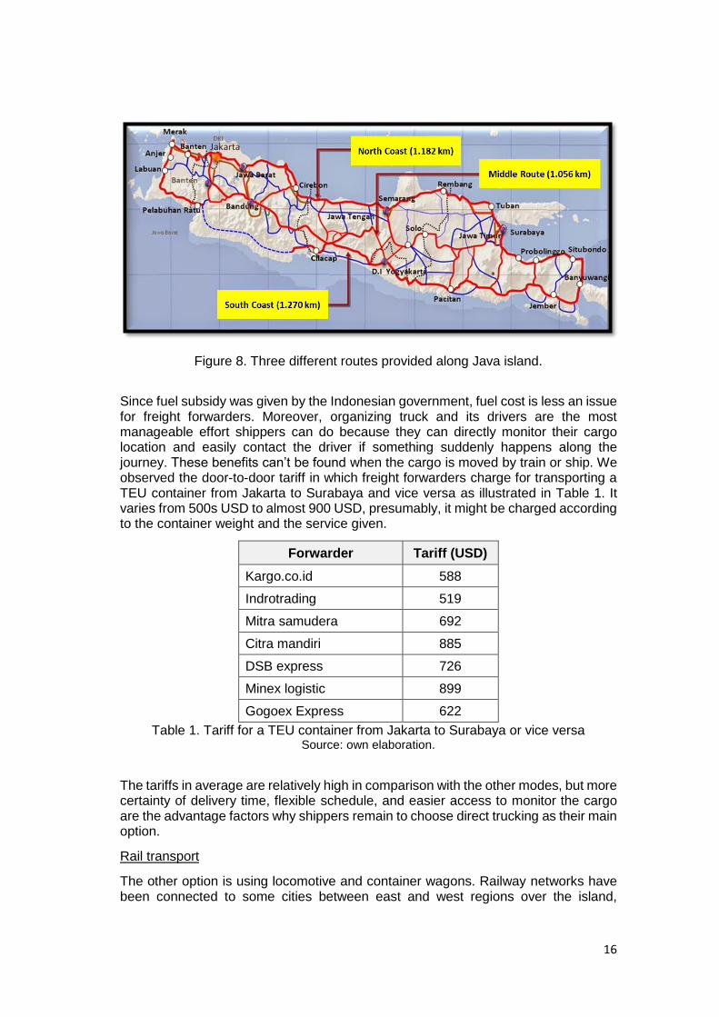
As explained in the previous sections, direct trucking is reviewed as the most attractive choice for shippers to send their cargo across the north coast. Some reasons support the user’s preference, one of them is accessibility and availability of the infrastructures. Compared to the others, transporting goods using roadway apparently becomes the most-manageable one. Despite the overcapacity of the roadway, three different routes for transporting cargo from west to east and vice versa are already provided namely north coast, south coast, and middle route. South and middle routes are commonly used by busses and public vehicles, and sometimes, in a particular period such as few days after and before Eid-Fitr celebration, the government closes the road access for trucks and heavy vehicles, therefore, the north coast is generally dedicated for cargo flows. Additionally, cargo transporters also prefer using the north coast route due to there is no additional cost for the toll road. Anyway, using this route normally spend around three days from Jakarta to Surabaya or vice versa, including road congestion which occurres almost along the journey.

16

Figure 8. Three different routes provided along Java island.

Since fuel subsidy was given by the Indonesian government, fuel cost is less an issue for freight forwarders. Moreover, organizing truck and its drivers are the most manageable effort shippers can do because they can directly monitor their cargo location and easily contact the driver if something suddenly happens along the journey. These benefits can’t be found when the cargo is moved by train or ship. We observed the door-to-door tariff in which freight forwarders charge for transporting a TEU container from Jakarta to Surabaya and vice versa as illustrated in Table 1. It varies from 500s USD to almost 900 USD, presumably, it might be charged according to the container weight and the service given.

Forwarder Tariff (USD)

Kargo.co.id 588

Indrotrading 519

Mitra samudera 692

Citra mandiri 885

DSB express 726

Minex logistic 899

Gogoex Express 622

Table 1. Tariff for a TEU container from Jakarta to Surabaya or vice versa Source: own elaboration.

The tariffs in average are relatively high in comparison with the other modes, but more certainty of delivery time, flexible schedule, and easier access to monitor the cargo are the advantage factors why shippers remain to choose direct trucking as their main option.

Rail transport

The other option is using locomotive and container wagons. Railway networks have been connected to some cities between east and west regions over the island,

17

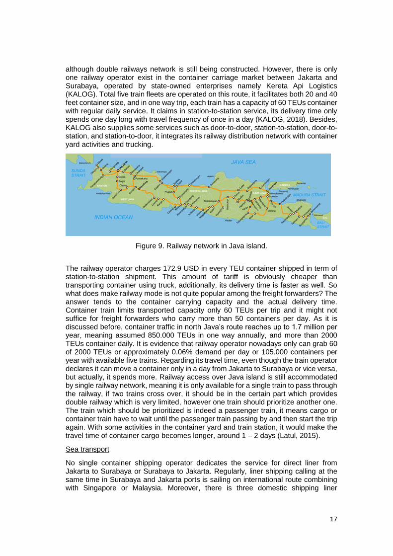
although double railways network is still being constructed. However, there is only one railway operator exist in the container carriage market between Jakarta and Surabaya, operated by state-owned enterprises namely Kereta Api Logistics (KALOG). Total five train fleets are operated on this route, it facilitates both 20 and 40 feet container size, and in one way trip, each train has a capacity of 60 TEUs container with regular daily service. It claims in station-to-station service, its delivery time only spends one day long with travel frequency of once in a day (KALOG, 2018). Besides, KALOG also supplies some services such as door-to-door, station-to-station, door-to-station, and station-to-door, it integrates its railway distribution network with container yard activities and trucking.

Figure 9. Railway network in Java island.

The railway operator charges 172.9 USD in every TEU container shipped in term of station-to-station shipment. This amount of tariff is obviously cheaper than transporting container using truck, additionally, its delivery time is faster as well. So what does make railway mode is not quite popular among the freight forwarders? The answer tends to the container carrying capacity and the actual delivery time. Container train limits transported capacity only 60 TEUs per trip and it might not suffice for freight forwarders who carry more than 50 containers per day. As it is discussed before, container traffic in north Java’s route reaches up to 1.7 million per year, meaning assumed 850.000 TEUs in one way annually, and more than 2000 TEUs container daily. It is evidence that railway operator nowadays only can grab 60 of 2000 TEUs or approximately 0.06% demand per day or 105.000 containers per year with available five trains. Regarding its travel time, even though the train operator declares it can move a container only in a day from Jakarta to Surabaya or vice versa, but actually, it spends more. Railway access over Java island is still accommodated by single railway network, meaning it is only available for a single train to pass through the railway, if two trains cross over, it should be in the certain part which provides double railway which is very limited, however one train should prioritize another one. The train which should be prioritized is indeed a passenger train, it means cargo or container train have to wait until the passenger train passing by and then start the trip again. With some activities in the container yard and train station, it would make the travel time of container cargo becomes longer, around 1 – 2 days (Latul, 2015).

Sea transport

No single container shipping operator dedicates the service for direct liner from Jakarta to Surabaya or Surabaya to Jakarta. Regularly, liner shipping calling at the same time in Surabaya and Jakarta ports is sailing on international route combining with Singapore or Malaysia. Moreover, there is three domestic shipping liner

18

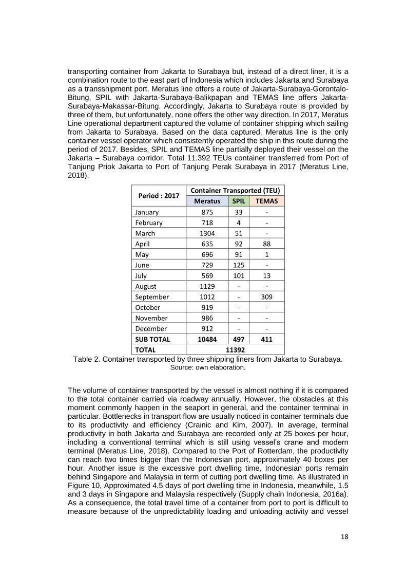
transporting container from Jakarta to Surabaya but, instead of a direct liner, it is a combination route to the east part of Indonesia which includes Jakarta and Surabaya as a transshipment port. Meratus line offers a route of Jakarta-Surabaya-Gorontalo-Bitung, SPIL with Jakarta-Surabaya-Balikpapan and TEMAS line offers Jakarta-Surabaya-Makassar-Bitung. Accordingly, Jakarta to Surabaya route is provided by three of them, but unfortunately, none offers the other way direction. In 2017, Meratus Line operational department captured the volume of container shipping which sailing from Jakarta to Surabaya. Based on the data captured, Meratus line is the only container vessel operator which consistently operated the ship in this route during the period of 2017. Besides, SPIL and TEMAS line partially deployed their vessel on the Jakarta – Surabaya corridor. Total 11.392 TEUs container transferred from Port of Tanjung Priok Jakarta to Port of Tanjung Perak Surabaya in 2017 (Meratus Line, 2018).

Period : 2017 Container Transported (TEU)

Meratus SPIL TEMAS

January 875 33 -

February 718 4 -

March 1304 51 -

April 635 92 88

May 696 91 1

June 729 125 -

July 569 101 13

August 1129 - -

September 1012 - 309

October 919 - -

November 986 - -

December 912 - -

SUB TOTAL 10484 497 411

TOTAL 11392 Table 2. Container transported by three shipping liners from Jakarta to Surabaya.

Source: own elaboration.

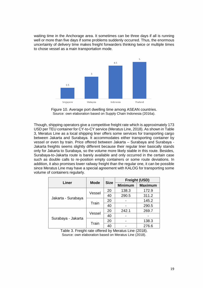
The volume of container transported by the vessel is almost nothing if it is compared to the total container carried via roadway annually. However, the obstacles at this moment commonly happen in the seaport in general, and the container terminal in particular. Bottlenecks in transport flow are usually noticed in container terminals due to its productivity and efficiency (Crainic and Kim, 2007). In average, terminal productivity in both Jakarta and Surabaya are recorded only at 25 boxes per hour, including a conventional terminal which is still using vessel’s crane and modern terminal (Meratus Line, 2018). Compared to the Port of Rotterdam, the productivity can reach two times bigger than the Indonesian port, approximately 40 boxes per hour. Another issue is the excessive port dwelling time, Indonesian ports remain behind Singapore and Malaysia in term of cutting port dwelling time. As illustrated in Figure 10, Approximated 4.5 days of port dwelling time in Indonesia, meanwhile, 1.5 and 3 days in Singapore and Malaysia respectively (Supply chain Indonesia, 2016a). As a consequence, the total travel time of a container from port to port is difficult to measure because of the unpredictability loading and unloading activity and vessel

19

waiting time in the Anchorage area. It sometimes can be three days if all is running well or more than five days if some problems suddenly occurred. Thus, the enormous uncertainty of delivery time makes freight forwarders thinking twice or multiple times to chose vessel as a main transportation mode.

Figure 10. Average port dwelling time among ASEAN countries. Source: own elaboration based on Supply Chain Indonesia (2016a).

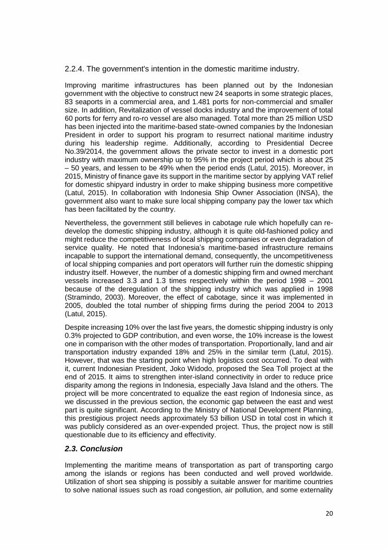
Though, shipping operators give a competitive freight rate which is approximately 173 USD per TEU container for CY-to-CY service (Meratus Line, 2018). As shown in Table 3, Meratus Line as a local shipping liner offers some services for transporting cargo between Jakarta and Surabaya. It accommodates either transporting container by vessel or even by train. Price offered between Jakarta – Surabaya and Surabaya - Jakarta freights seems slightly different because their regular liner basically stands only for Jakarta to Surabaya, so the volume more likely stable in this route. Besides, Surabaya-to-Jakarta route is barely available and only occurred in the certain case such as double calls to re-position empty containers or some route deviations. In addition, it also promises lower railway freight than the regular one, it can be possible since Meratus Line may have a special agreement with KALOG for transporting some volume of containers regularly.

Liner Mode Size Freight (USD)

Minimum Maximum

Jakarta - Surabaya

Vessel 20 138.3 172.9

40 290.5 311.2

Train 20 - 145.2

40 - 290.5

Surabaya - Jakarta

Vessel 20 242.1 269.7

40 - -

Train 20 - 138.3

40 - 276.6

Table 3. Freight rate offered by Meratus Line (2018). Source: own elaboration based on Meratus Line (2018).

20

2.2.4. The government's intention in the domestic maritime industry.

Improving maritime infrastructures has been planned out by the Indonesian government with the objective to construct new 24 seaports in some strategic places, 83 seaports in a commercial area, and 1.481 ports for non-commercial and smaller size. In addition, Revitalization of vessel docks industry and the improvement of total 60 ports for ferry and ro-ro vessel are also managed. Total more than 25 million USD has been injected into the maritime-based state-owned companies by the Indonesian President in order to support his program to resurrect national maritime industry during his leadership regime. Additionally, according to Presidential Decree No.39/2014, the government allows the private sector to invest in a domestic port industry with maximum ownership up to 95% in the project period which is about 25 – 50 years, and lessen to be 49% when the period ends (Latul, 2015). Moreover, in 2015, Ministry of finance gave its support in the maritime sector by applying VAT relief for domestic shipyard industry in order to make shipping business more competitive (Latul, 2015). In collaboration with Indonesia Ship Owner Association (INSA), the government also want to make sure local shipping company pay the lower tax which has been facilitated by the country.

Nevertheless, the government still believes in cabotage rule which hopefully can re-develop the domestic shipping industry, although it is quite old-fashioned policy and might reduce the competitiveness of local shipping companies or even degradation of service quality. He noted that Indonesia’s maritime-based infrastructure remains incapable to support the international demand, consequently, the uncompetitiveness of local shipping companies and port operators will further ruin the domestic shipping industry itself. However, the number of a domestic shipping firm and owned merchant vessels increased 3.3 and 1.3 times respectively within the period 1998 – 2001 because of the deregulation of the shipping industry which was applied in 1998 (Stramindo, 2003). Moreover, the effect of cabotage, since it was implemented in 2005, doubled the total number of shipping firms during the period 2004 to 2013 (Latul, 2015).

Despite increasing 10% over the last five years, the domestic shipping industry is only 0.3% projected to GDP contribution, and even worse, the 10% increase is the lowest one in comparison with the other modes of transportation. Proportionally, land and air transportation industry expanded 18% and 25% in the similar term (Latul, 2015). However, that was the starting point when high logistics cost occurred. To deal with it, current Indonesian President, Joko Widodo, proposed the Sea Toll project at the end of 2015. It aims to strengthen inter-island connectivity in order to reduce price disparity among the regions in Indonesia, especially Java Island and the others. The project will be more concentrated to equalize the east region of Indonesia since, as we discussed in the previous section, the economic gap between the east and west part is quite significant. According to the Ministry of National Development Planning, this prestigious project needs approximately 53 billion USD in total cost in which it was publicly considered as an over-expended project. Thus, the project now is still questionable due to its efficiency and effectivity.

2.3. Conclusion

Implementing the maritime means of transportation as part of transporting cargo among the islands or regions has been conducted and well proved worldwide. Utilization of short sea shipping is possibly a suitable answer for maritime countries to solve national issues such as road congestion, air pollution, and some externality

21

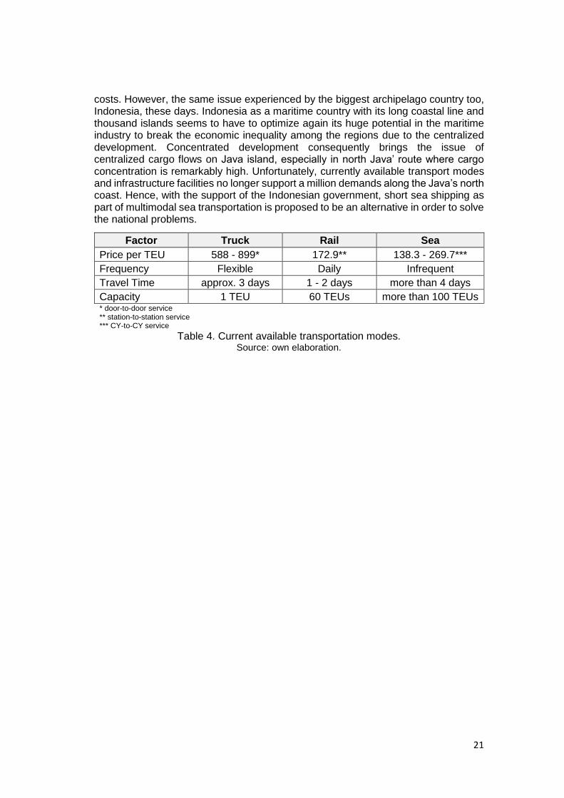
costs. However, the same issue experienced by the biggest archipelago country too, Indonesia, these days. Indonesia as a maritime country with its long coastal line and thousand islands seems to have to optimize again its huge potential in the maritime industry to break the economic inequality among the regions due to the centralized development. Concentrated development consequently brings the issue of centralized cargo flows on Java island, especially in north Java’ route where cargo concentration is remarkably high. Unfortunately, currently available transport modes and infrastructure facilities no longer support a million demands along the Java’s north coast. Hence, with the support of the Indonesian government, short sea shipping as part of multimodal sea transportation is proposed to be an alternative in order to solve the national problems.

Factor Truck Rail Sea

Price per TEU 588 - 899* 172.9** 138.3 - 269.7***

Frequency Flexible Daily Infrequent

Travel Time approx. 3 days 1 - 2 days more than 4 days

Capacity 1 TEU 60 TEUs more than 100 TEUs * door-to-door service ** station-to-station service *** CY-to-CY service

Table 4. Current available transportation modes. Source: own elaboration.

22

Chapter 3 Research methodology and data

This chapter will firstly explain the methodological approach that is used in order to generate the result, including reasons and backgrounds why the certain model should be employed. Some equations and preliminary calculations will also be enclosed to explain the main calculation concept of the research. The overview of the modal split model and the conditional logit model are described in details as well as how to obtain the coefficient of the utility function. Furthermore, the explanation of the estimated operational cost and travel time analysis will help to illustrate the calculation concept for each different mode. Secondly, data sources and data mining are included in order to convince the reliability of the result. Before coming to the next chapter, the data analysis aims to link the process between the methodological concept and the estimation result.

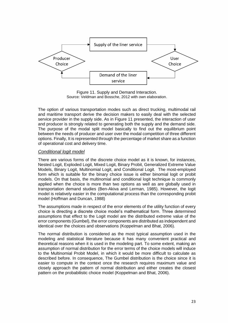
3.1. Modal split model The proposed coastal shipping service covering Jakarta-Surabaya corridor will be counted as the new alternative of the modal options over truck and rail. The service does not exist yet but we already know the demand is millions. If the scenario of the ideal condition is met, such as infrastructures and the continuous support by the government, it is not impossible that hundreds of the merchant vessel owner will compete to assist this potential service. It can be concluded that the interaction between the users (freight forwarders, cargo owners) and the producers (the shipping operators and the intermodal operators) will automatically set-up the new liner shipping service (Veldman and Bossche, 2012). Once the technical issues have been solved, the liner shipping operators then will adjust their service to meet the demands need and compete with the other transportation modes. As a consequence, it further can be assessed by means of the shippers’ choice, indeed the majority of selected service will exist longer than the others.

Basically, the object of this research is the decision makers, assuming they are rational, for examples with homogeneous preference and transitive, who have an authority of selecting suitable transportation mode to deliver their goods across the Northern Java line. Thus, they have to make a consideration among the available transportation options such as via rail, truck, or probably sea, based upon their own necessity and conditions. The factor of consideration can be various, for instances, operational cost, delivery time, time schedule, frequency, reliability, capacity and et cetera. Those factors will be known as an attribute in the further chapters. Furthermore, The first two attributes, operational cost and delivery time, will be chosen as the main attribute in this research because, in the container shipping, operational cost and travel time take the highest consideration and have the ability to be a vital aspect for transporting the goods by the forwarders (Veldman, 1994).

23

Figure 11. Supply and Demand Interaction. Source: Veldman and Bossche, 2012 with own elaboration.

The option of various transportation modes such as direct trucking, multimodal rail and maritime transport derive the decision makers to easily deal with the selected service provider in the supply side. As in Figure 11 presented, the interaction of user and producer is strongly related to generating both the supply and the demand side. The purpose of the modal split model basically to find out the equilibrium point between the needs of producer and user over the modal competition of three different options. Finally, It is represented through the percentage of market share as a function of operational cost and delivery time.

Conditional logit model

There are various forms of the discrete choice model as it is known, for instances, Nested Logit, Exploded Logit, Mixed Logit, Binary Probit, Generalized Extreme Value Models, Binary Logit, Multinomial Logit, and Conditional Logit. The most-employed form which is suitable for the binary choice issue is either binomial logit or probit models. On that basis, the multinomial and conditional logit technique is commonly applied when the choice is more than two options as well as are globally used in transportation demand studies (Ben-Akiva and Lerman, 1985). However, the logit model is relatively easier in the computational process than the corresponding probit model (Hoffman and Duncan, 1988)

The assumptions made in respect of the error elements of the utility function of every choice is directing a discrete choice model’s mathematical form. Three determined assumptions that effect to the Logit model are the distributed extreme value of the error components (Gumbel), the error components are distributed as independent and identical over the choices and observations (Koppelman and Bhat, 2006).

The normal distribution is considered as the most typical assumption used in the modeling and statistical literature because it has many convenient practical and theoretical reasons when it is used in the modeling part. To some extent, making an assumption of normal distribution for the error terms of the choice models will induce to the Multinomial Probit Model, in which it would be more difficult to calculate as described before. In consequence, The Gumbel distribution is the choice since it is easier to compute in the context once the research requires maximum value and closely approach the pattern of normal distribution and either creates the closest pattern on the probabilistic choice model (Koppelman and Bhat, 2006).

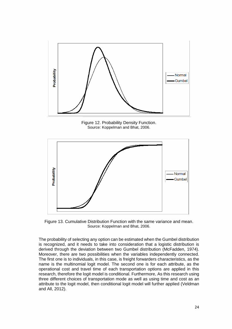
24

Figure 12. Probability Density Function. Source: Koppelman and Bhat, 2006.

Figure 13. Cumulative Distribution Function with the same variance and mean. Source: Koppelman and Bhat, 2006.

The probability of selecting any option can be estimated when the Gumbel distribution is recognized, and it needs to take into consideration that a logistic distribution is derived through the deviation between two Gumbel distribution (McFadden, 1974). Moreover, there are two possibilities when the variables independently connected. The first one is to individuals, in this case, is freight forwarders characteristics, as the name is the multinomial logit model. The second one is for each attribute, as the operational cost and travel time of each transportation options are applied in this research, therefore the logit model is conditional. Furthermore, As this research using three different choices of transportation mode as well as using time and cost as an attribute to the logit model, then conditional logit model will further applied (Veldman and All, 2012).

25

The logit model formula is described by Ortuzar and Willumsen (1990) in the transportation handbooks. The probability of choosing modal i for shipper j can be expressed as :

𝑃𝑖 =

𝑒𝑈𝑖

∑ 𝑒𝑈𝑘𝑘=𝐼𝑘=1

(1)

Where :

𝑃𝑖 : The Probability of choosing a certain transportation mode i from all possible ones i = 1...I

𝑈𝑖 : The ‘utility’ attached to mode i k : Index of mode

The probability function above is applied for all cargos transported over the route of Jakarta to Surabaya and vice versa. It is also applied to the one type of shipper which is categorized as freight forwarders that have cargo shipments in the corridor of Jakarta – Surabaya. The probability of Pi can be interpreted as the market share of the shippers or freight forwarders using mode i among all the transportation mode provided in the certain route.

In the case of this study the choices are divided into three kinds of transportation mode:

1. Truck Transport (T): Container carried only by truck from the origin to destination place.

2. Multimodal Rail Transport (R): Container is picked up from the origin location to loading rail station and from unloading rail station to a destination point by truck. Meanwhile, the railway transport is employed between the two stations.

3. Multimodal Sea Transport (S): Container is picked up from the origin location to port of loading and from port of unloading to a destination point by truck, meanwhile short sea shipping transport is employed between the two seaports.

Then the probability function will come into three equations for assessing the market share of individual transportation mode as follow:

𝑃𝑇 =

𝑒𝑈𝑇

𝑒𝑈𝑇 + 𝑒𝑈𝑅+𝑒𝑈𝑆

(2)

𝑃𝑅 =𝑒𝑈𝑅

𝑒𝑈𝑇 + 𝑒𝑈𝑅+𝑒𝑈𝑆

(3)

𝑃𝑆 =𝑒𝑈𝑆

𝑒𝑈𝑇 + 𝑒𝑈𝑅+𝑒𝑈𝑆

(4)

As the main objective is assessing the potential market share of short sea shipping, the function of Ps or probability function of multimodal sea transport would be the main focus of this research. However, It is also worth to take a note of the shift of the truck and rail’s market share as the impact of the entrance of the new modal option.

The value in which a freight forwarder attaches to the certain transportation mode m is determined in the utility. The utility of a truck, railroad and sea are expressed in Ut,

26

Ur, Us respectively. It is defined as a linear combination of all attributes which commonly has an impact on the decision makers to choose the particular option. Operational cost and delivery time are considered as the majority of crucial aspect whereby freight forwarders have to think multiple times before coming to the decision. Accordingly, in this research, those two attributes are chosen as part of the shipper’s utility function, the utility formula is expressed as :

𝑈𝑖 = 𝛼0𝐷𝑖 + 𝛼1𝐶𝑖 + 𝛼2𝑇𝑖 (5)

Where :

𝐷𝑖 : Dummy variable as an indicator that the freight forwarders have a preference on the transportation mode i

𝐶𝑖 : Total operational door-to-door cost of transportation mode i in the certain route

𝑇𝑖 : Delivery time of door-to-door service by the transportation mode i through the chosen route

𝛼0, 𝛼1, 𝛼2: The coefficients of the utility function.

Accordingly, the three utility functions for three different transportation mode are generated as follows :

𝑈𝑇 = 𝛼0𝐷𝑇 + 𝛼1𝐶𝑇 + 𝛼2𝑇𝑇 (6) 𝑈𝑅 = 𝛼0𝐷𝑅 + 𝛼1𝐶𝑅 + 𝛼2𝑇𝑅 (7) 𝑈𝑆 = 𝛼0𝐷𝑆 + 𝛼1𝐶𝑆 + 𝛼2𝑇𝑆 (8)

3.2. Stated preference analysis for coefficient of utility function

The coefficient of the utility function is the subjective values in each attribute, such as the value of cost and value of time, which is revealed by the freight forwarders. The value of the coefficient can be deduced through conducting stated preference analysis. Stated preference analysis is commonly employed on the occasion of the choice option made which doesn’t exist yet. It can be said that the interviewers state their preferences over their choice under the experimental condition.

This research ideally should have conducted the interview to the number of freight forwarders which have shipments from Jakarta to Surabaya and vice versa. Unfortunately, for the reason of the time constraint of this thesis research that is only two months period, and another reason, Indonesian freight forwarders are not quite familiar using video conference, then the secondary sources need to be consulted.

Veldman (1994) studied the application of logit model for port choice in container shipping. The research briefly compares the two different options of transportation mode in order to move the imported goods from Hamburg to the several locations in Poland. The object of the research was shippers or freight forwarders who will carry the container from Hamburg to Poland. Firstly, the scenario is forwarding the container through the roadway, as trucking is the option he made, from the container terminal in Hamburg directly to the several cities in Poland. Secondly, he proposed the multimodal carriage including feeder shipping along the north sea – baltic sea route which is discharging in Gdynia port and then using trucking mode to the destination

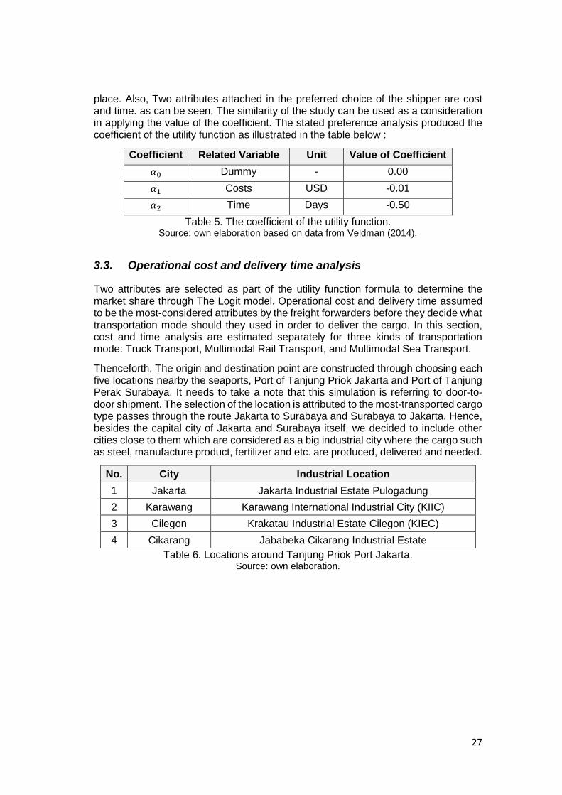
27

place. Also, Two attributes attached in the preferred choice of the shipper are cost and time. as can be seen, The similarity of the study can be used as a consideration in applying the value of the coefficient. The stated preference analysis produced the coefficient of the utility function as illustrated in the table below :

Coefficient Related Variable Unit Value of Coefficient

𝛼0 Dummy - 0.00

𝛼1 Costs USD -0.01

𝛼2 Time Days -0.50

Table 5. The coefficient of the utility function. Source: own elaboration based on data from Veldman (2014).

3.3. Operational cost and delivery time analysis

Two attributes are selected as part of the utility function formula to determine the market share through The Logit model. Operational cost and delivery time assumed to be the most-considered attributes by the freight forwarders before they decide what transportation mode should they used in order to deliver the cargo. In this section, cost and time analysis are estimated separately for three kinds of transportation mode: Truck Transport, Multimodal Rail Transport, and Multimodal Sea Transport.

Thenceforth, The origin and destination point are constructed through choosing each five locations nearby the seaports, Port of Tanjung Priok Jakarta and Port of Tanjung Perak Surabaya. It needs to take a note that this simulation is referring to door-to-door shipment. The selection of the location is attributed to the most-transported cargo type passes through the route Jakarta to Surabaya and Surabaya to Jakarta. Hence, besides the capital city of Jakarta and Surabaya itself, we decided to include other cities close to them which are considered as a big industrial city where the cargo such as steel, manufacture product, fertilizer and etc. are produced, delivered and needed.

No. City Industrial Location

1 Jakarta Jakarta Industrial Estate Pulogadung

2 Karawang Karawang International Industrial City (KIIC)

3 Cilegon Krakatau Industrial Estate Cilegon (KIEC)

4 Cikarang Jababeka Cikarang Industrial Estate

Table 6. Locations around Tanjung Priok Port Jakarta. Source: own elaboration.

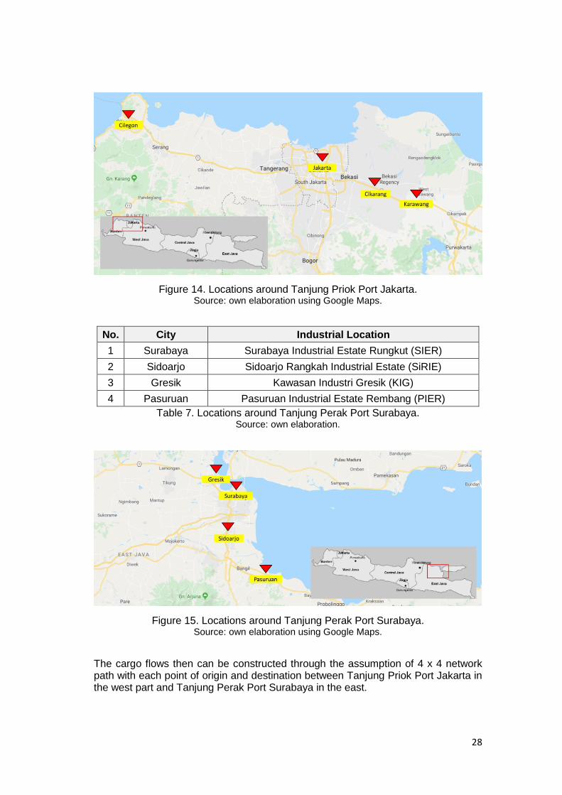
28

Figure 14. Locations around Tanjung Priok Port Jakarta. Source: own elaboration using Google Maps.

No. City Industrial Location

1 Surabaya Surabaya Industrial Estate Rungkut (SIER)

2 Sidoarjo Sidoarjo Rangkah Industrial Estate (SiRIE)

3 Gresik Kawasan Industri Gresik (KIG)

4 Pasuruan Pasuruan Industrial Estate Rembang (PIER)

Table 7. Locations around Tanjung Perak Port Surabaya. Source: own elaboration.

Figure 15. Locations around Tanjung Perak Port Surabaya. Source: own elaboration using Google Maps.

The cargo flows then can be constructed through the assumption of 4 x 4 network path with each point of origin and destination between Tanjung Priok Port Jakarta in the west part and Tanjung Perak Port Surabaya in the east.

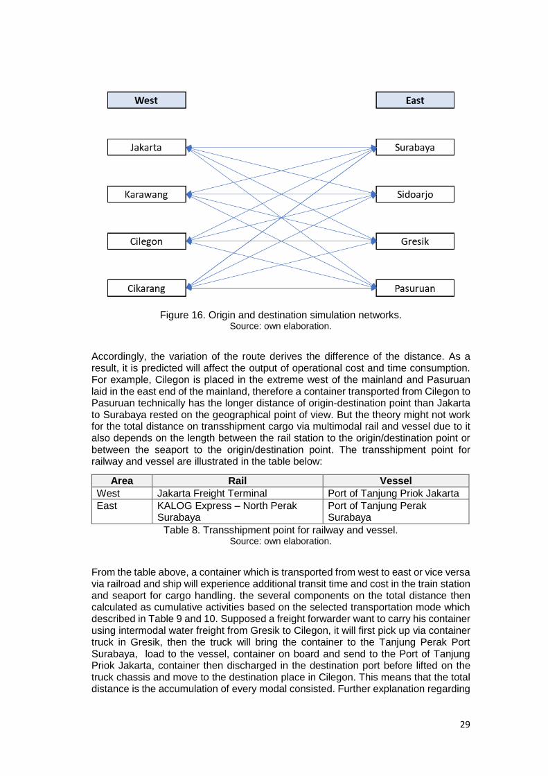
29

Figure 16. Origin and destination simulation networks. Source: own elaboration.

Accordingly, the variation of the route derives the difference of the distance. As a result, it is predicted will affect the output of operational cost and time consumption. For example, Cilegon is placed in the extreme west of the mainland and Pasuruan laid in the east end of the mainland, therefore a container transported from Cilegon to Pasuruan technically has the longer distance of origin-destination point than Jakarta to Surabaya rested on the geographical point of view. But the theory might not work for the total distance on transshipment cargo via multimodal rail and vessel due to it also depends on the length between the rail station to the origin/destination point or between the seaport to the origin/destination point. The transshipment point for railway and vessel are illustrated in the table below:

Area Rail Vessel

West Jakarta Freight Terminal Port of Tanjung Priok Jakarta

East KALOG Express – North Perak Surabaya

Port of Tanjung Perak Surabaya

Table 8. Transshipment point for railway and vessel. Source: own elaboration.

From the table above, a container which is transported from west to east or vice versa via railroad and ship will experience additional transit time and cost in the train station and seaport for cargo handling. the several components on the total distance then calculated as cumulative activities based on the selected transportation mode which described in Table 9 and 10. Supposed a freight forwarder want to carry his container using intermodal water freight from Gresik to Cilegon, it will first pick up via container truck in Gresik, then the truck will bring the container to the Tanjung Perak Port Surabaya, load to the vessel, container on board and send to the Port of Tanjung Priok Jakarta, container then discharged in the destination port before lifted on the truck chassis and move to the destination place in Cilegon. This means that the total distance is the accumulation of every modal consisted. Further explanation regarding

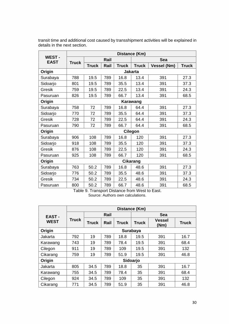
30

transit time and additional cost caused by transshipment activities will be explained in details in the next section.

WEST - EAST

Distance (Km)

Truck Rail Sea

Truck Rail Truck Truck Vessel (Nm) Truck

Origin Jakarta

Surabaya 788 19.5 789 16.8 13.4 391 27.3

Sidoarjo 801 19.5 789 35.5 13.4 391 37.3

Gresik 759 19.5 789 22.5 13.4 391 24.3

Pasuruan 826 19.5 789 66.7 13.4 391 68.5

Origin Karawang

Surabaya 758 72 789 16.8 64.4 391 27.3

Sidoarjo 770 72 789 35.5 64.4 391 37.3

Gresik 728 72 789 22.5 64.4 391 24.3

Pasuruan 790 72 789 66.7 64.4 391 68.5

Origin Cilegon

Surabaya 906 108 789 16.8 120 391 27.3

Sidoarjo 918 108 789 35.5 120 391 37.3

Gresik 876 108 789 22.5 120 391 24.3

Pasuruan 925 108 789 66.7 120 391 68.5

Origin Cikarang

Surabaya 763 50.2 789 16.8 48.6 391 27.3

Sidoarjo 776 50.2 789 35.5 48.6 391 37.3

Gresik 734 50.2 789 22.5 48.6 391 24.3

Pasuruan 800 50.2 789 66.7 48.6 391 68.5

Table 9. Transport Distance from West to East. Source: Authors own calculations.

EAST - WEST

Distance (Km)

Truck

Rail Sea

Truck Rail Truck Truck Vessel (Nm)

Truck

Origin Surabaya

Jakarta 792 19 789 18.8 19.5 391 16.7

Karawang 743 19 789 78.4 19.5 391 68.4

Cilegon 911 19 789 109 19.5 391 132

Cikarang 759 19 789 51.9 19.5 391 46.8

Origin Sidoarjo

Jakarta 805 34.5 789 18.8 35 391 16.7

Karawang 755 34.5 789 78.4 35 391 68.4

Cilegon 924 34.5 789 109 35 391 132

Cikarang 771 34.5 789 51.9 35 391 46.8

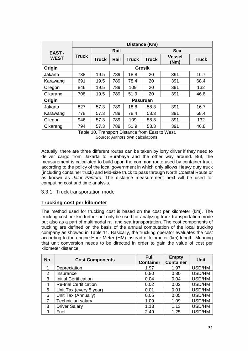
31

EAST - WEST

Distance (Km)

Truck

Rail Sea

Truck Rail Truck Truck Vessel (Nm)

Truck

Origin Gresik

Jakarta 738 19.5 789 18.8 20 391 16.7

Karawang 691 19.5 789 78.4 20 391 68.4

Cilegon 846 19.5 789 109 20 391 132

Cikarang 708 19.5 789 51.9 20 391 46.8

Origin Pasuruan

Jakarta 827 57.3 789 18.8 58.3 391 16.7

Karawang 778 57.3 789 78.4 58.3 391 68.4

Cilegon 946 57.3 789 109 58.3 391 132

Cikarang 794 57.3 789 51.9 58.3 391 46.8

Table 10. Transport Distance from East to West. Source: Authors own calculations.

Actually, there are three different routes can be taken by lorry driver if they need to deliver cargo from Jakarta to Surabaya and the other way around. But, the measurement is calculated to build upon the common route used by container truck according to the policy of the local government in which only allows Heavy duty truck (including container truck) and Mid-size truck to pass through North Coastal Route or as known as Jalur Pantura. The distance measurement next will be used for computing cost and time analysis.

3.3.1. Truck transportation mode

Trucking cost per kilometer

The method used for trucking cost is based on the cost per kilometer (km). The trucking cost per km further not only be used for analyzing truck transportation mode but also as a part of multimodal rail and sea transportation. The cost components of trucking are defined on the basis of the annual computation of the local trucking company as showed in Table 11. Basically, the trucking operator evaluates the cost according to the engine Hour Meter (HM) instead of kilometer (km) length. Meaning that unit conversion needs to be directed in order to gain the value of cost per kilometer distance.

No. Cost Components Full

Container Empty

Container Unit

1 Depreciation 1.97 1.97 USD/HM

2 Insurance 0.80 0.80 USD/HM

3 Initial Certification 0.04 0.04 USD/HM

4 Re-trial Certification 0.02 0.02 USD/HM

5 Unit Tax (every 5 year) 0.01 0.01 USD/HM

6 Unit Tax (Annually) 0.05 0.05 USD/HM

7 Technician salary 1.09 1.09 USD/HM

8 Driver Salary 1.13 1.13 USD/HM

9 Fuel 2.49 1.25 USD/HM

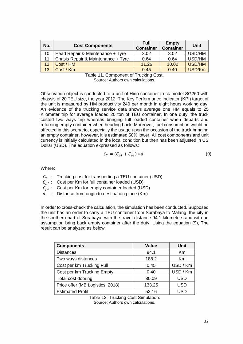
32

No. Cost Components Full

Container Empty

Container Unit

10 Head Repair & Maintenance + Tyre 3.02 3.02 USD/HM

11 Chasis Repair & Maintenance + Tyre 0.64 0.64 USD/HM

12 Cost / HM 11.26 10.02 USD/HM

13 Cost / Km 0.45 0.40 USD/Km

Table 11. Component of Trucking Cost. Source: Authors own calculations.

Observation object is conducted to a unit of Hino container truck model SG260 with chassis of 20 TEU size, the year 2012. The Key Performance Indicator (KPI) target of the unit is measured by HM productivity 240 per month in eight hours working day. An evidence of the trucking service data shows average one HM equals to 25 Kilometer trip for average loaded 20 ton of TEU container. In one duty, the truck costed two ways trip whereas bringing full loaded container when departs and returning empty container when heading back. Moreover, fuel consumption would be affected in this scenario, especially the usage upon the occasion of the truck bringing an empty container, however, it is estimated 50% lower. All cost components and unit currency is initially calculated in the local condition but then has been adjusted in US Dollar (USD). The equation expressed as follows:

𝐶𝑇 = (𝐶𝑝𝑓 + 𝐶𝑝𝑒) ∗ 𝑑 (9)

Where:

𝐶𝑇 : Trucking cost for transporting a TEU container (USD)

𝐶𝑝𝑓 : Cost per Km for full container loaded (USD)

𝐶𝑝𝑒 : Cost per Km for empty container loaded (USD)

𝑑 : Distance from origin to destination place (Km)

In order to cross-check the calculation, the simulation has been conducted. Supposed the unit has an order to carry a TEU container from Surabaya to Malang, the city in the southern part of Surabaya, with the travel distance 94.1 kilometers and with an assumption bring back empty container after the duty. Using the equation (9), The result can be analyzed as below:

Components Value Unit

Distances 94.1 Km

Two ways distances 188.2 Km

Cost per km Trucking Full 0.45 USD / Km

Cost per km Trucking Empty 0.40 USD / Km

Total cost dooring 80.09 USD

Price offer (MB Logistics, 2018) 133.25 USD

Estimated Profit 53.16 USD

Table 12. Trucking Cost Simulation. Source: Authors own calculations.

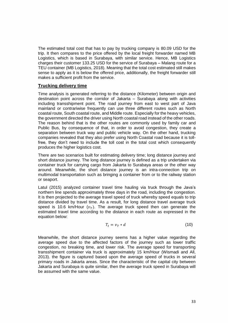
33

The estimated total cost that has to pay by trucking company is 80.09 USD for the trip. It then compares to the price offered by the local freight forwarder named MB Logistics, which is based in Surabaya, with similar service. Hence, MB Logistics charges their customer 133.25 USD for the service of Surabaya – Malang route for a TEU container (MB Logistics, 2018). Meaning that the total cost estimated still makes sense to apply as it is below the offered price, additionally, the freight forwarder still makes a sufficient profit from the service.

Trucking delivery time

Time analysis is generated referring to the distance (Kilometer) between origin and destination point across the corridor of Jakarta – Surabaya along with activities including transshipment point. The road journey from east to west part of Java mainland or contrariwise frequently can use three different routes such as North coastal route, South coastal route, and Middle route. Especially for the heavy vehicles, the government directed the driver using North coastal road instead of the other roads. The reason behind that is the other routes are commonly used by family car and Public Bus, by consequence of that, in order to avoid congestion, they create a separation between truck way and public vehicle way. On the other hand, trucking companies revealed that they also prefer using North Coastal road because it is toll-free, they don’t need to include the toll cost in the total cost which consequently produces the higher logistics cost.

There are two scenarios built for estimating delivery time; long distance journey and short distance journey. The long distance journey is defined as a trip undertaken via container truck for carrying cargo from Jakarta to Surabaya areas or the other way around. Meanwhile, the short distance journey is an intra-connection trip on multimodal transportation such as bringing a container from or to the railway station or seaport.

Latul (2015) analyzed container travel time hauling via truck through the Java’s northern line spends approximately three days in the road, including the congestion. It is then projected to the average travel speed of truck whereby speed equals to trip distance divided by travel time. As a result, for long distance travel average truck speed is 10.6 km/Hour (𝑣𝑇). The average truck speed then can generate the estimated travel time according to the distance in each route as expressed in the equation below:

𝑇𝑡 = 𝑣𝑇 ∗ 𝑑 (10)

Meanwhile, the short distance journey seems has a higher value regarding the average speed due to the affected factors of the journey such as lower traffic congestion, no breaking time, and lower risk. The average speed for transporting transshipment container via truck is approximately 15 km/Hour (Wismadi and All, 2013). the figure is captured based upon the average speed of trucks in several primary roads in Jakarta areas. Since the characteristic of the capital city between Jakarta and Surabaya is quite similar, then the average truck speed in Surabaya will be assumed with the same value.

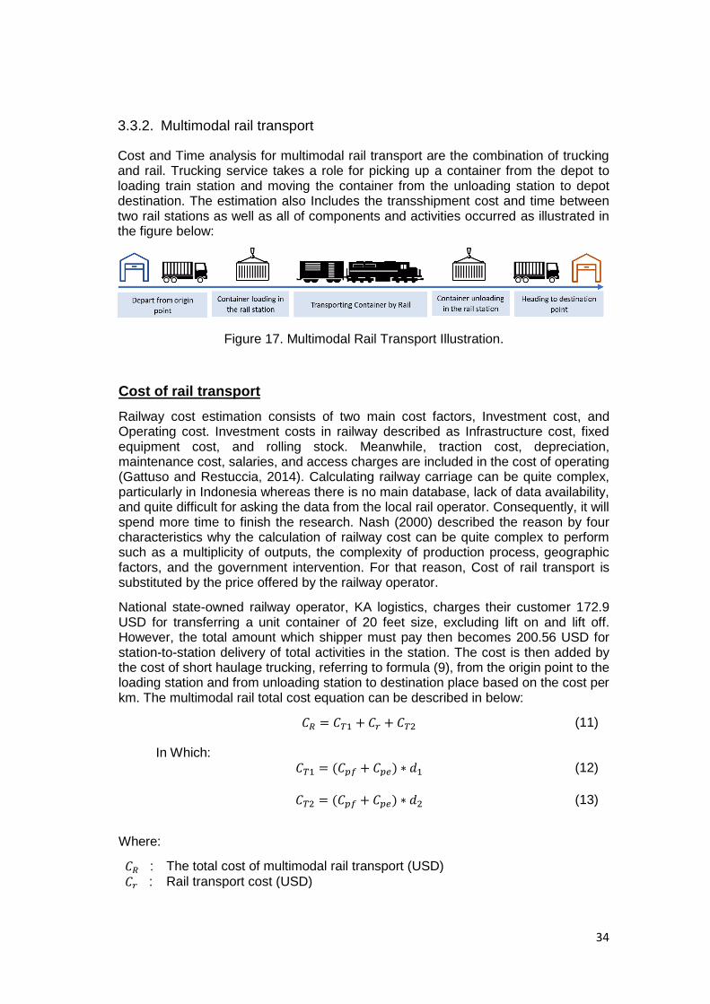
34

3.3.2. Multimodal rail transport

Cost and Time analysis for multimodal rail transport are the combination of trucking and rail. Trucking service takes a role for picking up a container from the depot to loading train station and moving the container from the unloading station to depot destination. The estimation also Includes the transshipment cost and time between two rail stations as well as all of components and activities occurred as illustrated in the figure below:

Figure 17. Multimodal Rail Transport Illustration.

Cost of rail transport

Railway cost estimation consists of two main cost factors, Investment cost, and Operating cost. Investment costs in railway described as Infrastructure cost, fixed equipment cost, and rolling stock. Meanwhile, traction cost, depreciation, maintenance cost, salaries, and access charges are included in the cost of operating (Gattuso and Restuccia, 2014). Calculating railway carriage can be quite complex, particularly in Indonesia whereas there is no main database, lack of data availability, and quite difficult for asking the data from the local rail operator. Consequently, it will spend more time to finish the research. Nash (2000) described the reason by four characteristics why the calculation of railway cost can be quite complex to perform such as a multiplicity of outputs, the complexity of production process, geographic factors, and the government intervention. For that reason, Cost of rail transport is substituted by the price offered by the railway operator.

National state-owned railway operator, KA logistics, charges their customer 172.9 USD for transferring a unit container of 20 feet size, excluding lift on and lift off. However, the total amount which shipper must pay then becomes 200.56 USD for station-to-station delivery of total activities in the station. The cost is then added by the cost of short haulage trucking, referring to formula (9), from the origin point to the loading station and from unloading station to destination place based on the cost per km. The multimodal rail total cost equation can be described in below:

𝐶𝑅 = 𝐶𝑇1 + 𝐶𝑟 + 𝐶𝑇2 (11)

In Which: 𝐶𝑇1 = (𝐶𝑝𝑓 + 𝐶𝑝𝑒) ∗ 𝑑1 (12)

𝐶𝑇2 = (𝐶𝑝𝑓 + 𝐶𝑝𝑒) ∗ 𝑑2 (13)

Where:

𝐶𝑅 : The total cost of multimodal rail transport (USD)

𝐶𝑟 : Rail transport cost (USD)

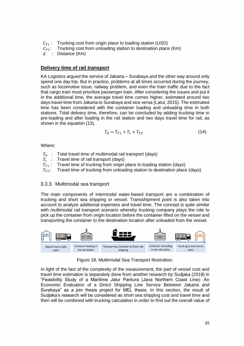
35

𝐶𝑇1 : Trucking cost from origin place to loading station (USD)

𝐶𝑇2: Trucking cost from unloading station to destination place (Km)

𝑑 : Distance (Km)

Delivery time of rail transport

KA Logistics argued the service of Jakarta – Surabaya and the other way around only spend one day trip. But in practice, problems at all times occurred during the journey, such as locomotive issue, railway problem, and even the train traffic due to the fact that cargo train must prioritize passenger train. After considering the issues and put it in the additional time, the average travel time comes higher, estimated around two days travel time from Jakarta to Surabaya and vice versa (Latul, 2015). The estimated time has been considered with the container loading and unloading time in both stations. Total delivery time, therefore, can be concluded by adding trucking time in pre-loading and after loading in the rail station and two days travel time for rail, as shown in the equation (13).

𝑇𝑅 = 𝑇𝑇1 + 𝑇𝑟 + 𝑇𝑇2 (14)

Where:

𝑇𝑅 : Total travel time of multimodal rail transport (days)

𝑇𝑟 : Travel time of rail transport (days)

𝑇𝑇1 : Travel time of trucking from origin place to loading station (days)

𝑇𝑇2: Travel time of trucking from unloading station to destination place (days)

3.3.3. Multimodal sea transport

The main components of intermodal water-based transport are a combination of trucking and short sea shipping or vessel. Transshipment point is also taken into account to analyze additional expenses and travel time. The concept is quite similar with multimodal rail transport scenario whereby trucking company plays the role to pick up the container from origin location before the container lifted on the vessel and transporting the container to the destination location after unloaded from the vessel.

Figure 18. Multimodal Sea Transport Illustration.

In light of the fact of the complexity of the measurement, the part of vessel cost and travel time estimation is separately done from another research by Sudjaka (2018) in “Feasibility Study of a Maritime Jalur Pantura (Java Northern Coast Line): An Economic Evaluation of a Direct Shipping Line Service Between Jakarta and Surabaya” as a join thesis project for MEL thesis. In this section, the result of Sudjaka’s research will be considered as short sea shipping cost and travel time and then will be combined with trucking calculation in order to find out the overall value of

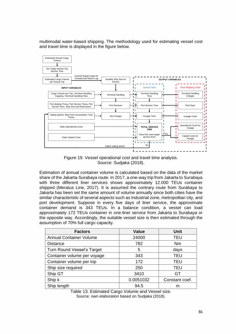
36

multimodal water-based shipping. The methodology used for estimating vessel cost and travel time is displayed in the figure below.

Figure 19. Vessel operational cost and travel time analysis. Source: Sudjaka (2018).

Estimation of annual container volume is calculated based on the data of the market share of the Jakarta-Surabaya route. In 2017, a one-way trip from Jakarta to Surabaya with three different liner services shows approximately 12.000 TEUs container shipped (Meratus Line, 2017). It is assumed the contrary route from Surabaya to Jakarta has been set the same amount of volume annually since both cities have the similar characteristic of several aspects such as Industrial zone, metropolitan city, and port development. Suppose in every five days of liner service, the approximate container demand is 343 TEUs. In a balance condition, a vessel can load approximately 172 TEUs container in one-liner service from Jakarta to Surabaya or the opposite way. Accordingly, the suitable vessel size is then estimated through the assumption of 70% full cargo capacity.

Factors Value Unit

Annual Container Volume 24000 TEU

Distance 782 Nm

Turn Round Vessel’s Target 5 days

Container volume per voyage 343 TEU

Container volume per trip 172 TEU

Ship size required 250 TEU

Ship GT 3410 GT

Ship k 0.0051032 Constant coef.

Ship length 94.5 m

Table 13. Estimated Cargo Volume and Vessel size. Source: own elaboration based on Sudjaka (2018).

Estimated Annual Cargo Volume

Set Target Round-Trip Service Time

Estimated Cargo Volume per Round-Trip

Suitable Ship Size for Service

Assume Equal Cargo for Forward and Return Leg

Terminal Handling

INPUT VARIABLES

Cargo Volume per Trip, Terminal Handling Capacity, Terminal Handling Fees

Port Services Port Waiting Times, Port Service Times, Port

Service Fees, Ship Size and Dimensions

Sea Voyage Sailing Speed, Ship Fuel Consumption, Fuel

Prices

Total Shipping Costs Service Time

Terminal Handling Time

Port Service Time

Voyage Time

Terminal Handling Charges

Port Dues

Voyage Costs

Daily Operational Costs

Daily Capital Costs

TOTAL SERVICE TIME

Does this meet target

service time?

Adjust sailing speed

Operational Costs for Voyage

Capital Costs for Voyage

No

Yes

OUTPUT VARIABLES

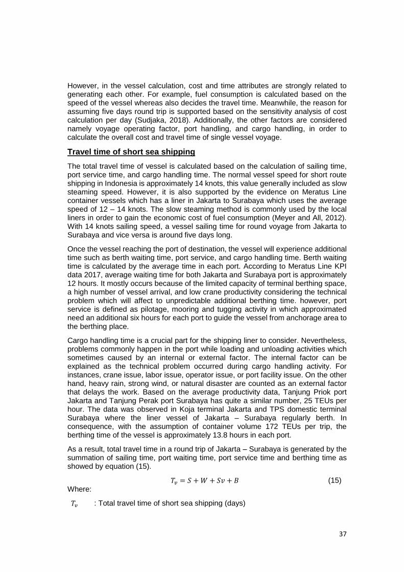
37

However, in the vessel calculation, cost and time attributes are strongly related to generating each other. For example, fuel consumption is calculated based on the speed of the vessel whereas also decides the travel time. Meanwhile, the reason for assuming five days round trip is supported based on the sensitivity analysis of cost calculation per day (Sudjaka, 2018). Additionally, the other factors are considered namely voyage operating factor, port handling, and cargo handling, in order to calculate the overall cost and travel time of single vessel voyage.

Travel time of short sea shipping

The total travel time of vessel is calculated based on the calculation of sailing time, port service time, and cargo handling time. The normal vessel speed for short route shipping in Indonesia is approximately 14 knots, this value generally included as slow steaming speed. However, it is also supported by the evidence on Meratus Line container vessels which has a liner in Jakarta to Surabaya which uses the average speed of 12 – 14 knots. The slow steaming method is commonly used by the local liners in order to gain the economic cost of fuel consumption (Meyer and All, 2012). With 14 knots sailing speed, a vessel sailing time for round voyage from Jakarta to Surabaya and vice versa is around five days long.

Once the vessel reaching the port of destination, the vessel will experience additional time such as berth waiting time, port service, and cargo handling time. Berth waiting time is calculated by the average time in each port. According to Meratus Line KPI data 2017, average waiting time for both Jakarta and Surabaya port is approximately 12 hours. It mostly occurs because of the limited capacity of terminal berthing space, a high number of vessel arrival, and low crane productivity considering the technical problem which will affect to unpredictable additional berthing time. however, port service is defined as pilotage, mooring and tugging activity in which approximated need an additional six hours for each port to guide the vessel from anchorage area to the berthing place.

Cargo handling time is a crucial part for the shipping liner to consider. Nevertheless, problems commonly happen in the port while loading and unloading activities which sometimes caused by an internal or external factor. The internal factor can be explained as the technical problem occurred during cargo handling activity. For instances, crane issue, labor issue, operator issue, or port facility issue. On the other hand, heavy rain, strong wind, or natural disaster are counted as an external factor that delays the work. Based on the average productivity data, Tanjung Priok port Jakarta and Tanjung Perak port Surabaya has quite a similar number, 25 TEUs per hour. The data was observed in Koja terminal Jakarta and TPS domestic terminal Surabaya where the liner vessel of Jakarta – Surabaya regularly berth. In consequence, with the assumption of container volume 172 TEUs per trip, the berthing time of the vessel is approximately 13.8 hours in each port.

As a result, total travel time in a round trip of Jakarta – Surabaya is generated by the summation of sailing time, port waiting time, port service time and berthing time as showed by equation (15).

𝑇𝑣 = 𝑆 +𝑊 + 𝑆𝑣 + 𝐵 (15)

Where:

𝑇𝑣 : Total travel time of short sea shipping (days)

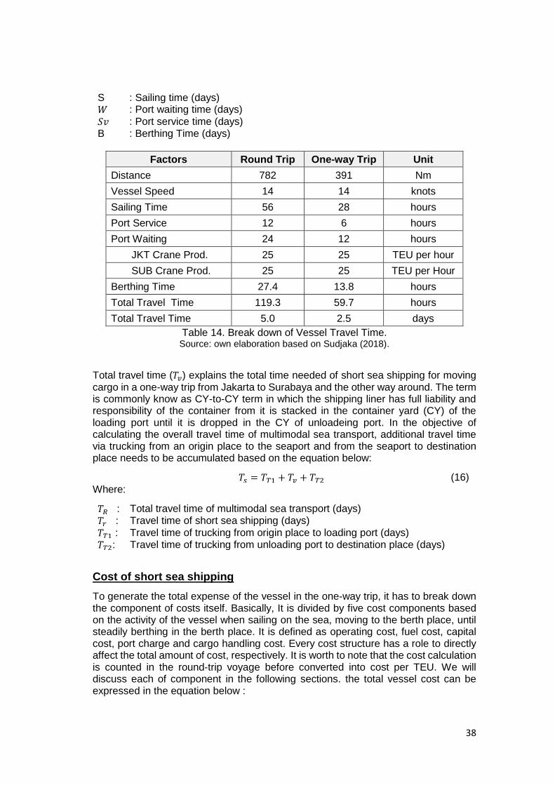
38

S : Sailing time (days) 𝑊 : Port waiting time (days)

𝑆𝑣 : Port service time (days) B : Berthing Time (days)

Factors Round Trip One-way Trip Unit

Distance 782 391 Nm

Vessel Speed 14 14 knots

Sailing Time 56 28 hours

Port Service 12 6 hours

Port Waiting 24 12 hours

JKT Crane Prod. 25 25 TEU per hour

SUB Crane Prod. 25 25 TEU per Hour

Berthing Time 27.4 13.8 hours

Total Travel Time 119.3 59.7 hours

Total Travel Time 5.0 2.5 days

Table 14. Break down of Vessel Travel Time. Source: own elaboration based on Sudjaka (2018).

Total travel time (𝑇𝑣) explains the total time needed of short sea shipping for moving cargo in a one-way trip from Jakarta to Surabaya and the other way around. The term is commonly know as CY-to-CY term in which the shipping liner has full liability and responsibility of the container from it is stacked in the container yard (CY) of the loading port until it is dropped in the CY of unloadeing port. In the objective of calculating the overall travel time of multimodal sea transport, additional travel time via trucking from an origin place to the seaport and from the seaport to destination place needs to be accumulated based on the equation below:

𝑇𝑠 = 𝑇𝑇1 + 𝑇𝑣 + 𝑇𝑇2 (16)

Where:

𝑇𝑅 : Total travel time of multimodal sea transport (days)

𝑇𝑟 : Travel time of short sea shipping (days)

𝑇𝑇1 : Travel time of trucking from origin place to loading port (days)

𝑇𝑇2: Travel time of trucking from unloading port to destination place (days)

Cost of short sea shipping

To generate the total expense of the vessel in the one-way trip, it has to break down the component of costs itself. Basically, It is divided by five cost components based on the activity of the vessel when sailing on the sea, moving to the berth place, until steadily berthing in the berth place. It is defined as operating cost, fuel cost, capital cost, port charge and cargo handling cost. Every cost structure has a role to directly affect the total amount of cost, respectively. It is worth to note that the cost calculation is counted in the round-trip voyage before converted into cost per TEU. We will discuss each of component in the following sections. the total vessel cost can be expressed in the equation below :

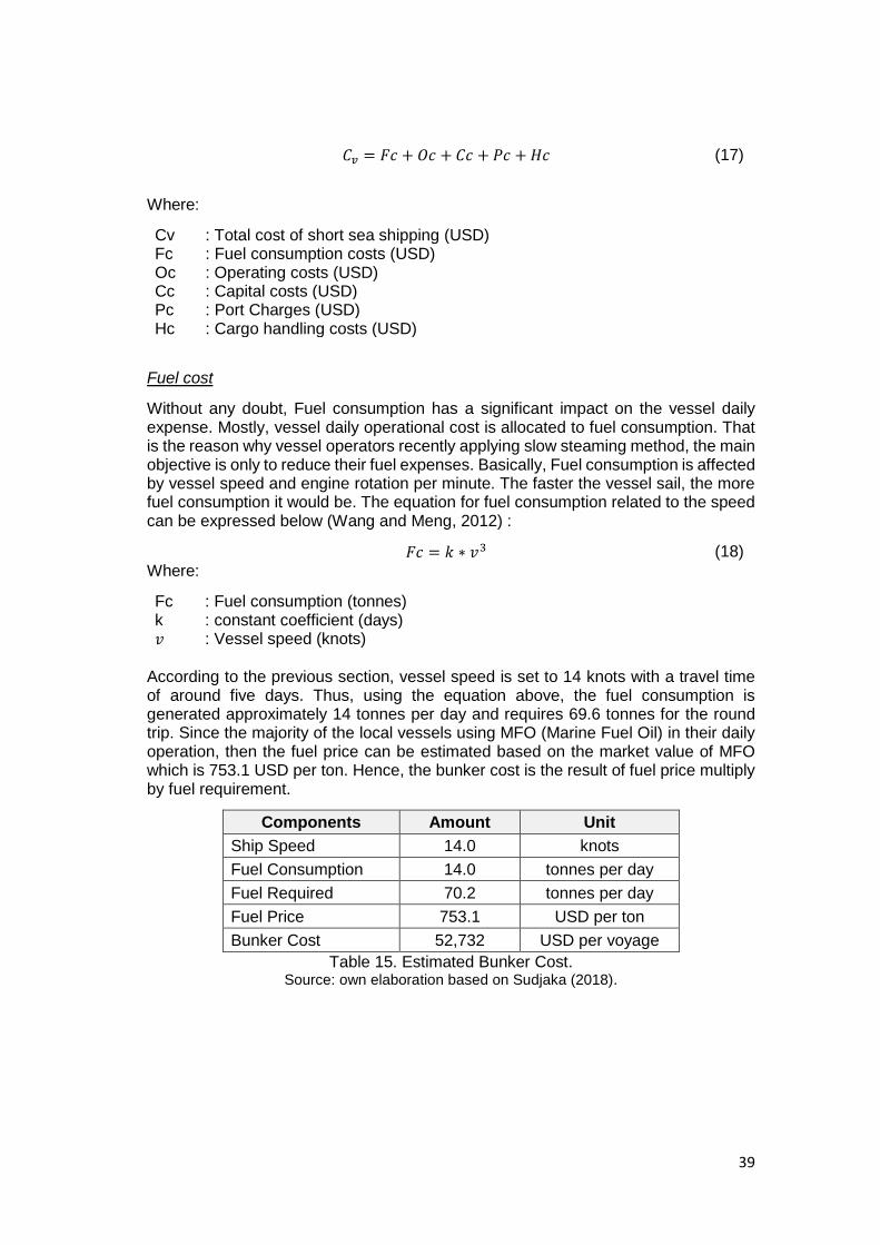
39

𝐶𝑣 = 𝐹𝑐 + 𝑂𝑐 + 𝐶𝑐 + 𝑃𝑐 + 𝐻𝑐 (17)

Where:

Cv : Total cost of short sea shipping (USD) Fc : Fuel consumption costs (USD) Oc : Operating costs (USD) Cc : Capital costs (USD) Pc : Port Charges (USD) Hc : Cargo handling costs (USD)

Fuel cost

Without any doubt, Fuel consumption has a significant impact on the vessel daily expense. Mostly, vessel daily operational cost is allocated to fuel consumption. That is the reason why vessel operators recently applying slow steaming method, the main objective is only to reduce their fuel expenses. Basically, Fuel consumption is affected by vessel speed and engine rotation per minute. The faster the vessel sail, the more fuel consumption it would be. The equation for fuel consumption related to the speed can be expressed below (Wang and Meng, 2012) :

𝐹𝑐 = 𝑘 ∗ 𝑣3 (18)

Where:

Fc : Fuel consumption (tonnes) k : constant coefficient (days) 𝑣 : Vessel speed (knots)

According to the previous section, vessel speed is set to 14 knots with a travel time of around five days. Thus, using the equation above, the fuel consumption is generated approximately 14 tonnes per day and requires 69.6 tonnes for the round trip. Since the majority of the local vessels using MFO (Marine Fuel Oil) in their daily operation, then the fuel price can be estimated based on the market value of MFO which is 753.1 USD per ton. Hence, the bunker cost is the result of fuel price multiply by fuel requirement.

Components Amount Unit

Ship Speed 14.0 knots

Fuel Consumption 14.0 tonnes per day

Fuel Required 70.2 tonnes per day

Fuel Price 753.1 USD per ton

Bunker Cost 52,732 USD per voyage

Table 15. Estimated Bunker Cost. Source: own elaboration based on Sudjaka (2018).

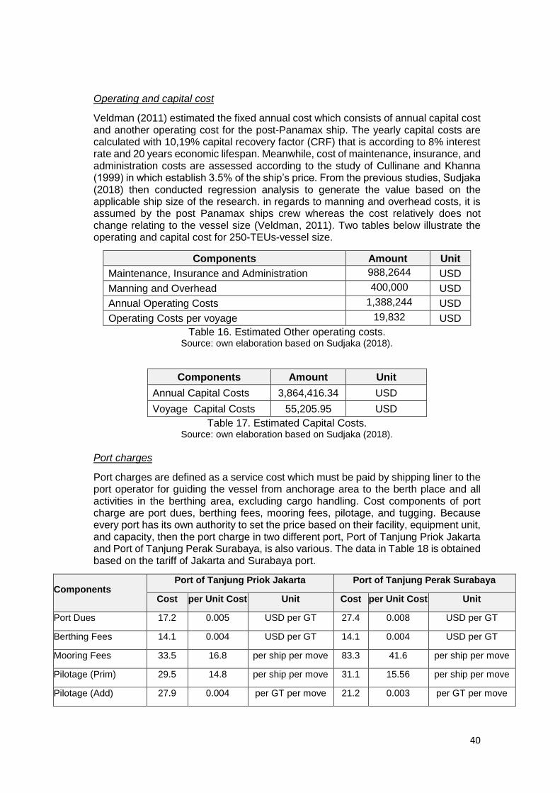
40

Operating and capital cost

Veldman (2011) estimated the fixed annual cost which consists of annual capital cost and another operating cost for the post-Panamax ship. The yearly capital costs are calculated with 10,19% capital recovery factor (CRF) that is according to 8% interest rate and 20 years economic lifespan. Meanwhile, cost of maintenance, insurance, and administration costs are assessed according to the study of Cullinane and Khanna (1999) in which establish 3.5% of the ship’s price. From the previous studies, Sudjaka (2018) then conducted regression analysis to generate the value based on the applicable ship size of the research. in regards to manning and overhead costs, it is assumed by the post Panamax ships crew whereas the cost relatively does not change relating to the vessel size (Veldman, 2011). Two tables below illustrate the operating and capital cost for 250-TEUs-vessel size.

Components Amount Unit

Maintenance, Insurance and Administration 988,2644 USD

Manning and Overhead 400,000 USD

Annual Operating Costs 1,388,244 USD

Operating Costs per voyage 19,832 USD

Table 16. Estimated Other operating costs. Source: own elaboration based on Sudjaka (2018).

Components Amount Unit

Annual Capital Costs 3,864,416.34 USD

Voyage Capital Costs 55,205.95 USD

Table 17. Estimated Capital Costs. Source: own elaboration based on Sudjaka (2018).

Port charges

Port charges are defined as a service cost which must be paid by shipping liner to the port operator for guiding the vessel from anchorage area to the berth place and all activities in the berthing area, excluding cargo handling. Cost components of port charge are port dues, berthing fees, mooring fees, pilotage, and tugging. Because every port has its own authority to set the price based on their facility, equipment unit, and capacity, then the port charge in two different port, Port of Tanjung Priok Jakarta and Port of Tanjung Perak Surabaya, is also various. The data in Table 18 is obtained based on the tariff of Jakarta and Surabaya port.

Components Port of Tanjung Priok Jakarta Port of Tanjung Perak Surabaya

Cost per Unit Cost Unit Cost per Unit Cost Unit

Port Dues 17.2 0.005 USD per GT 27.4 0.008 USD per GT

Berthing Fees 14.1 0.004 USD per GT 14.1 0.004 USD per GT

Mooring Fees 33.5 16.8 per ship per move 83.3 41.6 per ship per move

Pilotage (Prim) 29.5 14.8 per ship per move 31.1 15.56 per ship per move

Pilotage (Add) 27.9 0.004 per GT per move 21.2 0.003 per GT per move

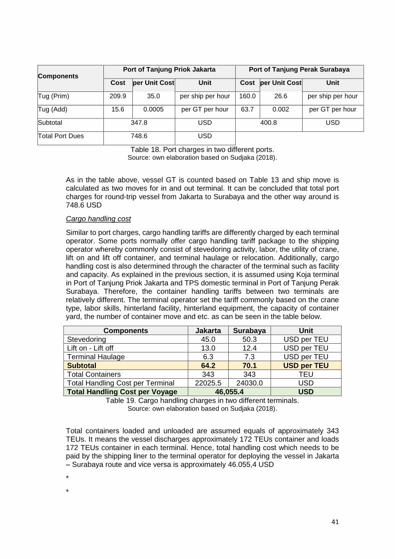
41

Components Port of Tanjung Priok Jakarta Port of Tanjung Perak Surabaya

Cost per Unit Cost Unit Cost per Unit Cost Unit

Tug (Prim) 209.9 35.0 per ship per hour 160.0 26.6 per ship per hour

Tug (Add) 15.6 0.0005 per GT per hour 63.7 0.002 per GT per hour

Subtotal 347.8 USD 400.8 USD

Total Port Dues 748.6 USD

Table 18. Port charges in two different ports. Source: own elaboration based on Sudjaka (2018).

As in the table above, vessel GT is counted based on Table 13 and ship move is calculated as two moves for in and out terminal. It can be concluded that total port charges for round-trip vessel from Jakarta to Surabaya and the other way around is 748.6 USD

Cargo handling cost

Similar to port charges, cargo handling tariffs are differently charged by each terminal operator. Some ports normally offer cargo handling tariff package to the shipping operator whereby commonly consist of stevedoring activity, labor, the utility of crane, lift on and lift off container, and terminal haulage or relocation. Additionally, cargo handling cost is also determined through the character of the terminal such as facility and capacity. As explained in the previous section, it is assumed using Koja terminal in Port of Tanjung Priok Jakarta and TPS domestic terminal in Port of Tanjung Perak Surabaya. Therefore, the container handling tariffs between two terminals are relatively different. The terminal operator set the tariff commonly based on the crane type, labor skills, hinterland facility, hinterland equipment, the capacity of container yard, the number of container move and etc. as can be seen in the table below.

Components Jakarta Surabaya Unit

Stevedoring 45.0 50.3 USD per TEU

Lift on - Lift off 13.0 12.4 USD per TEU

Terminal Haulage 6.3 7.3 USD per TEU

Subtotal 64.2 70.1 USD per TEU

Total Containers 343 343 TEU

Total Handling Cost per Terminal 22025.5 24030.0 USD

Total Handling Cost per Voyage 46,055.4 USD

Table 19. Cargo handling charges in two different terminals. Source: own elaboration based on Sudjaka (2018).

Total containers loaded and unloaded are assumed equals of approximately 343 TEUs. It means the vessel discharges approximately 172 TEUs container and loads 172 TEUs container in each terminal. Hence, total handling cost which needs to be paid by the shipping liner to the terminal operator for deploying the vessel in Jakarta – Surabaya route and vice versa is approximately 46.055,4 USD

*

*

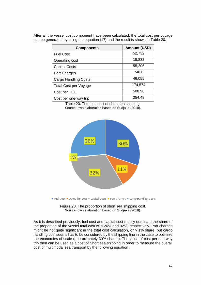
42

After all the vessel cost component have been calculated, the total cost per voyage can be generated by using the equation (17) and the result is shown in Table 20.

Components Amount (USD)

Fuel Cost 52,732

Operating cost 19,832

Capital Costs 55,206

Port Charges 748.6

Cargo Handling Costs 46,055

Total Cost per Voyage 174,574

Cost per TEU 508.96

Cost per one-way trip 254.48

Table 20. The total cost of short sea shipping. Source: own elaboration based on Sudjaka (2018).

Figure 20. The proportion of short sea shipping cost. Source: own elaboration based on Sudjaka (2018).

As it is described previously, fuel cost and capital cost mostly dominate the share of the proportion of the vessel total cost with 26% and 32%, respectively. Port charges might be not quite significant in the total cost calculation, only 1% share, but cargo handling cost seems has to be considered by the shipping line in the case to optimize the economies of scale (approximately 30% shares). The value of cost per one-way trip then can be used as a cost of Short sea shipping in order to measure the overall cost of multimodal sea transport by the following equation :

43

𝐶𝑠 = 𝐶𝑇1 + 𝐶𝑣 + 𝐶𝑇2 (19)

Where:

𝐶𝑠 : Total cost of multimodal sea transport (USD)

𝐶𝑣 : Total cost of short sea shipping (USD)

𝐶𝑇1 : Total cost of trucking from origin place to loading port (USD)

𝐶𝑇2: Total cost of trucking from unloading port to destination place (USD)

3.4. Data collection

Researches performed in Indonesia commonly struggle with the data collection. The national data center (BPS) unfortunately doesn’t present a sufficient data regarding the research. Data available for research purpose also has an issue when touching private company. Private companies barely give their personal data even though for educational purpose. However, the common issue sometimes is no sufficient data provided or the data is confidential.

Fortunately, the author was working in the local shipping company in Indonesia, named Meratus Line, in which has access to mine the data for the research purpose, even though was not quite perfect but remains applicable for this research. The data of the initial market share, the most-transported commodity, and the actual vessel and train freight rates were coming from Meratus Line database, in which, however, it is applied as calculation benchmarks and references. Moreover, cost components data of truck and door-to-door trucking tariff which were acquired from a local freight forwarder, MB logistic, were very useful in the direct trucking calculation. Moving to the railways part, Indonesian state-owned rail operator only gave a clue for rail freight and relatively inaccurate delivery time. Thus, in order to cover the issue, several research journals had been implemented as additional references, for instance, the data from Latul’s research regarding railway travel time. The data from Latul’s research was also used regarding average trucking travel time from Jakarta to Surabaya and annual container transported along the Northern Java’s route. In the case of vessel operational cost and travel time information, the study from Sudjaka is borrowed as a joint thesis project for the aim of comparing the market share of each transport option.

Unfortunately, due to the fact that the time constraint and limited technology access to reach some Indonesian freight forwarders, stated preference analysis couldn’t be directly conducted. As a replacement, the result of stated preference analysis was brought from another study which has adequately similar conditions and circumstances.

3.5. Data analysis

After all the data have been collected, the next step is simply applying the certain equations using the collected data. The data of travel distance applies with the trucking speed, according to the data of another research by Latul, using equation (10), with the purpose of obtaining the travel time of the trucking mode. On the base of the trucking velocity employed, it is used to generate the travel time of short haulage trucking by equation (12) and (13). Regardless, travel time for container train is acquired based on the data of Latul’s research (2015) and then combined with short

44

distance trucking for multimodal rail transport using the equation (14). Regarding multimodal sea transport, Equation (16) generates the multimodal sea transport consisting of short distance trucking and vessel operational time. By equation (15), the total time spent by vessel for transporting cargo belongs to four components of time: sailing time on the sea, port waiting time, port service time, and berthing time. Sailing time is calculated based on the average velocity data of the domestic liner multiplies the sailing distance. Meanwhile, port waiting time, service time and berthing time are approximated based on the average port performance data.

Similarly, operational cost data for each mode employs in each total operational cost equation. The data on trucking cost components, by MB Logistics, is generated to be trucking cost per Kilometer, and it applies to long distance and short distance trucking mode by using equation (9). Meanwhile, equation (11) applies for the cost of a railway carriage which is taken from the rail operator data, KA Logistics, with the addition of short distance trucking cost for the purpose of constructing multimodal rail transport cost. Besides, shipping cost per TEUs is earned from the total five cost components data: fuel cost, operational cost, capital cost, port charge and cargo handling cost, before summed with short distance haulage according to equation (17) in order to obtain the total cost of multimodal sea transport.

Furthermore, in respect of the equation of utility function, the coefficient of the utility function, as a result of the study by Veldman, is applied along with the result of operational cost and travel time on each transport mode. It is illustrated by equation (6), (7) and (8) for trucking, multimodal rail, and multimodal sea transport, respectively. Finally, the result of each utility function produces the market share for each transport choice using equation (2), (3), and (4). The proportion of the market share of each mode on each different route is then projected to the number of TEUs container by multiplying with the data of total container carried along the route of Jakarta – Surabaya and vice versa.

3.6. Conclusion

The conditional logit model is consulted as the ideal approach for the objective of estimating market share for three transportation choices in which one of them still doesn’t exist yet and acts as the proposed alternative. Additionally, operational cost and time analysis are as close as possible precisely structured based on the real condition of transportation modes respectively. The collected data are sufficient enough to be applied in the provided equations and models and, moreover, the data sources which are acquired from the local shipping company, freight forwarder, and various feasible transport studies, are also adequately reliable and credible to perform the equations in order to generate the output.

45

Chapter 4 Result and analysis

The research calculation is divided into four phases of analysis including operational cost, travel time, market share and potential container flows. Therefore, the analysis and explanation in this chapter are evaluated based on each calculation employed. Basically, the calculation of operational cost and travel time have to be done before coming to the estimation of the potential market share. Subsequently, the result of the potential market share is applied to develop the number of containers transported for three various modes in each possible route.

4.1. Estimated operational cost

It can be seen in Table 18 and 19 as the result of cost analysis based on the three different modes of transportation. Cost per TEUs for moving the container directly via truck is approximately more than two times bigger than the cost of multimodal rail and sea. In regard to direct trucking, applies the longer the distance between origin and destination place, the more expensive the cost would be. The cost of the train and vessel are constant in both ways since the transshipment point of rail and sea are considered at the same point but, the cost will vary regarding the pre-loading and post-unloading activities of rail and sea due to utilizing trucking service as a connection mode in which cost per km is applied. Nevertheless, there is a small cost difference between the two same origin-destination points for two different routes, for examples, transporting cost using multimodal short sea shipping from Jakarta to Surabaya is 289.1 USD, meanwhile, from Surabaya to Jakarta is 285.3 USD. On the other hand, in the same term, the substantial differences lay in the cost of direct trucking in which the truck regularly using different city route for departure and arrival. The reason behind this is sometimes the existence of a policy by the local government for the utility of the city road by heavy vehicles which is limited based on the peak time activity. Thus, Heavy vehicles in some cases cannot pass through the main road around 7-9 a.m or 5-7 p.m as well as around the Eid Fitr celebration. As consequences, the truck driver should take another route which occasionally has longer distance or even park the truck until the time has come. Indeed this issue will be counted as a loss by the freight forwarders because it effects on the increased logistics costs.

In the different point of view, as can be seen, that rail and short sea shipping by estimation have a lower cost than a truck, 283.5 USD and 339.6 USD compared to 683.7 USD, it is technically due to the concept of economies of scale. The carried capacity via rail and short sea shipping is way bigger than a truck which only can carry one TEU container in a single way. Therefore, cost per TEU of transporting container by rail and sea becomes relatively cheaper. The interesting point in this cost analysis is that the cost of the vessel has a bit bigger than rail, approximately 56.14 USD bigger, despite the fact that the carrying capacity of short sea shipping in the one-way trip is comparatively bigger than rail, 172 over 60 TEU container. It probably happens due to the cost structure of the vessel is practically more complex and has a lot of capital investment. As it is recognized that the shipping industry is considered as a high-barrier-to-entry industry because it requires high investments and capital costs. Meanwhile, it is worth to note again that the assumption has been built that the rail cost is referring to the price offered by state-owned rail operator company in which has apparently received the transport subsidy from the government in its infrastructures, services or the other sides. However, the main objective of national state-owned enterprises is not revenue oriented but more likely for public services.

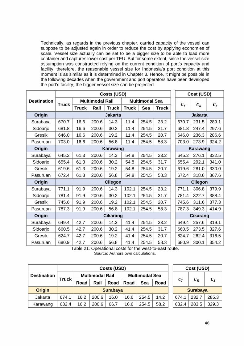
46

Technically, as regards in the previous chapter, carried capacity of the vessel can suppose to be adjusted again in order to reduce the cost by applying economies of scale. Vessel size actually can be set to be a bigger size to be able to load more container and captures lower cost per TEU. But for some extent, since the vessel size assumption was constructed relying on the current condition of port’s capacity and facility, therefore, the reasonable vessel size for Indonesia’s port condition at this moment is as similar as it is determined in Chapter 3. Hence, it might be possible in the following decades when the government and port operators have been developed the port’s facility, the bigger vessel size can be projected.

Destination

Costs (USD) Cost (USD)

Truck Multimodal Rail Multimodal Sea

𝑪𝑻 𝑪𝑹 𝑪𝑺 Truck Rail Truck Truck Sea Truck

Origin Jakarta Jakarta

Surabaya 670.7 16.6 200.6 14.3 11.4 254.5 23.2 670.7 231.5 289.1

Sidoarjo 681.8 16.6 200.6 30.2 11.4 254.5 31.7 681.8 247.4 297.6

Gresik 646.0 16.6 200.6 19.2 11.4 254.5 20.7 646.0 236.3 286.6

Pasuruan 703.0 16.6 200.6 56.8 11.4 254.5 58.3 703.0 273.9 324.2

Origin Karawang Karawang

Surabaya 645.2 61.3 200.6 14.3 54.8 254.5 23.2 645.2 276.1 332.5

Sidoarjo 655.4 61.3 200.6 30.2 54.8 254.5 31.7 655.4 292.1 341.0

Gresik 619.6 61.3 200.6 19.2 54.8 254.5 20.7 619.6 281.0 330.0

Pasuruan 672.4 61.3 200.6 56.8 54.8 254.5 58.3 672.4 318.6 367.6

Origin Cilegon Cilegon

Surabaya 771.1 91.9 200.6 14.3 102.1 254.5 23.2 771.1 306.8 379.9

Sidoarjo 781.4 91.9 200.6 30.2 102.1 254.5 31.7 781.4 322.7 388.4

Gresik 745.6 91.9 200.6 19.2 102.1 254.5 20.7 745.6 311.6 377.3

Pasuruan 787.3 91.9 200.6 56.8 102.1 254.5 58.3 787.3 349.3 414.9

Origin Cikarang Cikarang

Surabaya 649.4 42.7 200.6 14.3 41.4 254.5 23.2 649.4 257.6 319.1

Sidoarjo 660.5 42.7 200.6 30.2 41.4 254.5 31.7 660.5 273.5 327.6

Gresik 624.7 42.7 200.6 19.2 41.4 254.5 20.7 624.7 262.4 316.5

Pasuruan 680.9 42.7 200.6 56.8 41.4 254.5 58.3 680.9 300.1 354.2

Table 21. Operational costs for the west-to-east route. Source: Authors own calculations.

Destination

Costs (USD) Cost (USD)

Truck Multimodal Rail Multimodal Sea

𝑪𝑻 𝑪𝑹 𝑪𝑺 Road Rail Road Road Sea Road

Origin Surabaya Surabaya

Jakarta 674.1 16.2 200.6 16.0 16.6 254.5 14.2 674.1 232.7 285.3

Karawang 632.4 16.2 200.6 66.7 16.6 254.5 58.2 632.4 283.5 329.3

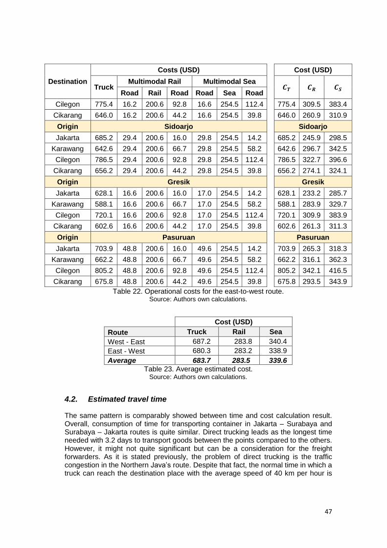
47

Destination

Costs (USD) Cost (USD)

Truck Multimodal Rail Multimodal Sea

𝑪𝑻 𝑪𝑹 𝑪𝑺 Road Rail Road Road Sea Road

Cilegon 775.4 16.2 200.6 92.8 16.6 254.5 112.4 775.4 309.5 383.4

Cikarang 646.0 16.2 200.6 44.2 16.6 254.5 39.8 646.0 260.9 310.9

Origin Sidoarjo Sidoarjo

Jakarta 685.2 29.4 200.6 16.0 29.8 254.5 14.2 685.2 245.9 298.5

Karawang 642.6 29.4 200.6 66.7 29.8 254.5 58.2 642.6 296.7 342.5

Cilegon 786.5 29.4 200.6 92.8 29.8 254.5 112.4 786.5 322.7 396.6

Cikarang 656.2 29.4 200.6 44.2 29.8 254.5 39.8 656.2 274.1 324.1

Origin Gresik Gresik

Jakarta 628.1 16.6 200.6 16.0 17.0 254.5 14.2 628.1 233.2 285.7

Karawang 588.1 16.6 200.6 66.7 17.0 254.5 58.2 588.1 283.9 329.7

Cilegon 720.1 16.6 200.6 92.8 17.0 254.5 112.4 720.1 309.9 383.9

Cikarang 602.6 16.6 200.6 44.2 17.0 254.5 39.8 602.6 261.3 311.3

Origin Pasuruan Pasuruan

Jakarta 703.9 48.8 200.6 16.0 49.6 254.5 14.2 703.9 265.3 318.3

Karawang 662.2 48.8 200.6 66.7 49.6 254.5 58.2 662.2 316.1 362.3

Cilegon 805.2 48.8 200.6 92.8 49.6 254.5 112.4 805.2 342.1 416.5

Cikarang 675.8 48.8 200.6 44.2 49.6 254.5 39.8 675.8 293.5 343.9

Table 22. Operational costs for the east-to-west route. Source: Authors own calculations.

Cost (USD)

Route Truck Rail Sea

West - East 687.2 283.8 340.4

East - West 680.3 283.2 338.9

Average 683.7 283.5 339.6

Table 23. Average estimated cost. Source: Authors own calculations.

4.2. Estimated travel time

The same pattern is comparably showed between time and cost calculation result. Overall, consumption of time for transporting container in Jakarta – Surabaya and Surabaya – Jakarta routes is quite similar. Direct trucking leads as the longest time needed with 3.2 days to transport goods between the points compared to the others. However, it might not quite significant but can be a consideration for the freight forwarders. As it is stated previously, the problem of direct trucking is the traffic congestion in the Northern Java’s route. Despite that fact, the normal time in which a truck can reach the destination place with the average speed of 40 km per hour is

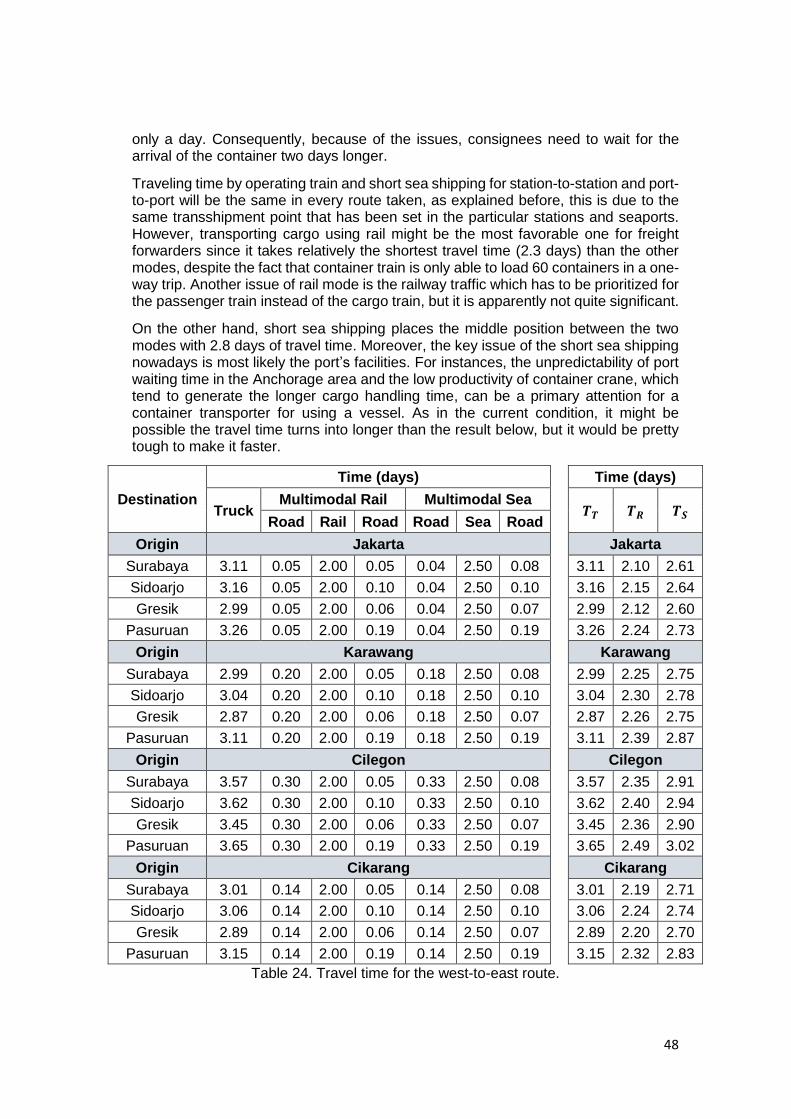
48

only a day. Consequently, because of the issues, consignees need to wait for the arrival of the container two days longer.

Traveling time by operating train and short sea shipping for station-to-station and port-to-port will be the same in every route taken, as explained before, this is due to the same transshipment point that has been set in the particular stations and seaports. However, transporting cargo using rail might be the most favorable one for freight forwarders since it takes relatively the shortest travel time (2.3 days) than the other modes, despite the fact that container train is only able to load 60 containers in a one-way trip. Another issue of rail mode is the railway traffic which has to be prioritized for the passenger train instead of the cargo train, but it is apparently not quite significant.

On the other hand, short sea shipping places the middle position between the two modes with 2.8 days of travel time. Moreover, the key issue of the short sea shipping nowadays is most likely the port’s facilities. For instances, the unpredictability of port waiting time in the Anchorage area and the low productivity of container crane, which tend to generate the longer cargo handling time, can be a primary attention for a container transporter for using a vessel. As in the current condition, it might be possible the travel time turns into longer than the result below, but it would be pretty tough to make it faster.

Destination

Time (days) Time (days)

Truck Multimodal Rail Multimodal Sea

𝑻𝑻 𝑻𝑹 𝑻𝑺 Road Rail Road Road Sea Road

Origin Jakarta Jakarta

Surabaya 3.11 0.05 2.00 0.05 0.04 2.50 0.08 3.11 2.10 2.61

Sidoarjo 3.16 0.05 2.00 0.10 0.04 2.50 0.10 3.16 2.15 2.64

Gresik 2.99 0.05 2.00 0.06 0.04 2.50 0.07 2.99 2.12 2.60

Pasuruan 3.26 0.05 2.00 0.19 0.04 2.50 0.19 3.26 2.24 2.73

Origin Karawang Karawang

Surabaya 2.99 0.20 2.00 0.05 0.18 2.50 0.08 2.99 2.25 2.75

Sidoarjo 3.04 0.20 2.00 0.10 0.18 2.50 0.10 3.04 2.30 2.78

Gresik 2.87 0.20 2.00 0.06 0.18 2.50 0.07 2.87 2.26 2.75

Pasuruan 3.11 0.20 2.00 0.19 0.18 2.50 0.19 3.11 2.39 2.87

Origin Cilegon Cilegon

Surabaya 3.57 0.30 2.00 0.05 0.33 2.50 0.08 3.57 2.35 2.91

Sidoarjo 3.62 0.30 2.00 0.10 0.33 2.50 0.10 3.62 2.40 2.94

Gresik 3.45 0.30 2.00 0.06 0.33 2.50 0.07 3.45 2.36 2.90

Pasuruan 3.65 0.30 2.00 0.19 0.33 2.50 0.19 3.65 2.49 3.02

Origin Cikarang Cikarang

Surabaya 3.01 0.14 2.00 0.05 0.14 2.50 0.08 3.01 2.19 2.71

Sidoarjo 3.06 0.14 2.00 0.10 0.14 2.50 0.10 3.06 2.24 2.74

Gresik 2.89 0.14 2.00 0.06 0.14 2.50 0.07 2.89 2.20 2.70

Pasuruan 3.15 0.14 2.00 0.19 0.14 2.50 0.19 3.15 2.32 2.83

Table 24. Travel time for the west-to-east route.

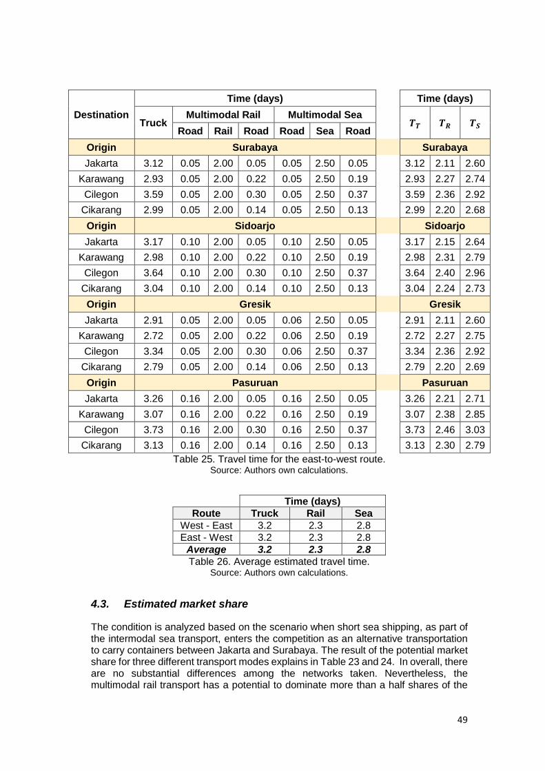
49

Destination

Time (days) Time (days)

Truck Multimodal Rail Multimodal Sea

𝑻𝑻 𝑻𝑹 𝑻𝑺 Road Rail Road Road Sea Road

Origin Surabaya Surabaya

Jakarta 3.12 0.05 2.00 0.05 0.05 2.50 0.05 3.12 2.11 2.60

Karawang 2.93 0.05 2.00 0.22 0.05 2.50 0.19 2.93 2.27 2.74

Cilegon 3.59 0.05 2.00 0.30 0.05 2.50 0.37 3.59 2.36 2.92

Cikarang 2.99 0.05 2.00 0.14 0.05 2.50 0.13 2.99 2.20 2.68

Origin Sidoarjo Sidoarjo

Jakarta 3.17 0.10 2.00 0.05 0.10 2.50 0.05 3.17 2.15 2.64

Karawang 2.98 0.10 2.00 0.22 0.10 2.50 0.19 2.98 2.31 2.79

Cilegon 3.64 0.10 2.00 0.30 0.10 2.50 0.37 3.64 2.40 2.96

Cikarang 3.04 0.10 2.00 0.14 0.10 2.50 0.13 3.04 2.24 2.73

Origin Gresik Gresik

Jakarta 2.91 0.05 2.00 0.05 0.06 2.50 0.05 2.91 2.11 2.60

Karawang 2.72 0.05 2.00 0.22 0.06 2.50 0.19 2.72 2.27 2.75

Cilegon 3.34 0.05 2.00 0.30 0.06 2.50 0.37 3.34 2.36 2.92

Cikarang 2.79 0.05 2.00 0.14 0.06 2.50 0.13 2.79 2.20 2.69

Origin Pasuruan Pasuruan

Jakarta 3.26 0.16 2.00 0.05 0.16 2.50 0.05 3.26 2.21 2.71

Karawang 3.07 0.16 2.00 0.22 0.16 2.50 0.19 3.07 2.38 2.85

Cilegon 3.73 0.16 2.00 0.30 0.16 2.50 0.37 3.73 2.46 3.03

Cikarang 3.13 0.16 2.00 0.14 0.16 2.50 0.13 3.13 2.30 2.79

Table 25. Travel time for the east-to-west route. Source: Authors own calculations.

Time (days)

Route Truck Rail Sea

West - East 3.2 2.3 2.8

East - West 3.2 2.3 2.8

Average 3.2 2.3 2.8

Table 26. Average estimated travel time. Source: Authors own calculations.

4.3. Estimated market share

The condition is analyzed based on the scenario when short sea shipping, as part of the intermodal sea transport, enters the competition as an alternative transportation to carry containers between Jakarta and Surabaya. The result of the potential market share for three different transport modes explains in Table 23 and 24. In overall, there are no substantial differences among the networks taken. Nevertheless, the multimodal rail transport has a potential to dominate more than a half shares of the

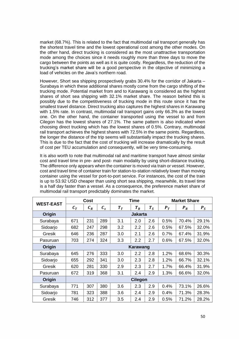
50

market (68.7%). This is related to the fact that multimodal rail transport generally has the shortest travel time and the lowest operational cost among the other modes. On the other hand, direct trucking is considered as the most unattractive transportation mode among the choices since it needs roughly more than three days to move the cargo between the points as well as it is quite costly. Regardless, the reduction of the trucking’s market share will be a good perspective in the objective of minimizing a load of vehicles on the Java’s northern road.

However, Short sea shipping prospectively grabs 30.4% for the corridor of Jakarta – Surabaya in which these additional shares mostly come from the cargo shifting of the trucking mode. Potential market from and to Karawang is considered as the highest shares of short sea shipping with 32.1% market share. The reason behind this is possibly due to the competitiveness of trucking mode in this route since it has the smallest travel distance. Direct trucking also captures the highest shares in Karawang with 1.5% rate. In contrast, multimodal rail transport gains only 66.3% as the lowest one. On the other hand, the container transported using the vessel to and from Cilegon has the lowest shares of 27.1%. The same pattern is also indicated when choosing direct trucking which has the lowest shares of 0.5%. Contrary, multimodal rail transport achieves the highest shares with 72.5% in the same points. Regardless, the longer the distance of the trip seems will substantially impact the trucking shares. This is due to the fact that the cost of trucking will increase dramatically by the result of cost per TEU accumulation and consequently, will be very time-consuming.

It is also worth to note that multimodal rail and maritime transport have almost similar cost and travel time in pre- and post- main modality by using short-distance trucking. The difference only appears when the container is moved via train or vessel. However, cost and travel time of container train for station-to-station relatively lower than moving container using the vessel for port-to-port service. For instances, the cost of the train is up to 53.92 USD cheaper than using short sea shipping, meanwhile, its travel time is a half day faster than a vessel. As a consequence, the preference market share of multimodal rail transport predictably dominates the market.

WEST-EAST Cost Time Market Share

𝑪𝑻 𝑪𝑹 𝑪𝒔 𝑻𝑻 𝑻𝑹 𝑻𝑺 𝑷𝑻 𝑷𝑹 𝑷𝑺

Origin Jakarta

Surabaya 671 231 289 3.1 2.0 2.6 0.5% 70.4% 29.1%

Sidoarjo 682 247 298 3.2 2.2 2.6 0.5% 67.5% 32.0%

Gresik 646 236 287 3.0 2.1 2.6 0.7% 67.4% 31.9%

Pasuruan 703 274 324 3.3 2.2 2.7 0.6% 67.5% 32.0%

Origin Karawang

Surabaya 645 276 333 3.0 2.2 2.8 1.2% 68.6% 30.3%

Sidoarjo 655 292 341 3.0 2.3 2.8 1.2% 66.7% 32.1%

Gresik 620 281 330 2.9 2.3 2.7 1.7% 66.4% 31.9%

Pasuruan 672 319 368 3.1 2.4 2.9 1.3% 66.6% 32.0%

Origin Cilegon

Surabaya 771 307 380 3.6 2.3 2.9 0.4% 73.1% 26.6%

Sidoarjo 781 323 388 3.6 2.4 2.9 0.4% 71.3% 28.3%

Gresik 746 312 377 3.5 2.4 2.9 0.5% 71.2% 28.2%

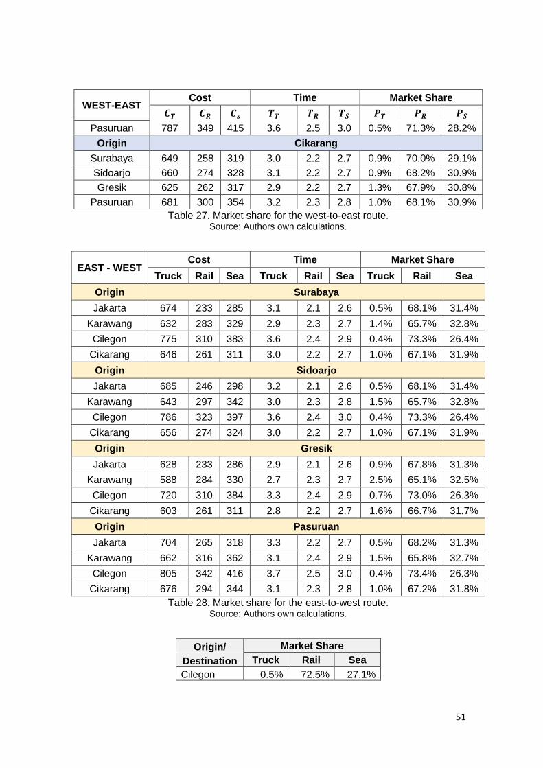
51

WEST-EAST Cost Time Market Share

𝑪𝑻 𝑪𝑹 𝑪𝒔 𝑻𝑻 𝑻𝑹 𝑻𝑺 𝑷𝑻 𝑷𝑹 𝑷𝑺

Pasuruan 787 349 415 3.6 2.5 3.0 0.5% 71.3% 28.2%

Origin Cikarang

Surabaya 649 258 319 3.0 2.2 2.7 0.9% 70.0% 29.1%

Sidoarjo 660 274 328 3.1 2.2 2.7 0.9% 68.2% 30.9%

Gresik 625 262 317 2.9 2.2 2.7 1.3% 67.9% 30.8%

Pasuruan 681 300 354 3.2 2.3 2.8 1.0% 68.1% 30.9%

Table 27. Market share for the west-to-east route. Source: Authors own calculations.

EAST - WEST Cost Time Market Share

Truck Rail Sea Truck Rail Sea Truck Rail Sea

Origin Surabaya

Jakarta 674 233 285 3.1 2.1 2.6 0.5% 68.1% 31.4%

Karawang 632 283 329 2.9 2.3 2.7 1.4% 65.7% 32.8%

Cilegon 775 310 383 3.6 2.4 2.9 0.4% 73.3% 26.4%

Cikarang 646 261 311 3.0 2.2 2.7 1.0% 67.1% 31.9%

Origin Sidoarjo

Jakarta 685 246 298 3.2 2.1 2.6 0.5% 68.1% 31.4%

Karawang 643 297 342 3.0 2.3 2.8 1.5% 65.7% 32.8%

Cilegon 786 323 397 3.6 2.4 3.0 0.4% 73.3% 26.4%

Cikarang 656 274 324 3.0 2.2 2.7 1.0% 67.1% 31.9%

Origin Gresik

Jakarta 628 233 286 2.9 2.1 2.6 0.9% 67.8% 31.3%

Karawang 588 284 330 2.7 2.3 2.7 2.5% 65.1% 32.5%

Cilegon 720 310 384 3.3 2.4 2.9 0.7% 73.0% 26.3%

Cikarang 603 261 311 2.8 2.2 2.7 1.6% 66.7% 31.7%

Origin Pasuruan

Jakarta 704 265 318 3.3 2.2 2.7 0.5% 68.2% 31.3%

Karawang 662 316 362 3.1 2.4 2.9 1.5% 65.8% 32.7%

Cilegon 805 342 416 3.7 2.5 3.0 0.4% 73.4% 26.3%

Cikarang 676 294 344 3.1 2.3 2.8 1.0% 67.2% 31.8%

Table 28. Market share for the east-to-west route. Source: Authors own calculations.

Origin/ Market Share

Destination Truck Rail Sea

Cilegon 0.5% 72.5% 27.1%

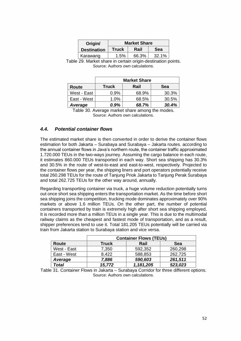
52

Origin/ Market Share

Destination Truck Rail Sea

Karawang 1.5% 66.3% 32.1%

Table 29. Market share in certain origin-destination points. Source: Authors own calculations.

Market Share

Route Truck Rail Sea

West - East 0.9% 68.9% 30.3%

East - West 1.0% 68.5% 30.5%

Average 0.9% 68.7% 30.4%

Table 30. Average market share among the modes. Source: Authors own calculations.

4.4. Potential container flows

The estimated market share is then converted in order to derive the container flows estimation for both Jakarta – Surabaya and Surabaya – Jakarta routes. according to the annual container flows in Java’s northern route, the container traffic approximated 1.720.000 TEUs in the two-ways journey. Assuming the cargo balance in each route, it estimates 860.000 TEUs transported in each way. Short sea shipping has 30.3% and 30.5% in the route of west-to-east and east-to-west, respectively. Projected to the container flows per year, the shipping liners and port operators potentially receive total 260.298 TEUs for the route of Tanjung Priok Jakarta to Tanjung Perak Surabaya and total 262.725 TEUs for the other way around, annually.

Regarding transporting container via truck, a huge volume reduction potentially turns out once short sea shipping enters the transportation market. As the time before short sea shipping joins the competition, trucking mode dominates approximately over 90% markets or above 1.6 million TEUs. On the other part, the number of potential containers transported by train is extremely high after short sea shipping employed, It is recorded more than a million TEUs in a single year. This is due to the multimodal railway claims as the cheapest and fastest mode of transportation, and as a result, shipper preferences tend to use it. Total 181.205 TEUs potentially will be carried via train from Jakarta station to Surabaya station and vice versa.

Container Flows (TEUs)

Route Truck Rail Sea

West - East 7,350 592,352 260,298

East - West 8,422 588,853 262,725

Average 7,886 590,603 261,511

Total 15,772 1,181,205 523,023

Table 31. Container Flows in Jakarta – Surabaya Corridor for three different options. Source: Authors own calculations.

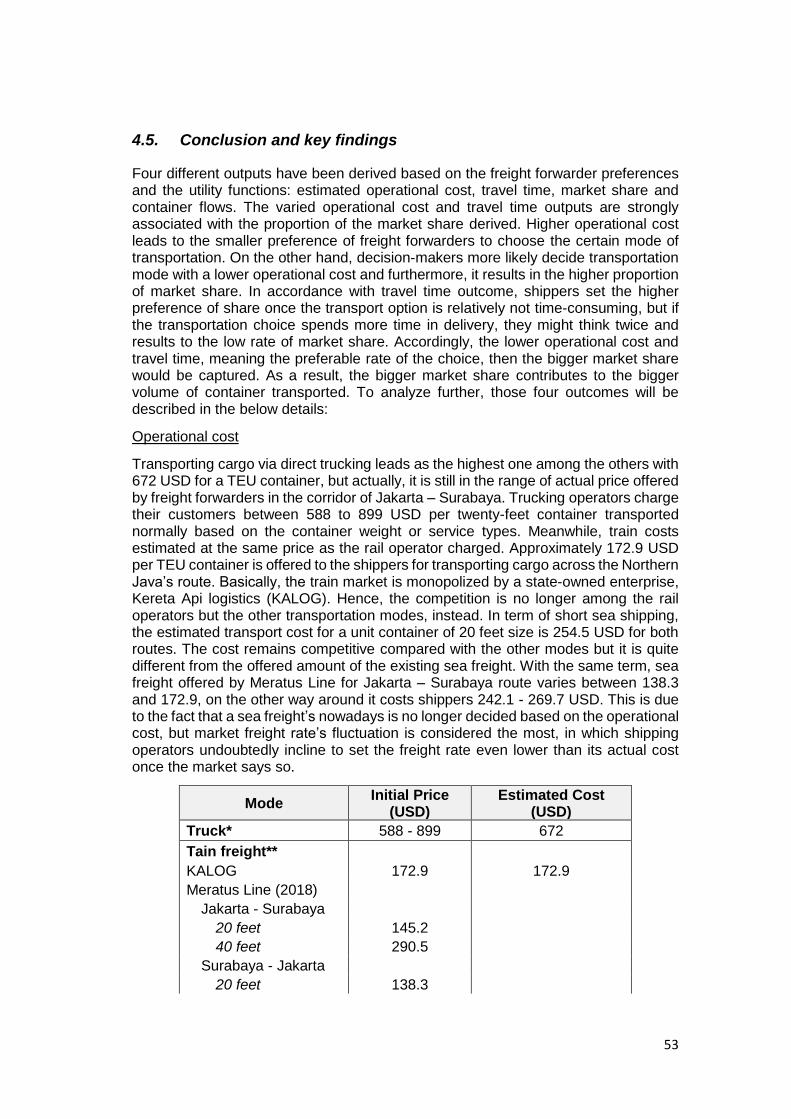
53

4.5. Conclusion and key findings

Four different outputs have been derived based on the freight forwarder preferences and the utility functions: estimated operational cost, travel time, market share and container flows. The varied operational cost and travel time outputs are strongly associated with the proportion of the market share derived. Higher operational cost leads to the smaller preference of freight forwarders to choose the certain mode of transportation. On the other hand, decision-makers more likely decide transportation mode with a lower operational cost and furthermore, it results in the higher proportion of market share. In accordance with travel time outcome, shippers set the higher preference of share once the transport option is relatively not time-consuming, but if the transportation choice spends more time in delivery, they might think twice and results to the low rate of market share. Accordingly, the lower operational cost and travel time, meaning the preferable rate of the choice, then the bigger market share would be captured. As a result, the bigger market share contributes to the bigger volume of container transported. To analyze further, those four outcomes will be described in the below details:

Operational cost

Transporting cargo via direct trucking leads as the highest one among the others with 672 USD for a TEU container, but actually, it is still in the range of actual price offered by freight forwarders in the corridor of Jakarta – Surabaya. Trucking operators charge their customers between 588 to 899 USD per twenty-feet container transported normally based on the container weight or service types. Meanwhile, train costs estimated at the same price as the rail operator charged. Approximately 172.9 USD per TEU container is offered to the shippers for transporting cargo across the Northern Java’s route. Basically, the train market is monopolized by a state-owned enterprise, Kereta Api logistics (KALOG). Hence, the competition is no longer among the rail operators but the other transportation modes, instead. In term of short sea shipping, the estimated transport cost for a unit container of 20 feet size is 254.5 USD for both routes. The cost remains competitive compared with the other modes but it is quite different from the offered amount of the existing sea freight. With the same term, sea freight offered by Meratus Line for Jakarta – Surabaya route varies between 138.3 and 172.9, on the other way around it costs shippers 242.1 - 269.7 USD. This is due to the fact that a sea freight’s nowadays is no longer decided based on the operational cost, but market freight rate’s fluctuation is considered the most, in which shipping operators undoubtedly incline to set the freight rate even lower than its actual cost once the market says so.

Mode Initial Price

(USD) Estimated Cost

(USD)

Truck* 588 - 899 672

Tain freight**

KALOG 172.9 172.9

Meratus Line (2018)

Jakarta - Surabaya

20 feet 145.2

40 feet 290.5

Surabaya - Jakarta

20 feet 138.3

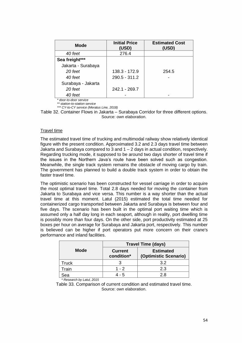
54

Mode Initial Price

(USD) Estimated Cost

(USD)

40 feet 276.4

Sea freight***

Jakarta - Surabaya

20 feet 138.3 - 172.9 254.5

40 feet 290.5 - 311.2 -

Surabaya - Jakarta

20 feet 242.1 - 269.7

40 feet - - * door-to-door service ** station-to-station service *** CY-to-CY service (Meratus Line, 2018)

Table 32. Container Flows in Jakarta – Surabaya Corridor for three different options. Source: own elaboration.

Travel time

The estimated travel time of trucking and multimodal railway show relatively identical figure with the present condition. Approximated 3.2 and 2.3 days travel time between Jakarta and Surabaya compared to 3 and 1 – 2 days in actual condition, respectively. Regarding trucking mode, it supposed to be around two days shorter of travel time if the issues in the Northern Java’s route have been solved such as congestion. Meanwhile, the single track system remains the obstacle of moving cargo by train. The government has planned to build a double track system in order to obtain the faster travel time.

The optimistic scenario has been constructed for vessel carriage in order to acquire the most optimal travel time. Total 2.8 days needed for moving the container from Jakarta to Surabaya and vice versa. This number is a way shorter than the actual travel time at this moment. Latul (2015) estimated the total time needed for containerized cargo transported between Jakarta and Surabaya is between four and five days. The scenario has been built in the optimal port waiting time which is assumed only a half day long in each seaport, although in reality, port dwelling time is possibly more than four days. On the other side, port productivity estimated at 25 boxes per hour on average for Surabaya and Jakarta port, respectively. This number is believed can be higher if port operators put more concern on their crane's performance and inland facilities.

Mode

Travel Time (days)

Current condition*

Estimated (Optimistic Scenario)

Truck 3 3.2

Train 1 - 2 2.3

Sea 4 - 5 2.8 * Research by Latul, 2015

Table 33. Comparison of current condition and estimated travel time. Source: own elaboration.

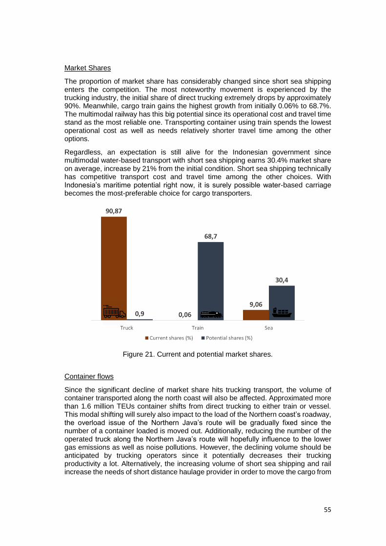
55

Market Shares

The proportion of market share has considerably changed since short sea shipping enters the competition. The most noteworthy movement is experienced by the trucking industry, the initial share of direct trucking extremely drops by approximately 90%. Meanwhile, cargo train gains the highest growth from initially 0.06% to 68.7%. The multimodal railway has this big potential since its operational cost and travel time stand as the most reliable one. Transporting container using train spends the lowest operational cost as well as needs relatively shorter travel time among the other options.

Regardless, an expectation is still alive for the Indonesian government since multimodal water-based transport with short sea shipping earns 30.4% market share on average, increase by 21% from the initial condition. Short sea shipping technically has competitive transport cost and travel time among the other choices. With Indonesia’s maritime potential right now, it is surely possible water-based carriage becomes the most-preferable choice for cargo transporters.

Figure 21. Current and potential market shares.

Container flows

Since the significant decline of market share hits trucking transport, the volume of container transported along the north coast will also be affected. Approximated more than 1.6 million TEUs container shifts from direct trucking to either train or vessel. This modal shifting will surely also impact to the load of the Northern coast’s roadway, the overload issue of the Northern Java’s route will be gradually fixed since the number of a container loaded is moved out. Additionally, reducing the number of the operated truck along the Northern Java’s route will hopefully influence to the lower gas emissions as well as noise pollutions. However, the declining volume should be anticipated by trucking operators since it potentially decreases their trucking productivity a lot. Alternatively, the increasing volume of short sea shipping and rail increase the needs of short distance haulage provider in order to move the cargo from

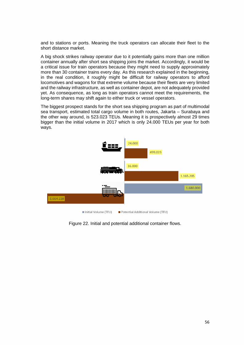
56

and to stations or ports. Meaning the truck operators can allocate their fleet to the short distance market.

A big shock strikes railway operator due to it potentially gains more than one million container annually after short sea shipping joins the market. Accordingly, it would be a critical issue for train operators because they might need to supply approximately more than 30 container trains every day. As this research explained in the beginning, in the real condition, it roughly might be difficult for railway operators to afford locomotives and wagons for that extreme volume because their fleets are very limited and the railway infrastructure, as well as container depot, are not adequately provided yet. As consequence, as long as train operators cannot meet the requirements, the long-term shares may shift again to either truck or vessel operators.

The biggest prospect stands for the short sea shipping program as part of multimodal sea transport, estimated total cargo volume in both routes, Jakarta – Surabaya and the other way around, is 523.023 TEUs. Meaning it is prospectively almost 29 times bigger than the initial volume in 2017 which is only 24.000 TEUs per year for both ways.

Figure 22. Initial and potential additional container flows.

57

Chapter 5 Conclusion Through the conditional logit model given the utility functions, this research aims to find out the potential market share and number of transported containers of water-based mode once it is involved in the market. This chapter briefly describes the answers of the research questions which already constructed in the first chapter as well as links the outcome values of the proposed transportation mode, short sea shipping, and the actual Indonesian maritime condition by giving some advises based on the qualitative analysis including what kind of possibilities can happen and how the government and the stakeholders should react. Moreover, research limitations and some suggestions which might be useful for the further research are also given as follows.

5.1. Answers to the research questions

As it is explained in the first chapter, this research has two sub-research questions which need to be answered before come to the central research question. The sub-research questions are re-described and answered as follows :

What is the estimated total cost for moving cargo using direct trucking, multimodal rail transport and multimodal short sea shipping across the northern Java’s Route?

Using a cost analysis method for each different modes, estimated total costs are derived in term of door-to-door service. Transporting container using direct trucking costs freight forwarders 672 USD on average, multimodal rail transport is 172.9 USD, and 254.5 USD for multimodal short sea shipping.

What is the estimated travel time for transporting cargo along the northern Java’s route for each different transportation mode (truck, multimodal rail transport, and multimodal sea transport)?

Travel time analysis is constructed to gain the delivery time for each transportation choice. It results in three different figures for each mode; trucking haulage spends approximately 3.2 days to transport a container along the route, meanwhile, multimodal rail transport promises 2.3 days, and lastly, using short sea shipping as part of multimodal sea transport, freight forwarder only spend 2.8 days to move a TEU container.

Using the results of sub-research questions, then we can briefly answer the main research question as concluded below:

How are the potential market share and transported container volume by the alternative transportation mode, Short sea shipping, in the northern Java’s route?

Potential market shares are calculated using conditional logit model given the utility

functions of cost and travel time attributes. Short sea shipping as part of multimodal

sea transport obtains a potential figure with 30.4% shares among the other choices.

Meanwhile, the estimated volume transported is 523.023 TEU containers annually

along Jakarta – Surabaya corridor.

5.2. Advice

Short sea shipping has excellent potential figures on the estimated market share by 30.4% or total 523.023 TEU containers in Jakarta – Surabaya corridor. The containers shifting is mostly derived from the trucking mode which might not be reliable enough

58

on the next following years. Regardless, this substantial increase should be anticipated by shipping companies, port or terminal operators, and the government in order to accommodate sufficient container flows.

In comparison with the other transport modes, despite the following issues that must be encountered by the maritime industry actors, the infrastructure of vessel transport seems to be the most-prepared one. In addition, the number of vessel units is relatively available and ready to deploy by the shipping companies who are interested to grab the Jakarta – Surabaya corridor’s market. On the other hand, the two biggest Indonesian seaports are eligible to deliver the service. Before going further to decide whether we should immediately move to the water-based carriage or not, some notes need to take into account for four different Indonesian maritime industry actors: port companies, shipping lines, freight forwarders, and the government.

It is obvious that the main obstacle for applying seagoing transport along the Northern Java’s coast nowadays is mostly on the port side, even though the two massive seaports are ready to serve Jakarta – Surabaya routes, but numerous home-works remain need to be done. Pelindo II and Pelindo III as a state-owned port company and operator in Jakarta and Surabaya, respectively, still have some operational issues such as low crane productivity, lack of berthing space availability, high port dwelling time, and insufficient inland facilities. However, the port is a key infrastructure and a starting point to re-develop Indonesian maritime sector, therefore, Pelindo II and Pelindo III on behalf of Indonesian port companies have a primary role to encourage the other maritime-based firms to build up the industry one more time. Once the port industry is constantly fixing the issues, we believe the other sectors will gradually follow.

The second industry that hopefully follows is shipping. There are various container shipping operators in Indonesia, and the few biggest companies namely Meratus Line, SPIL line, Tanto line, Temas Line and Samudera Indonesia. Whether or not, a huge support by shipping companies is certainly needed to start the service between Jakarta and Surabaya. It is probably a risky decision and it needs an accurate consideration for shipping firms to run the new market which is still not well-proven yet. That is the reason that stable and well-financed shipping companies are apparently required to collaborate with the port companies in order to assist the service.

Freight forwarding industry stands in the front position to connect with the shippers or cargo owners. Moreover, Freight forwarders have a vital role to drive the shipment market as well as considering which transportation mode is the most suitable to move their containers. Thus, shipping companies and the government should facilitate freight forwarders in order to drive their preferences to choose vessel as the main carriage.

Last but not least, the role of the local government is another key factor to re-develop the Indonesian maritime sector. The current Indonesian President, Joko Widodo, has full attention to the national maritime sector, proved by allocating national equities in several maritime-based stated owned enterprises, constructing maritime infrastructures, and launching various maritime-based programs. However, despite the year 2019 is the election year and the decision makers might change, this maritime path must remain to continue for the following regimes.

In conclusion, the potential share of short sea shipping is only a figure. That figure might be useful for Indonesian maritime industry or the government to be more

59

optimistic that they remain to have an expectation to awake their maritime potential, but there is something more important to consider. At the moment, the point is not when the implementation of short sea shipping should be started, but how we can reach that figure, the figure of 30.4% market share of the sea-based carriage, it is not easily granted as we employ the short sea shipping program tomorrow, it needs serious preparations and readiness. The readiness of all maritime sectors in Indonesia such as ports, shipping lines, and freight forwarders, the readiness to collaborate within the sectors, the readiness of improving the sector’s quality and the readiness of the government to sustainably support the maritime sectors.

5.3. Limitations of research and suggestions for further study

Some limitations have been applied in this research due to various reasons such as simplification, data availability, time restriction, and technological gap. These limitations hopefully can deliver an accurate interpretation of the research’s outputs to the reader as well as give the further outlook when the new studies intend to be performed.

This research focuses on the containerized cargo in 20 feet size in order to adapt to the vessel and port/terminal performances. Vessel’s data are mostly gained from the container vessel’s operators and also it is easier to derive container terminal performance data than breakbulk or the other terminals. In addition, TEU container unit is broadly applicable for every different transportation modes, therefore, trucking, railway, and vessel operator are commonly familiar to handle containerized cargo. However, twenty-feet size container is decided since the majority of container transported in Indonesia is dominated by this certain dimension, up to 80%. Meaning the division of container size, in which including 40 feet size, probably will not significantly impact to the cost variable.

Various terms of service are normally provided by the freight forwarder to determine the freight rate, namely, door-to-door, door-to-port, port-to-port, port-to-CY, station-to-station and many more. In this case, we only put the door-to-door term into the calculation scenario in order to simplify the measurement as well as to make it is universally accepted in which every transportation modes are familiar using it. It is suggested to the further studies to initially observe which term considered as the most-employed service given by freight forwarders for each mode. The preferences of every modal choice might be various since it produces different operational costs and service.

Stated preference analysis is supposed to be directly employed in order to gain the coefficient of utility functions in the current situation. Freight forwarder preferences are a way better to derive from the actual circumstances where the study taking place in order to know the local preferences instead of taking from another study in which have different study case location. Because of time limitation and technological issue for Indonesian freight forwarders in which makes us difficult to contact, the coefficients of utility function were borrowed from another study which has similar conditions and circumstances. Consequently, the attributes used are only operational cost and travel time due to it is adjusted from the study that also brings merely cost and time coefficients. To develop advanced accuracy of the results, the attributes can be added more details such as schedule frequency, carrying capacity, reliability, safety and etc.

Railway cost calculation becomes an attention point since it was only derived from rail freight of local operators due to it is quite complicated to break down the cost structure

60

as well as insufficient data availability. On the other hand, limitation of cost and time analysis for vessel transport is described separately in details by Sudjaka (2018) in the different study as part of the joint thesis project.

Despite the central development and concentrated cargo flows, Indonesia is not merely Java island. The primary objective of the Indonesian government nowadays is removing economics gap among the other regions, especially Java and the other islands. As a maritime country, short sea shipping is hopefully can be applied in every maritime-based regions in Indonesia in order to solve the national issues. The following research expectantly can reveal the potential of water-based transportation’s utilization in the other regions of Indonesia.

61

References

Bahagia, S N, Sandee, H. & Meeuws, R (2015). ‘State of Logistics Indonesia 2015’. Jakarta: State Secretariat for Economic Affairs SECO Switzerland.

Balduini, G (1982). ‘Italy’. Short-sea Shipping in the Economy of Inland Transport in Europe: A Report of the Sixtieth Round Table on Transport Economics Held in Gothenburg, Sweden. OECD Publications and Information Centre. Washington, DC (April 1–2), pp. 37–65.

Bagchus, R C, Kuipers, B (1993). ‘Autrostrada del mare’. Windjnolst, Ir.N., Peeters, C., Liebman, P. (Eds.), European Shortsea Shipping, Proceedings from the First European Roundtable Conference on Shortsea Shipping. LLP, London, pp. 52–65.

Beni-Akiva, M, and Lermani S R (1985). Discrete Choice Analysis. Cambridge Mass : MllT Press.

Bergantino, A and Bolis, S (2004). ‘Ananalysis of maritime ro–ro freight transport service attributes through adaptive stated preference: an application to a sample of freight forwarders’. European Transport, pp 25–26, 33–51.

Bjornland, D (1993). ‘The importance of Short Sea Shipping in European Transport’. ECMT: Short Sea Shipping. OECD, Paris, pp. 59–93.

Blonk, W (1993). ‘Policy Recommendations’. Windjnolst, Ir.N., Peeters, C., Liebman, P. (Eds.), European Shortsea Shipping, Proceedings from the First European Roundtable Conference on Shortsea Shipping. LLP, London.

Boediono, L (2018). ‘Indonesia Continues to Build on Solid Economic Growth’. Retrieved July 21, 2018, from http://www.worldbank.org/en/news/press-release/2018/03/27/indonesia-continues-to-build-on-solid-economic-growth

Brooks M R and Frost, J D (2004). ‘Short sea shipping: a Canadian perspective’. Maritime Policy & Management, vol. 31(4), 393-407, DOI: 10.1080/0308883042000304881.

Commission of the European Communities (1992). Council Regulation (EEC) No. 3577/1992, Applying the Principle of Freedom to Provide Services to Maritime Transport Within Member States (maritime cabotage). Brussels, O J no. L 364.

COM (2003). The programme for the promotion of Short Sea Shipping. (Communication from the European Commission). Brussels: 8 april. 155 final.

COM (2011). White Paper. Roadmap to a Single European Transport Area – Towards a competitive and resource efficient transport system. European Commission.

Crainic, T G and Kap, H K (2007). ‘Intermodal Transportation’. Handbook in Operation Research & Management Science, Elsevier, vol. 14 Chapter 8. https://doi.org/10.1016/S0927-0507(06)14008-6UR

Criley, J and Dean, C J (1993). ‘Shortsea shipping and the world cargo-carrying fleet – a statistical summary’. Windjnolst, Ir.N., Peeters, C., Liebman, P. (Eds.), European Shortsea Shipping, Proceedings from the First European Roundtable Conference on Shortsea Shipping. LLP, London, pp. 1–21.

62

European Commission (2001). European Transport Policy for 2010: Time to Decide. Luxembourg: European Commission.

Eurostat (2006). European Union Transport in Figures. Statistical Pocket Book, Office for Official Publications of the European Communities, Luxembourg.

GAO (2005). Freight Transportation: Short Sea Shipping Option Shows Importance of Systematic Approach to Public Investment Decisions. Washington, DC, http://www.gao.gov/newitems/d05768pdf

Gattuso, D. and Restuccia, A (2014). ‘A Tool for Railway Transport Cost Evaluation’. Procedia - Social and Behavioral Sciences, vol. 111, pp: 549-558, ISSN 1877-0428. Elsevier Science Ltd.

Henesey, L and Yonge, M (2006). Short Sea Shipping in the United States: Identifying the Prospects and Opportunities. TRB 85th Annual Meeting 2006, Compendium of Papers CD-ROM, pp. 16–32.

Hoffman, S D, and Duncan, G J (1988). ‘Multinomial and Conditional Logit Discrete-Choice Models in Demography’. Springer: Demography, vol. 25, No. 3 (Aug., 1988), pp. 415-427

Hoogerbeets, J and Melissen, P (1993). ‘Facilitation of shortsea shipping: Improvements in the sea/land interface (the dutch case)’. Windjnolst, Ir.N., Peeters, C., Liebman, P. (Eds.), European Shortsea Shipping, Proceedings from the First European Roundtable Conference on Shortsea Shipping. LLP, London, pp. 346–350.

KALOG (2018). KALOG - Produk & Layanan > Ka_angkutan_container. Retrieved July 23, 2018, from http://www.kalogistics.co.id/layanan_product/ka_angkutan_container#.W1Xz2tIzbIU

Koppelman, F S, and Bhat, S (2006). ‘A Self Instructing Course in Mode Choice Modeling: Multinomial and Nested Logit Models. U.S.’. Journal of Department of Transportation - Federal Transit Administration.

Latul, J (2015). ‘Indonesia Shipping: Riding the wave with Capt. Jokowi’. CLSA: Sector Outlook.

Lombardo, G A (2004). ‘Short Sea Shipping: Practices, Opportunities and Challenges’. Transportgistics.

MB Logistics (2018). Tariff and Sector for Jakarta and Surabaya Area. Surabaya

McFadden, D (1974). ‘The measurement of urban travel demand’. Journal of Public Economics, vol. 3, pp.303–328.

Medda, F and Trujillo, L (2010). ‘Short-sea shipping: an analysis of its determinants’. Maritime Policy & Management, vol. 37:3, 285-303, DOI: 10.1080/03088831003700678

Meyer, J, Stahlbock, R, and Voss, S (2012). ‘Slow Steaming in Container Shipping’. International Conference on System Sciences. 1306-1314. 10.1109/HICSS.2012.529.

Ministry of Transportation (2013). Studi Jaringan Prasarana dan Pelayanan Kereta Api Barang Dalam Mengurangi Beban Jalan. Jakarta

63

Musso, E and Marchese, U (2002). ‘Economics of short sea shipping’. T.H. Costas Grammenos (ed.) The Hanbook of Maritime Economics and Business. LLP: Informa professional.

Nash, C. (2000). Modelling Performance: Rail. D.A. Hensher, & K. J. Button (Eds.), Handbook of Transport Modelling, pp. 565-575. Elsevier Science Ltd.

Ortuzar, J D, and Willumsen, L G (1990). Modelling Transport. England : John Wiley & Sons

Paixão, A C and Marlow, P B (2002). ‘Strengths and weaknesses of short sea shipping’. Marine Policy, Elsevier, vol. 26(3), pages 167-178, May.

Paixão, A C and Marlow, P B (2004). ‘Short sea shipping and its role in logistics supply chains: A European perspective’. Journal of International Logistics and Trade, vol. 2(1): 57–68.

Patterson, Z, Ewing, G and Haider, M (2004). ‘Shipper preferences suggest strong mistrust of rail’. Transportation Research Record, vol. 1, 67–74.

Peeters, C M (1993). ‘Key-note address’. Windjnolst, Ir.N., Peeters, C., Liebman, P. (Eds.), European Shortsea Shipping, Proceeding from the First European Roundtable Conference on Shortsea Shipping. LLP, London.

Perakis, A. and Denisis, A (2008). ‘A survey of short sea shipping and its prospects in the USA’. Maritime Policy and Management. Vol. 35(6): 591–614.

Psaraftis, H N, and Papanikolaou, A D (1993). ‘Impact of new technologies on shortsea shipping in Greece’. Windjnolst, Ir.N., Peeters, C., Liebman, P. (Eds.), European Shortsea Shipping, Proceedings from the First European Roundtable Conference on Shortsea Shipping. LLP, London, pp. 79–94.

Psaraftis, H N and Schinas, O D (1996). .Concerted Action on Short Sea Shipping’. : State of the Art, vol. 2, Part I, July 8.

Realise (2002). Regional Action for Logistical Integration of Shipping across Europe. The Alliance of Maritime Regional Interests in Europe (AMRIE), GTC2-2000-33032.

Ricci, A. and Black, I (2005). ‘The social cost of intermodal freight transport’. Measuring the Marginal Social Cost of Transport. Research in Transportation Economics. edited by C. Nash and B. Matthews, vol. 14 (UK: Elsevier), pp. 245–285.

SCOOP (2004). ‘The Public Benefits of The Short-Sea Intermodal System’. The Short Sea Cooperative Program (SCOOP). University of New Orleans: National Ports and Waterways Institute.

Smith, A (1998). An Inquiry into the Nature and Causes of the Wealth of Nations. Oxford: Oxford University Press.

Stopford, M (1997). Maritime Economics. Routledge, London.

Stramindo (2003). Final report summary : Study on the Development of Domestic Sea Transportation and Maritime Industry in the Republic of Indonesia.

Suárez-Alemán, A, Campos, J, and Jimenez, J L (2014). ‘The economic competitiveness of short sea shipping: An empirical assessment for Spanish ports’. International Journal of Shipping and Transport Logistics. Forthcoming.

64

Suarez-Alleman, A, Trujillo, L, Cullinane, K P B (2014). ‘Time at ports in short sea shipping: When timing is crucial’. Maritime Economics & Logistics. Volume 16, Issue 4, pp 399–417. https://doi.org/10.1057/mel.2014.5DO

Supply Chain Indonesia (2016a). ‘Kumpulan Data Pelabuhan Laut Indonesia’. Pusat Data Logistik: Supply Chain Indonesia.

Supply Chain Indonesia (2016b). ‘Kumpulan Data Transportasi Barang Indonesia’. Pusat Data Logistik: Supply Chain Indonesia.

UNITE (2002). Mediterranean Short-Sea Shipping including Piraeus Port Marginal Cost Case Study. Version 1.1, D.Tsamboulas, D. Korizis, A. Kopsacheili, SYSTEMA.

UNITE (2003). Final Report, version 1.0. C. Nash, ITS, University of Leeds, UK.

US Department of Transportation (2008). Maritime Administration. Short Sea Shipping Brochure.

Van Gunsteren, L A, Van Popta, T, Ravenhorst, R E G (1993). ‘Is continental and intercontinental cargo waiting for shortsea shipping?’. Windjnolst, Ir.N., Peeters, C., Liebman, P. (Eds.), European Shortsea Shipping, Proceedings from the First European Roundtable Conference on Shortsea Shipping. LLP, pp. 245–255.

Van Willigenburg, J R, Hollander, S (1993). ‘Coastal shipping oportunities in a changing market’. Windjnolst, Ir.N., Peeters, C., Liebman, P. (Eds.), European Shortsea Shipping, Proceedings from the First European Roundtable Conference on Shortsea Shipping. LLP, pp. 184–192.

Veldman, S. and Bossche, v d M (2012). ‘Assessing a short-sea liner shipping potential: example of Portuguese short-sea trades’. International Research Conference on Short Sea Shipping (2012: Lisbon, Portugal).

Veldman, S, Garcia-Alonso, L, and Vallejo-Pinto, J A (2013). ‘A port choice model with logit models: a case study for the Spanish container trades’. International Journal of Shipping and Transport Logistics, vol. 5, Nos. 4/5, 2013.

Veldman, S (1994). ‘Aspects of Port Choice with Container Shipping, an example with Polish container ports’. Roundtable Conference of Gdansk University (1994: Sopot, Poland).

Veldman, S (2011). On the ongoing increase of containership size. Chapter in Advances in Maritime Logistics and Supply Chain Systems, World Scientific Publishing Company Pte, Ltd, Singapore

Wang, S and Meng, Q (2012). ‘Sailing speed optimization for container ships in a liner shipping network’. Transportation Research Part E, vol. 48, 701–714. https://doi.org/10.1016/j.tre.2011.12.003

Wismadi, A J, Soemardjito and Sutomo H (2013), ‘Transport Situation in Jakarta’, in Kutani, I. (ed.), Study on energy efficiency improvement in the transport sector through transport improvement and smart community development in the urban area, ERIA Research Project Report 2012-29, pp.29-58. Available at: http:/www.eria.org/RPR_FY2012_No.29_Chapter_4.pdf

Whitelegg, J (1997). ‘Evaluating strategic trans-shipment sites and urban distribution centres’. Sustainable Freight Transport in the City, Conference Papers, September 24–25, Transport 2000, London.

65

World Shipping Council - Partners in Trade. Retrieved July 22, 2018, from http://www.worldshipping.org/about-the-industry/global-trade/top-50-world-container-ports