Embed Size (px)
Citation preview
Available online at www.sciencedirect.com
Journal of Functional Analysis 261 (2011) 3696–3722
www.elsevier.com/locate/jfa
Equivalence of K- and J -methods for limiting realinterpolation spaces
Fernando Cobos a,∗,1, Thomas Kühn b,1
a Departamento de Análisis Matemático, Facultad de Matemáticas, Universidad Complutense de Madrid,Plaza de Ciencias 3, 28040 Madrid, Spain
b Mathematisches Institut, Fakultät für Mathematik und Informatik, Universität Leipzig, Johannisgasse 26,D-04103 Leipzig, Germany
Received 29 July 2010; accepted 31 August 2011
Available online 13 September 2011
Communicated by Alain Connes
Abstract
We consider limiting real interpolation spaces defined by using powers of iterated logarithms and showtheir description by means of the J -functional. Our results allow to complement some estimates on approx-imation of stochastic integrals.© 2011 Elsevier Inc. All rights reserved.
Keywords: Limiting interpolation spaces; J -functional; K-functional; Lorentz–Zygmund spaces; Besov spaces
1. Introduction
The real interpolation method (A0,A1)θ,q plays an outstanding role in applications of interpo-lation theory to functional analysis, harmonic analysis, approximation theory, partial differentialequations and some other domains of mathematics. We refer, for example, to the books by Butzerand Berens [7], Bergh and Löfström [5], Triebel [29], Bennett and Sharpley [4], Brudnyı andKrugljak [6], Connes [12] and Amrein, Boutet de Monvel and Georgescu [2].
The most familiar definitions of (A0,A1)θ,q are those given by Peetre’s K- and J -functional.The equivalence theorem (see [5, Section 3.3]) shows that these constructions produce the same
* Corresponding author.E-mail addresses: [email protected] (F. Cobos), [email protected] (T. Kühn).
1 Authors have been supported in part by the Spanish Ministerio de Ciencia e Innovación (MTM2010-15814).
0022-1236/$ – see front matter © 2011 Elsevier Inc. All rights reserved.doi:10.1016/j.jfa.2011.08.018
F. Cobos, T. Kühn / Journal of Functional Analysis 261 (2011) 3696–3722 3697
space. This fact is an important item in the development of the theory. In fact, it yields densityof A0 ∩ A1 in (A0,A1)θ,q if q < ∞, and it is useful to establish the reiteration theorem or theduality theorem, among other results.
The definition of (A0,A1)θ,q requires 0 < θ < 1, but certain questions in function spaces havemotivated the investigation of limiting real interpolation spaces. Then θ = 0 or θ = 1, and thedefinition may also include logarithmic terms. See, for example, the book by Milman [25] andthe papers by Gomez and Milman [22], Doktorskii [13], Evans and Opic [15], Evans, Opic andPick [16], Gogatishvili, Opic and Trebels [21], Cobos, Fernández-Cabrera, Kühn and Ullrich [9],Cobos, Fernández-Cabrera and Mastyło [10], Fernández-Martínez and Signes [17] and Ahmed,Edmunds, Evans and Karadzhov [1].
Working with limiting methods, it is natural to restrict to ordered couples, where A0 ↪→ A1.If θ = 0 these methods produce spaces which are very close to A0, and when θ = 1 they are verynear to A1.
Among the limiting methods, K-methods have been more widely used than J -methods.Equivalence between limiting K- and J -constructions is only known for some choices of pa-rameters and, on the contrary to the case of the real method, an adjustment is needed with theeffect that a logarithmic factor should be inserted to obtain the K-description of a limiting J -space (see [9, Theorem 4.2] and [10, Corollary 5.10]).
In September 2009, Stefan Geiss [18] asked one of the present authors about the J -descriptionof the K-spaces defined by the condition
supt�e
K(t, a)
(log t)α< ∞. (1.1)
Here α > 0 is arbitrary. The motivation for this question is the potential use of a limiting equiv-alence theorem in stochastic finance, more specifically, in approximation of stochastic integrals(see [19,20]).
K-spaces defined by (1.1) have been considered in [15,16,21,17]. Even more general K-spaces have been studied in these references, including in the definition powers of iteratedlogarithms and not only the L∞-norm but also the Lq -norm. However, their J -description hasnot been investigated yet, except for the case α = 1 in (1.1) (see [9]). Accordingly, in this paperwe establish J -descriptions for all these K-spaces. Our results reveal a new phenomenon relatedto the factor of correction: it changes with logarithms which define the K-spaces.
The paper is organized as follows. In Section 2 we fix notation and introduce the K- andJ -spaces that we are dealing with. Section 3 contains some basic properties of limiting spacesas well as some examples. The main results of the paper are in Section 4 where we prove theequivalence theorem. Our arguments are based on a modified version of the so-called funda-mental lemma of interpolation theory and do not use “divisibility results” or strong forms of thefundamental lemma. Finally, in Section 5, we establish limiting formulae for couples of vector-valued sequence spaces and we show that our results can be used to complement some estimatesof C. Geiss, S. Geiss and M. Hujo [19,20] on approximation of stochastic integrals using deter-ministic equidistant nets.
2. Preliminaries
For iterated logarithms we use the notation
L0(t) = t, L1(t) = log t and Lj (t) = log(Lj−1(t)
)if j > 1.
3698 F. Cobos, T. Kühn / Journal of Functional Analysis 261 (2011) 3696–3722
Similarly, we write
LL1(t) = 1 + log t and LLj (t) = 1 + log(LLj−1(t)
)if j > 1.
For iterated exponential functions we put
E0(t) = t, E1(t) = et and Ej (t) = eEj−1(t) if j > 1.
If α = (α0, α1, . . . , αm) ∈ Rm+1, we set
ϕα(t) =m∏
j=0
Lj (t)αj .
As usual, given any 1 � q � ∞, the conjugate index q ′ is defined by 1/q + 1/q ′ = 1, where weput 1/∞ = 0.
If X,Y are quantities depending on certain parameters, by X � Y we mean that there is aconstant c > 0 independent of all parameters such that X � cY . We put X ∼ Y if X � Y andY � X. Similarly, given two non-negative functions f (t), g(t) defined on G ⊆ R, we say thatthey are equivalent and we write f ∼ g if there are constants c1, c2 > 0 such that
c1f (t) � g(t) � c2f (t) for all t ∈ G.
Let A0,A1 be Banach spaces with A0 ↪→ A1. Here the symbol ↪→ means continuous embed-ding. For t > 0, Peetre’s K- and J -functionals are defined by
K(t, a) = K(t, a;A0,A1)
= inf{‖a0‖A0 + t‖a1‖A1 : a = a0 + a1, aj ∈ Aj
}, a ∈ A1,
and
J (t, a) = J (t, a;A0,A1) = max{‖a‖A0, t‖a‖A1
}, a ∈ A0.
Definition 2.1. Let A0,A1 be Banach spaces with A0 ↪→ A1. Suppose that 1 � q � ∞, m ∈N ∪ {0} and let α = (α0, α1, . . . , αm) ∈ R
m+1 such that the function ϕα satisfies⎧⎪⎪⎪⎪⎪⎨⎪⎪⎪⎪⎪⎩
( ∞∫Em(1)
1
ϕα(t)q
dt
t
)1/q
< ∞ if 1 � q < ∞,
supt�Em(1)
1
ϕα(t)< ∞ if q = ∞.
(2.1)
The K-space (A0,A1)α,q;K consists of all a ∈ A1 which have a finite norm
‖a‖α,q;K =
⎧⎪⎪⎪⎪⎪⎨⎪⎪⎪⎪⎪⎩
( ∞∫Em(1)
(K(t, a)
ϕα(t)
)qdt
t
)1/q
if 1 � q < ∞,
supt�Em(1)
K(t, a)
ϕα(t)if q = ∞.
F. Cobos, T. Kühn / Journal of Functional Analysis 261 (2011) 3696–3722 3699
The spaces described in Definition 2.1 are special cases of the general K-method studied in[6] and [27]. For a ∈ A1, it follows from
‖a‖A1 � K(1, a) � K(t, a), t � Em(1)
that
( ∞∫Em(1)
(1
ϕα(t)
)qdt
t
)1/q
‖a‖A1 � ‖a‖α,q;K. (2.2)
So (A0,A1)α,q;K = {0} if (2.1) does not hold.By (2.2), we have that (A0,A1)α,q;K ↪→ A1. Moreover, using that
K(t, a) � ‖a‖A0 if a ∈ A0,
it is easily checked that A0 ↪→ (A0,A1)α,q;K.
Example 2.2. If α0 > 0, or α0 = 0 and α1 > 1/q then ϕα satisfies (2.1). Condition (2.1) alsoholds if α0 = 0, α1 = · · · = αr−1 = 1/q and αr > 1/q for some 2 � r � m.
Example 2.3. If α0 > 1 then we have (A0,A1)α,q;K = A1 because
‖a‖α,q;K �( ∞∫Em(1)
(t‖a‖A1
ϕα(t)
)qdt
t
)1/q
� c‖a‖A1 .
Example 2.4. When m = 0 and α = (θ) with 0 < θ < 1, we recover the classical real interpo-lation space (A0,A1)θ,q realized as a K-space (see [5,29,4]). The case m ∈ N and α ∈ R
m+1
with 0 < α0 < 1 is a special case of the well-known real method with function parameter(see [23,24,28]). For this reason, we are only interested here in the case α0 = 0.
See [16,21,17] for other results on spaces (A0,A1)α,q;K . Next we introduce J -spaces.
Definition 2.5. Let A0,A1 be Banach spaces with A0 ↪→ A1. Suppose that 1 � q � ∞, m ∈N ∪ {0} and let β = (β0, β1, . . . , βm) ∈ R
m+1 such that the function ϕβ satisfies
⎧⎪⎪⎪⎪⎪⎨⎪⎪⎪⎪⎪⎩
( ∞∫Em(1)
(ϕβ(t)
t
)q ′dt
t
)1/q ′
< ∞ if 1 < q � ∞,
supt�Em(1)
ϕβ(t)
t< ∞ if q = 1.
(2.3)
3700 F. Cobos, T. Kühn / Journal of Functional Analysis 261 (2011) 3696–3722
The space (A0,A1)β,q;J is formed by all those a ∈ A1 for which there is a strongly measurablefunction u(t) with values in A0 such that
a =∞∫
Em(1)
u(t)dt
t(convergence in A1) (2.4)
and
( ∞∫Em(1)
(J (t, u(t))
ϕβ(t)
)qdt
t
)1/q
< ∞ (2.5)
(the integral should be replaced by the supremum if q = ∞). The norm in (A0,A1)β,q;J is
‖a‖β,q;J = inf
{( ∞∫Em(1)
(J (t, u(t))
ϕβ(t)
)qdt
t
)1/q}
where the infimum is taken over all representations u satisfying (2.4) and (2.5).
The spaces (A0,A1)β,q;J are particular cases of the general J -method (see [6,27]). Theyare also sitting between A0 and A1. Indeed, since any a ∈ A0 can be represented as a =∫ eEm(1)
Em(1)a dt/t , embedding A0 ↪→ (A0,A1)β,q;J follows by using that ϕβ is a continuous
function. On the other hand, given any a ∈ (A0,A1)β,q;J and any J -representation a =∫ ∞Em(1)
u(t) dt/t , we derive
‖a‖A1 �∞∫
Em(1)
∥∥u(t)∥∥
A1
dt
t
�( ∞∫Em(1)
(ϕβ(t)
t
)q ′dt
t
)1/q ′( ∞∫Em(1)
(J (t, u(t))
ϕβ(t)
)qdt
t
)1/q
.
By (2.3), the first integral in the last inequality is finite, so (A0,A1)β,q;J ↪→ A1.Note also that if (2.3) does not hold then ‖a‖β,q;J = 0 for any a ∈ A0. This fact can be shown
by following the same idea as in [7, Proposition 3.2.7]. Indeed, take any a ∈ A0 and let ψ(t) bea non-negative function satisfying that (
∫ ∞Em(1)
(ψ(t)/ϕβ(t))q dtt)1/q = 1. Put
u(t) = ψ(t)/t∫ ∞Em(1)
ψ(s)s
dss
a.
Then a = ∫ ∞u(t) dt . Using that J (t, u(t)) � t‖u(t)‖A for t � Em(1), we obtain
Em(1) t 0
F. Cobos, T. Kühn / Journal of Functional Analysis 261 (2011) 3696–3722 3701
( ∞∫Em(1)
ψ(s)
ϕβ(s)
ϕβ(s)
s
ds
s
)‖a‖β,q;J =
( ∞∫Em(1)
ψ(s)
s
ds
s
)‖a‖β,q;J
�( ∞∫Em(1)
ψ(s)
s
ds
s
)( ∞∫Em(1)
(J (t, u(t))
ϕβ(t)
)qdt
t
)1/q
�( ∞∫Em(1)
(ψ(t)
ϕβ(t)
)qdt
t
)1/q
‖a‖A0 = ‖a‖A0 .
Taking the supremum over all possible functions ψ we derive that
( ∞∫Em(1)
(ϕβ(s)
s
)q ′ds
s
)1/q ′
‖a‖β,q;J � ‖a‖A0 .
This yields that ‖a‖β,q;J = 0 if (2.3) is not satisfied.
Example 2.6. Condition (2.3) is satisfied if β0 < 1, or β0 = 1 and β1 < −1/q ′, or β0 = 1,β1 = · · · = βr−1 = −1/q ′ and βr < −1/q ′ for some 2 � r � m.
Example 2.7. When m = 0 and β = (θ) with 0 < θ < 1, we get again the real interpolation space(A0,A1)θ,q but this time in the form of a J -space (see [5,29]). When m ∈ N and β ∈ R
m+1 with0 < β0 < 1 we recover spaces described by the real method with function parameter (see [23,24]).If m = 0 = β0, we obtain spaces studied in [9] and [10].
3. Some properties and examples of limiting K-spaces
Let B = (B0,B1) be another couple of Banach spaces with B0 ↪→ B1. By T ∈ L(A, B) wemean that T is a bounded linear operator from A1 into B1, whose restriction to A0 gives abounded linear operator from A0 into B0. We put ‖T ‖Ai,Bi
for the norm of T acting from Ai
into Bi (i = 0,1). It is easy to check that the restriction
T : (A0,A1)α,q;K → (B0,B1)α,q;K
is also bounded. Next we estimate its norm in the limit case α0 = 0. We shall need the func-tions LLj . Given any real number α, we put α+ = max{α,0}.
Theorem 3.1. Let A = (A0,A1), B = (B0,B1) be couples of Banach spaces with A0 ↪→ A1,B0 ↪→ B1. Suppose that 1 � q � ∞,m ∈ N ∪ {0} and let α = (α0, α1, . . . , αm) ∈ R
m+1 such thatα0 = 0 and α1 > 1/q , or α0 = 0, α1 = · · · = αr−1 = 1/q and αr > 1/q for some 2 � r � m. IfT ∈ L(A, B) and Mi = ‖T ‖Ai,Bi
for i = 0,1, we have
‖T ‖(A0,A1)α,q;K,(B0,B1)α,q;K �{
M0 if M1 � M0,
M0∏m
j=1 LLα+
j
j (M1/M0) if M0 � M1.
3702 F. Cobos, T. Kühn / Journal of Functional Analysis 261 (2011) 3696–3722
Proof. Since
K(t, T a;B0,B1) � M0K(tM1/M0, a;A0,A1), t > 0, a ∈ A1,
and K(t, a) is an increasing function of t , for M1 � M0 we obtain
‖T a‖α,q;K � M0
( ∞∫Em(1)
(K(tM1/M0, a)
ϕα(t)
)qdt
t
)1/q
� M0‖a0‖α,q;K.
Suppose now M0 � M1. It follows by induction that
Lk(tM1/M0) � Lk(t)LLk(M1/M0), t � Ek(1), k ∈ N. (3.1)
We obtain
‖T a‖α,q;K � M0
( ∞∫Em(1)
(K(tM1/M0, a)
ϕα(tM1/M0)
ϕα(tM1/M0)
ϕα(t)
)qdt
t
)1/q
� M0 supt�Em(1)
{ϕα(tM1/M0)
ϕα(t)
}‖a‖α,q;K
� M0
m∏j=1
LLα+
j
j (M1/M0)‖a‖α,q;K,
where we have used (3.1) in the last inequality.The case q = ∞ can be treated analogously. �In the special case m = 1, α0 = 0 and α1 = 1, we recover a norm estimate established in [9,
Theorem 4.9].Next we give examples of limiting interpolation spaces. Let (Ω,μ) be a σ -finite measure
space and let w(x) be a weight on Ω , that is, a positive measurable function on Ω . As usual, weput
Lq(w) = {f : ‖f ‖Lq(w) = ‖wf ‖Lq < ∞}
.
Let w0,w1 be weights on Ω such that w0(x) � w1(x) μ-a.e. Then Lq(w0) ↪→ Lq(w1). Replac-ing w1(x) by w1(x)/Em(1), which only produces an equivalent norm in Lq(w1), we may assumethat Em(1)w1(x) � w0(x) μ-a.e. in Ω .
Theorem 3.2. Let (Ω,μ) be a σ -finite measure space, let 1 � q � ∞, m ∈ N ∪ {0} and letα = (α0, α1, . . . , αm) ∈ R
m+1 such that α0 = 0 and
⎧⎨⎩
α1 > 1/q (in this case we let r = 1),
or
α1 = · · · = αr−1 = 1/q and αr > 1/q for some 2 � r � m.
F. Cobos, T. Kühn / Journal of Functional Analysis 261 (2011) 3696–3722 3703
Let w0 and w1 be weights on Ω such that Em(1)w1(x) � w0(x) μ-a.e. Put
w(x) = w0(x)L1/qr
(w0(x)
w1(x)
)/ m∏j=r
Lαj
j
(w0(x)
w1(x)
).
Then we have with equivalent norms
(Lq(w0),Lq(w1)
)α,q;K = Lq(w).
Proof. Since
K(t, f ;Lq(w0),Lq(w1)
) ∼( ∫
Ω
[min
{w0(x), tw1(x)
}∣∣f (x)∣∣]q dμ(x)
)1/q
,
we obtain
‖f ‖α,q;K ∼( ∫
Ω
∣∣f (x)∣∣q ∞∫Em(1)
[min{w0(x), tw1(x)}
ϕα(t)
]qdt
tdμ(x)
)1/q
.
Let I be the interior integral. We have
I = w1(x)q
w0(x)/w1(x)∫Em(1)
(t
ϕα(t)
)qdt
t+ w0(x)q
∞∫w0(x)/w1(x)
(1
ϕα(t)
)qdt
t= I1 + I2.
To estimate I2, note that
(1
ϕα(t)
)q
=[(
m∏j=r
Lαj
j (t)
)q r−1∏j=1
Lj (t)
]−1
.
We let∏r−1
j=1 Lj (t) = 1 if r = 1. Take any ε > 0 such that (αr − ε) > 1/q. Using that
Lεr (t)
m∏j=r+1
Lαj
j (t) is equivalent to a non-decreasing function
and
L−εr (t)
m∏j=r+1
Lαj
j (t) is equivalent to a non-increasing function
3704 F. Cobos, T. Kühn / Journal of Functional Analysis 261 (2011) 3696–3722
we get
∞∫w0(x)/w1(x)
1
(∏m
j=r Lαj
j (t))q
dt
Lr−1(t) · · ·L1(t)t∼
[m∏
j=r
Lαj
j
(w0(x)
w1(x)
)]−q
Lr
(w0(x)
w1(x)
).
Hence
I2 ∼ w0(x)qLr
(w0(x)
w1(x)
)[ m∏j=r
Lαj
j
(w0(x)
w1(x)
)]−q
= w(x)q .
Next we consider I1. Clearly, I1 � 0. Using that for any 0 < ε < 1 the function tε/ϕα(t) isequivalent to a non-decreasing function, we obtain
I1 � w1(x)q(
w0(x)
w1(x)
)q(ϕα
(w0(x)
w1(x)
))−q
= w0(x)q
[r−1∏j=1
Lj
(w0(x)
w1(x)
)]−1[ m∏j=r
Lαj
j
(w0(x)
w1(x)
)]−q
� w0(x)qLr
(w0(x)
w1(x)
)[m∏
j=r
Lαj
j
(w0(x)
w1(x)
)]−q
� I2.
Consequently, I ∼ w(x)q . This yields that
‖f ‖α,q;K ∼( ∫
Ω
[w(x)
∣∣f (x)∣∣]q dμ(x)
)1/q
. �
Next we write down a particular case of Theorem 3.2 which refers to weighted sequencespaces.
Corollary 3.3. Let 1 � q � ∞, m ∈ N ∪ {0} and let α = (α0, α1, . . . , αm) ∈ Rm+1 such that
α0 = 0 and
⎧⎨⎩
α1 > 1/q (in this case we let r = 1),
or
α1 = · · · = αr−1 = 1/q and αr > 1/q for some 2 � r � m.
Then we have with equivalent norms
(�q
(n1/2), �q
)α,q;K = �q(wn)
F. Cobos, T. Kühn / Journal of Functional Analysis 261 (2011) 3696–3722 3705
where
wn = n1/2L1/qr
(n1/2Em(1)
) m∏j=r
L−αj
j
(n1/2Em(1)
).
In particular, for α > 0, we derive
(�∞
(n1/2), �∞
)(0,α),∞;K = �∞
(n1/2(1 + logn)−α
).
In Section 5 we will derive a vector-valued version of Corollary 3.3 which is useful to approx-imate stochastic integrals.
When α0 = 0 and α1 = 1, Theorem 3.2 gives back a result established in [9, Theorem 4.8].The following reiteration formulae between the real method and the limiting K-method will
allow us to show more examples.
Theorem 3.4. Let A0,A1 be Banach spaces with A0 ↪→ A1, let 0 < θ < 1, 1 � q � ∞, m ∈N ∪ {0} and let α = (α0, α1, . . . , αm) ∈ R
m+1 such that α0 = 0 and
⎧⎨⎩
α1 > 1/q (in this case we let r = 1),
or
α1 = · · · = αr−1 = 1/q and αr > 1/q for some 2 � r � m.
Let ρ = (ρ0, ρ1, . . . , ρm) ∈ Rm+1 the (m + 1)-tuple defined by ρ0 = θ and{
ρ1 = α1 − 1/q and ρj = αj for 2 � j � m if r = 1,
ρ1 = · · · = ρr−1 = 0, ρr = αr − 1/q, ρj = αj , r + 1 � j � m if 2 � r � m.
Then we have with equivalent norms
((A0,A1)θ,q ,A1
)α,q;K = (A0,A1)ρ,q;K.
Proof. By Holmstedt’s formula (see [5, Corollary 3.6.2]) we have
K(t, a; (A0,A1)θ,q ,A1
) ∼( t1/(1−θ)∫
0
[s−θK(s, a;A0,A1)
]q ds
s
)1/q
.
Hence
‖a‖α,q;K =( ∞∫Em(1)
t1/(1−θ)∫0
[s−θK(s, a)
ϕα(t)
]qds
s
dt
t
)1/q
=( ∞∫
0
[ ∞∫1−θ
(1
ϕα(t)
)qdt
t
](s−θK(s, a)
)q ds
s
)1/q
.
max{Em(1),s }
3706 F. Cobos, T. Kühn / Journal of Functional Analysis 261 (2011) 3696–3722
Proceeding as for I2 in Theorem 3.2, we derive that
∞∫s∗
(1
ϕα(t)
)qdt
t=
∞∫s∗
1
(∏m
j=r Lαj
j (t))q
dt∏r−1j=1 Lj (t)t
∼(
m∏j=r
Lαj
j
(s∗))−q
Lr
(s∗)
where s∗ = max{Em(1), s1−θ }. It follows that
‖a‖α,q;K ∼( ∞∫
0
(s−θK(s, a)∏m
j=r Lαj
j (s∗)L−1/qr (s∗)
)qds
s
)1/q
.
For 0 < s < E1/(1−θ)m (1), we have K(s, a) ∼ s‖a‖A1 . Whence
E1/(1−θ)m (1)∫
0
(s−θK(s, a)∏m
j=r Lαj
j (Em(1))L−1r (Em(1))
)qds
s
�( E
1/(1−θ)m (1)∫
0
s(1−θ)q ds
s
)‖a‖q
A1
= c‖a‖qA1
�( ∞∫E1/(1−θ)
m (1)
(1
ϕρ(s)
)qds
s
)‖a‖q
A1
∼∞∫
E1/(1−θ)m (1)
(s−θK(s, a)∏m
j=r Lαj
j (s1−θ )L−1/qr (s1−θ )
)qds
s.
Consequently,
‖a‖α,q;K ∼( ∞∫E
1/(1−θ)m (1)
(s−θK(s, a)∏m
j=r Lαj
j (s1−θ )L−1/qr (s1−θ )
)qds
s
)1/q
∼( ∞∫Em(1)
(K(s, a)
ϕρ(s)
)qds
s
)1/q
. �
Next we write down a concrete case of this result for function spaces. Let (Ω,μ) be a finitemeasure space. For 1 < p � ∞,1 � q � ∞ and νj ∈ R for 1 � j � m, the generalized Lorentz–Zygmund space Lp,q;ν ,...,ν consists of all (equivalent classes of) measurable functions f on Ω
1 m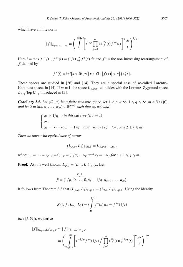
F. Cobos, T. Kühn / Journal of Functional Analysis 261 (2011) 3696–3722 3707
which have a finite norm
‖f ‖Lp,q;ν1,...,νm=
( μ(Ω)∫0
[t1/p
m∏j=1
LLνj
j (t)f ∗∗(t)]q
dt
t
)1/q
.
Here t = max{t,1/t}, f ∗∗(t) = (1/t)∫ t
0 f ∗(s) ds and f ∗ is the non-increasing rearrangement off defined by
f ∗(t) = inf{s > 0: μ
({x ∈ Ω:
∣∣f (x)∣∣ > s
})� t
}.
These spaces are studied in [26] and [14]. They are a special case of so-called Lorentz–Karamata spaces in [14]. If m = 1, the space Lp,q;ν1 coincides with the Lorentz–Zygmund spaceLp,q(logL)ν1 introduced in [3].
Corollary 3.5. Let (Ω,μ) be a finite measure space, let 1 < p < ∞,1 � q � ∞,m ∈ N ∪ {0}and let α = (α0, α1, . . . , αm) ∈ R
m+1 such that α0 = 0 and
⎧⎨⎩
α1 > 1/q (in this case we let r = 1),
or
α1 = · · · = αr−1 = 1/q and αr > 1/q for some 2 � r � m.
Then we have with equivalence of norms
(Lp,q,L1)α,q;K = Lp,q;ν1,...,νm,
where ν1 = · · · = νr−1 = 0, νr = (1/q) − αr and νj = −αj for r + 1 � j � m.
Proof. As it is well known, Lp,q = (L∞,L1)1/p,q . Let
ρ = (1/p,
r−1︷ ︸︸ ︷0, . . . ,0, αr − 1/q,αr+1, . . . , αm
).
It follows from Theorem 3.3 that (Lp,q,L1)α,q;K = (L∞,L1)ρ,q;K . Using the identity
K(t, f ;L∞,L1) = t
1/t∫0
f ∗(s) ds = f ∗∗(1/t)
(see [5,29]), we derive
‖f ‖(Lp,q ,L1)α,q;K ∼ ‖f ‖(L∞,L1)ρ,q;K
=( ∞∫ [
t−1/pf ∗∗(1/t)/ m∏
j=r
Lαj
j (t)L−1/qr (t)
]qdt
t
)1/q
Em(1)
3708 F. Cobos, T. Kühn / Journal of Functional Analysis 261 (2011) 3696–3722
∼( ∞∫Em(1)
[t−1/pf ∗∗(1/t)
/ m∏j=r
LLαj
j (t)LL−1/qr (t)
]qdt
t
)1/q
∼( E−1
m (1)∫0
[t1/pf ∗∗(t)
/ m∏j=r
LLαj
j (t)LL−1/qr (t)
]qdt
t
)1/q
∼( μ(Ω)∫
0
[t1/pLL(1/q)−αr
r (t)
m∏j=r+1
LL−αj
j (t)f ∗∗(t)]q
dt
t
)1/q
= ‖f ‖Lp,q;ν1,...,νm. �
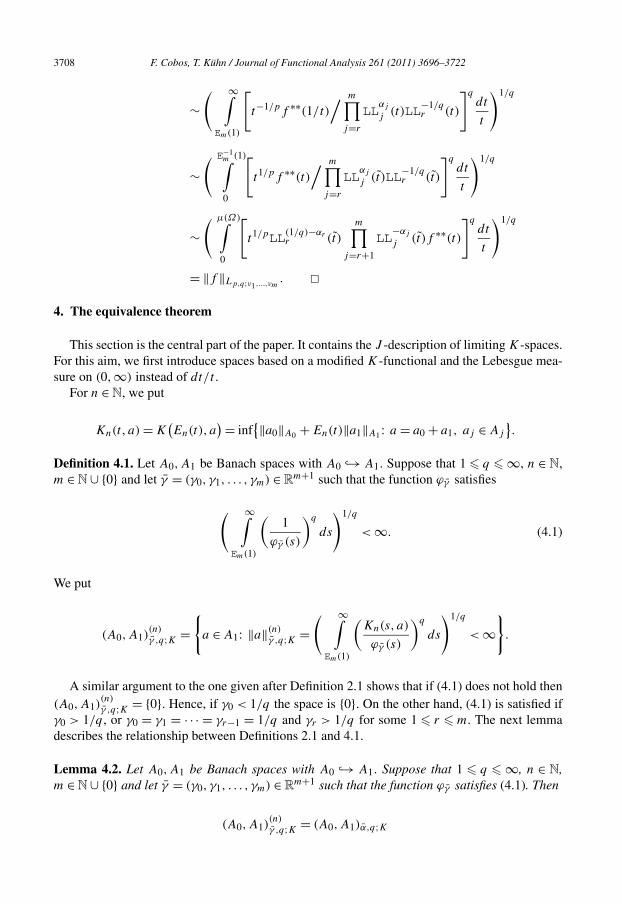
4. The equivalence theorem
This section is the central part of the paper. It contains the J -description of limiting K-spaces.For this aim, we first introduce spaces based on a modified K-functional and the Lebesgue mea-sure on (0,∞) instead of dt/t .
For n ∈ N, we put
Kn(t, a) = K(En(t), a
) = inf{‖a0‖A0 + En(t)‖a1‖A1 : a = a0 + a1, aj ∈ Aj
}.
Definition 4.1. Let A0,A1 be Banach spaces with A0 ↪→ A1. Suppose that 1 � q � ∞, n ∈ N,m ∈ N ∪ {0} and let γ = (γ0, γ1, . . . , γm) ∈ R
m+1 such that the function ϕγ satisfies
( ∞∫Em(1)
(1
ϕγ (s)
)q
ds
)1/q
< ∞. (4.1)
We put
(A0,A1)(n)γ ,q;K =
{a ∈ A1: ‖a‖(n)
γ ,q;K =( ∞∫Em(1)
(Kn(s, a)
ϕγ (s)
)q
ds
)1/q
< ∞}
.
A similar argument to the one given after Definition 2.1 shows that if (4.1) does not hold then(A0,A1)
(n)γ ,q;K = {0}. Hence, if γ0 < 1/q the space is {0}. On the other hand, (4.1) is satisfied if
γ0 > 1/q , or γ0 = γ1 = · · · = γr−1 = 1/q and γr > 1/q for some 1 � r � m. The next lemmadescribes the relationship between Definitions 2.1 and 4.1.
Lemma 4.2. Let A0,A1 be Banach spaces with A0 ↪→ A1. Suppose that 1 � q � ∞, n ∈ N,m ∈ N ∪ {0} and let γ = (γ0, γ1, . . . , γm) ∈ R
m+1 such that the function ϕγ satisfies (4.1). Then
(A0,A1)(n)γ ,q;K = (A0,A1)α,q;K
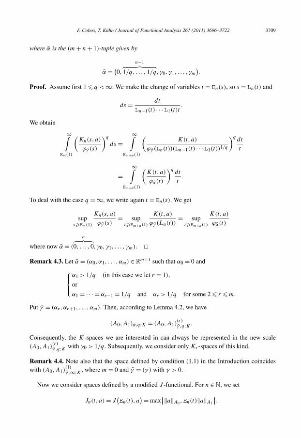
F. Cobos, T. Kühn / Journal of Functional Analysis 261 (2011) 3696–3722 3709
where α is the (m + n + 1)-tuple given by
α = (0,
n−1︷ ︸︸ ︷1/q, . . . ,1/q, γ0, γ1, . . . , γm
).
Proof. Assume first 1 � q < ∞. We make the change of variables t = En(s), so s = Ln(t) and
ds = dt
Ln−1(t) · · ·L1(t)t.
We obtain
∞∫Em(1)
(Kn(s, a)
ϕγ (s)
)q
ds =∞∫
Em+n(1)
(K(t, a)
ϕγ (Ln(t))(Ln−1(t) · · ·L1(t))1/q
)qdt
t
=∞∫
Em+n(1)
(K(t, a)
ϕα(t)
)qdt
t.
To deal with the case q = ∞, we write again t = En(s). We get
sups�Em(1)
Kn(s, a)
ϕγ (s)= sup
t�Em+n(1)
K(t, a)
ϕγ (Ln(t))= sup
t�Em+n(1)
K(t, a)
ϕα(t)
where now α = (
n︷ ︸︸ ︷0, . . . ,0, γ0, γ1, . . . , γm). �
Remark 4.3. Let α = (α0, α1, . . . , αm) ∈ Rm+1 such that α0 = 0 and⎧⎨
⎩α1 > 1/q (in this case we let r = 1),
or
α1 = · · · = αr−1 = 1/q and αr > 1/q for some 2 � r � m.
Put γ = (αr ,αr+1, . . . , αm). Then, according to Lemma 4.2, we have
(A0,A1)α,q;K = (A0,A1)(r)γ ,q;K.
Consequently, the K-spaces we are interested in can always be represented in the new scale(A0,A1)
(r)γ ,q;K with γ0 > 1/q. Subsequently, we consider only Kr -spaces of this kind.
Remark 4.4. Note also that the space defined by condition (1.1) in the Introduction coincideswith (A0,A1)
(1)γ ,∞;K , where m = 0 and γ = (γ ) with γ > 0.
Now we consider spaces defined by a modified J -functional. For n ∈ N, we set
Jn(t, a) = J(En(t), a
) = max{‖a‖A0,En(t)‖a‖A1
}.
3710 F. Cobos, T. Kühn / Journal of Functional Analysis 261 (2011) 3696–3722
Definition 4.5. Let A0,A1 be Banach spaces with A0 ↪→ A1, let 1 � q � ∞, n ∈ N, m ∈ N ∪ {0}and let δ = (δ0, δ1, . . . , δm) ∈ R
m+1. The space (A0,A1)(n)
δ,q;J is formed by all those a ∈ A1 which
can be represented by
a =∞∫
Em(1)
v(s) ds (convergence in A1) (4.2)
where v(s) is a strongly measurable function with values in A0 and
( ∞∫Em(1)
(Jn(s, v(s))
ϕδ(s)
)q
ds
)1/q
< ∞. (4.3)
We put
‖a‖(n)
δ,q;J = inf
{( ∞∫Em(1)
(Jn(s, v(s))
ϕδ(s)
)q
ds
)1/q}
where the infimum is taken over all v satisfying (4.2) and (4.3).
In order to compare the modified K- and J -spaces, we first prove a “limit version” of theso-called fundamental lemma of interpolation theory.
Lemma 4.6. Let A0,A1 be Banach spaces with A0 ↪→ A1, let n ∈ N and m ∈ N ∪ {0}. As-sume that a ∈ A1 with lims→∞ K(s, a)/s = 0. Then there is a strongly measurable functionv : [Em(1),∞) → A0 with
a =∞∫
Em(1)
v(s) ds (convergence in A1)
and
Jn
(s, v(s)
)� c
Kn(4s, a)
s, s � Em(1),
where c > 0 is a constant independent of a and v.
Proof. Choose r0 ∈ N such that 2r0−1 � Em(1) < 2r0 , set s0 = En(1) and for k ∈ N putsk = En(2k) and Ik = [sk−1, sk). Find vectors a0,k−1 ∈ A0 and a1,k−1 ∈ A1 with a = a0,k−1 +a1,k−1 and
‖a0,k−1‖A0 + sr0+k‖a1,k−1‖A1 � 2K(sr0+k, a).
F. Cobos, T. Kühn / Journal of Functional Analysis 261 (2011) 3696–3722 3711
Let
v0 = a0,0 and vk = a0,k − a0,k−1 for k ∈ N.
Then (vk−1) ⊆ A0 and
∥∥∥∥∥a −N∑
j=0
vj
∥∥∥∥∥A1
= ‖a − a0,N‖A1 = ‖a1,N‖A1 � 2K(sr0+N,a)
sr0+N
→ 0 as n → ∞.
Hence a = ∑∞k=1 vk−1, where the series converges in A1.
Next define
v(s) ={ v0
2r0 −Em(1)if s ∈ [Em(1),2r0),
vk
2r0+k−1 if s ∈ [2r0+k−1,2r0+k), k = 1,2, . . . .
It is clear that
∞∫Em(1)
v(s) ds =∞∑
k=1
vk−1 = a.
Moreover, for s ∈ [Em(1),2r0) we have
Jn
(s, v(s)
)� 1
2r0 − Em(1)Jn
(2r0, v0
)� 1
2r0 − Em(1)
[‖a0,0‖A0 + sr0‖a − a1,0‖A1
]� 1
2r0 − Em(1)
[2Kn
(2r0+1, a
)+ sr0‖a‖A1
]� c1
Kn(2r0+1, a)
2r0� c1
Kn(4s, a)
s.
For k ∈ N and s ∈ [2r0+k−1,2r0+k), we derive
Jn
(s, v(s)
)� 1
2r0+k−1Jn
(2r0+k, vk
)� 1
2r0+k−1
[‖a0,k‖A0 + ‖a0,k−1‖A0 + sr0+k
(‖a1,k‖A1 + ‖a1,k−1‖A1
)]� 4K(sr0+k+1, a)
2r0+k−1= 4Kn(2r0+k+1, a)
2r0+k−1
� 8Kn(4s, a)
s.
The proof is complete. �
3712 F. Cobos, T. Kühn / Journal of Functional Analysis 261 (2011) 3696–3722
Now we can establish the equivalence theorem between Kn- and Jn-spaces.
Theorem 4.7. Let A0,A1 be Banach spaces with A0 ↪→ A1. Suppose that 1 � q � ∞,n ∈ N, m ∈ N ∪ {0} and let γ = (γ0, γ1, . . . , γm) ∈ R
m+1 such that γ0 > 1/q . Let δ =(γ0 − 1, γ1, . . . , γm). Then we have with equivalent norms
(A0,A1)(n)γ ,q;K = (A0,A1)
(n)
δ,q;J .
Proof. For later use we note that the assumption on γ0 implies that ϕγ (s) = ∏∞j=0 Lj (s)
γj isequivalent to an increasing function and that there is a constant c1 > 0 with
ϕγ (2s) � c1ϕγ (s), s � Em(1). (4.4)
Take any a ∈ (A0,A1)(n)γ ,q;K. By Lemma 4.6, there is a strongly measurable function v(s) with
values in A0 such that
a =∞∫
Em(1)
v(s) ds with Jn
(s, v(s)
)� c
Kn(4s, a)
s, s � Em(1).
This inequality and (4.4) yield
( ∞∫Em(1)
(Jn(s, v(s))
ϕδ(s)
)q
ds
)1/q
� c
( ∞∫Em(1)
(Kn(4s, a)
sϕδ(s)
)q
ds
)1/q
= c
( ∞∫Em(1)
(Kn(4s, a)
ϕγ (s)
)q
ds
)1/q
� c2
( ∞∫Em(1)
(Kn(4s, a)
ϕγ (4s)
)q
ds
)1/q
� ‖a‖(n)γ ,q;K.
Therefore, a belongs to (A0,A1)(n)
δ,q;J with ‖a‖(n)
δ,q;J � ‖a‖(n)γ ,q;K.
Take now a ∈ (A0,A1)(n)
δ,q;J and let a = ∫ ∞Em(1)
v(s) ds be a Jn-representation of a with
( ∞∫Em(1)
(Jn(s, v(s))
ϕδ(s)
)q
ds
)1/q
� 2‖a‖(n)
δ,q;J .
We have
F. Cobos, T. Kühn / Journal of Functional Analysis 261 (2011) 3696–3722 3713
Kn(t, a) �∞∫
Em(1)
Kn
(t, v(s)
)ds
�∞∫
Em(1)
min{1,En(t)/En(s)
}Jn
(s, v(s)
)ds
=t∫
Em(1)
Jn
(s, v(s)
)ds + En(t)
∞∫t
Jn(s, v(s))
En(s)ds.
Thus
‖a‖(n)γ ,q;K =
( ∞∫Em(1)
(Kn(t, a)
ϕγ (t)
)q
dt
)1/q
�( ∞∫Em(1)
(1
ϕγ (t)
t∫Em(1)
Jn
(s, v(s)
)ds
)q
dt
)1/q
+( ∞∫Em(1)
(En(t)
ϕγ (t)
∞∫t
Jn(s, v(s))
En(s)ds
)q
dt
)1/q
= I1 + I2.
We first estimate I1. Choose ε > 0 such that ρ = γ0 − ε > 1/q . Using Hölder’s inequality, weget
t∫Em(1)
Jn
(s, v(s)
)ds �
( t∫Em(1)
(Jn(s, v(s))
ϕδ(s)sε
)q
ds
)1/q( t∫Em(1)
(ϕδ(s)
sε
)q ′
ds
)1/q ′
=( t∫Em(1)
(Jn(s, v(s))
ϕδ(s)sε
)q
ds
)1/q( t∫Em(1)
(ϕγ (s)
s1+ε
)q ′
ds
)1/q ′
.
Since ρ < γ0, the function ϕγ (s)/sρ is equivalent to an increasing function. It follows that
( t∫Em(1)
(ϕγ (s)
sρ· 1
s1+ε−ρ
)q ′
ds
)1/q ′
� ϕγ (t)
tρt
1q′ −1−ε+ρ = ϕγ (t)t
−ε− 1q .
Consequently,
3714 F. Cobos, T. Kühn / Journal of Functional Analysis 261 (2011) 3696–3722
I1 �( ∞∫Em(1)
t−εq−1
[ t∫Em(1)
(Jn(s, v(s))
ϕδ(s)sε
)q
ds
]dt
)1/q
=( ∞∫Em(1)
(Jn(s, v(s))
ϕδ(s)sε
)q( ∞∫
s
t−εq−1 dt
)ds
)1/q
∼( ∞∫Em(1)
(Jn(s, v(s))
ϕδ(s)
)q
ds
)1/q
� 2‖a‖(n)
δ,q;J .
Next we proceed with I2. First we consider the case q = 1. We have
I2 =∞∫
Em(1)
Jn(s, v(s))
En(s)
( s∫Em(1)
En(t)
ϕγ (t)dt
)ds.
The second integral behaves like En(s)/ϕγ (s) because En(t)/et/2ϕγ (t) is equivalent to an increas-
ing function and so
s∫Em(1)
En(t)
et/2ϕγ (t)et/2 dt � En(s)
es/2ϕγ (s)
s∫Em(1)
et/2 dt � En(s)
ϕγ (s).
It follows that
I2 �∞∫
Em(1)
Jn(s, v(s))
ϕγ (s)ds �
∞∫Em(1)
sJn(s, v(s))
ϕγ (s)ds
=∞∫
Em(1)
Jn(s, v(s))
ϕδ(s)ds � 2‖a‖(n)
δ,1;J .
Suppose now that 1 < q � ∞. By Hölder’s inequality we derive
I2 �( ∞∫Em(1)
[En(t)
ϕγ (t)
( ∞∫t
(Jn(s, v(s))
ϕδ(s)
)q
ds
)1/q( ∞∫t
(ϕδ(s)
En(s)
)q ′
ds
)1/q ′]q
dt
)1/q
� 2
( ∞∫Em(1)
[En(t)
ϕγ (t)
( ∞∫t
(ϕδ(s)
En(s)
)q ′
ds
)1/q ′]q
dt
)1/q
‖a‖(n)
δ,q;J .
Since es/2ϕ ¯(s)/En(s) is equivalent to a decreasing function, the inner integral behaves like
δ
F. Cobos, T. Kühn / Journal of Functional Analysis 261 (2011) 3696–3722 3715
ϕδ(t)/En(t) and so
I2 � 2
( ∞∫Em(1)
t−q dt
)1/q
‖a‖(n)
δ,q;J .
The last integral is finite because 1 < q � ∞. Consequently,
‖a‖(n)γ ,q;K � I1 + I2 � ‖a‖(n)
δ,q;J .
This completes the proof. �Next we show the relation of Jn-spaces to the usual J -spaces.
Lemma 4.8. Let A0,A1 be Banach spaces with A0 ↪→ A1. Suppose that 1 � q � ∞, n ∈ N,m ∈ N ∪ {0} and let β = (β0, β1, . . . , βm) ∈ R
m+1. Then
(A0,A1)(n)
β,q;J = (A0,A1)ρ,q;J
where ρ is the (m + n + 1)-tuple given by ρ = (0,
n−1︷ ︸︸ ︷−1/q ′, . . . ,−1/q ′, β0, β1, . . . , βm).
Proof. Let a = ∫ ∞Em(1)
v(s) ds. Making the change of variable s = Ln(t) with
ds = dt/Ln−1(t) · · ·L1(t)t
we obtain
a =∞∫
Em+n(1)
v(Ln(t))
Ln−1(t) · · ·L1(t)
dt
t=
∞∫Em+n(1)
u(t)dt
t
where
u(t) = v(Ln(t)
)/Ln−1(t) · · ·L1(t).
Moreover, if q = ∞, we have
sups�Em(1)
Jm(s, v(s))
ϕβ(s)= sup
t�Em+n(1)
J (t, v(Ln(t)))
ϕβ(Ln(t))
= supt�Em+n(1)
J (t, u(t))
ϕβ(Ln(t))(Ln−1(t) · · ·L1(t))−1
= supJ (t, u(t))
ϕρ(t).
t�Em+n(1)
3716 F. Cobos, T. Kühn / Journal of Functional Analysis 261 (2011) 3696–3722
Similarly, for 1 � q < ∞, we derive
∞∫Em(1)
(Jn(s, v(s))
ϕβ(s)
)q
ds =∞∫
Em+n(1)
(J (t, u(t))
ϕβ(Ln(t))[Ln−1(t) · · ·L1(t)]−1
)qdt
Ln−1(t) · · ·L1(t)t
=∞∫
Em+n(1)
(J (t, u(t))
ϕρ(t)
)qdt
t.
This yields that (A0,A1)(n)
β,q;J ↪→ (A0,A1)ρ,q;J .
To check the converse inclusion, take any a ∈ (A0,A1)ρ,q;J with J -representation a =∫ ∞Em+n(1)
u(t) dtt. We make the change of variable t = En(s) with ds = dt/Ln−1(t) · · ·L1(t)t. Put
v(s) = u(En(s))En−1(s) · · ·E1(s). Then
a =∞∫
Em(1)
u(En(s)
)En−1(s) · · ·E1(s) ds =
∞∫Em(1)
v(s) ds.
Moreover,
∞∫Em+n(1)
(J (t, u(t))
ϕρ(t)
)qdt
t=
∞∫Em(1)
(Jn(s, v(s))
ϕρ(En(s))∏n−1
k=1 Ek(s)
)q n−1∏k=1
Ek(s) ds
=∞∫
Em(1)
(Jn(s, v(s))
ϕβ(s)
)q
ds.
This completes the proof. �Now we establish the equivalence theorem for limiting K-spaces.
Corollary 4.9. Let A0,A1 be Banach spaces with A0 ↪→ A1, let 1 � q � ∞, m ∈ N ∪ {0} andsuppose that α = (α0, α1, . . . , αm) ∈ R
m+1 with α0 = 0 and
⎧⎨⎩
α1 > 1/q (in this case we let r = 1),
or
α1 = · · · = αr−1 = 1/q and αr > 1/q for some 2 � r � m.
Then we have with equivalent norms
(A0,A1)α,q;K = (A0,A1)β,q;J
where β = (0,
r−1︷ ︸︸ ︷−1/q ′, . . . ,−1/q ′, αr − 1, αr+1, . . . , αm).
F. Cobos, T. Kühn / Journal of Functional Analysis 261 (2011) 3696–3722 3717
Proof. Let γ = (αr ,αr+1, . . . , αm) ∈ Rm−r+1 and ω = (αr −1, αr+1, . . . , αm) ∈ R
m−r+1. UsingLemma 4.2, Theorem 4.7 and Lemma 4.8, we derive
(A0,A1)α,q;K = (A0,A1)(r)γ ,q;K = (A0,A1)
(r)ω,q;J = (A0,A1)β,q;J . �
Corollary 4.9 shows that in the equivalence theorem for the limiting case, it is needed thecorrection factor
Ψ (t) =r∏
j=1
Lj (t)
which depends on the logarithms that define the K-space but it does not depend on the Lq -norm:Condition
K(t, a)∏mj=1 Lj (t)
αj∈ Lq
(dt
t
)
is equivalent to the fact that a can be J -represented by some u(t) such that
Ψ (t)J (t, u(t))∏mj=1 Lj (t)
αj∈ Lq
(dt
t
).
As a direct consequence we get the following J -description for the K-spaces mentioned inthe Introduction.
Corollary 4.10. Let A0,A1 be Banach spaces with A0 ↪→ A1, let 1 � q � ∞, α > 0 and ρ >
1/q. Then we have with equivalent norms
(A0,A1)(0,α),∞;K = (A0,A1)(0,α−1),∞;J ,
and
(A0,A1)(0,1/q,ρ),q;K = (A0,A1)(0,−1/q ′,ρ−1),q;J .
For q < ∞ we have also the following density result.
Corollary 4.11. Let A0,A1 be Banach spaces with A0 ↪→ A1, let 1 � q < ∞, m ∈ N ∪ {0} andsuppose that α = (α0, α1, . . . , αm) ∈ R
m+1 with α0 = 0 and α1 > 1/q , or α0 = 0, α1 = · · · =αr−1 = 1/q and αr > 1/q for some 2 � r � m. Then A0 is dense in (A0,A1)α,q;K .
Proof. By Corollary 4.9, we have with equivalence of norms (A0,A1)α,q;K = (A0,A1)β,q;J
where β = (0,
r−1︷ ︸︸ ︷−1/q ′, . . . ,−1/q ′, αr −1, αr+1, . . . , αm). Take any a ∈ (A0,A1)β,q;J and let a =∫ ∞
u(t) dt/t be a J -representation of a. Given any ε > 0, since q < ∞, it follows from (2.5)
Em(1)
3718 F. Cobos, T. Kühn / Journal of Functional Analysis 261 (2011) 3696–3722
that there is s > Em(1) such that
( ∞∫s
(J (t, u(t))
ϕβ(t)
)qdt
t
)1/q
< ε.
Moreover
s∫Em(1)
∥∥u(t)∥∥
A0
dt
t�
s∫Em(1)
J (t, u(t))
ϕβ(t)ϕβ(t)
dt
t
�( s∫Em(1)
(J (t, u(t))
ϕβ(t)
)qdt
t
)1/q( s∫Em(1)
ϕβ(t)q′ dt
t
)1/q ′
< ∞
because ϕβ(t)q′/t is a continuous function. Let w = ∫ s
Em(1)u(t) dt/t. Then we have that w ∈ A0
with a − w = ∫ ∞s
u(t) dt/t and
‖a − w‖β,q;J �( ∞∫
s
(J (t, u(t))
ϕβ(t)
)qdt
t
)1/q
< ε. �
5. Remarks on approximation of stochastic integrals
In this last section we will show some complements to the results of C. Geiss, S. Geiss andM. Hujo [19,20]. Let F be a Banach space, let (λn) be a sequence of positive numbers and1 � q � ∞. We define �q(λnF ) as the collection of all sequences x = (xn) ⊆ F having a finitenorm
‖x‖�q(λnF ) =( ∞∑
n=1
(λn‖xn‖F
)q)1/q
.
We are interested in interpolation properties of the couple (�q(n1/2F), �q(F )).Since for any x = (xn) ∈ �∞(F ) we have
K(t, x;�q
(n1/2F
), �q(F )
) =( ∞∑
n=1
(min
{n1/2, t
}‖xn‖F
)q)1/q
, (5.1)
we can proceed as in the scalar case (see Theorem 3.2 and Corollary 3.3) and obtain, for1 � q � ∞ and α > 1/q , the formula
(�q
(n1/2F
), �q(F )
)(0,α),q;K = �q
(n1/2(1 + logn)(1/q)−αF
). (5.2)
The following result refers to the non-diagonal case.
F. Cobos, T. Kühn / Journal of Functional Analysis 261 (2011) 3696–3722 3719
Theorem 5.1. Let F be a Banach space, let 1 � q < ∞ and α > 1/q . Then
(�∞
(n1/2F
), �∞(F )
)(0,α),q;K ↪→ �q
(n1/2−1/q(1 + logn)−αF
)∩ �∞(n1/2(1 + logn)1/q−αF
).
Proof. Let x = (xn) ∈ �∞(F ). Fix n ∈ N and let t � n1/2. By (5.1), we have
K(t, x) � n1/2‖xn‖F .
Whence
‖x‖(0,α),q;K ∼( ∞∫
1
(K(t, x)
LLα1 (t)
)qdt
t
)1/q
� n1/2‖xn‖F
( ∞∫n
dt
LLαq
1 (t)t
)1/q
� n1/2(1 + logn)(1/q)−α‖xn‖F .
Taking the supremum over n ∈ N we obtain
(�∞
(n1/2F
), �∞(F )
)(0,α),q;K ↪→ �∞
(n1/2(1 + logn)1/q−αF
).
On the other hand, since K(t, x) � n1/2‖xn‖F for n1/2 � t < (n + 1)1/2, we derive
‖x‖q
(0,α),q;K ∼∞∫
1
(K(t, x)
LLα1 (t)
)qdt
t
�∞∑
n=1
(n1/2‖xn‖F
)q (n+1)1/2∫n1/2
dt
LLαq
1 (t)t
�∞∑
n=1
(n1/2‖xn‖F
)q 1
n1/2
1
n1/2LLαq
1 (n)
=∞∑
n=1
(n1/2−1/q(1 + logn)−α‖xn‖F
)q.
This shows that
(�∞
(n1/2F
), �∞(F )
)(0,α),q;K ↪→ �q
(n1/2−1/q(1 + logn)−αF
)and completes the proof. �
3720 F. Cobos, T. Kühn / Journal of Functional Analysis 261 (2011) 3696–3722
Remark 5.2. Note that the spaces
A = �q
(n1/2−1/q(1 + logn)−α
), B = �∞
(n1/2(1 + logn)1/q−α
)are not comparable. Indeed, take any N ∈ N and consider the sequence x = (xn) defined by
xn ={
n1/q−1/2(1 + logn)α for n � N,
0 else.
Then ‖x‖A = (∑N
n=1 1)1/q = N1/q but
‖x‖B = max1�n�N
(n(1 + logn)
)1/q = N1/q(1 + logN)1/q .
So A is not continuously embedded in B . On the other hand, take the sequence y = (yn) definedby yn = n−1/2(1 + logn)α−1/q . Clearly y belongs to B with ‖y‖B = 1, but it does not belong toA because
∞∑n=1
(n1/2−1/q(1 + logn)−αyn
)q =∞∑
n=1
1
n(1 + logn)= ∞.
In order to relate the previous results on limiting interpolation spaces to approximation ofstochastic integrals, let γ be the standard Gaussian measure on the real line, let (hn)
∞n=1 be the
orthonormal basis of L2(γ ) given by Hermite polynomials and consider the Sobolev space
D1,2(γ ) ={
f =∞∑
n=1
λnhn ∈ L2(γ ): ‖f ‖D1,2(γ ) =( ∞∑
n=1
(n + 1)λ2n
)1/2
< ∞}
.
By real interpolation in the ordered couple (D1,2(γ ),L2(γ )) we obtain the Besov spacesB1−θ
2,q (γ ) = (D1,2(γ ),L2(γ ))θ,q (see [29,5,30]). Besov spaces with a more general smoothnesshave been also considered in the literature to deal with a number of problems in function spaces(see, for example, [8,31,32,11]). We are interested here in limiting Besov spaces generated bythe ((0, α), q;K)-method with α > 1/q
B1,α2,q (γ ) = (
D1,2(γ ),L2(γ ))(0,α),q;K. (5.3)
The following result is a consequence of (5.3), Theorem 5.1 and the interpolation property (The-orem 3.1).
Corollary 5.3. Let T : L2(γ ) → �∞(L2(γ )) be a bounded linear operator such that the restric-tion to D1,2(γ ) defines a bounded operator T : D1,2(γ ) → �∞(
√nL2(γ )). If 1 � q � ∞ and
α > 1/q , then the restrictions
T : B1,α2,q (γ ) → �q
(n1/2−1/q(1 + logn)−αL2(γ )
),
T : B1,α2,q (γ ) → �∞
(n1/2(1 + logn)1/q−αL2(γ )
)are bounded.
F. Cobos, T. Kühn / Journal of Functional Analysis 261 (2011) 3696–3722 3721
Corollary 5.3 allows us to complement the results by C. Geiss, S. Geiss and M. Hujo [19,20]on approximation of stochastic integrals using deterministic equidistant nets of cardinality n+ 1.They showed, in particular, that for f ∈ D1,2(γ ) the optimal approximation rate n−1/2 is attained,while for f ∈ B1−θ
2,∞(γ ) with 0 < θ < 1 the rate is only n−1/2+θ/2.In the limiting case θ = 0, Corollary 5.3 provides additional information. Indeed, by our result
and the arguments given in [20, pp. 226–227], it follows that for f ∈ B1,α2,∞(γ ) with α > 0 the
approximation rate is n−1/2(1+ logn)α , so the optimal rate n−1/2 is achieved up to a logarithmicfactor.
References
[1] I. Ahmed, D.E. Edmunds, W.D. Evans, G.E. Karadzhov, Reiteration theorems for the K-interpolation method inlimiting cases, Math. Nachr. 284 (2011) 421–442.
[2] W.O. Amrein, A. Boutet de Monvel, V. Georgescu, C0-Groups, Commutator Methods and Spectral Theory of N -Body Hamiltonians, Progr. Math., vol. 135, Birkhäuser, Basel, 1996.
[3] C. Bennett, K. Rudnick, On Lorentz–Zygmund spaces, Dissertationes Math. 175 (1980) 1–67.[4] C. Bennett, R. Sharpley, Interpolation of Operators, Academic Press, Boston, 1988.[5] J. Bergh, J. Löfström, Interpolation Spaces. An Introduction, Springer, Berlin, 1976.[6] Yu.A. Brudnyı, N.Ya. Krugljak, Interpolation Functors and Interpolation Spaces, vol. 1, North-Holland, Amsterdam,
1991.[7] P.L. Butzer, H. Berens, Semi-Groups of Operators and Approximation, Springer, New York, 1967.[8] F. Cobos, D.L. Fernandez, Hardy–Sobolev spaces and Besov spaces with a function parameter, in: Function Spaces
and Applications, in: Lecture Notes in Math., vol. 1302, Springer, Berlin, 1988, pp. 158–170.[9] F. Cobos, L.M. Fernández-Cabrera, T. Kühn, T. Ullrich, On an extreme class of real interpolation spaces, J. Funct.
Anal. 256 (2009) 2321–2366.[10] F. Cobos, L.M. Fernández-Cabrera, M. Mastyło, Abstract limit J -spaces, J. London Math. Soc. (2) 82 (2010) 501–
525.[11] F. Cobos, T. Kühn, Approximation and entropy numbers in Besov spaces of generalized smoothness, J. Approx.
Theory 160 (2009) 56–70.[12] A. Connes, Noncommutative Geometry, Academic Press, San Diego, 1994.[13] R.Ya. Doktorskii, Reiteration relations of the real interpolation method, Soviet Math. Dokl. 44 (1992) 665–669.[14] D.E. Edmunds, W.D. Evans, Hardy Operators, Function Spaces and Embeddings, Springer, Berlin, 2004.[15] W.D. Evans, B. Opic, Real interpolation with logarithmic functors and reiteration, Canad. J. Math. 52 (2000) 920–
960.[16] W.D. Evans, B. Opic, L. Pick, Real interpolation with logarithmic functors, J. Inequal. Appl. 7 (2002) 187–
269.[17] P. Fernández-Martínez, T. Signes, Real interpolation with symmetric spaces and slowly varying functions, Q. J.
Math. (2010), doi:10.1093/qmath/haq009, in press.[18] S. Geiss, Private communication, September 2009.[19] C. Geiss, S. Geiss, On approximation of a class of stochastic integrals and interpolation, Stoch. Stoch. Rep. 76
(2004) 339–362.[20] S. Geiss, M. Hujo, Interpolation and approximation in L2(γ ), J. Approx. Theory 144 (2007) 213–232.[21] A. Gogatishvili, B. Opic, W. Trebels, Limiting reiteration for real interpolation with slowly varying functions, Math.
Nachr. 278 (2005) 86–107.[22] M.E. Gomez, M. Milman, Extrapolation spaces and almost-everywhere convergence of singular integrals, J. London
Math. Soc. 34 (1986) 305–316.[23] J. Gustavsson, A function parameter in connection with interpolation of Banach spaces, Math. Scand. 42 (1978)
289–305.[24] S. Janson, Minimal and maximal methods of interpolation, J. Funct. Anal. 44 (1981) 50–73.[25] M. Milman, Extrapolation and Optimal Decompositions, Lecture Notes in Math., vol. 1580, Springer, Berlin,
1994.[26] B. Opic, L. Pick, On generalized Lorentz–Zygmund spaces, Math. Inequal. Appl. 2 (1999) 391–467.[27] J. Peetre, A Theory of Interpolation of Normed Spaces, Notas Mat., vol. 39, Inst. Mat. Pura Apl., Rio de Janeiro,
1968.
3722 F. Cobos, T. Kühn / Journal of Functional Analysis 261 (2011) 3696–3722
[28] L.-E. Persson, Interpolation with a parameter function, Math. Scand. 59 (1986) 199–222.[29] H. Triebel, Interpolation Theory, Function Spaces, Differential Operators, North-Holland, Amsterdam, 1978.[30] H. Triebel, Theory of Function Spaces, Birkhäuser, Basel, 1983.[31] H. Triebel, The Structure of Functions, Birkhäuser, Basel, 2001.[32] H. Triebel, Theory of Function Spaces III, Birkhäuser, Basel, 2006.


![Tameness on the boundary and Ahlfors’ measure conjecture · 1(N) [Bon2], obviating any need for limiting arguments. Using Bonahon’s work, Canary established the equivalence of](https://img.pdfslide.us/doc/110x75/600b086b67a29a4eb23b4795/tameness-on-the-boundary-and-ahlforsa-measure-conjecture-1n-bon2-obviating.jpg)