Embed Size (px)
Citation preview
Artificial Intelligence 147 (2003) 163–223
www.elsevier.com/locate/artint
Equivalence notions and model minimization inMarkov decision processes
Robert Givan a,∗, Thomas Dean b, Matthew Greig a
a School of Electrical and Computer Engineering, Purdue University, West Lafayette, IN 47907, USAb Department of Computer Science, Brown University, Providence, RI 02912, USA
Received 22 June 2001; received in revised form 17 April 2002
Abstract
Many stochastic planning problems can be represented using Markov Decision Processes (MDPs).A difficulty with using these MDP representations is that the common algorithms for solvingthem run in time polynomial in the size of the state space, where this size is extremely large formost real-world planning problems of interest. Recent AI research has addressed this problem byrepresenting the MDP in a factored form. Factored MDPs, however, are not amenable to traditionalsolution methods that call for an explicit enumeration of the state space. One familiar way to solveMDP problems with very large state spaces is to form a reduced (or aggregated) MDP with thesame properties as the original MDP by combining “equivalent” states. In this paper, we discussapplying this approach to solving factored MDP problems—we avoid enumerating the state spaceby describing large blocks of “equivalent” states in factored form, with the block descriptions beinginferred directly from the original factored representation. The resulting reduced MDP may haveexponentially fewer states than the original factored MDP, and can then be solved using traditionalmethods. The reduced MDP found depends on the notion of equivalence between states used inthe aggregation. The notion of equivalence chosen will be fundamental in designing and analyzingalgorithms for reducing MDPs. Optimally, these algorithms will be able to find the smallest possiblereduced MDP for any given input MDP and notion of equivalence (i.e., find the “minimal model” forthe input MDP). Unfortunately, the classic notion of state equivalence from non-deterministic finitestate machines generalized to MDPs does not prove useful. We present here a notion of equivalencethat is based upon the notion of bisimulation from the literature on concurrent processes. Ourgeneralization of bisimulation to stochastic processes yields a non-trivial notion of state equivalencethat guarantees the optimal policy for the reduced model immediately induces a correspondingoptimal policy for the original model. With this notion of state equivalence, we design and analyze
* Corresponding author.E-mail addresses: [email protected] (R. Givan), [email protected] (T. Dean), [email protected]
(M. Greig).
0004-3702/03/$ – see front matter 2003 Elsevier Science B.V. All rights reserved.
doi:10.1016/S0004-3702(02)00376-4
164 R. Givan et al. / Artificial Intelligence 147 (2003) 163–223
an algorithm that minimizes arbitrary factored MDPs and compare this method analytically to
previous algorithms for solving factored MDPs. We show that previous approaches implicitly deriveequivalence relations that we define here. 2003 Elsevier Science B.V. All rights reserved.Keywords: Markov decision processes; State abstraction; Stochastic planning; Bisimulation; Knowledgerepresentation; Factored state spaces
1. Introduction
Discrete state planning problems can be described semantically by a state-transitiongraph (or model), where the vertices correspond to the states of the system, and the edgesare possible state transitions resulting from actions. These models, while often large, canbe efficiently represented, e.g., with factoring, without enumerating the states.
Well-known algorithms have been developed to operate directly on these models,including methods for determining reachability, finding connecting paths, and computingoptimal policies. Some examples are the algorithms for solving Markov decision processes(MDPs) that are polynomial in the size of the state space [42]. MDPs provide a formalbasis for representing planning problems that involve actions with stochastic results [8].A planning problem represented as an MDP is given by four objects: (1) a space of possibleworld states, (2) a space of possible actions that can be performed, (3) a real-valued rewardfor each action taken in each state, and (4) a transition probability model specifying foreach action α and each state p the distribution over resulting states for performing actionα in state p.
Typical planning MDPs have state spaces that are astronomically large, exponential inthe number of state variables. In planning the assembly of a 1000-part device, potentialstates could allow any subset of the parts to be “in the closet”, giving at least 21000 states.In reaction, AI researchers have for decades resorted to factored state representations—rather than enumerate the states, the state space is specified with a set of finite-domainstate variables. The state space is the set of possible assignments to these variables, and,though never enumerated, is well defined. Representing action-transition distributionswithout enumerating states, using dynamic Bayesian networks [13], further increasesrepresentational efficiency. These networks exploit independence properties to compactlyrepresent probability distributions.
Planning systems using these compact representations must adopt algorithms thatreason about the model at the symbolic level, and thus reason about large groups of statesthat behave identically with respect to the action or properties under consideration, e.g.,[18,36]. These systems incur a significant computational cost by deriving and re-derivingthese groupings repeatedly over the course of planning. Factored MDP representationsexploit similarities in state behaviors to achieve a compact representation. Unfortunately,this increase in compactness representing the MDP provably does not always translate intoa similar increase in efficiency when computing the solution to that MDP [35]. In particular,states grouped together by the problem representation may behave differently when actionsequences are applied, and thus may need to be separated during solution—leading to a
R. Givan et al. / Artificial Intelligence 147 (2003) 163–223 165
need to derive further groupings of states during solution. Traditional operations-research
solution methods do not address these issues, applying only to the explicit original MDPmodel.Recent AI research has addressed this problem by giving algorithms that in each caseamount to state space aggregation algorithms [1,4,5,7,12,15,16,32]—reasoning directlyabout the factored representation to find blocks of states that are equivalent to each other.In this work, we reinterpret these approaches in terms of partitioning the state space intoblocks of equivalent states, and then building a smaller explicit MDP, where the statesin the smaller MDP are the blocks of equivalent states from the partition of the originalMDP state space. The smaller MDP can be shown to be equivalent to the original ina well-defined sense, and is amenable to traditional solution techniques. Typically, analgorithm for solving an MDP that takes advantage of an implicit (i.e., factored) state-space representation, such as [9], can be alternatively viewed as transforming the problemto a reduced MDP, and then applying a standard MDP-solving algorithm to the explicitstate space of the reduced MDP.
One of our contributions is to describe a useful notion of state equivalence. This notionis a generalization of the notion of bisimulation from the literature on the semanticsof concurrent processes [23,37]. Generalized to the stochastic case for MDP states, wecall this equivalence relation stochastic bisimilarity. Stochastic bisimilarity is similar to aprevious notion from the probabilistic transition systems literature [30], with the differencebeing the incorporation of reward.
We develop an algorithm that performs the symbolic manipulations necessary to groupequivalent states under stochastic bisimilarity. Our algorithm is based on the iterativemethods for finding a bisimulation in the semantics of concurrent processes literature [23,37]. The result of our algorithm is a model of (possibly) reduced size whose states (calledblocks or aggregates) correspond to groups of states in the original model. The aggregatesare described symbolically. We prove that the reduced model constitutes a reformulationof the original model: any optimal policy in the reduced MDP generalizes to an optimalpolicy in the original MDP.
If the operations required for manipulating the aggregates can each be done in constanttime then our algorithm runs in time polynomial in the number of states in the reducedmodel. However, the aggregate manipulation problems, with general propositional logicas the representation are NP-hard, and so, generally speaking, aggregate manipulationoperations do not run in constant time. One way to attempt to make the manipulationoperations fast is to limit the expressiveness of the representation for the aggregates—when a partition is called for that cannot be represented, we use some refinement of thatpartition by splitting aggregates as needed to stay within the representation. Using suchrepresentations, the manipulation operations are generally more tractable, however thereduced MDP state space may grow in size due to the extra aggregate splitting required.Previous algorithms for manipulating factored models implicitly compute reduced modelsunder restricted representations. This issue leads to an interesting trade-off between thestrength of the representation used to define the aggregates (affecting the size of the reducedMDP), and the cost of manipulation operations. Weak representations lead to poor modelreduction, but expressive representations lead to expensive operations (as shown, e.g., in[14,19]).
166 R. Givan et al. / Artificial Intelligence 147 (2003) 163–223
The basic idea of computing equivalent reduced processes has its origins in automata
theory [22] and stochastic processes [27], and has been applied more recently in modelchecking in computer-aided verification [10,31]. Our model minimization algorithm canbe viewed as building on the work of [31] by generalizing non-deterministic transitions tostochastic transitions and introducing a notion of utility.We claim a number of contributions for this paper. First, we develop a notion ofequivalence between MDP states that relates the literatures on automata theory, concurrentprocess semantics, and decision theory. Specifically, we develop a useful variant of thenotion of bisimulation, from concurrent processes, for MDPs. Second, we show thatthe mechanisms for computing bisimulations from the concurrent processes literaturegeneralize naturally to MDPs and can be carried out on factored representations, withoutenumerating the state space. Third, we show that state aggregation (in factored form),using automatically detected stochastic bisimilarity, results in a (possibly) reduced model,and we prove that solutions to this reduced model (which can be found with traditionalmethods) apply when lifted to the original model. Finally, we carefully compare previousalgorithms for solving factored MDPs to the approach of computing a minimal modelunder some notion of state equivalence (stochastic bisimilarity or a refinement thereof)and then applying a traditional MDP-solving technique to the minimal model.
Section 2 discusses the relevant background material. Section 3 presents some candidatenotions of equivalence between states in an MDP, including stochastic bisimulation, andSection 4 builds an algorithm for computing the minimal model for an MDP understochastic bisimulation. Section 5 compares existing algorithms for working with afactored MDP to our approach. Section 6 covers extensions to this work to handle largeaction spaces and to select reduced models approximately. Section 7 shows brief empiricalresults, and the remaining section draws some conclusions. The proofs of our results appearin the appendix, except where noted in the main text.
2. Background material
2.1. Sequential decision problems
2.1.1. Finite sequential machinesA non-deterministic finite sequential machine (FSM) F (adapted from [22]) is a tuple
〈Q,A,O,T ,R〉 where Q is a finite set of states, A is a finite set of inputs (actions), andO is a set of possible outputs. The transition function, T , is a subset of Q× A×Q thatidentifies the allowable transitions for each input in each state. The output function, R,is a mapping from Q to O giving for each state the output generated when transitioninginto that state. We say that a state sequence q0, . . . , qk is possible under inputs α1, . . . , αkfrom A when T contains all tuples of the form 〈qx−1, αx, qx〉. We say that q0, . . . , qk cangenerate output sequence o1, . . . , ok when R maps each qx for x > 0 to ox . We can thensay that o1, . . . , ok is a possible output sequence when following input sequence α1, . . . , αkfrom start state q0 if o1, . . . , ok can be generated from some state sequence q0, . . . , qkpossible under α1, . . . , αk . Finally, we denote an input sequence as ξ , an output sequence
R. Givan et al. / Artificial Intelligence 147 (2003) 163–223 167
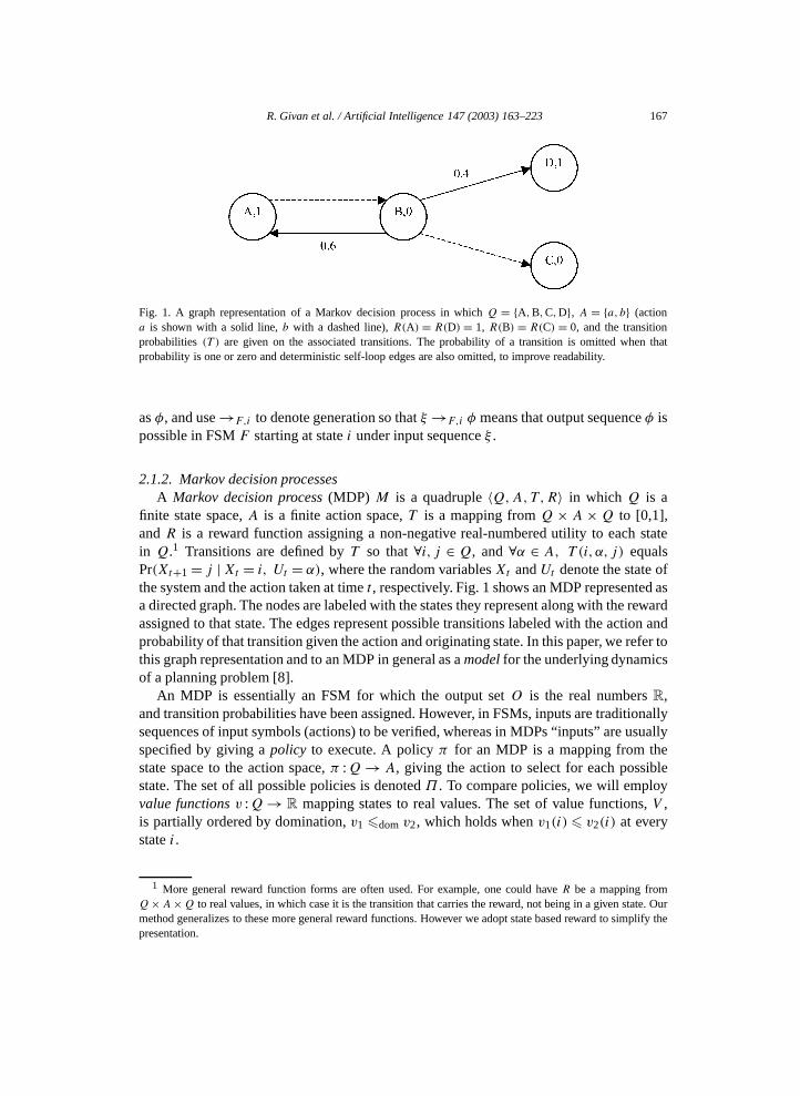
Fig. 1. A graph representation of a Markov decision process in which Q = {A,B,C,D}, A = {a,b} (actiona is shown with a solid line, b with a dashed line), R(A) = R(D) = 1, R(B) = R(C) = 0, and the transitionprobabilities (T ) are given on the associated transitions. The probability of a transition is omitted when thatprobability is one or zero and deterministic self-loop edges are also omitted, to improve readability.
as φ, and use →F,i to denote generation so that ξ →F,i φ means that output sequence φ ispossible in FSM F starting at state i under input sequence ξ .
2.1.2. Markov decision processesA Markov decision process (MDP) M is a quadruple 〈Q,A,T ,R〉 in which Q is a
finite state space, A is a finite action space, T is a mapping from Q × A ×Q to [0,1],and R is a reward function assigning a non-negative real-numbered utility to each statein Q.1 Transitions are defined by T so that ∀i, j ∈ Q, and ∀α ∈ A, T (i,α, j) equalsPr(Xt+1 = j |Xt = i, Ut = α), where the random variables Xt and Ut denote the state ofthe system and the action taken at time t , respectively. Fig. 1 shows an MDP represented asa directed graph. The nodes are labeled with the states they represent along with the rewardassigned to that state. The edges represent possible transitions labeled with the action andprobability of that transition given the action and originating state. In this paper, we refer tothis graph representation and to an MDP in general as a model for the underlying dynamicsof a planning problem [8].
An MDP is essentially an FSM for which the output set O is the real numbers R,and transition probabilities have been assigned. However, in FSMs, inputs are traditionallysequences of input symbols (actions) to be verified, whereas in MDPs “inputs” are usuallyspecified by giving a policy to execute. A policy π for an MDP is a mapping from thestate space to the action space, π :Q→ A, giving the action to select for each possiblestate. The set of all possible policies is denoted Π . To compare policies, we will employvalue functions v :Q→ R mapping states to real values. The set of value functions, V ,is partially ordered by domination, v1 �dom v2, which holds when v1(i) � v2(i) at everystate i .
1 More general reward function forms are often used. For example, one could have R be a mapping fromQ×A×Q to real values, in which case it is the transition that carries the reward, not being in a given state. Ourmethod generalizes to these more general reward functions. However we adopt state based reward to simplify thepresentation.
168 R. Givan et al. / Artificial Intelligence 147 (2003) 163–223
2.1.3. Solving Markov decision problems
A Markov Decision Problem (also abbreviated MDP by abuse of notation) is a Markovdecision process, along with an objective function that assigns a value function to eachpolicy. In this paper, we restrict ourselves to one particular objective function: expected,cumulative, discounted reward, with discount rate γ where 0 < γ < 1 [2,25,42].2 Thisobjective function assigns to each policy the value function measuring the expected totalreward received from each state, where rewards are discounted by a factor of γ at each timestep. The value function vπ assigned by this objective function to policy π is the uniquesolution to the set of equations
vπ (i)=R(i)+ γ∑j
T(i, π(i), j
)vπ (j).
An optimal policy π∗ dominates all other policies in value at all states, and it is a theoremthat an optimal policy exists. Given a Markov Decision Problem, our goal is typically tofind an optimal policy π∗, or its value function vπ∗ . All optimal policies share the samevalue function, called the optimal value function and written v∗.
An optimal policy can be obtained from v∗ by a greedy one step look-ahead at eachstate—the optimal action for a given state is the action that maximizes the weighted sumof the optimal value at the next states, where the weights are the transition probabilities.The function v∗ can be found by solving a system of Bellman equations
v(i)=R(i)+maxα
γ∑j
T (i, α, j)v(j).
Value iteration is a technique for computing v∗ in time polynomial in the sizes of the stateand action sets (but exponential in 1/γ ) [34,42], and works by iterating the operator L onvalue functions, defined by
Lv(i)=R(i)+maxα∈A γ
∑j
T (i, α, j)v(j).
L is a contraction mapping, i.e., ∃(0 � λ < 1) s.t. ∀u,v ∈ V
‖Lu−Lv‖� λ‖u− v‖ where ‖v‖ =maxi
∣∣v(i)∣∣,and has fixed point v∗. The operator L is called Bellman backup. Repeated Bellmanbackups starting from any initial value function converge to the optimal value function.
2.2. Partitions in state space aggregation
A partition P of a set S = {s0, s1, . . . , sn} is a set of sets {B1,B2, . . . ,Bm} such thateach Bi is a subset of S, the Bi are disjoint from one another, and the union of all the Bi
equals S. We call each member of a partition a block. A labeled partition is a partition alongwith a mapping that assigns to each member Bi a label bi . Partitions define equivalence
2 Other objective functions such as finite-horizon total reward or average reward can also be used and ourapproach can easily be generalized to those objective functions.
R. Givan et al. / Artificial Intelligence 147 (2003) 163–223 169
relations—elements share a block of the partition if and only if they share an equivalence
class under the relation. We now extend some of the key notions associated with FSM andMDP states to blocks of states. Given an MDP M = 〈Q,A,T ,R〉, a state i ∈Q, a set ofstates B ⊂Q, and an action α ∈ A, the block transition probability from i to B under α,written T (i,α,B), by abuse of notation, is given by: T (i,α,B)=∑j∈B T (i,α, j). We saythat a set of states B ⊂Q has a well-defined reward if there is some real number r suchthat for every j ∈B, R(j)= r. In this case we write R(B) for the value r.
Analogously, consider FSM F = 〈Q,A,O,T ,R〉, state i ∈Q, set of states B ⊂Q, andaction α ∈ A. We say the block transition from i to B is allowed under α when T (i,α, j)
is true for some state j in B , denoted with the proposition T (i,α,B), and computedby
∨j∈B T (i,α, j). We say a set of states has a well-defined output o ∈ O if for every
j ∈ B,R(j)= o. Let R(B) be both the value o and the proposition that the output for B isdefined.
Given an MDP M = 〈Q,A,T ,R〉 (or FSM F = 〈Q,A,O,T ,R〉), and a partition P ofthe state space Q, a quotient model M/P (or F/P for FSMs) is any model of the form〈P,A,T ′,R′〉 (or 〈P,A,O,T ′,R′〉 for FSMs) where for any blocks B and C of P , andaction α,T ′(B,α,C)= T (i,α,C) and R′(B)=R(i) for some i in B . For state i ∈Q, wedenote the block of P to which i belongs as i/P . In this paper, we give conditions on P
that guarantee the quotient model is unique and equivalent to the original model, and givemethods for finding such P . We also write M/E (likewise, F/E for FSMs), where E isan equivalence relation, to denote the quotient model relative to the partition induced by E
(i.e., the set of equivalence classes under E), and i/E for the block of state i under E.A partition P ′ is a refinement of a partition P , written P ′�P if and only if each block
of P ′ is a subset of some block of P . If, in addition, some block of P ′ is a proper subset ofsome block of P , we say that P ′ is finer than P , written P ′ � P . The inverse of refinementis coarsening (� ) and the inverse of finer is coarser (� ). The term splitting refers todividing a block B of a partition P into two or more sub-blocks that replace the block B
in partition P to form a finer partition P ′. We will sometimes treat an equivalence relationE as a partition (the one induced by E) and refer to the “blocks” of E.
2.3. Factored representations
2.3.1. Factored sets and partitionsA set S is represented in factored form if the set is specified by giving a set F
of true/false3 variables, along with a Boolean formula over those variables, such thatS is the set of possible assignments to the variables that are consistent with the givenformula.4 When the formula is not specified, it is implicitly “true” (true under any variableassignment). When S is given in factored form, we say that S is factored. A factoredpartition P of a factored set S is a partition of S whose members are each factored using
3 For simplicity of presentation we will consider every variable to be Boolean although our approach caneasily be generalized to handle any finite-domain variable.
4 It follows that every factored set is a set of variable assignments. Any set may be trivially viewed this way byconsidering a single variable ranging over that set (if non-Boolean variables are allowed). Interesting factoringsare generally exponentially smaller than enumerations of the set.
170 R. Givan et al. / Artificial Intelligence 147 (2003) 163–223
the same set of variables as are used in factoring S.5 Except where noted, partitions are
represented by default as a set of mutually inconsistent DNF Boolean formulas, whereeach block is the set of truth assignments satisfying the corresponding formula.Because we use factored sets to represent state spaces in this paper, we call the variablesused in factoring state variables or, alternately, fluents. One simple type of partitionis particularly useful here. This type of partition distinguishes two assignments if andonly if they differ on a variable in a selected subset F ′ of the variables in F . We callsuch a partition a fluentwise partition, denoted Fluentwise(F ′). A fluentwise partitioncan be represented by the set F ′ of fluents, which is exponentially smaller than any listof the partition blocks. E.g., if F = {X1,X2,X3} and F ′ = {X1,X2} then the partitionFluentwise(F ′) has four blocks described by the formulas: X1∧X2,X1∧¬X2,¬X1∧X2,and ¬X1 ∧¬X2.
2.3.2. Factored mappings and probability distributionsA mapping from a set X to a set Y can be specified in factored form by giving a labeled
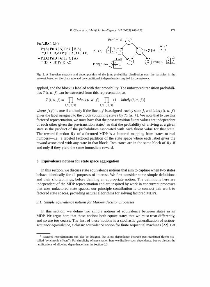
partition of X, where the labels are elements of Y . A conditional probability distributionPr(A|B) is a mapping from the domain of B to probability distributions over the domainof A, and so can be specified by giving a labeled partition—this is a factored conditionalprobability distribution. A joint probability distribution over a set of discrete variablescan be represented compactly by exploiting conditional independencies as a Bayesianbelief network [41]. Here, equivalent compactness is achieved as follows. First, the jointdistribution can be written as a product of conditional distributions using the chain rule (forany total ordering of the variables). Next, each of the conditional distributions involved canbe simplified by omitting any conditioning variables that are irrelevant due to conditionallyindependence. Finally, the simplified distributions are written in factored form. A jointdistribution so written is called a factored joint probability distribution. We show anexample of such a factored joint distribution in Fig. 2.
2.3.3. Factored Markov decision processesFactored MDPs can be represented using a variety of approaches, including Proba-
bilistic STRIPS Operators (PSOs) [20,21,29] and 2-stage Temporal Bayesian Networks(2TBNs) [13]. For details of these approaches, we refer to [8]. Here, we will use a rep-resentation, similar in spirit, but focusing on the state-space partitions involved. An MDPM = 〈Q,A,T ,R〉 can be given in factored form by giving a quadruple 〈F,A,TF ,RF 〉,6where the state space Q is given in factored form by the set of state variables F (withno constraining formula). The state-transition distribution of a factored MDP is specifiedby giving, for each fluent f and action α, a factored conditional probability distributionTF (α,f ) representing the probability that f is true after taking α, given the state in whichthe action is taken—TF (α,f ) is7 a partition of the state space, where two states are in thesame block if and only if they result in the same probability of setting f to true when α is
5 Various restrictions on the form of the formulas lead to various representations (e.g., decision trees).6 We discuss factored action spaces further in Section 6.1, and synchronic effects in Section 6.3.7 By our definition of “factored conditional probability distribution”.
R. Givan et al. / Artificial Intelligence 147 (2003) 163–223 171
Fig. 2. A Bayesian network and decomposition of the joint probability distribution over the variables in thenetwork based on the chain rule and the conditional independencies implied by the network.
applied, and the block is labeled with that probability. The unfactored transition probabili-ties T (i,α, j) can be extracted from this representation as
T (i,α, j)=∏
{f |j (f )}labelF (i, α,f )
∏{f |¬j (f )}
(1− labelF (i, α,f )
)where j (f ) is true if and only if the fluent f is assigned true by state j , and labelF (i, α,f )gives the label assigned to the block containing state i by TF (α,f ). We note that to use thisfactored representation, we must have that the post-transition fluent values are independentof each other given the pre-transition state,8 so that the probability of arriving at a givenstate is the product of the probabilities associated with each fluent value for that state.The reward function RF of a factored MDP is a factored mapping from states to realnumbers—i.e., a labeled factored partition of the state space where each label gives thereward associated with any state in that block. Two states are in the same block of RF ifand only if they yield the same immediate reward.
3. Equivalence notions for state space aggregation
In this section, we discuss state equivalence notions that aim to capture when two statesbehave identically for all purposes of interest. We first consider some simple definitionsand their shortcomings, before defining an appropriate notion. The definitions here areindependent of the MDP representation and are inspired by work in concurrent processesthat uses unfactored state spaces; our principle contribution is to connect this work tofactored state spaces, providing natural algorithms for solving factored MDPs.
3.1. Simple equivalence notions for Markov decision processes
In this section, we define two simple notions of equivalence between states in anMDP. We argue here that these notions both equate states that we must treat differently,and so are too coarse. The first of these notions is a stochastic generalization of action-sequence equivalence, a classic equivalence notion for finite sequential machines [22]. Let
8 Factored representations can also be designed that allow dependence between post-transition fluents (so-called “synchronic effects”). For simplicity of presentation here we disallow such dependence, but we discuss theramifications of allowing dependence later, in Section 6.3.
172 R. Givan et al. / Artificial Intelligence 147 (2003) 163–223
F = 〈Q,A,O,T ,R〉 and F ′ = 〈Q′,A,O,T ′,R′〉 be two FSMs over the same input and
output sets. The states i of F and j of F ′ are action-sequence equivalent if and only if forevery input sequence ξ , the same set of output sequences φ can be generated under ξ fromeither state i or state j , i.e.,∀ξ{φ | ξ →F,i φ} = {φ | ξ →F ′,j φ}.This equivalence notion also naturally applies to two states from the same FSM.
We now generalize this notion, for the stochastic case, to an equivalence notion betweenstates in MDPs. The distribution over reward sequences associated with a given MDPassigns to each sequence of actions α1, . . . , αk and starting state q a probability distributionover length k sequences of real values r1, . . . , rk . This distribution gives the probability ofobtaining the sequence of rewards r1, . . . , rk when starting from state q and performingaction sequence α1, . . . , αk . Let M = 〈Q,A,T ,R〉 and MDP M ′ = 〈Q′,A,T ′,R′〉 be twoMDPs with the same action space. The states i of M and j of M ′ are action-sequenceequivalent if and only if for every sequence of possible actions α1, . . . , αn, for any n, thedistributions over reward sequences for i in M and j in M ′ are the same. Note that thisdefinition applies naturally to two states within the same MDP as well.
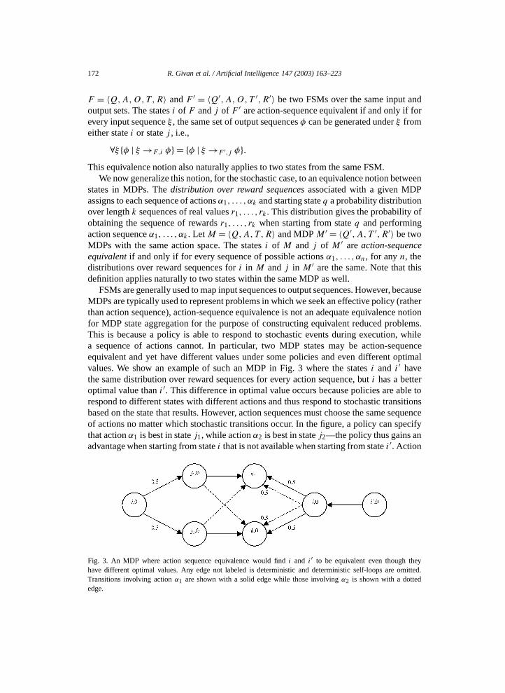
FSMs are generally used to map input sequences to output sequences. However, becauseMDPs are typically used to represent problems in which we seek an effective policy (ratherthan action sequence), action-sequence equivalence is not an adequate equivalence notionfor MDP state aggregation for the purpose of constructing equivalent reduced problems.This is because a policy is able to respond to stochastic events during execution, whilea sequence of actions cannot. In particular, two MDP states may be action-sequenceequivalent and yet have different values under some policies and even different optimalvalues. We show an example of such an MDP in Fig. 3 where the states i and i ′ havethe same distribution over reward sequences for every action sequence, but i has a betteroptimal value than i ′. This difference in optimal value occurs because policies are able torespond to different states with different actions and thus respond to stochastic transitionsbased on the state that results. However, action sequences must choose the same sequenceof actions no matter which stochastic transitions occur. In the figure, a policy can specifythat action α1 is best in state j1, while action α2 is best in state j2—the policy thus gains anadvantage when starting from state i that is not available when starting from state i ′. Action
Fig. 3. An MDP where action sequence equivalence would find i and i′ to be equivalent even though theyhave different optimal values. Any edge not labeled is deterministic and deterministic self-loops are omitted.Transitions involving action α1 are shown with a solid edge while those involving α2 is shown with a dottededge.
R. Givan et al. / Artificial Intelligence 147 (2003) 163–223 173
sequences, however, must commit to the entire sequence of actions that will be performed
at once and thus find states i and i ′ equally attractive.The failure of action-sequence equivalence to separate states with different optimalvalues suggests a second method for determining state equivalence: directly comparingthe optimal values of states. We call this notion optimal value equivalence. MDP states i
and j are optimal value equivalent if and only if they have the same optimal value.Optimal value equivalence also has substantial shortcomings. States equivalent to each
other under optimal value equivalence may have entirely different dynamics with respectto action choices. In general, an optimal policy differentiates such states. In some sense,the fact that the states share the same optimal value may be a “coincidence”. As a result,we have no means to calculate equivalence under this notion, short of computing andcomparing the optimal values of the states—but since an optimal policy can be found bygreedy one-step look-ahead from the optimal values, computing this equivalence relationwill be as hard as solving the original MDP. Furthermore, we are interested in aggregatingequivalent states in order to generate a reduced MDP. While the equivalence classes underoptimal value equivalence can serve as the state space for a reduced model, it is unclearwhat the effects of an action from such an aggregate state should be—the effects of a singleaction on different equivalent states might be entirely different. Even if we manage to finda way to adequately define the effects of the actions in this case, it is not clear how togeneralize a policy on a reduced model to the original MDP.
Neither of these equivalence relations suffices. However, the desired equivalencerelation will be a refinement of both of these: if two states are equivalent, they will beboth action sequence equivalent and optimal value equivalent. To see why, consider theproposed use for the equivalence notion, namely to aggregate states defining a smallerequivalent MDP that we can then solve in order to generalize that solution to the largeroriginal MDP. For the reduced MDP to be well defined, the reward value for all equivalentstates must be equal; likewise, the transition distributions for all equivalent states and anyaction must be equal (at the aggregate level). Thus, the desired equivalence relation shouldonly equate states that are both action sequence and optimal value equivalent (the formeris proved by induction on sequence length and the latter by induction on horizon).
3.2. Bisimulation for non-deterministic finite sequential machines
Bisimulation for FSM states captures more state properties than is possible using actionsequence equivalence. Bisimulation for concurrent processes [40] generalizes a similarconcept for deterministic FSM states from [22].
Let F = 〈Q,A,O,T ,R〉 and F ′ = 〈Q′,A,O,T ′,R′〉 be two FSMs over the same inputand output spaces. A relation E ⊆Q×Q′ is a bisimulation if each i ∈Q (and j ∈Q′) isin some pair in E, and whenever E(i, j) then the following hold for all actions α in A,
(1) R(i)=R′(j),(2) for i ′ in Q s.t. T (i,α, i ′), there is a j ′ in Q′ s.t. E(i ′, j ′) and T ′(j,α, j ′), and
conversely,(3) for j ′ in Q′ s.t. T ′(j,α, j ′), there is an i ′ in Q s.t. E(i ′, j ′) and T (i,α, i ′).
174 R. Givan et al. / Artificial Intelligence 147 (2003) 163–223
We say two FSM states i and j are bisimilar if there is some bisimulation B between their
FSMs in which B(i, j) holds. Bisimilarity is an equivalence relation, itself a bisimulation.The reflexive symmetric transitive closure of any bisimulation between two FSMs,restricted to the state space of either FSM gives an equivalence relation which partitionsthe state space of that FSM. The bisimulation can be thought of as a one-to-one mappingbetween the blocks of these two partitions (one for each FSM) where the two blocks arerelated if and only if some of their members are related. All block members are bisimilar toeach other and to all the states in the block related to that block by the bisimulation. Next,an immediate consequence of the theory of bisimulation [40].
Theorem 1. FSM states related by a bisimulation are action-sequence equivalent.9
We note that optimal-value equivalence is not defined for FSMs.Aggregation algorithms construct a partition of the state space Q and aggregate the
states in each partition block into a single state (creating one aggregate state per partitionblock) in order to create a smaller FSM with similar properties. When the partition used isdue to a bisimulation, the resulting aggregate states are action-sequence equivalent to thecorresponding states of the original FSM. The following theorem is a non-deterministicgeneralization of a similar theorem given in [22].
Theorem 2. Given an FSM F = 〈Q,A,O,T ,R〉 and an equivalence relation E ⊆Q×Q
that is a bisimulation, there is a unique quotient machine F/E and each state i in Q isbisimilar to the state i/E in F/E.10
Hennessy and Milner in [23] show that bisimulation captures exactly those propertiesof FSM states which can be described in Hennessy–Milner Modal Logic (HML).11 Webriefly define this logic here as an aside—we do not build on this aspect of bisimulationhere. The theorem below states that HML can express exactly those properties that can beused for state aggregation in the factored FSM methods we study. Following [30],12 theformulas ψ of HML are given by the syntax:
ψ ::= True | False | [α,o]ψ | 〈α,o〉ψ | (ψ1 ∨ψ2) | (ψ1 ∧ψ2).
The satisfaction relation i |= ψ between a state i in an FSM F and a HML formula ψ isdefined as usual for modal logics and Kripke models. Thus, i |= 〈α,o〉ψ whenever j |= ψ
for some j where T (i,α, j) and R(j) = o, and dually, i |= [α,o]ψ whenever T (i,α, j)and R(j)= o implies j |=ψ .
9 For space reasons, we do not repeat the proof of this result.10 For space reasons, we do not repeat the proof of this result.11 We note that the semantics of concurrent processes work deals with domains that are generally infinite and
possibly uncountable. Our presentation for FSMs is thus a specialization of that work to finite state spaces.12 HML and the corresponding bisimulation notion are normally defined for sequential machines with no
outputs, where the only issue is whether an action sequence is allowed or not. We make the simple generalizationto having outputs in order to ease the construction of the MDP analogy and to make the relationship between theliteratures more apparent.
R. Givan et al. / Artificial Intelligence 147 (2003) 163–223 175
Theorem 3 [23]. Two states i and j of an FSM F are bisimilar just in case they satisfy
exactly the same HML formulas.133.3. Stochastic bisimulation for Markov decision processes
In this section, we define stochastic bisimilarity for MDPs as a generalization ofbisimilarity for FSMs, generalizing “output” to “reward” and adding probabilities.Stochastic bisimilarity differs from bisimilarity in that transition behavior similarity mustbe measured at the equivalence class (or “block”) level—bisimilar states must have thesame block transition probabilities to each block of “similar” states.
The i/E notation generalizes to any relation E ⊆ Q × Q′. Define i/E be theequivalence class of i under the reflexive, symmetric, transitive closure of E, restrictedto Q, when i ∈Q (restrict to Q′ when i ∈Q′). The definitions are identical when E is anequivalence relation in Q×Q.
Let M = 〈Q,A,T ,R〉 and M ′ = 〈Q′,A,T ′,R′〉 be two MDPs with the same actionspace, and let E ⊆Q×Q′ be a relation. We say that E is a stochastic bisimulation14 ifeach i ∈Q (and j ∈ Q′) appears in some pair in E, and, whenever E(i, j), both of thefollowing hold for all actions α in A,
(1) R(i/E) and R′(j/E) are well defined and equal to each other.(2) For states i ′ in Q, and j ′ in Q′ s.t. E(i ′, j ′), T (i, α, i ′/E)= T ′(j,α, j ′/E).
See Section 2.2 for the definition of T (i,α,B) for a block B . We say that two MDP statesi and j are stochastically bisimilar if there is some stochastic bisimulation between theirMDPs which relates i and j . Note that these definitions can be applied naturally when thetwo MDPs are the same. This definition is closely related to the definition of probabilisticbisimulation for probabilistic transition systems (MDPs with no utility or reward specified)given in [30].
Theorem 4. Stochastic bisimilarity restricted to the states of a single MDP is anequivalence relation, and is itself a stochastic bisimulation from that MDP to itself.15
A stochastic bisimulation can be viewed as a bijection between corresponding blocksof partitions of the corresponding state spaces. So two MDPs will have a bisimulationbetween them exactly when there exist partitions of the two state spaces whose blockscan be put into a one-to-one correspondence preserving block transition probabilities and
13 For space reasons, we do not repeat the proof of this result.14 Stochastic bisimulation is also closely related to the substitution property of finite automata developed in
[22] and the notion of lumpability for Markov chains [27].15 We note that the proofs of all the theorems presented in this paper, except where omitted and explicitly noted,
are left until Appendix A for sake of readability.
176 R. Givan et al. / Artificial Intelligence 147 (2003) 163–223
rewards. Stochastic bisimulations that are equivalence relations have several desirable
properties as equivalence relations on MDP states.16Theorem 5. Any stochastic bisimulation that is an equivalence relation is a refinement ofboth optimal value equivalence and action sequence equivalence.
We are interested in state space aggregation and thus primarily in equivalence relations.The following theorem ensures that we can construct an equivalence relation from anybisimulation that is not already an equivalence relation.
Theorem 6. The reflexive, symmetric, transitive closure of any stochastic bisimulation fromMDP M = 〈Q,A,T ,R〉 to any MDP, restricted to Q × Q, is an equivalence relationE ⊆Q×Q that is a stochastic bisimulation from M to M .
Any stochastic bisimulation used for aggregation preserves the optimal value and actionsequence properties as well as the optimal policies of the model:
Theorem 7. Given an MDP M = 〈Q,A,T ,R〉 and an equivalence relation E ⊆Q×Q
that is a stochastic bisimulation, each state i in Q is stochastically bisimilar to the statei/E in M/E. Moreover, any optimal policy of M/E induces an optimal policy in theoriginal MDP.
It is possible to give a stochastic modal logic, similar to the Hennessy–Milner modallogic above, that captures those properties of MDP states that are discriminated bystochastic bisimilarity (e.g., see [30] which omits rewards).
4. Model minimization
Any stochastic bisimulation can be used to perform model reduction by aggregatingstates that are equivalent under that bisimulation. The definitions ensure that there arenatural meanings for the actions on the aggregate states. The coarsest bisimulation(stochastic bisimilarity) gives the smallest model, which we call the “minimal model” ofthe original MDP. In this section, we investigate how to find bisimulations, and bisimilarityefficiently. We first summarize previous work on computing bisimilarity in FSM models,and then generalize this work to our domain of MDPs.
4.1. Minimizing finite state machines with bisimilarity
Concurrent process theory provides methods for computing the bisimilarity relation onan FSM state space. We summarize one method, and show how to use it to compute a
16 It is possible to give a stochastic modal logic for those properties of MDP states that are discriminated bystochastic bisimilarity. For an example of a closely related logic that achieves this goal for probabilistic transitionsystems, see the probabilistic modal logic given in [30].
R. Givan et al. / Artificial Intelligence 147 (2003) 163–223 177
minimal FSM equivalent to the original [38]. Consider FSMs F = 〈Q,A,O,T ,R〉 and
F ′ = 〈Q′,A,O ′, T ′,R′〉 and binary relation E ⊆Q×Q′. Define H(E) to be the set of allpairs (i, j ) from Q×Q′ satisfying the following two properties. First, E(i , j) must hold.Second, for every action α ∈A, each of the following conditions holds:(1) R(i)=R′(j),(2) for i ′ in Q s.t. T (i,α, i ′), there is a j ′ in Q′ s.t. E(i ′, j ′) and T ′(j,α, j ′), and
conversely,(3) for j ′ in Q′ s.t. T ′(j,α, j ′), there is an i ′ in Q s.t. E(i ′, j ′) and T (i,α, i ′).
We note that H(E) is formed by removing pairs from E that violate the bisimulationconstraints relative to E. We can then define a sequence of relations E0,E1, . . . by takingE0 =Q×Q and Ex+1 =H(Ex). Since E(i, j) is required for (i, j ) to be in H(E), it isapparent that this sequence will be monotone decreasing, i.e., Ex+1 ⊆ Ex . It also followsthat any fixed-point of H is a bisimulation between F and itself. Therefore, by iterating H
on an initial (finite) E =Q×Q we eventually find a fixed-point (which is therefore alsoa bisimulation). By Theorem 2, this bisimulation can be used in state space aggregationto produce a quotient model with states that are action sequence equivalent to the originalmodel.
Further analysis has demonstrated that the resulting bisimulation contains every otherbisimulation, and is thus the largest17 bisimulation between F and itself [38]. As a result,this bisimulation is the bisimilarity relation on Q, and produces the smallest quotient modelof any bisimulation when used in state space aggregation.
4.2. Minimizing Markov decision processes with stochastic bisimilarity
We show here how the direct generalization of the techniques described above forcomputing bisimilarity yields an algorithm for computing stochastic bisimilarity that inturn is the basis for a model minimization algorithm. Given an MDP M = 〈Q,A,T ,R〉,we define an operator I on binary relations E ⊆Q×Q similar to H . Let I (E) to be theset of all pairs i, j such that E(i, j),R(i)=R(j), and for every action α in A and state i ′in Q,
T (i,α, i ′/E)= T (j,α, i ′/E).
We can again define a decreasing sequence of equivalence relations E0 ⊇ E1 ⊇ · · · bytaking E0 =Q×Q and Ex+1 = I (Ex). Again, the definitions immediately imply that anyfixed point of I is a stochastic bisimulation between M and itself. Therefore, by iterating I
on an initial (finite) E =Q×Q, we are guaranteed to eventually find a fixed point (whichis therefore a stochastic bisimulation). Theorem 7 implies that this stochastic bisimulationcan be used in state space aggregation to produce a quotient model containing blocks thatare both action sequence and optimal value equivalent to the original model.
The resulting stochastic bisimulation contains every other stochastic bisimulationbetween M and itself, and is thus the largest stochastic bisimulation between M and
17 Here, by “largest”, we are viewing relations as sets of pairs partially ordered by subset.
178 R. Givan et al. / Artificial Intelligence 147 (2003) 163–223
itself,18 the stochastic bisimilarity relation on Q. Aggregation using this relation gives
a coarser (smaller) aggregate reduced model than with any other bisimulation. Useof this technique for computing bisimilarity for state space aggregation and modelreduction provides a straightforward motivation for and derivation of a model minimizationalgorithm: simply aggregate bisimilar states to form the coarsest equivalent model, thequotient model under bisimilarity.4.3. Implementing model minimization using block splitting
We now describe a method for computing stochastic bisimilarity19 by repeatedlysplitting the state space into smaller and smaller blocks, much like the I (E) operationdescribed above. We start by introducing a desired property for partition blocks that can bechecked locally (between two blocks) but that when present globally (between all pairs ofblocks) ensures that a bisimulation has been found.
We say that a block B is stable with respect to block C if and only if every state p in B
has the same probability T (p,α,C) of being carried into block C for every action α andthe block reward R(B) is well defined. We say that B is stable with respect to equivalencerelation E if B is stable with respect to every block in the partition induced by E. We saythat an equivalence relation E is stable if every block in the induced partition is stable withrespect to E. These definitions immediately imply that any stable equivalence relation is abisimulation.
The equivalence relation I (E) can be defined in terms of stability as the relation inducedby the coarsest partition (among those refining E) containing only blocks that are stablewith respect to E. This partition can be found by splitting each block of E into maximalsub-blocks that are stable with respect to E (i.e., stable with respect to each block of E).To make this concrete, we define a split operation that enforces this stability property for aparticular pair of blocks.
Let P be a partition of Q, B a block in P , and C a set of states C ⊂Q. We define a newpartition denoted SPLIT(B,C,P ) by replacing B with the uniquely determined sub-blocks{B1, . . . ,Bk} such that each Bi is a maximal sub-block of B that is stable with respect toC. Since Bi is stable with respect to C, for any action α and for states p and q from thesame block Bi we have that
T (p,α,C)= T (q,α,C) and R(p)=R(q).
Since the Bi are maximal, for states p and q from different blocks, either
T (p,α,C) �= T (q,α,C) or R(p) �=R(q).
The SPLIT operation can be used to compute I (E) by repeated splitting of the blocksof the partition induced by E as follows:
18 We can show that if E contains a bisimulation B, then I (E) must still contain that bisimulation—the keystep is to show that T (i,α, i′/E)= T (j,α, i′/E) for any i′ in Q, any α in A, and any i and j such that B(i, j).
19 Our algorithm is a stochastic adaptation of an algorithm in [31] that is related to an algorithm by [3]. All ofthese algorithms derive naturally from the known properties of bisimilarity in concurrent process theory [38].
R. Givan et al. / Artificial Intelligence 147 (2003) 163–223 179
Let P ′ = P = the partition induced by E
For each block C in P
While P ′ contains a block B for which P ′ �= SPLIT(B,C,P ′)P ′ = SPLIT(B,C,P ′) /* blocks added here are
stable wrt. C */
/* so need not be checked in While test */
I (E)= the equivalence relation represented by P ′
We refer to this algorithm as the partition improvement algorithm, and to iterativelyapplying partition improvement starting with {Q} as partition iteration. However, inpartition iteration, suppose a block B has been split so that P ′ contains sub-blocksB1, . . . ,Bk of B . Now, splitting other blocks C to create stability with respect to B is nolonger necessary since, we will be splitting C to create stability with respect to B1, . . . ,Bk
in a later iteration of I . Blocks that are stable with respect to B1, . . . ,Bk are necessarilystable with respect to B . This analysis leads to the following simpler algorithm, whichbypasses computing I iteratively and computes the greatest fixed point of I more directly:
Let P = {Q} /* trivial one block partition */
While P contains block B &C s.t. P �= SPLIT(B,C,P )
P = SPLIT(B,C,P)
Greatest Fixed point of I = the equivalence relation
given by P
We refer to this algorithm as the model minimization algorithm, and we refer to theP �= SPLIT(B,C,P ) check as the stability check for blocks B and C. That modelminimization computes a fixed point of I follows from the fact that when all blocks ofa partition are stable with respect to that partition, the partition is a bisimulation (andthus a fixed point of I ). The following lemma and corollary then imply that either modelminimization or partition iteration can be used to compute the greatest fixed point of I .
Lemma 8.1. Given equivalence relation E on Q and states p and q such that T (p,α,C) �=T (q,α,C) for some action α and block C of E,p and q are not related by any stochasticbisimulation refining E.
Corollary 8.2. Let E be an equivalence relation on Q,B a block in E, and C a unionof blocks from E. Every bisimulation on Q that refines E is a refinement of the partitionSPLIT(B,C,E).
Theorem 8. Partition iteration and model minimization both compute stochastic bisimilar-ity.
By repeatedly finding unstable blocks and splitting them, we can thus find thebisimilarity partition in linearly many splits relative to the final partition size (each splitincreases the partition size, which cannot exceed that of the bisimilarity partition, so
180 R. Givan et al. / Artificial Intelligence 147 (2003) 163–223
there are at most linearly many splits). The model minimization algorithm performs at
most quadratically many stability checks:20 simply check each pair of blocks for stability,splitting each unstable block as it is discovered. The cost of each split operation and eachstability check depends heavily on the partition representation and is discussed in detaillater in this paper.We note that this analysis implies that the partition computed by model minimizationis the stochastic bisimilarity partition, regardless of which block is selected for splitting ateach iteration of the While loop. We therefore leave this choice unspecified.
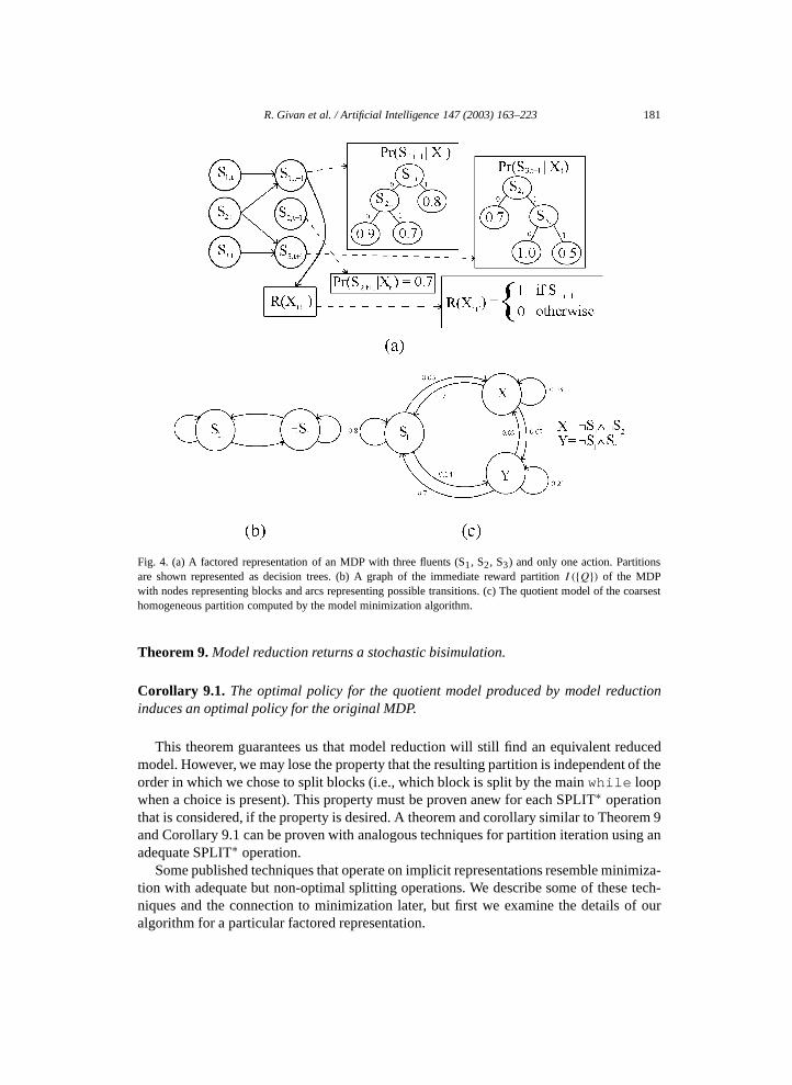
Fig. 4(a) shows an MDP in factored representation by giving a DBN with the conditionalprobability tables represented as decision trees, using the representation developed in [9,13]. Fig. 4(b) shows the immediate-reward partition for this MDP, which is computed byI ({Q}). There are two blocks in this partition: states in which the reward is one and statesin which the reward is zero. Fig. 4(c) shows the quotient model for the refined partitionconstructed by the model minimization algorithm. Aggregate states (blocks of the twopartitions) are described as formulas involving fluents, e.g., ¬S1 ∧ S2 is the set of statesin which S1 is false and S2 is true. A factored SPLIT operation suitable for finding thisquotient model without enumerating the underlying state space is described in Section 4.4.
The model-minimization algorithm is given independently of the underlying representa-tion for state-space partitions. However, in order for the algorithm to guarantee finding thetarget partition, we must have a partition representation sufficiently expressive to representan arbitrary partition of the state space. Such partition representations may be expensiveto manipulate, and may blow up in size. For this reason, partition manipulation opera-tions that do not exactly implement the splitting operation described above can still be ofuse—typically these splitting operations guarantee that the resulting partition can be repre-sented in a more restrictive partition representation. Such operations can still be adequatefor our purposes if, whenever a split is requested, the operation splits “at least as much” asrequested.
Formally, we say that a block splitting operation SPLIT∗ is adequate if SPLIT∗(B,C,P )
is always a refinement of SPLIT(B,C,P ). Adequate split operations that can return par-titions that are strictly finer than SPLIT are said to be non-optimal. The minimizationalgorithm, with SPLIT replaced by an adequate SPLIT∗, is a model reduction algorithm.Note that non-optimal SPLIT∗ operations may be cheaper to implement than SPLIT, eventhough they “split more” than SPLIT. One natural way to define an adequate but non-optimal SPLIT∗ operation is to base the definition on a partition representation that canrepresent only some possible partitions. In this case, SPLIT∗ is defined as a coarsest repre-sentable refinement of the optimal partition computed by SPLIT. (For many natural repre-sentations, e.g., fluentwise partitions, this coarsest refinement is unique.) As shown by thefollowing theorem, the model reduction algorithm remains sound.
20 Observe that the stability of a block C with respect to another block B and any action is not affected bysplitting blocks other than B and C , so no pair of blocks need to be checked for stability more than once for eachaction. Also the number of blocks ever considered cannot exceed twice the number of blocks in the final partition,since blocks that are split can be viewed as internal nodes of a tree. Here, the root of the tree is the block of allstates, the leaves of the tree are the blocks of the final partition, and the children of any node are the blocks thatresult from splitting the block at the node. These facts imply the quadratic bound on stability checks.
R. Givan et al. / Artificial Intelligence 147 (2003) 163–223 181
Fig. 4. (a) A factored representation of an MDP with three fluents (S1, S2, S3) and only one action. Partitionsare shown represented as decision trees. (b) A graph of the immediate reward partition I ({Q}) of the MDPwith nodes representing blocks and arcs representing possible transitions. (c) The quotient model of the coarsesthomogeneous partition computed by the model minimization algorithm.
Theorem 9. Model reduction returns a stochastic bisimulation.
Corollary 9.1. The optimal policy for the quotient model produced by model reductioninduces an optimal policy for the original MDP.
This theorem guarantees us that model reduction will still find an equivalent reducedmodel. However, we may lose the property that the resulting partition is independent of theorder in which we chose to split blocks (i.e., which block is split by the main while loopwhen a choice is present). This property must be proven anew for each SPLIT∗ operationthat is considered, if the property is desired. A theorem and corollary similar to Theorem 9and Corollary 9.1 can be proven with analogous techniques for partition iteration using anadequate SPLIT∗ operation.
Some published techniques that operate on implicit representations resemble minimiza-tion with adequate but non-optimal splitting operations. We describe some of these tech-niques and the connection to minimization later, but first we examine the details of ouralgorithm for a particular factored representation.
182 R. Givan et al. / Artificial Intelligence 147 (2003) 163–223
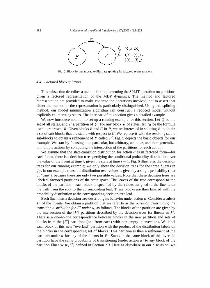
Fig. 5. Block formulas used to illustrate splitting for factored representations.
4.4. Factored block splitting
This subsection describes a method for implementing the SPLIT operation on partitionsgiven a factored representation of the MDP dynamics. The method and factoredrepresentation are provided to make concrete the operations involved, not to assert thateither the method or the representation is particularly distinguished. Using this splittingmethod, our model minimization algorithm can construct a reduced model withoutexplicitly enumerating states. The later part of this section gives a detailed example.
We now introduce notation to set up a running example for this section. Let Q be theset of all states, and P a partition of Q. For any block B of states, let fB be the formulaused to represent B . Given blocks B and C in P , we are interested in splitting B to obtaina set of sub-blocks that are stable with respect to C. We replace B with the resulting stablesub-blocks to obtain a refinement of P called P ′. Fig. 5 depicts the basic objects for ourexample. We start by focusing on a particular, but arbitrary, action α, and then generalizeto multiple actions by computing the intersection of the partitions for each action.
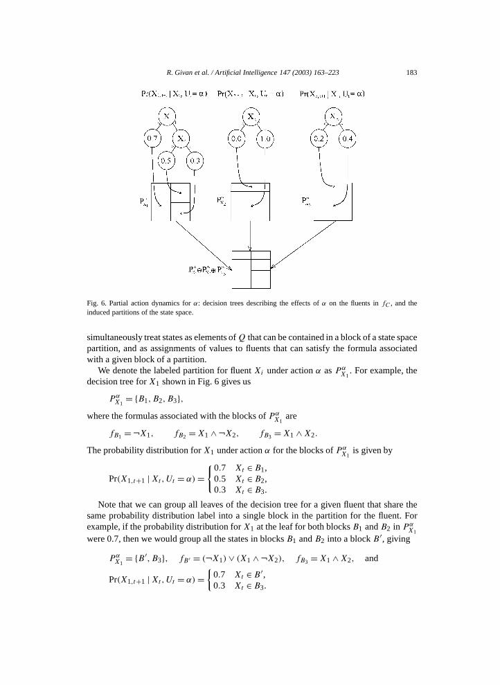
We assume that the state-transition distribution for action α is in factored form—foreach fluent, there is a decision tree specifying the conditional probability distribution overthe value of the fluent at time t , given the state at time t − 1. Fig. 6 illustrates the decisiontrees for our running example; we only show the decision trees for the three fluents infC . In our example trees, the distribution over values is given by a single probability (thatof “true”), because there are only two possible values. Note that these decision trees arelabeled, factored partitions of the state space. The leaves of the tree correspond to theblocks of the partition—each block is specified by the values assigned to the fluents onthe path from the root to the corresponding leaf. These blocks are then labeled with theprobability distribution at the corresponding decision-tree leaf.
Each fluent has a decision tree describing its behavior under action α. Consider a subsetF ′ of the fluents. We obtain a partition that we refer to as the partition determining thetransition distribution for F ′ under α, as follows. The blocks of the partition are given bythe intersection of the |F ′| partitions described by the decision trees for fluents in F ′.There is a one-to-one correspondence between blocks in the new partition and sets ofblocks from the |F ′| partitions (one from each) with non-empty intersections. We labeleach block of this new “overlaid” partition with the product of the distribution labels onthe blocks in the corresponding set of blocks. This partition is then a refinement of thepartition under α for any of the fluents in F ′. States in the same block of this overlaidpartition have the same probability of transitioning (under action α) to any block of thepartition Fluentwise(F ′) defined in Section 2.3. Here as elsewhere in our discussion, we
R. Givan et al. / Artificial Intelligence 147 (2003) 163–223 183
Fig. 6. Partial action dynamics for α: decision trees describing the effects of α on the fluents in fC , and theinduced partitions of the state space.
simultaneously treat states as elements of Q that can be contained in a block of a state spacepartition, and as assignments of values to fluents that can satisfy the formula associatedwith a given block of a partition.
We denote the labeled partition for fluent Xi under action α as PαX1
. For example, thedecision tree for X1 shown in Fig. 6 gives us
PαX1= {B1,B2,B3},
where the formulas associated with the blocks of PαX1
are
fB1 =¬X1, fB2 =X1 ∧¬X2, fB3 =X1 ∧X2.
The probability distribution for X1 under action α for the blocks of PαX1
is given by
Pr(X1,t+1 |Xt,Ut = α)={0.7 Xt ∈B1,
0.5 Xt ∈B2,0.3 Xt ∈B3.
Note that we can group all leaves of the decision tree for a given fluent that share thesame probability distribution label into a single block in the partition for the fluent. Forexample, if the probability distribution for X1 at the leaf for both blocks B1 and B2 in Pα
X1
were 0.7, then we would group all the states in blocks B1 and B2 into a block B ′, giving
PαX1= {B ′,B3}, fB ′ = (¬X1)∨ (X1 ∧¬X2), fB3 =X1 ∧X2, and
Pr(X1,t+1 |Xt,Ut = α)={
0.7 Xt ∈B ′,0.3 Xt ∈B3.
184 R. Givan et al. / Artificial Intelligence 147 (2003) 163–223
For each fluent Xi , the partition Pα groups states that behave the same under action
Xiα with regards to Xi . However, what we want is to group states in B that behave thesame under action α with respect to C. Since C is specified using a formula fC , we needonly concern ourselves with fluents mentioned in fC , as the other fluents do not influencewhether or not we end up in C. If we take the intersection of all the partitions for each ofthe fluents mentioned in fC , we obtain the coarsest partition that is a refinement of all thosefluent partitions. This partition distinguishes between states with different probabilities ofending up in C. We can then restrict the partition to the block B to obtain the sub-blocksof B where states in the same sub-block all have the same probability of ending up in C
after taking action α. Therefore, if Fluents(fC ) is the set of all fluents appearing in fC ,the partition determining the transition distribution for Fluents(fC) under α makes all thenecessary state distinctions.
The procedure Block-split( ) shown in Fig. 7 computes the coarsest partition of B thatis a refinement of all the partitions associated with the fluents in fC and the action α. Itdoes so by first computing the coarsest partition of Q, which we will denote PQ, with thisproperty, and then intersecting each block in this partition with B . (In terms of representingblocks as formulas, intersection is just conjunction.) Applying this to our ongoing examplegives the following partitions:
PαX1= {X1 ∧X2,X1 ∧¬X2,¬X1}, P α
X2= {X3,¬X3}, P α
X3= {X3,¬X3},
PQ = {X1 ∧X2 ∧X3, X1 ∧X2 ∧¬X3, X1 ∧¬X2 ∧X3, X1 ∧¬X2 ∧¬X3,
¬X1 ∧X3, ¬X1 ∧¬X3}.Intersecting each block of PQ with fB (eliminating empty blocks) computes the finalpartition of B given by
{X1 ∧¬X2 ∧X3 ∧X4, X1 ∧¬X2 ∧¬X3 ∧X4,
¬X1 ∧¬X2 ∧X3 ∧X4, ¬X1 ∧¬X2 ∧¬X3 ∧X4}.This procedure runs, in the worst case, in time exponential in the number of fluentsmentioned in fC .21 As with most factored MDP algorithms, in the worst case, the factoringgains us no computational advantage.
One adequate but non-optimal splitting operation that works on the factored represen-tation is defined in terms of the procedure Block-split( ) as
SPLIT∗(B,C,P )= (P − {B})∪( ⋂
α∈ABlock-split(B,C,α)
).
We refer to SPLIT∗ defined in this manner as S-SPLIT, abbreviation “structure-basedsplitting”. Structure-based splitting the exact transition probabilities assigned to blocks ofstates. This splitting method splits two states if there is any way of setting the quantifyingparameters that would require splitting the states. S-SPLIT is non-optimal because it cannot
21 The order in which the fluents are handled can dramatically affect the run time of Partition-determining( ) ifinconsistent formulas are identified and eliminated on each recursive call.

R. Givan et al. / Artificial Intelligence 147 (2003) 163–223 185
Block-split(B,C,α)
return{fB ∧ f ∧ fR | f ∈ Partition-determining (Fluents(fC),α),fR ∈ Reward partition,and fB ∧ f ∧ fR is satisfiable };
Partition-determining(F,α) /* the partition determining thefluents in F */
if F = ∅ then return {true};for some X ∈ F,return {f ∧ fB ′ | B ′ ∈ Pα
X,
f ∈ Partition-determining (F − {X}, α), andf ∧ fB ′ is satisfiable};
Fig. 7. Procedure for partitioning block B with respect to block C and action α.
exploit “coincidences” in the quantifying parameters to aggregate “structurally” differentstates.
In order to implement an optimal split, we need to do a little more work. Specifically, wehave to combine blocks of Block-split(B,C,α) that have the same probability of endingup in C. Situations where we must combine such blocks in order to be optimal arisewhen an action, taken in different states from B , affects the fluents in fC differently, but“coincidentally” has the same overall probability of ending up in block C from the differentsource states. For example, suppose action α, taken in state p in B , has a 0.5 probabilityof setting fluent X1, and always sets fluent X2; however, when α is taken in state q inB , it has a 0.5 probability of setting fluent X2, and always sets fluent X1. If block C hasformula X1 ∧X2 both state p and state q have a 0.5 probability of transitioning to block C
under action α. However, p and q must be in separate blocks for each of the fluents in theformula X1∧X2, since α affects both X1 and X2 differently at p than at q—hence, Block-split( ) will partition p and q into different blocks, even though they behave the same withrespect to C. To compute the coarsening of Block-split(B,C,α) required to obtain optimalsplitting, we first consider a particular partition of the block C.
The partition of C that we use in computing an optimal split of B is the fluentwise22
partition Fluentwise(Fluents(C)), restricted to C. This partition has a block for eachassignment to the fluents in Fluents(C) consistent with fC . We denote this partitionas Fluentwise(C). In our example, fC = (X1 ∧ X2) ∨ (X2 ∧ X3) so Fluentwise(C) ={X1 ∧X2 ∧X3, X1 ∧X2 ∧ ¬X3, ¬X1 ∧X2 ∧X3} which we shall call C1,C2, and C3,respectively.
The probability of transition from Bj ∈ Block-split(B,C,α) to Ci ∈ Fluentwise(C) isdefined as
Pr(Xt+1 ∈ Cj |Xt ∈Bi,Ut = α)= Pr(Xt+1 ∈Cj |Xt = p,Ut = α),
22 See Section 2.3.
186 R. Givan et al. / Artificial Intelligence 147 (2003) 163–223
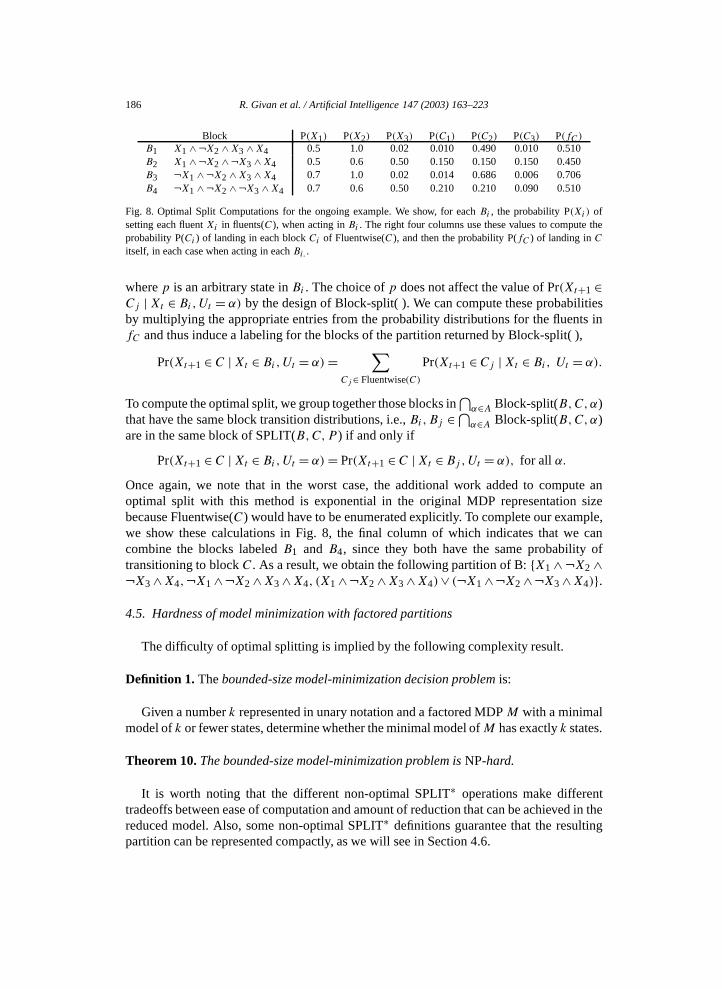
Block P(X1) P(X2) P(X3) P(C1) P(C2) P(C3) P(fC)
B1 X1 ∧¬X2 ∧X3 ∧X4 0.5 1.0 0.02 0.010 0.490 0.010 0.510B2 X1 ∧¬X2 ∧¬X3 ∧X4 0.5 0.6 0.50 0.150 0.150 0.150 0.450B3 ¬X1 ∧¬X2 ∧X3 ∧X4 0.7 1.0 0.02 0.014 0.686 0.006 0.706B4 ¬X1 ∧¬X2 ∧¬X3 ∧X4 0.7 0.6 0.50 0.210 0.210 0.090 0.510Fig. 8. Optimal Split Computations for the ongoing example. We show, for each Bi , the probability P(Xi) ofsetting each fluent Xi in fluents(C), when acting in Bi . The right four columns use these values to compute theprobability P(Ci ) of landing in each block Ci of Fluentwise(C), and then the probability P(fC ) of landing in C
itself, in each case when acting in each Bi. .
where p is an arbitrary state in Bi . The choice of p does not affect the value of Pr(Xt+1 ∈Cj |Xt ∈ Bi,Ut = α) by the design of Block-split( ). We can compute these probabilitiesby multiplying the appropriate entries from the probability distributions for the fluents infC and thus induce a labeling for the blocks of the partition returned by Block-split( ),
Pr(Xt+1 ∈ C |Xt ∈ Bi,Ut = α)=∑
Cj∈ Fluentwise(C)
Pr(Xt+1 ∈Cj |Xt ∈ Bi, Ut = α).
To compute the optimal split, we group together those blocks in⋂
α∈A Block-split(B,C,α)that have the same block transition distributions, i.e., Bi,Bj ∈⋂
α∈A Block-split(B,C,α)are in the same block of SPLIT(B,C,P ) if and only if
Pr(Xt+1 ∈ C |Xt ∈ Bi,Ut = α)= Pr(Xt+1 ∈C |Xt ∈Bj ,Ut = α), for all α.
Once again, we note that in the worst case, the additional work added to compute anoptimal split with this method is exponential in the original MDP representation sizebecause Fluentwise(C) would have to be enumerated explicitly. To complete our example,we show these calculations in Fig. 8, the final column of which indicates that we cancombine the blocks labeled B1 and B4, since they both have the same probability oftransitioning to block C. As a result, we obtain the following partition of B: {X1 ∧¬X2 ∧¬X3 ∧X4,¬X1 ∧¬X2 ∧X3 ∧X4, (X1 ∧¬X2 ∧X3 ∧X4)∨ (¬X1 ∧¬X2 ∧¬X3 ∧X4)}.
4.5. Hardness of model minimization with factored partitions
The difficulty of optimal splitting is implied by the following complexity result.
Definition 1. The bounded-size model-minimization decision problem is:
Given a number k represented in unary notation and a factored MDP M with a minimalmodel of k or fewer states, determine whether the minimal model of M has exactly k states.
Theorem 10. The bounded-size model-minimization problem is NP-hard.
It is worth noting that the different non-optimal SPLIT∗ operations make differenttradeoffs between ease of computation and amount of reduction that can be achieved in thereduced model. Also, some non-optimal SPLIT∗ definitions guarantee that the resultingpartition can be represented compactly, as we will see in Section 4.6.
R. Givan et al. / Artificial Intelligence 147 (2003) 163–223 187
Theorem 10 shows that model minimization will be expensive in the worst case,
regardless of how it is computed, even when small models exist. In addition, since ouroriginal algorithm presentation in [12] it has been shown that the factored-stability testrequired for the particular algorithm we present (and implicit in computing SPLIT) is alsoquite expensive to compute, being coNPC=P-hard [19].23 This result does not directlyimply hardness for the bounded-size model minimization problem (i.e., Theorem 10),because there could be other algorithms for addressing that problem without using SPLIT.4.6. Non-optimal block splitting for improved effectiveness
We discuss three different non-optimal block splitting approaches and the interactionbetween these approaches and our choice of partition representation as well as theconsequent improvement in effectiveness. The optimal SPLIT defined above requires ageneral-purpose partition representation to represent the partitions encountered duringmodel reduction—e.g., the DNF representation discussed in Section 2.3. Each of thealternative non-optimal SPLIT∗ approaches can guarantee that the resulting partition isrepresentable with a less expressive but more compact representation, as discussed below.
We motivate our non-optimal splitting approaches by noting that the optimal factoredSPLIT operation described in Section 4.4 has two phases, each of which can independentlytake time exponential in the input size. The first phase computes Block-split(B,C,α)for each action α, and uses it to refine B , defining the partition S-SPLIT(B,C,P ). Thesecond phase coarsens this partition, aggregating blocks that are “coincidentally” alike forthe particular quantifying parameters (transition probabilities and rewards) in the model.Our non-optimal splitting methods address each of these exponential phases, allowingpolynomial-time computation of the partition resulting from that phase.
The first non-optimal approach we discuss guarantees a fluentwise-representablepartition—recall from Section 2.3 that a fluentwise partition can be represented as a subsetof the fluents where the blocks of the partition correspond to the distinct truth assignmentsto that subset of fluents. We define the “fluentwise split” F-SPLIT(B,C,P ) to be thecoarsest refinement of SPLIT(B,C,P ) that is fluentwise representable. F-SPLIT(B,C,P )is the fluentwise partition described by the set of all fluents X such that there are twostates differing only on X that fall in different blocks of SPLIT(B,C,P ). Equivalently,F-SPLIT(B,C,P ) is the fluentwise partition described by the set of all fluents X thatare present in every DNF description of SPLIT(B,C,P ). As with SPLIT(B,C,P ), thefunction F-SPLIT(B,C,P ) can be computed in two phases. The first phase intersectspartitions from the action definitions, returning the coarsest fluentwise refinement of theresult. The second phase combines blocks in the resulting partition (due to “coincidences”),and again takes the coarsest fluentwise refinement, to yield the desired partition. The firstphase can be carried out efficiently in polynomial time in the size of the output, but thesecond phase appears to require time possibly exponential in its output size, because itappears to require enumerating the blocks of the first-phase output.
23 Goldsmith and Sloan in [19] also show that the complexity of performing a test for an approximate versionof stability, ε-stability, for an arbitrary partition is coNPPP-complete. (ε-stability, is a relaxed form of stabilitydefined in [14].)
188 R. Givan et al. / Artificial Intelligence 147 (2003) 163–223
To avoid the exponential time required in the second phase to detect “coincidences”
that depend on the quantifying parameters, we need to define a “structural” notion of blockstability—one that ignores the quantifying parameters. Because our factored representationdefines transition probabilities one fluent at a time, we will define structural stability in asimilar fluentwise manner.We say that a block B of a partition P is fluentwise stable with respect to fluent Xif and only if for every action α,B is a subset of some block of the partition TF (α,X).The block B is termed fluentwise stable with respect to block C if B is fluentwise stablewith respect to every fluent mentioned in every DNF formula describing block C. Wecall a partition P fluentwise stable if every block in the partition is fluentwise stable withrespect to every other block in the partition. It is straightforward to show that the “structuralsplit” S-SPLIT(B,C,P ), as defined above in Section 4.4, is the coarsest refinement ofSPLIT(B,C,P ) for which each sub-block of B is fluentwise stable with respect to C.
The operation S-SPLIT is adequate and is computed using Block-split( ) for each action,as described in Section 4.4, assuming that each block formula in the input partitionrepresentation is simplified (in the sense that any fluent mentioned must be mentionedto represent the block). This assumption holds for blocks represented as conjunctions ofliterals, as in decision-tree partitions. Under this assumption S-SPLIT can be computed intime polynomial in the size of its input formulas plus the number of new blocks introduced(which may be exponential in the input size). Analysis of S-SPLIT guarantees that ifeach input block is describable by a conjunction of literals then so are the blocks of theoutput partition, ensuring that the inputs are conjunctions of literals, if each partition in theoriginal factored MDP definition is so represented (e.g., if decision tree partitions are usedto define the MDP24), as long as all block splitting is done with S-SPLIT. This guaranteeallows model reduction with S-SPLIT to use this simpler representation of partitions. WithS-SPLIT the result of reduction is also not order-dependent, unlike some adequate, non-optimal splits (see Section 4.3).
Theorem 11. Given a partition P , there is a unique coarsest fluentwise-stable stochasticbisimulation refining P . Iterating S-SPLIT using model reduction or partition iterationstarting from P computes this bisimulation regardless of the order of block splitting.
To avoid exponential model-reduction time even when the resulting model is expo-nentially large, we can combine the above two concepts. We call the resulting “flu-entwise structural” split FS-SPLIT(B,C,P ). FS-SPLIT(B,C,P ) computes the coarsestfluentwise-representable refinement of SPLIT(B,C,P ) such that each sub-block of B isfluentwise stable with respect to C. The split operation FS-SPLIT is adequate and com-putable in time polynomial in the size of M , even for factoredM , and the resulting partitionis again independent of the order of splitting.
24 It is worth noting that decisions trees as used in this paper are less expressive than the disjoint conjunctionsof literals representation. That is to say there exist sets of disjoint conjunctions of literals that represent partitionsnot representable with decision trees, e.g., {A∧¬B,B ∧¬C,C ∧¬A,A∧B ∧C,¬A∧¬B ∧¬C}.
R. Givan et al. / Artificial Intelligence 147 (2003) 163–223 189
Theorem 12. Given a partition P , there is a unique coarsest stochastic bisimulation
refining P even under the restriction that the partition be both fluentwise stable andfluentwise representable. Iterating FS-SPLIT using model reduction or partition iterationstarting from P computes this bisimulation regardless of the order of block splitting.A variant of S-SPLIT that is closer to the optimal SPLIT can be derived by observingthat there is no need to split a block B to achieve fluentwise stability relative to adestination block C when the block B has a zero probability of transitioning to theblock C. This refinement does not affect FS-SPLIT due to the bias towards splitting ofthe “fluentwise” partition representation used, but adding this refinement does changeS-SPLIT. The resulting split operation, which we call R-SPLIT, is significant in that itis implicit in the previously published factored MDP algorithms in [9].
We define the regression region for a block B to be the block containing those states isuch that T (i,α,B) is non-zero. A block B is said to be regression stable with respect toblock C if B is either entirely contained in the regression region of C and B is fluentwisestable with respect to C or B does not overlap the regression region of C. The “regression”splitting operation R-SPLIT(B,C,P ) is the coarsest refinement of SPLIT(B,C,P ) suchthat each sub-block of B is regression stable with respect to C. We say a partition P isregression stable if every block of P is regression stable with respect to every other blockof P . R-SPLIT can be calculated using a modification of the Block-split function, givenin Fig. 7. For each action α, replacing the call Partition-determining(Fluents(C), α) withthe call Regression-determining(fC, α), invoking the pseudo-code shown in Fig. 9. Wenote that R-SPLIT, unlike S-SPLIT, depends on the specific transition probabilities (i.e.,whether each is zero or not), not just the partitions used in defining T . Given a partition(and factored MDP) using only blocks described by conjunctions of literals, IR-SPLITreturns another such partition.25 Unlike S-SPLIT, we do not have a method for computingR-SPLIT in worst-case polynomial-time in the number of blocks in the output partition(similarly, the corresponding algorithms in [9], as discussed below in Section 5, are notpolynomial in the output size).
Theorem 13. Given a partition P , there exists a unique coarsest regression-stablestochastic bisimulation refining P .
It turns out that this target partition can be computed by iterating R-SPLIT, as expected,but that the partition found may depend on the order in which splitting is done unless werestrict the starting partition representation, as follows.
Theorem 14. Let M be a factored MDP with all partition blocks represented asconjunctions of literals. Given a starting partition P also so represented, iteratingR-SPLIT using partition iteration computes the coarsest regression-stable stochasticbisimulation refining P , regardless of the order in which blocks are selected for splitting.
25 However, single calls to R-SPLIT can return partitions not representable with conjunctions of literals.IR-SPLIT cannot—this difference is surprising and is a consequence of the fact that every state must transitionsomewhere and thus be in some regression region. See the proof of Lemma 16.1 for more detail.
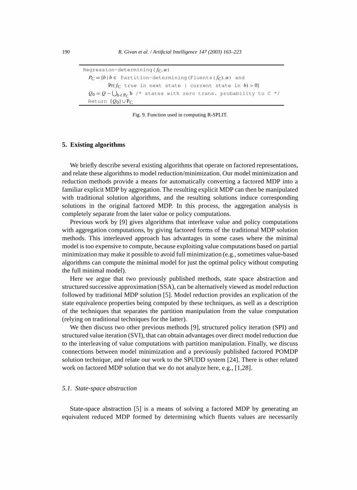
190 R. Givan et al. / Artificial Intelligence 147 (2003) 163–223
Regression-determining(fC, α)
PC = {b | b ∈ Partition-determining(Fluents(fC),α) and
Pr(fC true in next state | current state in b) > 0}Q0 =Q−⋃
b∈PCb /* states with zero trans. probability to C */
Return {Q0} ∪ PC
Fig. 9. Function used in computing R-SPLIT.
5. Existing algorithms
We briefly describe several existing algorithms that operate on factored representations,and relate these algorithms to model reduction/minimization. Our model minimization andreduction methods provide a means for automatically converting a factored MDP into afamiliar explicit MDP by aggregation. The resulting explicit MDP can then be manipulatedwith traditional solution algorithms, and the resulting solutions induce correspondingsolutions in the original factored MDP. In this process, the aggregation analysis iscompletely separate from the later value or policy computations.
Previous work by [9] gives algorithms that interleave value and policy computationswith aggregation computations, by giving factored forms of the traditional MDP solutionmethods. This interleaved approach has advantages in some cases where the minimalmodel is too expensive to compute, because exploiting value computations based on partialminimization may make it possible to avoid full minimization (e.g., sometimes value-basedalgorithms can compute the minimal model for just the optimal policy without computingthe full minimal model).
Here we argue that two previously published methods, state space abstraction andstructured successive approximation (SSA), can be alternatively viewed as model reductionfollowed by traditional MDP solution [5]. Model reduction provides an explication of thestate equivalence properties being computed by these techniques, as well as a descriptionof the techniques that separates the partition manipulation from the value computation(relying on traditional techniques for the latter).
We then discuss two other previous methods [9], structured policy iteration (SPI) andstructured value iteration (SVI), that can obtain advantages over direct model reduction dueto the interleaving of value computations with partition manipulation. Finally, we discussconnections between model minimization and a previously published factored POMDPsolution technique, and relate our work to the SPUDD system [24]. There is other relatedwork on factored MDP solution that we do not analyze here, e.g., [1,28].
5.1. State-space abstraction
State-space abstraction [5] is a means of solving a factored MDP by generating anequivalent reduced MDP formed by determining which fluents values are necessarily
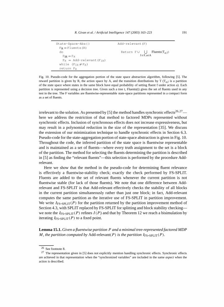
R. Givan et al. / Artificial Intelligence 147 (2003) 163–223 191
State-Space-Abs() Add-relevant(F)
FR = Fluents(R)doFIR = FRFR = Add-relevant(FIR)while (FIR �= FR)return FR
Return F∪ ⋃f∈F,a∈A
Fluents(Ta,f)
Fig. 10. Pseudo-code for the aggregation portion of the state space abstraction algorithm, following [5]. Thereward partition is given by R, the action space by A, and the transition distributions by T (Ta,f is a partitionof the state space where states in the same block have equal probability of setting fluent f under action a). Eachpartition is represented using a decision tree. Given such a tree t, Fluents(t) gives the set of fluents used in anytest in the tree. The F variables are fluentwise-representable state-space partitions represented in a compact formas a set of fluents.
irrelevant to the solution. As presented by [5] the method handles synchronic effects26,27—here we address the restriction of that method to factored MDPs represented withoutsynchronic effects. Inclusion of synchronous effects does not increase expressiveness, butmay result in a polynomial reduction in the size of the representation [35]. We discussthe extension of our minimization technique to handle synchronic effects in Section 6.3.Pseudo-code for the state-aggregation portion of state-space abstraction is given in Fig. 10.Throughout the code, the inferred partition of the state space is fluentwise representableand is maintained as a set of fluents—where every truth assignment to the set is a blockof the partition. The method for selecting the fluents determining the partition is describedin [5] as finding the “relevant fluents”—this selection is performed by the procedure Add-relevant.
Here we show that the method in the pseudo-code for determining fluent relevanceis effectively a fluentwise-stability check; exactly the check performed by FS-SPLIT.Fluents are added to the set of relevant fluents whenever the current partition is notfluentwise stable (for lack of those fluents). We note that one difference between Add-relevant and FS-SPLIT is that Add-relevant effectively checks the stability of all blocksin the current partition simultaneously rather than just one block; in fact, Add-relevantcomputes the same partition as the iterative use of FS-SPLIT in partition improvement.We write IFS-SPLIT(P ) for the partition returned by the partition improvement method ofSection 4.3, with SPLIT replaced by FS-SPLIT for splitting and block stability checking—we note the IFS-SPLIT(P ) refines I (P ) and that by Theorem 12 we reach a bisimulation byiterating IFS-SPLIT(P ) to a fixed point.
Lemma 15.1. Given a fluentwise partition P and a minimal tree-represented factored MDPM , the partition computed by Add-relevant(P ) is the partition IFS-SPLIT(P ).
26 See footnote 8.27 The representation given in [5] does not explicitly mention handling synchronic effects. Synchronic effects
are achieved in that representation when the “synchronized variables” are included in the same aspect when theaction is described.
192 R. Givan et al. / Artificial Intelligence 147 (2003) 163–223
As a result, we conclude that iterating Add-relevant, as in state-space abstraction, is
equivalent to iterating FS-SPLIT as in model reduction.Theorem 15. Given a minimal tree-represented MDP, model reduction using FS-SPLITyields the same partition that state-space abstraction yields, and does so in polynomial-time in the MDP representation size.
Boutilier and Dearden [5] also describe a method of approximation by limiting thefluents that are considered relevant to the reward partition—this idea can also be capturedin the model reduction framework using ideas like those in Section 6.2.
5.2. Structured stochastic dynamic programming—overview
Policy iteration is a well-known technique for finding an optimal policy for an explicitlyrepresented MDP by evaluating the value at each state of a fixed policy and using thosevalues to compute a locally better policy. Iterating this process leads to an optimal policy[42]. In explicit MDPs, the evaluation of each fixed policy can be done with anotherwell-known algorithm called successive approximation, which computes the n-step-to-govalue function for the policy for each n-converging quickly to the infinite-horizon valuefunction for the policy. A related technique, value iteration, computes the n-step-to-govalue function for the optimal policy directly, for each n. Both successive approximationand value iteration converge in the infinite limit to the true value function, and a stoppingcriterion can be designed to indicate when the estimated values are within some giventolerance [42].
Boutilier et al. in [9] describe variants of policy iteration, successive approximation, andvalue iteration designed to work on factored MDP representations, called structured policyiteration (SPI), structured successive approximation (SSA), and structured value iteration(SVI), respectively. As we discuss in detail below, SSA can be understood as a variant ofmodel reduction using the regression splitting operation R-SPLIT described in Section 4.6.Single iterations of SPI can also be understood in this manner: the policy improvementphase can be described using a variant of model reduction, so that SPI can be viewed asiterating policy improvement and SSA, each a model reduction.
These methods can be viewed as performing partition manipulation simultaneously withvalue and/or optimal policy computation—here we will indicate the connection betweenmodel reduction and the partition manipulations performed by these algorithms. If modelreduction is used, the value and/or policy computations are performed on the aggregatemodel after reduction, using standard explicit-model techniques. We note that removingthe value computations from these algorithms yields substantially simpler code; however,computing value functions and policies during reduction allows their use “anytime” even ifreduction is too expensive to complete. The interleaved value computations also allow theaggregation of states that are not equivalent dynamically under all actions. The guaranteeis only that the value will be the same for the optimal28 actions (which will still remain
28 Here, “optimal” refers to being the optimal initial action in a finite horizon policy, where the horizon isextended on each iteration of the method.
R. Givan et al. / Artificial Intelligence 147 (2003) 163–223 193
optimal) but the aggregated model may not be equivalent to the original model for other
actions. Determining which actions are optimal to enable this extra aggregation requiresmaintaining information about state values.SVI is closely similar to model reduction when the tree simplification phase, discussedbelow, is omitted; tree simplification is generally made possible by the interleaved valuecomputations, and can result in significant savings. Each iteration of SPI is understoodusing model reduction restricted to the current policy; however, the full iterative procedureis quite different from model reduction followed by explicit policy iteration. Informally,this is because SPI performs aggregation relative to the different specific policiesencountered, whereas model minimization or reduction aggregates relative to all policies(states must be separated if they differ under any policy).
With both policy and value iteration, model reduction has an advantage in cases wherethe MDP parameters (but not the tree structure, i.e., the partitions) may change frequently,as in some machine learning settings where the parameters are being learned, for example.In such cases, the reduced model does not change when the parameters change,29 so no re-aggregation needs to be done upon parameter change. This observation suggests omittingtree simplification from SVI in such cases.
Another example where model reduction has an advantage over SPI/SVI arises with“exogenous events”. [9] mentions the difficulty in capturing “exogenous events” suchas external user requests in the SPI/SVI approach—such requests have the effect ofchanging the parameters of the reward function, but not the structure, and typicallyrequire re-computing the entire solution when using SPI/SVI. In contrast, the modelreduction approach does not require any new partition manipulation upon changing thereward parameters, since the reduced model is unchanged; only the explicit reduced-modelsolution needs to be re-computed, by traditional methods. One contribution of our work isin explicating the SPI/SVI methods by separating analysis of the value computations fromanalysis of the partition manipulations, as well as connecting the latter to the literature onconcurrent processes and automata theory.
Although the value computations included in SPI and SVI differentiate these methodsfrom model reduction, our methods can still be used to explicate the partition manipulationsperformed by these algorithms. In particular, using the model-reduction form of SSA weconstruct a model-reduction presentation of SPI below. Following [9], throughout thissection we assume that all factored MDPs are represented using decision trees for thepartitions involved in defining the reward and action-transition functions. Moreover, weassume that these trees are minimal in the following sense: if a fluent appears in a tree, thenthe tree could not be modified by simply deleting that fluent (and replacing it with eithersub-tree) without changing the function represented by the tree. Minimality in this sense iseasy to enforce, and without minimality, the algorithms in [9] may do more splitting thanour methods.
29 Assuming an appropriate split operation is used (R-SPLIT or S-SPLIT, for example). If R-SPLIT is beingused, the given “structure” must indicate which parameters are zero and which are non-zero. We note that exactmodel minimization (as opposed to reduction) produces a result that can depend heavily on the model parameters,not just on the structure of parameter dependency.
194 R. Givan et al. / Artificial Intelligence 147 (2003) 163–223
5.3. Structured stochastic dynamic programming—details
Partial pseudo-code for the SSA, SPI, and SVI algorithms is shown in Fig. 11. Here weshow only the partition-manipulation aspects of the algorithms, and only briefly indicatethe somewhat complex associated value computations. We provide pseudo-code for thesealgorithms for reference and for grounding our theorems below, but a full appreciation ofthis section requires familiarity with [9].
We begin our analysis of the connection between SSA/SVI/SPI and model reductionby showing that the partition computed by the function PRegress is closely related to thepartition computed by the function Regression-determining presented earlier, in Fig. 9.Regression-determining computes factored block splitting.
Lemma 16.1. Let V be a tree-represented value function, where PV is the partition givenby the tree. Let α be an action, and for any block C of PV , let ΦC denote the conjunctionof literals describing C. We then have the following:
The partition computed by PRegress(V ,α) is the intersection over all blocks C of PV
of Regression-determining(ΦC,α).
The key subroutines Regress-policy and Regress-action compute factored state-spacepartitions identical to those computed by the I operator (see Section 4.2) under thefollowing assumptions: first, the only actions available are those under consideration(either the single action specified for Regress-action, or the actions specified by thepolicy for Regress-policy); and second, to improve effectiveness and stay within thedecision-tree representation, all block-splitting is done with the structural split operationR-SPLIT. Regress-policy also forcibly splits apart states that select different actions,even if those actions behave identically (see the line QV,π .Tree = π .Tree in Regress-policy).
To formalize these ideas, we need a method of enforcing the first assumption concerningthe available actions. For a fixed policy π and MDP M , we define the π -restricted MDPMπ to be the MDP M modified to have only one action that at each state q has the sametransition behavior as π(q) in M . To model the restriction to a single action α in Regress-action, we consider the policy πα that maps every state to action α, and then use Mπα torestrict to that single action everywhere.
We now define IR-SPLIT(P ) to be the partition returned by partition improvement usingR-SPLIT for splitting, so we can state the following results describing Regress-action andRegress-policy.
Lemma 16.2. Given action α and value function V , Regress-action(V ,α) on MDP M
intersected with V .tree gives the partition computed by IR-SPLIT(V .Tree) on MDP Mπα .
Lemma 16.3. Given policy π and value function V , Regress-policy(V ,π) on MDP M
intersected with V.tree gives the partition computed by IR-SPLIT(V .Tree) on MDP Mπ
intersected with π.Tree.
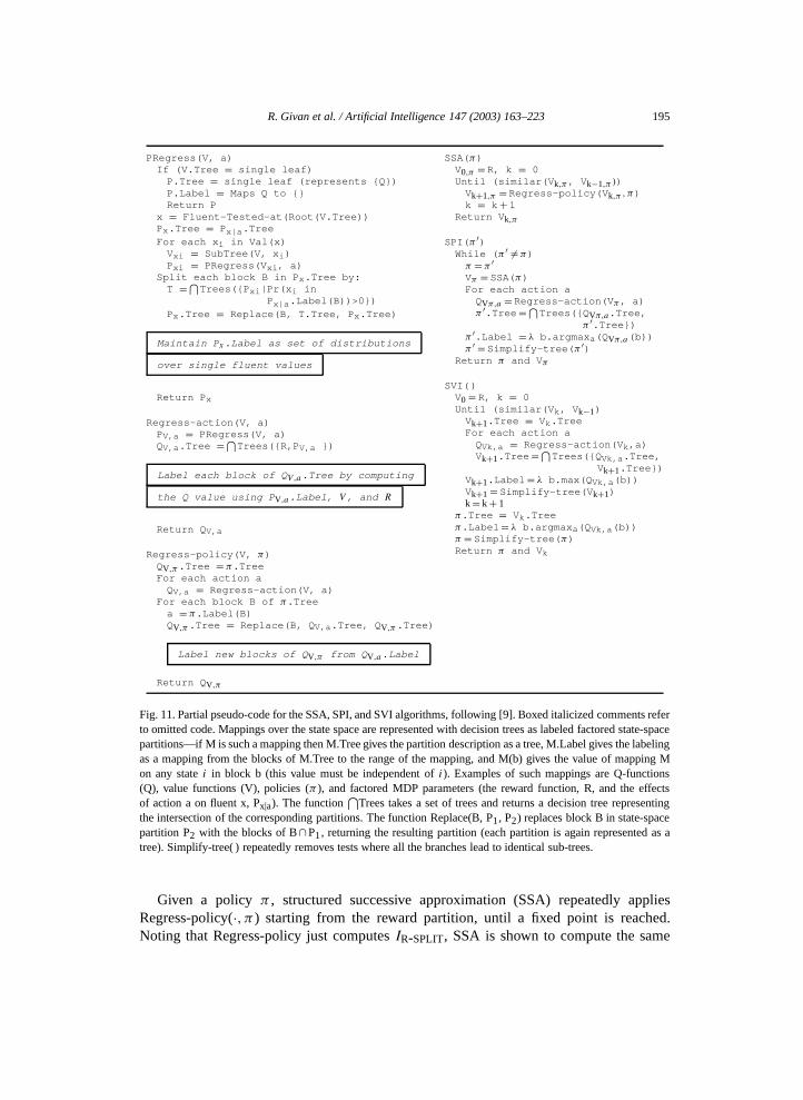
R. Givan et al. / Artificial Intelligence 147 (2003) 163–223 195
PRegress(V, a) SSA(π)
If (V.Tree = single leaf)P.Tree = single leaf (represents {Q})P.Label = Maps Q to {}Return Px = Fluent-Tested-at(Root(V.Tree))Px.Tree = Px|a.TreeFor each xi in Val(x)Vxi = SubTree(V, xi)Pxi = PRegress(Vxi, a)
Split each block B in Px.Tree by:T =⋂
Trees({Pxi|Pr(xi inPx|a.Label(B))>0})
Px.Tree = Replace(B, T.Tree, Px.Tree)
Maintain Px.Label as set of distributions
over single fluent values
Return Px
Regress-action(V, a)PV,a = PRegress(V, a)QV,a.Tree =⋂
Trees({R,PV,a })
Label each block of QV,a.Tree by computing
the Q value using PV,a.Label, V , and R
Return QV,a
Regress-policy(V, π)QV,π.Tree = π.TreeFor each action aQV,a = Regress-action(V, a)
For each block B of π.Treea = π.Label(B)QV,π.Tree = Replace(B, QV,a.Tree, QV,π.Tree)
Label new blocks of QV,π from QV,a.Label
Return QV,π
V0,π = R, k = 0Until (similar(Vk,π, Vk−1,π ))Vk+1,π = Regress-policy(Vk,π , π)k = k+ 1
Return Vk,π
SPI(π ′)While (π ′ �= π)
π = π ′Vπ = SSA(π)For each action aQVπ,a = Regress-action(Vπ, a)π ′.Tree=⋂
Trees({QVπ,a.Tree,π ′.Tree})
π ′.Label = λ b.argmaxa(QVπ,a(b))π ′ = Simplify-tree(π ′)
Return π and Vπ
SVI()V0 = R, k = 0Until (similar(Vk, Vk−1)Vk+1.Tree = Vk.TreeFor each action aQVk,a = Regress-action(Vk,a)Vk+1.Tree=
⋂Trees({QVk,a.Tree,
Vk+1.Tree})Vk+1.Label= λ b.max(QVk,a(b))Vk+1 = Simplify-tree(Vk+1)k= k+ 1
π.Tree = Vk.Treeπ.Label= λ b.argmaxa(QVk,a(b))π = Simplify-tree(π)Return π and Vk
Fig. 11. Partial pseudo-code for the SSA, SPI, and SVI algorithms, following [9]. Boxed italicized comments referto omitted code. Mappings over the state space are represented with decision trees as labeled factored state-spacepartitions—if M is such a mapping then M.Tree gives the partition description as a tree, M.Label gives the labelingas a mapping from the blocks of M.Tree to the range of the mapping, and M(b) gives the value of mapping Mon any state i in block b (this value must be independent of i). Examples of such mappings are Q-functions(Q), value functions (V), policies (π ), and factored MDP parameters (the reward function, R, and the effectsof action a on fluent x, Px|a). The function
⋂Trees takes a set of trees and returns a decision tree representing
the intersection of the corresponding partitions. The function Replace(B, P1, P2) replaces block B in state-spacepartition P2 with the blocks of B∩P1, returning the resulting partition (each partition is again represented as atree). Simplify-tree( ) repeatedly removes tests where all the branches lead to identical sub-trees.
Given a policy π , structured successive approximation (SSA) repeatedly appliesRegress-policy(·,π ) starting from the reward partition, until a fixed point is reached.Noting that Regress-policy just computes IR-SPLIT, SSA is shown to compute the same
196 R. Givan et al. / Artificial Intelligence 147 (2003) 163–223
partition of the state space as partition iteration on the π -restricted MDP using R-SPLIT,
starting from the π -induced partition of the state space.Theorem 16. For any tree-represented MDP M and policy π , SSA(π) produces the sameresulting partition as partition iteration on Mπ using R-SPLIT starting from the partitionπ .Tree.
We note that it follows from Theorem 11 that the resulting partition is a bisimulation, sothat traditional value computation methods can be used on the resulting aggregate modelto compute a factored value function for M .
Policy iteration requires the computation of values to select the policy at each iteration—as a result, model reduction (which does not compute state values, but only aggregations)cannot be viewed alone as performing policy iteration. Here we analyze structured policyiteration as a combination of model reduction, traditional explicit-model techniques, andtree simplification.
Each iteration of structured policy iteration improves the policy π in two steps,analogous to explicit policy iteration: first, the policy π is evaluated using SSA, and thenan improved policy is found relative to π using “structured policy improvement” (which isimplemented by calls to
⋂Trees and Simplify-tree in the pseudo-code). The first of these
steps is equivalent to model reduction on Mπ followed by traditional value iteration, as justdiscussed, yielding a factored value function for π .
Given this value function Vπ , policy improvement is conducted as follows. Thecentral “for” loop in the SPI pseudo-code intersects the partitions returned by Regress-action(Vπ,α) for the different actions α. Noting we have shown that Regress-actioncomputes the IR-SPLIT operation on the partition for Vπ in Mπα , we show here that this“for” loop computes the IR-SPLIT operation for M itself. Once this operation is used tocompute the partition, policy improvement concludes by doing a greedy look-ahead tocompute the block labels (actions) and then simplifying the resulting tree.
Theorem 17. The policy improvement “for” loop in SPI computes IR-SPLIT(Vπ .Tree).
Therefore, each SPI iteration is equivalent to using model reduction and explicit valueiteration to evaluate the policy π , and then partition improvement (IR-SPLIT) followed by agreedy look-ahead and tree-simplification to compute a new policy π . We note that this isnot the most natural way to use model reduction to perform policy iteration—that wouldbe to reduce the entire model to a reduced model using R-SPLIT, and then conduct explicitpolicy iteration on the resulting reduced model. The trade-off between SPI and this moredirect approach is discussed at the beginning of Section 5: SPI benefits in many cases bydoing value computations that allow tree simplification, but model reduction is useful insettings where the aggregation cannot depend on the model parameters but only the modelstructure (i.e., the parameters may change).
To conclude our discussion of structured stochastic dynamic programming, we turn tostructured value iteration, or SVI. Perhaps, the most natural way to use model reductionto perform value iteration would be to compute a reduced model (say using S-SPLIT) andthen perform explicit value iteration on that model. It turns out that SVI computes exactly
R. Givan et al. / Artificial Intelligence 147 (2003) 163–223 197
this reduced model (while simultaneously performing value computations) if we omit the
tree simplification step (Simplify-tree). This can be seen by noting that the “for” loop inSVI computes IR-SPLIT, just as the “for” loop in SPI does—in this case, SVI iterates thiscomputation starting from the reward function (using the “until” loop) until the reducedmodel is computed,30 after which SVI is just performing standard value iteration on thatmodel. We conclude that, without tree simplification, SVI is essentially equivalent to modelreduction using R-SPLIT followed by value iteration. Adding tree simplification to SVI hasadvantages and disadvantages similar to the tree simplification in SPI, as discussed above.If desired, SVI with tree simplification can be modeled using partition improvement withappropriate value function labeling alternated with tree simplification.5.4. Partially observable MDPs
The simplest way of using model-reduction techniques to solve partially observableMDPs (POMDPs) is to apply the model-minimization algorithm to the underlying fullyobservable MDP using an initial partition that distinguishes on the basis of both rewardand observation model. The reduced model can then be solved using a standard POMDPalgorithm [11,33,39,43]. We conjecture that the factored POMDP algorithm described in[4] can be analyzed using model reduction in a manner similar to the analysis of SVIpresented above.
5.5. SPUDD
More recent work improving structured dynamic programming, e.g., SPUDD [24], hasprimarily been concerned with changing the underlying representation from decision treesto decision diagrams. Since our algorithm is developed independently of the representation,model reduction is well defined for partitions represented as decision diagrams—noextension is needed. Rather than repeating all the analytic results shown above forstructured dynamic programming again, for decision diagrams, we instead note that similaranalytical results can be developed, comparing model minimization to SPUDD. We expectthat empirical comparisons similar to those shown below can be obtained as well, but wedo not yet have a decision diagram implementation.
6. Extensions and related work
6.1. Action equivalence for large action spaces
We have extended the notion of stochastic bisimilarity to include equivalence betweenactions that behave identically [15]. Intuitively, two actions that have identical definitionscan be collapsed into one. More than this though, once a state space equivalence relationhas been selected, two actions that have different definitions may behave the same, once
30 We assume the “Similar(V,V ′)” test in SVI returns “false” if the corresponding partitions are different.
198 R. Givan et al. / Artificial Intelligence 147 (2003) 163–223
groups of equivalent states are aggregated. We wish to define the partition of the action
space that results from a stochastic bisimulation using this intuition. Given an MDPM = 〈Q,A,T ,R〉 and a relation E ⊆ Q × Q, we say that two actions α1 and α2 aredynamically bisimilar with respect to E if for every two states i, j ∈ Q we have thatT (i,α1, j/E) = T (i,α2, j/E). Given this equivalence relation on actions, we can thendefine a dynamic quotient MDP that aggregates both the state and action space. Givenan MDP M = 〈Q,A,T ,R〉 and a bisimulation E ⊆Q ×Q, the dynamic quotient MDPM/(E,D), where D is the dynamic bisimilarity relation with respect to E, is definedto be the machine 〈Q/E,A/D,T ′,R′〉 such that T ′(i/E,α/D, j/E)= T (i,α, j/E) andR′(i/E) = R(i) where the choice of i and j does not affect T or R because E is abisimulation, and the choice of α does not affect T by the definition of D.One approach to computing a dynamic quotient MDP is to first compute a stochasticbisimulation and then compute the dynamic bisimilarity relation with respect to thatbisimulation. However, this approach fails to exploit the possible reductions in the actionspace (by equivalence) during the construction of the stochastic bisimulation. Specifically,the iterative construction of the stochastic bisimilarity relation described in this paperrequires, at each iteration, a computation for each action. If the action space can be groupedinto exponentially fewer equivalence classes of actions, this “per action” computation canbe replaced by a “per equivalence class of actions” computation, with possible exponentialtime savings. All of this assumes we can cheaply compute the dynamic bisimilarity relationD, which will depend entirely on the representation used for the MDP and the relationE. We do not consider this issue here, but in [15] we present representations for MDPsthat allow the effective computation of dynamic bisimilarity for many MDPs, and givean algorithm that exploits dynamic bisimilarity to achieve possibly exponential savings inruntime (over that from model reduction alone).
6.2. Approximate model minimization
One of the foci of this paper has been to translate some of the efficiency of representingan MDP in a compact form into efficiency in computing an optimal policy for that MDP.The resulting computational savings can be explained in terms of finding a bisimulationover the state space, and using the corresponding partition to induce a smaller MDPthat is equivalent to the original MDP in a well-defined sense. The reduced MDP statescorrespond to groups of states from the original MDP that behave the same under allpolicies, and thus the original and reduced MDP yield the same optimal policies and statevalues. Despite reducing the MDP with this approach, the resulting minimal model in manycases may still be exponentially larger than the original compact MDP representation—implying that in some cases the computational cost of solving the reduced MDP is stillrather daunting.
One approach to overcoming this computational cost is to relax the definition ofequivalence on states. This relaxation can be done by allowing the aggregation of statesinto the same “equivalence” class even though their transition probabilities to other blocksare different, so long as they are approximately the same (i.e., within ε of each other, forsome parameter ε). We call the resulting partition an ε-stable partition—such a partitiongenerally induces an aggregate MDP that is much smaller than the exact minimal model.
R. Givan et al. / Artificial Intelligence 147 (2003) 163–223 199
Use of this approach does have its drawbacks: the reduced model is not equivalent to the
original MDP, but only approximately equivalent. Solutions resulting from approximatemodel minimization thus may not be optimal but will typically be approximately optimal.For further information on how to carry out approximate model minimization/reductionsee [14].6.3. Handling synchronic effects
We first extend our representation of a factored MDP M = 〈F,A,TF ,RF 〉 given inSection 2.3 to represent synchronic effects (correlations between the effects of an actionon different fluents). We change only the definition of TF from our factored representationwithout synchronic effects. As before, the state space Q is given by the set of statefluents F . Following Bayesian belief network practice, the fluents F are now orderedas f1, . . . , fn—the distribution describing the effects of an action on a fluent fi willbe allowed to depend on the post-action values of fluents fj for j less than i , and thecompactness of the resulting representation will in general depend heavily on the orderingchosen.
We assume that a “parent” relationship is defined for the fluents, as in a Bayesiannetwork, such that for each fluent fi , Parents(fi,α) is a set of fluents earlier in the orderingf1, . . . , fn such that the value of fi after taking action α is independent of the post-actionvalue of any other fluent fj , given post-action values for Parents(fi,α). We then define theAncestors(fi,α) to give the set of fluents that are transitively parents of fi for action α,along with fi itself. The state-transition distribution of a factored MDP is now specifiedby giving a factored partition TF (α,fi) of Q for each fluent fi and action α, where eachpartition block is labeled with a factored joint probability distribution over Ancestors(fi,α)giving the probability that each assignment to Ancestors(fi,α) will result when taking α
from the labeled block. The distributions TF (α,fi ) must obey a consistency constraint: foreach action α and fluents f and f ′ such that f ′ ∈ Parents(f,α), the distribution TF (α,f
′)must be the same as the distribution TF (α,f ) marginalized to the fluents Ancestors(f ′).One way to achieve this consistency is to represent each factored conditional probabilitydistribution as a product (as in a Bayesian network), such that the distribution for a fluentincludes every factor used in the product of any of that fluent’s parents31 (i.e., the Bayesiannetwork for fluent f contains the Bayesian networks for the parents of f ).
Given this representation for a synchronous-effect factored MDP, model reduction usingS-SPLIT, F-SPLIT, or FS-SPLIT can be carried out just as specified above. This is becausethese split methods do not depend on the partition labels in the action descriptions, but onlyon the partitions themselves. Exact splitting with SPLIT requires using the joint probabilitydistribution labels to combine blocks that are “coincidentally” alike after S-SPLIT. This
31 Conversion to this factored MDP representation from the more familiar (and very similar) dynamic Bayesiannetworks with synchronous effects is straightforward [35], but may involve an exponential growth in size incomputing the required state-space partitions. It is possible to design a similar labeled-partition representation thatavoids this growth, but applying model minimization appears to require the exponentially larger representation.The synchronous-effect methods presented in [9] also encounter exponential size growth when “summing outpost-action influences”.
200 R. Givan et al. / Artificial Intelligence 147 (2003) 163–223
combination is similar in spirit to that described for the independent action effects case near
the end of Section 4.4, and we leave this generalization as an exercise for the reader. Modelreduction using R-SPLIT requires adding only an inference algorithm for determiningwhether a joint probability distribution assigns a probability of zero to a given formula—for the key case of distributions in chain-rule product form (i.e., like Bayesian networks)and formulas that are conjunctions of literals, such algorithms are generally well known(e.g., [41]).6.4. Other related work
The basic idea of computing reduced equivalent models has its origins in automatatheory [22] and stochastic processes [27]. Our work can also be viewed as a stochasticgeneralization of recent work in computer-aided verification via model checking [10,31].In addition, the goals of our work are similar to goals of [17], which presents an onlinelearning method using a factored representation to learn about blocks of states, using aregression operator similar to our block splitting operation.
The approximation of an optimal policy discussed in the last section is just one of manyapproximation approaches. Boutilier and Dearden in [6] gives approximate versions of SPIand SVI by sometimes allowing states with similar, but different, values to be aggregatedinto the same leaf of a value-function tree. This additional aggregation is achieved bypruning value trees, replacing sub-trees whose values differ by at most ε by leaves whoselabel may be either an average value for the sub-tree or a range of values subsumingall the values of the sub-tree. Koller and Parr in [28] propose a very different factoredvalue function representation—value functions are represented as a linear combinationof the factored value functions used here, and a policy iteration method is given for thisdecomposed value function method. Note that this representation can assign exponentiallymany different values over the state space with a polynomial-size decomposition, unlikeour labeled factored partitions or the more familiar decision-tree representations for valuefunctions. Large state spaces have also been dealt with approximately by trajectorysampling in [26], and elsewhere.
7. Empirical investigation
We have explored the theory of model minimization; here we provide some dataon its performance on simple synthetic domains. We have constructed a non-optimizedimplementation using DNF formulas to represent blocks—using S-SPLIT to construct areduced, equivalent model. We used this implementation to conduct experiments on theLinear, Expon, and Coffee domains used in the previous evaluation of structured dynamicprogramming [9], and compare the reduced-model sizes found by our technique to the sizeof the value-function representation produced by structured dynamic programming (SVI,in particular). We use the number of leaves in the decision-tree value function produced bySVI as a measure of the size of the representation.
R. Givan et al. / Artificial Intelligence 147 (2003) 163–223 201
We now briefly describe these domains.32 The Linear domains, Linear3 through
Linear9, have between three and nine ordered state fluents, respectively. For each statefluent, the domain provides an action that sets that fluent to “true” while setting all fluentslater in the order to “false”. Reward is obtained only when all state fluents are “true”.The Linear domains were designed to show the strengths of the structured-dynamic-programming algorithms—due to our similarity to these approaches, we expected to seegood results on these domains. The Expon domains, Expon3 through Expon9, are similarto the Linear domains, except that the action corresponding to each state fluent sets thatfluent to “true”, if all later fluents are “true”, and sets it “false” otherwise. (In eithercase, as before, it sets all later fluents to “false”.) To reach reward, these actions mustbe used to “count” through the binary representations of the states, so we expect everystate to behave uniquely. The Expon domains were designed to exploit the weaknesses ofstructured dynamic programming, so, we expected little reduction in state space size.The Coffee domain has six state fluents (has-user-coffee, has-robot-coffee, wet, raining,have-umbrella, and location) and four actions (move, give-coffee, buy-coffee, and get-umbrella). The move action has a 0.9 chance of moving the robot between the office andstore locations, with an 0.9 chance of getting the robot wet if it is raining, unless the robothas the umbrella, which reduces that chance to 0.1. If the robot is in the office with coffee,the give-coffee action has a 0.8 chance of giving the user coffee and an (independent) 0.9chance of the robot losing the coffee. If the robot is at the store, give-coffee has a 0.8 chanceof the robot losing the coffee, with no chance of providing any to the user. Buy-coffee hasa 0.9 chance of getting the robot coffee, if the robot is in the store. Get-umbrella has a 0.9chance of getting the robot the umbrella, when in the office. There is a large reward if theuser has coffee and a small one if the robot is not wet.
These domains are, of course, much smaller than what will typically be seen in realapplications, but they illustrate the range of possible results from our technique, andallow for a comparison to other current approaches, in particular to structured dynamicprogramming. The results obtained in our experiments are shown in Fig. 12, and are asexpected—the Linear domains show a linear increase in the size of the reduced model withrespect the number of variables (i.e., an exponential amount of compression), whereas theExpon domains show no reduction in model size, and remain exponential in the numberof variables. Structured dynamic programming, specifically SVI, performs identically (onboth Linear and Expon domains), showing that we are indeed factoring that method into amodel-reduction phase, followed by any traditional solution technique.
The Coffee domain shows a substantial savings, with the reduced MDP being about athird the size of the original, and very similar in size to the SVI-produced value function,but not identical. The difference in the Coffee domain results from model-reduction
32 Complete details of the Coffee domain and some Linear and Expon domains can be found onlineat http://www.cs.ubc.ca/spider/jhoey/spudd/spudd.html. Note that this website also contains some “factory”domains. We do not include these domains in our tests because both our model reduction implementation(using S-SPLIT) and the web-available SPUDD implementation are unable to solve them exactly in the availablememory. Approximation methods could be added to either approach in order to handle the factory domains,however these approximation techniques will not be discussed further here. (We note that SPUDD has suchapproximation built in, and can analyze the factory domains using it.)
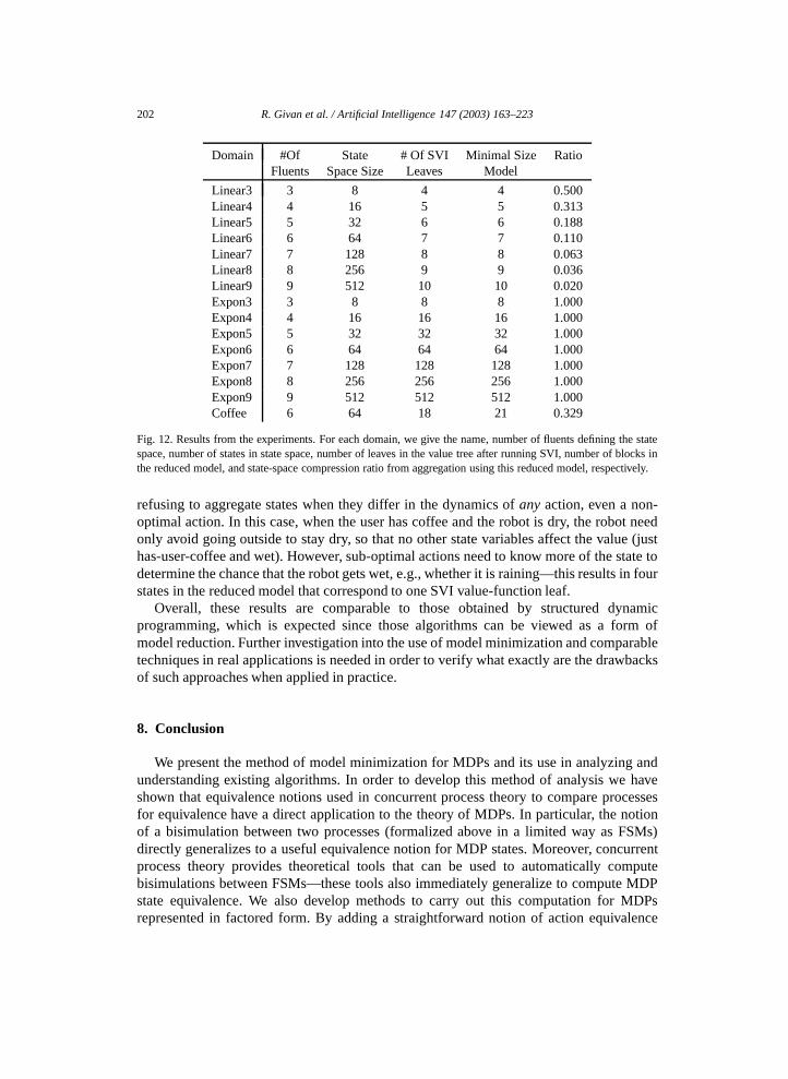
202 R. Givan et al. / Artificial Intelligence 147 (2003) 163–223
Domain #Of State # Of SVI Minimal Size Ratio
Fluents Space Size Leaves ModelLinear3 3 8 4 4 0.500Linear4 4 16 5 5 0.313Linear5 5 32 6 6 0.188Linear6 6 64 7 7 0.110Linear7 7 128 8 8 0.063Linear8 8 256 9 9 0.036Linear9 9 512 10 10 0.020Expon3 3 8 8 8 1.000Expon4 4 16 16 16 1.000Expon5 5 32 32 32 1.000Expon6 6 64 64 64 1.000Expon7 7 128 128 128 1.000Expon8 8 256 256 256 1.000Expon9 9 512 512 512 1.000Coffee 6 64 18 21 0.329
Fig. 12. Results from the experiments. For each domain, we give the name, number of fluents defining the statespace, number of states in state space, number of leaves in the value tree after running SVI, number of blocks inthe reduced model, and state-space compression ratio from aggregation using this reduced model, respectively.
refusing to aggregate states when they differ in the dynamics of any action, even a non-optimal action. In this case, when the user has coffee and the robot is dry, the robot needonly avoid going outside to stay dry, so that no other state variables affect the value (justhas-user-coffee and wet). However, sub-optimal actions need to know more of the state todetermine the chance that the robot gets wet, e.g., whether it is raining—this results in fourstates in the reduced model that correspond to one SVI value-function leaf.
Overall, these results are comparable to those obtained by structured dynamicprogramming, which is expected since those algorithms can be viewed as a form ofmodel reduction. Further investigation into the use of model minimization and comparabletechniques in real applications is needed in order to verify what exactly are the drawbacksof such approaches when applied in practice.
8. Conclusion
We present the method of model minimization for MDPs and its use in analyzing andunderstanding existing algorithms. In order to develop this method of analysis we haveshown that equivalence notions used in concurrent process theory to compare processesfor equivalence have a direct application to the theory of MDPs. In particular, the notionof a bisimulation between two processes (formalized above in a limited way as FSMs)directly generalizes to a useful equivalence notion for MDP states. Moreover, concurrentprocess theory provides theoretical tools that can be used to automatically computebisimulations between FSMs—these tools also immediately generalize to compute MDPstate equivalence. We also develop methods to carry out this computation for MDPsrepresented in factored form. By adding a straightforward notion of action equivalence
R. Givan et al. / Artificial Intelligence 147 (2003) 163–223 203
relative to a bisimulation, we can also use the notion of bisimulation to aggregate a large
action space. These methods also lend themselves naturally to approximation, as we havediscussed elsewhere in [14].Appendix A
Lemma 4.1. The reflexive symmetric transitive closure of a stochastic bisimulationbetween any two MDPs M = 〈Q,A,T ,R〉 and M ′ = 〈Q′,A,T ′,R′〉 restricted to Q×Q
is itself a stochastic bisimulation between M and itself.
Proof. Let E1 be a stochastic bisimulation between the MDPs M = 〈Q,A,T ,R〉 andM ′ = 〈Q′,A,T ′,R′〉 and let E2 be the reflexive symmetric transitive closure of E1restricted to Q×Q. We show that E2 is a stochastic bisimulation.
Consider i and j in Q such that E2(i, j). We note that the definition of E2 as thereflexive symmetric transitive closure of E1 ensures that there is a (possibly empty) path ofarcs in E1, ignoring arc direction, from i to j . Likewise there must be a path of arcs in E1between any two states in i/E2 or any two states in j/E2. A simple induction on the lengthof an arbitrary path of E1 arcs shows that any two states related by such a path have thesame R (or R′) values, because E1(i
′, j ′) implies R(i ′)= R′(j ′). It follows that R(i/E2)
and R(j/E2) are well defined and equal, as desired in showing that E2 is a bisimulation.To show the transition-model properties that imply that E2 is a bisimulation, we first
note that the sets i/E1 and i/E2 (and likewise j/E1 and j/E2) are identical by definition.We must show that for any i ′ ∈ Q and j ′ ∈ Q such that E2(i
′, j ′), the block transitionprobabilities T (i,α, i ′/E2) and T (j,α, j ′/E2) are equal. As just observed, it suffices toshow that T (i,α, i ′/E1) and T (j,α, j ′/E1) are equal. This follows by induction on thesum of the length of the shortest E1 path from i ′ to j ′ and the length of the shortest E1path from i to j (ignoring arc direction)—this induction iterates the fact that for any actionα, any x, x ′ ∈Q and y, y ′ ∈Q′, E1(x, y) and E1(x
′, y ′) together imply that T (x,α, x ′/E1)
and T ′(y,α, y ′/E1) are equal, since E1 is a bisimulation. ✷Lemma 4.2. The union of two stochastic bisimulations between the same pair of MDPs isalso a stochastic bisimulation between those MDPs.
Proof. Let E1 and E2 be two stochastic bisimulations between the same pair of MDPsM = 〈Q,A,T ,R〉 and M ′ = 〈Q′,A,T ′,R′〉 and let E be the union of those stochasticbisimulations (i.e., the union of the sets of pairs of states related by those bisimulations).We now show that E is a stochastic bisimulation. We write E∗ for the reflexive symmetrictransitive closure of E. Consider i ∈Q and j ∈Q′ such that E(i, j).
That R(i/E) and R′(j/E) are well defined and equal to each other is implied by thefollowing assertion. For any i ′ and j ′ in Q ∪ Q′ such that E∗(i ′, j ′),R′′(i ′) = R′′(j ′),where R′′ is defined on Q ∪ Q′ by R on Q and by R′ on Q′. This assertion is shownby induction on the length of the B-path between i ′ and j ′, iterating the fact thateither E1(i
′′, j ′′) or E2(i′′, j ′′) implies R(i ′′) = R′(j ′′) because E1 and E2 are both
bisimulations.
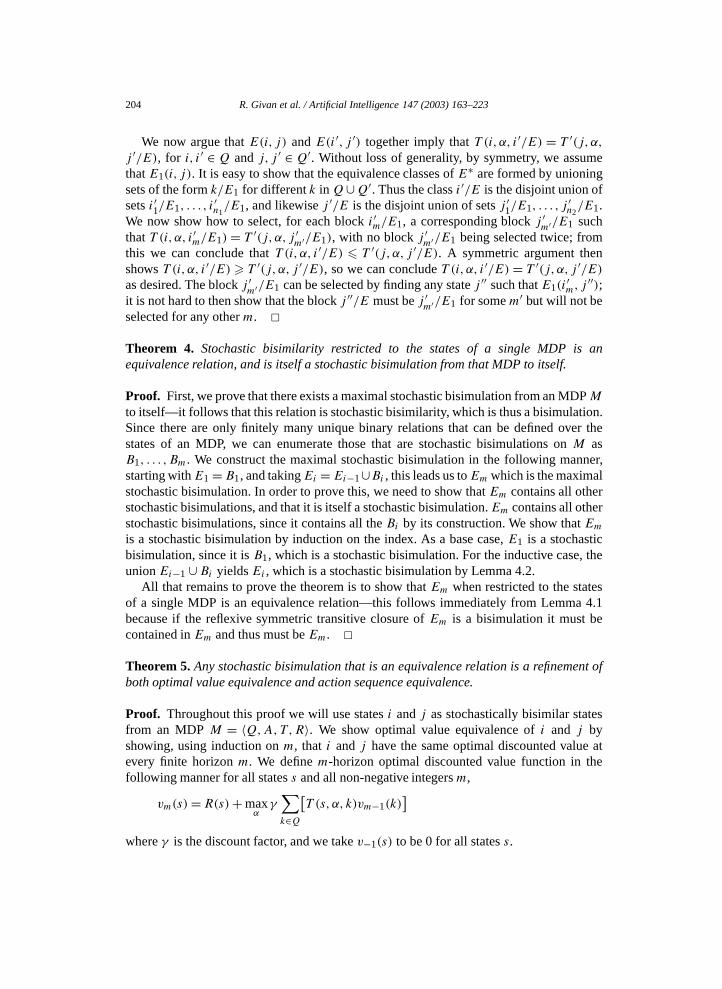
204 R. Givan et al. / Artificial Intelligence 147 (2003) 163–223
We now argue that E(i, j) and E(i ′, j ′) together imply that T (i,α, i ′/E) = T ′(j,α,
j ′/E), for i, i ′ ∈ Q and j, j ′ ∈ Q′. Without loss of generality, by symmetry, we assumethat E1(i, j). It is easy to show that the equivalence classes of E∗ are formed by unioningsets of the form k/E1 for different k in Q∪Q′. Thus the class i ′/E is the disjoint union ofsets i ′1/E1, . . . , i′n1/E1, and likewise j ′/E is the disjoint union of sets j ′1/E1, . . . , j
′n2/E1.
We now show how to select, for each block i ′m/E1, a corresponding block j ′m′/E1 such
that T (i,α, i ′m/E1)= T ′(j,α, j ′m′/E1), with no block j ′
m′/E1 being selected twice; fromthis we can conclude that T (i,α, i ′/E) � T ′(j,α, j ′/E). A symmetric argument thenshows T (i,α, i ′/E) � T ′(j,α, j ′/E), so we can conclude T (i,α, i ′/E) = T ′(j,α, j ′/E)
as desired. The block j ′m′/E1 can be selected by finding any state j ′′ such that E1(i
′m, j
′′);it is not hard to then show that the block j ′′/E must be j ′
m′/E1 for some m′ but will not beselected for any other m. ✷Theorem 4. Stochastic bisimilarity restricted to the states of a single MDP is anequivalence relation, and is itself a stochastic bisimulation from that MDP to itself.
Proof. First, we prove that there exists a maximal stochastic bisimulation from an MDP M
to itself—it follows that this relation is stochastic bisimilarity, which is thus a bisimulation.Since there are only finitely many unique binary relations that can be defined over thestates of an MDP, we can enumerate those that are stochastic bisimulations on M asB1, . . . ,Bm. We construct the maximal stochastic bisimulation in the following manner,starting with E1 = B1, and taking Ei = Ei−1∪Bi , this leads us to Em which is the maximalstochastic bisimulation. In order to prove this, we need to show that Em contains all otherstochastic bisimulations, and that it is itself a stochastic bisimulation. Em contains all otherstochastic bisimulations, since it contains all the Bi by its construction. We show that Em
is a stochastic bisimulation by induction on the index. As a base case, E1 is a stochasticbisimulation, since it is B1, which is a stochastic bisimulation. For the inductive case, theunion Ei−1 ∪Bi yields Ei , which is a stochastic bisimulation by Lemma 4.2.
All that remains to prove the theorem is to show that Em when restricted to the statesof a single MDP is an equivalence relation—this follows immediately from Lemma 4.1because if the reflexive symmetric transitive closure of Em is a bisimulation it must becontained in Em and thus must be Em. ✷Theorem 5. Any stochastic bisimulation that is an equivalence relation is a refinement ofboth optimal value equivalence and action sequence equivalence.
Proof. Throughout this proof we will use states i and j as stochastically bisimilar statesfrom an MDP M = 〈Q,A,T ,R〉. We show optimal value equivalence of i and j byshowing, using induction on m, that i and j have the same optimal discounted value atevery finite horizon m. We define m-horizon optimal discounted value function in thefollowing manner for all states s and all non-negative integers m,
vm(s)=R(s)+maxα
γ∑k∈Q
[T (s,α, k)vm−1(k)
]where γ is the discount factor, and we take v−1(s) to be 0 for all states s.

R. Givan et al. / Artificial Intelligence 147 (2003) 163–223 205
For the base case take m = 0. In this case the value function for any state is just the
reward for that state, v0(s) = R(s). Since states i and j are stochastically bisimilar weknow that R(i)= R(j), and so that v0(i)= v0(j), as desired. For the inductive case, wedefine the m-horizon Q-value33 for any state s, action α, and non-negative integer m, byqm(s,α)=R(s)+ γ∑k∈Q
[T (s,α, k)vm−1(k)
].
Let E be stochastic bisimilarity. Using the induction hypothesis, we have for any action α,
qm(i,α) = R(i)+ γ∑k∈Q
[T (i,α, k)vm−1(k)
]
= R(i)+ γ∑
b∈Q/E
[T (i,α, b)vm−1(b)
]
= R(j)+ γ∑
b′∈Q/E
[T (j,α, b′)vm−1(b
′)]
= R(j)+ γ∑k∈Q
[T (j,α, k)vm−1(k)
]= qm(j,α).
Since for any state s, vm(s)=maxα qm(s,α), it follows that vm(i)= vm(j), as desired.We now show that i and j are action-sequence equivalent by induction on the length m
of the action sequence—we show that for any action sequence α1, . . . , αm, the distributionover sequences of rewards attained by following α1, . . . , αm is the same for i and j . Wetake φs,m(!α) to be a random variable ranging over reward sequences of length m, with thedistribution generated from starting state s following action sequence !α.
For the base case, we take m= 0 and consider the empty sequence ε of actions. Here,the reward sequence φs,0(ε) is deterministically the empty sequence—implying that φi,0(ε)and φj,0(ε) have identical distributions as desired.
For the inductive case, consider action sequence !α = α1, . . . , αm. We note that for anystate s, we have that Pr(φs,m(!α)= r1, . . . , rm) is equal to
Pr(φs,1(α1)= r1
) ∑b∈Q/E
T (s,α1, b)(φb,m−1(α2, . . . , αm)= r2, . . . , rm
),
where φb,n(!α) is defined to be φs,n(!α) for some state s ∈ b, and the choice of s does notaffect the value of φb,n(!α) for n < m by the induction hypothesis. We apply this equationfor s equal to i and for s equal to j , and show that the right-hand sides are equal in the twocases. First, we note that the probability that φs,1(α1) equals r1 in the above equationis either zero or one, depending on whether R(s) is r1, and that R(i) = R(j) since i
and j are stochastically bisimilar. Then, the fact that T (i,α1, b) = T (j,α1, b) for eachblock b (because E is a bisimulation) gives Pr(φi,m(!α) = r1, . . . , rm) = Pr(φj,m(!α) =r1, . . . , rm), concluding the inductive case. Thus, stochastic bisimilarity refines action-sequence equivalence. ✷
33 Our use of the standard terminology “Q-function” does not imply any connection to the state space Q.
206 R. Givan et al. / Artificial Intelligence 147 (2003) 163–223
Theorem 6. The reflexive, symmetric, transitive closure of any stochastic bisimulation from
MDP M = 〈Q,A,T ,R〉 to any MDP, restricted to Q × Q, is an equivalence relationE ⊆Q×Q that is a stochastic bisimulation from M to M .Proof. This follows directly from Lemma 4.1, along with the fact that restricting anequivalence relation to a sub-domain preserves the equivalence relation property. ✷Theorem 7. Given an MDP M = 〈Q,A,T ,R〉 and an equivalence relation E ⊆Q×Q
that is a stochastic bisimulation, each state i in Q is stochastically bisimilar to the statei/E in M/E. Moreover, any optimal policy of M/E induces an optimal policy in theoriginal MDP.
Proof. Let M/E = 〈Q/E,A,T ′,R′〉. First we prove that any i ∈ Q is stochasticallybisimilar to i/E in M/E. Let Z be the relation over Q × Q/E that contains only thepairs (i, i/E) for each i ∈Q. We show Z is a stochastic bisimulation from M to M/E.
Select i ∈ Q and j ∈ Q/E such that Z(i, j). We note that i/Z equals both i/E andj , and that j/Z is the set {j }. It follows that the rewards R(i/Z) and R′(j/Z) are welldefined and equal, since E is a stochastic bisimulation. Now select action α ∈ A, statei ′ ∈Q and state j ′ ∈Q/E such that Z(i ′, j ′). Noting that T (i,α, i ′/Z)= T (i,α, i ′/E)=T ′(i/E,α, i ′/E) = T ′(j,α, j ′) = T ′(j,α, j ′/Z), we conclude Z is a bisimulation andtherefore that i and i/E are stochastically bisimilar.
As above in the proof of Theorem 5, define the Q-value for any state s and action α bygiving q(s,α) as the sum of R(s) and γ
∑k∈Q[T (s,α, k)v∗(k)]. We now show that any
optimal action for state i/E in Q/E is an optimal action for state i in Q. To show this, weshow that the Q-value for arbitrary action α in state i/E is the same as the Q-value for αin state i . We conclude
q(i/E,α) = R′(i/E)+ γ∑
j/E∈Q/E
T ′(i/E,α, j/E)v∗(j/E)
= R(i)+ γ∑
j/E∈Q/E
T (i,α, j/E)v∗(j/E)
= R(i)+ γ∑s∈Q
T (i,α, s)v∗(s)= q(i, α) in M.
The second line follows via the definition of , with for R′ and T ′, and the third line via thedefinition of block transition probability and the equality of values within a block (implicitin the proof of Theorem 5). This Q-value equivalence yields our theorem. ✷Lemma 8.1. Given equivalence relation E on Q and states p and q such that T (p,α,C) �=T (q,α,C) for some action α and block C of E, p and q are not related by any stochasticbisimulation refining E.
Proof. Suppose not. Let B and C denote blocks of the partition of Q induced by E, let α beany action in A, and let p and q denote states in blockB such that T (p,α,C) �= T (q,α,C).Let E′ be a stochastic bisimulation refining E such that p and q are in the same block
R. Givan et al. / Artificial Intelligence 147 (2003) 163–223 207
in E′. Let {C1, . . . ,Ck} be the set of blocks in E′ that refine C. Because E′ is a stochastic
bisimulation, for each block D in E′, T (p,α,D)= T (q,α,D). Summing this fact over allthe blocks Ci we derive the following equation, contradicting T (p,α,C) �= T (q,α,C):T (p,α,C)=∑
1�i�k
T (p,α,Ci)=∑
1�i�k
T (q,α,Ci)= T (q,α,C). ✷
Corollary 8.2. Let E be an equivalence relation on Q,B a block in E, and C a unionof blocks from E. Every bisimulation on Q that refines E is a refinement of the partitionSPLIT(B,C,E).
Proof. Let E be an equivalence relation on Q,B a block in E, and C be the unionof blocks C1 thru Cn from E. Let E′ be a stochastic bisimulation that refines E. Notethat SPLIT(B,C,E) will only split states i and j if either R(i) �= R(j) or T (i,α,C) �=T (j,α,C), by definition. But if R(i) �= R(j) then i/E′ �= j/E′ since E′ is a stochasticbisimulation. And if T (i,α,C) �= T (j,α,C), then there must be some k such thatT (i,α,Ck) �= T (j,α,Ck), because for any state s, T (s,α,C) = ∑
1�m�n T (s,α,Cm).Therefore, we can conclude by Lemma 8.1 that i/E′ �= j/E′. ✷Theorem 8. Partition iteration and model minimization both compute stochastic bisimilar-ity.
Proof. Partition iteration and model minimization both terminate with a partition P forwhich SPLIT(B,C,P )= P for any blocks B and C in P . SPLIT(B,C,P ) will split anyblock B containing a pair of states i and j for which either R(i) �= R(j) or T (i,α,C) �=T (j,α,C). So any partition returned by partition iteration or model minimization mustbe a stochastic bisimulation. Since both model minimization and partition iteration startfrom the trivial {Q} partition, and each only refines the partition by applying the SPLIToperator to blocks in the partition, we can conclude by Corollary 8.2 that each partitionencountered, including the resulting partition, must contain stochastic bisimilarity. Theresulting partition, being a stochastic bisimulation, must be stochastic bisimilarity. ✷Theorem 9. Model reduction returns a stochastic bisimulation.
Proof. Since model reduction always splits at least as much as model minimization, due tothe definition of stability, it must be the case that the partition returned by model reductionis a refinement of the partition returned by the model minimization algorithm, i.e.,stochastic bisimilarity according to Theorem 8. Any such relation has the reward propertiesrequired of stochastic bisimulations. The transition-model properties follow immediatelyfrom the stability of all blocks in the resulting partition, which is a consequence of the exittest of the final “while” loop in the algorithm. ✷Corollary 9.1. The optimal policy for the quotient model produced by model reductioninduces an optimal policy for the original MDP.
Proof. Follows directly from Theorems 7 and 9. ✷
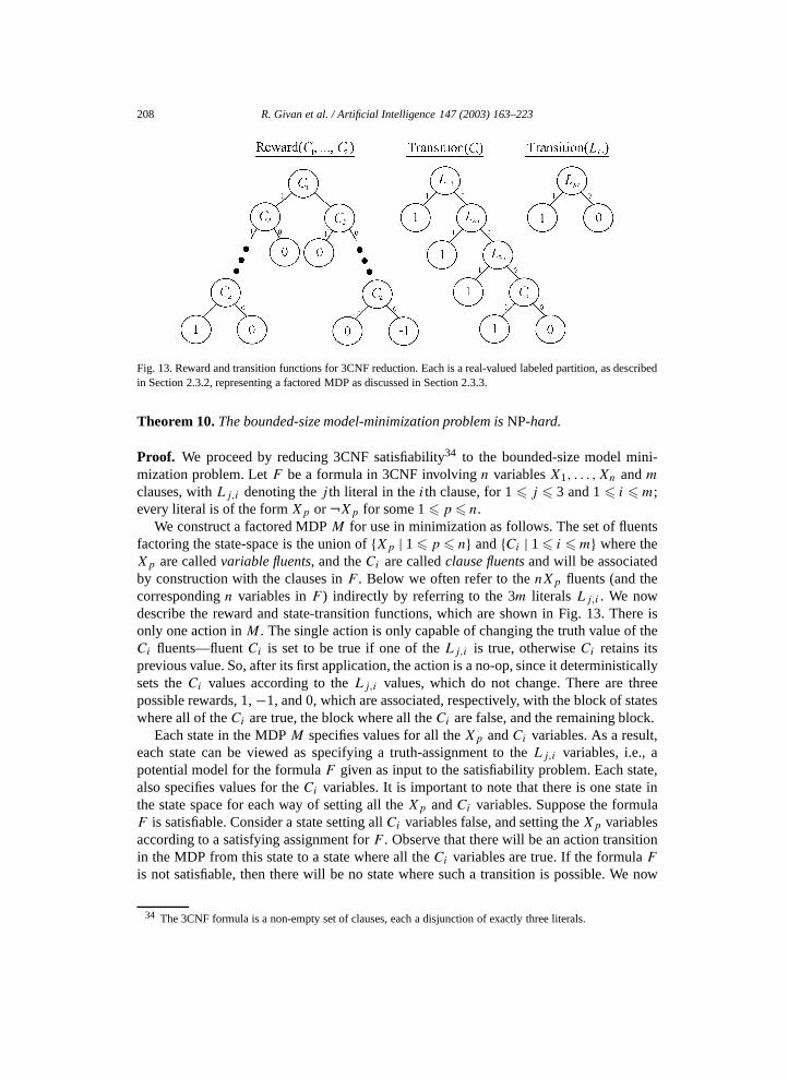
208 R. Givan et al. / Artificial Intelligence 147 (2003) 163–223
Fig. 13. Reward and transition functions for 3CNF reduction. Each is a real-valued labeled partition, as describedin Section 2.3.2, representing a factored MDP as discussed in Section 2.3.3.
Theorem 10. The bounded-size model-minimization problem is NP-hard.
Proof. We proceed by reducing 3CNF satisfiability34 to the bounded-size model mini-mization problem. Let F be a formula in 3CNF involving n variables X1, . . . ,Xn and m
clauses, with Lj,i denoting the j th literal in the ith clause, for 1 � j � 3 and 1 � i � m;every literal is of the form Xp or ¬Xp for some 1 � p � n.
We construct a factored MDP M for use in minimization as follows. The set of fluentsfactoring the state-space is the union of {Xp | 1 � p � n} and {Ci | 1 � i � m} where theXp are called variable fluents, and the Ci are called clause fluents and will be associatedby construction with the clauses in F . Below we often refer to the nXp fluents (and thecorresponding n variables in F ) indirectly by referring to the 3m literals Lj,i . We nowdescribe the reward and state-transition functions, which are shown in Fig. 13. There isonly one action in M . The single action is only capable of changing the truth value of theCi fluents—fluent Ci is set to be true if one of the Lj,i is true, otherwise Ci retains itsprevious value. So, after its first application, the action is a no-op, since it deterministicallysets the Ci values according to the Lj,i values, which do not change. There are threepossible rewards, 1, −1, and 0, which are associated, respectively, with the block of stateswhere all of the Ci are true, the block where all the Ci are false, and the remaining block.
Each state in the MDP M specifies values for all the Xp and Ci variables. As a result,each state can be viewed as specifying a truth-assignment to the Lj,i variables, i.e., apotential model for the formula F given as input to the satisfiability problem. Each state,also specifies values for the Ci variables. It is important to note that there is one state inthe state space for each way of setting all the Xp and Ci variables. Suppose the formulaF is satisfiable. Consider a state setting all Ci variables false, and setting the Xp variablesaccording to a satisfying assignment for F . Observe that there will be an action transitionin the MDP from this state to a state where all the Ci variables are true. If the formula F
is not satisfiable, then there will be no state where such a transition is possible. We now
34 The 3CNF formula is a non-empty set of clauses, each a disjunction of exactly three literals.
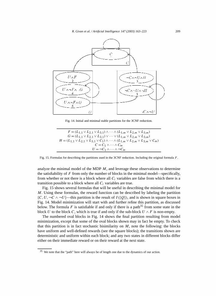
R. Givan et al. / Artificial Intelligence 147 (2003) 163–223 209
Fig. 14. Initial and minimal stable partitions for the 3CNF reduction.
F = (L1,1 ∨L2,1 ∨L3,1)∧ · · · ∧ (L1,m ∨L2,m ∨L3,m)
G= (L1,1 ∨L2,1 ∨L3,1)∨ · · · ∨ (L1,m ∨L2,m ∨L3,m)
H = (L1,1 ∨L2,1 ∨L3,1 ∨C1)∧ · · · ∧ (L1,m ∨L2,m ∨L3,m ∨Cm)
C = C1 ∧ · · · ∧Cm
U =¬C1 ∧ · · · ∧ ¬Cm
Fig. 15. Formulas for describing the partitions used in the 3CNF reduction. Including the original formula F .
analyze the minimal model of the MDP M , and leverage these observations to determinethe satisfiability of F from only the number of blocks in the minimal model—specifically,from whether or not there is a block where all Ci variables are false from which there is atransition possible to a block where all Ci variables are true.
Fig. 15 shows several formulas that will be useful in describing the minimal model forM . Using these formulas, the reward function can be described by labeling the partition{C,U,¬C ∧¬U}—this partition is the result of I ({Q}), and is shown in square boxes inFig. 14. Model minimization will start with and further refine this partition, as discussedbelow. The formula F is satisfiable if and only if there is a path35 from some state in theblock U to the block C, which is true if and only if the sub-block U ∧ F is non-empty.
The numbered oval blocks in Fig. 14 shows the final partition resulting from modelminimization, except that some of the oval blocks shown may in fact be empty. To checkthat this partition is in fact stochastic bisimilarity on M , note the following: the blockshave uniform and well-defined rewards (see the square blocks); the transitions shown aredeterministic and uniform within each block; and any two states in different blocks differeither on their immediate reward or on their reward at the next state.
35 We note that the “path” here will always be of length one due to the dynamics of our action.
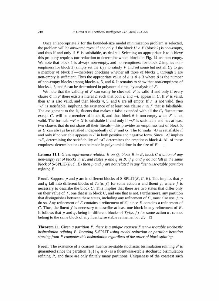
210 R. Givan et al. / Artificial Intelligence 147 (2003) 163–223
Once an appropriate k for the bounded-size model minimization problem is selected,
the problem will be answered “yes” if and only if the block U ∧F (block 2) is non-empty,and thus if and only if F is satisfiable, as desired. Selecting an appropriate k to achievethis property requires our reduction to determine which blocks in Fig. 14 are non-empty.We note that block 1 is always non-empty, and non-emptiness for block 2 implies non-emptiness for block 3 (simply set the Lj,i to satisfy F and set some but not all Cj to geta member of block 3)—therefore checking whether all three of blocks 1 through 3 arenon-empty is sufficient. Thus the appropriate value of k is β + 3 where β is the numberof non-empty blocks among blocks 4, 5, and 6. It remains to show that non-emptiness ofblocks 4, 5, and 6 can be determined in polynomial time, by analysis of F .We note that the validity of F can easily be checked: F is valid if and only if everyclause C in F there exists a literal L such that both L and ¬L appear in C. If F is valid,then H is also valid, and then blocks 4, 5, and 6 are all empty. If F is not valid, then¬F is satisfiable, implying the existence of at least one clause r in F that is falsifiable.The assignment to the Xi fluents that makes r false extended with all the Ci fluents trueexcept Cr will be a member of block 6, and thus block 6 is non-empty when F is notvalid. The formula ¬F ∧G is satisfiable if and only if ¬F is satisfiable and has at leasttwo clauses that do not share all their literals—this provides an emptiness test of block 5,as U can always be satisfied independently of F and G. The formula ¬G is satisfiable ifand only if no variable appears in F in both positive and negative form. Since ¬G implies¬F , determining the satisfiability of ¬G determines the emptiness block 4. All of theseemptiness determinations can be made in polynomial time in the size of F . ✷Lemma 11.1. Given equivalence relation E on Q, block B in E, block C a union of anynon-empty set of blocks in E, and states p and q in B , if p and q do not fall in the sameblock of S-SPLIT(B,C,E) then p and q are not related in any fluentwise-stable partitionrefining E.
Proof. Suppose p and q are in different blocks of S-SPLIT(B,C,E). This implies that pand q fall into different blocks of TF (α,f ) for some action α and fluent f , where f isnecessary to describe the block C. This implies that there are two states that differ onlyon their value of f , one that is in block C, and one that is not. Furthermore, any partitionthat distinguishes between these states, including any refinement of C, must also use f todo so. Any refinement of E contains a refinement of C, since E contains a refinement ofC. Thus, the fluent f is necessary to describe at least one block in any refinement of E.It follows that p and q , being in different blocks of TF (α,f ) for some action α, cannotbelong to the same block of any fluentwise stable refinement of E. ✷Theorem 11. Given a partition P , there is a unique coarsest fluentwise-stable stochasticbisimulation refining P . Iterating S-SPLIT using model reduction or partition iterationstarting from P computes this bisimulation regardless of the order of block splitting.
Proof. The existence of a coarsest fluentwise-stable stochastic bisimulation refining P isguaranteed since the partition {{q} | q ∈Q} is a fluentwise-stable stochastic bisimulationrefining P , and there are only finitely many partitions. Uniqueness of the coarsest such
R. Givan et al. / Artificial Intelligence 147 (2003) 163–223 211
partition is proven by contradiction. Assume two distinct partitions E1 and E2 are both
coarsest fluentwise-stable stochastic bisimulations refining P . Construct the new partitionE refining P that equates any two states equated by either E1 or E2, as follows: Eis the symmetric transitive closure of E1 union E2, where the partitions are viewedas equivalence relations represented as sets of pairs. We note that this partition E is acoarsening of both E1 and E2 and thus any fluent necessary to represent any block in E
must be necessary to represent at least one block E1 and at least one block in E2 (seeproof of Lemma 11.1). This ensures that any two states related by either E1 or E2 must bein the same block of TF (α,f ) for any fluent required to define a block of E—since anysuch fluent is required to define a block of E1 and a block of E2, and both E1 and E2 arefluentwise stable. Then a simple induction shows that since any two states related by E areconnected by a path made from E1/E2 arcs (i.e., a path of arcs drawn from E1 union E2),any two such states must be in the same block of TF (α,f ) for any fluent required to definea block of E. So E is fluentwise stable. Also, by Lemma 4.1 and Lemma 4.2, E must be astochastic bisimulation. Therefore, E is a fluentwise-stable, stochastic bisimulation that isa coarsening of both E1 and E2, contradicting our assumption.
That iterating S-SPLIT using model reduction or partition iteration finds the coarsestfluentwise stable stochastic bisimulation follows directly from Lemma 11.1. ✷Lemma 12.1. Given equivalence relation E on Q, block B in E, action α, and states p
and q in B , if p and q do not fall in the same block of FS-SPLIT(B,C,E), where C isthe union of any set of blocks in E, then p and q are not related in any fluentwise stablepartition refining E that is also fluentwise representable.
Proof. First we note that S-SPLIT(B,C,E) is a coarsening of the unique coarsestfluentwise-stable partitionE′ refining E (by Lemma 11.1). It follows that any fluent neededto represent S-SPLIT(B,C,E) is also needed to represent E′. FS-SPLIT(B,C,E) is thefluentwise partition given by the set of fluents required to represent S-SPLIT(B,C,E), andthus must be a coarsening of any fluentwise partition including all the fluents needed torepresent E′. But any representation of any fluentwise-stable partition refining E must useall the fluents needed in every representation of E′, since E′ is the coarsest such partition.So any fluentwise representation of a fluentwise-stable refinement of E must include allthe fluents used in FS-SPLIT(B,C,E), and thus must separate p and q , as desired. ✷Theorem 12. Given a partition P , there is a unique coarsest stochastic bisimulationrefining P even under the restriction that the partition be both fluentwise stable andfluentwise representable. Iterating FS-SPLIT using model reduction or partition iterationstarting from P computes this bisimulation regardless of the order of block splitting.
Proof. Let E be the unique coarsest fluentwise-stable stochastic bisimulation refiningP , which we know exists, by Theorem 11. The fluentwise-representable partition E′containing just those fluents required for representing E is a fluentwise-stable partitionthat is fluentwise representable—this follows because E′ refines E without requiring anynew fluents for representation. Since our choice of E guarantees that every fluentwise-stable partition refines E, every fluent needed to represent E is needed to represent
212 R. Givan et al. / Artificial Intelligence 147 (2003) 163–223
any fluentwise-stable partition; therefore all such fluents must be included in any
fluentwise representation of any fluentwise-stable partition. Thus E′ is a unique coarsestfluentwise stable stochastic bisimulation even under the restriction that it also be fluentwiserepresentable. That iterating FS-SPLIT, using either model reduction or partition iteration,yields this partition follows directly from Lemma 12.1. ✷Lemma 13.1. Suppose we are given an equivalence relation E on Q, where the blocks ofboth E and the partitions representing the factored MDP are represented as conjunctionsof literals. Then, any states p and q that do not fall in the same block of IR-SPLIT(E) arenot in the same block of any regression-stable partition refining E.Proof. Supposep and q fall into different blocks of IR-SPLIT(B,C,E). By the definition ofR-SPLIT, p and q must fall into different blocks of TF (α,f ) for some action α and fluentf necessary to describe some block C of E and either p or q must be in the regressionregion of C. Without loss of generality, let p be in the regression region of C. Consider aregression-stable refinement E′ of E—we show that p and q fall into different blocks ofE′. Since p is in the regression region of C,p must be in the regression region of some sub-block C′ of C in E′. Furthermore, because C is represented as a conjunction of literals,every fluent required to describe block C must be required to describe any sub-block ofC—in particular, the fluent f is required to describe the block C′. Now we have that pis in the regression region of C′, description of which requires the fluent f (for which p
and q fall into different blocks of TF (α,f )). It follows that p and q must be separatedby R-SPLIT(B ′,C′,E′) for any block B ′ of E′ containing both p and q; thus, there canbe no such B ′ in the regression-stable E′, and p and q fall into different blocks in E′, asdesired. ✷Theorem 13. Given a partition P , there exists a unique coarsest regression-stablestochastic bisimulation refining P .
Proof. The existence of a coarsest regression-stable stochastic bisimulation refining P isguaranteed since the partition {{q} | q ∈Q} is a regression-stable stochastic bisimulationrefining P , and there are only finitely many partitions. Suppose for contradiction that twodistinct partitions E1 and E2 are both coarsest regression-stable stochastic bisimulationsrefining P . Construct the new partition E refining P that equates any two states equated byeither E1 or E2, as follows: E is the symmetric transitive closure of E1 union E2, wherethe partitions are viewed as equivalence relations represented as sets of pairs. We note thatthis partition E is a coarsening of both E1 and E2 and thus any fluent necessary to representany block in E must be necessary to represent at least one block E1 and at least one blockin E2 (see proof of Lemma 11.1). This ensures that any two states related by either E1or E2 must be in the same block of TF (α,f ) for any fluent required to define any blockof E containing either state in its regression region—since any such fluent is required todefine such a block of E1 and such a block of E2 and both E1 and E2 are regression stable.But then a simple induction shows that since any two states related by E are connectedby a path of E1/E2 arcs, any two such states must be in the same block of TF (α,f )
for any fluent required to define any block of E containing either state in its regression
R. Givan et al. / Artificial Intelligence 147 (2003) 163–223 213
region. So E is regression stable. In addition, by Lemmas 4.1 and 4.2, E must also be a
stochastic bisimulation. Therefore, E is a regression-stable stochastic bisimulation that isa coarsening of both E1 and E2, which contradicts our assumption. ✷Lemma 14.1. Given a non-empty block B represented by a conjunction of literals Φ , eachfluent f is mentioned in Φ if and only if f appears in every formula describing B .Proof. (If) If f appears in every formula describing block B , then since Φ describes B,Φmust mention f .
(Only if) Since Φ describes a non-empty block B it follows that Φ is satisfiable. Letv be a truth assignment to all the fluents such that v satisfies Φ , and let v′ be v with thevalue of fluent f negated for some fluent f appearing in Φ . Since Φ describes B and isa conjunction of literals that mentions f , we know that v′ is not in block B . Furthermore,since both v and v′ satisfy all the same formulas that do not contain f , but B contains vand not v′, any description of B must contain f . ✷Lemma 14.2. If every block in a partition P is representable with a conjunction of literals,every block of IR-SPLIT(P ) is also so representable, under the assumption that the blocksin the partitions describing the MDP are also so representable.
Proof. Let C be a block of states. We define the “required fluents” of C, Req-Fluents(C),to be the set of fluents that are mentioned in every DNF block formula that describes blockC. We define Determines(C) to be the intersection of the TF partitions for each F ∈ Req-Fluents(C). Note that any partition of the form Determines(·) is made up only of blocksrepresentable by conjunctions of literals (given our assumptions about the MDP).
Let Regress(C) to be the partition Determines(C) modified so that any blocks B suchthat T (B,α,C)= 0 for every action α are aggregated into a single block. Let S be a set ofblocks. We use Determines(S) and Regress(S) to denote the intersection over members e ofS of Determines(e) and Regress(e), respectively. Let s be a state. We define Reachable(s)to be the set of blocks C of P such that T (s,α,C) �= 0. For any block B , let Reachable(B)is the set of all blocks C such that some state s in B has T (s,α,C) �= 0. We prove thatRegress(P ) intersected with P and R is the same partition as IR-SPLIT(P ), and that everyblock B of Regress(P ) is an element of Determines(Reachable(B)). Thus, any block ofIR-SPLIT(P ) can be represented as a conjunction of literals, since it is the intersection ofblocks from P,R, and a Determines(·) partition, where each block is representable as aconjunction of literals.
We now show that Regress(P ) intersected with P and R is the same partition asIR-SPLIT(P ). Let s and t be states from the same block of Regress(P ) ∩ P ∩ R. Sinces and t are in the same block of P , to be in different blocks of IR-SPLIT(P ) they must fallin different blocks of some call to R-SPLIT(B ′,C,P ) for some C in P where s and t areboth in B ′. States s and t are in different blocks of R-SPLIT(B ′,C,P ) only if either sand t have different reward or are in different blocks of TF for some F in Req-Fluents(C)and either s or t has a non-zero probability of transitioning to C. Since s and t are in thesame block of R they must have the same reward, and since they are in the same block ofRegress(C) they must either both have zero probability of transition to C or be in the same
214 R. Givan et al. / Artificial Intelligence 147 (2003) 163–223
block of TF for all F in Req-Fluents(C). So, s and t are in the same block of IR-SPLIT(P ),
and thus that Regress(P ) intersected with P and R refines IR-SPLIT(P ).Now consider s and t from the same block B of IR-SPLIT(P ). Since IR-SPLIT(P ) alwaysrefines both P and R, s and t must be the same blocks of P and R. We know that block B
is not split by any call of the form R-SPLIT(B,C,P ) for any C ∈ P , implying that eitherT (B,α,C) = 0 for all α or every state in B falls in the same block of T F for all F inReq-Fluents(C). Since s and t are both in B , they must be in the same block of Regress(C)for any C ∈ P , and therefore in the same block of Regress(P ), Being in the same blocks ofthe partitions Regress(P ),P , and R means s and t are in the same block of the intersectionof those partitions and thus IR-SPLIT(P ) refines Regress(P ) intersected with P and R.Since Regress(P ) intersected with P and R refines IR-SPLIT(P ) and IR-SPLIT(P ) refinesRegress(P ) intersected with P and R they must be the same partition.
It remains to show that any block B of Regress(P ) is an element of Determines(Reach-able(B)). Consider states s and t in B of Regress(P ). For all blocks C of P, s and t arein the same block of Regress(C). So, by definition of Regress(C), whenever T (B,α,C) >0, s and t are in the same block of Determines(C). The set of blocks C from P whereT (B,α,C) > 0 is just Reachable(B), so s and t are in the same block, called B ′, ofDetermines(Reachable(B)). So, block B refines a block of Determines(Reachable(B)).
We now consider state s′ ∈ B ′ and show that s′ ∈ B , to conclude that B ′ = B ,completing our proof. We consider any state s in B , and show that s and s′ fall into the sameblock of Regress(C) for every block C of P . It suffices to show that Reachable(s) equalsReachable(s′) and that s and s′ fall into the same block of TF for any F in Req-Fluents(C)for C in Reachable(s). Consider C in Reachable(s). Note that any such C is a member ofReachable(B) and our choice of B ′ as the block of Determines(Reachable(B)) containingB implies that s′ and s are in the same block of TF for all fluents in Req-Fluents(C). Itremains to show that Reachable(s) equals Reachable(s′).
As just argued, s and s′ fall into the same block of TF for any fluent F in Req-Fluents(C)for any C in Reachable(s). This implies that Reachable(s) is a subset of Reachable(s′).The fact that Reachable(s′) is a subset of Reachable(s) can be argued as follows. As justshown, s and s′ fall in the same block of TF for any F in Req-Fluents(C) for any C inReachable(B). This implies that the transition probability from s or s′ to any such C isthe same. But since these probabilities must sum to one (because s can only reach blocksC that are reachable from B , as s is in B), s′ cannot transition to any block C′ not inReachable(B), and hence Reachable(s′) is a subset of Reachable(s), as desired. ✷Theorem 14. Let M be a factored MDP with all partition blocks represented asconjunctions of literals. Given a starting partition P also so represented, iteratingR-SPLIT using partition iteration computes the coarsest regression-stable stochasticbisimulation refining P , regardless of the order in which blocks are selected for splitting.
Proof. Lemma 14.2 implies that every block in the partition resulting from the applicationof the IR-SPLIT operation has a formula that is a conjunction of literals. Lemma 13.1 thenimplies that iterating IR-SPLIT using partition iteration returns the coarsest regression-stablestochastic bisimulation, which by Theorem 13 is unique. ✷
R. Givan et al. / Artificial Intelligence 147 (2003) 163–223 215
Lemma 15.1. Given a fluentwise partition P and a minimal tree-represented factored MDP
M , the partition computed by Add-relevant(P ) is the partition IFS-SPLIT(P ).Proof. Let P ′ be the fluentwise partition returned by Add-relevant. Partition P ′ isfluentwise representable. Also, P ′ is a refinement of P since P ′ (as a set of fluents) containsP . We define fluentwise stability with respect to a partition to mean fluentwise stabilitywith respect to every block of that partition. Below we show that any fluentwise partitionomitting any fluent in P ′ is not fluentwise stable with respect to P , and that P ′ is fluentwisestable with respect to P . Thus, P ′ is the coarsest fluentwise-representable partition refiningP that is fluentwise stable with respect to P , i.e., IFS-SPLIT(P ), as desired.
For a partition to be fluentwise stable with respect to a fluent means that every pairof states in the same block of the partition must have the same probability distributionover that fluent for every action. If a fluent f ′ is tested in a minimal tree representationof the effect of some action α on some fluent f then any fluentwise partition omitting f ′is not fluentwise stable with respect to f ; two states differing only on f ′ must differ intheir probability of setting f when taking α. To be fluentwise stable with respect to P , apartition must be stable with respect to all the fluents in P (as a set of fluents), becausedescribing any block in P with a formula requires all fluents in P . It follows that Add-relevant constructs P ′ by adding to P only those fluents that cannot be omitted from apartition that is fluentwise stable with respect to P , as desired.
The independence assumptions implicit in the factored representation of the MDP M
ensure that any fluent f ′ not mentioned in the tree for action α and fluent f has no effecton the probability of setting f when taking α. Specifically, states differing only on f ′ havethe same probability of setting f when taking α. Partition P ′ contains every fluent in anytree defining the effect of any action on any fluent in P , so that two states in the same blockcan only differ on fluents not mentioned in any such tree. It follows that any two states inthe same block of P ′ have the same probability of setting any fluent in P , and thus that P ′is fluentwise stable with respect to P . ✷Theorem 15. Given a minimal tree-represented MDP, model reduction using FS-SPLITyields the same partition that state-space abstraction yields, and does so in polynomial-time in the MDP representation size.
Proof. Since state space abstraction iterates Add-relevant starting with the fluentwisepartition Fluents(R) until convergence, it follows directly from 0 that state-spaceabstraction and iterating FS-SPLIT starting with Fluents(R) find the same partition.A simple analysis of partition iteration shows that the first iteration returns Fluents(R)when using FS-SPLIT. Theorem 12 then implies that model reduction using FS-SPLITand state space abstraction yield the same partition.
We now show the polynomial-time complexity claim. To obtain this complexity,the basic method must be optimized to make only the linearly many FS-SPLIT callsdescribed below, avoiding unnecessary calls, as follows. When the partition P is fluentwiserepresented, the partition P ′ = FS-SPLIT(B,C,P ) does not depend on the choice of Bor C from P because the same set of fluents are used in every block formula. Thus, P ′will not be further split by calls of the form FS-SPLIT(B ′,C,P ′), where B ′ is a block of
216 R. Givan et al. / Artificial Intelligence 147 (2003) 163–223
P ′ and C is a block of P . This observation implies that partition iteration can compute
IFS-SPLIT(P ) with only one call to FS-SPLIT(B,C,P ), using any blocks B and C in thepartition P . We further note that each call to FS-SPLIT increases the number of fluentsin the partition representation, except the last call, which does not change the partition.Thus only linearly many calls to FS-SPLIT can be made during partition iteration. We canconclude that partition iteration terminates in polynomial time, by showing that each callto FS-SPLIT terminates in polynomial time.Consider the call FS-SPLIT(B,C,P ), where B and C are blocks of P , and P is afluentwise-represented partition. Every fluent in the set defining P is present in every DNFformula defining any block of P . So, for any choice of B and C, the resulting partitionmust be fluentwise partition represented by the set of fluents that appear anywhere in thetrees defining the effects of the actions on fluents in P , together with any fluents in P orappearing in the tree defining R. This set is computable in time polynomial in the size ofthose trees plus the number of fluents in P . ✷Lemma 16.1. Let V be a tree-represented value function, where PV is the partition givenby the tree. Let α be an action, and for any block C of PV , let ΦC denote the conjunctionof literals describing C. We then have the following:
The partition computed by PRegress(V ,α) is the intersection over all blocks C of PV
of Regression-determining(ΦC,α).
Proof. We use induction on the depth of the tree for V . As the base case suppose V is aleaf node. Here, PRegress returns the partition {Q}, and Regression-determining(true, α)also returns {Q}. In the inductive case, let fluent f be the fluent tested at the root of thetree, and assume the lemma for the sub-trees. Let P∩ be the intersection over all blocksC ∈ PV of Regression-determining(ΦC,α). We show that P∩ is PRegress(V,α).
We start by noting that the partition returned by PRegress(V,α) is built by refiningTF (α,f ) using Replace. Since f is at the root of V .Tree every formula describingany block C of PV includes f . In particular, the conjunction describing any blockof V must contain f , since it is on every path from the root of V to a leaf, andso f must be in Fluents(ΦC )fp. Thus for every block C of PV the call to Partition-determining(Fluents(ΦC),α) must be fluentwise stable with respect to f , since all statesin the same block of Partition-determining(Fluents(ΦC),α) must be in the same blockof TF (α,f ′) for any fluent f ′ in Fluents(ΦC ). Consider the partition variable PC in thepseudo-code for Regression-determining(ΦC,α), after it is assigned. Since every blockin PC is a block from Partition-determining(Fluents(ΦC),α), any such block must befluentwise stable with respect to f . We note that the union of all blocks in PC is theregression region for C, as defined in Section 4.6. It follows that every state in theregression region for a block C is in a fluentwise-stable block (with respect to f ) in thepartition Regression-determining(ΦC,α), and thus in any partition refining this partition.Every state must be carried to some state under action α, so every state is in the regressionregion for some block of PV . So P∩ must be fluentwise stable with respect to f ; so P∩refines TF (α,f ).
We now analyze the refinement of TF (α,f ) returned by PRegress and show that thisrefinement is the same as the refinement of TF (α,f ) by P∩. PRegress(V,α) is computed
R. Givan et al. / Artificial Intelligence 147 (2003) 163–223 217
by replacing each block B of TF (α,f ) with the intersection of all the partitions resulting
from relevant recursive calls to PRegress, restricted to block B . A recursive call on animmediate sub-tree of V is relevant to block B if the value of f leading to that sub-treehas a non-zero probability after taking action α in block B (this probability is uniformthroughout B). By the induction hypothesis, each sub-tree partition is the intersectionof Regression-determining(ΦC ′, α) for all blocks C′ of the partition represented by thesub-tree. Each such block C′ becomes a block C of PV when restricted to the value off determining the branch for the sub-tree containing C′—the formula ΦC will be ΦC ′conjoined with the appropriate literal for f . The refinement of B in PRegress(V,α) istherefore the intersection of Regression-determining(ΦC ′, α) for all the blocks C′ of allsub-trees relevant to B , restricted to B .Consider a block B of TF (α,f ) and two states i and j from B in different blocks ofPRegress(V , α). Our analysis of PRegress(V,α) just above implies that i and j must bein different blocks of Regression-determining(ΦC ′, α) for some block C′ of a sub-tree ofV relevant to B . Let C be the block formed by restricting C′ to the relevant value of f .Any state in B has a non-zero block transition probability to C′ if and only if that statealso has a non-zero block transition probability to C— his follows from the definition of“relevant”. From this, one can show that i and j are also in different blocks of Regression-determining(ΦC,α). It follows that P∩ refines PRegress(V,α).
Now consider a block C of PV and the corresponding formula ΦC , and any two statesi and j in the same block of PRegress(V , α). For any fluent f ′ in ΦC , we have eitherthat ΦC is always false after performing α whether starting from i or from j , or that bothstates have an equal probability of transitioning to a state where f ′ is true after performingα. This implies that states i and j are either both in block Q0 or both in block of PC ,respectively, in the pseudo-code for Regression-determining(ΦC,α). We conclude thatany two states in the same block of PRegress(V,α) must also be in the same block ofRegression-determining(ΦC,α) for any block C of PV —thus PRegress(V,α) must refineP∩. Since PRegress(V,α) and P∩ refine each other, they must be equal, as desired. ✷Lemma 16.2. Given action α and value function V , Regress-action(V ,α) on MDP M
intersected with V .tree gives the partition computed by IR-SPLIT(V .Tree) on MDP Mπα .
Proof. We say that a partition P ′ is a regression of P for MDP M if P ′ = R-SPLIT(B,C,P ′) for any blocks B of P ′ and C of P , where R-SPLIT is computed relativeto M . It is not hard to show that the coarsest regression of P refining P for any M isIR-SPLIT(P ) for M . Let P be the partition V .Tree, and let P ′ be P∩ Regress-action(V,α)on MDP M . We show that P ′ is the coarsest regression of P refining P for Mπα , toconclude that P ′ = IR-SPLIT(P ) relative to Mπα .
Since P ′ is formed by intersection with P,P ′ refines P . We show that P ′ is a regressionof P relative to Mπα . Let i and j be any two states in the same block B of P ′. Then weneed to show that i and j are in the same block of R-SPLIT(B,C,P ′) relative to Mπα
for any block C of P . We note that Regress-Action(V,α) uses partition intersection withthe reward partition to return a partition that refines the R partition. Thus, the states i
and j must have the same reward. States i and j must also belong to the same blockof Regression-determining(ΦC,α) for any block C of P by Lemma 16.1 since Regress-

218 R. Givan et al. / Artificial Intelligence 147 (2003) 163–223
action(V,α) returns a refinement of PRegress(V,α). We can then see that states i and j
must belong to the same block of Block-split(B,C,α) (as computed by the code of Fig. 7with Partition-determining replaced by Regression-determining to compute R-SPLIT, asdiscussed in Section 4.6)—and thus to the same block of R-SPLIT(B,C,P ′) for Mπα , asdesired. It follows that P ′ is a regression of P for Mπα .
We now argue that P ′ is the coarsest regression of P for Mπα . Suppose not, and considersuch coarser regression P ′′, and consider states i and j in the same block of P ′′ but indifferent blocks of P ′. Note, based on the pseudo-code for Regress-action in Fig. 11, thatif i and j are in different blocks of P ′ then they must either be in different blocks ofP , have different rewards, or (using Lemma 16.1) be in different blocks of Regression-determining(ΦC,α) for some block C of P . In each of these cases, we can show thatthe block B of P ′′ containing i and j is split to separate i and j into different blocks ofR-SPLIT(B,C,P ′) for some block C of P , contradicting our assumption about P ′′. ✷Lemma 16.3. Given policy π and value function V , Regress-policy(V ,π) on MDP M
intersected with V .tree gives the partition computed by IR-SPLIT(V .Tree) on MDP Mπ
intersected with π.Tree.
Proof. Regress-policy(V,π ) returns the partition that refines π .Tree by intersecting eachblock b of π .Tree with Regress-action(V,αb) where αb is the action labeling block b, i.e.,π .Label(b). Let M ′ be the MDP M extended by adding a new action α′ defined to so thatfor each state s,α′ behaves identically to π(s) in M . Then Regress-policy(V,π ) in M
gives the same partition as Regress-action(V,α′) in M ′ intersected with π .Tree. ApplyingLemma 16.2 gives that Regress-policy(V,π ) intersected with V .tree is the same partitionas IR-SPLIT(V .Tree) for MDP M ′
Πα′ intersected with π .Tree. To complete the proof, we
note that M ′Πα′ =Mπ by the construction of α′ and Mπ . ✷
Lemma 16.4. Given tree-represented value functions V1 and V2, with correspondingpartitions V1.Tree refining V2.Tree, we have all of the following monotonicity properties:
(1) PRegress(V1, α) refines PRegress(V2, α) for any action α,(2) Regress-action(V1, α) refines Regress-action(V2, α) for any action α,(3) Regress-policy(V1,π) refines Regress-policy(V2,π) for any policy π , and(4) IR-SPLIT(V1.Tree) refines IR-SPLIT(V2.Tree).
Proof. We first show some properties of PRegress and of partitions represented as treesthat will be useful for proving that PRegress(V1, α) refines PRegress(V2, α) for any actionα. It follows from Lemma 16.1 that the partition returned by PRegress(V,α) for a tree-represented value function V depends on only the blocks of V .Tree and not on the structureof the tree itself. Another useful property is that for any value function V ′ which refinesV , both represented as trees, we can change the structure of V ′ to have the same rootvariable as V without changing the represented partition. We will prove this property byconstruction. Let X be the root variable of V .Tree, we first note that X must be used todescribe any block of V ′.Tree because of the following three facts. (1) Every block formulafor any block of V .Tree or V ′.Tree is a conjunction of literals. (2) Every block of V .Tree
R. Givan et al. / Artificial Intelligence 147 (2003) 163–223 219
mentions X. (3) Every block of V ′.Tree is a sub-block of a block of V .Tree. For each
value x of X, let the tree τx be the tree V ′.Tree, with every sub-tree that has root variableX replaced by the immediate sub-tree of that sub-tree corresponding to x . Now construct atree τ with the root node labeled with X, and the sub-tree for each value x of X being τx .Noting that X must occur on every root-to-leaf path in V ′.Tree, it is easy to show that theτ represents the same partition as V ′.Tree, but has the same root variable as V .Tree.We now prove by induction on the height of V2.Tree that PRegress(V1, α) refinesPRegress(V2, α) for any action α. For the base case, consider a value function V2 consistingof a single leaf node. In this case PRegress(V2, α) returns {Q}, which is refined by everypartition so the property is trivially true. In the inductive case, first modify V1.Tree sothat it has the same root variable as V2.Tree without changing the partition represented,as just described in the previous paragraph. Examining the pseudo-code for PRegress,given in Fig. 11, we note that the same X is selected by the calls PRegress(V1, α) andPRegress(V2, α) for any action α, and therefore the assignment Px.Tree = Px|α .Treeassigns the same starting tree for both calls. We now observe that Subtree(V1, x) refinesSubtree(V2, x) for every value x of X, since V1 refines V2, and that the height ofSubtree(V2, x) is less than the height of V2.Tree. Therefore, by the induction hypothesiswe have that every Pxi in the call PRegress(V1, α) refines the corresponding Pxi in the callPRegress(V2, α).
Let T1 be the T calculated to replace block B of Px .Tree in the call PRegress(V1, α)and let T2 be the T calculated to replace B in the call PRegress(V2, α). We now show thatT1 refines T2. For states p and q to be in the same block of T1 they must be in the sameblock of Pxi in the call PRegress(V1, α) for each xi such that Pr(X = xi) in the distributionPx|a .Label(B) is greater than zero. Therefore, since Pxi in the call PRegress(V1, α) refinesthe corresponding Pxi in the call PRegress(V2, α),p and q must be in the same blockof Pxi in the call PRegress(V2, α) for each xi such that Pr(X = xi) in the distributionPx|a .Label(B) is greater than zero. Since these Pxi are intersected to obtain T2,p and q
must be in the same block of T2 proving that T1 refines T2 when replacing any block B .Part (1) of the lemma follows. The second and third parts of the lemma follow directlyfrom the first and second, respectively, along with an examination of the pseudo-code inFig. 11 and basic properties of intersection on partitions relative to the partition refinementrelation.
To prove the last part of the lemma, that IR-SPLIT(V1.Tree) refines IR-SPLIT(V2.Tree), weshow that any two states in the same block of IR-SPLIT(V1.Tree) are in the same block ofIR-SPLIT(V2.Tree). Let p and q be two states from the same block B1 of IR-SPLIT(V1.Tree).This means that p and q must be in the same block of V1.Tree and in the same block ofR-SPLIT(B1,B
′1, IR-SPLIT(V1.Tree)) for any block B ′1 of V1.Tree.
In order to show that p and q are in the same block of IR-SPLIT(V2.Tree) we show thatthey are in the same block of V2.Tree and in the same block of R-SPLIT(B2,B
′2,P ) for any
block B ′2 of V2.Tree, any block B2 containing both p and q , and any partition P containingblock B2. Since V1.Tree refines V2.Tree, the fact that p and q are in the same block ofV1.Tree directly implies that they are in the same block of V2.Tree. For any B ′2 ∈ V2.Tree,consider the set β of blocks {B ′1 | B ′1 ∈ V1.Tree, B ′1 ⊆ B ′2}. Note that since p and q arein the same block of IR-SPLIT(V1.Tree), they must agree on the probability of transition toany block in V1.Tree. Let p and q both be in block B2 and B2 be a block of partition P . If
220 R. Givan et al. / Artificial Intelligence 147 (2003) 163–223
for every member B ′ of β , the probability of transitioning from both p and q to B ′ under
1 1an action α is zero, then p and q are in the same block of R-SPLIT(B2,B′2,P ) since their
probabilities of transitioning to B ′2 are both zero and thus. Now consider for some memberB ′1 of the set, the probability of transitioning from either p or q to B ′1 is non-zero undersome action α. Then, since p and q are in the same block of IR-SPLIT(V1.Tree), they mustbe in the same block of TF (α,f ) for every fluent f needed to describe block B ′1. SinceB ′1 is a sub-block of B ′2 and both B ′1 and B ′2 can be represented as a conjunction of literalsevery fluent needed for B ′2 is needed for B ′1. Therefore, p and q must be in the same blockof TF (α,f ) for every fluent f needed to describe block B ′2 and thus be in the same blockof R-SPLIT(B2,B
′2,P ). Using one of these two cases for each action, we get that p and q
are in the same block of R-SPLIT(B,B ′2,P ), whenever p and q are both in block B and B
is in P . ✷Theorem 16. For any tree-represented MDP M and policy π , SSA(π) produces the sameresulting partition as partition iteration on Mπ using R-SPLIT starting from the partitionπ .Tree.
Proof. We first show that SSA(π ) and partition iteration of Mπ using R-SPLIT, startingfrom the partition π .Tree, written PIR-SPLIT(π .Tree, Mπ ), compute the same partition. Wenotate the sequence of partitions produced by partition iteration as follows: P0 = π .Tree,and Pi+1 = IR-SPLIT(Pi). The partition PIR-SPLIT(π .Tree, Mπ ) equals Pm, for all m greaterthan the number tP of iterations to convergence. Likewise, denote the sequence of factoredvalue functions produced by SSA as follows: V0 = R, and Vi+1 = Regress-policy(Vi,π ).Likewise, the partition SSA(π ) equals Vm, for all m greater than the number tV of iterationsto convergence. By induction on the number n of iterations of partition iteration, we showthat Vn+1.Tree refines Pn and Pn+1 refines Vn.Tree, for all n > 0, and conclude thatSSA(π ).Tree equals MRR-SPLIT(π .Tree, Mπ ), as desired, by considering n > max(tP , tV ).
For the base case, consider n equal to 1. Since, by inspection, Regress-policy(·,π ).Treealways refines the partition π .Tree, for any policy π , we know that V1.Tree refines P0.Likewise, since, by inspection, the partition IR-SPLIT(P ) always refines the reward partitionR.Tree, for any partition P , we know that P1 refines V0.Tree. For the inductive case, wefirst show that Pn+1 refines Vn.Tree. By a nested induction on n, we can show that Pn+1refines P0, using the fact that IR-SPLIT(P ) refines P , for any P . Thus,
Pn+1 = Pn+1 ∩ P0 = IR-SPLIT(Pn)∩ π.Tree. (A.1)
But Pn refines Vn−1 by the induction hypothesis, so Lemma 16.4 implies that IR-SPLIT(Pn)
refines IR-SPLIT(Vn−1). Together with Eq. (A.1), this implies that Pn+1 refinesIR-SPLIT(Vn−1) ∩ π .Tree. By applying Lemma 16.3, we derive that Pn+1 refines Regress-policy(Vn−1,π)∩Vn−1.Tree, which is just Vn ∩Vn−1, by definition. It is straightforward toshow by a nested induction on n that Vn refines Vn−1, using Lemma 16.4, so we concludethat Pn+1 refines Vn.
That Vn+1.Tree refines Pn is proven similarly: first, Vn+1 = Vn+1 ∩ Vn = Regress-policy(Vn,π) ∩ Vn. Applying Lemma 16.3, we have Vn+1 = IR-SPLIT(Vn) ∩ π .Tree. ButVn refines Pn−1 by the induction hypothesis, so Lemma 16.4 implies that IR-SPLIT(Vn)
refines IR-SPLIT(Pn−1). With Vn+1 = IR-SPLIT(Vn) ∩ π .Tree, we have that Vn+1 refines
R. Givan et al. / Artificial Intelligence 147 (2003) 163–223 221
IR-SPLIT(Pn−1) ∩ π .Tree, which is just Pn since IR-SPLIT(Pn−1) ∩ π.Tree = Pn ∩ P0 =
Pn. ✷Theorem 17. The policy improvement “for” loop in SPI computes IR-SPLIT(Vπ .Tree).Proof. Let b be a block in π .Tree. We note that Vπ in SPI is a factored value functioncomputed by SSA, and so Vπ must be a fixed-point of Regress-policy(·,π ). This impliesthat Vπ .Tree must refine π .Tree, and, by examining the Regress-policy pseudo-code, thatblocks b′ in Vπ that refine b are also in Regress-action(Vπ,π(b)). Combine these to getthat Regress-action(Vπ,π(b)) refines {¬b} ∪ {b′ | b′ ∈ Vπ ∧ b′ ⊆ b}. We also have⋂
α∈ARegress-action(Vπ,α) refines π .Tree∩ Vπ .Tree, (A.2)
since b was arbitrary. Given that partition intersection is associative and commutative, thepolicy improvement “for” loop in SPI can be seen to iterate over the actions to compute
π .Tree ∩ ⋂α∈A
Regress-action(Vπ,α).Tree.
Eq. (A.2) then implies that the computed partition is⋂α∈A
(Regress-action(Vπ,α)∩ Vπ .Tree
),
which is⋂α∈A
IR-SPLIT(Vπ .Tree) in Mπα , (A.3)
by applying Lemma 16.2 to each of the partitions in the intersection. It is possible to showthat for value function V and MDP M ′ with action space A′,
IR-SPLIT(V ) in MDP M ′
=⋂α∈A′
⋃B∈V .Tree
⋂C∈V .Tree
Block-split(B,C,α) in M ′, (A.4)
where the intersections are partition intersections,36 and the union is a simple set union,treating the partitions as sets of blocks (the union combines partitions of disjoint sets toget a partition of the union of those disjoint sets). Applying this to each of the terms in theintersection in Eq. (A.3), noting that the only action available in Mπα is α yields⋂
α∈A
⋂α′∈{α}
⋃B∈Vπ.Tree
⋂C∈Vπ.Tree
Block-split(B,C,α′) in Mπα
for the partition. Simplifying and noting Block-split(B,C,α) is the same in Mπα and M ,⋂α∈A
⋃B∈Vπ.Tree
⋂C∈Vπ.Tree
Block-split(B,C,α) in M (A.5)
is the computed partition. Finally, applying Eq. (A.4) gives IR-SPLIT(Vπ .Tree) in M . ✷36 The resulting partition has a block for each pair of blocks in the partitions being intersected, representing the
intersection of those two blocks, with empty blocks in the result removed.
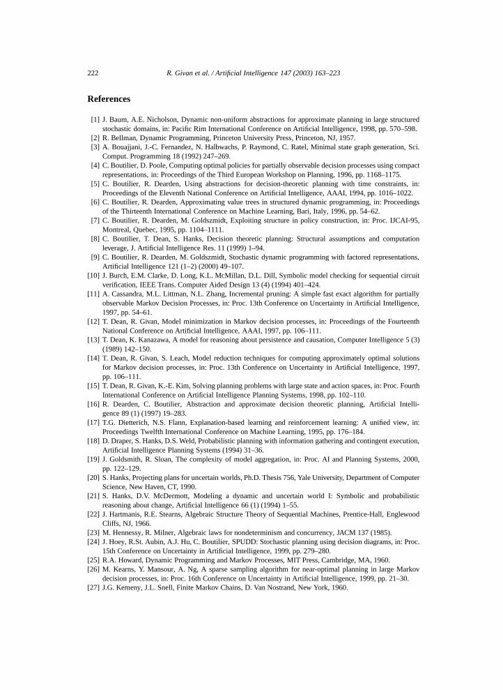
222 R. Givan et al. / Artificial Intelligence 147 (2003) 163–223
References
[1] J. Baum, A.E. Nicholson, Dynamic non-uniform abstractions for approximate planning in large structuredstochastic domains, in: Pacific Rim International Conference on Artificial Intelligence, 1998, pp. 570–598.
[2] R. Bellman, Dynamic Programming, Princeton University Press, Princeton, NJ, 1957.[3] A. Bouajjani, J.-C. Fernandez, N. Halbwachs, P. Raymond, C. Ratel, Minimal state graph generation, Sci.
Comput. Programming 18 (1992) 247–269.[4] C. Boutilier, D. Poole, Computing optimal policies for partially observable decision processes using compact
representations, in: Proceedings of the Third European Workshop on Planning, 1996, pp. 1168–1175.[5] C. Boutilier, R. Dearden, Using abstractions for decision-theoretic planning with time constraints, in:
Proceedings of the Eleventh National Conference on Artificial Intelligence, AAAI, 1994, pp. 1016–1022.[6] C. Boutilier, R. Dearden, Approximating value trees in structured dynamic programming, in: Proceedings
of the Thirteenth International Conference on Machine Learning, Bari, Italy, 1996, pp. 54–62.[7] C. Boutilier, R. Dearden, M. Goldszmidt, Exploiting structure in policy construction, in: Proc. IJCAI-95,
Montreal, Quebec, 1995, pp. 1104–1111.[8] C. Boutilier, T. Dean, S. Hanks, Decision theoretic planning: Structural assumptions and computation
leverage, J. Artificial Intelligence Res. 11 (1999) 1–94.[9] C. Boutilier, R. Dearden, M. Goldszmidt, Stochastic dynamic programming with factored representations,
Artificial Intelligence 121 (1–2) (2000) 49–107.[10] J. Burch, E.M. Clarke, D. Long, K.L. McMillan, D.L. Dill, Symbolic model checking for sequential circuit
verification, IEEE Trans. Computer Aided Design 13 (4) (1994) 401–424.[11] A. Cassandra, M.L. Littman, N.L. Zhang, Incremental pruning: A simple fast exact algorithm for partially
observable Markov Decision Processes, in: Proc. 13th Conference on Uncertainty in Artificial Intelligence,1997, pp. 54–61.
[12] T. Dean, R. Givan, Model minimization in Markov decision processes, in: Proceedings of the FourteenthNational Conference on Artificial Intelligence, AAAI, 1997, pp. 106–111.
[13] T. Dean, K. Kanazawa, A model for reasoning about persistence and causation, Computer Intelligence 5 (3)(1989) 142–150.
[14] T. Dean, R. Givan, S. Leach, Model reduction techniques for computing approximately optimal solutionsfor Markov decision processes, in: Proc. 13th Conference on Uncertainty in Artificial Intelligence, 1997,pp. 106–111.
[15] T. Dean, R. Givan, K.-E. Kim, Solving planning problems with large state and action spaces, in: Proc. FourthInternational Conference on Artificial Intelligence Planning Systems, 1998, pp. 102–110.
[16] R. Dearden, C. Boutilier, Abstraction and approximate decision theoretic planning, Artificial Intelli-gence 89 (1) (1997) 19–283.
[17] T.G. Dietterich, N.S. Flann, Explanation-based learning and reinforcement learning: A unified view, in:Proceedings Twelfth International Conference on Machine Learning, 1995, pp. 176–184.
[18] D. Draper, S. Hanks, D.S. Weld, Probabilistic planning with information gathering and contingent execution,Artificial Intelligence Planning Systems (1994) 31–36.
[19] J. Goldsmith, R. Sloan, The complexity of model aggregation, in: Proc. AI and Planning Systems, 2000,pp. 122–129.
[20] S. Hanks, Projecting plans for uncertain worlds, Ph.D. Thesis 756, Yale University, Department of ComputerScience, New Haven, CT, 1990.
[21] S. Hanks, D.V. McDermott, Modeling a dynamic and uncertain world I: Symbolic and probabilisticreasoning about change, Artificial Intelligence 66 (1) (1994) 1–55.
[22] J. Hartmanis, R.E. Stearns, Algebraic Structure Theory of Sequential Machines, Prentice-Hall, EnglewoodCliffs, NJ, 1966.
[23] M. Hennessy, R. Milner, Algebraic laws for nondeterminism and concurrency, JACM 137 (1985).[24] J. Hoey, R.St. Aubin, A.J. Hu, C. Boutilier, SPUDD: Stochastic planning using decision diagrams, in: Proc.
15th Conference on Uncertainty in Artificial Intelligence, 1999, pp. 279–280.[25] R.A. Howard, Dynamic Programming and Markov Processes, MIT Press, Cambridge, MA, 1960.[26] M. Kearns, Y. Mansour, A. Ng, A sparse sampling algorithm for near-optimal planning in large Markov
decision processes, in: Proc. 16th Conference on Uncertainty in Artificial Intelligence, 1999, pp. 21–30.[27] J.G. Kemeny, J.L. Snell, Finite Markov Chains, D. Van Nostrand, New York, 1960.
R. Givan et al. / Artificial Intelligence 147 (2003) 163–223 223
[28] D. Koller, R. Parr, Policy iteration for factored MDPs, in: Proc. 16th Conference on Uncertainty in Artificial
Intelligence, 2000, pp. 326–334.[29] N. Kushmerick, S. Hanks, D. Weld, An algorithm for probabilistic planning, Artificial Intelligence 76 (1–2)(1995).
[30] K.G. Larsen, A. Skou, Bisimulation through probabilistic testing, Inform. and Comput. 94 (1) (1991) 128.[31] D. Lee, M. Yannakakis, Online minimization of transition systems, in: Proceedings of 24th Annual ACM
Symposium on the Theory of Computing, 1992.[32] S.-H. Lin, T. Dean, Generating optimal policies for high-level plans with conditional branches and loops, in:
Proceedings of the Third European Workshop on Planning, 1995, pp. 205–218.[33] M. Littman, The Witness algorithm: Solving partially observable Markov decision processes, Brown
University, Department of Computer Science, Technical Report CS-94-40, 1994.[34] M. Littman, T. Dean, L. Kaelbling, On the complexity of solving Markov decision problems, in: Proc.
Eleventh Conference on Uncertainty in Artificial Intelligence, 1995, pp. 394–402.[35] M. Littman, Probabilistic propositional planning: Representations and complexity, in: Proceedings of the
Fourteenth National Conference on Artificial Intelligence, 1997, pp. 748–754.[36] D. McAllester, D. Rosenblitt, Systematic nonlinear planning, in: Proceedings of the Eighth National
Conference on Artificial Intelligence, 1991, pp. 634–639.[37] R. Milner, Communication and Concurrency, in: Series in Computer Science, Prentice-Hall International,
1989.[38] R. Milner, Operational and algebraic semantics of concurrent processes, in: J. van Leeuwen (Ed.), Handbook
on Theoretical Computer Science, Elsevier Science, Amsterdam, 1990, pp. 1201–1242.[39] G.E. Monahan, A survey of partially observable Markov decision processes: Theory models and algorithms,
Management Sci. 28 (1) (1982) 1–16.[40] D.M. Park, Concurrency on automata and infinite sequences, in: P. Deussen (Ed.), Conference on Theoretical
Computer Science, in: Lecture Notes in Computer Science, Vol. 104, Springer, Berlin, 1981.[41] J. Pearl, Probabilistic Reasoning in Intelligent Systems: Networks of Plausible Inference, Morgan
Kaufmann, San Francisco, CA, 1988.[42] M.L. Puterman, Markov Decision Processes, Wiley, New York, 1994.[43] N.L. Zhang, W. Zhang, Speeding up the convergence of value iteration in partially observable Markov
decision processes, J. Artificial Intelligence Res. 14 (2001).


![1: PROBABILITY REVIEW [.03in] - University of Sydney · Outline We will review the following notions: 1 Discrete Random Variables 2 Expectation of a Random Variable 3 Equivalence](https://img.pdfslide.us/doc/110x75/5b3ba5ff7f8b9ace408cdd50/1-probability-review-03in-university-of-outline-we-will-review-the-following.jpg)
![[DRAFT] A Peripatetic Course in Algebraic Topologymath.uchicago.edu/~may/REU2016/SalazarNotes.pdf · 2 ALGEBRAIC NOTIONS Definition 1.13. Let ˘be an equivalence relation on (X;U).The](https://img.pdfslide.us/doc/110x75/5f5fc39975617220014dd4e4/draft-a-peripatetic-course-in-algebraic-mayreu2016salazarnotespdf-2-algebraic.jpg)

![Relaxed notions of schema mapping equivalence revisited · The question of schema mapping optimization has been raised only recently. In [10], Fagin et al. laid the foundation for](https://img.pdfslide.us/doc/110x75/5f10d3c47e708231d44b01e3/relaxed-notions-of-schema-mapping-equivalence-the-question-of-schema-mapping-optimization.jpg)