Embed Size (px)
Citation preview

OECD Journal: Economic Studies
Volume 2010/1
© OECD 2010
Equity in Student Achievement Across OECD Countries: An Investigation
of the Role of Policies
byOrsetta Causa and Catherine Chapuis*
This paper focuses on inequalities in learning opportunities for individuals comingfrom different socio-economic backgrounds as a measure of (in)equality ofopportunity in OECD countries and provides insights on the potential role played bypolicies and institutions in shaping countries’ relative positions. Based on harmonised15-year old students’ achievement data collected at the individual level, the empiricalanalysis shows that while Nordic European countries exhibit relatively low levels ofinequality, continental Europe is characterised by high levels of inequality – inparticular of schooling segregation along socio-economic lines – while Anglo-Saxoncountries occupy a somewhat intermediate position. Despite the difficulty of properlyidentifying causal relationship, cross-country regression analysis provides insights onthe potential for policies to explain observed differences in equity in education. Policiesallowing increasing social mix are associated with lower school socio-economicsegregation without affecting overall performance. Countries that emphasisechildcare and pre-school institutions exhibit lower levels of inequality of opportunity,suggesting the effectiveness of early intervention policies in reducing persistence ofeducation outcomes across generations. There is also a positive association betweeninequality of opportunities and income inequality. As a consequence, cross-countryregressions would suggest that redistributive policies can help to reduce inequalitiesof educational opportunities associated with socio-economic background and, hence,persistence of education outcomes across generations.
JEL classification: I20, I21, I28, I38, H23
Keywords: education, equality of opportunity, equity in student achievement, schoolsocio-economic segregation, public policies
* Causa ([email protected]) and Chapuis ([email protected]), OECD EconomicsDepartment. The authors would like to thank Anna d’Addio, Sveinbjörn Blöndal, Jørgen Elmeskov,Miyako Ikeda, Åsa Johansson, Stephen Machin, Fabrice Murtin, Giuseppe Nicoletti andJean-Luc Schneider for their valuable comments as well as Irene Sinha for excellent editorial support.The views expressed in this paper are those of the authors and do not necessarily reflect those of theOECD or its member countries.
1

EQUITY IN STUDENT ACHIEVEMENT ACROSS OECD COUNTRIES: AN INVESTIGATION OF THE ROLE OF POLICIES
This paper focuses on inequalities in learning opportunities for individuals coming from
different socio-economic backgrounds as one of the major drivers of intergenerational
social mobility. It analyses cross-country differences in the extent of equality of
opportunity (Romer, 1998) – the idea that individual achievement should not reflect
circumstances that are beyond an individual’s control, such as family socio-economic
background – among OECD countries and looks at the role played by policies and
institutions in shaping countries’ relative positions. While there is little scope for
attenuating inequalities arising from the transmission of inheritable factors, inequalities
in the distribution of learning opportunities might signal economic inefficiencies that are
potentially amenable to policy intervention.
The study is based on harmonised 15-year old students’ achievement data available
for all OECD countries through the Program for International Student Assessment (PISA).
Equality in educational achievement is measured with respect to the students’
socio-economic background and is used as a proxy for equality of opportunity within
OECD countries.
The empirical analysis shows that OECD countries are extremely heterogeneous with
respect to inequality of educational opportunities associated with family background. In
particular, while Nordic European countries exhibit relatively low levels of inequality,
continental Europe is characterised by high levels of inequality – in particular of schooling
segregation along socio-economic lines – while Anglo-Saxon countries occupy a somewhat
intermediate position. By looking at non-linearities and asymmetries arising in the effect
of socio-economic background on learning opportunities, the empirical analysis also sheds
light on contextual effects and the impact of school socio-economic mix.
Cross-country regression analysis can give insights on the potential for policies to
explain observed differences in equity in education. Keeping in mind that estimated
correlations should not be interpreted in a causal sense, empirical results suggest that a
number of policies and institutions have the potential to impact upon inequality in learning
opportunities. Policies allowing increasing social mix are associated with lower school socio-
economic segregation without affecting overall performance, at least in countries where
such segregation is relatively high, as in continental Europe. Schooling differentiation and
early tracking policies are found, as in earlier studies, to increase socio-economic inequality
in learning opportunities. There is mixed evidence on the impact of public education
spending on equality of learning opportunities, but empirical results suggest that financial
incentives to teachers and effective mechanisms for allocating public resources to schools
might help increase equality of opportunities in educational achievement. Countries that
emphasise childcare and pre-school institutions exhibit lower levels of inequality of
opportunity, suggesting the effectiveness of early intervention policies in reducing
persistence of education outcomes across generations. There is also a positive association
between inequality of opportunities and income inequality. As a consequence, cross-country
regressions suggest that redistributive policies can help to reduce inequalities of educational
OECD JOURNAL: ECONOMIC STUDIES – VOLUME 2010/1 © OECD 20102

EQUITY IN STUDENT ACHIEVEMENT ACROSS OECD COUNTRIES: AN INVESTIGATION OF THE ROLE OF POLICIES
opportunities associated with socio-economic background and, hence, persistence of
education outcomes across generations. Finally, there is some empirical evidence suggesting
a role for labour and social policies in shaping cross-country differences in the impact of
socio-economic background on student achievement.
The document is organised as follows. Section 1 provides the motivation and
background underlying the analysis, by illustrating the link between educational equality
of opportunity and intergenerational social mobility. Section 2 presents and discusses the
estimated impact of parental background on secondary educational achievement on a
country-by-country basis, focusing on different dimensions of equality of learning
opportunities. Section 3 relates the patterns observed across OECD countries to differences
in their institutional settings, by focusing on educational and early intervention policies, as
well as welfare, redistribution, and labour market policies. Before presenting the empirical
results, the section provides a brief overview of the comparable studies that have focused
on the relationship between institutions and equality of opportunity.
1. Motivation and backgroundThe idea that education is one of the main drivers of intergenerational social mobility
has been formally modelled under various assumptions. The theoretical framework is
based on models of intergenerational transmission of inequality and allocation of
resources within the family, which have led to a close focus on the role of human capital
and education policy (Becker and Tomes, 1979, 1986). These models were further developed
by Solon (2004), who integrated public and private investment in education into a single
framework. Restuccia and Urrita (2004) studied intergenerational human capital
transmission focusing on innate ability, early education, and college education, and the
implications for early and college education policies. In addition, Heckman (2007)
emphasised the importance of human capital investment at the right time in the lifecycle
in order to correct for disadvantageous individual conditions inherited from parents.
There is ample empirical evidence that education is one of the major drivers of
intergenerational social mobility, particularly income mobility. Among others, Machin
(2004) and Blanden et al., (2004) argue that the recorded fall in intergenerational mobility in
the United Kingdom between the cohorts born at the end of the 1950s and those born in
the 1970s was, to a large extent, due to the fact that increased educational opportunities in
the reference period disproportionately benefited individuals from better-off backgrounds.
The estimation of economic returns to education has been the object of numerous
empirical contributions.1 Topical studies (Card, 1999, Ashenfelter et al., 1999) have
documented substantial earnings returns to quantitative measures of education, such as
years of schooling. The earnings returns to qualitative measures of education, like test
scores on cognitive achievement, seem to be even higher (Bishop, 1992, Riviera-Batiz, 1992),
and, contrary to quantitative measures, increasing with an individual’s time on the labour
market (Altonji and Pierret, 2001). The results of these studies suggest that qualitative
measures of education are relevant for assessing individual future economic success.
The development of cognitive skills tends to be stronger early on in life. Therefore,
intergenerational mobility studies have devoted attention to the relationship between
children’s cognitive skills and parental background as an important early indicator of
(dis)advantage. In this respect, empirical research that relates ability test scores of children
to the socio-economic background of parents (see Heckman, 1995) suggests that the link
OECD JOURNAL: ECONOMIC STUDIES – VOLUME 2010/1 © OECD 2010 3

EQUITY IN STUDENT ACHIEVEMENT ACROSS OECD COUNTRIES: AN INVESTIGATION OF THE ROLE OF POLICIES
emerges at a young age.2 Against this background, the present empirical study focuses on
the impact of parental background on adolescents’ test scores as an indicator of equity in
education and, in this respect, a measure of intergenerational social mobility.3
The OECD has adopted a consistent approach for measuring equality of educational
opportunities (OECD, 2001a, 2004, 2007a). It also produced a specific publication on factors
related to quality and equity through the use of the 2000 PISA database (OECD, 2005a). PISA
results highlight substantial differences across OECD countries. In particular, while Nordic
European countries, as well as Canada and Australia, appear to display relatively high
levels of educational equity, other countries, notably in continental (Germany, Austria,
Belgium, France) and southern Europe (Italy in particular), are characterised by relatively
low levels of educational equity.4 This cross-country picture appears to have been stable
over the period covered by PISA surveys, with no deterioration of measured equity in
student achievement in OECD countries between 2000 and 2006.
2. Equity in student achievement across OECD countries
2.1. The PISA dataset5
This study uses cross-country comparable microeconomic data on student
achievement, collected consistently across and within OECD countries through the
Programme for International Student Assessment (PISA), which assesses the skills of
students approaching the end of compulsory education. It targets the 15-year-old student
population in each country and independently of how many years of schooling are
foreseen for 15-year-olds by the structure of the national school systems. It was conducted
in a total of 67 countries, including all OECD countries. The PISA 2006 survey assesses the
mathematical, scientific, and reading literacy as well as the problem-solving skills of the
student population in each participating country.
The PISA sampling procedure ensures that a representative sample of the target
population is tested in each country. Most countries employ a two-stage sampling
procedure. The first stage draws a random sample of schools in which 15-year-old students
are enrolled. In most countries, the probability of each school being selected is proportional
to its size, as measured by the estimated numbers of 15-year-old students enrolled in the
school. The second stage randomly samples 35 of the 15-year-old students in each of these
schools, with each 15-year-old student in a school having equal selection probability. The
empirical analysis undertaken in what follows explicitly takes into account the complex
survey design of the data, as well as its probabilistic structure.
The main focus of the PISA 2006 study is on scientific literacy, with about 70% of the
testing time devoted to this item. Given the very high correlation among science,
mathematics, and reading scores, the following analysis focuses on science scores. OECD
(2007a) points to the robustness of country-specific and cross-country empirical
assessments to the use of either score. PISA uses item response theory scaling and
calculates five plausible values for proficiency in each of the tested domains for each
participating student. The performance in each domain is mapped on a scale with an
international mean of 500 and a standard deviation of 100 test-score points across OECD
countries.6 To simplify the empirical analysis, in this paper it was decided to focus on one –
specifically, the first – of the five individual’s plausible values. This procedure is superior to
the ex ante averaging of all values (OECD, 2005c). Not surprisingly, results are robust to the
use of either of them as a dependent variable.
OECD JOURNAL: ECONOMIC STUDIES – VOLUME 2010/1 © OECD 20104

EQUITY IN STUDENT ACHIEVEMENT ACROSS OECD COUNTRIES: AN INVESTIGATION OF THE ROLE OF POLICIES
The PISA dataset provides a rich array of background information on each student, as
well as on his/her school. In separate background questionnaires, students are asked to
provide information on their personal characteristics and family background, and school
principals provide information on their schools, resource endowments and institutional
settings.
2.2. Measuring equity in student achievement: definitions and methodology
Equity in student achievement is defined consistently with the concept of equality of
opportunity. The empirical counterpart to the concept is constructed by estimating how
strongly educational achievement, as measured by PISA test scores, depends on the socio-
economic background of the students’ families in each country. Specifically, the analysis
uses the Index of Economic, Social, and Cultural Status (ESCS) provided by PISA as the
measure of family background. The size of the achievement difference between students
with high and low values of the ESCS index provides a measure of how fair and inclusive
each school system is: the smaller the difference, the more equally distributed is
education. This methodology is standard in the empirical literature using cross-country
educational datasets (OECD PISA reports 2001a, 2004, 2007a; Schutz et al., 2005, Schutz
et al., 2007, Woessmann, 2004, d’Addio, 2007).
The PISA ESCS index is intended to capture a range of aspects of a student’s family and
home background. It is explicitly created in a comparative perspective by PISA experts with
the goal of minimising potential biases arising as a result of cross-country heterogeneity
(OECD, 2005b). It is derived from a Principal Component Analysis applied to the following
variables: i) the international socio-economic index of occupational status of the father or
mother, whichever is higher; ii) the level of education of the father or mother, whichever is
higher, converted into years of schooling; iii) the PISA index of home possessions obtained
by asking students whether they had at their home a number of items allowing and
facilitating learning (inter alia, a desk at which to study, a computer, books ...).7 The student
scores on the index are standardised to have an OECD mean of zero and a standard
deviation of one.8
2.3. Equity in student achievement across OECD countries: the results
Regression estimates suggest that there are substantial differences among OECD
countries in terms of equality of learning opportunities. Causa and Chapuis (2009) present
detailed findings on a country-by-country basis. Part of the results confirm and reflect
previous OECD findings (OECD, 2007a). In this paper, previous OECD work is extended with
further empirical results on country-specific patterns of equity in the distribution of
learning opportunities among students and schools.
2.3.1. Socio-economic segregation and equity in student achievementin OECD countries
We investigate how student performance is separately affected by student’s own
family background and the average socio-economic background of families of other
students in the same school, i.e. the school socio-economic environment. Separating these
two effects allows a better understanding of how learning opportunities are distributed
both within and across schools. In turn, this facilitates exploration of how equality
of learning opportunities is related to differences in policies and institutions across
OECD countries.
OECD JOURNAL: ECONOMIC STUDIES – VOLUME 2010/1 © OECD 2010 5

EQUITY IN STUDENT ACHIEVEMENT ACROSS OECD COUNTRIES: AN INVESTIGATION OF THE ROLE OF POLICIES
2.3.1.1. Individual background and school environment effects: definition and empirical approach. The baseline empirical model focuses on the estimation of the so-called “socio-
economic gradient”, that is the influence of parental background on achievement. Hence,
the student-level score is regressed upon his/her family socio-economic background:
(1)
where index i refers to individual, s to school, and c to country. Yisc denotes the student’s
science test score, Fisc denotes family background as measured by the ESCS index, and isc
is an error term.
The overall socio-economic gradient can be decomposed in two parts, a “within-
school” gradient – or individual background effect – and a “between-school” gradient – or
school environment effect. The former can be defined as the relationship between student
socio-economic background and student performance within a given school, while the
latter can be defined as the relationship between the average socio-economic status of the
school and student performance, controlling for his/her background. As explained in
OECD, (2004, 2007a), the decomposition of the overall gradient is a function of the between-
school gradient, the average within school gradient, and a “segregation” parameter that
measures the proportion of variation in socio-economic background that is between
schools (OECD, 2007a).9
The empirical approach for estimating the influence of individual background and
school environment on students’ test scores is an extension of equation (1):
(2)
where is defined as the weighted average (by student sampling weights) of student
socio-economic background in the school attended by individual i (which is computed
excluding the student himself).10 The baseline empirical model focuses on the estimation
of the so-called “socio-economic gradient”, that is the influence of parental background
on achievement. Hence, while wc refers to the within-school gradient, bc refers to the
between-school gradient. Equation (2) can be extended to control for student and school-
level characteristics.
2.3.1.2. Interpreting school environment effects. Estimation of the school environment
effect, or parameter bc, is a topical question in educational research. Box 1 provides a brief
summary of the underlying conceptual framework. Broadly speaking, this parameter
captures two interrelated effects: i) contextual effects, arising when student achievement
depends on the socio-economic composition of his/her reference group (which is
exogenous to this group’s behaviour); ii) peer effects, arising when student achievement
depends on that of his/her reference group (i.e. on the behaviour of other members of
the group).
In this study, the between-school socio-economic gradient estimated in equation (2)
can be considered as a proxy for the contextual effect arising in the school. It is not possible
to apportion the contribution of peer effects to this estimate. Indeed, as recalled in Box 1,
contextual and peer effects are difficult to identify separately. Moreover, a number of
caveats apply to this analysis, among which the most important is self-selectivity, whereby
wealthier and more skilled students choose a better school and peer group, causing an
over-estimation of contextual effects. This bias does not appear to be important in the
present context, given that the estimated contextual effects are robust to the introduction
of school level controls – such as various measures of school characteristics, resources, and
isciscccisc FY 11
iscscbciscwccisc FFY 1
scF
OECD JOURNAL: ECONOMIC STUDIES – VOLUME 2010/1 © OECD 20106

EQUITY IN STUDENT ACHIEVEMENT ACROSS OECD COUNTRIES: AN INVESTIGATION OF THE ROLE OF POLICIES
Box 1. School environment effects: methodological issuesand policy implications
The literature on social interactions at school is abundant and results are controversial.*Manski (1995, 2000) provides a framework for a systematic analysis of social interactions.He states three possible reasons why individuals belonging to the same group might tendto behave alike: i) endogenous effects, also called peer effects: the probability that anindividual behaves in some way is increasing with the presence of this behaviour in thegroup; that is, student achievement depends positively on the average achievement in thereference group; ii) contextual effects: the probability that an individual behaves in someway depends on the distribution of exogenous background characteristics in the group;that is, student achievement depends on the socio-economic composition of the referencegroup; iii) correlated effects: individuals behave in the same way because they have similarbackground characteristics and face similar environments.
Peer and contextual effects refer to externalities and are driven by social interactions;correlated effects are a non-social phenomenon. Contextual and peer effects cannot beseparated empirically due to identification problems, first of all multicollinearity.Moreover, the investigation of peer effects faces a classical simultaneity problem becausea student both affects his/her peers and is in turn affected by them. One of the solutionsadvocated by scholars to overcome this issue is that of estimating contextual effects – thatis, the effect of group’s socio-economic composition on student achievement. Endogeneitybias is reduced by excluding the student from the average socio-economic background ofthe group.
Peer and contextual effects are of policy relevance because they can serve as a basis forreallocating students into different schools or environments. The argument is that weakstudents would benefit if they were in the same class as high-performing students.However, increasing equity in this way potentially threatens overall efficiency in terms ofaverage cognitive achievement at the class, school or even country level. In order to beefficiency-enhancing, in the sense of increasing average cognitive development ofstudents, two conditions have to be met. First, peer effects should be higher for low-skilledstudents than for high-skilled ones, and second, higher mix in schools should not havedetrimental effects on average learning in the group. These topics have been analysed inthe educational and economic literature on peer effects, whose main results can besummarised as follows:
● Peer effects are sizeable, both at the primary and secondary levels (Amermuller andPischke, 2003, Hanushek et al., 2003, Vidgor and Nechyba, 2004, Schneeweis and Winter-Ebmer, 2005), as well as at the tertiary level (Sacerdote, 2000, Winston and Zimmerman,2003).
● Peer effects are asymmetric, and favour weaker students. This result is slightly morecontroversial, although most studies find that peer effects are stronger – more positive –for low-ability students (Schindler, 2003, Levin, 2001, Sacerdote, 2000, Winston andZimmerman, 2003, Schneeweis and Winter-Ebmer, 2005).
● Asymmetries in favour of weaker students have to be weighted against the potentialnegative effects of within-class mix. The literature is controversial in that respect,although a number of studies have found no impact of mix on student performance(Hanushek et al., 2003, Schindler, 2003, Vidgor and Nechyba, 2004, Schneeweis andWinter-Ebmer, 2005).
* See Brock and Durlauf (2001), Moffitt (2001), Hanushek et al., (2003).
OECD JOURNAL: ECONOMIC STUDIES – VOLUME 2010/1 © OECD 2010 7

EQUITY IN STUDENT ACHIEVEMENT ACROSS OECD COUNTRIES: AN INVESTIGATION OF THE ROLE OF POLICIES
funding,11 as well as school selection of students on the basis of past achievement.12, 13
Regressions also control for a number of family characteristics that are likely to downplay
this effect, first of all, own socio-economic background. Furthermore, the potential upward
bias induced by self-selectivity might be somewhat compensated by the potential
downward bias arising because of the impossibility of estimating contextual effects at the
class level. Indeed, PISA data do not contain information on students’ classes. The
educational literature stresses that contextual and peer effects are higher at the class than
at the school level (see Vidgor and Nechyba, 2004), a finding that would suggest a potential
under-estimation of social interactions effects in the PISA data.
Although properly measuring, quantifying, and characterising peer and contextual
effects is beyond the scope of the present study (not least because of data unavailability at
the class level), comparing estimates of these effects across countries can provide interesting
insights. There need not be a priori systematic differences across countries in terms of social
interaction effects; and similarly there need not be a priori systematic differences across
countries in terms of estimation biases. Therefore, the observed ex post distribution of
estimated school environment effects across OECD countries might, to a large extent, reflect
differences in policies and institutions. For instance, higher estimated school environment
effects can be interpreted as resulting from policies and institutions that induce higher
segregation along socio-economic lines and, therefore, lower levels of social mix. Cross-
country studies are rare on this subject. One exception is Entorf and Lauk (2006), who use a
comparative approach based on PISA 2000 data, and estimate peer effects for different
groups of countries, depending on schooling systems and immigration patterns. They find
sizeable differences across groups of countries, and conclude that non-comprehensive and
ability-differentiated school systems exhibit the highest levels of peer effects.14
2.3.1.3. Individual background and school environment effects in OECD countries: the results. Based on the regression results reported in Table 1, Figure 1 compares the
estimated individual background and school environment effects across countries. Box 2
provides details on the methodology used for this comparison and on the differences with
the approach used in the 2007 PISA report. The figure illustrates i) the estimated between-
school effect, or school environment effect, defined as the gap in predicted scores of two
students with identical socio-economic backgrounds attending different schools (where
the average background of students is separated by an amount equal to the inter-quartile
range of the country-specific school socio-economic distribution); ii) the estimated within-
school effect, or individual background effect, defined as the gap in predicted scores of two
students within the same school coming from different family backgrounds (where the
family backgrounds are separated by an amount equal the inter-quartile range of the
country-specific average within school socio-economic distribution). While the first effect
refers to the increase in a student’s score obtained from moving the student from a school
where the average socio-economic intake is relatively low to one where the average socio-
economic intake is relatively high, the second refers to the increase in student’s score
obtained from moving the student from a relatively low socio-economic status family to a
relatively high socio-economic status family, while he/she stays in the same school. The
numbers presented in Figure 1 should not be taken at face value and are only indicative of
the ranking of OECD countries in terms of individual and school environment effects.
OECD JOURNAL: ECONOMIC STUDIES – VOLUME 2010/1 © OECD 20108

EQUITY IN STUDENT ACHIEVEMENT ACROSS OECD COUNTRIES: AN INVESTIGATION OF THE ROLE OF POLICIES
Table
1. E
stim
ates
of
the
soci
o-ec
onom
ic g
rad
ien
t in
OEC
D c
oun
trie
s: s
choo
l en
viro
nm
ent
and
in
div
idu
al b
ack
grou
nd
eff
ects
Imp
act
of p
aren
tal b
ackg
rou
nd
on
PIS
A s
cien
ce s
core
s of
tee
nag
ers
Aust
ralia
Aust
riaBe
lgiu
mCa
nada
Czec
h Re
publ
icD
enm
ark
Finl
and
Fran
ceGe
rman
yG
reec
eHu
ngar
yIc
elan
dIr
elan
dIta
lyJa
pan
Indi
vidu
al
back
grou
nd30
.424
***
16.2
79**
*20
.645
***
25.6
79**
*24
.097
***
33.6
75**
*30
.330
***
23.4
15**
*19
.535
***
19.2
68**
*11
.205
***
28.3
41**
*30
.177
***
10.8
85**
*8.
987*
**
[1.4
05]
[1.6
61]
[1.0
32]
[1.2
97]
[1.5
70]
[1.5
23]
[1.4
98]
[1.7
74]
[1.1
79]
[1.4
71]
[1.4
34]
[1.8
57]
[1.7
22]
[1.0
12]
[1.9
65]
Scho
ol
envi
ronm
ent
53.1
40**
*10
3.91
0***
101.
220*
**39
.427
***
110.
141*
**36
.766
***
11.9
72**
98.9
03**
*10
7.59
1***
59.3
54**
*82
.570
***
–6.8
3643
.813
***
75.6
31**
*12
5.73
7***
[4.2
44]
[6.0
53]
[5.0
52]
[4.4
64]
[6.8
55]
[6.9
43]
[5.7
16]
[4.6
83]
[5.2
97]
[4.9
81]
[4.8
84]
[4.1
42]
[5.2
53]
[5.1
58]
[8.6
98]
Cons
tant
510.
484*
**48
7.50
8***
490.
381*
**51
2.57
7***
509.
669*
**47
5.40
6***
553.
324*
**50
8.29
8***
480.
865*
**48
5.83
2***
512.
492*
**47
4.95
3***
510.
543*
**52
6.66
9***
534.
546*
**
[1.5
12]
[3.2
85]
[2.5
94]
[2.4
27]
[3.3
35]
[3.1
10]
[1.9
46]
[3.1
64]
[2.8
87]
[2.5
28]
[2.6
60]
[3.4
51]
[2.1
14]
[4.6
50]
[3.0
90]
Num
ber o
f ob
serv
atio
ns13
995
490
88
777
2213
25
902
449
64
697
460
64
686
486
14
462
373
34
501
2167
85
862
R-sq
uare
d0.
147
0.34
80.
387
0.10
70.
314
0.16
00.
085
0.38
80.
421
0.24
90.
410
0.06
30.
158
0.31
60.
236
Kore
aLu
xem
bour
gM
exic
oNe
ther
land
sNe
wZe
alan
dNo
rway
Pola
ndPo
rtuga
lSl
ovak
Re
publ
icSp
ain
Swed
enSw
itzer
land
Turk
eyU
nite
d Ki
ngdo
mUn
ited
Stat
es
Indi
vidu
al
back
grou
nd11
.492
***
24.8
89**
*7.
947*
**14
.972
***
42.9
07**
*30
.925
***
36.3
62**
*18
.534
***
23.2
51**
*24
.636
***
34.2
99**
*29
.721
***
10.7
55**
*34
.645
***
35.1
11**
*
[1.6
94]
[1.0
89]
[0.7
49]
[1.1
75]
[1.7
68]
[1.7
98]
[1.4
83]
[1.1
87]
[1.6
89]
[1.1
87]
[2.3
35]
[1.4
01]
[1.1
21]
[1.9
83]
[1.7
26]
Scho
ol
envi
ronm
ent
80.0
49**
*70
.134
***
35.9
39**
*12
0.00
0***
50.8
97**
*29
.559
***
15.8
42**
*30
.693
***
64.1
24**
*21
.949
***
33.4
14**
*75
.539
***
65.6
92**
*65
.766
***
51.1
49**
*
[7.9
50]
[2.2
81]
[2.1
83]
[5.3
17]
[5.4
52]
[8.1
23]
[5.2
89]
[3.2
33]
[7.2
16]
[2.6
38]
[7.5
46]
[5.9
71]
[4.9
37]
[4.7
04]
[7.0
92]
Cons
tant
522.
712*
**47
8.65
9***
453.
385*
**49
1.17
6***
522.
973*
**46
3.25
3***
513.
414*
**50
4.48
5***
501.
467*
**50
3.28
2***
489.
080*
**50
2.25
1***
521.
766*
**49
8.34
2***
477.
770*
**
[2.5
73]
[1.1
26]
[2.2
07]
[2.8
19]
[2.3
11]
[4.9
67]
[2.4
73]
[2.2
92]
[2.1
72]
[1.8
62]
[2.8
58]
[2.0
22]
[7.5
99]
[2.0
28]
[3.1
02]
Num
ber o
f ob
serv
atio
ns5
168
448
830
869
483
84
727
460
15
502
509
14
723
1949
94
386
1213
64
934
1280
65
568
R-sq
uare
d0.
193
0.33
60.
262
0.43
90.
194
0.08
40.
151
0.21
40.
288
0.15
20.
119
0.24
90.
344
0.18
90.
218
Not
es:
Reg
ress
ion
of
stu
den
t sc
ien
ce p
erfo
rman
ce o
n s
tud
ent
PISA
in
dex
of
econ
omic
, soc
ial
and
cu
ltu
ral
stat
us
(ESC
S), a
nd
sch
ool-
leve
l ES
CS
(ave
rage
acr
oss
stu
den
ts i
n t
he
sam
e sc
hoo
l,ex
clu
din
g th
e in
div
idu
al s
tud
ent
for
wh
om t
he
regr
essi
on i
s ru
n).
Reg
ress
ion
s fo
r It
aly
incl
ud
e re
gion
al f
ixed
eff
ects
. C
oun
try-
by-c
ou
ntr
y le
ast-
squ
are
regr
essi
ons
wei
ghte
d b
y st
ud
ent
sam
pli
ng
pro
bab
ilit
y. R
obu
st s
tan
dar
d e
rror
s ad
just
ed f
or
clu
ster
ing
at t
he
sch
oo
l lev
el.
Exam
ple
: In
Au
stra
lia,
for
eac
h i
mp
rove
men
t o
f o
ne
inte
rnat
ion
al s
tan
dar
d d
evia
tio
n i
n t
he
ind
ivid
ual
so
cio
-eco
no
mic
bac
kgro
un
d,
stu
den
t p
erfo
rman
ce o
n t
he
OEC
D P
ISA
sci
ence
sca
leim
pro
ves
by 3
0p
oin
ts,
wit
hin
a g
iven
sch
oo
l so
cio
-eco
no
mic
en
viro
nm
ent.
In
Au
stra
lia,
fo
r ea
ch i
mp
rove
men
t o
f o
ne
inte
rnat
ion
al s
tan
dar
d d
evia
tio
n i
n t
he
sch
oo
l so
cio
-eco
no
mic
envi
ron
men
t, s
tud
ent
per
form
ance
on
th
e O
ECD
PIS
A s
cien
ce s
cale
imp
rove
s by
53
poi
nts
, fo
r a
give
n le
vel o
f in
div
idu
al s
oci
o-ec
ono
mic
bac
kgro
un
d.
Bal
ance
d r
epea
ted
rep
lica
te v
aria
nce
est
imat
ion
, sta
nd
ard
err
ors
clu
ster
ed b
y sc
ho
ol in
par
enth
eses
, ***
p<
0.01
, **
p<
0.05
, * p
<0.
1. A
ll r
egre
ssio
ns
incl
ud
e a
con
stan
t.So
urc
e:O
ECD
cal
cula
tion
s ba
sed
on
th
e20
06 O
ECD
PIS
A D
atab
ase.
OECD JOURNAL: ECONOMIC STUDIES – VOLUME 2010/1 © OECD 2010 9

EQUITY IN STUDENT ACHIEVEMENT ACROSS OECD COUNTRIES: AN INVESTIGATION OF THE ROLE OF POLICIES
In all OECD countries, there is a clear advantage in attending a school where students
are, on average, from more advantaged socio-economic backgrounds. Some countries
exhibit substantial inequalities associated with school attendance: this is, for instance, the
case of Germany or France, where moving a student from a low socio-economic
environment school to a high socio-economic environment school would produce a 73 and
65 points difference respectively, compared with 14 in Sweden and 15 in Denmark.15 These
cross-country patterns confirm earlier findings, in particular when comparing
comprehensive school systems – such as in Nordic European countries – and non-
comprehensive systems – such as in Austria and Germany (see in particular OECD PISA
reports, but also Fuchs and Woessmann, 2004, Entorf and Lauk, 2006).
Figure 1. Effects of individual background and school socio-economic environment on students’ secondary achievement1
Socio-economic gradient taking cross-country distributional differences into accountDifferences in performance on the science scale associated with the difference between the highest
and the lowest quartiles of the country-specific distribution of the PISA index of economic,social and cultural status
Notes: The individual background effect is defined as the difference in performance on the PISA science scaleassociated with the difference between the highest and the lowest quartiles of the average individual backgroundeffects distribution of the PISA index of economic, social and cultural status, calculated at the student level. Theschool environment effect is defined as the difference in performance on the PISA science scale associated with thedifference between the highest and the lowest quartiles of the country-specific school level average distribution ofthe PISA index of economic, social and cultural status, calculated at the student level.Data in parentheses are values of the difference between the highest and the lowest quartiles of the country-specificschool-level average distribution of the PISA index of economic, social and cultural status, calculated at thestudent level.The negative school environment effect for Iceland is not statistically significant.1. Regression of student science performance on student family socio-economic background (as measured by PISA
ESCS), and school-level socio-economic background (average PISA ESCS across students in the same school,excluding the individual student for whom the regression is run). Country-by-country least-square regressionsare weighted by student sampling probability. Robust standard errors adjusted for clustering at the school level.Regressions for Italy include regional fixed effects.
Source: OECD calculations based on the 2006 OECD PISA Database.
-10
0
10
20
30
40
50
60
70
80
90
Individual background effect School environment effect
PISA score point difference
DEU [0
.72]
NLD [0
.64]
BEL [0
.72]
HUN [0.83]
AUT [0.6
3]
FRA [0
.66]
JPN [0
.52]
LUX [0
.85]
ITA [0
.74]
TUR [0.78
]
CZE [0.4
3]
KOR [0.58]
MEX [1.25
]
GRC [0.67
]
SVK [0.62
]
CHE [0.5
7]
GBR [0.52
]
PRT [1.0
7]
USA [0.61
]
AUS [0.56]
NZL [0
.54]
CAN [0.53]
IRL [
0.47]
ESP [0
.73]
DNK [0.43]
SWE [0.4
5]
NOR [0.33]
POL [0.6
0]
FIN [0
.37]
ISL [0.5
3]
OECD JOURNAL: ECONOMIC STUDIES – VOLUME 2010/1 © OECD 201010

EQUITY IN STUDENT ACHIEVEMENT ACROSS OECD COUNTRIES: AN INVESTIGATION OF THE ROLE OF POLICIES
2.3.1.4. School environment effect along the school socio-economic distribution. The
effect of the school socio-economic environment on educational achievement is not
always uniform within the school socio-economic distribution. Table 2 presents results
from a regression specification that accounts for possible non-linearities in the effect of
socio-economic background by simply introducing square terms of individual and school
socio-economic variables (equation 3):
(3)
In some countries, there are large differences in the between-school gradient for
students attending schools at the top and those attending schools at the bottom deciles of
the school distribution of socio-economic background. For example, in the United Kingdom
it is the very “rich” schools that make a difference, providing a relatively high pay-off to
students attending schools where the average student is socially advantaged, independent
of their individual background. Conversely, in France and Germany it is the very “poor”
schools that make a difference and provide a relative high penalty to students attending
schools where the average student is socially disadvantaged, independent of their own
individual background.16
Box 2. Individual’s background and school environment effectsin OECD countries
The regression results presented in Table 1 suggest that, on average across OECDcountries, for each improvement of one standard deviation in student socio-economicbackground within a given school environment, the student performance on the sciencescale improves by 24 points, with cross-country differences ranging from 9 advantagepoints (Italy) to 43 (New Zealand). The impact of the school socio-economic background isestimated to be substantially higher: on average across OECD countries, for eachimprovement of a student-level standard deviation in the average school socio-economicbackground, the student performance on the science scale improves by 62 points,independent of his/her own socio-economic background, with cross-country differencesranging from 11 advantage points (Finland) to 126 (Japan).1
Based on these raw estimates, the effects of an individual’s background and a school’senvironment can be adjusted for more meaningful cross-country comparisons using thesame approach as in the PISA 2007 report (OECD, 2007a), which accounts for the impact ofthe within-country distribution of students’ socio-economic status. However, the approachin this study departs from OECD (2007a) in one respect: cross-country differences in thedistribution of students’ socio-economic status are taken into account using country-specific within and between distributions in the computations. Hence, the comparison ismade both within and across countries. This requires calculating, for each country, theschool-level distribution of socio-economic background, as well as the average within-school distribution of socio-economic background, based on student-level data. Suchconcepts allow measuring consistently the effects associated with relevant moves alongboth the within and between-school distributions.2
1. In Iceland, the estimated negative within effect is not statistically significant (see Table 1).2. Intuitively, the overall distribution of socio-economic status can be decomposed into the between and
within school components. Given that each school is mixed in terms of its socio-economic intake,differences in the average of schools’ socio-economic backgrounds are naturally smaller than comparabledifferences between individual students.
iscscbciscwcscbciscwccisc FFFFY 2
22
2111
OECD JOURNAL: ECONOMIC STUDIES – VOLUME 2010/1 © OECD 2010 11

EQUITY IN STUDENT ACHIEVEMENT ACROSS OECD COUNTRIES: AN INVESTIGATION OF THE ROLE OF POLICIES
12
Tabl
e 2.
Est
imat
es o
f th
e so
cio-
econ
omic
gra
die
nt
in O
ECD
cou
ntr
ies:
non
-lin
eari
ties
in
th
e im
pac
tof
soc
io-e
con
omic
bac
kgr
oun
dIm
pac
t of
par
enta
l bac
kgro
un
d o
n P
ISA
sci
ence
sco
res
of t
een
ager
s
Aust
ralia
Aust
riaBe
lgiu
mCa
nada
Czec
h Re
publ
icDe
nmar
kFi
nlan
dFr
ance
Ger
man
yGr
eece
Hung
ary
Icel
and
Irela
ndIta
lyJa
pan
Indi
vidu
al b
ackg
roun
d30
.455
***
12.7
12**
*18
.767
***
26.8
92**
*23
.687
***
28.6
09**
*27
.516
***
23.1
48**
*16
.501
***
19.7
56**
*9.
764*
**28
.717
***
30.7
40**
*9.
681*
**8.
866*
**
[1.4
29]
[2.0
02]
[1.0
75]
[1.5
56]
[1.5
59]
[1.6
94]
[1.5
52]
[1.8
52]
[1.6
32]
[1.5
18]
[1.4
71]
[3.0
88]
[1.6
58]
[1.1
51]
[2.0
78]
Indi
vidu
al b
ackg
roun
d sq
uare
d–3
.324
***
–3.4
97**
*–0
.139
–3.0
91**
–4.0
97**
*1.
472
2.00
22.
023
–0.8
50–3
.055
**–2
.023
**–1
.180
0.05
9–2
.492
***
–5.9
91**
*
[1.2
18]
[1.2
43]
[0.7
53]
[1.1
89]
[1.5
47]
[1.1
64]
[1.3
96]
[1.5
03]
[0.9
90]
[1.1
91]
[0.9
45]
[1.5
55]
[1.2
80]
[0.7
50]
[1.9
74]
Scho
ol e
nviro
nmen
t48
.585
***
108.
204*
**95
.736
***
45.2
89**
*10
8.84
4***
39.8
20**
*–2
.942
93.7
26**
*11
1.14
7***
53.8
77**
*84
.888
***
–18.
107
46.4
70**
*73
.651
***
123.
128*
**
[6.2
88]
[9.0
85]
[5.8
27]
[8.2
42]
[7.5
28]
[8.0
39]
[9.5
41]
[4.7
98]
[6.9
99]
[4.2
34]
[5.4
79]
[12.
146]
[4.4
77]
[5.2
22]
[8.9
95]
Scho
ol e
nviro
nmen
t sq
uare
d7.
383
–15.
011
–8.5
52–6
.842
8.37
5–5
.234
29.4
62**
–27.
038*
**–1
6.97
4**
–19.
242*
**–6
.401
9.46
8–2
4.05
1***
–13.
090*
*–1
8.21
6
[8.3
73]
[11.
481]
[8.1
07]
[7.6
57]
[10.
087]
[11.
369]
[11.
966]
[8.5
79]
[8.1
02]
[4.3
12]
[6.3
84]
[9.0
30]
[6.6
20]
[6.1
26]
[20.
363]
Fem
ale
stud
ent
–1.4
03–1
4.57
3***
–6.3
68**
–7.4
09**
*–1
1.93
5**
–7.4
62**
0.69
4–7
.634
**–1
0.91
3***
7.61
4**
–19.
596*
**5.
438*
–1.1
21–1
1.88
8***
–5.0
50
[2.3
51]
[4.1
01]
[2.6
70]
[1.8
31]
[4.6
54]
[2.8
51]
[2.8
19]
[3.0
42]
[2.3
03]
[3.7
95]
[3.0
29]
[3.1
13]
[3.0
35]
[2.7
04]
[5.1
62]
Mig
ratio
n ba
ckgr
ound
: firs
t ge
nera
tion
1.95
0–2
8.74
7***
–14.
402*
**–9
.271
**–5
4.88
8***
–30.
276*
**–6
0.10
2**
–17.
741*
*–2
6.16
4***
–16.
677
–45.
038*
**–1
9.35
5–1
1.44
5–4
7.48
0***
3.55
0
[3.8
19]
[8.6
42]
[5.2
70]
[4.2
99]
[17.
018]
[11.
049]
[26.
607]
[7.8
84]
[7.1
68]
[12.
852]
[14.
137]
[22.
670]
[13.
954]
[16.
834]
[36.
562]
Mig
ratio
n ba
ckgr
ound
: sec
ond
gene
ratio
n
–1.1
99–3
2.77
4***
–39.
543*
**–2
2.22
7***
–26.
632*
*–2
3.68
3**
–72.
923*
**–3
5.99
3***
–19.
135*
**–4
.006
–3.5
61–3
5.51
3*20
.781
**–5
5.57
3***
38.9
63
[4.0
20]
[7.2
56]
[7.7
09]
[5.1
07]
[12.
490]
[9.9
57]
[16.
538]
[9.6
65]
[6.1
09]
[8.7
80]
[9.7
48]
[20.
424]
[9.2
98]
[10.
123]
[30.
478]
Fore
ign
lang
uage
sp
oken
at h
ome
–13.
967*
*–2
5.55
3***
–22.
782*
**–1
.995
–4.8
81–3
7.08
7***
–16.
383
4.73
4–2
9.04
4***
–25.
012*
*–2
5.79
9**
–36.
258*
*–7
4.55
2***
–5.5
63–1
19.7
33**
*
[5.6
29]
[7.8
68]
[5.1
22]
[5.3
11]
[14.
679]
[9.2
19]
[13.
905]
[7.7
17]
[5.3
80]
[9.6
67]
[11.
551]
[15.
142]
[13.
177]
[11.
257]
[20.
796]
Num
ber o
f ob
serv
atio
ns13
573
476
08
026
2128
55
787
426
84
624
445
34
187
458
14
408
365
84
404
1864
05
638
R-sq
uare
d0.
148
0.38
50.
395
0.11
50.
316
0.17
30.
099
0.39
70.
439
0.27
60.
423
0.07
10.
173
0.32
80.
239
OECD JOURNAL: ECONOMIC STUDIES – VOLUME 2010/1 © OECD 2010

EQUITY IN STUDENT ACHIEVEMENT ACROSS OECD COUNTRIES: AN INVESTIGATION OF THE ROLE OF POLICIES
OECD JOU
Tabl
e 2.
Est
imat
es o
f th
e so
cio-
econ
omic
gra
die
nt
in O
ECD
cou
ntr
ies:
non
-lin
eari
ties
in
th
e im
pac
tof
soc
io-e
con
omic
bac
kgr
oun
d (
cont
.)Im
pac
t of
par
enta
l bac
kgro
un
d o
n P
ISA
sci
ence
sco
res
of t
een
ager
s
Kore
aLu
xem
bour
gM
exic
oN
ethe
rland
sNe
wZe
alan
dNo
rway
Pola
ndPo
rtuga
lSl
ovak
Re
publ
icSp
ain
Swed
enSw
itzer
land
Turk
eyUn
ited
King
dom
Unite
dSt
ates
Indi
vidu
al b
ackg
roun
d11
.485
***
16.7
03**
*10
.479
***
11.6
56**
*41
.821
***
30.2
86**
*36
.394
***
19.1
84**
*23
.129
***
22.5
20**
*31
.233
***
22.0
38**
*17
.258
***
34.5
60**
*33
.355
***
[1.7
25]
[1.4
96]
[0.9
13]
[1.2
13]
[2.0
15]
[2.1
77]
[1.4
92]
[1.2
95]
[1.5
61]
[1.1
06]
[1.9
49]
[1.4
57]
[2.6
65]
[2.0
09]
[1.7
65]
Indi
vidu
al b
ackg
roun
d sq
uare
d1.
684
–0.6
561.
519*
**0.
818
2.73
1–2
.964
**–0
.042
0.66
6–5
.143
***
–3.4
03**
*–0
.106
0.92
63.
069*
**–2
.397
*2.
909*
*
[1.3
79]
[0.7
70]
[0.3
90]
[1.2
00]
[1.6
63]
[1.4
02]
[1.0
40]
[0.6
79]
[1.4
72]
[0.8
70]
[1.4
43]
[0.8
97]
[0.9
52]
[1.3
47]
[1.2
19]
Scho
ol e
nviro
nmen
t80
.094
***
65.9
10**
*37
.046
***
121.
846*
**51
.600
***
10.3
2326
.150
***
25.0
56**
*73
.009
***
22.8
55**
*41
.060
***
75.2
36**
*85
.129
***
48.7
01**
*47
.129
***
[8.4
33]
[2.8
99]
[3.1
80]
[7.4
44]
[6.1
30]
[19.
271]
[5.6
79]
[2.4
17]
[4.9
10]
[2.5
08]
[12.
527]
[5.6
63]
[9.6
25]
[5.9
00]
[9.0
80]
Scho
ol e
nviro
nmen
t sq
uare
d–1
0.57
12.
296
1.67
2–8
.365
–2.8
4023
.063
27.6
76**
*–6
.928
***
19.1
06**
*3.
330
–17.
003
–0.6
748.
794*
*30
.976
***
–3.0
18
[13.
341]
[4.2
05]
[1.3
00]
[10.
049]
[9.3
26]
[15.
964]
[6.7
00]
[2.3
49]
[5.8
21]
[3.6
38]
[17.
573]
[8.4
67]
[3.6
89]
[9.9
07]
[10.
742]
Fem
ale
stud
ent
2.76
1–6
.505
**–1
0.39
8***
–11.
217*
**–0
.011
2.64
9–1
.000
–2.8
71–9
.096
**–5
.218
***
–0.3
93–1
1.24
4***
4.09
7–8
.739
***
–2.9
29
[4.0
33]
[2.5
83]
[1.7
72]
[2.5
84]
[3.6
02]
[3.2
81]
[2.3
23]
[2.3
68]
[3.4
77]
[1.8
89]
[2.7
60]
[1.9
59]
[3.5
40]
[2.2
12]
[2.8
65]
Mig
ratio
n ba
ckgr
ound
: firs
t ge
nera
tion
38.1
28**
*–2
1.94
4***
–35.
831*
**–2
1.92
0***
–9.0
63–2
9.10
4**
37.6
56–5
2.73
6***
–30.
009
–2.8
89–1
5.63
4*–3
9.65
8***
–19.
343
–3.7
001.
303
[3.3
67]
[4.2
72]
[8.8
25]
[7.7
93]
[5.5
37]
[11.
708]
[62.
558]
[9.9
19]
[19.
767]
[11.
371]
[8.4
37]
[3.9
74]
[16.
232]
[6.3
08]
[7.1
48]
Mig
ratio
n ba
ckgr
ound
: sec
ond
gene
ratio
n
0.00
0–2
1.57
9***
–74.
390*
**–2
5.14
1***
–8.7
61–1
9.68
6–9
9.87
5**
–61.
677*
**–2
9.20
7–4
9.28
9***
–33.
838*
**–5
4.87
2***
11.1
76–1
3.69
9–3
.287
[0.0
00]
[4.7
83]
[6.4
85]
[8.7
95]
[5.4
51]
[13.
661]
[49.
676]
[8.3
41]
[33.
640]
[6.3
54]
[9.8
35]
[5.5
82]
[11.
586]
[9.2
58]
[8.6
98]
Fore
ign
lang
uage
sp
oken
at h
ome
–14.
001
–22.
048*
**25
.977
–14.
347*
*–3
1.19
0***
–16.
938
–0.2
54–0
.246
–16.
937
–2.0
35–2
6.54
8***
–25.
287*
**5.
085
–11.
795
–19.
874*
**
[25.
738]
[4.3
79]
[23.
447]
[6.6
95]
[6.1
96]
[10.
569]
[16.
061]
[8.3
58]
[22.
092]
[12.
300]
[6.7
75]
[4.7
57]
[10.
543]
[9.2
10]
[5.9
85]
Num
ber o
f ob
serv
atio
ns5
059
398
129
715
469
04
524
448
85
354
488
04
621
1886
14
256
1134
74
784
1243
05
311
R-sq
uare
d0.
195
0.35
60.
280
0.44
60.
203
0.09
20.
160
0.24
30.
303
0.17
50.
142
0.32
00.
364
0.19
40.
212
Not
es:
Reg
ress
ion
of
stu
den
t sc
ien
ce p
erfo
rman
ce o
n s
tud
ent
ESC
S, s
tud
ent
ESC
S sq
uar
ed, i
nd
ivid
ual
con
tro
l var
iabl
es (g
end
er, m
igra
tion
sta
tus
and
lan
guag
e sp
oken
at
hom
e), s
choo
l-le
vel
ESC
S (
aver
age
acro
ss s
tud
ents
in
th
e sa
me
sch
ool
, ex
clu
din
g th
e in
div
idu
al s
tud
ent
for
wh
om t
he
regr
essi
on i
s ru
n),
and
sch
ool-
leve
l ES
CS
squ
ared
. R
egre
ssio
ns
for
Ital
y in
clu
de
regi
onal
fixe
d e
ffec
ts. C
oun
try-
by-c
oun
try
leas
t-sq
uar
e re
gres
sion
s w
eigh
ted
by
stu
den
t sa
mp
lin
g p
roba
bili
ty. R
obu
st s
tan
dar
d e
rror
s ad
just
ed f
or c
lust
erin
g at
th
e sc
hoo
l lev
el.
Bal
ance
d r
epea
ted
rep
lica
te v
aria
nce
est
imat
ion
, sta
nd
ard
err
ors
clu
ster
ed b
y sc
ho
ol in
par
enth
eses
, ***
p<
0.01
, **
p<
0.05
, * p
<0.
1.So
urc
e:O
ECD
cal
cula
tion
s ba
sed
on
th
e20
06 O
ECD
PIS
A D
atab
ase.
RNAL: ECONOMIC STUDIES – VOLUME 2010/1 © OECD 2010 13
EQUITY IN STUDENT ACHIEVEMENT ACROSS OECD COUNTRIES: AN INVESTIGATION OF THE ROLE OF POLICIES
2.3.1.5. Educational inequality and socio-economic differences in rural an urban areas.Taking distributional differences into account, Figure 2 compares the effect of school
environment on student performance in rural and urban areas. It shows the differences
in performance on the PISA science scale associated with the difference between the
highest and the lowest quartiles of the country-specific distribution of the school average
PISA ESCS index. One limitation of this analysis is that, due to data limitations, the
threshold between urban and rural has been arbitrarily fixed at 100 000 inhabitants for all
countries, ignoring possible country specificities in this respect. However, the figure
distinguishes groups of countries, based on their proportion of urban population (where
the definition of “urban” is country-specific). The values of the inter-quartile range of the
distribution of the school-average PISA ESCS index, for rural and urban areas are reported
in parentheses.
The corresponding regressions, run separately for urban and rural areas, are presented
in Tables 3a and 3b.17 The analysis suggests that in many countries school socio-economic
segregation might, to a large extent, be concentrated in cities. However, for most of the
countries covered by the analysis, this finding is not the result of (statistically) significant
differences in the estimated school environment effects across urban and rural areas, but
rather of the substantial differences in the distribution of schools by socio-economic
background across urban and rural areas.18 Indeed, the school socio-economic distribution
is much wider in cities than in rural areas: it is, for example, around twice as wide in
Luxembourg, the Netherlands, Germany and Belgium.19 These countries also have some of
the highest estimated levels of overall school environment effects (adjusted or unadjusted
for distributional cross-country differences).
2.3.1.6. Asymmetries and the impact of social heterogeneity. Empirical results indicate
that contextual and peer effects are stronger for low-skilled students in a number of OECD
countries, pointing to the potential effectiveness of policies aimed at increasing schools’
social mix in those countries. Table 4 shows rough measures of the so-called “peer effects”,
i.e. the impact of school-average science scores (excluding the student for whom the
regression is run) on individual science scores.20 Estimates are run separately for low,
average, and high achievers, where the thresholds are defined according to the country-
specific distribution of PISA science scores. The regressions control for student and school-
level characteristics (location, resources, size, status and funding).21 For almost all OECD
countries included in the estimation, projected effects are asymmetric: they are relatively
weak around the median score of the achievement distribution and stronger at the
extremes, with the strongest impact often found on low ability students (exceptions
include Italy, Mexico, Poland, Switzerland and the United States). For example, in Belgium,
for each improvement of one international standard deviation in the average-school
science score, the student performance improves by 39 points at the low end of the skill
distribution, while it improves by 12 points around the median, and by 18 points at the
high end.22 Thus, particularly in countries where school socio-economic inequalities are
higher, low-skilled/disadvantaged students would benefit more from interacting with
high-skilled/socio-economically advantaged students, than the latter would lose from
interacting with low-skilled/socio-economically-disadvantaged students. This result has to
be taken with care, given the methodological difficulties attached to the estimation of
contextual and peer effects, as highlighted above.
OECD JOURNAL: ECONOMIC STUDIES – VOLUME 2010/1 © OECD 201014

EQUITY IN STUDENT ACHIEVEMENT ACROSS OECD COUNTRIES: AN INVESTIGATION OF THE ROLE OF POLICIES
Figure 2. The influence of school environment on students’ secondary educational achievement:1 cities versus rural areas
Differences in performance on the PISA science scale associated with the difference between the highestand the lowest quartiles of the country-specific distribution of the school average PISA index of economic,
social and cultural status over the entire territory or in rural and urban areas
Notes: Regressions run over rural and urban areas separately where urban areas are defined as communities withmore than 100 000 inhabitants. Countries are classified following urban population proportion (urban populationover total population where urban population is defined as the mid-year population of areas defined as urban in eachcountry and reported to the United Nations).Data in parentheses are values of the inter-quartile range of distribution of the school-level average ESCS calculatedat the student level for rural and urban areas separately.France is not included in the analysis because data are not available at the school level.1. Regression of student science performance on student family socio-economic background (as measured by PISA
ESCS), individual control variables (gender, migration status and language spoken at home) and school-levelsocio-economic background (average PISA ESCS across students in the same school, excluding the individualstudent for whom the regression is run). Country-by-country least-square regressions are weighted by studentsampling probability. Robust standard errors adjusted for clustering at the school level. Regressions for Italyinclude regional fixed effects.
Source: OECD calculations based on the 2006 OECD PISA Database, urban population as a proportion of totalpopulation is taken from the World Development Indicators Database.
-30
-30
-30
-10
10
30
50
70
90
110
-10
10
30
50
70
90
110
-10
10
30
50
70
90
110
130
130
130
NLD CAN NOR ESP MEX CHE DEU CZE ITA TUR
HUN AUT JPN POL FIN IRL GRC PRT SVK
BEL ISL GBR AUS NZL DNK SWE LUX USA KOR
[0.9
7]
[0.3
]
[0.7
1]
[0.5
6]
[0.5
4]
[0.5
7] [0.6
1]
[1.4
5]
[0.6
6] [0.5
2][0.6
6]
[0.5
7]
[0.4
4]
[0.3
6]
[0.3
7]
[0.3
7]
[0.4
4]
[0.7
7]
[0.5
6]
[0.3
9]
[1.0
3]
[0.5
4]
[0.5
6]
[0.9
2] [0.9
4]
[0.8
7]
[0.9
9]
[0.5
]
[0.7
5]
[0.5
9]
[0.5
2]
[0.4
3]
[0.3
2]
[0.6
2] [0.9
4] [0.5
2]
[0.6
6]
[0.4
3]
[0.6
8]
[0.7
6]
[0.8
4]
[0.8
3]
[0.5
4]
[0.5
2]
[0.3
2]
[0.7
6]
[0.6
]
[1.3
1] [0.9
8]
[0.7
2]
[0.4
8]
[0.5
2]
[0.5
2]
[0.3
4] [0.3
8]
[0.6
6]
[0.9
5]
[0.5
2]
School environment effect School environment effect, city School environment effect, rural
A. Countries with high urban population
B. Countries with average urban population
C. Countries with low urban population
OECD JOURNAL: ECONOMIC STUDIES – VOLUME 2010/1 © OECD 2010 15

EQUITY IN STUDENT ACHIEVEMENT ACROSS OECD COUNTRIES: AN INVESTIGATION OF THE ROLE OF POLICIES
Table
3a.
Esti
mat
es o
f th
e so
cio-
econ
omic
gra
die
nt
in O
ECD
cou
ntr
ies:
urb
an a
reas
Imp
act
of p
aren
tal b
ackg
rou
nd
on
PIS
A s
cien
ce s
core
s of
tee
nag
ers
Aust
ralia
Aust
riaBe
lgiu
mCa
nada
Czec
h Re
publ
icDe
nmar
kFi
nlan
dGe
rman
yGr
eece
Hung
ary
Icel
and
Irela
ndIta
lyJa
pan
Kore
a
Indi
vidu
al b
ackg
roun
d28
.441
***
12.1
19**
*17
.042
***
24.2
28**
*21
.754
***
23.1
31**
*32
.360
***
17.5
61**
*20
.025
***
8.83
3***
31.5
58**
*28
.670
***
9.55
1***
7.06
6***
11.0
88**
*[1
.665
][2
.890
][2
.782
][2
.097
][2
.908
][6
.764
][2
.999
][2
.561
][2
.958
][2
.595
][3
.649
][2
.954
][2
.109
][1
.933
][1
.862
]Sc
hool
env
ironm
ent
57.5
21**
*93
.391
***
90.5
12**
*46
.451
***
111.
080*
**15
.184
29.5
22**
*10
0.90
0***
50.1
22**
*88
.498
***
53.9
64**
*47
.397
***
71.2
47**
*12
7.28
1***
85.6
54**
*[5
.513
][8
.592
][7
.160
][5
.012
][1
2.96
8][2
2.47
3][1
0.16
1][1
0.73
1][8
.884
][8
.726
][1
3.29
1][6
.480
][6
.153
][1
2.28
4][9
.600
]Fe
mal
e st
uden
t–4
.422
–7.4
31–2
.872
–8.0
17**
*–1
1.94
8–9
.567
6.31
9–6
.036
–3.2
38–2
3.71
7***
2.56
49.
343
–12.
637*
**–1
.791
–0.6
72[3
.038
][5
.959
][7
.081
][2
.960
][9
.216
][1
2.75
0][6
.838
][3
.767
][5
.530
][5
.374
][4
.805
][6
.936
][3
.972
][6
.040
][4
.146
]M
igra
tion
back
grou
nd:
first
gen
erat
ion
8.06
3*–3
1.38
5**
4.48
0–7
.576
–67.
319*
**–3
5.57
7–4
8.47
7–2
6.62
9*–0
.893
–54.
978*
*–9
.393
–27.
092
–50.
736*
4.80
10.
000
[4.6
56]
[12.
872]
[8.3
66]
[5.0
08]
[14.
176]
[28.
966]
[42.
498]
[13.
466]
[20.
325]
[22.
524]
[32.
137]
[27.
403]
[27.
476]
[45.
441]
[0.0
00]
Mig
ratio
n ba
ckgr
ound
: se
cond
gen
erat
ion
4.14
4–3
8.67
8***
–41.
512*
**–2
5.36
2***
–32.
462
–32.
039
–72.
964*
**–2
9.95
1**
–3.4
420.
727
9.48
6–3
0.77
1–5
2.81
2***
54.8
09*
0.00
0[4
.700
][9
.704
][1
3.07
9][6
.659
][2
0.20
7][2
7.23
1][2
2.35
7][1
3.89
5][1
4.01
4][1
3.02
2][2
8.80
4][1
9.93
9][1
4.54
1][2
9.17
6][0
.000
]Fo
reig
n la
ngua
ge
spok
en a
t hom
e–1
1.10
6*–2
3.84
6**
–21.
288*
**7.
541
24.2
51–7
9.92
5***
–16.
873
–33.
014*
**–2
3.81
6–5
.845
–43.
532*
*–1
3.64
110
.946
–112
.741
***
–9.6
40[6
.274
][1
1.10
5][5
.996
][6
.217
][3
5.77
7][2
7.64
9][1
9.47
8][9
.947
][1
6.69
3][1
9.85
1][2
1.38
7][2
0.99
4][1
6.09
6][2
0.68
3][2
4.88
7]Nu
mbe
r of o
bser
vatio
ns8
156
150
31
360
676
991
443
592
893
71
585
184
61
168
118
74
673
370
14
259
R-sq
uare
d0.
162
0.49
50.
488
0.13
60.
368
0.25
00.
169
0.52
60.
256
0.41
40.
110
0.24
10.
328
0.23
80.
193
Luxe
mbo
urg
Mex
ico
Neth
erla
nds
New
Zeal
and
Norw
ayPo
land
Portu
gal
Slov
ak
Repu
blic
Spai
nSw
eden
Switz
erla
ndTu
rkey
Unite
d Ki
ngdo
mUn
ited
Stat
es
Indi
vidu
al b
ackg
roun
d20
.580
***
8.53
3***
10.2
11**
*45
.132
***
30.1
72**
*37
.851
***
17.7
88**
*18
.863
***
21.3
54**
*34
.396
***
19.6
09**
*11
.682
***
31.5
81**
*37
.688
***
[4.9
58]
[0.8
49]
[2.4
68]
[3.0
79]
[4.8
48]
[3.4
76]
[2.3
89]
[3.6
51]
[1.2
59]
[3.6
18]
[3.8
30]
[1.7
45]
[3.7
77]
[3.0
87]
Scho
ol e
nviro
nmen
t58
.561
***
37.5
90**
*10
8.98
7***
58.4
94**
*51
.235
***
49.5
83**
*45
.401
***
78.8
62**
*27
.604
***
30.5
07**
92.3
75**
*72
.617
***
67.6
77**
*48
.251
***
[8.8
70]
[3.2
44]
[6.4
55]
[6.9
48]
[15.
894]
[13.
226]
[6.0
35]
[8.4
18]
[4.4
12]
[11.
800]
[15.
916]
[6.5
64]
[6.9
38]
[13.
272]
Fem
ale
stud
ent
–2.2
36–1
2.20
6***
–15.
427*
**–4
.719
7.01
0–4
.951
–9.3
72*
–20.
595*
–7.1
07**
–7.9
02–8
.217
–0.9
44–7
.070
4.03
0[8
.778
][2
.609
][5
.170
][3
.797
][1
0.91
2][3
.015
][5
.491
][1
1.24
5][3
.338
][5
.735
][5
.692
][4
.756
][5
.722
][6
.156
]M
igra
tion
back
grou
nd: f
irst
gene
ratio
n–1
3.61
9–2
0.13
3**
–21.
527*
*–9
.797
–17.
844
–114
.272
***
–9.5
99–6
5.72
5–1
7.05
8*–0
.109
–29.
622*
**–2
2.72
9–0
.571
7.20
2[1
3.96
9][9
.425
][9
.597
][5
.906
][2
4.09
1][9
.303
][1
7.17
2][5
0.23
8][9
.724
][1
1.01
4][1
0.27
4][2
2.51
3][9
.059
][1
0.34
5]M
igra
tion
back
grou
nd: s
econ
d ge
nera
tion
–19.
334
–73.
430*
**–1
8.62
7–1
3.34
0**
–5.1
82–1
45.0
79**
*–3
9.66
9***
0.00
0–5
3.65
5***
–44.
184*
*–4
6.98
3***
14.0
42–1
2.27
011
.499
[17.
582]
[13.
136]
[12.
715]
[6.4
90]
[26.
710]
[16.
722]
[8.1
14]
[0.0
00]
[9.2
55]
[17.
405]
[9.6
74]
[16.
002]
[13.
038]
[10.
818]
Fore
ign
lang
uage
spo
ken
at h
ome
–14.
699
12.7
01–0
.322
–24.
824*
**–1
4.87
83.
771
5.79
1–2
0.47
18.
350
–30.
721*
**–1
4.44
315
.384
–17.
339
–13.
227
[14.
171]
[31.
443]
[13.
477]
[7.4
05]
[19.
232]
[18.
617]
[9.8
54]
[22.
763]
[21.
591]
[11.
028]
[10.
007]
[16.
323]
[13.
551]
[8.0
33]
Num
ber o
f obs
erva
tions
374
1473
91
096
258
853
31
335
102
162
87
563
888
943
258
83
165
173
3R–
squa
red
0.43
70.
208
0.56
60.
244
0.16
40.
240
0.36
30.
377
0.20
50.
214
0.43
40.
386
0.23
00.
252
Not
es:
Reg
ress
ion
of
stu
den
t sc
ien
ce p
erfo
rman
ce o
n s
tud
ent
PISA
in
dex
of
econ
omic
, soc
ial
and
cu
ltu
ral
stat
us
(ESC
S), i
nd
ivid
ual
con
trol
var
iabl
es (
mig
rati
on
sta
tus
and
lan
guag
e sp
oke
nat
hom
e), a
nd
sch
ool-
leve
l ESC
S (a
vera
ge a
cros
s st
ud
ents
in t
he
sam
e sc
ho
ol,
excl
ud
ing
the
ind
ivid
ual
stu
den
t fo
r w
ho
m t
he
regr
essi
on is
ru
n).
Cou
ntr
y-by
-cou
ntr
y le
ast-
squ
are
regr
essi
ons
wei
ghte
d b
y st
ud
ent
sam
pli
ng
pro
babi
lity
. Rob
ust
sta
nd
ard
err
ors
adju
sted
fo
r cl
ust
erin
g at
th
e sc
hoo
l le
vel.
Reg
ress
ion
s fo
r It
aly
incl
ud
e re
gion
al f
ixed
eff
ects
. Reg
ress
ion
s ru
n o
ver
rura
lan
d u
rban
are
as s
epar
atel
y w
her
e u
rban
are
as a
re d
efin
ed a
s co
mm
un
itie
s w
ith
mor
e th
an 1
0000
0in
hab
itan
ts.
Bal
ance
d r
epea
ted
rep
lica
te v
aria
nce
est
imat
ion
, sta
nd
ard
err
ors
clu
ster
ed b
y sc
ho
ol in
par
enth
eses
, ***
p<
0.01
, **
p<
0.05
, * p
<0.
1.So
urc
e:O
ECD
cal
cula
tion
s ba
sed
on
th
e20
06 O
ECD
PIS
A D
atab
ase.
OECD JOURNAL: ECONOMIC STUDIES – VOLUME 2010/1 © OECD 201016

EQUITY IN STUDENT ACHIEVEMENT ACROSS OECD COUNTRIES: AN INVESTIGATION OF THE ROLE OF POLICIES
Table
3b.
Esti
mat
es o
f th
e so
cio–
econ
omic
gra
die
nt
in O
ECD
cou
ntr
ies:
ru
ral a
reas
Imp
act
of p
aren
tal b
ackg
rou
nd
on
PIS
A s
cien
ce s
core
s of
tee
nag
ers
Aust
ralia
Aust
riaBe
lgiu
mCa
nada
Czec
h Re
publ
icDe
nmar
kFi
nlan
dGe
rman
yGr
eece
Hung
ary
Icel
and
Irela
ndIta
lyJa
pan
Kore
a
Indi
vidu
al b
ackg
roun
d32
.228
***
9.09
6***
19.3
20**
*26
.070
***
24.4
48**
*30
.112
***
27.3
59**
*16
.192
***
20.9
57**
*10
.624
***
25.1
64**
*31
.011
***
8.90
4***
12.3
26**
*13
.566
***
[2.4
30]
[2.4
64]
[1.0
34]
[2.0
43]
[1.6
71]
[1.6
06]
[1.7
35]
[1.4
56]
[1.5
40]
[2.1
02]
[2.4
89]
[1.9
80]
[1.2
70]
[4.1
27]
[4.7
28]
Scho
ol e
nviro
nmen
t43
.009
***
106.
672*
**95
.346
***
33.4
88**
*11
6.81
8***
37.2
21**
*9.
645
106.
580*
**59
.190
***
94.5
87**
*–1
4.56
3***
42.9
03**
*81
.195
***
139.
349*
**88
.648
***
[8.8
97]
[6.8
15]
[6.4
31]
[6.6
44]
[9.5
75]
[7.1
43]
[6.6
24]
[6.1
92]
[7.3
76]
[5.2
04]
[5.0
08]
[7.8
34]
[7.1
90]
[13.
428]
[19.
535]
Fem
ale
stud
ent
3.17
1–1
9.66
8***
–8.1
02**
*–6
.695
***
–12.
223*
*–8
.547
**–0
.513
–12.
689*
**13
.831
**–1
8.97
5***
7.90
4**
–4.2
59–1
2.28
1***
–14.
330*
21.9
79*
[3.6
34]
[4.8
85]
[2.9
02]
[2.3
61]
[5.5
09]
[3.4
00]
[2.8
97]
[2.8
59]
[5.4
73]
[3.2
08]
[3.7
12]
[3.4
78]
[3.3
43]
[7.7
93]
[11.
861]
Mig
ratio
n ba
ckgr
ound
: fir
st g
ener
atio
n–1
6.48
2**
–46.
643*
**–2
1.84
4***
–11.
262
–54.
771*
**–2
2.91
7**
–73.
639*
**–3
0.44
1***
–29.
902
–28.
299*
**–3
3.47
0–4
.276
–45.
048*
**–2
.094
15.5
52*
[7.0
13]
[8.2
48]
[6.4
59]
[7.4
75]
[18.
278]
[11.
106]
[20.
176]
[6.1
66]
[19.
391]
[7.2
08]
[33.
879]
[15.
605]
[16.
845]
[7.5
62]
[8.7
08]
Mig
ratio
n ba
ckgr
ound
: se
cond
gen
erat
ion
–16.
785*
*–2
8.35
9**
–37.
933*
**–4
.679
–25.
038
–22.
662*
–66.
530*
**–1
2.07
8*–1
0.95
93.
349
–68.
078*
*27
.743
***
–53.
381*
**–1
62.1
980.
000
[7.9
75]
[11.
262]
[9.0
40]
[8.7
26]
[16.
526]
[12.
850]
[23.
265]
[6.9
69]
[10.
116]
[15.
625]
[27.
604]
[9.0
12]
[13.
980]
[102
.923
][0
.000
]Fo
reig
n la
ngua
ge
spok
en a
t hom
e–4
0.40
5***
–41.
874*
**–1
8.48
8**
–39.
314*
**–1
4.18
0–3
2.49
0***
–5.8
39–2
9.44
1***
–34.
202*
**–3
9.68
5**
–22.
584
–101
.134
***
–18.
997
0.00
00.
000
[12.
747]
[10.
161]
[7.3
78]
[8.2
17]
[17.
096]
[12.
186]
[22.
414]
[6.8
21]
[11.
958]
[15.
174]
[23.
088]
[17.
390]
[14.
279]
[0.0
00]
[0.0
00]
Num
ber o
f obs
erva
tions
541
73
257
657
113
666
465
63
128
369
63
081
292
92
469
236
73
165
1358
31
937
800
R-sq
uare
d0.
103
0.31
30.
369
0.09
40.
290
0.15
70.
075
0.42
30.
253
0.44
10.
066
0.14
00.
318
0.25
30.
139
Luxe
mbo
urg
Mex
ico
Neth
erla
nds
New
Zeal
and
Norw
ayPo
land
Portu
gal
Slov
ak
Repu
blic
Spai
nSw
eden
Switz
erla
ndTu
rkey
Unite
d Ki
ngdo
mUn
ited
Stat
es
Indi
vidu
al b
ackg
roun
d16
.332
***
7.30
6***
12.3
60**
*37
.810
***
27.8
67**
*36
.056
***
18.8
83**
*22
.942
***
25.4
41**
*29
.865
***
22.3
91**
*10
.175
***
36.2
76**
*32
.018
***
[1.5
33]
[0.9
90]
[1.4
58]
[2.8
85]
[2.1
66]
[1.5
86]
[1.2
99]
[1.8
82]
[1.5
02]
[2.4
34]
[1.4
56]
[1.5
58]
[2.2
07]
[2.5
22]
Scho
ol e
nviro
nmen
t68
.880
***
29.1
56**
*12
7.46
3***
46.4
47**
*25
.702
**1.
458
32.0
05**
*66
.365
***
15.1
34**
*30
.507
***
71.7
81**
*64
.630
***
61.6
76**
*45
.915
***
[2.7
95]
[2.8
02]
[7.8
22]
[7.7
61]
[9.9
79]
[6.9
18]
[4.2
00]
[9.0
98]
[4.0
24]
[7.9
21]
[5.4
37]
[8.5
71]
[6.9
58]
[6.2
19]
Fem
ale
stud
ent
–7.0
01**
*–8
.933
***
–9.6
92**
*5.
761
2.86
40.
039
0.01
0–7
.922
**–4
.197
**1.
583
–11.
439*
**5.
742
–11.
144*
**–6
.612
**[2
.585
][2
.453
][2
.950
][5
.876
][3
.539
][2
.868
][2
.765
][3
.884
][2
.093
][3
.213
][2
.162
][4
.986
][3
.110
][2
.816
]M
igra
tion
back
grou
nd: f
irst
gene
ratio
n–2
3.51
1***
–57.
839*
**–2
6.39
9***
15.1
40–2
8.40
9**
90.1
48*
–61.
763*
**–1
1.66
84.
020
–27.
282*
*–4
0.93
8***
–15.
746
–8.3
568.
087
[4.2
82]
[11.
854]
[9.2
96]
[12.
853]
[14.
178]
[51.
542]
[9.8
73]
[14.
506]
[16.
691]
[11.
407]
[4.6
19]
[27.
432]
[10.
559]
[9.0
33]
Mig
ratio
n ba
ckgr
ound
: sec
ond
gene
ratio
n–2
2.28
4***
–76.
097*
**–3
2.88
7***
13.6
60–3
0.34
4*76
.407
***
–63.
028*
**–3
0.63
2–4
5.14
5***
–27.
516*
*–5
5.08
6***
–0.1
17–8
.052
–10.
422
[4.6
46]
[7.3
42]
[8.4
02]
[11.
657]
[15.
321]
[2.8
14]
[12.
632]
[32.
575]
[9.7
68]
[12.
503]
[6.8
18]
[12.
396]
[13.
873]
[13.
660]
Fore
ign
lang
uage
spo
ken
at h
ome
–22.
924*
**69
.331
**–2
2.11
4***
–49.
295*
**–1
5.87
0–0
.944
–2.4
98–1
6.79
6–8
.495
–26.
382*
*–2
7.22
5***
4.99
5–1
.071
–18.
519*
*[4
.479
][3
0.83
8][7
.573
][1
7.98
0][1
2.04
5][1
7.46
3][1
0.54
2][2
6.58
5][1
5.73
3][1
0.05
0][5
.973
][1
2.41
3][1
3.13
0][8
.173
]Nu
mbe
r of o
bser
vatio
ns3
607
1444
73
582
193
63
868
401
93
827
397
911
276
329
210
312
219
68
384
342
8R-
squa
red
0.34
60.
184
0.40
00.
149
0.07
60.
117
0.20
20.
271
0.14
10.
118
0.29
50.
288
0.17
90.
182
Not
es:
Reg
ress
ion
of
stu
den
t sc
ien
ce p
erfo
rman
ce o
n s
tud
ent
PISA
in
dex
of
econ
omic
, soc
ial
and
cu
ltu
ral
stat
us
(ESC
S), i
nd
ivid
ual
con
trol
var
iabl
es (
mig
rati
on
sta
tus
and
lan
guag
e sp
oke
nat
hom
e), a
nd
sch
ool-
leve
l ESC
S (a
vera
ge a
cros
s st
ud
ents
in t
he
sam
e sc
ho
ol,
excl
ud
ing
the
ind
ivid
ual
stu
den
t fo
r w
ho
m t
he
regr
essi
on is
ru
n).
Cou
ntr
y-by
-cou
ntr
y le
ast-
squ
are
regr
essi
ons
wei
ghte
d b
y st
ud
ent
sam
pli
ng
pro
babi
lity
. Rob
ust
sta
nd
ard
err
ors
adju
sted
fo
r cl
ust
erin
g at
th
e sc
hoo
l le
vel.
Reg
ress
ion
s fo
r It
aly
incl
ud
e re
gion
al f
ixed
eff
ects
. Reg
ress
ion
s ru
n o
ver
rura
lan
d u
rban
are
as s
epar
atel
y w
her
e u
rban
are
as a
re d
efin
ed a
s co
mm
un
itie
s w
ith
mor
e th
an 1
0000
0in
hab
itan
ts.
Bal
ance
d r
epea
ted
rep
lica
te v
aria
nce
est
imat
ion
, sta
nd
ard
err
ors
clu
ster
ed b
y sc
ho
ol in
par
enth
eses
, ***
p<
0.01
, **
p<
0.05
, * p
<0.
1.So
urc
e:O
ECD
cal
cula
tion
s ba
sed
on
th
e20
06 O
ECD
PIS
A D
atab
ase.
OECD JOURNAL: ECONOMIC STUDIES – VOLUME 2010/1 © OECD 2010 17

EQUITY IN STUDENT ACHIEVEMENT ACROSS OECD COUNTRIES: AN INVESTIGATION OF THE ROLE OF POLICIES
18
Tabl
e 4.
Est
imat
es o
f th
e so
cio-
econ
omic
gra
die
nt
in O
ECD
cou
ntr
ies:
asy
mm
etri
c co
nte
xtu
al e
ffec
ts, b
y sc
ien
ce s
core
Aust
riaBe
lgiu
mCa
nada
Czec
h Re
publ
icFi
nlan
d
Achi
evem
ent l
evel
Low
Aver
age
High
Low
Aver
age
High
Low
Aver
age
High
Low
Aver
age
High
Low
Aver
age
High
Pare
ntal
bac
kgro
und
6.79
7***
0.30
30.
233
6.46
2***
1.38
15.
143*
**6.
496*
**2.
449*
**5.
262*
**4.
376*
3.10
6***
7.88
9***
7.31
6***
2.27
7***
7.15
9***
[1.6
86]
[1.0
40]
[1.4
42]
[1.4
04]
[0.9
38]
[0.9
81]
[1.7
57]
[0.7
09]
[1.2
42]
[2.3
06]
[0.9
98]
[1.5
55]
[1.8
35]
[0.6
45]
[1.8
96]
Scho
ol s
cien
ce s
core
0.34
7***
0.11
4***
0.24
4***
0.39
3***
0.12
0***
0.18
3***
0.20
1***
0.06
6***
0.12
7***
0.23
3***
0.12
8***
0.28
4***
0.18
0***
0.01
40.
097
[0.0
28]
[0.0
19]
[0.0
34]
[0.0
53]
[0.0
16]
[0.0
31]
[0.0
30]
[0.0
20]
[0.0
35]
[0.0
36]
[0.0
14]
[0.0
24]
[0.0
52]
[0.0
22]
[0.0
59]
Inde
x of
qua
lity
of
educ
atio
nal r
esou
rces
0.33
4–1
.275
0.06
8–1
.664
1.17
5**
–0.2
150.
744
0.18
70.
765
–3.1
13*
0.86
72.
463
–3.8
87*
0.21
5–3
.241
*
[1.4
80]
[0.9
09]
[1.6
17]
[1.7
85]
[0.5
74]
[1.0
66]
[1.1
60]
[0.5
12]
[1.1
82]
[1.8
32]
[0.8
81]
[1.5
81]
[1.9
62]
[0.9
55]
[1.8
57]
Priv
ate g
over
nmen
t de
pend
ent s
choo
l–6
.700
8.68
5*17
.673
19.3
23**
*–6
.893
**5.
038
–4.1
240.
480
–1.0
813.
384
–26.
246*
**–6
.315
–10.
909
0.00
013
.892
[11.
183]
[4.5
18]
[11.
419]
[5.4
22]
[2.6
23]
[4.4
94]
[10.
446]
[3.2
82]
[4.5
38]
[25.
743]
[4.0
23]
[8.0
91]
[12.
391]
[4.3
01]
[13.
261]
Publ
ic s
choo
l–1
0.44
611
.191
***
11.6
8818
.909
***
–8.6
31**
*5.
647
–10.
391
2.38
2–3
.153
7.67
0–2
6.65
6***
0.00
00.
000
3.57
40.
000
[10.
400]
[4.1
73]
[11.
227]
[6.6
03]
[2.4
90]
[4.4
07]
[9.8
60]
[2.8
53]
[3.8
19]
[22.
975]
[3.8
71]
[6.7
69]
[11.
815]
[3.4
59]
[13.
339]
Prop
ortio
n of
certi
fied
teac
hers
–8.1
99–1
.947
–3.5
34–5
.183
3.73
3**
–1.5
31–0
.894
–6.3
34*
–0.8
79–6
.837
–16.
684*
**–5
.268
–0.6
263.
282
–2.5
48
[5.6
72]
[4.6
68]
[4.8
96]
[4.9
95]
[1.8
54]
[4.1
11]
[3.1
42]
[3.6
89]
[7.5
43]
[6.2
01]
[4.9
40]
[6.2
25]
[6.3
50]
[3.1
52]
[3.9
65]
Ratio
of c
ompu
ters
for
inst
ruct
ion
to s
choo
l size
–0.3
93–7
.395
5.12
616
.211
–2.6
30–6
.873
–5.2
33–1
.210
7.70
832
.920
–2.3
59–1
6.91
3**
38.5
82*
–1.3
9427
.621
[8.7
46]
[6.8
44]
[12.
859]
[13.
212]
[4.0
06]
[8.0
00]
[6.9
73]
[4.0
66]
[9.1
37]
[20.
814]
[3.7
15]
[8.1
65]
[20.
230]
[11.
089]
[20.
965]
Aver
age s
tude
nt le
arni
ng
time
at s
choo
l0.
144
–0.5
311.
489*
*–0
.914
0.31
40.
912
1.31
8**
–0.1
290.
644
0.96
90.
519
1.59
4*–0
.217
0.09
50.
021
[0.8
84]
[0.5
57]
[0.7
44]
[1.0
12]
[0.3
10]
[0.6
66]
[0.5
41]
[0.2
69]
[0.4
70]
[0.7
54]
[0.4
45]
[0.8
24]
[0.8
40]
[0.4
77]
[0.9
88]
Aver
age
clas
s si
ze0.
467*
0.12
6–0
.640
***
0.10
6–0
.024
–0.0
670.
259
–0.0
510.
232
0.93
8***
–0.0
70–0
.402
0.36
8**
–0.0
96–0
.060
[0.2
72]
[0.1
62]
[0.2
21]
[0.2
45]
[0.1
56]
[0.2
65]
[0.2
51]
[0.1
27]
[0.1
96]
[0.2
89]
[0.1
42]
[0.2
61]
[0.1
57]
[0.0
89]
[0.1
91]
Teac
her s
horta
ge–0
.659
–0.1
863.
717*
*–3
.673
**1.
026*
*0.
770
1.66
3–0
.075
1.36
5–2
.971
–0.7
64–2
.612
2.48
23.
548*
**–1
.381
[2.0
20]
[0.9
80]
[1.7
36]
[1.5
94]
[0.4
97]
[1.1
55]
[1.3
23]
[0.5
79]
[1.0
07]
[2.1
33]
[0.9
43]
[1.7
02]
[1.8
56]
[0.9
79]
[1.9
77]
Fem
ale
stud
ent
–7.0
03**
*0.
519
–7.8
57**
*0.
564
–1.9
44–9
.934
***
4.05
4*–1
.625
–6.7
85**
*–7
.140
**–0
.069
–8.6
81**
*8.
771*
**0.
288
–6.4
42**
*
[2.6
40]
[1.3
56]
[2.2
28]
[2.9
04]
[1.1
74]
[2.0
14]
[2.3
63]
[1.0
84]
[2.2
75]
[2.8
77]
[1.5
53]
[2.1
70]
[2.3
25]
[1.0
32]
[2.3
27]
Mig
ratio
n ba
ckgr
ound
:fir
st g
ener
atio
n–2
3.73
7***
–6.8
444.
445
6.33
8–0
.680
–9.1
45–5
.671
–1.5
28–0
.873
–21.
885*
13.9
54**
5.12
8–2
2.53
1–4
.123
–14.
426*
**
[8.4
98]
[5.2
95]
[8.3
38]
[5.2
26]
[3.1
38]
[5.5
22]
[4.3
10]
[2.0
12]
[4.2
25]
[13.
016]
[5.4
14]
[11.
233]
[18.
339]
[9.0
24]
[3.4
18]
Mig
ratio
n ba
ckgr
ound
: se
cond
gen
erat
ion
–32.
753*
**–2
.817
–9.8
55–1
1.12
8**
–1.4
032.
657
–11.
820*
*2.
210
–3.4
63–1
4.19
6–1
3.68
3–3
0.69
1***
–24.
372
–4.9
0028
.322
[6.7
86]
[4.3
82]
[6.0
68]
[5.5
57]
[3.1
25]
[5.9
83]
[5.1
90]
[2.7
73]
[8.0
59]
[15.
929]
[9.0
69]
[8.4
73]
[14.
999]
[10.
672]
[20.
204]
Fore
ign
lang
uage
spo
ken
at h
ome
–2.5
58–4
.951
–15.
219*
–22.
243*
**–2
.862
–12.
800*
*–2
.576
–0.4
297.
446
–15.
441
10.5
6414
.657
–13.
015
5.04
7–2
5.87
8**
[6.4
56]
[4.1
26]
[8.1
31]
[5.3
60]
[3.1
10]
[6.3
74]
[4.5
84]
[2.7
66]
[6.2
18]
[17.
577]
[7.5
53]
[8.9
38]
[17.
492]
[11.
022]
[9.8
95]
Num
ber o
f obs
erva
tions
123
71
466
147
91
792
215
82
296
529
14
807
444
01
357
149
22
263
141
31
439
143
2
R-sq
uare
d0.
356
0.09
50.
096
0.26
90.
098
0.10
10.
076
0.02
40.
036
0.18
20.
085
0.20
80.
079
0.01
70.
038
OECD JOURNAL: ECONOMIC STUDIES – VOLUME 2010/1 © OECD 2010

EQUITY IN STUDENT ACHIEVEMENT ACROSS OECD COUNTRIES: AN INVESTIGATION OF THE ROLE OF POLICIES
OECD JOU
Tabl
e 4.
Est
imat
es o
f th
e so
cio-
econ
omic
gra
die
nt
in O
ECD
cou
ntr
ies:
asy
mm
etri
c co
nte
xtu
al e
ffec
ts, b
y sc
ien
ce s
core
(co
nt.)
Germ
any
Gree
ceHu
ngar
yIc
elan
dIr
elan
d
Achi
evem
ent l
evel
Low
Aver
age
High
Low
Aver
age
High
Low
Aver
age
High
Low
Aver
age
High
Low
Aver
age
High
Pare
ntal
bac
kgro
und
4.06
0*2.
846*
**6.
756*
**5.
711*
**1.
810*
7.88
6***
3.65
7**
–0.7
402.
042
4.61
2***
1.26
76.
600*
**8.
661*
**1.
457
7.80
2***
[2.1
10]
[0.8
86]
[1.5
97]
[2.0
56]
[0.9
52]
[1.3
27]
[1.6
33]
[0.7
33]
[1.5
79]
[1.5
67]
[0.8
73]
[1.5
90]
[2.1
49]
[0.9
94]
[1.5
73]
Scho
ol s
cien
ce s
core
0.33
2***
0.08
0***
0.27
0***
0.37
5***
0.08
4***
0.25
5***
0.34
6***
0.10
0***
0.28
7***
0.16
2***
0.03
80.
093*
0.17
2***
0.06
2**
0.02
3
[0.0
40]
[0.0
18]
[0.0
29]
[0.0
56]
[0.0
24]
[0.0
42]
[0.0
34]
[0.0
21]
[0.0
39]
[0.0
61]
[0.0
30]
[0.0
53]
[0.0
50]
[0.0
29]
[0.0
47]
Inde
x of
qua
lity
of
educ
atio
nal r
esou
rces
1.45
90.
996
–1.9
98–4
.048
–0.6
21–1
.696
1.65
2–0
.852
2.56
6*1.
134
–2.3
95**
0.48
91.
478
1.29
1*1.
688
[1.9
48]
[0.8
88]
[1.2
99]
[2.5
25]
[0.9
71]
[1.4
23]
[1.6
57]
[1.0
87]
[1.5
00]
[1.9
49]
[1.1
24]
[1.8
50]
[2.1
55]
[0.7
19]
[1.6
29]
Priv
ate g
over
nmen
t de
pend
ent s
choo
l–1
3.44
88.
956*
*6.
318
0.00
00.
000
0.00
0–9
.879
0.28
514
.741
**1.
755
0.00
0–1
4.04
48.
061
1.22
2–6
.869
[9.9
32]
[4.3
90]
[11.
276]
[0.0
00]
[0.0
00]
[0.0
00]
[13.
221]
[5.3
18]
[5.7
40]
[53.
114]
[14.
984]
[19.
826]
[11.
874]
[4.4
99]
[15.
328]
Publ
ic s
choo
l–1
2.03
5*0.
118
1.19
311
.128
5.07
86.
214
–11.
906
0.91
510
.943
*10
.444
13.1
740.
000
4.56
4–2
.758
–12.
407
[6.8
46]
[3.2
99]
[7.6
93]
[8.6
09]
[3.1
69]
[5.0
02]
[13.
517]
[5.3
35]
[6.2
92]
[49.
170]
[13.
142]
[12.
954]
[12.
193]
[4.4
51]
[15.
890]
Prop
ortio
n of
certi
fied
teac
hers
2.58
0–1
.858
–5.0
69–8
.726
–10.
898
–8.4
974.
375
–3.3
1111
.302
–7.6
20–8
.957
–5.7
06–8
.941
5.68
91.
874
[6.6
15]
[3.1
77]
[6.7
51]
[15.
819]
[7.0
59]
[5.2
53]
[6.3
25]
[6.8
42]
[7.8
21]
[15.
636]
[9.0
72]
[21.
884]
[7.0
57]
[4.9
11]
[25.
664]
Ratio
of c
ompu
ters
for
inst
ruct
ion
to s
choo
l size
–13.
319
6.03
831
.747
9.79
85.
233
53.7
09*
–2.6
91–3
.421
–25.
971*
**–3
6.02
4–7
.117
11.2
12–3
0.46
87.
570
9.56
4
[25.
500]
[12.
255]
[27.
528]
[22.
932]
[14.
106]
[27.
214]
[8.3
32]
[6.1
44]
[6.5
38]
[29.
603]
[12.
768]
[21.
409]
[26.
246]
[12.
366]
[26.
778]
Aver
age s
tude
nt le
arni
ng
time
at s
choo
l1.
165
0.68
61.
619*
0.35
10.
084
0.89
00.
937
1.50
3**
0.52
63.
945*
**–0
.107
0.34
6–0
.070
–1.4
51**
–0.5
56
[0.8
07]
[0.4
46]
[0.9
68]
[1.3
63]
[0.6
11]
[1.3
04]
[0.9
06]
[0.6
78]
[0.9
95]
[1.2
51]
[0.7
28]
[1.4
19]
[1.3
50]
[0.5
56]
[1.0
66]
Aver
age
clas
s si
ze0.
735*
0.04
9–0
.388
0.01
9–0
.038
0.00
30.
587*
*–0
.109
0.06
9–0
.396
*0.
037
–0.1
210.
233
0.30
50.
026
[0.4
42]
[0.1
95]
[0.4
24]
[0.1
06]
[0.0
55]
[0.0
83]
[0.2
25]
[0.0
98]
[0.1
57]
[0.2
26]
[0.1
05]
[0.1
70]
[0.4
67]
[0.2
18]
[0.3
78]
Teac
her s
horta
ge–0
.144
0.85
5–0
.659
–3.8
48**
–1.7
15**
1.51
14.
738*
*–0
.782
–6.0
13**
*–1
.910
–1.7
67*
3.25
1*–1
.871
0.73
4–1
.494
[1.9
37]
[0.8
07]
[1.3
01]
[1.8
64]
[0.6
84]
[1.0
70]
[1.9
65]
[1.2
12]
[2.1
05]
[2.0
52]
[1.0
01]
[1.7
56]
[2.2
93]
[0.8
31]
[1.7
20]
Fem
ale
stud
ent
–4.5
96*
–0.4
39–8
.452
***
–0.3
831.
264
–9.1
59**
*–6
.570
**–2
.470
**–1
3.47
2***
9.08
3***
0.88
8–5
.359
**3.
538
–2.1
02–5
.831
**
[2.3
30]
[1.4
38]
[2.1
43]
[3.2
60]
[1.4
05]
[3.0
63]
[2.7
41]
[1.1
58]
[2.2
72]
[3.3
54]
[1.3
77]
[2.5
62]
[2.4
75]
[1.4
25]
[2.5
34]
Mig
ratio
n ba
ckgr
ound
:fir
st g
ener
atio
n–4
.493
–8.1
56*
–13.
854
–4.2
76–7
.627
15.7
94–9
.637
–19.
484*
**–3
9.36
4***
–29.
433
9.87
5–2
1.10
6*–1
1.08
1–1
1.80
8**
–7.7
53
[5.5
82]
[4.8
49]
[8.7
87]
[13.
601]
[7.8
83]
[15.
170]
[24.
192]
[4.0
55]
[7.3
22]
[23.
877]
[10.
517]
[11.
593]
[10.
604]
[5.3
91]
[9.0
64]
Mig
ratio
n ba
ckgr
ound
: se
cond
gen
erat
ion
–10.
926
–5.4
80–2
.836
5.62
80.
689
17.3
74*
–11.
635
2.59
63.
252
–0.2
78–1
1.26
114
.218
4.38
36.
789*
7.90
3
[7.1
37]
[3.5
12]
[9.6
84]
[7.7
66]
[3.1
39]
[9.1
26]
[19.
652]
[6.1
44]
[10.
884]
[16.
809]
[8.4
58]
[33.
367]
[7.3
16]
[3.9
90]
[7.6
67]
Fore
ign
lang
uage
spo
ken
at h
ome
–8.6
60*
0.32
0–3
.685
–16.
836
0.96
4–9
.456
–12.
780
9.86
519
.475
–25.
645*
–5.7
27–8
.959
–41.
472*
**–1
1.68
3*–2
9.44
8**
[5.1
95]
[2.8
84]
[7.7
58]
[10.
652]
[5.7
55]
[10.
886]
[12.
634]
[8.2
08]
[12.
575]
[13.
655]
[7.1
02]
[16.
114]
[12.
250]
[6.8
66]
[11.
187]
Num
ber o
f obs
erva
tions
933
113
11
206
114
21
131
119
41
169
139
01
455
104
51
119
113
01
122
118
31
187
R-sq
uare
d0.
313
0.10
10.
132
0.28
30.
040
0.10
80.
246
0.08
40.
205
0.07
20.
020
0.02
90.
097
0.03
60.
040
RNAL: ECONOMIC STUDIES – VOLUME 2010/1 © OECD 2010 19

EQUITY IN STUDENT ACHIEVEMENT ACROSS OECD COUNTRIES: AN INVESTIGATION OF THE ROLE OF POLICIES
20
Tabl
e 4.
Est
imat
es o
f th
e so
cio-
econ
omic
gra
die
nt
in O
ECD
cou
ntr
ies:
asy
mm
etri
c co
nte
xtu
al e
ffec
ts, b
y sc
ien
ce s
core
(co
nt.)
Italy
Japa
nKo
rea
Luxe
mbo
urg
Mex
ico
Achi
evem
ent l
evel
Low
Aver
age
High
Low
Aver
age
High
Low
Aver
age
High
Low
Aver
age
High
Low
Aver
age
High
Pare
ntal
bac
kgro
und
2.40
4**
0.04
74.
422*
**1.
179
0.27
43.
846*
*–1
.124
–0.0
944.
365*
**4.
254*
**1.
665*
*4.
765*
**–0
.048
1.19
2**
3.26
7***
[1.1
80]
[0.5
88]
[1.1
29]
[2.3
38]
[0.9
08]
[1.7
92]
[1.8
03]
[0.8
89]
[1.1
98]
[1.5
89]
[0.6
86]
[1.2
06]
[1.3
10]
[0.5
30]
[0.8
10]
Scho
ol s
cien
ce s
core
0.28
8***
0.10
6***
0.32
1***
0.36
5***
0.09
8***
0.29
5***
0.36
9***
0.09
7***
0.24
3***
0.29
0***
0.03
80.
274*
**0.
212*
**0.
089*
**0.
382*
**
[0.0
25]
[0.0
12]
[0.0
16]
[0.0
37]
[0.0
13]
[0.0
31]
[0.0
48]
[0.0
18]
[0.0
33]
[0.0
51]
[0.0
26]
[0.0
45]
[0.0
37]
[0.0
19]
[0.0
33]
Inde
x of
qua
lity
of
educ
atio
nal r
esou
rces
–0.9
311.
038*
*–0
.279
0.74
5–0
.501
–0.7
12–2
.576
0.12
21.
289
0.42
02.
867*
**0.
186
0.90
41.
018*
*0.
350
[1.1
37]
[0.4
33]
[0.9
08]
[1.6
71]
[0.6
43]
[1.1
14]
[1.8
13]
[0.7
46]
[1.1
51]
[2.0
21]
[0.9
57]
[1.5
94]
[0.8
92]
[0.4
93]
[0.9
77]
Priv
ate
gove
rnm
ent
depe
nden
t sch
ool
24.8
91**
–6.1
2211
.068
**–1
.159
9.12
6***
–8.4
226.
306
–2.2
10–3
.054
–4.4
973.
367
17.6
020.
000
0.00
00.
000
[10.
426]
[3.7
92]
[5.1
44]
[6.4
31]
[2.2
69]
[5.8
60]
[4.3
42]
[2.1
31]
[3.5
17]
[6.0
48]
[3.7
57]
[16.
999]
[0.0
00]
[0.0
00]
[0.0
00]
Publ
ic s
choo
l12
.379
–5.1
030.
650
3.63
02.
934*
–0.3
323.
667
0.16
0–2
.120
0.00
00.
000
0.00
04.
976
2.69
3*4.
187
[9.3
08]
[3.8
71]
[4.4
40]
[4.3
68]
[1.5
97]
[2.5
11]
[3.7
59]
[1.9
40]
[3.1
06]
[5.4
54]
[3.0
06]
[17.
901]
[5.7
88]
[1.5
32]
[3.1
82]
Prop
ortio
n of
cer
tifie
d te
ache
rs–3
.065
–1.3
60–1
0.99
9***
–21.
116
–9.7
16**
3.68
5–1
5.36
7***
–2.4
450.
492
–6.9
986.
680
–14.
209
0.82
8–0
.644
1.44
8
[3.4
46]
[2.2
56]
[2.8
78]
[19.
013]
[4.5
41]
[7.5
25]
[4.7
24]
[1.8
93]
[6.3
30]
[14.
451]
[6.1
52]
[12.
155]
[1.9
73]
[1.2
29]
[2.1
41]
Ratio
of c
ompu
ters
for
inst
ruct
ion
to s
choo
l size
–14.
358
–5.4
96–1
2.33
4*5.
468
0.42
3–5
.992
15.9
53*
–2.8
131.
847
–2.0
86–7
.290
–18.
744*
*3.
019
1.52
6–1
1.66
8
[9.2
94]
[5.1
47]
[6.2
82]
[6.2
47]
[3.7
75]
[11.
063]
[9.2
12]
[4.3
92]
[13.
484]
[10.
792]
[7.0
31]
[9.3
37]
[8.9
09]
[6.9
37]
[7.5
00]
Aver
age
stud
ent l
earn
ing
time
at s
choo
l0.
389
0.29
70.
526
0.31
00.
239
–0.8
861.
111
–0.1
74–1
.342
*–0
.427
2.59
8**
–2.6
770.
135
–0.0
26–0
.177
[0.6
21]
[0.2
64]
[0.4
90]
[0.9
03]
[0.3
28]
[0.8
46]
[1.0
99]
[0.4
22]
[0.7
66]
[2.7
04]
[1.1
39]
[1.9
37]
[0.4
65]
[0.4
24]
[0.7
11]
Aver
age
clas
s si
ze–0
.040
–0.1
68**
*0.
028
0.53
5***
0.02
2–0
.074
–0.1
51–0
.267
0.25
9–2
.907
***
0.17
50.
877
0.03
8–0
.037
–0.1
11
[0.1
35]
[0.0
42]
[0.1
01]
[0.1
83]
[0.1
10]
[0.2
07]
[0.4
73]
[0.2
16]
[0.2
97]
[0.8
25]
[0.3
41]
[0.6
06]
[0.0
68]
[0.0
46]
[0.1
21]
Teac
her s
horta
ge–0
.116
0.28
8–2
.127
**1.
477
1.09
0–1
.383
–0.7
990.
313
0.36
0–5
.883
*4.
797*
**2.
213
–1.1
58–0
.052
0.44
9
[1.0
96]
[0.5
19]
[0.8
92]
[1.5
03]
[0.8
92]
[1.6
65]
[2.0
29]
[0.6
76]
[1.1
25]
[3.1
65]
[1.5
56]
[3.3
28]
[0.9
21]
[0.5
26]
[1.0
65]
Fem
ale
stud
ent
3.34
7*–3
.136
***
–9.9
34**
*0.
410
–1.2
31–5
.780
***
6.53
9**
–0.4
670.
021
5.19
1*1.
914
–8.8
67**
*–2
.515
–0.3
14–6
.950
**
[2.0
00]
[0.8
73]
[1.5
68]
[2.7
42]
[1.1
43]
[1.6
78]
[2.8
50]
[1.1
58]
[1.8
01]
[2.9
86]
[1.4
47]
[2.1
46]
[1.9
21]
[1.2
22]
[2.8
33]
Mig
ratio
n ba
ckgr
ound
:fir
st g
ener
atio
n–4
2.97
0**
8.67
3*–3
.231
–53.
645*
*3.
550
68.8
30**
*0.
000
19.5
85**
*0.
000
–6.5
51–2
.794
–8.0
39*
–4.6
22–9
.482
**–1
1.84
5**
[18.
051]
[5.1
34]
[21.
825]
[20.
542]
[3.2
70]
[3.5
49]
[0.0
00]
[2.1
04]
[0.0
00]
[4.8
05]
[2.0
61]
[4.1
14]
[6.9
56]
[4.2
81]
[5.3
02]
Mig
ratio
n ba
ckgr
ound
: se
cond
gen
erat
ion
–23.
389*
*–3
.063
–37.
823*
**–1
2.91
05.
591
–27.
066*
**0.
000
0.00
00.
000
–17.
189*
**–6
.163
**0.
940
–26.
899*
**–1
7.79
3**
–24.
379*
**
[10.
812]
[3.8
87]
[12.
679]
[51.
704]
[16.
753]
[3.4
57]
[0.0
00]
[0.0
00]
[0.0
00]
[5.3
69]
[2.6
91]
[5.3
26]
[7.2
78]
[7.0
35]
[6.0
01]
Fore
ign
lang
uage
spo
ken
at h
ome
4.14
7–5
.328
30.4
26*
–56.
487*
**–4
.637
20.6
1551
.008
***
0.00
0–5
0.01
2***
–3.6
94–1
.988
1.77
614
.392
**7.
022
62.9
16**
*
[12.
191]
[4.3
29]
[16.
399]
[11.
619]
[2.8
81]
[14.
979]
[10.
476]
[0.0
00]
[2.1
62]
[5.0
58]
[2.4
50]
[5.4
05]
[6.2
44]
[5.5
77]
[21.
174]
Num
ber o
f obs
erva
tions
356
04
664
619
61
685
185
61
944
161
51
636
167
01
162
134
81
447
336
44
804
487
3
R-sq
uare
d0.
161
0.06
60.
145
0.16
90.
062
0.13
30.
184
0.04
00.
089
0.12
30.
064
0.09
70.
099
0.07
30.
218
OECD JOURNAL: ECONOMIC STUDIES – VOLUME 2010/1 © OECD 2010

EQUITY IN STUDENT ACHIEVEMENT ACROSS OECD COUNTRIES: AN INVESTIGATION OF THE ROLE OF POLICIES
Table
4. E
stim
ates
of
the
soci
o-ec
onom
ic g
rad
ien
t in
OEC
D c
oun
trie
s: a
sym
met
ric
con
tex
tual
eff
ects
, by
scie
nce
sco
re (
cont
.)
Neth
erla
nds
New
Zea
land
Norw
ayPo
land
Portu
gal
Achi
evem
ent l
evel
Low
Aver
age
High
Low
Aver
age
High
Low
Aver
age
High
Low
Aver
age
High
Low
Aver
age
High
Pare
ntal
bac
kgro
und
3.61
3**
0.54
96.
786*
**12
.147
***
4.17
5***
15.3
74**
*5.
621*
**2.
146*
*8.
976*
**11
.696
***
2.92
0***
9.72
5***
2.82
9**
2.03
0***
6.42
0***
[1.5
77]
[0.8
55]
[1.2
29]
[2.5
76]
[1.1
17]
[1.8
68]
[1.7
25]
[0.8
98]
[1.9
53]
[1.3
52]
[0.7
55]
[1.2
83]
[1.3
45]
[0.5
92]
[0.9
75]
Scho
ol s
cien
ce s
core
0.29
1***
0.17
7***
0.27
8***
0.13
0**
–0.0
100.
117*
*0.
238*
**0.
108*
**0.
095*
0.17
5***
0.07
4***
0.21
5***
0.25
8***
0.08
7***
0.07
5[0
.042
][0
.018
][0
.024
][0
.055
][0
.025
][0
.046
][0
.045
][0
.021
][0
.053
][0
.047
][0
.021
][0
.033
][0
.032
][0
.020
][0
.048
]In
dex
of q
ualit
y of
ed
ucat
iona
l res
ourc
es2.
192
0.75
0–2
.064
**–2
.653
0.84
40.
424
6.24
2**
1.00
2–1
.385
1.60
8–1
.121
0.80
1–2
.347
–0.0
150.
495
[1.7
11]
[0.9
24]
[0.8
52]
[1.8
94]
[0.9
91]
[1.5
69]
[2.5
02]
[1.0
63]
[2.6
93]
[1.2
70]
[0.6
88]
[1.1
97]
[2.2
92]
[0.7
83]
[1.5
18]
Priv
ate
gove
rnm
ent
depe
nden
t sch
ool
–4.2
630.
193
0.00
00.
000
0.00
00.
000
–6.0
50–2
.524
0.00
0–3
7.44
9***
2.66
8–1
.332
–14.
063
2.40
2–1
0.13
0[4
.233
][1
.312
][1
.871
][0
.000
][0
.000
][0
.000
][8
.520
][3
.810
][6
.086
][1
2.73
5][6
.594
][9
.745
][1
7.26
1][8
.451
][6
.250
]Pu
blic
sch
ool
0.00
00.
000
–0.3
74–0
.085
–3.0
45–1
.708
0.00
00.
000
–2.4
03–1
7.17
7***
0.29
80.
519
–19.
379
–0.6
71–4
.981
[3.5
97]
[0.5
34]
[1.3
10]
[13.
679]
[3.5
79]
[5.2
89]
[6.8
38]
[3.0
85]
[5.4
04]
[5.8
57]
[4.8
31]
[9.9
69]
[17.
464]
[8.0
31]
[5.7
14]
Prop
ortio
n of
cer
tifie
d te
ache
rs4.
396
4.93
3–7
.334
–13.
378
–2.6
30–8
.772
–18.
928*
**2.
702
6.57
8*–2
.504
6.46
915
.713
***
7.41
93.
248
–14.
820
[7.6
47]
[4.6
31]
[5.2
97]
[8.3
50]
[5.4
00]
[7.7
80]
[6.7
96]
[2.5
47]
[3.5
86]
[6.9
96]
[4.6
03]
[4.9
76]
[7.1
90]
[2.6
41]
[9.5
68]
Ratio
of c
ompu
ters
for
inst
ruct
ion
to s
choo
l size
–18.
114
9.99
5–4
.136
6.97
113
.922
–0.1
78–1
.951
–2.9
202.
819
10.2
17–0
.958
22.2
2012
.725
17.3
25–1
1.13
3[1
7.39
6][9
.673
][1
8.10
8][2
6.87
6][1
0.38
6][1
7.72
5][1
9.84
9][7
.979
][1
8.35
4][2
2.51
3][9
.980
][2
2.12
7][6
5.99
1][1
4.91
1][3
2.64
8]Av
erag
e st
uden
t lea
rnin
g tim
e at
sch
ool
3.76
0***
0.71
5–0
.309
2.90
6**
0.23
4–0
.832
1.75
40.
271
–1.4
890.
341
0.49
4–1
.205
0.21
40.
656
2.66
9***
[0.9
76]
[0.6
10]
[0.7
32]
[1.1
91]
[0.8
74]
[1.4
36]
[1.1
99]
[0.5
00]
[1.0
88]
[1.0
58]
[0.5
05]
[0.8
80]
[1.2
22]
[0.6
65]
[0.9
41]
Aver
age
clas
s si
ze0.
206
–0.3
81**
0.38
20.
733*
–0.1
570.
299
–0.2
160.
031
–0.2
38–0
.026
–0.2
19–0
.078
0.52
7*–0
.008
0.24
0[0
.188
][0
.168
][0
.274
][0
.415
][0
.267
][0
.521
][0
.196
][0
.084
][0
.187
][0
.370
][0
.210
][0
.362
][0
.315
][0
.150
][0
.249
]Te
ache
r sho
rtage
0.64
60.
008
–1.2
942.
249
1.32
0–2
.143
4.48
9**
1.82
9**
–0.2
700.
875
1.16
5–3
.656
*2.
351
0.59
7–1
.551
[1.6
40]
[0.8
18]
[1.2
35]
[2.3
43]
[0.9
52]
[1.3
60]
[2.2
53]
[0.9
06]
[1.9
62]
[2.2
41]
[0.8
94]
[1.8
88]
[2.4
17]
[1.5
11]
[2.6
13]
Fem
ale
stud
ent
–4.3
24–3
.981
***
–9.1
80**
*5.
933*
–1.0
42–6
.490
**11
.832
***
–0.4
86–2
.851
3.90
7*–0
.777
–7.8
49**
*3.
088
0.00
1–2
.353
[3.2
33]
[1.4
72]
[2.2
73]
[3.1
38]
[1.9
21]
[3.0
56]
[3.9
23]
[1.4
60]
[3.0
52]
[2.0
03]
[1.0
37]
[2.1
00]
[2.5
80]
[1.3
97]
[2.1
24]
Mig
ratio
n ba
ckgr
ound
:fir
st g
ener
atio
n–4
.446
–10.
578*
**–1
0.84
5***
0.81
24.
222
–6.7
75–2
1.14
2**
4.01
3–1
7.13
462
.593
***
–30.
396*
**42
.775
–14.
009
–3.4
34–3
.180
[5.4
76]
[3.2
15]
[3.5
78]
[5.5
66]
[3.7
26]
[5.5
34]
[8.7
85]
[6.3
47]
[10.
550]
[3.5
14]
[2.3
53]
[32.
332]
[9.2
30]
[4.9
05]
[7.0
08]
Mig
ratio
n ba
ckgr
ound
: se
cond
gen
erat
ion
–9.6
44–9
.016
*–1
.801
–5.4
77–2
.146
–3.1
57–9
.843
–0.9
042.
779
–44.
766*
*0.
000
–19.
950*
**–1
3.84
8**
2.07
21.
266
[10.
584]
[4.8
37]
[6.1
97]
[7.6
05]
[3.2
27]
[4.8
18]
[12.
980]
[6.1
38]
[15.
232]
[19.
136]
[0.0
00]
[2.2
35]
[6.5
72]
[4.0
52]
[14.
346]
Fore
ign
lang
uage
spo
ken
at h
ome
–14.
035
–4.7
04–8
.663
*–2
1.98
4**
–4.9
2011
.839
–3.6
49–1
.791
0.60
332
.218
***
–1.7
6011
.379
5.11
1–6
.524
–2.3
83[1
0.05
5][4
.810
][5
.195
][9
.410
][3
.700
][8
.392
][1
1.70
6][5
.586
][1
3.22
3][6
.524
][9
.327
][1
7.65
9][7
.216
][4
.871
][1
2.85
3]Nu
mbe
r of o
bser
vatio
ns1
074
136
21
576
109
01
254
131
51
220
132
81
320
158
51
703
183
81
267
142
61
489
R-sq
uare
d0.
291
0.16
50.
119
0.12
50.
025
0.08
70.
102
0.02
90.
036
0.07
50.
031
0.09
50.
139
0.07
40.
094
Not
es:
Reg
ress
ion
of
stu
den
t sc
ien
ce p
erfo
rman
ce o
n s
tud
ent
PISA
ind
ex o
f eco
nom
ic, s
ocia
l an
d c
ult
ura
l sta
tus
(ES
CS)
, sch
ool-
leve
l (w
eigh
ted
) ave
rage
per
form
ance
(ave
rage
acr
oss
stu
den
tsin
th
e sa
me
sch
ool
, exc
lud
ing
the
ind
ivid
ual
stu
den
t fo
r w
ho
m t
he
regr
essi
on is
ru
n),
plu
s in
div
idu
al c
ontr
ol v
aria
bles
(gen
der
, mig
rati
on
sta
tus
and
lan
guag
e sp
oken
at
hom
e) a
nd
sch
ool-
leve
l co
ntr
ol v
aria
bles
(sc
hoo
l lo
cati
on,
sch
ool
size
an
d s
choo
l si
ze s
qu
ared
, in
dex
of
qu
alit
y of
ed
uca
tion
al r
esou
rces
, in
dex
of
teac
her
sh
ort
age,
pro
por
tio
n o
f ce
rtif
ied
tea
cher
s, r
atio
of
com
pu
ters
for
inst
ruct
ion
to
sch
ool s
ize,
ave
rage
cla
ss s
ize,
ave
rage
stu
den
t le
arn
ing
tim
e at
sch
ool,
sch
ool t
ype:
pri
vate
ind
epen
den
t, p
riva
te g
over
nm
ent
dep
end
ent
or
pu
blic
). R
egre
ssio
ns
are
run
sep
arat
ely
for
each
ter
tile
of
the
stu
den
t sc
ien
ce s
core
dis
trib
uti
on, w
her
e th
e d
istr
ibu
tion
is
cou
ntr
y sp
ecif
ic. T
erti
les
are
ord
ered
as
low
, ave
rage
an
d h
igh
wh
ere
low
ref
ers
to t
he
firs
t te
rtil
e an
d h
igh
to
the
last
. Reg
ress
ion
s fo
r It
aly
incl
ud
e re
gio
nal
fix
ed e
ffec
ts.
Cou
ntr
y-by
-cou
ntr
y le
ast-
squ
are
regr
essi
ons
wei
ghte
d b
y st
ud
ent
sam
pli
ng
pro
babi
lity
. Rob
ust
sta
nd
ard
err
ors
ad
just
ed f
or
clu
ster
ing
at t
he
sch
ool l
evel
. All
reg
ress
ion
s in
clu
de
a co
nst
ant.
Bal
ance
d r
epea
ted
rep
lica
te v
aria
nce
est
imat
ion
, sta
nd
ard
err
ors
clu
ster
ed b
y sc
ho
ol in
par
enth
eses
, ***
p<
0.01
, **
p<
0.05
, * p
<0.
1.So
urc
e:O
ECD
cal
cula
tion
s ba
sed
on
th
e20
06 O
ECD
PIS
A D
atab
ase.
OECD JOURNAL: ECONOMIC STUDIES – VOLUME 2010/1 © OECD 2010 21
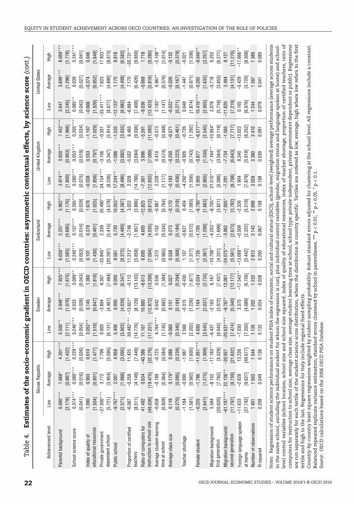
EQUITY IN STUDENT ACHIEVEMENT ACROSS OECD COUNTRIES: AN INVESTIGATION OF THE ROLE OF POLICIES
Table
4. E
stim
ates
of
the
soci
o-ec
onom
ic g
rad
ien
t in
OEC
D c
oun
trie
s: a
sym
met
ric
con
tex
tual
eff
ects
, by
scie
nce
sco
re (
cont
.)
Slov
ak R
epub
licSw
eden
Switz
erla
ndU
nite
d Ki
ngdo
mUn
ited
Stat
es
Achi
evem
ent l
evel
Low
Aver
age
High
Low
Aver
age
High
Low
Aver
age
High
Low
Aver
age
High
Low
Aver
age
High
Pare
ntal
bac
kgro
und
6.09
0***
1.66
8*4.
301*
**5.
506*
*3.
948*
**7.
925*
**6.
039*
**2.
207*
**5.
902*
**3.
974*
*3.
920*
**7.
452*
**3.
647
3.69
9***
8.06
9***
[2.1
78]
[0.8
87]
[1.4
32]
[2.1
11]
[1.0
76]
[1.6
75]
[1.5
83]
[0.6
95]
[1.1
76]
[1.9
00]
[0.9
53]
[1.9
66]
[2.2
45]
[1.2
96]
[1.7
78]
Scho
ol s
cien
ce s
core
0.37
4***
0.08
9***
0.22
9***
0.24
6***
0.03
30.
089*
*0.
240*
**0.
107*
**0.
265*
**0.
280*
**0.
053*
**0.
205*
**0.
085*
*0.
039
0.24
1***
[0.0
41]
[0.0
16]
[0.0
26]
[0.0
54]
[0.0
28]
[0.0
43]
[0.0
53]
[0.0
14]
[0.0
29]
[0.0
75]
[0.0
19]
[0.0
24]
[0.0
42]
[0.0
27]
[0.0
41]
Inde
x of
qua
lity
of
educ
atio
nal r
esou
rces
1.09
00.
903
0.61
03.
052*
*0.
145
1.36
00.
101
0.37
91.
678
–0.0
380.
553
–1.1
97–0
.666
–0.3
740.
046
[1.5
04]
[0.8
01]
[1.4
77]
[1.5
18]
[0.8
47]
[1.8
16]
[1.4
30]
[0.4
81]
[1.0
25]
[1.8
56]
[0.7
97]
[1.0
29]
[1.5
26]
[0.8
52]
[1.6
48]
Priv
ate
gove
rnm
ent
depe
nden
t sch
ool
–27.
500*
**3.
772
7.79
90.
000
–3.8
046.
307
–33.
845*
2.33
935
.490
***
34.1
54**
*–3
.156
–0.3
51–3
3.41
1***
7.62
317
.933
**[5
.721
][3
.954
][5
.595
][6
.131
][4
.467
][7
.484
][2
0.29
7][5
.415
][4
.578
][8
.336
][5
.347
][5
.914
][8
.077
][4
.890
][8
.673
]Pu
blic
sch
ool
–9.7
67**
*2.
007
4.95
85.
406
0.00
00.
000
9.56
15.
730
10.0
53**
17.2
44**
–1.0
86–1
.535
–12.
123*
1.17
08.
818
[2.5
71]
[1.9
88]
[3.0
95]
[5.6
03]
[4.0
39]
[6.5
47]
[9.3
72]
[4.4
89]
[4.3
87]
[8.4
96]
[3.8
82]
[3.9
35]
[6.9
82]
[4.4
08]
[6.5
83]
Prop
ortio
n of
cer
tifie
d te
ache
rs–6
.087
–0.2
5811
.425
39.4
82**
*–1
3.65
1*–0
.112
11.3
13*
–2.7
483.
022
2.02
8–5
.022
8.46
5–6
.884
7.17
0–2
0.73
1**
[8.5
11]
[4.1
49]
[7.4
49]
[14.
776]
[8.1
29]
[13.
103]
[5.8
58]
[1.9
57]
[3.8
86]
[14.
766]
[3.6
94]
[9.0
36]
[7.4
08]
[6.4
26]
[9.6
59]
Ratio
of c
ompu
ters
for
inst
ruct
ion
to s
choo
l size
41.4
920.
634
–40.
386
11.1
6710
.880
–6.6
136.
695
4.60
5–1
2.82
5–7
.361
3.88
6–5
.591
–9.0
36–0
.668
1.71
8[4
9.03
6][1
9.47
5][3
2.27
6][1
7.25
1][1
2.87
2][1
3.20
6][7
.004
][4
.035
][8
.612
][1
2.93
2][7
.089
][1
1.09
3][1
2.42
3][5
.816
][9
.280
]Av
erag
e st
uden
t lea
rnin
g tim
e at
sch
ool
–0.6
58–0
.189
–0.7
234.
764*
**0.
642
0.53
61.
272
0.15
2–0
.987
2.22
8**
0.41
0–0
.373
2.19
3*0.
967*
–2.1
08**
[0.8
28]
[0.3
64]
[0.5
84]
[1.7
45]
[0.8
82]
[1.3
84]
[0.9
65]
[0.3
34]
[0.7
64]
[1.1
17]
[0.5
74]
[0.9
48]
[1.1
47]
[0.5
76]
[1.0
14]
Aver
age
clas
s si
ze0.
119
0.17
9*0.
086
–0.0
600.
151
0.02
70.
558
0.27
3–0
.170
–0.1
83–0
.250
–0.5
71–0
.522
*–0
.026
–0.1
32[0
.270
][0
.095
][0
.239
][0
.346
][0
.184
][0
.294
][0
.368
][0
.184
][0
.318
][0
.436
][0
.223
][0
.461
][0
.271
][0
.167
][0
.379
]Te
ache
r sho
rtage
–1.1
84–0
.690
–1.9
872.
566
–0.3
15–0
.430
1.10
7–0
.627
0.40
4–4
.292
***
–0.9
26–0
.726
0.64
8–1
.447
–0.0
21[1
.581
][0
.562
][1
.605
][2
.202
][1
.226
][1
.877
][1
.377
][0
.572
][1
.093
][1
.556
][0
.743
][1
.292
][1
.874
][0
.871
][1
.336
]Fe
mal
e st
uden
t–0
.225
–1.7
86–1
1.95
1***
4.93
01.
164
–2.0
34–1
.735
–1.7
05–6
.790
***
2.95
5–0
.877
–6.5
77**
10.4
16**
*–0
.282
–8.0
40**
[2.6
41]
[1.2
75]
[1.9
09]
[3.5
45]
[2.0
37]
[2.7
33]
[2.3
67]
[1.2
99]
[1.8
83]
[2.8
65]
[1.3
30]
[2.5
45]
[2.9
55]
[1.6
32]
[3.2
57]
Mig
ratio
n ba
ckgr
ound
:fir
st g
ener
atio
n5.
584
–8.1
52–1
7.18
3***
–6.4
37–2
.163
6.16
7–1
0.70
8**
–4.2
53**
–8.7
05**
21.5
10**
*–7
.164
**–1
0.95
4*2.
078
–0.7
186.
252
[20.
620]
[7.7
62]
[5.5
29]
[8.0
43]
[3.9
72]
[7.4
37]
[4.3
31]
[1.6
99]
[3.8
21]
[5.0
86]
[3.5
64]
[6.1
19]
[5.7
18]
[3.6
53]
[6.2
71]
Mig
ratio
n ba
ckgr
ound
: se
cond
gen
erat
ion
–61.
197*
**22
.126
**–2
0.92
7–2
0.63
1***
–9.7
87*
13.0
61–2
4.07
5***
–3.9
62–7
.005
*–7
.291
–7.7
34–1
.565
–11.
620
2.48
48.
127
[11.
797]
[8.7
39]
[21.
632]
[7.4
74]
[5.3
40]
[12.
177]
[5.5
61]
[2.6
73]
[3.7
82]
[8.7
98]
[6.6
43]
[7.7
17]
[7.2
19]
[4.1
31]
[11.
276]
Fore
ign
lang
uage
spo
ken
at h
ome
–11.
633
–2.6
2813
.226
–7.0
303.
375
–17.
542*
*–1
3.08
9**
–0.5
09–2
.326
1.90
48.
340
–13.
022
0.16
5–5
.429
–17.
666*
*[2
7.74
2][9
.627
][4
9.67
7][7
.350
][4
.089
][6
.726
][5
.442
][2
.322
][5
.519
][7
.879
][5
.918
][8
.252
][6
.976
][3
.720
][8
.508
]Nu
mbe
r of o
bser
vatio
ns1
401
150
31
544
113
51
202
123
22
912
314
22
899
302
83
380
341
01
244
139
71
389
R-sq
uare
d0.
208
0.04
90.
138
0.13
20.
034
0.03
80.
200
0.06
70.
158
0.10
80.
039
0.09
10.
079
0.04
10.
089
Not
es:
Reg
ress
ion
of
stu
den
t sc
ien
ce p
erfo
rman
ce o
n s
tud
ent
PISA
ind
ex o
f eco
nom
ic, s
ocia
l an
d c
ult
ura
l sta
tus
(ES
CS)
, sch
ool-
leve
l (w
eigh
ted
) ave
rage
per
form
ance
(ave
rage
acr
oss
stu
den
tsin
th
e sa
me
sch
ool
, exc
lud
ing
the
ind
ivid
ual
stu
den
t fo
r w
ho
m t
he
regr
essi
on is
ru
n),
plu
s in
div
idu
al c
ontr
ol v
aria
bles
(gen
der
, mig
rati
on
sta
tus
and
lan
guag
e sp
oken
at
hom
e) a
nd
sch
ool-
leve
l co
ntr
ol v
aria
bles
(sc
hoo
l lo
cati
on,
sch
ool
size
an
d s
choo
l si
ze s
qu
ared
, in
dex
of
qu
alit
y of
ed
uca
tion
al r
esou
rces
, in
dex
of
teac
her
sh
ort
age,
pro
por
tio
n o
f ce
rtif
ied
tea
cher
s, r
atio
of
com
pu
ters
for
inst
ruct
ion
to
sch
ool s
ize,
ave
rage
cla
ss s
ize,
ave
rage
stu
den
t le
arn
ing
tim
e at
sch
ool,
sch
ool t
ype:
pri
vate
ind
epen
den
t, p
riva
te g
over
nm
ent
dep
end
ent
or
pu
blic
). R
egre
ssio
ns
are
run
sep
arat
ely
for
each
ter
tile
of
the
stu
den
t sc
ien
ce s
core
dis
trib
uti
on, w
her
e th
e d
istr
ibu
tion
is c
ou
ntr
y sp
ecif
ic. T
erti
les
are
ord
ered
as
low
, ave
rage
, hig
h w
her
e lo
w r
efer
s to
th
e fi
rst
tert
ile
and
hig
h t
o th
e la
st. R
egre
ssio
ns
for
Ital
y in
clu
de
regi
on
al f
ixed
eff
ects
.C
oun
try-
by-c
oun
try
leas
t-sq
uar
e re
gres
sion
s w
eigh
ted
by
stu
den
t sa
mp
lin
g p
roba
bili
ty. R
obu
st s
tan
dar
d e
rro
rs a
dju
sted
fo
r cl
ust
erin
g at
th
e sc
hoo
l lev
el. A
ll r
egre
ssio
ns
incl
ud
e a
con
stan
t.B
alan
ced
rep
eate
d r
epli
cate
var
ian
ce e
stim
atio
n, s
tan
dar
d e
rro
rs c
lust
ered
by
sch
ool
in p
aren
thes
es, *
** p
<0.
01, *
* p
<0.
05, *
p<
0.1.
Sou
rce:
OEC
D c
alcu
lati
ons
base
d o
n t
he
2006
OEC
D P
ISA
Dat
abas
e.
OECD JOURNAL: ECONOMIC STUDIES – VOLUME 2010/1 © OECD 201022

EQUITY IN STUDENT ACHIEVEMENT ACROSS OECD COUNTRIES: AN INVESTIGATION OF THE ROLE OF POLICIES
Social gains from reallocating students across schools and/or classes are realised if
there is no adverse effect of social heterogeneity per se on educational achievement.
Students may be influenced, not only by the mean level of peer quality, but also by the
diversity of their peers. Regression results presented in Table 5 suggest that in most OECD
countries there is no adverse effect of social heterogeneity on student performance. The
effect of social heterogeneity on educational achievement is tested by including the
standard deviation of the student socio-economic background in each school. The
regressions also control for student and school-level characteristics (socio-economic
intake, location, resources, size, ownership and funding). The impact of social
heterogeneity is statistically insignificant for 26 out of 29 countries, the exceptions being
Italy, the Czech Republic, and Finland, where a negative impact is found. These results are
only suggestive, given that, due to data limitations, the data used is school-level as
opposed to class-level, which would be needed to properly analyse peer effects. Taken at
face value, the results reported in Tables 4 and 5 suggest that in some countries increasing
school mix could achieve equity and efficiency goals, particularly in highly socially-
segregated countries.
3. The impact of policies on equity in education achievement acrossOECD countries
3.1. Motivation
As one of the major mechanisms through which economic advantages and
disadvantages are transmitted, education plays a central role in intergenerational social
mobility. This makes it, by the same token, an accessible policy instrument to increase
intergenerational social mobility. Indeed, while there is little scope nor rationale for
attenuating inequalities arising from the transmission of inheritable factors, inequalities
in the distribution of learning opportunities might signal economic inefficiencies
potentially amenable to policy intervention. Cross-country empirical analysis allows
examining to what extent different institutions would moderate or reinforce the
relationship between socio-economic background and student performance.
Research in this field has generally focused on the role of educational policies and
institutions. Institutional features such as early intervention, education, welfare and
redistribution policies are likely to have an impact on equity in student achievement in
OECD countries. This section describes the empirical approach undertaken in trying to
identify the effects of policies at the cross-country level, and presents and discusses the
relevant results, in the light of those already provided in the literature.
3.2. Empirical approach
3.2.1. The model
The baseline empirical approach for analysing the impact of policies on equity in
educational achievement in this study is based on two cross-country variants of equation (2):
(4a)
(4b)
where Xisc denotes student characteristics, Zsc denotes school characteristics, Wc denotes
country-level variables, and Cc denotes country fixed effects. In these equations, all school
and student-level characteristics display country-specific coefficients. Equations (4a) and
(4b) describe country-specific models, in which only the impact of the variables Fisc,
isccsccisccscbiscwisc WZXFFY 1
isccsccisccscbiscwisc CZXFFY 1
scF
OECD JOURNAL: ECONOMIC STUDIES – VOLUME 2010/1 © OECD 2010 23

EQUITY IN STUDENT ACHIEVEMENT ACROSS OECD COUNTRIES: AN INVESTIGATION OF THE ROLE OF POLICIES
Table
5. E
stim
ates
of
the
soci
o-ec
onom
ic g
rad
ien
t in
OEC
D c
oun
trie
s: t
he
imp
act
of h
eter
ogen
eity
in
th
e sc
hoo
l en
viro
nm
ent
Aust
riaBe
lgiu
mCa
nada
Czec
h Re
publ
icFi
nlan
dGe
rman
yG
reec
eHu
ngar
yIc
elan
dIre
land
Italy
Japa
nKo
rea
Indi
vidu
al b
ackg
roun
d7.
696*
**17
.404
***
25.5
81**
*22
.923
***
28.5
20**
*15
.333
***
18.1
39**
*8.
202*
**27
.739
***
30.2
26**
*9.
354*
**7.
097*
**10
.383
***
[1.8
84]
[1.0
80]
[1.7
40]
[1.6
20]
[1.6
84]
[1.3
71]
[1.6
46]
[1.5
89]
[1.9
89]
[1.8
54]
[1.3
27]
[1.9
83]
[1.7
74]
Scho
ol e
nviro
nmen
t68
.751
***
58.5
53**
*29
.425
***
75.6
75**
*4.
067
70.9
16**
*31
.300
***
73.0
48**
*12
.700
*37
.553
***
79.5
72**
*98
.088
***
59.5
08**
*
[8.4
65]
[7.0
40]
[5.9
88]
[9.2
00]
[6.7
83]
[7.9
29]
[7.1
20]
[5.0
02]
[6.5
09]
[6.5
32]
[4.7
51]
[11.
711]
[9.4
40]
Scho
ol-le
vel E
SCS
stan
dard
dev
iatio
n11
.512
30.5
20–1
3.23
9–7
0.33
5**
–44.
579*
*–5
.041
8.99
614
.363
–5.5
126.
143
–94.
208*
**–3
9.73
66.
505
[26.
674]
[19.
396]
[18.
871]
[29.
087]
[18.
374]
[16.
025]
[22.
138]
[15.
348]
[17.
724]
[21.
362]
[19.
720]
[34.
285]
[30.
606]
Inde
x of
qua
lity
of e
duca
tiona
l res
ourc
es1.
555
1.50
1–0
.095
–2.2
07–3
.150
2.92
20.
361
–0.5
22–1
.776
4.13
75.
229*
*1.
120
4.06
1
[3.4
12]
[3.2
64]
[2.0
88]
[4.0
59]
[2.4
13]
[2.7
42]
[3.7
81]
[2.5
64]
[2.0
35]
[3.0
51]
[2.3
99]
[2.7
60]
[3.3
79]
Priv
ate
gove
rnm
ent d
epen
dent
sch
ool
–78.
602*
**–5
.493
6.01
796
.429
**0.
715
45.0
64**
0.00
016
.142
123.
954*
**30
.314
***
50.5
75**
–70.
706*
**0.
760
[21.
680]
[9.5
07]
[11.
610]
[46.
218]
[10.
901]
[20.
661]
[0.0
00]
[17.
194]
[39.
970]
[8.8
82]
[19.
639]
[8.5
31]
[8.2
41]
Publ
ic s
choo
l–7
8.95
4***
–17.
113*
–12.
864
126.
164*
**0.
000
40.7
45**
*27
.990
**16
.100
167.
977*
**18
.520
*46
.852
***
51.2
66**
*5.
199
[22.
173]
[9.1
68]
[9.1
35]
[47.
755]
[6.9
31]
[14.
130]
[11.
433]
[16.
419]
[33.
815]
[9.4
72]
[12.
265]
[6.6
49]
[6.7
11]
Prop
ortio
n of
cer
tifie
d te
ache
rs–0
.956
12.9
71–5
.842
–1.9
802.
292
3.74
7–2
1.97
538
.816
**47
.234
**26
.410
*11
.876
–46.
650*
**–3
4.35
8***
[16.
197]
[11.
912]
[8.9
17]
[20.
162]
[7.8
69]
[13.
100]
[25.
667]
[16.
148]
[22.
472]
[14.
293]
[12.
802]
[16.
177]
[10.
034]
Ratio
of c
ompu
ters
for i
nstru
ctio
n to
sch
ool s
ize27
.469
42.3
75**
20.0
8771
.926
*12
.004
–13.
518
47.7
8041
.407
**–1
3.01
229
.473
22.2
3621
.478
17.0
23
[19.
052]
[18.
628]
[13.
261]
[42.
964]
[20.
975]
[55.
118]
[36.
276]
[19.
693]
[27.
670]
[51.
566]
[21.
593]
[17.
190]
[24.
061]
Aver
age
stud
ent l
earn
ing
time
at s
choo
l6.
960*
**7.
181*
**1.
782*
5.38
0***
4.75
7***
7.22
9***
16.6
65**
*10
.367
***
4.55
6***
4.43
4**
7.56
3***
8.64
5***
11.8
89**
*
[2.1
29]
[1.1
43]
[0.9
49]
[1.4
78]
[1.4
93]
[1.4
43]
[1.7
44]
[1.4
85]
[1.4
81]
[1.7
63]
[1.0
91]
[1.7
75]
[1.4
48]
Aver
age
clas
s si
ze2.
256*
**0.
870
1.47
7***
1.79
1***
0.20
31.
701*
*0.
570*
*0.
625*
–0.3
59*
0.85
8–0
.707
**1.
329*
**–1
.155
[0.6
36]
[0.5
66]
[0.3
80]
[0.6
01]
[0.2
77]
[0.7
83]
[0.2
41]
[0.3
33]
[0.2
06]
[0.6
65]
[0.2
98]
[0.4
49]
[1.0
12]
Teac
her s
horta
ge–2
.281
–10.
630*
**1.
215
–12.
070*
*–4
.233
–3.7
330.
123
–0.3
36–4
.319
**2.
381
9.03
9***
1.28
00.
446
[4.6
09]
[2.2
83]
[1.6
64]
[5.3
24]
[2.9
63]
[3.1
94]
[3.0
04]
[4.2
64]
[1.6
85]
[2.5
51]
[2.7
61]
[5.1
83]
[2.9
44]
Fem
ale
stud
ent
–11.
769*
**–9
.326
***
–7.0
09**
*–9
.874
**1.
268
–11.
796*
**–3
.965
–23.
765*
**5.
321*
–0.1
88–1
0.30
3***
–3.5
770.
828
[3.9
97]
[3.0
64]
[2.3
05]
[3.8
70]
[3.0
03]
[2.7
22]
[3.0
66]
[2.5
79]
[3.1
39]
[3.7
03]
[2.8
44]
[3.2
04]
[3.4
56]
Mig
ratio
n ba
ckgr
ound
: firs
t gen
erat
ion
–35.
519*
**–9
.686
**–6
.086
–49.
082*
**–5
8.70
6**
–32.
195*
**–2
3.00
3–4
3.11
2***
–21.
747
–22.
897
–47.
386*
*–1
6.84
614
.649
*
[8.4
74]
[4.7
88]
[4.6
29]
[14.
601]
[27.
260]
[6.9
27]
[15.
703]
[15.
813]
[20.
300]
[14.
903]
[21.
192]
[43.
729]
[7.8
71]
Mig
ratio
n ba
ckgr
ound
: sec
ond
gene
ratio
n–3
6.63
6***
–31.
825*
**–1
2.12
4–3
4.45
0***
–79.
701*
**–1
9.48
1***
1.78
24.
967
–30.
929
14.3
58–3
8.39
5***
34.4
620.
000
[6.8
97]
[9.8
08]
[7.3
57]
[12.
642]
[16.
283]
[6.6
35]
[10.
613]
[8.0
13]
[20.
233]
[9.0
48]
[8.8
97]
[28.
111]
[0.0
00]
Fore
ign
lang
uage
spo
ken
at h
ome
–30.
334*
**–2
5.59
6***
–3.4
11–1
.757
–6.0
08–2
6.41
7***
–28.
464*
**–1
8.84
5–3
5.99
2**
–84.
296*
**–5
.474
–104
.619
***
5.04
5
[8.3
43]
[6.0
40]
[7.3
56]
[13.
795]
[12.
892]
[6.1
44]
[8.9
09]
[12.
120]
[15.
737]
[13.
616]
[11.
163]
[21.
964]
[29.
504]
Num
ber o
f obs
erva
tions
418
26
246
1453
85
112
428
43
270
346
74
014
329
43
492
1442
05
485
492
1
R-sq
uare
d0.
432
0.44
80.
109
0.37
70.
106
0.47
90.
389
0.49
60.
094
0.18
40.
334
0.35
10.
255
OECD JOURNAL: ECONOMIC STUDIES – VOLUME 2010/1 © OECD 201024

EQUITY IN STUDENT ACHIEVEMENT ACROSS OECD COUNTRIES: AN INVESTIGATION OF THE ROLE OF POLICIES
Table
5.Es
tim
ates
of
the
soci
o-ec
onom
ic g
rad
ien
t in
OEC
D c
oun
trie
s: t
he
imp
act
of h
eter
ogen
eity
in
th
e sc
hoo
l en
viro
nm
ent
(con
t.)
Luxe
mbo
urg
Mex
ico
Neth
erla
nds
New
Zea
land
Norw
ayPo
land
Portu
gal
Slov
ak
Repu
blic
Swed
enSw
itzer
land
Unite
d Ki
ngdo
mUn
ited
Stat
es
Indi
vidu
al b
ackg
roun
d16
.690
***
7.71
4***
9.97
9***
39.9
34**
*29
.216
***
36.2
34**
*18
.034
***
20.5
20**
*30
.535
***
20.6
41**
*34
.881
***
31.7
95**
*[1
.502
][0
.869
][1
.105
][2
.146
][1
.977
][1
.509
][1
.281
][1
.526
][2
.294
][1
.628
][2
.274
][1
.967
]Sc
hool
env
ironm
ent
48.8
95**
*24
.484
***
87.6
07**
*33
.240
***
28.9
55**
13.5
18*
18.9
83**
*55
.758
***
22.4
54**
*52
.701
***
50.1
86**
*22
.614
***
[5.4
38]
[3.7
32]
[7.3
52]
[8.5
18]
[11.
056]
[7.9
72]
[4.2
97]
[9.3
04]
[7.5
37]
[5.4
29]
[7.5
20]
[7.0
98]
Scho
ol-le
vel E
SCS
stan
dard
dev
iatio
n–1
0.82
3–1
7.45
980
.293
***
–5.5
572.
026
16.9
7815
.020
–18.
543
4.32
24.
948
0.72
842
.986
*[1
3.60
9][1
1.29
0][2
3.79
4][1
4.81
5][1
5.81
9][1
9.48
6][1
3.65
1][2
3.83
8][1
6.54
4][1
4.55
4][1
6.24
0][2
4.95
7]In
dex
of q
ualit
y of
edu
catio
nal r
esou
rces
5.25
0***
3.41
9*8.
154*
**–3
.495
–5.6
95–1
.447
–0.9
74–3
.042
3.89
14.
325*
*–0
.679
1.92
1[1
.503
][2
.051
][2
.918
][2
.519
][4
.115
][2
.172
][2
.733
][3
.959
][2
.446
][1
.936
][2
.582
][2
.864
]Pr
ivat
e go
vern
men
t dep
ende
nt s
choo
l4.
233
0.00
05.
693
0.00
00.
000
–17.
653
12.3
8710
.220
22.6
38–1
2.96
40.
882
–12.
359
[5.3
79]
[0.0
00]
[7.3
64]
[0.0
00]
[40.
915]
[23.
190]
[20.
492]
[14.
451]
[22.
399]
[54.
348]
[19.
352]
[15.
293]
Publ
ic s
choo
l0.
000
18.7
020.
000
–9.5
79–4
0.36
8–2
2.56
74.
788
19.2
39**
*0.
000
45.3
30**
*–0
.753
–6.9
68[4
.483
][1
1.76
1][5
.046
][9
.238
][3
7.83
4][2
1.40
0][2
1.36
5][6
.950
][2
2.69
7][1
3.38
1][1
2.92
2][1
1.41
6]Pr
opor
tion
of c
ertif
ied
teac
hers
35.8
42**
*–1
1.28
5*–4
.277
–4.5
96–2
2.40
3***
25.9
413.
826
14.4
3775
.488
***
–8.3
605.
820
–5.6
56[1
2.04
5][6
.200
][1
3.97
0][6
.577
][7
.426
][2
0.39
8][1
3.52
8][1
6.85
6][2
6.14
9][6
.962
][1
8.11
6][2
3.67
9]Ra
tio o
f com
pute
rs fo
r ins
truct
ion
to s
choo
l size
3.91
540
.392
–180
.837
***
17.2
5018
.044
0.14
511
9.19
427
2.31
6***
25.7
7919
.889
–14.
671
–17.
979
[9.6
91]
[36.
156]
[39.
716]
[23.
920]
[39.
939]
[37.
200]
[72.
419]
[80.
312]
[30.
638]
[16.
739]
[23.
610]
[18.
318]
Aver
age
stud
ent l
earn
ing
time
at s
choo
l10
.420
***
5.86
4***
6.98
5***
10.6
45**
*5.
353*
**5.
310*
*12
.504
***
3.62
9***
7.81
9***
8.33
6***
7.37
4***
9.49
4***
[1.8
85]
[1.1
45]
[1.7
11]
[2.0
48]
[1.7
79]
[2.2
15]
[1.5
71]
[1.3
01]
[2.6
28]
[1.5
18]
[2.2
56]
[2.0
05]
Aver
age
clas
s si
ze–0
.172
0.40
2**
0.99
60.
592
–0.1
770.
721
0.65
10.
823
0.30
11.
515*
*–0
.541
0.19
1[0
.568
][0
.166
][0
.607
][0
.692
][0
.265
][0
.712
][0
.505
][0
.654
][0
.537
][0
.613
][0
.764
][0
.825
]Te
ache
r sho
rtage
12.2
53**
*0.
698
1.12
2–5
.533
**1.
303
0.47
0–6
.897
–11.
738*
**3.
079
–1.5
21–3
.880
*1.
186
[2.5
46]
[2.0
13]
[3.1
46]
[2.5
30]
[3.5
67]
[4.8
60]
[4.2
77]
[3.6
41]
[3.0
67]
[2.2
76]
[2.3
13]
[2.8
36]
Fem
ale
stud
ent
–7.0
69**
–8.6
43**
*–1
2.52
0***
–6.7
96*
3.85
6–1
.673
–2.1
93–1
0.20
7***
–0.3
60–1
3.93
0***
–10.
512*
**–5
.117
*[2
.707
][2
.745
][2
.424
][3
.921
][3
.787
][2
.339
][2
.385
][3
.191
][2
.848
][2
.316
][2
.888
][2
.597
]M
igra
tion
back
grou
nd: f
irst g
ener
atio
n–2
2.71
6***
–37.
027*
**–3
0.34
2***
–5.8
29–3
7.07
9***
40.8
18–3
2.55
4***
–22.
822
–9.6
83–3
4.73
8***
–4.3
16–3
.265
[4.4
31]
[10.
721]
[5.8
48]
[5.9
86]
[10.
793]
[57.
433]
[9.2
25]
[18.
419]
[8.4
31]
[4.0
48]
[6.8
85]
[7.4
13]
Mig
ratio
n ba
ckgr
ound
: sec
ond
gene
ratio
n–2
2.39
2***
–65.
729*
**–2
7.32
6***
–7.5
46–1
7.75
3–8
6.46
1**
–49.
162*
**–4
4.72
4–2
7.64
1**
–55.
692*
**–1
2.98
6–8
.402
[5.1
35]
[11.
224]
[9.4
90]
[6.4
24]
[14.
385]
[42.
389]
[9.6
23]
[30.
291]
[10.
776]
[5.8
09]
[10.
839]
[9.8
15]
Fore
ign
lang
uage
spo
ken
at h
ome
–22.
493*
**44
.471
–13.
254*
–28.
072*
**–9
.937
1.88
88.
012
–13.
251
–27.
341*
**–2
4.21
2***
–9.8
08–1
5.40
4**
[4.3
58]
[27.
115]
[7.3
33]
[6.9
40]
[10.
769]
[15.
796]
[8.7
50]
[22.
660]
[8.4
32]
[4.5
28]
[11.
191]
[6.7
97]
Num
ber o
f obs
erva
tions
395
713
041
401
23
659
386
85
126
418
24
448
356
98
953
981
84
030
R-sq
uare
d0.
369
0.31
90.
535
0.23
20.
099
0.16
40.
307
0.30
60.
150
0.36
20.
204
0.20
9
Not
es:
Reg
ress
ion
of
stu
den
t sc
ien
ce p
erfo
rman
ce o
n s
tud
ent
PISA
in
dex
of
econ
omic
, soc
ial
and
cu
ltu
ral
stat
us
(ESC
S), i
nd
ivid
ual
con
trol
var
iabl
es (
mig
rati
on
sta
tus
and
lan
guag
e sp
oke
nat
hom
e), s
cho
ol-l
evel
ESC
S (a
vera
ge a
cro
ss s
tud
ents
in t
he
sam
e sc
hoo
l, ex
clu
din
g th
e in
div
idu
al s
tud
ent
for
wh
om t
he
regr
essi
on
is r
un
), sc
hoo
l–le
vel s
tan
dar
d d
evia
tion
in s
tud
ent
soci
o-ec
on
om
ic b
ackg
rou
nd
(ca
lcu
late
d u
sin
g st
ud
ent-
leve
l w
eigh
ts),
and
sch
ool-
leve
l co
ntr
ols
(sc
hoo
l lo
cati
on,
sch
ool
size
an
d s
choo
l si
ze s
qu
ared
, in
dex
of
qu
alit
y o
f ed
uca
tion
al r
eso
urc
es,
ind
ex o
f te
ach
er s
hor
tage
, pro
por
tion
of
cert
ifie
d t
each
ers,
rat
io o
f co
mp
ute
rs f
or
inst
ruct
ion
to
sch
oo
l siz
e, a
vera
ge c
lass
siz
e, a
vera
ge s
tud
ent
lear
nin
g ti
me
at s
cho
ol, s
cho
ol t
ype:
pri
vate
ind
epen
den
t, p
riva
te g
over
nm
ent
dep
end
ent,
pu
blic
), re
gres
sio
ns
for
Ital
y in
clu
de
regi
on
al f
ixed
eff
ects
(n
ot
rep
ort
ed).
Co
un
try-
by-c
oun
try
leas
t-sq
uar
e re
gres
sion
s w
eigh
ted
by
stu
den
tsa
mp
lin
g p
rob
abil
ity.
Ro
bust
sta
nd
ard
err
ors
adju
sted
fo
r cl
ust
erin
g at
th
e sc
ho
ol l
evel
. Reg
ress
ion
s fo
r It
aly
incl
ud
e re
gio
nal
fix
ed e
ffec
ts.
Bal
ance
d r
epea
ted
rep
lica
te v
aria
nce
est
imat
ion
, sta
nd
ard
err
ors
clu
ster
ed b
y sc
ho
ol in
par
enth
eses
, ***
p<
0.01
, **
p<
0.05
, * p
<0.
1. A
ll r
egre
ssio
ns
incl
ud
e a
con
stan
t.So
urc
e:O
ECD
cal
cula
tion
s ba
sed
on
th
e20
06 O
ECD
PIS
A D
atab
ase.
OECD JOURNAL: ECONOMIC STUDIES – VOLUME 2010/1 © OECD 2010 25

EQUITY IN STUDENT ACHIEVEMENT ACROSS OECD COUNTRIES: AN INVESTIGATION OF THE ROLE OF POLICIES
and country-level variables is restricted to be equal across countries. The difference
between equations (4a) and (4b) is that equation (4b) allows country-specific intercepts
whereas equation (4a) allows estimating the direct impact of country-specific variables.
Because of the presence of country fixed effects, equation (4b) is to be considered as less
restrictive in terms of cross-country homogeneity assumptions.
The choice of the control variables included in models (4a) and (4b) is based on
the “education production function” approach (see e.g. Hanushek, 1994). The variables
included are: individual characteristics (gender, migration status and language spoken at
home), school location (small town or village, city), school size and school size squared,
school resources (index of quality of educational resources, index of teacher shortage,
proportion of certified teachers, ratio of computers for instruction to school size), average
class size, average student learning time at school, and school type (private independent,
private government dependent, public). These variables are allowed to have a
heterogeneous impact across countries. Therefore, the findings on the impact of country-
level features on equity in student achievement do not depend on the country-level effect
of student and schools characteristics on student performance.23 Baseline estimates of
equation (4a) also include GDP per capita as a control variable, as usually done in
comparable empirical studies.
3.2.2. How policies and institutions are modelled
Policies and institutions are introduced in the model by assuming that the influence of
student and school socio-economic background varies across institutional regimes. In this
specification, it is no longer required that parameters w and b and are equal across
countries. These parameters are made regime-specific, by introducing policy interaction
terms:
(5a)
(5b)
where Pc denotes policies or system-level features. Specifications (5a) and (5b) identify
whether institutional features affect the impact of student and school background on
achievement. In specification (5b), which includes country fixed effects, it is not possible to
estimate the direct effect of institutional features on student performance, given that
those do not vary within countries.
Variants of models (5a) and (5b) are estimated, depending on the nature of the policy
under consideration. While both policy interaction terms may be relevant for education
policies, it can be argued that welfare, redistributive and labour market policies are
generally targeted towards households or individuals and should, therefore, have no direct
impact on school environment effects. Thus, for these policies, only the interactions with
the individual background, within-school effect are considered. In this case, the model is
further relaxed by assuming that the impact of schools’ socio-economic background is
country-specific. In terms of the above equations, only parameter w does not vary across
countries (but varies across institutional regimes).24
As already mentioned, specification (5b) is more restrictive in terms of model
assumptions than specification (5a) but it provides estimates of the direct impact of
policies on student achievement. Hence, in theory it might allow investigating whether
iscccscc
isccsccbisccwscbiscwisc
WPZ
XFPFPFFY
1
isccscc
isccsccbisccwscbiscwisc
CZ
XFPFPFFY
1
OECD JOURNAL: ECONOMIC STUDIES – VOLUME 2010/1 © OECD 201026

EQUITY IN STUDENT ACHIEVEMENT ACROSS OECD COUNTRIES: AN INVESTIGATION OF THE ROLE OF POLICIES
there is a trade-off between efficiency – increasing students’ overall performance – and
equity – reducing the dependence of performance on socio-economic background.
However, caution is needed in this respect. Due to the very limited degrees of freedom
under which the corresponding parameter is estimated, the specification cannot provide a
consistent estimate of the causal impact of system-level features on student performance.
As will appear clear below, given the very unrestricted nature of the model in terms of
country heterogeneity, the direct impact of policies on performance is weakly identified.
Moreover, the main purpose of this analysis is to assess the influence of policies on equity
in education, rather than gauging the average impact of institutions on student and school
performance, which is extensively discussed in PISA reports (see, for instance, OECD,
2007a). Hence, discussion of regression results will focus on interaction effects, rather than
the direct impact of policies.
The institutional features are all measured at the country level. While most of them
are systemic by definition and, therefore, do not vary within countries, others have a
within-country dimension, such as school level policy settings – class sizes, proportion of
qualified teachers, school selectivity, or ability grouping.25 These variables are, however,
averaged at the country level (using school weights), and the analysis only uses between-
country variation in policies and institutions. Indeed, the extent of within-country
variation in school-level features is very low and selection bias, whereby students with the
same parental background would be found in schools applying certain policies,26 would
make the identification of causal effects difficult. For example, rich families are likely to
opt to send their children to schools with high resource levels or highly-qualified teachers.
Also, in systems where countries provide disadvantaged areas with additional resources, it
is possible to observe an opposite selection bias, whereby disadvantaged students
self-select into targeted schools that display specific features – such as lower class sizes.
Relying only on between-country variation in policies also makes it easier to interpret
results from a policy perspective.27 However, one drawback of this approach is that the
degrees of freedom at the country level are limited, which prevents from investigating
potential interactions among policies themselves, and in their relationship with equity in
student performance. It is also impossible to introduce various policies simultaneously in
the equation, with the associated risk that one policy-specific effect might capture the
effect of another, omitted and correlated policy.28
The cross-country regressions include a maximum of 27 OECD countries. Due to the
heterogeneity of Turkey and Mexico in terms of overall socio-economic background, these
OECD countries are excluded from the sample. Indeed, the average ESCS level for students
in these countries is a full standard deviation below the international mean, suggesting
that the comparisons between these countries and the rest of the OECD countries in terms
of equity in educational achievement may be misleading. Also, France is excluded from the
regressions since school principals did not respond to the PISA school questionnaire.29
3.2.2.1. Interpretation of the interaction effects. As already mentioned, specifications
(5a) and (5b) make it is possible to measure how within- and between-school socio-
economic effects vary across institutional regimes. Indeed, the impact of school and family
background varies across systems as follows:
and (6)cwwisc
isc PFY
cbbsc
isc PF
Y
OECD JOURNAL: ECONOMIC STUDIES – VOLUME 2010/1 © OECD 2010 27

EQUITY IN STUDENT ACHIEVEMENT ACROSS OECD COUNTRIES: AN INVESTIGATION OF THE ROLE OF POLICIES
A positive means that equity in education achievement decreases ( + > ) while a
negative means that it increases ( + < ) with the relevant policy.
Alternatively, specification (5a) also allows calculating the influence of policies at
different levels of the school and/or students’ socio-economic background, as follows:
(7)
In order to ease the interpretation, the policy variables are mean-centred so that
coefficient is to be interpreted as the impact of policy P at the cross-country average of
the schools’ and students’ socio-economic background distribution.30
Difficulties in identifying proper causal relationships between policies and equity in
educational achievement are enormous with the data at hand. As already mentioned, it is
not possible to disentangle nature from nurture effects in the (overall or within-school)
gradient estimation, nor is it possible to disentangle contextual from endogenous effects in
the between-school gradient estimation. Indeed, estimated within- and between-school
gradients are descriptive of the distribution in school performance, and should not be
interpreted in a causal sense. Yet, cross-country differences in the distribution of within-
and between-school gradients are likely to reflect to a large extent differences in policies
and institutions. Therefore, cross-country regression results concerning the role of policies
should not be influenced by the empirical limitations attached to the interpretation of the
estimated gradients. However, in order to properly identify the causal impact of policies,
one would need to be in a natural experiment setting, arising when specific reforms are put
in place within countries, and implemented differentially across “treated” and “control”
groups (such as the Pekkarinen et al., 2006 study on Finnish education reform in the 1970s).
Nonetheless, the cross-country analysis can still identify a number of policies and
institutions that are associated with higher levels of equity in educational achievement,
and, as such, potentially playing some role in influencing intergenerational social mobility.
3.3. Results on policies and equity in education achievement31
3.3.1. Education policies
Results of cross-country regressions in this section confirm that increasing education
spending has an ambiguous link with equity in educational opportunities, but other
aspects of the education system, such as differentiation policies and financial incentives
embedded in teachers’ remuneration, have a significant association with equality of
learning opportunities.
3.3.1.1. Education policies and school practices. One robust and common finding is that
early differentiation of students’ curricula tends to be associated with larger socio-economic
inequalities, with no corresponding gains in average performance. Both cross-country and
country-specific studies have highlighted the negative impact of ability tracking on
educational socio-economic inequalities (for cross-country evidence, see OECD, 2004, 2007a,
Schutz et al, 2005, Hanushek and Woessmann, 2005, Sutherland and Price, 2007, Duru-Bellat
and Suchaut, 2005, Amermuller, 2005; for country-specific evidence, see e.g. Bauer and
Riphahn, 2006, Pekkarinen et al., 2006, Holmlund, 2006, and Bratberg et al., 2005).32
Regression results confirm earlier findings according to which educational early
tracking increases socio-economic segregation between schools. Interpreting results
causally, when educational tracking is brought forward by one year, the impact of a school’s
scbiscwc
isc FFP
Y
OECD JOURNAL: ECONOMIC STUDIES – VOLUME 2010/1 © OECD 201028

EQUITY IN STUDENT ACHIEVEMENT ACROSS OECD COUNTRIES: AN INVESTIGATION OF THE ROLE OF POLICIES
environment on student performance would increase by 8.2 PISA science-score points.
Bringing forward tracking is associated with a much lower decrease in the within-school
relationship between students’ socio-economic background and science performance, by
2.9 PISA science-score points. Implied changes in the school environment effect are
quantitatively high, as they would range between 27.7 (PISA score points) in systems with
no tracking before age 16 to 77.1 (PISA score points) in systems with early tracking.33, 34 A
similar negative link with equity in educational achievement is found for the number of
school types programmes available to 15-year olds. This system-level variable indeed
captures the existence of early differentiation and, in this setting, polarisation of the
schooling system along socio-economic lines. Comparable results emerge also for selection
policy and ability grouping within schools.
Enrolment in vocational education is also associated with a higher impact of schools’
socio-economic background on student performance and a lower impact of an individual’s
background on student performance (Table 6a). Because disadvantaged students are
overrepresented in vocational training, it is found to exacerbate school socio-economic
inequalities, without increasing overall performance. This result is consistent
with empirical evidence on the German case. Buchel (2002) shows that lower-educated
school leavers are selected into apprenticeships with less favourable employment
prospects and, over time, they also find it increasingly difficult to transfer successfully
from apprenticeship to work.
However, the long-term effects of apprenticeship on individuals’ economic outcomes
are controversial.35 Moreover, there are substantial differences across OECD countries in
the way vocational education is designed, which could lead to different implications for
equity in education achievement. Some studies found positive effects of vocational
education on equity; in the French case, Bonnal et al., (2002) show that disadvantaged
students who tend to opt for apprenticeships gain by being more likely to find a job than
those who obtained a mere school-based vocational education. Therefore, it is difficult to
draw any clear-cut policy conclusion from cross-country empirical results.
3.3.1.2. Education policies and resources. The cross-country evidence available suggests
insignificant effects of aggregate spending variables (Schutz et al., 2005, for example). Some
country studies show that increasing educational spending on disadvantaged students or
schools does not help increase equity (for the Netherlands, Leuven and Oosterbeek, 2007;
for France, Benabou et al., 2004; for the United States, Hanushek, 2007). Other studies
suggest that targeted spending can reduce educational inequalities. Using highly
disaggregated school data at the territorial level, Bratti et al., (2007) suggest that differences
in specific resources can explain geographical differences across Italian regions. Piketty
and Valdenaire (2006) show that in France class size reductions at the primary and
secondary levels would be particularly beneficial to disadvantaged students. A similar
result on class size is suggested by Krueger (1999).
The regression results in Table 6b confirm that educational spending per se is not
significantly associated with student performance (Schutz et al., 2005, for example), even
though it is weakly correlated with higher equity in educational achievement within
schools (as suggested by the negative sign of the student socio-economic background
interaction in the regression with country fixed effects). Some studies show that increasing
educational spending on disadvantaged students or schools does not help increase equity
(for the Netherlands, Leuven and Oosterbeek, 2007; for France, Benabou et al., 2004; for the
OECD JOURNAL: ECONOMIC STUDIES – VOLUME 2010/1 © OECD 2010 29

EQUITY IN STUDENT ACHIEVEMENT ACROSS OECD COUNTRIES: AN INVESTIGATION OF THE ROLE OF POLICIES
United States, Hanushek, 2007). Other studies suggest that targeted spending can reduce
educational inequalities (Bratti et al., 2007). Table 6b indeed suggests that while the level of
spending is not found to be very relevant, the quality of allocation mechanisms, as
measured by OECD indicators of “spending decentralisation” and “mechanisms to match
resources to needs” appears to be positively related to equity in educational
achievement.36 Indeed, the ability to prioritise and allocate resources efficiently has a very
significant negative impact on educational inequalities associated with school
environment, while being associated with a smaller negative impact on equity within
schools. Decentralisation between central government and sub-national public authorities
can improve efficiency in the allocation of public spending resources to the extent that it
allows adapting to differing local circumstances; in the same vein, spending mechanisms
aimed at supporting the disadvantaged can reduce educational inequalities associated
with school environment.
Regression results suggest that lower class sizes at the secondary and primary levels
are associated with lower school environment effects: namely, reducing class size is found
to increase disadvantaged schools’ performance, relative to that of advantaged schools
(Table 8b). This is consistent with Piketty and Valdenaire (2006), who show that in France
class-size reductions at the primary and secondary levels would be particularly beneficial
to disadvantaged students. A similar result on class size is suggested by Krueger (1999).
This result can be interpreted along two main lines. First, it can be argued that reducing
class size is a useful tool for increasing performance in poor areas, where relatively more
resources might be needed to cope with educational disadvantages. Second, insofar as the
impact of school socio-economic background captures the contextual and peer effects
arising within classes, one alternative interpretation is that these effects are lower in small
classes because there is less scope for pupil interaction. This idea, which emerges from
recent educational studies on contextual effects (Levin, 2001), points to the difficulties
associated with the interpretation of contextual effects from a policy perspective.37 Indeed,
if class size reduction is associated with lower impact of school socio-economic
background merely because it reduces student interaction and peer effects, then it might
not be the most effective tool for promoting educational equity.
Higher ratios of students to teaching staff are found to be negatively related with
equity in educational achievement both between and within schools (Table 6b). Student-
teacher ratios measure the total teaching staff relative to students within schools. Thus, it
is not only class size per se that matters, but also the number of teachers relative to a
school’s population. Countries displaying relatively high ratios of teachers per student
would, therefore, seem to be able to attenuate the influence of school socio-economic
disparities on performance while at the same time coping better with disadvantaged
students within schools.38
There is no empirical evidence on the impact of teacher quality on educational equity.
This may be due to the methodological difficulties of measuring teacher quality
(see discussion by Vignoles et al., 2000), as well as the endogeneity in the distribution of
teachers across schools, in that better teachers may choose to teach in relatively
advantaged schools. However, there is some US evidence on the positive relationship
between teacher quality, as measured by salaries and experience, and student outcomes
(Hanushek. et al., 1998, Dewey et al., 2000, Goldhaber, 2002). Recent cross-country evidence
has supported this view (Dolton and Marcenaro-Gutierrez, 2009). If teacher quality matters
for student performance, it is arguable that it should matter all the more for that of
OECD JOURNAL: ECONOMIC STUDIES – VOLUME 2010/1 © OECD 201030

EQUITY IN STUDENT ACHIEVEMENT ACROSS OECD COUNTRIES: AN INVESTIGATION OF THE ROLE OF POLICIES
disadvantaged students. The effect of measures providing financial incentives to teachers
is less controversial (Lazear, 2003). Studies in the United Kingdom (Atkinson et al., 2004)
and Israel (Lavy, 2004) have shown that monetary incentives to teachers can have powerful
effects on student performance. However, in practice, designing and implementing
performance-related schemes has not always proved successful, as discussed in OECD
(2005d). From an equity perspective, such policies incur a real risk of exacerbating
inequalities across schools by giving teachers incentives to move into advantaged schools.
To promote equity, financial incentives for teachers can be targeted at disadvantaged
schools or students (Lavy, 2002).
Table 6b shows that the individual background effect is relatively lower in countries
where teachers’ wage progression is higher. The variable used in this setting does not cover
performance-based pay but rather proxies for cross-country differences in teachers’ social
status, as measured by their expected earnings growth. Experienced teachers might be
more motivated to work with disadvantaged students if appropriately remunerated. Since
there is evidence that experience is a key dimension of teachers’ qualifications,39 this
might signal that financial incentives for attracting qualified or experienced teachers are
an effective tool for promoting equity in educational achievement. Studies in the United
Kingdom (Atkinson et al., 2004) and Israel (Lavy, 2004) have also shown that monetary
incentives to teachers can have powerful effects on student performance. However, in
practice, designing and implementing performance-related schemes has not always
proved successful, as discussed in OECD (2005d). From an equity perspective, such policies
incur a real risk of exacerbating inequalities across schools by giving teachers incentives to
move into advantaged schools. To promote equity, financial incentives for teachers can be
targeted at disadvantaged schools or students (Lavy, 2002).
There is sparse empirical evidence on the impact of teacher quality on educational
equity. This may be due to the methodological difficulties of measuring teacher quality
(see discussion by Vignoles et al., 2000), as well as the endogeneity in the distribution of
teachers across schools, in that better teachers may choose to teach in relatively
advantaged schools. However, there is some US evidence on the positive relationship
between teacher quality, as measured by salaries and experience, and student outcomes
(Hanushek et al., 1998, Dewey et al., 2000, Goldhaber, 2002). Recent cross-country evidence
has supported this view (Dolton and Marcenaro-Gutierrez, 2009). Similar conclusions are
reached when estimating the impact of cross-country differences in the proportion of
qualified teachers, as measured through the corresponding PISA synthetic indicator.
Indeed, a higher proportion of qualified teachers is associated with a lower impact of socio-
economic background within schools, suggesting that raising teachers’ skills might help in
promoting educational equity.40
3.3.2. Early schooling and childcare policies
While there is a consensus on the importance of early intervention for
intergenerational social mobility,41 cross-country quantitative evidence on the relationship
between childhood policies and equity in education is scarce. This is due to lack of data on
a cross-country comparable basis and, hence, the difficulty of identifying the impact of
pre-school institutions. One exception is Schutz et al., (2005), who provide empirical cross-
country evidence that early enrolment and duration of pre-school are positively related to
student achievement.42 Countries’ experience suggests that policy measures to increase
equality of learning opportunities through interventions in early childhood have the
OECD JOURNAL: ECONOMIC STUDIES – VOLUME 2010/1 © OECD 2010 31

EQUITY IN STUDENT ACHIEVEMENT ACROSS OECD COUNTRIES: AN INVESTIGATION OF THE ROLE OF POLICIES
potential to yield very high returns. Evidence for the United States – mostly based on
scientific evaluations of experimental set-ups, such as the Perry pre-school – is abundant
(Carneiro and Heckman, 2003; Blau and Currie, 2006; Cunha et al., 2006).43 European
evidence is more scattered. Some specific examples of the economic benefits of early
education on disadvantaged individuals include Leuven et al., (2004) for the Netherlands,
as well as Kamerman et al., (2003) for France, Sweden, and the United Kingdom.
Against this background, the present study provides an important contribution to the
literature on childcare policy. Cross-country regression results presented in Table 6c show
that higher enrolment in childcare is associated with higher equity in student achievement,
consistent with earlier – mostly country-specific – studies. More precisely, relatively high
levels of childcare enrolment appear to be associated with relatively low levels of school
environment effects, even though they appear to be associated with relatively high levels of
individual background effects. However, this equity-decreasing impact within schools is
much lower quantitatively than the equity-increasing impact between schools. This result
holds both for measures of enrolment in childcare and early education services, as well as
enrolment in day-care and pre-school. In terms of quantitative impact, a tentative
calculation assuming causality would suggest that increasing enrolment in childcare and
early education services from the lowest OECD level (2%), to the highest (62%) would bring
the between-school gradient from a level of 61 (PISA score points) to a level of 12. A similar
impact would be found for public expenditure on childcare and early education services, as
shown in the last column of Table 6c, delivering comparable results in terms of the
magnitude of estimated causal effects.
A number of caveats apply to this analysis. First, the childcare variables should be
measured at a time when the relevant PISA cohort was in age of childcare. This is not
possible, however, because the series are not available for the period before 2003. Thus, the
implicit assumption is that countries’ relative positions in terms of those policies have
remained unchanged over time. Second, one would ideally want to measure if individual
achievement depends on past childcare enrolment. This variable is not available at the
individual level in PISA 2006. However, even if it were, endogeneity and selection bias with
respect to childcare enrolment would possibly bias its estimated impact.44
3.3.3. Social and labour market policies
Empirical evidence suggests the existence of a positive link between cross-sectional
income inequality and intergenerational income persistence.45 As one of the key drivers of
income persistence, equality of opportunity could also be influenced by cross-sectional
inequality. Yet, the relationship between income inequality and equity in educational
achievement has not been studied in the literature. A number of studies have suggested
that the countries with the most equal distribution of income at a point in time exhibit the
highest earnings mobility across generations. Explanations of this relationship include
differences in the returns to education, but also, more broadly, as suggested in
D’Addio (2007), the idea that a number of institutional characteristics – redistributive
policies, but also labour market institutions – are potentially important for understanding
both intergenerational mobility and the level of cross-section inequality.
This section therefore focuses on the relationship between equality of learning
opportunities and taxation and social policies across OECD countries. It uses both direct
policy indicators (for example tax policy measures), but also outcome indicators (for example,
relative poverty rates) that (at least partly) reflect cross-country differences in institutional
OECD JOURNAL: ECONOMIC STUDIES – VOLUME 2010/1 © OECD 201032

EQUITY IN STUDENT ACHIEVEMENT ACROSS OECD COUNTRIES: AN INVESTIGATION OF THE ROLE OF POLICIES
OECD JOU
Tabl
e 6a
.In
div
idu
al b
ack
grou
nd
an
d s
choo
l en
viro
nm
ent e
ffec
ts:1
the
imp
act
of e
du
cati
on p
olic
y/sc
hoo
l pra
ctic
es, r
egre
ssio
n r
esu
lts
Base
line
Num
ber o
f yea
rs s
ince
first
trac
king
Scho
ol s
elec
tion
polic
yAb
ility
gro
upin
gw
ithin
sch
ools
Syst
em-le
vel n
umbe
rof
sch
ool t
ypes
pro
gram
mes
Enro
lmen
t rat
ein
voc
atio
nal e
duca
tion
Mod
el 1
Mod
el 2
Mod
el 1
Mod
el 2
Mod
el 1
Mod
el 2
Mod
el 1
Mod
el 2
Mod
el 1
Mod
el 2
Mod
el 1
Mod
el 2
Indi
vidu
al b
ackg
roun
d ef
fect
of t
he P
ISA
inde
x of
eco
nom
ic, s
ocia
l, an
d cu
ltura
l sta
tus
on p
erfo
rman
ce
Indi
vidu
al b
ackg
roun
d21
.488
***
21.4
84**
*22
.879
***
22.8
74**
*22
.530
***
22.5
27**
*21
.378
***
21.3
81**
*23
.147
***
23.1
47**
*22
.210
***
22.2
01**
*
[0.7
91]
[0.3
73]
[0.7
23]
[0.3
90]
[0.8
34]
[0.3
84]
[0.7
07]
[0.3
75]
[0.6
73]
[0.3
96]
[1.0
27]
[0.4
32]
Inte
ract
ion
Indi
vidu
al b
ackg
roun
d x
polic
y –2
.932
***
–2.9
41**
*–0
.236
***
–0.2
36**
*–0
.245
***
–0.2
45**
*–4
.056
***
–4.0
74**
*–0
.396
***
–0.3
97**
*
[0.2
99]
[0.1
71]
[0.0
22]
[0.0
13]
[0.0
43]
[0.0
28]
[0.5
25]
[0.2
71]
[0.0
52]
[0.0
25]
Scho
ol e
nviro
nmen
t effe
ct o
f the
PIS
A in
dex
of e
cono
mic
, soc
ial,
and
cultu
ral s
tatu
s on
per
form
ance
Scho
ol e
nviro
nmen
t46
.717
***
46.4
45**
*40
.738
***
40.4
96**
*42
.261
***
41.9
85**
*46
.853
***
46.6
87**
*40
.839
***
40.6
64**
*41
.233
***
41.0
59**
*
[3.5
95]
[1.6
64]
[3.3
32]
[1.6
98]
[3.4
90]
[1.6
25]
[3.1
45]
[1.6
78]
[3.0
97]
[1.7
45]
[4.0
98]
[1.8
54]
Inte
ract
ion
scho
ol e
nviro
nmen
t x p
olic
y 8.
279*
**8.
234*
**0.
719*
**0.
719*
**0.
623*
**0.
633*
**10
.863
***
10.6
96**
*0.
986*
**0.
977*
**
[1.3
53]
[0.7
77]
[0.1
10]
[0.0
61]
[0.2
11]
[0.1
23]
[2.2
22]
[1.2
77]
[0.2
41]
[0.1
22]
Polic
y –0
.010
0.06
40.
589
–0.7
16–0
.352
[2.2
71]
[0.2
02]
[0.3
70]
[3.7
90]
[0.2
87]
Coun
try
fixed
effe
cts
No
Yes
NoYe
sNo
Yes
NoYe
sNo
Yes
No
Yes
Num
ber o
f obs
erva
tions
132
347
132
347
132
347
132
347
132
347
132
347
132
347
132
347
132
347
132
347
114
133
114
133
R-sq
uare
d0.
316
0.31
60.
320
0.32
00.
320
0.32
10.
317
0.31
70.
319
0.31
90.
325
0.32
6
Num
ber o
f cou
ntrie
s27
2727
2727
2727
2724
24
Not
es:
Reg
ress
ion
of
stu
den
t sc
ien
ce p
erfo
rman
ce o
n s
tud
ent
PISA
in
dex
of
econ
omic
, so
cial
an
d c
ult
ura
l st
atu
s (E
SCS)
, in
div
idu
al c
on
trol
var
iabl
es (
gen
der
, mig
rati
on
sta
tus
and
lan
guag
esp
oke
n a
t h
ome)
, sc
hoo
l-le
vel
ESC
S (a
vera
ge a
cros
s st
ud
ents
in
th
e sa
me
sch
oo
l, ex
clu
din
g th
e in
div
idu
al s
tud
ent
for
wh
om
th
e re
gres
sio
n i
s ru
n),
sch
ool
loca
tion
(sm
all
tow
n o
r vi
llag
e,ci
ty),
sch
ool
size
an
d s
choo
l si
ze s
qu
ared
, in
dex
of
qu
alit
y of
ed
uca
tio
nal
res
ourc
es, i
nd
ex o
f te
ach
er s
hor
tage
, pro
por
tion
of
cert
ifie
d t
each
ers,
rat
io o
f co
mp
ute
rs f
or
inst
ruct
ion
to
sch
oo
lsi
ze, a
vera
ge c
lass
siz
e, a
vera
ge s
tud
ent
lear
nin
g ti
me
at s
cho
ol,
sch
ool t
ype
(pri
vate
ind
epen
den
t, p
riva
te g
over
nm
ent
dep
end
ent,
pu
blic
). C
ou
ntr
y–le
vel c
on
trol
s in
clu
de
GD
P p
er c
apit
a (i
nPP
P te
rms)
an
d t
he
dir
ect
effe
ct o
f th
e co
nsi
der
ed p
olic
y va
riab
le (
Mo
del
1),
or
cou
ntr
y fi
xed
eff
ects
(M
od
el 2
). St
ud
ent
scie
nce
per
form
ance
on
stu
den
t PI
SA i
nd
ex o
f ec
onom
ic, s
ocia
l an
dcu
ltu
ral
stat
us
(ES
CS
) an
d s
cho
ol-
leve
l ES
CS
are
in
tera
cted
wit
h p
oli
cy v
aria
ble
s, e
nte
red
on
e at
a t
ime.
Co
un
try-
spec
ific
par
amet
ers
are
use
d f
or
all
vari
able
s ex
cep
t st
ud
ent
scie
nce
per
form
ance
on
stu
den
t PI
SA in
dex
of
eco
nom
ic, s
ocia
l an
d c
ult
ura
l sta
tus
(ESC
S), s
choo
l-le
vel E
SCS,
an
d p
oli
cy in
tera
ctio
ns.
Cro
ss-c
ou
ntr
y l
east
-sq
ua
re r
egre
ssio
ns
wei
ghte
d b
y st
ud
ent
sam
pli
ng
pro
bab
ilit
y, r
esca
led
so
th
at e
ach
co
un
try
rece
ives
an
eq
ual
wei
ght,
wh
ile
tak
ing
cou
ntr
y-sp
ecif
ic s
amp
lere
pre
sen
tati
ven
ess
into
acc
ou
nt.
Ro
bust
sta
nd
ard
err
ors
adju
sted
fo
r cl
ust
erin
g at
th
e sc
ho
ol l
evel
. All
var
iabl
es a
re m
ean
-cen
tred
. All
reg
ress
ion
s ex
clu
de
Mex
ico
and
Tu
rkey
. B
alan
ced
rep
eate
d r
epli
cate
var
ian
ce e
stim
atio
n, s
tan
dar
d e
rro
rs c
lust
ered
by
sch
ool
in p
aren
thes
es, *
** p
<0.
01, *
* p
<0.
05, *
p<
0.1.
All
reg
ress
ion
s in
clu
de
a co
nst
ant.
1.A
ll e
du
cati
on
pol
icy
vari
able
s ar
e d
raw
n f
rom
th
e PI
SA20
06 D
atab
ase.
Sou
rces
:PI
SA20
06 d
atab
ase
and
OEC
D A
DB
Dat
abas
e.
RNAL: ECONOMIC STUDIES – VOLUME 2010/1 © OECD 2010 33

EQUITY IN STUDENT ACHIEVEMENT ACROSS OECD COUNTRIES: AN INVESTIGATION OF THE ROLE OF POLICIES
Table
6b.
Ind
ivid
ual
bac
kgr
oun
d a
nd
sch
ool e
nvi
ron
men
t ef
fect
s:1
the
imp
act
of e
du
cati
on p
olic
y/re
sou
rces
, reg
ress
ion
res
ult
s
Base
line
Spen
ding
per
stu
dent
in
sec
onda
ry
educ
atio
n2De
cent
ralis
atio
n3M
atch
ing
reso
urce
sto
spe
cific
nee
ds3
Clas
s si
ze1
Clas
s si
zein
prim
ary2
Clas
s si
ze in
low
er
seco
ndar
y2St
uden
t-tea
cher
ratio
1St
uden
t-tea
cher
ratio
lo
wer
-sec
onda
ry2
Ratio
of t
each
er's
sa
lary
at t
op o
f sca
leto
sta
rting
sal
ary2
Prop
ortio
nof
qua
lifie
d te
ache
rs1
Mod
el 1
Mod
el 2
Mod
el 1
Mod
el 2
Mod
el 1
Mod
el 2
Mod
el 1
Mod
el 2
Mod
el 1
Mod
el 2
Mod
el 1
Mod
el 2
Mod
el 1
Mod
el 2
Mod
el 1
Mod
el 2
Mod
el 1
Mod
el 2
Mod
el 1
Mod
el 2
Mod
el 1
Mod
el 2
Indi
vidu
al b
ackg
roun
d ef
fect
of t
he P
ISA
inde
x of
eco
nom
ic, s
ocia
l, an
d cu
ltura
l sta
tus
on p
erfo
rman
c
Indi
vidu
al
back
grou
nd21
.488
***
21.4
84**
*21
.311
***
21.3
06**
*21
.785
***
21.7
86**
*21
.084
***
21.0
77**
*21
.416
***
21.4
13**
*18
.585
***
18.5
81**
*19
.421
***
19.4
27**
*21
.659
***
21.6
58**
*21
.593
***
21.5
90**
*19
.727
***
19.7
11**
*21
.434
***
21.4
34**
*
[0.7
91]
[0.3
73]
[0.7
58]
[0.3
83]
[0.9
35]
[0.4
14]
[0.8
06]
[0.4
01]
[0.8
44]
[0.3
72]
[0.8
47]
[0.4
15]
[0.9
49]
[0.4
47]
[0.6
34]
[0.3
76]
[0.7
60]
[0.4
16]
[0.6
00]
[0.4
22]
[0.7
38]
[0.3
80]
Inte
ract
ion
indi
vidu
al
back
grou
nd x
polic
y
–0.3
56–0
.351
**1.
626*
**1.
634*
**1.
408*
**1.
407*
**–0
.740
***
–0.7
40**
*–0
.364
***
–0.3
65**
*–0
.590
***
–0.5
92**
*0.
491*
*0.
493*
**0.
511*
**0.
512*
**–5
.939
***
–5.9
72**
*–4
.601
–4.5
99**
*
[0.4
11]
[0.1
51]
[0.2
20]
[0.1
60]
[0.2
86]
[0.1
64]
[0.1
31]
[0.0
91]
[0.1
26]
[0.1
17]
[0.1
21]
[0.1
04]
[0.1
87]
[0.1
35]
[0.1
60]
[0.1
28]
[1.0
50]
[0.9
04]
[2.8
34]
[1.6
25]
Scho
ol e
nviro
nmen
t effe
ct o
f the
PIS
A in
dex
of e
cono
mic
, soc
ial,
and
cultu
ral s
tatu
s on
per
form
ance
Scho
ol
envi
ronm
ent
46.7
17**
*46
.445
***
47.1
70**
*46
.848
***
45.5
05**
*45
.256
***
46.6
24**
*46
.491
***
46.5
92**
*46
.388
***
52.0
57**
*51
.884
***
48.9
74**
*48
.903
***
47.4
70**
*47
.208
***
46.7
20**
*46
.538
***
51.8
18**
*51
.334
***
46.7
51**
*46
.582
***
[3.5
95]
[1.6
64]
[3.3
08]
[1.6
73]
[4.1
05]
[1.7
76]
[3.5
26]
[1.7
60]
[3.6
44]
[1.6
47]
[3.7
61]
[1.8
81]
[4.0
35]
[1.9
93]
[3.0
42]
[1.6
56]
[3.3
97]
[1.8
42]
[2.9
87]
[1.8
84]
[3.3
43]
[1.7
11]
Inte
ract
ion
scho
ol
envi
ronm
ent
x po
licy
0.32
50.
206
–3.1
00**
–3.1
67**
*–3
.974
***
–3.9
04**
*1.
415*
1.47
9***
1.89
4**
1.90
0***
1.32
4*1.
341*
**2.
466*
**2.
465*
**1.
886*
*1.
902*
**–4
.315
–3.8
980.
807
0.91
3
[1.6
56]
[0.6
19]
[1.3
33]
[0.7
46]
[1.4
51]
[0.7
23]
[0.7
48]
[0.4
30]
[0.7
35]
[0.5
27]
[0.6
77]
[0.5
08]
[0.8
88]
[0.5
83]
[0.7
29]
[0.5
33]
[6.5
23]
[4.2
86]
[11.
278]
[7.5
40]
Polic
y 7.
338
–0.5
471.
229
–1.9
02–1
.819
–4.2
06**
–0.3
04–0
.763
–2.5
00–9
.589
[4.9
33]
[2.5
44]
[2.3
95]
[1.3
81]
[2.0
05]
[2.0
19]
[1.5
92]
[1.4
69]
[17.
197]
[29.
618]
Coun
try
fixed
ef
fect
sNo
Yes
NoYe
sNo
Yes
NoYe
sNo
Yes
NoYe
sNo
Yes
NoYe
sNo
Yes
NoYe
sNo
Yes
Num
ber o
f ob
serv
atio
ns13
234
713
234
711
780
911
780
911
880
811
880
811
880
811
880
813
234
713
234
798
937
9893
788
679
8867
913
234
713
234
710
248
010
248
090
818
9081
812
501
512
501
5
R-sq
uare
d0.
316
0.31
60.
319
0.32
00.
333
0.33
40.
333
0.33
40.
316
0.31
70.
348
0.34
80.
329
0.32
90.
316
0.31
70.
321
0.32
20.
350
0.35
10.
317
0.31
8
Num
ber
of c
ount
ries
2626
2424
2424
2727
2121
1919
2727
2121
2121
2626
Not
es:
Reg
ress
ion
of s
tud
ent
scie
nce
per
form
ance
on
stu
den
t PI
SA
ind
ex o
f ec
onom
ic, s
oci
al a
nd
cu
ltu
ral s
tatu
s (E
SCS)
, in
div
idu
al c
ontr
ol v
aria
bles
(gen
der
, mig
rati
on s
tatu
s an
d la
ngu
age
spok
en a
t h
ome)
,sc
hoo
l-le
vel
ESC
S (a
vera
ge a
cros
s st
ud
ents
in
th
e sa
me
sch
ool,
excl
ud
ing
the
ind
ivid
ual
stu
den
t fo
r w
hom
th
e re
gres
sion
is
run
), s
choo
l lo
cati
on (
smal
l to
wn
or
vill
age,
cit
y), s
choo
l si
ze a
nd
sch
ool
size
squ
ared
, in
dex
of
qu
alit
y of
ed
uca
tion
al r
eso
urc
es, i
nd
ex o
f te
ach
er s
ho
rtag
e, p
rop
orti
on o
f ce
rtif
ied
tea
cher
s, r
atio
of
com
pu
ters
for
inst
ruct
ion
to
sch
ool
siz
e, a
vera
ge c
lass
siz
e, a
vera
ge s
tud
ent
lear
nin
gti
me
at s
choo
l, sc
hoo
l typ
e (p
riva
te in
dep
end
ent,
pri
vate
gov
ern
men
t d
epen
den
t, p
ubl
ic).
Cou
ntr
y-le
vel c
ontr
ols
incl
ud
e G
DP
per
cap
ita
(in
PPP
ter
ms)
an
d t
he
dir
ect
effe
ct o
f th
e co
nsi
der
ed p
olic
y va
riab
le(M
odel
1),
or c
oun
try-
fixe
d e
ffec
ts (
Mod
el 2
). St
ud
ent
scie
nce
per
form
ance
on
stu
den
t PI
SA i
nd
ex o
f ec
ono
mic
, soc
ial
and
cu
ltu
ral
stat
us
(ES
CS)
an
d s
cho
ol-l
evel
ESC
S ar
e in
tera
cted
wit
h p
olic
y va
riab
les,
ente
red
on
e at
a t
ime.
Cou
ntr
y-sp
ecif
ic p
aram
eter
s ar
e u
sed
fo
r al
l va
riab
les
exce
pt
stu
den
t sc
ien
ce p
erfo
rman
ce o
n s
tud
ent
PISA
in
dex
of
econ
omic
, soc
ial
and
cu
ltu
ral
stat
us
(ESC
S), s
choo
l-le
vel
ESC
S,an
d p
olic
y in
tera
ctio
ns.
Cro
ss-c
oun
try
leas
t-sq
uar
e re
gres
sion
s w
eigh
ted
by
stu
den
t sa
mp
lin
g p
roba
bili
ty,
resc
aled
so
that
eac
h c
oun
try
rece
ives
an
eq
ual
wei
ght,
wh
ile
taki
ng
cou
ntr
y–sp
ecif
ic s
amp
le r
epre
sen
tati
ven
ess
into
acco
un
t. R
obu
st s
tan
dar
d e
rror
s ad
just
ed f
or c
lust
erin
g at
th
e sc
hoo
l lev
el. A
ll v
aria
bles
are
mea
n-c
entr
ed. A
ll r
egre
ssio
ns
excl
ud
e M
exic
o an
d T
urk
ey.
Bal
ance
d r
epea
ted
rep
lica
te v
aria
nce
est
imat
ion
, sta
nd
ard
err
ors
clu
ster
ed b
y sc
hoo
l in
par
enth
eses
, ***
p<
0.01
, **
p<
0.05
, * p
<0.
1. A
ll r
egre
ssio
ns
incl
ud
e a
con
stan
t.1.
PISA
2006
Dat
abas
e.2.
OEC
D E
duca
tion
at
a G
lanc
e D
atab
ase.
3.In
dex
fro
m S
uth
erla
nd
an
d P
rice
(200
6).
Sou
rces
:PI
SA20
06 D
atab
ase,
OEC
D E
duca
tion
at
a G
lanc
e D
atab
ase,
Su
ther
lan
d a
nd
Pri
ce (2
007)
, OEC
D A
DB
Dat
abas
e.
OECD JOURNAL: ECONOMIC STUDIES – VOLUME 2010/1 © OECD 201034

EQUITY IN STUDENT ACHIEVEMENT ACROSS OECD COUNTRIES: AN INVESTIGATION OF THE ROLE OF POLICIES
OECD JOU
Tabl
e 6c
.In
div
idu
al b
ack
grou
nd
an
d s
choo
l en
viro
nm
ent
effe
cts:
th
e im
pac
t of
ear
ly i
nte
rven
tion
pol
icie
s, r
egre
ssio
n r
esu
lts
Base
line
Enro
lmen
t rat
e in
chi
ldca
rean
d ea
rly e
duca
tion
serv
ices
1En
rolm
ent r
ate
in d
ayca
rean
d pr
e-sc
hool
1Pu
blic
exp
endi
ture
on
child
care
and
early
edu
catio
n se
rvic
es/G
DP2
Mod
el 1
Mod
el 2
Mod
el 1
Mod
el 2
Mod
el 1
Mod
el 2
Mod
el 1
Mod
el 2
Indi
vidu
al b
ackg
roun
d ef
fect
of t
he P
ISA
inde
x of
eco
nom
ic, s
ocia
l, an
d cu
ltura
l sta
tus
on p
erfo
rman
ce
Indi
vidu
al b
ackg
roun
d21
.488
***
21.4
84**
*21
.496
***
21.4
97**
*21
.478
***
21.4
78**
*21
.021
***
21.0
14**
*
[0.7
91]
[0.3
73]
[0.8
18]
[0.3
84]
[0.7
25]
[0.3
85]
[0.9
06]
[0.3
83]
Inte
ract
ion
indi
vidu
al b
ackg
roun
d x
polic
y 0.
230*
**0.
231*
**0.
243*
**0.
244*
**4.
910*
*4.
983*
**
[0.0
68]
[0.0
26]
[0.0
65]
[0.0
27]
[2.3
18]
[0.9
91]
Scho
ol e
nviro
nmen
t effe
ct o
f the
PIS
A in
dex
of e
cono
mic
, soc
ial,
and
cultu
ral s
tatu
s on
per
form
ance
Scho
ol e
nviro
nmen
t46
.717
***
46.4
45**
*45
.370
***
45.1
63**
*45
.399
***
45.1
89**
*48
.121
***
47.8
69**
*
[3.5
95]
[1.6
64]
[3.5
36]
[1.7
21]
[3.1
67]
[1.7
17]
[3.9
36]
[1.6
87]
Inte
ract
ion
scho
ol e
nviro
nmen
t x p
olic
y –0
.773
***
–0.7
62**
*–0
.822
***
–0.8
10**
*–3
2.20
6***
–31.
265*
**
[0.2
61]
[0.1
25]
[0.2
47]
[0.1
26]
[11.
107]
[4.7
75]
Polic
y 0.
192
0.20
213
.236
[0.5
02]
[0.5
50]
[19.
436]
Coun
try
fixed
effe
cts
No
Yes
NoYe
sNo
Yes
NoYe
s
Num
ber o
f obs
erva
tions
132
347
132
347
123
394
123
394
123
394
123
394
117
809
117
809
R-sq
uare
d0.
316
0.31
60.
315
0.31
60.
315
0.31
60.
321
0.32
1
Num
ber o
f cou
ntrie
s26
2626
2626
26
Not
es:
Reg
ress
ion
of
stu
den
t sc
ien
ce p
erfo
rman
ce o
n s
tud
ent
PISA
in
dex
of
econ
omic
, so
cial
an
d c
ult
ura
l st
atu
s (E
SCS)
, in
div
idu
al c
on
trol
var
iabl
es (
gen
der
, mig
rati
on
sta
tus
and
lan
guag
esp
oke
n a
t h
ome)
, sc
hoo
l-le
vel
ESC
S (a
vera
ge a
cros
s st
ud
ents
in
th
e sa
me
sch
oo
l, ex
clu
din
g th
e in
div
idu
al s
tud
ent
for
wh
om
th
e re
gres
sio
n i
s ru
n),
sch
ool
loca
tion
(sm
all
tow
n o
r vi
llag
e,ci
ty),
sch
ool
size
an
d s
choo
l si
ze s
qu
ared
, in
dex
of
qu
alit
y of
ed
uca
tio
nal
res
ourc
es, i
nd
ex o
f te
ach
er s
hor
tage
, pro
por
tion
of
cert
ifie
d t
each
ers,
rat
io o
f co
mp
ute
rs f
or
inst
ruct
ion
to
sch
oo
lsi
ze, a
vera
ge c
lass
siz
e, a
vera
ge s
tud
ent
lear
nin
g ti
me
at s
cho
ol,
sch
oo
l typ
e (p
riva
te in
dep
end
ent,
pri
vate
gov
ern
men
t d
epen
den
t, p
ubl
ic).
Co
un
try-
leve
l co
ntr
ols
incl
ud
e G
DP
per
cap
ita
(in
PPP
term
s) a
nd
th
e d
irec
t ef
fect
of
the
con
sid
ered
pol
icy
vari
able
(M
odel
1),
or c
ou
ntr
y-fi
xed
eff
ects
(M
odel
2).
Stu
den
t sc
ien
ce p
erfo
rman
ce o
n s
tud
ent
PISA
in
dex
of
econ
omic
, so
cial
an
dcu
ltu
ral
stat
us
(ES
CS
) an
d s
cho
ol-
leve
l ES
CS
are
in
tera
cted
wit
h p
oli
cy v
aria
ble
s, e
nte
red
on
e at
a t
ime.
Co
un
try-
spec
ific
par
amet
ers
are
use
d f
or
all
vari
able
s ex
cep
t st
ud
ent
scie
nce
per
form
ance
on
stu
den
t PI
SA in
dex
of
eco
nom
ic, s
ocia
l an
d c
ult
ura
l sta
tus
(ESC
S), s
choo
l-le
vel E
SCS,
an
d p
oli
cy in
tera
ctio
ns.
Cro
ss-c
ou
ntr
y l
east
-sq
uar
e re
gres
sio
ns
wei
ghte
d b
y st
ud
ent
sam
pli
ng
pro
bab
ilit
y, r
esca
led
so
th
at e
ach
co
un
try
rece
ives
an
eq
ual
wei
ght,
wh
ile
tak
ing
cou
ntr
y–s
pec
ific
sam
ple
rep
rese
nta
tive
nes
s in
to a
cco
un
t. R
obu
st s
tan
dar
d e
rror
s ad
just
ed f
or
clu
ster
ing
at t
he
sch
oo
l lev
el. A
ll v
aria
bles
are
mea
n-c
entr
ed. A
ll r
egre
ssio
ns
excl
ud
e M
exic
o an
d T
urk
ey.
Bal
ance
d r
epea
ted
rep
lica
te v
aria
nce
est
imat
ion
, sta
nd
ard
err
ors
clu
ster
ed b
y sc
ho
ol in
par
enth
eses
, ***
p<
0.01
, **
p<
0.05
, * p
<0.
1. A
ll r
egre
ssio
ns
incl
ud
e a
con
stan
t.1.
OEC
D F
amily
Dat
abas
e an
d O
ECD
Edu
cati
on a
t a
Gla
nce
Dat
abas
e.2.
OEC
D S
ocia
l Exp
endi
ture
Dat
abas
e.So
urc
es:
PISA
2006
Dat
abas
e, O
ECD
Edu
cati
on a
t a
Gla
nce
Dat
abas
e, O
ECD
Fam
ily D
atab
ase,
OEC
D A
DB
Dat
abas
e.
RNAL: ECONOMIC STUDIES – VOLUME 2010/1 © OECD 2010 35

EQUITY IN STUDENT ACHIEVEMENT ACROSS OECD COUNTRIES: AN INVESTIGATION OF THE ROLE OF POLICIES
36
Tabl
e 6d
.In
div
idu
al b
ack
grou
nd
eff
ect:
th
e im
pac
t of
soc
ial a
nd
labo
ur
mar
ket
pol
icie
s,1
regr
essi
on r
esu
lts
Base
line
Child
pov
erty
afte
r tax
esan
d tr
ansf
ers
Gini
coe
ffici
ent
Mat
eria
l dep
rivat
ion
Tax
prog
ress
ivity
rate
Shor
t-ter
m n
et
unem
ploy
men
tre
plac
emen
t rat
e
Long
-term
net
un
empl
oym
ent
repl
acem
ent r
ate
Mod
el 3
Mod
el 4
Mod
el 3
Mod
el 4
Mod
el 3
Mod
el 4
Mod
el 3
Mod
el 4
Mod
el 3
Mod
el 4
Mod
el 3
Mod
el 4
Mod
el 3
Mod
el 4
Indi
vidu
al b
ackg
roun
d ef
fect
of t
he P
ISA
inde
x of
eco
nom
ic, s
ocia
l, an
d cu
ltura
l sta
tus
on p
erfo
rman
ce
Pare
ntal
bac
kgro
und
21.4
51**
*21
.437
***
22.3
25**
*22
.341
***
21.5
12**
*21
.507
***
20.2
85**
*20
.274
***
21.5
99**
*21
.586
***
21.5
04**
*21
.504
***
20.9
03**
*20
.896
***
[0.7
81]
[0.3
71]
[0.5
79]
[0.4
71]
[0.5
04]
[0.3
71]
[0.8
74]
[0.4
23]
[0.5
01]
[0.3
75]
[0.6
92]
[0.3
72]
[0.6
63]
[0.3
77]
Inte
ract
ion
pare
ntal
ba
ckgr
ound
x p
olic
y 0.
229*
0.23
2***
38.6
03**
38.9
72**
*0.
145*
0.14
5**
–33.
923*
**–3
3.98
0***
–0.0
79–0
.078
**0.
104*
**0.
104*
**
[0.1
32]
[0.0
76]
[17.
927]
[8.8
80]
[0.0
80]
[0.0
57]
[7.4
45]
[3.8
26]
[0.0
61]
[0.0
35]
[0.0
31]
[0.0
16]
Polic
y –0
.610
–86.
825
1.28
2–3
4.50
20.
866
0.16
6
[0.8
86]
[119
.522
][1
.244
][5
0.40
9][0
.588
][0
.228
]
Coun
try
fixed
effe
cts
NoYe
sNo
Yes
NoYe
sN
oYe
sNo
Yes
NoYe
sNo
Yes
Num
ber o
f obs
erva
tions
132
347
132
347
9870
898
708
132
347
132
347
107
652
107
652
132
347
132
347
132
347
132
347
132
347
132
347
R-sq
uare
d0.
320
0.32
00.
326
0.32
60.
320
0.32
00.
346
0.34
70.
320
0.32
10.
320
0.32
00.
320
0.32
1
Num
ber o
f cou
ntrie
s20
2027
2722
2227
2727
2727
27
Not
es:
Reg
ress
ion
of
stu
den
t sc
ien
ce p
erfo
rman
ce o
n s
tud
ent
PISA
in
dex
of
econ
omic
, so
cial
an
d c
ult
ura
l st
atu
s (E
SCS)
, in
div
idu
al c
on
trol
var
iabl
es (
gen
der
, mig
rati
on
sta
tus
and
lan
guag
esp
oke
n a
t h
ome)
, sc
hoo
l-le
vel
ESC
S (a
vera
ge a
cros
s st
ud
ents
in
th
e sa
me
sch
oo
l, ex
clu
din
g th
e in
div
idu
al s
tud
ent
for
wh
om
th
e re
gres
sio
n i
s ru
n),
sch
ool
loca
tion
(sm
all
tow
n o
r vi
llag
e,ci
ty),
sch
ool
size
an
d s
choo
l si
ze s
qu
ared
, in
dex
of
qu
alit
y of
ed
uca
tio
nal
res
ourc
es, i
nd
ex o
f te
ach
er s
hor
tage
, pro
por
tion
of
cert
ifie
d t
each
ers,
rat
io o
f co
mp
ute
rs f
or
inst
ruct
ion
to
sch
oo
lsi
ze),
aver
age
clas
s si
ze, a
vera
ge s
tud
ent
lear
nin
g ti
me
at s
choo
l, sc
hoo
l typ
e (p
riva
te in
dep
end
ent,
pri
vate
gov
ern
men
t d
epen
den
t, p
ubl
ic).
Co
un
try-
leve
l co
ntr
ols
incl
ud
e G
DP
per
cap
ita
(in
PPP
term
s) a
nd
th
e d
irec
t ef
fect
of
the
con
sid
ered
pol
icy
vari
able
(M
odel
3),
or c
ou
ntr
y-fi
xed
eff
ects
(M
odel
4).
Stu
den
t sc
ien
ce p
erfo
rman
ce o
n s
tud
ent
PISA
in
dex
of
econ
omic
, so
cial
an
dcu
ltu
ral
stat
us
(ESC
S) i
s in
tera
cted
wit
h p
oli
cy v
aria
bles
, en
tere
d o
ne
at a
tim
e. C
ou
ntr
y-sp
ecif
ic p
aram
eter
s ar
e u
sed
fo
r al
l va
riab
les
exce
pt
stu
den
t sc
ien
ce p
erfo
rman
ce o
n s
tud
ent
PISA
ind
ex o
f ec
on
om
ic, s
oci
al a
nd
cu
ltu
ral s
tatu
s (E
SCS
) an
d p
olic
y in
tera
ctio
ns.
Cro
ss-c
ou
ntr
y l
east
-sq
ua
re r
egre
ssio
ns
wei
ghte
d b
y st
ud
ent
sam
pli
ng
pro
bab
ilit
y, r
esca
led
so
th
at e
ach
co
un
try
rece
ives
an
eq
ual
wei
ght,
wh
ile
tak
ing
cou
ntr
y-sp
ecif
ic s
amp
lere
pre
sen
tati
ven
ess
into
acc
ou
nt.
Ro
bust
sta
nd
ard
err
ors
adju
sted
fo
r cl
ust
erin
g at
th
e sc
ho
ol l
evel
. All
var
iabl
es a
re m
ean
-cen
tred
. All
reg
ress
ion
s ex
clu
de
Mex
ico
and
Tu
rkey
. B
alan
ced
rep
eate
d r
epli
cate
var
ian
ce e
stim
atio
n, s
tan
dar
d e
rro
rs c
lust
ered
by
sch
ool
in p
aren
thes
es, *
** p
<0.
01, *
* p
<0.
05, *
p<
0.1.
All
reg
ress
ion
s in
clu
de
a co
nst
ant.
1.Se
e d
ata
app
end
ix f
or
po
licy
var
iabl
es d
efin
itio
ns
and
so
urc
es.
Sou
rces
:PI
SA20
06 D
atab
ase,
OEC
D E
duca
tion
at
a G
lanc
e D
atab
ase,
Bo
arin
i an
d M
ira
d’E
rco
le,
2006
, G
oing
for
Gro
wth
Dat
abas
e, T
axin
g W
ages
Dat
abas
e, O
ECD
AD
B D
atab
ase,
OEC
D (
2001
c),
OEC
D(2
008)
.
OECD JOURNAL: ECONOMIC STUDIES – VOLUME 2010/1 © OECD 2010

EQUITY IN STUDENT ACHIEVEMENT ACROSS OECD COUNTRIES: AN INVESTIGATION OF THE ROLE OF POLICIES
settings. Indeed, in previous studies, cross-sectional inequality has been shown to be
related to low intergenerational inequality. Moreover, welfare policies, by targeting
disadvantaged family situations – either due to permanent factors or to temporary loss of
income (e.g. loss of employment) – reduce cross-sectional inequality, thereby potentially
helping to mitigate intergenerational persistence. At the same time, ill-designed taxation
and social policies would also perpetuate welfare dependency, with potentially negative
effects on social mobility. The net effect of these policies on educational opportunities is,
therefore, an important empirical issue, even though causal relationships are particularly
difficult to establish in this area
Cross-country regression results suggest that countries displaying high levels of child
poverty are also characterised by a high level of inequality in educational achievement, as
indicated by the positive interaction between child poverty rates and the individual
background effect (Table 6d). Whichever school environment students face, the penalty
associated with coming from a disadvantaged background is stronger in countries where
child poverty rates are relatively high.46 This result, while not interpretable in a causal way,
confirms the importance of early child development for educational outcomes. In a social
policy context, it points to a strong case in favour of investing in early childhood education
as an efficient tool to promote intergenerational equity.47
Results also suggest that cross-sectional income inequality and educational
opportunities are positively correlated. While this has long been a conjecture in the
intergenerational social mobility literature (Andrews and Leigh, 2007; Aaronson and
Mazunder, 2005; Blanden, 2008), empirical evidence has been much less conclusive. Table 6d
suggests that income inequality, as measured by the Gini coefficient calculated on
disposable household income, is associated with higher educational inequalities, as
suggested by the higher impact of individual socio-economic background on student
achievement. Similar results are found when using indicators of material deprivation,
consistent with findings on the role played by child development in the context of
intergenerational social mobility. Results linking inequality and poverty to lack of social
mobility may underpin some of the further findings on the impact of welfare and
redistributive policies on equity in education. Indeed, regression results suggest that tax
progressivity is positively associated with learning opportunities. Interpreting these results
in a causal way would suggest that the estimated impact of increasing tax progressivity is
relatively important: indeed, the variation in the impact of individual family background on
teenagers’ cognitive skills from minimum to maximum tax progressivity would range from
25.4 (PISA score points) to 12.4. These calculations are only illustrative, but, nevertheless,
point to the potential for redistributive policies to help reduce inequality of learning
opportunities.
Unemployment benefits might help to alleviate liquidity constraints on the parents of
disadvantaged children. At the same time, relatively high levels of such benefits might
discourage unemployed parents to take up employment (e.g. Bassanini and Duval, 2006).
While it is not possible to identify the nature of the indirect mechanisms at work, the
empirical results in Table 6d show a negative link between the level of short-term net
unemployment benefits and the impact of individual socio-economic background on
student performance, while the level of long-term net unemployment benefits has an
opposite link. This pattern is consistent with the interpretation that while short-term
unemployment benefits help to ensure the transition from job to job and consequently
alleviate transitory liquidity constraints, long-term unemployment benefits, might – if
OECD JOURNAL: ECONOMIC STUDIES – VOLUME 2010/1 © OECD 2010 37
EQUITY IN STUDENT ACHIEVEMENT ACROSS OECD COUNTRIES: AN INVESTIGATION OF THE ROLE OF POLICIES
fixed at too high a level – discourage job transition and result in unemployment or welfare-
dependency traps. Long-term unemployment benefit dependency may also be associated
with social stigma, in turn harming children’s cognitive development. This result is
consistent with the findings of child development studies relating parent welfare
dependency to children’s outcomes (Corak and Heisz, 1999; Corak et al., 2004).
4. Concluding remarksThis work has provided measures of equality of educational opportunities across
OECD countries. It suggests that the majority of OECD countries exhibit ample scope for
increasing educational opportunities for disadvantaged individuals, allowing for coping
with both equity as well as efficiency concerns. However, the empirical analysis shows that
OECD countries are extremely heterogeneous with respect to educational socio-economic
inequalities. In particular, while Nordic countries exhibit relatively low levels of inequality,
continental Europe is characterised by relatively high levels of inequality in educational
achievement – in particular related to schooling segregation along socio-economic lines –
while Anglo-Saxon countries occupy a somewhat intermediate position. Broadly speaking,
these results confirm literature findings on intergenerational social mobility
(d’Addio, 2007). Causa et al., (2010) discusses the relative positions of OECD countries,
comparing income and educational mobility, and discussing methodological limitations of
the comparative approach. The analysis also uncovers non-linearities and asymmetries in
the impact of school environment on student performance – or the so-called contextual
effects: since contextual effects appear to favour disproportionately weak students in a
number of OECD countries, increasing schools’ social mix is likely to increase equality in
educational opportunities without being detrimental to average performance.
Cross-country regressions should not be interpreted as causal relationships. Despite
this important limitation, this paper provides a number of relevant findings on the
association between equality of educational opportunities and public policies in OECD
countries. First, this work confirms earlier findings on the negative impact of early
differentiation and tracking policies on educational equality of opportunity. Second, it
confirms also the relative weakness and ambiguity attached to the empirical identification
of the relationship between educational spending and educational equity. However, the
empirical results suggest that an equity-increasing use of educational resources may be
obtained through policies that provide the relevant signals to schools and teachers: for
instance, providing financial incentives to qualified teachers may prove to be an effective
tool for targeting disadvantaged students or areas. Thirdly, this work fills a gap in empirical
research by providing cross-country (as opposed to country-specific) evidence on the
importance of early intervention policy for attenuating intergenerational socio-economic
inequalities in educational opportunities. It suggests that childcare and early intervention
policies could be effective to reach this objective. Finally, the cross-country analysis
attempts to uncover the role played by social and labour-market policies in influencing
equality of educational opportunities, given the positive relationship between
intergenerational and cross-sectional (income) inequality. Empirical results suggest that
some redistributive and income support policies are associated with lower inequality of
educational opportunities.
Once again, given the empirical limitations of the analysis, results on policies and
educational outcomes of teenagers do not imply causality. More needs to be done in order
to provide empirical estimates of the causal impact of policies on equality of educational
OECD JOURNAL: ECONOMIC STUDIES – VOLUME 2010/1 © OECD 201038

EQUITY IN STUDENT ACHIEVEMENT ACROSS OECD COUNTRIES: AN INVESTIGATION OF THE ROLE OF POLICIES
opportunities, either through specific case studies looking at the effects of policy changes,
or through the development of more refined cross-country time-series data on individuals
and the policies that affected their cognitive skills.
Notes
1. Boarini and Strauss (2008) provide recent cross-country estimates for OECD countries.
2. For example, in the United States, ability test scores of children as young as five have been foundto be closely related to family background (income levels, education of parents, familysituation, etc.).
3. Throughout this document, the expressions “equality of opportunity”, “equity in learningopportunities”, or “educational equity” are used interchangeably.
4. PISA data have also been used extensively outside the OECD both in a cross-country perspective(Esping-Andersen, 2004, Fuchs and Woessmann, 2004, Entorf and Lauk, 2007) and in country-specific studies (among others: for Germany, Fertig, 2003a, 2003b; for Italy, in a cross-regionalperspective, Foresti e Pennisi, 2007, and Bratti et al., 2007; for Austria, Schneeweis and Winter-Ebner, 2005).
5. For a presentation of PISA, see the latest OECD report (OECD, 2007a) as well as the PISA website(www.pisa.oecd.org). For technical documentation on survey design and data analysis, see OECD(2005b, 2005c).
6. This mean refers to the OECD aggregate, using appropriate students’ weights.
7. A word of caution is needed here. Indeed, this index contains information on a number of itemswhich can be considered as educational expenditures; those expenditures may vary by countrydepending on the school system (e.g. in some countries students do not have to buy books becausethey are provided by the school) and not on families’ socio-economic status.
8. This mean refers to the OECD aggregate, using appropriate students’ weights.
9. OECD (2004, 2007a) presents this index as a measure of “segregation by socio-economicbackground”: intuitively, for a given level of overall variation in students’ socio-economicbackground, systems can be either highly segregated, where students within schools come fromidentical backgrounds, but average socio-economic background varies across schools, or highlydesegregated, where each school is identically mixed in terms of socio-economic background, andthere are no differences across schools.
10. The results do not change when this correction is not made. See, for instance, the PISA studywhich does not exclude the student from the calculation of this average.
11. These are: school location (small town or village, city), school size and school size squared, schoolresources (index of quality of educational resources, index of teacher shortage, proportion ofcertified teachers, ratio of computers for instruction to school size), average class size, averagestudent learning time at school, and school type (private independent, private governmentdependent, public).
12. School selection policy is measured through the PISA school questionnaire. A school is defined asacademically selective if principals report that students’ academic records and/or students’recommendation of feeder schools are a prerequisite or a high priority for students’ admission.
13. Estimates including these controls are not shown for space concerns, but are available uponrequest.
14. Comprehensive school systems refer to school systems that do not systematically separatestudents according to ability; students follow generally unified curricula across secondary schools.
15. As seen above, this difference does not arise because of distributional differences, given thealready high cross-country differences in “uncorrected” gradients.
16. These results on non-linearities in educational opportunities echo some of the findings ofintergenerational earnings mobility studies. In particular, both Jannti et al., (2006) and Grawe (2004)show that low mobility in the United Kingdom is the result of very high persistence in the uppertails of the distribution, a finding which is confirmed here.
17. The regressions control for individual characteristics. Due to data unavailability at the school level,France is not included in these estimations.
OECD JOURNAL: ECONOMIC STUDIES – VOLUME 2010/1 © OECD 2010 39

EQUITY IN STUDENT ACHIEVEMENT ACROSS OECD COUNTRIES: AN INVESTIGATION OF THE ROLE OF POLICIES
18. The countries for which the estimated school environment effects are statistically differentbetween urban and rural areas are: Iceland and Poland (at 1% confidence level); Spain and Mexico(at 5% confidence level); and Portugal and the Netherlands (at 10% confidence level). For theNetherlands, which in a comparative perspective exhibits one of the highest levels of socio-economic inequality between schools in both rural and urban areas, the estimated effect is slightlystronger in rural areas than in cities; the opposite pattern is observed in other countries.
19. The Slovak Republic and Ireland also exhibit large differences in school’s socio-economicdistribution across rural and urban areas. However, the school environment effect is relatively lowin those countries.
20. This analysis does not have to be interpreted as a proper estimate of peer effects, given theempirical difficulties of identifying them. Moreover, it has to be kept in mind that the analysiswould have to rely on class as opposed to school scores for estimating peer effects. Class level dataare not available in PISA.
21. It is not possible to introduce simultaneously achievement scores and socio-economic variables atthe school level because of collinearity issues, as extensively discussed in the literature. Somecountries are omitted from the regressions because of missing data on some or all school variables.
22. These tentative calculations are simply obtained by multiplying the corresponding estimatedcoefficients by 100, which is the international standard deviation of PISA science scores.
23. Moreover, contrary to expectations, country-level estimates of the “net” within- and between-schools gradients are not much affected by the introduction of student and school controls. This isthe reason why country estimates including school controls are not presented in previous sections,where only estimates accounting for student-level characteristics were discussed.
24. In theory, it could also be possible to estimate variants of the above model where only interactionsbetween the school socio-economic background and policies are considered, controlling forcountry-specific effects of own socio-economic background. For example, housing policies mightbe associated with higher or lower contextual effects across schools. Unfortunately, institutionalcross-country data on housing or urban policies are currently not available. Moreover, the difficultyof properly identifying and understanding the nature of contextual and peer effects would makeinterpretation of the results difficult. Hence, this strategy is not followed in the present approach.
25. These variables are directly available in the PISA dataset through the school questionnaire.
26. Schutz et al., (2007) use the same approach for evaluating the impact of school autonomy,accountability and choice on equity in student achievement.
27. An attempt was made to estimate country-by-country regressions on the impact of school policiesthat display some variation within countries. It revealed the presence of important endogeneityand selection bias issues that made it very difficult to understand the results.
28. Indeed, a preliminary pair-wise correlation analysis reveals very high correlation between policiesbelonging to the same institutional area. For example, among education policies, the cross-country correlation between number of years since first tracking and system-level number ofschool types available to 15-year olds is 0.88. Among social and labour market policies, the cross-country correlation between the Gini coefficient on household’s disposable income and taxprogressivity is 0.90.
29. As discussed above, the estimation controls for the complex survey design of the PISA dataset.Also, student weights are rescaled so that each country receives an equal weight, whilemaintaining student and school sample representativeness within countries.
30. This average is not regression-specific and includes all OECD countries except Turkey and Mexico.
31. The sources and definitions of policy and institutional variables are provided in the data appendix.
32. Checchi and Flabbi (2007) have a slightly different approach, in that they focus on differenceswithin tracking systems. The authors compare Germany and Italy and find that Italy, where parentshave more latitude to interfere with the schooling careers of their children, exhibits less equalityof opportunity than Germany.
33. This effect refers to the minimum age of first tracking, which is 10 years old across the countriesunder consideration.
34. These tentative calculations are based on cross-country average estimates and should beinterpreted cautiously. The associated effects might be stronger or weaker, depending oncountries’ specificities.
OECD JOURNAL: ECONOMIC STUDIES – VOLUME 2010/1 © OECD 201040

EQUITY IN STUDENT ACHIEVEMENT ACROSS OECD COUNTRIES: AN INVESTIGATION OF THE ROLE OF POLICIES
35. See Machin and Vignoles, 2005, Buchel, 2002.
36. For details on the definition and computation of these educational institutional indicators,see Sutherland and Price (2007).
37. Also, this interpretation is indeed suggestive since this study makes use of country-level averageclass size (either from the school questionnaire averaged through school weights or from theEducation at a Glance database), as opposed to student-level class size. As explained above, usingthe PISA class size variable (defined at the school level, and not at the student level, as required intheory for identifying peer effects) is not possible because of endogeneity bias. Moreover, class sizeat the school level is one of the (country-specific) control variables included in the regressions.
38. One interpretation of this finding could be that the positive association with equity occurs becausein some countries students are exposed to different teachers for different topics, while in othersthe same teachers cover different topics. In this case, the results would not identify the impact ofhigher resources devoted to each student, but rather the impact of teachers’ variety and diversityon equity. Disadvantaged schools and children could benefit disproportionately from beingexposed to a diversity of teachers and teaching methods.
39. Greenwald et al., (1996), Hanushek et al., (1998).
40. These results do not take into account the potential endogenous impact of teacher quality on thehousing market. Indeed, educational policies aimed at raising school quality in disadvantagedareas can be ineffective if they are internalised in housing markets. For instance, research onFrance found school quality effects on the Paris area housing markets (Fack and Grenet, 2007).Simulations suggest that a standard-deviation increase in average school quality would raiseprices by about 2%, which would imply that the fraction of housing price differentials across schoolzones that can be explained by school quality differential amounts to about 7% in Paris.
41. See, for example OECD (2007b).
42. More precisely, the authors suggest that only after a certain threshold level is reached enrolmentin pre-school has a positive impact on equity, which they interpret as an effect of non-randomsorting of well-off children into pre-school at low levels of enrolment.
43. For the United States, a recent study on the effects of pre-kindergarten on children’s schoolreadiness shows larger and longer lasting associations with academic gains for disadvantagedchildren (Magnuson et al., 2007).
44. Another limitation of this analysis is the absence of France, where there are both high levels ofchildcare enrolment and high estimated school environment effects, potentially contradicting thisresult. Unfortunately, as mentioned above, French data at the school level are not available in thePISA 2006 survey.
45. Bjorklund and Jsannti (1997); Gottschalk and Smeeding (1997); Aaberg et al., (2002); Andrews andLeigh (2007); Blanden (2008).
46. This model is highly unrestricted and allows for heterogeneity, given that contextual effects arecountry-specific.
47. See d’Addio, (2007), for a review of the child development literature in the context ofintergenerational social mobility, as well as Duncan et al., 1994; Carneiro and Heckman, (2003); andOECD (2001b).
OECD JOURNAL: ECONOMIC STUDIES – VOLUME 2010/1 © OECD 2010 41

EQUITY IN STUDENT ACHIEVEMENT ACROSS OECD COUNTRIES: AN INVESTIGATION OF THE ROLE OF POLICIES
Data AppendixPolicy Variables: Sources and Definitions
This section provides data definitions and sources on policy variables used in the
cross-country regressions. The PISA dataset is presented in the main text. Policy variables
from the PISA Database refer to 2006.
Early intervention and childcare policies: i) Enrolment rates of children under the age
of six in childcare and early education services (2003 or 2004); and ii) enrolment in day-care
for children under the age of three and pre-school from three to six years old (2003 or 2004):
the sources of these variables are the OECD Family Database and the OECD Education at a
Glance Database. iii) Public expenditure on childcare and early education services as a
percentage of GDP (2003): the source of this variable is the OECD Social Expenditure Database.
Education spending is defined as annual expenditure on educational institutions per
student for all services (all secondary) in 2004. The source is OECD Education at a Glance
Database.
Indicators of spending efficiency (“decentralisation”, “matching resources to specific
needs”) are from Sutherland and Price (2007).
Variables measuring class size and student teacher ratio come from two sources:
i) the PISA questionnaire, in which case they are averaged at the country level using school
weights; ii) OECD Education at a Glance Database, where this study makes use of average class
size in lower secondary and primary education for public and private institutions and the
ratio of students to teaching staff in lower secondary education (2005 data).
The variable measuring the ratio of the teachers’ salary at top of scale as a proportion
of teachers’ salary at the minimum training in lower secondary education is drawn from
OECD’s Education at a Glance database (2005 data). The index of proportion of qualifiedteachers is computed in the PISA project. It is based on the school questionnaire and
averaged at the country level using school weights.
The variable measuring ability tracking within schools is based on the PISA school
questionnaire and is constructed as follows. First, a school-level binary variable is created,
where a value of one is given when principals report that schools regroup students
according to ability in all subjects. Aggregated at the country level, this variable measures
the proportion of schools that are estimated to regroup students according to ability. The
variable on school selection policy is constructed in a similar way, following the school
questionnaire; a school is defined as academically selective if principals report that
students’ academic records, students’ recommendation of feeder schools are a
prerequisite, or a high priority for student admission. Aggregated at the country level, this
variable measures the proportion of academically selective schools.
OECD JOURNAL: ECONOMIC STUDIES – VOLUME 2010/1 © OECD 201042

EQUITY IN STUDENT ACHIEVEMENT ACROSS OECD COUNTRIES: AN INVESTIGATION OF THE ROLE OF POLICIES
System-level educational variables on tracking and vocational education are available
in the PISA Database: i) age of first tracking, on the basis of which this work constructs the
variable “number of years since first tracking”, measured as 15 minus the age of first
tracking; ii) the number of school types of programmes available to 15-year olds; iii) the
percentage of 15-year olds enrolled in vocational education. The latter variable is
computed from the student-level PISA dataset.
Relative child poverty rate is defined after taxes and transfers and refers to the 1990s;
it is taken from OECD (2001b). The Gini coefficient on income inequality is based on OECD
(2008) and refers to the mid-2000s. Data refer to the distribution of household disposable
income in cash across people, with each person being attributed the income of the
household where they live adjusted for household size. Material deprivation is measured
through household data and defined as the share of household reporting material
deprivation in terms of six dimensions (this work uses the synthetic indicator defined as
the average of the six dimensions). The data refer to the beginning or mid-2000s and come
from Boarini and Mira d’Ercole (2006). The measure of tax progressivity is the difference
between the marginal and average personal income tax rate, divided by one minus the
average personal income tax rate, for an average single production worker. The data are
averaged across the years 1995-2004. The source is the OECD Taxing Wages Database. Short-
and long-term net unemployment benefits refer to the year 2002 and are drawn from the
OECD Going for Growth Database.
OECD JOURNAL: ECONOMIC STUDIES – VOLUME 2010/1 © OECD 2010 43

EQUITY IN STUDENT ACHIEVEMENT ACROSS OECD COUNTRIES: AN INVESTIGATION OF THE ROLE OF POLICIES
Glossary
● Equality of opportunity: The concept of equality of opportunity was originally
introduced by Roemer (1998) and states that individual achievement should not reflect
circumstances that are beyond an individual’s control, such as family background.
❖ Throughout this work, the expressions equality of opportunity, equity in learning
opportunities, educational equity, inequalities associated with socio-economic background, or
socio-economic inequalities, are used interchangeably to cover the differences in
achievement between students coming from socio-economically advantaged and
disadvantaged family backgrounds, or between students attending socio-
economically advantaged and disadvantaged schools (identified by the average socio-
economic status of the students enrolled in their school).
● PISA 2006 science score: This study uses cross-country comparable microeconomic data
on student achievement, collected consistently across and within OECD countries
through the Programme for International Student Assessment (PISA). PISA aims to
assess the skills of students approaching the end of compulsory education. The main
focus of the PISA 2006 study is on science literacy, with about 70% of the testing time
devoted to this item. Given the very high correlation among science, mathematics, and
reading scores, the following analysis focuses on science scores. The performance in science
is mapped on a scale with an international mean of 500 and a standard deviation of 100 test-score
points across OECD countries (aggregate OECD mean, using appropriate student weights).
● PISA index of economic, social, and cultural status (ESCS): The PISA ESCS index is
intended to capture a range of aspects of a student’s family and home background. It is
explicitly created by PISA experts in a comparative perspective and hence with the goal
of minimising potential biases arising as a result of cross-country heterogeneity. It is
derived from the following variables: i) the international socio-economic index of
occupational status of the father or mother whichever is higher; ii) the level of education
of the father or mother, whichever is higher, converted into years of schooling; iii) the
index of home possessions obtained by asking students whether they had at their home:
a desk at which to study, a room of their own, a quiet place to study, an educational
software, a link to the Internet, their own calculator, classic literature, books of poetry,
works of art (e.g. paintings), books to help with their school work, a dictionary, a
dishwasher, a DVD player or VCR, three other country-specific items, as well as the
number of cellular phones, televisions, computers, cars and books at home. The student
scores on the index are factor scores derived from a Principal Component Analysis which are
standardised to have an OECD mean of zero and a standard deviation of one (aggregate OECD
mean, using appropriate student weights).
OECD JOURNAL: ECONOMIC STUDIES – VOLUME 2010/1 © OECD 201044

EQUITY IN STUDENT ACHIEVEMENT ACROSS OECD COUNTRIES: AN INVESTIGATION OF THE ROLE OF POLICIES
● (Socio-economic) gradient: The (socio-economic) gradient measures the relationship
between student performance, as measured by PISA 2006 science scores, and student
socio-economic background, as measured by the PISA ESCS index.
❖ The (socio-economic) gradient is called “(socio-economic) gradient taking cross-
country distribution differences into account” when the estimated gradient is used to
predict country-specific differences in student performance associated with the
difference between the highest and the lowest quartiles of the country-specific
distribution of the PISA ESCS index.
❖ The (socio-economic) gradient can be called “gross (socio-economic) gradient” when
the estimated relationship between student performance and student socio-economic
background does not include control variables.
❖ The (socio-economic) gradient can be called “net (socio-economic) gradient” when the
estimated relationship between student performance and student socio-economic
background includes control variables (individual control variables: gender, migration
status, language spoken at home).
● The individual background effect, or within-school effect: The individual background
effect or within-school effect measures the relationship between student performance,
as measured by PISA 2006 science scores, and student socio-economic background, as
measured by the student-level PISA ESCS index, controlling for school socio-economic
background, as measured by the average ESCS level across students within the school.
❖ The individual background effect can be used to predict country-specific differences in
student performance associated with the difference between the highest and the
lowest quartiles of the country-specific within-school average distribution of the PISA
ESCS index, calculated at the student level.
● The school environment effect, or between-school effect: The school environment
effect or between-school effect measures the relationship between student
performance, as measured by PISA 2006 science scores, and school socio-economic
background, as measured by the average ESCS index, across students within the school,
controlling for student socio-economic background as measured by the student-level
PISA ESCS index.
❖ The school environment effect can be used to predict country-specific differences in
student performance associated with the difference between the highest and the
lowest quartiles of the country-specific school-level average distribution of the PISA
ESCS, calculated at the student level.
● Contextual effects: Contextual effects arise when the probability that an individual
behaves in some way depends on the distribution of exogenous background
characteristics in the group: in the present work, student achievement depends on the
socio-economic composition of the reference group, measured at the school level.
● Peer effects: Peer effects arise when the probability that an individual behaves in some
way is increasing with the presence of this behaviour in the group: in the present work,
student achievement depends positively on the average achievement in the reference
group, measured at the school level. Peer effects are also referred to as endogenous
effects.
OECD JOURNAL: ECONOMIC STUDIES – VOLUME 2010/1 © OECD 2010 45

EQUITY IN STUDENT ACHIEVEMENT ACROSS OECD COUNTRIES: AN INVESTIGATION OF THE ROLE OF POLICIES
References
Aaberg, R., A. Björklund, M. Jäntti, M. Palme, P.J. Pedersen, N. Smith and T. Wennemo (2002), “IncomeInequality and Income Mobility in the Scandinavian Countries Compared to the United States”,Review of Income and Wealth, Series 48, No. 4.
Aaronson, D. and B. Mazumder (2005), “Intergenerational Economic Mobility in the United States:1940–2000”, Federal Reserve Bank of Chicago Working Paper 2005-12.
Altonji, J.G. and C.R. Pierret (2001), “Employer Learning and Statistical Discrimination”, QuarterlyJournal of Economics 116 (1), pp. 313-350.
Amermuller, A. (2005), “Educational Opportunities and the Role of Institutions”, ROA-RM-2005E,Research Centre for Education and the Labour Market, Maastricht University.
Amermuller, A. and J.F. Pischke (2006), “Peer effects in European Primary schools: Evidence fromPIRLS”, Centre for the Economics of Education, London School of Economics.
Andrews, D. and A. Leigh (2007), “More Inequality, Less Social Mobility”, unpublished document.
Ashenfelter, O., C. Harmon and H. Oosterbeek (1999), “A Review of Estimates of the Schooling/EarningsRelationship, with Tests for Publication Bias”, Labour Economics, Vol. 6(4), pp. 453-470.
Atkinson, A., S. Burgess, B. Croxson, P. Gregg, C. Propper, H. Slater and D. Wilson (2004), “Evaluatingthe Impact of Performance-Related Pay for Teachers in England”, CMPO Working Paper 04/113,Bristol: Centre for Market and Public Organisation.
Bassanini, A. and R. Duval (2006), “Employment Patterns in OECD Countries: Reassessing the Role ofPolicies and Institutions”, Economics Department Working Papers, No. 486, Paris.
Bauer, P. and R. Riphahn (2006), “Timing of School Tracking as a Determinant of IntergenerationalTransmission of Education”, Economics Letters, 91(1), pp. 90-97.
Becker, G.S. and N. Tomes (1979), “An Equilibrium Theory of the Distribution of Income andIntergenerational Mobility”, Journal of Political Economy, Vol. 87, pp. 1153-89.
Becker, G.S. and N. Tomes (1986), “Human Capital and the Rise and Fall of Families”, Journal of LabourEconomics, Vol. 4, pp. S1-S39.
Bénabou, R., F. Kramarz and C. Prost (2004), “Zones d’éducation prioritaire: quels moyens pour quelsrésultats? Une évaluation sur la période 1982-1992”, Économie et Statistique, Vol. 380, pp. 3-29.
Bishop, J.H. (1992), “The Impact of Academic Competencies on Wages, Unemployment, and JobPerformance”, Carnegie-Rochester Conference Series on Public Policy, Vol. 37, pp. 127-194.
Blanden, J., A. Goodman, P. Gregg and S. Machin (2004), “Changes in Intergenerational Mobility inBritain”, Chapter 6 in M. Corak, (ed.), Generational Income Mobility in North America and Europe,Cambridge University Press, pp. 123-145.
Blanden, J. (2008), “How Much Can We Learn from International Comparisons of Social Mobility?”,mimeo.
Boarini, R. and M. Mira d’Ercole (2006), “Measures of Material Deprivation in OECD Countries”, OECDSocial, Employment and Migration Working Papers, No. 37.
Björklund, A. and M. Jäntti (1997), “Intergenerational Income Mobility in Sweden Compared to theUnited States”, American Economic Review, 87(5), pp. 1009-1018.
Björklund, A., P.A. Edin, P. Freriksson and A. Krueger (2004), “Education, Equality and Efficiency: AnAnalysis of Swedish School Reforms During the 1990s”, IFAU Report 2004:1, Uppsala: Institute forLabour Market Policy Evaluation.
Blau, D. and J. Currie (2006), “Who’s Minding the Kids? Preschool, Day Care, and Afterschool Care”, inHandbook of the Economics of Education, New York: North Holland.
Boarini, R. and H. Strauss (2007), “The Private Internal Rates of Return to Tertiary Education: NewEstimates for 21 OECD Countries”, OECD Economics Department Working Papers, No. 591.
Bonnal, L., S. Mendes and C. Sofer (2002), “School-to-Work Transition: Apprenticeship versusVocational School in France”, International Journal of Manpower, Vol. 23(5), pp. 426-442.
Bratberg, E., Ø.A. Nilsen and K. Vaage (2005), “Intergenerational Earnings Mobility in Norway: Levelsand Trends”, The Scandinavian Journal of Economics, Vol. 107(3), pp. 419-435.
OECD JOURNAL: ECONOMIC STUDIES – VOLUME 2010/1 © OECD 201046

EQUITY IN STUDENT ACHIEVEMENT ACROSS OECD COUNTRIES: AN INVESTIGATION OF THE ROLE OF POLICIES
Bratti, M., D. Checchi and A. Filippin (2007), “Geographical Differences in Italian Students’Mathematical Competencies: Evidence from PISA 2003”, Giornale degli Economisti e Annali diEconomia, Vol. 66, No. 3, pp. 299-335.
Brock, W. and S. Durlauf (2001), “Discrete Choice with Social Interactions”, Review of Economic Studies,Vol. 68, No. 2, pp. 235-260.
Büchel, F. (2002), “Successful Apprenticeship-to-Work Transitions: On the Long-Term Change inSignificance of the German School-Leaving Certificate”, International Journal of Manpower, 23(5),pp. 394-410.
Burgess, S., B. McConnell, C. Propper and D. Wilson (2007), “The Impact of School Choice on Sorting byAbility and Socio-Economic Factors in English Secondary Education”, in L. Woessmann andP.E. Peterson (eds.), Schools and the Equal Opportunity Problem, pp. 273-291, Cambridge: MIT Press.
Card, D. (1999), “The Causal Effect of Education on Earnings”, In: Orley Ashenfelter, David Card (eds.),Handbook of Labor Economics, Vol. 3A, pp. 1801-1863. Amsterdam, Elsevier.
Carneiro, P. and J. Heckman (2003), “Human Capital Policy”, NBER Discussion Paper, No. 9495.
Causa, O. and A. Johansson (2010), “Intergenerational Social Mobility in OECD Countries”, OECDEconomic Studies, this volume.
Checchi, D. and L. Flabbi (2007), “Intergenerational Mobility and Schooling Decisions in Germany andItaly: the Impact of Secondary School Tracks”, IZA Discussion Paper, No. 2876.
Corak, M. and A. Heisz (1999), “The Intergenerational Earnings and Income Mobility of Canadian Men:Evidence from Longitudinal Income Tax Data”, Journal of Human Resources. Vol. 34, pp. 504-33.
Corak, M., B. Gustafsson and T. Österberg (2004), “Intergenerational Influences on the Receipt ofUnemployment Insurance in Canada and Sweden”, Chapter 11 in M. Corak (ed.) Generational IncomeMobility in North America and Europe, Cambridge University Press.
Cunha, F., J.J. Heckman, L.J. Lochner and D.V. Masterov (2006), “Interpreting the Evidence on Life CycleSkill Formation”, in E.A. Hanushek and F. Welch (eds.), Handbook of the Economics of Education,Amsterdam: North-Holland.
D’Addio, A. (2007), “Intergenerational Transmission of Disadvantage: Mobility or Immobility AcrossGenerations? A Review of the Evidence for OECD Countries”, OECD Social, Employment and MigrationWorking Paper, No. 52.
Dewey, J., T.A. Husted and L.W. Kenny (2000), “The Ineffectiveness of School Inputs: A Product ofMisspecification?”, Economics of Education Review, Vol. 19(1), pp. 27-45.
Dolton, P. and O. Marcenaro-Gutierrez (2009), “If You Pay Peanuts Do You Get Monkeys? A Cross-Country Comparison of Teacher Pay and Pupil Performance”, paper presented at the Conference onEconomic of Education and Education Policy in Europe, hosted by the Centre for EconomicPerformance, LSE.
DuMouchel, W.H. and G. Duncan (1983), “Using Sample Survey Weights in Multiple RegressionAnalyses of Stratified Samples”, Journal of the American Statistical Association, Vol. 78(383),pp. 535-542.
Duncan, J.G., J. Brooks-Gunn and P.K. Klebanov (1994), “Economic Deprivation and Early ChildhoodDevelopment”, Child Development, Vol. 65 (No. 2), pp. 296-318.
Duru-Bellat, M. and B. Suchaut (2005), “Organisation and Context, Efficiency and Equity of EducationalSystems: What PISA Tells Us”, European Educational Research Journal, Vol. 4, pp. 181-194.
Entorf, H. and M. Lauk (2006), “Peer Effects, Social Multipliers and Migrants at School: An InternationalComparison”, IZA Discussion Papers 2182, Institute for the Study of Labor (IZA).
Esping-Andersen, G. (2004), “Unequal Opportunities and Social Inheritance”, Chapter 12 in M. Corak(ed.), Generational Income Mobility in North America and Europe, Cambridge University Press.
Fack, G. and J. Grenet (2007), “Do Better Schools Raise Housing Prices? Evidence from Paris SchoolZoning”, mimeo.
Fertig, M. (2003a), “Who’s to Blame? The Determinants of German Students’ Achievement in thePISA 2000 Study”, IZA Discussion Papers 739, Institute for the Study of Labor (IZA).
Fertig, M. (2003b), “Educational Production, Endogenous Peer Group Formation and Class Composition.Evidence from the PISA 2000 Study”, IZA Discussion Paper No. 714.
OECD JOURNAL: ECONOMIC STUDIES – VOLUME 2010/1 © OECD 2010 47

EQUITY IN STUDENT ACHIEVEMENT ACROSS OECD COUNTRIES: AN INVESTIGATION OF THE ROLE OF POLICIES
Foresti, M. and A. Pennisi (2007), “Fare i conti con la scuola nel mezzogiorno. Analisi dei divari tra lecompetenze dei quindicenni in Italia”, Analisi e Studi dei materiali UVAL, No. 13.
Fuchs, T. and L. Woessmann (2004), “What Accounts for International Differences in StudentPerformance? A Re-examination Using PISA Data”, mimeo.
Goldhaber, D. (2002), “The Mystery of Good Teaching”, Education Next, Vol. 2 (1), Hoover Institute.
Gottschalk, P. and T. Smeeding (1997), “Cross-National Comparisons of Earnings and IncomeInequality”, Journal of Economic Literature, 35, pp. 633-686.
Grawe, N.D. (2004), “Intergenerational Mobility for Whom? The Experience of High and Low-EarningsSons in International Perspective”, Chapter 4 in M. Corak (ed.), Generational Income Mobility in NorthAmerica and Europe, Cambridge University Press, pp. 58-89.
Greenwald, R., L. Hedges and R. Laine (1996), “The Effect of School Resources on StudentAchievement”, Review of Educational Research, Vol. 66 (No. 3), pp. 361-396.
Heckman, J. (1995), “Lessons from the Bell Curve”, Journal of Political Economy, Vol. 103, pp. 1091-2020.
Heckman, J. (2007), “The Economics, Technology and Neuroscience of Human Capital Formation”,NBER Working Paper, No. 13195.
Hanushek, E .A . (1994) , “Educat ion Product ion Funct ions” , in Torsten Husén andT. Neville Postlethwaite (eds.), International Encyclopaedia of Education, 2nd Edition, Vol. 3 (Oxford:Pergamon, 1994), pp. 1756-1762. [Reprinted in Martin Carnoy (ed.), International Encyclopaedia ofEconomics of Education, 2nd Edition (Oxford: Pergamon, 1995), pp. 277-282].
Hanushek, E.A., J.F. Kain and S.G. Rivkin (1998), “Teachers, Schools, and Academic Achievement”, NBERWorking Paper No. 6691.
Hanushek, E.A., J.F. Kain, J.M. Markman and S.G. Rivkin (2003), “Does Peer Ability Affect StudentAchievement?”, Journal of Applied Econometrics, Vol. 18/5, pp. 527-544.
Hanushek, E.A. and L. Woessmann (2005), “Does Educational Tracking Affect Performance andInequality? Differences-in-Differences Evidence across Countries”, NBER Working Paper, No. 11124.
Hanushek, E.A. (2007), “Some US Evidence on How the Distribution of Educational Outcomes Can beChanged”, in Woessmann, L. and P.E. Peterson (eds.), Schools and the Equal Opportunity Problem,pp. 159-190. Cambridge, MIT Press.
Holmlund, H. (2006), “Intergenerational Mobility and Assortative Mating Effects of an EducationalReform”, Swedish Institute for Social Research Working Paper, No. 4/2006, Stockholm University.
Hoxby, C.M. (2003), “School Choice and School Competition: Evidence from the United States”, SwedishEconomic Policy Review, Vol. 10(3), pp. 9-65.
Jäntti, M., B. Bratsberg, K. Roed, O. Raaum, R. Naylor, E. Österbacka, A. Björklund and T. Eriksson(2006), “American Exceptionalism in a New Light: A Comparison of Intergenerational EarningsMobility in the Nordic Countries, the United Kingdom and the United States”, IZA Discussion Papers,No. 938, IZA-Bonn.
Kamerman, S.B., M. Neuman, J. Waldfogel and J. Brooks-Gunn (2003), “Social Policies, Family Types andChild Outcomes in Selected OECD Countries”, OECD Social, Employment and Migration Working Papers,No. 6, OECD.
Krueger, A.B. (1999), “Experimental Estimates of Education Production Functions”, Quarterly Journal ofEconomics, Vol. 114(2), pp. 497-532.
Lavy, V. (2002), “Evaluating the Effect of Teachers’ Group Performance Incentives on PupilAchievement”, Journal of Political Economy, Vol. 110(6), pp. 1286-1317.
Lavy, V. (2004), “Performance Pay and Teachers’ Effort, Productivity and Grading Ethics”, NBER WorkingPaper 10622, National Bureau of Economic Research.
Lazear, E.P. (2003), “Teacher Incentives”, Swedish Economic Policy Review, Vol. 10(3), pp. 179-214.
Leuven, E., M. Lindahl, H. Oosterbeek and D. Webbink (2004), “New Evidence on the Effect of Time inSchool on Early Achievement”, Scholar Working Paper 47/04, Amsterdam: Research Institute Scholar.
Leuven, E. and H. Oosterbeek (2007), “The Effectiveness of Human-Capital Policies for DisadvantagedGroups in the Netherlands”, in L. Woessmann and P.E. Peterson (eds.), Schools and the EqualOpportunity Problem, pp. 191-208. Cambridge: MIT Press.
OECD JOURNAL: ECONOMIC STUDIES – VOLUME 2010/1 © OECD 201048

EQUITY IN STUDENT ACHIEVEMENT ACROSS OECD COUNTRIES: AN INVESTIGATION OF THE ROLE OF POLICIES
Levin, J. (2001), “For Whom the Reductions Count? A Quantile Regression Analysis of Class Size andPeer Effects on Scholastic Achievement”, Empirical Economics, Vol. 26, pp. 221-246.
Machin, S. (2004), “Educational Systems and Intergenerational Mobility”, Draft paper prepared forCESifo/PEPG Conference, Munich, September.
Machin, S.J. and A. Vignoles (eds.) (2005), What’s the Good of Education? The Economics of Education in theUK, Princeton, Princeton University Press.
Magnuson, K.A., C. Ruhm and J. Waldfogel (2007), “Does Prekindergarten Improve School Preparationand Performance?”, Economics of Education Review, Vol. 26, Issue 1, pp. 35-51.
Manski, C.F. (1995), Identification Problems in the Social Sciences. Harvard University Press, Massachusetts.
Manski, C.F. (2000), “Economic Analysis of Social Interactions”, Journal of Economic Perspectives, Vol. 14,No. 3, pp. 115-136.
Moffitt, R. (2001), “Policy Interventions, Low-Level Equilibria and Social Interactions”, in SocialDynamics, S. Durlauf and H.P. Young, (eds.), Cambridge Mass, MIT Press, pp. 45-82.
OECD (2001a), Knowledge and Skills for Life – First Results from PISA, Paris.
OECD (2001b), Starting Strong: Early Childhood Education and Care, Paris.
OECD (2004), Learning for Tomorrow’s World: First Results from PISA 2003, Paris.
OECD (2005a), School Factors Related to Quality and Equity: Results from PISA 2000, Paris.
OECD (2005b), PISA 2003 Technical Report, Paris.
OECD (2005c), PISA 2003 Data Analysis Manual, Paris.
OECD (2005d), Teachers Matter: Attracting, Developing and Retaining Effective Teachers, Paris.
OECD (2007a), PISA 2006 Science Competencies for Tomorrow’s World, Paris.
OECD (2007b), Babies and Bosses – Reconciling Work and Family Life: A Synthesis of Findings for OECD Countries,Paris.
OECD (2008), Growing Unequal?, Paris.
Pekkarinen, T., R. Uusitalo and S. Pekkala (2006), “Education Policy and Intergenerational IncomeMobility: Evidence from the Finnish Comprehensive School Reform”, IZA Discussion Paper, No. 2204.
Piketty, T. and M. Valdenaire (2006), “ L’impact de la taille des classes sur la réussite scolaire dans lesécoles, collèges et lycées français ”, Les dossiers Enseignement Scolaire, Vol. 173, Ministère del’Éducation Nationale Enseignement Supérieur Recherche.
Restuccia, D. and C. Urritia (2004), “Intergenerational Persistence of Earnings: The Role of Early andCollege Education”, American Economic Review, Vol. 94, No. 5, pp. 1354-1378.
Rivera-Batiz, F.L. (1992), “Quantitative Literacy and the Likelihood of Employment Among YoungAdults in the United States”, Journal of Human Resources, Vol. 27 (2), pp. 313-328.
Romer, J.E. (1998), Equality of Opportunity, Cambridge, MA, Harvard University Press.
Sacerdote, B. (2000), “Peer Effects with Random Assignment: Results for Dartmouth Roommates”.NBER Working Paper No. 7469.
Schindler- Rangvid, B. (2003), “Educational Peer Effects, Quantile Regression Evidence from Denmarkwith PISA 2000 Data”, Chapter 3 in Do Schools Matter? PhD thesis: Aarhus School of Business,Denmark.
Schneeweis, N. and R. Winter-Ebner (2005), “Peer Effects in Austrian Schools”, Economics WorkingPapers 2005-02, Department of Economics, Johannes Kepler University Linz, Austria.
Schütz, G., H.W. Ursprung and L. Woessmann (2005), “Education Policy and Equality of Opportunity”,IZA Discussion Paper, No. 1906, Institute for the Study of Labour, Bonn.
Schütz, G., M.R. West and L. Woessmann (2007), “School Accountability, Autonomy, Choice, and theEquity of Student Achievement: International Evidence from PISA2003”, OECD Education WorkingPapers, No. 14, OECD.
Solon, G., (2004), “A Model of Intergenerational Mobility Variation over Time and Place”, Chapter 2 inM. Corak, (ed.), Generational Income Mobility in North America and Europe, Cambridge University Press,pp. 38-47.
OECD JOURNAL: ECONOMIC STUDIES – VOLUME 2010/1 © OECD 2010 49

EQUITY IN STUDENT ACHIEVEMENT ACROSS OECD COUNTRIES: AN INVESTIGATION OF THE ROLE OF POLICIES
Sutherland, D. and R. Price (2007), “Linkages between Performance and Institutions in the Primary andSecondary Education Sector, Performance Indicators”, OECD Economics Department Working Papers,No. 558, Paris.
Vigdor, J. and T. Nechyba (2004), “Peer Effects in North Carolina Public Schools”, Duke UniversityDurham USA, Working Paper.
Vignoles, A., R. Levacic, J. Walker, S. Machin and D. Reynolds (2000), “The Relationship BetweenResource Allocation and Pupil Attainment: A Review”, Centre for the Economics of Education,London School of Economics and Political Science.
West, M.R. and P.E. Peterson (2006), “The Efficacy of Choice Threats Within School AccountabilitySystems: Results from Legislatively-Induced Experiments”, Economic Journal, Vol. 116(510), C46-C62.
Winston, G.C. and D.J. Zimmerman (2003), “Peer Effects in Higher Education”, NBER WP No. 9501.
Woessmann, L. (2004), “How Equal Are Educational Opportunities? Family Background and StudentAchievement in Europe and the United States”, IZA Discussion Papers, No. 1284.
OECD JOURNAL: ECONOMIC STUDIES – VOLUME 2010/1 © OECD 201050